Team 3 - Vo Khanh Tung

International Finance Report

V o K h a n h T u n g s 3 4 8 0 7 9 7

N g u y e n M i n h C h a u s 3 4 2 5 5 7 0

N g o T r i V i n h s 3 4 6 1 8 7 6

N g u y e n P h u o n g N g o c

s 3 3 7 3 6 0 2

B u i T h i T h a n h H u y e n

s 3 4 4 5 8 6 6

Group 3

In this report we will attempt to predict the spot

exchange rate USD/ AUD @ 28/08/2015 using single

equation regression with independent variables such as

interest rate, economic growth, trade balance, inflation

rate….

Table of Contents

Introduction ................................................................................................................................. 2

Executive Summary ...................................................................................................................... 2

Theoretical Framework ................................................................................................................. 4

Interest rate and money supply................................................................................................... 4

Inflation rate ............................................................................................................................. 5

Economic growth...................................................................................................................... 6

Balance of Payment .................................................................................................................. 6

Current Account .................................................................................................................... 6

Financial Account ................................................................................................................. 8

Methodology ................................................................................................................................ 8

Interest rate and economic growth .............................................................................................. 9

Balance of payment................................................................................................................. 10

Final model ............................................................................................................................ 10

Residuals ............................................................................................................................ 12

Conclusion & Limitation ......................................................................................................... 13

Conclusion.......................................................................................................................... 13

Limitations ......................................................................................................................... 14

Technical Analysis .................................................................................................................. 15

Reference ................................................................................................................................... 18

Appendix ................................................................................................................................... 20

Introduction

Open market generates opportunities for trading and develops economy growth between

countries around the world. There are more relationships to be established and cooperated for

these positive developments. Many factors have affected the international financial market,

especially the exchange rate which strongly influences the decisions of investors, financial

analyst’s business firms and individuals. The fluctuation of exchange rates requires more

specific analysis from investors to reduce risk in the investment.

This report is going to analyse the monthly spot USD/AUD exchange rate from August 1995

to Mar 2015; and the other factors that affect the exchange rate, namely interest rates,

economic growth, inflation rate, money supply and component of trade balance. In detail,

USD is known as the most trade currency in the world. Meanwhile, AUD is also a popular

currency worldwide because of the demand for the imports of Australian goods and services

such as agricultural and common goods, education, resources and education. Finally, the

report will provide the analytical strategies, summary, recommendation as well as predict the

spot exchange rate on 28/08/2015 of USD/AUD exchange rate.

Executive Summary

Along with the global trading and cooperation, exchange rate risk has become one of the

most concerns to every economy in the partner relationships. Therefore, forecasting the trend

of exchange rate is really essential to prepare for the change and hedge the exchange rate-

related risk.

This report will analyse the trend of exchange rate between two pair currency U.S Dollar and

Australia Dollar (AUD) during 20 years (1995-2015), examining some possible qualitative

indicators including: interest rates, inflation rate, economic growth rate and balance of

payment between those economies. Factors like interest rates, economic growth rate and

balance of payment of the economy have positive relationship with the value of the

economy’s currency meanwhile higher inflation rates (more than 3%) cause the economy’s

currency weaken.

Besides, this report includes constructing a single equation model to forecast the exchange

rate by testing significance of the indicators’ variables such as: difference between interest

rate of US to AUS with 3 months lag, Commodity Index, difference between monthly

inflation rate of US and AUD, ratio of US money supply (M1) to Australia money supply

(M1), difference between percentage change of US and AUS capital account over 1 month,

difference in economic growth of US and AUS with 3 months lag, percentage change of net

export trade between US and AUS. As a result, the significant model is the one include all

indicators but the difference between the inflation rates. This makes sense to the practice

because inflation rates which are under 3% will not cause any remarkable effects on

exchange rate. The final equation will be:

𝑠𝑡 = −0.0252 + 0.9546 ∗ 𝑠𝑡−1 −0.0057 ∗ 𝐼𝑅 + 0.244 ∗ 𝐶𝐼 − 0.0015 ∗ 𝐶𝑎𝑝𝐴𝑐𝑐𝑡 − 0.0033

∗ 𝐸𝐺 + 0.016 ∗ 𝑇𝑟𝑎𝑑𝑒

Whereas:

Variables Description

𝑠𝑡−1 Natural logarithm of spot exchange rate at

previous month

IR Natural logarithm of ratio between interest

rate of US to AUS with 3 months lag

CI Natural logarithm of Commodity Index

CapAcct Difference between percentage change of US

and AUS capital account over 1 month

EG Difference in economic growth of US and

AUS with 3 months lag

Trade Percentage change of net export trade

between US and AUS

With the regression equation we will calculate spot exchange rate US/AUS @ 28/08/2015:

𝑠𝑎𝑢𝑔−15 = 0.727209

In conclusion, all 3 methods conclude that AUD will depreciate against USD compared with

July-2015

However, the single equation model has incurred some weaknesses. Firstly, the frequency of

the collected data that are almost recorded quarterly or sometimes monthly, which will cause

the inconsistency to forecast the exchange rate for monthly exchange and be valid in long

term trading as well as multicollinerity problem. Moreover, the model has ignored the

analysis of qualitative method at all.

Theoretical Framework

Interest rate and money supply

Interest rate is the amount charged by a lender to a borrower for the use of asset. Interest rate

is highly correlated to the exchange rate. According to Oanda (n.d), when the interest rate

goes down, it will become less attractive to deposit money in the bank. This will lead to

decrease investors’ demanded and cause a decline in the value of the currency as well as

decrease value of the exchange rate.

Adapted from exchange rate determination, International monetary economics

The graph shows how the interest rate affect exchange rate of 2 countries. However, our

group discuss particularly on the relationship between interest rate of domestic currency and

exchange rate in money market. In detail, in short run, the money supply of domestic

currency increases immediately (Ms1/p shifts to Ms2/p), that leads to the decreasing of

valuation in domestic currency market as well as depreciation of domestic currency, that

affects negatively on interest rate, leading to interest rate decreases ( R1 shifts to R2), and

exchange rate increases from E1 to E2.

In addition, after the midst of the Global Financial Crisis starting from 2007, the Federal

Reserve keep the low interest rate nearly zero (0.25%) (FED 2015).Fed has continued to hold

at this low interest rate to get the U.S. economy out of recession.

This low interest rate is seen as the depreciation of the US dollar because of the reduction in

the capital inflow and the demand for the USD. However, over the last eight months, the U.S.

dollar has been appreciating against all other currencies in over the world ( Gillespie 2015).

This suggests that the U.S. interest rate, in this context, has a little effect to the exchange rate.

According to the Trading economic, Australia’s the interest rate remain at 2.5% since the

early 2014 while interest rate of US still stand at 0.25%. The interest rate differential

between Australia and US not changing much and the interest rate in Australia always higher

than the interest rate in US. Thus in the near future, we expect to see USD to depreciate

against the AUD.

Inflation rate

Inflation rate is the percentage rate of change of a price index over time. A country with high

inflation rate exhibits a decreasing currency value, as it decline purchasing power relatives to

other currencies. Therefore, the inflation rate has a negative impact on foreign exchange.

According to Purchasing Power Parity the relationship between exchange rate and price level

is as follow:

Whereas: S is percentage change in spot exchange rate

P and *P is percentage change in price level of home and foreign country

respectively

However, According to Rogoff (1996, p.647), ‘The Purchasing Power Parity Puzzles’, PPP

does not hold in the short run such as monthly and the convergence to PPP in long run is

extremely low. Moreover, if the inflation rate is below 3% it has no effect on exchange rate.

*PPS

Economic growth

GDP annual growth rate in United State has fluctuated from 2013 to 2015 but overall it has

an upward trend.

According theory in the macroeconomic, the exchange rate was affected by two factors of

economic growth. The first factor is that the economic growth increase the demand for US’s

import, thereby increasing the supply for US dollar. This will be depreciation the USD

against the other currencies. The second factor is that it will raise the US dollar’s demand by

foreign investment (capital inflow). Thus, this supposed to appreciate the USD against other

currencies.

According to the Trading economic, the economic growth is predicted to decline in the next

two quarters. In this case, because of the low oil price and improving job market, consumer

has confidence in United State economy’s recovery (Bloomberg 2015). In conclusion, when

the growth rate decreases in the nearly future, we expect the USD will appreciate.

Balance of Payment

Due to globalization, international trade has developed significantly. One of the concerns of

international trade is the currency exchange rates fluctuation which is hugely impacted by the

balance of payment (BOP) of countries. BOP is computed by two specific indicators

including: Current Account and Financial Account

Current Account

Current Account is an economic measure which contributorily indicates an economy health.

A country’s current account is recorded from the sum of balance of trade including the

difference between goods and services export and import, net abroad income and net current

transfer.

CA= (X-I) + NY* + NCT

CA: Current Account

X: Exporting measure

I: Importing measure

NY*: Net income which a local or a domestic company receives as an interest payment or

investment for example from a company or individual with foreign identity.

NCT: Net income which a local or a domestic company receives with no exchange in return

as an aid for example from a company or individual with foreign identity.

Hence, surplus current account implies that the income of the economy from foreign

economies outweighs the expense payment of the economy to the foreigners. On the contrary,

when a current account is deficit, the economy is supposed to spend on foreign economies

more than the local earns. As a result, along with the deficit current account, in exchange for

domestic currency, the demand for foreign currency will increase, which leads the foreign

currency to appreciate, vice versa in case of deficit current account.

According to Figure 1, Current Account of Australia is expected to fall slightly. This means

the demand for payment for foreigners is probably lower. As a result, the supply of AUD in

exchange for foreign currency decreases, which possibly makes the value of the currency

increase. Meanwhile, in United State, expectation of increase of current account indicates that

the demand for the foreign currencies payment will rise. As an effect, USD seems to

depreciate. To sum up, AUD is forecasted to appreciate against USD.

Countries Q2/2015 Q3/2015 Unit

Australia -10,741 -10,498 AUD Million

United States -113,337 -116,481 USD Million

Figure 1: Current and Forecast Current Account

(Adapted from Tradingeconomics n.d)

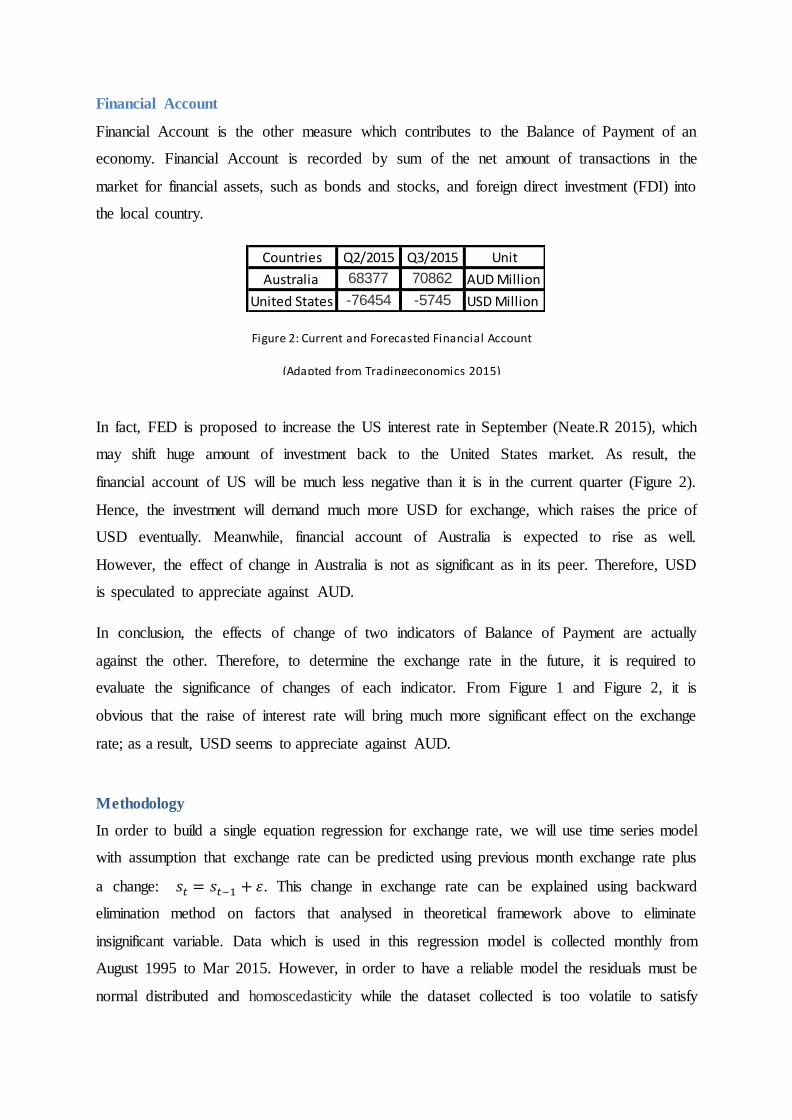
Financial Account

Financial Account is the other measure which contributes to the Balance of Payment of an

economy. Financial Account is recorded by sum of the net amount of transactions in the

market for financial assets, such as bonds and stocks, and foreign direct investment (FDI) into

the local country.

In fact, FED is proposed to increase the US interest rate in September (Neate.R 2015), which

may shift huge amount of investment back to the United States market. As result, the

financial account of US will be much less negative than it is in the current quarter (Figure 2).

Hence, the investment will demand much more USD for exchange, which raises the price of

USD eventually. Meanwhile, financial account of Australia is expected to rise as well.

However, the effect of change in Australia is not as significant as in its peer. Therefore, USD

is speculated to appreciate against AUD.

In conclusion, the effects of change of two indicators of Balance of Payment are actually

against the other. Therefore, to determine the exchange rate in the future, it is required to

evaluate the significance of changes of each indicator. From Figure 1 and Figure 2, it is

obvious that the raise of interest rate will bring much more significant effect on the exchange

rate; as a result, USD seems to appreciate against AUD.

Methodology

In order to build a single equation regression for exchange rate, we will use time series model

with assumption that exchange rate can be predicted using previous month exchange rate plus

a change: 𝑠𝑡 = 𝑠𝑡−1 + 𝜀. This change in exchange rate can be explained using backward

elimination method on factors that analysed in theoretical framework above to eliminate

insignificant variable. Data which is used in this regression model is collected monthly from

August 1995 to Mar 2015. However, in order to have a reliable model the residuals must be

normal distributed and homoscedasticity while the dataset collected is too volatile to satisfy

Countries Q2/2015 Q3/2015 Unit

Australia 68377 70862 AUD Million

United States -76454 -5745 USD Million

Figure 2: Current and Forecasted Financial Account

(Adapted from Tradingeconomics 2015)

these requirements. To solve this problem, we will transform our data by taking natural

logarithm of data or using percentage change over a periods of time depend on the pattern of

that data. The regression variables will be as follow:

𝑠𝑡 = 𝑠𝑡−1 + 𝑎1 ∗ 𝐼𝑅 + 𝑎2 ∗ 𝐶𝐼 + 𝑎3 ∗ 𝜋 + 𝑎4 ∗ 𝑚1 +𝑎5 ∗ 𝐶𝑎𝑝𝐴𝑐𝑐𝑡 + 𝑎6 ∗ 𝐸𝐺 + 𝑎7 ∗ 𝑇𝑟𝑎𝑑𝑒

Whereas:

Name of variables Description

𝑠𝑡 Natural logarithm of spot exchange rate at

period t




𝝅 Difference between monthly inflation rate of

US and AUD

M1 Natural logarithm of the ratio of US money

supply (M1) to AUD






between US and AUS

Interest rate and economic growth

Firstly, it takes time for the economy to react with information regarding economic growth

and interest rate. Therefore, in order to fit these variables into regression model we have to

estimate the lag period for them because it varies with different pairs of currency. Our

methodology is that we will run simple regression for exchange rate with four different lags

0, 1, 2 and 3 months and choose the smallest p-value for the lag periods

p-value

No lag 0.8342

1 month 0.4454

2 months 0.6226

3 months 0.2496

Refer to the figure above, we will choose 3 as our lag period for interest rate and economic

growth, the detail of regression can be found in appendix 2.

Secondly, economic growth data is for annual growth for every quarter. To fit into monthly

data we assume that both US and AUS have steady growth for 3 month in a quarter which

mean the percentage growth is the same for every month in a quarter.

Balance of payment

We split balance of payment into 3 different variables: Capital account, net trade between US

and AUS together with commodity index. We choose net trade between US and AUS rather

than Current account because only the trade between these two can affect exchange rate

directly. We include commodity index as an independent variable because most of Australia

export goods is commodity goods (Department of Foreign Affair and Trade n.d.).

As the data set is in millions of dollars, if we use data directly to run regression, the

coefficient will be zero because these numbers is way larger than natural logarithm of

exchange rate itself. Therefore we will calculate the percentage change over one month of

capital account and then compare 2 countries with each other’s. The last adjustment we made

regarding capital account is that the data is for quarterly therefore we will assume that the

growth is equal across one quarter. Let call the growth for each month in 1 quarter is x and

the growth of capital account over 3 months is r. We can have this relationship: (1 + 𝑥)3 =

1+ 𝑟 therefore the growth for a month will be 𝑥 = √(1 + 𝑟)3 − 1

Final model

After using backward elimination the first model is as below:

As we analysed before in theoretical, relative inflation rate of US/AUS will not affect spot

exchange rate. This conclusion has proven to be true by regression as the p value of inflation

rate is 0.8328 which is insignificant

After 3 more steps our final model is as below:

Iteration 1

All Variables

Regression and Correlation

Observations 233 ANOVA

R Square 0.9756 df SS MS F p value

Standard Error 0.0331 Regression 8 9.7980 1.2247 1117.6447 0.0000

Adjusted R Square 0.9747 Residual 224 0.2455 0.0011

Multiple R 0.9877 Total 232 10.0434404

Coefficients Standard Error t value p value

Intercept -0.0499 0.0283 -1.7618 0.0795

IR -0.0057 0.0025 -2.2422 0.0259

Phi -0.0004 0.0020 -0.2114 0.8328

M1 0.0113 0.0122 0.9261 0.3554

CapAcct -0.0014 0.0008 -1.8652 0.0635

Trade with US 0.0163 0.0096 1.6948 0.0915

EG -0.0038 0.0016 -2.4000 0.0172

S(t-1) 0.9549 0.0169 56.4315 0.0000

CI 0.2659 0.0765 3.4735 0.0006

Final Model






Multiple R 0.9877 Total 232 10.0434404


Intercept -0.0252 0.0070 -3.5705 0.0004

IR -0.0057 0.0022 -2.5507 0.0114

CapAcct -0.0015 0.0008 -1.9204 0.0561

Trade with US 0.0160 0.0096 1.6683 0.0966

EG -0.0033 0.0015 -2.2757 0.0238

S(t-1) 0.9546 0.0149 64.0084 0.0000

CI 0.2440 0.0724 3.3685 0.0009

Forecast?

R Square = 97.55% means that 97.55% the variation of exchange rate can be explain by the

variation of independent variables used in our model.

Variables Coefficient Explanation

𝑠𝑡−1

0.9546 If the natural log of lag

exchange rate increase by 1 the

spot exchange rate will

increase by 0.9546

IR

-0.0057 If the different of interest rate

between US to AUS widen, the

exchange rate will decrease

which will lead to the

depreciation of AUD

CI 0.244 If the commodity price in AUS

increase AUD will appreciate

CapAcct

-0.0015 If the change in capital account

of US is relatively larger than

AUS then the AUD will

depreciate

EG

-0.0033 If the economic growth of US

relatively higher than AUS

then the AUD will depreciate

Trade

0.016 If net trade from AUS to US

increase then the AUD will

appreciate against the US

Residuals

-0.2000

-0.1000

0.0000

0.1000

0 100 200 300

Re

sid

ual

s

Observations

Series1

The residuals are spreading along the 0 line and has no clear pattern which indicate that this

model is significant

Histogram of residuals is normally distributed

Conclusion & Limitation

Conclusion

Using the analysis above we can conclude that this model can be used to predict spot

exchange rate with significance level of 90%. The final equation is:

𝑠𝑡 = −0.0252 + 0.9546 ∗ 𝑠𝑡−1 −0.0057 ∗ 𝐼𝑅 + 0.244 ∗ 𝐶𝐼 − 0.0015 ∗ 𝐶𝑎𝑝𝐴𝑐𝑐𝑡 − 0.0033

∗ 𝐸𝐺 + 0.016 ∗ 𝑇𝑟𝑎𝑑𝑒

Whereas:

Variables Description

𝑠𝑡−1 Natural logarithm of spot exchange rate at

previous month









between US and AUS

0

20

40

60

Fre

qu

en

cy

Variable

Residuals

Series1

Forecasted data at 28/8:

Variables Forecasted value Assumption

𝑠𝑡−1 Ln(0.73067)= - 0.31379

IR Ln(0.25/2)= - 2.07944

CI

Ln(61*(1-1.6%)/61) = -0.01613

(Reserve Bank of Australia(RBA) 2015)

The commodity index of Australia

has been decreasing for the last four

years with the average of 1.6%

(appendix ) so we assume that it will

decrease by this rate between July

and August 2015

CapAcct 0.231969766

The calculation is in appendix 3

EG 0.45

Trade

0.74% According to trading economics the

current account of Australia will

improve by 2.26% from Q2/2015 to

Q3/2015. We assume that net trade

between US and AUS will has the

same increase therefore monthly

growth will be

0.74%=√(1 + 2.26%)3 −1

Using figured above we can calculate the forecasted spot exchange rate at 28/8/2015:

ln(𝑠𝑎𝑢𝑔−15) = −0.0252 − 0.31379 ∗ 0.9546 − 0.0057 ∗ (−2.07944)+ 0.244

∗ (−0.01613) − 0.0015 ∗ (0.23197) − 0.0033 ∗ 0.45 + 0.016 ∗ 0.0074

= −0.31854

Therefore the spot exchange rate will be 𝑠𝑎𝑢𝑔−15 = 0.727209

Limitations

Even though this model looks fantastic with very high R squared and acceptable residuals

plot, its prediction power is not too credible. If we calculate the percentage change from a

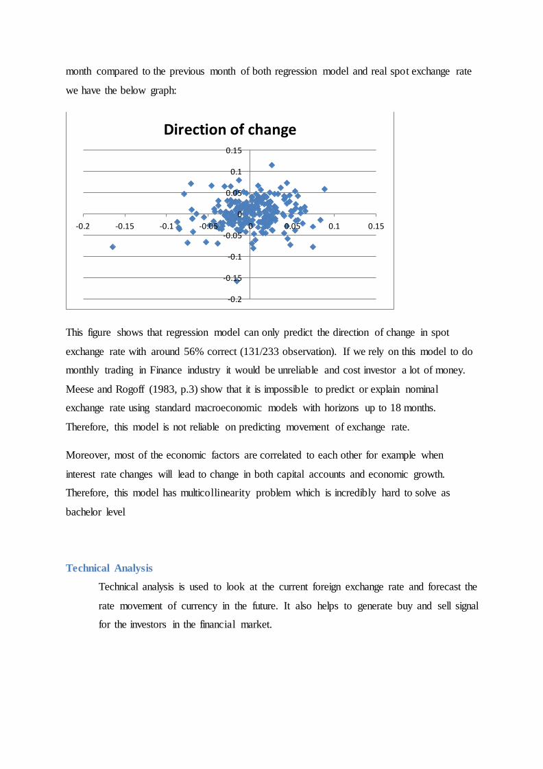
month compared to the previous month of both regression model and real spot exchange rate

we have the below graph:

This figure shows that regression model can only predict the direction of change in spot

exchange rate with around 56% correct (131/233 observation). If we rely on this model to do

monthly trading in Finance industry it would be unreliable and cost investor a lot of money.

Meese and Rogoff (1983, p.3) show that it is impossible to predict or explain nominal

exchange rate using standard macroeconomic models with horizons up to 18 months.

Therefore, this model is not reliable on predicting movement of exchange rate.

Moreover, most of the economic factors are correlated to each other for example when

interest rate changes will lead to change in both capital accounts and economic growth.

Therefore, this model has multicollinearity problem which is incredibly hard to solve as

bachelor level

Technical Analysis

Technical analysis is used to look at the current foreign exchange rate and forecast the

rate movement of currency in the future. It also helps to generate buy and sell signal

for the investors in the financial market.

-0.2

-0.15

-0.1

-0.05

0

0.05

0.1

0.15

-0.2 -0.15 -0.1 -0.05 0 0.05 0.1 0.15

Direction of change

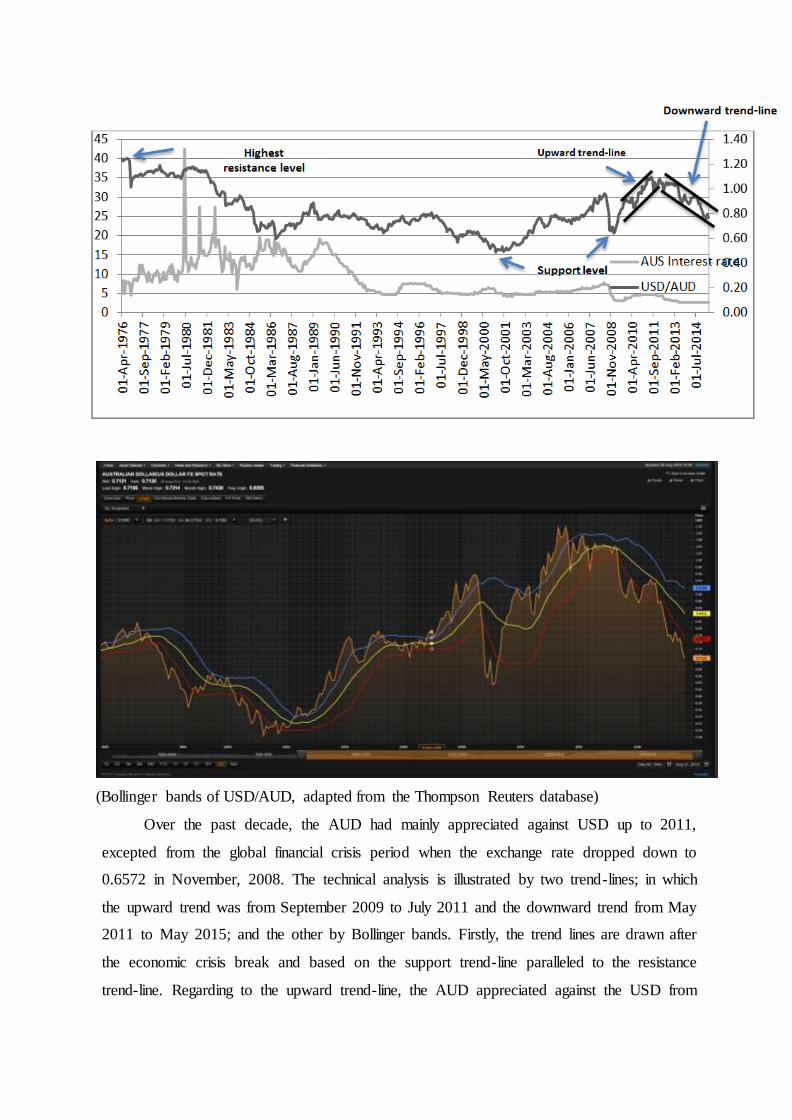
(Bollinger bands of USD/AUD, adapted from the Thompson Reuters database)

Over the past decade, the AUD had mainly appreciated against USD up to 2011,

excepted from the global financial crisis period when the exchange rate dropped down to

0.6572 in November, 2008. The technical analysis is illustrated by two trend-lines; in which

the upward trend was from September 2009 to July 2011 and the downward trend from May

2011 to May 2015; and the other by Bollinger bands. Firstly, the trend lines are drawn after

the economic crisis break and based on the support trend-line paralleled to the resistance

trend-line. Regarding to the upward trend-line, the AUD appreciated against the USD from

the increase of 0.8801 to 1.0954 (around 21%) due to the result of trade and strong economic

performance after the crisis, especially the rises in interest rate. However, the resistance

level in July, 2011 was followed by the downward trend-line to May, 2015 at 0.7663 which

means that the USD appreciated against the AUD. The reason for this depreciation because

of the weak commodity prices, the decline of the mining – investment boom, the lower-than-

expected growth in their big trading partner- China and the US economy recovery.

Secondly, the Bollinger band shows two standard deviations away from the 20 months

average moving. It also shows the trends and measures the volatility of the currency’s price;

the wider the bands, the more volatility between two currencies, vice versa. Comparing the

two periods before and after financial crisis in 2008, the bands became from contracted –

less volatility to widen – more volatility due to the fluctuations in economic factors as

mentioned above. As a result of the more volatility, the USD/AUD will not be stable in the

future which increases risk in investment. The investors are prefer to buy at lower rate and

sell at the higher rate, the technical analysis shows that there will be the disadvantages for

AUD since the trend line has declined and volatility of USD/AUD has increased in recent

years.

Reference

Banet J, Hayes B 2015, “U.S inflation outlook 2015: The Fed versus market”,

February 2015, viewed August 28 2015, available from:

<http://www.federalreserve.gov/faqs/economy_14400.htm>

Board of Governors of Federal Reserve System n.d , Selected Interest rates, viewed

20 August 20015 ; <http://www.federalreserve.gov/releases/h15/data.htm>

Bloomberg 2015, “Americans gaining Confidence as Job Market Strengthens:

Economy”, January 2015, viewed 27 August 2015,

<http://www.bloomberg.com/news/articles/2015-01-08/u-s-consumer-confidence-

rebounded-to-seven-year-high- last-week>

Department of Foreign Affair and Trade, ‘Australia’s Top 10 goods & services

exports and imports, < http://dfat.gov.au/trade/resources/trade-at-a-glance/pages/top-

goods-services.aspx>

Federal Reserve 2015, “why are interest rates being kept at a low level?” , viewed

August 27 2015, <http://money.cnn.com/2015/03/16/investing/us-dollar-fastest-rise-

40-years/>

International Monetary Fund n.d, ‘e-Library data – International Financial Statistics’,

viewed August 17 2015; <http://elibrary-data.imf.org/DataExplorer.aspx>

Neate. R 2015, The Guardian, “Federal Reserve moves toward raising interest rate

for first time in year”, viewed on August 22, 2015,

<http://www.theguardian.com/business/2015/aug/19/federal-reserve-interest-rate-

increase>

Oanda (n.d), “Exchange rate dynamics and currency factors”, viewed August 27

2015, <http://fxtrade.oanda.ca/learn/top-5-factors-that-affect-exchange-rates>

Meese & Rogoff 1983, ‘Empirical Exchange rate models of the seventies’, Journal of

International Economics, vol 14, p3-24

Reserve Bank of Australia(RBA) 2015, Index of Commodity Prices, viewed August

27 2015, <http://www.rba.gov.au/statistics/frequency/commodity-prices.html>

Rogoff. K 1996, ‘The Purchasing Power Parity Puzzles’, Journal of Economic

Literature, June 1996, Vol. XXXIV, pp. 647-668

http://www.federalreserve.gov/faqs/economy_14400.htm

http://www.bloomberg.com/news/articles/2015-01-08/u-s-consumer-confidence-rebounded-to-seven-year-high-last-week

http://www.bloomberg.com/news/articles/2015-01-08/u-s-consumer-confidence-rebounded-to-seven-year-high-last-week

http://dfat.gov.au/trade/resources/trade-at-a-glance/pages/top-goods-services.aspx

http://dfat.gov.au/trade/resources/trade-at-a-glance/pages/top-goods-services.aspx

http://money.cnn.com/2015/03/16/investing/us-dollar-fastest-rise-40-years/

http://money.cnn.com/2015/03/16/investing/us-dollar-fastest-rise-40-years/

http://www.theguardian.com/business/2015/aug/19/federal-reserve-interest-rate-increase

http://www.theguardian.com/business/2015/aug/19/federal-reserve-interest-rate-increase

http://fxtrade.oanda.ca/learn/top-5-factors-that-affect-exchange-rates

Tradingeconomics n.d, Trading Economics, “Australia Capital Flows Forecast”

viewed on August 22, 2015, <http://www.tradingeconomics.com/australia/capital-

flows/forecast>

Tradingeconomics n.d, Trading Economics, “Australia Foreign Direct Investment

Forecast” viewed on August 22, 2015,

<http://www.tradingeconomics.com/australia/foreign-direct- investment/forecast>

Tradingeconomics n.d, Trading Economics, “United States Capital Flows Forecast”

viewed on August 22, 2015, <http://www.tradingeconomics.com/united-states/capital-

flows/forecast>

Tradingeconomics n.d, Trading Economics, “United States Foreign Direct Investment

Forecast” viewed on August 22, 2015, <http://www.tradingeconomics.com/united-

states/foreign-direct- investment/forecast>

http://www.tradingeconomics.com/australia/capital-flows/forecast

http://www.tradingeconomics.com/australia/capital-flows/forecast

http://www.tradingeconomics.com/australia/foreign-direct-investment/forecast

http://www.tradingeconomics.com/united-states/capital-flows/forecast

http://www.tradingeconomics.com/united-states/capital-flows/forecast

http://www.tradingeconomics.com/united-states/foreign-direct-investment/forecast

http://www.tradingeconomics.com/united-states/foreign-direct-investment/forecast

Appendix

S(t) IR Phi M1 CapAcct Trade with USEG

31-Aug-1995 -0.28449 -0.22547 -2.522550336 2.699055 -2.57325 0.224193 -0.33349

30-Sep-1995 -0.28104 -0.23639 -2.596492637 2.693099 -2.57325 -0.12538 -0.33349

31-Oct-1995 -0.27892 -0.26039 -2.290635452 2.683907 0.379024 0.112287 -0.96577

30-Nov-1995 -0.29182 -0.26744 -2.494789579 2.678 0.379024 0.118353 -0.96577

31-Dec-1995 -0.29437 -0.25705 -2.561589846 2.648659 0.379024 -0.21432 -0.96577

31-Jan-1996 -0.29477 -0.27061 -1.032122422 2.631853 -1.17814 0.244776 -1.48827

29-Feb-1996 -0.26984 -0.26369 -1.109237906 2.617558 -1.17814 0.00953 -1.48827

31-Mar-1996 -0.24936 -0.29214 -0.91984148 2.60487 -1.17814 -0.02872 -1.48827

30-Apr-1996 -0.24156 -0.2993 -0.193357472 2.590832 0.084846 0.055542 -2.42684

31-May-1996 -0.22527 -0.3664 -0.199067017 2.582333 0.084846 0.0504 -2.42684

30-Jun-1996 -0.23699 -0.34664 -0.335901639 2.570112 0.084846 -0.20288 -2.42684

31-Jul-1996 -0.25735 -0.3664 0.810819672 2.564109 -0.22669 0.208025 -0.23625

31-Aug-1996 -0.23458 -0.36257 0.737697842 2.551946 -0.22669 -0.07628 -0.23625

30-Sep-1996 -0.23269 -0.3648 0.862610966 2.533109 -0.22669 -0.12954 -0.23625

31-Oct-1996 -0.23332 -0.27229 1.472843201 2.52295 0.071549 0.201169 0.335276

30-Nov-1996 -0.20986 -0.27612 1.735208333 2.494316 0.071549 -0.16669 0.335276

31-Dec-1996 -0.22753 -0.28106 1.80247557 2.463444 0.071549 0.166506 0.335276

31-Jan-1997 -0.27181 -0.29671 1.684041451 2.45948 -2.74065 -0.10415 0.359008

28-Feb-1997 -0.25386 -0.19294 1.674215623 2.464805 -2.74065 -0.18442 0.359008

31-Mar-1997 -0.24016 -0.13919 1.401721259 2.43913 -2.74065 0.168591 0.359008

30-Apr-1997 -0.24705 -0.13852 2.195201536 2.427326 -2.39195 0.02483 1.870348

31-May-1997 -0.27273 -0.14669 1.934993614 2.405161 -2.39195 0.003888 1.870348

30-Jun-1997 -0.2937 -0.1221 1.997383535 2.395214 -2.39195 0.187602 1.870348

31-Jul-1997 -0.2941 -0.09679 2.679299363 2.386185 -0.4339 -0.14609 -1.0187

31-Aug-1997 -0.3087 0.007299 2.67504768 2.368531 -0.4339 -0.09208 -1.0187

30-Sep-1997 -0.32878 -0.01606 2.604626109 2.358701 -0.4339 0.069637 -1.0187

31-Oct-1997 -0.35155 0.100942 2.3846494 2.345841 0.207516 0.047049 0.691546

30-Nov-1997 -0.38522 0.13508 2.128499369 2.322558 0.207516 -0.23231 0.691546

31-Dec-1997 -0.42664 0.102557 2.002395965 2.323759 0.207516 0.243714 0.691546

31-Jan-1998 -0.40152 0.093312 1.721338781 2.324581 0.187518 -0.06548 -0.52394

28-Feb-1998 -0.39378 0.08899 1.591102757 2.31882 0.187518 -0.11374 -0.52394

31-Mar-1998 -0.41038 0.058014 1.525 2.323074 0.187518 0.134036 -0.52394

30-Apr-1998 -0.43094 0.102168 0.685705368 2.330649 0.614298 -0.03819 -1.18925

31-May-1998 -0.47225 0.095129 0.936445971 2.31261 0.614298 -0.07517 -1.18925

30-Jun-1998 -0.48858 0.09349 0.934341859 2.297284 0.614298 0.051036 -1.18925

31-Jul-1998 -0.49217 0.086178 0.332242991 2.289383 -2.63374 0.217037 0.41652

31-Aug-1998 -0.5637 0.107589 0.266915423 2.27443 -2.63374 -0.24202 0.41652

30-Sep-1998 -0.52003 0.10616 0.138833747 2.275509 -2.63374 0.040248 0.41652

31-Oct-1998 -0.46793 0.108575 -0.014851485 2.279791 0.404867 0.426599 -1.50834

30-Nov-1998 -0.45839 0.102362 0.047987616 2.280373 0.404867 -0.12459 -1.50834

31-Dec-1998 -0.48792 0.095129 0.111903286 2.280106 0.404867 -0.17907 -1.50834

31-Jan-1999 -0.46426 0.060995 0.480792079 2.284471 -2.24123 -0.03464 -0.44593

28-Feb-1999 -0.47401 -0.03259 0.415929586 2.267831 -2.24123 -0.12676 -0.44593

31-Mar-1999 -0.46315 -0.00639 0.536263872 2.258782 -2.24123 0.244227 -0.44593

30-Apr-1999 -0.41582 -0.02137 1.236923077 2.254893 0.191636 -0.0656 -0.04695

31-May-1999 -0.43217 -0.0146 1.048452088 2.251955 0.191636 0.025673 -0.04695

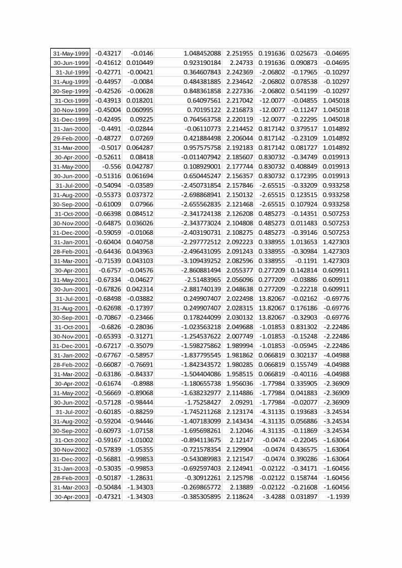
31-May-1999 -0.43217 -0.0146 1.048452088 2.251955 0.191636 0.025673 -0.04695

30-Jun-1999 -0.41612 0.010449 0.923190184 2.24733 0.191636 0.090873 -0.04695

31-Jul-1999 -0.42771 -0.00421 0.364607843 2.242369 -2.06802 -0.17965 -0.10297

31-Aug-1999 -0.44957 -0.0084 0.484381885 2.234642 -2.06802 0.078538 -0.10297

30-Sep-1999 -0.42526 -0.00628 0.848361858 2.227336 -2.06802 0.541199 -0.10297

31-Oct-1999 -0.43913 0.018201 0.64097561 2.217042 -12.0077 -0.04855 1.045018

30-Nov-1999 -0.45004 0.060995 0.70195122 2.216873 -12.0077 -0.11247 1.045018

31-Dec-1999 -0.42495 0.09225 0.764563758 2.220119 -12.0077 -0.22295 1.045018

31-Jan-2000 -0.4491 -0.02844 -0.06110773 2.214452 0.817142 0.379517 1.014892

29-Feb-2000 -0.48727 0.07269 0.421884498 2.206044 0.817142 -0.23109 1.014892

31-Mar-2000 -0.5017 0.064287 0.957575758 2.192183 0.817142 0.081727 1.014892

30-Apr-2000 -0.52611 0.08418 -0.011407942 2.185607 0.830732 -0.34749 0.019913

31-May-2000 -0.556 0.042787 0.108929001 2.177744 0.830732 0.408849 0.019913

30-Jun-2000 -0.51316 0.061694 0.650445247 2.156357 0.830732 0.172395 0.019913

31-Jul-2000 -0.54094 -0.03589 -2.450731854 2.157846 -2.65515 -0.33209 0.933258

31-Aug-2000 -0.55373 0.037372 -2.698868941 2.150132 -2.65515 0.123515 0.933258

30-Sep-2000 -0.61009 0.07966 -2.655562835 2.121468 -2.65515 0.107924 0.933258

31-Oct-2000 -0.66398 0.084512 -2.341724138 2.126208 0.485273 -0.14351 0.507253

30-Nov-2000 -0.64875 0.036026 -2.343773024 2.104808 0.485273 0.011483 0.507253

31-Dec-2000 -0.59059 -0.01068 -2.403190731 2.108275 0.485273 -0.39146 0.507253

31-Jan-2001 -0.60404 0.040758 -2.297772512 2.092223 0.338955 1.013653 1.427303

28-Feb-2001 -0.64436 0.043963 -2.496431095 2.091243 0.338955 -0.30984 1.427303

31-Mar-2001 -0.71539 0.043103 -3.109439252 2.082596 0.338955 -0.1191 1.427303

30-Apr-2001 -0.6757 -0.04576 -2.860881494 2.055377 0.277209 0.142814 0.609911

31-May-2001 -0.67334 -0.04627 -2.51483965 2.056096 0.277209 -0.03886 0.609911

30-Jun-2001 -0.67826 0.042314 -2.881740139 2.048638 0.277209 -0.22218 0.609911

31-Jul-2001 -0.68498 -0.03882 0.249907407 2.022498 13.82067 -0.02162 -0.69776

31-Aug-2001 -0.62698 -0.17397 0.249907407 2.028315 13.82067 0.176186 -0.69776

30-Sep-2001 -0.70867 -0.23466 0.178244099 2.030132 13.82067 -0.32903 -0.69776

31-Oct-2001 -0.6826 -0.28036 -1.023563218 2.049688 -1.01853 0.831302 -2.22486

30-Nov-2001 -0.65393 -0.31271 -1.254537622 2.007749 -1.01853 -0.15248 -2.22486

31-Dec-2001 -0.67217 -0.35079 -1.598275862 1.989994 -1.01853 -0.05945 -2.22486

31-Jan-2002 -0.67767 -0.58957 -1.837795545 1.981862 0.066819 0.302137 -4.04988

28-Feb-2002 -0.66087 -0.76691 -1.842343572 1.980285 0.066819 0.155749 -4.04988

31-Mar-2002 -0.63186 -0.84337 -1.504404086 1.958515 0.066819 -0.40116 -4.04988

30-Apr-2002 -0.61674 -0.8988 -1.180655738 1.956036 -1.77984 0.335905 -2.36909

31-May-2002 -0.56669 -0.89068 -1.638232977 2.114886 -1.77984 0.041883 -2.36909

30-Jun-2002 -0.57128 -0.98444 -1.75258427 2.09291 -1.77984 -0.02077 -2.36909

31-Jul-2002 -0.60185 -0.88259 -1.745211268 2.123174 -4.31135 0.193683 -3.24534

31-Aug-2002 -0.59204 -0.94446 -1.407183099 2.143434 -4.31135 0.056886 -3.24534

30-Sep-2002 -0.60973 -1.07158 -1.695698261 2.12046 -4.31135 -0.11869 -3.24534

31-Oct-2002 -0.59167 -1.01002 -0.894113675 2.12147 -0.0474 -0.22045 -1.63064

30-Nov-2002 -0.57839 -1.05355 -0.721578354 2.129904 -0.0474 0.436575 -1.63064

31-Dec-2002 -0.56881 -0.99853 -0.543089983 2.121547 -0.0474 0.390286 -1.63064

31-Jan-2003 -0.53035 -0.99853 -0.692597403 2.124941 -0.02122 -0.34171 -1.60456

28-Feb-2003 -0.50187 -1.28631 -0.30912261 2.125798 -0.02122 0.158744 -1.60456

31-Mar-2003 -0.50484 -1.34303 -0.269865772 2.13889 -0.02122 -0.21608 -1.60456

30-Apr-2003 -0.47321 -1.34303 -0.385305895 2.118624 -3.4288 0.031897 -1.1939

31-Mar-2003 -0.50484 -1.34303 -0.269865772 2.13889 -0.02122 -0.21608 -1.60456

30-Apr-2003 -0.47321 -1.34303 -0.385305895 2.118624 -3.4288 0.031897 -1.1939

31-May-2003 -0.4274 -1.32493 -0.552157953 2.116751 -3.4288 0.063212 -1.1939

30-Jun-2003 -0.40437 -1.335 -0.497715397 2.116426 -3.4288 0.570351 -1.1939

31-Jul-2003 -0.42633 -1.32703 -0.480061077 2.117496 0.133039 -0.39156 0.005746

31-Aug-2003 -0.44629 -1.33333 -0.431726619 2.131094 0.133039 0.298569 0.005746

30-Sep-2003 -0.38552 -1.35929 -0.269558011 2.129143 0.133039 0.101258 0.005746

31-Oct-2003 -0.35013 -1.54819 -0.409183673 2.125976 0.279358 -0.09061 0.02115

30-Nov-2003 -0.32767 -1.54942 -0.684969664 2.122322 0.279358 -0.28466 0.02115

31-Dec-2003 -0.28768 -1.54819 -0.570508568 2.113843 0.279358 0.177126 0.02115

31-Jan-2004 -0.26866 -1.54819 -0.113747936 2.116851 -3.23939 0.122473 0.309425

29-Feb-2004 -0.26033 -1.68825 -0.3469361 2.099716 -3.23939 -0.12408 0.309425

31-Mar-2004 -0.27589 -1.67843 -0.302757872 2.106146 -3.23939 0.405283 0.309425

30-Apr-2004 -0.32573 -1.72811 -0.254907508 2.117672 0.652806 -0.18407 -0.38132

31-May-2004 -0.33645 -1.7146 0.511771117 2.118393 0.652806 0.012268 -0.38132

30-Jun-2004 -0.37266 -1.65823 0.726194883 2.122563 0.652806 -0.06912 -0.38132

31-Jul-2004 -0.35868 -1.65823 0.710755846 2.126631 0.518678 0.191095 -0.36534

31-Aug-2004 -0.3551 -1.65823 0.374387866 2.123681 0.518678 -0.00601 -0.36534

30-Sep-2004 -0.33589 -1.62867 0.257796976 2.124837 0.518678 0.122935 -0.36534

31-Oct-2004 -0.2929 -1.46999 0.669189189 2.122774 -1.28243 -0.31637 -0.45284

30-Nov-2004 -0.25167 -1.30055 1.00303523 2.108282 -1.28243 0.274611 -0.45284

31-Dec-2004 -0.24974 -1.18199 0.735561584 2.118507 -1.28243 0.106428 -0.45284

31-Jan-2005 -0.25567 -1.12663 0.599762419 2.120887 -4.05742 -0.0084 0.182399

28-Feb-2005 -0.23509 -1.00071 0.637518797 2.095738 -4.05742 -0.12911 0.182399

31-Mar-2005 -0.2589 -0.88812 0.778345784 2.10347 -4.05742 0.356564 0.182399

30-Apr-2005 -0.24705 -0.83405 1.030638298 2.094511 0.313079 -0.08488 0.563855

31-May-2005 -0.28011 -0.74194 0.322749868 2.077144 0.313079 -0.10548 0.563855

30-Jun-2005 -0.26958 -0.73784 0.050311017 2.07004 0.313079 -0.09573 0.563855

31-Jul-2005 -0.27509 -0.71442 0.077898627 2.079642 4.634925 0.303533 0.395284

31-Aug-2005 -0.29156 -0.60689 0.55116095 2.058338 4.634925 -0.04237 0.395284

30-Sep-2005 -0.27247 -0.59289 1.596677199 2.066674 4.634925 -0.13254 0.395284

31-Oct-2005 -0.28942 -0.54816 1.527826087 2.062497 -1.03663 -0.08173 -0.04449

30-Nov-2005 -0.30259 -0.45199 0.635497382 2.056695 -1.03663 0.262936 -0.04449

31-Dec-2005 -0.30966 -0.41827 0.595659485 2.054944 -1.03663 -0.19491 -0.04449

31-Jan-2006 -0.28635 -0.37502 1.065317252 2.040573 -8.37724 0.601303 -0.37326

28-Feb-2006 -0.30354 -0.31845 0.677497393 2.036871 -8.37724 -0.40043 -0.37326

31-Mar-2006 -0.33421 -0.30437 0.442648733 2.031596 -8.37724 0.353714 -0.37326

30-Apr-2006 -0.2821 -0.24846 -0.454265159 2.004043 0.168803 -0.18225 0.437012

31-May-2006 -0.26971 -0.2029 0.166666667 2.000464 0.168803 0.335092 0.437012

30-Jun-2006 -0.29666 -0.18087 0.318766067 1.998319 0.168803 -0.05934 0.437012

31-Jul-2006 -0.26683 -0.19305 0.185342886 1.978468 0.211136 -0.05187 0.482586

31-Aug-2006 -0.27089 -0.15183 -0.141262729 1.96866 0.211136 0.202043 0.482586

30-Sep-2006 -0.29035 -0.14176 -1.897625755 1.965727 0.211136 -0.16205 0.482586

31-Oct-2006 -0.2624 -0.09288 -2.034779116 1.950798 -4.3698 0.138242 -0.11107

30-Nov-2006 -0.24207 -0.13353 -1.366315789 1.944175 -4.3698 -0.0777 -0.11107

31-Dec-2006 -0.23408 -0.16632 -0.799349593 1.928371 -4.3698 0.080618 -0.11107

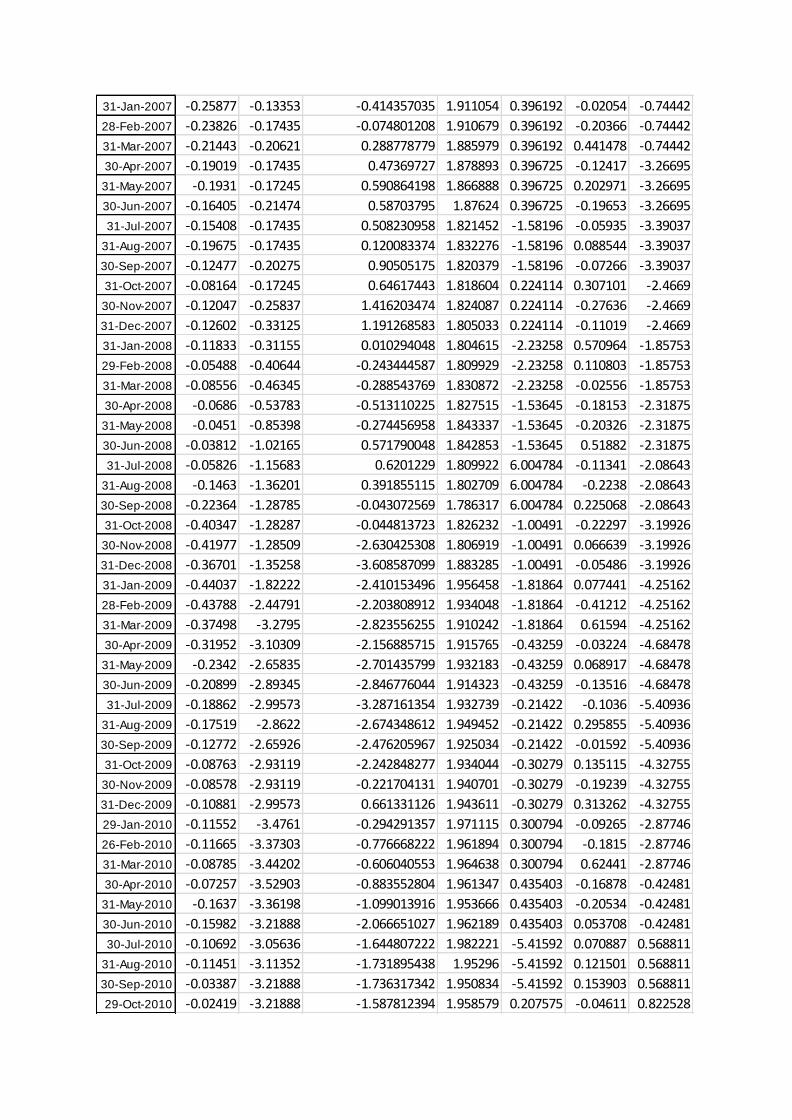
31-Jan-2007 -0.25877 -0.13353 -0.414357035 1.911054 0.396192 -0.02054 -0.74442

28-Feb-2007 -0.23826 -0.17435 -0.074801208 1.910679 0.396192 -0.20366 -0.74442

31-Mar-2007 -0.21443 -0.20621 0.288778779 1.885979 0.396192 0.441478 -0.74442

30-Apr-2007 -0.19019 -0.17435 0.47369727 1.878893 0.396725 -0.12417 -3.26695

31-May-2007 -0.1931 -0.17245 0.590864198 1.866888 0.396725 0.202971 -3.26695

30-Jun-2007 -0.16405 -0.21474 0.58703795 1.87624 0.396725 -0.19653 -3.26695

31-Jul-2007 -0.15408 -0.17435 0.508230958 1.821452 -1.58196 -0.05935 -3.39037

31-Aug-2007 -0.19675 -0.17435 0.120083374 1.832276 -1.58196 0.088544 -3.39037

30-Sep-2007 -0.12477 -0.20275 0.90505175 1.820379 -1.58196 -0.07266 -3.39037

31-Oct-2007 -0.08164 -0.17245 0.64617443 1.818604 0.224114 0.307101 -2.4669

30-Nov-2007 -0.12047 -0.25837 1.416203474 1.824087 0.224114 -0.27636 -2.4669

31-Dec-2007 -0.12602 -0.33125 1.191268583 1.805033 0.224114 -0.11019 -2.4669

31-Jan-2008 -0.11833 -0.31155 0.010294048 1.804615 -2.23258 0.570964 -1.85753

29-Feb-2008 -0.05488 -0.40644 -0.243444587 1.809929 -2.23258 0.110803 -1.85753

31-Mar-2008 -0.08556 -0.46345 -0.288543769 1.830872 -2.23258 -0.02556 -1.85753

30-Apr-2008 -0.0686 -0.53783 -0.513110225 1.827515 -1.53645 -0.18153 -2.31875

31-May-2008 -0.0451 -0.85398 -0.274456958 1.843337 -1.53645 -0.20326 -2.31875

30-Jun-2008 -0.03812 -1.02165 0.571790048 1.842853 -1.53645 0.51882 -2.31875

31-Jul-2008 -0.05826 -1.15683 0.6201229 1.809922 6.004784 -0.11341 -2.08643

31-Aug-2008 -0.1463 -1.36201 0.391855115 1.802709 6.004784 -0.2238 -2.08643

30-Sep-2008 -0.22364 -1.28785 -0.043072569 1.786317 6.004784 0.225068 -2.08643

31-Oct-2008 -0.40347 -1.28287 -0.044813723 1.826232 -1.00491 -0.22297 -3.19926

30-Nov-2008 -0.41977 -1.28509 -2.630425308 1.806919 -1.00491 0.066639 -3.19926

31-Dec-2008 -0.36701 -1.35258 -3.608587099 1.883285 -1.00491 -0.05486 -3.19926

31-Jan-2009 -0.44037 -1.82222 -2.410153496 1.956458 -1.81864 0.077441 -4.25162

28-Feb-2009 -0.43788 -2.44791 -2.203808912 1.934048 -1.81864 -0.41212 -4.25162

31-Mar-2009 -0.37498 -3.2795 -2.823556255 1.910242 -1.81864 0.61594 -4.25162

30-Apr-2009 -0.31952 -3.10309 -2.156885715 1.915765 -0.43259 -0.03224 -4.68478

31-May-2009 -0.2342 -2.65835 -2.701435799 1.932183 -0.43259 0.068917 -4.68478

30-Jun-2009 -0.20899 -2.89345 -2.846776044 1.914323 -0.43259 -0.13516 -4.68478

31-Jul-2009 -0.18862 -2.99573 -3.287161354 1.932739 -0.21422 -0.1036 -5.40936

31-Aug-2009 -0.17519 -2.8622 -2.674348612 1.949452 -0.21422 0.295855 -5.40936

30-Sep-2009 -0.12772 -2.65926 -2.476205967 1.925034 -0.21422 -0.01592 -5.40936

31-Oct-2009 -0.08763 -2.93119 -2.242848277 1.934044 -0.30279 0.135115 -4.32755

30-Nov-2009 -0.08578 -2.93119 -0.221704131 1.940701 -0.30279 -0.19239 -4.32755

31-Dec-2009 -0.10881 -2.99573 0.661331126 1.943611 -0.30279 0.313262 -4.32755

29-Jan-2010 -0.11552 -3.4761 -0.294291357 1.971115 0.300794 -0.09265 -2.87746

26-Feb-2010 -0.11665 -3.37303 -0.776668222 1.961894 0.300794 -0.1815 -2.87746

31-Mar-2010 -0.08785 -3.44202 -0.606040553 1.964638 0.300794 0.62441 -2.87746

30-Apr-2010 -0.07257 -3.52903 -0.883552804 1.961347 0.435403 -0.16878 -0.42481

31-May-2010 -0.1637 -3.36198 -1.099013916 1.953666 0.435403 -0.20534 -0.42481

30-Jun-2010 -0.15982 -3.21888 -2.066651027 1.962189 0.435403 0.053708 -0.42481

30-Jul-2010 -0.10692 -3.05636 -1.644807222 1.982221 -5.41592 0.070887 0.568811

31-Aug-2010 -0.11451 -3.11352 -1.731895438 1.95296 -5.41592 0.121501 0.568811

30-Sep-2010 -0.03387 -3.21888 -1.736317342 1.950834 -5.41592 0.153903 0.568811

29-Oct-2010 -0.02419 -3.21888 -1.587812394 1.958579 0.207575 -0.04611 0.822528

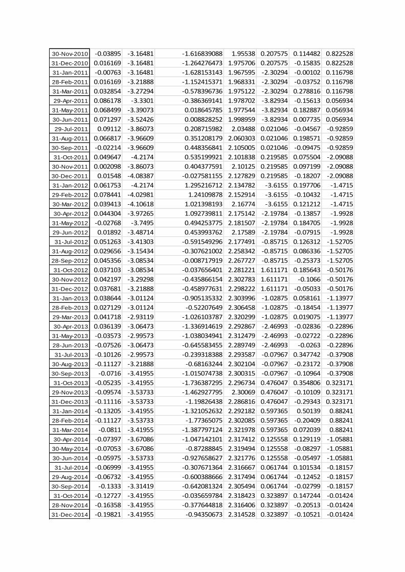
30-Nov-2010 -0.03895 -3.16481 -1.616839088 1.95538 0.207575 0.114482 0.822528

31-Dec-2010 0.016169 -3.16481 -1.264276473 1.975706 0.207575 -0.15835 0.822528

31-Jan-2011 -0.00763 -3.16481 -1.628153143 1.967595 -2.30294 -0.00102 0.116798

28-Feb-2011 0.016169 -3.21888 -1.152415371 1.968331 -2.30294 -0.03752 0.116798

31-Mar-2011 0.032854 -3.27294 -0.578396736 1.975122 -2.30294 0.278816 0.116798

29-Apr-2011 0.086178 -3.3301 -0.386369141 1.978702 -3.82934 -0.15613 0.056934

31-May-2011 0.068499 -3.39073 0.018645785 1.977544 -3.82934 0.182887 0.056934

30-Jun-2011 0.071297 -3.52426 0.008828252 1.998959 -3.82934 0.007735 0.056934

29-Jul-2011 0.09112 -3.86073 0.208715982 2.03488 0.021046 -0.04567 -0.92859

31-Aug-2011 0.066817 -3.96609 0.351208179 2.060303 0.021046 0.198571 -0.92859

30-Sep-2011 -0.02214 -3.96609 0.448356841 2.105005 0.021046 -0.09475 -0.92859

31-Oct-2011 0.049647 -4.2174 0.535199921 2.101838 0.219585 0.075504 -2.09088

30-Nov-2011 0.002098 -3.86073 0.404377591 2.10125 0.219585 0.097199 -2.09088

30-Dec-2011 0.01548 -4.08387 -0.027581155 2.127829 0.219585 -0.18207 -2.09088

31-Jan-2012 0.061753 -4.2174 1.295216712 2.134782 -3.6155 0.197706 -1.4715

29-Feb-2012 0.078441 -4.02981 1.24109878 2.152914 -3.6155 -0.10432 -1.4715

30-Mar-2012 0.039413 -4.10618 1.021398193 2.16774 -3.6155 0.121212 -1.4715

30-Apr-2012 0.044304 -3.97265 1.092739811 2.175142 -2.19784 -0.13857 -1.9928

31-May-2012 -0.02768 -3.7495 0.494253775 2.181507 -2.19784 0.184705 -1.9928

29-Jun-2012 0.01892 -3.48714 0.453993762 2.17589 -2.19784 -0.07915 -1.9928

31-Jul-2012 0.051263 -3.41303 -0.591549296 2.177491 -0.85715 0.126312 -1.52705

31-Aug-2012 0.029656 -3.15434 -0.307621002 2.258342 -0.85715 0.086336 -1.52705

28-Sep-2012 0.045356 -3.08534 -0.008717919 2.267727 -0.85715 -0.25373 -1.52705

31-Oct-2012 0.037103 -3.08534 -0.037656401 2.281221 1.611171 0.185643 -0.50176

30-Nov-2012 0.042197 -3.29298 -0.435866154 2.302783 1.611171 -0.1066 -0.50176

31-Dec-2012 0.037681 -3.21888 -0.458977631 2.298222 1.611171 -0.05033 -0.50176

31-Jan-2013 0.038644 -3.01124 -0.905135332 2.303996 -1.02875 0.058161 -1.13977

28-Feb-2013 0.027129 -3.01124 -0.52207649 2.306458 -1.02875 -0.18454 -1.13977

29-Mar-2013 0.041718 -2.93119 -1.026103787 2.320299 -1.02875 0.019075 -1.13977

30-Apr-2013 0.036139 -3.06473 -1.336914619 2.292867 -2.46993 -0.02836 -0.22896

31-May-2013 -0.03573 -2.99573 -1.038034941 2.312479 -2.46993 -0.02722 -0.22896

28-Jun-2013 -0.07526 -3.06473 -0.645583455 2.289749 -2.46993 -0.0263 -0.22896

31-Jul-2013 -0.10126 -2.99573 -0.239318388 2.293587 -0.07967 0.347742 -0.37908

30-Aug-2013 -0.11127 -3.21888 -0.68163244 2.302104 -0.07967 -0.23172 -0.37908

30-Sep-2013 -0.0716 -3.41955 -1.015074738 2.300315 -0.07967 -0.10964 -0.37908

31-Oct-2013 -0.05235 -3.41955 -1.736387295 2.296734 0.476047 0.354806 0.323171

29-Nov-2013 -0.09574 -3.53733 -1.462927795 2.30069 0.476047 -0.10109 0.323171

31-Dec-2013 -0.11116 -3.53733 -1.19826438 2.286816 0.476047 -0.29343 0.323171

31-Jan-2014 -0.13205 -3.41955 -1.321052632 2.292182 0.597365 0.50139 0.88241

28-Feb-2014 -0.11127 -3.53733 -1.77365075 2.302085 0.597365 -0.20409 0.88241

31-Mar-2014 -0.0811 -3.41955 -1.387797124 2.321978 0.597365 0.072039 0.88241

30-Apr-2014 -0.07397 -3.67086 -1.047142101 2.317412 0.125558 0.129119 -1.05881

30-May-2014 -0.07053 -3.67086 -0.87288845 2.319494 0.125558 -0.08297 -1.05881

30-Jun-2014 -0.05975 -3.53733 -0.927658627 2.321776 0.125558 -0.05497 -1.05881

31-Jul-2014 -0.06999 -3.41955 -0.307671364 2.316667 0.061744 0.101534 -0.18157

29-Aug-2014 -0.06732 -3.41955 -0.600388666 2.317494 0.061744 -0.12452 -0.18157

30-Sep-2014 -0.1333 -3.31419 -0.642081324 2.305494 0.061744 -0.02799 -0.18157

31-Oct-2014 -0.12727 -3.41955 -0.035659784 2.318423 0.323897 0.147244 -0.01424

28-Nov-2014 -0.16358 -3.41955 -0.377644818 2.316406 0.323897 -0.20513 -0.01424

31-Dec-2014 -0.19821 -3.41955 -0.94350673 2.314528 0.323897 -0.10521 -0.01424

Appendix 1. Regression data






Multiple R 0.0138 Total 232 10.04344082


Intercept -0.2804 0.0157 -17.8780 0.0000

Economic no lag -0.0019 0.0090 -0.2096 0.8342 Forecast?






Multiple R 0.0502 Total 232 10.04344082


Intercept -0.2847 0.0157 -18.1401 0.0000

Economic 1 month -0.0069 0.0090 -0.7644 0.4454 Forecast?






Multiple R 0.0324 Total 232 10.04344082


Intercept -0.2826 0.0157 -18.0018 0.0000

Economic 2 month -0.0044 0.0090 -0.4928 0.6226 Forecast?

Appendix 2. Economic growth with lag

Appendix 3. Calculation of variables value @ 28/08/2015






Multiple R 0.0732 Total 237 10.04808331


Intercept -0.2866 0.0153 -18.7683 0.0000

EG -0.0099 0.0088 -1.1280 0.2605 Forecast?

p-value Capital account

No lag 0.8342 Q2/2015 Q3/2015 Percentage change Aug-15 CapAcct at Aug-15

1 month 0.4454 Australia 68377 70862 0.03634263 0.01197

2 months 0.6226 United States-76454 -5745 0.924856777 0.24394

3 months 0.2496

Growth rate

Q3/2015 EG at Aug-15

Australia 2.55

United States 3

0.231969766

0.45

Team 3 - Vo Khanh Tung

Documents

Transcript of Team 3 - Vo Khanh Tung