Teaching Electromagnetic Field Theory Using Differential ... · Teaching Electromagnetic Field...

IEEE TRANSACTIONS ON EDUCATION, VOL. 40, NO. 1, FEBRUARY 1997 53

Teaching Electromagnetic FieldTheory Using Differential Forms

Karl F. Warnick, Richard H. Selfridge,Member, IEEE, and David V. Arnold

Abstract— The calculus of differential forms has significantadvantages over traditional methods as a tool for teaching electro-magnetic (EM) field theory: First, forms clarify the relationshipbetween field intensity and flux density, by providing distinctmathematical and graphical representations for the two types offields. Second, Ampere’s and Faraday’s laws obtain graphicalrepresentations that are as intuitive as the representation ofGauss’s law. Third, the vector Stokes theorem and the divergencetheorem become special cases of a single relationship that is easierfor the student to remember, apply, and visualize than theirvector formulations. Fourth, computational simplifications resultfrom the use of forms: derivatives are easier to employ in curvilin-ear coordinates, integration becomes more straightforward, andfamilies of vector identities are replaced by algebraic rules. Inthis paper, EM theory and the calculus of differential forms aredeveloped in parallel, from an elementary, conceptually orientedpoint of view using simple examples and intuitive motivations. Weconclude that because of the power of the calculus of differentialforms in conveying the fundamental concepts of EM theory, itprovides an attractive and viable alternative to the use of vectoranalysis in teaching electromagnetic field theory.

I. INTRODUCTION

CERTAIN questions are often asked by students of elec-tromagnetic (EM) field theory: Why does one need both

field intensity and flux density to describe a single field? Howdoes one visualize the curl operation? Is there some way tomake Ampere’s law or Faraday’s law as physically intuitive asGauss’s law? The Stokes theorem and the divergence theoremseem vaguely similar; do they have a deeper connection?Because of difficulty with concepts related to these questions,some students leave introductory courses lacking a real under-standing of the physics of electromagnetics. Interestingly, noneof these concepts are intrinsically more difficult than otheraspects of EM theory; rather, they are unclear because of thelimitations of the mathematical language traditionally used toteach electromagnetics: vector analysis. In this paper, we showthat the calculus of differential forms clarifies these and otherfundamental principles of electromagnetic field theory.

The use of the calculus of differential forms in electro-magnetics has been explored in several important papers andtexts, including Misner, Thorne, and Wheeler [1], Deschamps[2], and Burke [3]. These works note some of the advantagesof the use of differential forms in EM theory. Misneret al.and Burke treat the graphical representation of forms andoperations on forms, as well as other aspects of the application

Manuscript received June 15, 1994; revised June 19, 1996.The authors are with the Department of Electrical and Computer Engineer-

ing, Brigham Young University, Provo, UT 84602 USA.Publisher Item Identifier S 0018-9359(97)01545-8.

of forms to electromagnetics. Deschamps was among thefirst to advocate the use of forms in teaching engineeringelectromagnetics.

Existing treatments of differential forms in EM theoryeither target an advanced audience or are not intended toprovide a complete exposition of the pedagogical advantagesof differential forms. This paper presents the topic on anundergraduate level and emphasizes the benefits of differentialforms in teaching introductory electromagnetics, especiallygraphical representations of forms and operators. The calculusof differential forms and principles of EM theory are intro-duced in parallel, much as would be done in a beginning EMcourse. We present concrete visual pictures of the various fieldquantities, Maxwell’s laws, and boundary conditions. The aimof this paper is to demonstrate that differential forms are anattractive and viable alternative to vector analysis as a tool forteaching electromagnetic field theory.

A. Development of Differential Forms

Cartan and others developed the calculus of differentialforms in the early 1900’s. A differential form is a quantitythat can be integrated, including differentials. More precisely,a differential form is a fully covariant, fully antisymmetrictensor. The calculus of differential forms is a self-containedsubset of tensor analysis.

Since Cartan’s time, the use of forms has spread to manyfields of pure and applied mathematics, from differentialtopology to the theory of differential equations. Differentialforms are used by physicists in general relativity [1], quantumfield theory [4], thermodynamics [5], mechanics [6], as wellas electromagnetics. A section on differential forms is com-monplace in mathematical physics texts [7], [8]. Differentialforms have been applied to control theory by Hermann [9]and others.

B. Differential Forms in EM Theory

The laws of electromagnetic field theory as expressed byJames Clerk Maxwell in the mid 1800’s required dozens ofequations. Vector analysis offered a more convenient tool forworking with EM theory than earlier methods. Tensor analysisis in turn more concise and general, but is too abstract to givestudents a conceptual understanding of EM theory. Weyl andPoincae expressed Maxwell’s laws using differential formsearly this century. Applied to electromagnetics, differential

0018–9359/97$10.00 1997 IEEE

54 IEEE TRANSACTIONS ON EDUCATION, VOL. 40, NO. 1, FEBRUARY 1997

forms combine much of the generality of tensors with thesimplicity and concreteness of vectors.

General treatments of differential forms and EM theoryinclude papers [2], [10]–[14]. Ingarden and Jamiolkowski[15] is an electrodynamics text using a mix of vectors anddifferential forms. Parrott [16] employs differential forms totreat advanced electrodynamics. Thirring [17] is a classicalfield theory text that includes certain applied topics such aswaveguides. Bamberg and Sternberg [5] develop a range oftopics in mathematical physics, including EM theory via adiscussion of discrete forms and circuit theory. Burke [3]treats a range of physics topics using forms, shows how tographically represent forms, and gives a useful discussionof twisted differential forms. The general relativity text byMisner, Thorne, and Wheeler [1] has several chapters onEM theory and differential forms, emphasizing the graphicalrepresentation of forms. Flanders [6] treats the calculus offorms and various applications, briefly mentioning electromag-netics.

We note here that many authors, including most of thosereferenced above, give the spacetime formulation of Maxwell’slaws using forms, in which time is included as a differential.We use only the representation in this paper, since thespacetime representation is treated in many references and isnot as convenient for various elementary and applied topics.Other formalisms for EM theory are available, includingbivectors, quaternions, spinors, and higher Clifford algebras.None of these offer the combination of concrete graphicalrepresentations, ease of presentation, and close relationshipto traditional vector methods that the calculus of differentialforms brings to undergraduate-level electromagnetics.

The tools of applied electromagnetics have begun to bereformulated using differential forms. The authors have devel-oped a convenient representation of electromagnetic boundaryconditions [18]. Thirring [17] treats several applications of EMtheory using forms. Reference [19] treats the dyadic Greenfunction using differential forms. Work is also proceeding onthe use of Green forms for anisotropic media [20].

C. Pedagogical Advantages of Differential Forms

As a language for teaching electromagnetics, differentialforms offer several important advantages over vector analysis.Vector analysis allows only two types of quantities: scalarfields and vector fields (ignoring inversion properties). In athree-dimensional space, differential forms of four differenttypes are available. This allows flux density and field intensityto have distinct mathematical expressions and graphical rep-resentations, providing the student with mental pictures thatclearly reveal the different properties of each type of quantity.The physical interpretation of a vector field is often implicitlycontained in the choice of operator or integral that acts on it.With differential forms, these properties are directly evidentin the type of form used to represent the quantity.

The basic derivative operators of vector analysis are thegradient, curl, and divergence. The gradient and divergencelend themselves readily to geometric interpretation, but the

curl operation is more difficult to visualize. The gradient, curl,and divergence become special cases of a single operator, theexterior derivative, and the curl obtains a graphical represen-tation that is as clear as that for the divergence. The physicalmeanings of the curl operation and the integral expressionsof Faraday’s and Ampere’s laws become so intuitive that theusual order of development can be reversed by introducingFaraday’s and Ampere’s laws to students first and using theseto motivate Gauss’s laws.

The Stokes theorem and the divergence theorem have anobvious connection in that they relate integrals over a bound-ary to integrals over the region inside the boundary, but in thelanguage of vector analysis they appear very different. Thesetheorems are special cases of the generalized Stokes theoremfor differential forms, which also has a simple graphicalinterpretation.

Since 1992, we have incorporated short segments on dif-ferential forms into our beginning, intermediate, and graduateelectromagnetics courses. In the Fall of 1995, we reworkedthe entire beginning electromagnetics course, changing em-phasis from vector analysis to differential forms. Followingthe first semester in which the new curriculum was used,students completed a detailed written evaluation. Out of 44responses, four were partially negative; the rest were in favorof the change to differential forms. Certainly, enthusiasm ofstudents involved in something new increased the likelihoodof positive responses, but one fact was clear: pictures ofdifferential forms helped students understand the principlesof electromagnetics.

D. Outline

Section II defines differential forms and the degree of aform. Graphical representations for forms of each degree aregiven, and the differential forms representing the variousquantities of electromagnetics are identified. In Section IIIwe use these differential forms to express Maxwell’s laws inintegral form and give graphical interpretations for each of thelaws. Section IV introduces differential forms in curvilinearcoordinate systems. Section V applies Maxwell’s laws to findthe fields due to sources of basic geometries. In Section VIwe define the exterior derivative, give the generalized Stokestheorem, and express Maxwell’s laws in point form. SectionVII treats boundary conditions using the interior product.Section VIII provides a summary of the main points madein the paper.

II. DIFFERENTIAL FORMS AND THE ELECTROMAGNETIC FIELD

In this section we define differential forms of variousdegrees and identify them with field intensity, flux density,current density, charge density, and scalar potential.

A differential form is a quantity that can be integrated,including differentials. is a differential form, as are

and . The type ofintegral called for by a differential form determines its degree.The form is integrated under a single integral over apath and so is a-form. The form is integrated by a

WARNICK et al.: TEACHING ELECTROMAGNETIC FIELD THEORY USING DIFFERENTIAL FORMS 55

TABLE IDIFFERENTIAL FORMS OF EACH DEGREE

TABLE IITHE DIFFERENTIAL FORMS THAT REPRESENTFIELDS AND SOURCES

double integral over a surface, so its degree is two. A-formis integrated by a triple integral over a volume.-forms arefunctions, ‘‘integrated’’ by evaluation at a point. Table I givesexamples of forms of various degrees. The coefficients of theforms can be functions of position, time, and other variables.

A. Representing the Electromagnetic Fieldwith Differential Forms

From Maxwell’s laws in integral form, we can readilydetermine the degrees of the differential forms that willrepresent the various field quantities. In vector notation,

where is a surface bounded by a path is a volumebounded by a surface is volume charge density, andthe other quantities are defined as usual. The electric fieldintensity is integrated over a path, so that it becomes a-form. The magnetic field intensity is also integrated over apath, and becomes a-form as well. The electric and magneticflux densities are integrated over surfaces, and so are-forms.The sources are electric current density, which is a-form,since it falls under a surface integral, and the volume chargedensity, which is a -form, as it is integrated over a volume.Table II summarizes these forms.

B. -Forms: Field Intensity

The usual physical motivation for electric field intensityis the force experienced by a small test charge placed inthe field. This leads naturally to the vector representation ofthe electric field, which might be called the “force picture.”Another physical viewpoint for the electric field is the changein potential experienced by a charge as it moves through the

(.a) (b)

(c)

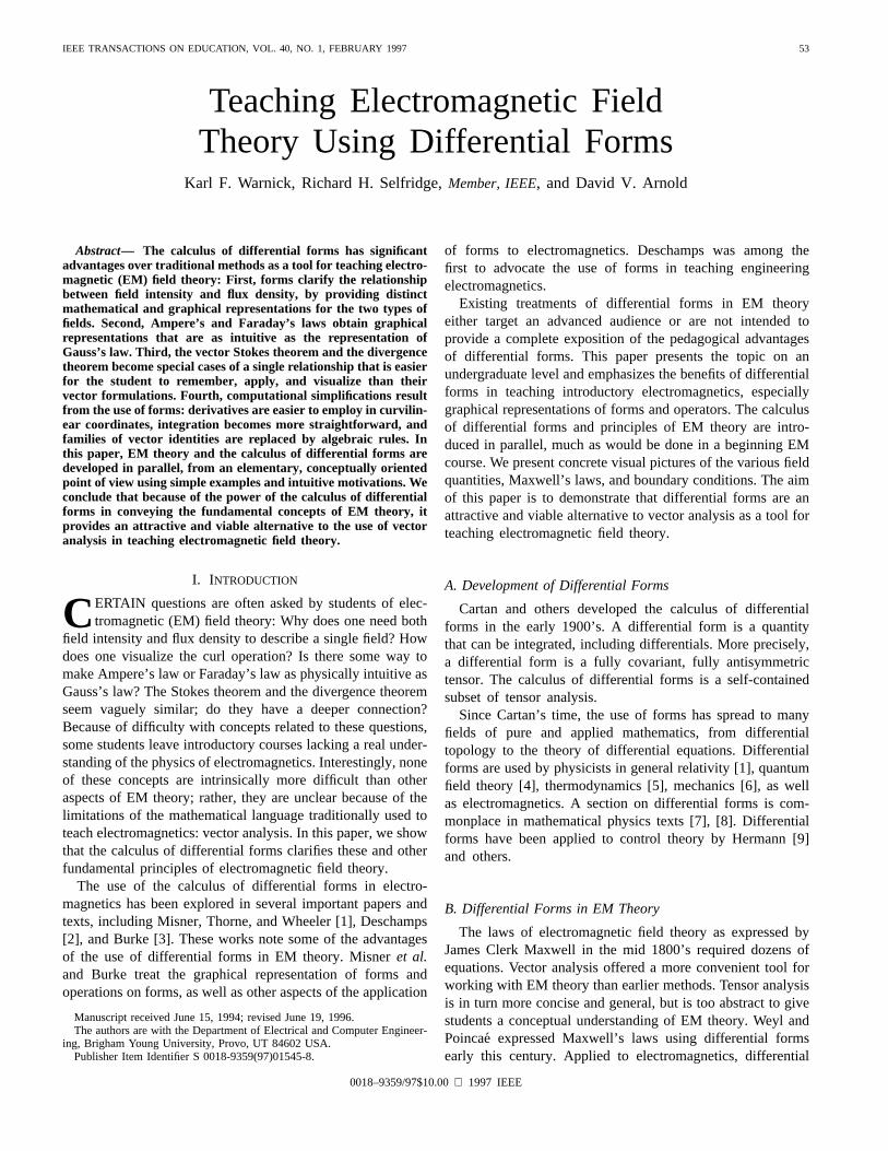
Fig. 1. (a) The1-form dx, with surfaces perpendicular to thex-axis andinfinite in the y and z directions. (b) The1-form 2 dz, with surfacesperpendicular to thez-axis and spaced two per unit distance in thez direction.(c) A general1-form, with curved surfaces and surfaces that end or meet eachother.

field. This leads naturally to the equipotential representationof the field, or the “energy picture.” The energy picture shiftsemphasis from the local concept of force experienced by atest charge to the global behavior of the field as manifestedby change in energy of a test charge as it moves along apath.

Differential forms lead to the “energy picture” of fieldintensity. A -form is represented graphically as surfacesin space [1], [3]. For a conservative field, the surfaces ofthe associated-form are equipotentials. The differentialproduces surfaces perpendicular to the-axis, as shown inFig. 1(a). Likewise, has surfaces perpendicular to the-axis and the surfaces of are perpendicular to the-axis.A linear combination of these differentials has surfaces thatare skew to the coordinate axes. The coefficients of a-form determine the spacing of the surfaces per unit length;the greater the magnitude of the coefficients, the more closelyspaced are the surfaces. The-form , shown in Fig. 1(b),has surfaces spaced twice as closely as those ofin Fig. 1(a).

In general, the surfaces of a-form can curve, end, ormeet each other, depending on the behavior of the coefficients


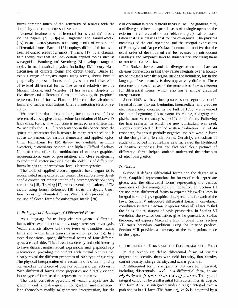
Fig. 2. A path piercing four surfaces of a 1-form. The integral of the 1-formover the path is four.

of the form. If surfaces of a -form do not meet or end,the field represented by the form is conservative. The fieldcorresponding to the-form in Fig. 1(a) is conservative; thefield in Fig. 1(c) is nonconservative.

Just as a line representing the magnitude of a vector has twopossible orientations, the surfaces of a-form are orientedas well. This is done by specifying one of the two normaldirections to the surfaces of the form. The surfaces ofare oriented in the direction, and those of in the

direction. The orientation of a form is usually clear fromcontext and is omitted from figures.

Differential forms are by definition the quantities that canbe integrated, so it is natural that the surfaces of a-form area graphical representation of path integration. The integral ofa -form along a path is the number of surfaces pierced bythe path (Fig. 2), taking into account the relative orientationsof the surfaces and the path. This simple picture of pathintegration will provide in the next section a means forvisualizing Ampere’s and Faraday’s laws.

The -form is said to bedual to thevector field . The field intensity -formsand are dual to the vectors and .

Following Deschamps, we take the units of the electric andmagnetic field intensity -forms to be volts and amperes, asshown in Table II. The differentials are considered to haveunits of length. Other field and source quantities are assignedunits according to this same convention. A disadvantage ofDeschamps’ system is that it implies in a sense that themetric of space carries units. Alternative conventions areavailable; Bamberg and Sternberg [5] and others take theunits of the electric and magnetic field intensity-forms tobe volts per meter and amperes per meter, the same as theirvector counterparts, so that the differentials carry no unitsand the integration process itself is considered to providea factor of length. If this convention is chosen, the basisdifferentials of curvilinear coordinate systems (see Section IV)must also be taken to carry no units. This leads to confusionfor students, since these basis differentials can include factorsof distance. The advantages of this alternative convention arethat it is more consistent with the mathematical point of view,in which basis vectors and forms are abstract objects notassociated with a particular system of units, and that a fieldquantity has the same units whether represented by a vectoror a differential form. Furthermore, a general differential formmay include differentials of functions that do not represent

(a) (b)

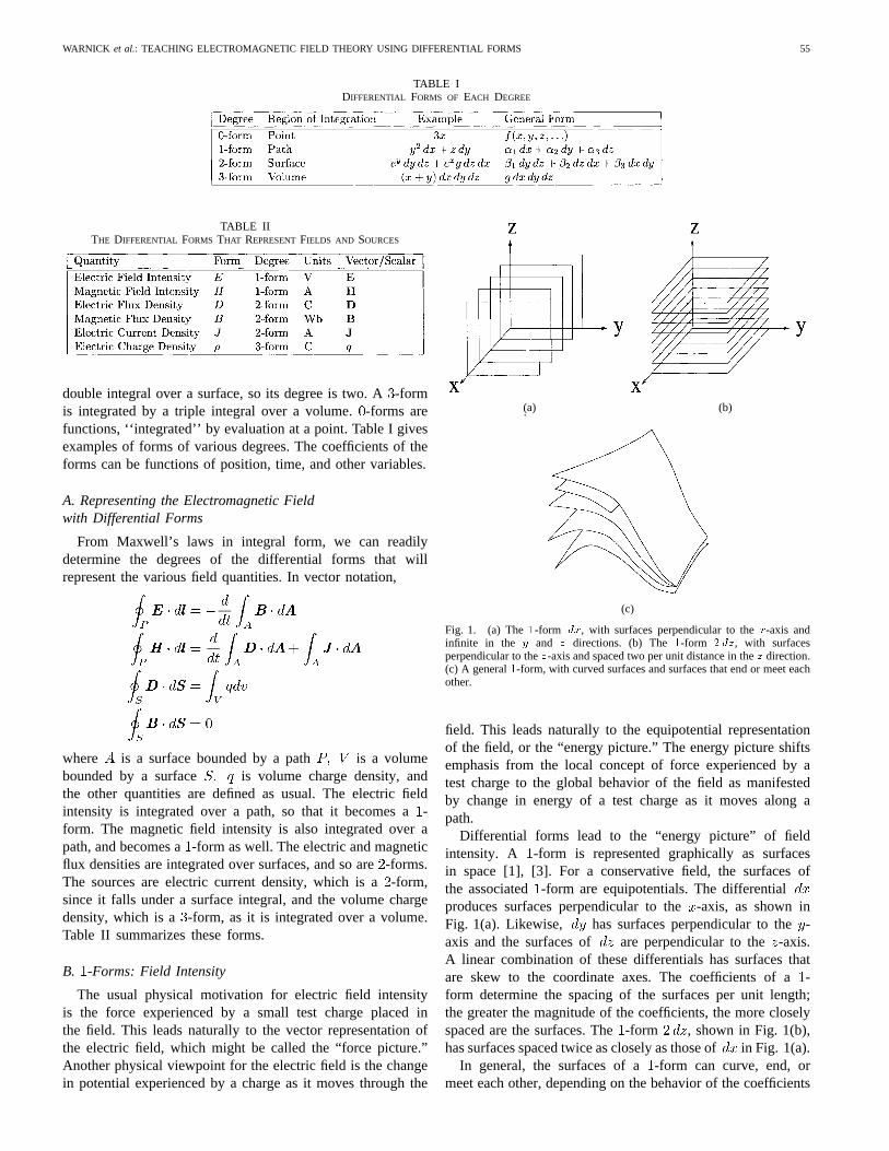
Fig. 3. (a) The2-form dx dy, with tubes in thez direction. (b) Four tubesof a 2-form pass through a surface, so that the integral of the2-form overthe surface is four.

position and so cannot be assigned units of length. Thepossibility of confusion when using curvilinear coordinatesseems to outweigh these considerations, and so we have chosenDeschamps’ convention.

With this convention, the electric field intensity-form canbe taken to have units of energy per charge, or joules percoulomb. This supports the “energy picture,” in which theelectric field represents the change in energy experienced by acharge as it moves through the field. One might argue thatthis motivation of field intensity is less intuitive than theconcept of force experienced by a test charge at a point. Whilethis may be true, the graphical representations of Ampere’sand Faraday’s laws that will be outlined in Section III favorthe differential form point of view. Furthermore, the simplecorrespondence between vectors and forms allows both to beintroduced with little additional effort, providing students amore solid understanding of field intensity than they couldobtain from one representation alone.

C. -Forms: Flux Density and Current Density

Flux density or flow of current can be thought of as tubesthat connect sources of flux or current. This is the naturalgraphical representation of a-form, which is drawn as setsof surfaces that intersect to form tubes. The differentialis represented by the surfaces of and superimposed.The surfaces of perpendicular to the -axis and those of

perpendicular to the-axis intersect to produce tubes in thedirection, as illustrated by Fig. 3(a). (To be precise, the tubes

of a -form have no definite shape: tubes of have thesame density those of .) The coefficients of a -form give the spacing of the tubes. The greater the coefficients,the more dense the tubes. An arbitrary-form has tubes thatmay curve or converge at a point.

The direction of flow or flux along the tubes of a-form isgiven by the right-hand rule applied to the orientations of thesurfaces making up the walls of a tube. The orientation ofis in the direction, and in the direction, so the fluxdue to is in the direction.

As with -forms, the graphical representation of a-form isfundamentally related to the integration process. The integralof a -form over a surface is the number of tubes passingthrough the surface, where each tube is weighted positively if


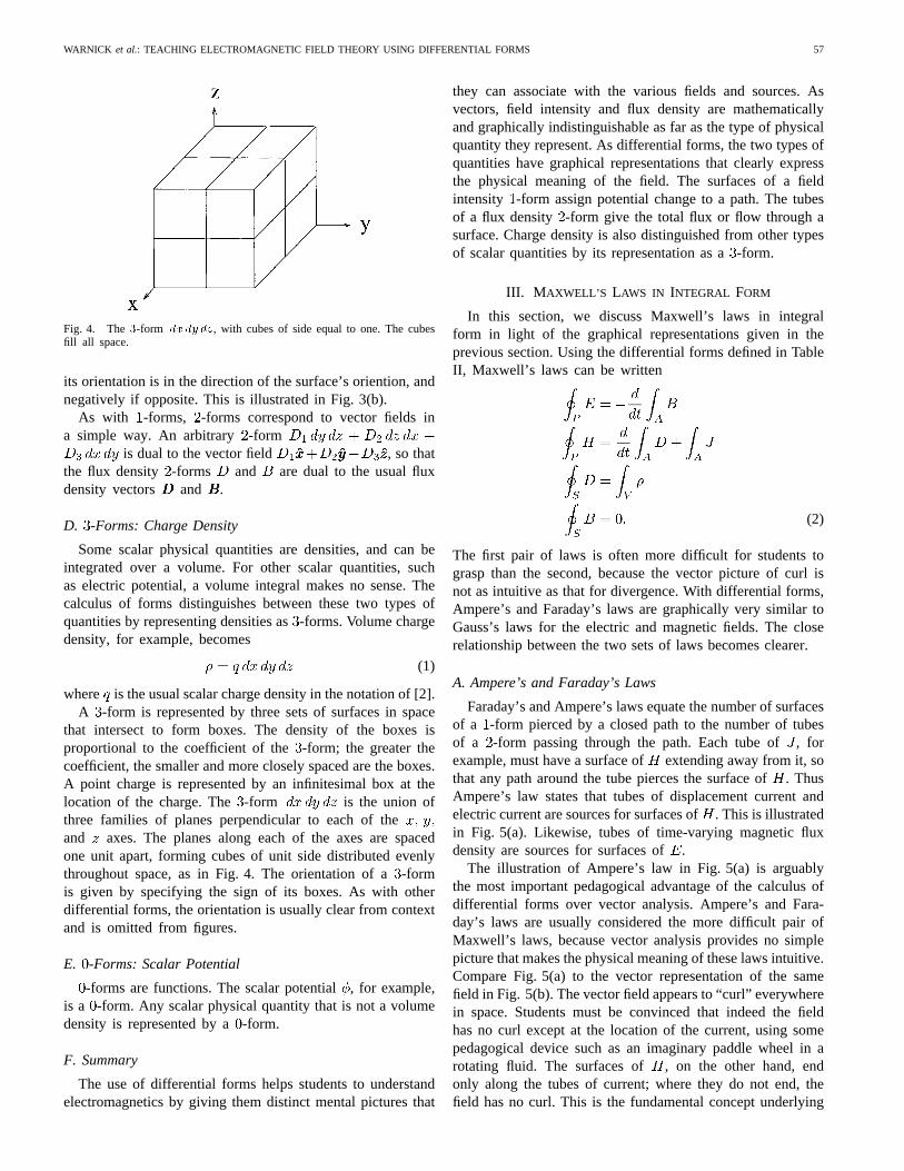
Fig. 4. The3-form dx dy dz, with cubes of side equal to one. The cubesfill all space.

its orientation is in the direction of the surface’s oriention, andnegatively if opposite. This is illustrated in Fig. 3(b).

As with -forms, -forms correspond to vector fields ina simple way. An arbitrary -form

is dual to the vector field , so thatthe flux density -forms and are dual to the usual fluxdensity vectors and .

D. -Forms: Charge Density

Some scalar physical quantities are densities, and can beintegrated over a volume. For other scalar quantities, suchas electric potential, a volume integral makes no sense. Thecalculus of forms distinguishes between these two types ofquantities by representing densities as-forms. Volume chargedensity, for example, becomes

(1)

where is the usual scalar charge density in the notation of [2].A -form is represented by three sets of surfaces in space

that intersect to form boxes. The density of the boxes isproportional to the coefficient of the-form; the greater thecoefficient, the smaller and more closely spaced are the boxes.A point charge is represented by an infinitesimal box at thelocation of the charge. The-form is the union ofthree families of planes perpendicular to each of theand axes. The planes along each of the axes are spacedone unit apart, forming cubes of unit side distributed evenlythroughout space, as in Fig. 4. The orientation of a-formis given by specifying the sign of its boxes. As with otherdifferential forms, the orientation is usually clear from contextand is omitted from figures.

E. -Forms: Scalar Potential

-forms are functions. The scalar potential, for example,is a -form. Any scalar physical quantity that is not a volumedensity is represented by a-form.

F. Summary

The use of differential forms helps students to understandelectromagnetics by giving them distinct mental pictures that

they can associate with the various fields and sources. Asvectors, field intensity and flux density are mathematicallyand graphically indistinguishable as far as the type of physicalquantity they represent. As differential forms, the two types ofquantities have graphical representations that clearly expressthe physical meaning of the field. The surfaces of a fieldintensity -form assign potential change to a path. The tubesof a flux density -form give the total flux or flow through asurface. Charge density is also distinguished from other typesof scalar quantities by its representation as a-form.

III. M AXWELL’S LAWS IN INTEGRAL FORM

In this section, we discuss Maxwell’s laws in integralform in light of the graphical representations given in theprevious section. Using the differential forms defined in TableII, Maxwell’s laws can be written

(2)

The first pair of laws is often more difficult for students tograsp than the second, because the vector picture of curl isnot as intuitive as that for divergence. With differential forms,Ampere’s and Faraday’s laws are graphically very similar toGauss’s laws for the electric and magnetic fields. The closerelationship between the two sets of laws becomes clearer.

A. Ampere’s and Faraday’s Laws

Faraday’s and Ampere’s laws equate the number of surfacesof a -form pierced by a closed path to the number of tubesof a -form passing through the path. Each tube of, forexample, must have a surface ofextending away from it, sothat any path around the tube pierces the surface of. ThusAmpere’s law states that tubes of displacement current andelectric current are sources for surfaces of. This is illustratedin Fig. 5(a). Likewise, tubes of time-varying magnetic fluxdensity are sources for surfaces of.

The illustration of Ampere’s law in Fig. 5(a) is arguablythe most important pedagogical advantage of the calculus ofdifferential forms over vector analysis. Ampere’s and Fara-day’s laws are usually considered the more difficult pair ofMaxwell’s laws, because vector analysis provides no simplepicture that makes the physical meaning of these laws intuitive.Compare Fig. 5(a) to the vector representation of the samefield in Fig. 5(b). The vector field appears to “curl” everywherein space. Students must be convinced that indeed the fieldhas no curl except at the location of the current, using somepedagogical device such as an imaginary paddle wheel in arotating fluid. The surfaces of , on the other hand, endonly along the tubes of current; where they do not end, thefield has no curl. This is the fundamental concept underlying


(a) (b)

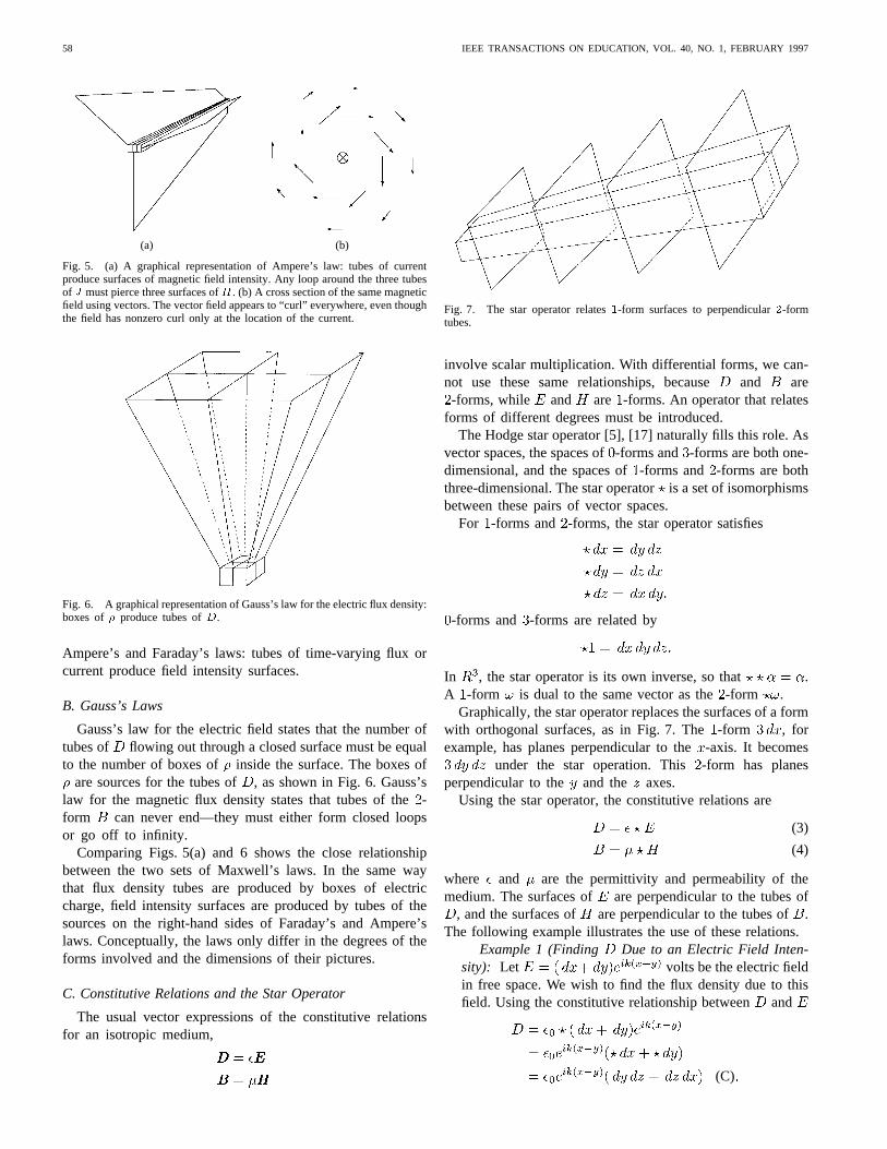
Fig. 5. (a) A graphical representation of Ampere’s law: tubes of currentproduce surfaces of magnetic field intensity. Any loop around the three tubesof J must pierce three surfaces ofH. (b) A cross section of the same magneticfield using vectors. The vector field appears to “curl” everywhere, even thoughthe field has nonzero curl only at the location of the current.

Fig. 6. A graphical representation of Gauss’s law for the electric flux density:boxes of� produce tubes ofD.

Ampere’s and Faraday’s laws: tubes of time-varying flux orcurrent produce field intensity surfaces.

B. Gauss’s Laws

Gauss’s law for the electric field states that the number oftubes of flowing out through a closed surface must be equalto the number of boxes of inside the surface. The boxes of

are sources for the tubes of, as shown in Fig. 6. Gauss’slaw for the magnetic flux density states that tubes of the-form can never end—they must either form closed loopsor go off to infinity.

Comparing Figs. 5(a) and 6 shows the close relationshipbetween the two sets of Maxwell’s laws. In the same waythat flux density tubes are produced by boxes of electriccharge, field intensity surfaces are produced by tubes of thesources on the right-hand sides of Faraday’s and Ampere’slaws. Conceptually, the laws only differ in the degrees of theforms involved and the dimensions of their pictures.

C. Constitutive Relations and the Star Operator

The usual vector expressions of the constitutive relationsfor an isotropic medium,

Fig. 7. The star operator relates1-form surfaces to perpendicular2-formtubes.

involve scalar multiplication. With differential forms, we can-not use these same relationships, becauseand are-forms, while and are -forms. An operator that relates

forms of different degrees must be introduced.The Hodge star operator [5], [17] naturally fills this role. As

vector spaces, the spaces of-forms and -forms are both one-dimensional, and the spaces of-forms and -forms are boththree-dimensional. The star operatoris a set of isomorphismsbetween these pairs of vector spaces.

For -forms and -forms, the star operator satisfies

-forms and -forms are related by

In , the star operator is its own inverse, so that .A -form is dual to the same vector as the-form .

Graphically, the star operator replaces the surfaces of a formwith orthogonal surfaces, as in Fig. 7. The-form , forexample, has planes perpendicular to the-axis. It becomes

under the star operation. This-form has planesperpendicular to the and the axes.

Using the star operator, the constitutive relations are

(3)

(4)

where and are the permittivity and permeability of themedium. The surfaces of are perpendicular to the tubes of

, and the surfaces of are perpendicular to the tubes of.The following example illustrates the use of these relations.

Example 1 (Finding Due to an Electric Field Inten-sity): Let volts be the electric fieldin free space. We wish to find the flux density due to thisfield. Using the constitutive relationship betweenand

(C)


While we restrict our attention to isotropic media in thispaper, the star operator applies equally well to anisotropicmedia. As discussed in [5] and elsewhere, the star operatordepends on a metric. If the metric is related to the permittivityor the permeability tensor, anisotropic star operators are ob-tained, and the constitutive relations become and

[20]. Graphically, an anisotropic star operator actson -form surfaces to produce-form tubes that intersect thesurfaces obliquely rather than orthogonally.

D. The Exterior Product and the Poynting-form

Between the differentials of -forms and -forms is animplied exterior product, denoted by a wedge. The wedgeis nearly always omitted from the differentials of a form,especially when the form appears under an integral sign.The exterior product of -forms is anticommutative, so that

. As a consequence, the exterior productis in general supercommutative, so that

(5)

where and are the degrees of and , respectively. Oneusually converts the differentials of a form to right-cyclic orderusing (5).

As a consequence of (5), any differential form with a re-peated differential vanishes. In a three-dimensional space eachterm of a -form will always contain a repeated differential if

, so there are no nonzero-forms for .The exterior product of two -forms is analogous to the

vector cross product. With vector analysis, it is not obviousthat the cross product of vectors is a different type of quantitythan the factors. Under coordinate inversion, changessign relative to a vector with the same components, so that

is a pseudovector. With forms, the distinction betweenand or individually is clear.

The exterior product of a-form and a -form correspondsto the dot product. The coefficient of the resulting-form isequal to the dot product of the vector fields dual to the-formand -form in the Euclidean metric.

Combinations of cross and dot products are somewhatdifficult to manipulate algebraically, often requiring the useof tabulated identities. Using the supercommutativity of theexterior product, the student can easily manipulate arbitraryproducts of forms. For example, the identities

are special cases of

where and are forms of arbitrary degrees. The factorscan be interchanged easily using (5).

Fig. 8. The Poynting power flow2-form S = E ^ H. Surfaces of the1-formsE andH are the sides of the tubes ofS.

Consider the exterior product of the 1-formsand

This is the Poynting -form . For complex fields,. For time-varying fields, the tubes of this-form

represent flow of electromagnetic power, as shown in Fig. 8.The sides of the tubes are the surfaces ofand . This gives aclear geometrical interpretation to the fact that the direction ofpower flow is orthogonal to the orientations of bothand .

Example 2 (The Poynting-Form Due to a Plane Wave):Consider a plane wave propagating in free space in thedirection, with the time-harmonic electric fieldvolts in the direction. The Poynting -form is

(W)

where is the wave impedance of free space.

E. Energy Density

The exterior products and are -forms thatrepresent the density of electromagnetic energy. The energydensity -form is defined to be

(6)

The volume integral of gives the total energy stored in aregion of space by the fields present in the region.

Fig. 9 shows the energy density-form between the platesof a capacitor, where the upper and lower plates are equally


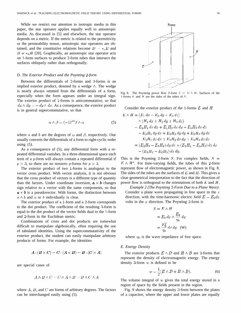
Fig. 9. The3-form 2w due to fields inside a parallel-plate capacitor withoppositely charged plates. The surfaces ofE are parallel to the top and bottomplates. The tubes ofD extend vertically from charges on one plate to oppositecharges on the other. The tubes and surfaces intersect to form cubes of2!,one of which is outlined in the figure.

and oppositely charged. The boxes of are the intersectionof the surfaces of , which are parallel to the plates, with thetubes of , which extend vertically from one plate to the other.

IV. CURVILINEAR COORDINATE SYSTEMS

In this section, we give the basis differentials, the star op-erator, and the correspondence between vectors and forms forcylindrical, spherical, and generalized orthogonal coordinates.

A. Cylindrical Coordinates

The differentials of the cylindrical coordinate system are, , and . Each of the basis differentials is considered

to have units of length. The general-form

(7)

is dual to the vector

(8)

The general -form

(9)

is dual to the same vector. The-form , for example,is dual to the vector .

Differentials must be converted to basis elements beforethe star operator is applied. The star operator in cylindricalcoordinates acts as follows:

Also, . As with the rectangular coordinatesystem, . The star operator applied to , forexample, yields .

Fig. 10 shows the pictures of the differentials of the cylin-drical coordinate system. The-forms can be obtained bysuperimposing these surfaces. Tubes of , for example,are square rings formed by the union of Figs. 10(a) and 10(c).

(a) (b)

(c)

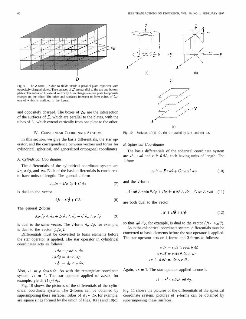
Fig. 10. Surfaces of (a)d�, (b) d� scaled by3=�, and (c) dz.

B. Spherical Coordinates

The basis differentials of the spherical coordinate systemare and , each having units of length. The-form

(10)

and the -form

(11)

are both dual to the vector

(12)

so that , for example, is dual to the vector .As in the cylindrical coordinate system, differentials must be

converted to basis elements before the star operator is applied.The star operator acts on-forms and -forms as follows:

Again, . The star operator applied to one is

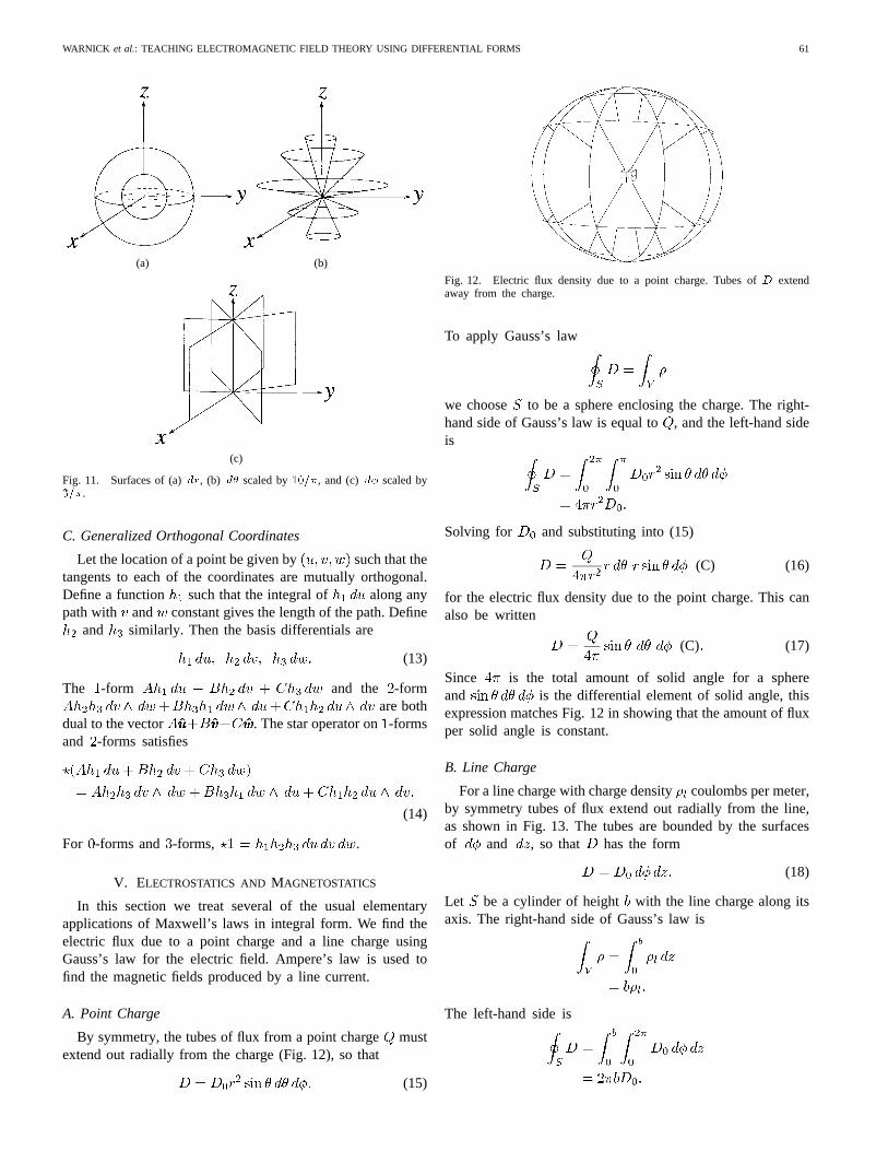
Fig. 11 shows the pictures of the differentials of the sphericalcoordinate system; pictures of-forms can be obtained bysuperimposing these surfaces.


(a) (b)

(c)

Fig. 11. Surfaces of (a)dr, (b) d� scaled by10=�, and (c) d� scaled by3=�.

C. Generalized Orthogonal Coordinates

Let the location of a point be given by such that thetangents to each of the coordinates are mutually orthogonal.Define a function such that the integral of along anypath with and constant gives the length of the path. Define

and similarly. Then the basis differentials are

(13)

The -form and the -formare both

dual to the vector . The star operator on-formsand -forms satisfies

(14)

For -forms and -forms, .

V. ELECTROSTATICS AND MAGNETOSTATICS

In this section we treat several of the usual elementaryapplications of Maxwell’s laws in integral form. We find theelectric flux due to a point charge and a line charge usingGauss’s law for the electric field. Ampere’s law is used tofind the magnetic fields produced by a line current.

A. Point Charge

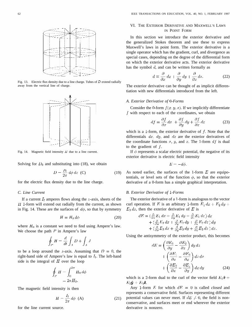
By symmetry, the tubes of flux from a point chargemustextend out radially from the charge (Fig. 12), so that

(15)

Fig. 12. Electric flux density due to a point charge. Tubes ofD extendaway from the charge.

To apply Gauss’s law

we choose to be a sphere enclosing the charge. The right-hand side of Gauss’s law is equal to, and the left-hand sideis

Solving for and substituting into (15)

(C) (16)

for the electric flux density due to the point charge. This canalso be written

(C) (17)

Since is the total amount of solid angle for a sphereand is the differential element of solid angle, thisexpression matches Fig. 12 in showing that the amount of fluxper solid angle is constant.

B. Line Charge

For a line charge with charge densitycoulombs per meter,by symmetry tubes of flux extend out radially from the line,as shown in Fig. 13. The tubes are bounded by the surfacesof and , so that has the form

(18)

Let be a cylinder of height with the line charge along itsaxis. The right-hand side of Gauss’s law is

The left-hand side is


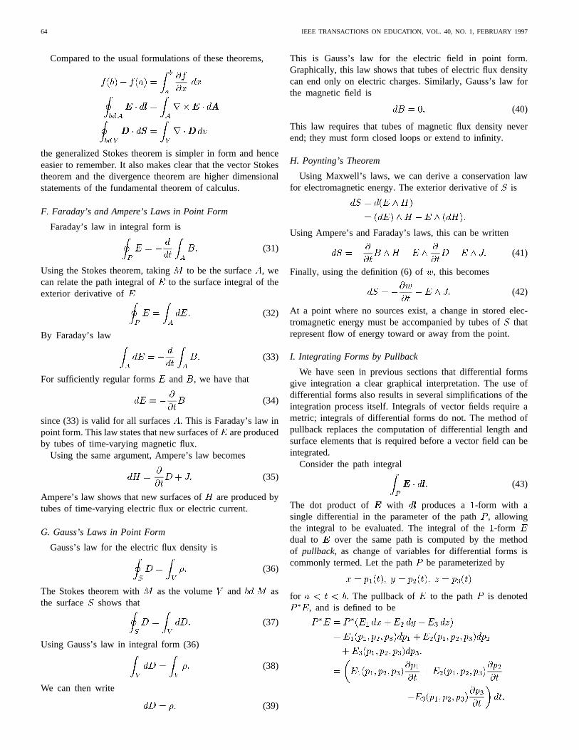
Fig. 13. Electric flux density due to a line charge. Tubes ofD extend radiallyaway from the vertical line of charge.

Fig. 14. Magnetic field intensityH due to a line current.

Solving for and substituting into (18), we obtain

(C) (19)

for the electric flux density due to the line charge.

C. Line Current

If a current amperes flows along the-axis, sheets of the-form will extend out radially from the current, as shown

in Fig. 14. These are the surfaces of, so that by symmetry

(20)

where is a constant we need to find using Ampere’s law.We choose the path in Ampere’s law

to be a loop around the-axis. Assuming that , theright-hand side of Ampere’s law is equal to. The left-handside is the integral of over the loop

The magnetic field intensity is then

(A) (21)

for the line current source.

VI. THE EXTERIOR DERIVATIVE AND MAXWELL’S LAWS

IN POINT FORM

In this section we introduce the exterior derivative andthe generalized Stokes theorem and use these to expressMaxwell’s laws in point form. The exterior derivative is asingle operator which has the gradient, curl, and divergence asspecial cases, depending on the degree of the differential formon which the exterior derivative acts. The exterior derivativehas the symbol , and can be written formally as

(22)

The exterior derivative can be thought of as implicit differen-tiation with new differentials introduced from the left.

A. Exterior Derivative of -Forms

Consider the -form . If we implicitly differentiatewith respect to each of the coordinates, we obtain

(23)

which is a -form, the exterior derivative of . Note that thedifferentials and are the exterior derivatives ofthe coordinate functions and . The -form is dualto the gradient of .

If represents a scalar electric potential, the negative of itsexterior derivative is electric field intensity

As noted earlier, the surfaces of the 1-form are equipo-tentials, or level sets of the function, so that the exteriorderivative of a 0-form has a simple graphical interpretation.

B. Exterior Derivative of -Forms

The exterior derivative of a-form is analogous to the vectorcurl operation. If is an arbitrary -form

, then the exterior derivative of is

Using the antisymmetry of the exterior product, this becomes

(24)

which is a -form dual to the curl of the vector field.

Any -form for which is called closed andrepresents a conservative field. Surfaces representing differentpotential values can never meet. If , the field is non-conservative, and surfaces meet or end wherever the exteriorderivative is nonzero.


C. Exterior Derivative of -Forms

The exterior derivative of a-form is computed by the samerule as for -forms and -forms: take partial derivatives byeach coordinate variable and add the corresponding differentialon the left. For an arbitrary-form

where six of the terms vanish due to repeated differentials.The coefficient of the resulting-form is the divergence of thevector field dual to .

D. Properties of the Exterior Derivative

Because the exterior derivative unifies the gradient, curl, anddivergence operators, many common vector identities becomespecial cases of simple properties of the exterior derivative.The equality of mixed partial derivatives leads to the identity

(25)

so that the exterior derivative applied twice yields zero.This relationship is equivalent to the vector relationships

and . The exterior derivativealso obeys the product rule

(26)

where is the degree of . A special case of (26) is

These and other vector identities are often placed in referencetables; by contrast, (25) and (26) are easily remembered.

The exterior derivative in cylindrical coordinates is

(27)

which is the same as for rectangular coordinates but with thecoordinates in the place of . Note that the exteriorderivative does not require the factor ofthat is involved inconverting forms to vectors and applying the star operator. Inspherical coordinates

(28)

where the factors and are not found in the exteriorderivative operator. The exterior derivative is

(29)

in general orthogonal coordinates. The exterior derivative ismuch easier to apply in curvilinear coordinates than the vectorderivatives; there is no need for reference tables of derivativeformulas in various coordinate systems.

(a) (b)

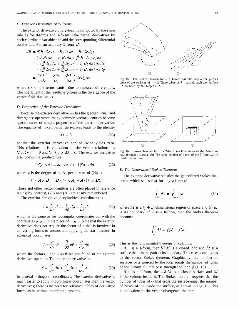
Fig. 15. The Stokes theorem for! a 1-form. (a) The loopbdM piercesthree of the surfaces of!. (b) Three tubes ofd! pass through any surfaceM bounded by the loopbdM .

(a) (b)

Fig. 16. Stokes theorem for! a 2-form. (a) Four tubes of the2-form !

pass through a surface. (b) The same number of boxes of the3-form d! lieinside the surface.

E. The Generalized Stokes Theorem

The exterior derivative satisfies the generalized Stokes the-orem, which states that for any-form

(30)

where is a -dimensional region of space andis its boundary. If is a -form, then the Stokes theorembecomes

This is the fundamental theorem of calculus.If is a -form, then is a closed loop and is a

surface that has the path as its boundary. This case is analogousto the vector Stokes theorem. Graphically, the number ofsurfaces of pierced by the loop equals the number of tubesof the -form that pass through the loop (Fig. 15).

If is a -form, then is a closed surface andis the volume inside it. The Stokes theorem requires that thenumber of tubes of that cross the surface equal the numberof boxes of inside the surface, as shown in Fig. 16. Thisis equivalent to the vector divergence theorem.


Compared to the usual formulations of these theorems,

the generalized Stokes theorem is simpler in form and henceeasier to remember. It also makes clear that the vector Stokestheorem and the divergence theorem are higher dimensionalstatements of the fundamental theorem of calculus.

F. Faraday’s and Ampere’s Laws in Point Form

Faraday’s law in integral form is

(31)

Using the Stokes theorem, taking to be the surface , wecan relate the path integral of to the surface integral of theexterior derivative of

(32)

By Faraday’s law

(33)

For sufficiently regular forms and , we have that

(34)

since (33) is valid for all surfaces. This is Faraday’s law inpoint form. This law states that new surfaces ofare producedby tubes of time-varying magnetic flux.

Using the same argument, Ampere’s law becomes

(35)

Ampere’s law shows that new surfaces ofare produced bytubes of time-varying electric flux or electric current.

G. Gauss’s Laws in Point Form

Gauss’s law for the electric flux density is

(36)

The Stokes theorem with as the volume and asthe surface shows that

(37)

Using Gauss’s law in integral form (36)

(38)

We can then write

(39)

This is Gauss’s law for the electric field in point form.Graphically, this law shows that tubes of electric flux densitycan end only on electric charges. Similarly, Gauss’s law forthe magnetic field is

(40)

This law requires that tubes of magnetic flux density neverend; they must form closed loops or extend to infinity.

H. Poynting’s Theorem

Using Maxwell’s laws, we can derive a conservation lawfor electromagnetic energy. The exterior derivative ofis

Using Ampere’s and Faraday’s laws, this can be written

(41)

Finally, using the definition (6) of , this becomes

(42)

At a point where no sources exist, a change in stored elec-tromagnetic energy must be accompanied by tubes ofthatrepresent flow of energy toward or away from the point.

I. Integrating Forms by Pullback

We have seen in previous sections that differential formsgive integration a clear graphical interpretation. The use ofdifferential forms also results in several simplifications of theintegration process itself. Integrals of vector fields require ametric; integrals of differential forms do not. The method ofpullback replaces the computation of differential length andsurface elements that is required before a vector field can beintegrated.

Consider the path integral

(43)

The dot product of with produces a -form with asingle differential in the parameter of the path, allowingthe integral to be evaluated. The integral of the-formdual to over the same path is computed by the methodof pullback, as change of variables for differential forms iscommonly termed. Let the path be parameterized by

for . The pullback of to the path is denoted, and is defined to be


Using the pullback of , we convert the integral over to anintegral in over the interval

(44)

Components of the Jacobian matrix of the coordinate transformfrom the original coordinate system to the parameterizationof the region of integration enter naturally when the exteriorderivatives are performed. Pullback works similarly for-forms and -forms, allowing evaluation of surface and volumeintegrals by the same method. The following example illus-trates the use of pullback.

Example 3 (Work Required to Move a Charge throughan Electric Field): Let the electric field intensity be givenby . A charge of istransported over the path given by

from to . The work required is given by

(45)

which by (44) is equal to

where is the pullback of the field-form to the path

Integrating this new -form in over , we obtain

as the total work required to move the charge along.

J. Existence of Graphical Representations

With the exterior derivative, a condition can be given for theexistence of the graphical representations of Section II. Theserepresentations do not correspond to the usual “tangent space”picture of a vector field, but rather are analogous to the integralcurves of a vector field. Obtaining the graphical representationof a differential form as a family of surfaces is the generalnontrivial, and is essentially equivalent to Pfaff’s problem. Bythe solution of Pfaff’s problem, each differential form may berepresented graphically in two dimensions as families of lines.In three dimensions, a-form can be represented as surfacesif the rotation is zero. If , then there existlocal coordinates for which has the form , so thatit is the sum of two -forms, both of which can be graphicallyrepresented as surfaces. An arbitrary, smooth-form incan be written locally in the form , so that the -formconsists of tubes of scaled by .

K. Summary

Throughout this section, we have noted various aspects ofthe calculus of differential forms that simplify manipulationsand provide insight into the principles of electromagnetics. Theexterior derivative behaves differently depending on the degreeof the form it operates on, so that physical properties of a fieldare encoded in the type of form used to represent it, ratherthan in the type of operator used to take its derivative. Thegeneralized Stokes theorem gives the vector Stokes theoremand the divergence theorem intuitive graphical interpretationsthat illuminate the relationship between the two theorems.While of lesser pedagogical importance, the algebraic andcomputational advantages of forms cited in this section alsoaid students by reducing the need for reference tables ormemorization of identities.

VII. T HE INTERIOR PRODUCT AND BOUNDARY CONDITIONS

Boundary conditions can be expressed using a combinationof the exterior and interior products. The same operator isused to express boundary conditions for field intensities andflux densities, and in both cases the boundary conditions havesimple graphical interpretations.

A. The Interior Product

The interior product has the symbol. Graphically, theinterior product removes the surfaces of the first form fromthose of the second. The interior product , sincethere are no surfaces to remove. The interior product of

with itself is one. The interior product of and is. To compute the interior product ,

the differential must be moved to the left of beforeit can be removed, so that

The interior product of arbitrary 1-forms can be found bylinearity from the relationships

(46)

The interior product of a 1-form and a 2-form can be foundusing

(47)

The following examples illustrate the use of the interiorproduct.


Example 4 (The Interior Product of Two 1-Forms):Theinterior product of and is

which is the dot product of the vectors dual to the-forms and .

Example 5 (The Interior Product of a-Form and a-Form): The interior product of and

is

which is the -form dual to , where and are dualto and .The interior product can be related to the exterior product

using the star operator. The interior product of arbitrary formsand is

(48)

which can be used to compute the interior product in curvi-linear coordinate systems. (This formula shows the metricdependence of the interior product as we have defined it; theinterior product is usually defined to be the contraction of avector with a form, which is independent of any metric.) Theinterior and exterior products satisfy the identity

(49)

where is an arbitrary form.The Lorentz force law can be expressed using the interior

product. The force -form is

(50)

where is the velocity of a charge, and the interior productcan be computed by finding the-form dual to and usingthe rules given above. is dual to the usual force vector.The force -form has units of energy, and does not have asclear a physical interpretation as the usual force vector. In thiscase we prefer to work with the vector dual to, rather than

itself. Force, like displacement and velocity, is naturally avector quantity.

B. Boundary Conditions

A boundary can be specified as the set of points satisfyingfor some suitable function. The surface nor-

mal -form is defined to be the normalized exterior derivativeof

(51)

The surfaces of are parallel to the boundary. Using asubscript to denote the region where , and a subscript

(a) (b)

(c)

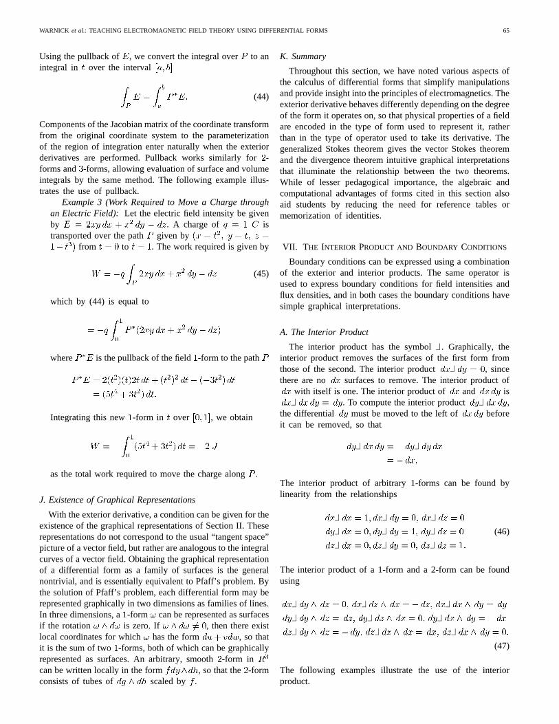
Fig. 17. (a) The1-formH1�H2. (b) The2-form n^ (H1�H2). (c) The1-formJs, represented by lines on the boundary. Current flows along the lines.

for , the four electromagnetic boundary conditions canbe written [18]

where is the surface current density-form and is thesurface charge density-form. The operator projectsan arbitrary form to its component that has nonzero integralalong the boundary.

C. Surface Current

The action of the operator can be interpreted graphi-cally, leading to a simple picture of the field intensity boundaryconditions. Consider the field discontinuity shownin Fig. 17(a). The exterior product of and isa -form with tubes that run parallel to the boundary, asshown in Fig. 17(b). The component of with surfacesparallel to the boundary is removed. The interior product

removes the surfaces parallel to theboundary, leaving only surfaces perpendicular to the boundary,as in Fig. 17(c). Current flows along the lines where thesurfaces intersect the boundary. The direction of flow alongthe lines of the -form can be found using the right-hand ruleon the direction of in region above the boundary.

The field intensity boundary conditions state that surfacesof the -form end along lines of the surface currentdensity -form . Surfaces of cannot intersect aboundary at all.

Unlike other electromagnetic quantities, is not dual tothe vector . The direction of is parallel to the linesof in the boundary, as shown in Fig. 17(c). ( is atwisted differential form, so that under coordinate inversionit transforms with a minus sign relative to a nontwisted

-form. This property is discussed in detail in [3], [18],[21]. Operationally, the distinction can be ignored as longas one remains in right-handed coordinates.) is naturalboth mathematically and geometrically as a representation of


surface current density. The expression for current through apath using the vector surface current density is

(52)

where is a surface normal. This simplifies to

(53)

using the -form . Note that changes sign dependingon the labeling of regions one and two; this ambiguity isequivalent to the existence of two choices forin (52).

The following example illustrates the boundary conditionon the magnetic field intensity.

Example 6 (Surface Current on a Sinusoidal Surface):Asinusoidal boundary given by has magneticfield intensity A above and zero below. Thesurface normal -form is

By the boundary conditions given above

(A)

The usual surface current density vector is, which clearly is not dual to .

The direction of the vector is parallel to the lines ofon the boundary.

D. Surface Charge

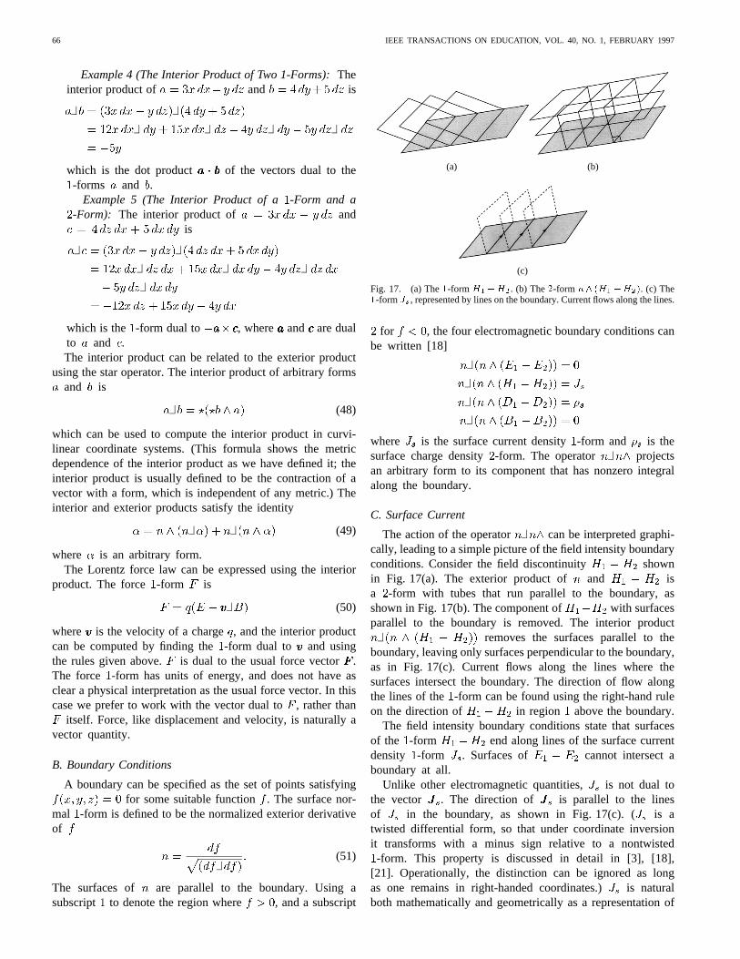
The flux density boundary conditions can also be interpretedgraphically. Fig. 18(a) shows the-form . The exteriorproduct yields boxes that have sides parallelto the boundary, as shown in Fig. 18(b). The component of

with tubes parallel to the boundary is removed bythe exterior product. The interior product withremoves thesurfaces parallel to the boundary, leaving tubes perpendicularto the boundary. These tubes intersect the boundary to formboxes of charge (Fig. 18(c)). This is the-form

.The flux density boundary conditions have as clear a graph-

ical interpretation as those for field intensity: tubes of thedifference in electric flux densities on either sideof a boundary intersect the boundary to form boxes of surfacecharge density. Tubes of the discontinuity in magnetic fluxdensity cannot intersect the boundary.

The sign of the charge on the boundary can be obtained fromthe direction of in region above the boundary, whichmust point away from positive charge and toward negativecharge. The integral of over a surface

(54)

(a) (b)

(c)

Fig. 18. (a) The2-form D1 �D2. (b) The3-form n ^ (D1 �D2), withsides perpendicular to the boundary. (c) The2-form �s, represented by boxeson the boundary.

yields the total charge on the surface. Note thatchangessign depending on the labeling of regions one and two. Thisambiguity is equivalent to the existence of two choices forthe area element and orientation of the area in theintegral , where is the usual scalar surface chargedensity. Often, the sign of the value of the integral is knownbeforehand, and this subtlety goes unnoticed.

VIII. C ONCLUSION

The primary pedagogical advantages of differential formsare the distinct representations of field intensity and flux den-sity, intuitive graphical representations of each of Maxwell’slaws, and a simple picture of electromagnetic boundary con-ditions. Differential forms provide visual models that canhelp students remember and apply the principles of electro-magnetics. Computational simplifications also result from theuse of forms: derivatives are easier to employ in curvilinearcoordinates, integration becomes more straightforward, andfamilies of related vector identities are replaced by algebraicrules. These advantages over traditional methods make thecalculus of differential forms ideal as a language for teachingelectromagnetic field theory.

The reader will note that we have omitted important aspectsof forms. In particular, we have not discussed forms as linearoperators on vectors, or covectors, focusing instead on theintegral point of view. Other aspects of electromagnetics,including vector potentials, Green functions, and wave propa-gation also benefit from the use of differential forms.

Ideally, the electromagnetics curriculum set forth in thispaper would be taught in conjunction with calculus coursesemploying differential forms. A unified curriculum, althoughdesirable, is not necessary in order for students to profit fromthe use of differential forms. We have found that becauseof the simple correspondence between vectors and forms,the transition from vector analysis to differential forms isgenerally quite easy for students to make. Familiarity withvector analysis also helps students to recognize and appreciate


the advantages of the calculus of differential forms over othermethods.

We hope that this attempt at making differential formsaccessible at the undergraduate level helps to fulfill the visionexpressed by Deschamps [2] and others, that students obtainthe power, insight, and clarity that differential forms offer toelectromagnetic field theory and its applications.

REFERENCES

[1] C. Misner, K. Thorne, and J. A. Wheeler,Gravitation. San Francisco,CA: Freeman, 1973.

[2] G. A. Deschamps, “Electromagnetics and differential forms,”Proc.IEEE, vol. 69, no. 6, pp. 676–696, June 1981.

[3] W. L. Burke, Applied Differential Geometry. Cambridge, U.K.: Cam-bridge Univ. Press, 1985.

[4] C. Nash and S. Sen,Topology and Geometry for Pphysicists. SanDiego, CA: Academic Press, 1983.

[5] P. Bamberg and S. Sternberg,A Course in Mathematics for Students ofPhysics, vol. II. Cambridge, U.K.: Cambridge Univ. Press, 1988.

[6] H. Flanders,Differential Forms with Applications to the Physical Sci-ences. New York: Dover, 1963.

[7] Y. Choquet-Bruhat and C. DeWitt-Morette,Analysis, Manifolds andPhysics. Amsterdam, The Netherlands: North-Holland, 1982.

[8] S. Hassani,Foundations of Mathematical Physics. Boston, MA: Allynand Bacon, 1991.

[9] R. Hermann,Topics in the Geometric Theory of Linear Systems. Brook-line, MA: Math Sci. Press, 1984.

[10] D. Baldomir, “Differential forms and electromagnetism in 3-dimensionalEuclidean spaceR3,” Proc. Inst. Elec. Eng., vol. 133, no. 3, pp.139–143, May 1986.

[11] N. Schleifer, “Differential forms as a basis for vector analysis-withapplications to electrodynamics,”Amer. J. Phys., vol. 51, no. 12, pp.1139–1145, Dec. 1983.

[12] D. B. Nguyen, “Relativistic constitutive relations, differential forms, andthe p-compound,”Amer. J. Phys., vol. 60, no. 12, pp. 1137–1147, Dec.1992.

[13] D. Baldomir and P. Hammond, “Global geometry of electromagneticsystems,”Proc. Inst. Elec. Eng., vol. 140, no. 2, pp. 142–150, Mar.1992.

[14] P. Hammond and D. Baldomir, “Dual energy methods in electromag-netics using tubes and slices,”Proc. Inst. Elec. Eng., vol. 135, no. 3A,pp. 167–172, Mar. 1988.

[15] R. S. Ingarden and A. Jamio lkowski, Classical Electrodynamics,. Am-sterdam, The Netherlands: Elsevier, 1985.

[16] S. Parrott, Relativistic Electrodynamics and Differential Geometry.New York: Springer-Verlag, 1987.

[17] W. Thirring, Classical Field Theory, vol. II. New York: Springer-Verlag, 1978.

[18] K. F. Warnick, R. H. Selfridge, and D. V. Arnold, “Electromagneticboundary conditions using differential forms,”Proc. Inst. Elec. Eng.,vol. 142, no. 4, pp. 326–332, 1995.

[19] K. F. Warnick and D. V. Arnold, “Electromagnetic green functions usingdifferential forms,”J. Electromagn. Waves and Appl., vol. 10, no. 3, pp.427–438, 1996.

[20] , “Differential forms in electromagnetic field theory,” inAntennasand Propagation Symp. Proc., to be published, 1996.

[21] W. L. Burke, “Manifestly parity invariant electromagnetic theory andtwisted tensors,”J. Math. Phys., vol. 24, no. 1, pp. 65–69, Jan. 1983.

Karl F. Warnick is a National Science Foundation Graduate Fellow inElectrical Engineering at Brigham Young University, Provo, UT.

His current interests include nonlinear differential equations, differentialgeometry, topology, and electromagnetics in anisotropic media.

Richard H. Selfridge (M’87) received the B.S. degree in physics fromCalifornia State University, Sacramento, in 1987, and the M.S. and Ph.D.degrees in electrical engineering from the University of California, Davis, in1980 and 1984, respectively.

From 1983 to 1987, he taught in the Department of Electrical and ComputerEngineering at California State University, Sacramento. Since July of 1987, hehas been a Professor of Electrical Engineering at Brigham Young University,Provo, UT. His research interests include modeling of conduction processesin semiconductors and mode locking of argon and dye lasers. Recently, hisresearch has been directed toward the invention and fabrication of novel D-fiber devices. In addition, he is experimenting with approaches for teachingand using differential forms in electrical engineering.

Dr. Selfridge is a member of Sigma Xi and SPIE.

David V. Arnold received the B.S. and M.S. degrees from Brigham YoungUniversity, Provo, UT, and the Ph.D. degree from the Massachusetts Instituteof Technology, Cambridge.

He is currently an Assistant Professor in the Electrical and ComputerEngineering Department at Brigham Young University. His research interestsare in electromagnetic theory and microwave remote sensing.

Teaching Electromagnetic Field Theory Using Differential ... · Teaching Electromagnetic Field...

Documents

Transcript of Teaching Electromagnetic Field Theory Using Differential ... · Teaching Electromagnetic Field...