TCP with header checksum option for wireless links: An analytical approach towards performance...
23
S¯ adhan¯ a Vol. 32, Part 3, June 2007, pp. 253–275. © Printed in India TCP with header checksum option for wireless links: An analytical approach towards performance evaluation PAWAN KUMAR GUPTA and JOY KURI Centre for Electronics Design and Technology, Indian Institute of Science, Bangalore 560 012 e-mail: [email protected], [email protected] MS received 9 June 2004; revised 26 May 2006 Abstract. TCP performs poorly in wireless mobile networks due to large bit error rates. Basically, the TCP sender responds to these losses as if they were due to congestion in the network, and reduces the congestion window unnecessarily. In earlier work, it has been shown that adding a TCP header checksum is very useful in differentiating between congestion loss and corruption loss. With the modified TCP, receivers can explicitly indicate corruption of received packets by generating “Explicit Loss Notifications (ELNs).” This paper focuses on an analytical study of this modified TCP protocol. We derive an expression for the probability of a receiver generating successful ELN, assuming a generic link layer protocol for data transfer over wireless links. Next, we develop an analytical approach for TCP throughput evaluation under the modified scheme. We compare the throughput results obtained by analysis and simulation, and find very close agreement between the two sets. We also compare the performance of the modified scheme with the standard NewReno TCP, and find considerable improvement in data throughput over wireless links. Keywords. ELN; NewReno; NewRenoEln; TCP; throughput; wireless links. 1. Introduction Transmission Control Protocol (TCP) is a reliable, end-to-end, transport protocol widely used to access the Internet and to support applications like telnet, ftp and http (Stevens 1994, Postel). TCP was designed for wired networks, where packet losses are mainly due to congestion. In today’s world, more and more people use their mobile devices to access the Internet either for work or entertainment, where TCP runs over wireless links and is subjected to more corruption losses as compared to congestion losses. Current TCP implementations respond to any such loss of packet in the traditional way by reducing the congestion window. This unnecessary reduction in the congestion window reduces throughput and wastes precious wireless resources. A lot of research has been done in this area, and many studies have proposed different ways of increasing throughput for TCP transmission over wireless networks (Balakrishnan et al 1997, Goff et al 2000, Chen & Lee 2000, Caceres & Iftode 1995, Sinha et al 1999, Bakshi 253
-
Upload
pawan-kumar-gupta -
Category
Documents
-
view
215 -
download
1
Transcript of TCP with header checksum option for wireless links: An analytical approach towards performance...
Sadhana Vol. 32, Part 3, June 2007, pp. 253–275. © Printed in India
TCP with header checksum option for wireless links: Ananalytical approach towards performance evaluation
PAWAN KUMAR GUPTA and JOY KURI
Centre for Electronics Design and Technology, Indian Institute of Science,Bangalore 560 012e-mail: [email protected], [email protected]
MS received 9 June 2004; revised 26 May 2006
Abstract. TCP performs poorly in wireless mobile networks due to large biterror rates. Basically, the TCP sender responds to these losses as if they were dueto congestion in the network, and reduces the congestion window unnecessarily. Inearlier work, it has been shown that adding a TCP header checksum is very usefulin differentiating between congestion loss and corruption loss. With the modifiedTCP, receivers can explicitly indicate corruption of received packets by generating“Explicit Loss Notifications (ELNs).” This paper focuses on an analytical study ofthis modified TCP protocol. We derive an expression for the probability of a receivergenerating successful ELN, assuming a generic link layer protocol for data transferover wireless links. Next, we develop an analytical approach for TCP throughputevaluation under the modified scheme. We compare the throughput results obtainedby analysis and simulation, and find very close agreement between the two sets. Wealso compare the performance of the modified scheme with the standard NewRenoTCP, and find considerable improvement in data throughput over wireless links.
Keywords. ELN; NewReno; NewRenoEln; TCP; throughput; wireless links.
1. Introduction
Transmission Control Protocol (TCP) is a reliable, end-to-end, transport protocol widely usedto access the Internet and to support applications like telnet, ftp and http (Stevens 1994, Postel).TCP was designed for wired networks, where packet losses are mainly due to congestion. Intoday’s world, more and more people use their mobile devices to access the Internet eitherfor work or entertainment, where TCP runs over wireless links and is subjected to morecorruption losses as compared to congestion losses. Current TCP implementations respondto any such loss of packet in the traditional way by reducing the congestion window. Thisunnecessary reduction in the congestion window reduces throughput and wastes preciouswireless resources.
A lot of research has been done in this area, and many studies have proposed different waysof increasing throughput for TCP transmission over wireless networks (Balakrishnan et al1997, Goff et al 2000, Chen & Lee 2000, Caceres & Iftode 1995, Sinha et al 1999, Bakshi
253

254 Pawan Kumar Gupta and Joy Kuri
et al 1997). These proposals mainly focus on hiding corruption losses from the TCP sender byperforming re-transmissions of any lost data to avoid coarse timeouts. Re-transmissions maybe performed either at the link level when a reliable link layer protocol is used (Balakrishnanet al 1997) or at the packet level when split connection protocol is used (Chen & Lee 2000).Balakrishnan & Katz (1998), Peng & Ma, Vaidya (1997), Parsa and Aceves (2000) havediscussed mechanisms to successfully differentiate congestion loss from corruption loss invarious scenarios. The schemes suggested in (Balakrishnan & Katz 1998, Peng & Ma) rely onintermediate nodes to provide sufficient information for distinguishing corruption loss fromcongestion loss. Such mechanisms are not useful when the IP traffic is encrypted, or whenincorporating TCP-awareness in intermediate nodes is not feasible. Vaidya (1997), Parsa &Aceves (2000) suggest the use of successive inter-arrival times of packets to heuristicallydistinguish corruption loss from congestion loss. These mechanisms work on end-to-end basisbut are not very reliable.
As shown in Balan et al (2001) and Gupta & Kuri (2002), the use of a new TCP option—the TCP header checksum option— is an attractive approach for distinguishing betweencongestion loss and corruption loss of TCP segments over wireless links. If TCP is enhanced togenerate and process this header checksum option, then explicit indications of loss on wirelesslinks can be obtained. The enhanced TCP is called “TCP HACK” in Balan et al (2001) and“TCP NewRenoELN” in Gupta & Kuri (2002)—essentially, these are identical schemes.
In this paper, we are interested in an analytical study of the proposals in Balan et al (2001)and Gupta & Kuri (2002). The first question of interest is: Given that a TCP segment is inerror, what is the probability that an “Explicit Loss Notification” (ELN) can be generated?The issue here is that a TCP segment may be fragmented into several pieces because of asmall MTU (maximum transmission unit) on the wireless link, and an unfortunate pattern oflink-level frame corruption may make it impossible for the TCP receiver to generate ELN. In§ 3, we analyse the ELN generation process and answer this question.
Secondly, we are interested in obtaining analytical expressions for the TCP throughput thatcan be achieved when the modified TCP is used. For this, we extend the analysis developedin Zorzi et al (2000) and obtain formulae for computing the throughput. Berkeley’s networksimulator ns is used to simulate the modified TCP, and the simulation results are in excellentagreement with the formulae. The analytical expressions provide a clear, quantitative pictureof the benefit that the modified TCP brings, when compared to standard NewReno TCP.
This paper is organized as follows. In § 2, we start with a brief explanation of TCP NewRenoand then describe the enhancements to TCP proposed in Balan et al (2001) and Gupta & Kuri(2002). For ease of discussion, we refer to the modified TCP proposed in Balan et al (2001)and Gupta & Kuri (2002) as “NewReno ELN”—NewReno with ELN. In § 3, we develop anexpression for the conditional probability of a receiver generating successful ELN, given thata TCP segment is received in error. In § 4, we develop a detailed analytical model for theperformance evaluation of the NewRenoELN TCP protocol. In § 5, we show that simulationresults match the analysis very closely, and also note that NewRenoELN performs appreciablybetter than NewReno.
2. The NewRenoEln TCP protocol
In this section, we start with a brief description of the TCP receiver and transmit processesspecific to NewReno, (Postel Floyd & Henderson, Kumar 1998). The TCP receiver can receivepackets out of sequence, but will only deliver them in sequence to the TCP user. The receiver
TCP with header checksum option for wireless links 255
advertises a maximum window size of Wmax, so that the transmitter does not allow more thanWmax unacknowledged packets outstanding at any given time. The receiver sends back anacknowledgement (ACK) packet for every data packet that it receives correctly. The ACKsare cumulative, i.e., an ACK carrying the acknowledgement number m acknowledges all datapackets up to, and including, the data packet with sequence number (m − 1). If a packet islost (after a stream of correctly received packets), then the transmitter keeps receiving ACKswith the sequence number of the first packet lost (called duplicate ACKs), even if the packetstransmitted after the lost packet are correctly received at the receiver.
The TCP transmitter operates on a window-based transmission strategy as follows. At anygiven time t , there is a lower window edge A(t), which means that all TCP packets numberedup to, and including, A(t)−1 have been transmitted and acknowledged, and that the transmittercan send data packets from A(t) onwards. The receipt of an ACK that acknowledges some newdata will cause an increase in A(t) by an amount equal to the amount of data acknowledged.The transmitter’s congestion window,W(t), defines the maximum amount of unacknowledgeddata packets the transmitter is permitted to send, starting from A(t). The slow start threshold,Wth(t), controls the increments in W(t). Each time a new packet is transmitted, the senderstarts a timer. If the timer reaches the round trip timeout value (derived from a round triptime estimation procedure Stevens (1994)) before the packet is acknowledged, timeout timerexpiration occurs. The evolution of W(t) and Wth(t) are triggered by ACKs and timeouts asdescribed below.
(1) If W(t) < Wth(t) (slow start phase), each ACK causes W(t) to be incremented by 1.(2) If W(t) ≥ Wth(t), each ACK causes W(t) to be incremented by 1/W(t). This is the
congestion avoidance phase.(3) If timeout occurs at the transmitter at time t , W(t+) is set to 1, Wth(t
+) is set to �W(t)/2�,and the transmitter begins retransmission from the next packet after the last acknowledgedpacket.
(4) When the K th (dupack threshold) duplicate ACK is received, Wth(t+) is set to one half
of the current “flightsize” and W(t+) is set to Wth(t+) + K . Addition of K inflates the
congestion window by the number of packets that have left the network and which thereceiver has buffered. The flightsize is defined as the number of packets that are transmittedand not yet acknowledged. The sender will also record the highest sequence numbertransmitted in the variable “recover”. The missing packet indicated by the duplicate ACKis re-transmitted at this stage. This is the fast re-transmission phase.
(5) In the fast recovery phase, each time another duplicate ACK arrives, W(t) is incrementedby one and a new packet is transmitted (if allowed by the new value of congestion window).Increment of one inflates the congestion window to reflect the additional packet that hasleft the network.
(6) When an ACK packet arrives that acknowledges all the data up to and including “recover”,then the ACK acknowledges all the intermediate packets sent between the original trans-mission of the lost packet and the receipt of the K th duplicate ACK. The congestionwindow is now set to the current value of slow start threshold, i.e., Wth(t
+). The senderexits the fast recovery phase and transmission of packets resumes in congestion avoid-ance phase.
(7) If this new ACK does not acknowledge all of the data up to and including “recover”,then this is a partial ACK. In this case, the sender re-transmits the first unacknowledgedsegment indicated by the ACK packet. It deflates the congestion window W(t) by theamount of new data acknowledged, then adds back one, and sends a new segment ifpermitted by the new value of congestion window.
256 Pawan Kumar Gupta and Joy Kuri
In the NewReno protocol, the receiver will respond in the same manner to all packet losses,which may occur either due to congestion or corruption on the wireless link. For packet lossesdue to corruption, there is no need for the TCP sender to reduce the congestion window. Thereduction in congestion window reduces the rate of flow of packets, thereby degrading thethroughput. On the other hand, if the packet loss is due to congestion, then the TCP sendershould reduce the congestion window to avoid congestion collapse in the network. Thus,an effective mechanism is required to reliably distinguish congestion losses from corruptionlosses. With the modifications suggested in Balan et al (2001) and Gupta & Kuri (2002), itis possible for the TCP sender and receiver to effectively distinguish congestion losses fromcorruption losses and take action accordingly. These modifications are described here in brief.
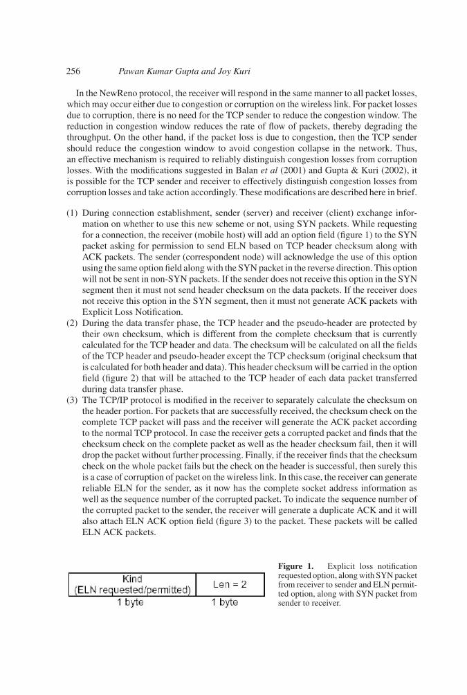
(1) During connection establishment, sender (server) and receiver (client) exchange infor-mation on whether to use this new scheme or not, using SYN packets. While requestingfor a connection, the receiver (mobile host) will add an option field (figure 1) to the SYNpacket asking for permission to send ELN based on TCP header checksum along withACK packets. The sender (correspondent node) will acknowledge the use of this optionusing the same option field along with the SYN packet in the reverse direction. This optionwill not be sent in non-SYN packets. If the sender does not receive this option in the SYNsegment then it must not send header checksum on the data packets. If the receiver doesnot receive this option in the SYN segment, then it must not generate ACK packets withExplicit Loss Notification.
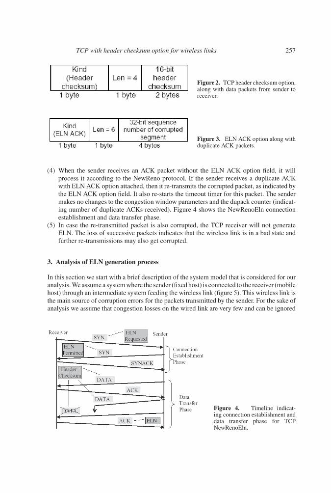
(2) During the data transfer phase, the TCP header and the pseudo-header are protected bytheir own checksum, which is different from the complete checksum that is currentlycalculated for the TCP header and data. The checksum will be calculated on all the fieldsof the TCP header and pseudo-header except the TCP checksum (original checksum thatis calculated for both header and data). This header checksum will be carried in the optionfield (figure 2) that will be attached to the TCP header of each data packet transferredduring data transfer phase.
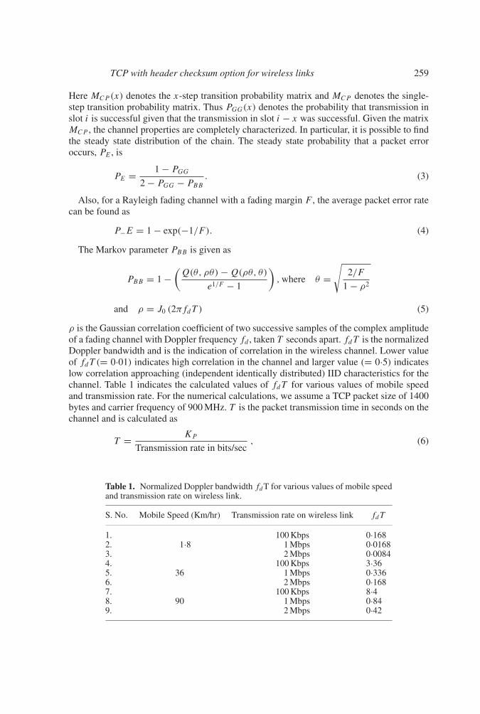
(3) The TCP/IP protocol is modified in the receiver to separately calculate the checksum onthe header portion. For packets that are successfully received, the checksum check on thecomplete TCP packet will pass and the receiver will generate the ACK packet accordingto the normal TCP protocol. In case the receiver gets a corrupted packet and finds that thechecksum check on the complete packet as well as the header checksum fail, then it willdrop the packet without further processing. Finally, if the receiver finds that the checksumcheck on the whole packet fails but the check on the header is successful, then surely thisis a case of corruption of packet on the wireless link. In this case, the receiver can generatereliable ELN for the sender, as it now has the complete socket address information aswell as the sequence number of the corrupted packet. To indicate the sequence number ofthe corrupted packet to the sender, the receiver will generate a duplicate ACK and it willalso attach ELN ACK option field (figure 3) to the packet. These packets will be calledELN ACK packets.
Figure 1. Explicit loss notificationrequested option, along with SYN packetfrom receiver to sender and ELN permit-ted option, along with SYN packet fromsender to receiver.
TCP with header checksum option for wireless links 257
Figure 2. TCP header checksum option,along with data packets from sender toreceiver.
Figure 3. ELN ACK option along withduplicate ACK packets.
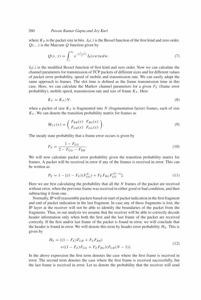
(4) When the sender receives an ACK packet without the ELN ACK option field, it willprocess it according to the NewReno protocol. If the sender receives a duplicate ACKwith ELN ACK option attached, then it re-transmits the corrupted packet, as indicated bythe ELN ACK option field. It also re-starts the timeout timer for this packet. The sendermakes no changes to the congestion window parameters and the dupack counter (indicat-ing number of duplicate ACKs received). Figure 4 shows the NewRenoEln connectionestablishment and data transfer phase.
(5) In case the re-transmitted packet is also corrupted, the TCP receiver will not generateELN. The loss of successive packets indicates that the wireless link is in a bad state andfurther re-transmissions may also get corrupted.
3. Analysis of ELN generation process
In this section we start with a brief description of the system model that is considered for ouranalysis. We assume a system where the sender (fixed host) is connected to the receiver (mobilehost) through an intermediate system feeding the wireless link (figure 5). This wireless link isthe main source of corruption errors for the packets transmitted by the sender. For the sake ofanalysis we assume that congestion losses on the wired link are very few and can be ignored
Figure 4. Timeline indicat-ing connection establishment anddata transfer phase for TCPNewRenoEln.

258 Pawan Kumar Gupta and Joy Kuri
Figure 5. Mobile host connectedto fixed host over wireless link.
when compared to wireless losses. We also assume very low bandwidth-delay product andan instantaneous and perfect feedback channel without any errors.
We assume a generic link layer protocol between intermediate system and mobile host. IPfragments the TCP packet into multiple frames depending on the wireless link’s MTU and thelink layer protocol adds some error control bits before transmitting the packet on the wirelesslink. Due to the high bit error rate on the wireless link, some of these frames are lost or arereceived in error by the receiver. Normally, the link layer protocol discards such corruptedframes and the TCP/IP layer does not receive the complete packet. We assume a modified linklayer protocol that does not discard the frames received in error. The frames received by thewireless link receiver are simply passed up to the IP layer; a corrupted frame is accompaniedby an indication that it was received in error.
We will evaluate the probability that the receiver is able to provide reliable ELN to thesender. Following Zorzi et al (1995), we model the wireless link as a discrete time Markovchain with two states: good and bad. Time is slotted in units of frame transmission time(figure 6). In § 4, figure 6 will again be used, with the modification that slot times will representpacket transmission times.
We assume that packet/frame transmission starts only at slot boundaries tk, tk+1, etc. Ifthe channel is in the good state at time t−k , then the transmission starting at time tk will besuccessful with probability 1 and when the channel is in the bad state at time t−k , then thepacket/frame transmission starting at time tk will fail with probability 1. Also, it is assumedthat the channel state changes only at the slot boundary. For such a channel the transitionprobability matrix is given by
MCP (x) =(
PBB(x) PBG(x)
PGB(x) PGG(x)
)(1)
MCP =(
PBB PBG
PGB PGG
), where MCP (x) = (MCP )x. (2)
Figure 6. Slotted timeline for packets/frames over the wireless link.
TCP with header checksum option for wireless links 259
Here MCP (x) denotes the x-step transition probability matrix and MCP denotes the single-step transition probability matrix. Thus PGG(x) denotes the probability that transmission inslot i is successful given that the transmission in slot i − x was successful. Given the matrixMCP , the channel properties are completely characterized. In particular, it is possible to findthe steady state distribution of the chain. The steady state probability that a packet erroroccurs, PE , is
PE = 1 − PGG
2 − PGG − PBB
. (3)
Also, for a Rayleigh fading channel with a fading margin F , the average packet error ratecan be found as
P−E = 1 − exp(−1/F ). (4)
The Markov parameter PBB is given as
PBB = 1 −(
Q(θ, ρθ) − Q(ρθ, θ)
e1/F − 1
), where θ =
√2/F
1 − ρ2
and ρ = J0 (2πfdT ) (5)
ρ is the Gaussian correlation coefficient of two successive samples of the complex amplitudeof a fading channel with Doppler frequency fd , taken T seconds apart. fdT is the normalizedDoppler bandwidth and is the indication of correlation in the wireless channel. Lower valueof fdT (= 0·01) indicates high correlation in the channel and larger value (= 0·5) indicateslow correlation approaching (independent identically distributed) IID characteristics for thechannel. Table 1 indicates the calculated values of fdT for various values of mobile speedand transmission rate. For the numerical calculations, we assume a TCP packet size of 1400bytes and carrier frequency of 900 MHz. T is the packet transmission time in seconds on thechannel and is calculated as
T = KP
Transmission rate in bits/sec, (6)
Table 1. Normalized Doppler bandwidth fdT for various values of mobile speedand transmission rate on wireless link.
S. No. Mobile Speed (Km/hr) Transmission rate on wireless link fdT
1. 100 Kbps 0·1682. 1·8 1 Mbps 0·01683. 2 Mbps 0·00844. 100 Kbps 3·365. 36 1 Mbps 0·3366. 2 Mbps 0·1687. 100 Kbps 8·48. 90 1 Mbps 0·849. 2 Mbps 0·42
260 Pawan Kumar Gupta and Joy Kuri
where KP is the packet size in bits. J0(.) is the Bessel function of the first kind and zero order.Q(., .) is the Marcum Q function given by
Q(x, y) =∫ ∞
y
e−(x2+w2)
2 I0(xw)wdw. (7)
I0(.) is the modified Bessel function of first kind and zero order. Now we can calculate thechannel parameters for transmission of TCP packets of different sizes and for different valuesof packet error probability, speed of mobile and transmission rate. We can easily adapt thesame approach to frames. The slot time is defined as the frame transmission time in thiscase. Here, we can calculate the Markov channel parameters for a given FE (frame errorprobability), mobile speed, transmission rate and size of frame KF . Here
KF = KP /N. (8)
when a packet of size KP is fragmented into N (fragmentation factor) frames, each of sizeKF . We can denote the transition probability matrix for frames as
MCF (x) =(
FBB(x) FBG(x)
FGB(x) FGG(x)
). (9)
The steady state probability that a frame error occurs is given by
FE = 1 − FGG
2 − FGG − FBB
. (10)
We will now calculate packet error probability given the transition probability matrix forframes. A packet will be received in error if any of the frames is received in error. This canbe written as
PE = 1 − [(1 − FE)(FNGG) + FEFBGF
(N−1)GG ]. (11)
Here we are first calculating the probability that all the N frames of the packet are receivedwithout error, when the previous frame was received in either good or bad condition, and thensubtracting it from one.
Normally, IP will reassemble packets based on start of packet indication in the first fragmentand end of packet indication in the last fragment. In case any of these fragments is lost, theIP layer at the receiver will not be able to identify the boundaries of the packet from thefragments. Thus, in our analysis we assume that the receiver will be able to correctly decodeheader information only when both the first and the last frame of the packet are receivedcorrectly. If the first and/or last frame of the packet is found in error, we will conclude thatthe header is found in error. We will denote this term by header error probability HE . This isgiven by
HE = ((1 − FE)FGB + FEFBB)
+((1 − FE)FGG + FEFBG)(FGB(N − 1)).(12)
In the above expression the first term denotes the case where the first frame is received inerror. The second term denotes the case where the first frame is received successfully, butthe last frame is received in error. Let us denote the probability that the receiver will send
TCP with header checksum option for wireless links 261
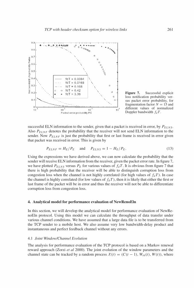
Figure 7. Successful explicitloss notification probability ver-sus packet error probability, forfragmentation factor N = 15 anddifferent values of normalizedDoppler bandwidth fdT .
successful ELN information to the sender, given that a packet is received in error, by PELNS .Also PELNF denotes the probability that the receiver will not send ELN information to thesender. Now PELNF is just the probability that first or last frame is received in error giventhat packet was received in error. This is given by
PELNF = HE/PE and PELNS = 1 − HE/PE. (13)
Using the expressions we have derived above, we can now calculate the probability that thesender will receive ELN information from the receiver, given the packet error rate. In figure 7,we have plotted PELNS versus PE for various values of fdT . It is obvious from figure 7 thatthere is high probability that the receiver will be able to distinguish corruption loss fromcongestion loss when the channel is not highly correlated (for high values of fdT ). In casethe channel is highly correlated (for low values of fdT ), then it is likely that either the first orlast frame of the packet will be in error and thus the receiver will not be able to differentiatecorruption loss from congestion loss.
4. Analytical model for performance evaluation of NewRenoEln
In this section, we will develop the analytical model for performance evaluation of NewRe-noEln protocol. Using this model we can calculate the throughput of data transfer undervarious channel conditions. We have assumed that a large data file is to be transferred fromthe TCP sender to a mobile host. We also assume very low bandwidth-delay product andinstantaneous and perfect feedback channel without any errors.
4.1 Joint Window/Channel Evolution
The analysis for performance evaluation of the TCP protocol is based on a Markov renewalreward approach (Zorzi et al 2000). The joint evolution of the window parameters and thechannel state can be tracked by a random process X (t) = (C(t − 1), Wth(t), W(t)), where

262 Pawan Kumar Gupta and Joy Kuri
W(t) and Wth(t) are the window size and slow start threshold in slot t , respectively, andC(t − 1) is the channel state (bad, B, or good, G, corresponding to an erroneous or correcttransmission, respectively) in slot t − 1. This process is not a Markov process as its evolutionfrom a certain state not only depends on the parameters specified by X (t), but also on someother parameters like number of oustanding packets not yet acknowledged and the time atwhich these packets were transmitted. If we incorporate these parameters into the processdescription then the state space of the process would become very large and impractical toevaluate. To make the process Markov we will sample it at appropriate instants tk such thatX(k) := X (tk) is a Markov process.
Considering tk’s as the slots immediately following those in which either a timeout timerexpires or a loss recovery phase is successfully completed, we obtain a process X(k) =X (tk) which is Markov. At such instants, there are no outstanding packets and knowledgeof (C(t − 1), Wth(t), W(t)) is enough to characterize the window/channel evolution in thefuture. Also from the protocol rules, the value of W(tk) can only be equal to one (timeoutcase) or to Wth(t) (successful loss recovery). Note that the channel state at time tk − 1 can beeither bad or good in the timeout case, but can only be good for a successful loss recovery,which must be ended by successful transmission. Therefore, the state space of the processX(k) is given by
�X = {(C, Wth, 1), C = B, G, 1 ≤ Wth ≤ �Wmax/2�}∪ {(G, Wth, Wth), 1 ≤ Wth ≤ �Wmax/2�},
(14)
where the first set corresponds to timeout and the second set corresponds to successful recoveryphase. Note that the total number of states in this case is 3�Wmax/2� − 1.
For evaluating metrics of interest, such as throughput, we need to track transmissionattempts, successful transmissions and time between successive sampling instants. In orderto be able to characterize these quantities, we consider a semi-Markov process which admitsX(k) as its embedded Markov chain. That is, we label transitions of the chain X(k) withtransition metrics, which track the (possibly random) events which determine time delay,transmissions, and successes. For a given transition, let Nd be the associated number of slots,Nt the number of transmissions, and Ns the number of successful transmissions.
4.2 Semi-Markov Analysis
Let tk be the kth sampling instant determined according to the above rules (without loss ofgenerality, assume t1 = 1). We define cycle k as the time evolution of the system betweenthe two consecutive sampling instants tk and tk+1. The statistical behavior of a cycle onlydepends on the channel state at time tk − 1 and on the slow start threshold and window size attime tk . Also, we assume that the process is stationary, so that everything is independent of k.When we look at the evolution of the process during a generic cycle k, it is implicit in whatfollows that system variables are conditioned on the pair of states X(k), X(k + 1) ∈ �X,where X(k) = (C(tk − 1), Wth(tk), W(tk)) and �X is the set of all possible values of X(k)
(state space of the sampled process). For simplicity of notation, let C(tk − 1) = C.Let the nth packet (where n ≥ 1) be the first packet of the cycle that was either erroneously
re-transmitted (for which no ELN is sent by the receiver) or erroneously transmitted forwhich receiver could not generate ELN. Thus in this part of the cycle there will be n − 1successes and these will only affect the window size evolution. The failures that get recoveredby successful retransmission based on ELN will be counted as single successes and affect
TCP with header checksum option for wireless links 263
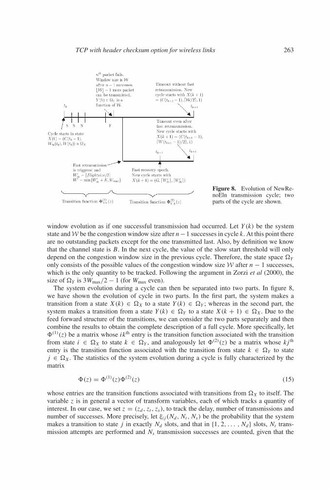
Figure 8. Evolution of NewRe-noEln transmission cycle; twoparts of the cycle are shown.
window evolution as if one successful transmission had occurred. Let Y (k) be the systemstate and W be the congestion window size after n−1 successes in cycle k. At this point thereare no outstanding packets except for the one transmitted last. Also, by definition we knowthat the channel state is B. In the next cycle, the value of the slow start threshold will onlydepend on the congestion window size in the previous cycle. Therefore, the state space �Y
only consists of the possible values of the congestion window size W after n − 1 successes,which is the only quantity to be tracked. Following the argument in Zorzi et al (2000), thesize of �Y is 3Wmax/2 − 1 (for Wmax even).
The system evolution during a cycle can then be separated into two parts. In figure 8,we have shown the evolution of cycle in two parts. In the first part, the system makes atransition from a state X(k) ∈ �X to a state Y (k) ∈ �Y ; whereas in the second part, thesystem makes a transition from a state Y (k) ∈ �Y to a state X(k + 1) ∈ �X. Due to thefeed forward structure of the transitions, we can consider the two parts separately and thencombine the results to obtain the complete description of a full cycle. More specifically, let�(1)(z) be a matrix whose ikth entry is the transition function associated with the transitionfrom state i ∈ �X to state k ∈ �Y , and analogously let �(2)(z) be a matrix whose kj th
entry is the transition function associated with the transition from state k ∈ �Y to statej ∈ �X. The statistics of the system evolution during a cycle is fully characterized by thematrix
�(z) = �(1)(z)�(2)(z) (15)
whose entries are the transition functions associated with transitions from �X to itself. Thevariable z is in general a vector of transform variables, each of which tracks a quantity ofinterest. In our case, we set z = (zd, zt , zs), to track the delay, number of transmissions andnumber of successes. More precisely, let ξij (Nd, Nt , Ns) be the probability that the systemmakes a transition to state j in exactly Nd slots, and that in {1, 2, . . . , Nd} slots, Nt trans-mission attempts are performed and Ns transmission successes are counted, given that the

264 Pawan Kumar Gupta and Joy Kuri
system was in state i at time 0. Then, we have
�ij (zd, zt , zs) =∑
nd ,nt ,ns
ξij (nd, nt , ns)znd
d znt
t zns
s . (16)
In particular, the transition matrix of the embedded Markov chain is just given by
P = � (1, 1, 1) . (17)
The matrix of average delays can be found as
D = ∂� (zd, zt , zs)
∂zd
∣∣∣∣zd ,zt ,zs=1
= D1�(2)(1, 1, 1) + �(1)(1, 1, 1)D2, (18)
where,
D1 = ∂�(1) (zd, zt , zs)
∂zd
∣∣∣∣zd ,zt ,zs=1
D2 = ∂�(2) (zd, zt , zs)
∂zd
∣∣∣∣zd ,zt ,zs=1
(19)
The averages of other quantities like number of transmission attempts T and number ofsuccesses S can be similarly found. From the above quantities we can compute a number ofsteady-state performance parameters. In particular, we can evaluate the average throughput as
Throughput =
∑i∈�X
πi
∑j∈�X
Sij∑i∈�X
πi
∑j∈�X
Dij
, (20)
where πi , i ∈ �X, are the steady-state probabilities of the Markov chain with transitionmatrix P and can be computed using the expression π = πP. Note that, in order to computesteady-state performance from this analysis, knowledge of P = �(1, 1, 1) and of D, T and Sis sufficient. Detailed derivation for throughput is provided in Appendix I.
Now we will evaluate the transition functions �(1)(z) and �(2)(z). The major task hereis to correctly identify all possible transitions and the associated transition functions. Toderive these, we proceed as follows for each possible system state (transition origin): (i) a setof mutually exclusive events is identified, exhausting all possibilities; (ii) for each of thoseevents, based on the origin state and on the NewRenoEln protocol rules, the destination of thecorresponding transition is identified and the transition function is computed; (iii) transitionscorresponding to distinct events but leading to the same destination state are combined (i.e.,the corresponding transition functions are added), to obtain �(1)(z) and �(2)(z).
4.3 Computation of �(1)(z) for NewRenoEln
The first part of the cycle consists of either error-free transmissions or successful re-transmissions based on ELN information. Let X = X(k) = (C, Wth, W). The first part ofthe cycle has Ns = n − 1 successes. Conditioned on the value of n, the window size aftern − 1 successes is a deterministic function ω(n, W, Wth) of Wth and W that can be tabulatedand is assumed to be known. Therefore, the window size after n − 1 successes is denoted by
W = W(n) = ω(n, W, Wth). (21)
TCP with header checksum option for wireless links 265
We will define the transition function αC(n) based on the value of n and the channel state C
at the beginning of the first part of the cycle.
αC(n) ={
PCBPELNF z1dz
1t z
0s + PCBPELNSPBBz2
dz2t z
0s n = 1
(PCGz1dz
1t z
1s + PCBPELNSPBGz2
dz2t z
1s )αG(n − 1) n > 1.
(22)
The symbols used in the above equation are defined in previous section. Here n = 1 meansthat the first transmission attempt itself failed. The first term indicates the case where thereceiver failed to generate ELN information. The second term indicates the case where thesender received ELN information and attempted re-transmission in the subsequent slot. Thisre-transmission also failed due to bad channel condition. The number of successes in bothcases is 0 but the number of slots used and number of transmissions is 2 in the second caseas it includes the retransmission attempt also.
Let us consider n = 2 for the case when n > 1. In this case there is one success and thena failure. We use recursion to evaluate this case. We have already evaluated the expressionfor n = 1 and this is used again, as indicated here by the term αG(n − 1). The success canbe due to two cases. In the first case, the transmission was successful in the first attempt asthe channel was good. In this case the number of successes, number of transmission attemptsand number of slots all are one. If the first transmission attempt is unsuccessful then withprobability PELNS , the sender will receive ELN information and will attempt re-transmission.This re-transmission will be successful if the channel is good in the next slot. In this case thenumber of successes is still one, but the number of transmission attempts and number of slotsis two. The same explanation can be easily extended to the cases for n > 2 also. With this wecan now write the expression for �(1)(z) as
�1XY (zd, zt , zs) =
∑n∈C(X,Y )
αC(n)
where C(X, Y ) = {n : ω(n, W, Wth) = W}(23)
4.4 Computation of �(2)(z) for NewRenoEln
The second part of the cycle can also be fully characterized by appropriately labelling tran-sitions and counting events. Let ε(Y ) be an exhaustive set of mutually exclusive events asso-ciated with transitions from state Y (k) = Y . Also, let dY (.) : ε(Y ) → �X be a well definedfunction, giving the destination state corresponding to each event in ε(Y ). Note that thisrequires that events be defined so that the destination is uniquely specified. However, dis-tinct events may lead to the same destination. Also, let the function � map each event to thecorresponding transition function. We can then formally find the YXth entry of the transitionfunction matrix �(2)(z) as
�2YX(z) =
∑A∈D(X,Y )
ψ(A), (24)
where D(X, Y ) = {A ∈ ε(Y ) : dY (A) = X} is the set of all events leading from Y ∈ �Y
to X ∈ �X during phase two. We evaluate all such events for the second phase of the cyclebelow.
For simplicity of notation, in what follows we denote by 0 the slot where the first phaseends, so that the first slot in the second phase corresponds to time 1. Define ϕij (k, x, y) as

266 Pawan Kumar Gupta and Joy Kuri
the probability that there are k successes in slots 1 through y, when the sender has exactly x
packets to send and it transmits all of them, and the channel is in state j at y, given that thechannel was in state i at time 0. Recursive solution for this is as follows:
ϕij (k, x, y) =
⎧⎪⎪⎪⎪⎪⎪⎪⎪⎪⎪⎪⎪⎪⎪⎪⎪⎨⎪⎪⎪⎪⎪⎪⎪⎪⎪⎪⎪⎪⎪⎪⎪⎪⎩
0, for k, x, y < 0
0, for k > x, k > y, x > y
0, for (k = x = y = 0 and i = j)
1, for (k = x = y = 0 and i = j)
PiGϕGj (k − 1, x − 1, y − 1)
+PiBPELNSPBGϕGj (k − 1, x − 1, y − 2)
+PiBPELNF ϕBj (k, x − 1, y − 1)
+PiBPELNSPBBϕBj (k, x − 1, y − 2), otherwise.
(25)
The first term in the recursive expression given above indicates that the first transmissionattempt is successful. The second term indicates that the first transmission attempt was unsuc-cessful but the sender received ELN information and the re-transmission was successful. Thethird term indicates that the first transmission attempt was unsuccessful and the sender didnot get any ELN information. The fourth term indicates that the first transmission attemptwas unsuccessful, the sender received ELN information but the re-transmission was unsuc-cessful.
We will consider two cases: one in which fast re-transmission is not triggered and the otherin which fast re-transmission is triggered.
4.4a Fast re-transmission is not triggered: In the second part of the cycle the congestionwindow is denoted by W and the sender can now send {1, 2, . . . , �W� − 1} more packets.Let Nps < K denote the number of packets that are successfully transmitted. In this casethe timeout timer will expire and the lost packet will be re-transmitted in slot tk+1 = T0
(Timeout). We assume in following sections that the timeout value is always very large ascompared to the congestion window size and the sender will exhaust its window of packetsbefore the timeout timer expires. Note that the value of the window size at timeout will stillbe equal to W (recall that duplicate ACKs before fast re-transmission do not advance thewindow), so that after timeout the algorithm will set Wth = �W/2�, W = 1. This event willtherefore, lead to state X(k + 1) = (C, �W/2�, 1) with transition function
z(T0−1)d
2(�W�−1)∑y=�W�−1
K−1∑Nps=0
ϕBB(Nps, �W� − 1, y)PBC(T0 − y − 1)zNs(B,Nps)s z
yt
+ z(T0−1)d
2(�W�−1)∑y=�W�−1
K−1∑Nps=1
ϕBG(Nps, �W� − 1, y)PGC(T0 − y − 1)zNs(G,Nps)s z
yt
(26)
where 0 ≤ Ns(B, Nps),Ns(G, Nps) ≤ Nps . The expression here is calculated forNps ≤ K−1successes when the sender has �W� − 1 packets to transmit and it uses y slots to transmitthem. Clearly y can range from �W� − 1 to 2(�W� − 1) as each packet transmission willutilize a minimum of one and a maximum of two slots, irrespective of its success or failure.
TCP with header checksum option for wireless links 267
The two terms account for the two possibilities for the channel state after �W� − 1 packetsare transmitted. Ns(B, Nps) and Ns(G, Nps) are random variables and their exact valueswill depend on further evolution of the chain. This is because we may or may not countcertain packets as successes, depending on their possible retransmission in the next cycle.We will only consider bounds for these variables for the best and worst cases as shownabove.
4.4b Fast re-transmission is triggered: In this case, the sender receives the K th dupli-cate ACK and fast re-transmit is triggered right after the K th successful transmission in{1, 2, . . . , �W�−1}. Clearly in this case, �W� > K . There are many sub-cases possible hereand we will consider them one by one.
Single loss before the K th duplicate ACK and re-transmission successful: In this case asingle loss occurs in the cycle and it is the loss that resulted in the state transition from stateX to state Y . Since there is no other loss, the sender will receive the K th duplicate ACKafter K packet transmissions. Upon receiving the K th duplicate ACK, the slow start thresholdwill be updated to W ′
th = �f lightsize/2� and the congestion window size will be updatedto W ′ = min {W ′
th + K, Wmax}. In this particular case, the flightsize is K + 1. The lostpacket that resulted in the K duplicate ACKs will now be re-transmitted in the next slot. Weconsider that re-transmission is successful and loss recovery phase is completed and a newcycle starts with the state X(k + 1) = (G, �W ′
th�, �W ′th�) and the transition function is given
by
zK+1s
2(K+1)∑y=K+1
ϕBG(K + 1, K + 1, y)zy
dzyt . (27)
Single loss before the K th duplicate ACK and re-transmission failure: In this case weconsider that the retransmitted packet also fails. The sender can continue to transmit morepackets if allowed by the congestion window and flightsize. In this particular case the sendercan send more packets only if W ′ > K + 1. We will consider these two cases separately.
W′ ≤ K + 1 :
Here the sender will stall after re-transmission and wait for timeout and the new cycle willstart after timeout with the state X(k + 1) = (C, �W ′/2�, 1) and the transition function isgiven by
zKs
2K∑y=K
ϕBG(K, K, y)
[PGBPELNF PBC(T0 − 1)z
y+1t z
(T0+y)
d
+PGBPELNSPBBPBC(T0 − 1)zy+2t z
(T0+y+1)
d
](28)
W′ > K + 1 :
In this case the sender can send W ′ − (K + 1) more packets and some of these packetsmay be successfully received by the receiver, thereby generating more duplicate ACKs. Eachof these duplicate ACKs will increment the congestion window by one, thereby allowing onemore packet transmission. This will continue until the number of packets in flight equals thecongestion window or the congestion window reaches Wmax. We will assume that the sender
268 Pawan Kumar Gupta and Joy Kuri
stalls when the congestion window size is M; then the next cycle starts after timeout withstate X(k + 1) = (C, �M/2�, 1), M = W ′, W ′ + 1, . . . , Wmax. Let us denote by Npt thenumber of packets transmitted after the failure of re-transmission and before the sender stalls,waiting for a timeout. Then Npt = M − (K + 1). Also let w denote the number of slotsused to transmit these Npt packets. Then the transition function when M < Wmax is givenby
2K∑y=K
ϕBG(K, K, y)
⎡⎢⎢⎢⎢⎢⎢⎢⎢⎢⎢⎢⎢⎢⎢⎣
PGBPELNF
2Npt∑w=Npt
⎧⎪⎪⎪⎨⎪⎪⎪⎩
ϕBB(M − W ′, Npt , w)
×PBC (T0 − 1 − w)
×zy+1+wt zNs+K
s z(T0+y)
d
⎫⎪⎪⎪⎬⎪⎪⎪⎭
+PGBPELNSPBB
2Npt∑w=Npt
⎧⎪⎪⎪⎨⎪⎪⎪⎩
ϕBB(M − W ′, Npt , w)
×PBC (T0 − 1 − w)
×zNs+Ks z
y+2+wt z
(T0+y+1)
d
⎫⎪⎪⎪⎬⎪⎪⎪⎭
⎤⎥⎥⎥⎥⎥⎥⎥⎥⎥⎥⎥⎥⎥⎥⎦
(29)
Note that the total number of successful transmissions to be counted in this case is Ns + K
where K is a constant and Ns is a random variable with range 0 ≤ Ns ≤ M − W ′.The case where M = Wmax is more complicated. Here the number of successful packet
transmissions on the channel after the re-transmission fails could range from M −W ′ to Npt .We will approximate the expression in this case taking the maximum value. This approx-imation hardly introduces any error in the analytical results shown later. We can write thetransition function in this case as
2K∑y=K
ϕBG(K, K, y)
⎡⎢⎢⎢⎢⎢⎢⎢⎢⎢⎢⎢⎢⎢⎢⎣
PGBPELNF
2Npt∑w=Npt
⎧⎪⎪⎪⎨⎪⎪⎪⎩
ϕBG(Npt , Npt , w)
×PGC (T0 − 1 − w)
×zy+1+wt zNs+K
s z(T0+y)
d
⎫⎪⎪⎪⎬⎪⎪⎪⎭
+PGBPELNSPBB
2Npt∑w=Npt
⎧⎪⎪⎪⎨⎪⎪⎪⎩
ϕBG(Npt , Npt , w)
×PGC (T0 − 1 − w)
×zy+2+wt zNs+K
s z(T0+y+1)
d
⎫⎪⎪⎪⎬⎪⎪⎪⎭
⎤⎥⎥⎥⎥⎥⎥⎥⎥⎥⎥⎥⎥⎥⎥⎦
. (30)
In this case too Ns is a random variable with range 0 ≤ Ns ≤ Npt .
Multiple losses before the K th duplicate ACK and successful loss recovery: Before proceed-ing further we will define B(Nk, �1, y), K < Nk < �W�, 0 < �1 ≤ K, Nk ≤ y ≤ 2Nk , tobe the event that the K th success occurs at N th
k packet transmission and y th slot and the firstloss after the loss in slot 0 occurred at the �th
1 packet transmission. (Note that since Nk > K ,there must be a packet loss before the K th success). The probability of this event is given as

TCP with header checksum option for wireless links 269
follows:
P [B (Nk, �1, y)] =
⎧⎪⎪⎪⎪⎪⎪⎪⎪⎪⎪⎪⎪⎨⎪⎪⎪⎪⎪⎪⎪⎪⎪⎪⎪⎪⎩
PBBPELNF ϕBG (K, Nk − 1, y − 1)
+PBBPELNSPBBϕBG (K, Nk − 1, y − 2) ,
for �1 = 1; Nk = K + 1, ..., �W� − 1
2�1∑w=�1
{ϕBB (�1 − 1, �1, w)
×ϕBG(K − �1 + 1, Nk − �1, y − w)}for �1 = 2, . . . , K; Nk = K + 1, . . . , �W� − 1.
(31)
We are considering the case where multiple losses occur but the sender is able to recover fromthe losses successfully without waiting for timeout. Upon receiving the K th duplicate ACKthe slow start threshold will be updated to W ′
th = �f lightsize/2� and the window size willbe updated to W ′ = min{W ′
th +K, Wmax}. In this particular case the flightsize is Nk +1. Nowthe sender will re-transmit the lost packet. Here we consider that this retransmission succeedsand also the next Nk − K packets are successfully re-transmitted (note that the N th
k packettransmission resulted in the K th duplicate ACK and thus a total of Nk −K more packets needto be transmitted for loss recovery to be complete) and thus loss recovery is complete. In thiscase the next cycle starts in the state X(k + 1) = (G, �(Nk + 1)/2�, �(Nk + 1)/2�) and thetransition function is given by
2Nk∑y=Nk
K∑�1=1
2(Nk+1−K)∑w=Nk+1−K
[P [B (Nk, �1, y)] ϕGG (Nk + 1 − K, Nk + 1 − K, w)
×zy+w+1d z
y+w+1t zNk+1
s
]
(32)
Multiple losses before the K th duplicate ACK and unsuccessful loss recovery: Many sub-cases are possible here depending on the number of successful re-transmissions after the K th
duplicate ACK is received. The analysis becomes very complicated if we track each loss andeach retransmission attempt. Instead, some approximations can be made without affectingthe overall analysis depending on the desired accuracy of the results. Here we have shownthe transition function for one case where first re-transmission fails. The sender will stallafter re-transmitting the original lost packet and wait for timeout and the new cycle will startafter timeout with the state X(k + 1) = (C, �W ′/2�, 1) and the transition function is givenby
zNs
s
2Nk∑y=Nk
K∑�1=1
P [B (Nk, �1, y)]
[PGBPELNF PBC (T0 − 1) z
y+1t z
(T0+y)
d
+PGBPELNSPBBPBC (T0 − 1) zy+2t z
(T0+y+1)
d
]
(33)
where �1 − 1 ≤ Ns ≤ K .Similarly, other sub-cases can be evaluated. Using these expressions we can evaluate the
throughput of data transfer when the NewRenoEln protocol is used.
270 Pawan Kumar Gupta and Joy Kuri
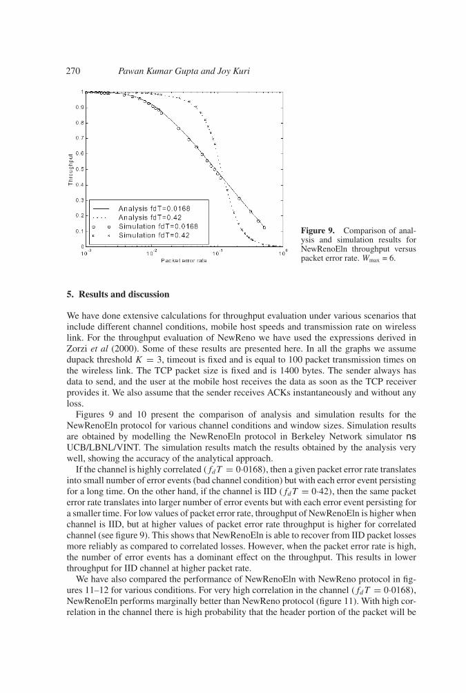
Figure 9. Comparison of anal-ysis and simulation results forNewRenoEln throughput versuspacket error rate. Wmax = 6.
5. Results and discussion
We have done extensive calculations for throughput evaluation under various scenarios thatinclude different channel conditions, mobile host speeds and transmission rate on wirelesslink. For the throughput evaluation of NewReno we have used the expressions derived inZorzi et al (2000). Some of these results are presented here. In all the graphs we assumedupack threshold K = 3, timeout is fixed and is equal to 100 packet transmission times onthe wireless link. The TCP packet size is fixed and is 1400 bytes. The sender always hasdata to send, and the user at the mobile host receives the data as soon as the TCP receiverprovides it. We also assume that the sender receives ACKs instantaneously and without anyloss.
Figures 9 and 10 present the comparison of analysis and simulation results for theNewRenoEln protocol for various channel conditions and window sizes. Simulation resultsare obtained by modelling the NewRenoEln protocol in Berkeley Network simulator nsUCB/LBNL/VINT. The simulation results match the results obtained by the analysis verywell, showing the accuracy of the analytical approach.
If the channel is highly correlated (fdT = 0·0168), then a given packet error rate translatesinto small number of error events (bad channel condition) but with each error event persistingfor a long time. On the other hand, if the channel is IID (fdT = 0·42), then the same packeterror rate translates into larger number of error events but with each error event persisting fora smaller time. For low values of packet error rate, throughput of NewRenoEln is higher whenchannel is IID, but at higher values of packet error rate throughput is higher for correlatedchannel (see figure 9). This shows that NewRenoEln is able to recover from IID packet lossesmore reliably as compared to correlated losses. However, when the packet error rate is high,the number of error events has a dominant effect on the throughput. This results in lowerthroughput for IID channel at higher packet rate.
We have also compared the performance of NewRenoEln with NewReno protocol in fig-ures 11–12 for various conditions. For very high correlation in the channel (fdT = 0·0168),NewRenoEln performs marginally better than NewReno protocol (figure 11). With high cor-relation in the channel there is high probability that the header portion of the packet will be
TCP with header checksum option for wireless links 271
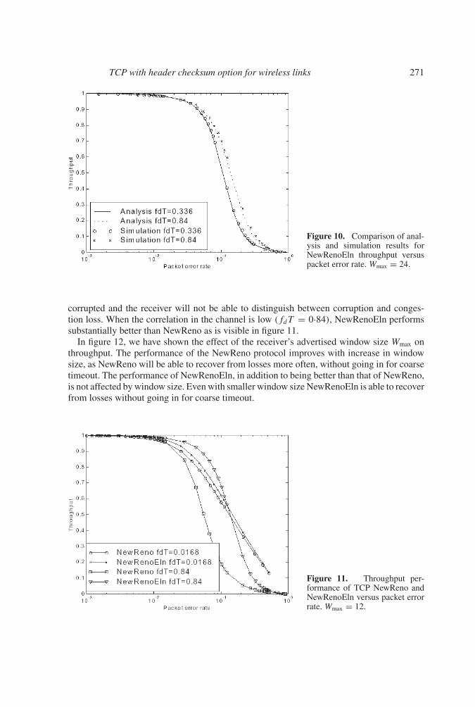
Figure 10. Comparison of anal-ysis and simulation results forNewRenoEln throughput versuspacket error rate. Wmax = 24.
corrupted and the receiver will not be able to distinguish between corruption and conges-tion loss. When the correlation in the channel is low (fdT = 0·84), NewRenoEln performssubstantially better than NewReno as is visible in figure 11.
In figure 12, we have shown the effect of the receiver’s advertised window size Wmax onthroughput. The performance of the NewReno protocol improves with increase in windowsize, as NewReno will be able to recover from losses more often, without going in for coarsetimeout. The performance of NewRenoEln, in addition to being better than that of NewReno,is not affected by window size. Even with smaller window size NewRenoEln is able to recoverfrom losses without going in for coarse timeout.
Figure 11. Throughput per-formance of TCP NewReno andNewRenoEln versus packet errorrate. Wmax = 12.
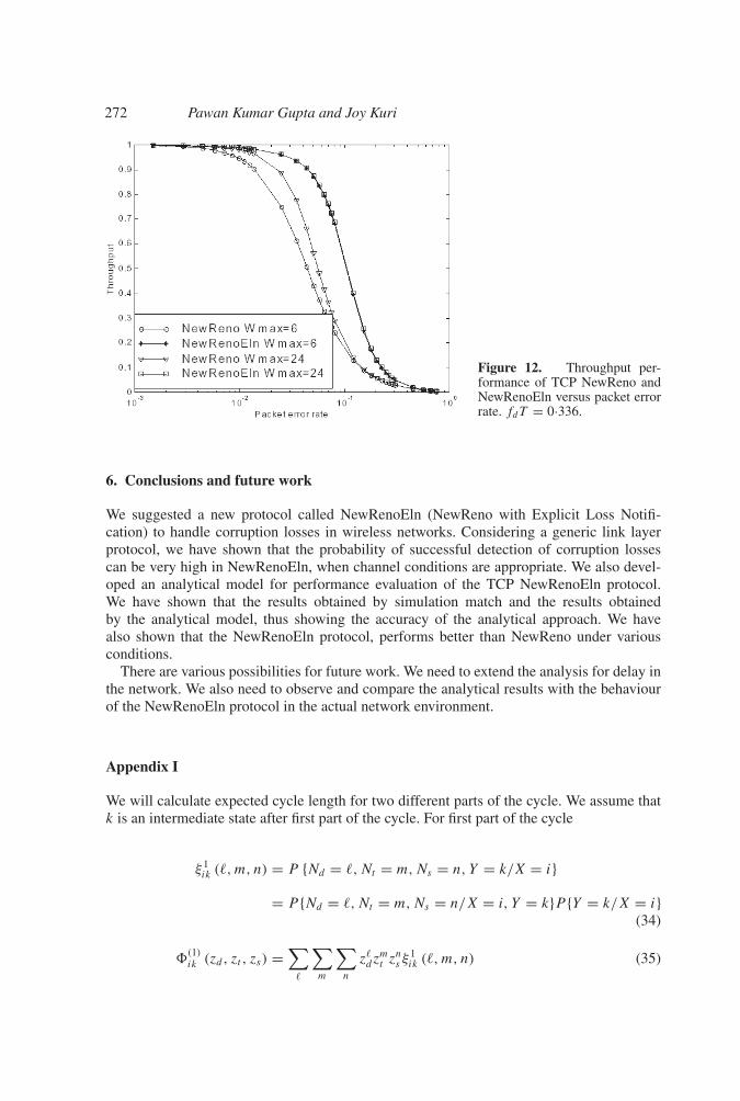
272 Pawan Kumar Gupta and Joy Kuri
Figure 12. Throughput per-formance of TCP NewReno andNewRenoEln versus packet errorrate. fdT = 0·336.
6. Conclusions and future work
We suggested a new protocol called NewRenoEln (NewReno with Explicit Loss Notifi-cation) to handle corruption losses in wireless networks. Considering a generic link layerprotocol, we have shown that the probability of successful detection of corruption lossescan be very high in NewRenoEln, when channel conditions are appropriate. We also devel-oped an analytical model for performance evaluation of the TCP NewRenoEln protocol.We have shown that the results obtained by simulation match and the results obtainedby the analytical model, thus showing the accuracy of the analytical approach. We havealso shown that the NewRenoEln protocol, performs better than NewReno under variousconditions.
There are various possibilities for future work. We need to extend the analysis for delay inthe network. We also need to observe and compare the analytical results with the behaviourof the NewRenoEln protocol in the actual network environment.
Appendix I
We will calculate expected cycle length for two different parts of the cycle. We assume thatk is an intermediate state after first part of the cycle. For first part of the cycle
ξ 1ik (�, m, n) = P {Nd = �, Nt = m, Ns = n, Y = k/X = i}
= P {Nd = �, Nt = m, Ns = n/X = i, Y = k}P {Y = k/X = i}(34)
�(1)ik (zd, zt , zs) =
∑�
∑m
∑n
z�dz
mt zn
s ξ1ik (�, m, n) (35)
TCP with header checksum option for wireless links 273
and for second part of the cycle
ξ 2kj (�, m, n) = P {Nd = �, Nt = m, Ns = n, Xf = j/Y = k}
= P {Nd = �, Nt = m, Ns = n/Y = k, Xf = j}P {Xf = j/Y = k}(36)
Xf is the starting state belonging to �X in the next cycle.
�(2)kj (zd, zt , zs) =
∑�
∑m
∑n
z�dz
mt zn
s ξ2kj (�, m, n) (37)
Considering a single element from the matrix of average delays
D1 [i, k] := ∂�(1)ik (zd, zt , zs)
∂zd
∣∣∣∣∣zd ,zt ,zs=1
=∑
�
∑m
∑n
�.ξ 1ik (�, m, n)
=∑
�
∑m
∑n
�P {Nd = �, Nt = m, Ns = n, /X = i, Y = k}P {Y = k/X = i}
=∑
�
�P {Nd = �/X = i, Y = k} P {Y = k/X = i}
= E {Delay in reaching state k ∈ �Y /X = i, Y = k} P {Y = k/X = i}= E
{T (1)/X = i, Y = k
}P {Y = k/X = i}
(38)
Similarly,
D2 [k, j ] := ∂�(2)kj (zd, zt , zs)
∂zd
∣∣∣∣∣zd ,zt ,zs=1
=∑
�
∑m
∑n
�.ξ 2kj (�, m, n)
= E{T (2)/Y = k, Xf = j
}P
{Xf = j/Y = k
} (39)
T (1), T (2) are the cycle lengths for the first and second part of the cycle respectively. Expecteddelay for the complete cycle for the given initial and final state is obtained as follows. Fromthe definitions of D1, φ(2), D2 and φ(1), we have
(D1φ(2) (1, 1, 1)) [i, j ]
=∑
k
E{T (1)/X = i, Y = k}P {Y = k/X = i} P {Xf = j/Y = k}
=∑
k
E{T (1)/X = i, Y = k}P {Y = k/X = i} P {Xf = j/Y = k, X = i}
=∑
k
E{T (1)/X = i, Y = k}P {Xf = j, Y = k/X = i}(40)
274 Pawan Kumar Gupta and Joy Kuri
The second step is valid in the equation above as the process is Markov and P {Xf =j/Y = k} does not change with inclusion of X = i in the expression. The probability of thenext state Xf being j is completely independent of initial state X = i, if the intermediatestate Y = k is specified.∑
j
(D1φ(2) (1, 1, 1)) [i, j ]
=∑
j
∑k
E{T (1)/X = i, Y = k}P {Xf = j, Y = k/X = i}
=∑
k
∑j
E{T (1)/X = i, Y = k}P {Xf = j, Y = k/X = i}
=∑
k
E{T (1)/X = i, Y = k}P {Y = k/X = i}
(41)
The interchange of order of summation in the above equation is valid as the summation isdone over finite state space.∑
i
πi
∑j
(D1φ(2) (1, 1, 1)) [i, j ]
=∑
i
P {X = i}∑
k
E{T (1)/X = i, Y = k}P {Y = k/X = i}
=∑
i
∑k
E{T (1)/X = i, Y = k}P {X = i, Y = k} = E{T (1)}
(42)
Similarly, ∑i
πi
∑j
(φ(1) (1, 1, 1) D2) [i, j ] = E{T (2)}. (43)
Thus, using equation (20), the expected cycle length is given by
∑i
πi
(∑j
D [i, j ]
)
=∑
i
πi
{∑j
(D1φ
(2) (1, 1, 1))
[i, j ] +∑
j
(φ(1) (1, 1, 1) D2
)[i, j ]
}
= E{T (1)} + E{T (2)} = E{T (1) + T (2)}.
(44)
In a similar manner, we can evaluate the expected number of successes and write theexpression for throughput as
Throughput = Expected number of successes
Expected cycle length=
∑i∈�X
πi
∑j∈�X
Sij∑i∈�X
πi
∑j∈�X
Dij
(45)
TCP with header checksum option for wireless links 275
The authors would like to thank Mr Satish Kulkarni and many others from C-DOT and CEDTfor their support in this work.
References
Bakshi B S, Krishna P, Vaidya N H, Pradhan D K 1997 Improving performance of TCP over wirelessnetworks. In Proc. 17th Int. Conf. Distributed Computing Systems
Balakrishnan H, Padmanabhan V N, Seshan S, Katz R H 1997 A comparison of mechanisms forimproving TCP performance over wireless links. ACM/IEEE Trans. Networking 56: pp 756–759
Balakrishnan H, Katz R H 1998 Explicit Loss Notification and Wireless Web Performance. In Proc.IEEE Globecom Internet Mini-Conference
Balan R K, Lee B P, Kumar K R R, Jacob L, Seah W K G, Ananda A L 2001 TCP HACK: TCP headerchecksum option to improve performance over lossy links. In Proc. IEEE INFOCOMM
Caceres R, Iftode L 1995 Improving the performance of reliable transport protocols in mobile com-puting environments. IEEE J. Select. Areas Commun. 13: pp 850–857
Chen W, Lee J 2000 Some mechanisms to improve TCP/IP performance over wireless and mobilecomputing environment. In Proc. 7th Int. Conf. Parallel and Distributed Systems
Floyd S, Henderson T The NewReno Modification to TCP’s Fast Recovery Algorithm, RFC2582Goff T, Moronski J, Phatak D S, Gupta V 2000 Freeze TCP a true end to end TCP enhancement
mechanism for mobile environments. In Proc. IEEE INFOCOMMGupta Pawan Kumar, Joy Kuri 2002 Reliable ELN to enhance throughput of TCP over wireless links
via TCP header checksum. In Proc. IEEE GLOBECOMKumar A 1998 Comparative performance analysis of versions of TCP in a local network with a lossy
link. ACM/IEEE Trans. Networking pp 485–498 1998Parsa C, Aceves J J G L 2000 Differentiating congestion vs random loss: A method for improving
TCP performance over wireless links. In Proc. IEEE WCNCPeng F, Ma J A proposal to apply ECN into Wireless and Mobile Networks, draft-fpeng-ecn-03.txtPostel J Transmission Control Protocol. RFC793Sinha P, Venkitaraman N, Sivakumar R, Bharghavan V 1999 WTCP: A Reliable Transport Protocol
for Wireless Wide-Area Networks. In Proc. ACM MOBICOMM’99Stevens W R 1994 TCP/IP Illustrated. 1: Reading, MA: Addison WesleyUCB/LBNL/VINT Network Simulator - ns (version 2). URL: http://www.isi.edu/nsnam/nsVaidya N 1997 Discriminating congestion losses from wireless losses using inter arrival times at the
receiver. In Proc. IEEE ASSETZorzi M, Rao R R, Milstein L B 1995 On the accuracy of a first-order Markov model for data
transmission on fading channels. In Proc. IEEE ICUPC’95 pp 211–215Zorzi M, Chockalingam A, Rao R R 2000 Throughput analysis of TCP on channels with memory.
IEEE J. Select. Areas Commun. 18: pp 1289–1300