TCP – Random Early Detection (RED) mechanism for ...

Rochester Institute of Technology Rochester Institute of Technology

RIT Scholar Works RIT Scholar Works

Theses

7-2-2015

TCP – Random Early Detection (RED) mechanism for Congestion TCP – Random Early Detection (RED) mechanism for Congestion

Control Control

Asli Sungur [email protected]

Follow this and additional works at: https://scholarworks.rit.edu/theses

Recommended Citation Recommended Citation Sungur, Asli, "TCP – Random Early Detection (RED) mechanism for Congestion Control" (2015). Thesis. Rochester Institute of Technology. Accessed from

This Thesis is brought to you for free and open access by RIT Scholar Works. It has been accepted for inclusion in Theses by an authorized administrator of RIT Scholar Works. For more information, please contact [email protected].

https://scholarworks.rit.edu/

https://scholarworks.rit.edu/theses

https://scholarworks.rit.edu/theses?utm_source=scholarworks.rit.edu%2Ftheses%2F8904&utm_medium=PDF&utm_campaign=PDFCoverPages

https://scholarworks.rit.edu/theses/8904?utm_source=scholarworks.rit.edu%2Ftheses%2F8904&utm_medium=PDF&utm_campaign=PDFCoverPages

mailto:[email protected]

i

R.I.T

TCP – Random Early Detection (RED) mechanism for

Congestion Control

by

ASLI SUNGUR

This thesis is presented as part of the Degree of Master of Science in Network and

System Administration with emphasis in Networking

Committee Members:

Ali Raza

Muhieddin Amer

Nirmala Shenoy

Information Science and Technologies Department,

B. Thomas Golisano College of Computing & Information Sciences

Rochester Institute of Technology

Rochester, NY

July 2, 2015

ii

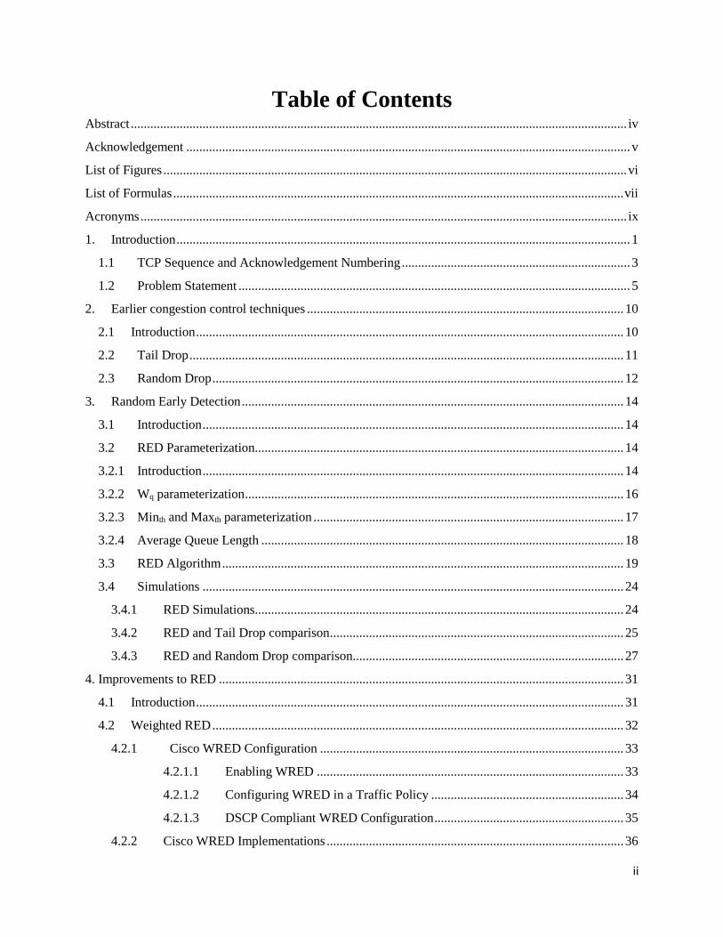
Table of Contents

Abstract ........................................................................................................................................................ iv

Acknowledgement ........................................................................................................................................ v

List of Figures .............................................................................................................................................. vi

List of Formulas .......................................................................................................................................... vii

Acronyms ..................................................................................................................................................... ix

1. Introduction ........................................................................................................................................... 1

1.1 TCP Sequence and Acknowledgement Numbering ...................................................................... 3

1.2 Problem Statement ........................................................................................................................ 5

2. Earlier congestion control techniques ................................................................................................. 10

2.1 Introduction ................................................................................................................................... 10

2.2 Tail Drop ..................................................................................................................................... 11

2.3 Random Drop .............................................................................................................................. 12

3. Random Early Detection ..................................................................................................................... 14

3.1 Introduction ................................................................................................................................. 14

3.2 RED Parameterization................................................................................................................. 14

3.2.1 Introduction ................................................................................................................................. 14

3.2.2 Wq parameterization .................................................................................................................... 16

3.2.3 Minth and Maxth parameterization ............................................................................................... 17

3.2.4 Average Queue Length ............................................................................................................... 18

3.3 RED Algorithm ........................................................................................................................... 19

3.4 Simulations ................................................................................................................................. 24

3.4.1 RED Simulations................................................................................................................. 24

3.4.2 RED and Tail Drop comparison .......................................................................................... 25

3.4.3 RED and Random Drop comparison................................................................................... 27

4. Improvements to RED ............................................................................................................................ 31

4.1 Introduction ................................................................................................................................... 31

4.2 Weighted RED .............................................................................................................................. 32

4.2.1 Cisco WRED Configuration ............................................................................................. 33

4.2.1.1 Enabling WRED .............................................................................................. 33

4.2.1.2 Configuring WRED in a Traffic Policy ........................................................... 34

4.2.1.3 DSCP Compliant WRED Configuration .......................................................... 35

4.2.2 Cisco WRED Implementations ........................................................................................... 36

iii

4.2.3 Juniper WRED Configuration ............................................................................................. 39

4.2.3.1 Enabling WRED .......................................................................................... 39

4.2.3.2 Configuring WRED in a Traffic Policy ....................................................... 40

4.2.4 Juniper WRED Implementations ........................................................................................ 43

4.3 Flow RED ...................................................................................................................................... 46

4.4 Adaptive RED ................................................................................................................................ 47

5. Conclusion .............................................................................................................................................. 50

6. Future work ............................................................................................................................................. 52

Glossary ...................................................................................................................................................... 53

References ................................................................................................................................................... 57

iv

Abstract

This thesis discusses the Random Early Detection (RED) algorithm, proposed by Sally

Floyd, used for congestion avoidance in computer networking, how existing algorithms compare

to this approach and the configuration and implementation of the Weighted Random Early

Detection (WRED) variation.

RED uses a probability approach in order to calculate the probability that a packet will be

dropped before periods of high congestion, relative to the minimum and maximum queue

threshold, average queue length, packet size and the number of packets since the last drop.

The motivation for this thesis has been the high QoS provided to current delay-sensitive

applications such as Voice-over-IP (VoIP) by the incorporation of congestion avoidance

algorithms derived from the original RED design [45]. The WRED variation of RED is not

directly invoked on the VoIP class because congestion avoidance mechanisms are not configured

for voice queues. WRED is instead used to prioritize other traffic classes in order to avoid

congestion to provide and guarantee high quality of service for voice traffic [43][44].

The most notable simulations performed for the RED algorithm in comparison to the Tail

Drop (TD) and Random Drop (RD) algorithms have been detailed in order to show that RED is

much more advantageous in terms of congestion control in a network. The WRED, Flow RED

(FRED) and Adaptive RED (ARED) variations of the RED algorithm have been detailed with

emphasis on WRED. Details of the concepts of forwarding classes, output queues, traffic

policies, traffic classes, class maps, schedulers, scheduler maps, and DSCP classification shows

that the WRED feature is easily configurable on tier-1 vendor routers.

v

Acknowledgement

I would like to express my gratitude to Dr. Ali Raza for his scholarly advice, valuable

time and encouragement. Dr. Ali Raza’s vast knowledge in networking has helped me achieve a

clear picture of concepts that were vital in my understanding of the complex algorithms detailed

in this paper. I thank him whole-heartedly.

Finally, I would like to thank my parents for their love and supporting me on my journey

towards the completion of my degree.

vi

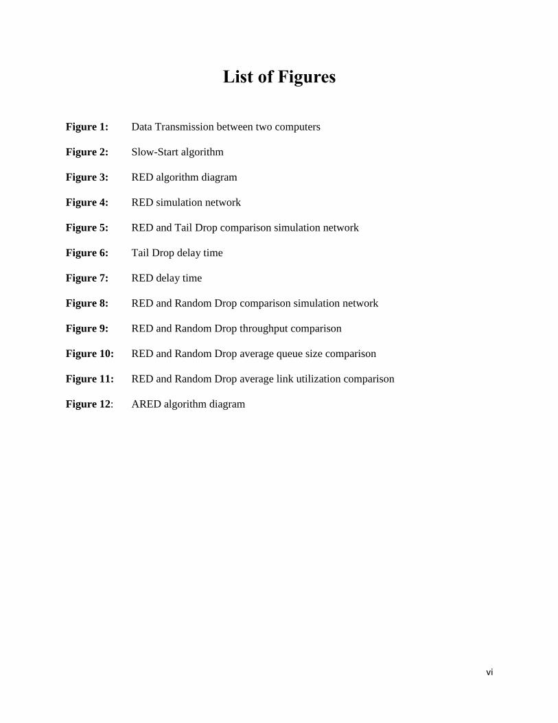
List of Figures

Figure 1: Data Transmission between two computers

Figure 2: Slow-Start algorithm

Figure 3: RED algorithm diagram

Figure 4: RED simulation network

Figure 5: RED and Tail Drop comparison simulation network

Figure 6: Tail Drop delay time

Figure 7: RED delay time

Figure 8: RED and Random Drop comparison simulation network

Figure 9: RED and Random Drop throughput comparison

Figure 10: RED and Random Drop average queue size comparison

Figure 11: RED and Random Drop average link utilization comparison

Figure 12: ARED algorithm diagram

vii

List of Formulas

Formula 1: Probability to drop a packet related to minimum and maximum queue threshold

Formula 2: Probability to drop a packet as more packets line up since last drop

Formula 3: Probability to drop a packet related to packet size

Formula 4: Average queue length

Formula 5: Dropped packets from connectioni

Formula 6: TCP Throughput formula

Formula 7: ARED algorithm weighted moving average

viii

List of Tables

Table 1: Cisco Traffic Classes with PHB and DSCP Values

Table 2: Juniper Forwarding Classes and Output Queues

Table 3: Juniper IP Precedence Classifier

Table 4: DSCP Code Points Mapping

ix

Acronyms

ACK Acknowledgement

AQM Active Queue Management

ARED Adaptive Random Early Detection

BA Behavior Aggregate

CBR Constant bitrate

DSCP Differentiated Services Code Point

ECN Explicit Congestion Notification

EWMA Exponential Weighted Moving Average

FIFO First In First Out

FRED Flow Random Early Detection

FTP File Transfer Protocol

HTTP Hypertext Transfer Protocol

IETF Internet Engineering Task Force

IOS Internetwork Operating System

IP Internet Protocol

ISN Initial Sequence Number

MSS Maximum Segment Size

NTWG Network Working Group

OSI Open Systems Interconnection

PHB Per Hop Behavior

PLP Packet Loss Priority

x

QM Queue Management

QoS Quality of Service

RED Random Early Detection

RTT Round Trip Time

SMTP Simple Mail Transfer Protocol

SYN Synchronize

TCP Transmission Control Protocol

TD Tail Drop

VoIP Voice over IP

WRED Weighted Random Early Detection

1

1. Introduction

Congestion occurs on a network when a device, such as a router, is receiving more packets

than it can handle. Because TCP responds to all data losses in a network, whether congestion or

non-congestion related, by invoking congestion control, the discarded packet caused by a bit

error would also be treated by TCP as if it were a congestion related packet loss [3][6][20]. There

are a number of internet applications within TCP such as the Hypertext Transfer Protocol

(HTTP), Simple Mail Transfer Protocol (SMTP), Secure Shell (SSH) and File Transfer Protocol

(FTP) such that congestion control becomes an increasingly difficult task as the users for these

applications grow. If packet losses occur mainly because of congestion in a linked network, then

TCP would perform well in such an environment. TCP does not perform so well in networks

where there is a high rate of packet losses that are caused by non-congestion related errors where

congestion control is unnecessarily invoked for these losses as per TCP behavior [6][20]. TCP

detects congestion only after a packet has already been dropped therefore a different mechanism

must be implemented or designed such that congestion is ‘avoided’ in order to improve network

performance [6][20].

“The problem with end to end congestion control schemes is that the presence of

congestion is detected through the effects of congestion, e.g., packet loss, increased round trip

time (RTT), changes in the throughput gradient, etc., rather than the congestion itself e.g.

overflowing queues.”[4]. Congestion control mechanisms, therefore, should be implemented at

the source; the gateways. “The gateway can reliably distinguish between propagation delay and

persistent queuing delay. Only the gateway has a unified view of the queuing behavior over time;

2

the perspective of individual connections is limited by the packet arrival patterns for those

connections. In addition, a gateway is shared by many active connections with a wide range of

roundtrip times, tolerances of delay, throughput requirements, etc.; decisions about the duration

and magnitude of transient congestion to be allowed at the gateway are best made by the gateway

itself.” [1, p.1].

A new mechanism called Random Early Detection (RED) was proposed by Sally Floyd

[1]. RED is an Active Queue Management (AQM) mechanism that is implemented at the

gateway in order to ‘avoid’ congestion rather than ‘respond’ to a situation that may not even be

congestion related. RED addresses issues caused by the TD and RD schemes, detailed later in

this paper, by detecting and avoiding congestion earlier on. Avoiding global synchronization and

being unbiased against bursty traffic are two areas that RED has shown to be advantageous in

comparison to older and existing congestion control mechanisms [4]. Global synchronization is

the pattern of all TCP/IP connections simultaneously starting and stopping their transmission of

data during periods of congestion. Once a packet is lost and congestion is detected and all

connections simultaneously reduce their transmission rate and restart transmission at the same

time, this will lead to a continuous cycle of congestion therefore an inefficient use of bandwidth

[1]. Algorithms such as TD penalize flows that transmit bursts of data in one go by dropping

packets from these flows that may consume even a small amount of bandwidth, therefore an

unfair algorithm. RED is unbiased against such bursty flows, allowing as much data to be

successfully sent before slowing down transmission from flows randomly to avoid congestion

[1][4]. To fully understand the algorithms detailed in this paper, it is crucial to first understand

how TCP data packet sequence and acknowledgement numbering works.

3

1.1 TCP Sequence and Acknowledgement Numbering

Each data packet that is transmitted is assigned a sequence number in order to keep track

of successful data transmission with the cooperation of acknowledgements (ACKs) received

from the receiver. For every data segment transmitted, an ACK is sent back to the sender to

confirm the successful transmission of the data therefore ACKs are used for flow control, error

control and congestion control. The sender and receiver both keep track of each other’s sequence

and acknowledgement numbers to ensure that packets arrive successfully and in the correct

order. An ACK can also ‘piggyback’ on or append to a data segment being sent in the opposite

direction. The Sequence Number in the TCP Header is 4 bytes (32 bits) long and is assigned to

every transmitted data packet. The 32 bit Acknowledgement Number is sent in the opposite

direction to confirm receipt of the data received by the sender. The Window Size indicates the

number of bytes that the receiver is currently willing to receive. Depending on the algorithm

used, the window size can increment such that the sender can send more data at one time as long

as the receiver has the capacity to receive that amount of data. Sequence and acknowledgement

numbers are incremented in terms of bytes and not segments. To grasp how TCP congestion

control works, it is important to first understand how sequence numbers are assigned and the

expected acknowledgement numbers in return. Figure 1 displays an example of data

transmission along with sequence and acknowledgement numbering:

4

A B

Seq = 1, Ack = 1

A B

Send 200 bytes of data

Seq = 0, Ack = 101

A B


Seq = 101, Ack = 201


The ACK for B piggybacks on the data sent in the opposite direction. B sends A 200 bytes of data. B also now acknowledges the 100 bytes of data received from A by

sending an ACK of 101 (100 + 1 Ack = 101).

A sends B 100 bytes of data. The next time A sends data to B, it must add 100 bytes to update its current Sequence Number of 1

(100 + 1 Seq = 101) as shown in the 3rd transmission

A now updates its Sequence Number to 101 as per the 1st tranmission. A now ACKs the 200 bytes of data received from B (2nd tranmission) by sending back 201. A sends B 50 bytes of data.

A B

Seq = 201, Ack = 151

Data transmission is now complete and B sends a final ACK of 151 for the 50 bytes of data that it received in the 3rd transmission. B’s Sequence Number is

updated to 201 (200 + 1 Seq = 201)

No data sent, just ACK

Figure 1: Data Transmission between two computers showing Sequence and Acknowledgement

numbering. As shown, the connection between the two flows is full duplex meaning that data

transfer can be bidirectional (A B and B A)

The ideal situation in a network is where data transmitted always successfully reaches its

destination with the response of the expected ACK in return, but consistently maintaining this

ideal in a network is almost impossible. In reality, especially in larger scale networks, when data

packets are sent they may get lost along the way hence fail to reach their destination, bit errors

may and/or timeouts may occur and/or physical layer issues can completely stall transmission.

In either scenario it is important to understand how TCP flows detect a lost packet and how it can

5

differentiate between an out-of-order packet requiring retransmission with that of a packet that is

dropped because of congested queues. The focus in this paper is packet loss that occurs as a

result of network congestion such that the sender is transmitting more packets to the receiver

than the receiver’s advertised receiving capacity at that time. The slow-start sliding window

algorithm detailed in section 1.3 explains how packet loss is detected and when congestion

avoidance is invoked in order to ‘avoid’ congestion earlier.

1.2 Problem Statement

Congestion control in TCP works in a way such that the sender sends out data packet

segments to the receiver up to the window size1 advertised and if using the same LAN and

working with a small network, this scenario would not cause a considerable number of issues.

The problem starts to arise if there are intermediate slower links between the sender and receiver

in a bigger network where there is more flow of traffic of varying packet sizes [10]. The

intermediate router or link would also have to queue incoming packets to be sent out and if this

intermediate router no longer has buffer2 space to queue packets, more packets are dropped,

retransmission of packets are required causing a degradation in network performance. Hashem

states in [14] that early TCP had no actual congestion control policy and the only way the data

flow was controlled was by the receiver advertising a smaller window size but there was no

specification as to how congestion would be controlled. This can prove to be a big problem

especially in bigger networks where the only way traffic is controlled is by buffering packets

therefore all incoming packets thereafter would be discarded. At this point users at the end- 1 receiving capacity in terms of bytes (segment size) 2 area within the physical memory storage of a device, such as a router, where data is stored temporarily before it is

transferred to the next device

6

connections would have to wait indefinitely long periods of time before the buffers are no longer

full and hopefully before the gateway can slow down the responsible TCP connections. If the

flow of data is slow and the buffers remain full and all incoming packets are continually

discarded, there will be a stall in data transmission from all connections. Another issue that can

occur for the end-users is a network timeout. A timeout is one of the ways TCP detects

congestion and occurs when the sender does not receive an ACK within the calculated time of

the RTT and connections are forcefully closed. Forcefully closing connections means that the

sender would have to restart transmission of its data. The second way TCP detects congestion is

through three duplicate ACKs as explained in the slow-start algorithm.

The slow-start and congestion avoidance algorithms used by TCP were introduced in order to

control the amount of outstanding data [8]. The sender must first probe the network to determine

how much data it can inject it with and that is the purpose of the slow-start algorithm. The

variables used are cwnd, ACK, rwnd and ssthresh. Cwnd is the sender’s congestion window

limit as to how many segments it can send out while still receiving the correct number of ACKs

and ACK numbers. Rwnd is the receiver’s advertised window limit on the amount of data

segments the sender is allowed to send at that time. Ssthresh is the slow-start threshold that

determines whether to use slow-start or congestion avoidance once a packet loss is detected. The

retransmission timer is used by TCP to keep track of the ACKs received for segments

transmitted [11].

The slow start algorithm is a technique used at the start of a new connection or when

restarting segment transmission from a connection that has timed out. The sender first sends out

one Maximum Segment Size (MSS) which is the largest segment that the sender can transmit at

one time. For example, if the MSS is 1290 bytes and the cwnd is double that size (2580 bytes),

7

then the sender can send two segments at the start of the connection. Once the receiver

successfully receives these two packet segment, it sends out two ACKs back to the sender

informing it that it has successfully received the two window segments. The sender then sends

out four packets, and after receiving four ACKs for those four packets, sends out a window of

eight segments on the next trip. The sender’s window segment size increases exponentially per

RTT as long as the same number of ACKs are received to successfully acknowledge segments

that are sent [21][24][25]. In TCP Reno, congestion is observed by either of the two following

scenarios:

1) Timeout: As explained before, a timeout occurs when the sender does not receive an ACK

within the expected RTT. Once a timeout occurs, this indicates to the sender that a packet

has been lost and the sender goes into congestion avoidance mode. In the congestion

avoidance mode, the congestion window is reset to 1 which puts the sender back into slow-

start mode [41].

2) Duplicate ACKs: When a receiver receives a segment with a sequence number that it was

not expecting, then it responds to the sender by sending the same ACK it previously sent

with the expected sequence number; this is a duplicate of the ACK it sent before. At this

point the sender is not aware if the duplicate ACK received indicates that a segment was out

of order or lost and usually just two duplicate ACKs received means that the expected ACK

will soon be received and ordering will be sorted. If more than two duplicate ACKs are

received (minimum of three duplicate ACKs), then the sender is now sure that a segment has

been lost and performs a Fast Retransmit. In Fast Retransmit, the sender immediately

transmits the missing segment to the waiting receiver and half of the current send window

cwnd is saved as ssthresh. After Fast Retransmit, the sender enters the Fast Recovery phase

8

by maintaining the same larger window size but now slowing down transmission and

increasing the window size by one segment hence entering the congestion avoidance state.

Fast Recovery maintains higher throughput by not allowing the sender to go back into slow-

start mode and restarting transmission at one segment [41].

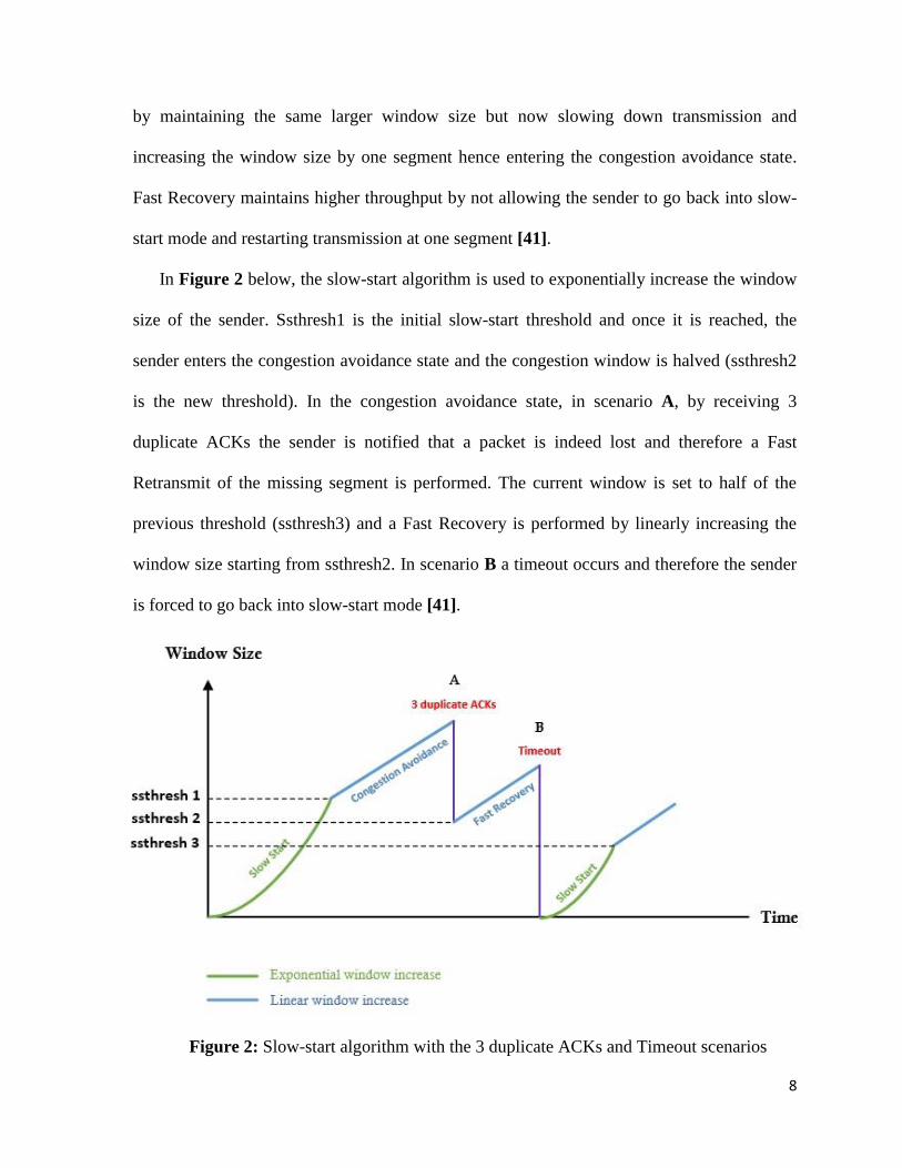
In Figure 2 below, the slow-start algorithm is used to exponentially increase the window

size of the sender. Ssthresh1 is the initial slow-start threshold and once it is reached, the

sender enters the congestion avoidance state and the congestion window is halved (ssthresh2

is the new threshold). In the congestion avoidance state, in scenario A, by receiving 3

duplicate ACKs the sender is notified that a packet is indeed lost and therefore a Fast

Retransmit of the missing segment is performed. The current window is set to half of the

previous threshold (ssthresh3) and a Fast Recovery is performed by linearly increasing the

window size starting from ssthresh2. In scenario B a timeout occurs and therefore the sender

is forced to go back into slow-start mode [41].

Figure 2: Slow-start algorithm with the 3 duplicate ACKs and Timeout scenarios

9

Once the congestion avoidance state is reached, the choice of which gateway congestion

control policy to use is dependent on the size of the network, services offered and the end-to-end

protocols supported. The slow-start phase of TCP requires short bursts of data to be sent but

RED can accommodate this short burst and therefore allows TCP’s connections to smoothly

open their windows while controlling the average queue size at the same time. RED is designed

to be used in conjunction with TCP’s existing congestion control techniques using timeouts and

duplicate ACKs. RED’s purpose is to more effectively notify the source of these timeouts and

duplicate ACKs by informing the gateway to drop packets earlier hence the source would be

notified to decrease its congestion window sooner [42]. Section 2 discusses the different

congestion avoidance mechanisms available in comparison to RED in order to improve network

throughput and delay.

10

2. Earlier congestion control techniques

2.1 Introduction

Queue Management mechanisms decide when to start dropping packets and at what gateway

source to drop these packets from. The main gateway based QM schemes implemented by TCP

are TD, RD, IP Source Quench and Congestion Indication (DECbit). The problem with these

schemes is that too many packets are dropped and the window size for connections decrease

abruptly hence slowing performance down greatly because of loss of throughput. If TCP

responds to all data losses by invoking congestion control, even if there is no actual congestion,

this can considerably slow down the performance of a network because of decreased window

sizes. With QM mechanisms such as TD and RD, congestion is detected once the buffer is

already full and incoming packets are dropped and therefore may not be the best choices in terms

of congestion avoidance but is rather suited for congestion recovery.

With Active Queue Management (AQM) congestion avoidance mechanisms, such as RED,

the dropping of packets occurs earlier on. The Internet Engineering Task Force (IETF)

recommended the use of AQM to provide congestion avoidance to tackle the common issue of

high packet loss rates in networks [17]. The Routers are enhanced to detect and notify

connections of impending congestion earlier, allowing them to slow down their transmission

rates before the router buffer overflows [18]; called proactive packet discard [34]. The goal of an

AQM mechanism is to achieve high link utilization, low queuing delay and improvement in

packet loss rates and fairness [18]. By keeping the average queue length small, AQM will

provide enough buffer space in the routers to absorb sudden bursts of traffic from connections

[16]. In [33], the queue law was proposed by Firoiu and Borden that states that “a router queue at

11

equilibrium has an average queue length as a function of the packet drop probability” and this

law is useful in configuring AQM mechanisms such as RED. RED is one of the most prominent

and widely studied congestion avoidance algorithms because of its early congestion notification

advantage over congestion control techniques such as Tail Drop and Random Drop.

2.2 Tail Drop

Because of the simplicity of FIFO queuing, the TD congestion control mechanism is widely

used on the Internet today. The two main issues with TD are the Full-queue problem and Lock-

out problem. With bursty traffic, TD queues fill up fast because TD does not provide an

indication of congestion to the sources before it occurs and congestion control is initiated once

the queue is almost or already full; called the Full-queue problem [1][23][40]. With the TD QM

scheme, gateways automatically notify the source when the queue is full and drops any new

incoming packets at the tail. The congestion notification caused by a dropped packet leads global

synchronization, which produces a cycle of congestion [1]. This global synchronization leads to

flows unfairly occupying a very large portion of the bandwidth; called the lock-out problem [40].

This cycle of congestion allows queues to remain full for extended periods of time. Burstiness of

packets is one of TD’s biggest enemies and will continue to be so because even though TCP

restricts a connection’s window size, packets often arrive at routers in bursts. If the queue

remains full for a long period of time, multiple packets will be dropped each time a burst of

packets arrive. With unnecessary global synchronization of flows, the average link utilization

and throughput is significantly lowered. The packets that are dropped once the buffer is full

present a waste of bandwidth and in order to cope with the cycle of congestion at the gateways,

12

large queues will form at the backbone routers. As a result, TD results in bursty packet drops,

high system instability and unfairness in bandwidth sharing when compared to an AQM

mechanism such as RED [1][9]. The main comparison points between the RED and TD

mechanisms are as follows:

RED is tolerant of bursty traffic and therefore tries to allow as much data as possible

from sources at one time. The burstier a TD gateway is, the more likely it is that the

queue will become congested [1][9][18].

Global synchronization of TCP data packet flows is avoided by RED. Once particular

connections stop their data transmission, RED uses randomization in order to select what

connections can restart sending data in order to avoid recurrent congestion. TD does not

avoid global synchronization of data and therefore connections start and stop sending of

their data at the same time, causing continuous congestion [1][9][18].

2.3 Random Drop

Initially when the concept of RD was proposed by the IETF it was deemed advantageous

because of its low processing requirements. The algorithm does not require the overhead to keep

track of the gateway’s individual connections because the packets are selected randomly [14].

Other algorithms require more overhead to identify the connection to which the congestion

causing packet belongs to. With the RD QM scheme, once congestion is detected, packets are

randomly chosen and dropped from a pool of incoming packets. A random number j is generated

each time a packet arrives adding to the N number of packets in the pool. Once congestion is

detected, each arriving packet now has a 1/N chance of being selected for dropping [28]. The

13

randomly chosen packet is selected by calculating the probability proportional to the average rate

of transmission of that user [27]. The benefits of RD are better suited for congestion recovery in

smaller networks but not for congestion avoidance. Congestion avoidance is a technique that is

better suited for larger networks with a larger number of connections to ‘avoid’ recurrent

congestion.

The main issue with RD is that sources generating the most traffic will have more dropped

packets than sources generating less traffic so it scores low on fairness. Even after entering the

congestion avoidance state where packets start dropping, packets continue to be sent resulting in

even connections whose transmission rate has slowed down in getting their packets lost [28].

14

3. Random Early Detection

3.1 Introduction

The RED gateway is an AQM congestion avoidance technique that takes advantage of TCP’s

congestion control mechanism to try to keep the queue for connections as low as possible [2]. To

prevent bias against bursty traffic and global synchronization, unlike TD and RD, RED is able to

make use of its algorithm in order to randomly select which connections to notify of the

congestion. When the average queue size reaches a defined threshold, RED notifies connections

of congestion randomly by either dropping the packets arriving at the gateway or by marking it

with a bit but the focus in this paper is notification by dropping of packets [1]. RED is

particularly relevant for avoiding global synchronization in networks where new or restarted

transmissions go through the slow-start phase before reaching the congestion threshold.

3.2 RED Parameterization

3.2.1 Introduction

Optimum parameterization is what determines the success factor of the RED mechanism and

therefore it is essential that the parameters are discussed before detailing the main RED

algorithm and formulas. The main parameter-set that is used to calculate the packet drop

probability is minth, maxth, avg, and p. First, a minimum and maximum threshold must be

defined in order to use RED. The success of the parameterization lies in keeping the average

queue size (avg) at a midway, light oscillation between the minth and maxth threshold values.

Heavy periods of link under-utilization or the other extreme of over-utilization should be avoided

15

to prevent the dropping of too many packets. If the avg < minth then packets will not be dropped

but if avg > maxth then all incoming packets will be dropped. If minth < avg < maxth, then the

packet is dropped with a certain probability p. The parameters set within the RED gateway

should have a low sensitivity and should accommodate varying bandwidths. In order for a RED

gateway to provide optimal network performance, the following rules must be applied when

setting parameters in order to welcome a wide range of traffic conditions [1]:

1) The average queue size should be calculated carefully by setting wq to at least 0.001 as stated

by Floyd in [7].

2) To maximize the network power, the minth should be set high enough so that the average

queue size is not too low. With networks mainly being bursty in nature, an average queue

size that is kept too low will cause the queue to be congested too soon causing the output link

to be underutilized.

3) The buffer size between minth and maxth should be sufficiently large enough such that the

probability of marking or dropping incoming packets is not too high. If a sufficiently large

number of packets are dropped, this signals most connections to slow down their

transmission at the same time and going through slow-start simultaneously (global

synchronization).

The general formulas to calculate the packet drop probability are as follows:

Formula 1: Probability to drop a packet related to minimum and maximum queue

threshold (calculation of the average queue size) with the assumption that queue size is

measured in packets [1]:

16

p b = probability to drop a packet

minth = minimum queue length threshold

maxth = maximum queue length threshold

avg = average queue size

maxp = upper bound on dropping probability

𝑷𝒃 = 𝒎𝒂𝒙𝒑(𝐚𝐯𝐠 − 𝒎𝒊𝒏𝒕𝒉)/(𝒎𝒂𝒙𝒕𝒉 − 𝒎𝒊𝒏𝒕𝒉)

Formula 2: Probability to drop a packet as more packets line up since last drop with the

assumption that queue size is measured in packets. Count increases since the last dropped

packet [1]:

𝑷𝒂 = 𝑷𝒃/(𝟏 − 𝒄𝒐𝒖𝒏𝒕 ∗ 𝑷𝒃)

Formula 3: Probability to drop a packet related to packet size if the queue is size is

measured in bytes instead of packets [1]:

PacketSize = arriving packet size in bytes

MaximumPacketSize = maximum packet size allowed in bytes

𝑷𝒃 = 𝑷𝒃 ∗ 𝑷𝒂𝒄𝒌𝒆𝒕𝒔𝒊𝒛𝒆/𝑴𝒂𝒙𝒊𝒎𝒖𝒎𝑷𝒂𝒄𝒌𝒆𝒕𝑺𝒊𝒛𝒆

3.2.2 Wq parameterization

Wq is the exponential weighted moving average filter that is used by RED in order to

calculate the average queue size and q is the instantaneous queue size. The calculated average

17

avg should be a reflection of the current average queue size and should be kept below the defined

maximum threshold. Setting the wq parameter either too large or too low can directly affect how

avg responds to changes in the actual queue size. If wq is too large, then the algorithm would be

pointless because transient congestion would not be detected and the estimated average queue

size would too closely track the instantaneous queue size therefore detection of congestion would

occur too late and performance would mimic that of a TD gateway [1]. If wq is set to be too low,

then the initial stages of congestion would not be detected at the gateway; the estimated average

queue size is responding too slowly to transient congestion [7]. In a 1997 published email

message from Floyd, she recommends that wq be set to at least 0.001 in real-life networks and

0.002 in ns-1 and ns-2 network simulators with an upper bound of 0.0042 therefore: 𝟎. 𝟎𝟎𝟏 ≤

𝒘𝒒 ≤ 𝟎. 𝟎𝟎𝟒𝟐

3.2.3 Minth and Maxth parameterization

The difference between the minth and maxth threshold should be large enough to enable a

sufficient number of packets to be transmitted before being dropped. If the difference between

minth and maxth is too small, then congestion would be detected too late and the queues would

reach or almost be reaching their maximum buffer sizes such as with Tail Drop and Random

Drop; this paper focuses on RED in which this behavior is avoided. The minth should be set by

calculating the highest possible base queuing latency and multiplying that by the bandwidth.

Throughput will be degraded if the minth is set too small and if it is set too large then latency will

be degraded. The maxth should be set to at least twice the minth in order to prevent global

synchronization. If transmission of data between links is slow, then it would be beneficial for the

difference between minth and maxth to be even larger. Floyd suggests that the minth should be set

18

to at least five packets or fives packets times a mean-packet-size in bytes. Setting the minth to

anything less than five would not allow for bursty traffic [7]. Floyd recommends that maxp to not

be set to anything higher than 0.1 as is the default setting in the ns-2 simulator.

3.2.4 Average Queue Length

The average queue size is calculated with the arrival of each packet. The low-pass filter

that is used to calculate the average queue size is an exponential weighted moving average wq

(EWMA) as such: 𝒂𝒗𝒈 = (𝟏 − 𝒘𝒒) 𝒂𝒗𝒈 + 𝒘𝒒𝒒

This weighted moving average calculation calculates based on the average queue length rather

than the instantaneous queue length because it provides a better over-all picture of the status of

congestion at the gateways. If the hosts were told to slow down their packet transmission based

on calculations performed by using the instantaneous queue length, knowing that queues can

very quickly become empty and full again, there would be a constant change in the rate in which

connections transmitted their data leading to inconsistent behavior [1]. If it is assumed that the

average queue size is initially zero and increasing by L packets with every packet arrival, Floyd

et al derives the average queue size formula in [1] as shown in Formula 4 below:

𝒂𝒗𝒈𝑳 = ∑ 𝐢

𝑳

𝒊=𝟏

𝒘𝒒(𝟏 − 𝒘𝒒)𝑳−𝟏

= 𝒘𝒒(𝟏 − 𝒘𝒒)𝑳 ∑ 𝒊

𝑳

𝒊=𝟏

(𝟏

𝟏 − 𝒘𝒒)𝒊

= 𝑳 + 𝟏 +(𝟏 − 𝒘𝒒)𝑳+𝟏 − 𝟏

𝒘𝒒

19

Formula 4: Calculation of average queue length where wq is chosen to satisfy avg < wq

and wq < 0.0042 (upper bound of wq as per Floyd)

3.3 RED Algorithm

There are two sub-algorithms contained within the RED algorithm that works at

controlling the average queue size. In order to avoid the bias against bursty traffic, the first

portion of the algorithm is necessary in order to compute the average queue size. The average

queue size is calculated when the queue is idle (empty) by making an assumption as to how

many small sized packets could have been transmitted during that idle time [1][9]. The second

portion of the algorithm is used in order to avoid global synchronization by starting to randomly

mark packets once the avg is at a midway point between minth and maxth. Once avg is greater

than or equal to maxth, if the calculated packet drop probability is high then the packet is dropped

and the connections are notified to slow down transmission, otherwise if it is low then the packet

is not dropped [1][9]. Figure 3 below shows a diagram of the RED algorithm:

20

Figure 3: RED algorithm showing computation of average queue length and packet

dropping probability [31]

RED drops packets from connections in proportion to their use of the bandwidths. The size of

the packets also determines its probability for being dropped. It makes sense that a larger packet

has a higher probability of being dropped than a smaller packet as it uses a larger resource. The

probability that a packet will be dropped increases as more packets line up in the queue since the

last packet drop and more packets are dropped as congestion increases [4]. “During congestion,

the probability that the gateway notifies a particular connection to reduce its window is roughly

proportional to that connection’s share of the bandwidth through the gateway” [1, p.1].

21

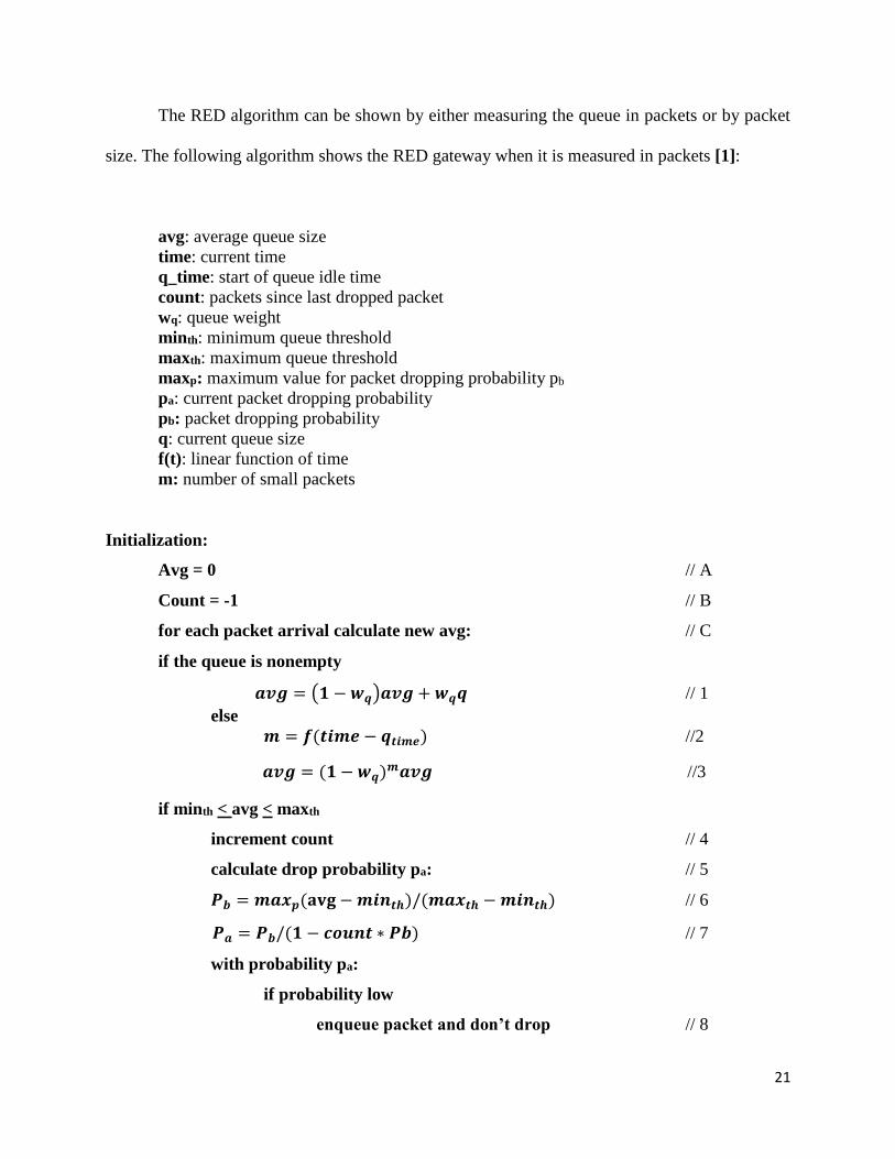
The RED algorithm can be shown by either measuring the queue in packets or by packet

size. The following algorithm shows the RED gateway when it is measured in packets [1]:

avg: average queue size

time: current time

q_time: start of queue idle time

count: packets since last dropped packet

wq: queue weight

minth: minimum queue threshold

maxth: maximum queue threshold

maxp: maximum value for packet dropping probability pb

pa: current packet dropping probability

pb: packet dropping probability

q: current queue size

f(t): linear function of time

m: number of small packets

Initialization:

Avg = 0 // A

Count = -1 // B

for each packet arrival calculate new avg: // C

if the queue is nonempty

𝒂𝒗𝒈 = (𝟏 − 𝒘𝒒)𝒂𝒗𝒈 + 𝒘𝒒𝒒 // 1

else

𝒎 = 𝒇(𝒕𝒊𝒎𝒆 − 𝒒𝒕𝒊𝒎𝒆) //2

𝒂𝒗𝒈 = (𝟏 − 𝒘𝒒)𝒎𝒂𝒗𝒈 //3

if minth < avg < maxth

increment count // 4

calculate drop probability pa: // 5

𝑷𝒃 = 𝒎𝒂𝒙𝒑(𝐚𝐯𝐠 − 𝒎𝒊𝒏𝒕𝒉)/(𝒎𝒂𝒙𝒕𝒉 − 𝒎𝒊𝒏𝒕𝒉) // 6

𝑷𝒂 = 𝑷𝒃/(𝟏 − 𝒄𝒐𝒖𝒏𝒕 ∗ 𝑷𝒃) // 7

with probability pa:

if probability low

enqueue packet and don’t drop // 8

22

else if probability high

randomly/linearly drop arriving packets // 9

count = 0

else if avg > maxth

drop all arriving packets // 10

count = 0

else count = -1

when queue becomes empty // 11

q_time = time // 12

Following is the explanation of the RED algorithm presented above [1]:

Initialize with the following statements:

A) The average queue size is zero

B) The queue is idle (empty)

C) Calculate the average queue size with L packet arrivals with the following formula:

𝒂𝒗𝒈𝑳 = 𝑳 + 𝟏 +(𝟏 − 𝒘𝒒)𝑳+𝟏 − 𝟏

𝒘𝒒

If the queue is not empty then

1) Use the formula following formula to calculate the average queue size avg

𝒂𝒗𝒈 = (𝟏 − 𝒘𝒒) 𝒂𝒗𝒈 + 𝒘𝒒𝒒

Else if the queue is empty (idle) then

2) Estimate the number of small packets m that could have been transmitted during the idle

period (to assist gateway with average queue size calculation) using the formula

𝒎 = 𝒇(𝒕𝒊𝒎𝒆 − 𝒒𝒕𝒊𝒎𝒆)

3) After the idle period the gateway computes the average queue size as if m packets had

arrived using the formula

𝒂𝒗𝒈 = (𝟏 − 𝒘𝒒)𝒎𝒂𝒗𝒈

If minth < avg < maxth then

23

4) Increase dropped packet count since last dropped packet

5) Calculate the final dropping probability pa

6) Calculate packet marking probability pb from that varies linearly from 0 to maxp as avg

varies from minth to maxth, using the formula


7) Calculation of final dropping probability by using the result of pb from #6

𝑷𝒂 = 𝑷𝒃/(𝟏 − 𝒄𝒐𝒖𝒏𝒕 ∗ 𝑷𝒃)

If packet dropping probability pa calculated in #7 is low then

8) Enqueue the packet and don’t drop

If packet dropping probability pa calculated in #7 is high and approaching maxth then

9) Randomly drop packets from connections and the count of packets since last drop is reset

to zero

Else if avg > maxth then

10) Drop all arriving packets and set count of packets since last drop to zero

Else count = -1 (i.e. avg < minth)

11) When the queue becomes empty

12) Time is reset to the start of the queue idle time

The only difference to be made to the RED algorithm in order to measure the queue by packet

size would be to replace the pb function of


with

𝑷𝒃 = 𝑷𝒃 ∗ 𝑷𝒂𝒄𝒌𝒆𝒕𝒔𝒊𝒛𝒆/𝑴𝒂𝒙𝒊𝒎𝒖𝒎𝑷𝒂𝒄𝒌𝒆𝒕𝑺𝒊𝒛𝒆

where, as mentioned before, the PacketSize is the size of the incoming packet in bytes and the

MaximumPacketSize is the maximum segment size in bytes the sender can transmit during that

particular RTT and pb varies between 0 and maxp [1][24]. Simulations performed on RED prove

24

that with the proper parameters, RED is successful at controlling congestion at the queue in

response to the change in load at the connections.

3.4 Simulations

3.4.1 RED Simulations

Floyd and Jacobson’s RED simulation in [1] shows that as the number of connections

linked to the gateway increase, the probability that packets will be dropped also increases. The

simulation network in Figure 4 contains four sources, each sending 1000-byte packets, linked to

the gateway and each with a maximum window size that ranges from 33 to 112 packets. The

parameters are set as follows: wq = 0.002, minth = 5 packets, maxth = 15 packets, and maxp =

1/50

Figure 4: RED simulation network where data transmission at node 1 starts at 0 seconds,

node 2 after 0.2 seconds, node 3 at 0.4 seconds and node 4 after 0.6 seconds

25

The simulation shows that by using RED at the gateway, the average queue size was successfully

controlled in response to changing load. The frequency at which packets were dropped increased

as the number of connections increased. Another key factor that shows RED’s success was the

fact that there was no global synchronization that led to continuous congestion at the gateway.

As a packet was dropped, RED was able to accommodate the burstiness in the queue required by

the slow-start phase [1]. Of all the four sources above, RED dropped a higher percentage of

packets from the node that had the largest input rate. For a short period of time if the assumption

is that the average queue size and the packet drop probability p remains the same and λi is the

connection’s input rate, then the formula for dropped packets from connectioni is as follows:

𝝀𝒊𝒑

∑𝝀𝒊𝒑=

𝝀

∑𝝀𝒊

Formula 5: Dropped packets from connectioni [15]

3.4.2 RED and Tail Drop comparison

In another simulation performed by Shu-Gang Liu in 2008, RED’s advantages against the

TD algorithm are showcased with the use of the NS-2 network simulator. The simulation

network in Figure 5 that Shu-Gang Liu used contains two routers and four connections as

follows [34]:

26

Figure 5: RED and TD comparison simulation network with a queue limit of 25 packets

between routers r1 and r2

Once the simulation is run, the results of TD and RED are compared in terms of delay where the

source ‘s2’ is used for the investigation. RED and TD were used between r1 and r2 to measure

the delay time between s2 and s4, respectively. Because the amount of congestion experienced

between the TD gateways is higher, the delay of the data packets travelling from s2 to s4 is also

higher. In Figure 6 and Figure 7 it can be observed that there is a significant difference in delay

times between TD and RED where the peak delay of TD is 170ms and for RED it is 110ms.

DELAY

Figure 6: TD with peak delay time of 170ms

27

Figure 7: RED with peak delay time of 110ms

3.4.3 RED and Random Drop comparison

In another simulation performed by Floyd in [1], the point of comparison was to prove

that RED is unbiased against bursty traffic unlike RD and TD. RED gateways differ from RD in

that RD’s mechanism does not contain a minimum and maximum threshold hence the most

appropriate comparison strategy is between both gateways that maintain the same average queue

size [14]. Figure 8 below shows the simulation network of four FTP sources where node 5 is

used in order to compare throughput, average queue and average link utilization. Node 5 has a

RTT that is 6 times that of other packets and contains a small window therefore packets that

arrive either arrive at the gateway with a long or many small interarrival times between them.

In this simulation the minimum threshold ranges from 3 to 14 packets, the maximum

threshold is 2 times the minimum threshold and the buffer size is 4 times the minimum threshold

28

which is therefore a range of 12 to 56 packets. The buffer size for RD ranges from 8 to 22

packets.

Figure 8: Simulation network comparing RED and

Random Drop

Because of node 5’s large RTT and small window, this puts node 5 as close to the maximum

throughput possible using a RED gateway. For node 5 a RTT that is six times longer than other

links means that the throughput will be less than with other links because of the amount of time a

packets takes to reach its destination and receive an ACK in return. The following maximum

TCP throughput formula proves that a larger RTT means that the throughput will be lower [26]:

𝐌𝐚𝐱 𝐓𝐂𝐏 𝐓𝐡𝐫𝐨𝐮𝐠𝐡𝐩𝐮𝐭 = 𝐑𝐂𝐕 𝐁𝐮𝐟𝐟𝐞𝐫 𝐒𝐢𝐳𝐞 / 𝐑𝐓𝐓

Formula 6: The throughput is measured in bits/second where RTT is calculated in this

formula as a fraction of a second. The larger the value for RTT, the lower the throughput

value will be where RCV Buffer Size is the receiver window buffer size of 65,535 bytes

29

With the RD gateway, node 5 receives only a small fraction of the throughput but a large fraction

of the packet drops. Considering the large RTT for node 5, node 5 still maintains a consistently

high throughput in comparison to RD as shown in Figure 9.

Figure 9: Comparison of throughput for Random Drop gateway on the left to the RED

gateway on the right using the same node

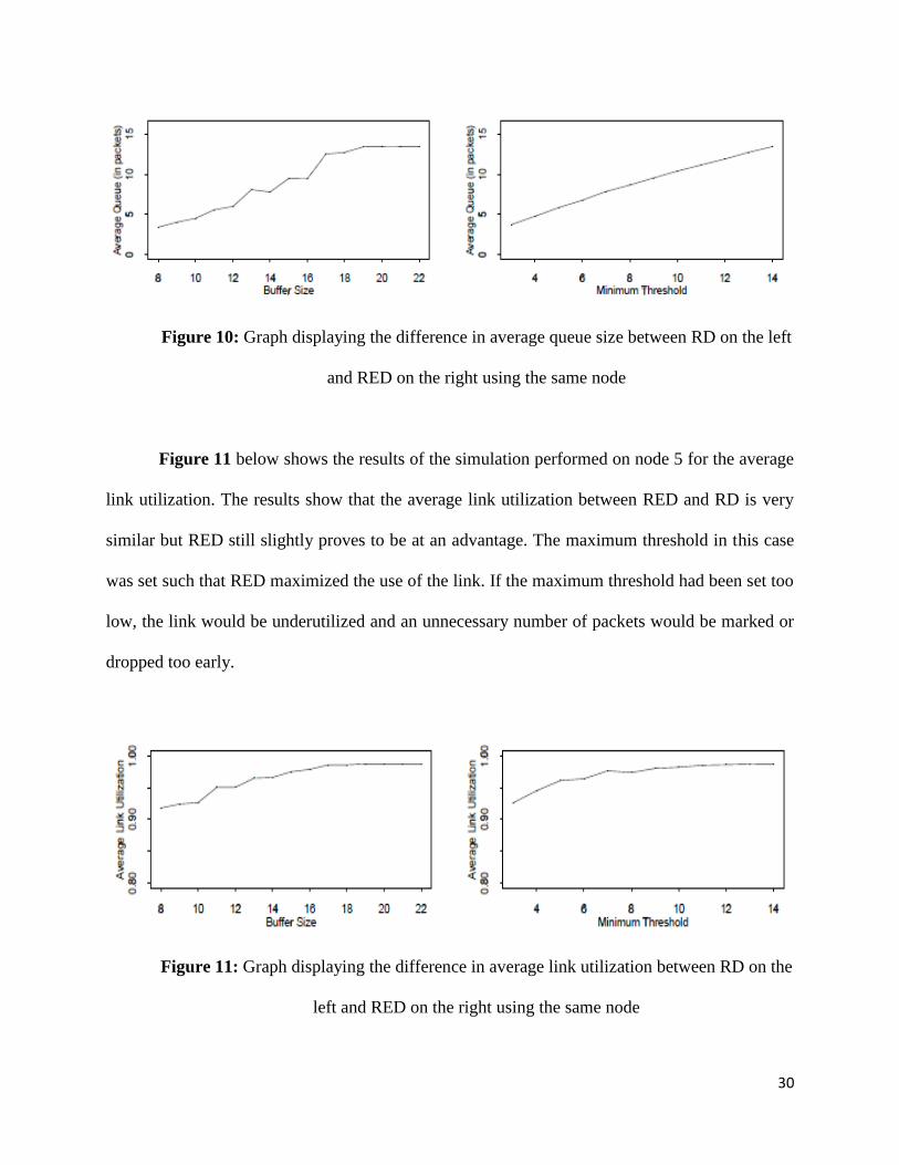
Figure 10 below displays RED’s advantage over RD in terms of the average queue in

packets. The average queue for RED is less than RD because it is unbiased against bursty traffic.

The average queue size for RED is measured with each packet sent out rather than instantaneous

as with RD therefore congestion is avoided earlier on rather than when the queue is already full.

30

Figure 10: Graph displaying the difference in average queue size between RD on the left

and RED on the right using the same node

Figure 11 below shows the results of the simulation performed on node 5 for the average

link utilization. The results show that the average link utilization between RED and RD is very

similar but RED still slightly proves to be at an advantage. The maximum threshold in this case

was set such that RED maximized the use of the link. If the maximum threshold had been set too

low, the link would be underutilized and an unnecessary number of packets would be marked or

dropped too early.

Figure 11: Graph displaying the difference in average link utilization between RD on the

left and RED on the right using the same node

31

4. Improvements to RED

4.1 Introduction

As mentioned earlier in this paper, the success of the RED algorithm in improving

throughput, delay, link utilization, packet loss rate and system fairness relies on the optimal

parameterization of its variables. In order for RED to be successful, these parameters must be set

in such a way that the RED mechanism can strike a balance between reducing packet loss and

preventing underutilization of the links by adjusting the rate of congestion notification [17]. RED

parameters that are not sufficiently aggressive can quickly degenerate the queues into a simple

TD queue. As the number of connections in a network increases, the impact of individual

congestion notifications decreases therefore in order for RED to be consistently effective in such

a situation, constant tuning of parameters would be required to adjust to current traffic situations.

This constant requirement to adjust RED parameters to adapt to the network conditions would be

an issue for network operators. Network operators require an estimation of the average delays in

their congested routers in order to improve delay times as a part of the QoS delivered to their

customers [37]. The following weaknesses of RED have caused the need for a tweak to the basic

RED algorithm:

1) Network operators require that the average queuing delay be predictable in advance. RED’s

average queuing delay is not easy to predict because its average queuing delay is sensitive to

the traffic load and parameters.

2) RED performs well when the average queue length is between the minimum and maximum

queue threshold but once avg is greater than maxth, RED does not perform as well, resulting

in decreased throughput and increased packet dropping rates.

32

As stated in [34], unless upgrades to network routers are deemed necessary, it’s unlikely that

network administrators would deploy the RED algorithm on routers of a core network as it can

be very complex and costly. Since the introduction of the concept of RED, many different

variations have been proposed that alleviates the issues faced with RED. The main variations of

RED are known to be Flow Random Early Detection (FRED), Weighted Random Early

Detection (WRED) and Adaptive Random Early Detection (ARED). Although more recently

many other variations and optimizations to RED have been proposed, neither have been

researched as extensively as FRED, WRED and ARED. More recent variations of RED have

further optimized their approach based on the ideas within the three main variations above.

Neither of the all the variations of RED resolves all of the issues that come with RED but rather

present a greater improvement in one or two main problem areas.

4.2 Weighted RED

WRED is a sophisticated algorithm that is currently implemented in routers of top tier-1

network equipment vendors such as Cisco and Juniper. WRED is advantageous over the original

RED algorithm in that it additionally provides early detection of congestion for multiple classes

of traffic. WRED drops packets from potentially congestive connections based on IP precedence

therefore packets with a lower IP precedence is more likely to be dropped than a packet with

higher IP precedence; non-IP traffic is more likely to be dropped than IP traffic [2][30].

Additionally, separate thresholds are provided for different IP precedences which mean that

different qualities of service are allowed for different traffic classifications, for example the port

number or protocol, with regards to packet dropping [2][22]. WRED provides early detection

33

with QoS differentiation unlike RED where the drop probability is based on the connection’s

share of the bandwidth.

4.2.1 Cisco WRED Configuration

4.2.1.1 Enabling WRED

The Cisco routing platforms that support the WRED feature are the ASR 100, ASR 920,

1700, 1800, 7000 and 12000 series. In global configuration mode in the Cisco IOS (Internetwork

Operating System), WRED must first be enabled on the router. Once WRED is enabled, the

default parameters are pre-set in order to control traffic of all precedences. The default

parameters are as follows [48][56]:

- Weight factor: used in order to calculate the average queue length and is set to 9

- Mark probability denominator: 10 (1 out of 10 packets are dropped once the average

queue reaches the maximum threshold)

- Maximum threshold: based on the output buffering capacity and the transmission speed

for the interface.

- Minimum threshold: IP Precedence 0 is calculated as half of the maximum threshold.

Other precedences oscillate between half the maximum threshold and the maximum

threshold.

The following commands are executed in interface configuration mode in order to enable WRED

with the default parameter values [55]:

COMMAND PURPOSE

Router(config)# interface type number Specifies the router interface type and number on

34

which to apply WRED

Router(config-if)# random-detect Enables WRED on the router with a weight factor

of 9 and mark probability denominator of 10

In order to modify the weight factor parameter along with the minimum and maximum threshold

values based on different IP precedences, the following optional commands can be executed in

interface configuration mode [48][55][56]:

COMMAND PURPOSE

Router(config)# interface type number Interface on which to configure WRED

Router(config-if)# random-detect

exponential-weighting-constant number

Enables WRED on the router with a specified

weight factor <number>

Router(config-if)# random-detect

precedence precedence min-threshold max-

threshold mark-prob-denominator

Specifies the minimum and maximum threshold

and the marking probability denominator for a

particular ip precedence <precedence>

Note: In order to configure RED instead of WRED, all precedences should be set with the same parameters

4.2.1.2 Configuring WRED in a Traffic Policy

A traffic policy can be created such that traffic classes can be included under this policy

and inherit the characteristics configured for this policy. The policy-map command is used to

create a traffic policy as shown in the following steps [47]:

COMMAND PURPOSE

Router(config)# policy-map policy-map Creates a traffic policy

Router(config-pmap)# class class-name Creates a traffic class to be included under the

traffic policy

Optional Step:

Router(config-pmap-c)# random-detect

exponential-weighting-constant number

Specifies a weight factor (other than the default

weight factor of 9)

Optional Step:

Router(config-pmap-c)# bandwidth

bandwidth-kbps

Specifies the amount of bandwidth assigned to

that traffic class (in kbps)

Optional Step:

Router(config-pmap-c)# fair-queue [queue-

limit queue-values

Specifies the maximum number of queues to

be allowed for that traffic class

35

Router(config-pmap-c)# queue-limit number-

of-packets

Specifies the maximum number of packets

allowed to be queued for that traffic class

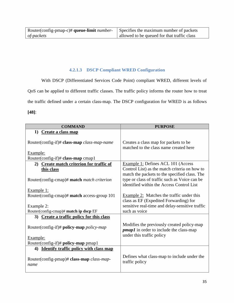
4.2.1.3 DSCP Compliant WRED Configuration

With DSCP (Differentiated Services Code Point) compliant WRED, different levels of

QoS can be applied to different traffic classes. The traffic policy informs the router how to treat

the traffic defined under a certain class-map. The DSCP configuration for WRED is as follows

[48]:

COMMAND PURPOSE

1) Create a class map

Router(config-if)# class-map class-map-name

Example:

Router(config-if)# class-map cmap1

Creates a class map for packets to be

matched to the class name created here

2) Create match criterion for traffic of

this class

Router(config-cmap)# match match criterion

Example 1:

Router(config-cmap)# match access-group 101

Example 2: Router(config-cmap)# match ip dscp EF

Example 1: Defines ACL 101 (Access

Control List) as the match criteria on how to

match the packets to the specified class. The

type or class of traffic such as Voice can be

identified within the Access Control List

Example 2: Matches the traffic under this

class as EF (Expedited Forwarding) for

sensitive real-time and delay-sensitive traffic

such as voice

3) Create a traffic policy for this class

Router(config-if)# policy-map policy-map

Example:

Router(config-if)# policy-map pmap1

Modifies the previously created policy-map

pmap1 in order to include the class-map

under this traffic policy

4) Identify traffic policy with class map

Router(config-pmap)# class-map class-map-

name

Defines what class-map to include under the

traffic policy

36

Example:

Router(config-pmap)# class-map cmap1

5) Identify allocated bandwidth for the

class

Router(config-pmap-c)# bandwidth bandwidth-

kbps

Example:

Router(config-pmap-c)# bandwidth 2000

Defines how much bandwidth is allocated to

that class

6) Specify DSCP based packet dropping

Router(config-pmap-c)# random-detect dscp-

based

Note: If not already specified in step 2

Specifies that WRED should use the DSCP

value for drop probability calculation

7) Specify the DSCP value

Router(config-pmap-c)# random-detect dscp

dscpvalue min-threshold max-threshold

Example:

Router(config-pmap-c)# random-detect dscp 46

30 60

Note: If not already specified in step 2

Specifies the DSCP value 46, minimum

threshold of 30 and maximum threshold of

60 for packet drop probability

Note: DSCP value 46 is for VoIP voice

traffic

8) Specify which interface to apply the

traffic policy

Router(config)# interface interface name

Router(config-if)# service-policy output policy-

map

Example:

Router(config)# interface seo/0

Router(config-if)# service-policy output pmap1

Defines the output interface seo/0 for which

this traffic policy pmap1 should apply to

4.2.2 Cisco WRED Implementations

DSCP-based WRED is implemented on the Voice, Interactive Video, Streaming Video,

Transactional Data and Best Effort classes in order to manage and classify network traffic. The

forwarding classes that apply to each class are shown in Table 1 below [46][58]:

37

CLASS NAMES

FORWARDING CLASSES

Name (Per-hop behavior) based

DSCP based

value

VOICE EF 46

INTERACTIVE VIDEO AF41 34

STREAMING VIDEO AF31 26

TRANSACTIONAL DATA AF21 18

BULK DATA AF11 10

Table 1: Cisco Traffic classes with PHB and DSCP values

Once WRED is configured on the router for a certain traffic class, either the PHB (Per-hop

behavior) value or the dscp value must be matched against once the class-map and traffic policy

is created [46][47][48]. The following details WRED implementations in the traffic classes along

with configuration examples:

1) Voice: The WRED implementation in the Voice class is for VoIP telephony and is

assigned with an EF (Expedited Forwarding) PHB. Traffic assigned under the EF

building block should be of low delay, low jitter and low loss services. The following

configuration example for VoIP telephony uses class-based dropping and inspects all

incoming traffic through Ethernet 0/1 to be matched against the class-map VOIP which

contains the dscp value of 46 (Expedited Forwarding) [44][45]:

class-map match-all VOIP

!

policy-map dscp_marking

class voip

set ip dscp 46

!

interface Ethernet0/1

service-policy input dscp_marking

38

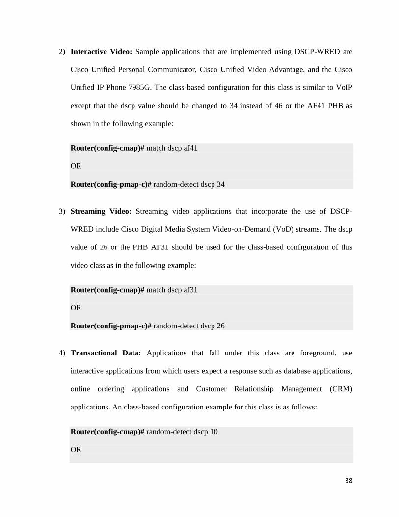
2) Interactive Video: Sample applications that are implemented using DSCP-WRED are

Cisco Unified Personal Communicator, Cisco Unified Video Advantage, and the Cisco

Unified IP Phone 7985G. The class-based configuration for this class is similar to VoIP

except that the dscp value should be changed to 34 instead of 46 or the AF41 PHB as

shown in the following example:

Router(config-cmap)# match dscp af41

OR


3) Streaming Video: Streaming video applications that incorporate the use of DSCP-

WRED include Cisco Digital Media System Video-on-Demand (VoD) streams. The dscp

value of 26 or the PHB AF31 should be used for the class-based configuration of this

video class as in the following example:

Router(config-cmap)# match dscp af31

OR


4) Transactional Data: Applications that fall under this class are foreground, use

interactive applications from which users expect a response such as database applications,

online ordering applications and Customer Relationship Management (CRM)

applications. An class-based configuration example for this class is as follows:

Router(config-cmap)# random-detect dscp 10

OR

39

Router(config-pmap-c)# random-detect dscp af11 40 60

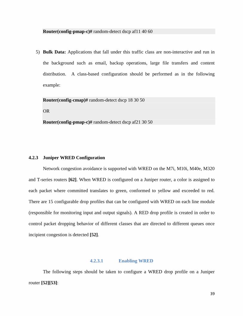
5) Bulk Data: Applications that fall under this traffic class are non-interactive and run in

the background such as email, backup operations, large file transfers and content

distribution. A class-based configuration should be performed as in the following

example:

Router(config-cmap)# random-detect dscp 18 30 50

OR

Router(config-pmap-c)# random-detect dscp af21 30 50

4.2.3 Juniper WRED Configuration

Network congestion avoidance is supported with WRED on the M7i, M10i, M40e, M320

and T-series routers [62]. When WRED is configured on a Juniper router, a color is assigned to

each packet where committed translates to green, conformed to yellow and exceeded to red.

There are 15 configurable drop profiles that can be configured with WRED on each line module

(responsible for monitoring input and output signals). A RED drop profile is created in order to

control packet dropping behavior of different classes that are directed to different queues once

incipient congestion is detected [52].

4.2.3.1 Enabling WRED

The following steps should be taken to configure a WRED drop profile on a Juniper

router [52][53]:

40

COMMAND PURPOSE

host1(config)#drop-profile name Creates drop profile <name>

host1(config-drop-profile)# Enter Drop profile configuration mode

host1(config-drop-profile)#average-length-

exponent 9 Sets the weight factor for the drop profile

Optional Step:

host1(config-drop-profile)#committed-

threshold percent 30 90 4

Sets the <minthreshold> <maxthreshold> <drop

probability> respectively, for committed traffic

Optional Step:

host1(config-drop-profile)#conformed-

threshold percent 25 90 5


probability> respectively, for conformed traffic

Optional Step:

host1(config-drop-profile)#exceeded-threshold

percent 20 90 6


probability> respectively, for exceeded traffic

4.2.3.2 Configuring WRED in a Traffic Policy

CoS (Class of Service) is configured on a device because special treatment must be

provided to different traffic classes with delay-sensitive traffic such as VoIP. Once packets arrive

on an interface, a buffer is required in order to queue these packets before they are forwarded.

There are two default queues used on Juniper devices which are Queue 0 for best effort delivery

and Queue 3 for network control traffic. The remaining two queues that can be configured are

Queue 1 (Expedited forwarding traffic) and Queue 2 (Assured forwarding traffic) [57].

FORWARDING CLASS OUTPUT QUEUE TRAFFIC TYPE

be-class Queue 0 Best effort traffic

ef-class Queue 1 Expedited forwarding traffic

af-class Queue 2 Assured forwarding traffic

nc-class Queue 3 Network control traffic

Table 2: Juniper Forwarding Classes and Output Queues

A forwarding class must be mapped to its appropriate queue in order to direct packets into the

correct queues once incipient congestion occurs; voice would be mapped to Queue 2. The

41

purpose of the scheduler is to determine how traffic received in that queue is treated [49][55].

The scheduler map maps the scheduler to its appropriate queue and the scheduler map must then

be associated with a traffic control profile [51]. A traffic control profile is used in order to set the

bandwidth of the output queue by defining how queues that are mapped to a forwarding class set

can share the bandwidth resources [50].

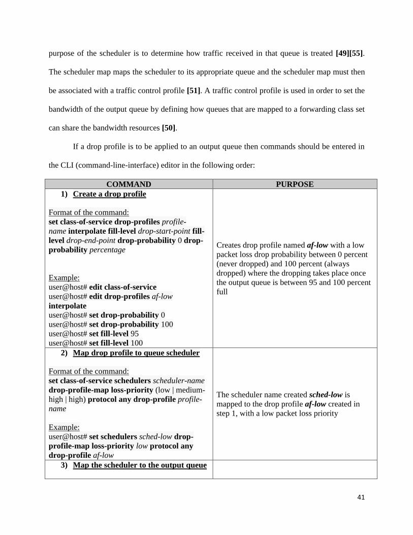
If a drop profile is to be applied to an output queue then commands should be entered in

the CLI (command-line-interface) editor in the following order:

COMMAND PURPOSE

1) Create a drop profile

Format of the command:

set class-of-service drop-profiles profile-

name interpolate fill-level drop-start-point fill-

level drop-end-point drop-probability 0 drop-

probability percentage

Example:

user@host# edit class-of-service

user@host# edit drop-profiles af-low

interpolate

user@host# set drop-probability 0

user@host# set drop-probability 100

user@host# set fill-level 95

user@host# set fill-level 100

Creates drop profile named af-low with a low

packet loss drop probability between 0 percent

(never dropped) and 100 percent (always

dropped) where the dropping takes place once

the output queue is between 95 and 100 percent

full

2) Map drop profile to queue scheduler


set class-of-service schedulers scheduler-name

drop-profile-map loss-priority (low | medium-

high | high) protocol any drop-profile profile-

name

Example:

user@host# set schedulers sched-low drop-

profile-map loss-priority low protocol any

drop-profile af-low

The scheduler name created sched-low is

mapped to the drop profile af-low created in

step 1, with a low packet loss priority

3) Map the scheduler to the output queue

42


set class-of-service scheduler-maps map-

name forwarding-class forwarding-class-

name scheduler scheduler-name

Example:

user@host# set class-of-service scheduler-

maps schedMap-Low forwarding-class af-

class scheduler sched-low

The forwarding class is now mapped to the low

packet loss priority queue, af-class, which is

mapped to the scheduler sched-low via the

scheduler-map schedMap-low

4) Relate the scheduler map to a traffic

profile:


set class-of-service traffic-control-profiles tcp-

name scheduler-map map-name

Example:

user@host# set class-of-service traffic-control-

profiles tcp-network scheduler-map schedMap-

Low

The scheduler map schedMap-Low is now

associated with the traffic profile tcp-network

5) Set the minimum and maximum

guaranteed bandwidth for the traffic

profile:


user@host# edit traffic-control-profiles tcp-

name guaranteed-rate Gigabytes

user@switch# edit traffic-control-profiles tcp-

name shaping-rate Gigabytes

Example:

user@host# edit traffic-control-profiles tcp-

network guaranteed-rate 2g

user@switch# edit traffic-control-profiles tcp-

network shaping-rate 4g

The minimum guaranteed bandwidth for traffic

entering this queue, under the traffic profile tcp-

network, and linked to scheduler shed_low is 2

gigabytes and the maximum is 4 gigabytes

6) Relate an interface with the traffic

control profile:


set class-of-service interface interface-

name forwarding-class-set forwarding-class-

set-name output-traffic-control-profile tcp-

name

Example:

The traffic control profile tcp-network is now

associated with the interface xe-0/0/1 unit 0

http://www.juniper.net/techpubs/en_US/junos13.2/topics/reference/configuration-statement/traffic-control-profiles-edit-class-of-service.html

http://www.juniper.net/techpubs/en_US/junos13.2/topics/reference/configuration-statement/guaranteed-rate-edit-class-of-service.html

http://www.juniper.net/techpubs/en_US/junos13.2/topics/reference/configuration-statement/shaping-rate-edit-class-of-service.html

http://www.juniper.net/techpubs/en_US/junos13.2/topics/reference/configuration-statement/traffic-control-profiles-edit-class-of-service.html

http://www.juniper.net/techpubs/en_US/junos13.2/topics/reference/configuration-statement/guaranteed-rate-edit-class-of-service.html

http://www.juniper.net/techpubs/en_US/junos13.2/topics/reference/configuration-statement/shaping-rate-edit-class-of-service.html

43

set class-of-service-interface xe-0/0/1 unit

1 forwarding-class-set af-set output-traffic-

control-profile tcp-network

4.2.4 Juniper WRED Implementations

WRED is implemented on the same traffic classes as with Cisco except that the

configuration on the routers and switches for these particular classes is slightly different. The

following configuration example details steps for a router on how voice traffic (VoIP) is given a

strict high priority over traffic coming into other queues. If another traffic class is to be added to

this configuration, its packet loss priority, IP precedence and forwarding class must be

configured accordingly such that voice traffic is given higher priority.

1) Using a classifier [59][61]: For every incoming packet, a classifier will decide what

output queue to forward the packet based on its forwarding class (FC). Once the packet is

forwarded to the appropriate output queue, the queue is then managed based on the

packet’s PLP (packet loss priority). There are two types of classifiers that can be used:

Behavior Aggregate (BA) and Multifield (MF); the BA classifier is the easiest way

within Juniper devices to classify packets. For this example, the BA classifier will be

used in order to set the forwarding class of an incoming packet based on a defined IP

precedence. Unless specified otherwise, the default classifier will classify the incoming

packet based on IP precedence.

set class-of-service classifiers inet-precedence classify_voice forwarding-class voice-class

loss-priority low code-points 010

44

IP PRECEDENCE

(Code Point)

FORWARDING

CLASS

PACKET LOSS

PRIORITY

000 Best-effort Low

001 Best-effort High

010 Best-effort Low


100 Best-effort Low


110 Best-effort Low


Table 3: Juniper IP Precedence classifier

The default IP precedence classifier can be overwritten in order to classify incoming

packets using a DSCP BA classifier in the following way:

set class-of-service classifiers dscp ba-classifier

set import default

set forwarding-class voice-class loss-priority low code-points 101110 #EF-class

set interfaces ge-0/0/1 unit 0 classifiers ba-classifier

The code points selection when using the DSCP classifier is based on the following

information:

DSCP Code

Points

MAPPING

ef 101110

af11 001010

af12 001100

af13 001110

af21 010010

af22 010100

af23 010110

af31 011010

af32 011100

af33 011110

af41 100010

af42 100100

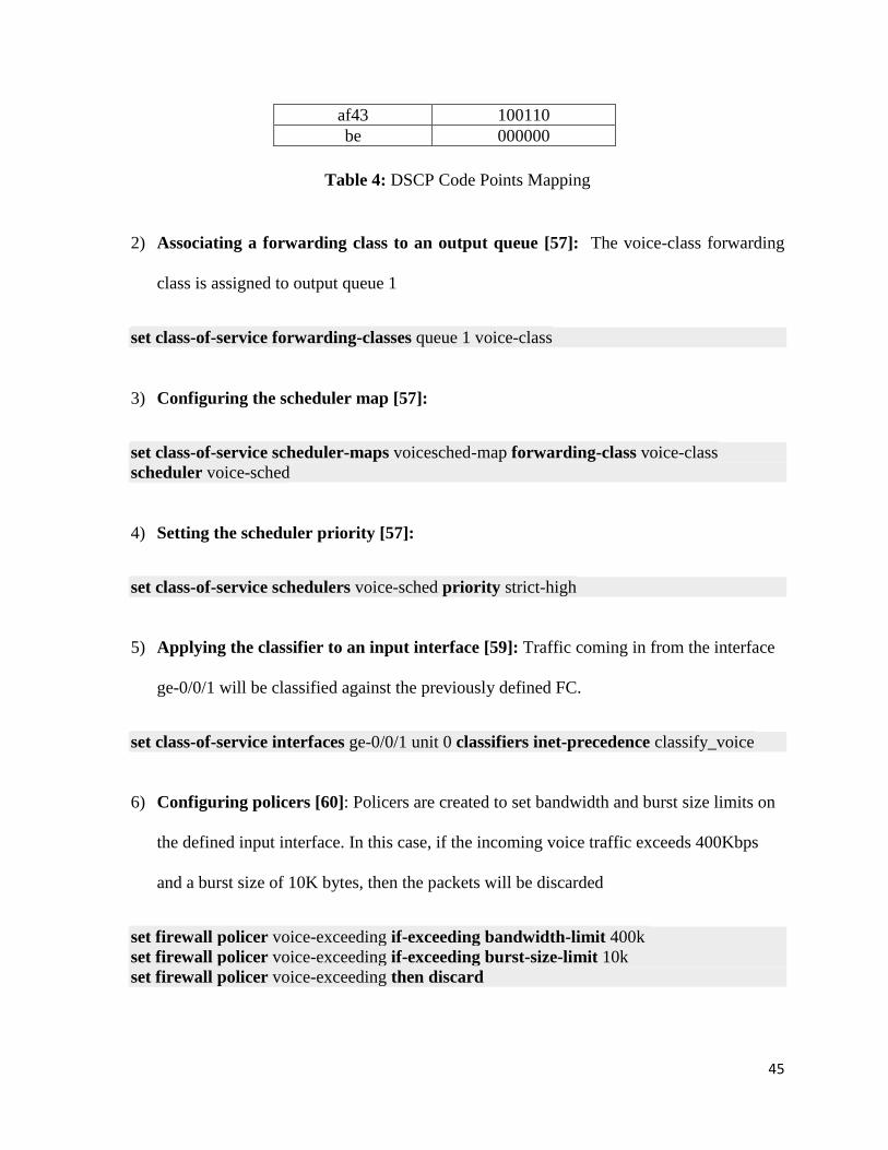
45

af43 100110

be 000000

Table 4: DSCP Code Points Mapping

2) Associating a forwarding class to an output queue [57]: The voice-class forwarding

class is assigned to output queue 1

set class-of-service forwarding-classes queue 1 voice-class

3) Configuring the scheduler map [57]:

set class-of-service scheduler-maps voicesched-map forwarding-class voice-class

scheduler voice-sched

4) Setting the scheduler priority [57]:

set class-of-service schedulers voice-sched priority strict-high

5) Applying the classifier to an input interface [59]: Traffic coming in from the interface

ge-0/0/1 will be classified against the previously defined FC.

set class-of-service interfaces ge-0/0/1 unit 0 classifiers inet-precedence classify_voice

6) Configuring policers [60]: Policers are created to set bandwidth and burst size limits on

the defined input interface. In this case, if the incoming voice traffic exceeds 400Kbps

and a burst size of 10K bytes, then the packets will be discarded

set firewall policer voice-exceeding if-exceeding bandwidth-limit 400k

set firewall policer voice-exceeding if-exceeding burst-size-limit 10k

set firewall policer voice-exceeding then discard

46

7) Creating a firewall filter [61]: Firewall filters can optionally be configured so that the

router and/or switch can be protected from excessive traffic going through the router. In

this case, the new policers created are now included under the firewall filter configuration

to control traffic transiting the router. The next term command informs the router to use a

next defined term in the configuration to perform configured actions on the incoming

packet.

set firewall filter voice-term term 01 from forwarding-class voice-class

set firewall filter voice-term term 01 then policer voice-exceeding

set firewall filter voice-term term 01 then next term

4.3 Flow RED

FRED is an extension of WRED and its goal is to reduce the unfairness effects found in the

original design of RED by generating selective feedback to a filtered set of connections which

have a large number of packets queued [15]. The issue with FRED is that it presents a substantial

departure from the original RED design with the introduction of additional parameters. These

parameters include minq and maxq (minimum and maximum number of packets allowed to be

buffered for each flow), avgcq (average per-flow buffer count), qlen (count of buffered packets

per flow) and strike count for the number of times a flow hasn’t responded to congestion

notification. In FRED, the calculation of the average queue length is performed at both the

arrival and the departure of the packets [15]. Currently WRED is more widely implemented on

gateway routers than its FRED extension. If the need for FRED is identified, the algorithm can

be configured but in order to do so network engineers must first enable and configure WRED on

the router before FRED can be enabled.

47

4.4 Adaptive RED

The goal of discussing a new version of RED in this paper is to stay as close to the

original RED algorithm as possible because most of the other variations of RED represent

substantial departures from the basic RED design. The revised RED algorithm called ARED

achieves the desired target queue length without sacrificing other benefits of RED, can be

implemented with a simple extension, proves to be sufficiently robust and can be automatically

parameterized [37]. RED routers that show promise in easier configuration and parameterization

prove to be more robust for deployment in routers. Adaptive RED (ARED) can be implemented

as a simple extension to the basic RED algorithm and removes sensitivity to parameterization

making it more worthwhile for deployment in routers [34][35].

RED parameters are statically coded in its algorithm but ARED’s variables are more

dynamic such that initially only the minth variable needs to be set, then the coding within the

algorithm will automatically set the other values as in Formula 7 below:

C = link Capacity in packets/second computed for packets of the specified default size

𝒘𝒒 = 𝟏 − 𝐞𝐱𝐩 (−𝟏/𝑪)

Formula 7: ARED algorithm weighted moving average

In auto mode, once the minth value is set, the target queue size is 2 x minth and maxth is

3 x minth. With the proposal in [35], Floyd et al adjusts the upper bound on the dropping

probability maxp such that the average queue size is kept between the minth and maxth values; the

average queue size stays close to the target queue size. The operator, therefore, needs only to set

48

the target average queue length required. Simulations performed by Feng et al and Floyd et al in

[17][19][35] prove the following:

1) The stability of a network with RED gateways and TCP connections depend on the load of

the network but does not for an ARED network.

2) RED is sensitive not only to the parameters but also to the RTT’s of the connections. In

simulations performed in ns-2, ARED exhibits less sensitivity in both of these regards.

Both of the above advantages of ARED come with the disadvantage that the input of the target

queue size beforehand means that there is a tradeoff between small queuing delay and stability as

proven in [36]. Figure 12 below demonstrates how the ARED algorithm functions [19]:

Figure 12: ARED algorithm diagram

49

ARED compares the average queue size to the target queue size every ∆𝒊𝒏𝒕𝒆𝒓𝒗𝒂𝒍 amount of time.

If by the end of the ∆𝒊𝒏𝒕𝒆𝒓𝒗𝒂𝒍 of time if the average queue size is greater than the target queue

size and maxp < 0.5, then maxp is increased by 𝜶𝒂𝒓𝒆𝒅 which is greater than 0. If the average

queue size is less than the target queue size and maxp > 0.01, then maxp is multiplied by 𝜷𝒂𝒓𝒆𝒅

which is less than 1 [36].

It is not claimed that ARED resolves all issues faced with RED but it is deemed more

attractive than other versions of RED because it is less sensitive to parameterization and requires

minimal change to the original RED design. Currently ARED is not implemented on any routers.

50

5. Conclusion

The research detailed in this paper shows that congestion can successfully be avoided at

the gateway with the cooperation of a transport protocol such as TCP. The mechanism of

dropping packets once they reach a maximum threshold has been shown to be effective for

controlling the average queue size. RED is unbiased against bursty traffic because the probability

for RED to drop a packet from a connection is proportional to that connection’s share of the

bandwidth. If a small portion of the bandwidth is used by a bursty connection, the connection is

not penalized by RED unlike Tail Drop and Random Drop and in this sense RED is more fair.

RED also avoids global synchronization since the drop probability is proportional to the flow’s

share of the bandwidth. Since not all connections use the exact share of the bandwidth in one

instance, not all flows slow down the transmission of their data at the same time. Flows enter the

congestion avoidance state at different time intervals, avoiding the global synchronization by

RED dropping packets at the lowest possible rate.

The Network Working Group (NTWG) recommends the use of RED based on the fact

that unless network engineers have a better mechanism for congestion avoidance, RED has

proven to perform an above decent job at managing queue lengths, reducing end-to-end latency,

reducing packet dropping and avoiding the lock-out phenomena [16]. RED does also come with

some flaws as a result of networks continually becoming more demanding in terms of the need

for increased RTTs.

One of the improvements to RED has been to improve fariness by calculating the average

queue length with the arrival plus the departure of a packet; called FRED. One of the most

notable developments to RED has been the addition of resource management to routers such that

51

different traffic classes would be provided with different drop priorities, proposed by the WRED

algorithm. WRED has been shown to be the most widely implemented algorithm within tier-1

vendor routers and it can be easily configured on network devices. ARED provides a simple

extension to the basic RED design and shows promise of adaptability to various network

conditions by setting a target queue length and with the ability to dynamically parameterize its

variables. The success of RED lies in the optimal parameterization of its variables in order to

accommodate changing network conditions otherwise it can quickly degrade to the behavior of a

TD and RD algorithm.

52

6. Future work

The future work involved for the RED algorithm focuses on optimizing the average

queue size in order to maximize the throughput and minimize the delay [1]. RED parameters

should adapt to different network loads including that of demanding wireless links therefore

should be dynamically rather than statically tuned. Such self-tuning RED algorithms still do not

change the basic principles of RED therefore more research needs to be performed into the RED

algorithm under more aggressive network conditions with multiple bottlenecks and multiple

links of varying bandwidths. As a bulk of the research on RED is based on RED’s behavior

within a TCP network, future work should include the same amount of research with transport

protocols other than TCP in order to evaluate its efficiency in various traffic conditions with

more aggressive parameters. There are also connections that are unresponsive to congestion

notification that may propose issues in a network therefore research may be continued on the

RED mechanism for the handling of such flows [16]. New proposals on variations of the RED

algorithm should be kept as simple as possible whilst optimizing or providing small extensions to

the original algorithm.

53

Glossary

Active open call: the first state the client must be in to initiate a connection with the server

by sending a Synchronize (SYN) message to the server

Acknowledgement (ACK): The message that the receiver sends back to the sender in order

to acknowledge the receipt of the data packet received

Bit errors: occur when packets are transmitted and some of the bits within the packet are

modified

Buffer: an area within the physical memory storage of a device, such as a router, where data

is stored temporarily before it is transferred to the next device

Bursty traffic: a bulk of data sent or received in one intermittent transmission

Congestion: occurs on a network when a device, such as a router, is receiving more packets

than it can handle

Congestion control: technique that is used to ameliorate congestion, by ensuring that a

single connection cannot consume all of the available bandwidth

Delay: specifies how long it takes for data packets to travel from a sender to a receiver on a

network

Fairness: specifies whether applications and/or devices are receiving a fair share of network

resources.

Fast Retransmit: the sender immediately transmits the missing segment to the waiting

receiver and half of the current congestion window cwnd is saved as slow-start threshold

ssthresh

54

Fast Recovery: performed by the sender right after a Fast Retransmit by maintaining the

same larger window size but slowing down transmission and increasing window size linearly

hence entering the congestion avoidance state

Full-duplex transmission: bidirectional transmission of data between two nodes

Full-queue problem: when queues fill up fast because no indication of congestion is

provided to the sources and congestion control is initiated once the queue is almost or already

full

Global synchronization: pattern of all TCP/IP connections simultaneously starting and

stopping their transmission of data during periods of congestion

Initial Sequence Number (ISN): first sequence number in the Sequence field of the TCP

Header

Internet Protocol (IP): resides in the network layer and handles the addressing for the

transmission of data packets to ensure that they are sent to the correct destination

Lock-out problem: flows unfairly occupying a very large portion of the bandwidth caused

by global synchronization

Memory buffer: buffer included in TCP that is situated between the application layer and

the data link layer that is responsible for receiving the data. The memory buffer, therefore,

allows data to be independently received and read from the application layer while the

application layer is allowed to process data at its own pace.

Maximum Segment Size (MSS): largest segment that the sender can transmit at one time

Network power: ratio of throughput to delay in a network

Passive open call: the state that the server must be in to inform the client that it is waiting for

an active open call from the client

55

Piggybacking: when an ACK is appended to a data frame and sent at the same time such that

it ‘piggybacks’

Proactive Packet Discard: when routers are enhanced to detect and notify connections of

impending congestion earlier, allowing them to slow down their transmission rates before the

router buffer overflows

Quality of Service (QoS): refers to the prioritization provided to certain delay and time-

sensitive applications such that there is a guarantee of agreed services catered to that data

flow over lower priority flows

Queue law: a router queue at equilibrium has an average queue length as a function of the

packet drop probability

Round Trip Time (RTT): time calculated between the clocking in of the first bit of data

sent and the receipt of the corresponding ACK received

Slow-start algorithm: ‘Sliding window’ technique used at the start of a new connection or

when restarting segment transmission from a connection that has timed out. The growth of

the number of packet segments sent grows exponentially with the successful receipt of the

same number of ACKs in return

Three-Way Handshake: the connection establishment that occurs between the client and

server such that certain messages are sent and acknowledged before any data transfer can

occur

Throughput: the rate at which packets are successfully delivered in a given period of time

Timeout: one of the ways TCP detects congestion and occurs when the sender does not

receive an ACK within the calculated time of the RTT and connections are forcefully closed

56

Transmission Control Protocol (TCP): used as the core protocol or set of rules in the

transport layer to deliver packets in a reliable manner from an application program over the

Internet using the Internet Protocol (IP)

Voice-over-IP (VoIP): refers the methodology that makes use of the Internet Protocol (IP) to

transport voice data over a network

Window size: receiving capacity in terms of bytes (segment size)

57

References

[1] S. Floyd and V. Jacobson. (1993, Aug.). Random Early Detection Gateways for Congestion

Avoidance. IEEE/ACM Transactions on Networking, CA, USA. [Online] p. 1 Available:

http://www.icir.org/floyd/papers/early.twocolumn.pdf

[2] Cisco. Configuring Weighted Random Early Detection. Cisco, CA, USA. [Online] Available:

http://www.cisco.com/en/US/docs/ios/12_2/qos/configuration/guide

/qcfwred_ps1835_TSD_Products_Configuration_Guide_Chapter.html#wp1005223

[3] H. Balakrishnan, V.N. Padmanabhan et al. (1997). A comparison of mechanisms for

improving TCP performance over wireless links. IEEE/ACM Transactions on Networking, CA,

USA. [Online] p. 1 Available: http://daedalus.cs.berkeley.edu/publications/sigcomm96.pdf

[4] D. Bunitas. (1995, Aug.). Congestion Control Schemes for TCP/IP Networks. [Online]

Available: http://www.cse.wustl.edu/~jain/ cis788-95/ftp/tcpip_cong/#REDolumn.pdf

[5] G. Davis, D. Rolf. (2009, Dec.). Advantages in Network Efficiency offered by Weighted

RED (WRED). UTAS, CA, USA. [Online] Available:

https://enterprise1.opnet.com/tsts/4dcgi/Biblio_FullAbstract?BiblioID=1612

[6] H. Balakrishnan, S. Seshan et al. (1995, Nov.). Improving TCP/IP performance over wireless

networks. 1st ACM conf. on mobile computing and networking, CA, USA. [Online] p.1

Available:

http://citeseerx.ist.psu.edu/viewdoc/download?doi=10.1.1.182.1106&rep=rep1&type=pdf

[7] S. Floyd. (1997). RED: Discussions of Setting Parameters. [Online] Available:

http://www.icir.org/floyd/REDparameters.txt

http://www.icir.org/floyd/papers/early.twocolumn.pdf

http://www.cisco.com/en/US/docs/ios/12_2/qos/configuration/guide%20/qcfwred_ps1835_TSD_Products_Configuration_Guide_Chapter.html%23wp1005223

http://www.cisco.com/en/US/docs/ios/12_2/qos/configuration/guide%20/qcfwred_ps1835_TSD_Products_Configuration_Guide_Chapter.html%23wp1005223

http://daedalus.cs.berkeley.edu/publications/sigcomm96.pdf

http://www.cse.wustl.edu/~jain/%20cis788-95/ftp/tcpip_cong/%23REDolumn.pdf

https://enterprise1.opnet.com/tsts/4dcgi/Biblio_FullAbstract?BiblioID=1612

http://citeseerx.ist.psu.edu/viewdoc/download?doi=10.1.1.182.1106&rep=rep1&type=pdf%20

http://www.icir.org/floyd/REDparameters.txt

58

[8] T. Ziegler, C. Brandauer et al. (2001) Stability Criteria of RED with TCP Traffic. 9th IFIP

Conference on Performance Modeling and Evaluation of ATM and IP Networks, HU. [Online]

Available: http://www.salzburgresearch.at/~cbrand/pub/report_redstability_00.pdf

[9] G. Iannaccon, C. Brandauer et al. Comparison of Tail Drop and Active Queue Management

Performance for bulk-data and Web-like Internet Traffic, Austria. [Online] Available:

https://research.sprintlabs.com/publications/uploads/ieeescc01_ziegler.pdf

[10] M. Allman, V. Paxson et al. (2009, Sept.). TCP Congestion Control. Network Working

Group. [Online] Available: http://tools.ietf.org/html/rfc5681

[11] K. Ramakrishnan, S. Floyd et al. (2001, Sept.). The Addition of Explicit Congestion

Notification (ECN) to IP. Network Working Group. [Online] Available:

http://tools.ietf.org/html/rfc3168

[12] V. Paxson, M. Allman et al. (2000, Nov.). Computing TCP’s Retransmission Timer.

Network Working Group. [Online] Available: http://tools.ietf.org/html/rfc2988

[13] S. Floyd. (1994, Oct.) TCP and Explicit Congestion Notification. ACM SIGCOMM

Computer Communication Review, NY, USA. [Online] Available:

http://www.icir.org/floyd/papers/tcp_ecn.4.pdf

[14] E.S. Hashem. (1989, Aug.). Analysis of Random Drop for Gateway Congestion Control,

MA, USA. [Online] Available: www.dtic.mil/cgi-bin/ GetTRDoc? AD =ADA218737

[15] D. Lin and R. Morris. (1997). Dynamics of Random Early Detection, MA, USA. [Online]

Available: http://pdos.csail.mit.edu/rtm/papers/fred.pdf

http://www.salzburgresearch.at/~cbrand/pub/report_redstability_00.pdf

https://research.sprintlabs.com/publications/uploads/ieeescc01_ziegler.pdf




http://www.icir.org/floyd/papers/tcp_ecn.4.pdf

http://www.dtic.mil/cgi-bin/%20GetTRDoc?%20AD%20=ADA218737

http://pdos.csail.mit.edu/rtm/papers/fred.pdf

59

[16] B. Braden, D. Clark et al. (1998, April.). Recommendations on Queue Management and

Congestion Avoidance in the Internet. Network Working Group. [Online] Available:


[17] W. Feng, D. Kandlur. (1999, March). A Self Configuring RED Gateway. INFOCOM '99.

Eighteenth Annual Joint Conference of the IEEE Computer and Communications Societies, NY,

USA. [Online] Available: http://debanjan.sahafamily.com/papers/ 00752150.pdf

[18] J. Chung. (2003, April). Analysis of Active Queue Management. Network Computing and

Applications, MA, USA. [Online] Available: web.cs.wpi.edu/~claypool/papers/queue -law/aqm-

analysis.pdf

[19] R. J. La, P. Ranjan. (1993). Analysis of Adaptive RED (ARED), MD, USA. [Online]

Available: http://www.ece.umd.edu/~hyongla/PAPERS/ITC03_ared.pdf

[20] C. Brandauer. (2000). Stability Criteria of RED with TCP Traffic. Salzburg Research.

[Online] Available: http://www.salzburgresearch.at/~cbrand/pub/report_redstability_00.pdf

[21] W. Stevens, NOAO. (1997, Jan.). TCP Slow Start, Congestion Avoidance, Fast Retransmit,

and Fast Recovery Algorithms. Network Working Group. [Online] Available:


[22] N. Hamadneh, D. Murray et al. (2012). Dynamic Weight Parameters for Random Early

Detection (RED) in TCP Networks. International Journal on New Computer Architectures and

Their Applications, AUS. [Online] Available:

http://sdiwc.net/digitallibrary/download.php?id=00000178.pdf

[23] S. Floyd and V. Jacobson. (1991, April). On Traffic Phase Effects in Packet-Switched

Gateways. ACM SIGCOMM Computer Communication Review, NY, USA. [Online] Available:

http://www.icir.org/floyd/papers/phase.pdf


http://debanjan.sahafamily.com/papers/%2000752150.pdf

http://www.ece.umd.edu/~hyongla/PAPERS/ITC03_ared.pdf

http://www.salzburgresearch.at/~cbrand/pub/report_redstability_00.pdf


http://sdiwc.net/digitallibrary/download.php?id=00000178.pdf

http://www.icir.org/floyd/papers/phase.pdf

60

[24] M. Burghout. (2008, June). Experimental Analysis of the impact of RTT differences on the

throughput of two competing TCP flows, NL. [Online] Available:

http://www.utwente.nl/ewi/dacs /assignments/completed/bachelor/reports/2008

IOO_Burghout.pdf

[25] B. Constantine, JDSU et al. (2011, Aug.). Framework for TCP Throughput Testing. Internet

Engineering Task Force (IETF), CAN. [Online] Available: http://tools.ietf.org/html/rfc6349

[26] CiscoNET. (2009, May). TCP Throughput Calculation Formula. [Online] Available:

http://cisconet.com/traffic-analysis/throughput/104-tcp-throughput-calculation-formula.html

[27] Zhang, L. (1989), A New Architecture for Packet Switching Network Protocols, MA, USA.

[Online] Available: http://www.dtic.mil/dtic/tr/fulltext/u2/a216292.pdf

[28] A. Mankin. (1990). Random Drop Congestion Control. SIGCOMM '90 Proceedings of the

ACM symposium on Communications architectures & protocols, NY, USA. [Online] Available:

http://pdf.aminer.org/000/588/805/random_drop_congestion_control.pdf

[29] W. Feng, D. Kandlu et al. (1997, November). Techniques for Eliminating Packet Loss in

Congested TCP/IP Network, MI, USA. [Online] Available: https://www.eecs.umich.edu/

techreports/cse/97/CSE-TR-349-97.pdf

[30] M. Wurtzler. (2002) Analysis and Simulation of WRED Queues, ILL, USA.

https://www.ittc.ku.edu/research/thesis/documents/mark_wurtzler_thesis.pdf

[31] Wikipedia. Random Early Detection. [Online] Available:

http://en.wikipedia.org/wiki/Random_early_detection

[32] Wikipedia.TCP Tahoe and Reno. [Online] Available:

http://en.wikipedia.org/wiki/TCP_congestion_avoidance_algorithm#TCP_Tahoe_and_Reno

http://www.utwente.nl/ewi/dacs%20/assignments/completed/bachelor/reports/2008%20IOO_Burghout.pdf

http://www.utwente.nl/ewi/dacs%20/assignments/completed/bachelor/reports/2008%20IOO_Burghout.pdf


http://cisconet.com/traffic-analysis/throughput/104-tcp-throughput-calculation-formula.html

http://www.dtic.mil/dtic/tr/fulltext/u2/a216292.pdf

http://pdf.aminer.org/000/588/805/random_drop_congestion_control.pdf

https://www.eecs.umich.edu/%20techreports/cse/97/CSE-TR-349-97.pdf

https://www.eecs.umich.edu/%20techreports/cse/97/CSE-TR-349-97.pdf

https://www.ittc.ku.edu/research/thesis/documents/mark_wurtzler_thesis.pdf

http://en.wikipedia.org/wiki/Random_early_detection

http://en.wikipedia.org/wiki/TCP_congestion_avoidance_algorithm#TCP_Tahoe_and_Reno

61

[33] V. Firoiu, M. Borden. (2000). A Student of Active Queue Management for Congestion

Control. [Online] Available: http://web.cs.wpi.edu/~rek/Adv_Nets/Spring2003/ Firoiu.pdf

[34] S.G. Liu. (2008, July). Simulation and Evaluation of Random Early Detection in Congestion

Control. Machine Learning and Cybernetics. [Online] Available:

http://ieeexplore.ieee.org/xpl/login.jsp?tp=&arnumber=4620800&url=http%3A%2F%2Fieeexplo

re.ieee.org%2Fxpls%2Fabs_all.jsp%3Farnumber%3D4620800

[35] S. Floyd, R. Gummadi et al. (2001, Aug.). Adaptive RED: An Algorithm for Increasing the

Robustness of RED’s Active Queue Management. [Online] Available:

http://www.icir.org/floyd/papers/adaptiveRed.pdf

[36] S.H. Low, F.Paganini et al. (2002). Dynamics of TCP/RED and a scalable control.

INFOCOM 2002. Twenty-First Annual Joint Conference of the IEEE Computer and

Communications Societies. [Online] Available:

http://www.its.caltech.edu/~adlakha/low_infocom02.pdf

[37] Wikipedia. Transmission Control Protocol. [Online] Available:

http://en.wikipedia.org/wiki/Transmission_Control_Protocol

[38] C.M. Kozierok. (2005, Sept.). TCP Connection Establishment Process: The “Three-Way

Handshake”. The TCP/IP Guide. [Online] Available:

http://www.tcpipguide.com/free/t_TCPConnectionEstablishmentProcessTheThreeWayHandsh-

3.htm

[39] TCP – Part 1. [Online] Available: http://www.cs.virginia.edu/~cs458/slides/module13-

tcp1.pdf

[40] Z. Xu, M. Molle. RED with ACK Spoofing. [Online] Available:

http://www.cs.ucr.edu/~mart/preprints/allerton_paper.pdf

http://web.cs.wpi.edu/~rek/Adv_Nets/Spring2003/%20Firoiu.pdf

http://ieeexplore.ieee.org/xpl/login.jsp?tp=&arnumber=4620800&url=http%3A%2F%2Fieeexplore.ieee.org%2Fxpls%2Fabs_all.jsp%3Farnumber%3D4620800

http://ieeexplore.ieee.org/xpl/login.jsp?tp=&arnumber=4620800&url=http%3A%2F%2Fieeexplore.ieee.org%2Fxpls%2Fabs_all.jsp%3Farnumber%3D4620800

http://www.icir.org/floyd/papers/adaptiveRed.pdf

http://ieeexplore.ieee.org/xpl/mostRecentIssue.jsp?punumber=7943

http://ieeexplore.ieee.org/xpl/mostRecentIssue.jsp?punumber=7943

http://www.its.caltech.edu/~adlakha/low_infocom02.pdf

http://en.wikipedia.org/wiki/Transmission_Control_Protocol

http://www.tcpipguide.com/free/t_TCPConnectionEstablishmentProcessTheThreeWayHandsh-3.htm

http://www.tcpipguide.com/free/t_TCPConnectionEstablishmentProcessTheThreeWayHandsh-3.htm

http://www.cs.virginia.edu/~cs458/slides/module13-tcp1.pdf

http://www.cs.virginia.edu/~cs458/slides/module13-tcp1.pdf

http://www.cs.ucr.edu/~mart/preprints/allerton_paper.pdf

62

[41] TCP Congestion Control. [Online] Available:

http://condor.depaul.edu/jkristof/technotes/congestion.pdf

[42] L.K. Peterson, B.S. Davie. (2007, March). Morgan Kaufmann Series in Networking:

Computer Networks ISE : A Systems Approach (4th Edition)

[43] Quality of Service Networking. Internetworking Technologies Handbook. [Online]

Available: https://fenix.tecnico.ulisboa.pt/downloadFile/3779571633469/qos.pdf

[44] Quality of Service for Voice over IP. Cisco. [Online] Available:

http://www.cisco.com/c/en/us/td/docs/ios/solutions_docs/qos_solutions/QoSVoIP/QoSVoIP.html

[45] What is VoIP (Voice-over-IP)? Cisco. [Online] Available:

http://www.cisco.com/c/en/us/products/unified-

communications/networking_solutions_products_genericcontent0900aecd804f00ce.html

[46] Overview of a Medianet Architecture. Cisco. [Online] Available:

http://www.cisco.com/c/en/us/td/docs/solutions/Enterprise/Video/vrn.html

[47] Class Based Weighted Fair Queuing and Weighted Random Early Detection. Cisco.

[Online] Available:

http://www.cisco.com/c/en/us/td/docs/ios/12_0s/feature/guide/fswfq26.html#wp1020031

[48] Configuring Weighted Random Early Detection. Cisco. [Online] Available:

http://www.cisco.com/c/en/us/td/docs/ios/12_2/qos/configuration/guide/fqos_c/qcfwred.html#wp

1001004

[49] (2014, July). Example: Creating Drop Profile Maps. [Online] Available:

http://www.juniper.net/techpubs/en_US/junos13.2/topics/example/drop-profile-map-cos-

configuring.html

http://condor.depaul.edu/jkristof/technotes/congestion.pdf

https://fenix.tecnico.ulisboa.pt/downloadFile/3779571633469/qos.pdf

http://www.cisco.com/c/en/us/td/docs/ios/solutions_docs/qos_solutions/QoSVoIP/QoSVoIP.html

http://www.cisco.com/c/en/us/products/unified-communications/networking_solutions_products_genericcontent0900aecd804f00ce.html

http://www.cisco.com/c/en/us/products/unified-communications/networking_solutions_products_genericcontent0900aecd804f00ce.html

http://www.cisco.com/c/en/us/td/docs/solutions/Enterprise/Video/vrn.html

http://www.cisco.com/c/en/us/td/docs/ios/12_0s/feature/guide/fswfq26.html#wp1020031

http://www.cisco.com/c/en/us/td/docs/ios/12_2/qos/configuration/guide/fqos_c/qcfwred.html#wp1001004

http://www.cisco.com/c/en/us/td/docs/ios/12_2/qos/configuration/guide/fqos_c/qcfwred.html#wp1001004

http://www.juniper.net/techpubs/en_US/junos13.2/topics/example/drop-profile-map-cos-configuring.html

http://www.juniper.net/techpubs/en_US/junos13.2/topics/example/drop-profile-map-cos-configuring.html

63

[50] (2014, July). Example: Configuring Traffic Control Profiles (Priority Group Scheduling).

Juniper. [Online] Available:

http://www.juniper.net/techpubs/en_US/junos13.2/topics/example/traffic-control-profiles-cos-

configuring.html

[51] (2012, Oct.) Example: Configuring and Applying Scheduler Maps. Juniper. [Online]

Available: http://www.juniper.net/documentation/en_US/junos12.1/topics/example/cos-

scheduler-map-security-applying-security-configuring.html

[52] (2011, Feb.). Example: Configuring RED Drop Profiles. Juniper. [Online] Available:

http://www.juniper.net/documentation/en_US/junos12.1/topics/example/cos-red-drop-profile-

security-configuring.html

[53] RED Drop Profiles Overview. (2014, Oct.). Juniper. [Online] Available:

http://www.juniper.net/documentation/en_US/junos14.2/topics/concept/red-drop-profile-

overview-cos-config-guide.html

[54] (2011, Sept.).Configuring WRED. Juniper. [Online] Available:

http://www.juniper.net/techpubs/en_US/junose12.3/topics/task/configuration/qos-wred.html

[55] (2014, Jan.).Configuring Drop Profile Maps for Schedulers. Juniper. [Online] Available:

http://www.juniper.net/techpubs/en_US/junos13.3/topics/usage-guidelines/cos-configuring-drop-

profile-maps-for-schedulers.html

[55] MPLS Quality of Service. Cisco. [Online] Available:

http://www.cisco.com/c/en/us/td/docs/ios/12_0s/feature/guide/fs22cos.html#wp92986

[56] Weighted Random Early Detection on the Cisco 12000 Series Router. Cisco. [Online]

Available: http://www.tlc-networks.polito.it/oldsite/casetti/corsi/3liv/wred_gs.pdf

http://www.juniper.net/techpubs/en_US/junos13.2/topics/example/traffic-control-profiles-cos-configuring.html

http://www.juniper.net/techpubs/en_US/junos13.2/topics/example/traffic-control-profiles-cos-configuring.html

http://www.juniper.net/documentation/en_US/junos12.1/topics/example/cos-scheduler-map-security-applying-security-configuring.html

http://www.juniper.net/documentation/en_US/junos12.1/topics/example/cos-scheduler-map-security-applying-security-configuring.html

http://www.juniper.net/documentation/en_US/junos12.1/topics/example/cos-red-drop-profile-security-configuring.html

http://www.juniper.net/documentation/en_US/junos12.1/topics/example/cos-red-drop-profile-security-configuring.html

http://www.juniper.net/documentation/en_US/junos14.2/topics/concept/red-drop-profile-overview-cos-config-guide.html

http://www.juniper.net/documentation/en_US/junos14.2/topics/concept/red-drop-profile-overview-cos-config-guide.html

http://www.juniper.net/techpubs/en_US/junose12.3/topics/task/configuration/qos-wred.html

http://www.juniper.net/techpubs/en_US/junos13.3/topics/usage-guidelines/cos-configuring-drop-profile-maps-for-schedulers.html

http://www.juniper.net/techpubs/en_US/junos13.3/topics/usage-guidelines/cos-configuring-drop-profile-maps-for-schedulers.html

http://www.cisco.com/c/en/us/td/docs/ios/12_0s/feature/guide/fs22cos.html#wp92986

http://www.tlc-networks.polito.it/oldsite/casetti/corsi/3liv/wred_gs.pdf

64

[57] Assigning Forwarding Classes to Output Queues. [Online] Available:

https://www.juniper.net/techpubs/software/junos-es/junos-es93/junos-es-swconfig-interfaces-

and-routing/assigning-forwarding-classes-to-output-queues.html

[58] Enterprise Medianet Quality of Service Design 4.0 – Overview. Cisco. [Online] Available:

http://www.cisco.com/c/en/us/td/docs/solutions/Enterprise/WAN_and_MAN/QoS_SRND_40/Q

oSIntro_40.html#21572

[59] (2011, Nov.) Example: Defining Classifiers and Forwarding Classes. Juniper. [Online]

Available: https://www.juniper.net/documentation/en_US/junos11.4/topics/example/interface-

link-services-classifier-forwarding-class-configuring.html

[60] (2014, Sept.). Bandwidth Policers. Juniper. [Online] Available:

http://www.juniper.net/documentation/en_US/junos14.1/topics/topic-map/policer-single-rate-

two-color-bandwidth.html

[61] Classifiers. Juniper. [Online] Available: https://www.juniper.net/techpubs/software/junos-

es/junos-es93/junos-es-swconfig-interfaces-and-routing/classifiers.html#ba-classifier-table

[62] (2014, Jan.).Configuring Weighted Random Early Detection. Juniper. [Online] Available:

http://www.juniper.net/techpubs/en_US/junos13.3/topics/concept/interfaces-iqe2-support-

wred.html

https://www.juniper.net/techpubs/software/junos-es/junos-es93/junos-es-swconfig-interfaces-and-routing/assigning-forwarding-classes-to-output-queues.html

https://www.juniper.net/techpubs/software/junos-es/junos-es93/junos-es-swconfig-interfaces-and-routing/assigning-forwarding-classes-to-output-queues.html

http://www.cisco.com/c/en/us/td/docs/solutions/Enterprise/WAN_and_MAN/QoS_SRND_40/QoSIntro_40.html#21572

http://www.cisco.com/c/en/us/td/docs/solutions/Enterprise/WAN_and_MAN/QoS_SRND_40/QoSIntro_40.html#21572

https://www.juniper.net/documentation/en_US/junos11.4/topics/example/interface-link-services-classifier-forwarding-class-configuring.html

https://www.juniper.net/documentation/en_US/junos11.4/topics/example/interface-link-services-classifier-forwarding-class-configuring.html

http://www.juniper.net/documentation/en_US/junos14.1/topics/topic-map/policer-single-rate-two-color-bandwidth.html

http://www.juniper.net/documentation/en_US/junos14.1/topics/topic-map/policer-single-rate-two-color-bandwidth.html

https://www.juniper.net/techpubs/software/junos-es/junos-es93/junos-es-swconfig-interfaces-and-routing/classifiers.html#ba-classifier-table

https://www.juniper.net/techpubs/software/junos-es/junos-es93/junos-es-swconfig-interfaces-and-routing/classifiers.html#ba-classifier-table

http://www.juniper.net/techpubs/en_US/junos13.3/topics/concept/interfaces-iqe2-support-wred.html

http://www.juniper.net/techpubs/en_US/junos13.3/topics/concept/interfaces-iqe2-support-wred.html

TCP – Random Early Detection (RED) mechanism for ...

Documents

Transcript of TCP – Random Early Detection (RED) mechanism for ...