UT-18-02

Entanglement entropy: holography and renormalization group

Tatsuma Nishioka

Department of Physics,Faculty of Science,The University of Tokyo,Bunkyo-ku, Tokyo 113-0033,Japan

Entanglement entropy plays a variety of roles in quantum field theory, including theconnections between quantum states and gravitation through the holographic princi-ple. This article provides a review of entanglement entropy from a mixed viewpoint offield theory and holography. A set of basic methods for the computation is developedand illustrated with simple examples such as free theories and conformal field theories.The structures of the ultraviolet divergences and the universal parts are determinedand compared with the holographic descriptions of entanglement entropy. The utility ofquantum inequalities of entanglement are discussed and shown to derive the C-theoremthat constrains renormalization group flows of quantum field theories in diverse dimen-sions.

CONTENTS

I. Introduction 2A. Outline 3B. References to related subjects 4

II. Entanglement in quantum mechanical system 4A. Bipartite entanglement 4B. Separable and entangled states 5

1. Separable state 62. Entangled state 6

C. Bell states 7D. Properties of entanglement entropy 8E. Relations between entanglement measures 8

1. Relative entropy 82. Mutual information 93. Renyi entropy 10

F. Entanglement entropy at finite temperature 11

III. Real time formalism 11A. Two coupled harmonic oscillators 11B. N -coupled harmonic oscillators 12C. Free massive scalar fields 14

IV. Euclidean formalism 15A. Replica trick 15B. Path integral representation in quantum mechanics 15C. Path integral representation of entanglement entropy

in quantum field theory 16D. Entanglement entropy across a hyperplane 18E. Rindler spacetime and thermofield double 20F. Structure of UV divergences 21

V. Heat kernel expansion 22A. Regularized cone with U(1) symmetry 22B. Regularized cone without U(1) symmetry 24C. Heat kernel coefficients 24

VI. Conformal field theory 25A. Correlation functions 26B. Conformal anomaly in entanglement entropy 26

1. One interval in CFT2 27C. Renyi entropy and conformal maps 28

1. Conformal map to hyperbolic coordinates 292. Conformal map to spherical coordinates 29

D. Universal behavior of Renyi entropy in CFT 30

VII. Holographic method 31

A. The AdS geometries 31

1. Global coordinates 31

2. Poincare coordinates 32

3. Hyperbolic coordinates 32

B. The GKP-W relation 32

C. Holographic entanglement entropy 33

1. A derivation of the holographic entanglemententropy 33

2. Inequalities satisfied by the holographic formula 35

D. Spherical entangling surface 36

1. Universal terms 36

2. Relation to thermal entropy on Hd−1 37

E. Holographic Renyi entropy 37

1. A derivation of the holographic formula 38

2. Spherical entangling surface in CFT 38

VIII. Renormalization group flows 38

A. Ordering theories along RG flows 39

B. List of C-theorems 40

1. Two dimensions 40

2. Three dimensions 41

3. Four dimensions 42

4. Higher dimensions 42

C. The entropic c-theorem in (1 + 1) dimensions 42

D. The F -theorem in (2 + 1) dimensions 44

1. A sketch of the proof 44

2. Constraints from the F -theorem 44

3. Large mass expansion 45

4. Stationarity at UV fixed points 46

E. The entropic C-theorems in d ≥ 4 dimensions 47

F. Holographic RG flow 48

1. Domain wall and gapped RG flows 48

2. Topology change in a gapped phase 49

3. Testing the F -theorem in holography 50

G. Supersymmetric Renyi entropies 51

Acknowledgments 52

A. Real time formalism for fermions 52

1. Fermionic system on lattice 52

2. Free massive fermionic fields 53

References 54

arX

iv:1

801.

1035

2v1

[he

p-th

] 3

1 Ja

n 20

18

2

I. INTRODUCTION

Entanglement is one of the most important conceptsthat distinguish quantum physics from classical physicsas the former allows a superposition of states, causing anon-local correlation between subsystems far apart fromeach other. A measure of quantum entanglement, knownas entanglement entropy, has seen an unexpectedly widerange of applications in quantum information theory,condensed matter physics, general relativity, and evenin high energy theory in recent years. The most sub-stantial progress in the subject includes the holographicformula for entanglement entropy proposed by Ryu andTakayanagi (2006a,b), which has proved to be a prof-itable tool to explore various aspects of quantum entan-glement in strongly-coupled quantum field theories, beinga source of inspirational ideas in defining quantum grav-ity from quantum many-body entangled states (Malda-cena and Susskind, 2013; Swingle, 2012; Van Raamsdonk,2009).

The motivation for studying quantum entanglementvaries depending on the area of research fields, and we areonly able to make a partial list here. In quantum infor-mation theory, quantum entanglement is exploited as aninvaluable resource for manipulating computational tasksthat are impossible to achieve in classical informationtheory (Eisert, 2006; Horodecki et al., 2009; Nielsen andChuang, 2010; Ohya, 2004; Preskill, 1997; Vedral, 2002).In condensed matter physics, entanglement is recognizedto characterize quantum phases of matter that cannot bedistinguished by their symmetries (Kitaev and Preskill,2006; Levin and Wen, 2006), and to diagnose quan-tum critical phenomena (Calabrese and Cardy, 2004; Jinand Korepin, 2004; Vidal et al., 2003) and dynamicsof strongly-correlated quantum systems (Calabrese andCardy, 2007, 2005; Eisler and Peschel, 2007). In quan-tum field theory (QFT), entanglement holds an eminentrole as non-local operators definable for any type of the-ories that serve as a good probe for a variety of phasetransitions such as confinement/deconfinement transition(Klebanov et al., 2008; Nishioka and Takayanagi, 2007;Pakman and Parnachev, 2008). Moreover, the monotonicproperties of entanglement measures have been success-fully applied to derive non-trivial constraints on energyand entropy in recent studies (Balakrishnan et al., 2017;Bousso et al., 2014, 2015, 2016; Faulkner et al., 2016).

In this article we will review recent developments of en-tanglement entropy from holographic and field theoreticviewpoints, highlighting its aspect as measures of degreesof freedom under renormalization group (RG) flows inQFTs. Seeking such a measure is a long-standing activ-ity in theoretical physics. Zamolodchikov’s c-theorem isone of the most beautiful outcomes proving the existenceof so-called the C-function that monotonically decreasesalong any RG flow and agrees with the central charge ofthe conformal field theory (CFT) at fixed points of the

flow in (1+1) dimensions (Zamolodchikov, 1986). The C-function is of theoretical importance for it orders QFTsalong RG flows in the theory space and imposes strongconstraints on them to rule out their unusual behaviors.

Attempts to extend the C-theorem to higher dimen-sions resulted in a conjecture by Cardy (1988) who em-ployed a certain type of central charges for conformalanomalies as a measure of degrees of freedom in evenspacetime dimensions. This conjecture named the a-theorem was given a proof in four dimensions more re-cently by Komargodski and Schwimmer (2011). In odddimensions, however, generalizing the C-theorem faceda significant obstacle as there are no conformal anoma-lies, hence no central charges. A major breakthroughwas triggered by two novel conjectures. One is basedon the observation that the universal finite part of theentanglement entropy for a spherical region obeys the C-theorem in a holographic setup in any dimensions (My-ers and Sinha, 2010, 2011). The other, now known asthe F -theorem, states the monotonicity of the free en-ergy on an Euclidean sphere under any RG flow in odddimensions (Jafferis et al., 2011; Klebanov et al., 2011).These two conjectures were seemingly unrelated at firstsight, but they turned out to be the same by showing theequivalence between the universal part of the sphere en-tanglement entropy and the sphere free energy for CFTs(Casini et al., 2011).

This intriguing connection not only unified the twoconjectures, but also was the key to the proof of the F -theorem in three dimensions (Casini and Huerta, 2012)that shows the monotonicity of the renormalized entan-glement entropy interpolating the ultraviolet (UV) andinfrared (IR) values of the sphere free energy (Liu andMezei, 2013a) based on the strong subadditivity, one ofthe most stringent inequalities of entanglement entropy,without directly relying on the unitarity of QFT in con-trast to the proofs of the C-theorems in two and fourdimensions.

Among the best applications of the F -theorem isto constrain the phase diagram of non-compact quan-tum electrodynamics (QED) coupled with 2Nf two-component fermions, which is in the conformal phasewith a global symmetry SU(2Nf ) for Nf above a criticalvalue Ncrit, but is believed to flow for Nf ≤ Ncrit to thechiral symmetry broken phase that is described by 2N2

f

Nambu-Goldstone bosons and a free Maxwell field dueto the spontaneous symmetry breaking to the subgroupSU(Nf ) × SU(Nf ) × U(1) at the IR fixed point. Theanalyses using the F -theorem by Giombi et al. (2016)and Grover (2014) excludes the possibility of any RGflow from the conformal to the broken symmetry phasefor Nf ' 4.4, hence suggests the upper bound Ncrit ≤ 4that can be used as a benchmark for the estimates bythe other methods (Di Pietro et al., 2016; Di Pietro andStamou, 2017; Gusynin and Pyatkovskiy, 2016; Herbut,

3

2016; Karthik and Narayanan, 2016a,b).1

The same sort of argument with the quantum inequal-ity of entanglement has been extended more recently(Casini et al., 2017a; Lashkari, 2017), and yielded mono-tonic functions along RG flows in higher dimensions,which provides an alternative proof of the a-theoremin four dimensions (Casini et al., 2017a). These mono-tonic functions are of particular interest in themselvesas a C-function due to their UV finiteness in any dimen-sions. They certainly deserve further investigations re-gardless of their applications to proving the conjecturesfor the higher-dimensional C-theorem (Giombi and Kle-banov, 2015; Klebanov et al., 2011; Myers and Sinha,2010, 2011).

A. Outline

This article is intended to give a relatively self-contained exposition of the recent applications of thequantum entanglement inequalities to the dynamics ofthe RG flows in QFT. We try to streamline various ap-proaches to the QFT entanglement so that the reader canbe quickly acquainted with the modern techniques usedin literatures.

In section II, we will start with reviewing the funda-mentals of bipartite entanglement in quantum mechani-cal systems. After defining the notion of separable andentangled states, we will introduce several measures ofquantum entanglement, such as entanglement and Renyientropies, to quantify how much entanglement a quan-tum state possesses for a given bipartition of the system.We will discuss the relations between a few entanglementmeasures that we will adopt in due course and summa-rize some of the most important inequalities they satisfyfor later use in the QFT applications.

From section III to VI, we will consider the entangle-ment entropy associated to a subregion of a constant timeslice in QFT, whose evaluation needs more sophisticatedtechniques than in quantum mechanics due to the con-tinuity of spacetime. The real time formalism given insection III is the most straightforward generalization ofthe quantum mechanical one where the spacetime is dis-cretized on lattice and the entanglement entropy is cal-culated by taking the partial trace of the Hilbert spaceof the lattice system. This approach can be implementedeasily for free field theories and is best suited for the nu-merical calculations.

Section IV takes an alternative approach that employsthe so-called replica trick to reduce the calculation of the

1 A recent study of QED3 with Nf = 1 shows the global symmetryis enhanced to O(4) that indicates Ncrit ≤ 1 (Benini et al., 2017).We thank Igor Klebanov for pointing this out to us.

entanglement entropy to the partition function on a cer-tain types of a singular manifold in Euclidean QFT.. Inthe Euclidean formalism, the Lorentz invariance of thetheory is manifest in contrast to the real time approach,and one can resort to the conventional QFT methodsfor the entropy calculation to study the UV divergentstructures of the entanglement entropy by using the ef-fective action on a curved background. In section V wedescribe a way to fix a few coefficients of the UV diver-gent terms in the entanglement entropy by adapting theheat kernel method to a manifold with a singular locus ofcodimension-two. Several useful identities obtained therewill be applied to the derivation of important formulaefor entanglement entropy in later sections.

Section VI is concerned with the entanglement entropyin CFT, a class of QFTs invariant under the conformalsymmetry, that emerge at the fixed points of RG flows inthe theory space of QFTs. The conformal symmetry willbe exploited to extract the universal parts of the entan-glement entropy free from the ambiguity caused by therenormalization scheme of the UV divergences. Whenthe conformal anomalies exists, that is the case in evenspacetime dimensions, we will show the universal partsare characterized by the central charges and the shape ofthe codimension-two hypersurface surrounding the sub-region to define the entanglement entropy in a time slice.

Section VII will begin with the quick overview of theAdS/CFT correspondence, the equivalence between theclassical gravitational theory on the (d+ 1)-dimensionalAnti de-Sitter (AdS) space and CFT with a large numberof degrees of freedom living on the d-dimensional bound-ary of the AdS space. Given the AdS/CFT dictionary, wewill derive the holographic formulae of entanglement andRenyi entropies, and show they fulfill the characteristicproperties of entanglement such as the strong subadditiv-ity inequalities. An intriguing relation of the entangle-ment entropy across a sphere to thermal entropy will beestablished by making a coordinate transformation to theAdS black hole geometry where the holographic formulaturns out to evaluate the black hole entropy proportionalto the area of horizon.

In section VIII we will explore the dynamics of RGflows in QFTs with the aid of quantum entanglement.We will use the mixture of the techniques in field theoryand holography developed in the previous sections. Wewill first outline the motivation and current situation forthe C-theorem that orders theories along RG flows in thespace of QFTs. Then we will show the quantum inequal-ities of entanglement, in conjugation with the Lorentz in-variance, provide strong constraints on the RG flows thatare enough to prove the entropic c- and F -theorems in(1+1) and (2+1) dimensions, respectively. After brieflyexamining the implications for the dynamics of RG flows,the validity of the F -theorem will be exemplified by ex-plicit calculations of the entanglement entropy of a freemassive scalar field in the large mass limit. We will com-

4

pare the large mass expansion with the numerical resultsand see the agreement, but will find the non-stationarybehavior at the UV fixed point that questions the station-arity of entanglement entropy under the relevant pertur-bation. We will comment on the apparent puzzle betweenthe free scalar result and the conformal perturbation the-ory of entanglement entropy, and suggest a possible res-olution by pointing out that the conformal symmetry isbroken for a certain class of theories even at the UV fixedpoint.

To gain further insights from different viewpoints, weconsider a few examples of holographic RG flows andevaluate the holographic entanglement entropies. Inan asymptotically AdS space describing a holographicgapped system, we will find a topology change of theRyu-Takayanagi hypersurface for the holographic en-tanglement entropy, which is interpreted as a confine-ment/deconfinement phase transition and indicates theprominent role of entanglement entropy as an order pa-rameter of quantum phase transitions. A small test of theF -theorem in the holographic RG models will be carriedout under the assumptions of the null energy conditionas the bulk counterpart of the unitarity in QFT. We willconclude this article with a comment on the exact re-sults on entanglement entropy and its generalizations insupersymmetric field theories.

a. Conventions Throughout this article we use naturalunits, ~ = c = kB = 1, for the Planck constant, the speedof light and the Boltzmann constant, the mostly plussign convention (−,+, · · · ,+) for the Lorentzian metricin ((d−1)+1) dimensions, and the all plus sign convention(+,+, · · · ,+) for the Euclidean metric in d dimensions.The imaginary unit is denoted by the roman non-italicletter “i”. The calligraphic lettersM and B stand for a d-dimensional manifold for QFT and a (d+ 1)-dimensionalmanifold for gravitational theory, respectively.

B. References to related subjects

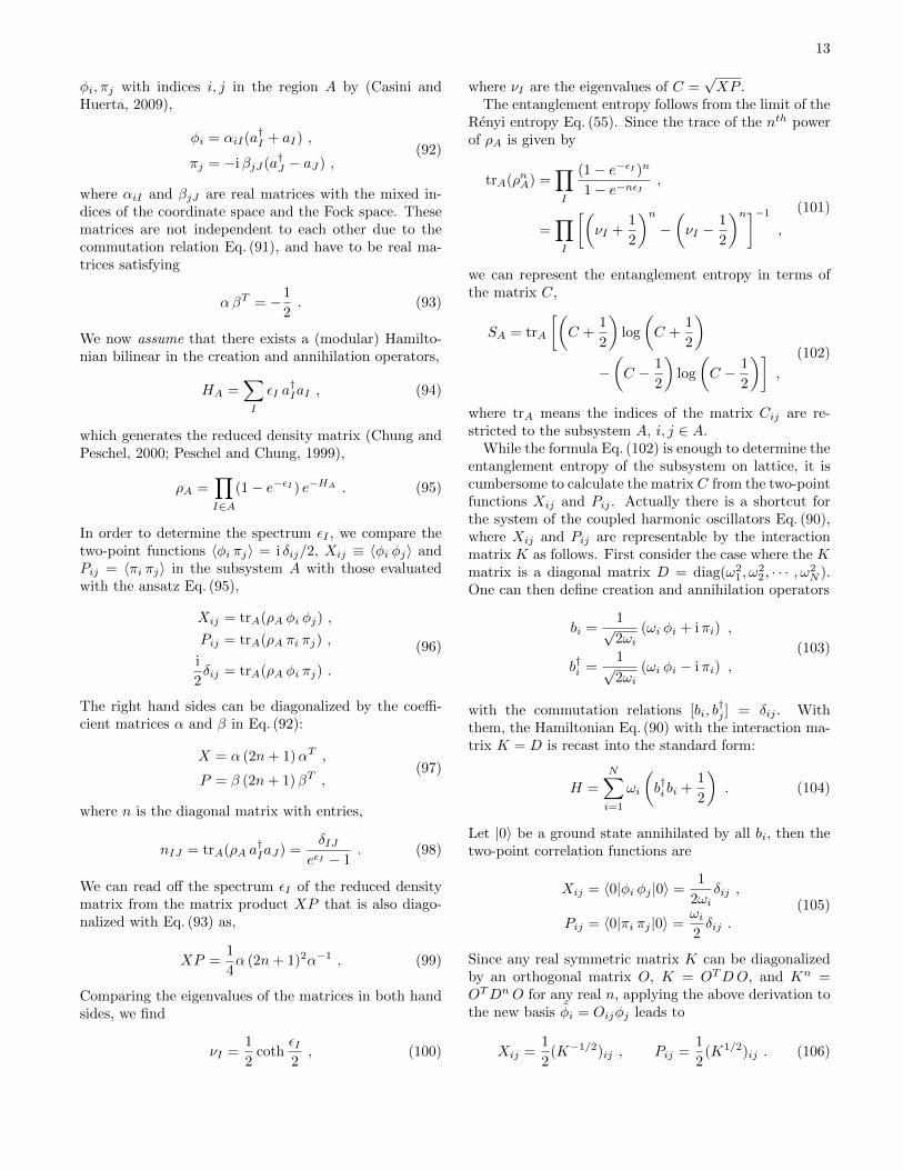
We assume the reader has background knowledgeabout the basics of QFT and general relativity. Somefamiliarity with conformal field theory in higher dimen-sions and QFT on a curved spacetime, covered by thestandard textbooks (Di Francesco et al., 1997) and (Bir-rell and Davies, 1982), would be also helpful.

The reader may refer to the other sources of literaturelisted below for more comprehensive treatments of thesubjects that we will or will not touch on in this article.

An introductory account of quantum entanglementin finite-dimensional systems is given in the textbook(Nielsen and Chuang, 2010) and the lecture notes(Preskill, 1997) with the emphasis on the application toquantum information theory. The implementation of the

real time approach is described for free lattice modelsin (Peschel and Eisler, 2009) and for free field theoriesin (Casini and Huerta, 2009) that also compares the ap-proach with the Euclidean formalism. The UV divergentstructures of entanglement entropy is discussed for lat-tice models in (Eisert et al., 2010) and for QFT on acurved space by employing the heat kernel method in(Solodukhin, 2011). The condensed matter applicationsof entanglement being a probe of quantum critical phe-nomena and quantum quench dynamics is elaborated inthe reviews (Calabrese and Cardy, 2009, 2016) by meansof the CFT methods (see also (Laflorencie, 2016)). Thedevelopments of the holographic method in the early daysare summarized in (Nishioka et al., 2009) and more re-cent ones in (Takayanagi, 2012). The role of quantumentanglement in the black hole information problem isemphasized in (Harlow, 2016). Recent attempts to buildup spacetime geometry from the entanglement structurein QFT can be found in (Van Raamsdonk, 2017). Theexact results for the F -theorem in supersymmetric fieldtheories are presented in (Pufu, 2016). Finally, we rec-ommend the reader to the textbook (Rangamani andTakayanagi, 2017) for a comprehensive overview of thewhole subjects.

II. ENTANGLEMENT IN QUANTUM MECHANICALSYSTEM

We shall introduce the notion of bipartite entangle-ment for pure states in finite-dimensional quantum me-chanical systems and classify the states into two typesdepending on whether they contain non-trivial entangle-ment entropy that quantifies the amount of quantum en-tanglement. A set of inequalities of entanglement en-tropy, which will play crucial roles in the latter sections,will be given without proofs. Other entanglement mea-sures frequently used in literature will also be introducedand compared with entanglement entropy.

A. Bipartite entanglement

Given a lattice model or QFT, suppose the system isin a pure ground state |Ψ〉, i.e., the density matrix forthe Hilbert space Htot is given in the form,2

ρtot = |Ψ〉〈Ψ| . (1)

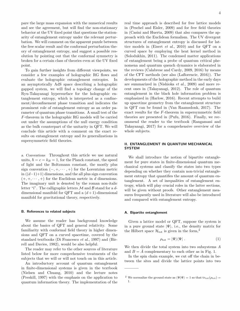
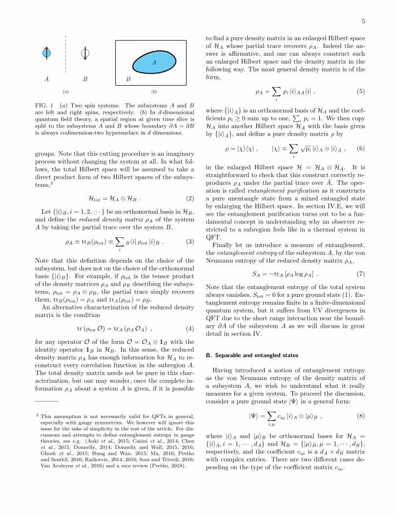
We then divide the total system into two subsystems Aand B = A complementary to each other as in Fig. 1.

In the spin chain example, we cut off the chain in be-tween the sites and divide the lattice points into two

2 We normalize the ground state as 〈Ψ|Ψ〉 = 1 so that trtot(ρtot) =1.

5

A B

(a)

A

B

(b)

FIG. 1 (a) Two spin systems. The subsystems A and Bare left and right spins, respectively. (b) In d-dimensionalquantum field theory, a spatial region at given time slice issplit to the subsystems A and B whose boundary ∂A = ∂Bis always codimension-two hypersurface in d dimensions.

groups. Note that this cutting procedure is an imaginaryprocess without changing the system at all. In what fol-lows, the total Hilbert space will be assumed to take adirect product form of two Hilbert spaces of the subsys-tems,3

Htot = HA ⊗HB . (2)

Let |i〉B , i = 1, 2, · · · be an orthonormal basis in HB ,and define the reduced density matrix ρA of the systemA by taking the partial trace over the system B,

ρA ≡ trB(ρtot) ≡∑i

B〈i| ρtot |i〉B . (3)

Note that this definition depends on the choice of thesubsystem, but does not on the choice of the orthonormalbasis |i〉B. For example, if ρtot is the tensor productof the density matrices ρA and ρB describing the subsys-tems, ρtot = ρA ⊗ ρB , the partial trace simply recoversthem, trB(ρtot) = ρA and trA(ρtot) = ρB .

An alternative characterization of the reduced densitymatrix is the condition

tr (ρtotO) = trA (ρAOA) , (4)

for any operator O of the form O = OA ⊗ 1B with theidentity operator 1B in HB . In this sense, the reduceddensity matrix ρA has enough information for HA to re-construct every correlation function in the subregion A.The total density matrix needs not be pure in this char-acterization, but one may wonder, once the complete in-formation ρA about a system A is given, if it is possible

3 This assumption is not necessarily valid for QFTs in general,especially with gauge symmetries. We however will ignore thisissue for the sake of simplicity in the rest of the article. For dis-cussions and attempts to define entanglement entropy in gaugetheories, see e.g. (Aoki et al., 2015; Casini et al., 2014; Chenet al., 2015; Donnelly, 2014; Donnelly and Wall, 2015, 2016;Ghosh et al., 2015; Hung and Wan, 2015; Ma, 2016; Pretkoand Senthil, 2016; Radicevic, 2014, 2016; Soni and Trivedi, 2016;Van Acoleyen et al., 2016) and a nice review (Pretko, 2018).

to find a pure density matrix in an enlarged Hilbert spaceof HA whose partial trace recovers ρA. Indeed the an-swer is affirmative, and one can always construct suchan enlarged Hilbert space and the density matrix in thefollowing way. The most general density matrix is of theform,

ρA =∑i

pi |i〉AA〈i| , (5)

where |i〉A is an orthonormal basis of HA and the coef-ficients pi ≥ 0 sum up to one,

∑i pi = 1. We then copy

HA into another Hilbert space HA with the basis givenby |i〉A, and define a pure density matrix ρ by

ρ = |χ〉〈χ| , |χ〉 ≡∑i

√pi |i〉A ⊗ |i〉A , (6)

in the enlarged Hilbert space H = HA ⊗ HA. It isstraightforward to check that this construct correctly re-produces ρA under the partial trace over A. The oper-ation is called entanglement purification as it constructsa pure unentangle state from a mixed entangled stateby enlarging the Hilbert space. In section IV.E, we willsee the entanglement purification turns out to be a fun-damental concept in understanding why an observer re-stricted to a subregion feels like in a thermal system inQFT.

Finally let us introduce a measure of entanglement,the entanglement entropy of the subsystem A, by the vonNeumann entropy of the reduced density matrix ρA,

SA = −trA [ρA log ρA] . (7)

Note that the entanglement entropy of the total systemalways vanishes, Stot = 0 for a pure ground state (1). En-tanglement entropy remains finite in a finite-dimensionalquantum system, but it suffers from UV divergences inQFT due to the short range interaction near the bound-ary ∂A of the subsystem A as we will discuss in greatdetail in section IV.

B. Separable and entangled states

Having introduced a notion of entanglement entropyas the von Neumann entropy of the density matrix ofa subsystem A, we wish to understand what it reallymeasures for a given system. To proceed the discussion,consider a pure ground state |Ψ〉 in a general form:

|Ψ〉 =∑i,µ

ciµ |i〉A ⊗ |µ〉B , (8)

where |i〉A and |µ〉B be orthonormal bases for HA =|i〉A, i = 1, · · · , dA and HB = |µ〉B , µ = 1, · · · , dB,respectively, and the coefficient ciµ is a dA × dB matrixwith complex entries. There are two different cases de-pending on the type of the coefficient matrix ciµ.

6

1. Separable state

When cij factorizes, cij = cAi cBµ , the ground state |Ψ〉

is called a separable state (a pure product states) and canbe recast into the product form,

|Ψ〉 = |ΨA〉 ⊗ |ΨB〉 , (9)

where |ΨA〉 ≡∑i cAi |i〉A and |ΨB〉 ≡

∑µ c

Bµ |µ〉B . This is

the case where the reduced density matrix, Eq. (3), alsobecomes pure, ρA = |ΨA〉〈ΨA|. Thus a separable statehas vanishing entanglement entropy,

SA = 0 . (10)

Moreover, one can show entanglement entropy vanishesif and only if the pure ground state is separable as wewill see in a moment below.

2. Entangled state

The ground state is called an entangled (or inseparable)state if it is not separable (with the coefficient matrixciµ 6= cAi c

Bµ ). This is the case where the entanglement

entropy takes a positive value.

Indeed, we can simplify the form Eq. (8) by changingthe bases into the Schmidt decomposition form,

|Ψ〉 =

min(dA,dB)∑k=1

√pk |ψk〉A ⊗ |ψk〉B , (11)

where pk are non-negative real numbers satisfying∑k pk = 1 and |ψk〉A,B are new orthonormal bases for

the subsystems A and B. Note that this decompositionworks for any dA×dB rectangular matrix ciµ. To see howit actually works, we “diagonalize” the coefficient matrixby the singular-value decomposition,

c = U ΣV † , (12)

where U, V are dA × dA and dB × dB unitary matrices.Σ is a diagonal dA × dB real matrix given by

Σ =

√p1

. . . 0√pdB

, (dA < dB) ,

√p1

. . .√pdA

0

, (dA ≥ dB) ,

(13)

with non-negative real entries√pk ≥ 0, k =

1, · · · ,min(dA, dB). The square root for the eigenval-ues is purely conventional for later use. The new or-thonormal bases |ψk〉A,B are the unitary transformationof the original ones |i〉A,B as |ψk〉A =

∑i Uik|i〉A and

|ψk〉B =∑µ Vkµ|µ〉B .

The Schmidt decomposition Eq. (11) is particularlynice as it yields a mixed state density matrix with theprobability distribution pk for the reduced density ma-trix,

ρA =

dB∑i=1

B〈ψi|Ψ〉〈Ψ|ψi〉B ,

=

min(dA,dB)∑k=1

pk |ψk〉A A〈ψk| .

(14)

In our case, the condition∑k pk = 1 follows from the

normalization 〈Ψ|Ψ〉 = 1. We see that the reduced den-sity matrix of a subsystem can be mixed even if the to-tal system is in a pure ground state. This should becompared with the discussion for entanglement purifica-tion around Eq. (6) where we saw the opposite. In theSchmidt decomposition the entanglement entropy

SA = −min(dA,dB)∑

k=1

pk log pk , (15)

is nothing but the Shannon entropy of the probabilitydistribution pk. Under the constraint

∑k pk = 1, it

takes the maximum value

SA|max = log min(dA, dB) , (16)

at pk = 1/min(dA, dB) for any k.4

In summary, an entangled state is a superposition ofseveral quantum states. An observer who can only accessto a subsystem A will find him or herself in a mixed statewhen the pure ground state |Ψ〉 in the total system isentangled:

|Ψ〉 : separable ←→ ρA : pure state ,

|Ψ〉 : entangled ←→ ρA : mixed state .(17)

Entanglement entropy measures how much a givenstate differs from a separable state. It reaches to themaximum value when a given state is a superposition ofall possible quantum states with an equal weight.

4 To prove Eq. (16), one may introduce the Lagrange multiplierx (

∑k pk − 1) to the entropy Eq. (15) and extremize it with re-

spect to pk.

7

a. Two spin system Let us illustrate a simple example ofan entangled state. Consider a system of two particlesA and B with spin 1/2. The Hilbert spaces HA and HBare spanned by two states: HA,B = |0〉A,B , |1〉A,B. Welet them be orthonormal bases satisfying A,B〈i|j〉A,B =δij for i, j = 0, 1. Since the total Hilbert space is thetensor product of the two subsystems Htot = HA ⊗HB ,it has the four-dimensional orthonormal basis: Htot =|00〉, |01〉, |10〉, |11〉 where |ij〉 ≡ |i〉A ⊗ |j〉B are tensorproduct states.

Suppose the ground state is given by

|Ψ〉 =1√2

(|01〉 − |10〉

). (18)

The reduced density matrix for the particle A is obtainedby taking the partial trace over HB of the total densitymatrix Eq. (1),

ρA =1

2

(|0〉A A〈0|+ |1〉A A〈1|

). (19)

It is neat to write it in a matrix form acting on the two-dimensional vector space HA,

ρA =

(1/2 00 1/2

). (20)

It clearly shows that ρA is not pure and the entanglemententropy does not vanish,

SA = −trA

[(1/2 00 1/2

)(log(1/2) 0

0 log(1/2)

)],

= log 2 .

(21)

This is a maximally entangled state for it saturates theupper bound Eq. (16) with dA = dB = 2.

A more general state to consider is

|Ψ〉 = cos θ |01〉 − sin θ |10〉 , (22)

parametrized by a parameter θ ranging from 0 to π2 , that

reduces the state Eq. (18) at θ = π/4. By a similar cal-culation we have

SA = − cos2 θ log(cos2 θ)− sin2 θ log(sin2 θ) , (23)

which shows the states at θ = 0, π/2 are pure prod-uct states with vanishing entanglement entropy while thestate Eq. (18) at θ = π/4 is maximally entangled.

b. Thermofield double state A more non-trivial exampleof an entangled state is the thermofield double state de-fined by

|Ψ〉 =1√Z

∑n

e−βEn/2|n〉A ⊗ |n〉B , (24)

where we normalize the state with the partition func-tion Z =

∑n e−βEn . The peculiarity of the thermofield

double state becomes manifest in taking the partial traceover the subsystem B. Namely the reduced density ma-trix for the subsystem A becomes a Gibbs state of inversetemperature β:

ρA =1

Z

∑n

e−βEn |n〉AA〈n| ,

=1

Ze−βHA .

(25)

In the second line, we introduced the (modular) Hamilto-nian HA such that HA|n〉A = En|n〉A. Actually the ther-mofield double state is the entanglement purification of athermal state with the Boltzmann weight pi = e−β Ei/Zin Eq. (6). Namely we can purify the thermal system A inthe extended Hilbert spaceHA⊗HB by copying the statevectors |n〉B from HA to HB . Then every expectationvalue of local operators in the thermal system A is rep-resentable in the thermofield double state Eq. (24) of thetotal system A ∪ B. In this example, the entanglemententropy measures the thermal entropy of the subsystemA:

SA = −trA [ρA (−βHA − logZ)] ,

= β (〈HA〉 − F ) ,(26)

where F is the thermal free energy β F = − logZ.The thermofield double state is also important to un-

derstand the thermal nature of black holes when we con-sider QFT on a background geometry with a horizon insection IV.E.

C. Bell states

In the two spin system, we saw the state Eq. (18) ismaximally entangled. Actually there are totally four in-dependent maximally entangled states in the two qubitsystem:

|B1〉 =1√2

(|00〉+ |11〉

),

|B2〉 =1√2

(|00〉 − |11〉

),

|B3〉 =1√2

(|01〉+ |10〉

),

|B4〉 =1√2

(|01〉 − |10〉

).

(27)

These are known as the Bell states or Einstein-Podolsky-Rosen (EPR) pairs in quantum information theory.These states manifest their quantum mechanical aspectsin a sense that they violate the Bell’s inequalities hold-ing in a local hidden variable theory accounting for theprobabilistic features of quantum mechanics with a hid-den variable and a probability density.

8

For a system of n qubits, there are entangle statescalled the Greenberger-Horne-Zeilinger (GHZ) states(Greenberger et al., 1990, 1989):

|GHZ〉 =1√2

(|0〉⊗n + |1〉⊗n

). (28)

Another type of entangled states is called the W state(Dur et al., 2000),

|W 〉 =1√n

(|10 · · · 00〉+ |010 · · · 0〉+ · · ·+ |00 · · · 01〉) .

(29)

These two types of states are inequivalent as the GHZstate is fully separable while the W state is not as seenbelow.

a. Tripartite system In a tripartite system (n = 3), theGHZ and W states become

|GHZ〉 =1√2

(|000〉+ |111〉) , (30)

and

|W 〉 =1√3

(|001〉+ |010〉+ |100〉) . (31)

We denote the three subsystems by A,B and C. Tracingout the Hilbert space of the subsystem C, the reduceddensity matrices for the system A ∪B are

ρ(GHZ)A∪B =

1

2(|00〉〈00|+ |11〉〈11|) ,

ρ(W)A∪B =

2

3|B3〉〈B3|+

1

3|00〉〈00| .

(32)

The ρ(GHZ)A∪B is fully separable in a sense that it can be

written in the form

ρ(GHZ)A∪B =

k∑i=1

pi ρ(i)A ⊗ ρ

(i)B , (33)

where k = 2, pi = 1/2 and ρ(1)A,B = |0〉〈0|, ρ(2)

A,B = |1〉〈1|.On the other hand, the ρ

(W)A∪B cannot be written in such

a form because of the appearance of the Bell state |B3〉.This implies that the W state is still entangled even afterthe partial trace.

D. Properties of entanglement entropy

Entanglement entropy enjoys several useful propertiesthat we will summarize without proofs below. An inter-ested reader may refer to (Nielsen and Chuang, 2010) forthe derivations and the other properties.

• If a ground state wave function is pure, the entan-glement entropy of the subsystem A and its com-plement B = A are the same:

SA = SB . (34)

This follows from the symmetry of the Schmidt de-composition under the exchange of A and B andalso from the result Eq. (15). However, SA is nolonger equal to SB when the total system is in amixed state e.g., at finite temperature.

• Given two disjoint subsystems A and B, the entan-glement entropies satisfy the subadditivity,

SA∪B ≤ SA + SB , (35)

Also it satisfies the triangle inequality or the Araki-Lieb inequality (Araki and Lieb, 1970),

|SA − SB | ≤ SA∪B , (36)

which is symmetric between A and B.

• For any three disjoint subsystems A, B and C, thefollowing inequalities hold:

SA∪B∪C + SB ≤ SA∪B + SB∪C ,

SA + SC ≤ SA∪B + SB∪C ,(37)

These are known as the strong subadditivity, themost fundamental inequalities for entanglemententropy. The two inequalities are shown to beequivalent to each other (Araki and Lieb, 1970).The proof is based on a convexity of a functionbuild from the density matrix that is Hermitianwhen a system is unitary (Lieb and Ruskai, 1973;Narnhofer and Thirring, 1985). The subadditivityEq. (35) and the Araki-Lieb inequality Eq. (36) arederivable from the strong subadditivity.

The strong subadditivity of entanglement will play vi-tal roles in the entropic proofs of the c- and F -theoremsfor renormalization group flows in QFT as we will see insection VIII.

E. Relations between entanglement measures

Among several measures of quantum entanglement welist a few, relative entropy, mutual information and Renyientropy, that are often used in the applications to QFT,and discuss their features and connections to each other.

1. Relative entropy

Given two states described by the density matrices ρ, σ,one can define the relative entropy by (Umegaki et al.,1962)

S(ρ||σ) = tr [ρ (log ρ− log σ)] . (38)

9

It measures the “distance” between the two states withseveral (defining) properties (Ohya, 2004; Vedral, 2002),

S(ρ||ρ) = 0 , (39)

S(ρ1 ⊗ ρ2||σ1 ⊗ σ2) = S(ρ1||σ1) + S(ρ2||σ2) , (40)

S(ρ||σ) ≥ 1

2||ρ− σ||2 , (41)

S(ρ|σ) ≥ S(trp ρ|trp σ) , (42)

where the trp is a partial trace with respect to the sub-system p, and the norm means

||ρ|| = tr (√ρ†ρ) . (43)

With particular choices of the density matrices, the rel-ative entropy reduces to entanglement entropy,

S(ρA||1A/dA) = log dA − SA , (44)

where 1A is the dA × dA unit matrix for the dA-dimensional Hilbert space of the region A.

The relative entropy is always non-negative, S(ρ||σ) ≥0, bounded from below by the inequality Eq. (41). Vari-ous inequalities for the other entanglement measures fol-low from the monotonicity of the relative entropy givenby Eq.(42) (see Table I). For example, the strong subad-ditivity Eq. (37) is derivable as follows.

Let ρA∪B∪C be the density matrix for the total sys-tem A ∪ B ∪ C, and we denote its restrictions to thesubsystems A ∪B,B ∪C and B by ρA∪B , ρB∪C and ρB ,respectively. Since the reduced density matrices have theproperty such that trA∪B∪C [ρA∪B∪C (OA∪B⊗1C/dC)] =trA∪B(ρA∪B OA∪B), we can show the identities,

S(ρA∪B∪C ||1A∪B∪C/dA∪B∪C)

= S(ρA∪B ||1A∪B/dA∪B) + S(ρA∪B∪C ||ρA∪B ⊗ 1C/dC) ,

S(ρB∪C ||1B∪C/dB∪C)

= S(ρB ||1B/dB) + S(ρB∪C ||ρB ⊗ 1C/dC) .

(45)

On the other hand, the monotonicity Eq. (42) implies

S(ρA∪B∪C ||ρA∪B ⊗ 1C/dC) ≥ S(ρB∪C ||ρB ⊗ 1C/dC) ,(46)

and combined with the equalities Eq. (45), we arrive atthe inequality,

S(ρA∪B∪C ||1A∪B∪C/dA∪B∪C) + S(ρB ||1B/dB)

≥ S(ρA∪B ||1A∪B/dA∪B) + S(ρB∪C ||1B∪C/dB∪C) .

(47)

Translating the relative entropy to entanglement entropythrough Eq. (44) and noting the dimensional relationslike dA∪B∪C = dAdBdC , we find Eq. (47) is nothing butthe strong subadditivity of entanglement entropy givenby the first line of Eq. (37). We do not bother to derive

TABLE I Equivalence between the entanglement inequalitiesof various measures

Entanglement entropy Mutual information Relative entropySubadditivity Positivity Positivity

Eq. (35) Eq. (50) Eq. (41)

Strong subadditivity Monotonicity MonotonicityEq. (37) Eq. (51) Eq. (42)

the second inequality in Eq. (37) from the monotonicity ofthe relative entropy as it is equivalent to the first (Arakiand Lieb, 1970).

One can estimate a lower bound for the relative en-tropy by combining Eq. (41) with the Schwarz inequality||X|| ≥ tr(XY )/||Y ||,

S(ρ||σ) ≥ 1

2

(〈O〉ρ − 〈O〉σ)2

||O||2, (48)

where 〈O〉ρ is the expectation value of an operator Owith the density matrix ρ.

2. Mutual information

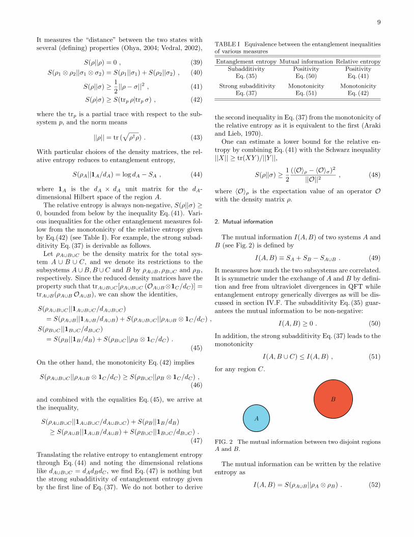
The mutual information I(A,B) of two systems A andB (see Fig. 2) is defined by

I(A,B) ≡ SA + SB − SA∪B . (49)

It measures how much the two subsystems are correlated.It is symmetric under the exchange of A and B by defini-tion and free from ultraviolet divergences in QFT whileentanglement entropy generically diverges as will be dis-cussed in section IV.F. The subadditivity Eq. (35) guar-antees the mutual information to be non-negative:

I(A,B) ≥ 0 . (50)

In addition, the strong subadditivity Eq. (37) leads to themonotonicity

I(A,B ∪ C) ≤ I(A,B) , (51)

for any region C.

A

B

FIG. 2 The mutual information between two disjoint regionsA and B.

The mutual information can be written by the relativeentropy as

I(A,B) = S(ρA∪B ||ρA ⊗ ρB) . (52)

10

This relation shows that the mutual information betweentwo subsystems quantifies how much the state ρA∪B forthe union A∪B differs from the separable state ρA⊗ ρBand can be a good measure of global correlations overspatially disconnected regions in QFT.

Combining the third inequality of Eq. (41) and theexpression of the mutual information Eq. (52) with theSchwarz inequality, one obtains the lower bound for themutual information (Wolf et al., 2008),

I(A,B) ≥ 1

2

(〈OAOB〉 − 〈OA〉〈OB〉)2

||OA||2||OB ||2, (53)

where OA and OB are any bounded operators in the re-gions A and B, respectively.

3. Renyi entropy

The Renyi entropy is a one-parameter generalizationof entanglement entropy labeled by an integer n, calledthe replica parameter (Renyi, 1961),

Sn(A) =1

1− nlog trA(ρnA) . (54)

In the n → 1 limit with the normalization trA(ρA) = 1,the Renyi entropy reduced to entanglement entropy,

SA = limn→1

Sn(A) . (55)

The Renyi entropy provides us more information aboutthe eigenvalues of the reduced density matrix than entan-glement entropy. It is defined for an integer n, but oneassume an analytic continuation of n to a real number intaking the limit Eq. (55). This analytic continuation willbe useful to compute entanglement entropy of QFT bythe replica method in section IV.

a. Thermal interpretation of Renyi entropic inequalities

The Renyi entropy Eq. (54) is shown to satisfy severalinequalities between different values of n (Zyczkowski,2003),

∂nSn ≤ 0 , (56)

∂n

(n− 1

nSn

)≥ 0 , (57)

∂n ((n− 1)Sn) ≥ 0 , (58)

∂2n ((n− 1)Sn) ≤ 0 . (59)

To grasp the physical meaning of these inequalities weintroduce the modular Hamiltonian HA by

ρA ≡ e−2πHA , (60)

and consider a “thermal” partition function

Z(β) ≡ trA(ρnA) = trA(e−βHA) , (61)

at inverse temperature β ≡ 2πn when HA regarded asa Hamiltonian. In analogy to statistical mechanics wecan define the modular energy E(β), the modular entropyS(β), and the modular capacity C(β)5 by the canonicalrelations,

E(β) ≡ −∂β logZ(β) ,

S(β) ≡ (1− β∂β) logZ(β) ,

C(β) ≡ β2∂2β logZ(β) .

(62)

With these “thermodynamic” quantities, the inequalitiesEq. (57), Eq. (58) and Eq. (59) are rewritten in more con-cise forms (Hung et al., 2011b; Nakaguchi and Nishioka,2016):

S(β) ≥ 0 ,

E(β) ≥ 0 ,

C(β) ≥ 0 .

(63)

The inequality Eq. (56) is not independent from the oth-ers and can be derived from Eq. (59). We thus find theinequalities of Renyi entropy have a nice interpretationas the stability of the thermal system when the replicaparameter n is regarded as the inverse temperature forthe modular Hamiltonian.

There is a one-to-one correspondence between themodular entropy and the Renyi entropy,

Sn ≡ n2∂n

(n− 1

nSn

), (64)

where we changed the notation for S(β) to emphasizethe n dependence. Inverting this relation by integration,we can reconstruct the Renyi entropy from the modularentropy,

Sn =n

n− 1

∫ n

1

dn1

n2Sn . (65)

We will discuss the implications of the inequalitiesEq. (63) for a gravitational system when a holographicdescription of the Renyi entropy is available in sectionVII.E.

b. Relative Renyi entropy The relative Renyi entropy isan analogue of the Renyi entropy for the relative entropy,defined by (Muller-Lennert et al., 2013; Wilde et al.,2013)

Sn(ρ||σ) =1

n− 1log[tr(σ(1−n)/(2n)ρ σ(1−n)/(2n))n

],

(66)

5 The modular capacity C(β) is the same as the capacity of entan-glement defined by Yao and Qi (2010).

11

for n ∈ (0, 1) ∪ (1,∞) and

S1(ρ||σ) = S(ρ||σ) ,

S∞(ρ||σ) = log ||σ−1/2ρ σ−1/2||∞ .(67)

The relative Renyi entropy is shown to be monotonicunder the partial trace operation trp,

Sn(ρ||σ) ≥ Sn(trp ρ||trp σ) , (68)

for n ≥ 1/2 as is the relative entropy (Beigi, 2013; Frankand Lieb, 2013).

The relative Renyi entropy reduces to the Renyi en-tropy in taking a special state as σ in the same way asin Eq. (44),

Sn(ρA||1A/dA) = log dA − Sn(A) , (69)

It is also shown to be monotonic with respect the param-eter n (Beigi, 2013; Muller-Lennert et al., 2013),

∂nSn(ρ||σ) ≥ 0 , (70)

which is considered as a generalization of the inequalityEq. (56) for the Renyi entropy.

One may be tempted to define the Renyi mutual in-formation in a similar manner to the mutual informationEq. (49). This naive construction, however, can give riseto a negative value for a certain class of states when n 6= 1in general, and does not allow the interpretation as anentanglement measure of quantum information (Adessoet al., 2012).6

Instead, one can introduce the n-Renyi mutual infor-mation by (Beigi, 2013)

In(A,B) = minσBSn(ρA∪B ||ρA ⊗ σB) , (72)

where the minimum is taken over all density matrices σB .It is always non-negative by definition and reduces to themutual information when n = 1.

F. Entanglement entropy at finite temperature

The entanglement entropy SA(T ) at finite temperatureT = β−1 can be defined just by replacing the total densitymatrix Eq. (1) with the thermal density matrix

ρthermal =e−βH

tr(e−βH), (73)

6 An example of such states for n = 2 is

ρA∪B = x |00〉〈00|+ y |01〉〈01|+ (1− x− y) |10〉〈10| , (71)

with the parameter ranges 0 < x < 1/2 and 0 < y < (1/2 −x)/(1− x).

where H is the Hamiltonian of the total system. Bydefinition, SA(β) equals the thermal entropy when A isthe total system

Stot = Sthermal . (74)

Let |Ψ〉 be the ground state with no energy H|Ψ〉 = 0,and |φ〉 be the first excited (normalized) state with theenergy H|φ〉 = Eφ|φ〉. Then the density matrix has anexpansion around the ground state at zero temperature,

ρthermal =|Ψ〉〈Ψ|+ |φ〉〈φ| e−βEφ + · · ·

1 + e−βRφ + · · ·, (75)

The reduced density matrix allows a similar expansion,

ρA = ρ0A + e−βEφ (ρφA − ρ0A) + · · · , (76)

where we defined ρ0A ≡ trB(|Ψ〉〈Ψ|) and ρφA ≡trB(|φ〉〈φ|). It follows from the n→ 1 limit of the Renyientropy Eq. (54) that the entanglement entropy receivesthe universal thermal contribution from the excited state(Cardy and Herzog, 2014; Herzog, 2014),

SA(T ) = SA(T = 0) + e−βEφ∆〈H0A〉+ · · · , (77)

where H0A ≡ − log ρ0A is the modular Hamiltonian forthe ground state and ∆〈H0A〉 stands for the difference ofthe modular Hamiltonian,

∆〈H0A〉 ≡ trA [H0A(ρφA − ρ0A)] . (78)

III. REAL TIME FORMALISM

We will illustrate the real time approach for calculat-ing the reduced density matrix of a subsystem in theHamiltonian description. This method is suitable for thenumerical computation once we discretize the spacetimeto lattice. We will describe only the bosonic case hereand defer the fermionic case to appendix A.

A. Two coupled harmonic oscillators

To illustrate the real time approach, we start witha simple example of two coupled harmonic oscillators(Bombelli et al., 1986; Srednicki, 1993) (see Fig. 3). Sup-pose this system is described by the Hamiltonian,

H =1

2

[p2A + p2

B + k(x2A + x2

B) + l(xA − xB)2], (79)

where xA,B and pA,B are the positions and the conju-gate momenta of the two oscillators, and k, l are re-lated to their mass and the coupling. First of all, wewant to find the ground state wave function of the sys-tem. To this end, we introduce new variables x± =(xA ± xB)/

√2, ω+ = k1/2 and ω− = (k + 2l)1/2. In

12

these new variables, the Hamiltonian is for two uncou-pled harmonic oscillators and the Schrodinger equationbecomes

1

2

[−∂2

+ − ∂2− + ω2

+x2+ + ω2

−x2−]

Ψ(x+, x−) = EΨ(x+, x−) .

(80)

Then the ground state wave function is the product oftwo copies of the ground state wave function of one har-monic oscillator,

Ψ(x+, x−) =(ω+ω−)1/4

π1/2exp

[−ω+x

2+ + ω−x

2−

2

], (81)

with the energy E = (ω+ + ω−)/2. The overall factoris chosen so that the wave function is normalized to be∫∞−∞ dxA

∫∞−∞ dxB |Ψ(xA, xB)|2 = 1 where we denote the

wave function in the original variables xA and xB by thesame symbol Ψ(xA, xB).

Next, we trace out the oscillator at xB and con-struct the reduced density matrix ρA for the oscillatorat xA. If we represent the ground state wave function asΨ(xA, xB) = (〈xA| ⊗ 〈xB |)|Ψ〉, then the reduced densitymatrix follows as

ρA(xA, x′A) = 〈xA|trB (|Ψ〉〈Ψ|) |x′A〉 ,

=

∫ ∞−∞

dxB Ψ(xA, xB) Ψ∗(x′A, xB) ,

=

√γ − βπ

exp[−γ

2(x2A + x′2A) + β xAx

′A

],

(82)

where we introduced the parameters

β =(ω+ − ω−)2

4(ω+ + ω−), γ =

2ω+ω−ω+ + ω−

+ β . (83)

Finally, we need the eigenvalues of the reduced den-sity matrix to compute the entanglement entropy. Theeigenfunction fn with the eigenvalue pn must satisfy∫ ∞

−∞dx′ ρA(x, x′) fn(x′) = pn fn(x) , (84)

and the solution is given by

fn(x) = Hn(α1/2x) e−αx2

2 , (n = 0, 1, 2, · · · ) ,(85)

where α = (ω+ω−)1/2 and Hn is the Hermite polynomial.The eigenvalue pn is

pn = (1− ξ) ξn , ξ =β

α+ γ. (86)

One way to derive the eigenfunction is to expand thereduced density matrix by the Hermite polynomial,

ρA(x, x′) =

√α

π(1− ξ) e−α2 (x2+x′2)

·∞∑n=0

ξn

2nn!Hn(α1/2x)Hn(α1/2x′) ,

(87)

and use the orthogonality,∫ ∞−∞

dx e−x2

Hn(x)Hm(x) =√π 2nn! δnm . (88)

Having diagonalized the reduced density matrix, we areready to obtain the entanglement entropy from the eigen-value Eq. (86),

SA = −∞∑n=0

pn log pn ,

= − log(1− ξ)− ξ

1− ξlog ξ .

(89)

B. N-coupled harmonic oscillators

It is straightforward to generalize the model Eq. (79) oftwo harmonic oscillators to a system of N -coupled har-monic oscillators (see Fig. 3)

H =1

2

N∑i=1

π2i +

1

2

N∑i,j=1

φiKij φj , (90)

where K is a real symmetric matrix and πi is a canonicalconjugate momentum of the oscillator φi satisfying thecommutation relation,7

[φi, πj ] = i δij . (91)

It reduces to the previous model Eq. (79) for N = 2,K11 = K22 = k + l and K12 = −l. Instead of repeatingthe arguments in literatures (Bombelli et al., 1986; Sred-nicki, 1993), we adopt a different method that suites fornumerical computation.

A B

FIG. 3 A system of N -coupled harmonic oscillators. Herethe total size of the system is N = 10 and the subsystem Aconsists of four oscillators from the left.

First, we introduce creation and annihilation operatorsaI , a

†I satisfying the commutation relation, [aI , a

†J ] = δIJ .

Note that the new indices I, J are different from the in-dices i, j labeling the lattice site. They parametrize theFock space generated by aI and a†I . We assume the oper-

ators aI , a†I are linearly related to the original oscillators

7 The oscillator and conjugate momentum are considered as her-mitian operators.

13

φi, πj with indices i, j in the region A by (Casini andHuerta, 2009),

φi = αiI(a†I + aI) ,

πj = −iβjJ(a†J − aJ) ,(92)

where αiI and βjJ are real matrices with the mixed in-dices of the coordinate space and the Fock space. Thesematrices are not independent to each other due to thecommutation relation Eq. (91), and have to be real ma-trices satisfying

αβT = −1

2. (93)

We now assume that there exists a (modular) Hamilto-nian bilinear in the creation and annihilation operators,

HA =∑I

εI a†IaI , (94)

which generates the reduced density matrix (Chung andPeschel, 2000; Peschel and Chung, 1999),

ρA =∏I∈A

(1− e−εI ) e−HA . (95)

In order to determine the spectrum εI , we compare thetwo-point functions 〈φi πj〉 = i δij/2, Xij ≡ 〈φi φj〉 andPij = 〈πi πj〉 in the subsystem A with those evaluatedwith the ansatz Eq. (95),

Xij = trA(ρA φi φj) ,

Pij = trA(ρA πi πj) ,

i

2δij = trA(ρA φi πj) .

(96)

The right hand sides can be diagonalized by the coeffi-cient matrices α and β in Eq. (92):

X = α (2n+ 1)αT ,

P = β (2n+ 1)βT ,(97)

where n is the diagonal matrix with entries,

nIJ = trA(ρA a†IaJ) =

δIJeεI − 1

. (98)

We can read off the spectrum εI of the reduced densitymatrix from the matrix product XP that is also diago-nalized with Eq. (93) as,

XP =1

4α (2n+ 1)2α−1 . (99)

Comparing the eigenvalues of the matrices in both handsides, we find

νI =1

2coth

εI2, (100)

where νI are the eigenvalues of C =√XP .

The entanglement entropy follows from the limit of theRenyi entropy Eq. (55). Since the trace of the nth powerof ρA is given by

trA(ρnA) =∏I

(1− e−εI )n

1− e−nεI,

=∏I

[(νI +

1

2

)n−(νI −

1

2

)n]−1

,

(101)

we can represent the entanglement entropy in terms ofthe matrix C,

SA = trA

[(C +

1

2

)log

(C +

1

2

)−(C − 1

2

)log

(C − 1

2

)],

(102)

where trA means the indices of the matrix Cij are re-stricted to the subsystem A, i, j ∈ A.

While the formula Eq. (102) is enough to determine theentanglement entropy of the subsystem on lattice, it iscumbersome to calculate the matrix C from the two-pointfunctions Xij and Pij . Actually there is a shortcut forthe system of the coupled harmonic oscillators Eq. (90),where Xij and Pij are representable by the interactionmatrix K as follows. First consider the case where the Kmatrix is a diagonal matrix D = diag(ω2

1 , ω22 , · · · , ω2

N ).One can then define creation and annihilation operators

bi =1√2ωi

(ωi φi + iπi) ,

b†i =1√2ωi

(ωi φi − iπi) ,

(103)

with the commutation relations [bi, b†j ] = δij . With

them, the Hamiltonian Eq. (90) with the interaction ma-trix K = D is recast into the standard form:

H =

N∑i=1

ωi

(b†i bi +

1

2

). (104)

Let |0〉 be a ground state annihilated by all bi, then thetwo-point correlation functions are

Xij = 〈0|φi φj |0〉 =1

2ωiδij ,

Pij = 〈0|πi πj |0〉 =ωi2δij .

(105)

Since any real symmetric matrix K can be diagonalizedby an orthogonal matrix O, K = OTDO, and Kn =OTDnO for any real n, applying the above derivation tothe new basis φi = Oijφj leads to

Xij =1

2(K−1/2)ij , Pij =

1

2(K1/2)ij . (106)

14

The matrix C =√XP is constant, C = 1/2, when

A is the total system, and the entanglement entropyEq. (102) clearly vanishes in this case as expected. Onthe other hand, it no longer vanishes for a subsystemA specified by i = 1, · · · , NA where NA < N becauseCij = (

∑k=1,··· ,NA(K−1/2)ik(K1/2)kj)

1/2/2 is not nec-essarily 1/2 in general.

C. Free massive scalar fields

The argument used in the previous subsection can beextended to higher-dimensional theories without diffi-culty if the system has rotational symmetry. Namely,for a spherical entangling surface, the system can be ef-fectively reduced to (1 + 1)-dimensional theories on theradial coordinate (Huerta, 2012; Lohmayer et al., 2010;Srednicki, 1993).

Consider a free massive real scalar field with the ac-tion8

I = −1

2

∫ddx√−g

[(∂µφ)2 +m2φ2

]. (107)

We put the theory on the radial coordinates,

ds2 = −dt2 + dr2 + r2dΩ2d−2 , (108)

where dΩ2d−2 is the metric for a unit (d − 2)-sphere.

Rescaling the scalar field φ by rd/2−1 and Fourier decom-posing along the angular directions simplifies the Hamil-tonian,

H =1

2

∞∑l=0

gs(d− 2, l)

·∫ ∞

0

dr

π2l (r) + rd−2

[∂r

(φl(r)

rd/2−1

)]2

+

(m2 +

l(l + d− 3)

r2

)φ2l (r)

,

(109)

where πl are the conjugate momenta of the field φl withthe orbital angular momentum l, satisfying the commu-tation relation

[φl(r), πl′(r′)] = i δll′δ(r − r′) . (110)

The factor gs(d, l) is the degeneracy of the lth angularmode of a scalar field on unit d-sphere Sd,

g(d, l) =(2l + d− 1)Γ(l + d− 1)

l! Γ(d). (111)

8 We may use a non-minimally coupled scalar field with a termRφ2 in the action, but the result is the same as the minimallycoupled case (Casini et al., 2015b; Herzog and Nishioka, 2016).

We discretize the radial coordinate r to N sitesparametrized by i with lattice spacing a, that leads tothe following replacement rule:

r → i a , δ(r − r′) → δii′

a,

φl(r) → φl,i , πl(r) →πl,ia

.(112)

for the terms without derivatives and

r →(i+

1

2

)a ,

∂r

(φl(r)

rd/2−1

)→ 1

ad/2

[φl,i+1

(i+ 1)d/2−1− φl,iid/2−1

],

(113)

for the terms with derivatives.9 The resulting Hamilto-nian on the lattice takes the similar form as Eq. (90) forthe N -coupled harmonic oscillator:

H =1

2a

∞∑l=0

gs(d− 2, l)

N∑i=1

π2l,j +

N∑i,j=1

φl,iKijl φl,j

.

(114)

The symmetric matrix Kl is chosen to be

K11l =

(3

2

)d−2

+ l(l + d− 3) + (ma)2 ,

Kiil =

1

id−2

[(i− 1

2

)d−2

+

(i+

1

2

)d−2]

+l(l + d− 3)

i2+ (ma)2 ,

Ki,i+1l = Ki+1,i

l = − (i+ 1/2)d−2

id/2−1(i+ 1)d/2−1.

(115)

Hence the entanglement entropy of a free massive scalarfield for a spherical system amounts to the summation ofthose over each angular mode,

SA =

∞∑l=0

gs(d− 2, l)Sl , (116)

where Sl is the entropy for the lth mode of the formEq. (102) ,

Sl = trA

[(Cl +

1

2

)log

(Cl +

1

2

)−(Cl −

1

2

)log

(Cl −

1

2

)],

(117)

9 Among several discretization schemes we exclusively use Sred-nicki lattice (Srednicki, 1993) in this article.

15

with Cl = (Cl)ij for i, j ∈ A being

(Cl)ij =1

2

[∑k∈A

(K−1/2l )ik(K

1/2l )kj

]1/2

. (118)

For a spherical entangling surface of radius R, the indicesi, j, k ∈ A range from 1 to NA where NA is fixed byR = (NA + 1/2)a.

IV. EUCLIDEAN FORMALISM

In this section, we will rewrite the definition of en-tanglement entropy by introducing an auxiliary (replica)parameter. After giving a representation of the reduceddensity matrix in terms of the path integral, we will de-rive an expression of the entanglement entropy given bythe Euclidean partition function on a singular manifold.This approach is sometimes easier than the real time ap-proach in performing analytic computations in QFT.

A. Replica trick

We adopt the definition Eq. (7) of entanglement en-tropy with Eq. (54) and Eq. (55),

SA = − limn→1

log trA(ρnA)

n− 1,

= − limn→1

∂n log trA(ρnA) ,(119)

where we used the fact that the reduced density matrix isnormalized, trA(ρA) = 1. Although the Renyi entropy isdefined only for an integer n, the analytic continuation isassumed in taking n→ 1 limit. This method is called thereplica trick that is often employed for the entanglemententropy calculation in QFT.

a. Two spin system with the replica trick We revisit thetwo spin system Eq. (18) in section II.B.2.a with thereplica trick. The reduced density for the spin A wasgiven by Eq. (20), hence we immediately have the traceof the nth power,

trA(ρnA) = 21−n . (120)

Plugging this into the formula Eq. (119) yields the entan-glement entropy

SA = − limn→1

∂n log 21−n = log 2 , (121)

which agrees with the previous calculation Eq. (21).

B. Path integral representation in quantum mechanics

We have seen how the reduced density matrix for en-tanglement entropy is calculated in the Hamiltonian for-mulation so far. There is an equivalent, but comple-mentary approach using the path integral formulation ofquantum mechanics which we are going to deal with andwill be further extended to quantum field theory in thenext subsection.

We first recap the basic facts about quantum mechan-ics and the path integral formulation. In the Schrodingerpicture a state evolves under the Schrodinger equation,

id

dt|ψ(t)〉 = H |ψ(t)〉 , (122)

while operators such as a position operator x do not.Hence the eigenvector x|x〉 = x|x〉 for the operator isalso time-independent.

In the Heisenberg picture, operators evolve under theHeisenberg equation

id

dtA(t) = [H, A(t)] , (123)

but the state vectors are time-independent. The operatorx(t) and the eigenvector |x; t〉 are related to those in theSchrodinger picture as

x(t) = eiHt x e−iHt , |x; t〉 = eiHt|x〉 . (124)

The transition amplitude from an initial state |xi; ti〉 attime t = ti to a final state |xf ; tf 〉 at t = tf (> ti) is givenby their overlap 〈xf ; tf |xi; ti〉 in the Heisenberg picture.Thus the transition amplitude in the Schrodinger pictureis

〈xf ; tf |xi; ti〉 = 〈xf | e−iH(tf−ti) |xi〉 . (125)

A standard argument for splitting the time interval toa number of small intervals and inserting the completebases at each time slice yields the path integral represen-tation,

〈xf |e−iH(tf−ti)|xi〉 =

∫ x(tf )=xf

x(ti)=xi

[Dx(t)] ei∫ tfti

dt L(x,x) ,

(126)

where L(x, x) is the Lagrangian for the system of thegiven Hamiltonian and [Dx(t)] is the path integral mea-sure.

We want to represent the ground state wave functionin the path integral language. It is most easily achievedby analytically continuing the Lorentzian time t to theEuclidean time τ by the Wick rotation t = −i τ . Thetransition amplitude becomes

〈xf ; τf |xi; τi〉 = 〈xf | e−H(τf−τi) |xi〉 ,

=

∫ x(τf )=xf

x(τi)=xi

[Dx(τ)] e−IE(x) ,(127)

16

where IE(x) is the Euclidean action. We specialize thepropagator Eq. (127) to the case with (xf , τf ) = (x, 0)and (xi, τi) = (y, T ), and insert a complete set of theenergy eigenstates H|n〉 = En|n〉 of the Hamiltonian inthe left hand side to obtain the expression,

〈x; 0|y;T 〉 = 〈x| eHT |y〉 ,

=∑n

ψn(x)ψ∗n(y) eEnT ,(128)

where ψn(x) ≡ 〈x|n〉 is the wave function of the nth

eigenstate with energy En. The transition amplitudeEq. (128) is dominated by the ground state wave func-tion in T → −∞ limit,

〈x; 0|y;−∞〉 = limT→−∞

ψ0(x)ψ∗0(y) eE0T . (129)

Multiplying ψ0(y) and integrating over y using∫dy |ψ0(y)|2 = 1, we obtain the path integral represen-

tation of the ground state wave function ψ0(x) at τ = 0

ψ0(x) =

∫dy

∫ x(0)=x

x(−∞)=y

[Dx(τ)] e−IE(x) ψ0(y) , (130)

where we have set E0 = 0 for simplicity. We will makea change of the notation and use Ψ(x) ≡ ψ0(x) for theground state wave function from now on. Also we willsloppily write the path integral without specifying theboundary condition at τ = −∞,

Ψ(x) =

∫ τ=0, x(0)=x

τ=−∞[Dx(τ)] e−IE(x) . (131)

Similarly, the complex conjugate of the ground state wavefunction is given by the path integral from τ = 0 with agiven boundary condition to τ =∞,

Ψ∗(x) =

∫ τ=∞

τ=0, x(0)=x

[Dx(τ)] e−IE(x) . (132)

We are now in position to apply the path integral repre-sentation to calculating the entanglement entropy. Sup-pose the system is at zero temperature and in a pure (notnecessarily normalized) ground state |Ψ〉. The Hilbertspace is described by the density matrix ρtot = |Ψ〉〈Ψ|/Zwith the partition function Z ≡ 〈Ψ|Ψ〉 and the reduceddensity matrix ρA becomes

ρA =1

ZtrB(|Ψ〉〈Ψ|) . (133)

We will consider a bipartite system of two particles whosecoordinates are denoted by xA and xB . Then a state inthe total system is spanned by a tensor product state|xA, xB〉 ≡ |xA〉 ⊗ |xB〉, with which the matrix elementof the reduced density matrix ρA is written as

〈xA| ρA |x′A〉 =1

Z

∫dxB 〈xA, xB |Ψ〉〈Ψ|x′A, xB〉 ,

(134)

where the partial trace over the Hilbert space B is takenby the integration over xB . We substitute into Eq. (134)the path integral representations Eq. (131) and Eq. (132)of the ground state, but slightly shift the Euclidean timefrom τ = 0 to τ = −ε for Ψ(x) and τ = ε for Ψ∗(x) witha small parameter ε > 0 as a regularization,

〈xA| ρA |x′A〉 =1

Z

∫dxB

·∫ τ=∞

τ=ε,bc+

∫ τ=−ε,bc−

τ=−∞[DyA(τ)DyB(τ)] e−IE(yA,yB) ,

(135)

where bc± are the boundary conditions at τ = ±ε speci-fied by

bc+ = yA(ε) = x′A, yB(ε) = xB ,bc− = yA(−ε) = xA, yB(−ε) = xB .

(136)

Performing the xB integral and letting ε be zero amountsto the path integral for yB over the entire Euclidean timewhile the boundary conditions for yA at τ = ±ε can beimplemented by inserting delta functions

〈xA| ρA |x′A〉 =1

Z

∫ τ=∞

τ=−∞[DyA(τ)DyB(τ)] e−IE(yA,yB)

· δ[yA(0+)− x′A

]δ[yA(0−)− xA

],

(137)

where we introduced the notation 0± = limε→+0±ε.Eq. (137) leads to the path integral representation of theentanglement entropy, but we postpone the derivationuntil the next subsection where we will turn into the QFTcase.

C. Path integral representation of entanglement entropy inquantum field theory

The real time formalism is not effective for QFT unlesswe discretize the space to lattices, and the reduced den-sity matrix is not so straightforward to obtain in QFT.We would rather want to make use of the path integralrepresentation and represent the entanglement entropyin terms of the partition function on a manifold with asingularity on the entangling surface.

TABLE II Correspondence between quantum mechanics(QM) and quantum field theory (QFT).

QM QFT

Variable x φ(~x)State |x〉 |φ(~x)〉

Wave function Ψ(x) Ψ[φ(~x)]

To this end, we need a representation of the groundstate wave function in the path integral form as in the

17

quantum mechanical case. In QFTd, the variable corre-sponding to the coordinate x in QM is a quantum fieldφ(~x) living on a (d− 1) dimensional space parametrizedby the coordinate vector ~x and the state vector obeyingthe Schrodinger equation is the eigenvector of the fieldoperator φ(t, ~x) at t = 0: φ(0, ~x)|φ0(~x)〉 = φ0(~x)|φ0(~x)〉(see Table II).

In QFT the wave function of the ground state |Ψ〉 isgiven by the wave functional Ψ [φ0(~x)] = 〈φ0(~x)|Ψ〉 whoseEuclidean path integral representation is

Ψ [φ0(~x)] = 〈φ0(~x)|Ψ〉 ,

=

∫ t=0, φ(t=0,~x)=φ0(~x)

t=−∞[Dφ(t, ~x)] e−IE [φ] .

(138)

Similarly, we can represent the conjugate of the wavefunctional by

Ψ∗ [φ′0(~x)] = 〈Ψ|φ′0(~x)〉 ,

=

∫ t=∞

t=0, φ(t=0,~x)=φ′0(~x)

[Dφ(t, ~x)] e−IE [φ] .

(139)

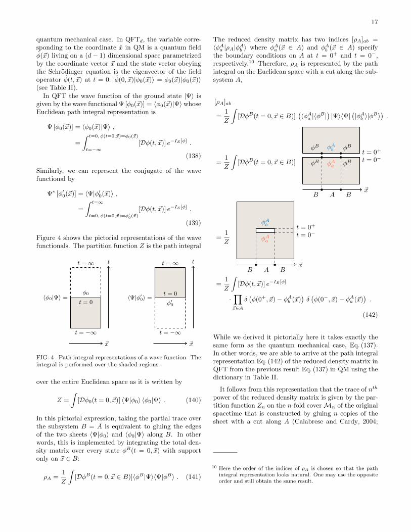
Figure 4 shows the pictorial representations of the wavefunctionals. The partition function Z is the path integral

t = 0

φ0

t = −∞

t =∞

〈φ0|Ψ〉 =

~x

t

t = 0

φ′0

t =∞

t = −∞

〈Ψ|φ′0〉 =

~x

t

FIG. 4 Path integral representations of a wave function. Theintegral is performed over the shaded regions.

over the entire Euclidean space as it is written by

Z =

∫[Dφ0(t = 0, ~x)] 〈Ψ|φ0〉 〈φ0|Ψ〉 . (140)

In this pictorial expression, taking the partial trace overthe subsystem B = A is equivalent to gluing the edgesof the two sheets 〈Ψ|φ0〉 and 〈φ0|Ψ〉 along B. In otherwords, this is implemented by integrating the total den-sity matrix over every state φB(t = 0, ~x) with supportonly on ~x ∈ B:

ρA =1

Z

∫[DφB(t = 0, ~x ∈ B)]〈φB |Ψ〉〈Ψ|φB〉 . (141)

The reduced density matrix has two indices [ρA]ab =〈φAa |ρA|φAb 〉 where φAa (~x ∈ A) and φAb (~x ∈ A) specifythe boundary conditions on A at t = 0+ and t = 0−,respectively.10 Therefore, ρA is represented by the pathintegral on the Euclidean space with a cut along the sub-system A,

[ρA]ab

=1

Z

∫[DφB(t = 0, ~x ∈ B)]

(〈φAa |〈φB |

)|Ψ〉〈Ψ|

(|φAb 〉|φB〉

),

=1

Z

∫[DφB(t = 0, ~x ∈ B)] φAa

φAbφB φB

φB φB

t = 0+

t = 0−

B A B~x

=1

Z

B A B~x

φAa

φAb t = 0+

t = 0−

=1

Z

∫[Dφ(t, ~x)] e−IE [φ]

·∏~x∈A

δ(φ(0+, ~x)− φAb (~x)

)δ(φ(0−, ~x)− φAa (~x)

).

(142)

While we derived it pictorially here it takes exactly thesame form as the quantum mechanical case, Eq. (137).In other words, we are able to arrive at the path integralrepresentation Eq. (142) of the reduced density matrix inQFT from the previous result Eq. (137) in QM using thedictionary in Table II.

It follows from this representation that the trace of nth

power of the reduced density matrix is given by the par-tition function Zn on the n-fold coverMn of the originalspacetime that is constructed by gluing n copies of thesheet with a cut along A (Calabrese and Cardy, 2004;

10 Here the order of the indices of ρA is chosen so that the pathintegral representation looks natural. One may use the oppositeorder and still obtain the same result.

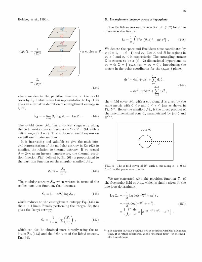
18

Holzhey et al., 1994),

trA(ρnA) =1

(Z)n

φA1

φA2

φA2

φA3

φAn

φA1

n copies ≡ Zn

=Zn

(Z)n,

(143)

where we denote the partition function on the n-foldcover by Zn. Substituting this representation to Eq. (119)gives an alternative definition of entanglement entropy inQFT,

SA = − limn→1

∂n(logZn − n logZ) . (144)

The n-fold cover Mn has a conical singularity alongthe codimension-two entangling surface Σ = ∂A with adeficit angle 2π(1−n). This is the most useful expressionwe will use in later sections.

It is interesting and valuable to give the path inte-gral representation of the modular entropy in Eq. (62) tomanifest the relation to thermal entropy. If we regardβ = 2πn as an inverse temperature, the thermal parti-tion function Z(β) defined by Eq. (61) is proportional tothe partition function on the singular manifold Mn,

Z(β) =Zn

(Z)n. (145)

The modular entropy Sn, when written in terms of thereplica partition function, then becomes

Sn = (1− n∂n) logZn , (146)

which reduces to the entanglement entropy Eq. (144) inthe n→ 1 limit. Finally performing the integral Eq. (65)gives the Renyi entropy,

Sn =1

1− nlog

(ZnZn

), (147)

which can also be obtained more directly using the re-lation Eq. (143) and the definition of the Renyi entropy,Eq. (54).

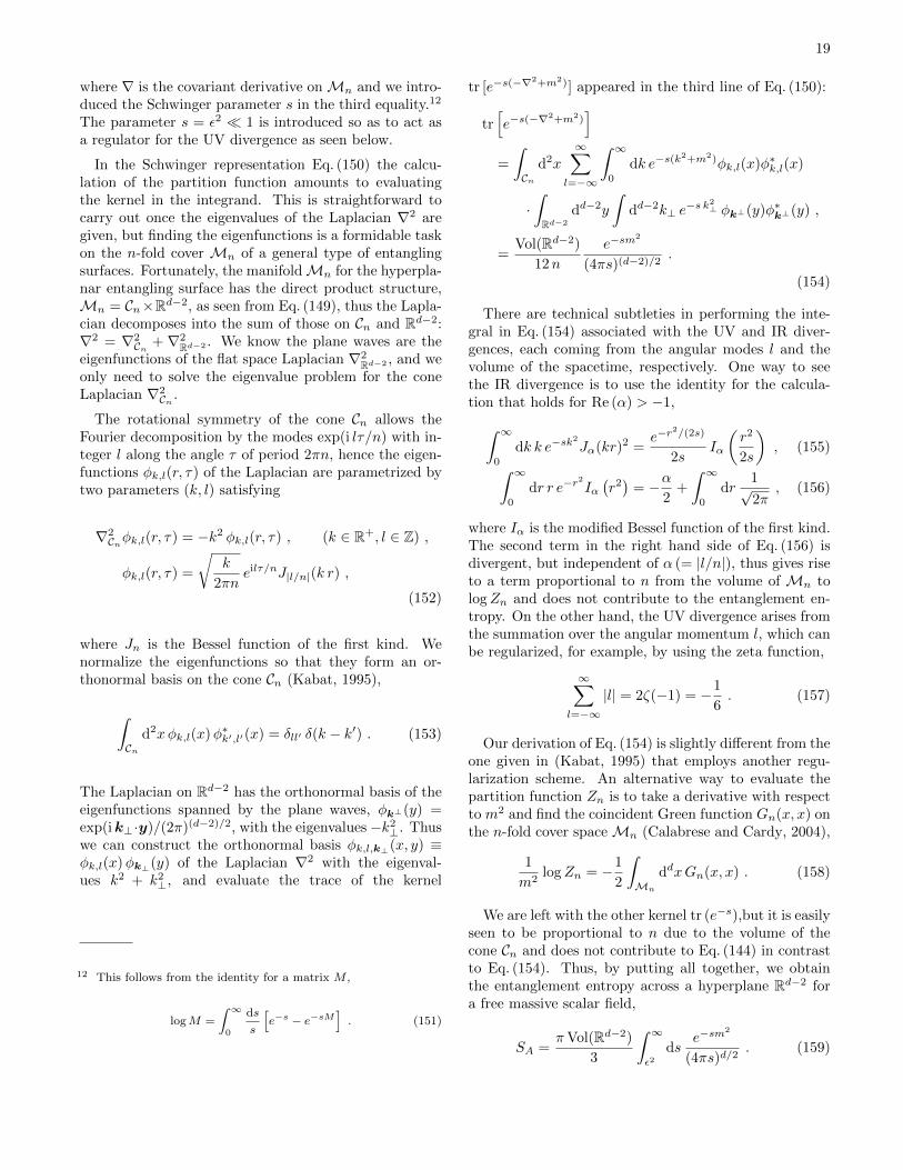
D. Entanglement entropy across a hyperplane

The Euclidean version of the action Eq. (107) for a freemassive scalar field is

IE =1

2

∫ddx

[(∂µφ)2 +m2φ2

]. (148)

We denote the space and Euclidean time coordinates byxi (i = 1, · · · , d − 1) and x0. Let A and B be regions inx1 > 0 and x1 ≤ 0, respectively. The entangling surfaceΣ is chosen to be a (d − 2)-dimensional hyperplane atx1 = 0: Σ = (x0, xi)|x0 = x1 = 0. Introducing themetric in the polar coordinates for the (x0, x1)-plane,

ds2 = dx20 + dx2

1 +

d−1∑i=2

dx2i ,

= dr2 + r2dτ2 +

d−1∑i=2

dx2i ,

(149)

the n-fold cover Mn with a cut along A is given by thesame metric with 0 ≤ r and 0 ≤ τ ≤ 2πn as shown inFig. 511. Hence the manifoldMn is the direct product ofthe two-dimensional cone Cn parametrized by (r, τ) andRd−2.

A

τ ∼ τ + 2πn

FIG. 5 The n-fold cover of Rd with a cut along x1 > 0 att = 0 in the polar coordinates.

We are concerned with the partition function Zn ofthe free scalar field onMn, which is simply given by theone-loop determinant,

logZn = −1

2log det(−∇2 +m2) ,

= −1

2tr log(−∇2 +m2) ,

=1

2

∫ ∞ε2

ds

str[e−s(−∇

2+m2) − e−s],

(150)

11 The angular variable τ should not be confused with the Euclideantime. It is rather considered as the “modular time” for the mod-ular Hamiltonian.

19

where ∇ is the covariant derivative onMn and we intro-duced the Schwinger parameter s in the third equality.12

The parameter s = ε2 1 is introduced so as to act asa regulator for the UV divergence as seen below.

In the Schwinger representation Eq. (150) the calcu-lation of the partition function amounts to evaluatingthe kernel in the integrand. This is straightforward tocarry out once the eigenvalues of the Laplacian ∇2 aregiven, but finding the eigenfunctions is a formidable taskon the n-fold cover Mn of a general type of entanglingsurfaces. Fortunately, the manifoldMn for the hyperpla-nar entangling surface has the direct product structure,Mn = Cn×Rd−2, as seen from Eq. (149), thus the Lapla-cian decomposes into the sum of those on Cn and Rd−2:∇2 = ∇2

Cn + ∇2Rd−2 . We know the plane waves are the

eigenfunctions of the flat space Laplacian ∇2Rd−2 , and we

only need to solve the eigenvalue problem for the coneLaplacian ∇2

Cn .

The rotational symmetry of the cone Cn allows theFourier decomposition by the modes exp(i lτ/n) with in-teger l along the angle τ of period 2πn, hence the eigen-functions φk,l(r, τ) of the Laplacian are parametrized bytwo parameters (k, l) satisfying

∇2Cnφk,l(r, τ) = −k2 φk,l(r, τ) , (k ∈ R+, l ∈ Z) ,

φk,l(r, τ) =

√k

2πneilτ/nJ|l/n|(k r) ,

(152)

where Jn is the Bessel function of the first kind. Wenormalize the eigenfunctions so that they form an or-thonormal basis on the cone Cn (Kabat, 1995),

∫Cn

d2xφk,l(x)φ∗k′,l′(x) = δll′ δ(k − k′) . (153)

The Laplacian on Rd−2 has the orthonormal basis of theeigenfunctions spanned by the plane waves, φk⊥(y) =exp(ik⊥ ·y)/(2π)(d−2)/2, with the eigenvalues −k2

⊥. Thuswe can construct the orthonormal basis φk,l,k⊥(x, y) ≡φk,l(x)φk⊥(y) of the Laplacian ∇2 with the eigenval-ues k2 + k2

⊥, and evaluate the trace of the kernel

12 This follows from the identity for a matrix M ,

logM =

∫ ∞0

ds

s

[e−s − e−sM

]. (151)

tr [e−s(−∇2+m2)] appeared in the third line of Eq. (150):

tr[e−s(−∇

2+m2)]

=

∫Cn

d2x

∞∑l=−∞

∫ ∞0

dk e−s(k2+m2)φk,l(x)φ∗k,l(x)

·∫Rd−2

dd−2y

∫dd−2k⊥ e

−s k2⊥ φk⊥(y)φ∗k⊥(y) ,

=Vol(Rd−2)

12n

e−sm2

(4πs)(d−2)/2.

(154)

There are technical subtleties in performing the inte-gral in Eq. (154) associated with the UV and IR diver-gences, each coming from the angular modes l and thevolume of the spacetime, respectively. One way to seethe IR divergence is to use the identity for the calcula-tion that holds for Re (α) > −1,∫ ∞

0

dk k e−sk2

Jα(kr)2 =e−r

2/(2s)

2sIα

(r2

2s

), (155)∫ ∞

0

dr r e−r2

Iα(r2)

= −α2

+

∫ ∞0

dr1√2π

, (156)

where Iα is the modified Bessel function of the first kind.The second term in the right hand side of Eq. (156) isdivergent, but independent of α (= |l/n|), thus gives riseto a term proportional to n from the volume of Mn tologZn and does not contribute to the entanglement en-tropy. On the other hand, the UV divergence arises fromthe summation over the angular momentum l, which canbe regularized, for example, by using the zeta function,

∞∑l=−∞

|l| = 2ζ(−1) = −1

6. (157)

Our derivation of Eq. (154) is slightly different from theone given in (Kabat, 1995) that employs another regu-larization scheme. An alternative way to evaluate thepartition function Zn is to take a derivative with respectto m2 and find the coincident Green function Gn(x, x) onthe n-fold cover spaceMn (Calabrese and Cardy, 2004),

1

m2logZn = −1

2

∫Mn

ddxGn(x, x) . (158)

We are left with the other kernel tr (e−s),but it is easilyseen to be proportional to n due to the volume of thecone Cn and does not contribute to Eq. (144) in contrastto Eq. (154). Thus, by putting all together, we obtainthe entanglement entropy across a hyperplane Rd−2 fora free massive scalar field,

SA =πVol(Rd−2)

3

∫ ∞ε2

dse−sm

2

(4πs)d/2. (159)

20

The UV divergent terms of the entanglement entropycan be read off by expanding it around ε = 0,

SA =Vol(Rd−2)

6(4π)d−1

[1

(d− 2)εd−2− m2

(d− 4)εd−4+ · · ·

].

(160)

The leading term is of order 1/εd−2 and the coefficientis proportional to the area of the entangling surfaceΣ = Rd−2. This is the manifestation of the area law ofentanglement entropy, one of the characteristics of quan-tum entanglement in QFTs. The subsequent terms areless divergent of order εd−2i with i = 1, 2, · · · . We willdiscuss these UV structures in a more general setting insection IV.F and show that they hold for any local quan-tum field theory on any manifold without boundary. It,however, should be noted that the area law does not holdin d = 2 dimensions where the entropy logarithmicallydiverges

SA = − 1

12log(m2ε2) . (161)

E. Rindler spacetime and thermofield double

The previous example of the entanglement entropyacross a hyperplane is not merely a simplest setup we cancarry out the exact calculation, but also has its physicalorigin in understanding a thermal aspect of black holesas an entanglement of a field across the horizon (Israel,1976; Laflamme, 1989).

To see their relation we analytically continue the met-ric Eq. (149) by Wick rotation τ = i η to the Rindlerspacetime

ds2 = −r2dη2 + dr2 +

d−1∑i=2

dx2i , (162)

with the new variable η ranging −∞ < η < ∞. TheRindler spacetime covers a portion specified by x1 ≥ |T |of the Minkowski spacetime R1,d−1 (see Fig. 6 for illus-tration),

ds2 = −dT 2 + dx21 +

d−1∑i=2

dx2i , (163)

as seen from the coordinate transformation

T = r sinh η , x1 = r cosh η . (164)

This transformation implies that an observer who is atrest in the Rindler spacetime is uniformly accelerating inthe Minkowski spacetime and is confined to the wedgex1 ≥ |T | separated by the “Rindler horizon” at r = 0from the rest of the spacetime. Hence at a given timeslice, say, T = 0, there is a region x1 < 0 (denoted by

B in Fig. 6) that is inaccessible to the Rindler observerliving on x1 > 0 (denoted by A in Fig. 6), whose stateis described by the reduced density matrix ρA that is amixed thermal ensemble at inverse temperature β = 2πeven if the total system A ∪ B is in a pure state. Thisis precisely the same situation we considered in the pre-vious subsection, and the entanglement entropy calcu-lated there is equivalent to the thermal entropy that theRindler observer measures in her/his frame.

x1AB

T

r=

0

η=∞

r=

0

η=−∞

η =const

r =const

FIG. 6 The Rindler spacetime (shaded region) embedded inthe Minkowski spacetime.

Now we want to give a concrete expression of the mod-ular Hamiltonian HA defined by Eq. (25) for the Rindlerobserver. In order to fix its form, we consider the matrixelement of the reduced density matrix ρA,

〈φ′A|ρA|φA〉 =1

Z〈φ′A|e−2πHA |φA〉 , (165)

and regard the right hand side as a transition amplitudefrom an initial state |φA〉 to a final state |φ′A〉. The (Eu-clidean) “time” evolution is generated by the modularHamiltonian HA over the period 2π. Looking back to theexample in the previous subsection, we can understandthat the system on the region A is time-evolved along theangular direction τ starting from τ = 0 to τ = 2π (seeFig. 5). We thus conclude the modular Hamiltonian inthe present case is the generator of the translation alongthe modular time τ , hence HA = ∂τ .13 In (Euclidean)QFT, the modular Hamiltonian is written explicitly bythe Noether’s theorem as

HA =

∫x0=0,x1≥0

dd−1xx1 T00 , (166)

13 In Lorentzian signature, the modular Hamiltonian generates theboost K = ∂η in the Rindler spacetime.

21

where Tµν is the stress tensor, which will be defined inEq. (209). This result is a particular case of the theoremby Bisognano and Wichmann (1975, 1976) that is validfor any QFT even with interactions.

Recalling the construction of the thermofield doublestate Eq. (24), we can rewrite the ground state wave func-tion in the Minkowski spacetime in the following form,

Ψ[φA, φB ] =1√Z

∑n

e−βEn/2ϕn[φA]ϕn[φB ] , (167)

where φA and φB are states on the time slice A and Brespectively, and ϕn[φ] is the nth eigenfunction of themodular Hamiltonian HA with eigenvalue En. Namely,we are able to purify a mixed state in the Rindler space-time to a pure state in the Minkowski spacetime by view-ing the region inside the Rindler horizon as a fictitioussystem (Israel, 1976; Laflamme, 1989).

F. Structure of UV divergences

In the previous section, we rewrite the definition ofentanglement entropy in terms of an (Euclidean) effec-tive action logZn on an n-fold cover Mn with a conicalsingularity along a codimension-two surface Σ = ∂A sur-rounding the region A of interest. In QFT on a curvedspacetime, the effective action is regarded as a functionof the metric gµν onMn, thus we are able to classify theUV divergent terms by diffeomorphism invariant localterms. Here we restrict our attention to QFTs withoutdimensionful parameters (= CFTs) for simplicity, whoseeffective action may be given by14

logZn[gµν ] =

[ d2 ]∑i=0

Cd−2i

∫Mn

ddx√gΛd−2iRi

+ (−1)d−12 F ,

(168)

where Λ is the UV cutoff scale of mass dimension one andRi is a scalar polynomial of the Riemann tensors of orderi onMn. We call F the renormalized free energy that isdimensionless and scheme independent constant in odddimensions. In contrast, there is a logarithmic divergence∼ C0 log Λ in addition to Eq. (168) in even dimensions,which makes the renormalized free energy ambiguous. Itis actually the source of the conformal anomaly and thecoefficient C0 depends on the central charges when thetheory is conformally invariant.

14 One can repeat the same argument presented here for any renor-malizable QFTs with a slight modification. For example, onecan add terms Λd−2M2,Λd−4M2R, · · · to the integrand if Mis a parameter of mass dimension one. This does not change theUV structure, and we ignore them for the moment.

We put aside the logarithmic divergence for a momentand determine the general structure of the UV diver-gences of entanglement entropy. We plug the generalform Eq. (168) into the formula Eq. (144), where thereappears only the difference logZn−n logZ of the effectiveactions for n close to 1. The UV divergent term of orderΛd−2i is proportional to the integral15

∫MnRi−n

∫MR

i

that should localize on the entangling surface Σ since then-fold covering space Mn differs from the original spaceM only around Σ. Especially, the leading divergencewith i = 0 cancels out because of Vol(Mn) = nVol(M1).We thus end up with the UV divergences in the entan-glement entropy starting from O(Λd−2):

SA = cd−2 Λd−2 + cd−4 Λd−4 + · · · , (169)

where cd−2i are given by the integrals of local diffeomor-phism invariants on Σ, schematically written as

cd−2i =∑

l+m=i−1

∫Σ

RlK2m , (170)

where K is the extrinsic curvature of Σ of order 2m,whose definition will be given in Eq. (190), and RlK2m

are scalar polynomials of R and K of order l and 2m re-spectively. The reason only even powers of the extrinsiccurvatures appear in Eq. (170) is that the entanglemententropy for a region A is equal to that of its complementA while their extrinsic curvatures have opposite signs,hence the odd powers of K vanish.

We have derived the UV structure Eq. (169) assum-ing the covariance and renormalizability of QFTs on amanifold without boundaries. If we relax the assump-tions, there are a variety of cases where entanglemententropy can take a different UV structure. For instance,(non-relativistic) systems with Fermi surfaces have theentanglement entropy that violates the area law loga-rithmically (Gioev and Klich, 2006; Wolf, 2006) (see also(Huijse et al., 2012; Ogawa et al., 2012) for the holo-graphic descriptions). For non-smooth entangling sur-faces such as those with corners and wedges, the entan-glement entropies have additional UV divergences whosecoefficients depend on the opening angles (Bueno andMyers, 2015; Bueno et al., 2015; Casini and Huerta, 2007;Casini et al., 2009; Elvang and Hadjiantonis, 2015; Frad-kin and Moore, 2006; Hirata and Takayanagi, 2007; Kle-banov et al., 2012b; Myers and Singh, 2012b).

The general structure Eq. (169) guarantees the UVfiniteness of the mutual information I(A,B) of two dis-joint systems A and B defined by Eq. (49) because everycoefficient cd−2i of the UV divergent term Λd−2i of the

15 We often use the shorthand notation for an integral∫M ≡∫

M ddx√g with the measure suppressed.

22

entanglement entropy is given by an integral on the en-tangling surface and they cancel in the mutual informa-tion due to the trivial identity (see Fig. 2)∫

ΣA+B

=

∫ΣA

+

∫ΣB

. (171)

We will fix the precise forms of the coefficients for freefields in the next section V. Note that there is a loga-rithmic divergence in even dimensions which we will sep-arately deal with when we discuss CFT in section VI.

V. HEAT KERNEL EXPANSION

The effective action logZn is a one-loop determinantprovided that a theory is non-interacting. The compu-tation of the effective action is carried out in a standardway using the heat kernel method (Birrell and Davies,1982). Here we reexamine a free massive scalar field ind dimensions on Mn using this method. The one-loopeffective action is given by

logZn = −1

2log det(D +m2) ,

=1

2

∫ ∞ε2

ds

strKMn

(s) e−m2s ,

(172)

where D is a scalar Laplacian plus the scalar curvatureD = −∇2 +ξR and m is the mass of the scalar field. Theparameter ξ is free, but becomes (d − 1)/(4d) when thetheory is conformally invariant (see section VI). In thesecond equality, we used the Schwinger representationand introduced the UV cutoff scale ε. The heat kerneloperator16 KMn

(s) = e−sD has the expansion arounds = 0 of the following form,

trKMn(s) =1

(4πs)d2

∞∑i=0

ai si . (173)

Note that the heat kernel coefficients ai do not dependon s. They decompose into the bulk and surface parts ona singular manifold Mn, and are assumed to allow theexpansion in the n→ 1 limit,

ai = abulki + (1− n) aΣ

i +O((1− n)2

). (174)

The bulk part abulki for the n-fold cover Mn is n times

larger than the one for the original space M1 as we willsee below,

abulki (Mn) = nabulk

i (M1) . (175)

16 The name follows from the fact that it satisfies the heat equation(∂s +D)KMn (s) = 0.

The subleading terms arise from the contributions of theconical singularity at the hypersurface Σ. Using theheat kernel expansion Eq. (173) in the effective actionEq. (172), we obtain the entanglement entropy as a powerseries of the inverse of the mass with the heat kernel co-efficients,

SA =1

2(4π)d2

∞∑i=0

aΣi

m2i−d Γ

(i− d

2,m2ε2

), (176)

where Γ(a, z) is the incomplete gamma function definedby Γ(t, x) =

∫∞x

ds st−1e−s. Hence given the surfaceparts of the heat kernel coefficients, the entanglemententropy is calculable at any order.

We will fix the heat kernel coefficients following thestrategy used by (Fursaev, 1994; Fursaev et al., 2013; Fur-saev and Solodukhin, 1995) (see also (Solodukhin, 2011)for a review). First, we start with the known results forthe bulk heat kernel coefficients on a non-singular mani-fold M (Birrell and Davies, 1982; Vassilevich, 2003):

abulk0 =

∫M

1 ,

abulk1 =

(1

6− ξ)∫MR ,

abulk2 =

∫M

[1

180R2µνρσ −

1

180R2µν

+1

2

(1

6− ξ)2

R2 +1

6

(1

5− ξ)∇2R

].

(177)

To obtain the surface parts, we regularize the conical sin-gularity at Σ and replaceMn with a regularized manifoldMn. The formulas Eq. (177) are valid for the smooth ge-

ometry Mn, from which we will read off the surface partsaΣi below.

A. Regularized cone with U(1) symmetry

Before presenting general cases, we consider a two-dimensional cone Cn with a conical singularity at theorigin (we will denote it by Σ),

ds2Cn = eσ(r)(dr2 + r2dτ2) ,

σ(r) = σ1r2 + σ2r

4 + · · · ,(178)

where 0 ≤ r , 0 ≤ τ ≤ 2πn, and σ1, σ2 are constant. Ithas a deficit angle 2π(1− n) at the tip.

In order to take into account the singularity properly,we regularize the cone by deforming the metric so thatthe origin at r = 0 becomes smooth while it has the samegeometry as Cn away from Σ. We call such a geometry aregularized cone Cn, letting the metric be

ds2Cn

= eσ(r)(fδ(r) dr2 + r2dτ2) , (179)

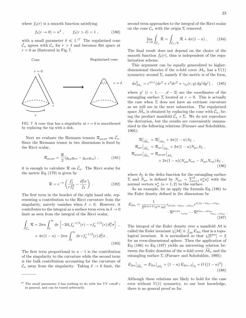
23

where fδ(r) is a smooth function satisfying

fδ(r → 0) = n2 , fδ(r > δ) = 1 , (180)

with a small parameter δ 1.17 The regularized coneCn agrees with Cn for r > δ and becomes flat space atr = 0 as illustrated in Fig. 7.

r = 0

r

τ

Cone

r = δ

Regularized cone

FIG. 7 A cone that has a singularity at r = 0 is smoothenedby replacing the tip with a disk.

Next we evaluate the Riemann tensors Rµνρσ on Cn.Since the Riemann tensor in two dimensions is fixed bythe Ricci scalar,

Rµνρσ =R2

(gµρgνσ − gµσgνρ) , (181)

it is enough to calculate R on Cn. The Ricci scalar forthe metric Eq. (179) is given by

R = e−σ(f ′δrf2δ

− ∂2rσ

fδ

). (182)

The first term in the bracket of the right hand side, rep-resenting a contribution to the Ricci curvature from thesingularity, naively vanishes when δ = 0. However, itcontributes to the integral as a surface term even in δ → 0limit as seen from the integral of the Ricci scalar,∫CnR = 2πn

∫ ∞0

dr[−2∂rf

−1/2δ (r)− rf−1/2

δ (r) ∂2rσ],

= 4π(1− n)− 2πn

∫ ∞0

dr rf−1/2δ (r) ∂2

rσ .

(183)

The first term proportional to n − 1 is the contributionof the singularity to the curvature while the second termis the bulk contribution accounting for the curvature ofCn away from the singularity. Taking δ → 0 limit, the

17 The small parameter δ has nothing to do with the UV cutoff εin general, and can be tuned arbitrarily.

second term approaches to the integral of the Ricci scalaron the cone Cn with the origin Σ removed:

limδ→0

∫CnR =

∫Cn/Σ

R+ 4π(1− n) , (184)

The final result does not depend on the choice of thesmooth function fδ(r), thus is independent of the regu-larization scheme.

This argument can be equally generalized to higher-dimensional theories if the n-fold cover Mn has a U(1)symmetry around Σ, namely if the metric is of the form,

ds2Mn

= eσ(r)(dr2 + r2dτ2 + γij(r, y) dyidyj) , (185)

where yi (i = 1, · · · , d − 2) are the coordinates of theentangling surface Σ located at r = 0. This is actuallythe case when Σ does not have an extrinsic curvatureas we will see in the next subsection. The regularizedspace Mn is obtained by replacing the cone with Cn, be-ing the product manifold Cn × Σ. We do not reproducethe derivation, but the results are conveniently summa-rized in the following relations (Fursaev and Solodukhin,1995):

R∣∣Mn

= R∣∣M1

+ 4π(1− n) δΣ ,

Rµν∣∣Mn

= Rµν∣∣M1

+ 2π(1− n)Nµν δΣ ,

Rµνρσ∣∣Mn

= Rµνρσ∣∣M1

+ 2π(1− n)(NµρNνσ −NµσNνρ) δΣ ,

(186)

where δΣ is the delta function for the entangling surfaceΣ and Nµν is defined by Nµν =

∑2a=1 n

aµn

aν with the

normal vectors naµ (a = 1, 2) to the surface.As an example, let us apply the formula Eq. (186) to

the Euler density defined in 2m dimensions by

E2m =1

22(m+1)πmm!εµ1µ2···µ2m−1µ2mε

ν1ν2···ν2m−1ν2m

· Rµ1µ2ν1ν2 · · ·R

µ2m−1µ2mν2m−1ν2m .

(187)

The integral of the Euler density over a manifold M iscalled the Euler invariant χ[M] ≡

∫ME2m that is a topo-

logical invariant. It is normalized so that χ[S2m] = 2for an even-dimensional sphere. Then the application ofEq. (186) to Eq. (187) yields an interesting relation be-

tween the Euler densities of the n-fold cover Mn and theentangling surface Σ (Fursaev and Solodukhin, 1995):

E2m

∣∣Mn

= E2m

∣∣M1

+ (1− n)E2m−2

∣∣Σ

+O((1− n)2

).

(188)

Although these relations are likely to hold for the caseeven without U(1) symmetry, to our best knowledge,there is no general proof so far.

24

B. Regularized cone without U(1) symmetry

Without a U(1) symmetry around the entangling sur-face, the metric can take a more general form thanEq. (185). If we parametrize the two-dimensional trans-verse directions to Σ by xa (a = 1, 2), the manifoldM looks like a product form R2 × Σ near the originx1 = x2 = 0. Even away from the origin, we can stillcontrol the metric in so called the Riemann normal co-ordinates (see e.g. (Fursaev et al., 2013; Lewkowycz andMaldacena, 2013; Rosenhaus and Smolkin, 2014)),

ds2M = δab dxadxb +

(γij(y) + 2Kaij xa

)dyidyj +O(x2) .

(189)

We introduced the extrinsic curvature Kaµν by

Kaµν = h ρµ h

σν ∇ρnaσ

∣∣Σ, (190)

where h is the induced metric on Σ, hµν = gµν −∑2a=1 n

aµn

aν with the unit normal vector naµ = δaµ to Σ.

Moving to the polar coordinates x1 = r sin τ, x2 = r cos τ ,the metric becomes

ds2M = dr2 + r2dτ2

+(γij(y) + 2r cos τ K1

ij + 2r sin τ K2ij

)dyidyj

+O(r2) .

(191)

The U(1) symmetry is broken due to the explicit de-pendence on the angular coordinate τ . Compared withEq. (185) for n = 1, the extrinsic curvatures Kaij has tovanish when the U(1) symmetry is present.

We want to calculate the integrals of geometric invari-ants on the n-fold cover as in the U(1) symmetric case.

To this end, we use the regularized n-fold cover Mn pro-posed by Fursaev et al. (2013),

ds2

M(FPS)n

= fδ(r)dr2 + r2dτ2

+[γij(y) + 2rnc1−n

(cos τ K1

ij + sin τ K2ij

)]dyidyj

+O(r2) ,

(192)

where τ ∼ τ + 2πn, c a constant of dimension of length,and fδ(r) is the smoothing function Eq. (180). Using theregularized metric, the following formulae for the inte-grals of the Riemann curvatures are argued to hold based

on several explicit calculations (Fursaev et al., 2013),∫Mn

R = n

∫MR+ 4π(1− n)

∫Σ

1 , (193)∫Mn

R2 = n

∫MR2 + 8π(1− n)

∫Σ

R , (194)∫Mn

R2µν = n

∫MR2µν

+ 4π(1− n)

∫Σ

[Raa −

1

2(Kaµµ )2

],

(195)∫Mn

R2µνρσ = n

∫MR2µνρσ

+ 8π(1− n)

∫Σ

[Rabab −KaµνKaµν

],

(196)

where the first one Eq. (193) is exact while only theterms up to O(1 − n) are shown in the rest. Thesubleading integral are performed on the codimension-two surface Σ and RΣ, Raa and Rabab are the Ricciscalar for the induced metric h, the induced Ricci ten-sor Raa =

∑a=1,2 n

aµn

aνRµν and the induced Riemann

tensor Rabab =∑a,b=1,2 n

aµn

bµn

aρn

bσRµνρσ, respectively.

These are enough to fix the heat kernel coefficients ai inEq. (177) up to the second order.

The results given in Eq. (193)-(196) can be used to de-rive similar relation to Eq. (188), but in the integratedforms in two and four dimensions:

χ[Mn] = χ[M] + (1− n)χ[Σ] +O((1− n)2

), (197)

where we used the fact that the regularized n-fold coverMn is topologically the same as the original manifoldM.

C. Heat kernel coefficients

We move onto the determination of the heat kernel co-efficients for the surface parts. Substituting the formu-lae Eq. (193)-(196) into the coefficients Eq. (177) on the

smooth geometry Mn, one finds the bulk parts satisfyEq. (175) and the surface parts become (Fursaev et al.,2013),

aΣ0 = 0 ,

aΣ1 =

2π(1− 6ξ)

3

∫Σ

1 ,

aΣ2 =

π

9

∫Σ

[1

5

(2Rabab −Raa − 2KaµνKaµν +

1

2(Kaµµ )2

)

+ (1− 6ξ)2R

],

(198)

25

where we used the Gauss-Codazzi equation to simplifythe expression,

R = RΣ + 2Raa −Rabab − (Kaµµ )2 +KaµνKaµν . (199)

It follows that the entanglement entropy Eq. (176) fora free massive scalar field has the UV divergences:

SA =AΣ

6(d− 2)εd−2+cd−4

εd−4+ · · ·+ γ(m) , (200)

where γ(m) includes all the mass dependences. The arealaw divergence can be found in the leading term thatcomes from the coefficient aΣ

1 proportional to the areaAΣ of the surface Σ. In addition, there is a universalterm proportional to the area in γ(m) (Hertzberg andWilczek, 2011):

γ(m) = γdAΣmd−2 + · · · , γd =

Γ(1− d/2)

12(4π)d/2−1.

(201)

The coefficient γd is finite for odd d, but is divergent dueto the pole of the gamma function for even d. This diver-gence signals the conformal anomaly in even dimensionsand modifies the mass expansion of γ(m) for even de,

γ(m) = γ(even)de

AΣmde−2 log(mε) + · · · ,

γ(even)de

=(−1)de/2−1

6(4π)de/2−1Γ(de/2).

(202)

This may be inferred from Eq. (201) by expanding itaround d = de − ε and using the replacement 1/ε →log(mε) for the pole in the dimensional regularization.

VI. CONFORMAL FIELD THEORY

In this section, we shall consider QFTs invariant underthe conformal transformation,

gµν(x′) = Ω2(x) gµν(x) , (203)

where gµν is the transformed metric. In Euclideanspace Rd, the group of the conformal transformation isSO(1, d+ 1) while, in Minkowski space R1,d−1, the groupis SO(2, d). The conformal group is an extension of thePoincare group, including the dilatation x′µ = λxµ fora constant λ and the special conformal transformationx′µ = (xµ + bµx2)/(1 + 2bµx

µ + b2x2) for a vector bµ,hence preserves the angle between two curves infinitesi-mally (Di Francesco et al., 1997).

Let IE [gµν , φ] is the (Euclidean) action for a theorywith a field φ(x) and a metric gµν . This theory is called(classical) conformal field theory (CFT) if the action doesnot change under the following transformation,

IE [gµν , φ] = IE [gµν , φ] , φ(x′) = Ω−∆(x)φ(x) ,(204)

for some constant ∆ being the conformal dimension ofthe field φ(x). For example, a scalar field theory coupledto a curved space

IE [gµν , φ] =1

2

∫ddx√g

[∂µφ∂

µφ+d− 2

4(d− 1)Rφ2

],

(205)

is conformally invariant with ∆ = d/2− 1. It is straight-forward to check the action Eq. (205) is conformal in-variant using the transformation law of the Ricci scalar(Birrell and Davies, 1982):

R[gµν ] = Ω−2R[gµν ]− 2(d− 1)Ω−3∇2Ω

− (d− 1)(d− 4)Ω−4∂µΩ ∂µΩ ,(206)

where the covariant derivatives in the right hand side aretaken with respect to the metric gµν before the conformaltransformation. An equivalent, but a slightly simpler wayto derive Eq. (205) is to construct a conformal invariantφd/∆

√gR[φ2/∆gµν ] out of the metric and the scalar field,

and use Eq. (206) with Ω = φ1/∆. To make it quadraticin φ, one needs to set ∆ = d/2 − 1 for the conformaldimension (Brown, 1977), and finds

φd/∆R[φ2/∆gµν ] = φ2R[gµν ]

+4(d− 1)

d− 2[∂µφ∂

µφ−∇µ(φ∂µφ)] .

(207)

This gives the conformal invariant action Eq. (205) up tothe total derivative and normalization.

Next, consider an action IE [gµν ] of the metric, whichmay be obtained by integrating out all fields on a curvedspace. The variation of the action under the infinitesimalconformal transformation δgµν = 2 δΩ(x)gµν becomes

δIE [gµν ] =

∫ddx δgµν

δIE [gµν ]

δgµν=

∫ddx√g T µ

µ δΩ(x) ,

(208)

where the stress-energy tensor is defined by

Tµν =2√g

δIEδgµν

. (209)

If the theory is conformally invariant, the action has to beinvariant under any deformation δΩ(x), hence the traceof the stress-energy tensor has to vanishes, T µ

µ = 0.The traceless property of the stress tensor at the classi-

cal level is violated at the quantum mechanical level dueto the conformal anomaly in even dimensions (Deser andSchwimmer, 1993; Duff, 1994), which can be put, up toscheme-dependent total derivative terms, in the form,

〈T µµ 〉 =

(−1)d2

2AEd −

∑i

Bi Ii , (210)

26

where Ed is the Euler density, normalized so that∫Sd Ed = 2, and Ii are a set of the independent Weyl

invariants build from the Weyl tensor in d dimensions.The coefficients A and Bi are referred to as the type Aand B central charges, respectively.

A. Correlation functions

The conformal symmetry restricts the form of correla-tion functions more severely than the Poincare symme-try. We start with a primary scalar operator O(x) ofconformal dimension ∆ transforming under the confor-mal transformation Eq. (203) as

O(x′) = Ω−∆(x)O(x) . (211)

The translation invariance imposes the constancy of theone-point function, 〈O(x)〉 = c, but the scaling lawEq. (211) implies c = Ω−∆(x) c for any Ω(x), thus theone-point function vanishes:

〈O(x)〉 = 0 . (212)

Similarly the two-point function 〈O1(x)O2(y)〉 of pri-mary operators O1 and O2 of conformal dimensions ∆1

and ∆2 only depends on the distance |x− y| between thetwo points by the translation invariance. To incorporatethe dilatation and the special conformal invariances, thetwo conformal dimensions should be the same. Then thetwo-point function of appropriately normalized operatorstakes the form

〈O1(x)O2(y)〉 =δ∆1 ∆2

|x− y|2∆1. (213)

The three-point function of primary operators O1,O2

and O3 of conformal dimensions ∆1,∆2 and ∆3 are sim-ilarly fixed by the conformal symmetry,

〈O1(x)O2(y)O3(z)〉

=C123

|x− y|∆1+∆2−∆3 |y − z|∆2+∆3−∆1 |z − x|∆3+∆1−∆2,

(214)

where C123 is an undetermined constant. Correlationfunctions of more than four operators cannot be com-pletely fixed by only the conformal invariance in this way.

For conserved currents jµ(x) of dimension ∆ = d − 1and the stress-tensor Tµν(x) of dimension d, their one-point functions vanish and the two-point functions arefixed to be (Erdmenger and Osborn, 1997; Osborn andPetkou, 1994)

〈jµ(x) jν(y)〉 = CJIµν(x− y)

(x− y)2(d−1), (215)

and

〈Tµν(x)Tρσ(y)〉 = CTIµν,ρσ(x− y)

(x− y)2d, (216)

with the conformally invariant functions,

Iµν(x) = δµν −2xµxνx2

,

Iµν,ρσ(x) =1

2(Iµρ(x)Iνσ(x) + Iµσ(x)Iνρ(x))− 1

dδµνδρσ .

(217)

The two-point functions of a scalar primary field O(x)and the conserved current or the stress-tensor vanish,

〈j(x)O(y)〉 = 〈Tµν(x)O(y)〉 = 0 , (218)

due to the conformal invariance and the conservationlaws ∂µj

µ = 0 and ∂µTµν = 0.

B. Conformal anomaly in entanglement entropy

We saw in the previous section that entanglement en-tropy has the UV divergences whose leading part is al-ways proportional to the area of the entangling surfaceΣ in Eq. (200). There are also universal logarithmic di-vergences depending on whether d is even or not. Wewill show this logarithmic divergence is induced by theconformal anomaly Eq. (210) of the stress-energy tensorin even d dimensions.

Let us consider the scale transformation of entangle-ment entropy of an entangling surface Σ of size l. Weneed to know how the partition function Zn on then-fold cover Mn transforms under the Weyl scaling,l → eσl. Equivalently we act the scaling of the met-ric gµν → e2σgµν on the effective action logZn and readoff the variation locally given by the expectation value ofthe stress-tensor on Mn

ld

dllogZn = −

∫Mn

ddx√g 〈T µ

µ 〉 . (219)

It follows with the QFT definition Eq. (144) that the en-tanglement entropy varies under the scale transformationas

ld

dlSA = −

∫M1

ddx√g 〈T µ

µ 〉+ limn→1

∂n

∫Mn

ddx√g 〈T µ

µ 〉 .

(220)

In odd dimensions, 〈T µµ 〉 = 0 for CFTs and there are

no logarithmic divergences in the entropy. On the otherhand, the right hand side can be non-vanishing due tothe conformal anomaly, Eq. (210), in even dimensions. Ifa theory is defined on a flat space (M1 = Rd), the firstterm always vanishes while the second term has a non-trivial contribution from the conical singularity at theentangling surface Σ. In what follows, we will estimatethe second term explicitly using the formulae Eq. (193)-(196) in two and four dimensions.

In two dimensions, the Euler density is E2 = R/(4π)while there are no Weyl invariants. We rescale the type

27

A central charge, A = c/3, so as to follow the canonicalconvention in CFT2. Then substituting the trace of thestress-tensor

〈T µµ 〉 = − c

24πR , (221)

into Eq. (220) and applying the formula Eq. (193), we findthe entanglement entropy for an interval of width l,

ld

dlSA =

c

6

∫Σ

1 =c

3. (222)

This result yields a well-known behavior of entanglemententropy of CFT2 (Calabrese and Cardy, 2004; Holzheyet al., 1994; Jin and Korepin, 2004)

SA =c

3log

l

ε+ · · · , (223)

where ε is a UV cutoff and · · · are finite parts.In four dimensions, there are one Euler density and

one Weyl invariant,

E4 =1

32π2

(R2µνρσ − 4R2

µν +R2),

I4 =1

16π2

(R2µνρσ − 2R2

µν +1

3R2

),

(224)

whose coefficients we conventionally take to be A = aand B = c, respectively. Again, the formulae Eq. (193)-(196) and the identities Eq. (210) and Eq. (220) lead tothe logarithmic divergence of entanglement entropy inCFT4:

SA =c2ε2

+ c0 logl

ε+ · · · , (225)

where c2 is a constant proportional to the area AΣ of theentangling surface Σ and c0 is fixed to be (Fursaev et al.,2013; Solodukhin, 2008)

c0 = −a2χ[Σ]

+c

2π

∫Σ

[Rabab −Raa +

1

3R

+1

2(Kaµµ )2 −KaµνKaµν

].

(226)

Here we used the Gauss-Codazzi equation Eq. (199) relat-ing the Ricci curvature on Σ to the intrinsic and extrinsiccurvatures, which gives the first term proportional to thetopological invariant (the Euler characteristic)

χ[Σ] =

∫Σ

E2 =1

4π

∫Σ

RΣ , (227)

of the entangling surface Σ. If the entangling surfaceis spherical, Σ = S2, only the a-anomaly contributes toEq. (226), while if it is cylindrical Σ = S1 × R, only thec-anomaly survives. The same expression (226) for the

coefficient c0 can be obtained by a holographic calcula-tion in higher derivative gravities (Hung et al., 2011a),where the logarithmic divergences arise from a particularclass of anomalies for a submanifold of even dimensionsin CFT, known as Graham-Witten anomalies (Grahamand Witten, 1999).

In higher dimensions, there are one Euler density andseveral independent Weyl invariants. Entanglement en-tropy in even d-dimensional CFT allows the structure,

SA =cd−2

εd−2+cd−4

εd−4+ · · ·+ c2

ε2+ c0 log

l

ε+ · · · , (228)

with the logarithmic coefficient given by

c0 =(−1)d/2+1

2Aχ[Σ]−

∑i

Bi

(∂n

∫Mn

Ii

) ∣∣∣∣n→1

.

(229)

The finite terms represented by the last dots depend onthe regularization scheme and do not have any physicalmeaning. On the other hand, entanglement entropy inodd d-dimensional CFT has similar expansions withoutthe logarithmic term,

SA =cd−2

εd−2+cd−4

εd−4+ · · ·+ c1

ε+ (−1)(d−1)/2F . (230)

The finite part F is scheme independent and physicalobservable. The sign factor (−1)(d−1)/2 is introducedfor F being positive in d dimensions (Klebanov et al.,2011), but there are no proofs for the positivity exceptfor topological field theory where F is the topological en-tanglement entropy that can be shown to be non-negative(Kitaev and Preskill, 2006; Levin and Wen, 2006). Wewill investigate the role of the finite part of entanglemententropy in odd dimensions in later sections.

1. One interval in CFT2

One can derive the entanglement entropy of one in-terval Eq. (223) in CFT2 on a flat space C using purelyCFT techniques. Suppose the interval is placed betweenz = −l/2 and z = l/2 in the complex z-plane C. We firstmap the interval to a semi-infinite line from the origin tothe infinity by the transformation

ζ ≡ z + l/2

z − l/2. (231)

Then we make use of the conformal transformation fromthe complex plane to a cylinder,

w ≡ τ + iϕ =`

2πlog ζ , (232)

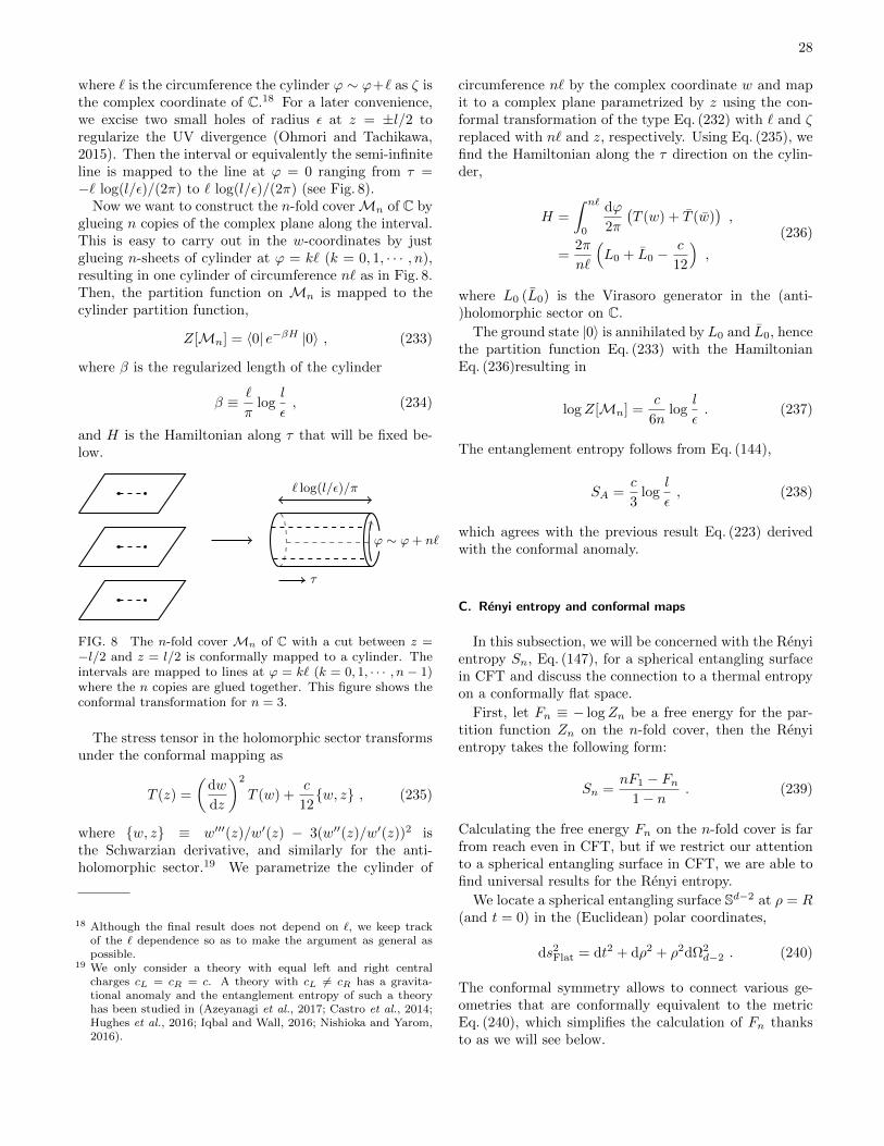
28

where ` is the circumference the cylinder ϕ ∼ ϕ+` as ζ isthe complex coordinate of C.18 For a later convenience,we excise two small holes of radius ε at z = ±l/2 toregularize the UV divergence (Ohmori and Tachikawa,2015). Then the interval or equivalently the semi-infiniteline is mapped to the line at ϕ = 0 ranging from τ =−` log(l/ε)/(2π) to ` log(l/ε)/(2π) (see Fig. 8).

Now we want to construct the n-fold coverMn of C byglueing n copies of the complex plane along the interval.This is easy to carry out in the w-coordinates by justglueing n-sheets of cylinder at ϕ = k` (k = 0, 1, · · · , n),resulting in one cylinder of circumference n` as in Fig. 8.Then, the partition function on Mn is mapped to thecylinder partition function,

Z[Mn] = 〈0| e−βH |0〉 , (233)

where β is the regularized length of the cylinder

β ≡ `

πlog

l

ε, (234)

and H is the Hamiltonian along τ that will be fixed be-low.

τ

ϕ ∼ ϕ+ n`

` log(l/ε)/π

FIG. 8 The n-fold cover Mn of C with a cut between z =−l/2 and z = l/2 is conformally mapped to a cylinder. Theintervals are mapped to lines at ϕ = k` (k = 0, 1, · · · , n − 1)where the n copies are glued together. This figure shows theconformal transformation for n = 3.

The stress tensor in the holomorphic sector transformsunder the conformal mapping as

T (z) =

(dw

dz

)2

T (w) +c

12w, z , (235)

where w, z ≡ w′′′(z)/w′(z) − 3(w′′(z)/w′(z))2 isthe Schwarzian derivative, and similarly for the anti-holomorphic sector.19 We parametrize the cylinder of

18 Although the final result does not depend on `, we keep trackof the ` dependence so as to make the argument as general aspossible.

19 We only consider a theory with equal left and right centralcharges cL = cR = c. A theory with cL 6= cR has a gravita-tional anomaly and the entanglement entropy of such a theoryhas been studied in (Azeyanagi et al., 2017; Castro et al., 2014;Hughes et al., 2016; Iqbal and Wall, 2016; Nishioka and Yarom,2016).

circumference n` by the complex coordinate w and mapit to a complex plane parametrized by z using the con-formal transformation of the type Eq. (232) with ` and ζreplaced with n` and z, respectively. Using Eq. (235), wefind the Hamiltonian along the τ direction on the cylin-der,

H =

∫ n`

0

dϕ

2π

(T (w) + T (w)

),

=2π

n`

(L0 + L0 −

c

12

),

(236)

where L0 (L0) is the Virasoro generator in the (anti-)holomorphic sector on C.

The ground state |0〉 is annihilated by L0 and L0, hencethe partition function Eq. (233) with the HamiltonianEq. (236)resulting in

logZ[Mn] =c

6nlog

l

ε. (237)

The entanglement entropy follows from Eq. (144),

SA =c

3log

l

ε, (238)

which agrees with the previous result Eq. (223) derivedwith the conformal anomaly.

C. Renyi entropy and conformal maps

In this subsection, we will be concerned with the Renyientropy Sn, Eq. (147), for a spherical entangling surfacein CFT and discuss the connection to a thermal entropyon a conformally flat space.

First, let Fn ≡ − logZn be a free energy for the par-tition function Zn on the n-fold cover, then the Renyientropy takes the following form:

Sn =nF1 − Fn

1− n. (239)

Calculating the free energy Fn on the n-fold cover is farfrom reach even in CFT, but if we restrict our attentionto a spherical entangling surface in CFT, we are able tofind universal results for the Renyi entropy.

We locate a spherical entangling surface Sd−2 at ρ = R(and t = 0) in the (Euclidean) polar coordinates,

ds2Flat = dt2 + dρ2 + ρ2dΩ2

d−2 . (240)

The conformal symmetry allows to connect various ge-ometries that are conformally equivalent to the metricEq. (240), which simplifies the calculation of Fn thanksto as we will see below.

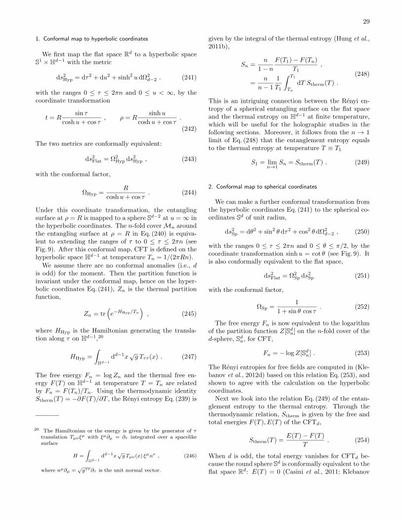
29

1. Conformal map to hyperbolic coordinates

We first map the flat space Rd to a hyperbolic spaceS1 ×Hd−1 with the metric

ds2Hyp = dτ2 + du2 + sinh2 udΩ2

d−2 . (241)

with the ranges 0 ≤ τ ≤ 2πn and 0 ≤ u < ∞, by thecoordinate transformation

t = Rsin τ

coshu+ cos τ, ρ = R

sinhu

coshu+ cos τ.

(242)

The two metrics are conformally equivalent:

ds2Flat = Ω2

Hyp ds2Hyp , (243)

with the conformal factor,

ΩHyp =R

coshu+ cos τ. (244)

Under this coordinate transformation, the entanglingsurface at ρ = R is mapped to a sphere Sd−2 at u =∞ inthe hyperbolic coordinates. The n-fold coverMn aroundthe entangling surface at ρ = R in Eq. (240) is equiva-lent to extending the ranges of τ to 0 ≤ τ ≤ 2πn (seeFig. 9). After this conformal map, CFT is defined on thehyperbolic space Hd−1 at temperature Tn = 1/(2πRn).

We assume there are no conformal anomalies (i.e., dis odd) for the moment. Then the partition function isinvariant under the conformal map, hence on the hyper-bolic coordinates Eq. (241), Zn is the thermal partitionfunction,

Zn = tr(e−HHyp/Tn

), (245)

where HHyp is the Hamiltonian generating the transla-tion along τ on Hd−1,20

HHyp =

∫Hd−1

dd−1x√g Tττ (x) . (247)

The free energy Fn = logZn and the thermal free en-ergy F (T ) on Hd−1 at temperature T = Tn are relatedby Fn = F (Tn)/Tn. Using the thermodynamic identityStherm(T ) = −∂F (T )/∂T , the Renyi entropy Eq. (239) is

20 The Hamiltonian or the energy is given by the generator of τtranslation Tµνξµ with ξµ∂µ = ∂τ integrated over a spacelikesurface

H =

∫Hd−1

dd−1x√g Tµν(x) ξµnν , (246)

where nµ∂µ =√gττ∂τ is the unit normal vector.

given by the integral of the thermal entropy (Hung et al.,2011b),

Sn =n

1− nF (T1)− F (Tn)

T1,

=n

n− 1

1

T1

∫ T1

Tn

dT Stherm(T ) .

(248)

This is an intriguing connection between the Renyi en-tropy of a spherical entangling surface on the flat spaceand the thermal entropy on Hd−1 at finite temperature,which will be useful for the holographic studies in thefollowing sections. Moreover, it follows from the n → 1limit of Eq. (248) that the entanglement entropy equalsto the thermal entropy at temperature T ≡ T1

S1 = limn→1

Sn = Stherm(T ) . (249)

2. Conformal map to spherical coordinates

We can make a further conformal transformation fromthe hyperbolic coordinates Eq. (241) to the spherical co-ordinates Sd of unit radius,

ds2Sp = dθ2 + sin2 θ dτ2 + cos2 θ dΩ2

d−2 , (250)

with the ranges 0 ≤ τ ≤ 2πn and 0 ≤ θ ≤ π/2, by thecoordinate transformation sinhu = cot θ (see Fig. 9). Itis also conformally equivalent to the flat space,

ds2Flat = Ω2

Sp ds2Sp (251)

with the conformal factor,

ΩSp =1

1 + sin θ cos τ. (252)

The free energy Fn is now equivalent to the logarithmof the partition function Z[Sdn] on the n-fold cover of thed-sphere, Sdn, for CFT,

Fn = − logZ[Sdn] . (253)

The Renyi entropies for free fields are computed in (Kle-banov et al., 2012d) based on this relation Eq. (253), andshown to agree with the calculation on the hyperboliccoordinates.

Next we look into the relation Eq. (249) of the entan-glement entropy to the thermal entropy. Through thethermodynamic relation, Stherm is given by the free andtotal energies F (T ), E(T ) of the CFTd,

Stherm(T ) =E(T )− F (T )

T. (254)

When d is odd, the total energy vanishes for CFTd be-cause the round sphere Sd is conformally equivalent to theflat space Rd: E(T ) = 0 (Casini et al., 2011; Klebanov

30

t

ρ

Sd−2

Rd

ds2Flat = dt2 + dρ2 + ρ2 dΩ2d−2

τ

Sd−2

u

S1 ×Hd−1

ds2Hyp = dτ2 + du2 + sinh2 u dΩ2d−2

Sd−2

τ

θ = 0 π/2

Sd

ds2Sp = dθ2 + sin2 θ dτ2 + cos2 θ dΩ2d−2

FIG. 9 The coordinate transformation Eq. (242) induces the conformal map from a flat space to a hyperbolic space times acircle. The latter is further conformally mapped to a sphere by the coordinate transformation, sinhu = cot θ. The blue circlesrepresent the entangling surface Sd−2, and the orange arrows stand for the modular time, respectively.

et al., 2012d). Combining the two relations Eq. (249)and Eq. (254) with F (T1)/T1 = F1 = − logZ[Sdn], we ob-tain the equality between the entanglement entropy of asphere Sd−2 and the partition function on Sd,

S1 = logZ[Sd] . (255)

Note that this equality should be taken up to UV di-vergences as the vanishing of the total energy holds forCFTd only after renormalizing the divergences. If theright hand side is the correctly renormalized effective ac-tion, it should be identified with the universal part of theentanglement entropy in Eq. (230),

F = (−1)d−12 logZ[Sd] . (256)

This will be the key relation in section VIII when weconstruct a monotonically decreasing function along RGflows in odd dimensions.

When d is even, there are conformal anomalies in thepartition function Z[Sd], which gives rise to the logarith-mic divergence in entanglement entropy as appeared inEq. (228). This is most easily seen by analytically contin-uing the relation Eq. (255) from odd to even dimensionsand replacing the pole with the logarithm.

D. Universal behavior of Renyi entropy in CFT

Having established the universal relation Eq. (255) forthe spherical entanglement entropy, we will now seek forthe universal aspects of the Renyi entropies. We will setR = 1 below since the result should not depend on Rbecause of the conformal symmetry.

We want to examine the universal part of the sphericalRenyi entropy in odd dimensions, and expand it aroundn = 1 where S1 = −F1 up to the UV divergences. From

Eq. (239) we have the expansion,

Sn = S1 +Fn − F1

n− 1,

= S1 +

∞∑k=1

1

k!

∂kFn∂nk

∣∣∣∣n=1

(n− 1)k−1 .(257)

For a spherical entangling surface in CFT, the free en-ergy is given by the partition function Eq. (245) on thehyperbolic coordinates, which fixes the derivatives of Fn,

∂kFn∂nk

∣∣∣∣n=1

= −(−2π)k〈HkHyp〉 , (258)

where 〈 · 〉 ≡ tr( · e−2πHHyp)/tr(e−2πHHyp) stands for theexpectation value of an operator and we used the factthat the energy vanishes for CFT in odd dimensions:E(T ) = 〈HHyp〉 = 0. The form of the HamiltonianEq. (247) on the hyperbolic space allows us to obtain theexpansion in terms of the correlation functions of thestress tensors,

Sn = S1

−∞∑k=1

(−2π)k+1

(k + 1)!(n− 1)k

·∫Hd−1

· · ·∫Hd−1

k+1∏i=1

dd−1xi√g 〈Tττ (x1) · · ·Tττ (xk+1)〉 .

(259)

The leading term is fixed by the two-point function ofthe stress tensors, whose integral results in (Perlmutter,2014)

∂nSn∣∣n=1

= −CT Vol(Hd−1

) πd/2+1(d− 1)Γ (d/2)

Γ(d+ 2),

(260)

31

where CT is a constant present in Eq. (216). For odd d,the regularized volume of Hd−1 is (see (Klebanov et al.,2012d) for d = 3)

Vol(Hd−1) = (−1)(d−1)/2 πd/2

Γ (d/2)= πd/2−1Γ(1− d/2) ,

(261)

which may be obtained by putting the cutoff Λ 1 atthe spatial infinity of Hd−1 and picking up a constantterm in Λ→∞ limit.21

While the universal result Eq. (260) was derived underthe assumption that d is odd, it is shown to hold for evend (Perlmutter, 2014) where there are additional terms in-cluding the one-point function 〈H〉 which no longer van-ishes due to the conformal anomaly. In addition, the vol-ume of the hyperbolic space Vol(Hd−1) logarithmicallydiverges for even d after regularizing the power law di-vergence, which may be inferred from Eq. (261) as a poleof the gamma function by analytically continuing odd dto even.

We finally note that the first derivative of the sphereentanglement entropy Eq. (260) can be useful to read offthe coefficient CT of the two-point function of the stresstensor. A similar expansion and a universal leading co-efficient will be derived for a supersymmetric generaliza-tion of the Renyi entropy in section VIII.G.

VII. HOLOGRAPHIC METHOD

The holographic principle, stating the equivalence be-tween gauge theory and gravity theory, is implied bystring theory. One of the most famous duality isthe AdS/CFT correspondence conjectured by Maldacena(1998), which has been the main focus of research in highenergy theory for two decades. String theory has ex-tended objects called D-branes that allows two comple-mentary descriptions as a black hole in general relativityand a gauge theory on the world-volume. In the formerpicture, one finds the Anti-de-Sitter (AdS) geometry inthe near horizon region, which turns out to be equivalentto the gauge theory of the latter picture. The AdS/CFTcorrespondence crystalizes the equivalence by connectingthe type IIB superstring theory on the AdS space with asupersymmetric CFT living on the boundary of the AdSspace. This is a concrete example of duality where astrongly-coupled region of one theory is described by aweakly-couple region of the other theory. Hence the di-rect check of this correspondence is far reach in its natureand remains to be proved.

21 In the second equality, we used the reflection formula for thegamma functions, Γ(z)Γ(1− z) = π/ sin(πz) = π(−1)(d−1)/2.

Apart from the string theory implication, we can takethe AdS/CFT correspondence as a gauge/gravity dualityin its own right simply based on the symmetry argumentthat the isometry SO(2, d) of the AdSd+1 space agreeswith the conformal group of CFTd.

In this section, we will give a quick review of theAdS/CFT correspondence. This subject is comprehen-sively covered by an excellent review paper (Aharonyet al., 2000) and many other literatures including (Kle-banov, 2000; McGreevy, 2010) from different point ofviews. We will then introduce the holographic formula ofentanglement entropy proposed by Ryu and Takayanagi(2006a,b) and discuss the implications. The reviews onentanglement entropy from the holographic point of viewcan be found in (Nishioka et al., 2009; Rangamani andTakayanagi, 2017; Takayanagi, 2012).

A. The AdS geometries

We briefly sketch several types of the useful coordi-nates for the AdS geometry that we will adopt from timeto time in the following sections. Table III is the sum-mary of the relations between the AdS coordinates andthe corresponding conformally flat spaces on their bound-aries.

To begin with, consider the flat (d + 2)-dimensionalpseudo Euclidean space defined by

ds2 = −dy2−1 − dy2

0 + dy21 + · · ·+ dy2

d . (262)

The AdSd+1 space with radius L is an embedding hyper-surface satisfying

−y2−1 − y2

0 + y21 + · · ·+ y2

d = −L2 . (263)

The above construction manifests the isometry SO(2, d)of the AdSd+1 space. Among many coordinates in theAdS space we focus on the typical examples, the global,Poincare and hyperbolic coordinates below.

1. Global coordinates

The global coordinates are introduced by the coordi-nate transformations:

y−1 = L cosh ρ sin τ ,

y0 = L cosh ρ cos τ ,

yi = L sinh ρ ei , (i = 1, . . . , d) ,

(264)

where ei satisfy the relation∑di=1(ei)2 = 1 and span a d-

dimensional sphere. The metric Eq. (262) then becomes

ds2 = L2[− cosh2 ρdτ2 + dρ2 + sinh2 ρdΩ2

d−1

]. (265)

By the coordinate transformation t ≡ Lτ, sinh ρ = r/L,we find another form of the global coordinates often used

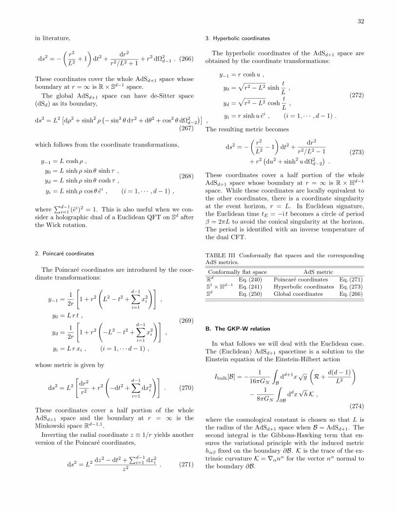
32

in literature,

ds2 = −(r2

L2+ 1

)dt2 +

dr2

r2/L2 + 1+ r2 dΩ2

d−1 . (266)

These coordinates cover the whole AdSd+1 space whoseboundary at r =∞ is R× Sd−1 space.

The global AdSd+1 space can have de-Sitter space(dSd) as its boundary,

ds2 = L2[dρ2 + sinh2 ρ

(− sin2 θ dτ2 + dθ2 + cos2 θ dΩ2

d−2

)],

(267)

which follows from the coordinate transformations,

y−1 = L cosh ρ ,

y0 = L sinh ρ sin θ sinh τ ,

yd = L sinh ρ sin θ cosh τ ,

yi = L sinh ρ cos θ ei , (i = 1, · · · , d− 1) ,

(268)

where∑d−1i=1 (ei)2 = 1. This is also useful when we con-

sider a holographic dual of a Euclidean QFT on Sd afterthe Wick rotation.

2. Poincare coordinates

The Poincare coordinates are introduced by the coor-dinate transformations:

y−1 =1

2r

[1 + r2

(L2 − t2 +

d−1∑i=1

x2i

)],

y0 = Lr t ,

yd =1

2r

[1 + r2

(−L2 − t2 +

d−1∑i=1

x2i

)],

yi = Lr xi , (i = 1, · · · d− 1) ,

(269)

whose metric is given by

ds2 = L2

[dr2

r2+ r2

(−dt2 +

d−1∑i=1

dx2i

)]. (270)

These coordinates cover a half portion of the wholeAdSd+1 space and the boundary at r = ∞ is theMinkowski space Rd−1,1.

Inverting the radial coordinate z ≡ 1/r yields anotherversion of the Poincare coordinates,

ds2 = L2 dz2 − dt2 +∑d−1i=1 dx2

i

z2. (271)

3. Hyperbolic coordinates

The hyperbolic coordinates of the AdSd+1 space areobtained by the coordinate transformations:

y−1 = r coshu ,

y0 =√r2 − L2 sinh

t

L,

yd =√r2 − L2 cosh

t

L,

yi = r sinhu ei , (i = 1, · · · , d− 1) .

(272)

The resulting metric becomes

ds2 = −(r2

L2− 1

)dt2 +

dr2

r2/L2 − 1

+ r2(du2 + sinh2 udΩ2

d−2

).

(273)

These coordinates cover a half portion of the wholeAdSd+1 space whose boundary at r = ∞ is R × Hd−1

space. While these coordinates are locally equivalent tothe other coordinates, there is a coordinate singularityat the event horizon, r = L. In Euclidean signature,the Euclidean time tE = −i t becomes a circle of periodβ = 2πL to avoid the conical singularity at the horizon.The period is identified with an inverse temperature ofthe dual CFT.

TABLE III Conformally flat spaces and the correspondingAdS metrics.

Conformally flat space AdS metric

Rd Eq. (240) Poincare coordinates Eq. (271)S1 ×Hd−1 Eq. (241) Hyperbolic coordinates Eq. (273)Sd Eq. (250) Global coordinates Eq. (266)

B. The GKP-W relation

In what follows we will deal with the Euclidean case.The (Euclidean) AdSd+1 spacetime is a solution to theEinstein equation of the Einstein-Hilbert action

Ibulk[B] = − 1

16πGN

∫B

dd+1x√g

(R+

d(d− 1)

L2

)− 1

8πGN

∫∂B

ddx√hK ,

(274)

where the cosmological constant is chosen so that L isthe radius of the AdSd+1 space when B = AdSd+1. Thesecond integral is the Gibbons-Hawking term that en-sures the variational principle with the induced metrichαβ fixed on the boundary ∂B. K is the trace of the ex-trinsic curvature K = ∇αnα for the vector nα normal tothe boundary ∂B.

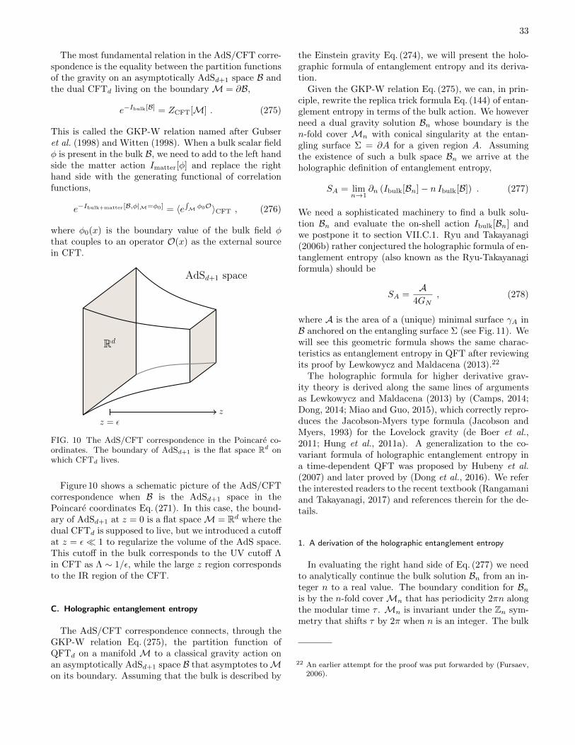
33

The most fundamental relation in the AdS/CFT corre-spondence is the equality between the partition functionsof the gravity on an asymptotically AdSd+1 space B andthe dual CFTd living on the boundary M = ∂B,

e−Ibulk[B] = ZCFT[M] . (275)

This is called the GKP-W relation named after Gubseret al. (1998) and Witten (1998). When a bulk scalar fieldφ is present in the bulk B, we need to add to the left handside the matter action Imatter[φ] and replace the righthand side with the generating functional of correlationfunctions,

e−Ibulk+matter[B,φ|M=φ0] = 〈e∫M φ0O〉CFT , (276)

where φ0(x) is the boundary value of the bulk field φthat couples to an operator O(x) as the external sourcein CFT.

AdSd+1 space

Rd

zz = ε

FIG. 10 The AdS/CFT correspondence in the Poincare co-ordinates. The boundary of AdSd+1 is the flat space Rd onwhich CFTd lives.

Figure 10 shows a schematic picture of the AdS/CFTcorrespondence when B is the AdSd+1 space in thePoincare coordinates Eq. (271). In this case, the bound-ary of AdSd+1 at z = 0 is a flat spaceM = Rd where thedual CFTd is supposed to live, but we introduced a cutoffat z = ε 1 to regularize the volume of the AdS space.This cutoff in the bulk corresponds to the UV cutoff Λin CFT as Λ ∼ 1/ε, while the large z region correspondsto the IR region of the CFT.

C. Holographic entanglement entropy

The AdS/CFT correspondence connects, through theGKP-W relation Eq. (275), the partition function ofQFTd on a manifold M to a classical gravity action onan asymptotically AdSd+1 space B that asymptotes toMon its boundary. Assuming that the bulk is described by

the Einstein gravity Eq. (274), we will present the holo-graphic formula of entanglement entropy and its deriva-tion.

Given the GKP-W relation Eq. (275), we can, in prin-ciple, rewrite the replica trick formula Eq. (144) of entan-glement entropy in terms of the bulk action. We howeverneed a dual gravity solution Bn whose boundary is then-fold cover Mn with conical singularity at the entan-gling surface Σ = ∂A for a given region A. Assumingthe existence of such a bulk space Bn we arrive at theholographic definition of entanglement entropy,

SA = limn→1

∂n (Ibulk[Bn]− n Ibulk[B]) . (277)

We need a sophisticated machinery to find a bulk solu-tion Bn and evaluate the on-shell action Ibulk[Bn] andwe postpone it to section VII.C.1. Ryu and Takayanagi(2006b) rather conjectured the holographic formula of en-tanglement entropy (also known as the Ryu-Takayanagiformula) should be

SA =A

4GN, (278)

where A is the area of a (unique) minimal surface γA inB anchored on the entangling surface Σ (see Fig. 11). Wewill see this geometric formula shows the same charac-teristics as entanglement entropy in QFT after reviewingits proof by Lewkowycz and Maldacena (2013).22

The holographic formula for higher derivative grav-ity theory is derived along the same lines of argumentsas Lewkowycz and Maldacena (2013) by (Camps, 2014;Dong, 2014; Miao and Guo, 2015), which correctly repro-duces the Jacobson-Myers type formula (Jacobson andMyers, 1993) for the Lovelock gravity (de Boer et al.,2011; Hung et al., 2011a). A generalization to the co-variant formula of holographic entanglement entropy ina time-dependent QFT was proposed by Hubeny et al.(2007) and later proved by (Dong et al., 2016). We referthe interested readers to the recent textbook (Rangamaniand Takayanagi, 2017) and references therein for the de-tails.

1. A derivation of the holographic entanglement entropy

In evaluating the right hand side of Eq. (277) we needto analytically continue the bulk solution Bn from an in-teger n to a real value. The boundary condition for Bnis by the n-fold coverMn that has periodicity 2πn alongthe modular time τ . Mn is invariant under the Zn sym-metry that shifts τ by 2π when n is an integer. The bulk

22 An earlier attempt for the proof was put forwarded by (Fursaev,2006).

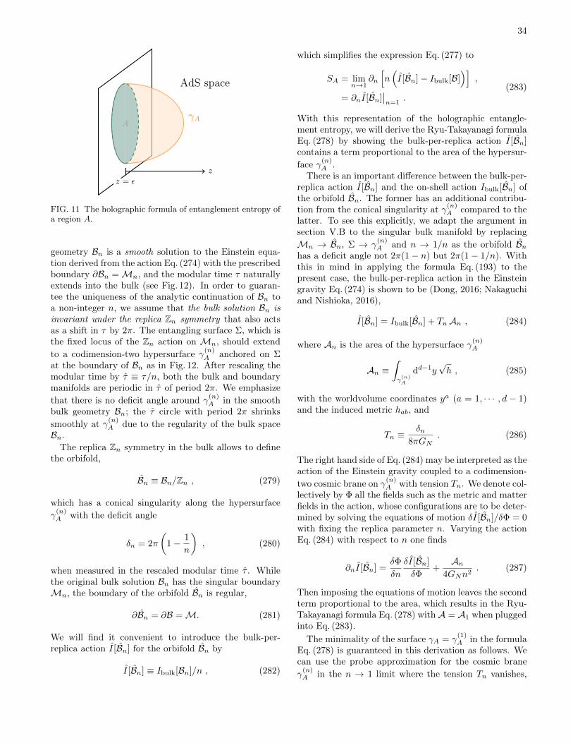
34

A

AdS space

z

z = ε

γA

FIG. 11 The holographic formula of entanglement entropy ofa region A.

geometry Bn is a smooth solution to the Einstein equa-tion derived from the action Eq. (274) with the prescribedboundary ∂Bn =Mn, and the modular time τ naturallyextends into the bulk (see Fig. 12). In order to guaran-tee the uniqueness of the analytic continuation of Bn toa non-integer n, we assume that the bulk solution Bn isinvariant under the replica Zn symmetry that also actsas a shift in τ by 2π. The entangling surface Σ, which isthe fixed locus of the Zn action on Mn, should extend

to a codimension-two hypersurface γ(n)A anchored on Σ

at the boundary of Bn as in Fig. 12. After rescaling themodular time by τ ≡ τ/n, both the bulk and boundarymanifolds are periodic in τ of period 2π. We emphasize

that there is no deficit angle around γ(n)A in the smooth

bulk geometry Bn; the τ circle with period 2π shrinks

smoothly at γ(n)A due to the regularity of the bulk space

Bn.

The replica Zn symmetry in the bulk allows to definethe orbifold,

Bn ≡ Bn/Zn , (279)

which has a conical singularity along the hypersurface

γ(n)A with the deficit angle

δn = 2π

(1− 1

n

), (280)

when measured in the rescaled modular time τ . Whilethe original bulk solution Bn has the singular boundaryMn, the boundary of the orbifold Bn is regular,

∂Bn = ∂B =M. (281)

We will find it convenient to introduce the bulk-per-replica action I[Bn] for the orbifold Bn by

I[Bn] ≡ Ibulk[Bn]/n , (282)

which simplifies the expression Eq. (277) to

SA = limn→1

∂n

[n(I[Bn]− Ibulk[B]

)],

= ∂nI[Bn]∣∣n=1

.(283)

With this representation of the holographic entangle-ment entropy, we will derive the Ryu-Takayanagi formulaEq. (278) by showing the bulk-per-replica action I[Bn]contains a term proportional to the area of the hypersur-

face γ(n)A .

There is an important difference between the bulk-per-replica action I[Bn] and the on-shell action Ibulk[Bn] ofthe orbifold Bn. The former has an additional contribu-tion from the conical singularity at γ

(n)A compared to the

latter. To see this explicitly, we adapt the argument insection V.B to the singular bulk manifold by replacing

Mn → Bn, Σ → γ(n)A and n → 1/n as the orbifold Bn

has a deficit angle not 2π(1− n) but 2π(1− 1/n). Withthis in mind in applying the formula Eq. (193) to thepresent case, the bulk-per-replica action in the Einsteingravity Eq. (274) is shown to be (Dong, 2016; Nakaguchiand Nishioka, 2016),

I[Bn] = Ibulk[Bn] + TnAn , (284)

where An is the area of the hypersurface γ(n)A

An ≡∫γ(n)A

dd−1y√h , (285)

with the worldvolume coordinates ya (a = 1, · · · , d − 1)and the induced metric hab, and

Tn ≡δn

8πGN. (286)

The right hand side of Eq. (284) may be interpreted as theaction of the Einstein gravity coupled to a codimension-

two cosmic brane on γ(n)A with tension Tn. We denote col-

lectively by Φ all the fields such as the metric and matterfields in the action, whose configurations are to be deter-mined by solving the equations of motion δI[Bn]/δΦ = 0with fixing the replica parameter n. Varying the actionEq. (284) with respect to n one finds

∂nI[Bn] =δΦ

δn

δI[Bn]

δΦ+An

4GNn2. (287)

Then imposing the equations of motion leaves the secondterm proportional to the area, which results in the Ryu-Takayanagi formula Eq. (278) withA = A1 when pluggedinto Eq. (283).

The minimality of the surface γA = γ(1)A in the formula

Eq. (278) is guaranteed in this derivation as follows. Wecan use the probe approximation for the cosmic brane

γ(n)A in the n → 1 limit where the tension Tn vanishes,

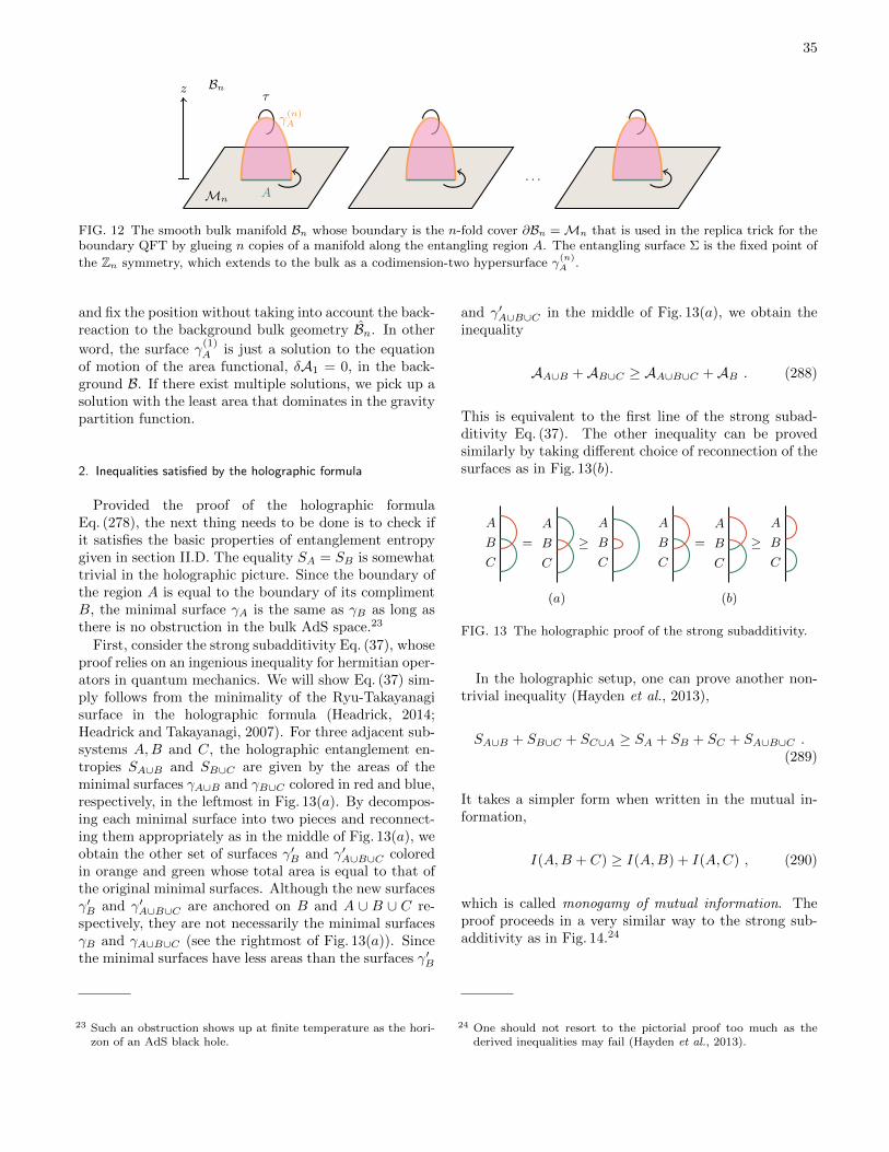
35

z

Mn

Bn

γ(n)A

A

τ

· · ·

FIG. 12 The smooth bulk manifold Bn whose boundary is the n-fold cover ∂Bn =Mn that is used in the replica trick for theboundary QFT by glueing n copies of a manifold along the entangling region A. The entangling surface Σ is the fixed point of

the Zn symmetry, which extends to the bulk as a codimension-two hypersurface γ(n)A .

and fix the position without taking into account the back-reaction to the background bulk geometry Bn. In other

word, the surface γ(1)A is just a solution to the equation

of motion of the area functional, δA1 = 0, in the back-ground B. If there exist multiple solutions, we pick up asolution with the least area that dominates in the gravitypartition function.

2. Inequalities satisfied by the holographic formula

Provided the proof of the holographic formulaEq. (278), the next thing needs to be done is to check ifit satisfies the basic properties of entanglement entropygiven in section II.D. The equality SA = SB is somewhattrivial in the holographic picture. Since the boundary ofthe region A is equal to the boundary of its complimentB, the minimal surface γA is the same as γB as long asthere is no obstruction in the bulk AdS space.23

First, consider the strong subadditivity Eq. (37), whoseproof relies on an ingenious inequality for hermitian oper-ators in quantum mechanics. We will show Eq. (37) sim-ply follows from the minimality of the Ryu-Takayanagisurface in the holographic formula (Headrick, 2014;Headrick and Takayanagi, 2007). For three adjacent sub-systems A,B and C, the holographic entanglement en-tropies SA∪B and SB∪C are given by the areas of theminimal surfaces γA∪B and γB∪C colored in red and blue,respectively, in the leftmost in Fig. 13(a). By decompos-ing each minimal surface into two pieces and reconnect-ing them appropriately as in the middle of Fig. 13(a), weobtain the other set of surfaces γ′B and γ′A∪B∪C coloredin orange and green whose total area is equal to that ofthe original minimal surfaces. Although the new surfacesγ′B and γ′A∪B∪C are anchored on B and A ∪ B ∪ C re-spectively, they are not necessarily the minimal surfacesγB and γA∪B∪C (see the rightmost of Fig. 13(a)). Sincethe minimal surfaces have less areas than the surfaces γ′B

23 Such an obstruction shows up at finite temperature as the hori-zon of an AdS black hole.

and γ′A∪B∪C in the middle of Fig. 13(a), we obtain theinequality

AA∪B +AB∪C ≥ AA∪B∪C +AB . (288)

This is equivalent to the first line of the strong subad-ditivity Eq. (37). The other inequality can be provedsimilarly by taking different choice of reconnection of thesurfaces as in Fig. 13(b).

A

B

C

=

A

B

C

(a)

≥A

B

C

A

B

C

=

A

B

C

(b)

≥A

B

C

FIG. 13 The holographic proof of the strong subadditivity.

In the holographic setup, one can prove another non-trivial inequality (Hayden et al., 2013),

SA∪B + SB∪C + SC∪A ≥ SA + SB + SC + SA∪B∪C .(289)

It takes a simpler form when written in the mutual in-formation,

I(A,B + C) ≥ I(A,B) + I(A,C) , (290)

which is called monogamy of mutual information. Theproof proceeds in a very similar way to the strong sub-additivity as in Fig. 14.24

24 One should not resort to the pictorial proof too much as thederived inequalities may fail (Hayden et al., 2013).

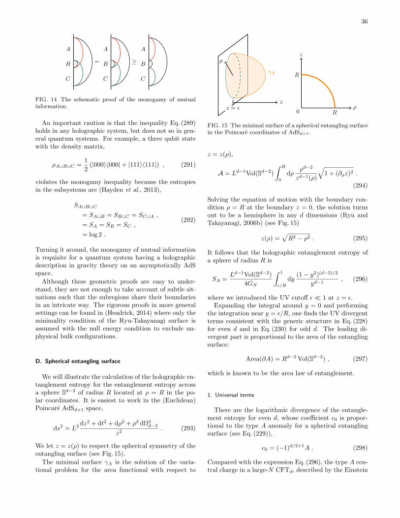
36

A

B

C

=

A

B

C

≥

A

B

C

FIG. 14 The schematic proof of the monogamy of mutualinformation.

An important caution is that the inequality Eq. (289)holds in any holographic system, but does not so in gen-eral quantum systems. For example, a three qubit statewith the density matrix,

ρA∪B∪C =1

2(|000〉〈000|+ |111〉〈111|) , (291)

violates the monogamy inequality because the entropiesin the subsystems are (Hayden et al., 2013),

SA∪B∪C

= SA∪B = SB∪C = SC∪A ,

= SA = SB = SC ,

= log 2 .

(292)

Turning it around, the monogamy of mutual informationis requisite for a quantum system having a holographicdescription in gravity theory on an asymptotically AdSspace.

Although these geometric proofs are easy to under-stand, they are not enough to take account of subtle sit-uations such that the subregions share their boundariesin an intricate way. The rigorous proofs in more generalsettings can be found in (Headrick, 2014) where only theminimality condition of the Ryu-Takayanagi surface isassumed with the null energy condition to exclude un-physical bulk configurations.

D. Spherical entangling surface

We will illustrate the calculation of the holographic en-tanglement entropy for the entanglement entropy acrossa sphere Sd−2 of radius R located at ρ = R in the po-lar coordinates. It is easiest to work in the (Euclidean)Poincare AdSd+1 space,

ds2 = L2 dz2 + dt2 + dρ2 + ρ2 dΩ2d−2

z2. (293)

We let z = z(ρ) to respect the spherical symmetry of theentangling surface (see Fig. 15).

The minimal surface γA is the solution of the varia-tional problem for the area functional with respect to

ρ

zz = ε

γA

ρ

z

R

R

0

FIG. 15 The minimal surface of a spherical entangling surfacein the Poincare coordinates of AdSd+1.

z = z(ρ),

A = Ld−1Vol(Sd−2)

∫ R

0

dρρd−2

zd−1(ρ)

√1 + (∂ρz)2 .

(294)

Solving the equation of motion with the boundary con-dition ρ = R at the boundary z = 0, the solution turnsout to be a hemisphere in any d dimensions (Ryu andTakayanagi, 2006b) (see Fig. 15)

z(ρ) =√R2 − ρ2 . (295)

It follows that the holographic entanglement entropy ofa sphere of radius R is

SA =Ld−1Vol(Sd−2)

4GN

∫ 1

ε/R

dy(1− y2)(d−3)/2

yd−1, (296)

where we introduced the UV cutoff ε 1 at z = ε.Expanding the integral around y = 0 and performing

the integration near y = ε/R, one finds the UV divergentterms consistent with the generic structure in Eq. (228)for even d and in Eq. (230) for odd d. The leading di-vergent part is proportional to the area of the entanglingsurface:

Area(∂A) = Rd−2 Vol(Sd−2) , (297)

which is known to be the area law of entanglement.

1. Universal terms

There are the logarithmic divergence of the entangle-ment entropy for even d, whose coefficient c0 is propor-tional to the type A anomaly for a spherical entanglingsurface (see Eq. (229)),

c0 = (−1)d/2+1A . (298)

Compared with the expression Eq. (296), the type A cen-tral charge in a large-N CFTd, described by the Einstein

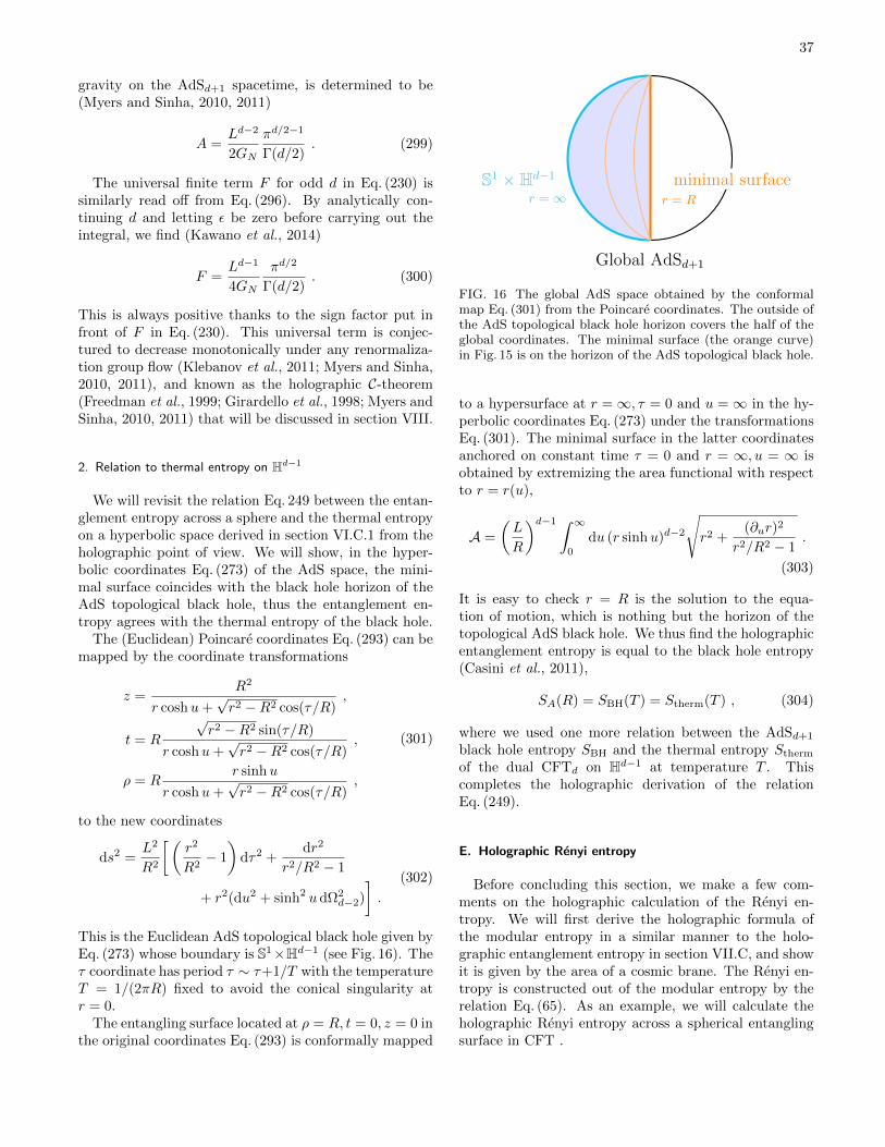
37

gravity on the AdSd+1 spacetime, is determined to be(Myers and Sinha, 2010, 2011)

A =Ld−2

2GN

πd/2−1

Γ(d/2). (299)

The universal finite term F for odd d in Eq. (230) issimilarly read off from Eq. (296). By analytically con-tinuing d and letting ε be zero before carrying out theintegral, we find (Kawano et al., 2014)

F =Ld−1

4GN

πd/2

Γ(d/2). (300)

This is always positive thanks to the sign factor put infront of F in Eq. (230). This universal term is conjec-tured to decrease monotonically under any renormaliza-tion group flow (Klebanov et al., 2011; Myers and Sinha,2010, 2011), and known as the holographic C-theorem(Freedman et al., 1999; Girardello et al., 1998; Myers andSinha, 2010, 2011) that will be discussed in section VIII.

2. Relation to thermal entropy on Hd−1

We will revisit the relation Eq. 249 between the entan-glement entropy across a sphere and the thermal entropyon a hyperbolic space derived in section VI.C.1 from theholographic point of view. We will show, in the hyper-bolic coordinates Eq. (273) of the AdS space, the mini-mal surface coincides with the black hole horizon of theAdS topological black hole, thus the entanglement en-tropy agrees with the thermal entropy of the black hole.

The (Euclidean) Poincare coordinates Eq. (293) can bemapped by the coordinate transformations

z =R2

r coshu+√r2 −R2 cos(τ/R)

,

t = R

√r2 −R2 sin(τ/R)

r coshu+√r2 −R2 cos(τ/R)

,

ρ = Rr sinhu

r coshu+√r2 −R2 cos(τ/R)

,

(301)

to the new coordinates

ds2 =L2

R2

[(r2

R2− 1

)dτ2 +

dr2

r2/R2 − 1

+ r2(du2 + sinh2 udΩ2d−2)

].

(302)

This is the Euclidean AdS topological black hole given byEq. (273) whose boundary is S1×Hd−1 (see Fig. 16). Theτ coordinate has period τ ∼ τ+1/T with the temperatureT = 1/(2πR) fixed to avoid the conical singularity atr = 0.

The entangling surface located at ρ = R, t = 0, z = 0 inthe original coordinates Eq. (293) is conformally mapped

r = R

minimal surfacer =∞

S1 ×Hd−1

Global AdSd+1

FIG. 16 The global AdS space obtained by the conformalmap Eq. (301) from the Poincare coordinates. The outside ofthe AdS topological black hole horizon covers the half of theglobal coordinates. The minimal surface (the orange curve)in Fig. 15 is on the horizon of the AdS topological black hole.

to a hypersurface at r =∞, τ = 0 and u =∞ in the hy-perbolic coordinates Eq. (273) under the transformationsEq. (301). The minimal surface in the latter coordinatesanchored on constant time τ = 0 and r = ∞, u = ∞ isobtained by extremizing the area functional with respectto r = r(u),

A =

(L

R

)d−1 ∫ ∞0

du (r sinhu)d−2

√r2 +

(∂ur)2

r2/R2 − 1.

(303)

It is easy to check r = R is the solution to the equa-tion of motion, which is nothing but the horizon of thetopological AdS black hole. We thus find the holographicentanglement entropy is equal to the black hole entropy(Casini et al., 2011),

SA(R) = SBH(T ) = Stherm(T ) , (304)

where we used one more relation between the AdSd+1

black hole entropy SBH and the thermal entropy Stherm

of the dual CFTd on Hd−1 at temperature T . Thiscompletes the holographic derivation of the relationEq. (249).

E. Holographic Renyi entropy

Before concluding this section, we make a few com-ments on the holographic calculation of the Renyi en-tropy. We will first derive the holographic formula ofthe modular entropy in a similar manner to the holo-graphic entanglement entropy in section VII.C, and showit is given by the area of a cosmic brane. The Renyi en-tropy is constructed out of the modular entropy by therelation Eq. (65). As an example, we will calculate theholographic Renyi entropy across a spherical entanglingsurface in CFT .

38

1. A derivation of the holographic formula

The argument for deriving the Ryu-Takayanagi for-mula in section VII.C.1 has more implications for theholographic description of quantum entanglement than itappears. The modular entropy Eq. (62) written in termsof the partition function

Sn = (1− n∂n)(logZn − n logZ) , (305)

can be turned, with the GKP-W relation and the bulk-per-replica action Eq. (282), into the neat form,

Sn = (n∂n − 1)[n(I[Bn]− Ibulk[B])

],

= n2∂nI[Bn] .(306)

This reminds us of the holographic definition of entangle-ment entropy Eq. (283), and one can recycle the resultingrelation Eq. (287) to find the holographic formula of themodular entropy (Dong, 2016),

Sn =An

4GN

∣∣∣∣δI=0, ∂γ

(n)A =Σ

. (307)

It resembles to the Ryu-Takayanagi formula Eq. (278)and actually reproduces it when n = 1. This formula,however, contains the area of a codimension-two cos-

mic brane γ(n)A with tension Tn given by Eq. (286) that

backreacts to the bulk geometry. Hence it is more in-tricate in practice than the case of the Ryu-Takayanagiformula Eq. (278) as we have to fix the location of thecosmic brane by solving the equations of motion of theaction I describing the Einstein gravity coupled to thecosmic brane and possibly matter fields as indicatedby the subscript δI = 0 in the formula Eq. (307) (seeEq. (287) for the definition of I). We are also able tobulid the holographic Renyi entropy by combining theformula Eq. (307) with the relation Eq. (65).

Given the holographic formula of the Renyi entropy,one may ask whether it satisfies the inequalities Eq. (56)-(59) characterizing the Renyi entropy. To this end it isenough to check the three inequalities Eq. (63) implyingthe non-negativities of the modular energy, entropy andcapacity. The easiest one to show is the inequality Sn ≥ 0that follows from the non-negativity of the area of a cos-mic brane in the formula Eq. (307). The non-negativityof the modular energy E ≥ 0 becomes clear by expressingE in the form,

E = Ibulk[Bn]− Ibulk[B] +An

4GN, (308)

and invoking B be the on-shell solution with the leastaction while Bn is not necessarily so. The last inequal-ity C ≥ 0 for the modular capacity is most non-trivial,and turns out to require the stability of the bulk geom-etry Bn (Nakaguchi and Nishioka, 2016). It remains anopen issue whether and when such a stability conditionis guaranteed to hold in the holographic setup.

2. Spherical entangling surface in CFT

We have seen in section VII.D.2 that the entanglemententropy across a spherical entangling surface in CFT isequal to the thermal entropy on Hd−1 at inverse temper-ature 2πR, and can be calculated holographically as theblack hole entropy in the dual AdS spacetime. Here wewill see the holographic formula of the modular entropy(307) also has an elegant interpretation as a black holeentropy when the entangling surface is spherical in accor-dance with the CFT story in section VI.C (Hung et al.,2011b).

The AdS topological black hole given by Eq. (302) is aparticular case of the following AdS black hole,

ds2 =L2

R2

[f(r) dτ2 +

dr2

f(r)+ r2(du2 + sinh2 udΩ2

d−2)

].

(309)

where the function f(r) vanishes at r = rH ,

f(r) =r2

R2− 1−

rd−2H

rd−2

(r2H

R2− 1

). (310)

This black hole has a temperature parametrized by adimensionless parameter x ≡ rH/R,

T (x) =1

4πR

[d x− d− 2

x

], (311)

and the dual CFT lives on the boundary that is a hyper-bolic space Hd−1 at finite temperature T (x).

In this setup, the codimension-two cosmic brane in theformula (307) is at the black hole horizon and the mod-ular entropy can be identified with the thermal entropyby matching the black hole temperature Eq. (311) withTn = 1/(2πRn). By setting x to be

xn =1 +

√dn2(d− 2) + 1

dn, (312)

the black hole entropy at temperature Tn becomes

Sn = Stherm (Tn) =Vol(Hd−1)Ld−1

4GNxd−1n . (313)

Performing the integration in Eq. (65) or Eq. (248) leadsto the Renyi entropy,

Sn =Vol(Hd−1)Ld−1

4GN

n

2(n− 1)

(2− xd−2

n − xdn).

(314)

VIII. RENORMALIZATION GROUP FLOWS

In this section, we turn our attention to the dynam-ical aspects of entanglement entropy under a renormal-ization group (RG) flow. We first overview the idea of

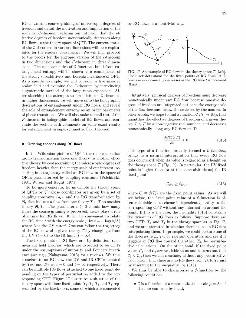
39

RG flows as a course-graining of microscopic degrees offreedom and detail the motivation and implication of theso-called C-theorem realizing our intuition that the ef-fective degrees of freedom monotonically decreases alongRG flows in the theory space of QFT. The current statusof the C-theorems in various dimensions will be recapitu-lated for the readers’ convenience. We will then proceedto the proofs for the entropic version of the c-theoremin two dimensions and the F -theorem in three dimen-sions. The monotonicities of C-functions build from en-tanglement entropy will be shown as a consequence ofthe strong subadditivity and Lorentz invariance of QFT.As a specific example, we will consider a free massivescalar field and examine the F -theorem by introducinga systematic method of the large mass expansion. Af-ter sketching the attempts to formulate the C-theoremsin higher dimensions, we will move onto the holographicdescriptions of entanglement under RG flows, and revealthe role of entanglement entropy as an order parameterof phase transitions. We will also make a small test of theF -theorem in holographic models of RG flows, and con-clude the section with comments on some exact resultsfor entanglement in supersymmetric field theories.

A. Ordering theories along RG flows

In the Wilsonian picture of QFT, the renormalizationgroup transformation takes one theory to another effec-tive theory by coarse-graining the microscopic degrees offreedom heavier than the energy scale of our interest, re-sulting in a trajectory called an RG flow in the space ofQFTs parameterized by coupling constants (Polchinski,1984; Wilson and Kogut, 1974).

To be more concrete, let us denote the theory spaceof QFTs by T whose coordinates are given by a set ofcoupling constants gi, and the RG transformation byRt that induces a flow from one theory T ∈ T to anothertheory Rt T . The parameter t ≥ 0 counts how manytimes the coarse-graining is processed, hence plays a roleof a time for RG flows. It will be convenient to relatethe RG time t with the energy scale µ by t = − log(µ/Λ)where Λ is the UV cutoff. One can follow the trajectoryof the RG flow of a given theory T by changing t fromthe UV (t = 0) to the IR limit (t =∞).

The fixed points of RG flows are, by definition, scaleinvariant field theories, which are expected to be CFTsunder the assumptions of unitarity and Poincare invari-ance (see e.g., (Nakayama, 2015) for a review). We thusassociate to an RG flow the UV and IR CFTs denotedby TUV and TIR at t = 0 and t = ∞ respectively. Therecan be multiple RG flows attached to one fixed point de-pending on the types of perturbation added to the cor-responding CFT. Figure 17 illustrates a situation of thetheory space with four fixed points T1, T2, T3 and T4 rep-resented by the black dots, some of which are connected

by RG flows in a nontrivial way.

R

R′

R′′

?

?

T1

T3

T4

T2 t

C

C1

C2

FIG. 17 An example of RG flows in the theory space T [Left].The black dots stand for the fixed points of RG flows. A C-function monotonically decreases as the RG time t is increased[Right].

Intuitively, physical degrees of freedom must decreasemonotonically under any RG flow because massive de-grees of freedom are integrated out once the energy scaleof the flow becomes below the scale set by the masses. Inother words, we hope to find a function C : T → R≥0 thatquantifies the effective degrees of freedom of a given the-ory T ∈ T by a non-negative real number, and decreasesmonotonically along any RG flow on T :

d C(Rt T )

dt≤ 0 . (315)

This type of a function, broadly termed a C-function,brings us a natural interpretation that every RG flowgoes downward when its value is regarded as a height onthe theory space T (Fig. 17). In particular, the UV fixedpoint is higher than (or at the same altitude as) the IRfixed point:

CUV ≥ CIR , (316)

where Ci ≡ C(Ti) are the fixed point values. As we willsee below, the fixed point value of a C-function is of-ten calculable as a scheme-independent quantity in thecorresponding CFT without any information around thepoint. If this is the case, the inequality (316) constrainsthe dynamics of RG flows as follows. Suppose there aretwo CFTs T3 and T4 in the theory space as in Fig. 17,and we are interested in whether there exists an RG flowinterpolating them. In principle, we could perturb one ofthe theories, e.g., T3, by relevant operators and see if ittriggers an RG flow toward the other, T4, by perturba-tive calculations. On the other hand, if the fixed pointvalues C3 and C4 are available to us and it turns out thatC3 < C4, then we can conclude, without any perturbativecalculation, that there are no RG flows from T3 to T4 justby resorting to the inequality Eq. (316).

We thus be able to characterize a C-function by thefollowing conditions:

• C is a function of a renormalization scale µ = Λ e−t

that we can tune by hand,

40

• C is well-defined for any QFT, independent of thetypes of field contents and their interactions,

• C is a monotonic function of the renormalizationtime t for any unitary and Lorentz invariant QFTin one of the following senses (Barnes et al., 2004;Gukov, 2016):

(i) [Weak version] The fixed point value of Cshould decrease along RG flows as in Eq.(316).

(ii) [Stronger version] C monotonically decreasesalong the entire RG flow as in Eq. (315).

(iii) [Strongest version] C is a potential that gener-ates RG flows:

βi(g) = Gij(g)∂C∂gj

, (317)

where βi(g) ≡ −dgi/dt and Gij(g) is apositive-definite metric on the theory space T .

Here we distinguish the three versions of a C-functionin increasing order of strength for completeness. Theweak version follows from the stronger one by integratingEq. (315) along the flow. The stronger version is impliedby the strongest one too,

d Cdt

= −βi∂ C∂gi

= −Gij∂ C∂gi

∂ C∂gj≤ 0 . (318)

While the existence of a C-function may be taken forgranted from the physical point of view, the problem ishow to construct such a well-behaved function satisfyingthe aforementioned properties. Indeed the constructionof a C-function for QFT in dimensions higher than twohas been a long-standing problem for three decades sincethe initiating work by Zamolodchikov (1986), and wassuccessfully settled down quite recently in only three andfour dimensions.

One possible approach to this problem is to formulate aset of axioms that guarantee the existence of a C-functionin any dimension without any explicit construction. Thepower of an axiomatic approach is well demonstratedin (axiomatic) thermodynamics whose most importantconsequence is the very existence of a (unique) entropyfunction that never decreases under adiabatic processesand characterizes thermal equilibrium states when repre-sented as a function of extensive variables such as energyand volume (see e.g., (Lieb and Yngvason, 1999) for anexcellent reference on the subject). In fact, there are con-siderable similarities between the theory space of QFTand the state space of thermodynamics. For instance,the irreversibility of an RG flow between two fixed pointsTa, Tb ∈ T corresponds to an irreversible adiabatic pro-cess a→ b that takes one equilibrium state a to the otherb. A partial list of the analogies between thermodynam-ics and QFT is shown in Table IV. It would be of great

TABLE IV An analogy between thermodynamics and QFT.

Thermodynamics QFTEquilibrium states Conformal fixed points

a, b Ta, TbUnion of two states Coupling of two theories

a+ b Ta and TbIrreversible adiabatic process RG flow

a→ b from Ta to TbEntropy function C-function

interest to translate the set of axioms for equilibriumthermodynamics into the language of QFT, and examineto what extent the formulation of an entropy functioncarries over to the construction of a C-function. We shallnot address this possibility any further in this article andleave it to future investigations. Instead, we will take aconstructive approach for a C-function in the subsequentsubsections.

B. List of C-theorems

We pause to sketch a list of the known C-theoremsand related conjectures in various dimensions, with briefcomments on their historical backgrounds.

1. Two dimensions

In 1986, Zamolodchikov (1986) proved his celebratedc-theorem in the following form.

Theorem (Zamolodchikov’s c-theorem). In two-dimensional renormalizable QFTs, there exists theZamolodchikov’s c-function c(gi, µ) that depends on a setof dimensionless coupling constants gi and the energyscale µ(= Λ e−t), satisfying the following properties:

1. it takes the same value as the central charge c ofthe CFT corresponding to each fixed point of RGflows:

c(gi, µ)|CFT = c , (319)

2. it monotonically decreases along any RG flow:

d c(gi, µ)

dt= −µd c(gi, µ)

dµ≤ 0 , (320)

3. it is stationary only at the fixed points:

∂ c(gi, µ)

∂gi

∣∣∣∣CFT

= 0 . (321)

Hence, Zamolodchikov’s c-theorem falls into thestrongest version in the terminology introduced in the

41

previous subsection (see also (Friedan and Konechny,2010)). The Zamolodchikov’s c-function can be build ex-plicitly from the two-point correlation functions of thestress-energy tensor in two dimensions, and the mono-tonicity follows from the reflection positivity of the cor-relator.

2. Three dimensions

Given the fact that the Zamolodchikov’s c-functiongives the central charge at the fixed points, it is temptingto look for counterparts of the two-dimensional centralcharge in d > 2 dimensions. Let us consider a few candi-dates for central charges that can be defined irrespectiveof dimensionality:

(a) A “thermal central charge” CTherm as a coefficientof the thermal free energy density fTherm at finitetemperature T defined by

fTherm ∼ CTherm T d . (322)

(b) The coefficient CT for the two-point function of thestress-energy tensor in Eq. (216).

(c) The central charges A, Bi for the conformal anoma-lies defined by Eq. (210) that exist only in even ddimensions.

In d = 2 dimensions, all of these are known to be pro-portional to the central charge, CTherm ∝ CT ∝ A ∝ c,for CFT, but they do not generally have linear relationsin higher dimensions.

The possibility (a) of adopting the thermal centralcharge CTherm as a measure of degrees of freedom wasstudied by Sachdev (1993) for the three-dimensionalO(N) vector model in the large-N limit. This model hasthe RG flow from the Gaussian fixed point, TGaussian,where all the N scalar fields are free and massless, to thecritical O(N) (interacting) fixed point, Tcritical, by keep-ing the renormalized masses vanishing. Perturbing thecritical O(N) fixed point by giving the scalars negativemass squared terms triggers the RG flow to the O(N−1)symmetric (Goldstone) fixed point, TGoldstone, with N−1massless free scalar fields (Goldstone modes).25 If thethermal central charge measures the degrees of free-dom correctly, we expect them to be ordered alongthe RG flow, CTherm(TGaussian) > CTherm(Tcritical) >CTherm(TGoldstone). The thermal central charges atthe Gaussian and Goldstone fixed points are simplygiven by CTherm(TGaussian) = N CTherm(Tscalar) and

25 There is one massive scalar field that decouples at the Goldstonefixed point.

CTherm(TGoldstone) = (N − 1)CTherm(Tscalar) as con-sistent with the RG flow, where Tscalar is a realmassless free scalar field theory. On the otherhand, the large-N analysis showed CTherm(Tcritical) =(4N/5 +O(1)) CTherm(Tscalar), which can be less thanthe IR value, CTherm(TGoldstone), for large N , and ruledout the possibility of CTherm being the fixed point valueof a C-function (Sachdev, 1993).

The option (b) employing the coefficient CT as afixed point value of a C-function was suggested in(Petkou, 1995) based on the result CT (Tcritical) =(N − 40/(9π2)

)CT (Tscalar) consistent with the RG flows

described above for the O(N) vector model. This pos-sibility was explored in (Nishioka and Yonekura, 2013)more systematically for N = 2 supersymmetric field the-ories in three dimensions that allows the exact calculationof CT due to the supersymmetric localization technique.In that work, it was shown that a supersymmetric ana-logue of the O(N) vector model (N = 2 Wess-Zuminomodel) can be a counterexample for the “CT ”-theorem.Another counterexample was also found in (Fei et al.,2014) by examining the RG flows in the five-dimensionalO(N) symmetric scalar field theory with the O(N) sym-metric interacting fixed point.

In three dimensions, there exists no conformalanomaly, hence the third option (c) is unavailable in itsown. Alternatively, an ingenious proposal was made byJafferis et al. (2011) (and independently by Myers andSinha (2010, 2011) in a different form from the holo-graphic viewpoint) based on the extremization principleof the supersymmetric partition function (Jafferis, 2010),which is now known as the F -theorem,

Theorem (F -theorem). In three-dimensional QFTs,there exists a function F(gi, µ) on the theory space satis-fying the following properties:

1. it takes the same value as the sphere free energy Fof the CFT corresponding to each fixed point of RGflows,

F(gi, µ)|CFT = F , (323)

where F = − log |Z[S3]| and Z[S3] is the (renor-malized) Euclidean partition function on S3,

2. it is a monotonically decreasing function under anyRG flow,

dFd t

= −µdFdµ≤ 0 . (324)

This statement can be regarded as a variant of thethird option (c) since we can extract the type A centralcharge of the conformal anomaly from the sphere parti-tion function, A ∝ logZ[Sd] in even dimensions.

While the F -theorem was originally stated in the weakform, FUV ≥ FIR, a perturbative argument (Klebanov

42

et al., 2011; Yonekura, 2013) suggests the sphere free en-ergy is a strongest version of a C-function. A strong evi-dence supporting the F -theorem was given for N = 2 su-persymmetric theories with U(1)R symmetry, where thesphere free energy F is shown to be locally maximizedat RG fixed points (Closset et al., 2012; Jafferis, 2010)unless there is no accidental symmetry at the IR fixedpoint (see also the review (Pufu, 2016) for details). Anon-perturbative proof of the strong version of the F -theorem stated above is given Casini and Huerta (2012)by exploiting the unexpected relation between the freeenergy and the entanglement entropy of a disk we de-rived in Eq. (255). We will outline the insightful proofand the implications in section VIII.D.

3. Four dimensions

Seeking for a C-theorem in four dimensions has a longhistory starting from the conjecture (of the type (c) insection VIII.A) by Cardy (1988) for the a-theorem,

Theorem (a-theorem). In four-dimensional QFTs, thethe type A central charge a of the conformal anomalydecreases along any RG flow,

aUV ≥ aIR . (325)

This weak version of the a-theorem has passed a num-ber of tests over the years in perturbative QFTs (Jackand Osborn, 1990; Osborn, 1989), and was given an ev-idence for N = 1 supersymmetric theories by the a-maximization method that implies a strongest a-theorem(Barnes et al., 2004; Intriligator and Wecht, 2003). Aproof of the a-theorem without relying on supersymme-try was presented more recently by Komargodski andSchwimmer (2011) who connect the difference of the a-coefficient with the scattering amplitude of four dilatonfields that naturally couple to the stress-energy tensor(see also (Komargodski, 2012)). Interestingly the unitar-ity of the scattering amplitude turns out to guarantee theinequality (325) in their proof.

Recently, an alternative proof of the a-theorem wasgiven by Casini et al. (2017a) who resort to the mono-tonicity of entanglement as in the case of the F -theorem.We will touch on the proof in section VIII.E.

Finally, a few comments on the other possibilities arein order:

(a) The thermal central charge CTherm does not satisfya C-theorem in a class of four-dimensional gaugetheories that are not asymptotically free at UV(Appelquist et al., 1999).

(b, c) The CT coefficient of the stress tensor two-pointfunction is proportional to the type B centralcharge c, CT ∝ c, in four dimensions (Os-born and Petkou, 1994). The latter has been

extensively studied in supersymmetric and non-supersymmetric theories and many counterexam-ples are known in a typical class of gauge theories(Anselmi et al., 1998; Cappelli et al., 1991).

4. Higher dimensions

Given the success in d ≤ 4 dimensions, one may betempted to extend a C-theorem to higher dimensions,d > 4. This problem is less explored than the lower-dimensional cases, but once formulated, it will provideus a unifying picture of RG flows in QFT irrespectiveof dimensionality. It should be too early to survey thewhole subject as it is still under active investigation. Wethus only comment on two promising conjectures:26

• The a-theorem in higher even dimensions postu-lates the monotonicity of the type A central chargefor the conformal anomaly under RG flows. Thereare supporting evidences for the a-theorem fromholography (Myers and Sinha, 2010, 2011) and evenproofs for a certain class of supersymmetric fieldtheories in six dimensions (Cordova et al., 2016,2015).

• The F -theorem in higher odd dimensions is sug-gested by (Klebanov et al., 2011; Myers and Sinha,2010, 2011) and further incorporated into the gen-eralized F -theorem proposal Giombi and Klebanov(2015) that interpolates between the F -theoremand the a-theorem in non-integer dimensions. Afew examples supporting the F -theorem in five di-mensions are presented in (Fei et al., 2014; Jafferisand Pufu, 2014).

C. The entropic c-theorem in (1 + 1) dimensions

We shall prove (the strong version of) the C-theoremin two dimensions by constructing a C-function buildfrom entanglement entropy. A C-function should be well-defined for any QFT and monotonically decreases as theenergy scale µ is lowered while fixing the size of a system(e.g., an entangling region). One good candidate for it isthe entanglement entropy S(R) of an interval of width Rin (1 + 1) dimensions (see Fig. 18).

Rx

FIG. 18 An interval of width R as an entangling region.

26 See also (Gukov, 2016, 2017) for a recent discussion on constrain-ing RG flows by topological data of the theory space.

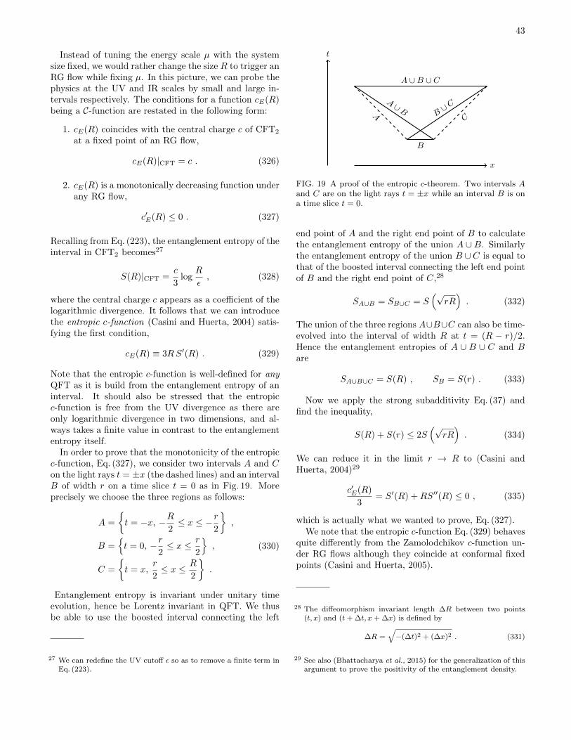
43

Instead of tuning the energy scale µ with the systemsize fixed, we would rather change the size R to trigger anRG flow while fixing µ. In this picture, we can probe thephysics at the UV and IR scales by small and large in-tervals respectively. The conditions for a function cE(R)being a C-function are restated in the following form:

1. cE(R) coincides with the central charge c of CFT2

at a fixed point of an RG flow,

cE(R)|CFT = c . (326)

2. cE(R) is a monotonically decreasing function underany RG flow,

c′E(R) ≤ 0 . (327)

Recalling from Eq. (223), the entanglement entropy of theinterval in CFT2 becomes27

S(R)|CFT =c

3log

R

ε, (328)

where the central charge c appears as a coefficient of thelogarithmic divergence. It follows that we can introducethe entropic c-function (Casini and Huerta, 2004) satis-fying the first condition,

cE(R) ≡ 3RS′(R) . (329)

Note that the entropic c-function is well-defined for anyQFT as it is build from the entanglement entropy of aninterval. It should also be stressed that the entropicc-function is free from the UV divergence as there areonly logarithmic divergence in two dimensions, and al-ways takes a finite value in contrast to the entanglemententropy itself.

In order to prove that the monotonicity of the entropicc-function, Eq. (327), we consider two intervals A and Con the light rays t = ±x (the dashed lines) and an intervalB of width r on a time slice t = 0 as in Fig. 19. Moreprecisely we choose the three regions as follows:

A =

t = −x, −R

2≤ x ≤ −r

2

,

B =t = 0, −r

2≤ x ≤ r

2

,

C =

t = x,

r

2≤ x ≤ R

2

.

(330)

Entanglement entropy is invariant under unitary timeevolution, hence be Lorentz invariant in QFT. We thusbe able to use the boosted interval connecting the left

27 We can redefine the UV cutoff ε so as to remove a finite term inEq. (223).

x

t

B

A ∪B ∪ C

AC

B∪ C

A ∪B

FIG. 19 A proof of the entropic c-theorem. Two intervals Aand C are on the light rays t = ±x while an interval B is ona time slice t = 0.

end point of A and the right end point of B to calculatethe entanglement entropy of the union A ∪ B. Similarlythe entanglement entropy of the union B ∪C is equal tothat of the boosted interval connecting the left end pointof B and the right end point of C,28

SA∪B = SB∪C = S(√

rR). (332)

The union of the three regions A∪B∪C can also be time-evolved into the interval of width R at t = (R − r)/2.Hence the entanglement entropies of A ∪ B ∪ C and Bare

SA∪B∪C = S(R) , SB = S(r) . (333)

Now we apply the strong subadditivity Eq. (37) andfind the inequality,

S(R) + S(r) ≤ 2S(√

rR). (334)

We can reduce it in the limit r → R to (Casini andHuerta, 2004)29

c′E(R)

3= S′(R) +RS′′(R) ≤ 0 , (335)

which is actually what we wanted to prove, Eq. (327).We note that the entropic c-function Eq. (329) behaves

quite differently from the Zamolodchikov c-function un-der RG flows although they coincide at conformal fixedpoints (Casini and Huerta, 2005).

28 The diffeomorphism invariant length ∆R between two points(t, x) and (t+ ∆t, x+ ∆x) is defined by

∆R =√−(∆t)2 + (∆x)2 . (331)

29 See also (Bhattacharya et al., 2015) for the generalization of thisargument to prove the positivity of the entanglement density.

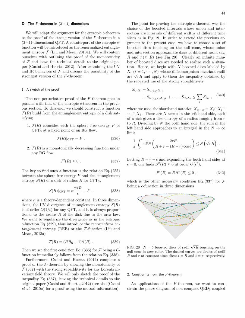
44

D. The F -theorem in (2 + 1) dimensions

We will adapt the argument for the entropic c-theoremto the proof of the strong version of the F -theorem in a(2+1)-dimensional QFT. A counterpart of the entropic c-function will be introduced as the renormalized entangle-ment entropy F (Liu and Mezei, 2013a). We will contentourselves with outlining the proof of the monotonicityof F and leave the technical details to the original pa-per (Casini and Huerta, 2012). After examining the UVand IR behaviors of F and discuss the possibility of thestrongest version of the F -theorem.

1. A sketch of the proof

The non-perturbative proof of the F -theorem goes inparallel with that of the entropic c-theorem in the previ-ous section. To this end, we should construct a functionF(R) build from the entanglement entropy of a disk sat-isfying

1. F(R) coincides with the sphere free energy F ofCFT3 at a fixed point of an RG flow,

F(R)|CFT = F . (336)

2. F(R) is a monotonically decreasing function underany RG flow,

F ′(R) ≤ 0 . (337)

The key to find such a function is the relation Eq. (255)between the sphere free energy F and the entanglemententropy S(R) of a disk of radius R for CFT3,

S(R)|CFT = α2πR

ε− F , (338)

where α is a theory-dependent constant. In three dimen-sions, the UV divergence of entanglement entropy S(R)is of order O(1/ε) for any QFT, and it is always propor-tional to the radius R of the disk due to the area law.We want to regularize the divergence as in the entropicc-function Eq. (329), thus introduce the renormalized en-tanglement entropy (REE) or the F-function (Liu andMezei, 2013a)

F(R) ≡ (R∂R − 1)S(R) . (339)

Then we see the first condition Eq. (336) for F being a C-function immediately follows from the relation Eq. (338).

Furthermore, Casini and Huerta (2012) complete aproof of the F -theorem by showing the monotonicity ofF (337) with the strong subadditivity for any Lorentz in-variant field theory. We will only sketch the proof of theinequality Eq. (337), leaving the technical details to theoriginal paper (Casini and Huerta, 2012) (see also (Casiniet al., 2015a) for a proof using the mutual information).

The point for proving the entropic c-theorem was thechoice of the boosted intervals whose union and inter-section are intervals of different widths at different timeslices as in Fig. 19. In order to extend the previous ar-gument to the present case, we have to choose a set ofboosted discs touching on the null cone, whose unionand intersection approximate discs of different radii, say,R and r (≤ R) (see Fig. 20). Clearly an infinite num-ber of boosted discs are needed to realize such a situa-tion. Hence, we begin with N boosted discs labeled byXi (i = 1, · · · , N) whose diffeomorphism invariant radiiare√rR and apply to them the inequality obtained by

the repeated use of the strong subadditivity

S∪iXi + S∪i,jXij

+ S∪i,j,kXijk + · · ·+ S∩iXi ≤∑i

SXi ,(340)

where we used the shorthand notation Xij···k ≡ Xi∩Xj∩· · · ∩Xk. There are N terms in the left hand side, eachof which gives a disc entropy of a radius ranging from rto R. Dividing by N the both hand side, the sum in theleft hand side approaches to an integral in the N → ∞limit,

1

π

∫ π

0

dθ S

(2rR

R+ r − (R− r) cos θ

)≤ S

(√rR).

(341)

Letting R = r − ε and expanding the both hand sides atε = 0, one finds S′′(R) ≤ 0 at order O(ε2),

F ′(R) = RS′′(R) ≤ 0 , (342)

which is the other necessary condition Eq. (337) for Fbeing a c-function in three dimensions.

FIG. 20 N = 5 boosted discs of radii√rR touching on the

null cone in grey color. The dashed curves are circles of radiiR and r at constant time slices t = R and t = r, respectively.

2. Constraints from the F -theorem

As applications of the F -theorem, we want to con-strain the phase diagram of non-compact QED3 coupled

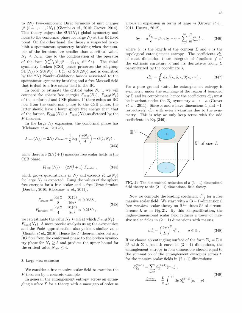
45

to 2Nf two-component Dirac fermions of unit chargesψi (i = 1, · · · , 2Nf ) (Giombi et al., 2016; Grover, 2014).This theory enjoys the SU(2Nf ) global symmetry andflows to the conformal phase for large Nf at the IR fixedpoint. On the other hand, the theory is suspected to ex-hibit a spontaneous symmetry breaking when the num-ber of the fermions are smaller than a critical value,Nf ≤ Ncrit, due to the condensation of the operator

of the form∑Nfi=1(ψi ψ

i − ψi+Nf ψi+Nf ). The chiral

symmetry broken (CSB) phase preserves the subgroupSU(Nf ) × SU(Nf ) × U(1) of SU(2Nf ) and is describedby the 2N2

f Nambu-Goldstone bosons associated to thespontaneous symmetry breaking and a free Maxwell fieldthat is dual to a free scalar field in the IR.

In order to estimate the critical value Ncrit, we willcompare the sphere free energies Fconf(Nf ), FCSB(Nf )of the conformal and CSB phases. If there exists an RGflow from the conformal phase to the CSB phase, thelatter should have a lower sphere free energy than thatof the former, FCSB(Nf ) < Fconf(Nf ) as dictated by theF -theorem.

In the large Nf expansion, the conformal phase has(Klebanov et al., 2012c),

Fconf(Nf ) = 2Nf Fferm +1

2log

(πNf

4

)+O(1/Nf ) ,

(343)

while there are (2N2f +1) massless free scalar fields in the

CSB phase,

FCSB(Nf ) =(2N2

f + 1)Fscalar , (344)

which grows quadratically in Nf and exceeds Fconf(Nf )for large Nf as expected. Using the values of the spherefree energies for a free scalar and a free Dirac fermion(Dowker, 2010; Klebanov et al., 2011),

Fscalar =log 2

8− 3ζ(3)

16π2≈ 0.0638 ,

Ffermion =log 2

4+

3ζ(3)

8π2≈ 0.2189 ,

(345)

we can estimate the value Nf ≈ 4.4 at which FCSB(Nf ) =Fconf(Nf ). A more precise analysis using the ε-expansionand the Pade approximation also yields a similar value(Giombi et al., 2016). Hence the F -theorem rules out anyRG flow from the conformal phase to the broken symme-try phase for Nf ≥ 5 and predicts the upper bound forthe critical value Ncrit ≤ 4.

3. Large mass expansion

We consider a free massive scalar field to examine theF -theorem by a concrete example.

In general, the entanglement entropy across an entan-gling surface Σ for a theory with a mass gap of order m

allows an expansion in terms of large m (Grover et al.,2011; Huerta, 2012),

SΣ = α`Σε

+ β m`Σ − γ +

∞∑n=0

cΣ−2n−1

m2n+1, (346)

where `Σ is the length of the contour Σ and γ is thetopological entanglement entropy. The coefficients cΣ−iof mass dimension i are integrals of functions f ofthe extrinsic curvature κ and its derivatives along Σparametrized by the coordinate s,

cΣ−i =

∮Σ

ds f(κ, ∂sκ, ∂2sκ, · · · ) . (347)

For a pure ground state, the entanglement entropy issymmetric under the exchange of the region A boundedby Σ and its complement, hence the coefficients cΣ−i mustbe invariant under the Z2 symmetry κ → −κ (Groveret al., 2011). Since κ and s have dimensions 1 and −1,respectively, cΣ−i with even i vanishes due to the sym-metry. This is why we only keep terms with the oddcoefficients in Eq. (346).

S1 of size L

A

A

R2,1

FIG. 21 The dimensional reduction of a (3 + 1)-dimensionalfield theory to the (2 + 1)-dimensional field theory.

Now we compute the leading coefficient cΣ−1 for a freemassive scalar field. We start with a (3 + 1)-dimensionalfree massless scalar theory on R2,1 times S1 of circum-ference L as in Fig. 21. By this compactification, thehigher-dimensional scalar field reduces a tower of mas-sive scalar fields in (2 + 1) dimensions with masses,

m2n =

(2π

L

)2

n2 , n ∈ Z . (348)

If we choose an entangling surface of the form Σ2 = Σ×S1 with Σ a smooth curve in (3 + 1) dimensions, theentanglement entropy in four dimensions should equal tothe summation of the entanglement entropies across Σfor the massive scalar fields in (2 + 1) dimensions:

S(3+1)Σ2

=∑n∈Z

S(2+1)Σ (mn) ,

L→∞−−−−→ L

π

∫ 1/ε

0

dpS(2+1)Σ (m = p) ,

(349)

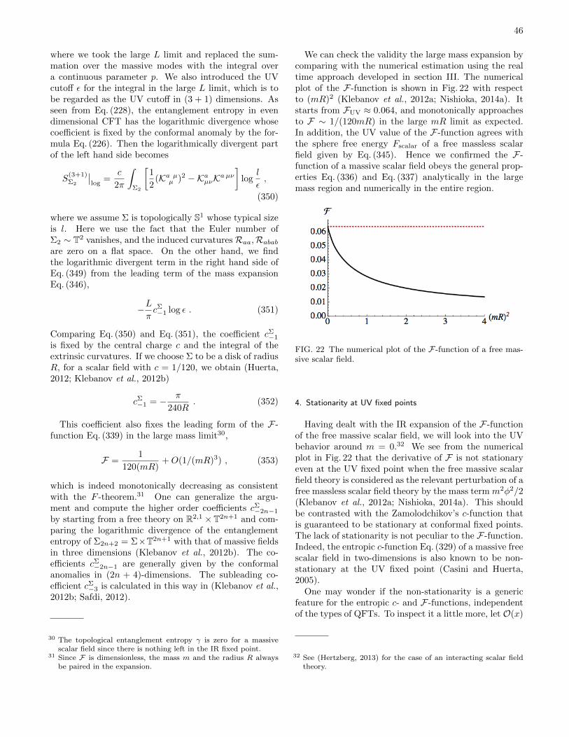
46

where we took the large L limit and replaced the sum-mation over the massive modes with the integral overa continuous parameter p. We also introduced the UVcutoff ε for the integral in the large L limit, which is tobe regarded as the UV cutoff in (3 + 1) dimensions. Asseen from Eq. (228), the entanglement entropy in evendimensional CFT has the logarithmic divergence whosecoefficient is fixed by the conformal anomaly by the for-mula Eq. (226). Then the logarithmically divergent partof the left hand side becomes

S(3+1)Σ2

∣∣log

=c

2π

∫Σ2

[1

2(Ka µµ )2 −KaµνKaµν

]log

l

ε,

(350)

where we assume Σ is topologically S1 whose typical sizeis l. Here we use the fact that the Euler number ofΣ2 ∼ T2 vanishes, and the induced curvaturesRaa,Rababare zero on a flat space. On the other hand, we findthe logarithmic divergent term in the right hand side ofEq. (349) from the leading term of the mass expansionEq. (346),

−LπcΣ−1 log ε . (351)

Comparing Eq. (350) and Eq. (351), the coefficient cΣ−1

is fixed by the central charge c and the integral of theextrinsic curvatures. If we choose Σ to be a disk of radiusR, for a scalar field with c = 1/120, we obtain (Huerta,2012; Klebanov et al., 2012b)

cΣ−1 = − π

240R. (352)

This coefficient also fixes the leading form of the F-function Eq. (339) in the large mass limit30,

F =1

120(mR)+O(1/(mR)3) , (353)

which is indeed monotonically decreasing as consistentwith the F -theorem.31 One can generalize the argu-ment and compute the higher order coefficients cΣ−2n−1

by starting from a free theory on R2,1 ×T2n+1 and com-paring the logarithmic divergence of the entanglemententropy of Σ2n+2 = Σ×T2n+1 with that of massive fieldsin three dimensions (Klebanov et al., 2012b). The co-efficients cΣ−2n−1 are generally given by the conformalanomalies in (2n + 4)-dimensions. The subleading co-efficient cΣ−3 is calculated in this way in (Klebanov et al.,2012b; Safdi, 2012).

30 The topological entanglement entropy γ is zero for a massivescalar field since there is nothing left in the IR fixed point.

31 Since F is dimensionless, the mass m and the radius R alwaysbe paired in the expansion.

We can check the validity the large mass expansion bycomparing with the numerical estimation using the realtime approach developed in section III. The numericalplot of the F-function is shown in Fig. 22 with respectto (mR)2 (Klebanov et al., 2012a; Nishioka, 2014a). Itstarts from FUV ≈ 0.064, and monotonically approachesto F ∼ 1/(120mR) in the large mR limit as expected.In addition, the UV value of the F-function agrees withthe sphere free energy Fscalar of a free massless scalarfield given by Eq. (345). Hence we confirmed the F-function of a massive scalar field obeys the general prop-erties Eq. (336) and Eq. (337) analytically in the largemass region and numerically in the entire region.

FIG. 22 The numerical plot of the F-function of a free mas-sive scalar field.

4. Stationarity at UV fixed points

Having dealt with the IR expansion of the F-functionof the free massive scalar field, we will look into the UVbehavior around m = 0.32 We see from the numericalplot in Fig. 22 that the derivative of F is not stationaryeven at the UV fixed point when the free massive scalarfield theory is considered as the relevant perturbation of afree massless scalar field theory by the mass term m2φ2/2(Klebanov et al., 2012a; Nishioka, 2014a). This shouldbe contrasted with the Zamolodchikov’s c-function thatis guaranteed to be stationary at conformal fixed points.The lack of stationarity is not peculiar to the F-function.Indeed, the entropic c-function Eq. (329) of a massive freescalar field in two-dimensions is also known to be non-stationary at the UV fixed point (Casini and Huerta,2005).

One may wonder if the non-stationarity is a genericfeature for the entropic c- and F-functions, independentof the types of QFTs. To inspect it a little more, let O(x)

32 See (Hertzberg, 2013) for the case of an interacting scalar fieldtheory.

47

be a relevant scalar operator of dimension ∆ (≤ d) in d-dimensional CFT, and consider the relevant perturbationby the operator

IE = IUV + gO

∫ddx√gO(x) , (354)

which induces an RG flow from the UV fixed point theorydescribed by the action IUV to an IR fixed point. Theperturbative expansion of entanglement entropy aroundthe UV fixed point (gO = 0) should take the form,

S(gO) = SUV + s1 gO + s2 g2O +O(g3

O) . (355)

The leading order term is the integrated two-point func-tion of the modular Hamiltonian HA and the relevantoperator (Rosenhaus and Smolkin, 2014, 2015),

s1 = −2π

∫ddx√g 〈HAO(x)〉 . (356)

The modular Hamiltonian is non-local in general, butcan be expressed as the integral of a local integrand pro-portional to the stress tensor for a planar or sphericalentangling surface in CFT as given in Eq. (166). In thiscase, the first order term is expected to vanish, s1 = 0,for 〈Tµν(x)O(y)〉 = 0 in CFT (see Eq. (218)) (Rosenhausand Smolkin, 2014). Thus this perturbative argumentshows quite generally that entanglement entropy is sta-tionary at the UV fixed point. We record for the reader’sreference that the second order term s2 is non-vanishing,whose form is determined for a spherical entangling sur-face of radius R on Rd to be (Faulkner, 2015)

s2 = −R2(d−∆)π(d+1)/2(d−∆)Γ (d/2 + 1−∆)

2Γ (d+ 3/2−∆), (357)

for operators with ∆ ≥ d/2.The contradiction between the above general argument

and the numerical result for a free massive scalar fieldbegs some explanation. The origin of this puzzle may betraced back to our tacit assumption for the stress tensorbeing conformal invariant, i.e., Tµµ = 0 in deriving theexpansion Eq. (355) with the conformal perturbation the-ory. For a free scalar field, however, we have a family of

the stress tensors T(ξ)µν parameterized by a coupling con-

stant ξ for the curvature couplingRφ2 that can be addedto the action when lifting the theory from flat space-

time to a curved spacetime. T(ξ)µν is conformally invariant

(traceless) only when ξ = ξc ≡ (d − 2)/ (4(d− 1)) evenon flat spacetime. There is no a priori reason to prefer

the conformal stress tensor T(ξc)µν to the others in calcu-

lating entanglement entropy. The possibility of adoptingthe non-conformal stress tensors was examined by (Casiniet al., 2015b; Herzog and Nishioka, 2016; Lee et al., 2015),resulting in the speculation that the correct value of theleading coefficient s1 is given by Eq. (356) with the stress

tensor T(ξ=0)µν for the minimal coupling ξ = 0.

Furthermore, the stationarity of entanglement entropyis conjectured to break down when there exists an oper-ator Od−2 of dimension ∆ = d− 2 that can couple to thescalar curvature ROd−2 (Herzog and Nishioka, 2016). Itremains to be clarified under what condition the entropicc- and F-functions become the stronger version of a C-function.

E. The entropic C-theorems in d ≥ 4 dimensions

We have seen that the entropic c- and F -theorems in(1 + 1) and (2 + 1) dimensions follow from the strongsubadditivity of entanglement entropy and the Lorentzinvariance of QFTs. One may then expect the a-theoremin (3+1) dimensions similarly follows from the same argu-ment. There however are obstacles in the generalizationto the higher dimensional cases which make the strongsubadditivity inequalities be trivial due to logarithmicdivergences coming from singular surfaces of intersectingboosted spheres (Casini and Huerta, 2012).

To overcome this difficulty, Casini et al. (2017a) andLashkari (2017) consider a difference of the entanglemententropies across a (d − 2)-sphere of radius R between atheory T along an RG flow and the UV CFT at its UVfixed point in d dimensions,

∆ST (R) ≡ ST (R)− SUV(R) . (358)

and define a new entanglement measure,

ST (R) ≡ [R∂R − (d− 2)] ∆ST (R) . (359)

The strong subadditivity Eq. (340) still holds for the dif-ference ∆ST (R) thanks to the Markov property of theCFT vacuum that saturates the strong subadditivity forentangling regions whose boundaries are located on alight cone (Casini et al., 2017b). Furthermore, the UVdivergences from the singular intersections are canceledout in the difference ∆ST (R), which results in the mono-tonicity of ST (R) in any dimension,

S ′T (R) ≤ 0 . (360)

This new measure reduces to the entropic c- and the F-functions when d = 2 and d = 3, respectively, and theinequality Eq. (360) guarantees their monotonicities.

Now we move onto the four-dimensional case and seewhat we are able to draw from the inequality Eq. (360).Recalling Eq. (225) and Eq. (226), the entanglement en-tropy across a two-sphere of radius R in CFT4 is givenby

S(R)|CFT = α4πR2

ε2− a log

R

ε. (361)

We are interested in the difference of the a-anomaliesbetween the UV and IR fixed points of an RG flow,

48

hence consider the IR CFT as a theory T for the mea-sure ST (R). Evaluating the inequality Eq. (360) with thefixed point value Eq. (361) we find

S ′IR(R) = 2(aIR − aUV)1

R≤ 0 , (362)

which proves the weak version of the a-theorem Eq. (325)(Casini et al., 2017a).33

In d ≥ 4 dimensions Giombi and Klebanov (2015) con-jecture the generalized F -theorem, stating the general-ized F coefficient defined by

F ≡ sin

(π d

2

)log Z[Sd] , (363)

decreases along an RG flow,

FUV ≥ FIR . (364)

We want to examine if the monotonicity Eq. (360) in d ≥4 dimensions also proves the conjecture as in the lower-dimensional cases.

Noting that the small R limit that corresponds to theUV region of an RG flow, we find ST (0) = 0 for anytheory T . Then the inequality Eq. (360) implies

ST (R) ≤ 0 . (365)

By choosing T be the IR theory, it leads to an inequalitythat contains the UV divergence of order O(1/εd−4) asseen from the UV structures Eq. (228) and (230) in CFT.Hence we are not able to derive a relation between finitevalues of the form, Eq. (364).

One may still hope to regularize the UV divergencein Eq. (365) by the dimensional regularization and de-rive the finite relation Eq. (364). Indeed the equalityEq. (255) leads to

F |CFT = sin

(π d

2

)SCFT(R) , (366)

and one may recast Eq. (365) into the inequality for thefixed point values FUV and FIR. While the resulting in-equality agrees with Eq. (364) for 2 < d < 4, it becomesrather the opposite, FIR ≥ FUV for 4 < d < 6, which is inapparent contradiction to the free field results (Giombiand Klebanov, 2015). This conflict stems from the factthat the inequality Eq. (365) holds only in the presence ofthe UV divergences. It is challenging, at the time of writ-ing this article, to derive an inequality for the dimension-ally regularized entanglement entropies, which hopefullyproves the generalized F -theorem in higher dimensions.

33 Solodukhin (2013) uses the dilation effective action to prove thea-theorem using the entanglement entropy of a spherical entan-gling surface.

F. Holographic RG flow

In this section, we switch gears to consider a simpleclass of holographic RG flows that are dual to Lorentzinvariant QFTs in d dimensions, and examine the entan-glement entropy across a sphere under the flows (Kle-banov et al., 2012b; Liu and Mezei, 2013a,b). A comple-mentary test of the F -theorem in three dimensions willbe performed in the holographic systems.

1. Domain wall and gapped RG flows

The most general metric holographically describing anRG flow on a flat space R1,d−1 is of Poincare type:

ds2 =L2

z2

[dz2

f(z)− dt2 + d~x2

d−1

], (367)

where d~x2d−1 is the metric of the (d− 1)-dimensional flat

space Rd−1. We require the function f(z) approaches toa constant (that we choose to one here),

f(z) −−−→z→0

1 . (368)

so that the metric asymptotes to an AdSd+1 space-timeof radius L near the boundary z = 0.

We are interested in a physical situation where themetric is a solution to the Einstein equation, hence notevery function f(z) satisfying Eq. (368) is of our inter-est. Moreover we should exclude unphysical solutions byintroducing a physically sensible condition.

Suppose the metric Eq. (367) describing an RG flowis a solution in the Einstein gravity coupled to matterfields,

I =1

16πGN

∫dd+1x

√−g [R+ Lmatter] , (369)

where Lmatter is the Lagrangian of the matter fields.The metric Eq. (367) with an arbitrary function f(z)can be a solution to the Einstein equation,34 Tmatter

µν =Rµν − Rgµν/2, by tuning the bulk matter stress ten-sor Tmatter

µν or equivalently the matter Lagrangian Lmatter

properly. This construction, however, often leads to un-reasonable solutions that we may want to rule out onthe physical ground. It is common practice to imposethe null energy condition for making a theory of gravityphysically sensible (see e.g. (Hawking and Ellis, 2011)):

Tmatterµν ξµξν ≥ 0 . (370)

This condition must be met for any future directed nullvector ξµ (ξ2 = 0).

34 Our definition of the stress tensor in Lorentzian signature isTµν = 2√

−gδIδgµν

.

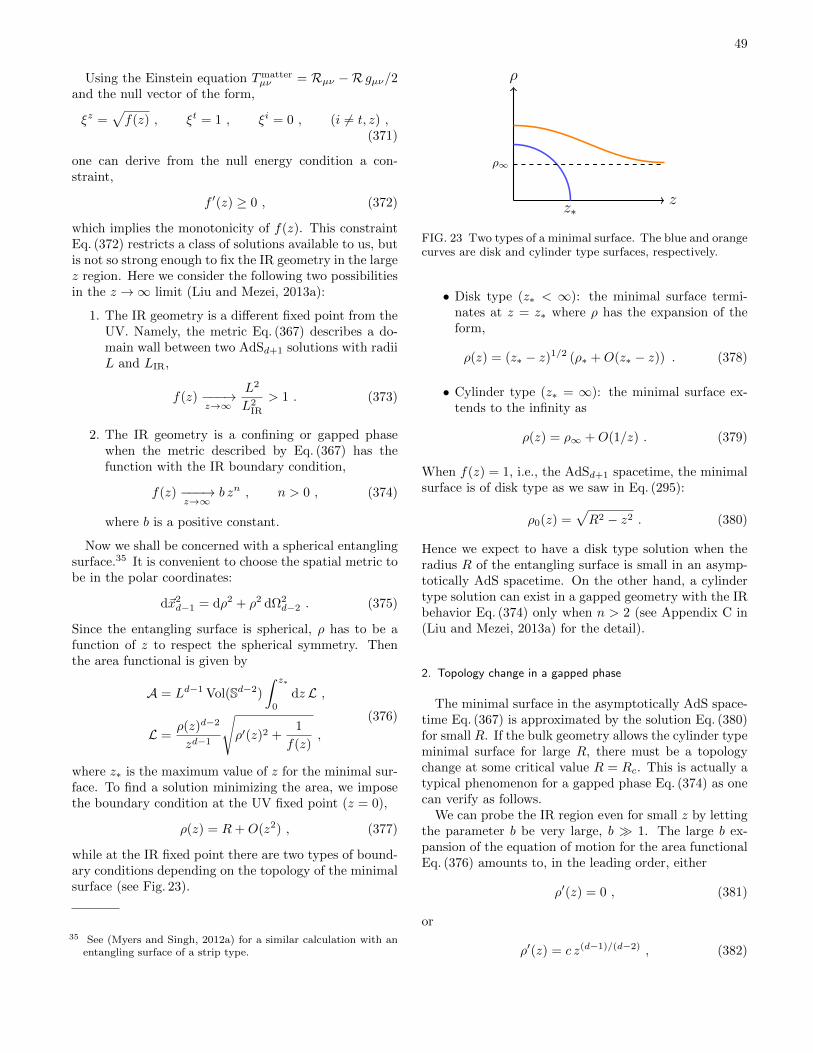
49

Using the Einstein equation Tmatterµν = Rµν −R gµν/2

and the null vector of the form,

ξz =√f(z) , ξt = 1 , ξi = 0 , (i 6= t, z) ,

(371)

one can derive from the null energy condition a con-straint,

f ′(z) ≥ 0 , (372)

which implies the monotonicity of f(z). This constraintEq. (372) restricts a class of solutions available to us, butis not so strong enough to fix the IR geometry in the largez region. Here we consider the following two possibilitiesin the z →∞ limit (Liu and Mezei, 2013a):

1. The IR geometry is a different fixed point from theUV. Namely, the metric Eq. (367) describes a do-main wall between two AdSd+1 solutions with radiiL and LIR,

f(z) −−−→z→∞

L2

L2IR

> 1 . (373)

2. The IR geometry is a confining or gapped phasewhen the metric described by Eq. (367) has thefunction with the IR boundary condition,

f(z) −−−→z→∞

b zn , n > 0 , (374)

where b is a positive constant.

Now we shall be concerned with a spherical entanglingsurface.35 It is convenient to choose the spatial metric tobe in the polar coordinates:

d~x2d−1 = dρ2 + ρ2 dΩ2

d−2 . (375)

Since the entangling surface is spherical, ρ has to be afunction of z to respect the spherical symmetry. Thenthe area functional is given by

A = Ld−1 Vol(Sd−2)

∫ z∗

0

dz L ,

L =ρ(z)d−2

zd−1

√ρ′(z)2 +

1

f(z),

(376)

where z∗ is the maximum value of z for the minimal sur-face. To find a solution minimizing the area, we imposethe boundary condition at the UV fixed point (z = 0),

ρ(z) = R+O(z2) , (377)

while at the IR fixed point there are two types of bound-ary conditions depending on the topology of the minimalsurface (see Fig. 23).

35 See (Myers and Singh, 2012a) for a similar calculation with anentangling surface of a strip type.

z

ρ

z∗

ρ∞

FIG. 23 Two types of a minimal surface. The blue and orangecurves are disk and cylinder type surfaces, respectively.

• Disk type (z∗ < ∞): the minimal surface termi-nates at z = z∗ where ρ has the expansion of theform,

ρ(z) = (z∗ − z)1/2 (ρ∗ +O(z∗ − z)) . (378)

• Cylinder type (z∗ = ∞): the minimal surface ex-tends to the infinity as

ρ(z) = ρ∞ +O(1/z) . (379)

When f(z) = 1, i.e., the AdSd+1 spacetime, the minimalsurface is of disk type as we saw in Eq. (295):

ρ0(z) =√R2 − z2 . (380)

Hence we expect to have a disk type solution when theradius R of the entangling surface is small in an asymp-totically AdS spacetime. On the other hand, a cylindertype solution can exist in a gapped geometry with the IRbehavior Eq. (374) only when n > 2 (see Appendix C in(Liu and Mezei, 2013a) for the detail).

2. Topology change in a gapped phase

The minimal surface in the asymptotically AdS space-time Eq. (367) is approximated by the solution Eq. (380)for small R. If the bulk geometry allows the cylinder typeminimal surface for large R, there must be a topologychange at some critical value R = Rc. This is actually atypical phenomenon for a gapped phase Eq. (374) as onecan verify as follows.

We can probe the IR region even for small z by lettingthe parameter b be very large, b 1. The large b ex-pansion of the equation of motion for the area functionalEq. (376) amounts to, in the leading order, either

ρ′(z) = 0 , (381)

or

ρ′(z) = c z(d−1)/(d−2) , (382)

50

for a constant c. The solution to the second equationdiverges for large z and is not acceptable as a minimalsurface while the solution to the first implies a cylindertype minimal surface. The topology change of the min-imal surface is observed numerically in many examples(Klebanov et al., 2012b; Liu and Mezei, 2013a,b).

The area of the cylinder type minimal surface may beevaluated in the system with a large gap (b 1) bydividing the calculation into the UV part z ≤ zb ≡ b−1/n

and the IR part z > zb. In the UV region, the solutionis close to the disk solution Eq. (380) in the AdS spacewhile it approaches to a constant in the IR region. Takinginto account the continuity at z = zb, it is reasonable toapproximate the solution by the piecewise function,

ρ(z) =

ρ0(z) (z ≤ zb) ,ρ0(zb) (z > zb) .

(383)

Now the area consists of two parts, A = Az≤zb +Az≥zb ,where the UV part is approximated in the large b limitby

Az≤zb =

∫ zb

ε

dzρ0(z)d−2(ρ′0(z)2 + 1)1/2

zd−1

·[1− b zn

2(ρ′0(z)2 + 1)

],

(384)

while the IR part becomes

Az≥zb =

∫ ∞zb

dzρ0(zb)

d−2

b1/2 zd−1+n/2. (385)

Using the dimensional regularization assuming n is largeenough, we have the expansion for zb 1,

A =1

(2d+ n− 4)

[2

(R

zb

)d−2

− (d− 2)

(R

zb

)d−4

+ · · ·

].

(386)

The entanglement entropy across a sphere of radius R isLd−1Vol(Sd−2)/(4GN ) times larger that this area. Com-pared with Eq. (176) for a free massive scalar field, theparameter zb allows for interpretation as a gap scale mas expected.

Similar topology change can be observed for a stripentangling region in a gapped system where the entan-gling surface is two parallel planes. There are two typesof extremal surfaces, one with a connected surface, theother with two disconnected surfaces terminate on the IRboundary of the gapped geometry. The topology changebetween these two types of surfaces is interpreted as aconfinement/deconfinement phase transition in a confin-ing gauge theory (Klebanov et al., 2008; Nishioka andTakayanagi, 2007; Pakman and Parnachev, 2008).

3. Testing the F -theorem in holography

As we saw in section VIII.D, the proof of the F -theorem was based on the Lorentz invariance and thestrong subadditivity of entanglement entropy that re-places the role of unitarity in QFT. The same argumentfor the proof remains to work in a holographic systemas well just by resorting to the strong subadditivity ofthe Ryu-Takayanagi formula (for the static case in sec-tion VII.C.2). Nevertheless, it is worthwhile examiningthe validity of the F -theorem from the holographic pointof view to draw implications for the interplay betweenunitarity in QFT and its counterpart in the dual gravity.

First let us consider a holographic gapped systemwith a large gap that we have dealt with in the previ-ous subsection. The renormalized entanglement entropy,Eq. (339), across a sphere of large radius is calculatedfrom Eq. (386) with d = 3 as,

F(R) =π L2

(n+ 2)GN

zbR

+O((zb/R)3

). (387)

This result should be compared with the typical behaviorof the F-function in the large gap limit given in Eq. (353)for a free massive scalar. Note that the value of F (thesphere free energy) at the UV fixed point of the holo-graphic RG flow is FUV = πL2/(2GN ) (see Eq. (300)),which is always greater than Eq. (387) in the large gapsystem with zb R. We thus find this type of holo-graphic RG flows is consistent with the F -theorem.

The next example to consider is a domain wall RG flowinterpolating two closely separated fixed points withouta gap (Liu and Mezei, 2013a). Such a solution can be re-alized by choosing the function f(z) in the general metricEq. (367) to be the form,

f(z) = 1 + η g(z) , η =L2

L2IR

− 1 1 , (388)

and imposing the boundary conditions at the UV and IRregions,

g(z) −−−→z→0

0 , g(z) −−−→z→∞

1 . (389)

The null energy condition Eq. (372) indicates g(z) be amonotonically increasing function,

g′(z) ≥ 0 . (390)

In this setup, we are allowed to expand the solution ofthe equation of motion of the area functional Eq. (376)around the UV solution Eq. (380),

ρ(z) = ρ0(z) + η ρ1(z) +O(η2) , (391)

and it follows the expansion of the area functional,

A = A0 + η A1 +O(η2) . (392)

51

We now focus on the d = 3 case to inspect the behav-ior of the F-function. Varying Eq. (376) around the UVsolution, we obtain the subleading term of the form36

A1 = 2πL2

∫ R

0

dz g(z)δLδf

∣∣∣∣f=1, ρ=ρ0

,

= −πL2

R

∫ R

0

dzR2 − z2

z2g(z) .

(393)

This integral is UV divergent due to the contribution nearthe UV boundary, z = 0, but we can regularized it withthe F-function and find the leading correction,

∆F(R) = −η πL2

2GN

∫ 1

0

dz g(zR) . (394)

which is always non-positive due to Eq. (390). We thusfind the F-function of the domain wall solution decreasesas R increases. Furthermore, the leading correctionmatches the difference between the UV and IR free en-ergies,

∆F(R→∞) = −η πL2

2GN,

= FIR − FUV +O(η2) .

(395)

Hence the domain wall RG flow realizes the strong ver-sion of the F -theorem.37

We note that the monotonicity of the F-function is adirect consequence of the null energy condition Eq. (372)in this holographic RG flow while it follows in the fieldtheoretic derivation in section VIII.D from the strongsubadditivity that is substituted by the minimality con-dition for the Ryu-Takayanagi surface. The derivationfor Eq. (394) indicates that the minimality condition isnot enough to prove the monotonicity of the F-functionin holography. To our best knowledge, no holographicproofs of the strong version of the F -theorem are known,hence it is desirable to elucidate it with the null energycondition along the line of (Freedman et al., 1999; Gi-rardello et al., 1998) beyond the perturbative level.

G. Supersymmetric Renyi entropies

We will conclude this section with a comment on someexact results for entanglement and Renyi entropies in in-teracting field theories with supersymmetries.

36 There are contributions from the boundaries at z = z∗ and z = 0,which turns out to be negligible for d ≤ 4 (Liu and Mezei, 2013a).

37 The entanglement entropy of a holographic RG flow describing arelevantly perturbed CFT is shown to have the expansion of theform Eq. (355) with s1 = 0 and supports the strongest versionof the F -theorem at least around the UV fixed point when thedimension of the relevant operator is close to three (Taylor andWoodhead, 2016a,b).

Calculating the exact value of entanglement entropyin QFTs is generally an intractable task unless theoriesare free and the entangling surface preserves a rotationalsymmetry around it. The difficulty is most manifestin the replica method where the conical singularity onthe entangling surface prevents us from carrying out theperturbative calculation in a conventional manner. Onthe other hand, there are powerful computational tech-nique, called supersymmetric localization, in supersym-metric field theories that allows the exact calculation ofthe partition function and a certain class of correlationfunctions by reducing the infinite-dimensional path inte-gral to a finite-dimensional one (see (Dumitrescu, 2017;Pufu, 2016; Willett, 2017) for reviews). To apply su-persymmetric localization, a supersymmetric field theorymust be placed on manifolds preserving enough numberof supersymmetries.

A simple example is a round sphere and the resultingsupersymmetric partition function Zsusy[Sd] turns out tobe the partition function Z[Sd] of the supersymmetricfield theory at the IR fixed point. Provided the rela-tion Eq. (255) between the entanglement entropy acrossa round sphere and the sphere partition function Z[Sd]for CFTs, it is possible to calculate the exact value ofentanglement entropy for a class of supersymmetric fieldtheories (Jafferis et al., 2011; Pufu, 2016).

Given the success of the entanglement entropy, onemay wonder if the same story applies to the Renyi en-tropy, Eq. (147), for supersymmetric field theories as well.Such an attempt would fail as supersymmetries are com-pletely broken on the n-fold cover of the d-sphere Sdn (de-fined by Eq. (250)), thus the supersymmetric localizationcan not be applied.

In order to leverage the supersymmetric localizationtechnique, we would rather tailor the definition of theRenyi entropy so as to be compatible with supersymme-tries. Namely, we define the supersymmetric Renyi en-tropy Ssusy

n for supersymmetric conformal field theoriesby (Nishioka and Yaakov, 2013),

Ssusyn ≡ 1

1− nlog

∣∣∣∣ Zsusy[Sdn]

(Zsusy[Sd])n

∣∣∣∣ , (396)

where Zsusy[Sd] is the supersymmetric partition functionon Sdn with background fields turned on to preserve a partof supersymmetries.38 This definition takes the sameform as the Renyi entropy, Eq. (147), across a sphericalentangling surface Sd−2 in CFT on Rd (see Eq. (253)),except for the partition function being replaced with thesupersymmetric one.39

38 The effect of the background fields vanishes for CFT on a roundsphere, hence Zsusy[Sd] = Z[Sd].

39 The absolute value inside the logarithm ensures that the super-symmetric Renyi entropy is universal at least in three dimensions(Closset et al., 2012).

52

The explicit formula for Zsusy[Sd] is given by an inte-gration over finite-dimensional matrix variables that de-pends on the spacetime dimensions, the rank of the gaugegroup, and the matter contents of supersymmetric fieldtheories, but we are not concerned with the explicit formhere. Instead of giving examples, we recap the universalaspects of the supersymmetric Renyi entropy for N = 2supersymmetric field theories with the global U(1)R sym-metry in three dimensions (Nishioka and Yaakov, 2013):

• The expansion around n = 1 takes the form,

Ssusyn = S1 +

π2

16τRR (n− 1) +O

((n− 1)2

), (397)

where τRR appears as the coefficients CJ =τRR/(4π

2) and CT = 3τRR/(2π2) in the correlators

of the U(1)R-symmetry current j(R)µ and the stress

tensor given by Eq. (215) and Eq. (216). Comparedwith the expansion Eq. (259) of the Renyi entropywith the first derivative Eq. (260) in d = 3 dimen-sions,

Sn = S1 +π2

8τRR (n− 1) +O

((n− 1)2

), (398)

we find a factor two discrepancy at the leading or-der coefficient. This is due to the effect of the back-ground gauge field for the U(1)R symmetry thatis turned on to maintain supersymmetries on Sdn.Hence the supersymmetric Renyi entropy is differ-ent from the Renyi entropy when n 6= 1 in general.

• For theories with gauge groups of rank N , the ndependence simplifies in the large-N limit,

Ssusyn =

3n+ 1

4nS1 , (399)

A curious fact is that the ratio Hn ≡ Ssusyn /S1 sat-

isfies the inequalities Eq. (56)-(59) of the Renyi en-tropies.

• For a certain class of superconformal field theo-ries allowing for the holographic dual description,the gravity dual of the supersymmetric Renyi en-tropy is described by the charged topological AdS4

black hole that is a half-BPS solution in the N = 2U(1) gauged four-dimensional supergravity (Huanget al., 2014; Nishioka, 2014b).

• The description by codimension-two defects livingon the entangling surface is manifest (Nishioka andYaakov, 2017).

The supersymmetric Renyi entropies and their grav-ity duals have been explored with some applications inthe other dimensions (Alday et al., 2015; Giveon andKutasov, 2016; Hama et al., 2014; Huang and Zhou,2015; Mori, 2016; Nian and Zhou, 2016; Yankielowicz and

Zhou, 2017; Zhou, 2015, 2016). We believe they shednew light on understanding the nature of quantum en-tanglement in QFT and the fundamental connection ofquantum states to the holographic spacetime.

ACKNOWLEDGMENTS

I am grateful to Shamik Banerjee, Chris Herzog,Igor Klebanov, Yuki Nakaguchi, Silviu Pufu, Ben Safdi,Tadashi Takayanagi, Kazuya Yonekura and Amos Yaromfor stimulating collaborations on the various works partlyreviewed in this article, and to Horacio Casini, MarinaHuerta, Noriaki Ogawa for valuable comments and dis-cussions. I would also like to thank the organizers of the18th APCTP Winter School on Fundamental Physics, the9th Asian Winter School on String, Particles and Cosmol-ogy and the 6th Advanced String School at Puri for givingme the opportunities to deliver lectures and also the par-ticipants for many comments and questions. This workwas supported in part by JSPS Grant-in-Aid for YoungScientists (B) No.15K17628 and JSPS Grant-in-Aid forScientific Research (A) No.16H02182.

Appendix A: Real time formalism for fermions

In this appendix, we extend the real time formalism,developed for free bosonic systems in section III, to freefermionic systems.

1. Fermionic system on lattice

We consider a quadratic Hamiltonian of fermions onlattice labeled by an integer i = 1, · · · , N ,

H =

N∑i,j=1

ψ†i Mij ψj , (A1)

with fermionic operators satisfying the anti-commutationrelation ψi, ψ†j = δij . The Hermitian matrix M can be

diagonalized to M = U†∆U by a unitary matrix U , thenthe Hamiltonian becomes

H =

N∑l=1

λl ψ†l ψl , ψ = U ψ , (A2)

where λl are real diagonal entries of ∆ and the new opera-tors ψl satisfy the anti-commutation relation ψl, ψ†m =δlm. We let S(+) and S(−) be the sets of indices for posi-tive and negative eigenvalues, respectively. We define theground state as the Dirac sea

|0〉 ≡∏

l∈S(−)

ψl|0〉 , (A3)

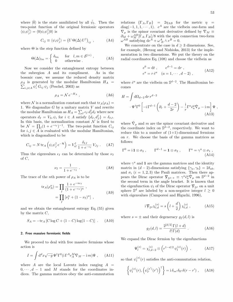
53

where |0〉 is the state annihilated by all ψl. Then thetwo-point function of the original fermionic operators〈ψiψ†j 〉 = 〈0|ψiψ†j |0〉 is

Cij ≡ 〈ψiψ†j 〉 =(U Θ(∆)U†

)ij, (A4)

where Θ is the step function defined by

Θ(∆)lm =

δlm for l,m ∈ S(+) ,0 otherwise .

(A5)

Now we consider the entanglement entropy betweenthe subregion A and its compliment. As in thebosonic case, we assume the reduced density matrixρA is generated by the modular Hamiltonian HA =∑i,j∈A ψ

†i Gij ψj (Peschel, 2003) as

ρA = N e−HA , (A6)

where N is a normalization constant such that trA(ρA) =1. We diagonalize G by a unitary matrix V and rewritethe modular Hamiltonian as HA =

∑I εI d

†IdI where new

operators dI = VIi ψi for i ∈ A satisfy dI , d†J = δIJ .In this basis, the normalization constant N is fixed tobe N =

∏I(1 + e−εI )−1. The two-point function Cij

for i, j ∈ A is evaluated with the modular Hamiltonian,which is diagonalized to be

Cij = N trA

(ψiψ

†j e−H)

= V †iIδIJ

1 + e−εIVJj . (A7)

Thus the eigenvalues εI can be determined by those νIof C,

νI =1

1 + e−εI. (A8)

The trace of the nth power of ρA is to be

trA(ρnA) =∏I

1 + e−nεI

(1 + e−εI )n,

=∏I

[νnI + (1− νI)n] ,(A9)

and we obtain the entanglement entropy Eq. (55) givenby the matrix C,

SA = −trA [C logC + (1− C) log(1− C)] . (A10)

2. Free massive fermionic fields

We proceed to deal with free massive fermions whoseaction is

I =

∫ddx√−gΨ†Γ0(i ΓAeMA ∇M − im)Ψ , (A11)

where A are the local Lorentz index ranging A =0, · · · , d − 1 and M stands for the coordinates in-dices. The gamma matrices obey the anti-commutation

relations ΓA,ΓB = 2ηAB for the metric η =diag(−1, 1, 1, · · · , 1). eA are the vielbein one-form and∇µ is the spinor covariant derivative defined by ∇M ≡∂M + ωABM [ΓA,ΓB ]/8 with the spin connection two-formωAB satisfying deA + ωAB ∧ eB = 0.

We concentrate on the case in d ≥ 3 dimensions. See,for example, (Herzog and Nishioka, 2013) for the imple-mentation in two dimensions. We put the theory on theradial coordinates Eq. (108) and choose the vielbein as

e0 = dt , ed−1 = dr ,

ea = r ea (a = 1, · · · , d− 2) ,(A12)

where ea are the vielbein on Sd−2. The Hamiltonian be-comes

H =

∫dΩd−2 dr rd−2

·Ψ†Γ0

[−i Γd−1

(∂r +

d− 2

2r

)− i

rΓaeµa∇µ − im

]Ψ ,

(A13)

where ∇µ and m are the spinor covariant derivative andthe coordinate index on Sd−2, respectively. We want toreduce this to a number of (1+1)-dimensional fermionson r. We choose the basis of the gamma matrices asfollows:

Γ0 = i1⊗ σ3 , Γd−1 = 1⊗ σ2 , Γa = γa ⊗ σ1 ,(A14)

where γa and 1 are the gamma matrices and the identitymatrix in (d − 2)-dimensions satisfying γa, γb = 2δab,and σi (i = 1, 2, 3) the Pauli matrices. Then there ap-pears the Dirac operator ∇/ Sd−2 ≡ γaeµa∇µ on Sd−2 inthe second term in the angle bracket. It is known thatthe eigenfunction ψl of the Dirac operator ∇/ Sd on a unitsphere Sd are labeled by a non-negative integer l ≥ 0with eigenvalues (Camporesi and Higuchi, 1996),

i∇/ Sdχ(s)l,d = s

(l +

d

2

)χ

(s)l,d , (A15)

where s = ± and their degeneracy gf (d, l) is

gf (d, l) =2[d/2] Γ(l + d)

l! Γ(d). (A16)

We expand the Dirac fermion by the eigenfunctions

Ψ(s)l = χ

(s)l,d−2 ⊗

(r1−d/2 ψ

(s)l (r)

), (A17)

so that ψ(s)l (r) satisfies the anti-commutation relation,

ψ(s)l (r),

(ψ

(s′)l′ (r′)

)†= i δss′δll′δ(r − r′) , (A18)

54

and rewrite the Hamiltonian as the sum over the angularmodes,

H =

∞∑l=0

∑s=±

gf (d− 2, l)H(s)l , (A19)

with

H(s)l =

∫dr

[− i

2

(ψ

(s)l (r)

)†σ1 ∂rψ

(s)l (r)

+i

2∂r

(ψ

(s)l (r)

)†σ1 ψ

(s)l (r)

+s

r

(l +

d− 2

2

)(ψ

(s)l (r)

)†σ2 ψ

(s)l (r)

+m(ψ

(s)l (r)

)†σ3 ψ

(s)l (r)

].

(A20)

To discretize the radial coordinate r to lattice labeled byj = 1, 2, · · · , N with lattice spacing a, we replace

r → ja , δ(r − r′)→ δjka

,

ψ(s)l (r)→

ψ(s)l,j√a, ∂r ψ

(s)l (r)→

ψ(s)l,j+1 − ψ

(s)l,j

a,

(A21)

then the discretized Hamiltonian reads

H(s)l =

1

a

N∑j,k=1

(ψ

(s)l,j

)† (M

(s)l

)j,kψ

(s)l,k . (A22)

with the Hermitian matrix M(s)l given by(

M(s)l

)k,k=s

k

(l +

d− 2

2

)σ2 + (ma)σ3 ,(

M(s)l

)k,k+1

= −(M

(s)l

)k+1,k

= − i

2σ1 .

(A23)

Finally the entanglement entropy of the free massiveDirac fermion is given by the sum over the angular modesl,

SA =

∞∑l=0

∑s=±

gf (d− 2, l)S(s)l , (A24)

where S(s)l is the entropy of the lth mode given by the

formula Eq. (A10) with the two-point function C(s)l of the

form Eq. (A4) for the Hermitian matrix M(s)l Eq. (A23).

REFERENCES

Adesso, Gerardo, Davide Girolami, and Alessio Serafini(2012), “Measuring Gaussian quantum information andcorrelations using the Renyi entropy of order 2,” Physicalreview letters 109 (19), 190502.

Aharony, Ofer, Steven S. Gubser, Juan Martin Maldacena,Hirosi Ooguri, and Yaron Oz (2000), “Large N Field The-ories, String Theory and Gravity,” Phys.Rept. 323, 183–386, arXiv:hep-th/9905111 [hep-th].

Alday, Luis F, Paul Richmond, and James Sparks (2015),“The holographic supersymmetric Renyi entropy in five di-mensions,” JHEP 02, 102, arXiv:1410.0899 [hep-th].

Anselmi, D, D. Z. Freedman, Marcus T. Grisaru, and A. A.Johansen (1998), “Nonperturbative formulas for centralfunctions of supersymmetric gauge theories,” Nucl. Phys.B526, 543–571, arXiv:hep-th/9708042 [hep-th].

Aoki, Sinya, Takumi Iritani, Masahiro Nozaki, Tokiro Nu-masawa, Noburo Shiba, and Hal Tasaki (2015), “On theDefinition of Entanglement Entropy in Lattice Gauge The-ories,” JHEP 06, 187, arXiv:1502.04267 [hep-th].

Appelquist, Thomas, Andrew G. Cohen, and MartinSchmaltz (1999), “A New constraint on strongly cou-pled gauge theories,” Phys. Rev. D60, 045003, arXiv:hep-th/9901109 [hep-th].

Araki, H, and E. H. Lieb (1970), “Entropy inequalities,”Commun. Math. Phys. 18, 160–170.

Azeyanagi, Tatsuo, R. Loganayagam, and Gim SengNg (2017), “Holographic Entanglement for Chern-SimonsTerms,” JHEP 02, 001, arXiv:1507.02298 [hep-th].

Balakrishnan, Srivatsan, Thomas Faulkner, Zuhair U. Khand-ker, and Huajia Wang (2017), “A General Proof of theQuantum Null Energy Condition,” arXiv:1706.09432 [hep-th].

Barnes, Edwin, Kenneth A. Intriligator, Brian Wecht, andJason Wright (2004), “Evidence for the strongest versionof the 4d a-theorem, via a-maximization along RG flows,”Nucl. Phys. B702, 131–162, arXiv:hep-th/0408156 [hep-th].

Beigi, Salman (2013), “Sandwiched Renyi divergence satis-fies data processing inequality,” Journal of MathematicalPhysics 54 (12), 122202.

Benini, Francesco, Po-Shen Hsin, and Nathan Seiberg (2017),“Comments on global symmetries, anomalies, and dual-ity in (2 + 1)d,” JHEP 04, 135, arXiv:1702.07035 [cond-mat.str-el].

Bhattacharya, Jyotirmoy, Veronika E. Hubeny, MukundRangamani, and Tadashi Takayanagi (2015), “Entangle-ment density and gravitational thermodynamics,” Phys.Rev. D91 (10), 106009, arXiv:1412.5472 [hep-th].

Birrell, N D, and P. C. W. Davies (1982), Quantum Fieldsin Curved Space (Cambridge university press).

Bisognano, J J, and E. H. Wichmann (1975), “On the DualityCondition for a Hermitian Scalar Field,” J. Math. Phys. 16,985–1007.

Bisognano, J J, and E. H. Wichmann (1976), “On the DualityCondition for Quantum Fields,” J. Math. Phys. 17, 303–321.

de Boer, Jan, Manuela Kulaxizi, and Andrei Parnachev(2011), “Holographic Entanglement Entropy in LovelockGravities,” JHEP 1107, 109, arXiv:1101.5781 [hep-th].

Bombelli, Luca, Rabinder K. Koul, Joohan Lee, andRafael D. Sorkin (1986), “A Quantum Source of Entropyfor Black Holes,” Phys. Rev. D34, 373–383.

Bousso, Raphael, Horacio Casini, Zachary Fisher, and JuanMaldacena (2014), “Proof of a Quantum Bousso Bound,”Phys. Rev. D90 (4), 044002, arXiv:1404.5635 [hep-th].

Bousso, Raphael, Horacio Casini, Zachary Fisher, and JuanMaldacena (2015), “Entropy on a null surface for interact-ing quantum field theories and the Bousso bound,” Phys.

55

Rev. D91 (8), 084030, arXiv:1406.4545 [hep-th].Bousso, Raphael, Zachary Fisher, Jason Koeller, Stefan Le-

ichenauer, and Aron C. Wall (2016), “Proof of the Quan-tum Null Energy Condition,” Phys. Rev. D93 (2), 024017,arXiv:1509.02542 [hep-th].

Brown, Lowell S (1977), “Stress Tensor Trace Anomaly ina Gravitational Metric: Scalar Fields,” Phys. Rev. D15,1469.

Bueno, Pablo, and Robert C. Myers (2015), “Corner contri-butions to holographic entanglement entropy,” JHEP 08,068, arXiv:1505.07842 [hep-th].

Bueno, Pablo, Robert C. Myers, and William Witczak-Krempa (2015), “Universality of corner entanglement inconformal field theories,” Phys. Rev. Lett. 115, 021602,arXiv:1505.04804 [hep-th].

Calabrese, Pasquale, and John Cardy (2007), “QuantumQuenches in Extended Systems,” J. Stat. Mech. 0706,P06008, arXiv:0704.1880 [cond-mat.stat-mech].

Calabrese, Pasquale, and John Cardy (2009), “Entangle-ment Entropy and Conformal Field Theory,” J. Phys. A42,504005, arXiv:0905.4013 [cond-mat.stat-mech].

Calabrese, Pasquale, and John Cardy (2016), “Quantumquenches in 1+1 dimensional conformal field theories,”J. Stat. Mech. 1606 (6), 064003, arXiv:1603.02889 [cond-mat.stat-mech].

Calabrese, Pasquale, and John L. Cardy (2004), “Entangle-ment Entropy and Quantum Field Theory,” J. Stat. Mech.0406, P06002, arXiv:hep-th/0405152.

Calabrese, Pasquale, and John L. Cardy (2005), “Evolutionof entanglement entropy in one-dimensional systems,” J.Stat. Mech. 0504, P04010, arXiv:cond-mat/0503393 [cond-mat].

Camporesi, Roberto, and Atsushi Higuchi (1996), “On theEigen Functions of the Dirac Operator on Spheres andReal Hyperbolic Spaces,” J.Geom.Phys. 20, 1–18, arXiv:gr-qc/9505009 [gr-qc].

Camps, Joan (2014), “Generalized Entropy and HigherDerivative Gravity,” JHEP 1403, 070, arXiv:1310.6659[hep-th].

Cappelli, Andrea, Daniel Friedan, and Jose I. Latorre (1991),“C theorem and spectral representation,” Nucl. Phys.B352, 616–670.

Cardy, John, and Christopher P. Herzog (2014), “Univer-sal Thermal Corrections to Single Interval EntanglementEntropy for Two Dimensional Conformal Field Theories,”Phys. Rev. Lett. 112 (17), 171603, arXiv:1403.0578 [hep-th].

Cardy, John L (1988), “Is There a c-Theorem in Four-Dimensions?” Phys. Lett. B215, 749–752.

Casini, H, and M. Huerta (2004), “A Finite EntanglementEntropy and the C-Theorem,” Phys.Lett. B600, 142–150,arXiv:hep-th/0405111 [hep-th].

Casini, H, and M. Huerta (2005), “Entanglement and AlphaEntropies for a Massive Scalar Field in Two Dimensions,”J. Stat. Mech. 0512, P12012, arXiv:cond-mat/0511014.

Casini, H, and M. Huerta (2007), “Universal terms for the en-tanglement entropy in 2+1 dimensions,” Nucl. Phys. B764,183–201, arXiv:hep-th/0606256 [hep-th].

Casini, H, and M. Huerta (2009), “Entanglement Entropyin Free Quantum Field Theory,” J. Phys. A42, 504007,arXiv:0905.2562 [hep-th].

Casini, H, M. Huerta, and L. Leitao (2009), “Entan-glement entropy for a Dirac fermion in three dimen-sions: Vertex contribution,” Nucl. Phys. B814, 594–609,

arXiv:0811.1968 [hep-th].Casini, H, and Marina Huerta (2012), “On the RG Running

of the Entanglement Entropy of a Circle,” Phys.Rev. D85,125016, arXiv:1202.5650 [hep-th].

Casini, Horacio, Marina Huerta, and Robert C. Myers (2011),“Towards a Derivation of Holographic Entanglement En-tropy,” JHEP 05, 036, arXiv:1102.0440 [hep-th].

Casini, Horacio, Marina Huerta, Robert C. Myers, andAlexandre Yale (2015a), “Mutual information and the F -theorem,” JHEP 10, 003, arXiv:1506.06195 [hep-th].

Casini, Horacio, Marina Huerta, and Jose Alejandro Rosa-bal (2014), “Remarks on Entanglement Entropy for GaugeFields,” Phys. Rev. D89 (8), 085012, arXiv:1312.1183 [hep-th].

Casini, Horacio, F. D. Mazzitelli, and Eduardo Teste(2015b), “Area terms in entanglement entropy,” Phys. Rev.D91 (10), 104035, arXiv:1412.6522 [hep-th].

Casini, Horacio, Eduardo Teste, and Gonzalo Torroba(2017a), “Markov Property of the Conformal Field TheoryVacuum and the a-Theorem,” Phys. Rev. Lett. 118 (26),261602, arXiv:1704.01870 [hep-th].

Casini, Horacio, Eduardo Teste, and Gonzalo Torroba(2017b), “Modular Hamiltonians on the null plane and theMarkov property of the vacuum state,” J. Phys. A50 (36),364001, arXiv:1703.10656 [hep-th].

Castro, Alejandra, Stephane Detournay, Nabil Iqbal, andEric Perlmutter (2014), “Holographic Entanglement En-tropy and Gravitational Anomalies,” JHEP 1407, 114,arXiv:1405.2792 [hep-th].

Chen, Jiunn-Wei, Shou-Huang Dai, and Jin-Yi Pang (2015),“Strong Coupling Expansion of the Entanglement Entropyof Yang-Mills Gauge Theories,” arXiv:1503.01766 [hep-th].

Chung, Ming-Chiang, and Ingo Peschel (2000), “Density-matrix spectra for two-dimensional quantum systems,”Physical Review B 62 (7), 4191, cond-mat/0004222.

Closset, Cyril, Thomas T. Dumitrescu, Guido Festuccia, Zo-har Komargodski, and Nathan Seiberg (2012), “Con-tact Terms, Unitarity, and F -Maximization in Three-Dimensional Superconformal Theories,” JHEP 1210, 053,arXiv:1205.4142 [hep-th].

Cordova, Clay, Thomas T. Dumitrescu, and Kenneth Intrili-gator (2016), “Anomalies, renormalization group flows, andthe a-theorem in six-dimensional (1, 0) theories,” JHEP 10,080, arXiv:1506.03807 [hep-th].

Cordova, Clay, Thomas T. Dumitrescu, and Xi Yin(2015), “Higher Derivative Terms, Toroidal Compactifica-tion, and Weyl Anomalies in Six-Dimensional (2, 0) Theo-ries,” arXiv:1505.03850 [hep-th].

Deser, Stanley, and A. Schwimmer (1993), “Geometric Classi-fication of Conformal Anomalies in Arbitrary Dimensions,”Phys.Lett. B309, 279–284, arXiv:hep-th/9302047 [hep-th].

Di Francesco, P, P. Mathieu, and D. Senechal (1997), Con-formal Field Theory , Graduate Texts in ContemporaryPhysics (Springer-Verlag, New York).

Di Pietro, Lorenzo, Zohar Komargodski, Itamar Shamir, andEmmanuel Stamou (2016), “Quantum Electrodynamics ind = 3 from the ε Expansion,” Phys. Rev. Lett. 116 (13),131601, arXiv:1508.06278 [hep-th].

Di Pietro, Lorenzo, and Emmanuel Stamou (2017), “Scalingdimensions in QED3 from the ε-expansion,” JHEP 12, 054,arXiv:1708.03740 [hep-th].

Dong, Xi (2014), “Holographic Entanglement Entropy forGeneral Higher Derivative Gravity,” JHEP 1401, 044,arXiv:1310.5713 [hep-th].

56

Dong, Xi (2016), “The Gravity Dual of Renyi Entropy,” Na-ture Commun. 7, 12472, arXiv:1601.06788 [hep-th].

Dong, Xi, Aitor Lewkowycz, and Mukund Rangamani (2016),“Deriving covariant holographic entanglement,” JHEP 11,028, arXiv:1607.07506 [hep-th].

Donnelly, William (2014), “Entanglement Entropy and Non-abelian Gauge Symmetry,” Class. Quant. Grav. 31 (21),214003, arXiv:1406.7304 [hep-th].

Donnelly, William, and Aron C. Wall (2015), “EntanglementEntropy of Electromagnetic Edge Modes,” Phys. Rev. Lett.114 (11), 111603, arXiv:1412.1895 [hep-th].

Donnelly, William, and Aron C. Wall (2016), “Geometricentropy and edge modes of the electromagnetic field,” Phys.Rev. D94 (10), 104053, arXiv:1506.05792 [hep-th].

Dowker, J S (2010), “Entanglement Entropy for OddSpheres,” arXiv:1012.1548 [hep-th].

Duff, MJ (1994), “Twenty Years of the Weyl Anomaly,”Class.Quant.Grav. 11, 1387–1404, arXiv:hep-th/9308075[hep-th].

Dumitrescu, Thomas T (2017), “An introduction to su-persymmetric field theories in curved space,” J. Phys.A50 (44), 443005, arXiv:1608.02957 [hep-th].

Dur, W, G. Vidal, and J.I. Cirac (2000), “Three Qubits CanBe Entangled in Two Inequivalent Ways,” Phys.Rev. A62,062314.

Eisert, J (2006), “Entanglement in quantum information the-ory,” arXiv quant-ph/0610253v1.

Eisert, Jens, Marcus Cramer, and Martin B Plenio (2010),“Colloquium: Area laws for the entanglement entropy,” Re-views of Modern Physics 82 (1), 277.

Eisler, Viktor, and Ingo Peschel (2007), “Evolution of entan-glement after a local quench,” Journal of Statistical Me-chanics: Theory and Experiment 2007 (06), P06005.

Elvang, Henriette, and Marios Hadjiantonis (2015), “Exactresults for corner contributions to the entanglement entropyand Renyi entropies of free bosons and fermions in 3d,”Phys. Lett. B749, 383–388, arXiv:1506.06729 [hep-th].

Erdmenger, J, and H. Osborn (1997), “Conserved Currentsand the Energy Momentum Tensor in Conformally Invari-ant Theories for General Dimensions,” Nucl.Phys. B483,431–474, arXiv:hep-th/9605009 [hep-th].

Faulkner, Thomas (2015), “Bulk Emergence and the RG Flowof Entanglement Entropy,” JHEP 05, 033, arXiv:1412.5648[hep-th].

Faulkner, Thomas, Robert G. Leigh, Onkar Parrikar, andHuajia Wang (2016), “Modular Hamiltonians for DeformedHalf-Spaces and the Averaged Null Energy Condition,”JHEP 09, 038, arXiv:1605.08072 [hep-th].

Fei, Lin, Simone Giombi, and Igor R. Klebanov (2014), “Crit-ical O(N) models in 6−ε dimensions,” Phys. Rev. D90 (2),025018, arXiv:1404.1094 [hep-th].

Fradkin, Eduardo, and Joel E. Moore (2006), “Entanglemententropy of 2D conformal quantum critical points: hear-ing the shape of a quantum drum,” Phys. Rev. Lett. 97,050404, arXiv:cond-mat/0605683 [cond-mat.str-el].

Frank, Rupert L, and Elliott H Lieb (2013), “Monotonicity ofa relative Renyi entropy,” Journal of Mathematical Physics54 (12), 122201.

Freedman, D Z, S. S. Gubser, K. Pilch, and N. P. Warner(1999), “Renormalization Group Flows from HolographySupersymmetry and a C-Theorem,” Adv. Theor. Math.Phys. 3, 363–417, arXiv:hep-th/9904017.

Friedan, Daniel, and Anatoly Konechny (2010), “Gradientformula for the beta-function of 2d quantum field theory,”

J. Phys. A43, 215401, arXiv:0910.3109 [hep-th].Fursaev, Dmitri V (1994), “Spectral Geometry and One

Loop Divergences on Manifolds with Conical Singularities,”Phys. Lett. B334, 53–60, arXiv:hep-th/9405143.

Fursaev, Dmitri V (2006), “Proof of the Holographic Formulafor Entanglement Entropy,” JHEP 0609, 018, arXiv:hep-th/0606184 [hep-th].

Fursaev, Dmitri V, Alexander Patrushev, and Sergey N.Solodukhin (2013), “Distributional Geometry of SquashedCones,” Phys. Rev. D88 (4), 044054, arXiv:1306.4000 [hep-th].

Fursaev, Dmitri V, and Sergey N. Solodukhin (1995), “On theDescription of the Riemannian Geometry in the Presence ofConical Defects,” Phys. Rev. D52, 2133–2143, arXiv:hep-th/9501127.

Ghosh, Sudip, Ronak M Soni, and Sandip P. Trivedi (2015),“On the Entanglement Entropy for Gauge Theories,” JHEP09, 069, arXiv:1501.02593 [hep-th].

Gioev, Dimitri, and Israel Klich (2006), “Entanglement En-tropy of Fermions in Any Dimension and the Widom Con-jecture,” Phys.Rev.Lett. 96, 100503.

Giombi, Simone, and Igor R. Klebanov (2015), “Interpolatingbetween a and F ,” JHEP 03, 117, arXiv:1409.1937 [hep-th].

Giombi, Simone, Igor R. Klebanov, and Grigory Tarnopolsky(2016), “Conformal QEDd, F -Theorem and the ε Expan-sion,” J. Phys. A49 (13), 135403, arXiv:1508.06354 [hep-th].

Girardello, L, M. Petrini, M. Porrati, and A. Zaffaroni (1998),“Novel Local CFT and Exact Results on Perturbations ofN = 4 Super Yang-Mills from AdS Dynamics,” JHEP 12,022, arXiv:hep-th/9810126.

Giveon, Amit, and David Kutasov (2016), “Supersymmet-ric Renyi entropy in CFT2 and AdS3,” JHEP 01, 042,arXiv:1510.08872 [hep-th].

Graham, C Robin, and Edward Witten (1999), “Confor-mal anomaly of submanifold observables in AdS / CFTcorrespondence,” Nucl. Phys. B546, 52–64, arXiv:hep-th/9901021 [hep-th].

Greenberger, Daniel M, Michael A Horne, Abner Shimony,and Anton Zeilinger (1990), “Bells theorem without in-equalities,” Am. J. Phys 58 (12), 1131–1143.

Greenberger, Daniel M, Michael A Horne, and AntonZeilinger (1989), “Going beyond Bells theorem,” in Bellstheorem, quantum theory and conceptions of the universe(Springer) pp. 69–72.

Grover, Tarun (2014), “Entanglement Monotonicity and theStability of Gauge Theories in Three Spacetime Dimen-sions,” Phys. Rev. Lett. 112 (15), 151601, arXiv:1211.1392[hep-th].

Grover, Tarun, Ari M. Turner, and Ashvin Vishwanath(2011), “Entanglement Entropy of Gapped Phases andTopological Order in Three Dimensions,” Phys.Rev. B84,195120, arXiv:1108.4038 [cond-mat.str-el].

Gubser, S S, Igor R. Klebanov, and Alexander M. Polyakov(1998), “Gauge Theory Correlators from Non-CriticalString Theory,” Phys. Lett. B428, 105–114, arXiv:hep-th/9802109.

Gukov, Sergei (2016), “Counting RG flows,” JHEP 01, 020,arXiv:1503.01474 [hep-th].

Gukov, Sergei (2017), “RG Flows and Bifurcations,” Nucl.Phys. B919, 583–638, arXiv:1608.06638 [hep-th].

Gusynin, V P, and P. K. Pyatkovskiy (2016), “Critical num-ber of fermions in three-dimensional QED,” Phys. Rev.

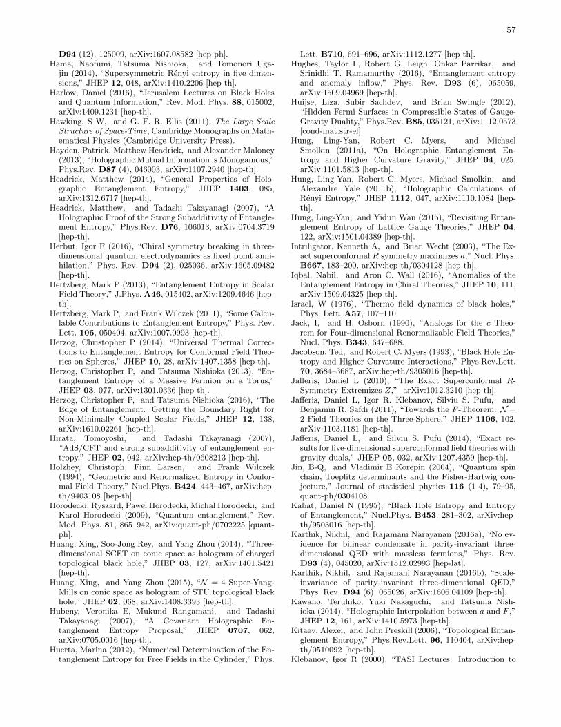
57

D94 (12), 125009, arXiv:1607.08582 [hep-ph].Hama, Naofumi, Tatsuma Nishioka, and Tomonori Uga-

jin (2014), “Supersymmetric Renyi entropy in five dimen-sions,” JHEP 12, 048, arXiv:1410.2206 [hep-th].

Harlow, Daniel (2016), “Jerusalem Lectures on Black Holesand Quantum Information,” Rev. Mod. Phys. 88, 015002,arXiv:1409.1231 [hep-th].

Hawking, S W, and G. F. R. Ellis (2011), The Large ScaleStructure of Space-Time, Cambridge Monographs on Math-ematical Physics (Cambridge University Press).

Hayden, Patrick, Matthew Headrick, and Alexander Maloney(2013), “Holographic Mutual Information is Monogamous,”Phys.Rev. D87 (4), 046003, arXiv:1107.2940 [hep-th].

Headrick, Matthew (2014), “General Properties of Holo-graphic Entanglement Entropy,” JHEP 1403, 085,arXiv:1312.6717 [hep-th].

Headrick, Matthew, and Tadashi Takayanagi (2007), “AHolographic Proof of the Strong Subadditivity of Entangle-ment Entropy,” Phys.Rev. D76, 106013, arXiv:0704.3719[hep-th].

Herbut, Igor F (2016), “Chiral symmetry breaking in three-dimensional quantum electrodynamics as fixed point anni-hilation,” Phys. Rev. D94 (2), 025036, arXiv:1605.09482[hep-th].

Hertzberg, Mark P (2013), “Entanglement Entropy in ScalarField Theory,” J.Phys. A46, 015402, arXiv:1209.4646 [hep-th].

Hertzberg, Mark P, and Frank Wilczek (2011), “Some Calcu-lable Contributions to Entanglement Entropy,” Phys. Rev.Lett. 106, 050404, arXiv:1007.0993 [hep-th].

Herzog, Christopher P (2014), “Universal Thermal Correc-tions to Entanglement Entropy for Conformal Field Theo-ries on Spheres,” JHEP 10, 28, arXiv:1407.1358 [hep-th].

Herzog, Christopher P, and Tatsuma Nishioka (2013), “En-tanglement Entropy of a Massive Fermion on a Torus,”JHEP 03, 077, arXiv:1301.0336 [hep-th].

Herzog, Christopher P, and Tatsuma Nishioka (2016), “TheEdge of Entanglement: Getting the Boundary Right forNon-Minimally Coupled Scalar Fields,” JHEP 12, 138,arXiv:1610.02261 [hep-th].

Hirata, Tomoyoshi, and Tadashi Takayanagi (2007),“AdS/CFT and strong subadditivity of entanglement en-tropy,” JHEP 02, 042, arXiv:hep-th/0608213 [hep-th].

Holzhey, Christoph, Finn Larsen, and Frank Wilczek(1994), “Geometric and Renormalized Entropy in Confor-mal Field Theory,” Nucl.Phys. B424, 443–467, arXiv:hep-th/9403108 [hep-th].

Horodecki, Ryszard, Pawel Horodecki, Michal Horodecki, andKarol Horodecki (2009), “Quantum entanglement,” Rev.Mod. Phys. 81, 865–942, arXiv:quant-ph/0702225 [quant-ph].

Huang, Xing, Soo-Jong Rey, and Yang Zhou (2014), “Three-dimensional SCFT on conic space as hologram of chargedtopological black hole,” JHEP 03, 127, arXiv:1401.5421[hep-th].

Huang, Xing, and Yang Zhou (2015), “N = 4 Super-Yang-Mills on conic space as hologram of STU topological blackhole,” JHEP 02, 068, arXiv:1408.3393 [hep-th].

Hubeny, Veronika E, Mukund Rangamani, and TadashiTakayanagi (2007), “A Covariant Holographic En-tanglement Entropy Proposal,” JHEP 0707, 062,arXiv:0705.0016 [hep-th].

Huerta, Marina (2012), “Numerical Determination of the En-tanglement Entropy for Free Fields in the Cylinder,” Phys.

Lett. B710, 691–696, arXiv:1112.1277 [hep-th].Hughes, Taylor L, Robert G. Leigh, Onkar Parrikar, and

Srinidhi T. Ramamurthy (2016), “Entanglement entropyand anomaly inflow,” Phys. Rev. D93 (6), 065059,arXiv:1509.04969 [hep-th].

Huijse, Liza, Subir Sachdev, and Brian Swingle (2012),“Hidden Fermi Surfaces in Compressible States of Gauge-Gravity Duality,” Phys.Rev. B85, 035121, arXiv:1112.0573[cond-mat.str-el].

Hung, Ling-Yan, Robert C. Myers, and MichaelSmolkin (2011a), “On Holographic Entanglement En-tropy and Higher Curvature Gravity,” JHEP 04, 025,arXiv:1101.5813 [hep-th].

Hung, Ling-Yan, Robert C. Myers, Michael Smolkin, andAlexandre Yale (2011b), “Holographic Calculations ofRenyi Entropy,” JHEP 1112, 047, arXiv:1110.1084 [hep-th].

Hung, Ling-Yan, and Yidun Wan (2015), “Revisiting Entan-glement Entropy of Lattice Gauge Theories,” JHEP 04,122, arXiv:1501.04389 [hep-th].

Intriligator, Kenneth A, and Brian Wecht (2003), “The Ex-act superconformal R symmetry maximizes a,” Nucl. Phys.B667, 183–200, arXiv:hep-th/0304128 [hep-th].

Iqbal, Nabil, and Aron C. Wall (2016), “Anomalies of theEntanglement Entropy in Chiral Theories,” JHEP 10, 111,arXiv:1509.04325 [hep-th].

Israel, W (1976), “Thermo field dynamics of black holes,”Phys. Lett. A57, 107–110.

Jack, I, and H. Osborn (1990), “Analogs for the c Theo-rem for Four-dimensional Renormalizable Field Theories,”Nucl. Phys. B343, 647–688.

Jacobson, Ted, and Robert C. Myers (1993), “Black Hole En-tropy and Higher Curvature Interactions,” Phys.Rev.Lett.70, 3684–3687, arXiv:hep-th/9305016 [hep-th].

Jafferis, Daniel L (2010), “The Exact Superconformal R-Symmetry Extremizes Z,” arXiv:1012.3210 [hep-th].

Jafferis, Daniel L, Igor R. Klebanov, Silviu S. Pufu, andBenjamin R. Safdi (2011), “Towards the F -Theorem: N =2 Field Theories on the Three-Sphere,” JHEP 1106, 102,arXiv:1103.1181 [hep-th].

Jafferis, Daniel L, and Silviu S. Pufu (2014), “Exact re-sults for five-dimensional superconformal field theories withgravity duals,” JHEP 05, 032, arXiv:1207.4359 [hep-th].

Jin, B-Q, and Vladimir E Korepin (2004), “Quantum spinchain, Toeplitz determinants and the Fisher-Hartwig con-jecture,” Journal of statistical physics 116 (1-4), 79–95,quant-ph/0304108.

Kabat, Daniel N (1995), “Black Hole Entropy and Entropyof Entanglement,” Nucl.Phys. B453, 281–302, arXiv:hep-th/9503016 [hep-th].

Karthik, Nikhil, and Rajamani Narayanan (2016a), “No ev-idence for bilinear condensate in parity-invariant three-dimensional QED with massless fermions,” Phys. Rev.D93 (4), 045020, arXiv:1512.02993 [hep-lat].

Karthik, Nikhil, and Rajamani Narayanan (2016b), “Scale-invariance of parity-invariant three-dimensional QED,”Phys. Rev. D94 (6), 065026, arXiv:1606.04109 [hep-th].

Kawano, Teruhiko, Yuki Nakaguchi, and Tatsuma Nish-ioka (2014), “Holographic Interpolation between a and F ,”JHEP 12, 161, arXiv:1410.5973 [hep-th].

Kitaev, Alexei, and John Preskill (2006), “Topological Entan-glement Entropy,” Phys.Rev.Lett. 96, 110404, arXiv:hep-th/0510092 [hep-th].

Klebanov, Igor R (2000), “TASI Lectures: Introduction to

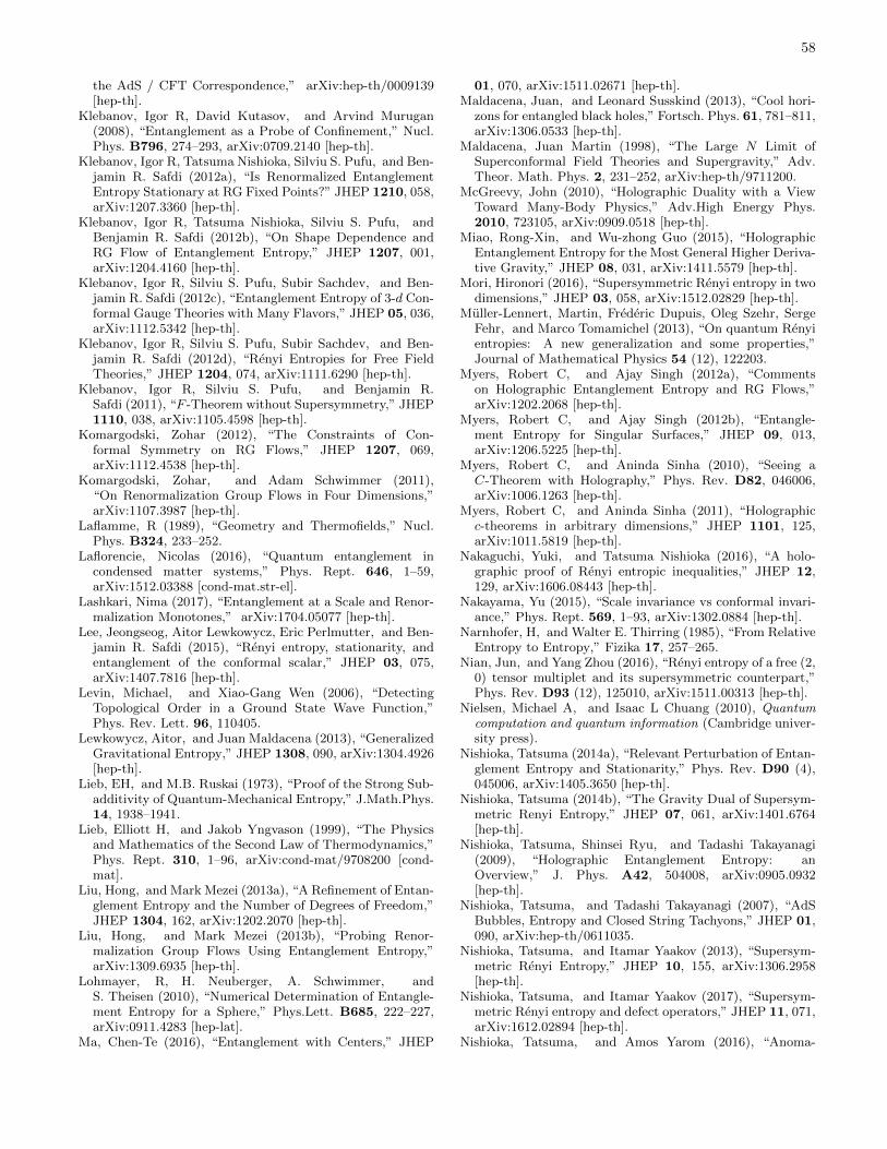
58

the AdS / CFT Correspondence,” arXiv:hep-th/0009139[hep-th].

Klebanov, Igor R, David Kutasov, and Arvind Murugan(2008), “Entanglement as a Probe of Confinement,” Nucl.Phys. B796, 274–293, arXiv:0709.2140 [hep-th].

Klebanov, Igor R, Tatsuma Nishioka, Silviu S. Pufu, and Ben-jamin R. Safdi (2012a), “Is Renormalized EntanglementEntropy Stationary at RG Fixed Points?” JHEP 1210, 058,arXiv:1207.3360 [hep-th].

Klebanov, Igor R, Tatsuma Nishioka, Silviu S. Pufu, andBenjamin R. Safdi (2012b), “On Shape Dependence andRG Flow of Entanglement Entropy,” JHEP 1207, 001,arXiv:1204.4160 [hep-th].

Klebanov, Igor R, Silviu S. Pufu, Subir Sachdev, and Ben-jamin R. Safdi (2012c), “Entanglement Entropy of 3-d Con-formal Gauge Theories with Many Flavors,” JHEP 05, 036,arXiv:1112.5342 [hep-th].

Klebanov, Igor R, Silviu S. Pufu, Subir Sachdev, and Ben-jamin R. Safdi (2012d), “Renyi Entropies for Free FieldTheories,” JHEP 1204, 074, arXiv:1111.6290 [hep-th].

Klebanov, Igor R, Silviu S. Pufu, and Benjamin R.Safdi (2011), “F -Theorem without Supersymmetry,” JHEP1110, 038, arXiv:1105.4598 [hep-th].

Komargodski, Zohar (2012), “The Constraints of Con-formal Symmetry on RG Flows,” JHEP 1207, 069,arXiv:1112.4538 [hep-th].

Komargodski, Zohar, and Adam Schwimmer (2011),“On Renormalization Group Flows in Four Dimensions,”arXiv:1107.3987 [hep-th].

Laflamme, R (1989), “Geometry and Thermofields,” Nucl.Phys. B324, 233–252.

Laflorencie, Nicolas (2016), “Quantum entanglement incondensed matter systems,” Phys. Rept. 646, 1–59,arXiv:1512.03388 [cond-mat.str-el].

Lashkari, Nima (2017), “Entanglement at a Scale and Renor-malization Monotones,” arXiv:1704.05077 [hep-th].

Lee, Jeongseog, Aitor Lewkowycz, Eric Perlmutter, and Ben-jamin R. Safdi (2015), “Renyi entropy, stationarity, andentanglement of the conformal scalar,” JHEP 03, 075,arXiv:1407.7816 [hep-th].

Levin, Michael, and Xiao-Gang Wen (2006), “DetectingTopological Order in a Ground State Wave Function,”Phys. Rev. Lett. 96, 110405.

Lewkowycz, Aitor, and Juan Maldacena (2013), “GeneralizedGravitational Entropy,” JHEP 1308, 090, arXiv:1304.4926[hep-th].

Lieb, EH, and M.B. Ruskai (1973), “Proof of the Strong Sub-additivity of Quantum-Mechanical Entropy,” J.Math.Phys.14, 1938–1941.

Lieb, Elliott H, and Jakob Yngvason (1999), “The Physicsand Mathematics of the Second Law of Thermodynamics,”Phys. Rept. 310, 1–96, arXiv:cond-mat/9708200 [cond-mat].

Liu, Hong, and Mark Mezei (2013a), “A Refinement of Entan-glement Entropy and the Number of Degrees of Freedom,”JHEP 1304, 162, arXiv:1202.2070 [hep-th].

Liu, Hong, and Mark Mezei (2013b), “Probing Renor-malization Group Flows Using Entanglement Entropy,”arXiv:1309.6935 [hep-th].

Lohmayer, R, H. Neuberger, A. Schwimmer, andS. Theisen (2010), “Numerical Determination of Entangle-ment Entropy for a Sphere,” Phys.Lett. B685, 222–227,arXiv:0911.4283 [hep-lat].

Ma, Chen-Te (2016), “Entanglement with Centers,” JHEP

01, 070, arXiv:1511.02671 [hep-th].Maldacena, Juan, and Leonard Susskind (2013), “Cool hori-

zons for entangled black holes,” Fortsch. Phys. 61, 781–811,arXiv:1306.0533 [hep-th].

Maldacena, Juan Martin (1998), “The Large N Limit ofSuperconformal Field Theories and Supergravity,” Adv.Theor. Math. Phys. 2, 231–252, arXiv:hep-th/9711200.

McGreevy, John (2010), “Holographic Duality with a ViewToward Many-Body Physics,” Adv.High Energy Phys.2010, 723105, arXiv:0909.0518 [hep-th].

Miao, Rong-Xin, and Wu-zhong Guo (2015), “HolographicEntanglement Entropy for the Most General Higher Deriva-tive Gravity,” JHEP 08, 031, arXiv:1411.5579 [hep-th].

Mori, Hironori (2016), “Supersymmetric Renyi entropy in twodimensions,” JHEP 03, 058, arXiv:1512.02829 [hep-th].

Muller-Lennert, Martin, Frederic Dupuis, Oleg Szehr, SergeFehr, and Marco Tomamichel (2013), “On quantum Renyientropies: A new generalization and some properties,”Journal of Mathematical Physics 54 (12), 122203.

Myers, Robert C, and Ajay Singh (2012a), “Commentson Holographic Entanglement Entropy and RG Flows,”arXiv:1202.2068 [hep-th].

Myers, Robert C, and Ajay Singh (2012b), “Entangle-ment Entropy for Singular Surfaces,” JHEP 09, 013,arXiv:1206.5225 [hep-th].

Myers, Robert C, and Aninda Sinha (2010), “Seeing aC-Theorem with Holography,” Phys. Rev. D82, 046006,arXiv:1006.1263 [hep-th].

Myers, Robert C, and Aninda Sinha (2011), “Holographicc-theorems in arbitrary dimensions,” JHEP 1101, 125,arXiv:1011.5819 [hep-th].

Nakaguchi, Yuki, and Tatsuma Nishioka (2016), “A holo-graphic proof of Renyi entropic inequalities,” JHEP 12,129, arXiv:1606.08443 [hep-th].

Nakayama, Yu (2015), “Scale invariance vs conformal invari-ance,” Phys. Rept. 569, 1–93, arXiv:1302.0884 [hep-th].

Narnhofer, H, and Walter E. Thirring (1985), “From RelativeEntropy to Entropy,” Fizika 17, 257–265.

Nian, Jun, and Yang Zhou (2016), “Renyi entropy of a free (2,0) tensor multiplet and its supersymmetric counterpart,”Phys. Rev. D93 (12), 125010, arXiv:1511.00313 [hep-th].

Nielsen, Michael A, and Isaac L Chuang (2010), Quantumcomputation and quantum information (Cambridge univer-sity press).

Nishioka, Tatsuma (2014a), “Relevant Perturbation of Entan-glement Entropy and Stationarity,” Phys. Rev. D90 (4),045006, arXiv:1405.3650 [hep-th].

Nishioka, Tatsuma (2014b), “The Gravity Dual of Supersym-metric Renyi Entropy,” JHEP 07, 061, arXiv:1401.6764[hep-th].

Nishioka, Tatsuma, Shinsei Ryu, and Tadashi Takayanagi(2009), “Holographic Entanglement Entropy: anOverview,” J. Phys. A42, 504008, arXiv:0905.0932[hep-th].

Nishioka, Tatsuma, and Tadashi Takayanagi (2007), “AdSBubbles, Entropy and Closed String Tachyons,” JHEP 01,090, arXiv:hep-th/0611035.

Nishioka, Tatsuma, and Itamar Yaakov (2013), “Supersym-metric Renyi Entropy,” JHEP 10, 155, arXiv:1306.2958[hep-th].

Nishioka, Tatsuma, and Itamar Yaakov (2017), “Supersym-metric Renyi entropy and defect operators,” JHEP 11, 071,arXiv:1612.02894 [hep-th].

Nishioka, Tatsuma, and Amos Yarom (2016), “Anoma-

59

lies and Entanglement Entropy,” JHEP 03, 077,arXiv:1509.04288 [hep-th].

Nishioka, Tatsuma, and Kazuya Yonekura (2013), “On RGFlow of τRR for Supersymmetric Field Theories in Three-Dimensions,” JHEP 05, 165, arXiv:1303.1522 [hep-th].

Ogawa, Noriaki, Tadashi Takayanagi, and Tomonori Uga-jin (2012), “Holographic Fermi Surfaces and EntanglementEntropy,” JHEP 1201, 125, arXiv:1111.1023 [hep-th].

Ohmori, Kantaro, and Yuji Tachikawa (2015), “Physics atthe entangling surface,” J. Stat. Mech. 1504, P04010,arXiv:1406.4167 [hep-th].

Ohya, Masanori (2004), Quantum entropy and its use(Springer).

Osborn, H (1989), “Derivation of a Four-dimensional c The-orem,” Phys. Lett. B222, 97–102.

Osborn, H, and A.C. Petkou (1994), “Implications of Confor-mal Invariance in Field Theories for General Dimensions,”Annals Phys. 231, 311–362, arXiv:hep-th/9307010 [hep-th].

Pakman, Ari, and Andrei Parnachev (2008), “TopologicalEntanglement Entropy and Holography,” JHEP 07, 097,arXiv:0805.1891 [hep-th].

Perlmutter, Eric (2014), “A universal feature of CFT Renyientropy,” JHEP 03, 117, arXiv:1308.1083 [hep-th].

Peschel, I (2003), “Calculation of reduced density matricesfrom correlation functions,” J. Phys. A: Math. Gen. 36,L205–L208, cond-mat/0212631.

Peschel, Ingo, and Ming-Chiang Chung (1999), “Densitymatrices for a chain of oscillators,” Journal of PhysicsA: Mathematical and General 32 (48), 8419, cond-mat/9906224.

Peschel, Ingo, and Viktor Eisler (2009), “Reduced densitymatrices and entanglement entropy in free lattice mod-els,” Journal of Physics A: Mathematical and Theoretical42 (50), 504003.

Petkou, Anastasios C (1995), “CT and CJ up to next-to-leading order in 1/N in the conformally invariant O(N)vector model for 2 < d < 4,” Phys. Lett. B359, 101–107,arXiv:hep-th/9506116 [hep-th].

Polchinski, Joseph (1984), “Renormalization and EffectiveLagrangians,” Nucl. Phys. B231, 269–295.

Preskill, J (1997), “Lecture notes for ph219/cs219,” http:

//www.theory.caltech.edu/people/preskill/ph229/.Pretko, Michael (2018), “On the Entanglement Entropy

of Maxwell Theory: A Condensed Matter Perspective,”arXiv:1801.01158 [hep-th].

Pretko, Michael, and T. Senthil (2016), “Entanglement en-tropy of U(1) quantum spin liquids,” Phys. Rev. B94 (12),125112, arXiv:1510.03863 [cond-mat.str-el].

Pufu, Silviu S (2016), “The F -Theorem and F -Maximization,” arXiv:1608.02960 [hep-th].

Radicevic, Djordje (2014), “Notes on Entanglement inAbelian Gauge Theories,” arXiv:1404.1391 [hep-th].

Radicevic, Djordje (2016), “Entanglement in Weakly CoupledLattice Gauge Theories,” JHEP 04, 163, arXiv:1509.08478[hep-th].

Rangamani, Mukund, and Tadashi Takayanagi (2017),“Holographic Entanglement Entropy,” Lect. Notes Phys.931, pp.1–246, arXiv:1609.01287 [hep-th].

Renyi, Alfred (1961), “On measures of entropy and infor-mation,” in Fourth Berkeley Symposium on MathematicalStatistics and Probability, pp. 547–561.

Rosenhaus, Vladimir, and Michael Smolkin (2014), “Entan-glement Entropy: A Perturbative Calculation,” JHEP 12,

179, arXiv:1403.3733 [hep-th].Rosenhaus, Vladimir, and Michael Smolkin (2015), “En-

tanglement Entropy for Relevant and Geometric Pertur-bations,” JHEP 02, 015, arXiv:1410.6530 [hep-th].

Ryu, Shinsei, and Tadashi Takayanagi (2006a), “Aspectsof Holographic Entanglement Entropy,” JHEP 08, 045,arXiv:hep-th/0605073.

Ryu, Shinsei, and Tadashi Takayanagi (2006b), “HolographicDerivation of Entanglement Entropy from AdS/CFT,”Phys.Rev.Lett. 96, 181602, arXiv:hep-th/0603001 [hep-th].

Sachdev, Subir (1993), “Polylogarithm identities in a confor-mal field theory in three-dimensions,” Phys. Lett. B309,285–288, arXiv:hep-th/9305131 [hep-th].

Safdi, Benjamin R (2012), “Exact and Numerical Results onEntanglement Entropy in (5+1)-Dimensional CFT,” JHEP1212, 005, arXiv:1206.5025 [hep-th].

Solodukhin, Sergey N (2008), “Entanglement Entropy, Con-formal Invariance and Extrinsic Geometry,” Phys. Lett.B665, 305–309, arXiv:0802.3117 [hep-th].

Solodukhin, Sergey N (2011), “Entanglement Entropy ofBlack Holes,” Living Rev. Rel. 14, 8, arXiv:1104.3712 [hep-th].

Solodukhin, Sergey N (2013), “The a-theorem and entangle-ment entropy,” arXiv:1304.4411 [hep-th].

Soni, Ronak M, and Sandip P. Trivedi (2016), “Aspects ofEntanglement Entropy for Gauge Theories,” JHEP 01, 136,arXiv:1510.07455 [hep-th].

Srednicki, Mark (1993), “Entropy and Area,” Phys. Rev. Lett.71, 666–669, arXiv:hep-th/9303048.

Swingle, Brian (2012), “Entanglement Renormalization andHolography,” Phys. Rev. D86, 065007, arXiv:0905.1317[cond-mat.str-el].

Takayanagi, Tadashi (2012), “Entanglement Entropy froma Holographic Viewpoint,” Class.Quant.Grav. 29, 153001,arXiv:1204.2450 [gr-qc].

Taylor, Marika, and William Woodhead (2016a),“Renormalized entanglement entropy,” JHEP 08, 165,arXiv:1604.06808 [hep-th].

Taylor, Marika, and William Woodhead (2016b), “The holo-graphic F theorem,” arXiv:1604.06809 [hep-th].

Umegaki, Hisaharu, et al. (1962), “Conditional expectationin an operator algebra. IV. Entropy and information,” inKodai Mathematical Seminar Reports, Vol. 14 (Tokyo In-stitute of Technology, Department of Mathematics) pp. 59–85.

Van Acoleyen, Karel, Nick Bultinck, Jutho Haegeman,Michael Marien, Volkher B. Scholz, and Frank Verstraete(2016), “The entanglement of distillation for gauge theo-ries,” Phys. Rev. Lett. 117 (13), 131602, arXiv:1511.04369[quant-ph].

Van Raamsdonk, Mark (2009), “Comments on quantum grav-ity and entanglement,” arXiv:0907.2939 [hep-th].

Van Raamsdonk, Mark (2017), “Lectures on Gravity and En-tanglement,” in Proceedings, Theoretical Advanced StudyInstitute in Elementary Particle Physics: New Frontiers inFields and Strings (TASI 2015): Boulder, CO, USA, June1-26, 2015 , pp. 297–351, arXiv:1609.00026 [hep-th].

Vassilevich, D V (2003), “Heat Kernel Expansion:User’s Manual,” Phys. Rept. 388, 279–360, arXiv:hep-th/0306138.

Vedral, V (2002), “The role of relative entropy in quantuminformation theory,” Rev. Mod. Phys. 74, 197–234.

Vidal, G, J. I. Latorre, E Rico, and A. Kitaev (2003), “En-tanglement in quantum critical phenomena,” Phys. Rev.

60

Lett. 90, 227902, arXiv:quant-ph/0211074 [quant-ph].Wilde, Mark M, Andreas Winter, and Dong Yang (2013),

“Strong converse for the classical capacity of entanglement-breaking channels,” arXiv preprint arXiv:1306.1586.

Willett, Brian (2017), “Localization on three-dimensionalmanifolds,” J. Phys. A50 (44), 443006, arXiv:1608.02958[hep-th].

Wilson, K G, and John B. Kogut (1974), “The Renormal-ization group and the epsilon expansion,” Phys. Rept. 12,75–200.

Witten, Edward (1998), “Anti-de Sitter Space and Holog-raphy,” Adv. Theor. Math. Phys. 2, 253–291, arXiv:hep-th/9802150.

Wolf, Michael M (2006), “Violation of the Entropic Area Lawfor Fermions,” Phys.Rev.Lett. 96, 010404, arXiv:quant-ph/0503219 [quant-ph].

Wolf, Michael M, Frank Verstraete, Matthew B Hastings, andJ Ignacio Cirac (2008), “Area laws in quantum systems:mutual information and correlations,” Physical review let-ters 100 (7), 070502.

Yankielowicz, Shimon, and Yang Zhou (2017), “Supersym-metric Renyi entropy and Anomalies in 6d (1,0) SCFTs,”JHEP 04, 128, arXiv:1702.03518 [hep-th].

Yao, Hong, and Xiao-Liang Qi (2010), “Entanglement en-tropy and entanglement spectrum of the Kitaev model,”Phys. Rev. Lett. 105 (8), 080501, arXiv:1001.1165 [cond-mat.str-el].

Yonekura, Kazuya (2013), “Perturbative c-theorem in d-dimensions,” JHEP 04, 011, arXiv:1212.3028 [hep-th].

Zamolodchikov, AB (1986), “Irreversibility of the Flux of theRenormalization Group in a 2D Field Theory,” JETP Lett.43, 730–732.

Zhou, Yang (2015), “Universal Features of Four-DimensionalSuperconformal Field Theory on Conic Space,” JHEP 08,052, arXiv:1506.06512 [hep-th].

Zhou, Yang (2016), “Supersymmetric Renyi entropy and Weylanomalies in six-dimensional (2,0) theories,” JHEP 06, 064,arXiv:1512.03008 [hep-th].

Zyczkowski, Karol (2003), “Renyi extrapolation of Shannonentropy,” Open Systems & Information Dynamics 10 (03),297–310.