Task Partitioning and Mapping to...

Lecture 7: Task Partitioning

and Mapping to Processes

Shantanu Dutt

ECE Dept., UIC

Acknowledgements

Adapted from:

• Chapter 3 slides, by A. Grama, of the text: Principles of Parallel Algorithm Design by Ananth Grama, Anshul Gupta, George Karypis, and Vipin Kumar

• CS 267, Dense Linear Algebra: Parallel Gaussian Elimination, James Demmel, www.cs.berkeley.edu/~demmel/cs267_Spr07

Overview: Algorithms and Concurrency

• Introduction to Parallel Algorithms ▫ Tasks and Decomposition ▫ Processes and Mapping ▫ Processes Versus Processors

• Decomposition Techniques ▫ Recursive Decomposition ▫ Recursive Decomposition ▫ Exploratory Decomposition ▫ Hybrid Decomposition

• Characteristics of Tasks and Interactions ▫ Task Generation, Granularity, and Context ▫ Characteristics of Task Interactions.

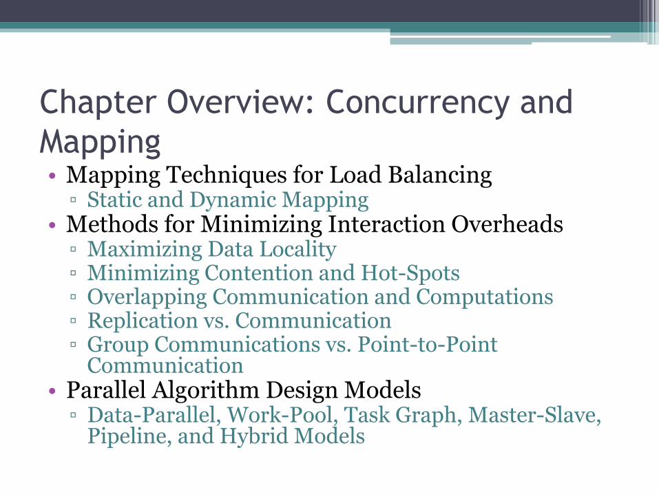
Chapter Overview: Concurrency and

Mapping • Mapping Techniques for Load Balancing ▫ Static and Dynamic Mapping

• Methods for Minimizing Interaction Overheads ▫ Maximizing Data Locality ▫ Minimizing Contention and Hot-Spots ▫ Overlapping Communication and Computations ▫ Replication vs. Communication ▫ Group Communications vs. Point-to-Point

Communication • Parallel Algorithm Design Models ▫ Data-Parallel, Work-Pool, Task Graph, Master-Slave,

Pipeline, and Hybrid Models

Preliminaries: Decomposition, Tasks,

and Dependency Graphs

• The first step in developing a parallel algorithm is to decompose the problem into tasks that can be executed concurrently

• A given problem may be decomposed into tasks in many different ways.

• Tasks may be of same, different, or even indeterminate sizes.

• A decomposition can be illustrated in the form of a directed graph with nodes corresponding to tasks and edges indicating that the result of one task is required for processing the next. Such a graph is called a task dependency graph.

Example: Multiplying a Dense Matrix with a Vector

Computation of each element of output vector y is independent of other

elements. Based on this, a dense matrix-vector product can be decomposed

into n tasks. The figure highlights the portion of the matrix and vector accessed

by Task 1.

Observations: While tasks share data (namely, the vector b ), they do not have

any control dependencies - i.e., no task needs to wait for the (partial) completion

of any other. All tasks are of the same size in terms of number of operations. Is

this the maximum number of tasks we could decompose this problem into?

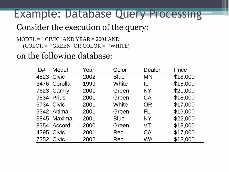
Example: Database Query Processing Consider the execution of the query:

MODEL = ``CIVIC'' AND YEAR = 2001 AND

(COLOR = ``GREEN'' OR COLOR = ``WHITE)

on the following database:

ID# Model Year Color Dealer Price

4523 Civic 2002 Blue MN $18,000

3476 Corolla 1999 White IL $15,000

7623 Camry 2001 Green NY $21,000

9834 Prius 2001 Green CA $18,000

6734 Civic 2001 White OR $17,000

5342 Altima 2001 Green FL $19,000

3845 Maxima 2001 Blue NY $22,000

8354 Accord 2000 Green VT $18,000

4395 Civic 2001 Red CA $17,000

7352 Civic 2002 Red WA $18,000

Example: Database Query Processing

The execution of the query can be divided into subtasks in various ways. Each task can be thought of as generating an intermediate table of entries that satisfy a particular clause.

Decomposing the given query into a number of tasks.

Edges in this graph denote that the output of one task

is needed to accomplish the next.

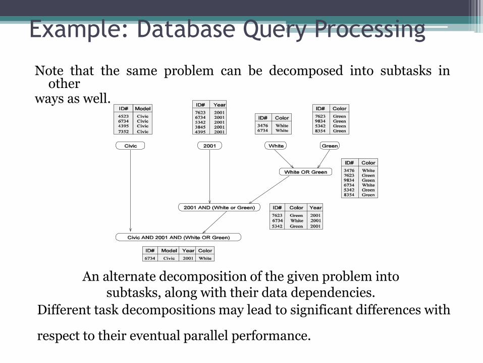
Example: Database Query Processing

Note that the same problem can be decomposed into subtasks in other

ways as well.

An alternate decomposition of the given problem into subtasks, along with their data dependencies.

Different task decompositions may lead to significant differences with

respect to their eventual parallel performance.

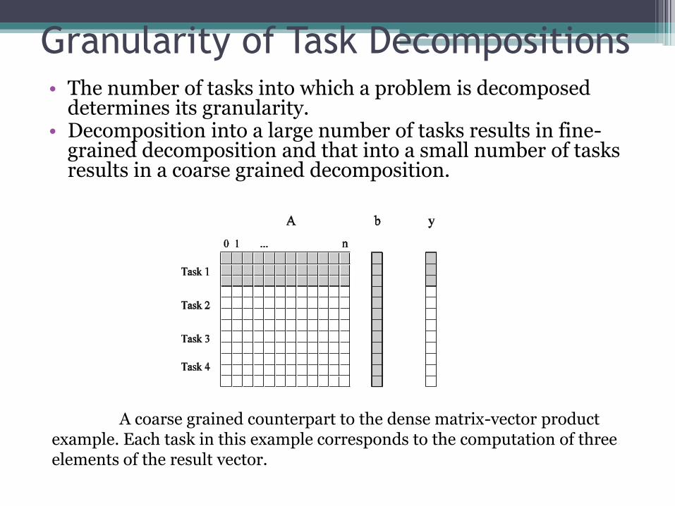
Granularity of Task Decompositions • The number of tasks into which a problem is decomposed

determines its granularity. • Decomposition into a large number of tasks results in fine-

grained decomposition and that into a small number of tasks results in a coarse grained decomposition.

A coarse grained counterpart to the dense matrix-vector product example. Each task in this example corresponds to the computation of three elements of the result vector.

Degree of Concurrency

• The number of tasks that can be executed in parallel is the degree of concurrency of a decomposition.

• Since the number of tasks that can be executed in parallel may change over program execution, the maximum degree of concurrency is the maximum number of such tasks at any point during execution. What is the maximum degree of concurrency of the database query examples?

• The average degree of concurrency is the average number of tasks that can be processed in parallel over the execution of the program. Assuming that each tasks in the database example takes identical processing time, what is the average degree of concurrency in each decomposition?

• The degree of concurrency increases as the decomposition becomes finer in granularity and vice versa.

Critical Path Length

• A directed path in the task dependency graph represents a sequence of tasks that must be processed one after the other.

• The longest such path determines the shortest time in which the program can be executed in parallel.

• The length of the longest path in a task dependency graph is called the critical path length.

Critical Path Length Consider the task dependency graphs of the two database query decompositions:

What are the critical path lengths for the two task dependency graphs?

If each task takes 10 time units, what is the shortest parallel execution time

for each decomposition? How many processors are needed in each case to

achieve this minimum parallel execution time? What is the maximum

degree of concurrency?

Limits on Parallel Performance

• It would appear that the parallel time can be made arbitrarily small by making the decomposition finer in granularity.

• There is an inherent bound on how fine the granularity of a computation can be. For example, in the case of multiplying a dense matrix with a vector, there can be no more than (n2) concurrent tasks.

• Concurrent tasks may also have to exchange data with other tasks. This results in communication overhead. The tradeoff between the granularity of a decomposition and associated overheads often determines performance bounds.

Task Interaction Graphs

• Subtasks generally exchange data with others in a decomposition. For example, even in the trivial decomposition of the dense matrix-vector product, if the vector is not replicated across all tasks, they will have to communicate elements of the vector.

• The graph of tasks (nodes) and their interactions/data exchange (edges) is referred to as a task interaction graph.

• Note that task interaction graphs represent data dependencies, whereas task dependency graphs represent control dependencies.

Task Interaction Graphs: An Example

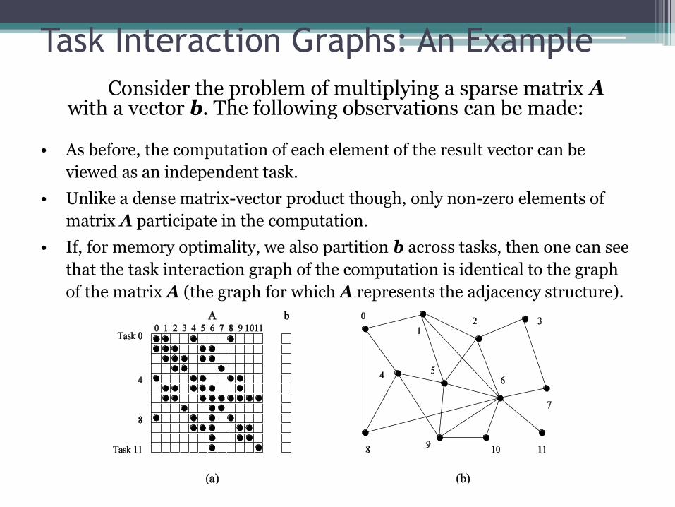
Consider the problem of multiplying a sparse matrix A with a vector b. The following observations can be made:

• As before, the computation of each element of the result vector can be

viewed as an independent task.

• Unlike a dense matrix-vector product though, only non-zero elements of

matrix A participate in the computation.

• If, for memory optimality, we also partition b across tasks, then one can see

that the task interaction graph of the computation is identical to the graph

of the matrix A (the graph for which A represents the adjacency structure).

Task Interaction Graphs, Granularity,

and Communication In general, if the granularity of a decomposition is finer,

the associated overhead (as a ratio of useful work assocaited with a task) increases.

Example: Consider the sparse matrix-vector product example from previous foil. Assume that each node takes unit time to process and each interaction (edge) causes an overhead of a unit time.

Viewing node 0 as an independent task involves a useful computation of one time unit and overhead (communication) of three time units.

Now, if we consider nodes 0, 4, and 8 as one task, then the task has useful computation totaling to three time units and communication corresponding to four time units (four edges). Clearly, this is a more favorable ratio than the former case.

Processes and Mapping

• In general, the number of tasks in a decomposition exceeds the number of processing elements available.

• For this reason, a parallel algorithm must also provide a mapping of tasks to processes.

Note: We refer to the mapping as being from tasks to processes, as opposed to processors. This is because typical programming APIs, as we shall see, do not allow easy binding of tasks to physical processors. Rather, we aggregate tasks into processes and rely on the system to map these processes to physical processors. We use processes, not in the UNIX sense of a process, rather, simply as a collection of tasks and associated data.


• Appropriate mapping of tasks to processes is critical to the parallel performance of an algorithm.

• Mappings are determined by both the task dependency and task interaction graphs.

• Task dependency graphs can be used to ensure that work is equally spread across all processes at any point (minimum idling and optimal load balance).

• Task interaction graphs can be used to make sure that processes need minimum interaction with other processes (minimum communication) for communication of input and intermediate data.


An appropriate mapping must minimize parallel execution time by:

• Mapping independent tasks to different processes.

• Assigning tasks on critical path to processes as soon as they

become available.

• Minimizing interaction between processes by mapping tasks with dense interactions to the same process.

Note: These criteria often conflict with each other. For example, a decomposition into one task (or no decomposition at all) minimizes interaction but does not result in a speedup at all! Can you think of other such conflicting cases?

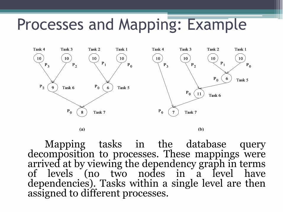
Processes and Mapping: Example

Mapping tasks in the database query decomposition to processes. These mappings were arrived at by viewing the dependency graph in terms of levels (no two nodes in a level have dependencies). Tasks within a single level are then assigned to different processes.

Decomposition Techniques

So how does one decompose a task into various subtasks?

While there is no single recipe that works for all

problems, we present a set of commonly used techniques that apply to broad classes of problems. These include:

• recursive decomposition • data decomposition • exploratory decomposition • speculative decomposition

Recursive Decomposition

• Generally suited to problems that are solved using the divide-and-conquer strategy.

• A given problem is first decomposed into a set of sub-problems.

• These sub-problems are recursively decomposed further until a desired granularity is reached.

Recursive Decomposition: Example A classic example of a divide-and-conquer algorithm on

which we can apply recursive decomposition is Quicksort.

In this example, once the list has been partitioned around the pivot, each sublist can be processed concurrently (i.e., each sublist represents an independent subtask). This can be repeated recursively.

Data Decomposition

• Identify the data on which computations are performed.

• Partition this data across various tasks.

• This partitioning induces a decomposition of the problem.

• Data can be partitioned in various ways - this critically impacts performance of a parallel algorithm.

Data Decomposition: Output Data

Decomposition • Often, each element of the output can be

computed independently of others (but simply as a function of the input).

• A partition of the output across tasks decomposes the problem naturally.

Output Data Decomposition: Example

Consider the problem of multiplying two n x n matrices A and B to yield matrix C. The output matrix C can be partitioned into four tasks as follows:

Task 1:

Task 2:

Task 3:

Task 4:


A partitioning of output data does not result in a unique decomposition into tasks. For example, for the same problem as in previus foil, with identical output data distribution, we can derive the following two (other) decompositions:

Decomposition I Decomposition II

Task 1: C1,1 = A1,1 B1,1

Task 2: C1,1 = C1,1 + A1,2 B2,1

Task 3: C1,2 = A1,1 B1,2

Task 4: C1,2 = C1,2 + A1,2 B2,2

Task 5: C2,1 = A2,1 B1,1

Task 6: C2,1 = C2,1 + A2,2 B2,1

Task 7: C2,2 = A2,1 B1,2

Task 8: C2,2 = C2,2 + A2,2 B2,2

Task 1: C1,1 = A1,1 B1,1

Task 2: C1,1 = C1,1 + A1,2 B2,1

Task 3: C1,2 = A1,2 B2,2

Task 4: C1,2 = C1,2 + A1,1 B1,2

Task 5: C2,1 = A2,2 B2,1

Task 6: C2,1 = C2,1 + A2,1 B1,1

Task 7: C2,2 = A2,1 B1,2

Task 8: C2,2 = C2,2 + A2,2 B2,2


Consider the problem of counting the instances of given itemsets in a database of transactions. In this case, the output (itemset frequencies) can be partitioned across tasks.


From the previous example, the following observations can be made:

• If the database of transactions is replicated across the processes, each task can be independently accomplished with no communication.

• If the database is partitioned across processes as well (for reasons of memory utilization), each task first computes partial counts. These counts are then aggregated at the appropriate task.

Input Data Partitioning

• Generally applicable if each output can be naturally computed or partially computed as a function of a subset of inputs (which may also then determine the input partitioning).

• In many cases, this is the only natural decomposition because the output is not clearly known a-priori (e.g., the problem of finding the minimum in a list, sorting a given list, etc.).

• A task is associated with each input data partition. The task performs as much of the computation with its part of the data. Subsequent processing combines these partial results.

Input Data Partitioning: Example

In the database counting example, the input (i.e., the transaction set) can be partitioned. This induces a task decomposition in which each task generates partial counts for all itemsets. These are combined subsequently for aggregate counts.

Partitioning Input and Output Data Often input and output data decomposition can be combined

for a higher degree of concurrency. For the itemset counting example, the transaction set (input) and itemset counts (output) can both be decomposed as follows:

Intermediate Data Partitioning

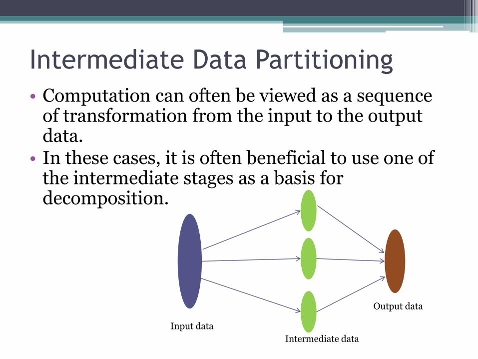
• Computation can often be viewed as a sequence of transformation from the input to the output data.

• In these cases, it is often beneficial to use one of the intermediate stages as a basis for decomposition.

Input data

Intermediate data

Output data

Intermediate Data Partitioning:

Example Let us revisit the example of dense matrix

multiplication. We first show how we can visualize this computation in terms of intermediate matrices D.

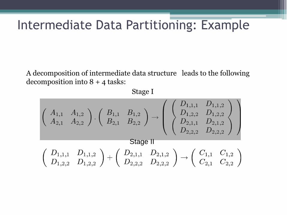
Intermediate Data Partitioning: Example

A decomposition of intermediate data structure leads to the following decomposition into 8 + 4 tasks:

Stage I

Stage II

The Owner Computes Rule

• The Owner Computes Rule generally states that the process assigned a particular data item is responsible for all computation associated with it—mainly applies to output data.

• In the case of input data decomposition, the owner computes rule imples that all computations that use the input data are performed by the process (this is generally not always applicable) .

• In the case of output data decomposition, the owner computes rule implies that the output is computed by the process to which the output data is assigned.

Exploratory Decomposition

• In many cases, the decomposition of the problem goes hand-in-hand with its execution.

• These problems typically involve the exploration (search) of a state space of solutions.

• Problems in this class include a variety of discrete optimization problems (0/1 integer programming, QAP, etc.), theorem proving, game playing, etc.

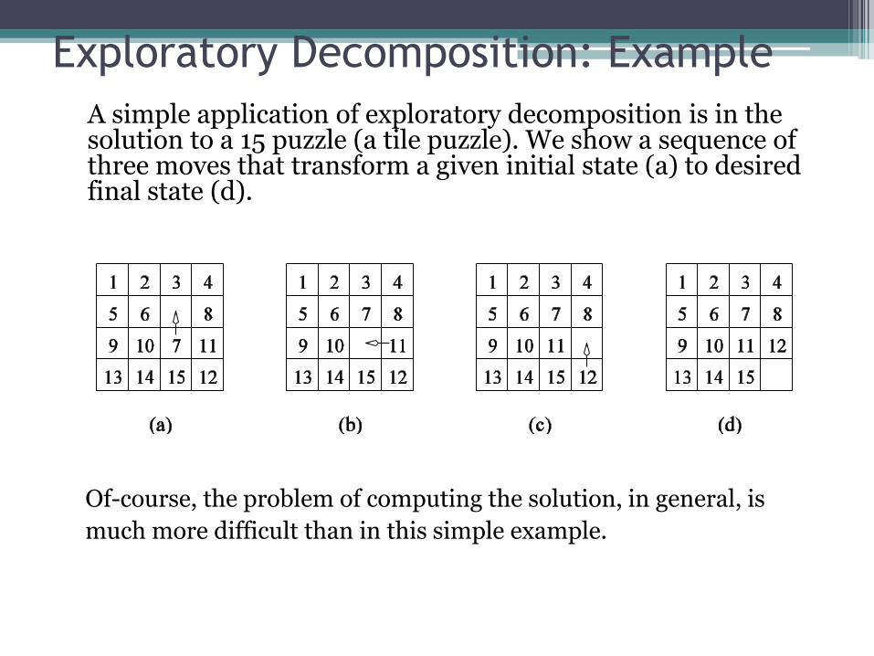
Exploratory Decomposition: Example

A simple application of exploratory decomposition is in the solution to a 15 puzzle (a tile puzzle). We show a sequence of three moves that transform a given initial state (a) to desired final state (d).

Of-course, the problem of computing the solution, in general, is

much more difficult than in this simple example.

Exploratory Decomposition: Example

The state space can be explored by generating various successor states of the current state and to view them as independent tasks.

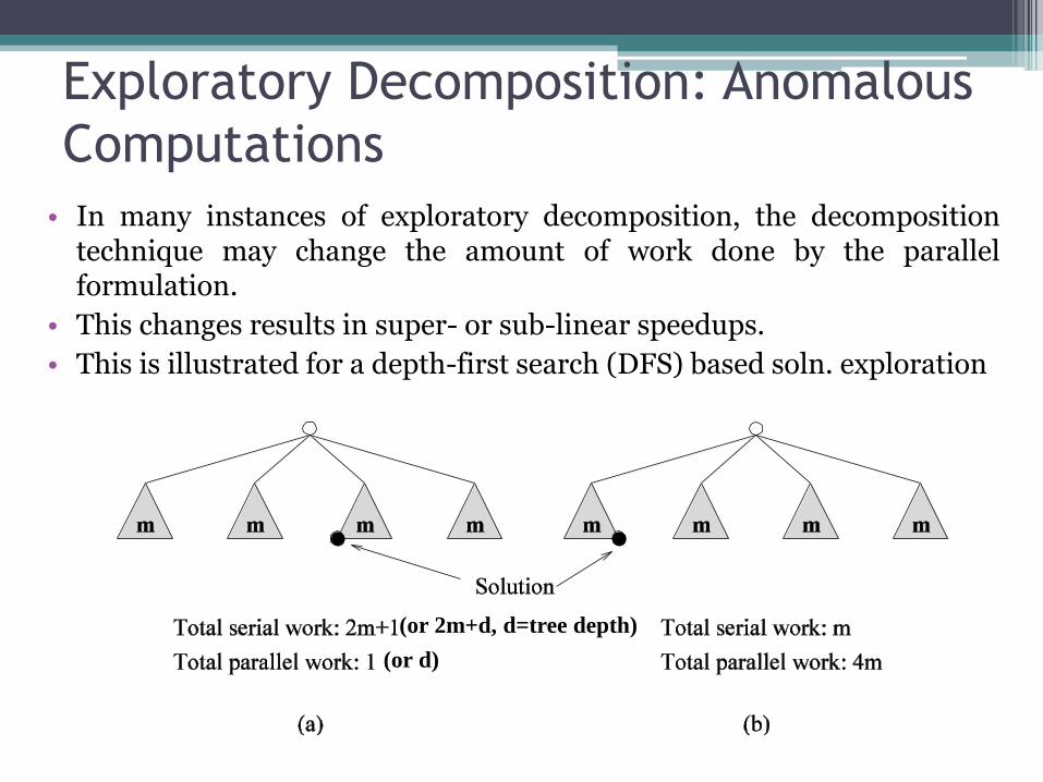
Exploratory Decomposition: Anomalous

Computations

• In many instances of exploratory decomposition, the decomposition technique may change the amount of work done by the parallel formulation.

• This changes results in super- or sub-linear speedups.

• This is illustrated for a depth-first search (DFS) based soln. exploration

(or 2m+d, d=tree depth)

(or d)

Speculative Decomposition

• In some applications, dependencies between tasks are not known a-priori.

• For such applications, it is impossible to identify independent tasks.

• There are generally two approaches to dealing with such applications: conservative approaches, which identify independent tasks only when they are guaranteed to not have dependencies, and, optimistic approaches, which schedule tasks even when they may potentially be erroneous.

• Conservative approaches may yield little concurrency and optimistic approaches may require roll-back mechanism in the case of an error.

Speculative Decomposition: Example

A classic example of speculative decomposition is in discrete event simulation.

• The central data structure in a discrete event simulation is a time-ordered event list.

• Events are extracted precisely in time order, processed, and if required, resulting events are inserted back into the event list.

• Consider your day today as a discrete event system - you get up, get ready, drive to work, work, eat lunch, work some more, drive back, eat dinner, and sleep.

• Each of these events may be processed independently, however, in driving to work, you might meet with an unfortunate accident and not get to work at all.

• Therefore, an optimistic scheduling of other events will have to be rolled back.

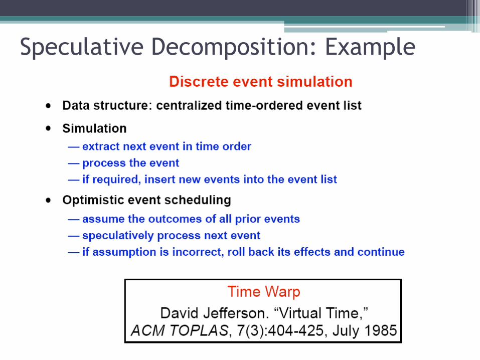
Speculative Decomposition: Example

Hybrid Decompositions

Often, a mix of decomposition techniques is necessary for

decomposing a problem. Consider the following examples:

• In quicksort, recursive decomposition alone limits concurrency (Why?). A

mix of data and recursive decompositions is more desirable.

• In discrete event simulation, there might be concurrency in task

processing. A mix of speculative decomposition and data decomposition

may work well.

• Even for simple problems like finding a minimum of a list of numbers, a

mix of data and recursive decomposition works well.

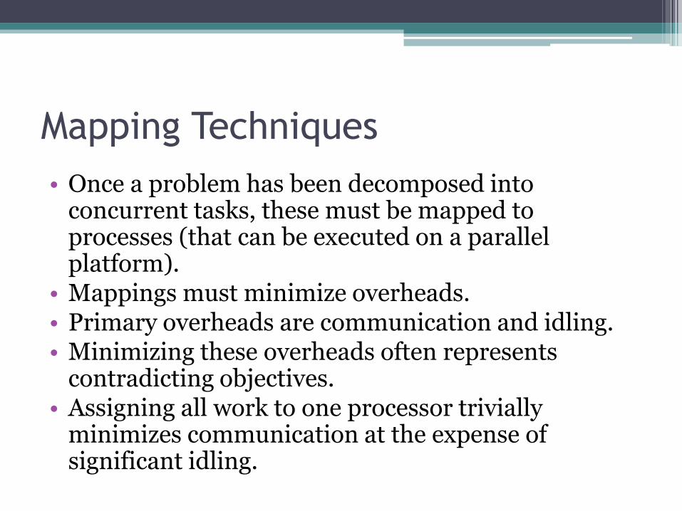
Mapping Techniques

• Once a problem has been decomposed into concurrent tasks, these must be mapped to processes (that can be executed on a parallel platform).

• Mappings must minimize overheads. • Primary overheads are communication and idling. • Minimizing these overheads often represents

contradicting objectives. • Assigning all work to one processor trivially

minimizes communication at the expense of significant idling.

Mapping Techniques for Minimum Idling

Mapping must simultaneously minimize idling and balance load.

Merely balancing load does not minimize idling.

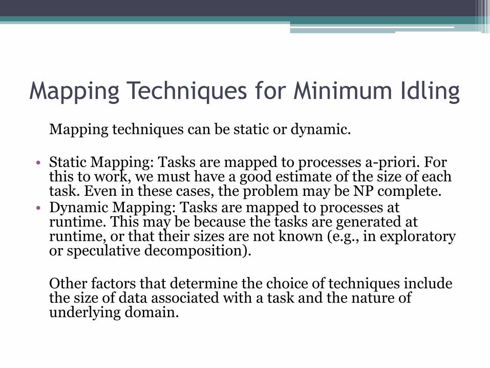
Mapping Techniques for Minimum Idling

Mapping techniques can be static or dynamic. • Static Mapping: Tasks are mapped to processes a-priori. For

this to work, we must have a good estimate of the size of each task. Even in these cases, the problem may be NP complete.

• Dynamic Mapping: Tasks are mapped to processes at runtime. This may be because the tasks are generated at runtime, or that their sizes are not known (e.g., in exploratory or speculative decomposition).

Other factors that determine the choice of techniques include

the size of data associated with a task and the nature of underlying domain.

Schemes for Static Mapping

• Mappings based on data partitioning.

• Mappings based on task graph partitioning.

• Hybrid mappings.

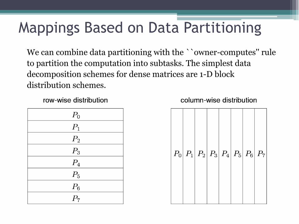
Mappings Based on Data Partitioning

We can combine data partitioning with the ``owner-computes'' rule

to partition the computation into subtasks. The simplest data

decomposition schemes for dense matrices are 1-D block

distribution schemes.

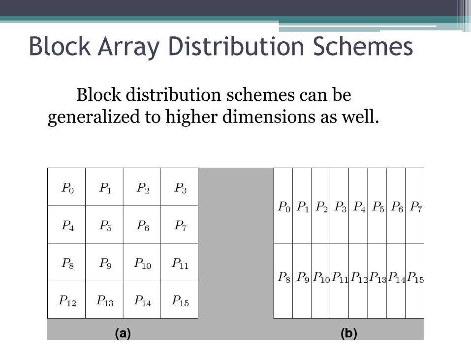
Block Array Distribution Schemes

Block distribution schemes can be generalized to higher dimensions as well.

Block Array Distribution Schemes:

Examples • For multiplying two dense matrices A and B, we can

partition the output matrix C using a block decomposition.

• For load balance, we give each task the same number of elements of C. (Note that each element of C corresponds to a single dot product.)

• The choice of precise decomposition (1-D or 2-D) is determined by the associated communication overhead.

• In general, higher dimension decomposition allows the use of larger number of processes.

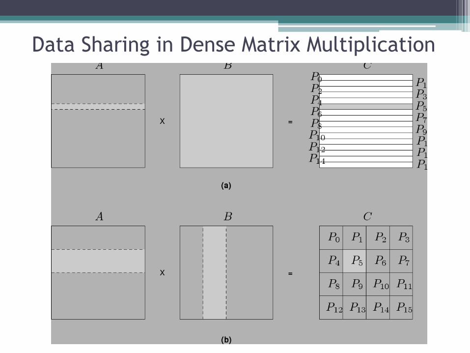
Data Sharing in Dense Matrix Multiplication

Cyclic and Block Cyclic Distributions

• If the amount of computation associated with data items varies by its position, a block decomposition may lead to significant load imbalances.

• A simple example of this is in LU decomposition (or Gaussian Elimination) of dense matrices.

• A cyclic block distribution can alleviate this problem

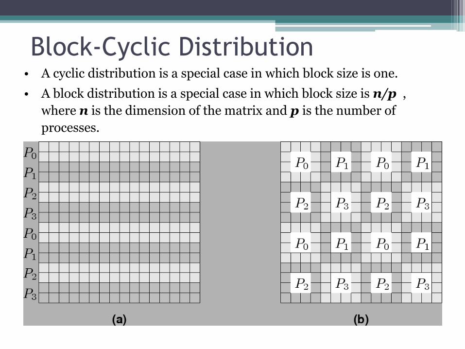
Block-Cyclic Distribution • A cyclic distribution is a special case in which block size is one.

• A block distribution is a special case in which block size is n/p ,

where n is the dimension of the matrix and p is the number of

processes.

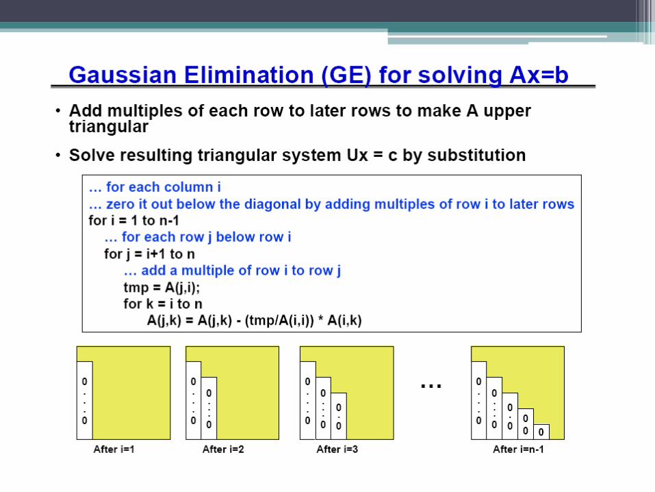
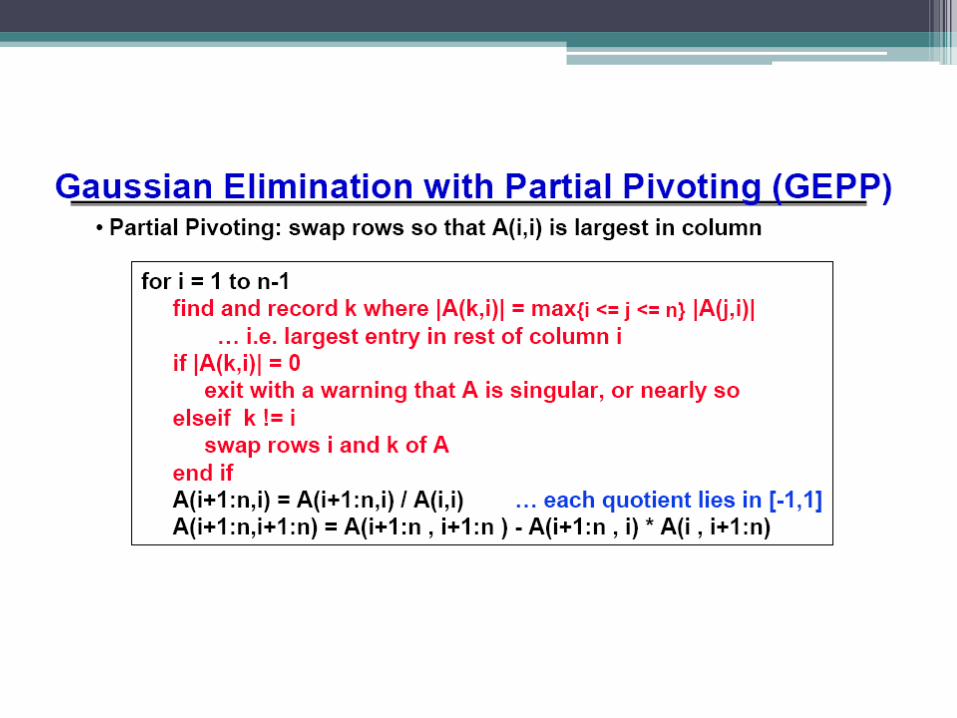
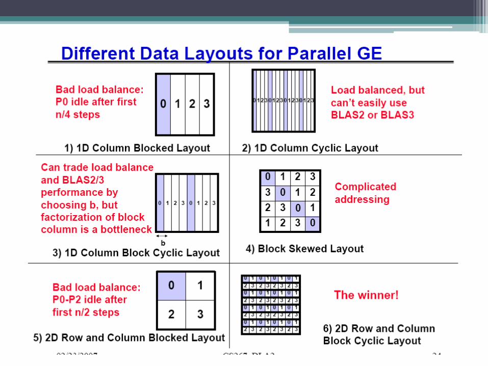
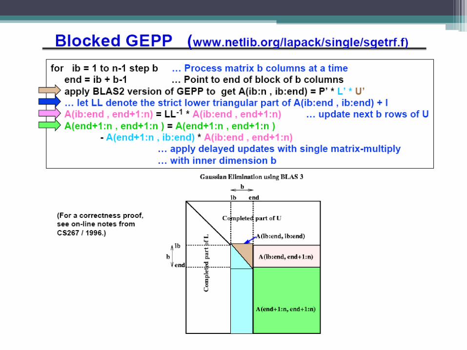
Block-Cyclic Distribution for Gaussian Elimination

The active part of the matrix in Gaussian Elimination changes.

By assigning blocks in a block-cyclic fashion, each processor receives

blocks from different parts of the matrix.

A[k,j]

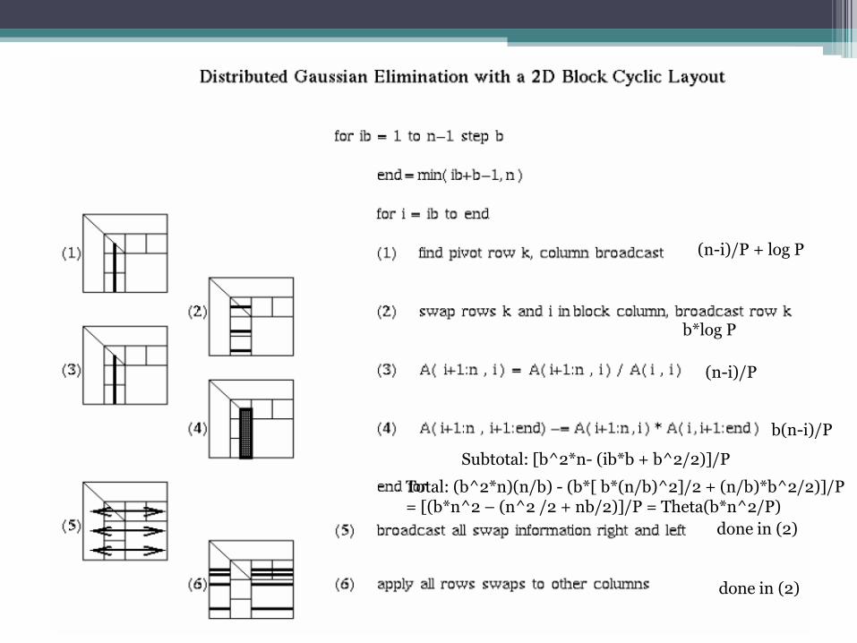
(n-i)/P + log P

b*log P

(n-i)/P

b(n-i)/P

done in (2)

done in (2)

Subtotal: [b^2*n- (ib*b + b^2/2)]/P

Total: (b^2*n)(n/b) - (b*[ b*(n/b)^2]/2 + (n/b)*b^2/2)]/P = [(b*n^2 – (n^2 /2 + nb/2)]/P = Theta(b*n^2/P)

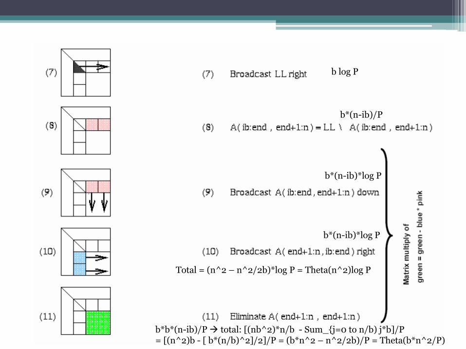
b log P

b*(n-ib)/P

b*(n-ib)*log P

b*(n-ib)*log P

b*b*(n-ib)/P total: [(nb^2)*n/b - Sum_{j=0 to n/b) j*b]/P = [(n^2)b - [ b*(n/b)^2]/2]/P = (b*n^2 – n^2/2b)/P = Theta(b*n^2/P)

Total = (n^2 – n^2/2b)*log P = Theta(n^2)log P

Block Cyclic Distributions

• Variation of the block distribution scheme that can be used to

alleviate the load-imbalance and idling problems.

• Partition an array into many more blocks than the number of

available processes.

• Blocks are assigned to processes in a round-robin manner so that

each process gets several non-adjacent blocks.

Graph Partitioning Dased Data

Decomposition • In case of sparse matrices, block decompositions are

more complex.

• Consider the problem of multiplying a sparse matrix with a vector.

• The graph of the matrix is a useful indicator of the work (number of nodes) and communication (the degree of each node).

• In this case, we would like to partition the graph so as to assign equal number of nodes to each process, while minimizing edge count of the graph partition.

Partitioning the Graph of Lake

Superior

Random Partitioning

Partitioning for minimum edge-cut.

Mappings Based on Task Paritioning

• Partitioning a given task-dependency graph across processes.

• Determining an optimal mapping for a general task-dependency graph is an NP-complete problem.

• Excellent heuristics exist for structured graphs.

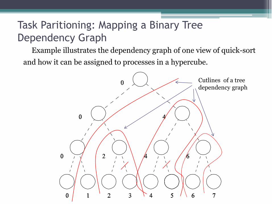
Task Paritioning: Mapping a Binary Tree

Dependency Graph Example illustrates the dependency graph of one view of quick-sort

and how it can be assigned to processes in a hypercube.

Cutlines of a tree dependency graph

Task Partioning: Mapping a Sparse Graph

Sparse graph for computing a sparse matrix-vector product and

its mapping.

17 items to be communicated

13 items to be communicated

Block Partitioning:

Graph Partitioning:

Schemes for Dynamic Mapping

• Dynamic mapping is sometimes also referred to as dynamic load balancing, since load balancing is the primary motivation for dynamic mapping.

• Dynamic mapping schemes can be centralized or distributed.

Centralized Dynamic Mapping

• Processes are designated as masters or slaves. • When a process runs out of work, it requests the

master for more work. • When the number of processes increases, the master

may become the bottleneck. • To alleviate this, a process may pick up a number of

tasks (a chunk) at one time. This is called Chunk scheduling.

• Selecting large chunk sizes may lead to significant load imbalances as well.

• A number of schemes have been used to gradually decrease chunk size as the computation progresses.

Distributed Dynamic Mapping

• Each process can send or receive work from other processes.

• This alleviates the bottleneck in centralized schemes.

• There are four critical questions: how are sensing and receiving processes paired together, who initiates work transfer, how much work is transferred, and when is a transfer triggered?

• Answers to these questions are generally application specific. We will look at some of these techniques later in this class.

Minimizing Interaction Overheads

• Maximize data locality: Where possible, reuse intermediate data.

• Minimize volume of data exchange: There is a cost associated with each word that is communicated. For this reason, we must minimize the volume of data communicated.

• Minimize frequency of interactions: There is a startup cost associated with each interaction. Therefore, try to merge multiple interactions to one, where possible.

• Minimize contention and hot-spots: Use decentralized techniques, replicate data where necessary.

Minimizing Interaction Overheads

(continued) • Overlapping computations with interactions:

Use non-blocking communications, multithreading, and prefetching to hide latencies.

• Replicating data or computations.

• Using group communications instead of point-to-point primitives.

• Overlap interactions with other interactions.

Parallel Algorithm Models An algorithm model is a way of structuring a parallel

algorithm by selecting a decomposition and mapping technique and applying the appropriate strategy to minimize interactions.

• Data Parallel Model: Tasks are statically (or semi-

statically) mapped to processes and each task performs similar operations on different data.

• Task Graph Model: Starting from a task dependency

graph, the interrelationships among the tasks are utilized to promote locality or to reduce interaction costs.

Parallel Algorithm Models (continued)

• Master-Slave Model: One or more processes generate work and allocate it to worker processes. This allocation may be static or dynamic.

• Pipeline / Producer-Comsumer Model: A stream of data is passed through a succession of processes, each of which perform some task on it.

• Hybrid Models: A hybrid model may be composed either of multiple models applied hierarchically on processor groups or multiple models applied sequentially to different phases of a parallel algorithm.

Characteristics of Tasks

Once a problem has been decomposed into independent tasks, the characteristics of these tasks critically impact choice and performance of parallel algorithms. Relevant task characteristics include:

• Task generation.

• Task sizes.

• Size of data associated with tasks.

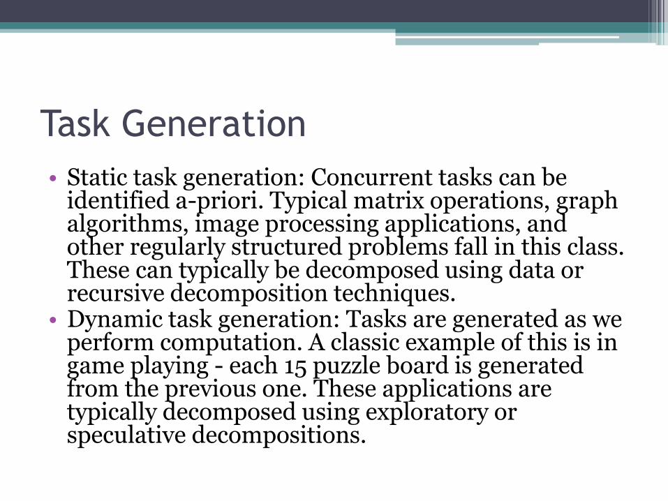
Task Generation

• Static task generation: Concurrent tasks can be identified a-priori. Typical matrix operations, graph algorithms, image processing applications, and other regularly structured problems fall in this class. These can typically be decomposed using data or recursive decomposition techniques.

• Dynamic task generation: Tasks are generated as we perform computation. A classic example of this is in game playing - each 15 puzzle board is generated from the previous one. These applications are typically decomposed using exploratory or speculative decompositions.

Task Sizes

• Task sizes may be uniform (i.e., all tasks are the same size) or non-uniform.

• Non-uniform task sizes may be such that they can be determined (or estimated) a-priori or not.

• Examples in the latter class include discrete optimization problems, in which it is difficult to estimate the effective size of a state space.

Size of Data Associated with Tasks

• The size of data associated with a task may be small or large when viewed in the context of the size of the task.

• A small context of a task implies that an algorithm can easily communicate this task to other processes dynamically (e.g., the 15 puzzle).

• A large context ties the task to a process, or alternately, an algorithm may attempt to reconstruct the context at another processes as opposed to communicating the context of the task (e.g., 0/1 integer programming).

Characteristics of Task Interactions

• Tasks may communicate with each other in various ways. The associated dichotomy is:

• Static interactions: The tasks and their interactions are known a-priori. These are relatively simpler to code into programs.

• Dynamic interactions: The timing or interacting tasks cannot be determined a-priori. These interactions are harder to code, especially, as we shall see, using message passing APIs.


• Regular interactions: There is a definite pattern (in the graph sense) to the interactions. These patterns can be exploited for efficient implementation.

• Irregular interactions: Interactions lack well-defined topologies.

Characteristics of Task Interactions:

Example A simple example of a regular static interaction pattern is in image

dithering. The underlying communication pattern is a structured (2-

D mesh) one as shown here:

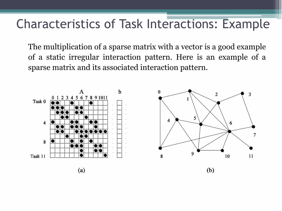
Characteristics of Task Interactions: Example

The multiplication of a sparse matrix with a vector is a good example

of a static irregular interaction pattern. Here is an example of a

sparse matrix and its associated interaction pattern.


• Interactions may be read-only or read-write.

• In read-only interactions, tasks just read data items associated with other tasks.

• In read-write interactions tasks read, as well as modily data items associated with other tasks.

• In general, read-write interactions are harder to code, since they require additional synchronization primitives.


• Interactions may be one-way or two-way.

• A one-way interaction can be initiated and accomplished by one of the two interacting tasks.

• A two-way interaction requires participation from both tasks involved in an interaction.

• One way interactions are somewhat harder to code in message passing APIs.

Task Partitioning and Mapping to...

Documents

Transcript of Task Partitioning and Mapping to...