Target Pricing: Demand-Side Versus Supply-Side …ywang195/research/TargetPricing.pdf · Target...

Target Pricing: Demand-Side Versus Supply-Side

Approaches

Hongmin Li

[email protected]

480-965-2232

Yimin Wang

yimin [email protected]

480-965-3888

Rui Yin

[email protected]

480-965-2998

Thomas J. Kull

[email protected]

480-965-6125

Thomas Y. Choi

[email protected]

480-965-6135

W.P. Carey School of Business

Arizona State University

Tempe, Arizona 85287, USA

Fax 480-965-8629


Approaches

Hongmin Li∗, Yimin Wanga, Rui Yinb, Thomas J. Kullc, Thomas Y. Choid

Arizona State University

Abstract

The practice of target pricing has been a key factor in the success of Japanese man-

ufacturers. In the more commonly-known demand-side approach, the target price for

the supplier equals the manufacturer’s market price less a percent margin for the man-

ufacturer but no cost-improvement expenses are shared. In the supply-side approach,

cost-improvement expenses are shared and the target price equals the supplier’s cost

plus a percent margin for the supplier. We find that sharing cost-reduction expenses

allows the manufacturer using the supply-side approach to attain competitive advan-

tage in the form of increased market share and higher profit, particularly in industries

where margins are thin and price sensitivities are high.

Keywords: Target Pricing, Cost-improvement Sharing, Competing Supply Chains,

Cournot Duopoly

∗ Corresponding author. W.P. Carey School of Business, Arizona State University, Tempe, AZ 85287

phone 480-965-2232, fax 480-965-8629, [email protected] [email protected]@[email protected]@asu.edu


Approaches

1 Introduction

Many manufactures have downsized supply base and have instituted long-term contracts

with their suppliers. In this setting, the practice of target pricing rather than competitive

pricing takes the center stage (Ellram 2006, Omar 1997, Cusumano and Takeishi 1991),

with manufacturers specifying prices to suppliers rather than suppliers submitting prices to

manufacturers. Although the target pricing practice is often observed in many different in-

dustries, its implementation often varies across manufacturers (Asanuma, 1985; Helper and

Sako, 1995; Liker et al. 1996). We identify two archetypes, terming one a demand-side (DS)

approach and the other a supply-side (SS) approach. In the DS approach, manufacturers

take the projected market price and work backwards to ascertain required prices for sub-

assemblies and individual parts. They then submit these target prices to their suppliers. In

the SS approach, manufacturers consider the supplier’s cost structure and apply a reasonable

supplier profit margin to determine the target price. Honda Motor Company, for example,

follows the SS approach by first learning extensively about a supplier’s cost structure and

then, based on this knowledge, specifying a target price to the supplier that combines both

the supplier’s cost and a percent margin (Liker and Choi 2004). Manufacturers may be

forced to practice the DS approach because they lack cost information about their suppliers.

As a result, they resort to the market price of their own product to determine what is a

reasonable target price for the components from the suppliers.

In this study, we examine how these two archetypes of target pricing can bring benefits or

detriments to manufacturers and suppliers. The DS approach uses demand-side information

and is based on the market price of a manufacturer’s product less the manufacturer’s desired

margin. Manufacturers using this approach allow suppliers to independently make cost

reductions. They generally do not share in the supplier’s cost-reduction expenses as they are

not actively involved in the production process of the suppliers and without such investment,

it is difficult to gain accurate knowledge of the supplier’s cost structure. For example, a

Honda supplier may present the“real” bill of material (BOM) cost only after it truly believes

Honda is there to help; before that, only a “guest” version of the cost book may be shown.

Hence, the DS approach can follow from manufacturers choosing not to invest in supplier

development, rather than favoring one approach over the other.

The advantage of the DS approach is that it assures manufacturer profit margins while

1

lowering relationship costs ( albeit often at the expense of lower supplier margins). On the

other hand, the SS approach focuses on supplier costs, with both parties seeking desired

margins through joint cost-reduction efforts (Handfield et al. 2004). The SS approach aims

to lower material costs at the expense of higher management costs and potentially lower

manufacturer margins, yet can result in overall supply chain benefits (Cooper and Yoshikawa,

1994). Although both approaches have context specific advantages, no previous studies have

analytically examined how the manufacturer-supplier joint improvement activities influence

the relative attractiveness of these two policies.

According to Ellram (2006), many Japanese manufacturers actually use both approaches

when determining a target price. They look to the market and establish the target price,

while comparing this target price against the cost breakdowns from the supplier side. How-

ever, many US-based manufacturers that are new to target pricing tend to take the market

side information and apply it as a target price to the supplier without considering supply-side

information. This is not surprising because much effort is required to gather information

from the supplier. In fact, the advantage of the DS approach is that it does not require

heavy investment in supplier development; marketing can determine the market price and

finance can work backwards to determine purchase prices. This approach is expedient and

requires less administrative cost. In effect, the DS approach is driven more by marketing

and finance, whereas the SS approach is driven more by operations and supply management.

For instance, to practice the SS approach, Honda sent a representative to a potential

parts supplier, Atlantic Tool and Die, to work on its production lines while learning about

this supplier’s capability and capacity (Liker and Choi, 2004). Honda took about one year

to learn what was possible at Atlantic. Honda’s final submitted target price was such that

Atlantic would have a small amount of profit and only through cost improvements could

Atlantic earn more profit. Honda in return was fully willing to assist Atlantic in improvement

efforts through Honda’s supplier development programs. In general, Honda will devote over

ten weeks of assistance at a supplier’s plant; an improvement effort that obviously requires a

high amount of Honda’s resources. Are such efforts worth the expense? Moreover, research

shows that manufacturers often turn to target pricing as competition intensifies (Ax et al.,

2008). Is this a good strategy?

Using an oligopoly model of multiple manufacturers each with a sole-source supplier, and

each adopting one of the two target pricing approaches, we characterize the equilibrium and

the optimal policy for each supply chain. We then focus on a duopoly situation in which

we contrast a DS model and a SS model in a Cournot competition. In addition, we also

examine the duopoly between two DS models, as well the duopoly between two SS models.

The Cournot competition model is common in the operations management literature when

2

competing supply chain structures are studied (e.g., Li, 2002; Wu and Chen, 2003; Gilbert

et al, 2006; Majumder and Srinivasan, 2008; Ha and Tong, 2008). In particular, the Cournot

competition model has often been used in a retail setting where retailers (or manufacturers)

compete for market share. Recent studies in this stream of literature have focused on the

role of information sharing (e.g., Li, 1985,2002; Zhang, 2002; Ha and Tong, 2008; Yao et

al., 2008) and channel coordination (e.g., Gupta and Loulou, 1998; Wu and Chen, 2003;

Narayanan et al., 2005).

Three recent papers are closely related to our research. Gilbert et al (2006) consider two

manufacturers sourcing from a common supplier. They find that outsourcing helps dampen

the competition between the manufacturers and reduces the over-investment for cost reduc-

tion. In addition, they consider the case when each manufacturer outsources to a sole-source

supplier and the suppliers do not directly compete. A supplier makes an investment in cost

reduction, announces the price, and then the manufacturer determines whether to make or

buy. Note that our focus is quite different from that of Gilbert et al (2006): Although we

also study the role of cost-reduction efforts between two competing supply chains, we focus

on cost-improvement investment sharing between supply chain members, while they focus

on the interaction between outsourcing and cost-reductions. Our study also complements

Majumder and Srinivasan (2008), who study a duopoly between two supply chains with

different structures. They incorporate scale economy to study the impact of competition on

wholesale prices and quantities. Ha and Tong (2008) study a similar duopoly structure as

this paper, but focus on the decision of information sharing between the two members in

each supply chain and consider the impact of contract types on the equilibrium outcome. We

build on this stream of literature and examine a duopoly between two supply chains with

the same sole-sourcing structure, but each with fundamentally different supplier develop-

ment strategies. This is reflected in the target pricing policies, as well as the manufacturer’s

behavior toward cost-reduction investment sharing. Recently, interest has grown in the lit-

erature regarding the manufacturer’s role in helping suppliers (e.g., Zhu et al., 2007; Babich,

2010; Wang et al, 2010), and our paper adds to that literature stream.

This paper contributes to the target pricing literature by contrasting the demand-side

approach and the supply-side approach; these two supply chain practices compete against

each other. In our model, we investigate the impact of joint manufacturer-supplier improve-

ment efforts on the equilibrium outcome. We find that, when the manufacturer in the SS

supply chain increases its share of cost-improvement expenses, it increases the SS supplier’s

incentive for cost improvement, but decreases the DS supplier’s cost-improvement effort.

By offering to engage in the supplier’s cost-improvement activity and share the cost, the

SS manufacturer increases its equilibrium market share. In addition, both the equilibrium

3

market price and the equilibrium transfer price in both supply chains (the price that each

manufacturer pays to its supplier) decrease monotonically with the SS manufacturer’s cost

share. For the SS supplier, this is offset by much-lowered cost. However, the DS supplier

may experience profit deterioration as a result of lower transfer price. Lastly, we explore the

optimal expense-sharing for the centralized supply chain and show that the manufacturer

shares more in the centralized solution than the decentralized solution.

To the best of our knowledge, this study is the first to systematize the anecdotal evidence

pertaining to target pricing and supplier improvement efforts.

The rest of the paper is organized as follows. In §2 we introduce the model setup, and we

fully characterize the manufacturer and the supplier’s optimal decision in §3. In §5 we study

the managerial implications of the joint supplier improvement effort. In §6, we explore how

various parameters affect the equilibrium solution using sensitivity analysis. We conclude in

§7. All proofs are contained in the Appendix.

2 The Model

We consider a single period oligopoy consisting of multiple supply chains. Each supply chain

has two members: a manufacturer and a supplier. Following previous literature and what

is observable in practice (Agndal and Nilsson, 2008; Lovejoy, 2010), the manufacturer sole-

sources a product from the supplier and then sells it to the end market. The manufacturers

engage in an oligopoly competition -the market price is identical for all manufacturers, but

the quantities sold by the manufacturers may differ due to the difference in costs. Within

each supply chain, the supplier and manufacturer play a sequential game. First, they form

an agreement on the transfer price scheme and the target price. Second, the supplier decides

the per-unit amount of cost-reduction. The supplier’s decision to invest in cost reduction

affects the production cost of the product, and, depending on which target price scheme

is used, the decision may affect the cost to the manufacturer. Third, the manufacturers

then sell the product to the same end market and form an oligopoly. The outcome is an

oligopoly equilibrium in which the manufacturer with the lower cost obtains a larger market

share. Note that each supplier sells to its respective manufacturer only and there is no direct

competition between the suppliers. Often there are suppliers in the same market but they do

not compete for the same contract. For example, Bridgestone supplies tires for one model,

and Michelin suppliers tires for another model-for each model they are sole-sourced and these

two companies are not in direct competition. Therefore, for our purpose, it is reasonable

to assume no direct competition between the suppliers for the component or service under

consideration.

4

Let there be a total of n manufacturers, among which J manufacturers adopt the SS

approach for determining the transfer price and K manufacturers adopt the DS approach.

Let the set S be the set of SS manufacturers (or suppliers) and let the set S be the set of

DS manufacturers.

Let qi denote the quantity supplied by manufacturer i (i = 1, 2, . . . , n) to the end market.

The total quantity of the product to the end market is therefore q =∑n

i=1 qi. The market

price is linear in the quantity supplied:

p = a − b

n∑

i=1

qi, (2.1)

where p is the market price, a represents the maximal willingness to pay, and b is the slope

of the (inverse) demand function. Manufacturers simultaneously determine their selling

quantities to the end market and each manufacturer receives a revenue of p · qi. Because

our model is a multi-stage sequential game, as described earlier, the improvement expenses

are sunk when the manufacturers make the decision on procurement quantities. Therefore,

the equilibrium quantities depend on the cost improvement only through the transfer prices.

That is, whether a manufacturer shares any of the expense for its supplier’s cost-reduction

initiative is irrelevant at this stage of decision making.

Within each supply chain i; where i = 1, 2, . . . , n; manufacturer i pays a linear, per-unit

target price wi to the supplier. As discussed in the introduction, we consider two alternative

approaches for setting the target price wi between a manufacturer and its supplier. In

the SS approach, the manufacturer pays the supplier according to a transfer price wj =

cej(1 + mj), j ∈ S where ce

j is the supplier j’s unit production cost and mj is a fixed percent

margin for the supplier. We do not consider the detailed negotiations of m and simply regard

m as exogenous. In the DS approach, the manufacturer pays the supplier a transfer price

wk = p(1− rk), k ∈ S where p is the Cournot equilibrium market price and rk is the desired

margin for the manufacturer.1

Suppliers may have incentives to reduce their production cost to maximize profit. Hence,

each supplier may decide, at its own discretion, the per-unit cost reduction amount (defined

as ei, for supplier i, i = 1, 2, . . . , n). We assume that supplier i will be able to achieve the

desired reduction in the per unit production cost of the supplier by ei.

cei = ci − ei.

1To be precise, the target price wi would also depend on the fraction of the component cost (procured

from the supplier) relative to the total cost of the final product. This can be easily incorporated in the model

by introducing a scaling parameter and will not affect any of the subsequent analysis.

5

where ci is the initial unit production cost and cei is the realized production cost for supplier i

after the cost reduction. The expense required to achieve the cost improvement is (1/2)µie2i ,

which is convex increasing in ei. The exact functional form of (1/2)µie2i is motivated by

the fact that the improvement effort has declining marginal returns. That is, it becomes

increasingly difficult to achieve further cost reductions (Bernstein and Kok, 2009). Such

convex functional form is also commonly used in the economics literature for analytical

tractability. The cost-improvement expense is assumed to be independent of the quantities

produced as we focus on process improvements in manufacturing. Note that we only consider

the benefit in the form of cost reduction. In addition, to focus on the difference between the

two supply chains and for simplicity, we do not consider the case where improvement effort

may result in a stochastic cost-reduction outcome, and we assume µi = µ, ∀i = 1, 2, . . . , n.

Consistent with industry practice (see Liker and Choi, 2004; Hartley and Choi, 1996), we

assume that the manufacturer in the SS supply chain shares a portion θj (0 ≤ θj ≤ 1,j ∈ S) of

the cost-improvement expenses incurred by the supplier. In contrast, we scale θk = 0, k ∈ S

for the DS supply chain, i.e., the manufacturer in the DS supply chain does not share the

improvement expenses incurred by the supplier. Although some DS manufacturers engage

in supplier development (e.g. short-term oriented kaizen blitz), the expense they incur

compared to the SS approach is much less and is assumed to be negligible for our comparative

study. Hereafter we refer to θi as the joint improvement share.

2.1 Problem Formulation

For notational clarity, we assume that the DS and SS chains are symmetric except for the

target pricing policies discussed above. In our model, the Cournot competition takes place

between the DS and SS supply chains, and performance comparisons are made at the supply

chain level. We have done additional analysis of the Cournot competition between two

same supply chains (i.e. two DS supply chains or two SS supply chains) and the details are

available upon request.

To formulate the problem, we describe the sequence of events.2 We assume that each

supply chain will determine its margins through negotiation (mj for the SS supply chain and

rk for the DS supply chain respectively). This agreement then forms a blanket contract for

future dealings. In modeling the sequential duopoly game, we treat mj and rk as exogenously

given. At the start of the game, the suppliers decide the amount of cost-reduction ei, recog-

nizing that their efforts will affect the manufacturers’s decision in production (procurement)

2Although we consider a single period simultaneous game, the sequence of events does matter in charac-

terizing optimal solutions.

6

quantities. Then the production cost cei is realized. Next, the manufacturers simultaneously

choose the optimal production quantity q = (q1, q2, . . . , qn) to maximize their own profits

based on the transfer prices. Note that we do not distinguish the procurement quantity from

the production or sales quantity because the market price is endogenous to the quantity sold

to the market.

We now describe the manufacturers’ and the suppliers’ objectives. The profit function

for manufacturer i is given by

ΠMi (qi) = (p − wi)qi −

1

2µθie

2i , (2.2)

where the reader will recall that p = a − b∑n

i=1 qi, θk = 0, k ∈ S and θj ≥ 0, j ∈ S. The

profit function for supplier i can be expressed as

ΠSi (ei) = (wi − ce

i )qi −1

2µ(1 − θi)e

2i . (2.3)

In (2.3), the first term is the supplier’s net profit before the cost reduction and cei is the

supplier’s unit production cost after the cost reduction. The second term is the expense of

making such cost reductions.

In summary, the DS and SS supply chains differ in two aspects. First, in the DS supply

chain the supplier assumes the entire expense of the cost reduction effort 12µe2

k, k ∈ S,

whereas in the SS supply chain the manufacturer shares a fraction θ of the supplier’s expenses.

Second, the target pricing policy differs between the two types of supply chains. As discussed

before, the DS supply chain adopts a demand-side policy, with wk = p(1 − rk), whereas the

SS supply chain adopts a supply-side policy, with wj = cej(1 + mj). We emphasize that

these two aspects are closely tied: The manufacturer in the DS chain is not actively involved

in supplier development and thus does not have good cost information about its supplier.

Consequently, it is forced to use the DS policy because a SS policy is not possible without

first hand information of supplier cost.

3 Characterization of Oligopoly Equilibrium

In this section, we analyze the optimal decision for each member in the supply chain. We

also examine the impact of the joint improvement expense sharing on each supplier’s cost-

reduction efforts and each supply chain’s profit.

In what follows, we solve the manufacturers’ oligopoly competition problem and derive

the equilibrium market price. The solution to this oligopoly equilibrium will facilitate the

7

characterization of the suppliers’ cost improvement problem. Substituting (2.1) into (2.2),

we have

ΠMi (qi) =

(

a − b

n∑

i=1

qi − wi

)

qi −1

2µθie

2i , i = 1, 2, . . . , n. (3.1)

Note again here the decisions on quantities (i.e., qi) and effort sharing (θi) are decoupled

due to the sequential game assumption. It is straightforward to verify that (3.1) is jointly

concave in qi, i = 1, 2, . . . , n and their optimal quantities are given by

q∗i =a +

∑nℓ=1 wℓ − (n + 1)wi

(n + 1)b, i = 1, 2, . . . , n. (3.2)

Substituting (3.2) into (2.1), we obtain the market equilibrium price

p∗ =a +

∑nℓ=1 wℓ

n + 1. (3.3)

Note that both the optimal production quantities q∗ and the market equilibrium price p∗

implicitly depend on the suppliers’ improvement effort.3 Substituting p∗ into (3.1), we can

simplify the manufacturers’ profit functions as:

ΠMi =

[a +∑n

ℓ=1 wℓ − (n + 1)wi]2

(n + 1)2b−

1

2θiµe2

i . (3.4)

Similarly, we simplify the suppliers’ profit functions by substituting p∗ into (2.3):

ΠSi = (wi − c + ei)

a +∑n

ℓ=1 wℓ − (n + 1)wi

(n + 1)b−

1

2(1 − θi)µe2

i , (3.5)

where we assume ci = c, i = 1, 2, . . . , n, i.e., the suppliers’ unit production costs in both

supply chains are identical before the improvement efforts.

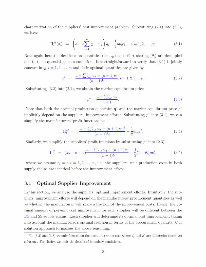
3.1 Optimal Supplier Improvement

In this section, we analyze the suppliers’ optimal improvement efforts. Intuitively, the sup-

pliers’ improvement efforts will depend on the manufacturers’ procurement quantities as well

as whether the manufacturer will share a fraction of the improvement costs. Hence, the op-

timal amount of per-unit cost improvement for each supplier will be different between the

DS and SS supply chains. Each supplier will determine its optimal cost improvement, taking

into account the manufacturer’s optimal reaction in terms of the procurement quantity. Our

solution approach formalizes the above reasoning.

3In (3.2) and (3.3) we only focused on the most interesting case where q∗i

and p∗ are all interior (positive)

solutions. For clarity, we omit the details of boundary conditions.

8

Proposition 1 In a quantity-competition oligopoly, the equilibrium market price is given by

p∗ =a + µbc

∑

j∈S Gj(1 − θj)/mj

n + 1 − K +∑

k∈S rk −∑

j∈S Gj(3.6)

where Gj ≡ 1/

(

2 −1

n + 1 − K +∑

k∈S rk+ Hj

)

and Hj ≡µb(1 − θj)

mj(1 + mj),

and the equilibrium improvement efforts are given by

e∗j =

[

c

(

2 −1

n + 1 − K +∑

k∈S rk

)

−p∗

1 + mj

]

Gj , j ∈ S , (3.7)

e∗k =rkp

∗

µb(1 − θk), k ∈ S. (3.8)

Proof: All proofs are given in the Appendix.

Proposition 1 provides the solution for a general case with multiple SS and DS supply

chains and thus makes our method applicable to almost any combinatorially different sce-

narios regarding the number of DS and SS supply chains in the market. Next, we consider

three special cases: (i) the duopoly with two DS supply chains; (ii) the duopoly with two

SS supply chains; and (iii) the duopoly with one DS and one SS supply chains. For nota-

tional simplicity, we drop the supplier and manufacturer parameter indices when there is no

ambiguity.

Corollary 1 If the market consists of only two symmetric DS supply chains with margin

rk = r and θk = θ = 0, the equilibrium market price and improvement efforts are:

p∗ =a

1 + 2r(3.9)

e∗ =ra

µb(1 + 2r)(3.10)

Corollary 2 If the market consists of only two symmetric SS supply chains with margin

mj = m and θj = θ, the equilibrium market price and improvement efforts are:

p∗ =a(H + 5/3) + 2c(1 + m)H

3(1 + H)(3.11)

e∗ =1

1 + H

[

c −a

3(1 + m)

]

(3.12)

where H ≡µb(1 − θ)

m(1 + m)

Corollary 3 Consider a case where the market consists of one SS supply chain with margin

m and manufacturer cost share θ, and one DS supply chain with margin r. We use subscript

9

1 to denote the DS supply chain, and subscript 2 to denote the SS supply chain. The optimal

market equilibrium price and the optimal production quantities are given by

p∗ =[a + c(1 + m)]H + a(2r + 3)/(r + 2)

(r + 2)H + 2(1 + r);

q∗1 =r

bp∗, q∗2 =

a

b−

r + 1

bp∗.

The equilibrium improvement efforts are given by4

e∗1 =r

µbp∗, e∗2 = c −

(r + 2)p∗ − a

1 + m.

While cases (i) and (ii) exemplify competition among homogenous supply chains, we empha-

size case (iii) as the focal case with which we illustrate the dynamics of competing DS and

SS supply chains. For the rest of the paper, we focus our analysis on case (iii).

4 Duopoly of one DS and one SS Supply Chain

Corollary 3 indicates that each supplier’s cost-improvement amount is not only influ-

enced by its own target pricing policy parameters, but also by the competing supply chain’s

target pricing policy parameters. This can be seen by the fact that e∗1 and e∗2 depend on

both policy parameters m and r. Therefore, either supplier may exert more improvement

effort, depending on the different combinations of the policy parameters m and r. A less

apparent, yet more interesting question is how does Manufacturer 2’s willingness to share in

the improvement expense influence the suppliers’ efforts? Empirical evidence indicates that

manufacturers often are willing to help suppliers improve their performance (Li et al. 2007;

Liker and Choi, 2004). The joint improvement share θ (by Manufacturer 2) can be viewed as

a proxy for the manufacturer’s willingness to help the suppliers, i.e., commitment for joint

supplier development.

It is easy to check the following results hold:

Corollary 4 1) ∂e∗1/∂θ ≤ 0, ∂e∗2/∂θ ≥ 0;

2) ∂q∗1/∂θ ≤ 0, ∂q∗2/∂θ ≥ 0; and

4Notice e∗1 ≥ 0, p∗ ≥ 0 and q∗1 ≥ 0. To guarantee e∗2 ≥ 0, a necessary and sufficient condition is

a ≤ 2(1+ r)(1+m)c; and a sufficient condition for q∗2≥ 0 is a ≥ c(1+ r)(1+m). In what follows, we assume

these two conditions hold. For the cases when e∗2 < 0 or q∗2 < 0, we simply set them as 0.

10

3) ∂p∗/∂θ ≤ 0, ∂w∗1/∂θ ≤ 0, ∂w∗

2/∂θ ≤ 0.

Recall that only Manufacturer 2 in the SS supply chain shares the supplier’s improvement

cost, i.e., θ1 = 0 and θ2 = θ where 0 ≤ θ ≤ 1. Nevertheless, because the two manufacturers

compete in the same product market, the joint improvement share θ influences both DS and

SS supply chains. The first statement in Corollary 4 implies that, if θ increases, i.e., Manu-

facturer 2 in the SS supply chain shares a higher proportion of the supplier’s improvement

expense, then Supplier 2’s cost improvement e2 increases while Supplier 1’s improvement e1

decreases.

The fact that Supplier 2’s cost-improvement effort increases when Manufacturer 2 is

willing to share the cost is fairly intuitive, because the cost burden for the supplier lessens.

However, the impact of θ on Supplier 1’s improvement effort is not as intuitive. We provide

the following explanation: When Manufacturer 2’s share of the improvement expense in the

SS supply chain becomes larger (θ increases), the DS supply chain becomes less competitive

(sells less) and therefore Supplier 1 has less incentive to invest in expensive improvement

efforts.

To formalize the above intuition, we examine the optimal production quantities given

in Corollary 3. According to the second statement in Corollary 4, by sharing the expense

of the supplier’s improvement effort, Manufacturer 2 can gain a competitive advantage (in

market share) over Manufacturer 1. Finally, the third statement in Corollary 4 indicates

that when θ increases, the equilibrium market price decreases, reflecting a higher degree of

market competition. Therefore, expense-sharing between the SS manufacturer and supplier

also benefits the consumers. Subsequently, the target prices decrease for suppliers in both

DS and SS supply chains. In the next session, we investigate how joint supplier improvement

influences the suppliers profit.

5 Implications of Joint Supplier Improvement

A question with practical importance is how the joint improvement share θ influences the

relative profitability of the suppliers and manufacturers in both supply chains. Intuition sug-

gests that θ in the SS supply chain affects manufacturer 2’s profitability in two ways. First,

profitability is negatively impacted from the manufacturer sharing the expense of supplier

improvement activities. Second, profitability is positively impacted, as demonstrated by the

second statement in Corollary 4, by the manufacturer benefiting from supplier improvement

through increases in the manufacturer’s competitiveness and market share. Therefore, the

11

total effect of the joint improvement on the manufacturer’s profit can be either negative or

positive.

However, it is less obvious how the joint improvement share will affect manufacturer 1’s

profitability in the DS supply chain because the impact of θ occurs through the Cournot

competition. That is, θ directly affects the cost of Manufacturer 2, which influences the

equilibrium market price and, in turn, affects Manufacturer 1’s profit.

Our subsequent analysis shows that we can characterize the effect of joint improvement

effort on both manufacturers’ profitability in a fairly succinct way.

Proposition 2 1) ΠM∗1 is decreasing in θ.

2) ΠM∗2 is increasing in θ for θ ≤ θ and decreasing in θ for θ > θ, where

θ = 1 −(r + 2)m(2gc − a)[mg + µb(r + 2)] − 2g2am

µb(r + 2)[2g(a − gc) + 12(r + 2)m(2gc − a)]

,

and g = (1 + r)(1 + m).

Proposition 2 indicates that the effect of θ on Manufacturer 2’s profitability is of a threshold

type: if the improvement effort shared by the manufacturer is below a threshold θ, then

it benefits Manufacturer 2 to increase its share of the joint improvement effort; but if the

improvement share is above this threshold, it hurts Manufacturer 2. In contrast, a higher

θ always hurts Manufacturer 1’s profitability! At a casual glance, it may seem that if one’s

competitor spends relatively more on its supplier, then that would work to one’s advantage.

However, when the supplier in the SS supply chain receives assistance from its manufacturer,

the supplier will be motivated to invest more in cost reduction, thus reducing both the

target price and the overall SS supply chain costs. Not surprisingly, this would always hurt

Manufacturer 1, who is in a Cournot duopoly with Manufacturer 2. Combining Proposition 2

and statement 2) in Corollary 4, we find that the joint improvement effort by Manufacturer

2 hurts the competitor’s market share as well as its profit. While the joint improvement

effort always increases Manufacturer 2’ market share, too much joint improvement effort

shouldered by the manufacturer may actually hurt its profitability.

A natural question arises then as to how the suppliers are affected by the joint improve-

ment effort. The following proposition characterizes the influence of θ on both suppliers’

profitability.

Proposition 3 1) ΠS∗2 is increasing in θ.

2) ΠS∗1 is decreasing in θ if and only if θ ≤ θ, where θ satisfies

p∗|θ=θ =cµb

2µb(1 − r) + r, (5.1)

12

where p∗ is as defined in Corollary 3.

In contrast to the impact on Manufacturer 2, an increase in the joint improvement share θ

always benefits Supplier 2. This is as expected because, all else being equal, the supplier

bears a smaller fraction of the improvement cost. Because the manufacturers engage in a

duopoly competition, the joint improvement share in the SS supply chain also affects Supplier

1’s profit. The effect of θ on Supplier 1’s profit is more nuanced, however. Proposition 3

states that Supplier 1’s profit may decrease when θ increases, but only if θ is sufficiently

small, i.e., θ ≤ θ.

In the above analysis, we have focused on the suppliers and the manufacturers’ individual

profits. We now turn attention to the effect of θ on the supply chains ’s performance. In

particular, we are interested in how Π∗i changes as the joint improvement effort θ changes.

The reader will recall that Π∗i = ΠM∗

i + ΠS∗i .

Proposition 4

1) Assuming ΠS∗1 ≥ 0, then Π∗

1 is decreasing in θ.

2) Π∗2 is increasing in θ for θ ≤ θ, and decreasing in θ for θ > θ, where

θ = 1 −µbm(r + 2)2(2gc − a) − 2g2am

µbm(r + 2)2(2gc − a) + 2µb(r + 2)g(a − gc).

3) θ ≥ θ.

Statement 1) of the above proposition is immediate from Propositions 2 and 3, because

(under appropriate technical conditions) both ΠS∗1 and ΠM∗

1 are decreasing in θ. Statement

2) says that, under some reasonable conditions, there exists an optimal θ such that the

SS supply chain’s total profit is maximized at θ. In other words, Manufacturer 2 should

neither share all of the supplier’s improvement cost, nor completely ignore the supplier’s

improvement cost. It therefore benefits the DS supply chain for Manufacturer 2 to help its

supplier in its improvement efforts, albeit only to a certain degree (i.e. not to exceed θ).

Statement 3) of Proposition 4 tells us that the optimal θ that maximizes the whole

supply chain’s profit does not coincide with what maximizes Manufacturer 2’s own profit:

Manufacturer 2 will prefer a joint improvement share θ that is lower than what is best for the

whole supply chain. This result can be partially explained by observing that Manufacturer

2 benefits from helping the supplier in two ways: first, the manufacturer directly benefits

from a lowered transfer price which lowers the manufacturer’s production cost; second, the

manufacturer also indirectly benefits from the increased market share because of its lower

production cost. While both the manufacturer and the supplier benefit from the increased

13

market share, the supplier can be hurt by the lower transfer price, which may not be offset by

the increased procurement quantities. When deciding its share of the supplier’s improvement

cost, however, the manufacturer ignores the negative impact of the lowered supplier profit

margin, resulting in a joint improvement share level that is not necessarily best for the whole

supply chain.

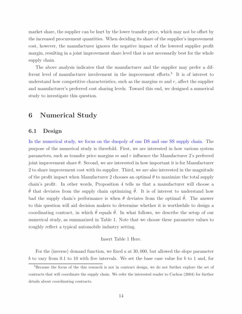
The above analysis indicates that the manufacturer and the supplier may prefer a dif-

ferent level of manufacturer involvement in the improvement efforts.5 It is of interest to

understand how competitive characteristics, such as the margins m and r, affect the supplier

and manufacturer’s preferred cost sharing levels. Toward this end, we designed a numerical

study to investigate this question.

6 Numerical Study

6.1 Design

In the numerical study, we focus on the duopoly of one DS and one SS supply chain. The

purpose of the numerical study is threefold. First, we are interested in how various system

parameters, such as transfer price margins m and r influence the Manufacturer 2’s preferred

joint improvement share θ. Second, we are interested in how important it is for Manufacturer

2 to share improvement cost with its supplier. Third, we are also interested in the magnitude

of the profit impact when Manufacturer 2 chooses an optimal θ to maximize the total supply

chain’s profit. In other words, Proposition 4 tells us that a manufacturer will choose a

θ that deviates from the supply chain optimizing θ. It is of interest to understand how

bad the supply chain’s performance is when θ deviates from the optimal θ. The answer

to this question will aid decision makers to determine whether it is worthwhile to design a

coordinating contract, in which θ equals θ. In what follows, we describe the setup of our

numerical study, as summarized in Table 1. Note that we choose these parameter values to

roughly reflect a typical automobile industry setting.

Insert Table 1 Here.

For the (inverse) demand function, we fixed a at 30, 000, but allowed the slope parameter

b to vary from 0.1 to 10 with five intervals. We set the base case value for b to 1 and, for

5Because the focus of the this research is not in contract design, we do not further explore the set of

contracts that will coordinate the supply chain. We refer the interested reader to Cachon (2004) for further

details about coordinating contracts.

14

symmetry, the range of values chosen for b was 0.1, 0.5, 1, 2, and 10. We note that, consistent

with the existing literature, we adopted the standard inverse demand function. Therefore,

with an inverse linear demand function, a higher b is associated with a lower price sensitivity

and vice versa.

In terms of the suppliers’ production cost, we assumed that both suppliers have identical

initial production cost c, which varies (in lock step) from 5, 000 to 25, 000 with a step size of

5, 000. Therefore we had in total 5 different values for the suppliers’ initial production cost.

The improvement parameter µ was fixed at 100.

For the transfer price policy parameters m and r, we varied both m and r from 0.1 to

0.5 with a step size of 0.1. This results in a factorial combination of 25 observations. We

then carried out a factorial combination of all the system parameters described above and

repeated the calculation for the optimal θ, θ, as well as performance metrics such as the

manufacturers’ and suppliers’ profits. Note that while the factorial combination described

above would in theory yield a total of 54 = 625 unique observations for each performance

metrics, we removed those corner solutions that did not satisfy the condition gc ≤ a ≤ 2gc,

leaving 236 observations, which ensures that the demand is nonnegative (see the footnote of

Corollary 3 where g is defined in Proposition 2).

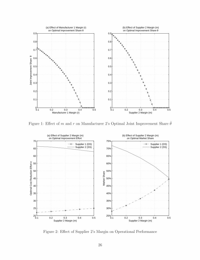
6.2 Optimal Joint Improvement Share θ

Proposition 2 characterizes the optimal θ that maximizes the manufacturer’s profit. Our

numerical study indicates that θ decreases in both m and r.

Insert Figure 1 Here.

Figure 1 indicates that the supplier margin m and the improvement cost sharing θ (by

Manufacturer 2) can be regarded as substitutes. When Manufacturer 2 sets a smaller (larger)

margin m for the supplier, then it is necessary and advantageous for it to share a larger

(smaller) fraction of its supplier’s improvement cost.

The fact that θ also decreases in r is interesting. Figure 1 indicates that when r increases

(i.e. Manufacturer 1 pays a lower transfer price to its supplier), Manufacturer 2 would share a

smaller fraction of its supplier’s improvement cost: by paying a lower transfer price p(1− r),

Manufacturer 1 becomes more competitive in the market (at the expense of Supplier 1).

Manufacturer 2 therefore sells less to the market and this dampens its incentive to help its

supplier on cost improvement.

Furthermore, our numerical results also show that θ on average decreases in the suppliers’

initial unit production cost c. This is somewhat counter-intuitive, because it suggests that

15

if the suppliers are not very efficient initially, then Manufacturer 2 will have less incentive

to help that supplier. Instead, Manufacturer 2 should be more willing to help a supplier

that are initially more efficient. Our interpretation is that the unit cost c influences a man-

ufacturer’s revenue potential: the higher the initial cost, the less revenue potential for both

manufacturers (or supply chains), and thus less incentive for improvement (improvement

expenses increase in the square of the cost reduction amount). This observation has an im-

portant practical implications for suppliers: it is better to improve production efficiencies to

a reasonable level first before expecting the manufacturer to help share the cost improvement

expense.

6.3 Effect of Supplier Margin (m) and Manufacturer Margin (r)

on System Performance

In our base model, we assume that Supplier 2’s margin m and Manufacturer 1’s margin r

are exogenous. In practice, however, both margins are subject to negotiations between the

manufacturer and the supplier. In what follows, we explore the effect of these margins on

the performance of the SS and DS supply chains using the above described numerical study.

First we focus on Supplier 2’s margin m. Figure 2 illustrates the effect of m on both

suppliers’ cost reduction effort, as well as the resulting market share of the two supply chains.


Notice that increasing Supplier 2’s margin m is not an attractive move for Manufacture 2:

It reduces the supplier’s cost reduction effort (Figure 2(a)) and it leads to a reduced market

share for the SS supply chain (Figure 2(b)). The intuition is that, with a higher profit

margin m, Manufacturer 2’s cost increases, hurting its market share. Therefore the optimal

improvement effort share θ decreases, causing Supplier 2 to lose incentive for cost reduction.

Figure 3 illustrates the profit impacts of increasing m.


Interestingly, even Supplier 2 could suffer from a very high margin m, as indicated in Figure

3(a). This is again due to a decreased market share, caused by a less competitive supply

chain as m increases. Overall, the SS supply chain suffers significantly from an increased

margin m (Figure 3(c)).

Therefore, we conclude that for the SS approach to be successful, it is imperative for

the manufacturer not to set a “fat” margin for the supplier. Instead, the manufacturer

16

should carefully balance the supplier’s margin m such that it is neither too small (such

that the supplier incurs losses) nor too high (such that the whole supply chain suffers).

This observation coincides with the examples discussed in the introduction, that a successful

implementation of SS approach requires the manufacturer understand the supplier’s cost

structurer precisely so as to set a reasonable margin for the supplier.

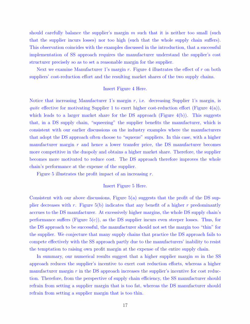
Next we examine Manufacturer 1’s margin r. Figure 4 illustrates the effect of r on both

suppliers’ cost-reduction effort and the resulting market shares of the two supply chains.


Notice that increasing Manufacturer 1’s margin r, i.e. decreasing Supplier 1’s margin, is

quite effective for motivating Supplier 1 to exert higher cost-reduction effort (Figure 4(a)),

which leads to a larger market share for the DS approach (Figure 4(b)). This suggests

that, in a DS supply chain, “squeezing” the supplier benefits the manufacturer, which is

consistent with our earlier discussions on the industry examples where the manufacturers

that adopt the DS approach often choose to “squeeze” suppliers. In this case, with a higher

manufacturer margin r and hence a lower transfer price, the DS manufacturer becomes

more competitive in the duopoly and obtains a higher market share. Therefore, the supplier

becomes more motivated to reduce cost. The DS approach therefore improves the whole

chain’s performance at the expense of the supplier.

Figure 5 illustrates the profit impact of an increasing r.


Consistent with our above discussions, Figure 5(a) suggests that the profit of the DS sup-

plier decreases with r. Figure 5(b) indicates that any benefit of a higher r predominantly

accrues to the DS manufacturer. At excessively higher margins, the whole DS supply chain’s

performance suffers (Figure 5(c)), as the DS supplier incurs even steeper losses. Thus, for

the DS approach to be successful, the manufacturer should not set the margin too “thin” for

the supplier. We conjecture that many supply chains that practice the DS approach fails to

compete effectively with the SS approach partly due to the manufacturers’ inability to resist

the temptation to raising own profit margin at the expense of the entire supply chain.

In summary, our numerical results suggest that a higher supplier margin m in the SS

approach reduces the supplier’s incentive to exert cost reduction efforts, whereas a higher

manufacturer margin r in the DS approach increases the supplier’s incentive for cost reduc-

tion. Therefore, from the perspective of supply chain efficiency, the SS manufacturer should

refrain from setting a supplier margin that is too fat, whereas the DS manufacturer should

refrain from setting a supplier margin that is too thin.

17

6.4 Effect of Price Sensitivity (b) on System Performance

One of the important market characteristics is the sensitivity of market price, that is, how

market price responds to total market supply. Recall that in our model we use the parameter

b in the demand function to capture the effect of price sensitivity on market supply. A higher

b value is associated with a higher price sensitivity. It is of interest, therefore, to understand

how market price sensitivity affects the DS and SS approaches’ performance.

First focus on the effect of price sensitivity b on the supply chain’s operational perfor-

mance. Figure 6 illustrates the effect of b on both suppliers’ cost reduction effort as well as

the resulting market share between the two supply chains.


Notice that, as the market price becomes more sensitive to the total supply (increasing

b), the supplier’s cost reduction efforts in both the DS and SS approaches decline rapidly

(Figure 6(a)), but the market share between the two approaches is much less sensitive to

changes in market price sensitivity (Figure 6(b)). Note that in Figure 6(b) the market share

for SS approach is much higher than that for DS approach; this is not due to inherent

superiority of the SS approach: it is merely a reflection of the base line values specified in

Table 1. Part of the intuition for the above observation is that, when price is very sensitive

to total market supply, the manufacturers have little incentive to compete on higher market

share (because the higher supply will leads to significantly lower market price) and therefore

they would not order as much from their respective suppliers. The suppliers then in turn

have little incentive to exert cost reduction effort, as doing so would not earn them higher

order quantities. From a managerial point of view, firms in industries that exhibit such high

price sensitivity often avoid destructive quantity competition, with a result that suppliers

often have little incentive to improve their production process. In such type of industry

environment, neither DS or SS approach can be effective to motivate the supplier to engage

in process improvement efforts.

Figure 7 directly illustrates the profit impacts of increasing the price sensitivity b.


Consistent with Figure 6, the above figure suggests that when the price sensitivity in-

creases, the supply chain performance for both DS and SS approach declines rapidly. Neither

DS nor SS approach seem to be effective in mitigating the negative impact of pronounced

market price sensitivity. In addition, there is little discernible difference between the DS and

SS approach in terms of the suppliers’ and manufacturers’ profits. Thus, the attractiveness

18

of the DS and SS approach is not significantly impacted by the market price sensitivity.

Instead, based on our earlier observations, whether the manufacturer prefers a DS or a SS

approach is primarily driven by how these two approaches are implemented through the

negotiations on supplier’s margin m (SS) and the manufacturer’s margin r (DS). In other

words, the success of the DS or SS approach is largely determined by whether they are

“correctly” implemented, as opposed to a particular market environment where the firms

reside.


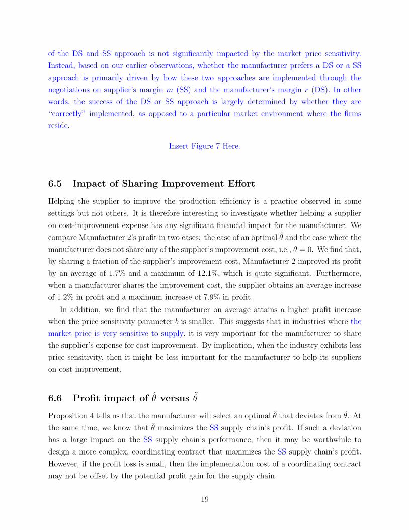
6.5 Impact of Sharing Improvement Effort

Helping the supplier to improve the production efficiency is a practice observed in some

settings but not others. It is therefore interesting to investigate whether helping a supplier

on cost-improvement expense has any significant financial impact for the manufacturer. We

compare Manufacturer 2’s profit in two cases: the case of an optimal θ and the case where the

manufacturer does not share any of the supplier’s improvement cost, i.e., θ = 0. We find that,

by sharing a fraction of the supplier’s improvement cost, Manufacturer 2 improved its profit

by an average of 1.7% and a maximum of 12.1%, which is quite significant. Furthermore,

when a manufacturer shares the improvement cost, the supplier obtains an average increase

of 1.2% in profit and a maximum increase of 7.9% in profit.

In addition, we find that the manufacturer on average attains a higher profit increase

when the price sensitivity parameter b is smaller. This suggests that in industries where the

market price is very sensitive to supply, it is very important for the manufacturer to share

the supplier’s expense for cost improvement. By implication, when the industry exhibits less

price sensitivity, then it might be less important for the manufacturer to help its suppliers

on cost improvement.

6.6 Profit impact of θ versus θ

Proposition 4 tells us that the manufacturer will select an optimal θ that deviates from θ. At

the same time, we know that θ maximizes the SS supply chain’s profit. If such a deviation

has a large impact on the SS supply chain’s performance, then it may be worthwhile to

design a more complex, coordinating contract that maximizes the SS supply chain’s profit.

However, if the profit loss is small, then the implementation cost of a coordinating contract

may not be offset by the potential profit gain for the supply chain.

19

We find that the SS supply chain’s total profit loss through the manufacturer’s selection

of θ is on average only 0.1%, with a maximum profit loss of 2.59%. We also find that the

supply chain’s profit loss is more pronounced when the demand slope parameter b is small

and when m and r are higher. Table 2 illustrates the profit loss when b = 0.1 and c = 15, 000.

Insert Table 2 Here.

We can see from Table 2 that the SS supply chain profit loss is higher when Manufacturer

2 sets a higher supplier margin m, or when Manufacturer 1 sets a higher manufacturer margin

r (i.e., Manufacturer 1 pays less to Supplier 1). This suggests that it might be worthwhile

to implement coordinating contracts when Supplier 2 enjoys a higher profit margin (m),

or when the competitor (Manufacturer 1) leverages its suppliers. In contrast, we find that

the SS supply chain profit loss diminishes when b becomes larger, suggesting that it is not

worthwhile to implement coordinating contracts in industries where price sensitivities are

low.

In summary, we find that helping suppliers to improve their production efficiencies is

quite important for the SS supply chain’s performance. In particular, it is more important for

Manufacturer 2 to help its supplier when the market exhibits high price sensitivities. Helping

suppliers by sharing their improvement costs is not entirely an altruistic action: it helps to

improve not only the supplier’s bottom line, but also the manufacturer’s profit. In addition,

it weakens the competition that uses a demand-side transfer price policy. On average, the

manufacturer enjoys a larger share of the benefits from a supplier’s cost improvement effort.

In general, the manufacturer’s optimal selection of θ does not seriously degrade the SS supply

chain’s performance, compared to the optimal sharing θ under a centralized supply chain.

Therefore, a simple linear transfer price contract is sufficient to guarantee that the whole SS

supply chain’s performance is close to optimality.

7 Conclusions

In this research, we contrast two often observed practices in target pricing; namely, the

supply-side approach and the demand-side approach. We derive a general oligopoly equi-

librium solution for the market price, the market share for each supply chain, and the

suppliers’ improvement efforts. Using a Cournot duopoly model, we fully characterize the

optimal policy when the two types of supply chains compete. We show that sharing the

cost-improvement expenses with its supplier proves to be a competitive advantage for the SS

supplier in the form of increased market share and higher profit. The competition of the two

20

supplier chains intensifies as a result of such sharing, leading to a decrease in the equilib-

rium market price and equilibrium transfer prices. In addition, the results indicate that the

optimal level of the manufacturer’s involvement in the supplier’s improvement effort is in-

fluenced by a number of system characteristics. [NEED TO UPDATE THE NUMERICAL

SUMMARY]Through our numerical study, we suggest that the manufacturer should help

the suppliers more in industries where the transfer price parameters m and r are lower, and

where the price sensitivities are higher. In addition, we point out that a manufacturer’s de-

viation from the supply chain’s optimal improvement cost sharing does not cause significant

profit loss.

There are a number of immediate extensions to this research. One potential extension

is to consider the scenario where the two manufacturers share a same supplier. In this

case, the benefit of one manufacturer’s joint improvement effort may spill over to the other

manufacturer because they share the same supplier.

In this paper, we examine a single-period oligopoly or duopoly model. In practice, cost

reduction occurs over time. One may also consider a multi-period model to study the time

effect of the target pricing policies. Intuitively, the time consideration will increase the

attractiveness of the supply-side policy as the manufacturer will be able to accumulate the

benefits of helping its suppliers. In each period, the starting cost c is a result of cost reduction

from previous time period, and thus retains the impact from the improvement effort of the

previous period. Therefore, the effect of high improvement effort (as well as the effort sharing

by the manufacturer) propagates through future time periods. As a result, we expect the

competition to be much more fierce and that both the suppliers and the manufacturers will

be more aggressive in choosing the improvement effort and the sharing of cost-improvement

expenses. Finally, one may study the incentive issues in setting the transfer price margins m

and r. We hope future studies by the authors and others will provide further insights into

the practice of target pricing.

Acknowledgement

The authors would like to thank Professor Christopher Tang, the seminar participants at the

Department of Supply Chain Management at Arizona State University and the attendees

at the INFORMS 2009 Western Regional Conference for their valuable comments on earlier

versions of this paper. The authors would also like to thank the Associate Editor and the

three anonymous referees for their helpful comments, which helped to improve the paper.

21

Appendix: Proofs

Proof of Proposition 1: First, we obtain e∗j =c(1+mj)Z−p

(1+mj)Z+µb(1−θj )/mj, j ∈ S where Z ≡

2 − 1/(

n + 1 − K +∑

k∈S rk

)

, and e∗k = rkpµb(1−θk)

, k ∈ S by optimizing the suppliers’ profits

in equation (3.5) and taking into consideration the facts that wk = p(1 − rk), k ∈ S and

wj = (c − ej)(1 + mj), j ∈ S. Then using p = (a +∑

ℓ wℓ)/(n + 1), and∑n

ℓ=1 wℓ =a(K−

∑

k∈Srk)+(n+1)

∑

j∈S(c−ej)(1+mj )

n+1−K+∑

k∈Srk

, and substituting e∗k and e∗j , we obtain a linear equation for

p and thus solve for the equilibrium market price p∗. Next, substitute p∗ into the expressions

for e∗j and e∗k to obtain the equilibrium investment effort. We omit the details here.

Proof of Corollary 1: With two symmetric DS supply chains, K = n = 2 and J = 0.

Thus,∑

k∈S rk = 2r and G = 0. The results follow immediately after substituting these into

Proposition 1.

Proof of Corollary 2: With two symmetric SS supply chains, J = n = 2 and K = 0. Thus,∑

k∈S rk = 0 and∑

j∈S Gj = 25/3+µb(1−θ)/[m(1+m)]

. The equilibrium price and investment effort

follow after substituting the above into Proposition 1 and applying algebraic transformation.

Proof of Corollary 3: With one DS and one SS supply chain, J = K = 1 and n = 2.

Thus,∑

k∈S rk = r and∑

j∈S Gj = 12−1/(r+2)+µb(1−θ)/[m(1+m)]

. The equilibrium price and

investment effort follow after substituting the above into Proposition 1 and applying algebraic

transformation.

Proof of Corollary 4: Assuming the condition a ≤ 2gc holds. Define

A =(1 − θ)µb(r + 2)[a + c(1 + m)] + (2r + 3)am(1 + m)

(1 − θ)µb(r + 2) + 2(1 + r)m(1 + m).

We can check that ∂A∂θ

= −µb(r+2)m(1+m)[2gc−a][(1−θ)µb(r+2)+2gm]2

≤ 0. Therefore statement 1) in Corollary

4 follows from Corollary 3 and the fact that p∗ = 1r+2

A. Statement 2) follows from the

expressions of q∗1 and q∗2 in Corollary 3 and the fact that ∂A∂θ

≤ 0 under the condition a ≤ 2gc.

Finally, statement 3) follows from Corollary 3 and the fact that ∂A∂θ

≤ 0.

Proof of Proposition 2: Statement 1) follows from the facts that ΠM∗1 = r2

b(r+2)2A2, and

A is decreasing in θ under the condition a ≤ 2gc.

To prove statement 2), we can show that∂ΠM∗

2

∂θ= mµ[2gc0−a]

(r+2)[(1−θ)µb(r+2)+2gm]3· [B(1 − θ) − D],

where B = µb(r + 2)[2g(a − gc) + 12(r + 2)m(2gc − a)] and D = (r + 2)m(2gc − a)[mg +

µb(r + 2)] − 2g2am. Assuming 0 ≤ θ ≤ 1 and under the conditiongc ≤ a ≤ 2gc, we havemµ[2gc0−a]

(r+2)[(1−θ)µb(r+2)+2gm]3≥ 0 and B ≥ 0. Therefore it follows that

∂ΠM∗2

∂θ≥ 0 if B(1−θ)−D ≥ 0,

or equivalently, θ ≤ 1 − D/B = θ; and∂ΠM∗

2

∂θ≤ 0 otherwise. This completes the proof.

Proof of Proposition 3: Statement 1) follows from the fact that∂ΠS∗

2

∂θ= 1

2µ(c− A−a

1+m)2 ≥ 0.

To show statement 2), as ΠS∗1 = 2µbr(1−r)+r2

2µb2(r+2)2A2 − cr

b(r+2)A (details omitted), we have

∂ΠS∗1

∂θ=

[2µbr(1−r)+r2

µb2(r+2)2A− cr

b(r+2)] · ∂A

∂θ. Therefore

∂ΠS∗1

∂θ≤ 0 iff 2µbr(1−r)+r2

µb2(r+2)2A− cr

b(r+2)≥ 0 (recall ∂A

∂θ≤ 0);

22

or equivalently, iff A ≥ cµb(r+2)2µb(1−r)+r

, which is equivalent to θ ≤ θ, where θ satisfies equation

(5.1). This completes the proof.

Proof of Proposition 4: Using the fact that ∂A∂θ

≤ 0 under the condition a ≤ 2gc, it

is easy to show that ΠS∗1 ≥ 0 is equivalent to θ ≤ ¯θ, where ¯θ satisfies A|θ=¯θ = 2cµb(r+2)

2µb(1−r)+r.

Comparing ¯θ with θ defined in (5.1), we have ¯θ < θ. Therefore ΠS∗1 ≥ 0 implies θ ≤ ¯θ < θ.

Statement 1) follows from Proposition 2 and Proposition 3. To show statement 2), we have∂Π∗

2

∂θ= ∂A

∂θ· 1(1+m)b(r+2)2 [(1−θ)µb(r+2)+2gm]

·[E−F (1−θ)], where E = µb(r+2)2m(2gc−a)−2g2am,

and F = µbm(r+2)2(2gc−a)+2µb(r+2)g(a−gc). As ∂A∂θ

≤ 0, 1(1+m)b(r+2)2 [(1−θ)µb(r+2)+2gm]

≥ 0

(assuming 0 ≤ θ ≤ 1), we know immediately that∂Π∗

2

∂θ≥ 0 if E−F (1−θ) ≤ 0, or equivalently,

if θ ≤ 1 − E/F = θ (notice F ≥ 0 under the condition gc ≤ a ≤ 2gc); and∂Π∗

2

∂θ< 0 if θ > θ.

Finally, statement 3) follows from the facts that E ≤ D and F ≥ B, where B and D are

defined in the proof of Proposition 2. This completes the proof.

References

[1] Agndal, H., Nilsson, U., 2008. Supply Chain Decision-Making Supported by an Open

Books Policy. International Journal of Production Economics 116, 154-167.

[2] Asanuma, B., 1985. The contractual framework for parts supply in the Japanese auto-

motive industry. Japanese Economic Studies, 13(14), 54-78.

[3] Ax, C., Greve, J., and Nilsson, U., 2008. The impact of competition and uncertainty on

the adoption of target costing. International Journal of Production Economics, 115 (1),

92-103.

[4] Babich, V., 2010. Independence of capacity ordering and financial subsidies to risky

suppliers. Manufacturing and Service Operations Management, 12(3), 583-607.

[5] Bernstein, F., Kok, A. G., 2009. Dynamic Cost Reduction Through Process Improve-

ment in Assembly Networks. Management Science, 55(4), 552-567.

[6] Cachon, G. P., 2004. The Allocation of Inventory Risk in a Supply Chain: Push, Pull,

and Advance-Purchase Discount Contracts. Management Science, 50(2), 222-238.

[7] Cooper, R., Yoshikawa, T., 1994. Inter-organizational cost management systems: The

case of the Tokyo - Yokohama - Kamakura supplier chain. International Journal of

Production Economics, 37 (1), 51-62.

23

[8] Cusumano, M. A., Takeishi, A., 1991. Supplier Relations and Management: A Survey of

Japanese, Japanese- Transplant, and U.S. Auto Plants. Strategic Management Journal,

12(8). 563-588.

[9] Ellram, L. M., 2006. The Implementation of Target Costing in the United States: Theory

Versus Practice. Journal of Supply Chain Management, 42(1), 13-26.

[10] Gilbert, S. M., Xia, Y., and Yu, G., 2006. Strategic outsourcing for competing OEMs

that face cost reduction opportunities. IIE Transactions, 38(11), 903 - 915.

[11] Gupta, S., Loulou, R., 1998. Process Innovation, Product Differentiation, and Channel

Structure: Strategic Incentives in a Duopoly. Marketing Science, 17(4), 301-316.

[12] Ha, A.Y., Tong, S., 2008. Contracting and Information Sharing Under Supply Chain

Competition. Management Science, 54(4), 701-715.

[13] Handfield, R. B., Krause, D. R., Scannell, T. V., and Monczka., R. M., 2004. Avoid the

pitfalls in supplier development. Sloan Management Review, 41(2), 37-49.

[14] Hartley, J. L., Choi, T. Y., 1996. Supplier development: Customers as a catalyst of

process change. Business Horizons, 39(4), 37-44.

[15] Helper, S. R., Sako, M., 1995. Supplier relations in Japan and the United States - are

they converging. Sloan Management Review, 36(3), 77-84.

[16] Li, L., 1985. Cournot Oligopoly with Information Sharing. The RAND Journal of Eco-

nomics, 16(4), 521-536.

[17] Li, L., 2002. Information Sharing in a Supply Chain with Horizontal Competition.

Management Science, 48(9), 1196-1212.

[18] Li, W., Humphreys, P.K., Yeung, A.C.L., and Cheng, T.C.E., 2007. The impact of spe-

cific supplier development efforts on buyer competitive advantage: an empirical model.

International Journal of Production Economics 106 (1), 230-247.

[19] Liker, J. K., Kamath, R. R., Nazli Wasti, S., and Nagamachi, M., 1996. Supplier in-

volvement in automotive component design: are there really large US Japan differences?

Research Policy, 25(1), 59-89.

[20] Liker, J., Choi, T. Y., 2004. Building Deep Supplier Relationships. Harvard Business

Review, 82(12), 104-113.

24

[21] Lovejoy, W.S., 2010. Bargaining Chains. Management Science 56, 2282-2301.

[22] Majumder, P., Srinivasan, A., 2008. Leadership and Competition in Network Supply

Chains. Management Science, 54(6), 1189-1204.

[23] Narayanan, V. G., Raman, A., and Singh, J., 2005. Agency Costs in a Supply Chain

with Demand Uncertainty and Price Competition. Management Science, 51(1), 120-132.

[24] Omar, O. E. 1997. Target pricing: a marketing management tool for pricing new cars.

Pricing Strategy and Practice, 5(2), 61-69.

[25] Wang, Y., Gilland, W., and Tomlin, B., 2010. Mitigating Supply Risk: Dual Sourcing

or Process Improvement? Manufacturing and Service Operations Management, 12(3),

489-510.

[26] Wu, O. Q., Chen, H., 2003. Chain-to-Chain Competition Under Demand Uncertainty,

Working Paper, University of British Columbia.

[27] Yao, D.-Q., Yue, X., and Liu, J., 2008. Vertical cost information sharing in a supply

chain with value-adding retailers. Omega, 36(5), 838-851.

[28] Zhang, H. 2002. Vertical information exchange in a supply chain with duopoly retailers.

Production and Operations Management 11(4), 531-546.

[29] Zhu, K., Zhang, R. Q., and Tsung, F., 2007. Pushing Quality Improvement Along

Supply Chains. Management Science, 53(3), 421-436.

Figures and Tables

25

0.1 0.2 0.3 0.4 0.50

0.1

0.2

0.3

0.4

0.5

0.6

0.7

0.8

0.9

Manufacturer 1 Margin (r)

Join

t Im

prov

emen

t Sha

re θ

(a) Effect of Manufacturer 1 Margin (r)on Optimal Improvement Share θ

0.1 0.2 0.3 0.4 0.50

0.1

0.2

0.3

0.4

0.5

0.6

0.7

0.8

0.9

Supplier 2 Margin (m)

(b) Effect of Supplier 2 Margin (m)on Optimal Improvement Share θ

Figure 1: Effect of m and r on Manufacturer 2’s Optimal Joint Improvement Share θ

0.1 0.2 0.3 0.4 0.520

25

30

35

40

45

50

55

60

65

70


Opt

imal

Cos

t Red

uctio

n E

ffort

e

(a) Effect of Supplier 2 Margin (m)on Optimal Improvement Effort

0.1 0.2 0.3 0.4 0.525%

30%

35%

40%

45%

50%

55%

60%

65%

70%

75%


Mar

ket S

hare

(b) Effect of Supplier 2 Margin (m)on Optimal Market Share

Supplier 1 (DS)Supplier 2 (SS)


Figure 2: Effect of Supplier 2’s Margin on Operational Performance

26

0.1 0.2 0.3 0.4 0.50

0.5

1.0

1.5

2.0

2.5

3.0

3.5


Sup

plie

r O

ptim

al P

rofit

(x1

07 )

(a) Effect of Supplier 2 Margin (m)on Supplier Optimal Profit

0.1 0.2 0.3 0.4 0.50

0.5

1.0

1.5

2.0

2.5

3.0

3.5


Man

ufac

ture

r O

ptim

al P

rofit

(x1

07 )

(b) Effect of Supplier 2 Margin (m)on Manufacturer Optimal Profit

0.1 0.2 0.3 0.4 0.51.0

1.5

2.0

2.5

3.0

3.5

4.0

4.5


Sup

ply

Cha

in O

ptim

al P

rofit

(x1

07 )

(c) Effect of Supplier 2 Margin (m)on Supply Chain Profit


Manufacturer 1 (DS)Manufacturer 2 (SS)

Supply Chain 1 (DS)Supply Chain 2 (SS)

Figure 3: Effect of Supplier 2’s Margin on Financial Performance

0.1 0.2 0.3 0.4 0.520

30

40

50

60

70

80

90

100


Opt

imal

Cos

t Red

uctio

n E

ffort

e

(a) Effect of Manufacturer 1 Margin (r)on Optimal Improvement Effort

0.1 0.2 0.3 0.4 0.510%

20%

30%

40%

50%

60%

70%

80%

90%


Mar

ket S

hare

(b) Effect of Manufacturer 1 Margin (r)on Optimal Market Share



Figure 4: Effect of Manufacturer 1’s Margin on Operational Performance

27

0.1 0.2 0.3 0.4 0.5−6.0

−5.0

−4.0

−3.0

−2.0

−1.0

0

1.0

2.0

3.0


Sup

plie

r O

ptim

al P

rofit

(x1

07 )

(a) Effect of Manufacturer 1 Margin (r)on Supplier Optimal Profit

0.1 0.2 0.3 0.4 0.50

1.0

2.0

3.0

4.0

5.0

6.0

7.0

8.0

9.0


Man

ufac

ture

r O

ptim

al P

rofit

(x1

07 )

(b) Effect of Manufacturer 1 Margin (r)on Manufacturer Optimal Profit

0.1 0.2 0.3 0.4 0.50

0.5

1.0

1.5

2.0

2.5

3.0

3.5

4.0

4.5


Sup

ply

Cha

in O

ptim

al P

rofit

(x1

07 )

(c) Effect of Manufacturer 1 Margin (r)on Supply Chain Profit




Figure 5: Effect of Manufacturer 1’s Margin on Financial Performance

0 2 4 6 8 100

100

200

300

400

500

600

700

800

Price Sensitivity (b)

Opt

imal

Cos

t Red

uctio

n E

ffort

e

(a) Effect of Price Sensitivity (b)on Optimal Improvement Effort

0 2 4 6 8 1020%

30%

40%

50%

60%

70%

80%


Mar

ket S

hare

(b) Effect of Price Sensitivity (b)on Optimal Market Share



Figure 6: Effect of Price Sensitivity on Operational Performance

28

0 5 100

0.5

1.0

1.5

2.0

2.5

3.0

3.5


Sup

plie

r O

ptim

al P

rofit

(x1

08 )

(a) Effect of Price Sensitivity (b)on Supplier Optimal Profit

0 5 100

0.5

1.0

1.5

2.0

2.5

3.0

3.5


Man

ufac

ture

r O

ptim

al P

rofit

(x1

08 )(b) Effect of Price Sensitivity (b)on Manufacturer Optimal Profit

0 5 100

0.5

1.0

1.5

2.0

2.5

3.0

3.5

4.0

4.5


Sup

ply

Cha

in O

ptim

al P

rofit

(x1

08 )

(c) Effect of Price Sensitivity (b)on Supply Chain Profit




Figure 7: Effect of Price Sensitivity on Financial Performance

29

Parameter a b c µ m r

Base Case 30,000 1 15,000 100 0.1 0.1

Range 30,000 (1) 0.1 ∼ 10 (5) 5,000 ∼ 25,000 (5) 100 (1) 0.1 ∼ 0.5 (5) 0.1 ∼ 0.5 (5)

Table 1: Numeric Study Setup (Number in bracket indicates number of scenarios)

r

m 0.1 0.2 0.3 0.4 0.5

0.1 0.00 0.01 0.02 0.04 0.10

0.2 0.03 0.07 0.16 0.35 0.87

0.3 0.12 0.28 0.65 1.68 1.79

0.4 0.37 0.89 2.34 1.81 -

0.5 0.98 2.59 2.02 - -

Table 2: Average SS supply chain profit loss in percentages (Dash ‘-’ indicates corner solu-

tions)

30

Target Pricing: Demand-Side Versus Supply-Side …ywang195/research/TargetPricing.pdf · Target...

Documents

Transcript of Target Pricing: Demand-Side Versus Supply-Side …ywang195/research/TargetPricing.pdf · Target...