talk - Reed College
61
The Modularity Theorem Jerry Shurman y 2 + xy + y = x 3 − x 2 − x − 14 −1, 0, −2, 4, 0, −2, 1, −4, 4, 6, 4, ...
Transcript of talk - Reed College

The Modularity Theorem
Jerry Shurman
y2 + xy+ y = x3 − x2 − x− 14
−1, 0, −2, 4, 0, −2, 1, −4, 4, 6, 4, . . .

This talk discusses a result called the Modu-
larity Theorem:
All rational elliptic curves
arise from modular forms.
Taniyama first suggested in the 1950’s that
a statement along these lines might be true,
and a precise conjecture was formulated by
Shimura. A 1967 paper of Weil provides strong
theoretical evidence for the conjecture. The
theorem was proved in the mid-1990’s for a
large class of elliptic curves by Wiles with a key
ingredient supplied by joint work with Taylor,
completing the proof of Fermat’s Last The-
orem after some 350 years. The Modularity
Theorem was proved completely around 2000
by Breuil, Conrad, Diamond, and Taylor.
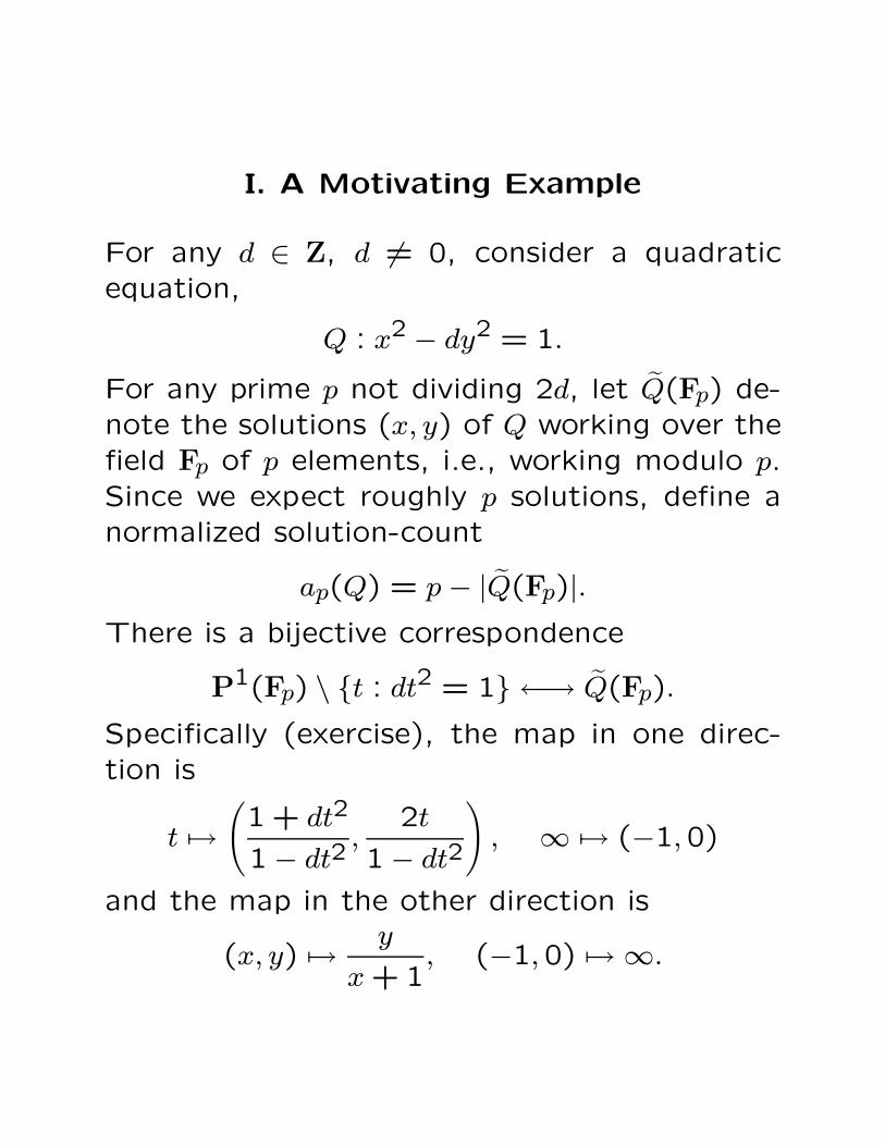
I. A Motivating Example
For any d ∈ Z, d 6= 0, consider a quadratic
equation,
Q : x2 − dy2 = 1.
For any prime p not dividing 2d, let Q(Fp) de-
note the solutions (x, y) of Q working over the
field Fp of p elements, i.e., working modulo p.
Since we expect roughly p solutions, define a
normalized solution-count
ap(Q) = p− |Q(Fp)|.
There is a bijective correspondence
P1(Fp) \ t : dt2 = 1 ←→ Q(Fp).
Specifically (exercise), the map in one direc-
tion is
t 7→
(1 + dt2
1− dt2,
2t
1− dt2
), ∞ 7→ (−1,0)
and the map in the other direction is
(x, y) 7→y
x+ 1, (−1,0) 7→ ∞.
But the set P1(Fp) \ t : dt2 = 1 contains
p− 1 elements or p+1 elements depending on
whether d is a square modulo p or not. This
shows that for p ∤ 2d,
the normalized solution-count ap(Q)
is the Legendre symbol (d/p).
One statement of the Quadratic Reciprocity
Theorem is that (d/p) for p ∤ 2d depends only
on the value of p modulo 4|d|.
This can be reinterpreted as a statement that
the sequence of prime index solution-counts,
a2(Q), a3(Q), a5(Q), . . . ,
arises as a system of eigenvalues.

To see this, let
N = 4|d|,
let G be the multiplicative group of integer
residue classes modulo N ,
G = (Z/NZ)∗,
and let VN be the vector space of complex-
valued functions on G,
VN = f : G −→ C.
For each prime p, define a linear operator Tp
on VN ,
Tp : VN −→ VN ,
given by
(Tpf)(n) =
f(pn) if p ∤ N,
0 if p | N.
Here the product pn ∈ G uses the reduction
of p modulo N .

Consider a vector f = fQ in VN associated to
the equation Q,
f : G −→ C
given by
f(n) = (d/n) for n ∈ G.
Here (d/n) is the Jacobi symbol, generalizing
the Legendre symbol (d/p). Because (d/n) de-
pends only on n (mod N) according to Quad-
ratic Reciprocity, this f defines values
an(f) = (d/n), n ∈ Z+, gcd(n,N) = 1.
Extend the definition to
an(f) = 0, n ∈ Z+, gcd(n,N) > 1.
Thus ap(f) = ap(Q) for all primes p, including
p | 2d.

Then the definition of Tp and then the defini-
tion of f give
(Tpf)(n) =
f(pn) if p ∤ N,
0 if p | N
=
(d/pn) = (d/p)(d/n) if p ∤ N,
0 if p | N
= ap(f)f(n) in all cases.
That is, f is an eigenvector for the operators Tpand the eigenvalues are ap(f),
Tpf = ap(f)f for all p.
Since ap(f) = ap(Q), this shows that the se-
quence ap(Q) is a system of eigenvalues as
claimed.
To reiterate, equation Q gave rise to an in-
teger N , a complex vector space VN endowed
with linear operators Tp, and an eigenvector
f whose Tp-eigenvalues ap(f) are the solution-
counts ap(E).

The Modularity Theorem can be viewed as giv-
ing an analogous result. For any
g2, g3 ∈ Z, g32 − 27g23 6= 0,
consider a cubic equation
E : y2 = 4x3 − g2x− g3.
Such equations define rational elliptic curves.
For each prime number p, define a normalized
solution-count ap(E) akin to ap(Q) from be-
fore,
ap(E) = p− |E(Fp)|.
One statement of Modularity is that again
the sequence of solution-counts ap(E)
arises as a system of eigenvalues.
But this time the eigenvalues arise from a mod-
ular form.

Recall that the first slide displayed an equation,
y2 + xy+ y = x3 − x2 − x− 14,
and some data,
−1, 0, −2, 4, 0, −2, 1, −4, 4, 6, 4, . . .
The equation, although in a slightly different
form from the cubic equation on the previ-
ous slide, describes a rational elliptic curve E.
The data are the first few associated solution-
counts ap(E).
The picture in the first slide, to be explained
soon, is the object from the modular forms
world that gives rise to the elliptic curve. It is
essentially the same elliptic curve, although in
a very different context.

A modular form is a particular kind of complex
valued function, to be described later in this
talk. The point for now is that by analogy with
the motivating example, associated to every
rational elliptic curve E there are
• a positive integer N (the conductor of E),
• a vector space VN of functions (certain mod-
ular forms, to be described),
• linear operators Tp on VN (the Hecke op-
erators),
• and a particular function f that is an eigen-
vector for all Tp.
The eigenvalues are the solution-counts ap(E).
We lead into Modularity and the definition of
a modular form with some geometry.

II. Modularity in Complex Analytic Terms
R: a group, a line.
Z: a lattice (discrete subgroup of full rank),
acts on R by the rule
n(x) = x+ n.
The quotient R/Z: a compact group, a topo-
logical circle.
Replacing Z by any lattice subgroup preserves
the quotient up to homothety. That is, there
is essentially only one geometric class of quo-
tients in this context.

C: a group, a plane.
Λ: a lattice, acts on C by the rule
λ(z) = z+ λ.
The quotient C/Λ: a compact group, a topo-
logical torus.
0
Ω1
Ω2

As Λ varies through the different lattice sub-
groups, the quotients form only one topolog-
ical class, but a punctured sphere’s worth of
geometrically distinct classes, represented by
the points of the Fundamental Domain:
D

H = τ ∈ C : Im(τ) > 0: a domain. It extends
to
H∗ = H∪Q ∪ ∞
with the horocircle topology for the new points:
The domain H∗ is not a group. But the mod-
ular group
SL2(Z) =
[a bc d
]: a, b, c, d ∈ Z, det = 1
(a discrete group) acts on it as fractional linear
transformations,
g(τ) =aτ + b
cτ + d, g =
[a bc d
]∈ SL2(Q), τ ∈ H∗.

The quotient SL2(Z)\H∗ is represented by the
points of D ∪ ∞ where D is again the Fun-
damental Domain. That is, D ∪ ∞ and its
SL2(Z)-translates tessellate H∗. The following
picture partially shows this for |Re(z)| ≤ 1/2,
and the tesselation extends Z-periodically to
all of H∗.

For each positive integer N , define a subgroup
of the modular group,
Γ0(N) =
[a bc d
]∈ SL2(Z) : c ≡ 0 (mod N)
.
Especially Γ0(1) = SL2(Z).
The quotient Γ0(N)\H∗: a compact Riemann
surface. The first slide represented this quo-
tient for N = 17:
Here there are two order-2 elliptic points, no
order-3 elliptic points, and two cusps, and the
Riemann surface is a torus.
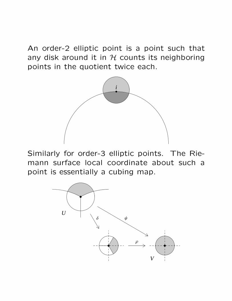
An order-2 elliptic point is a point such that
any disk around it in H counts its neighboring
points in the quotient twice each.
i
Similarly for order-3 elliptic points. The Rie-
mann surface local coordinate about such a
point is essentially a cubing map.
UΨ∆
Ρ
V

A cusp is a point where the quotient tapers to
a point at ∞ or at a rational number. Each
cusp has a width (the number of triangles that
meet there), and the Riemann surface local
coordinate about a cusp takes its width into
account.
h 1
U
∆ Ρ
Ψ
V

The number of elliptic points for Γ0(N) is
ε2(Γ0(N)) =
∏p|N(1 +
(−1p
)) if 4 ∤ N ,
0 if 4 | N ,
where (−1/p) is ±1 if p ≡ ±1 (mod 4) and is
0 if p = 2, and
ε3(Γ0(N)) =
∏p|N(1 +
(−3p
)) if 9 ∤ N ,
0 if 9 | N ,
where (−3/p) is ±1 if p ≡ ±1 (mod 3) and is
0 if p = 3.
The number of cusps of Γ0(N) is
ε∞(Γ0(N)) =∑
d|N
φ(gcd(d,N/d)).
See Helena Verrill’s website for a program that
draws pictures of these quotient Riemann sur-
faces and tracks associated arithmetic data,
e.g., elliptic points and cusps.

The Riemann surface Γ0(N)\H∗ is a sphere
with roughly N/12 handles. So the upper half
plane gives rise to all possible topological classes
of quotient, and in each topological class there
can be many geometric classses.
Thus the quotients Γ0(N)\H∗ are a rich source
of examples.
We now have enough geometry to state a ver-
sion of Modularity.

Let C/Λ be a complex torus. Consider two
complex constants associated to the lattice Λ,
g2 = 60∑
λ∈Λ
′λ−4, g3 = 140
∑
λ∈Λ
′λ−6.
(The primed sums mean to omit λ = 0.) Then
it is known that g32−27g23 6= 0. The j-invariantof C/Λ is
j = g32/(g32 − 27g23).
The complex analytic Modularity Theorem
is:
Let C/Λ be a complex torus with j ∈ Q. Then
for some N there is a nonconstant (and hence
surjective) holomorphic map of compact Rie-
mann surfaces
Γ0(N)\H∗ −→ C/Λ.
It is remarkable that so much number theory is
hidden here. Complex analysis is so rigid that
it is almost discrete.

III. Modular Forms and Arithmetic
Modularity
The usual measure on R satisfies d(x+n) = dx,
i.e., it is defined on the quotient R/Z,
d(n(x)) = dx.
Therefore, for a function f : R −→ R, the dif-
ferential f(x) dx is defined on the quotient if
and only if f is Z-periodic,
f(x+ n) = f(x), i.e., f(n(x)) = f(x).
For a meromorphic function f : C −→ C, the
differential f(z) dz similarly is defined on the
quotient C/Λ if and only if f is Λ-periodic,
f(z + λ) = f(z), i.e., f(λ(z)) = f(z).
The definition of modular forms arises from
analogous but more interesting considerations
on the upper half plane.

Recall that the 2-by-2 matrix group SL2(Z)
acts on the extended upper half plane H∗. For
any matrix γ ∈ SL2(Z) and any τ ∈ H, define
the factor of automorphy
j(γ, τ) = cτ + d where γ =
[a bc d
].
Note that j(γ, τ) has neither zeros nor poles.
The usual measure on H satisfies (exercise)
d(γ(τ)) = j(γ, τ)−2dτ.
So for a meromorphic function f : H −→ C, the
differential f(τ) dτ is defined on the quotient
Γ0(N)\H if and only if f satisfies the modu-
larity condition:
For all γ ∈ Γ0(N) and τ ∈ H,
f(γ(τ)) = j(γ, τ)2f(τ).

The general definition of a modular form is not
restricted to exponent 2, but it does impose
holomorphy conditions:
Let k be an integer and let N be a positive
integer. A modular form of weight k and
level N is a holomorphic function
f : H −→ C
such that for all γ ∈ Γ0(N) and all τ ∈ H,
f(γ(τ)) = j(γ, τ)kf(τ),
and such that f satisfies holomorphy condi-
tions at the cusps.
(The Modularity Theorem only needs weight
k = 2, the weight that we saw arise naturally
in the previous slide.)
Since the matrix γ =[1 10 1
]is in Γ0(N), and
since γ acts on H∗ as the translation τ 7→ τ+1,
and since j(γ, τ) = 1 for this γ and for all τ ,
every modular form is Z-periodic and therefore
has a Fourier expansion,
f(τ) =∞∑
n=0
an(f)qn, q = e2πiτ .
Modularity says that given a rational elliptic
curve E, some particular modular form f will
have prime index Fourier coefficients ap(f) that
match the mod p solution-counts ap(E) of E.
That is, the Fourier coefficients of modular
forms encode the modular arithmetic of ratio-
nal elliptic curves.

This is powerful because we know all about
modular forms. We can count them, and we
can write down the Fourier expansions of the
particular modular forms that give rise to el-
liptic curves. The actual data set has grown
tremendously over the past two decades thanks
to computational number theory. The infor-
mation can be seen at William Stein’s website.
Having described modular forms in general, we
need to do a bit more work to describe the
particular ones that figure in the Modularity
Theorem.

A cusp form is a modular form that “vanishes
at the cusps.” Since Im(τ) → +∞ if and only
if q → 0, vanishing at the cusp ∞ means that
the Fourier expansion of f has a0 = 0,
f(τ) =∞∑
n=1
an(f)qn, q = e2πiτ ,
Any other cusp can be moved to ∞ by an
SL2(Z) change of variables, and the cusp form
condition is that the Fourier expansion of the
correspondingly transformed f should also have
a0 = 0.

The simplest cusp form is the discriminant func-
tion ∆. For any τ ∈ H consider the lattice
Λ = τZ ⊕ Z. As before, we have lattice con-
stants g2 = g2(τ) and g3 = g3(τ). The dis-
criminant of τ is
∆(τ) = g2(τ)3 − 27g3(τ)
2.
(This is the denominator of the j-invariant from
earlier.) The discriminant is a cusp form of
weight 12 and level 1, i.e., for all τ ∈ H and
γ ∈ SL2(Z),
∆(γ(τ)) = j(γ, τ)12∆(τ).
For any positive N , the function ∆N(τ) =
∆(Nτ) is a cusp form of weight 12 and level N .

For any integer k and positive integer N , the
cusp forms of weight k and level N form a
finite-dimensional complex vector space
Sk(Γ0(N)).
(“S” stands for “spitz,” German for “cusp.”)
There are formulas for its dimension in terms
of the arithmetic data associated with the mod-
ular quotient Γ0(N)\H∗.
Especially for weight 2, let g be the genus
(number of handles) of Γ0(N)\H∗. Then
dim(S2(Γ0(N))) = g.

Although the Modularity Theorem only needs
k = 2, let k ≥ 4 be even, again let g be the
genus of Γ0(N)\H∗, and let ε2 be the number
of elliptic points with period 2, ε3 the num-
ber of elliptic points with period 3, and ε∞
the number of cusps. Then the dimension
dim(Sk(Γ0(N))) is
(k − 1)(g − 1) +
⌊k
4
⌋ε2 +
⌊k
3
⌋ε3 + (
k
2− 1)ε∞.
There are similar formulas for odd k, except
that the situation for k = 1 is trickier and not
completely understood. There are no nonzero
modular forms of negative weight and there
are no nonzero cusp forms of weight 0.

A canonical basis of Sk(Γ0(N))
The Hecke operators are linear operators on
the vector space Sk(Γ0(N)), defined as follows:
Let T1 = 1 (the identity operator).
For each prime p, define the operator Tp to
take each weight k cusp form at level N ,
f(τ) =∞∑
n=1
an(f)qn,
to (what can be shown to be) another weight
k cusp form at level N ,
(Tpf)(τ) =∞∑
n=1
an(Tpf)qn,
whose Fourier coefficients are derived from those
of f as follows:
an(Tpf) = anp(f) + 1N(p)pk−1an/p(f).

Here 1N is the trivial character modulo N ,
1N(p) =
1 if p ∤ N,
0 if p | N.
For prime powers, define inductively
Tpr = TpTpr−1 − pk−11N(p)Tpr−2, for r ≥ 2.
Finally extend the definition multiplicatively to
Tn for all n,
Tn =∏Tpeii
where n =∏peii ,
The Tp operator can be motivated in various
ways, but we don’t have time. We will mo-
tivate the prime power recurrence later in the
talk.

The Hecke operators are linear operators on
the finite-dimensional vector space Sk(Γ0(N))
over C. It can be shown that the Tn commute.
It also can be shown that the Tp for p ∤ N are
normal, i.e., they commute with their adjoints.
Consequently, by linear algebra, Sk(Γ0(N)) has
a basis of simultaneous eigenforms for all Tp,
p ∤ N .
Since we are obtaining these Hecke eigen-
forms by quoting an existence theorem, they
are not innately easy to write down. But they
are natural if the Hecke operators are naturally
motivated, which they are.

We don’t yet have Hecke eigenforms for all
the Tp, the problem being with the primes pdividing N . But this can be fixed.
Certain weight k, level N cusp forms actually
arise from lower levels M | N . These form a
subspace of Sk(Γ0(N)), the subspace of old-
forms. Also, the space Sk(Γ0(N)) has a natu-
ral inner product, the Petersson inner prod-
uct. The complementary space of the old-
forms with respect to the Petersson product is
the space of newforms.
Atkin and Lehner showed that the Tp-eigenforms
for all p ∤ N that are new at level N are in fact
Tp-eigenforms for all p.
Again, these are natural, they can be com-
puted by methods from computational num-
ber theory, and many of them are to be found
at William Stein’s website. Especially when
k = 2, these weight 2 new Hecke eigenforms
are the modular forms that appear in the Mod-
ularity Theorem.

Any Hecke eigenform can be normalized so
that its Fourier expansion is
f(τ) =∞∑
n=1
an(f)qn, a1(f) = 1,
and then the Fourier coefficients are the eigen-
values,
Tpf = ap(f)f.
It follows from the recursive definition of Tpr
that the prime power Fourier coefficients of
an eigenform at level N satisfy a recurrence
for r ≥ 2,
apr(f) = ap(f)apr−1(f)− pk−11N(p)apr−2(f).
This means that a certain Dirichlet series
takes the form of an Euler product. Let s
be a complex variable. Then formally
∞∑
n=1
an(f)n−s =
∏
p(1−ap(f)p
−s+1N(p)p1−2s)−1.
Both of these expressions are the L-function
of f , denoted L(f, s).

The prime power solution-counts apr(E) of a
rational elliptic curve with conductor N (these
are the normalized solution-counts working over
the field of pr elements) satisfy the analogous
recurrence for r ≥ 2,
apr(E) = ap(E)apr−1(E)− p1N(p)apr−2(E).
Comparing the exponents of p shows why in
particular we are interested in weight k = 2
newforms. Comparing the trivial characters
shows why we suspect that the newforms at
level N give rise to the rational elliptic curves
with conductor N .
The arithmetic Modularity Theorem is:
Let E be an elliptic curve over Q and let N
be its conductor. Then there is a new Hecke
eigenform f in S2(Γ0(N)) such that
ap(f) = ap(E) for all p.

A restatement of arithmetic Modularity is that
the L-function of some eigenform f is the L-
function of the elliptic curve E,
L(f, s) = L(E, s).
Here s is a complex variable and
L(E, s) =∏
p(1− ap(E)p−s + 1N(p)p1−2s)−1.
From the theory of modular forms, L(f, s) con-
verges on a right half plane of s-values, it has
an analytic continuation to all of the s-plane,
and the analytically continued function satis-
fies a functional equation. By Modularity, all
of this now applies to L(E, s).

This is important because the continued L(s, E)
is conjectured to contain sophisticated infor-
mation about the group structure of E. Specif-
ically, since E(Q) is a finitely generated Abelian
group it takes the form
E(Q) ∼= T ⊕ Zr,
where T is the torsion subgroup and r is the
rank. The rank is much harder to compute
than the torsion. However, the (weak) Birch
and Swinnerton-Dyer Conjecture says that
the rank of E(Q) is the order of vanishing of
L(s, E) at s = 1.
The Birch and Swinnerton-Dyer Conjecture would
give an algorithm for finding all rational points
on elliptic curves.

IV. From Complex Analysis to Rational
Algebraic Geometry
Recall that the Riemann surface Γ0(N)\H∗ is
topologically a g-handled sphere.
Its Jacobian J0(N) is defined complex analyt-
ically as path integration modulo integration
around loops (homology). This is an abelian
group. Geometrically it is a g-complex-dimen-
sional torus Cg/Λg. The Hecke operators take
homology to homology, so they act on the
quotient. Thus the Jacobian recovers a torus
structure from the Riemann surface, but the
dimension of the torus is the genus of Γ0(N)\H∗,
not generally 1.

The Modularity Theorem can be stated in terms
of Jacobians, thus incorporating group theory:
Let C/Λ be a complex torus with j ∈ Q. Then
for some N there is a nonconstant (and hence
surjective) holomorphic homomorphism of tori
J0(N) −→ E.

Next, the Jacobian J0(N) decomposes into a
product of abelian variety factors Af , where
each f is a weight 2 Hecke eigenform new at
level Mf and each Af is the quotient
Af = J0(Mf)/If(J0(Mf)).
Here If is the algebra generated over Z by the
Hecke operators Tp that take f to 0, and the
Hecke operators act on the Jacobian in a nat-
ural way. Thus the Hecke operators cut the
Jacobian into abelian varieties associated to
the eigenforms. The ring
Z[ap(f)]∼= Z[Tp]/If
naturally acts on Af . In particular, each ap(f)
acts on Af .
The abelian variety Af is again a complex torus
Cd/Λd and hence an abelian group. Its dimen-
sion d is the degree of the number field gener-
ated by the Fourier coefficients of f ,
dim(Af) = [Q(an(f)) : Q].

It is not immediately obvious that the field ex-
tension degree should be finite at all, but it
is. Also, the Fourier coefficients are algebraic
integers, not merely algebraic numbers.
Here we start to see connections between the
complex analysis and the arithmetic. Espe-
cially, the abelian variety Af is a 1-dimensional
torus C/Λ if and only if all the Fourier coeffi-
cients an(f) are rational integers.
The Modularity Theorem can be stated in terms
of abelian varieties:
Let C/Λ be a complex torus with j ∈ Q. Then
for some weight 2 new Hecke eigenform f ,
there is a nonconstant (and hence surjective)
holomorphic homomorphism of tori
Af −→ E.
This version associates a newform f to C/Λ.

So far our methods have been complex ana-
lytic, with arithmetic and number theory seem-
ing to play only an incidental role. But this is
misleading. All the complex analytic geometry
is in fact arithmetic and algebraic.
Returning to the real line: Let C be unit circle
in the plane R2,
C : x2 + y2 = 1.
The quotient R/Z maps to C via the trigono-
metric functions:
R/Z −→ C, x+ Z 7−→ (cos x, sinx).
This is a group isomorphism. (C has a group
structure as a subset of C∗.)

Returning to the complex plane: Again let Λ
be a lattice. Recall the two complex constants
g2 and g3 associated to the lattice Λ. Let E
be the elliptic curve with these constants as its
coefficients,
E : y2 = 4x3 − g2x− g3.
A change of variable makes g2 and g3 integral
if and only if the j-invariant is rational.
The quotient C/Λ maps to E via the Weier-
strass ℘-function and its derivative ℘′,
C/Λ −→ E, z + Λ 7−→ (℘(z), ℘′(z)).
This is a group isomorphism. (It is true but not
obvious that E has an abelian group structure
without reference to this map.)

By much more indirect methods:
All Riemann surfaces Γ0(N)\H∗, all Jacobians
J0(N), and all abelian varieties Af are described
by systems of polynomial equations over Z in
many variables.
In this context, the object associated to the
Riemann surface Γ0(N)\H∗ is denoted X0(N)
and called a modular curve. The object as-
sociated to the Jacobian J0(N) is an algebraic
construct called the Picard group of X0(N)
and denoted Pic(X0(N)), and the object as-
sociated with the abelian variety Af is again
called an abelian variety and denoted Af .
One way of describing the modular curve X0(N)
is by a single equation in two variables. This
is the modular equation.

For N = 2 the modular equation is
X0(2) : x3 + y3 − x2y2 + 1488xy(x+ y)
− 162000(x3 + y3) + 40773375xy
+ 8748000000(x+ y)
− 15764000000000 = 0.
The modular equation for N = 3 was found bySmith in 1878, for N = 4 by Berwick in 1916,
for N = 7 by Hermann in 1974. The smallest
N for which X0(N) is an elliptic curve is N =11. The modular equation for N = 11 took 20
hours to compute by MACYSMA on a VAX-
780 in 1984, required five pages to print, andhas coefficients up to 1060. It certainly doesn’t
look like the equation of an elliptic curve, and
yet it becomes such an equation under somevery complicated algebraic change of variable.
In general, the modular equation is hopelesslycomplicated, and its description of X0(N) can
include crossings and kinks. When described
by more equations in more variables, X0(N) issmooth. In any case, the modular equation for
its own sake is not the point.

Under the transition from complex analysis to
algebraic geometry over Q, the maps provided
by the earlier versions of Modularity become
maps defined by rational functions with coef-
ficients in Q,
X0(N) −→ E,
Pic(X0(N)) −→ E,
Af −→ E.
Applications of Modularity to number theory
typically rely on these algebraic versions of the
theorem. A striking example is the construc-
tion of rational points on elliptic curves, mean-
ing points whose coordinates are rational. The
key idea is that there is a natural construc-
tion of Heegner points on modular curves,
points with algebraic coordinates. Taking the
images of these points on elliptic curves under
the map X0(N) −→ E and then symmetrizing
gives points with rational coordinates.
V. From Algebraic Geometry to
Arithmetic
Let X0(N) be defined by the modulo p re-
ductions of the algebraic equations defining
X0(N).
It is Igusa’s Theorem that X0(N) defines a
smooth algebraic curve in characteristic p.
It is the Eichler–Shimura Relation that the
Hecke operator Tp on Pic(X0(N)) reduces mod-
ulo p to a map σ on Pic(X0(N)) that is well un-
derstood; specifically σ comes from the Frobe-
nius map x 7→ xp, a homomorphism in charac-
teristic p.

The route from algebraic Modularity to arith-
metic Modularity is, loosely, as follows: Given
a map α : X0(N) −→ E, we want the prime
index Fourier coefficients ap(f) for some f to
match the prime solution-counts ap(E) of E.
The ideas are:
• ap(f) acts on Af as Tp for each f , and a
sum of factors Af over all f is isogenous
to Pic(X0(N)).
• Tp on Pic(X0(N)) reduces modulo p to σ
on Pic(X0(N)).
• σ on Pic(X0(N)) commutes with α∗ to be-
come σ on Pic(E).
• σ on Pic(E) is ap(E).

Again, we are given α : X0(N) −→ E. The
relations in the previous slide can be expressed
in a commutative diagram incorporating nearly
everything mentioned in this talk:
⊕Af
∏ap(f)
//
⊕Af
Pic(X0(N))Tp
//
Pic(X0(N))α∗
//
Pic(E)
Pic(X0(N))σ
//
1
Pic(X0(N))α∗
// Pic(E)
1
Pic(X0(N))α∗
// Pic(E)ap(E)
// Pic(E).
This does not prove Modularity. It shows only
that the algebraic geometry version of Mod-
ularity implies the arithmetic version. Neither
version of Modularity here incorporates enough
algebraic structure to allow a proof.

VI. Galois Representations and Modularity
The version of the Modularity Theorem that
was finally proved is phrased in terms of the
additional structure of Galois representations:
All Galois representations
arising from rational elliptic curves
arise from modular forms.

Recall the ideas up to now:
Elliptic curves and modular curves are Riemann
surfaces and they are algebraic curves over C.
As a general principle, information about math-
ematical objects can be obtained from related
algebraic structures.
Elliptic curves already form Abelian groups.
Modular curves do not, but the complex vector
space S2(Γ0(N)) of weight 2 cusp forms at
level N has dimension g, the genus of X0(N),
the Hecke operators act on this vector space,
and integral homology is a lattice in the dual
space and is stable under the Hecke action.
This leads to the complex analytic Jacobian
J0(N), an Abelian group and a complex torus,
analogous to an elliptic curve but of dimension
g.

As number theorists we are interested in equa-
tions over number fields, in particular elliptic
curves over Q. The modular curves X0(N) are
defined over Q as well. As another general
principle, information about equations can be
obtained by reducing them modulo primes p.
Reducing the equations of elliptic curves and
modular curves gives similar relations for the
two kinds of curve: for an elliptic curve E
over Q,
ap(E) = σ
as an endomorphism of Pic(E),
while for the modular curve X0(N) the Eichler–
Shimura Relation is
Tp = σ
as an endomorphism of Pic(X0(N)).
These relations hold for all but finitely many p,
and each involves different geometric objects
as p varies.
The techniques that finally proved he Modu-
larity Theorem incorporate additional algebraic
structure into the picture. The idea is to lift
the two relations from characteristic p to char-
acteristic 0.
For any prime ℓ, the ℓ-power torsion groups of
an elliptic curve give rise to a vector space Vℓ(E)
over the ℓ-adic number field Qℓ. Similarly, the
ℓ-power torsion groups of the Picard group of a
modular curve give an ℓ-adic vector space Vℓ(X).
The vector spaces Vℓ(E) and Vℓ(X) are acted
on by the absolute Galois group of Q, the
group GQ of automorphisms of the algebraic
closure Q. This group subsumes the Galois
groups of all number fields, and it contains
absolute Frobenius elements Frobp for maxi-
mal ideals p of Z lying over rational primes p.
The vector spaces Vℓ(X) are also acted on by
the Hecke algebra.

The two relations in characteristic p lead to
the relations
Frob2p − ap(E)Frobp + p = 0
as an endomorphism of Vℓ(E)
and
Frob2p − TpFrobp + p = 0
as an endomorphism of Vℓ(X0(N)).
These hold for a dense set of elements Frobp
in GQ, but now each involves a single vector
space as Frobp varies. The second relation
connects the Hecke action and the Galois ac-
tion on the vector spaces associated to mod-
ular curves.
The vector spaces Vℓ are Galois representa-
tions of the group GQ. The Galois representa-
tion associated to a modular curve decomposes
into pieces associated to modular forms. The
Modularity Theorem in this context is that the
Galois representation associated to any elliptic
curve over Q arises from such a piece.

Let F be a Galois number field.
All but finitely many of its primes p define cor-
responding Frobenius elements Frobp of the
Galois group Gal(K/Q). Each Frobenius ele-
ment is related to the corresponding Frobenius
automorphism x 7→ xp in characteristic p.
The Tchebotarov Density Theorem states
that every element of the Galois group takes
the form Frobp for infinitely many primes p.
(This is a generalization of Dirichlet’s Theo-
rem on Arithmetic Progressions.)

Revisiting our motivating example:
Consider the Galois number field F = Q(d1/2).
Its Galois group is cyclic of order 2 (and there-
fore abelian),
Gal(F/Q) = 〈σ〉, σ : d1/2 7−→ −d1/2.
This group has a 1-dimensional representation
ρ : Gal(F/Q) −→ GL1(Z),
described by its action on Frobenius elements
for p ∤ 2d,
Frobp 7−→ (d/p).
Thus the values ρ(Frobp) are a system of eigen-
values ap(f), as before.

Even the simplest such example arising from
modular forms takes some work to describe.
Let d ∈ Z+ be cube-free. Consider the Ga-
lois number field F = Q(d1/3, ζ3). This is the
number field generated by the order-2 torsion
points of the elliptic curve y2 = x3− d. Its Ga-
lois group is nonabelian order 6 (the simplest
nonabelian group),
Gal(F/Q) = 〈σ, τ〉,
where
σ :
(d1/3 7→ ζ3d
1/3
ζ3 7→ ζ3
), τ :
(d1/3 7→ d1/3
ζ3 7→ ζ23
),
This group has a 2-dimensional representation
ρ : Gal(F/Q) −→ GL2(Z),
given by
σ 7→
[0 1−1 −1
], τ 7→
[0 11 0
].

The trace of ρ is a well defined function on
conjugacy classes
Frobp : p | p, p ∤ 3d,
i.e., it depends only on the underlying unram-
ified rational primes p. Specifically, trρ(Frobp)
is
2 if p ≡ 1 (mod 3), d is a cube mod p,
−1 if p ≡ 1 (mod 3), d not a cube mod p,
0 if p ≡ 2 (mod 3).
Similarly for the determinant of ρ,
det ρ(Frobp) =
1 if p ≡ 1 (mod 3),
−1 if p ≡ 2 (mod 3).

The representation ρ arises from modular forms
as follows. Using the Cubic Reciprocity The-
orem and Poisson summation, Hecke (1927)
constructed a class of functions including a
particular theta function,
θχ(τ) =∞∑
n=1
an(θχ)qn ∈ S1(27d
2, ψ),
where ψ is the quadratic character with con-
ductor 3, such that for all p ∤ 3d,
trρ(Frobp) = ap(θχ),
det ρ(Frobp) = ψ(p).
So the Galois group representation ρ, as de-
scribed by its trace and determinant on Frobe-
nius elements, arises from the modular form θχ.
This modular form is a normalized eigenform
and a cusp form. The Modularity Theorem
states that 2-dimensional representations of Ga-
lois groups arise from such modular forms in
great generality.

VII. That Application
The relation of all this to Fermat’s Last The-
orem is that nontrivial solution of the Fermat
equation
aℓ + bℓ = cℓ, ℓ prime
would give rise to the corresponding Frey curve
E : y2 = x(x− aℓ)(x+ bℓ).
The Fermat equation reduces to the case
gcd(a, b, c) = 1, a ≡ −1 (mod 4), b even.
The number field generated by the ℓ-torsion
points of E is unramified away from 2 and ℓ,
and even the ramification there is very small.
Consequently, the Frey curve must must arise
from a weight 2 modular form at level 2. But
S2(Γ0(2)) = 0, and so there is no such mod-
ular form. By contraposition, Fermat’s theo-
rem follows.