Talbot 2016 - Northwestern Universityebelmont/talbot... · 2018-08-23 · Disclaimer These are...
76
Talbot 2016: Equivariant homotopy theory and the Kervaire invariant one problem (notes from talks given at the workshop) Notes taken by Eva Belmont Last updated: May 16, 2016 1
Transcript of Talbot 2016 - Northwestern Universityebelmont/talbot... · 2018-08-23 · Disclaimer These are...

Talbot 2016:Equivariant homotopy theory
and the Kervaire invariant one problem
(notes from talks given at the workshop)
Notes taken by Eva Belmont
Last updated: May 16, 2016
1

Disclaimer
These are notes I took during the 2016 Talbot Workshop. I, not the speakers, bear respon-sibility for mistakes. If you do find any errors, please report them to:
Eva Belmontekbelmont at gmail.com
Thanks to all the participants who submitted corrections and revisions.
2

Contents
1. Introduction (Doug Ravenel) 5
2. Sketch of the proof (Mike Hill) 5
Main steps in proof; crash course in equivariant homotopy; ΩO; slice filtration and
slice theorem
3. The odd-primary Arf invariant (Foling Zou) 8
Ravenel’s proof that the p > 3 analogue of h2j dies
4. Review of category theory (Yexin Qu) 12
Kan extensions, ends and coends, monoidal categories, enriched functors, Day
convolution
5. Equivariant homotopy theory I (J.D. Quigley) 15
G-CW complexes, representation spheres, examples
6. Introduction to equivariant homotopy theory II (Fei Xie) 17
Orthogonal G-spectra, isotropy separation sequence, geometric fixed points, Mackey
functors
7. Model categories I (Ugur Yigit) 20
Model category axioms, cofibrantly generated model category
8. Model categories II (Alex Yarosh) 24
Kan recognition theorem and Kan transfer theorem, Bousfield localization, strict and
stable model structures on simplicial spectra
9. The Mandell-May definition of G-spectra (Renee Hoekzema) 26
Orthogonal spectra; orthogonal G-spectra; tautological presentation; smash product
of spectra
10. The homotopy category of SG (Allen Yuan) 30
Showing that ∨,∧,∏ are homotopical; −∧ SV and −∧ S−V are inverse equivalences
11. The positive complete model structure and why we need it (Hood Chatham) 36
3

(what the title says)
12. The norm construction and geometric fixed points (Benjamin Bohme) 42
Abstract framework behind NGH as an indexed smash product; Quillen adjunction
between NGH and ResGH ; geometric fixed points and its good properties; EF ; monoidal fixed
points functor ΦGM ; relationship between NG
H and ΦGH
13. The slice filtration and slice spectral sequence (Koen van Woerden) 45
Slice cells; slice tower; convergence; P−1−1 and P 0
0 ; relationship to Postnikov filtration;
n-null, n-positive; multiplicative properties
14. Dugger’s computation for real K-theory (Agnes Beaudry) 49
Atiyah real vector bundles; KO and KR; computation of πC2∗ KR
15. MU ((G)) and its slice differentials (Eva Belmont) 56
Definitions of MUR and MU ((G)); elements in the E2 page of the slice spectral
sequence for MU ((G)); slice theorem preview; computation of a differential in the spectral
sequence
16. The reduction, gap, and slice theorems (Akhil Mathew) 61
Proof of the gap theorem including cell lemma; building PnMU ((G)); statement of
reduction and slice theorems
17. The periodicity theorem and the homotopy fixed point theorem (Mingcong Zeng) 65
(what the title says. . . )
18. The detection theorem (Zhouli Xu) 68
Detection theorem from the algebraic detection theorem; review of formal group laws;
group actions on formal group laws; Ext∗∗MU∗MU (MU∗,MU∗)→ H∗(G,R∗) for the right R
19. Further directions (Doug Ravenel) 72
p = 3 case; θ6; EHP sequence; dream
4

Equivariant homotopy theory Talk 2
Notation
πuX nonequivariant (underlying) homotopy of X
i∗HX restriction of the G-spectrum X to an H-spectrum
S category of (orthogonal) spectra (9.2)
SG category of (orthogonal) G-spectra (9.7)
J indexing category for orthogonal spectra (9.3)
JG Mandell-May indexing category for orthogonal G-spectra (9.6)
MUR see beginning of Talk 15
MU ((G)) see beginning of Talk 15
T G objects are based G-spaces, morphisms are equivariant continuous maps
TG objects are based G-spaces, morphisms are all continuous maps
Talk 1: Introduction (Doug Ravenel)
See Doug Ravenel’s slides.
Talk 2: Sketch of the proof (Mike Hill)
Theorem 2.1. There are manifolds of Kervaire invariant one only in dimensions 2, 6, 14, 30, 62and possibly 126.
The first step was to take Browder’s work with the Adams spectral sequence (ASS) Ext∗∗A (F2,F2) =⇒πs∗; Browder’s theorem says that h2
j ∈ Ext2,2j+1is a permanent cycle iff there is a manifold of
Kervaire invariant 2j − 2. (Really it’s a coset of manifolds – it’s modulo Adams filtration.)
There is a map from the Adams-Novikov spectral sequence Ext2,2j+1
MU∗MU (MU∗,MU∗) to the
ASS sending β2j+1/2j−1 + noise 7→ h2j . This is detected in Adams filtration 0, 1, or 2. But
filtration 0 just has rational information which is known, and filtration 1 is just the imageof J , which is also known. The only possibility is filtration 2. The question is whether thereare any β2j+1/2j−1 that are permanent cycles.
MU∗MU is recording all possible isomorphisms between formal groups. Given a chosenformal group law, together with a collection of automorphisms, then we get a map from Extover all possible automorphisms to a smaller Ext, which records just the formal groups thatwe care about, in our case H2(C8;π2j+1R). This is the E2 term for the homotopy fixed pointspectral sequence for π∗(R
hC8). This style of argument (except for the ASS part) is whatDoug did for an odd prime. You have classes β2j+1/2j−1 to the homotopy fixed point spectralsequence that takes the kernel to 0. There’s a refinement due to Hopkins and Miller, namelythe Lubin-Tate spectrum E4; Hopkins-Miller says that C8 acts on this, and H2(C8;π2j+1R)is the corresponding ASS E2 page. The problem is that it’s too big.
5

Equivariant homotopy theory Talk 2
That was too hard, so we made it harder by adding more structure; there are fewer thingsthat can go wrong if there’s more structure.
Instead, we compute homotopy groups of actual fixed points. The strategy is four-fold:
(1) (Detection theorem) We produce a C8-spectrum ΩO such that that Kervaire classes are
detected in π∗ΩhC8O . (So I can use Ω in place of R, and everything I said goes through.)
(2) (Gap theorem) π−2ΩC8O = 0
(3) (Periodicity theorem) πk+256ΩhC8O∼= πkΩ
hC8O
(4) (Homotopy fixed point theorem) ΩC8O'→ ΩhC8
O
The first theorem is classical – it’s similar to what Doug did in the odd primary case. Theother theorems come from the use of a new tool, the slice spectral sequence.
2.1. Extremely crash course in equivariant homotopy. We’ll see some models asthe week progresses, but I need the following thing. We want to have a notion of G-spectra(we’ll stick with finite G) with the following properties:
(1) It should be like the usual category of spectra (cofiber sequences are fiber sequences, etc.)
(2) If X,Y are finite G-CW complexes1 then
[Σ∞+ X,Σ∞+ Y ] ∼= lim−→
V a f.d.rep of G
[ΣV+X,Σ
Y+Y ]G
Declare these to be the hom objects. Everything in sight is an abelian group, cofibersequences are fiber sequences, finite wedges are finite products, etc. You have to closethings up under various limit and colimit constructions. The downside is that Alexanderduality doesn’t work like it does in the classical case, where you use that to get from theSpanier Whitehead category to spectra.
(3) Finite G-sets are self-dual:
[G/H+ ∧ E,F ] ∼= [E,G/H+ ∧ F ].
(4) The category is a closed symmetric monoidal category under − ∧ −. Closed meanssmashing with a fixed spectrum has a right adjoint (internal hom).
(5) Representation spheres are invertible: SV ∧ S−V ' S0. This is what Doug talked aboutwhen he said we had an RO(G)-grading. Invertible objects are now exactly the repre-sentation spheres.
(6) If H ⊂ G have a restriction i∗H : SG → SH and this has both adjoints, induction G+∧H−and coinduction FH(G+,−), and we want G+ ∧H X
∼→ FH(G+, X).
3, 5, and 6 are equivalent. In spaces, I have the map in 6 but it’s almost never an equivalence:on the right, the group acts by moving the factors around and the fixed points are the diagonal;on the left, there are no fixed points (it’s just a bunch of copies of X stacked). This is sayingsomething essential about stability.
Write this as∨G/H X
∼→∏G/H X. So in the stable world, finite wedges are finite products.
1it has cells of the form G/H ×Dn, where the group acts in the obvious way on the left and trivially on thedisc
6

Equivariant homotopy theory Talk 2
Here are some consequences. [E,F ] extends to a pair of functors (SetG)op : T 7→ [T+ ∧E,F ]and SetG : T 7→ [E, T+ ∧ F ]. Self-duality says that the values are naturally isomorphic. Sothese agree on objects but I have really different maps: the first are called restriction maps,and the second are called transfers.
Why restriction? Look at G/H → ∗ and E = S0. Associated to this I have a map [∗+ ∧S0, F ]→ [G/H+∧S0, F ]; these are equivariant maps from S0 → F , and S0 has no action. Sothe LHS is [S0, FG] (where FG means G-fixed points) and the RHS is [G+ ∧H S0, F ]. Usingthe adjoint, this is [S0, FH ]. So this map is [S0, FG] → [S0, FH ]: G-fixed points restrict toH-fixed points.
We have a second kind of homotopy group: for V ∈ RO(G), πV (E) = [SV , E]. (Note thatI’m only writing [−,−]G in the unstable case.) We have a multiplicative version of induction– the norm. For intuition’s sake, if the transfer is summing all the cosets, think of the normas multiplying all the cosets, and it’s a universal Hom for a multiplication (just like tensorproduct of a module is universal Hom for multiplying). The norm is a functor NG
H : SG → SGsatisfying
• NGHS
V ' SIndGH V for V ∈ RO(H)
• NGH commutes with sifted colimits. If I write something as the geometric realization of a
simplicial thing, I can just take the norm of the simplicial levels.
• NGH is a strong symmetric monoidal functor for the smash product: NG
H (E∧F ) = NGH (E)∧
NGH (F ). In particular, it’s lax monoidal – it takes commutative monoids under ∧ to
commutative monoids under ∧.
• So it’s the left adjoint to the forgetful functor from CommG → CommH (where CommG
means G-equivariant commutative monoids).
• ΦNGH ' ΦHE (here I really mean just a homotopical statement, whereas the previous ∼= is
point-set level). “The failure of the norm to be additive is exactly what Φ is destroying.”
2.2. What is ΩO? First take NC8C2MUR; the underlying spectrum is MU∧4, and the
underlying C2-spectrum is MU∧4R . We know that π8
∗(MC8C2MUR) ∼= π∗(MU∧4) ∼= L⊗4 (where
L is the Lazard ring). (But note that the last ∼= is not a canonical isomorphism.) The actionof C8 permutes the factors, and when you come back around you use complex conjugation,which corresponds to the [−1] series. That is, (a, b, c, d) 7→ (d, a, b, c).
We can write π∗(MU∧4) as Z[r1, γr1, γ2r1, γ
3r1, r2, γr2, . . . ] where |ri| = 2i and γ is a gener-ator of C8, and the C8-action is:
γ · (γjrk) =
γj+1rk j + 1 ≤ 3
(−1)krk j + 1 = 4
Given a monomial p ∈ (π∗MU4) ⊗ Z/2, let Hp = Stab(p) and ‖p‖ = |p||Hp| · ρHp . Mod 2, the
(−1) above goes away, and C2 fixes every generator, so C2 ⊂ Hp ⊂ C8.
Let ΩO = D−1NC8C2MUR. I’m not going to say what D is, because it’s what works. This
element is in πC819ρ8
NC8C2MUR. Regular representations are a nice family: they always restrict
and induce to other regular representations.
7

Equivariant homotopy theory Talk 3
Slice filtration. The spaces in MU are Thom spaces of Grassmannians BU(n). GLn(C)have a Schubert decomposition describing its cell structure. If I evaluate on C, I have cellsthat look like Ck, and this is true equivariantly. In particular, C2 acts on C by complexconjugation, and turns Ck into kρ2. So we have a filtration of MU(n) with filtration quotientsSkρ2 .
The norm commutes with sifted colimits; a cell structure is a sort of sifted colimit. SoNC8C2MU has a cell structure with “cells” C8+ ∧H D(kρH) for C2 ⊂ H ⊂ C8. I attach disks
along the boundary spheres; this is the slice filtration.
The slice filtration is the filtration induced by the collections
G+ ∧H SkρH−ε : k · |H| − ε ≥ n, ε = 0, 1.So you should think of the −1 as coming from attaching maps of Schubert cells. After thefact, it turned out that you didn’t need to do that. (If you ignore the equivariance, this isthe Postnikov filtration.)
The big theorem that makes everything else run is the slice theorem.
Theorem 2.2 (Slice theorem). The slice associated graded of NC8C2MUR (Σkρ8NC8
C2MUR) is
of the form ( ∨p monomial in
(π∗(MU∧4)⊗Z/2)
C8+ ∧Hp S‖p‖)∧HZ
Here HZ is the spectrum computing Bredon homology with coefficients in Z.
Geometric fixed points are so named because it corresponds with your geometric intuition forfixed points: it commutes with Thom spectra and suspensions. In particular, ΦC2BU(n) =BO(n). Leveraging this allows you to get all the differentials you need in the slice spectralsequence.
Fact: (HZ)(V ) = ZSV /Z · ∗. HZ is the 0th Postnikov section of MU .
Talk 3: The odd-primary Arf invariant (Foling Zou)
(Note: this talk is about Ravenel’s paper “The non-existence of odd primary Arf invariantelements in stable homotopy”, 1978.) The methods used to prove the non-survival of the Arfinvariant element for p > 3 is the idea behind the HHR detection theorem.
Recall the Adams spectral sequence Es,t2 = Exts,tAp(Fp,Fp) =⇒ πt−s(S0)⊗ Zp. (We write Ap
for the mod-p Steenrod algebra.) The Er page has differentials dr : Es,t → Es+r,t+r−1. Thediagram is bigraded (s, t− s) such that differential dr maps 1 leftwards and r upwards. s iscalled the filtration and r − s is called the stem.
In the 0-line (i.e. s = 0), there is just one element (at (0, 0)). For p = 2, the 1-line consists
of elements hi ∈ Ext1,2i
A2which correspond to the Steenrod operations Sq2i . The survival of
hi is equivalent to the existence of Hopf invariant 1 map in suitable degree. By a theorem of
8

Equivariant homotopy theory Talk 3
Adams that, for i ≥ 4, hi does not survive, and the differential that kills it is d2hi = h0h2i−1.
For p > 2, the 1-line consists of elements hi ∈ Ext1,qpi
Apfor q = 2(p − 1), which correspond
to the odd Steenrod operations P pi, and a0 ∈ Ext1,1
Ap, which corresponds to the Bockstein β.
For i ≥ 1, there is a differential d2hi = a0bi−1. You should think of the bi’s as analogous tothe h2
i−1 elements for p = 2.
In the 2-line, there are Arf invariant elements. In the p = 2 case, they are h2i . The name
comes from a theorem of Browder which says that h2i is a permanent cycle iff there is a
manifold (of suitable dimension) of Arf invariant 1. It is known that for i ≤ 5 they survive.The main HHR theorem is that for i ≥ 7 they don’t. And i = 6 is still open.
In the p > 2 case, let bi = −〈hi, . . . , hi〉 be the p-fold Massey product. This is just h2i for
p = 2.
Aside: The analogy between h2i and bi can also be seen in the following example. For p > 2,
H∗(Z/p;Z/p) = E[h]⊗P [b] where b = 〈h, . . . , h〉 and for p = 2, H∗(Z/2;Z/2) = P [h] (there’sno b here because “b” = h2).
bi corresponds the an Adem relation involving P (p−1)piP pi. b0 survives. The main result of
the paper is to prove that for p > 3, bi does not survive for i ≥ 1. For p = 3, one step of theproof doesn’t work, and it turns out that b1 does not survive, b2 survives, and it is open fori ≥ 3.
The first result in this direction is by Toda.
Theorem 3.1 (Toda). d2p−1b1 = h0bp0
This introduces the hope of nontrivial differentials d2p−1bi = h0bpi−1, but this hope was
discouraged by a calculation of May, who showed that for p = 3, h0b31 = 0.
The paper uses the ANSS instead of the ASS to get over this obstacle.
Recall the Brown-Peterson spectrum BP , which has coefficient ring BP∗ = Z(p)[v1, v2, . . . ]
with |vi| = 2(pi − 1), and BP∗BP = BP∗[t1, t2, . . . ] with |ti| = 2(pi − 1). This gives theAdams-Novikov spectral sequence
Exts,tBP∗BP (BP∗, BP∗) =⇒ πt−s(S0)⊗ Zp.
There is a spectrum map BP → HZ/p which gives a map from the ANSS to the ASS; ithappens that they converge to the same thing outside the 0-stem.
We want to show:
Theorem 3.2. If p > 3 and i ≥ 1, then bi does not survive the ASS.
and we break it into two steps.
9

Equivariant homotopy theory Talk 3
Step 1. Find a representative of the preimage of this bi in the ANSS. In the cobar construc-tion,
bi = −∑
0<j<pi+1
1
p
(pi+1
j
)[tj1|tp
i−j1 ] and h0 = −[t1].
Theorem 3.3. For p ≥ 3, d2p−1bi+1 6= 0 for all i ≥ 0 in the ANSS.
Step 1.1 By induction on Toda’s theorem, and the relation hi+1bp1 = hi+2b
p0 obtained by
applying Steenrod operation to another relation from cobar construction, one can show that
d2p−1bi+1 = h0bpi mod ker bai0 , where ai = p(pi−1)
p−1 .
Step 1.2. The nontrivial step is to show that h0bi00 · · · · · bikk 6= 0, bi00 · · · · · bikk 6= 0 in
ExtBP∗BP (BP∗, BP∗), so that the differential is indeed nontrivial.
The idea is that, for n = p− 1, the construction of a map:
ExtBP∗BP (BP∗, BP∗) // ExtHomc(Fpn [Sn],Fpn )(Fpn ,Fpn) //
∼=
ExtHom(Fpn [Z/p],Fpn )(Fpn ,Fpn)
∼=
ExtFpn [Sn](Fpn ,Fpn) // ExtFpn [Z/p](Fpn ,Fpn)
H∗c (Sn;Fpn) // H∗(Z/p;Fpn) = E[h]⊗ P [b]
(3.1)
takes h0 7→ −ch and bi 7→ −cpi+1b for a nontrivial constant c. Here Sn is the Morava stabilizer
group that will be explained later, and when n = p− 1 it has a subgroup of order p.
Step 2. For p > 3, bi+1 in the ASS does not survive. (Theorem 3.3)
Since there is a map of spectral sequences ANSS to ASS, if x = bi+1 survives in ASS, thenthere is some x in the ANSS which survives to the same thing. It has to have filtration s ≤ 2,but either 0 or 1 is not possible because of sparseness in the E2 page of ANSS and stemcalculations. So x has to have filtration 2, and be a preimage of x under the map.
Miller-Ravenel-Wilson showed that
Lemma 3.4. Ext2,qpi+2
BP∗BP(BP∗, BP∗) is generated by βai,j/pi+3−2j for j = 1, 2, . . . ,
⌊i+3
2
⌋, where
ai,j = (pi+2 + pi+3−2j)/(p + 1). If j = 1, then βpi+1/pi+1 = bi+1. The map of SS takes thej > 1 elements to 0.
Then x looks like bi+1 + y where y is the “noise” generated by the beta elements with indexj > 1. Our goal is to filter these noise out by a detection map.
Lemma 3.5. Under the natural map
ExtBP∗BP (BP∗, BP∗)→ ExtBP∗BP (BP∗, BP∗/I3)
10
Equivariant homotopy theory Talk 3
where I3 = (p, v1, v2), βai,j/pi+3−2j (j > 1) maps to 0.
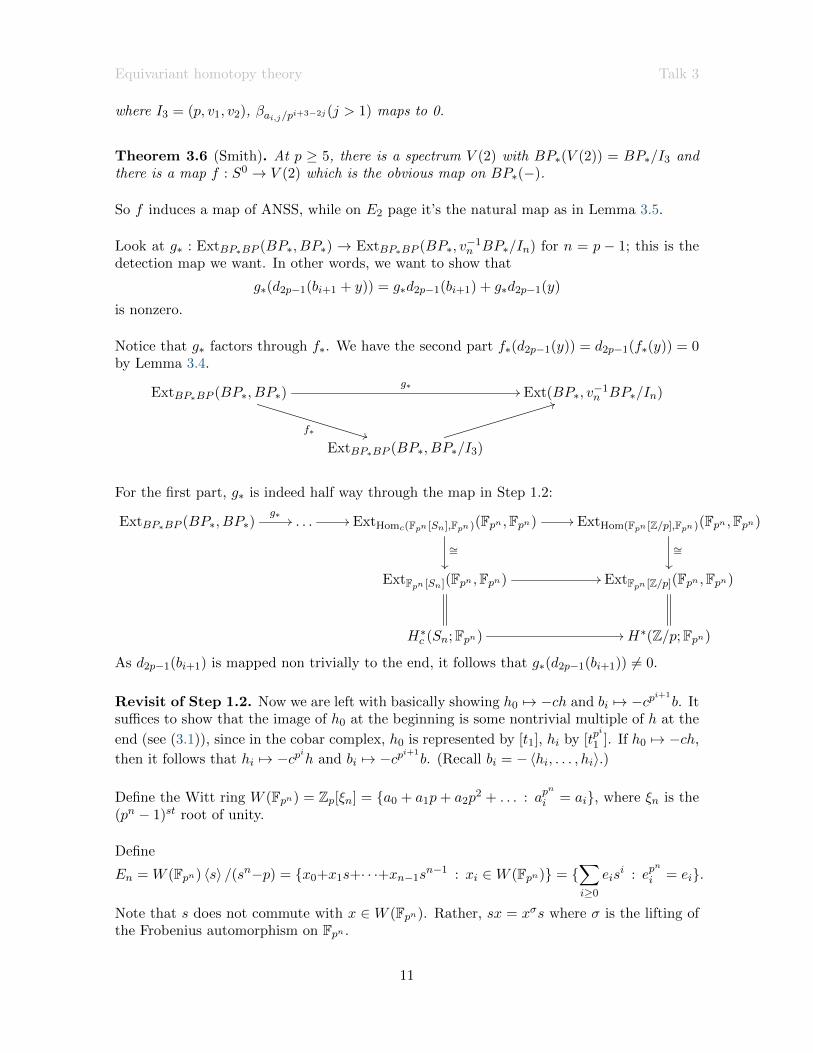
Theorem 3.6 (Smith). At p ≥ 5, there is a spectrum V (2) with BP∗(V (2)) = BP∗/I3 andthere is a map f : S0 → V (2) which is the obvious map on BP∗(−).
So f induces a map of ANSS, while on E2 page it’s the natural map as in Lemma 3.5.
Look at g∗ : ExtBP∗BP (BP∗, BP∗) → ExtBP∗BP (BP∗, v−1n BP∗/In) for n = p − 1; this is the
detection map we want. In other words, we want to show that
g∗(d2p−1(bi+1 + y)) = g∗d2p−1(bi+1) + g∗d2p−1(y)
is nonzero.
Notice that g∗ factors through f∗. We have the second part f∗(d2p−1(y)) = d2p−1(f∗(y)) = 0by Lemma 3.4.
ExtBP∗BP (BP∗, BP∗)g∗
//
f∗ **
Ext(BP∗, v−1n BP∗/In)
ExtBP∗BP (BP∗, BP∗/I3)
44
For the first part, g∗ is indeed half way through the map in Step 1.2:
ExtBP∗BP (BP∗, BP∗)g∗// . . . // ExtHomc(Fpn [Sn],Fpn )(Fpn ,Fpn) //
∼=
ExtHom(Fpn [Z/p],Fpn )(Fpn ,Fpn)
∼=
ExtFpn [Sn](Fpn ,Fpn) // ExtFpn [Z/p](Fpn ,Fpn)
H∗c (Sn;Fpn) // H∗(Z/p;Fpn)
As d2p−1(bi+1) is mapped non trivially to the end, it follows that g∗(d2p−1(bi+1)) 6= 0.
Revisit of Step 1.2. Now we are left with basically showing h0 7→ −ch and bi 7→ −cpi+1b. It
suffices to show that the image of h0 at the beginning is some nontrivial multiple of h at the
end (see (3.1)), since in the cobar complex, h0 is represented by [t1], hi by [tpi
1 ]. If h0 7→ −ch,
then it follows that hi 7→ −cpih and bi 7→ −cpi+1b. (Recall bi = −〈hi, . . . , hi〉.)
Define the Witt ring W (Fpn) = Zp[ξn] = a0 + a1p+ a2p2 + . . . : ap
n
i = ai, where ξn is the(pn − 1)st root of unity.
Define
En = W (Fpn) 〈s〉 /(sn−p) = x0+x1s+· · ·+xn−1sn−1 : xi ∈W (Fpn) =
∑i≥0
eisi : ep
n
i = ei.
Note that s does not commute with x ∈ W (Fpn). Rather, sx = xσs where σ is the lifting ofthe Frobenius automorphism on Fpn .
11

Equivariant homotopy theory Talk 4
Sn is the units of En congruent to 1 mod (s). In other words, there is an exact sequence1→ Sn → E×n → F×pn → 0.
The map in (3.1)
ExtBP∗BP (BP∗, BP∗)→ ExtHomc(Fpn [Sn],Fpn )(Fpn ,Fpn)→ ExtHom(Fpn [Z/p],Fpn )(Fpn ,Fpn)
is induced by a map of Hopf algebroid
(BP∗, BP∗BP )→ (Fpn ,Homc(Fpn [Sn],Fpn))→ (Fpn ,Hom(Fpn [Z/p],Fpn)).
The latter two are indeed Hopf algebras. More precisely, the first map is
BP∗BP → Homc(Fpn [Sn],Fpn))
ti 7→ (ti : 1 +∑
i>0 eisi 7→ ei), ei is the mod-p reduction of ei.
and the second map is by restricting to an order p subgroup of Sn.
First we show that t1 is not zero in Hom(Fpn [Z/p],Fpn). Take the generator x of Z/p inSn, such that xp = 1. Write x = 1 +
∑i>0 eis
n. We want to show e1 6= 0. Notice thatmod-p reduction being 0 is equivalent to being 0 itself. If e1 were zero, then we can expand(1+
∑i>0 eis
n)p = 1 and mod it out by ideals generated by some power of s. Inductively thiswould imply all the ei’s are zero, showing the x is of order 1, contradicting the assumptionthat x is of order p.
Second, we have Hom(Fpn [Z/p],Fpn) = Fpn [t]/(tp − t) where t is primitive. It is a fact thatt1 is primitive in Homc(Fpn [Sn],Fpn)). Since it is nonzero in the image, it has to be mappedto a nontrivial multiple of t.
As h0 is represented by [t1] and h by [t], it follows that h0 is mapped to a nontrivial multipleof h in (3.1). This completes the proof.
Talk 4: Review of category theory (Yexin Qu)
This talk is about Kan extensions, enriched categories, and Day convolutions.
4.1. Kan extension. Idea: suppose you have a functor F : C′ → E and a functor C′ → Cthat you should think of as “inclusion”, and you want to extend F to be a functor out of C.The Kan extension is the universal way to do this.
The definition is built up layer-by-layer. Let C, D, and E be categories, and let F : C → E andK : C → D be functors. If there exists L : D → E equipped with a natural transformationη : F =⇒ L K such that for all G : D → E equipped with a natural transformation toγ = F =⇒ G K there exists a unique α : L =⇒ G such that γ = α η. Call L the leftKan extension of F along K, and write LanK F .
C F //
K
⇓η
E
D
??
L
PP
G#α
12

Equivariant homotopy theory Talk 4
To get the right Kan extension, reverse all the arrows.
There is a right adjoint K∗ : ED → EC sending h 7→ h K, α 7→ γ = α η. So there is anisomorphism
ED(LanK−,−) ∼= EC(−,K∗−).
This is a local Kan extension. To define global Kan extensions, for all F ∈ EC , define K! tobe the left adjoint to K∗; this is the left Kan extension functor LanK −. The right adjointK∗ to K∗ is called the right Kan extension functor and denoted RanK −.
A functor F : C → Set is called corepresentable if there exists a natural isomorphism F ∼=hC : C → Set where h : c′ 7→ C(c, c′) for some c.
Example 4.1. The left Kan extension of
a→ b
↓c _
i
X // E
a → b
↓ ↓c → d
LaniX
EE
is the pushout of the diagram X.
A left Kan extension is a pointwise left Kan extension if it is preserved by all corepresentablefunctors: given corepresentable G in:
C F //
K
E G // Set
D
BB
LanK F
??
one has G LanK F = LanK G F .
4.2. Ends and coends. Let H : J op × J → C be a functor where J is small and Cis complete. For all f ∈ Mor(J ), f : j → j′ we have functors f∗ : Hom(j, j) → H(j, j′)and f∗ : Hom(j′, j′) → Hom(j, j′). We can generalize this by defining ϕ∗ : Hom(j, j) →∏
f∈MorJdom(f)=j
H(j, codomain(f)); then you get morphisms∏j∈J H(j, j)
ϕ∗→∏f∈MorJ (H,dom(f), codf)
and∏j′∈J H(j′, j′)
ϕ∗→∏f∈MorJ H(domf, codf).
Definition 4.2. An end∫J H(j, j) is the equalizer of∫
JH(j, j)→
∏j∈J
H(j, j)ϕ∗
⇒ϕ∗
∏f∈MorJ
H(domf, codf)
13
Equivariant homotopy theory Talk 4
if J is small and C is cocomplete. A coend∫ J
H(j, j) is the coequalizer of⊔f∈Mor(J )
H(domf, codf)ϕ∗
⇒ϕ∗
⊔j∈J
H(j, j)→∫ J
H(j, j).
Let C be small and E cocomplete. Then
LanK F (d) =
∫ JD(K(c), d) · F (c).
Here S · b =⊔s∈S b.
4.3. Monoidal categories.
Definition 4.3. A category C is monoidal if it has a binary operation ⊗, a unit object 1,and natural isomorphisms
αX,Y,Z : (X ⊗ Y )⊗ Z ∼= X ⊗ (Y ⊗ Z)
λ : 1⊗X ∼= X
ρ : X ⊗ 1 ∼= X
that satisfies some properties.
Definition 4.4. If a monoidal category C is symmetric, we also need a natural isomorphismTXY : X ⊗ Y ∼= Y ⊗X.
Definition 4.5. A monoidal category is called closed if for all X ∈ C, − ⊗ X has a rightadjoint. This is called the internal Hom, and written C(X,−).
For example, take the category of finite vector spaces with product as ⊕, unit object 0, andthe required morphisms as embeddings. This is not a closed monoidal category, because(0, C(X,Y )) 6∼= C(X,Y ).
If you don’t have an internal Hom, you might want to consider enriched categories.
4.4. Enriched categories. Let V = (V•,⊗, 1) be a symmetric monoidal category. Wesay that C is a V -category, or a category enriched over V , if
(1) there is a collection of objects in C;(2) for any X,Y ∈ ob C, an object V0 ∈ C(X,Y ), and 1→ C(X,X) ∈ MorV0;
(3) for all X,Y, Z ∈ ob C, there is a composition law
C(Y,Z)⊗ C(X,Y )→ C(X,Z).
4.5. Enriched functors. F : D → C is an enriched functor if F : obD → ob C, andD(X,Y )→ C(F (X), F (Y )).
14

Equivariant homotopy theory Talk 5
Definition 4.6. A V -natural transformation T : F =⇒ G if it assigns to an object X amorphism TX : 1→ C(F (X), G(X)) making the diagram commute:
D(X,Y )TY ⊗F //
G⊗TX
C(F (X), G(X))⊗ C(F (X), F (Y ))
C(G(X), G(Y ))⊗ C(F (X), G(Y )) // C(F (X), G(Y ))
4.6. Day convolution. Let D = (D0,⊕, 0) be a small, symmetric monoidal categoryenriched over V = (V0,⊗, 1) a cocomplete closed symmetric monoidal category. Let X,Y ∈[D, V ] (enriched functors D → V ). Let XY be the left Kan extension of the compositionof ⊗, X × Y along ⊕:
D ×D X×Y//
⊕##
V × V ⊗// V
DXY
55
This is a binary operation in [D,V ]. So ([D,V ],, I) where I : D → V sending D 7→Hom(0D, D).
Let D = JG be the category of finite-dimensional orthogonal representations (but the mor-phisms require some explanation), this is a symmetric monoidal category with product ⊕and unit 0. Let V = TG be topological G-spaces where the maps are not required to beequivariant. Applying this to that diagram with X,Y : JG → TG, we have
JG ×JG
⊕%%
X×Y// TG × TG ∧ // TG
JG
X∧Y
55
Talk 5: Equivariant homotopy theory I (J.D. Quigley)
RECALL: To build a CW complex, start by knowing how to add a cell by forming thepushout:
∂Dn ' Sn−1 fn// _
Xn−1
Dn // Xn
Maybe we want to add more than one cell, so we look at
Kn × Sn−1 fn//
_
Xn−1
Kn ×Dn // Xn
So here, fn is the attaching map, and Kn is a discrete set.
15

Equivariant homotopy theory Talk 5
We then have a sequence of inclusions K0 = X0 → X1 → X2 → . . . → colimnXn = X.
Definition 5.1. A G-CW complex is a CW complex as above where each Kn is a G-set, andeach fn is G-equivariant. Use the trivial action of G on Sn−1 and Dn.
Since Kn is a G-set, we can express it Kn =⊔i∈I G/Hi where Hi < G are defined up to
conjugacy. We say that G/Hi ×Dn is an n-dimensional G-cell.
Example 5.2. Let G = C2. Does S2 with the antipodal action have a G-CW structure?Think of this as compactified C with the sign representation, and first think of the CW com-plex structure with one point and a 2-disc attached. (This is not the regular representation.)This is G acting on a CW complex but is not a G-CW complex. (This is actually a problemfor a different reason – it doesn’t send the basepoint to itself.)
But we can build it up with a few more cells – use two 0-cells, two 1-cells between them, andtwo 2-cells between those. As a G-CW complex, this has K0 = K1 = K2 = G, and C2 actsby permuting cells.
Theorem 5.3 (Bredon). A G-equivariant map f : X → Y between G-CW complexes X,Y isan equivariant homotopy equivalence iff fH : XH → Y H is an ordinary homotopy equivalencefor all H ≤ G.
Remark/ Definition 5.4. H-equivariant homotopy of a G-space X is πH∗ (X) = π∗(XH).
Example 5.5 (another G-CW complex). Let P be a family of proper (closed) subgroupsof G. Define EP, the “universal space” for P, as the G-space (unique up to equivariantequivalence) satisfying EPG = ∅ and EPH is weakly contractible for all H ∈ P.
For example, if G = Cp, then attach G-cells G/H × Dn for all H ∈ P to make EPHweakly contractible. (This is described in a paper by Luck called “Transformation groupsand algebraic K-theory”.)
RECALL: A finite-dimensional orthogonal real representation of G is a group homomorphismπ : G→ O(V ) where V is a finite-dimensional Euclidean real vector space.
Example 5.6 (Sign representation). Let G = Cpn ⊂ Σpn . Then π(g)(v) = sgn(g) · v. Thisis a 1-dimensional representation. If p is odd, this is trivial.
Example 5.7 (Regular representation). Let G be finite, and let V = R[G]. Then π(g)(v) =π(g)(
∑g∈G rigi) =
∑gi∈G riggi.
Example 5.8 (Reduced regular representation). Use V = R[G]/ 〈g1 + g2 + · · ·+ gk〉 whereG = g1, . . . , gk. You could also define it as a subspace of R[G] where the coordinates sumto 0.
16

Equivariant homotopy theory Talk 6
Example 5.9. Let G = C2n have generator γ. Consider π : C2n → O(V ). This is determinedby π(γ) ∈ O(V ), i.e. a choice of orthogonal matrix A with A2n = I. If you thought aboutthis more (or looked it up on wikipedia) you’d believe that this can be written as a diagonal
matrix with R1, . . . , Rk,±1, . . . ,±1 on the diagonal, where Ri =
cos θ − sin θ
sin θ cos θ
. Pick θ
such that R2ni = I2. (Here θ ≡ 0 (mod 2π
2n ) but not π.)
We can put a partial ordering on these: say V1 < V2 if for every irreducible representation U ,we have dim HomG(U, V1) < dim HomG(U, V2)−1. Ignoring the −1, this says that V1 embedsequivariantly into V2; with the −1, it says that O(V1, V2)G is connected, i.e. all equivariantorthogonal embeddings are homotopic. (Here O(V1, V2)G means G-equivariant orthogonalembeddings.)
Let V be a G-representation. Its representation sphere SV has underlying space the one-point compactification of V with basepoint ∞, and the action is that G acts on V by therepresentation and acts trivially on ∞.
Let V, V ′ be G-representations, H < G, W an H-representation.
• SV⊕V ′ ∼= SV ∧ SV ′
• iGHSV = SResGH V where iGH : G-spaces→ H-spaces is the forgetful functor.
• SIndGH(W ) = T H(G+, SW ) =H-equivariant mapsG+ → SW where IndGH(W ) = R[G]⊗R[H]
W . H acts on G+ by left-multiplication, G acts on G+ by right-multiplication, and Gacts on T H(G+, S
W ) by left-multiplication on the source.
Let G = Cpn . We can give SV the structure of a G-CW complex as follows. Let G(i) to be the
index-pi subgroup of G. With this definition, we get a series of inclusions SVG
= SVG(0)
→SV
G(1)
→ . . . → SVG(n)
= SV|e = SV . G acts on SVG
trivially, so start by attaching asingle |V G|-cell.
Get SVG(i)
from SVG(i−1)
by attaching G/G(i) ×Dn for each |V G(i−1)< n ≤ |V G(i) |.
Example 5.10. Let V = sgn ⊕ sgn and G = C2. Then |V C2 | = |0| = 0 and |V C2 | = 0 <n ≤ 2. This is the same decomposition we had before (two each of 0-cells, 1-cells, 2-cells),but G acts trivially on the 0-cells.
If X is a G-space and V is a G-representation, πHV X = πH0 ΩVX = [SV ]H .
Talk 6: Introduction to equivariant homotopy theory II(Fei Xie)
Let V be a finite-dimensional real orthogonal representation of a finite group G (this is whatwe mean when we say “representation of G”).
17

Equivariant homotopy theory Talk 6
Definition 6.1. An orthogonal G-spectrum X is a collection of based G-spaces XV indexedby representations V of G with a non-equivariant action of O(V ). For an orthogonal inclusiont : V →W there is a structure map σ : SW−tV ∧XV → XW compatible with the orthogonalaction and the G-action.
Say that X is an Ω-spectrum if the adjoint maps σ : XV → ΩW−tVXW are all homeomor-phisms. (These are the fibrant objects.)
Notation 6.2. Let SG denote the category of G-spectra with equivariant maps.
Definition 6.3. For H ≤ G, the H-equivariant kth stable homotopy group of X is
πHk (X) = lim−→V >−k
πHV+k(XV )
(this uses the partial ordering in the last talk).
Definition 6.4. A stable weak equivalence (which we call just a weak equivalence) is a mapX → Y in SG inducing isomorphisms of πHk (−) for k ∈ Z, H ≤ G.
Recall there is a universal functor SG → hoSG sending weak equivalences to isomorphisms.The functor πHk (−) : SG → Ab takes weak equivalences to isomorphisms so it descends to a
functor πHk (−) = [Sk,−]H : hoSG → Ab.
Theorem 6.5. Let Xf be a fibrant replacement for X. Then πHk (X) = πk((Xf )H).
6.1. Isotropy separation sequence. Let F be a nonempty collection of subgroups ofG closed under passing to subgroups and conjugates. Such a collection is called a family ofsubgroups of G. There is a universal unbased G-space EF satisfying
(EF)H =
∗ H ∈ F∅ H /∈ F .
EF+ can be given a G-CW complex structure with cells of the form (G/H)+∧Dn for H ∈ F .
Let EF be the cofiber:EF+ → S0 → EF .
This satisfies:
(EF)H =
∗ H ∈ FS0 H /∈ F .
Let P be the family of all proper subgroups of G. Then the isotropy separation sequence is
EP+ ∧X → X → EP ∧X.We know that (G/H)+ ∧ − is adjoint to the restriction, so the LHS is determined by theaction of proper H. This can be used to prove things by induction on the order of the group.
18
Equivariant homotopy theory Talk 6
Definition 6.6. The geometric fixed point functor is
ΦG(X) = ((EP ∧X)f )G
where (−)f is fibrant replacement.
Remark 6.7. If X → Y is a map of cofibrant G-spectra EP ∧ X → EP ∧ Y is a weak
equivalence iff ΦG(X) → ΦG(Y ) is a weak equivalence. As an H-spectrum EP ∧ X is
contractible, so if H ≤ G is proper, then πH∗ (EP ∧ X) = 0 = πH∗ (EP ∧ Y ). (Note: EP iscontractible as an H-space and −∧X preserves homotopy equivalences as X is cofibrant, so
EP ∧X is also contractible as an H-space. Similarly for Y .)
Example 6.8. Let G = C2n . The space EP = EC2 ' S∞ with the antipodal action. The
G-action is through the epimorphism G C2. Then EP = limn→∞ Snσ where Snσ is the one-
point compactification of n copies of the sign representation. Let’s check this: if H is proper,then (S∞)H = (S∞)∗ = S∞ ' ∗, and (S∞)G = (S∞)C2 = ∅. Here S∞ = limn→∞ S(nσ).
6.2. Mackey functors.
Definition 6.9. A Mackey functor consists of a pair of functors M = (M∗,M∗) from the
category of finite G-sets to Ab such that:
• they have the same object function
• M∗ is covariant
• M∗ is contravariant
• they take disjoint unions to sums
• for a pullback diagram of finite G-sets
Sδ //
γ
A
α
Tβ// B
it gives a commutative diagram
M(S)δ∗ // M(A)
M(T )
γ∗
OO
β∗// M(B)
α∗
OO
Given a morphism Af→ B, call M∗(f) the restriction map and M∗(f) the transfer map.
Example 6.10. For a finite G-set B and X ∈ SG, homotopy groups
(πn(X))∗(B) = [Sn ∧B+, X]G
(πn(X))∗(B) = [Sn, B+ ∧X]G
19

Equivariant homotopy theory Talk 7
form a Mackey functor. They have the same object function because finite G-sets are self-dual. It is enough to know this for B = G/H. In this case,
πn(X)(G/H) = [Sn ∧G/H+, X]G = [Sn, X]H = πHn (X)
is the homotopy groups we defined earlier.
Given a Mackey functor M , there is an equivariant Eilenberg-Maclane spectrum HM suchthat
πn(HM) =
M n = 0
0 n 6= 0.
Definition 6.11. Equivariant homology is defined as
HGk (X;M) = πGk (HM ∧X)
and cohomology is defined as
HkG(X;M) = [X,ΣkHM ]G.
6.3. Constant and permutation Mackey functors. Let Z denote the Mackey func-tor represented by Z with trivial action. So Z(B) = HomG(B,Z) = Hom(B/G,Z). This isthe constant Mackey functor.
Let S be a G-set, and ZS be the free abelian group generated by S. Then the permu-tation Mackey functor on S is the Mackey functor represented by this, i.e. ZS(B) =HomG(B,ZS). Here restriction maps (−)∗ are given by pre-composition, and transfermaps (−)∗ are given by summing over fibers. (I.e. let g : A → B, for transfers, f gets sentto g∗(f)(b) =
∑x∈g−1(b) f(x).)
Let B be a G-set. Consider a free G-set G × B (where the action is trivial on B, and lefttranslation on G). Then the original action map G×B → B is equivariant. Automorphisms
of G × B over B are of the form (g, b)x7→ (gx, x−1b) for x ∈ G. It induces a G-action on
M(G×B) by (x−1)∗.
Lemma 6.12. Let B be a finite G-set, and M the permutation Mackey functor (on someG-set S). Then:
(1) Given an epimorphism B′ → B of finite G-sets, then M(B) → M(B′) ⇒ M(B′ ×B B′)is an equalizer.
(2) The action map G×B → B induces isomorphism M(B)→M(G×B)G.
(3) Given G→ G/H, there is an isomorphism M(G/H)→M(G)H .
(4) A map M →M ′ of permutation Mackey functors is an isomorphism iff M(G)→M ′(G)is an isomorphism (which is automatically G-equivariant).
Talk 7: Model categories I (Ugur Yigit)
20

Equivariant homotopy theory Talk 7
Definition 7.1. Given a commutative diagram
Af//
i
X
p
B
>>
g// Y
a lifting is a map h : B → X such that the resulting triangles are commutative.
If such lift exists for any f, g, say that i has the left lifting property w.r.t. p, and p has theright lifting property w.r.t. i.
Definition 7.2. A model category is a category C with the classes of maps:
(i) weak equivalences (w.e.)
(ii) fibrations (fib)
(iii) cofibrations (cof)
A map which is both a fibration [cofibration] and a weak equivalence is called an acyclic (ortrivial) fibration [cofibration].
We require the following axioms:
(MC1) C has all small limits and colimits.
(MC2) If f and g are maps such that fg is defined and if two of f, g, fg are weak equivalences,then so is the third.
(MC3) If f is a retract of g, and g is a weak equivalence, fibration, or cofibration, then so is f .
(MC4) Given a commutative diagram
Af//
i
X
p
B
>>
g// Y
a lifting exists in the following two cases:(i) i is a cofibration and p is an acyclic fibration
(ii) i is an acyclic cofibration and p is a fibration
(MC5) Any map f : X → Y can be factored in two ways:(i) f = pi where i is a cofibration and p is an acyclic fibration
(ii) f = pi where i is an acyclic cofibration and p is a fibration
and these factorizations are functorial.2
Using the axioms, you can prove that all three classes of maps contain all identities, and thatthey are closed under transfinite compositions. In a model category, we automatically havea terminal object ∗ and an initial object ∅.2Functoriality was not required by Quillen, but is typically required now, and all the interesting cases satisfythis. All factorizations gotten by the small object argument are functorial.
21
Equivariant homotopy theory Talk 7
Definition 7.3. An object A ∈ C is called cofibrant if the unique map ∅ → A is a cofibration,and fibrant if A→ ∗ is a fibrant.
Example 7.4. The category Top of topologial spaces can be given a model category structureby defining f : X → Y to be:
(i) a weak equivalence if it is a weak homotopy equivalence
(ii) a fibration if it is a Serre fibration3
(iii) a cofibration if it has the left lifting property w.r.t. all acyclic fibrations.
Note that the above definition of model categories is a bit over-determined: if you know theweak equivalences and cofibrations (or fibrations), you get everything else.
Proposition 7.5. Let C be a model category.
(1) The map i : A→ B is a cofibration iff it has LLP w.r.t. all acyclic fibrations;
(2) the map i : A→ B is an acyclic cofibration iff it has LLP w.r.t. all fibrations;
(3) the map p : X → Y is a fibration iff it has RLP w.r.t. all acyclic cofibrations;
(4) the map p : X → Y is an acyclic fibration iff it has RLP w.r.t. all cofibrations.
Be careful, though – if you define the weak equivalences and fibrations, there’s only onepossible choice of collection of cofibrations, but the resulting structure might not be a modelcategory.
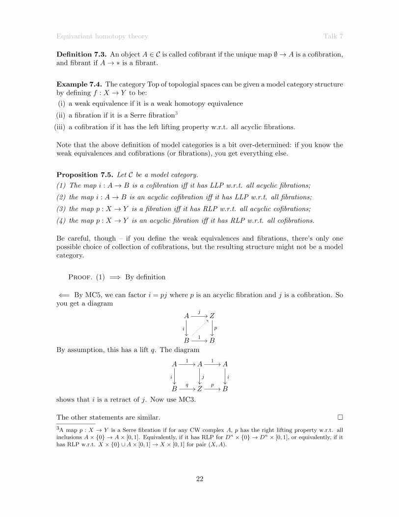
Proof. (1) =⇒ By definition
⇐= By MC5, we can factor i = pj where p is an acyclic fibration and j is a cofibration. Soyou get a diagram
Aj//
i
Z
p
B1 //
>>
B
By assumption, this has a lift q. The diagram
A1 //
i
A1 //
j
A
i
Bq// Z
p// B
shows that i is a retract of j. Now use MC3.
The other statements are similar. 3A map p : X → Y is a Serre fibration if for any CW complex A, p has the right lifting property w.r.t. allinclusions A× 0 → A× [0, 1]. Equivalently, if it has RLP for Dn × 0 → Dn × [0, 1], or equivalently, if ithas RLP w.r.t. X × 0 ∪A× [0, 1]→ X × [0, 1] for pair (X,A).
22

Equivariant homotopy theory Talk 7
Proposition 7.6. Let C be a model category. Two of the classes of weak equivalences,cofibrations, fibrations determine the third.
From (3) in the previous proposition, if we know the acyclic cofibrations, then we knowthe fibrations. By (4), if you know the cofibrations, you get the acyclic fibrations. A mapis a weak equivalence iff it can be factored as an acyclic cofibration followed by an acyclicfibration. So it suffices to specify the acyclic cofibrations and cofibrations. (You can makethe same statement for acyclic fibrations and fibrations but we like cofibrations.)
Instead of considering all [acyclic] cofibrations, we can consider generating [acyclic] cofibra-tions instead. The small object argument is a pain; I will concentrate on compactly generatedmodel categories.
From now on, we are working in a topological category (enriched in Top?).
Definition 7.7. An object A ∈ C is compact if given any · · · → Xn−1 → Xn → Xn+1 → . . . ,we have
colimn C(A,Xn) ∼= C(A, colimnXn).
Definition 7.8. We say that a class of maps J permits the small object argument in C if Cis cocomplete and the domains of the morphisms in J are compact.
Definition 7.9. A cofibrantly generated model category is a model category such that:
(1) There is set I of maps called generating cofibrations that permits the small object argu-ment and such that a map is an acyclic fibration iff it has the right lifting property w.r.t.all elements of I.
(2) There is a set J of maps called generating acyclic cofibrations that permits the smallobject argument and such that a map is a fibration iff it has the right lifting propertyw.r.t. J .
Example 7.10. In Top, we can take I = in : n ≥ 0 where in is the natural inclusionSn−1 = ∂Dn−1 → Dn, and J = jn : n ≥ 0 where jn is the map In → In+1 that is inclusionof the bottom face.
Let T G be the category of pointed topological G-spaces and equivariant maps.
Definition 7.11. An equivariant map f : X → Y is a naıve Serre fibration [weak equivalence]if f is a Serre fibration [weak equivalence] in T .
It is a genuine Serre fibration [weak equivalence] if fH : XH → Y H is a Serre fibration [weakequivalence] in T .
Theorem 7.12. In the naıve case, the sets
I ′G = in+ ∧G+ : n ≥ 0J ′G = jn+ ∧G+ : n ≥ 0.
23

Equivariant homotopy theory Talk 8
form a cofibrantly generated model category.
In the genuine case, use:
IG = in+ ∧G/H+ : n ≥ 0, H ⊂ GJG = jn+ ∧G/H+ : n ≥ 0, H ⊂ G.
You can also define model structures in between these by using the families in Fei’s talk.
Cofibrations are retracts of relative CW complexes.
This satisfies the pushout-product axiom w.r.t. the smash product.
These are monoidal model structures.
Talk 8: Model categories II (Alex Yarosh)
I’m going to tell you when a model category can fulfill its dream and be a cofibrantly generatedmodel category.
Definition 8.1. A category C is a homotopical category if it has a wide4 subcategory W
whose objects satisfy the 2 our of 6 property: if we have • f→ • g→ • h→ • where fg and hgare in W (“are equivalences”) then f, g, h, and hgf are in W .
This implies the 2 out of 3 property, by taking one of the maps to be the identity. It can beshown that the underlying category of a model category is a homotopical category.
Theorem 8.2 (Kan Recognition Theorem). Let M be a bicomplete5 homotopical categorywith sets of morphisms I, J that satisfy:
(1) I, J permit the small object argument.
(2) LLP(RLP(J)) ⊂ LLP(RLP(I)) ∩W where RLP(I) is the set of all maps that have theright lifting property w.r.t. all maps in I. (RLP(J) is the class of all fibrations; LLP ofthat is acyclic cofibrations. Similarly, LLP(RLP(I)) is cofibrations.)
(3) RLP(I) ⊂ RLP(J) ∩W .
(4) One of (2) or (3) is an equality.
Then M admits a cofibrantly generated model structure with I as the generating cofibrationsand J as the generating acyclic cofibrations.
Theorem 8.3 (Kan Transfer Theorem). Let M be a cofibrantly generated model category withI and J the generating cofibrations and acyclic cofibrations and N a bicomplete category. Alsoassume that there is an adjunction F : M N : U . Then if:
(1) FI, FJ both permit the small object argument
4W is wide if all objects are in W5has all limits and colimits
24
Equivariant homotopy theory Talk 8
(2) U takes relative FJ-cell complexes to weak equivalences
then N admits a cofibrantly generated model structure with FI and FJ as the generatingcofibrations and acyclic cofibrations, respectively. The weak equivalences in N are the mapsf such that Uf is a weak equivalence in M .
Definition 8.4. For a set of morphisms I, the subcategory of relative I-cell complexes is asubcategory of transfinite compositions of pushouts of maps in I: i.e.
X0 → X1 → · · · → Xβ → Xβ+1 → . . .
where each of these morphisms is a pushout of maps in I.
As the notation in the transfer theorem suggests, this is often used where U is a forgetfulfunctor and F is a free functor. So you can use this to put a model structure on a categorywith more structure.
New question: what if I have a model category but I don’t like it because the weak equiva-lences are not suitable for my purposes – for example, we might want to enlarge the class ofweak equivalences. This is what Bousfield localization is for.
From now on my model category M will be simplicial or topological, so I can talk abouthomotopy types of mapping spaces.
Definition 8.5. Let C be a class of morphisms. A fibrant object W is C-local if for any mapf : A → B in C, the induced map M(B,W ) → M(A,W ) is a weak equivalence. A mapg : X → Y is a C-local equivalence if for any C-local W , M(Y,W ) → M(X,W ) is a weakequivalence.
Definition 8.6. The (left) Bousfield localization of M at a class of morphisms C is a newmodel structure on M such that
(1) the weak equivalences are the C-local equivalences;
(2) the cofibrations remain the same;
(3) fibrations are defined by the right lifting property along trivial cofibrations.
Enlarging the weak equivalences and keeping the cofibrations the same means that there arefewer fibrations. Note that this isn’t a guarantee that this exists!
Sometimes “Bousfield localization” is the name of a functor LC from M with the old modelstructure to M with the new model structure. We also have a natural transformation η :1→ LC such that LC(X) is C-local and X → LCX is a C-equivalence.
Example 8.7 (Localization of spaces w.r.t. a homology theory h∗). If h∗ = H(−,Z/p)then localization w.r.t. h∗ is p-completion. If h∗ = H(−,Z(p)) then localization w.r.t. h∗ isp-localization.
Definition 8.8. We define the strict model structure on simplicial spectra as follows:
25

Equivariant homotopy theory Talk 9
• f : X → Y is a weak equivalence if fn : Xn → Yn is a weak equivalence.
• f : X → Y is a fibration if fn : Xn → Yn is a fibration.
• f : X → Y is a cofibration if f0 : X0 → Y0 and induced maps Xn+1⊔
ΣXnΣYn → Yn+1
for n ≥ 0 are cofibrations.
Definition 8.9. We define the stable model structure on simplicial spectra as follows. Assumethere’s a functor Q : sSp → sSp and a natural transformation η : 1 → Q such that QX isan Ω-spectrum for all X and QX → QQX is a weak equivalence. (For example, (QX)n =lim−→ Sing Ωi|Xn+i|.)• f : X → Y is a weak equivalence if f∗ : πnX → πnY is an isomorphism
• f is a stable cofibration if it’s a strict cofibration.
• f is a stable fibration if: f is a strict fibration
the diagram
Xn//
(QX)n
Yn // (QY )n
is a homotopy pullback.
Example 8.10. Localize Top∗ w.r.t. f : Sn+1 → ∗ for a fixed n?. Local objects are thoseX that have Ωn+1X contractible. (Or equivalently, πk(X) = 0 for k ≥ n+ 1.)
Then the localization of X is the nth Postnikov section of X.
Theorem 8.11. If S is a set and M is either left proper and cellular6 or left proper7 andcombinatorial8, then the Bousfield localization exists.
You can construct the localization functor by fibrant replacement.
Talk 9: The Mandell-May definition of G-spectra (ReneeHoekzema)
9.1. Motivation. A classical spectrum is a sequence of spaces En with structure mapsσ : ΣEn → En+1. Let’s rephrase this in a way that’s useful: let N be the category thathas objects n ∈ N and morphisms only identities. This is a symmetric monoidal category:the product sends (n,m) 7→ n + m and on morphisms, (1n,1m) 7→ 1n+m. Consider SN ∈Fun(N,Top∗) sending n 7→ Sn. I can trivially view this as a topologically-enriched category,where n is a point. This has a monoidal structure with Day convolution.
6“like Top”7“like sSet”8a model category is left proper if the pushout of a weak equivalence along a cofibration is a weak equivalence
26

Equivariant homotopy theory Talk 9
Definition 9.1. A spectrum is a functor E : N→ Top∗ that is a module for SN.
The problem is that SN is not a commutative monoid, and so SN-modules do not form asymmetric monoidal category. By “modules for SN”, I mean it has an action En∧Sm → En+m
such that the following diagram commutes:
En ∧ Sk ∧ S` //
σ
En ∧ Sk+`
σ
En+k ∧ Sk // En+k+`
Commutativity is commutativity of the following diagram
SN ⊗ SN
τ
µ
$$
SN
SN ⊗ SNµ
::
On objects, this is
Sn ∧ Sm
τ
// Sn+m
Sm ∧ Sn
99
In the top map, the n basis vectors in the Rn that is compactified to form Sn get sent to thefirst n basis vectors from Sn+m. Going the other way around, the n basis vectors from Sn
are sent to the last n basis vectors from Sn+m. This doesn’t commute!
Obviously, these things are related by a basis permutation map Sn+m → Sn+m.
Actually, you only need commutativity up to isomorphism. So the diagram you really wantto commute is
SN ⊗ SNτ
µ// SN∼=
SN ⊗ SN µ// SN
and the problem is that in this category we don’t actually have the requisite nontrivial au-tomorphism of SN (due, of course, to lack of good automorphisms of N in this category).
9.2. Orthogonal spectra. Let O be the category whose objects are n ∈ N and whosemorphisms are given by Hom(n, n) = O(n) and Hom(n,m) = ∅ for n 6= m. This is symmetric
27

Equivariant homotopy theory Talk 9
monoidal: again, the map on objects is (n,m) 7→ n + m, and on morphisms, the pair (f, g)
for f ∈ O(n) and g ∈ O(m) gets sent to the transformation
f 0
0 g
∈ O(n+m).
Again consider SO ∈ Fun(O,Top∗) sending n 7→ Sn. Now, the symmetric structure onFun(O,Top∗) by Day convolution incorporates both X ∧ Y ↔ Y ∧X, and switching f and
g in
f 0
0 g
.
What does this Day convolution do? Remember it’s the dotted arrow in
O ×O //
+
Top∗×Top∗−∧−
// Top∗
O
33
Definition 9.2. An orthogonal spectrum is a functor E : O → Top∗ that is a module forSO.
Definition 9.3. We define a category J whose objects are vector spaces V with innerproduct. The morphisms are. . . a little complicated. First consider O(V,W ), the Stiefelmanifold of orthogonal embeddings V → W . Let ϕ ∈ O(V,W ). Take the orthogonalcomplement W − ϕ(V ) for each ϕ; this defines a vector bundle on O(V,W ), where overevery embedding sits the orthogonal complement of that embedding. Now define J (V,W )to be the Thom space of this vector bundle.
This is symmetric monoidal: on objects, the product sends (V,W ) 7→ V ⊕W and on mor-phisms there is a composition J (V,W ) ∧J (V ′,W ′) → J (V ⊕ V ′,W ⊕W ′) and a com-position J (V,W ) ∧J (U, V ) → J (U,W ) that I won’t define. Also, it’s enriched overTop∗.
Let’s re-define orthogonal spectra.
Definition 9.4. An orthogonal spectrum is a functor E : J → Top∗ sending V 7→ EV . Onmorphisms, there’s a map J (V,W )→ Hom(EV , EW ). The Hom-tensor adjunction in Top∗gives structure maps εV,W : J (V,W ) ∧ EV → EW .
For example, J (Rn,Rn+1) is the Thom space of the bundle E → O(n, n+ 1) with fiber R1,and that is
∨O(n,n+1) S
1. So J (Rn,Rn+1) ∧ ERn =∨ϕ ΣϕERn → ERn+1 .
9.3. The sphere spectrum and Yoneda spectra. (I write S instead of S to emphasizethat it’s a spectrum.) The sphere spectrum S−0 : V 7→ SV is the Thom space of V → ∗which is J (0, V ). More generally, S−V : W 7→ J (V,W ). These are the representablefunctors – the image of the enriched Yoneda embedding J op → Fun(J ,Top∗) sendingV 7→ HomJ (−, V ) = J (V,−).
28

Equivariant homotopy theory Talk 9
Lemma 9.5 (Enriched Yoneda lemma). HomSp(S−V , E) = EV
9.4. Towards G-spectra. Let G be a finite group. Let T G be the category whoseobjects are based G-spaces and whose morphisms are equivariant continuous maps.
Let TG be the category whose objects are based G-spaces and whose morphisms are allcontinuous maps. This is the category we’ll be interested in. It has a G-action: given somef : X → Y then we’ll define the action of γ as the composition:
Xf// Y
γ
X
γ−1
OO
Y
Now I’m going to adapt my indexing category to also have something to do with G.
Definition 9.6. The Mandell-May category is the category JG whose objects are orthogonalrepresentations of G. To define the morphisms, do the same thing as before; note thatO(V,W ) has all orthogonal embeddings V →W , not just equivariant ones.
Definition 9.7. An (orthogonal) G-spectrum is a functor E : JG → TG, sending V 7→ EV .
9.5. Naıve vs. genuine G-spectra. There is an embedding Ji→ JG by taking
trivial representations – whatever G is, every vector space is present here because it has a
trivial representation. It’s also a full subcategory. So if I have a functor JGE→ TG then you
compose to get a functor J → TG. Such a functor is called a naıve G-spectrum. It is justan orthogonal spectrum with a G-action.
A functor from JG is completely determined by its value on J . The categories are equivalentas Top∗-enriched categories, but the natural model structure you put on them is different.Why are they equivalent? Consider the structure maps εV,W : J (V,W )∧EV → EW , whichfactors over JG(V,W )∧O(V )EV . If dimV = dimW , then J (V,W )∧O(V )EV = O(V,W ) ∼=EW . So the functor is completely determined by what it does on the trivial representations.
An equivariant map that is an underlying homeomorphism is an equivariant homeomorphism.
9.6. Spectra and spaces. Given a spectrum F and a G-space X, define E ∧X : V 7→EV ∧X. If X = SW then E ∧SW is denoted ΣWE. Define FG(X,E) : V 7→ HomT G(X,EV ).If X = SW , then FG(SW , E) is denoted ΩWE.
9.7. Tautological presentation. Any spectrum E is the reflexive coequalizer of (i.e.colimit of the diagram) ∨
V,W S−W ∧JG ∧ EV//
//
∨V S−V ∧ EVoo
29

Equivariant homotopy theory Talk 10
The forward maps are jV,W ∧ EV and S−W ∧ εV,W and the backwards map is the obvious
inclusion. Abbreviate this as follows: lim−→V
S−V ∧ EV .
9.8. Smash product of spectra. We want to define the smash product given the Dayconvolution, and the Day convolution was the Kan extension of the following diagram
JG ×JGE×F
//
⊕
TG × TG // TG
JG
44
E ∧ F = lim−→V,W ′
S−V⊕V ′ ∧ EV ∧ FV ′ , i.e. the reflexive coequalizer of
∨V,V ′,W,W ′ S−W⊕W
′ ∧JG(V,W ) ∧J (V ′,W ′) ∧ EV ∧ FV//
//
∨S−V⊕V ′ ∧ EV ∧ FV ′oo
The category of G-spaces and all maps is a closed monoidal category, but the category ofG-spaces and equivariant maps is not closed.
Talk 10: The homotopy category of SG (Allen Yuan)
A homotopical category is a category C plus a class of weak equivalences W (satisfying thetwo-of-six condition). There is a functor C → ho C, where ho C = C[W−1] is just invertingthe weak equivalences. This talk will be about ho C, and what we can say about it withoutactually putting a model structure on it.
Definition 10.1. For any category A, a homotopy functor C → A is one that takes weakequivalences to isomorphisms. By the universal property of localization, this means it factorsthrough the homotopy category
C //
!!
ho C
A.
The analogous notion for functors between two homotopical categories is:
Definition 10.2. A functor F : C → D is homotopical if it takes weak equivalences to weakequivalences. As such, it induces the following diagram:
C F //
D
ho C F // hoD.
Thus, the study of functors on the homotopy category is equivalent to finding and studyinghomotopical functors upstairs.
30

Equivariant homotopy theory Talk 10
Goals:
(1) Determine if functors are homotopical.
(2) If not, determine a homotopically wide9 subcategory C ⊂ C
C //
C
ho C ∼ // ho Con which the functor is homotopical.
Some motivation:
Definition 10.3. The Spanier-Whitehead category SWG is the category whose objects arefinite G-CW complexes and whose morphisms are SWG(X,Y ) = colimV [SV ∧X,SV ∧ Y ]G.
Pros:
• the objects are pretty easy to work with; it’s easy to get a fuss-free smash product. Soit’s symmetric monoidal.
• can add formal desuspensions.
• Spanier-Whitehead duality.
Cons:
• It’s too small: no small limits and colimits. Analogy: think about finite-dimensionalvector spaces – they are the fully dualizable objects in the category of all vector spaces,but there are no small colimits. This isn’t good enough. For example, you can’t hope toget a model structure.
Our goal is to produce an embedding of SWG into hoSG that is fully faithful and a symmetricmonoidal embedding. There are some things we want this to satisfy:
• (Additivity) We need ∨ and finite∏
to be homotopical functors, and we want∨i∈I Xi '∏
i∈I Xi if I is a finite set. (For example, Sn×Sn = Sn ∨Sn ∪S2n and stably S2n → S∞
which is contractible, so S × S ' S ∨ S.)
• (Stability) We want − ∧ SV and − ∧ S−V to be inverse equivalences on hoSG.
• (Monoidal structure) We want hoSG to be symmetric monoidal under ∧.
10.1. Additivity. We want to show π∗(X ∨Y ) = π∗X⊕π∗Y . Normally, you get a LESof cofiber sequences, and get a splitting of that. The key to getting a LES here is that the(co)tensor on SG is levelwise. So you can define F := X×Y PY (fiber) and Y ∪CX (cofiber)levelwise.
Proposition 10.4. For all H ⊂ G, get a long exact sequence:
· · · → πHk F → πHk X → πHk Y → πHk−1F → . . .
9C ⊂ C is homotopically wide if every object in C is weakly equivalent to something in C.
31

Equivariant homotopy theory Talk 10
Proof. Fiber sequences are defined levelwise and stuff commutes with colimits.
colimV (πHk+V FV → πHk+VXV → . . . )
For a cofiber sequence we want a similar LES.
Remark 10.5. If Z ∈ SG there exists a fiber sequence ZY ∪CX → ZY → ZX . Takinghomotopy groups gives you the usual long exact sequence associated to a cofiber sequence.However, we want one with mapping INTO a cofiber sequence - this is the usual property ofa stable category.
Proposition 10.6. For Z ∈ SG, get a long exact sequence
· · · → [Z,X]→ [Z, Y ]→ [Z, Y ∪ CX]→ . . .
Proof. You haveZ //
β
CZ
Y // Y ∪ CXand you want to get the map α in
Z= //
α
Z //
β
CZ
X // Y // Y ∪ CXExtend this to
Z //
α
Z //
CZ //
ΣZ
ϕ
// ΣZ
Σβ
X // Y // Y ∪ CX // ΣX // ΣY
Then claim that ϕ = Σα.
Lemma 10.7. There is a natural isomorphism πH∗ X∼= πHk+1ΣX.
We want Y ∪ CX ' Y/X. In spaces, this happens for h-cofibrations, and those participatein the Hurewicz model structure.
Definition 10.8. An h-cofibration is a map i : A → X in SG such that for all f : X → Y
and homotopy H : A ∧ I+ → Y there exists a homotopy H : X ∧ I+ → Y .
Proposition 10.9. h-cofibrations in SG are objectwise closed inclusions.
Corollary 10.10. If f : X → Y is an h-cofibration, then you get a LES
· · · → πHk (X)→ πHk (Y )→ πHk (Y/X)→ . . . .
32

Equivariant homotopy theory Talk 10
Corollary 10.11. For all H ⊂ G:
(1) For any collection Xα ⊂ SG,⊕πH∗ (Xα) = πH∗ (
∨Xα).
(2) If Xα is finite, then∏πH∗ (Xα) = πH∗ (
∏Xα). This follows from the fact that the
unstable homotopy groups commute with products.
(3) If Xα is finite, then the natural map∨Xα →
∏Xα is a weak equivalence.
Corollary 10.12. hoSG is an additive category. Furthermore, the coproduct is computed as∨, and finite products are
∏.
How you get this is to use that these are the adjoints of the diagonal map, the diagonal mapis homotopical, and things descend properly.
10.2. Showing that −∧SV , −∧S−V are inverse equivalences on hoSG. First, weneed to show that these are homotopical. Do this later.
We know how to define S−V ∧ SV ∧X, and we want to show it’s weakly equivalent to X.
Example 10.13. In the non-equivariant case, look at S−1 ∧ S1 vs. S0. These are not thesame spectrum: (S0)n = Sn but (S−1 ∧S1)n = J (1, n)∧S1 = Thom(O(1, n),Rn\R)∧S1 =Thom(T (Sn−1)) ∧ S1. When you add the tangent bundle to the normal bundle, you get atrivial bundle. So this is Thom(Rn ↓ Sn−1) = Σn(Sn−1
+ ) = Sn ∨ S2n−1 and the second factordies stably.
If t : V →W is an embedding, we get a map S−W ∧SW → S−V ∧SV . The previous argumentworks in this case, too.
We constructed SG → hoSG but we don’t know how to access the morphisms in this homo-topy category. Let’s approximate it instead. One thing to try is that you can look at π0SG.This has the advantage that it’ll still detect weak equivalences.
But we would want to show that S−V ∧SV ∧X ' X, so instead, we’re going to create a slightlytweaked category πstSG that is rigged to have this property. πstSG is the category whoseobjects are the objects of SG, but the morphisms are πstSG(X,Y ) = colimV π0SG(S−V ∧SV ∧X;Y ).
Recall: for H ⊂ G, we had πHn (X) = colimV πHn+V (XV ). The stable weak equivalences are
maps f : X → Y inducing isomorphisms on πHn for all H ⊂ G, n ∈ Z.
This approximating category πstSG still sees weak equivalences:
Proposition 10.14. πstSG(G/H+ ∧ Sk, Y ) = πHk (Y )
This says that if two things are isomorphic in πstSG then they have to be weakly equivalent.Maps from G/H+∧Sk is the same as πH(−). One thing that’s really nice about this categoryis that it’s easy to calculate maps in it.
33

Equivariant homotopy theory Talk 10
Proof. Using the Yoneda property that SG(S−V ∧A, Y ) = T G(A, YV ), we can turn thisinto a statement about spaces: colimV π0SG(S−V ∧SV ∧G/H+∧Sk, Y ) = colimV π0T G(SV ∧G/H+ ∧ Sk, Y0). But this is colimV π0T H(SV ∧ Sk, YV ) = πHk (Y ).
(Recall SG is the category of G-spectra with equivariant maps, enriched over Top∗.)
Proposition 10.15. S−V ∧ SV ∧X → X is an equivalence in hoSG.
We want to show that − ∧ SV and − ∧ S−V are inverse equivalences on hoSG. The onlything we’re missing is that they’re actually functors on hoSG, so we want to show that they’rehomotopical.
Remark 10.16. The fact that these are inverse equivalences over πstSG gives you a tensorover the Spanier-Whitehead category. We can rewrite πstSG(X,Y ) = colimV π0SG(SV ∧X,SV ∧ Y ) so for finite G-CW complexes, there is an inclusion SWG(K,L) → πstSG(K,L)and so πstSG is tensored over SWG.
As a consequence, you get duality. If J is a finite G-set, πstSG(Z, J+ ∧ X) = πstSG(J+ ∧Z,X) = πstSG(Z,
∏GX). If you do more work, you can amp this up to arbitrary indexed
wedges, but we won’t do that.
Now we’re back to showing that −∧SV and −∧S−V are homotopical. Recall πstSG(G/H+∧Sk,−) = πHk (−) so this is a homotopy functor. The LES gives an argument to build things
up with cells, so you can show that πstSG(S` ∧K,−) is homotopical, for K a finite G-CWcomplex and ` ∈ Z. In particular, πstSG(G/H+ ∧ Sk ∧ SV ,−) is homotopical. By duality,this is the same thing as πstSG(G/H+∧Sk, S−V ∧−) = πHk (S−V ∧−) so that is homotopical.
This is just the homotopy groups, so that means S−V ∧− is homotopical. Since SV and S−V
are inverse on the approximating category, − ∧ SV is also homotopical.
Corollary 10.17. − ∧ SV and − ∧ S−V are inverse equivalences on hoSG.
Proposition 10.18. We’ve shown that πstSG(S−V ∧K,−) is homotopical. Duality says that− ∧ S−V ∧K is homotopical.
Now we can say something about how good the approximation is.
πstSG is a homotopical category using the weak equivalences in SG. This gives an equivalenceof categories hoSG ∼→ hoπstSG. The key idea is that, for a homotopical category C, you geta natural transformation C(X,−) → ho C(X,−). The LHS is a homotopy functor and theRHS isn’t. But this is the initial natural transformation from the Yoneda functor C(X,−)to a homotopy functor. So the Yoneda functor in the homotopy category is the closesthomotopical functor to C(X,−) from the right.
This means in particular that if C(X,−) were homotopical to begin with, then the twofunctors would be equal. This looks bothersome, but this condition is just never satisfied ine.g. actual G-spectra. But it is satisfied for our approximating category.
34

Equivariant homotopy theory Talk 10
So when πstSG(X,−) is homotopical, we have hoSG(X,Y ) = hoπstSG(X,Y ) = πstSG(X,Y ),and this is good because we know how to calculate the thing on the right.
In particular, when X,Y are finite G-CW complexes, then hoSG(X,Y ) = colimV π0SG(XV ∧X,SV ∧ Y ) = SWG(X,Y ). So we’ve shown:
Corollary 10.19. Σ∞ : SWG → hoSG is fully faithful.
Remark 10.20. (This is a property of the homotopy category that I’m not going to prove.)Any X ∈ SG has a “canonical homotopy presentation”; that means you can write
X = hocolim(· · · → S−Vn ∧XVn → S−Vn+1 ∧XVn+1 → . . . )
where Vn is an exhaustive sequence and XVn is a G-CW complex.
10.3. Smash product. ∧ is not known to be homotopical in general. But sometimesit is. . .
Definition 10.21. X is flat if − ∧X is homotopical.
We’ve shown that S−V ∧K is flat. Now you should believe that this is a big enough class ofobjects that you can do the small object argument and get flat approximations.
Proposition 10.22. If X ∈ SG, there exists a functorial weak equivalence X∼→ X where X
is flat.
For example, a cofibrant-fibrant approximation of anything is going to be flat. Cofibrantapproximation in any of the model structures Hood will talk about is flat.
Let SGfl ⊂ SG be the full subcategory of flat objects. Then you get an equivalence of categories
hoSGfl∼→ hoSG. This is the homotopically wide subcategory I mentioned at the beginning.
Proposition 10.23. Let X,Y be flat, and Z any spectrum. If you have a weak equivalenceX∼→ Y then Z ∧X → Z ∧ Y is a weak equivalence.
Proof.
X ∧ Z //
X ∧ Z
Y ∧ Z // Y ∧ ZThe top and bottom maps are weak equivalences. Smashing with Z is homotopical, so theleft vertical map is a weak equivalence.
Corollary 10.24. ∧ is a homotopical functor SGfl × SG → SG. This gives you ∧ : hoSG ×hoSG → hoSG.
35
Equivariant homotopy theory Talk 11
Corollary 10.25. Σ∞ : SWG → hoSG is fully faithful and symmetric monoidal.
Talk 11: The positive complete model structure and whywe need it (Hood Chatham)
Allen told us in his talk about what information we can get about the homotopical structureof SG directly. In particular, he built the homotopy category by “bare hands”. However, wehave a large number of functors that we care about, both on SG, and importantly on thecategory of rings commG. Most of these functors are not homotopical on the whole categoryof SG. In order to get these functors to behave well, they need to be derived. Thus, we wantto find some appropriate model structure on SG for which the various functors we care aboutare homotopical on maps between cofibrant objects so that we can use cofibrant replacementto derive them. In particular, we want a monoidal cofibrantly generated model structure onSG such that:
(1) The weak equivalences are the stable equivalences
(2) The Kan Transfer Theorem applies to the adjunction SGSym
// commG
Uoo
(3) If f is a cofibration or trivial cofibration then so is ΦH(f) for all H ⊆ G.
(4) Many other things we don’t explicitly have to worry about: cofibrant replacement shouldderive all of our favorite functors.
I should note at this point that (2) is the condition that is most important and will requirethe most work. It has nothing in particular to do with equivariant homotopy theory – thistalk would be almost the same even if we were only interested in nonequivariant ring spectra.Condition (3) is the source of a minor modification to the model structure that explicitlyrelates to equivariantness.
Recall that a model category is a category with specified classes of cofibrations, fibrations,and weak equivalences satisfying the following conditions:
(1) All three classes are closed under composition and retracts.
(2) If two of f , g, and gf are weak equivalences, then so is the remaining.
(3) Call a morphism a trivial cofibration (resp triv. fibration) if it is a cofibration (resp.fibration) and a weak equivalence. Given a class C of morphisms, write LLP(C) for theset of maps with the left lifting property against elements of C and RLP(C) for the setof maps with the right lifting property against elements of C. We should have:(a) RLP(cofibrations) = trivial fibrations
(b) RLP(trivial cofibrations) = fibrations
(c) LLP(fibrations) = trivial cofibrations
(d) LLP(trivial fibrations) = cofibrations
(4) Every map can be factored either as a trivial cofibration followed by a fibration or as acofibration followed by a trivial fibration.
Note that if you write down two of the three classes of cofibrations, fibrations, and weak equiv-alences, there is at most one model structure with these classes as specified: for instance, ifwe have cofibrations and weak equivalences, the fibrations must be RLP(trivial cofibrations).
36
Equivariant homotopy theory Talk 11
If cofibrations and fibrations are given, then we know the trivial cofibrations and trivial fi-brations too. Any weak equivalence may be factored as a trivial cofibration followed by afibration, and by two of three the fibration must be a weak equivalence too, so we get theclass of weak equivalences by taking compositions of any trivial cofibration followed by anytrivial fibration. Note that not any pair of classes satisfying conditions (1) and (2) gives riseto a third collection that makes a model category – condition (3) need not be satisfied.
In general, there can be set theoretic problems in constructing the factorizations for condition(4). The concept of a cofibrantly generated model structure is designed to ensure that ourmodel category can be defined using a set-theoretically small amount of data, which allowsus to use the small object argument to show that condition (4) is satisfied, and also allowsus to use a large collection of tools that only work on cofibrantly generated model categories,most importantly for this talk, the Kan Transfer theorem.
Recall that a cofibrantly model category is a category with two specified sets, the set I ofgenerating cofibrations, and the set J of generating trivial cofibrations. These need to satisfy:
(1) I and J admit the small object argument (so there exists some cardinal κ such that allthe domains of maps in I and J are κ-small)
(2) Write cofib(S) for LLP(RLP(S)). Set cofibrations = cofib(I), fibrations = RLP(J ),trivial cofibrations = cofib(J ), and trivial fibrations = RLP(I). Set the weak equiva-lences to be compositions of trivial cofibrations with trivial fibrations. These classes mustsatisfy condition (3) for model categories, and also we must have that trivial (co)fibrations =(co)fibrations ∩ weak equivalences.
These conditions are sufficient for these collections to be the collections of cofibrations, fi-brations, and weak equivalences of a model category. This statement is called the KanRecognition theorem. Note that in our case, we will be dealing with topological model cat-egories, and all the domains of all of the maps in I and J will always be compact, so theywill always admit the small object argument.
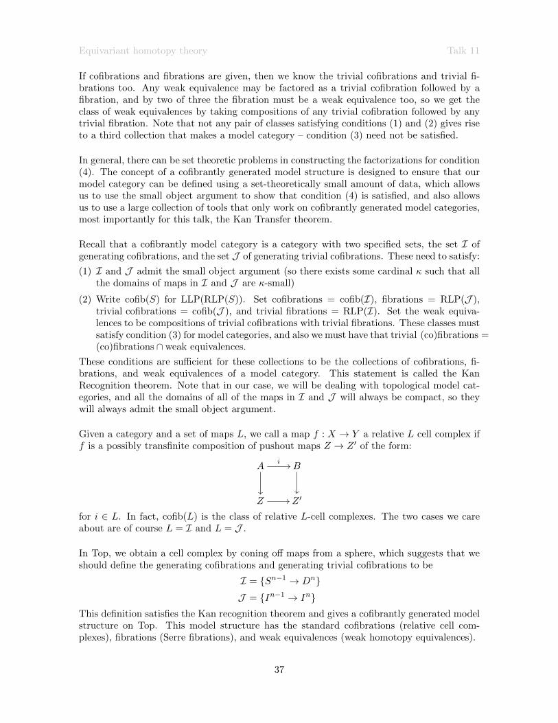
Given a category and a set of maps L, we call a map f : X → Y a relative L cell complex iff is a possibly transfinite composition of pushout maps Z → Z ′ of the form:
A
i // B
Z // Z ′
for i ∈ L. In fact, cofib(L) is the class of relative L-cell complexes. The two cases we careabout are of course L = I and L = J .
In Top, we obtain a cell complex by coning off maps from a sphere, which suggests that weshould define the generating cofibrations and generating trivial cofibrations to be
I = Sn−1 → DnJ = In−1 → In
This definition satisfies the Kan recognition theorem and gives a cofibrantly generated modelstructure on Top. This model structure has the standard cofibrations (relative cell com-plexes), fibrations (Serre fibrations), and weak equivalences (weak homotopy equivalences).
37

Equivariant homotopy theory Talk 11
Now I will make an analogue for SG; this will be the complete level model structure. We set
I = G+ ∧H S−V ∧ (Sn−1+ → Dn
+) : H ≤ G and V an H-repJ = G+ ∧H S−V ∧ (In−1
+ → In+) : H ≤ G and V an H-repHere “complete” means that H is allowed to range over the complete family of all subgroupsof G (rather than some smaller family). The word “level” is a synonym for “strict,” whichwas the term used yesterday. It refers to the weak equivalences – it turns out that the weakequivalences we get for this model structure are the levelwise weak equivalences: they arethe maps f : X → Y of spectra such that fV : XV → YV is a weak equivalence of G-spacesfor all G.
Let’s demonstrate that the levelwise equivalences are the class of weak equivalences we getfor the cofibrantly generated model structure on SG specified by this I and J . Note thatall elements of I and J are levelwise weak equivalences. This implies that all relative Jcomplexes are levelwise weak equivalences. We just need to check that all trivial fibrationsare levelwise weak equivalences too.
The trivial fibrations are given by RLP(I). Such a trivial fibration needs to admit a lift forall diagrams of the form:
G+ ∧H SV ∧ Sn+1+
//
X
G+ ∧H S−V ∧Dn+
// Y
which is equivalent by the adjunction between G+ ∧ − and ResGH to admitting a lift for alldiagrams of the form:
S−V ∧ Sn−1+
//
ResGH X
S−V ∧Dn+
// ResGH Y
Now using the adjunction between S−V ∧ : TopG∗ → SG to get S−V to the other side:
Sn−1+
//
(ResGH X)V
Dn+
// (ResGH Y )V
Now asking for a map Z → W of pointed spaces to admit all lifts of this form implies thatZ →W is a trivial fibration. We see that XV → YV is a weak equivalence for all V and henceX → Y is a levelwise weak equivalence. Since every weak equivalence is the composition ofa trivial cofibration with a trivial fibration and both trivial cofibrations and trivial fibrationsare levelwise weak equivalences, we deduce that the weak equivalences are exactly the set oflevelwise weak equivalences.
So we get the levelwise model structure. This isn’t so nice because we care about stable things.If we can make the maps eV,W : S−(V⊕W ) ∧ SV → S−W into weak equivalences, this will getus our stable complete model structure. We have the most direct control over generatingtrivial cofibrations, which all must be weak equivalences, so our approach will be to add the
38
Equivariant homotopy theory Talk 11
maps eV,W to the weak equivalences by putting them into the set J . Of course J can onlycontain cofibrations (that is, elements of cofib(I)). Since we aren’t planning on changing Iand I admits the small object argument, we can use it to factor a morphism as an elementof cofib(I) followed by an element of RLP(I) – that is as a cofibration followed by a trivialfibration. Let eV,W be this cofibrant replacement of eV,W . Let K = G+ ∧H S−V ∧ (In−1
+ →In+) : H ≤ G,V an H-rep be our old J , and let our new J be the union J = K ∪ eV,W .(This isn’t actually exactly what we do, because we want a monoidal cofibrantly generatedmodel category, so we have to take J = K ∪ (I 2 eV,W ), but I don’t feel like defining the2 product.)
This gives us the stable complete model structure. Later, I’ll show that the fibrations in thismodel structure are relative Ω-spectra.
11.1. The positive (stable) complete model structure. We are interested in study-ing G-equivariant commutative rings, so naturally we want to get a model structure on them.As is usually the case with categories of algebraic structures in another category, there is
a free forgetful adjunction SGSym
// commG
Uoo , where U is the functor that “forgets” the
ring structure from a G-ring to get the underlying G-spectrum, and Sym is the functorX 7→ ∨
n∈N SymnX, where SymnX = S∧n/Σn (here the quotient is formed levelwise). Be-cause we’re going to frequently use both Sym and the forgetful functor, we want to make surethat the model structure we put on commG makes this adjunction to be a Quillen adjunctionbetween model categories.
The Kan transfer theorem solves exactly the problem we’re interested in. Given a cofibrantly
generated model categoryM, some other category N and an adjunction M F // NUoo (where
F :M→N is the left adjoint), the Kan Transfer theorem gives us conditions that will allowus to “transfer” the model structure from M to N to get a cofibrantly model structure onN with weak equivalences given by maps that become weak equivalences after applying U(“underlying weak equivalences”) and making the adjunction into a Quillen adjunction.
Theorem 11.1 (Kan Transfer Theorem). Let M be a cofibrantly generated model categorywith generating cofibrations I and trivial cofibrations J , let N be a bicomplete category and
let M F // NUoo be an adjunction. Let FI = Fi : i ∈ I and likewise with FJ . Then if:
(1) both FI and FJ admit the small object argument and
(2) U takes relative FJ -cell complexes to weak equivalences
then there is a cofibrantly generated model structure on N such that FI and FJ are thegenerating cofibrations and trivial cofibrations and the weak equivalences are the maps takento weak equivalences by U . With respect to this model structure on N , the adjunction (F,U)is a Quillen adjunction.
Condition (1) is harmless – it will be satisfied more or less automatically. Condition (2)is clearly necessary because we must have that all maps in cofib(FJ ) (“relative FJ -cellcomplexes”) are weak equivalences, which means that Uf must be a weak equivalence forf ∈ cofib(FJ ).
39
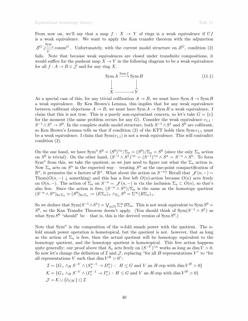
Equivariant homotopy theory Talk 11
From now on, we’ll say that a map f : X → Y of rings is a weak equivalence if Ufis a weak equivalence. We want to apply the Kan transfer theorem with the adjunction
SGSym
// commG
Uoo . Unfortunately, with the current model structure on SG, condition (2)
fails. Note that because weak equivalences are closed under transfinite compositions, itwould suffice for the pushout map X → Y in the following diagram to be a weak equivalencefor all f : A→ B ∈ J and for any ring X.
SymASym f
//
SymB
X // Y
(11.1)
As a special case of this, for any trivial cofibration A → B, we must have SymA → SymBa weak equivalence. By Ken Brown’s Lemma, this implies that for any weak equivalencebetween cofibrant objections A → B, we must have SymA → SymB a weak equivalence. Iclaim that this is not true. This is a purely non-equivariant concern, so let’s take G = efor the moment (the same problem occurs for any G). Consider the weak equivalence e1,1 :S−1 ∧S1 → S0. In the complete stable model structure, both S−1 ∧S1 and S0 are cofibrant,so Ken Brown’s Lemma tells us that if condition (2) of the KTT holds then Sym e1,1 mustbe a weak equivalence. I claim that Sym(e1,1) is not a weak equivalence. This will contradictcondition (2).
On the one hand, we have Symn S0 = (S0)∧n/Σn = (S0)/Σn = S0 (since the only Σn actionon S0 is trivial). On the other hand, (S−1 ∧ S1)∧n = (S−1)∧n ∧ Sn = S−n ∧ Sn. To formSymn from this, we take the quotient, so we just need to figure out what the Σn action is.Now Σn acts on Sn in the expected way – treating Sn as the one-point compactification ofRn, it permutes the n factors of Rn. What about the action on S−n? Recall that J (n,−) =Thom(O(n,−) ↓ something) and this has a free left O(n)-action because O(n) acts freelyon O(n,−). The action of Σn on S−n = J (n,−) is via the inclusion Σn ⊂ O(n), so that’salso free. Since the action is free, (S−n ∧ Sn)/Σn is the same as the homotopy quotient(S−n ∧ Sn)ho Σn ' (S0)ho Σn := (EΣn)+ ∧Σn S
0 = Σ∞(BΣn)+.
So we deduce that Sym(S−1∧S1) =∨n∈N Σ∞+ BΣn. This is not weak equivalent to SymS0 =
S0, so the Kan Transfer Theorem doesn’t apply. (You should think of Sym(S−1 ∧ S1) aswhat SymS0 “should” be – that is, this is the derived version of SymS0.)
Note that Symn is the composition of the n-fold smash power with the quotient. The n-fold smash power operation is homotopical, but the quotient is not. however, that as longas the action of Σn is free, then the actual quotient will be homotopy equivalent to thehomotopy quotient, and the homotopy quotient is homotopical. This free action happensquite generally: our proof above that Sn acts freely on (S−V )∧n works as long as dimV > 0.So now let’s change the definition of I and J , replacing “for all H-representations V ” to “forall representations V such that dimV H > 0”:
I = G+ ∧H S−V ∧ (Sn−1+ → Dn
+) : H ≤ G and V an H-rep with dimV H > 0K = G+ ∧H S−V ∧ (In−1
+ → In+) : H ≤ G and V an H-rep with dimV H > 0J = K ∪ eV,W 2 I
40

Equivariant homotopy theory Talk 11
Requiring dimV > 0 would be sufficient to ensure that Sym condition (2) of the Kan Transfer
Theorem is met, but then ϕH(G+ ∧H S−V ∧ (Sn−1+ → Dn
+)) = S−VH ∧ (Sn−1
+ → Dn+)) and so
if dimV H = 0 then ϕH(f) is not positive cofibrant even though f is. So instead we requirethe mildly stronger condition that dimV H > 0.
Remark 11.2. This modification of the model structure means that the sphere spectrum isno longer cofibrant. This was necessary because e1,1 : S−1 ∧ S1 → S0 is a weak equivalenceand Sym(e1,1) is not a weak equivalence. Condition (2) of the KTT implies (by Ken Brown’sLemma) that Sym takes weak equivalences between cofibrant objects to weak equivalences.Thus, in a model structure where the KTT applies, either S−1 ∧ S1 or S0 must not becofibrant. The positivity condition keeps S−1 ∧ S1 cofibrant and makes S0 not cofibrant.This was more or less necessary, since for any reasonable change of the generating set, wewill have S−n ∧ Sn cofibrant for some n 0, and then the same problem will apply to en,n.
11.2. Bonus: Fibrations are relative Ω-spectra. The category SG is a topologicalmodel category. This means that given i : A → B a cofibration and p : X → Y a fibration,one which must be trivial, there is a contractible choice of lifts A→ X for any diagram:
A //
i
X
p
B // Y
(11.2)
In particular, the lifting condition for a topological model category M is as follows: given(i, p) as above, there is a space of pairs M(A,X) ×M(B, Y ) of maps B → Y and A → X.We want to add the condition that the diagram commutes. There is a continuous mapM(B, Y )→M(A, Y ) given by precomposing with i and a map M(A,X)→M(A, Y ) givenby postcomposing with p. The condition that a pair of maps f : A→ X and g : B → Y makethe diagram commute is that pf = gi. Thus, the space of commuting diagrams is given by
M(A,X)×M(A,Y )M(B, Y ).
Any lift l : B → X gives a commuting diagram by taking f = li and g = pl. Thus there is amap
M(B,X)→M(A,X)×M(A,Y )M(B, Y ).
If M is a topological model category, this map is assumed to be a trivial fibration wheneveri is a cofibration, p a fibration, and one of the two is a weak equivalence.
M(A,X)×M(A,Y )M(B, Y )
M(B,X)triv. fib.
++
p∗
((
i∗
,,
//
M(A,X)
p∗
M(B, Y )i∗
//M(A, Y )
Let’s consider what this means for SG. Consider a map p : X → Y of spectra. It suffices tocheck cofibrancy on the generating trivial cofibrations. We showed above that lifting againstthe maps in K means that p is a levelwise fibration, except that we checked this before weadded the positivity condition. With the extra positivity condition, pV only has to be afibration when dimV H > 0, you can call this a “positive levelwise fibration”. Thus, we
41
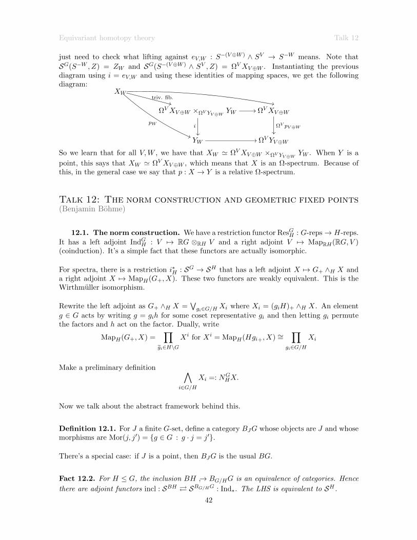
Equivariant homotopy theory Talk 12
just need to check what lifting against eV,W : S−(V⊕W ) ∧ SV → S−W means. Note that
SG(S−W , Z) = ZW and SG(S−(V⊕W ) ∧ SV , Z) = ΩVXV⊕W . Instantiating the previousdiagram using i = eV,W and using these identities of mapping spaces, we get the followingdiagram:
ΩVXV⊕W ×ΩV YV⊕W YW
XWtriv. fib.
++
pW
((
,,
//
i
ΩVXV⊕W
ΩV pV⊕W
YW // ΩV YV⊕W
So we learn that for all V,W , we have that XW ' ΩVXV⊕W ×ΩV YV⊕W YW . When Y is a
point, this says that XW ' ΩVXV⊕W , which means that X is an Ω-spectrum. Because ofthis, in the general case we say that p : X → Y is a relative Ω-spectrum.
Talk 12: The norm construction and geometric fixed points(Benjamin Bohme)
12.1. The norm construction. We have a restriction functor ResGH : G-reps→ H-reps.
It has a left adjoint IndGH : V 7→ RG ⊗RH V and a right adjoint V 7→ MapRH(RG,V )(coinduction). It’s a simple fact that these functors are actually isomorphic.
For spectra, there is a restriction i∗H : SG → SH that has a left adjoint X 7→ G+ ∧H X anda right adjoint X 7→ MapH(G+, X). These two functors are weakly equivalent. This is theWirthmuller isomorphism.
Rewrite the left adjoint as G+ ∧H X =∨gi∈G/H Xi where Xi = (giH)+ ∧H X. An element
g ∈ G acts by writing g = gih for some coset representative gi and then letting gi permutethe factors and h act on the factor. Dually, write
MapH(G+, X) =∏
gi∈H\G
Xi for Xi = MapH(Hgi+, X) ∼=∏
gi∈G/H
Xi
Make a preliminary definition ∧i∈G/H
Xi =: NGHX.
Now we talk about the abstract framework behind this.
Definition 12.1. For J a finite G-set, define a category BJG whose objects are J and whosemorphisms are Mor(j, j′) = g ∈ G : g · j = j′.
There’s a special case: if J is a point, then BJG is the usual BG.
Fact 12.2. For H ≤ G, the inclusion BH → BG/HG is an equivalence of categories. Hence
there are adjoint functors incl : SBH SBG/HG : Ind∗. The LHS is equivalent to SH .
42

Equivariant homotopy theory Talk 12
Definition 12.3. The obvious map G/H → ∗ induces a functor p : BG/H → BG. Define
the norm functor NGH : SH → SG to be the following composite:
SH ' SBH incl→ SBG/HG p⊗→ SBG ' SG.We’re using the fact that there’s an equivalence between genuine H-spectra and spectra withobjectwise H-action (naıve spectra). This is just a statement about categories; they’re notequivalent as homotopical categories.
Properties: NGH commutes with sifted colimits, is symmetric monoidal, and the induced
functor NGH : CommH → CommG is the left adjoint of restriction.
The canonical homotopy presentation is
X ' hocolimV S−V ∧XV .
Then NGHX ' hocolimV S
− IndGH V ∧NGH (XV ), where NG
H (XV ) is an analogously defined normfunctor on spaces with H-action, applied to XV .
Proposition 12.4. (−)∧J : SBJG → SG taking X 7→ ∧j∈J Xj preserves all cofibrations and
acyclic cofibrations between cofibrant objects.
Hence there is a left derived functor (−)∧LJ : hoSBJG → hoSG (it’s the left adjoint in an
adjunction and that descends to an adjunction of homotopy categories).
Corollary 12.5. NGH : CommH CommG : Res is a Quillen adjunction (adjunction on the
level of model categories which descends to the level of homotopy categories where the rightadjoint preserves (co)fibrations, etc.).
Consider
CommH
NGH
//
CommG
SHNGH
// SG
This commutes up to natural isomorphism.
Question 12.6. Is this true on the homotopy level? I.e. does
ho CommH //
NGH
ho CommG
hoSHNGH
// hoSG
Cofibrant commutative rings aren’t cofibrant spectra in general. (The forgetful functor is aright adjoint so it needn’t preserve cofibrancy.)
We have to check:
43

Equivariant homotopy theory Talk 12
• If Rc∼→ R is an approximation in spectra then (Rc)
∧J → R∧J is a weak equivalence.
Proposition 12.7 (HHR B.147). This is true if R is cofibrant in the category of ring spectra.
12.2. Genuine fixed point spectra. Consider the S → SG taking X 7→ X with thetrivial action. This has a right adjoint (−)G : X 7→ (i∗0X)G =: XG (i0 takes it to an ordinaryspectrum, so indexed on Z not representations; levelwise, this still has a G-action, and so youtake the fixed points levelwise). This is the genuine fixed points functor.
Properties:
• π∗(XG) ∼= πG∗ (X) for Ω-G-spectra
• (−)Gf is not compatible with − ∧− and Σ∞(−) (i.e. (Σ∞(X))G 6= Σ∞(XG))
Remark 12.8 (tom Dieck splitting). If K is a G-space, then
((Σ∞K)f )G '∨(H)H≤G
Σ∞(EWGH+ ∧WGH KH)
where WGH = NGH/H is the Weyl group (NG = the normalizer).
12.3. Geometric fixed points. Recall: a G-space EF is universal for a family F if
(EF)H '∗ H ∈ F∅ H /∈ F .
For P the family of all proper subgroups, we get the isotropy separation sequence EP+∧X →X → EP ∧X. This leads to a definition of geometric fixed points.
Definition 12.9. Let ΦG(X) := ((EP ∧X)f )G ∈ S is the geometric fixed point spectrum.
Why do we need another fixed point spectrum? The first one was not compatible with smashproduct and what comes from the level of spaces. But this one is compatible with smashproduct.
Properties:
• ΦG preserves with all weak equivalences
• it commutes with filtered hocolim
• If A ∈ TopG then ΦG(S−V ∧A)∼→ S−V
G ∧AG
• For X ∼ hocolimV S−V ∧ XV then it’s clear from the previous properties that ΦGX '
hocolimS−VG ∧XG
V
• ΦG(X ∧ Y )∼↔ ΦGX ∧ ΦGY (that’s a zigzag of weak equivalences).
Problem 12.10. There’s no natural transformation ΦGX ∧ ΦGY → ΦG(X ∧ Y ).
44

Equivariant homotopy theory Talk 13
The solution is to define the monoidal geometric fixed point functor:
ΦGMX = coeq
( ∨V,W
S−WG ∧JG(V,W )G ∧XG
V ⇒∨V
S−VG ∧XG
V
)
Proposition 12.11. ΦG is the left derived functor of ΦGM i.e. ΦG(X)
∼→ ΦGM (X) for X
cofibrant.
As we’d expect of a functor called the monoidal functor, ΦGM is weakly monoidal, which means
the following. We have an honest natural transformation ΦGMX ∧ΦG
MY → ΦGM (X ∧Y ) which
is a weak equivalence on cofibrant X and Y .
12.4. Relationship between NGH and ΦG
(M).
Proposition 12.12. If H ≤ G is a subgroup, there is a natural transformation ΦHM (−) →
ΦGMN
GH (−) which is an isomorphism (not just a weak equivalence) on cofibrant objects. (Both
are functors from genuine G-spectra to non-equivariant spectra.)
Corollary 12.13. If NGH (Xc)→ NG
H (X) is a weak equivalence for a cofibrant approximation
Xc → X, then there is a chain of weak equivalences ΦHX∼↔ ΦGNG
HX.
Proof. We get a weak equivalence ΦHXc → ΦH(X) (because of property (i) of ΦG).
We’ve seen before that there’s a zigzag of weak equivalences ΦHX∼↔ ΦH
M (Xc)
ΦHXc
∼
oo ∼12.11
// ΦHM (Xc)
∼12.12
// ΦGMN
GH (Xc) oo
∼12.11
// ΦGNGH (Xc)
∼ byassumption
ΦH(X) ΦcNGH (X)
Application 12.14. If H = C2 ≤ C2n ≤ G and X = MUR, then we denote NGHX =
MU ((G)). The corollary we just proved shows that ΦC2nMU ((C2n )) ∼ ΦC2MUR. It followsfrom the (forthcoming) construction of MUR that this is 'MO.
Talk 13: The slice filtration and slice spectral sequence(Koen van Woerden)
13.1. Definitions. We work in G-spectra, and G will be a finite group. Let K ⊂ G be
a subgroup. Let S(m,K) = G+ ∧K SmρK where ρK is the regular representation on K.
Definition 13.1. The set of slice cells is
SC = S(m,K),Σ−1S(m,K) : K ⊂ G,m ∈ Z.
45

Equivariant homotopy theory Talk 13
A slice cell is:
• regular if it is of the form S(m,K)
• induced if it is of the form G+ ∧H SmρH or Σ−1(G+ ∧H SmρH ) for H ( G free if it is induced from H = e
• isotropic if it is induced from e 6= H (but possibly H = G)
Definition 13.2. The dimension of a slice cell is the dimension of the underlying sphere.Let SC≥n be the set of slice cells of dimension ≥ n. Consider the Bousfield localization atthe collection of maps from something in SC≥n to a point. This localization applied to X iscalled Pn. If Y is SC≥n-local, write Y < n, Y ≤ n− 1, or that Y is n-null.
Say that X is slice n-positive, written X > n or X ≥ n + 1, if SG(X,Y ) ' ∗ for all Y suchthat Y ≤ n. Equivalently, X is slice n-positive if PnX ' ∗. The full subcategory of SGgenerated by X > n is called SG>n. Define SG≤n similarly.
There’s a functor called acyclization that takes X to the fiber of X → PnX. Denote this byPn+1X. The PnX are in SG≤n and the Pn+1X are in SG>n, and these are universal with thisproperty.
We have inclusions SC≥n ⊃ SC≥n+1 of sets and hence SG≤n−1 ⊂ SG≤n of categories. This gives
a natural transformation PnX → Pn−1X.
Definition 13.3. The slice tower of X is · · · → PnX → Pn−1X → . . . . PnX is the nth slicesection of X. Take the fiber
PnnXfiber→ PnX → Pn−1X.
PnnX is called the nth slice of X.
Observe that PnnX = PnPnX so it is in SG≥n, but also we have a fiber sequence PnnX →
PnX → Pn−1 where PnX ≤ n and Pn−1X ≤ n− 1, which shows that PnnX ∈ SG≤n.
So the tower looks like...
P 1X
P 11X
oo
P 0X
P 00X
oo
P−1X
P−1−1X
oo
...
46

Equivariant homotopy theory Talk 13
where each PnX
Pnnoo
Pn−1X
is a fiber sequence.
Definition 13.4. The slice spectral sequence is the homotopy spectral sequence of the slicetower:
Es,t1 = πGt−sPttX =⇒ πGt−sX.
The differentials go exactly like the Adams spectral sequence.
Doug: It’s the E2 page if you know that the oddly-indexed slices are zero (e.g. in ourapplication).
Mike: This is the AHSS where you’re cofiltering instead of filtering.
Theorem 13.5. The spectral sequence converges and there are four vanishing lines (marked(i), (ii), (iii), (iv) in the diagram below).
The dotted line has slope |G| − 1. In particular, if you take G = ∗ the spectral sequencedegenerates. (But that doesn’t help because the slices will be Postnikov slices.)
Doug: you could also do a version for H-equivariant homotopy groups; this can be made intoa spectral sequence of bigraded Mackey functors rather than abelian groups. There’s also away to make this RO(G)-graded: take RO(G)-graded homotopy groups, but the index s (thevertical coordinate) is always an integer, as is the index of the slice t, but you can replacethe t in the homotopy group by some other representation other than the trivial one.
Proposition 13.6. Let X be a G-spectrum.
(1) X ≥ 0 iff X is (−1)-connected (“connected” means by mapping in with SV )
(2) X ≥ −1 iff X is (−2)-connected
47

Equivariant homotopy theory Talk 13
(3) X < 0 iff X is 0-coconnected10
(4) X < −1 iff X is (−1)-coconnected
These patterns don’t continue; these dimensions are special.
Proof idea. S0 is a slice cell of dimension 0, S−1 is a slice cell of dimension −1.
Corollary 13.7. P−1 = Pos−1 (where Pos is doing the localization w.r.t. ordinary cells– it’s the equivariant Postnikov filtration) and P−2 = Pos−2. This shows that P−1
−1X =
Σ−1Hπ−1X.
So we can compute P−1−1 .
13.2. Subgroups, induction, and restriction.
Proposition 13.8. Induction and restriction send a slice cell to a (wedge of) slice cells ofthe same dimension.
The norm sends a wedge of regular (i.e. not desuspended) H-cells to a wedge of regularG-cells.
Proposition 13.9. Induction and restriction preserve n-nullness and n-positivity.
Lemma 13.10. Suppose we have a fiber sequence of the form Pn+1 → X → Pn where
Pn+1 > n and Pn ≤ n. Then the canonical maps Pn+1 → Pn+1X and PnX → Pn are weakequivalences.
“If we have a sequence that looks like the right thing then it is the right thing.”
Corollary 13.11. Pn commutes with restriction and induction.
This implies that Pn commutes with restriction and induction, because they determine eachother, and so does Pnn .
Remark 13.12. Taking i∗e shows that the non-equivariant tower underlying the slice tower
is the Postnikov tower.
13.3. More examples.
Proposition 13.13.
(1) X is an (−1)-slice iff there exists a Mackey functor M such that X = Σ−1HM .
10X is n-coconnected if its homotopy groups vanish in dimensions n and above
48

Equivariant homotopy theory Talk 14
(2) X is a 0-slice iff there exists a Mackey functor M with all restrictions injections suchthat X = HM .
Proposition 13.14. X > 0 iff X is (−1)-connected and πu0X = 0.
Proposition 13.15. For n ≥ 0, G/H+ ∧ Sn ≥ n.
For example, when G is the trivial group, the spheres Sn are slice cells of dimension ≥ n,hence in particular Sn ≥ n.
Corollary 13.16. P−1−1 S
−1 = Σ−1HA where A is the Burnside Mackey functor11, and
P 00 S
0 = HZ.
Proof. We already saw the first statement.
For the second statement, taking the P 0 localization is the same as S0 → Pos0 S0 → P 0S0 =P 0 Pos0 S0. (This always happens, not just for S0.) We know that Pos0 S0 = HA andP 0 Pos0 S0 = P 0HA. To compute the zeroth slice, we need to localize down further: takethe fiber of P 0HA → P−1HA to get P 0
0 S0 → P 0HA → P−1HA. But the last term is zero,
so the first map is an equivalence. Write down a fiber sequence HI → HA→ HZ. We havethat HZ ≤ 0 because restriction maps are monos, and HI ≥ 1 by Proposition 13.14. Nowwe conclude by Lemma 13.2 that P 0A = HZ = P 0
0 S0.
13.4. Multiplicative properties. Smashing with SmρG gives an equivalence SG≥n →SG≥n+m|G| because it gives an equivalence between slice cells.
The natural maps SmρG∧PnX → Pn+m|G|(SmρG∧X) and SmρG∧PnX → Pn+m|G|(SmρG∧X)
are weak equivalences.
13.5. Even more examples. For K ⊂ G the m|K|-slice of S(m,K) is HZ ∧ S(m,K),
and the (m|K| − 1)-slice of Σ−1S(m,K) is HA ∧ Σ−1S(m,K).
Proof. G+ ∧ (−) commutes with slice sections can restrict to K = G. Multiplicativityand the previous two examples give the result.
Talk 14: Dugger’s computation for real K-theory (AgnesBeaudry)
Our goal is to compute πC2∗ KR (to be defined later). Let V be a C2-representation, and B a
finite C2-set. Consider Mackey functor homotopy πC2V KR(B) = [SV ∧B+,KR]C2 .
11This is the monoidal unit, and π0S0 = A. Alternatively, it sends H to the (Grothendieck group of) the
Burnside ring of H, and the Burnside ring of H is just finite H-sets.
49

Equivariant homotopy theory Talk 14
The idea is to use this as an example of the slice spectral sequence:
Es,t2 = πt−sPttKR → πt−sKR.
Now let’s talk about Atiyah’s real K-theory. One way to obtain KR is to “kill off stuff fromMUR”. But we’re going to do it more hands on.
The category of “Atiyah–real” vector bundles has objects complex vector bundles p : E → X,for E and X C2–spaces and p a C2–map. Further, we require that the map Ex → Eγ(x) becomplex anti-linear. This means γ(ce) = cγ(e). The morphisms of this category are C2-equivariant maps of vector bundles. This is not the same as C2-complex vector bundlesbecause of the twist we’ve added.
From now on, we assume that G = C2.
Definition 14.1. Let KR(X) be the Grothendieck group of the category of isomorphismclasses of Atiyah–real vector bundles. (We group-complete with respect to direct sum.)
KR : ho TopC2 → Ab is a functor and there’s a corresponding Bott periodicity which
KR(X) ∼= KR(Sρ ∧X+).
(Here, ρ = ρ2 is the regular representation for C2.) We can use this to extend KR to anRO(G)-graded cohomology theory as follows. Recall that any representation can be writtenas n+mσ for n,m ∈ Z. Given any s, t ∈ Z (potentially negative), we let
Ks+tσR (X) := K0
R(Smρ ∧ S−s−tσ ∧X) = K0R(Sm−s+(m−t)σ ∧X) for m 0.
Since K∗R is an RO(G)-graded homology theory, it is represented by a genuine C2-spectrumKR, which is in fact an Ω-C2-spectrum.
Because of Bott periodicity, πC2? KR is determined by πC2
∗ KR for ∗ ∈ Z. (For example,
πC2m+nσKR ∼= πC2
m+nσΣnρKR ∼= πC2m−nKR. In other words, every RO(G)-graded homotopy
group of KR is isomorphic to a Z-graded homotopy group of KR.)
One reason KR is interesting is that it knows about KU (Grothendieck group of isomor-phism classes of complex vector bundles over X ∈ Top) and KO (Grothendieck group ofisomorphism classes of actually real vector bundles over X ∈ Top).
Claim 14.2. If XC2 = X then KR(X) ∼= KO(X).
Proof. The categories of actually real and Atiyah real vector bundles on X are equiv-alent. Here is a sketch of why. Given E → X an actually real vector bundle, letting the C2
action on C⊗RE be the one coming from complex conjugation on C gives C⊗RE the structureof Atiyah-real vector bundle. Given an Atiyah-real bundle, we can take fixed points to obtainan actually real vector bundle EC2 → XC2 = X. Since it is an equivalence of categories, theGrothendieck completions are the same.
50

Equivariant homotopy theory Talk 14
In particular, KR(∗) = KO(∗). So π∗KR(C2/C2) ∼= π∗KO. Atiyah’s KR also know aboutKU . Here is how.
Claim 14.3. KR(X × C2) ∼= KU(X)
There is no ambiguity about X × C2 as a C2-space: The action coming from the diagonalaction and the one coming from the trivial action on X give isomorphic spaces.
Proof. Again, this comes from an equivalence of categories between complex vectorbundles on X and Atiyah-real bundles on C2 × X. Given an Atiyah–real bundle E → X,consider the pull-back
E
i∗eE
oo
X X × e? _oo
The right bundle is a complex vector bundle. Further, given a complex vector bundle E → X,let E → X be the conjugate bundle. Then E t E → X × C2 = Xe t Xγ is an Atiyah-realvector bundle on X × C2.
Corollary 14.4. π∗KR(C2/e) ∼= π∗KU
Mike talked about the fact that ΩhC8O ' ΩC8
O ; this is the fixed point theorem. K-theory also
has a fixed point theorem KC2R∼= KhC2
R .
Recall the isotropy separation sequence
EP+ → S0 → EPwhere P is the family of proper subgroups of G. We have
EPH =
∗ H ( G
∅ H = G
EPH =
∗ H ( G
S0 H = G
It follows that, for G = C2, EP is a model for EC2 since the only proper subgroup of C2 isthe trivial subgroup. Also, we can write EC2 = colimn→∞ S(n∞) = S(∞σ), where S(nσ) is
the unit sphere with antipodal action. Then EC2 = colimn→∞ Snσ = S∞σ, and S∞σ has 2
fixed points, ∞ and 0.
Mingcong will show in his lecture that if X is an equivariant homotopy ring spectrum and
EG ∧ X is contractible, then X → XEG+ is a weak equivalence. This implies that XG →(XEG+)G = XhG is equivalence.
Claim 14.5. EC2 ∧KR ' ∗
51
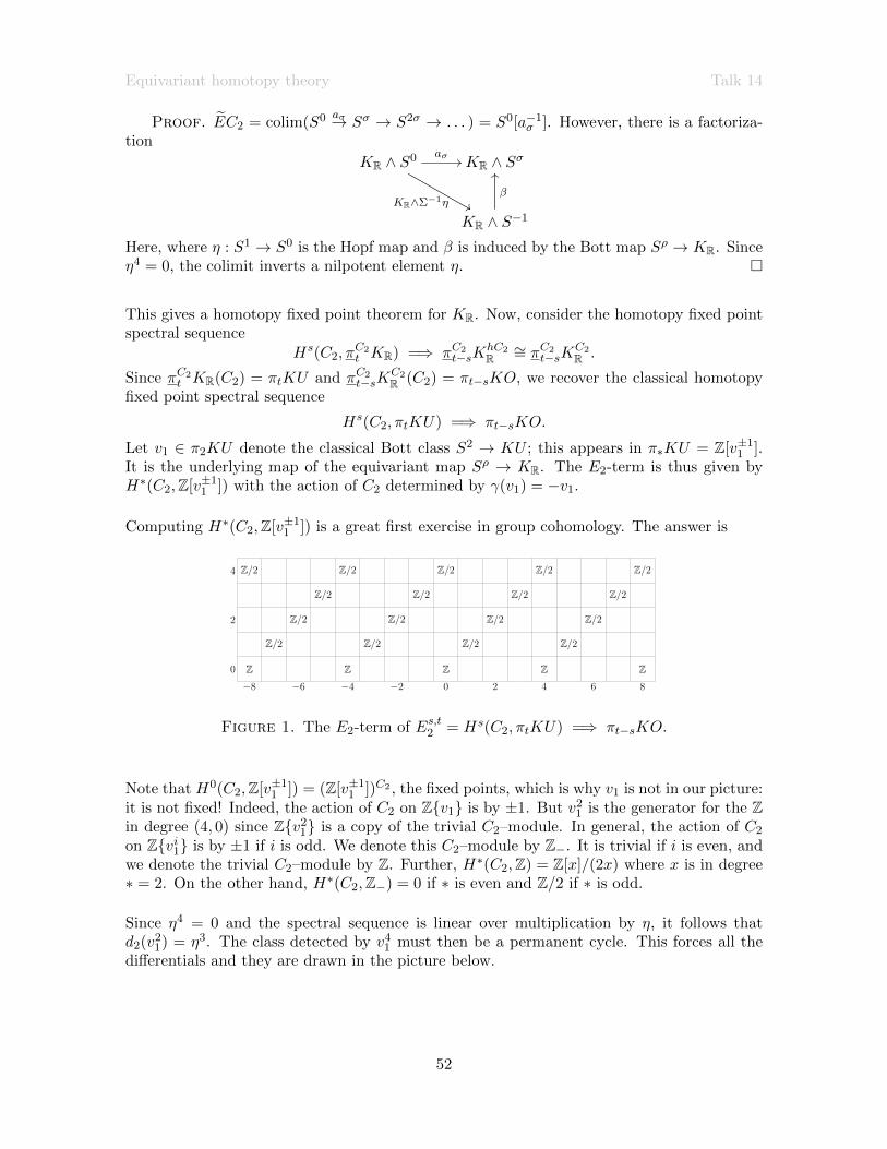
Equivariant homotopy theory Talk 14
Proof. EC2 = colim(S0 aσ→ Sσ → S2σ → . . . ) = S0[a−1σ ]. However, there is a factoriza-
tion
KR ∧ S0 aσ //
KR∧Σ−1η &&
KR ∧ Sσ
KR ∧ S−1
β
OO
Here, where η : S1 → S0 is the Hopf map and β is induced by the Bott map Sρ → KR. Sinceη4 = 0, the colimit inverts a nilpotent element η.
This gives a homotopy fixed point theorem for KR. Now, consider the homotopy fixed pointspectral sequence
Hs(C2, πC2t KR) =⇒ πC2
t−sKhC2R∼= πC2
t−sKC2R .
Since πC2t KR(C2) = πtKU and πC2
t−sKC2R (C2) = πt−sKO, we recover the classical homotopy
fixed point spectral sequence
Hs(C2, πtKU) =⇒ πt−sKO.
Let v1 ∈ π2KU denote the classical Bott class S2 → KU ; this appears in π∗KU = Z[v±11 ].
It is the underlying map of the equivariant map Sρ → KR. The E2-term is thus given byH∗(C2,Z[v±1
1 ]) with the action of C2 determined by γ(v1) = −v1.
Computing H∗(C2,Z[v±11 ]) is a great first exercise in group cohomology. The answer is
8 6 4 2 0 2 4 6 8
0
2
4
Z
Z/2
Z/2
Z/2
Z/2Z/2
Z
Z/2
Z/2
Z/2
Z/2
Z
Z/2
Z/2
Z/2
Z/2
Z
Z/2
Z/2
Z/2
Z/2
Z
1Figure 1. The E2-term of Es,t2 = Hs(C2, πtKU) =⇒ πt−sKO.
Note that H0(C2,Z[v±11 ]) = (Z[v±1
1 ])C2 , the fixed points, which is why v1 is not in our picture:it is not fixed! Indeed, the action of C2 on Zv1 is by ±1. But v2
1 is the generator for the Zin degree (4, 0) since Zv2
1 is a copy of the trivial C2–module. In general, the action of C2
on Zvi1 is by ±1 if i is odd. We denote this C2–module by Z−. It is trivial if i is even, andwe denote the trivial C2–module by Z. Further, H∗(C2,Z) = Z[x]/(2x) where x is in degree∗ = 2. On the other hand, H∗(C2,Z−) = 0 if ∗ is even and Z/2 if ∗ is odd.
Since η4 = 0 and the spectral sequence is linear over multiplication by η, it follows thatd2(v2
1) = η3. The class detected by v41 must then be a permanent cycle. This forces all the
differentials and they are drawn in the picture below.
52

Equivariant homotopy theory Talk 14
8 6 4 2 0 2 4 6 8
0
2
4
Z
Z/2
Z/2
Z/2
Z/2Z/2
Z
Z/2
Z/2
Z/2
Z/2
Z
Z/2
Z/2
Z/2
Z/2
Z
Z/2
Z/2
Z/2
Z/2
Z
1Figure 2. The differentials in Es,t2 = Hs(C2, πtKU) =⇒ πt−sKO.
The conclusion is that π∗KO = Z[b±1, η, w]/(2η, η3, w2 = 4b) ∼= πC2∗ KR(pt). The E∞–term is
drawn below.
8 6 4 2 0 2 4 6 8
0
2
Z
Z/2
Z/2
Z Z
Z/2
Z/2
Z Z
1
Figure 3. The E∞-term of the spectral sequence Es,t2 = Hs(C2, πtKU) =⇒ πt−sKO.
14.1. Slice spectral sequence. We return to our goal of computing
Es,t2 = πC2t−sP
ttKR(C2/H) =⇒ πC2
t−sKR(C2/H) =
πt−sKO H = C2
πt−sKU H = e
We need to know the slices. Koen told us that P−1−1KR ' Σ−1Hπ−1KR. However,
π−1KR(C2/H) =
π−1KO H = C2
π−1KU H = e
Since π−1KO = π−1KU = 0, this is the zero Mackey functor. Therefore, P−1−1KR ' ∗.
Here is a result which you can find in Mike’s “The equivariant slice filtration: A primer”.
Theorem 14.6. If π0X has all restrictions monomorphisms, then P 00X = Hπ0X.
You can check that π0KR = Z, the constant Mackey functor, which has all restrictionsidentities by definition. Therefore, P 0
0KR = HZ.
Now, recall that we can suspend by regular representations ρ and shift the slices around.However, ΣρKR ' KR by Bott periodicity. So knowing the −1 and 0 slices gives us all of theslices. We get the following result:
53
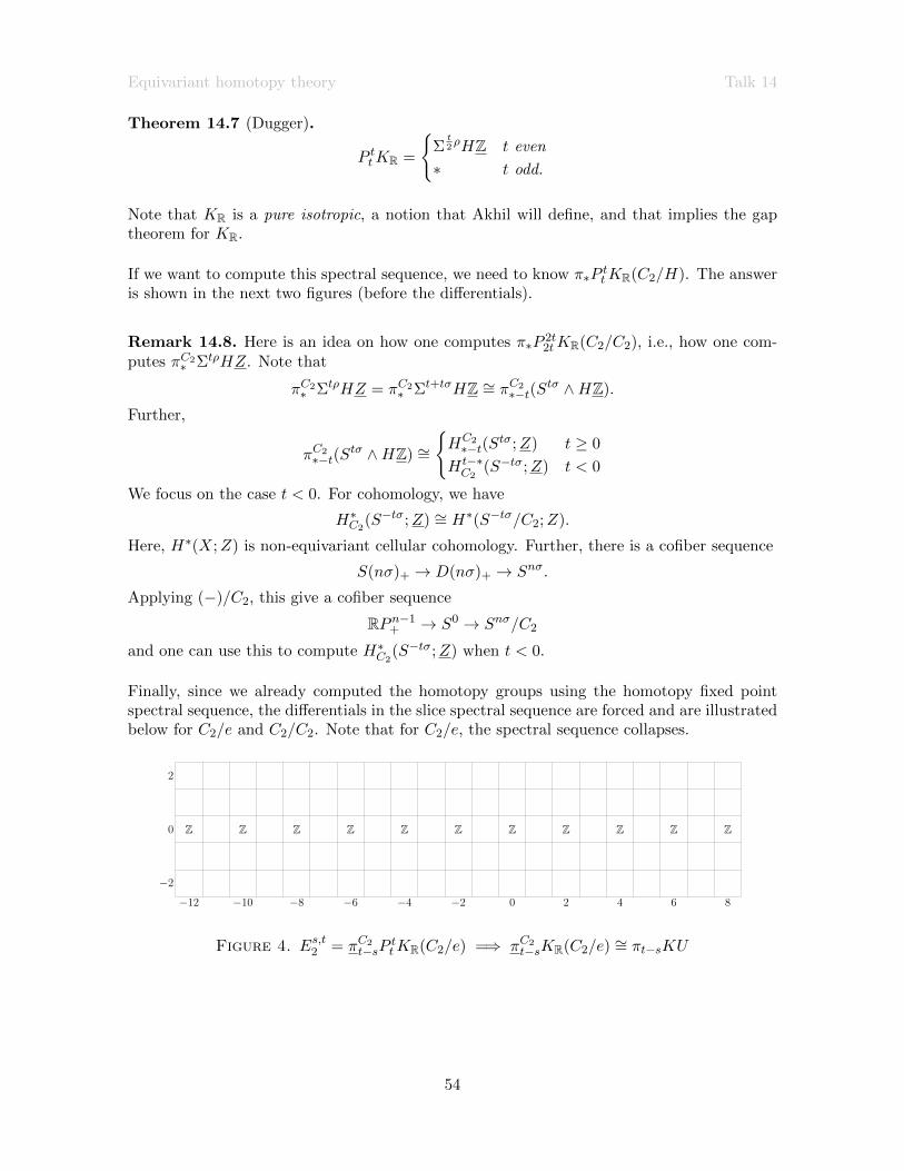
Equivariant homotopy theory Talk 14
Theorem 14.7 (Dugger).
P ttKR =
Σt2ρHZ t even
∗ t odd.
Note that KR is a pure isotropic, a notion that Akhil will define, and that implies the gaptheorem for KR.
If we want to compute this spectral sequence, we need to know π∗PttKR(C2/H). The answer
is shown in the next two figures (before the differentials).
Remark 14.8. Here is an idea on how one computes π∗P2t2tKR(C2/C2), i.e., how one com-
putes πC2∗ ΣtρHZ. Note that
πC2∗ ΣtρHZ = πC2
∗ Σt+tσHZ ∼= πC2∗−t(S
tσ ∧HZ).
Further,
πC2∗−t(S
tσ ∧HZ) ∼=HC2∗−t(S
tσ;Z) t ≥ 0
Ht−∗C2
(S−tσ;Z) t < 0
We focus on the case t < 0. For cohomology, we have
H∗C2(S−tσ;Z) ∼= H∗(S−tσ/C2;Z).
Here, H∗(X;Z) is non-equivariant cellular cohomology. Further, there is a cofiber sequence
S(nσ)+ → D(nσ)+ → Snσ.
Applying (−)/C2, this give a cofiber sequence
RPn−1+ → S0 → Snσ/C2
and one can use this to compute H∗C2(S−tσ;Z) when t < 0.
Finally, since we already computed the homotopy groups using the homotopy fixed pointspectral sequence, the differentials in the slice spectral sequence are forced and are illustratedbelow for C2/e and C2/C2. Note that for C2/e, the spectral sequence collapses.
12 10 8 6 4 2 0 2 4 6 8
2
0
2
Z Z Z Z Z Z Z Z Z Z Z
1Figure 4. Es,t2 = πC2t−sP
ttKR(C2/e) =⇒ πC2
t−sKR(C2/e) ∼= πt−sKU
54

Equivariant homotopy theory Talk 15
12 10 8 6 4 2 0 2 4 6 8
4
2
0
2
4
Z Z/2
Z/2
Z/2
Z Z/2
Z/2
Z/2
Z/2
Z/2
Z Z
Z/2
Z/2
Z/2
Z/2
Z
Z/2
Z/2
Z/2
Z/2
Z
1
Figure 5. Es,t2 = πC2t−sP
ttKR(C2/C2) =⇒ πC2
t−sKR(C2/C2) ∼= πt−sKO.
This can all be packaged using Mackey functors. We use the following notation for therelevant C2–Mackey functors:
Symbol • •
Lewis Diagram Z1
Z
2
VV 0
Z−
VV Z/2
0
TTZ
2
Z
1
VV Z/2
0
Z−
1
TT
Then the slice spectral sequence for KR is described in the following nice picture.
12 10 8 6 4 2 0 2 4 6 8
4
2
0
2
4
•
•
1
Figure 6. The slice spectral sequence Es,t2 = πC2t−sP
ttKR =⇒ πC2
t−sKR. Thedashed line in the first quadrant is an exotic transfer and the dotted line inthe third quadrant an exotic restriction.
55
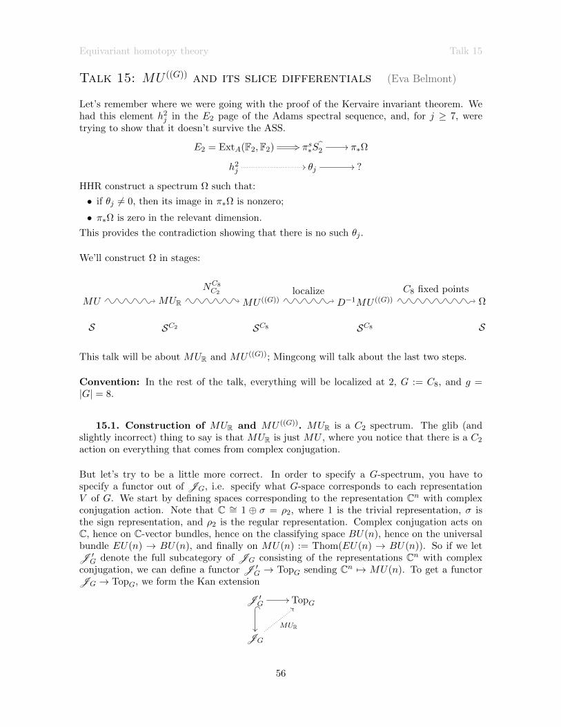
Equivariant homotopy theory Talk 15
Talk 15: MU ((G)) and its slice differentials (Eva Belmont)
Let’s remember where we were going with the proof of the Kervaire invariant theorem. Wehad this element h2
j in the E2 page of the Adams spectral sequence, and, for j ≥ 7, weretrying to show that it doesn’t survive the ASS.
E2 = ExtA(F2,F2) +3 πs∗S2// π∗Ω
h2j
// θj // ?
HHR construct a spectrum Ω such that:
• if θj 6= 0, then its image in π∗Ω is nonzero;
• π∗Ω is zero in the relevant dimension.
This provides the contradiction showing that there is no such θj .
We’ll construct Ω in stages:
MU MUR MU ((G)) D−1MU ((G)) Ω
S SC2 SC8 SC8 S
NC8C2 localize C8 fixed points
This talk will be about MUR and MU ((G)); Mingcong will talk about the last two steps.
Convention: In the rest of the talk, everything will be localized at 2, G := C8, and g =|G| = 8.
15.1. Construction of MUR and MU ((G)). MUR is a C2 spectrum. The glib (andslightly incorrect) thing to say is that MUR is just MU , where you notice that there is a C2
action on everything that comes from complex conjugation.
But let’s try to be a little more correct. In order to specify a G-spectrum, you have tospecify a functor out of JG, i.e. specify what G-space corresponds to each representationV of G. We start by defining spaces corresponding to the representation Cn with complexconjugation action. Note that C ∼= 1 ⊕ σ = ρ2, where 1 is the trivial representation, σ isthe sign representation, and ρ2 is the regular representation. Complex conjugation acts onC, hence on C-vector bundles, hence on the classifying space BU(n), hence on the universalbundle EU(n) → BU(n), and finally on MU(n) := Thom(EU(n) → BU(n)). So if we letJ ′
G denote the full subcategory of JG consisting of the representations Cn with complexconjugation, we can define a functor J ′
G → TopG sending Cn 7→ MU(n). To get a functorJG → TopG, we form the Kan extension
J ′G _
// TopG
JG
MUR
<<
56

Equivariant homotopy theory Talk 15
(Actually, I just lied a little bit: you’re supposed to do a cofibrant replacement on the functorJ ′
G → TopG before Kan extending. See HHR §B.12.7.) This has some nice properties:
• MUR is a commutative ring G-spectrum;
• the underlying (nonequivariant) spectrum of MUR is just MU ;
• ΦC2MUR 'MO.
The second point is a consequence of the canonical homotopy presentation
MUR∼← holimS−nρ2 ∧MU(n).
15.2. Some elements in π∗MU ((G)).
Theorem 15.1. There are some elements ri ∈ πu2iMU ((G)) such that:
• they “generate”, in the sense that πu∗MU ((G)) ∼= Z2[γjri] i≥00≤j<4
where γ ∈ G/C2 (so the
G/C2-translates of the ri’s are generators);
• they have good fixed-point properties (to be described later).
It turns out that you can upgrade these non-equivariant homotopy classes to C2-equivarianthomotopy classes:
Theorem 15.2. We have an isomorphism⊕j≥0
πu2jMU ((G)) ∼=⊕j≥0
πC22ρ2i∗C2
MU ((G))
and moreover⊕j≥0
πu2j∧m
MU ((G)) ∼=⊕j≥0
πC22ρ2i∗C2
∧m
MU ((G)) for any m ≥ 1.
Since i∗C2MU ((G)) ∼= MU∧4
R as C2-spectra, we now have classes in πC22ρ2i∗MU ((G)); let ri denote
the C2-equivariant homotopy class corresponding to ri under the above isomorphism.
Just asMU ((G)) was obtained fromMUR from taking the norm, we can produceG-equivarianthomotopy classes Nri ∈ πGiρGMU ((G)) as well by taking the norm:
[Siρ2 , i∗C2MU ((G))]
NGC2−→ [NG
C2Siρ2 , NG
C2i∗C2
MU ((G)]
∼= [SIndGC2iρ2 , NG
C2i∗C2
MU ((G))]
∼= [SiρG , NGC2i∗C2
MU ((G))]
counit−→ [SiρG ,MU ((G))]
where the last map is the counit of the adjunction between restriction i∗C2and norm that
happens in CommG. This is sometimes called the internal norm.
Recall that π∗ΦGMU ((G)) ∼= π∗MO = Z/2[hi : i 6= 2k − 1]. It turns out that ΦGNri = hi
(and ΦGNri when i = 2k − 1 for some k). This is what I meant earlier when I said the rihad “good fixed point properties”.
57

Equivariant homotopy theory Talk 15
15.3. Slice spectral sequence review and slice theorem preview. Recall the slicetower for a G-spectrum X looks like
...
P 1X
P 11X
fiberoo
X //
==
FF
P 0X
P 00X
fiberoo
...
where PnnX → PnX → Pn−1X are fiber sequences and PnX is made out of slice cells ofdimension ≤ n.
Before, we talked about the spectral sequence obtained by taking integer-graded homotopy ofthis tower; now, we’re going to take RO(G)-graded homotopy of the slice tower. The resultis a spectral sequence
Es,V2 = πGV−sPdimVdimV X =⇒ πGV−sX,
where the differentials have the form dr : Es,V2 → Es+r,V+(r−1)2 . Fortunately, we will only be
considering the piece of this with V = ∗− 2kσ where ∗ ∈ Z and k is fixed; the resulting thingis now doubly-integer-graded, and the differentials stay in this piece.
We want to apply this to X = MU ((G)).
In general, computing PnnX is hard. But,∨n
Pnn
(∨slice cells
)' HZ ∧ (those slice cells).
MU ((G)) isn’t a wedge of slice cells, but the slice theorem, which we’ll hear more about inAkhil’s talk, says that it’s the next best thing:
Theorem 15.3 (Slice theorem). There is a map∨slice cells→MU ((G))
that is an equivalence after applying Pnn (−). In particular, this wedge of slice cells can bewritten S0[G · ri]i≥0 (notation explained below). So, there is an equivalence
HZ ∧ S0[G · ri] ∼→∨n≥0
PnnMU ((G)).
About the notation: first let S0[SV ] :=∨n≥0(SV )∧n be the free associative algebra on SV
(the notation should remind you of a polynomial algebra). If x is the class of the canonicalbottom map SV → S0[SV ], then we also write S0[x] := S0[SV ]. That’s a polynomial ring inone variable. Our wedge of slice cells S0[G · ri] := S0[γj · ri] i≥0
0≤j<4should be thought of as
58

Equivariant homotopy theory Talk 15
a polynomial ring in infinitely many variables, one for each G/C2-translate of ri. (Here γ isagain the generator of G/C2.)
15.4. Elements in E2. Now we are ready to describe elements in the E2 page of theslice spectral sequence for MU ((G)). Recall we’re restricting to V of the form i+jσ for i, j ∈ Z(we’ll restrict to ∗−2kσ for fixed k later). So we’re looking for maps S∗+∗σ → ∨
PnnMU ((G)),and by the slice theorem it’s clear that we should be looking for maps S∗+∗σ → HZ∧S0[G·ri].
There are three classes of elements we’re going to talk about; the first two are gotten bymapping into HZ and the third is gotten by mapping into S0[G · ri].• aV is the Hurewicz image of S0 → SV . (This is the Euler class of V .) In this talk,
we’ll only care about a := aσ ∈ π−σHZ, which is in E1,1−σ2 = π−σP
00MU ((G)). It is a
permanent cycle.
• For any oriented representation12 V , I claim that the restriction map
HGV (SV ;Z)→ Hu
|V |(SV ;Z)
is an isomorphism. In particular, 2× any representation is an orientable representation.So define u := u2σ ∈ HG
2σ(S2σ;Z) to be the class corresponding to the orientation class
in Hu2 (S2σ;Z). This is in E0,2−2σ
2 = π2−2σP00MU ((G)).
• Recall Nri is a homotopy class given by a map SiρG → S0[γjri] → MU ((G)). To get it
into the right degree, we consider fi : SiaρG→ SiρG → S0[G · ri]→ HZ ∧ S0[G · ri]. This
is in E(g−1)i,gi2 = πiP
gigiMU ((G)) and it is a permanent cycle (this is just a suspension of
Nri, which was an actual G-equivariant homotopy class).
Here’s a picture of where these elements sit in the E2 term. Soon I’ll discuss some propertiesof this picture.
The vanishing line comes from the vanishing line on the slice spectral sequence that Koentalked about, but it’s a little different because we’ve got the piece of the spectral sequencewhere V = ∗− 2kσ for ∗ ∈ Z (Koen only discussed the case where both indices are integers).
12An orthogonal representation G→ O(N) is oriented if it factors through SO(n); or equivalently, if there is
an element in∧|V | V fixed by G; or equivalently, if there is an element (an orientation class) in HG(SV ;Z).
59
Equivariant homotopy theory Talk 15
15.5. A differential in the slice spectral sequence for MU ((G)).
Theorem 15.4. There is a differential d1+(2k−1)gu2k−1
= a2kf2k−1, and all previous differ-
entials on u2k−1are zero.
Proof. Note: this proof is not quite the same as the one in the HHR paper; I learnedthis from Po Hu’s MSRI talk.
Here are the main steps of the proof:
(1) Show we’ve described everything in the colored region.
(2) a−1π∗X ∼= π∗ΦGX. In particular, a−1π∗MU ((G)) ∼= π∗Φ
GMU ((G)) ∼= π∗MO ∼= Z/2[hi :i 6= 2j − 1 for some j].
(3) a?f2k−1 needs to be hit by a differential (for some value of ?).
(4) It has to be a2kf2k−1.
(5) And it has to be killed by the advertised differential.
I’m not going to talk about (1) because it’s not the interesting part; this corresponds to mostof §9.1 in the paper before the proof of 9.9. The point is to show that induced slice cells don’tcontribute in this region, and then explicitly analyze the non-induced slice cells.
(2) is Lemma 15.5. (3) follows from this.
(4) I’m not going to talk about this either – you assume some anf2k−1 were hit by a longerdifferential and get a contradiction because the degree of the source of the differential doesn’tmake sense.
(5) Use induction on k. The claim is that everything in the known region except the twogreen lines in the diagram is zero on our stage of the induction – this is because all of theelements in the middle (see hypothetical green dot in the picture) are a product of somepermanent cycles (a’s and fi’s) and u raised to a power < 2k−1. Even though we’ve only
shown that u2i for i < k − 1 support differentials, we’ve also shown that dr(u2i) = 0 for r <
the differential that is actually nonzero. So e.g. if we have u6 = u2u4, and if dj(u2) 6= 0,
we have d(u2u4) = d(u2)u4 6= 0. So our hypothetical green dot (and everything else in the
middle) is gone at this stage of the induction. We’ve already claimed that a2kf2k−1 has to gethit, and it has to get hit at this stage because there are no more opportunities afterwards.
60

Equivariant homotopy theory Talk 16
Lemma 15.5. π∗ΦGX ' a−1π∗X
Proof. It has been shown in previous talks that a−1πG∗ X = colim(πG∗ Xa→ πG∗ X
a→ . . . )is just smashing X with Sσ a bunch of times. On the other hand, we’ve also shown that
π∗(EP ∧ X)G = πG∗ ((limn→∞ Snσ) ∧ X). (I guess I’m ignoring fibrant replacement. . . the
claim is that it doesn’t matter.)
For the record, I’ll actually tell you some facts about degree:
aσ ∈ E1,1−σ2 = π−σP
00MU ((G))
fi ∈ E(g−1)i,gi2 = πiP
gigiMU ((G))
u = u2σ ∈ E0,2−2σ2 = π2−2σP
00MU ((G))
where g = |G| = 7.
Talk 16: The reduction, gap, and slice theorems (AkhilMathew)
ConsiderMU ((G8)) = NC8C2
(MUR) from last time. There’s going to be a classD ∈ π19ρ8MU ((C8))
that Mingcong will talk about. Then they define ΩO = (MU ((C8)))[D−1]. Then we’re going
to construct a non-equivariant spectrum Ω := ΩC8O and that is ∼= ΩhC8
O by the homotopy fixed
point theorem (the O stands for octonions).
One of the key theorems is
Theorem 16.1 (Gap theorem). πiΩ = 0 for −4 < i < 0
Ω is 256-periodic, so this is going to imply that the Kervaire classes go to 0 if they existed.
61

Equivariant homotopy theory Talk 16
We have
ΩO ' hocolim(MU ((C8)) D→ Σ−19ρ8MU ((C8)) → . . . ) (16.1)
HHR proved that the gap is visible at each stage. In fact, πC8i (Σnρ8MU ((C8))) = 0 for
−4 < i < 0 and all n. They proved this by showing that this gap is true for a large class ofG-spectra. This is proved using the slice spectral sequence.
We cared about a non-equivariant spectrum Ω, but the important thing is to pass through aC8-spectrum and consider its non-homotopy-fixed points.
I’m going to review a definition from Koen’s talk. Throughout, G will be a cyclic 2-group.
Definition 16.2. A slice in SG is a pure cellular spectrum if it is a wedge of HZ∧ S(m,K)
where S(m,K) = G+ ∧K SmρK for K ⊂ G.
Definition 16.3. AG-spectrumX is pure and isotropic if all the slices PnnX are pure cellular,
i.e. wedges of HZ ∧ S(m,K) where m|K| = n and where K 6= 1.
In particular, these are all even slices, so this is saying that all the odd-dimensional slicesvanish.
There are two theorems that will imply the gap theorem.
Theorem 16.4 (Slice Theorem). MU ((G)) = NGC2
(MUR) is pure and isotropic.
Theorem 16.5 ((General) gap theorem). If X ∈ SG is pure and isotropic and G 6= 1, thenπGi X = 0 for −4 < i < 0.
Remark 16.6. If X is pure and isotropic, so is SmρG ∧X; smashing with a regular repre-sentation sphere just shifts the slice filtration.
So if we know that MU ((C8)) is pure and isotropic, then so are all the other terms in thehocolim in (16.1). (Note that the homotopy colimit of pure and isotropic things needn’t bepure and isotropic, but it works in this case, because these maps are inclusion of a wedgesummand.)
Example 16.7. As Agnes explained, KR ∈ SC2 has slices of the form HZ ∧ Snρ2 . We cansee the gap in the homotopy: πC2
i KR ∼= πiKO = 0 if −4 < i < 0.
You can try to run this story with p-groups, and still get a gap −4 < i < 0.
If X is pure and isotropic, we know that X ' lim←−PnX and the fiber of PnX → Pn−1X looks
like a wedge of summands of the form HZ∧ S(m,K) where m|K| = n and K 6= 1. By usingthis tower, it suffices to show that you have the gaps on each of these fibers, because then youcan use a LES. It is enough to show that πGi (HZ∧(G+∧KSmρK )) = 0 in the range. Induction
62

Equivariant homotopy theory Talk 16
and coinduction are the same for G-spectra; by the adjunction this is ∼= πKi (HZ∧ SmρK ). Itsuffices to prove:
Lemma 16.8 (Cell Lemma). If G 6= 1 is a cyclic 2-group, then πGi HZ ∧ SkρG = 0 for−4 < i < 0.
Aside from one edge case, G can be any finite group. It suffices to make a calculation ofBredon homology.
Proof. We only describe the proof for i = −1 and −2, because those are all that isneeded for the Kervaire result.
This is [Si, HZ ∧ SkρG ] ' [ΣiS−kρG , HZ]. We need a general observation about Bredonhomology with coefficients in the constant Mackey functor: if X is a G-CW complex,
[Σ−jX,HZ]SG ' Hj(X/G;Z). (Why? Check on orbits, and then use the cell decompo-sition. Warning: this doesn’t work in homology.)
Consider maps [ΣiS−kρG ;HZ]G. This vanishes for k ≥ 0: it is ∼= [S0, HZ ∧ S−i ∧ SkρG ]. Ifk ≥ 0, the RHS is 0-connected (also remember we’re considering −4 < i < 0), which meansthere are no maps from S0 into it. So it suffices to consider the case when k < 0.
So take k = −` ofr ` > 0. We’re considering [ΣiS`ρG ;HZ]G ∼= H−i(S`ρG/G;Z). I need toshow that this is zero for i = −1,−2 (for the general gap theorem, you also need −3, but forthe part needed for the Kervaire theorem you only need these i’s). If ` ≥ 2, S`ρG is a 2-fold
suspension Σ2S(`ρG−2). We’re using the fact that if you have a connected space and take it’sorbits, it’s still connected, and also that orbits commute with suspension. So you’re taking
H−i of the 2-fold suspension of a connected space S`ρG−2/G. So i = −1 is OK.
It suffices to consider ` = 1, i = −2. Write ρG = 1 ⊕ ρG, so H2(SρG/G;Z) = 0 iffH1(SρG/G;Z) = 0. There is a cofiber sequence S(ρG)+ → S0 → SρG called the Eu-ler sequence. Quotienting by the action of G, you have S(ρG)+/G → S0 → SρG/G. SoSρG/G = Σ(S(ρG)/G) which is the suspension of a connected space and hence it has no H1.(To do i = −3, you have to push the calculation one step further.)
We’re trying to understand the slice tower of MU ((G)). We’re going to build PnMU ((G))
by “algebraic methods”; then you have to prove that the thing you’ve produced is the slicetower. We start with a toy case.
Example 16.9. Let R be a ring spectrum with π∗R = Z[x] for |x| = 2. R/x is defined to
be the cofiber of Σ2Rx→ R, and in our case that is ' HZ. Similarly, R/xn ' cofib(Σ2nR
xn→R) ' τ≤2n−2R. I claim that the sequence R/xn is the Postnikov tower.
Example 16.10. Let R be an E∞ ring spectrum, where π∗R = Z[x, y] where |x| = 2, |y| = 4.Again we’re going to try to construct the Postnikov tower. Now it’s not sufficient to modout by powers of x and y alone; you need to mod out by powers of the augmentation ideal.Define A1 = S0[S2] =
∨i≥0 S
2i. There’s a natural map A1 → R of associative rings that
63
Equivariant homotopy theory Talk 16
sends S2 7→ x. Let A2 = S0[S4] =∨j≥0 S
4j ; there’s a map A2 → R sending S4 7→ y. Get
a map A1 ∧ A2 → R ∧ R → R, where A1 ∧ A2 '∨i,j≥0 S
2i+4j . Its homotopy looks like thehomotopy groups of spheres where you’ve added an extra class in degree 2 and in degree 4.Here we use that R is commutative. If R is associative, you have a map R ∧R→ R but it’sonly a map of rings if R is commutative.
I’m going to define an ideal (sub-wedge) in this ring spectrum of classes that have degree≥ 2n: define I2n =
∨i,j
2i+4j≥2nS2i+4j ⊂ A. This is an (A,A)-bimodule. So I can form a tower
A/I2n, and its associated graded I2n/I2n+2 '∨
i,j2i+4j=2n
., an (A,A)-bimodule whose action
is coming from A→ S0 (the classes S2 and S4 aren’t doing anything because they push youinto higher filtration).
How to construct the Postnikov tower of R? Using the augmentation ideal, form R ∧A S0,and the claim is that that is ' HZ. More generally, R ∧A (A/I2n) ' τ≤2n−2R.
(These are monoid rings, but not twisted yet.)
HHR try to do this equivariantly.
Theorem 16.11. πu∗MU ((G)) = Z[G · r1, G · r2, . . . ] where G · ri = ri, γri, . . . , γ|G|/2−1riwhere γ ∈ G is a generator, and γ|G|/2ri = (−1)iri.
Each ri refines Siρ2ri→ i∗C2
MU ((G)).
For each i, define S0[Siρ2 ] ' ∨j≥0 Sijρ2 to be the free associative algebra, and define S0[G ·
ri] = NGC2
(S0[Siρ2 ]). Norming from a polynomial ring on one generator gets you a polynomialring on a bunch of generators that are permuted by the group.
The observation is that for each i, I get a map S0[G · ri] → MU ((G)) which does what
you think it does on πu∗ . Why? ri is a map S0[Siρ2 ] → i∗C2MU ((G)), and so you can form
S0[G·ri] ' NGC2
(S0[Siρ2 ])→ NGC2
(i∗C2MU ((G)))→MU ((G)); we’re using the fact that MU ((G))
is commutative and the last map is the counit map.
Form S0[G · ri] =∧i S
0[G · ri] → MU ((G)); this is ' A and is called a “refinement ofhomotopy”.
Theorem 16.12 (Reduction theorem). MU ((G)) ∧A S0 ' HZ.
This is due to HHR in general, but for C2 it is due to Hu-Kriz. There’s an analogue of this ismotivic homotopy theory, where it is due to Hopkins-Morel, separately published by Hoyois.
Now more about the slice theorem. We had
A = S0[G · ri]i≥0 =∨
f :J→Z≥0finitely supported
Sρf
where64
Equivariant homotopy theory Talk 17
• J =⊔i>0G/C2
• Kf = stab(f)
• ρf is the multiple of the regular representation of Kf of dimension 2∑
j∈J if(j)
Let I2n ⊂ A be all representation spheres of dimension ≥ 2n. This is a sub-bimodule of A.You don’t need to use G-spectra; this is happening at the level of ordinary spectra. TheI2n will form a descending filtration of A, and I2n/I2n−2 is a wedge of isotropic slice cells ofdimension 2n acted on through the augmentation.
I claim that MU ((G))∧A(A/I2n) ' P 2n−2MU ((G)). The proof is similar to the non-equivariant
case. The associated graded is MU ((G)) ∧A (I2n/I2n+2). Because this is acted on by the
augmentation ideal, this is the same as (MU ((G)) ∧A S0) ∧ I2n/I2n+2. This is the same asHZ∧ (pure and isotropic slice cells). So each of the terms in the associated graded is madeout of slice cells. There’s a recognition theorem that tells you this is actually the slice tower.
For the reduction theorem, you’re trying to prove that MU ((G)) ∧A S0 ' HZ. For G = 1,this is due to Quillen and Milnor. In general, this is proved along with the slice theorem.Prove the reduction theorem for C2n , use that to prove the slice theorem for C2n , use that toprove the reduction theorem for C2n+1 , use that to prove the slice theorem for C2n+1 , etc.
Suppose we know it for proper subgroups. Use the isotropy separation sequence: to showX → Y is an equivalence, it suffices to show the top and bottom maps in
EP+ ∧X //
EP+ ∧ Y
X //
Y
X ∧ EP // EP ∧ Yare equivalences. Using the reduction and slice theorems for the smaller groups, you can showthe top equivalence. The hard part is to show that ΦG(MU ((G)) ∧A S0) ' ΦGHZ. Identifyeach side explicitly: the LHS is MO ∧S0[hi] S
0 and the RHS is Z/2[b] for a class with |b| = 2.Then you have to show that the map you get between these is not the zero map.
Talk 17: The periodicity theorem and the homotopy fixedpoint theorem (Mingcong Zeng)
17.1. Periodicity theorem. The idea is to find an element D ∈ πC8`ρ8MU ((C8)) such
that (D−1MU ((C8)))hC8 has periodicity. Start with important elements ∂k := NC8C2r2k−1 ∈
πC8
(2k−1)ρ8MU ((C8)). This has the property that ΦG(∂k) = h2k−1 = 0 in π∗MO = Z/2[hi : i 6=
2k − 1]. Eva “defined” f2k−1 = a2k−1ρ8
∂k where aV is the map S0 → SV . We have |fi| = i in
homotopy.
Let G = C8 and g = |G| = 7.
65
Equivariant homotopy theory Talk 17
Corollary 17.1. In the slice spectral sequence for MU ((G)), ∂ku2k2σ are permanent cycles.
Proof. By brutal computation, d1+(2k+1−1)g(∂ku2k2σ) = ∂ka
2k+1
σ f2k+1−1. By definition,
f2k+1−1∂k = a2k+1−1 By magic, d1+(2k−1)g(u2k−1
2σ a2kσ a
2kρ8∂k+1) = ∂ka
2k+1
σ f2k+1−1. The target
got killed earlier, so ∂ku2k2σ survives d1+(2k+1−1)g.
For the periodicity theorem, you want to find D ∈ πC8`ρ8MU ((C8)) such that ∂1 | D (this is a
technical requirement that I’ll explain soon).
You hope that uk2ρG becomes a permanent cycle after inverting D (for D yet to be announced).
Recall that u2ρG ∈ πC82g−2ρG
HZ. Use ∂1 to pull this back into integer degree, i.e. consider
uk2ρG∂2k1 ∈ πC8
2gkD−1MU ((C8)). Realize that i∗0(uk2ρG) = 1. So i∗0(∂
2k1 ) is invertible. This gives
a map D−1MU ((C8)) → Σ2gkD−1MU ((C8)) which gives a weak equivalence when you forgetthe G-action. Lemma 17.2 below shows that it is an equivalence after taking (−)hG, and thatgives periodicity.
Lemma 17.2. If a G-map f : X → Y is a weak equivalence when you forget the G-action,then fhG is a weak equivalence.
Our task is to find this D.
The identity map MU ((G)) →MU ((G)), by adjunction, gives a map MU ((H)) → i∗HMU ((G)).
Someone claimed that this was an injection. There are elements rHi ∈ πHiρ2MU ((H)) and we
use the same notation to denote their image in MU ((G)). They have horrible formulas.
Now I can state the main theorem. Let G = C8, H ⊂ G, g = |G|, and h = |H|.
Theorem 17.3. Let D ∈ πC8`ρ8MU ((G)) be a class such that:
(1) For any nontrivial H ⊂ G, NGH i∗HD divides a power of D.
(2) Define ∂Hi := NH
C2rH
2i−1. Then ∂
Hg/h | i∗HD.
Assuming we have such a D, then u2g/22ρG
is a permanent cycle in πC8? D−1MU ((C8)).
Proof. ∂Hg/hu
2g/h2σH
are permanent cycles. By (2), u2g/22σH
is a permanent cycle inD−1MU ((C8)).
Now things get very easy. We have a nice formula u2ρG = ug/22σG·NG
Hu2ρH if [G : H] = 2. Thisis somewhere very early in HHR and it is a geometric proof; I’d like to just assume this. Nowwe can do the same thing for H and the index-2 subgroup of H.
We’re trying to show that, for some k, the h · k/2-power of u2ρG =∏
0 6=H⊂GNGH (u
h/22σH
) is a
permanent cycle for nontrivial H ⊂ G. The smallest k we can pick is 2g/2 when |H| = 2.
u2g/22σH
is a permanent cycle. As H grows larger, this grows larger, but u2g/h2σH
gets smaller by a
power of 2. So u2g/22ρG
is a permanent cycle. 66

Equivariant homotopy theory Talk 17
We’ve never used condition (1); that is used to prove that D−1MU ((C8)) is a commutativealgebra, so the norm works.
Why does g/h happen? We can replace all g/h’s by 1, and we will get a k much smaller andthe periodicity will work. But you need it for the detection theorem. Take
∆ = (u2ρG(∂G1 )2)2g/2 .
This is something you can pull back to integer degree, so it’s a permanent cycle. D is reallyflexible if you don’t need detection. Set
D = (NC8C2∂C2
4 )(NC8C2∂C4
2 )∂C8
1
This element will give you the magic number 19 = 15 + 3 + 1 (from the three factors above).Each of those numbers are 1 less than a power of 2.
17.2. Homotopy fixed point theorem. Why do we need this? The periodicity anddetection theorems are about homotopy fixed points. But the gap and slice spectral sequencecomputations are in actual fixed points. To make the whole proof work, we need to showthat they are equal.
How to do this? Brutally define:
Definition 17.4. A G-spectrum X is cofree if X → XEG+ is a weak equivalence.
(Here XEG+ means the function spectrum. This is adjoint to EG+ ∧ X → X, which is anequivalence if X is free, so that’s why this is called cofree.)
Lemma 17.5. For a G-spectrum X, TFAE:
(1) For all nontrivial H ⊂ G, ΦHX is contractible.
(2) The map EG+ ∧X → X is a weak equivalence.
(3) The spectrum EG ∧X is contractible.
(Don’t get EG confused with EP!)
Proof. (2) ⇐⇒ (3) because of the cofiber sequence EG+ → S0 → EG.
(2) =⇒ (1) Geometric fixed points were defined as ΦHX := (EPH∧X)Hf . Use the hypothesis
to write EP ∧ EG+ ∧ X ∼= EPH ∧ X, but EPH ∧ EG+ is contractible because EG+ hastrivial geometric fixed points.
(1) =⇒ (2) I claim it suffices to check H = e. But Φe(EG ∧ X) ' ∗ since E iscontractible as a space.
Corollary 17.6. Let R be an equivariant homotopy ring spectrum. If R satisfies the equiv-alent conditions in Lemma 17.5 then all modules over R are cofree.
67
Equivariant homotopy theory Talk 18
The proof is pretty simple.
Proof of the homotopy fixed points theorem. M is a retract ofR∧M , so ΦH(M)is a retract of ΦH(R ∧M). So if R satisfies Lemma 17.5, then so do all modules over it. Inparticular, this is true for M and MEG+ . We want to show that M → MEG+ is a weakequivalence. Plug this into a cofiber sequence
EG+ ∧M // M
// EG ∧M
MEG+
Smash the map with a cofiber sequence:
EG+ ∧M //
M
// EG ∧M'
∗
EG+ ∧MEG+ // MEG+ // EG ∧MEG+
'∗
EG ∧M vanishes so EG ∧MEG+ vanishes. M →MEG+ is an underlying weak equivalence.This gives the left hand vertical map is an equivalence. EG+ is built of free G-cells; so whensmashing with it all you need is the underlying homotopy type. The space-level analogue isG×X ∼= G×X trivial
action. So the middle map is an equivalence as well.
Finally, I need to show that D−1MU ((C8)) satisfies the condition. This comes from theconstruction. Geometric fixed points commutes with smash products and homotopy colimits.So we only need to look at ΦH(D)−1ΦH(MU ((G))). For example, if H = C8, then you’re
involving ΦC8(· · · · ∂C8
1 ) = 0. In the beginning, ΦG(∂Gi ) = 0 is sort of the defining property
(remember how Nri related to the missing element in π∗MO).
You want En’s to have pure and isotropic slices; then you could use the SSS instead of thehomotopy fixed points.
Talk 18: The detection theorem (Zhouli Xu)
Theorem 18.1 (The detection theorem). If θj ∈ π2j+1−2S0 is an element with Kervaire
invariant 1 and j > 2, then the Hurewicz image in π2j+1−2Ω is nonzero.
68

Equivariant homotopy theory Talk 18
Recall we had a C8-spectrum ΩO and Ω = ΩhC8O . We have maps of spectral sequences
Ext2,2j+1
MU∗MU (MU∗,MU∗)
f//
%-
H2(C8, πH2j+1ΩO)
#+π2j+2−2S
0 // π2j+1−2Ω
Ext2,2i+1(Z/2,Z/2) = Z/2
19
Theorem 18.2 (The algebraic detection theorem). If x ∈ Ext2,2j+1
MU∗MU (MU∗,MU∗) is any
element that maps to h2j , then the image of x in H2(C8;πj+2ΩO) is nonzero.
The next thing is to show that the algebraic detection theorem implies the topological detec-tion theorem.
First, we have to show that h2j , x, and f(x) are non-boundaries. In the Adams grading,
differentials dr have grading (−1, r). These are in Adams filtration 2, so the only possible
differentials come from filtration 0 or 1. But there are classical facts that Ext0,2j+1−1A = 0
and Ext0,2j+1−1MU∗MU = 0. So these elements can’t be killed by a d2. For f(x), the possible d2 is
H0(C8;π2i+1−1ΩO)→ H2(C8;π2j+1ΩO). But πoddΩO = 0 and that implies the LHS is 0.
Since the ASS and ANSS converge to the same thing, the preimage of h2j has to be in filtration
≤ 2. If h2j survives, there’s at least one preimage of h2
j , say x, that survives in ANSS. x is a
p-cycle in the homotopy fixed point spectral sequence (HFPSS). Therefore, f(x) is a p-cyclein the HFPSS. That’s the topological detection theorem.
I haven’t told you yet why there’s a map of spectral sequences; I’ll do that later.
There’s a map πu∗ΩO → A∗ where A∗ is a C8-spectrum such that A = Z2[ζ] where ζ is an 8th
root of unity, and A∗ = A[u] for |u| = 2. If γ ∈ C8 is a generator, then γ · a = a for all a ∈ Aand γ · u = ζu. A is a DVR, and its maximal ideal is generated by 1 − ϕ = π. Note that2 = (1− ζ)4 · unit.
Ext2,2j+1
MU∗MU (MU∗,MU∗)
))
**
Ext1,2j+1
MU∗MU (MU∗,MU∗)
jjjj
// H1(C8;π2j+1ΩO/2) //
H2(C8;π2j+1ΩO)
Ext2,2j+1
A (Z/2,Z/2)
Z/2
H1(C8;A2j+1/(π))
Z/2
// H2(C8;A2i+1)
(18.1)H2(C8;A2j+1) has a trivial action, so it’s much easier to compute.
69
Equivariant homotopy theory Talk 18
The SES 0 → A∗π→ A∗ → A∗/(π) → 0 gives a boundary map H1(C8;A2j+1/(π)) →
H2(C8;A2j+1) and I claim it’s an injection. Also, this H1 is ∼= Z/2.
0 // A∗π // A∗ // A∗/(π) // 0
0 // π∗ΩO
OO
2 // π∗ΩO
OO
// π∗ΩO/2 //
OO
0
The goal is to show that all the boxes in (18.1) commute, and to show all the claimedsurjectivity, injectivity (but that’s homological algebra and I probably won’t say a lot aboutit).
Recall that a formal group law over R is a power series F (x, y) ∈ R[[x, y]] such that F (x, 0) =F (0, x) = x, F (x, y) = F (y, x), and F (x, F (y, z)) = F (F (x, y), z). Write x +F y = F (x, y).Then [2](x) := x+F x is another power series in one variable and inductively define [n](x) =x+F [n−1](x). There is also a power series i(x) such that x+F i(x) = 0; then [−1](x) = i(x).
Let F,G be formal group laws over R. A morphism f : F → G is a power series f(x) ∈ R[[x]]such that f(F (x, y)) = G(f(x), f(y)). Then f(0) = 0. Say that f is an isomorphism if f isinvertible, or equivalently if f ′(0) is a unit. Say that f is a strict isomorphism if f ′(0) = 1.
Example 18.3. [n](x) is an endomorphism of F . For example, [3](x) = x +F x +F x. Sothere is a map Z → End(F ) sending n 7→ [n](x). This is a ring map. Sometimes we mightwant to extend this to maps out of the ring over which this is defined.
Let E be a complex oriented commutative ring spectrum. This gives a formal group law Fover π∗E that classifies the tensor product of line bundles. Write F (x, y) = x+y+
∑i,j aijx
iyj .
Give this a grading where |x| = |y| = −2 and |aij | = 2(i + j − 1). (Note that, by the unitaxiom, any formal group law F (x, y) is ≡ x+ y (mod (x, y)2).)
Theorem 18.4 (Lazard-Quillen). MU∗ admits the universal formal group law. As maps ofgraded rings, there is a 1-1 correspondence
MU∗ → R∗ ←→ homogeneous f.g.l. F over REvery map MU∗MU = π∗(MU ∧MU)→ R∗ gives the data of two formal group laws over R,one from inclusion of the left MU factor and the other from the right; these are isomorphic.There is a 1-1 correspondence
MU∗MU → R∗ ←→F
∼= //
G
R∗
>>
(MU∗,MU∗MU) is a Hopf algebroid.
Let MFG be the category whose objects are pairs (R,F ) where F is a formal group lawover R; the morphisms (f, ψ) : (R1, F1) → (R2, F2) consist of a map f : R1 → R2 and an
70
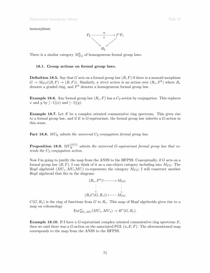
Equivariant homotopy theory Talk 18
isomorphism
F2
∼=ψ
//
f∗F1
||
R2
There is a similar category MhFG of homogeneous formal group laws.
18.1. Group actions on formal group laws.
Definition 18.5. Say that G acts on a formal group law (R,F ) if there is a monoid morphismG → MFG((R,F ) → (R,F )). Similarly, a strict action is an action over (R∗, F
h) where R∗denotes a graded ring, and F h denotes a homogeneous formal group law.
Example 18.6. Any formal group law (R∗, F ) has a C2-action by conjugation. This replacesx and y by [−1](x) and [−1](y).
Example 18.7. Let E be a complex oriented commutative ring spectrum. This gives riseto a formal group law, and if E is G-equivariant, the formal group law inherits a G-action inthis sense.
Fact 18.8. MUR admits the universal C2-conjugation formal group law.
Proposition 18.9. MU((G))R admits the universal G-equivariant formal group law that ex-
tends the C2-conjugation action.
Now I’m going to justify the map from the ANSS to the HFPSS. Conceptually, if G acts on aformal group law (R,F ), I can think of it as a one-object category including into MFG. TheHopf algebroid (MU∗,MU∗MU) co-represents the category MFG; I will construct anotherHopf algebroid that fits in the diagram:
(R∗, Fh)
//
MFG
(R∗C(G,R∗)) MFGoo
C(G,R∗) is the ring of functions from G to R∗. This map of Hopf algebroids gives rise to amap on cohomology
Ext∗∗MU∗MU (MU∗,MU∗)→ H∗(G,R∗).
Example 18.10. If I have a G-equivariant complex oriented commutative ring spectrum E,then we said there was a G-action on the associated FGL (π∗E,F ). The aforementioned mapcorresponds to the map from the ANSS to the HFPSS.
71
Equivariant homotopy theory Talk 19
18.2. Lubin-Tate formal A-modules. For any formal group law (R,F ) there is a mapZ → End(F ) taking n 7→ [n](x). Sometimes we might want to extend this to a map out ofR; in our case this helps give things a C8 action.
Theorem 18.11 (Lubin-Tate). If R is a DVR with maximal ideal π, and given f(x) thatsatisfies f(x) ≡ πx (mod x2), f(x) ≡ x2 (mod π) (e.g. f(x) = πx + x2) then there is aformal group law Ff and a map R→ End(Ff ) sending π 7→ [π](x) = f(x).
In our case, A = Z2[ζ], A∗ = A[u] for |u| = 2, then the Lubin-Tate theorem gives a formalgroup law Ff and a map A∗ → End(Ff ) sending 2 7→ [2](x), π 7→ [π](x) = f(x), and
ζ 7→ [ζ](x). The whole point is that ζ is an 8th root of unity, and [ζ](x) is an automorphismof Ff . So C8 acts on Ff as a formal group law over A∗.
The universal property guarantees a map π∗MU ((C8)) → A∗. We know that ΩO = D−1MU ((C8)).To have a map πu∗ΩO → A∗, we need to check that D maps to a unit in A∗.
There are two valuations that agree with each other. First, we know that π generates themaximal ideal so v(1−ζ) = 1, hence v(2) = 4. Second, we have a map A→ End(Ff ) sending
a 7→ [a](x), and [a](x) ≡?xd + . . . (mod (π)). The second valuation is v(a) = log2 d andv(1− ζ) = v(π) = 1. These are the same(?).
Let’s do some computations. We know that v(1 + ζ) = 1 so 1+ζ1−ζ and 1−ζ
1+ζ are units. So
v(1− ζ2) = 2, v(1 + ζ2) = 2, and v(1− ζ4) = 4.
[1− ζ](x) ≡ x2 + . . . (mod (π)). So
[ζ](x) = x+Ff [ζ − 1]
≡ x+Ff (x2 + . . . ) (mod (π))
≡ x+ x2 + . . . (mod (π))
Similarly,
[ζ2](x) ≡ x+ x4 + . . . (mod (π))
[ζ4](x) ≡ x+ x16 + . . . (mod (π))
[2](x) ≡ x24+ . . . (mod (π))
This shows that this has height 4. Recall π = 1− ζ and 2 = π4 · unit.
Talk 19: Further directions (Doug Ravenel)
19.1. Summary. The main theorem says that θj does not exist for j ≥ 7. The programis to construct a ring spectrum S−0 → Ω satisfying three properties:
(1) Detection theorem: if θj exists, we see it in π∗Ω
(2) Periodicity theorem: Σ256Ω ' Ω
(3) Gap theorem: π−2Ω = 0
72

Equivariant homotopy theory Talk 19
This implies that π254Ω = 0 and that’s where the image of θ7 lives, a contradiction. Con-structing Ω was very difficult. To do this right, we had to learn about model categories andequivariant homotopy theory, and construct the norm and the slice spectral sequence.
19.2. θ6. The case of θ6 is open. One approach is that you might be able to squeeze alittle bit more out of the periodicity theorem, going from 256 to 128; then the same argumentwould show that θ6 does not exist. Failing this, if you could study Ω or something like it andlook at π126Ω, then you could try to reach similar conclusions. These methods could onlylead to a non-existence result.
At the other end of the problem, if you’re really gutsy you could look at the Adams spectralsequence in the 126-stem and prove that the thing actually exists.
Renee: Atiyah thinks it exists, but this is just a heuristic. The Hopf invariant manifoldshave something to do with division algebras; the reason there are only three of them is thatthey correspond to division algebras. The idea is that they have something to do with specialLie algebras. You can write down Freudenthal’s magic square:
R C H O
R A1 A2 C3 F4
C A2 A2 ×A2 A5 E6
H C3 A5 D6 E7
O F4 E6 E7 E8
It takes two division algebras and outputs a Lie algebra.
The idea is that Kervaire manifolds tell you about going along the first row and down thelast column.
j 0 1 2 3 4 5 6
2j+1 RP 2 CP 2 HP2 OP2
There are three special manifolds in the remaining dimensions, of which the symmetry groupsare exactly E6, E7, and E8, respectively. I know that F4 is the symmetry group of OP2.The manifolds are called the Rosenfeld projective planes, or the bi-octonian plane, the quad-octonian plane, and the octo-octonian planes, and are denoted (O⊗C)P2, (O⊗H)P2, and (O⊗O)P2. The manifolds in the table aren’t actually Kervaire manifolds; they’re in dimensions2 higher than the Kervaire manifolds. The heuristic is actually due to Bokstedt.
The method got a manifold for θ4. Last Mike heard, θ5 hasn’t been constructed yet.
19.3. Odd-primary case.
Theorem 19.1 (Ravenel, 1978). For p ≥ 5, θj does not exist for j ≥ 2.
73

Equivariant homotopy theory Talk 19
What is θj? It corresponds to an element that lives in Ext2,2pj(p−1)A (Fp,Fp); it’s sometimes
denoted by bj . Now b1 is also known as β1; it’s the first one. Toda proved that the next one,θ2, also known as βϕ/p supports a differential that hits α1θ
p1. Then the argument in Ravenel’s
paper leverages this, but for various technical reasons it doesn’t work at the prime 3.
At p = 3, θ1 exists in the 10-stem, θ2 does not exist (Toda’s theorem), but θ3 does exist in the106-stem “by something of an accident”. Ravenel thought about this a lot, thought aboutusing all the machinery discussed in this workshop, but does not know how to constructMUR. Look at Ravenel’s slides from Banff four years ago discussing this.
If you did have MUR, the ΩO you’re looking for would be D−1NC9C3MUR; if everything worked,
you’d have a 972-dimensional periodicity theorem. The dimension of θ5 is 970. (Even infantasy land, you’re planning on leaving out θ4.) θ4 would still be unsettled. Instead ofworking at height 4, you would be working at height 6; instead of C8, it would be C9.
19.4. Differential on h2j . θj must support a nontrivial differential in the ASS and
ANSS. We have no idea what differential it is and what it hits.
19.5. EHP sequence. In the 60’s, Mahowald assumed for simplicity that the θj ’s allexist; then he had a good idea about how they fit into the EHP spectral sequence.
The following is all in the green book, §1.5.
It was proved in the 50’s by James that there are 2-local fibrations Sn → ΩSn+1 → ΩS2n+1.This leads to a LES
· · · → πn+kSn E→ πn+k+1S
n+1 H→ pπn+k+1S2n+1 P→ πn+k−1S
n → . . .
For historical charm:
• E stands for Einhangng (the German word for suspension)
• H stands for Hopf
• P stands for Whitehead product
There’s a way to combine all these LES’s to get a spectral sequence.
If k = n, πn+k+1S2n+1 = Z. Call the generator xk. It might pull back to πn+k+1S
n+1, or itmight not. If k < n then the group is zero, so the previous map is onto; this is part of theFreudenthal suspension theorem. If you have something in the k-stem, you can ask what thesmallest value of n is so that it pulls back to πn+kS
n.
For k = n, we have π2n+1S2n+1 = Z generated by xk. Let ϕ(j) =
2j j ≡ 1, 2 (mod 4)
2j + 1 j ≡ 0
2j + 2 j ≡ 3.
74

Equivariant homotopy theory Talk 19
j ϕ(j − 1)
0 0
1 1
2 3
3 7
4 8
5 9
6 11
7 15
8 16
These are the dimensions where the orthogonal group has nontrivial homotopy.
Let αj denote the generator of the image of J in dimension ϕ(j)− 1. If you have an elementin a stable stem, you pull back as far as you can; the Hopf invariant (related to the H map)is an obstruction to pulling it back further.
H(θ1) = α1 = η ∈ π1
H(θ2) = α2 = ν ∈ π3
H(θ3) = α3 = σ ∈ π7
H(θ4) = α4 ∈ π8
H(θ5) = α5 ∈ π9
H(θ6) = α6 ∈ π11
H(θ7) = α7 ∈ π15
θ4 = x22α4
θ5 = x53α5
θ6 = x115α6
θ7 = x241α7
Mahowald has some theorems about the αj ’s etc. But we know that this doesn’t happen.So what happens? Some of the αj ’s job was to correspond to θj . See Mahowald’s EHPsequence paper. Some of this is even in his metastable homotopy theory paper (“ChairmanMahowald’s little red book”). There are a lot of partial results.
The statements about θ4 and θ5 are true.
19.6. Concluding thoughts. I’m going to tell you a story about a dream I had [sometime in the 70’s] when I was attending a conference in Aarhus, Denmark in August. Thelatitude is very high, so if you go there in the summer, the sun comes up very early, whichis a problem if you’re trying to sleep. There were two people in this dream; one of them was
75

Equivariant homotopy theory Talk 19
Haynes Miller, who at the time was a young mathematician like me. The other was MichaelBarrett, who was British, and at the time he was totally obsessed with the Kervaire invariantproblem. He tried over and over to construct the θj ’s. He is the person who invented theterm “Doomsday hypothesis” for the possibility that only a finite number of θj ’s existed.
In this dream, the Kervaire invariant was a painting in an art gallery in Berkeley. It wasabstract, yellow and black. Michael Barratt persuaded Haynes and I to break into themuseum one night and steal the painting. Following Michael’s instructions we stole severalother paintings as a decoy so they wouldn’t know which one we were really after. But thepolice weren’t fooled. They didn’t know it had anything to do with the Kervaire invariant.They hired a psychic to come up with a description of a person who would want to steal it.She really got a good description of Michael Barratt’s personality. So the police tracked usdown. The last thing I remember is that the police had closed in on us and I was trying tohide under some floorboards; there was a knothole in the floorboards, and the policeman wasshining his flashlight into my eyes, and that was the sun.
76