1

This version June 25, 2014

We Are All QE-sians Now1

Takatoshi Ito2

Professor, National Graduate Institute for Policy Studies,

Project Professor, Graduate School of Public Policy, University of Tokyo, and NBER

Abstract.

The four major banks (BOJ, FRB, BOE and ECB) have adopted unconventional monetary

policy, or broadly-defined quantitative easing (QE), in the last several years. The broadly-

defined QE can be classified into comprehensive easing (CE) and pure-QE. The former is aimed

at purchasing assets of dysfunctional markets and the latter is aimed at expanding monetary

base to stimulate demands. The objective of this paper is three-fold. First, various QE adopted

by four central banks are classified into CE and pure-QE. Second, the Bank of Japan (BOJ) is a

harbinger for most QE measures in its earlier QE period of 2001-2006. Third, effects of BOJ’s

QE measures are empirically investigated with focus on the three possible transmission

channels with monthly data since January 1999. The long-term interest rate tends to be lower

and the yield curve tends to be flattened when the monetary base expands faster than nominal

GDP. The yen vis-à-vis the US dollar tends to depreciate when the Japanese monetary base

expands faster than the US monetary base. An impact of monetary base expansion on the

inflation expectation is not confirmed. Findings are consistent with a view that QE is effective,

by lowering the long-term interest rate and the currency depreciation.

JEL. E31, E43, E44, E52, E58,

Keywords: Quantitative Easing, unconventional monetary policy, inflation targeting, inflation

expectation, central bank balance sheet, zero interest rate policy

1 The earlier drafts have been presented in a session “Unconventional Monetary Policies in Crisis Times: Which Impact and What Legacy?” in the American Economic Association meeting, January 2012; and the central banking seminar, “Global Stance of Monetary Policy” at the Federal Reserve Bank of New York, October 23, 2013 and the international conference at the Bank of Japan, May 28-29, 2014. 2 The author is grateful to Professors Jan Marc Berk, Guillermo Calvo, Maurice Obstfeld, and Kazuo Ueda; as well as Messrs. Haruhiko Kuroda, Kazumasa Iwata, Hiroshi Nakaso, Paul Tucker, and other participants of the Bank of Japan conference, for their comments. However, all views and errors are mine.

2

Introduction

The interest in the effectiveness of unconventional monetary policy—sometimes

dubbed as quantitative easing (QE)—has been raised as the major central banks adopted

monetary policy with purchase of various assets, resulting in the expansion of its

monetary base, which is the dominant component of the overall balance sheet of a central

bank. The objective of this paper is two-fold. First, various policy measures in the

category of unconventional monetary policy, or broadly-defined quantitative easing (QE),

adopted by the four major central banks are reviewed and classified into sub-categories

such as credit easing (CE) and pure-quantitative easing. Second, effectiveness of

quantitative easing (QE) on the interest rate, the exchange rate, the inflation rate and the

inflation expectation will be investigated using mainly the Japanese data.

The first QE was introduced by the Bank of Japan (BoJ) in 2001 and maintained

until 2006. The period can be viewed as QE0, as it was the QE before the global financial

crisis. Many researchers, mainly Japanese, have examined how effective QE0 was, and

one broad consensus is that the QE with some forward guidance lowered the long-term

interest rate and flattened the yield curve. An overall effect on stimulating economic

growth or getting out of deflation was not debatable.

After the global financial crisis of 2007-2009, all major central banks adopted

some forms of broadly-defined QEs in order to help stabilize dysfunctional markets, to

support output activities, to avoid falling into deflation. The Bank of England (BOE)

tripled its balance sheet and the Federal Reserve System (FRB) doubled its balance sheet

in the wake of the Lehman Brothers failure. The European Central Bank (ECB) expanded

the balance sheet, but the rate of expansion was smaller than BOE or FRB. In the first

phase of crisis management, from September 2008 to the summer of 2009, FRB explicitly

mentioned that the primary purpose of asset purchase was to restore stability to the

dysfunctional markets. Thus, it should be called “credit easing” (Bernanke (2009)). The

purchase of covered bonds and lending operation by the ECB can be viewed in the same

reasoning. The size of the balance sheet became a major monetary policy tool when the

FRB adopted a large-scale asset purchase, expanding the balance sheet further in 2010.

Observers started to call it QE2, while renamed CE to QE1.

The Bank of Japan adopted a new QE, termed QQE, much later than FRB, BOE,

and ECB. The BOJ started to expand the balance sheet under the comprehensive easing

of October 2010, but the speed of expansion was much slower than other three central

banks. Only in April 2013, much later than other central banks in the post global financial

crisis, did the BOJ adopt the aggressive balance-sheet expansion.

An immediate origin of the global financial crisis that started in the summer of

3

2007 was the subprime loans problem in the United States. The loans were securitized,

bundled and re-securitized (CDOs), and sold to wide-range of investors in the United

States and Europe. As the value of securities started to decline, because the underlying

loans started to be defaulted, financial institutions started to deleverage. However, the

more institutions rush to exit from the market, the price decline accelerated and soon the

buyer simply disappeared.

Those institutions which held too much for these securities and acted slowly in

exiting from the toxic securities market increasingly found themselves short of liquidity.

Price quotes for assets were not available and no other institutions were able to lend to

such institutions. Bear Stearns was forced to be sold in March 2008, with assistance of

Federal Reserve Bank. It was a remarkable that public assistance was extended to

preserve the value of creditors to Bear Stearns. But, that was only the beginning. When

Lehman Brothers got into trouble of liquidity shortage in September, no institution was

willing to merge the institution without a large sum of public assistance, which was not

available this time from the Federal Reserve.3

In the wake of the failure of Lehman Brother, no large financial institution that

had significant securities and structured product businesses was trusted by another.

Liquidity completely dried up. Central banks and governments in US and Europe were

busy closing down or injecting capital to large financial institutions to avoid total collapse

of the financial markets. Central banks of major countries have adopted unconventional

monetary policy, that is, (near) zero interest rate policy (ZIRP) and/or quantitative easing

(QE).

As financial and real activities contracted worldwide, the major central banks—

the Federal Reserve Board (FRB), the European Central Bank (ECB), the Bank of Japan

(BOJ), and the Bank of England (BOE) adopted (near-) zero interest rate and various

measures that can be summarily called “quantitative easing” (QE). The central banks

bought kinds of assets that had not been purchased previously, with a large scale that had

not been seen earlier. The QE policy has a common feature of increasing, and maintaining

the increased, balance sheet. However, QEs of the four central banks were different in

kinds of assets they bought, the timing of adopting QE, and the scale of its QE. There are

several variants of QE policy.4

Among the different QEs, asset purchases of dysfunctional markets, which was

3 See Ito (2010) for details of what set off the global financial crisis and early stage of QEs. 4 Some authors and central banks called such operations in various names and acronyms: credit easing (CE); large scale asset purchases (LSAP), nonconventional monetary policy (NCM), unconventional monetary policy (UMP).

4

called by Chairman Bernanke “credit easing,” is widely recognized as very effective. The

pure form of QE, expanding the balance sheet by purchasing long government bonds has

mixed reviews. It tends to lower the long bond yield, but evidence on impacts on the real

activities is thin. The variant of QEs of the four central banks are still in place as of this

writing (summer of 2014), i.e., six years after the onset of the global financial crisis. We

are all QE-sians now.

The Bank of Japan had experienced zero interest rate policy (ZIRP) and

quantitative easing (QE) well before the current episode of all major central banks

adopting QE. The Bank of Japan adopted ZIRP from February to August 1999, exercising

QE with increasing the size over time, and then successfully exiting in March/July 2006.

However, when the US and European economies fell into a deep crisis after the Lehman

Brothers collapse in 2009, the Bank of Japan was the last to adopt QE among the major

four central banks. In 2009, FRB, BOE, and ECB doubled and tripled their sizes of

balance sheet. BOJ barely expanded the size of its balance sheet, resulting in large yen

appreciation. There are two possible explanations for inaction. First, by 2008, the Bank

of Japan seemed to have developed a view that the QE of 2001-06 was not very effective

in stimulating the economy or increasing the inflation rate. Second, reformed Japanese

financial institutions remain financially strong when the global financial crisis started.

Although financial institutions were strong, the Japanese economy was deep into a

recession with worsening deflation in 2009-2011, mostly due to a trade channel.

It was not until Prime Minister Abe put strong pressure on BOJ to adopt a bold

easing, that the BOJ took up QE that would rival other major central banks. On April 4,

2013, newly appointed Governor Kuroda announced Quantitative and Qualitative Easing

(QQE), which, among others, would double the size of the balance sheet in two years and

lengthen the maturity of Japanese government bonds (JGBs) they hold on the balance

sheet. An anticipation and realization of the bold B/S expansion plan is widely credited

for depreciation of the yen vis-à-vis the US dollar by 20 percent and rise of Nikkei stock

price index by more than 60 percent between mid-November 2012 and mid-May, 2013.

The inflation rate has risen from negative territory to +1.3%. This paper analyzes the

possible causes of these market reactions to QQE in light of QEs of the four major central

banks. QQE is casually regarded to be much more successful than the earlier episode of

QE by BOJ, or QEs practiced by other central banks mentioned above.

A puzzle here is why the QQE of 2013 had so strong effects in producing yen

depreciation and stock price increases, when the pure QE as opposed to CE is broadly

considered to be weak in stimulating the economy. This paper will attempt to give an

explanation for the puzzle.

5

The rest of this paper is organized as follows. Section 2 describes details of QE

measures among the four major central banks with chronology. Experiences of the four

central banks are similar in their motivations, the exact implementations of ZIRP and QE

and their effectiveness seem to be different. Most advanced economies went into a deep

recession in the wake of the global financial crisis. Section 3 shows the movements of

balance sheets of the four major banks. Section 4 describes the transmission channels.

Section 5 first describes movements of the exchange rate and the stock prices after Prime

Minister Abe started to campaign for lifting the Japanese economy out of deflation. Some

evidence will be presented in that monetary base expansion tends to cause currency

depreciation. The changes of the Phillips curve position and slope will be also examined.

This section will be a main contribution of the paper. On Section 6 concludes the paper.

1. Chronology and Taxonomy

1.1. Bank of Japan

1.1.1. Early ZIRP and QE, 1999-2006

In the wake of Japanese banking crisis of 1997-98 and rapidly declining output

and declining prices in 1998, the BOJ decided to lower the policy rate (call rate) to zero

in February 1999. This is the first case of the zero interest policy (ZIRP) among major

central banks (with a possible exception of the Swiss Central Bank in the 1970s).

However, the policy rate was raised by 0.25% in August 2000. The decision to end ZIRP

was controversial. Two votes were against this decision. The government representatives,

who are by law non-voting, requested to delay the vote of raising the interest rate until

the next meeting, according to the procedure allowed to the government representative.

The delay request was overruled by voting members of Monetary Policy Meeting

(MPM).5 The inflation rate was still negative at the time of decision and the global

economy started to slow down due to the IT bubble burst.

The economy did not improve, and in March 2001, the Bank of Japan adopted a

new instrument target, current account balance (CAB) at the Bank of Japan, which is the

account that banks have their required and excess reserves. This is the beginning of

quantitative easing (QE) in Japan. Since the required reserves did not change significantly,

targeting the current account balance meant targeting the amount of excess reserves. Since

the excess reserves were not paid interest at the time, targeting the amount of excess

reserves means that the interbank rate (which is the policy rate) becomes zero. On the

asset side, the Bank of Japan started to increase the amount of monthly purchase of

Japanese Government bonds (JGBs). The amount of long-term bond purchase and the

5 See Ito (2004a) for a controversial decision in August 2000.

6

target amount of CAB increased as the Japanese economy could not get out of deflation.

The QE continued until March 2006, when the instrument target was switched back to the

(zero) interest rate. After lowering the CAB from 35 trillion yen to 6 trillion yen in several

months, the BOJ was ready to exit. The interest rate was raised by 0.25% in July 2006.

Since reserves in CAB were not renumerated, reducing the amount of excess reserves to

minimum was necessary to raise the interest rate. This was done between March and July

of 2006. Since most of the long bonds purchased by the Bank of Japan had shorter

maturity, the process of reducing the size of CAB was rather smooth.

Amid worsening of global financial stability in the weeks following the collapse

of Lehman Brothers, the Bank of Japan did not expand the balance sheet. The policy

interest rate was cut from 0.5% to 0.3% in October and then to 0.1 percent in December

2008. It participated in the US dollar swap among the G10 countries. There was no

decision on aspects on quantitative easing. The rate cut in October was decided by tie-

breaking vote by the Chair of MPM (Governor). The BOJ in the wake of the Lehman

Brothers failure had a view that the Japanese financial markets and economy could not

be adversely affected by the global financial crisis, which would warrant some type of

QE.

It was not until October 2010 that a version of QE was introduced by BOJ. In

announcing “comprehensive easing,” the BOJ introduced a special, temporary program

that purchases assets and provides liquidity with fixed-rate, funds-supplying operation.

The asset purchase part is 5 trillion yen and funding operation by 30 trillion yen, a total

of 35 trillion yen. The maturity of assets to purchase ranges between 1 and 2 years. The

asset purchase program (APP) is on the balance sheet but deemed temporary. The reason

for creating the program was to make an exception to an earlier self-imposed rule that the

amount of long bonds held by the Bank of Japan should be less than the amount of bank

note issues. The amount of APP was increased to 91 trillion yen in several steps by

October 30, 2012. On that day, the government and BOJ signed a joint statement that both

would cooperate toward overcoming deflation.

On January 22, the government and BOJ signed another document, in which the

inflation “goal” should be around 1 percent. The market welcomed the document,

generating yen depreciation and stock price increases, believing that this would lead to

more aggressive easing. However, it was not clarified having the goal leads to a different

policy, and the market reverted to the pre-announcement levels.

As the economy showed the sign of weakness, the government started to put

pressure on the BOJ in mid-2012. This resulted in the October 30 document, signed by

Governor Shirakawa, Finance Minister Jojima and Minister of State for Economic and

7

Fiscal Policy Maehara. The statement called for ending deflation, reiterating the

importance of 1 percent inflation goal.

In the mid-November, the House of Representatives was dissolved and the

general election was to be held in mid-December. This turned out to become the beginning

of the change in monetary policy and the relationship between the government and the

BOJ.

1.1.2. QQE

Mr. Abe, then a leader of the opposition party, started to advocate aggressive monetary

policy in mid-November 2012 as a part of platform for the general election that was to be

held in December 16, 2012. Mr. Abe won the general election and became Prime Minister

on December 26, 2012.

Mr. Abe argued that ending the long-lasting deflation—negative inflation rates

for 15 years except several months—as a key to revive the stagnant economy. In order to

raise the inflation rate, adopting 2% inflation targeting and aggressive monetary policy

were essential. The Bank of Japan and the government signed the document that the Bank

will pursue the 2% inflation targeting in January 2013. At the expiration of Governor

Shirakawa’s term, Mr. Abe appointed Mr. Kuroda, who was regarded by the market to be

sympathetic to the idea of inflation targeting and credible to pursue strong measures to

end deflation. Mr. Kuroda announced the quantitative and qualitative easing (QQE) at the

end of his first monetary policy committee meeting, on April 2014.

The QQE policy had the following elements.6 First, it reiterated the 2 percent

inflation target of monetary policy, “at the earliest possible time, with a time horizon of

about two years.” In order to achieve this, the BOJ “will double the monetary base and the

amounts outstanding of Japanese government bonds (JGBs) as well as exchange-traded funds

(ETFs) in two years, and more than double the average remaining maturity of JGB purchases.”

The monetary base was chosen as a main operating target, and the BOJ “will conduct money

market operations so that the monetary base will increase at an annual pace of about 60-70

trillion yen.” This is the “quantitative” part of the QQE. Regarding type of assets to buy, the

BOJ “With a view to encouraging a further decline in interest rates across the yield curve, the

Bank will purchase JGBs so that their amount outstanding will increase at an annual pace of

about 50 trillion yen.” It also specified that JGBs to be purchased is “JGBs with all maturities

including 40-year bonds will be made eligible for purchase, and the average remaining

6 The quotations in this paragraph is from the Bank of Japan, “Introduction of the "Quantitative and Qualitative Monetary Easing” April 4, 2013. http://www.boj.or.jp/en/announcements/release_2013/k130404a.pdf

8

maturity of the Bank's JGB purchases will be extended from slightly less than three years at

present to about seven years.” In addition, purchases of ETFs and J-REITs are expanded:

“With a view to lowering risk premia of asset prices, the Bank will purchase ETFs and Japan

real estate investment trusts (J-REITs) so that their amounts outstanding will increase at an

annual pace of 1 trillion yen and 30 billion yen respectively.” The lengthening of JGB

maturity and expanded purchase of ETF and J-REIT are the “qualitative” part. Although JGB,

ETF, and J-REITs have been bought under APP that was introduced under the comprehensive

easing of December 2010, the QQE abolished the APP and absorbed the assets on the regular

balance sheet of BOJ, but suspending the “banknote principle,” a limiting the JGB holding

under the size of banknote issues.

The amount of balance sheet expansion plan is much larger than the market

expected, and absorbing temporary APP in the general balance sheet gave an impression

that the balance sheet gave an impression that quantitative easing of this scale will

definitely continue until the 2 percent inflation targeting will be achieved. Lengthening the

maturity of JGBs is also a key contributing to a rapid increase of the balance sheet. Under

APP, only short-maturity government bonds and bills were purchased.

1.2. Federal Reserve Board

The Federal Reserve Board (FRB) decided to start buying private securities

under various facilities, which later be named as “credit easing” in January 2009 by

Bernanke (2009). Credit easing was designed to intervene in dysfunctional markets due

to liquidity dry-up, caused by severe informational uncertainty. The Federal Reserve acted

as a buyer of the last resort. Bernanke (2009) explained the difference between his policy

and BOJ’s policy from 2001 to 2006 as follows.

“The Federal Reserve's approach to supporting credit markets is conceptually

distinct from quantitative easing (QE), the policy approach used by the Bank

of Japan from 2001 to 2006. Our approach--which could be described as

"credit easing"—resembles quantitative easing in one respect: It involves an

expansion of the central bank's balance sheet. However, in a pure QE regime,

the focus of policy is the quantity of bank reserves, which are liabilities of the

central bank; the composition of loans and securities on the asset side of the

central bank's balance sheet is incidental. Indeed, although the Bank of

Japan's policy approach during the QE period was quite multifaceted, the

overall stance of its policy was gauged primarily in terms of its target for bank

reserves. In contrast, the Federal Reserve's credit easing approach focuses on

the mix of loans and securities that it holds and on how this composition of

9

assets affects credit conditions for households and businesses.” (Bernanke

(2009))

Bernanke seems to emphasize the difference between the FRB policy and the

Bank of Japan policy targeting the amount of reserves (current account balance). In this,

The balance sheet quickly doubled in several months. Increasingly, the Federal Reserve

bought Mortgage Backed Securities (MBS). The acute phase of financial crisis ended by

late 2009. The FRB stopped new purchases of MBS, as the initial goal was achieved in

March 2010. However, the GDP gap had become large and the inflation rate had come

down significantly. In order to maintain stimulus posture, the FRB decided to maintain

the size of balance sheet, by replacing the maturing (and early repayments of) MBS with

new purchase of Treasury bonds.

The decision to maintain the level of B/S was made on August 2010. This is the

timing of change from CE to QE. In November the so-called QE II, increasing the size of

B/S by buying Treasury bonds. However, the switch from CE, buying securities of

dysfunctional markets only, to QE, the size of B/S matters, occurred in August rather than

November of 2010.

The QE-2 ended in June 2011. The Federal Reserve never uses QE, describing

their policy to expand the B/S. Instead, they call large-scale asset purchases (LSAP).

However, here we interchangeably use QE and LSAP. The expansion of B/S was

remarkable, but with an increasing criticism too, as measurable improvement was not

observed. In September 2011, the so-called operation twist, selling the short-term

Treasury bills are sold and long-term bonds were purchased, without significantly

changing the size of B/S.

The so-called QE-3 was initiated in September 2012, without specified ending

date or total amount of purchase. It specified the amount of monthly purchases.

1.3. ECB

The ECB’s non-standard measures include three stages: The first stage to

alleviate liquidity shortage by providing longer term funding; the second stage to

purchase covered bonds; the third stage to purchase government bonds of countries that

are hit by European sovereign debt crises; and the fourth stage to announce a defense of

the euro.7

7 This section draws from ECB publications, in particular, for the early part of the crisis, see European Central Bank, “The ECB’s Response to the Financial Crisis,” Monthly Bulletin, October 2010, pp.59-74.

10

When the global financial markets experienced liquidity shortage from the

summer of 2008, many European institutions, along with the US institutions, attempted

to deleverage. The shortage of liquidity in the euro zone was severe, and the European

Central Bank (ECB) provided liquidity first through their conventional channel by

lowering the policy rates, but expanded the tools to longer funding. ECB Governing

Council decided in October 2008 to increase the frequency and size of its longer-term

(with a maturity of up to six month) refinancing operations; to conduct all liquidity-

providing operations through a fixed rate tender procedure with full allotment; and to

provide US dollar and Swiss franc via swaps.

In May 2009, the ECB decided to provide longer term (12 months) funding and

to purchase euro-denominated covered bonds issued in the euro area. Purchasing of

covered bonds were described by ECB as follows: “This measure aims to improve

liquidity in the private debt security markets and encourage a further easing of credit

conditions given that the deleveraging process in the banking sector, which has recently

accelerated, is likely to continue for some time. Specifically, covered bond purchases in

both primary and secondary markets should improve the funding conditions for financial

institutions that issue covered bonds in the primary market. Covered bond purchases in

the secondary market should contribute to improving the depth and liquidity of the market

and should further narrow the spreads of covered bond yields over those on government

bonds. This should improve the risk profile of institutions holding covered bonds and

thereby help to spur credit growth. Furthermore, covered bond purchases could encourage

new issuances in the primary market and contribute to activity in the secondary market,

which has remained subdued.”8 Purchasing covered bonds are targeted to ease credit

conditions of these bonds, and as a result to ease liquidity conditions of banks in the euro

zone. Indeed the decision was justified on the ground of ECB’s support to the banking

system. This may be comparable, with a narrower scope, to operations by FRB to

purchase private sector’s debts several months earlier in the United States, which

Chairman Bernanke called credit easing.

The size of covered bond purchases, decided on June 4, 2009 was 60 billion euro.

One of the conditions for bonds eligible for purchase was AA-rated or above by at least

one of the major rating agencies (Fitch, Moody’s, S&P or DBRS).

The Euro zone financial markets were hit by a crisis of sovereign debts in 2010-

11. The euro-zone sovereign debt markets were affected in months following the Lehman

Brothers’ failure. However, the situation was under control toward the summer of 2009.

The debt yield started to climb up again after the Greek government’s announcement in

8 European Central Bank, Monthly Bulletin, June 2009, p. 10.

11

November 2009. Greek government revealed that it had much larger government deficits

(12.7% of GDP) than earlier reported. The sovereign debt yields of these countries went

up to a level that a crisis will become self-enforcing.

In May 2010, the IMF, ECB and EU (troika) agreed with the Greek government

that the troika provide financial assistance to Greece in return for structural adjustment.

On May 10, 2010, the ECB announced a new policy called “Securities Markets

Programme” (SMP), in that the ECB purchases purchase public and private debt

securities in the euro area to ensure depth and liquidity in those market segments. The

ECB stated that the objective is to restore an appropriate monetary policy transmission

mechanism. This also is to restore liquidity to dysfunctional markets, which this time

include sovereign debts. The operation is not in the type of quantitative easing because

these purchase is sterilized through specific operations to re-absorb the liquidity injected.

The sovereign debt yield spread (over the German bonds) for GIIPS temporarily

fell after the measures in May 2010, but it resumed accent soon after. Once the Greek

situation was in focus, the investors started to sell securities in countries that had relatively

bad government debt and financing situations: Greece, Italy, Spain, Portugal, and Ireland

(GIIPS). In August 2011, the yield spreads of ten year bonds for Greece, Portugal, and

Ireland reached more than 800 basis points. ECB re-started SMP operations in August

2011 and continued until September 2012. In addition, in December 2011, the Long Term

Refinancing Operations (LTRO) was announced and done. With these measures, the yield

spreads narrowed and the crisis was headed off.

On August 2, 2012, the ECB announced that the ECB is ready to purchase

sovereign bonds in outright monetary transactions (OMT) if necessary to protect the euro

from disintegration. Details of OMT were announced in September and SMP was

terminated. The OMT was placed as an ultimate measures to defend the euro with open

ended commitment to purchase debts. However, it was designed to purchase of

government bonds of countries that require IMF programs (including precautionary ones)

with conditionality. It is emphasized in the statement that OMT will be fully sterilized.

OMT has not been used so far. This is not pure-QE in the sense that it is not intended to

expand the balance sheet of ECB. 9 It was reported that Bundesbank and German

government were against ECB's bond-buying plan, as it was regarded to erode "the

willingness of Eurozone member-states to implement reforms."

But, in the second half of 2012, the sovereign bond spreads (over German’s

9 See "Technical features of Outright Monetary Transactions", ECB Press Release, 6 September 2012.

12

yield) went down significantly. Many attributed this to OMT.

In sum, ECB operations—Covered bond purchases, LTRO, SMP, and OMT—

were said to be targeted to restore liquidity and depth in the market. Effectively, SMPs

helped yield spreads of government bonds of the crisis hit countries come down. Also,

OMT announcement had a similar effect. The quantitative easing in the sense of

expanding the balance sheet itself was not mentioned, and it was specifically mentioned

that SMP and OMT would be sterilized. However, the expansion of balance sheet did

occur through easier market conditions, via covered bond purchases and LTROs, at least

in the beginning stage of the global financial crisis.

In the spring of 2014, President Draghi suggested that monetary easing may be

needed to curtail the exchange rate appreciation. It was widely received by the financial

market participants that the ECB may be considering quantitative easing.

1.4.BOE

Between March 2009 and January 2010, BOE purchased £200 billion of assets,

mostly medium and long-dated gilts. These asset purchases amounted to purchase of

nearly 30% of the outstanding gilts held by the private sector. Combined with earlier

liquidity support measures to the banking sector, the size of the Bank’s balance sheet in

ratio of GDP tripled compared with the pre-crisis period. This was the first phase of

quantitative easing for the BOE, namely QE-1.

The BOE restarted the QE on October 6, 2011 by announcing the increase in the

size of the purchase program by £75 billion to a total of £275 billion. The expansion

continued in steps. In February 2012, the size was expanded by £50 billion to a total of

£325 billion, and then expanded again in July 2012 by £50 billion to a total of £375 billion.

The BOE, unlike ECB, did not hesitate purchasing long government bonds; and

unlike BOJ and FRB, it did not buy private sector’s assets. The BOE’s policy represents

a pure form of QE.

1.5. Taxonomy

As reviewed above, broadly-defined QE has indeed two types: one that are

targeted to stability dysfunctional financial markets, credit easing, and narrowly-defined

QE, or pure-QE, that aims at (some components) of the balance sheet.10

10 Ueda (2013) also presented taxonomy. He categorizes non-conventional policy of BOJ and FRB into “forward guidance,” “LSAP1,” “LSAP1” and “QE.” QE is the policy adopted by BOJ from 2001-2006.”. Then, he critically reviews most recent events. He examines the possible logic of a view that adopting inflation targeting with aggressive monetary policy works to stimulate aggregate demand and eventually raise the

13

The CE operations include programs that purchase either public or private assets

where markets are dysfunctional, i.e., liquidity and pricing are deemed abnormal. The CE

(or QE-1) of FRB in 2008-2009 and ECB purchase of covered bonds and sovereign bonds

(SMP and OMT when implemented) belong to this category. The FRB’s purchase of MBS

under QE-3 is also in this category. The FRB operation twist, changing composition of

assets without changing the size of balance sheet belongs to this category.

The BOJ’s QE from 2001 to 2006 and BOE’s QEs belong to narrowly-defined

QE. So is FRB’s QE-2 and BOE’s QEs.

The qualitative part of QQE introduced by BOJ is of CE-type and the “qualitative”

part of QQE is of pure-QE type. The FRB’s QE-3 also has a CE-type (purchase of MBS)

and QE-type (purchase of Government bonds). Table 1 summarizes this taxonomy.

<Insert Table 1 about here>

2. We are all QE-sians now

Most measures taken by the four major central banks that are described above meant their

balance sheets (B/S) expand, although their stated objectives and transmission channels

are different. In the period of global financial crisis, the balance sheet movement is shown

in Figure 1.

<Figure 1 about here>

The BOE balance sheets rose most among the four. Compared to the pre-crisis level, it

tripled within a few months following the Lehman Brothers collapse. The level stayed at

around 300% of pre-crisis level from mid-2009 to late 2011. Due to its QE-2 and QE-3,

the level as of May 2014 is about 500% of the pre-crisis level.

FRB has increase its balance sheet in steps, CE, QE-2, and QE-3. The QE-3 has

been open-ended but it is slowing down in 2014 as a result of tapering. By the end of

2014, the growth of balance sheets will stop. The resulting level of QE will be similar to

the one of BOE, namely the 500% of the pre-crisis level.

ECB has been reluctant in expanding the balance sheet for its sake. The

outstanding balance of SMP, in which government bonds of member countries have been

purchased, has been “sterilized.” OMT has not been activated, to that it has not

contributed to the balance sheet. The balance increased in the weeks immediately

following the Lehman Brothers collapse, and then from mid-2011 to mid-2012. The peak

level was about 280 percent of the pre-crisis level.

BOJ did not expand the balance sheet in the wake of the Lehman Brothers,

despite other thee banks increased the balance sheet—BOE three times, FRB twice, and

inflation rate, within two years as the inflation targeting policy sets out.

14

ECB by 50%. The BOJ balance sheet was basically flat until October 2010, the time of

comprehensive easing. Although wide-ranging asset purchases were announced, its

impact on the balance sheet was small compared to other three central banks. Only after

QQE was introduced in April 2013, the BOJ balance sheet started to increase measurably.

By the end of 2013, the increase in BOJ balance sheet (in ratio to pre-crisis level) overtook

the ECB balance sheet. Under QQE, the BOJ had committed to double the size of

monetary base, which is closely tied to the size of balance sheet, in two years. Therefore,

it is projected until the end of March 2015. Even at the end of two-year QQE commitment,

the increase in size of balance sheet (in ratio to pre-crisis level) of BOJ is about the half

of BOE and FRB, but higher than ECB.

3. Transmission Channels

3.1. Objectives

Price stability as a primary objective has become standard in monetary policy among

advanced and emerging market countries. Many central banks have explicitly adopted

(flexible) inflation targeting (FIT) and others have been practicing without declaring it.

BOE has adopted inflation targeting since 1992. Between mid-1990s and mid-2000s,

central banks of many advanced countries and emerging market economies have adopted

FIT. The US Federal Reserve Board and Bank of Japan were late comers to embrace FIT.

The FRB adopted in January 2012, but it had practiced it without declaring it for several

years before the formal declaration. The BOJ adopted FIT in January 2013. The fact FRB

and BOJ adopted inflation targeting after the global financial crisis occurred is suggestive

that FIT is actually helpful in maintaining the inflation expectation anchored (continued

to be anchored in FRB and newly anchored in BOJ) so that achieving price stability is

easier with FIT than without.

Regarding additional objectives (or mandates), central banking laws and

practices vary across countries. Achieving maximum output, or minimizing output gap,

is implicitly or explicitly recognized as an additional objective. Also, the stability of

financial markets and institutions are written sometimes explicitly and sometimes

implicitly.

Keeping output gap smaller (achieving potential output) and keeping financial

markets stable have been frequently mentioned as additional objectives or as

preconditions to price stability. Hence, central banks with these additional objectives

found it easier to implement QE, in particular in the form of CE, since measures can be

easily justified and explained to the legislature and general public. In some quarters of

central banking, the single mandate of price stability is the best to keep independence of

15

the central bank and monetary dominance. However, my interpretation of the recent crisis

evolution is that the global financial crisis revealed that explicit mention of financial

market stability and output stability may be useful additional mandates to have in a crisis,

as explained below.

The Federal Reserve have been created with “dual mandate,” namely price

stability and maximum employment. The regularly scheduled testimony by Chairman of

the Federal Reserve Board to the Congress always emphasize the two mandates.

The Bank of Japan law also mentions that “the maintenance of stability of the

financial system” (Article 1-(2)) is the Bank’s purpose. Article 2 states: Currency and

monetary control by the Bank of Japan shall be aimed at achieving price stability, thereby

contributing to the sound development of the national economy.” This article is intended

to prevent the Bank to pursue price stability single-mindedly, if output activities are

continuously stagnant and output potential is not realized for a sustained period.

Before the global financial crisis of 2008-09, price stability and financial

systemic stability were separated between the Bank of England and Financial Services

Authority (UK FSA), respectively. However, after the global financial crisis subsided, the

UK government decided to move back the role of financial stability back to the Bank of

England.

The treaty that established ECB has articles that prohibit a bail-out of the

government and monetary financing of the government (Articles 125 and 123 of the

Lisbon Treaty).11 There has been a controversy within Euro Zone countries over SMP

and OMT due to these articles. ECB’s hesitation of buying government bonds for any

purpose reflects the controversy.

Is it easier for a central bank with additional mandates (output, financial stability)

to practice QE? When financial stability is explicitly mentioned as a mandate, it is quite

easier for a central bank of intervene in the dysfunctional market. However, financial

stability was an overwhelming concern at the most acute stage of global financial crisis, 11 Article 123. 1. Overdraft facilities or any other type of credit facility with the European Central Bank or with the central banks of the Member States (hereinafter referred to as ‘national central banks’) in favour of Union institutions, bodies, offices or agencies, central governments, regional, local or other public authorities, other bodies governed by public law, or public undertakings of Member States shall be prohibited, as shall the purchase directly from them by the European Central Bank or national central banks of debt instruments. Article 125. 1. The Union shall not be liable for or assume the commitments of central governments, regional, local or other public authorities, other bodies governed by public law, or public undertakings of any Member State, without prejudice to mutual financial guarantees for the joint execution of a specific project. A Member State shall not be liable for or assume the commitments of central governments, regional, local or other public authorities, other bodies governed by public law, or public undertakings of another Member State, without prejudice to mutual financial guarantees for the joint execution of a specific project.

16

from September 2008 to the spring of 2009, whether the financial stability objective is

explicitly written in the law was not a problem. In fact, the shock was so large to the US,

UK, and Euro-zone financial institutions, interventions were justifiable even on the price-

stability objective alone. This was the case in the Bank of England. However, in the

recovery phase after the sharp downturn, having additional objectives seemed to have

helped Federal Reserve pursue more aggressive QE.

3.2. Transmission Channels

Transmission channels under QE are similar to those of conventional monetary

policy, but the instruments are different and theoretical prediction may be different.

Instead of adjusting the policy interest rate, expanding the balance sheet by purchasing

assets is purchases. Purchases of assets from the private sector are likely to cause the

portfolio rebalance among household and institutional investors. Moreover, when the

purchased assets are long-term bonds, the long-term bond yield is expected to decline.

This is more direct demand-supply relationship than purchasing short-term assets with a

forward guidance with a commitment to keep the low interest rate longer. When those

who sell long bonds and other assets to the central bank purchase riskier assets, such as

foreign assets and equities, the exchange rate is expected to depreciate and equity prices

are expected to rise. Then, wealth effects for those who hold foreign assets and equities

will increase consumption and investment spending. Chairman Bernanke and President

Mario Draghi do not hesitate to admit that any of the above mentioned channels, including

the exchange rate channel, would work, although exactly by how much is not clear.

So, let us examine the following four channels. The first channel is to lower the

long-term interest rate. This can be done either by “forward guidance” and buying long-

term government bonds. The forward guidance includes verbal commitments of keeping

the zero interest rate policy for a long time (longer than other wise) or show economic

conditions (threshold of the inflation rate or the unemployment rate) that would trigger

the rate hike, or both. The forward guidance works through changing expectations of

future policy (short) rate. Purchasing long government bonds by the central bank has a

direct impacts through changing demand and supply of the bond market.

The second channel is the exchange rate. Under the conventional regime, the

lower interest rate policy tends to result in currency depreciation through capital flows

that pursue the interest rate differential. Depreciation tends to make exports to grow and

imports to be replaced by domestic production. So this helps the economy to grow. A

question is whether QE can generate depreciation even when the interest rate is stuck at

zero. Expansion of balance sheet means liquidity is provided to the private sector, which

17

causes the portfolio rebalance. When newly acquired assets by residents include foreign

assets, the exchange rate depreciates.

The third transmission channel is through higher asset prices. Asset prices tend

to rise when the interest rate declines and households and firms are encouraged to take

more risk. QE and forward guidance are designed to produce portfolio rebalance among

assets of households, corporations and financial institutions. Once asset prices becomes

higher, consumption and investment will be stimulated.

The fourth transmission channel is the expectation channel. Adopting QE,

especially when accompanied by explicit inflation targeting can influence on inflation

expectation. In addition, when inflation expectation is not anchored at the desirable rate

of inflation, enhancing credibility by adopting an inflation targeting framework

contributes to influences inflation expectation. Adoption of inflation targeting by FRB

and BOJ is a good example.

These channels are summarized in Figure 2.

<Figure 2 about here>

3.3.Effectiveness of QE: Literature Review

Borio and Disyatat (2009) provided a taxonomy, a detailed discussion of

transmission mechanism and evaluation of various policies of advanced countries.

Reviewing experiences of various countries, they conclude the credit easing policy (CE-

type) has been effective, just expanding the monetary base (or specifically, excess reserve)

is not effective. There is no sign of an increase in bank lending. They take the BOJ

experience of QE, 2001-06 as an example. Likewise,

Ugai (2007) presents a comprehensive survey for the period of BOJ ZIRP and

QE, from 1999 to 2006. He examined the literature according to the different transmission

channels. According to Ugai (2007), the followings have become a conventional wisdom:

First, for the forward guidance (policy duration) effect on the lowering the yield curve is

consistently confirmed by Baba, et al. (2005), Oda and Ueda (2007), Okina and

Shiratsuka (2004), and Bernanke, Reinhart and Sack (2004). Second, An increase in CAB

(excess reserves) on JGBs does not have a direct effect, but has a signaling effect on the

yield is confirmed (Oda and Ueda (2007)). Third, Kimura and Small (2006) showed that

in the expanding balance sheet policy, corporate bond yield was lowered and the yen

depreciated. However, they showed that QE impacts on the stock prices and low-grade

corporate bond prices had opposite signs. Fourth, the literature is divided over effects of

CAB of 2001-2006 on the inflation rate, GDP and industrial production. Kimura et al.

(2003) found no macroeconomic effect; Fujiwara (2006) found again insignificant effects

18

on inflation, but mixed results on industrial production.

In sum, for BOJ policy from 2001 to 2006, a commitment of keeping the ZIRP

longer than normal had an effect of shifting the yield curve lower. It was at the time called

a “policy duration effect.” QE has lowered funding costs of corporate funding costs. It is

equivalent to what is called forward guidance now. The portfolio rebalancing effects was

found either small or insignificant. Whether QE has effects on growth or inflation was

not conclusively determined from the data.

On the forward guidance, the earliest contribution of suggesting the value of

commitment to future inflation in order to change expectation was Krugman (1998).

Bernanke and Reinhart (2004) identified the transmission channels of portfolio rebalance

and expectations. In addition, they also argued that purchasing of government bonds will

shift the future inflation tax burden from the public to the central bank.

Krishnamurthy and Vissing-Jorgensen (2011) examined FRB’s QE policy on the

interest rates. With an event-study they examined the interest rate reactions to policy

changes during the period of CE (i.e., QE-1) and QE-2. They have found effects on

interest rates of private securities as well as Treasuries. In particular, they found the long

government rates had responded both in QE-1 and QE-2. Gagnon, Raskin, Remache, and

Sack (2011) also found that the long-term interest rates of Treasuries and private bonds

did become lower, upon markets receiving news (hints and announcement) of large-scale

asset purchases based on a careful event-study. They also conducted time-series analysis,

controlling unemployment, CPI, and bond supply conditions, and found that the long

bond yields came down with Federal Reserve purchases of long-bonds in a sample period

from December 1986 to June 2008.

Hamilton and Wu (2012) argued that even changing the maturity structure of

FRB holdings of Treasuries can influence the long-term yield, implying that an operation

twist (selling short bonds and purchasing the same amount of long bonds) could lower

the long-term interest rate. Swanson and Williams (2013) also examined the differential

impacts of QE on medium and long term interest rates.

Gambacorta, Hofmann; and Peersman, (2014) examined unconventional

monetary policies of eight advanced countries in the post-global financial crisis with

panel VAR. They found that the expansion of the balance-sheet generates temporary

increases in economic activities and consumer prices. Impacts on economic activities

were as large as conventional measures, while impacts on consumer prices are weaker

and less persistent.

Ueda (2012a, 2012b, 2013) reviewed the BOJ policy changes—ZIRP and QE—

of the period from 1999 to 2011. He classified BOJ policy decisions during the period

19

into four types: (1) management of expectation, that is, forward guidance; (2) targeted

assets purchases in the dysfunctional market (US-QE1) and large scale asset purchases

with intention of portfolio rebalancing (QE2); and (3) Expansion of balance sheet by

purchasing short term Treasury bills. Then he conducted an event study examining

reactions of the yen-dollar, the stock prices, and various interest rates, around the

announcement dates, with a window of before-and-after changes for either 2 days or 1

week. He concluded that forward guidance and targeted asset purchases were effective in

lowering the interest rate and raising stock prices. The results on the exchange rate wer

mixed. The results are consistent with a detailed study in Oda and Ueda (2007).

Takeda and Yajima (2013) examined effectiveness of BOJ QE from 2001 to2006,

using a VAR model. They classified QE into types of providing liquidity with CAB, of

providing liquidities in the market, of purchasing assets and of expanding balance sheet.

The market variables in their analysis included the yen/dollar exchange rate, stock prices,

JGB, and other market yield spreads. Stock prices were shown to respond positively to

the CAB expansion, but long bond purchases negatively to the CAB expansion. Overall

results are not really conclusive. Some measures produced results contrary to prediction.

4. Abenomics12

The economic policy package of Prime Minister Abe is nicknamed as “Abenomics.” It

has three arrows: First, aggressive monetary policy and inflation targeting; second,

flexible fiscal policy; and third, growth strategy. The QQE introduced by Governor

Kuroda on April 4, 2013 is an important part of the first arrow.

This section is an overview of impacts of the first arrow of Abenomics on the

financial markets and macro-economy. Figures 3 and 4 show the reactions of the

exchange rate (nominal yen-dollar rate) and the stock prices (Nikkei 225), respectively.

Several political and economic events are written in the figures.

<Figures 3 and 4 about here>

There are several remarkable points that are shown in these figures. First, the

reactions of the exchange rate and the Nikkei stock prices were large. Between mid-

November 2012 and mid-May 2013, the yen depreciated by more than 20%, and the stock

prices rose more than 60%. Second, two-thirds of the climb occurred before the QQE was

announced on April 4, 2013. Third, the yen-dollar exchange rate and the Nikkei stock

prices have stayed in the box ranges since May 2013 to time of this writing (May 2014).

The first sign of changes came even before Mr. Abe became prime minister. The

House of Representatives (the lower house) was dissolved on Nov. 16, and investors in

12 This section draws on Ito (2013a).

20

the foreign exchange and stock markets immediately forecasted that the Liberal

Democratic Party (LDP) would win in the general election to be held within a month.

Thus, the yen/dollar rate and stock prices started to react to what Mr. Abe, then the

opposition leader, had to say about his economic policy. On the day before the dissolution,

the yen/dollar rate was 81 yen and the Nikkei 225 stock index was at 8,830 yen.

During the election campaign, Mr. Abe emphasized the need to reform the Bank

of Japan (BOJ), which had allowed deflation to continue for 15 years. Between mid-

November 2012 and mid-January 2013, he had been consistent and insistent in calling for

a drastic change in Bank of Japan’s policy. Earlier The Bank of Japan had agreed to “a

1% goal” in February 2012, but Mr. Abe said that it was not enough and “a 2% target”

has to be introduced. The BOJ had resisted against a proposition of an inflation targeting

framework since the beginning of ZIRP 1999 (Ito (2004a).

The market gradually believed the plausibility of such steps, especially after the

general election on Dec. 16 which the Abe-led LDP won. Mr. Abe became Prime Minister

on December 26. As prime minister, Abe has continued his campaign for a 2% inflation

target and aggressive monetary easing.

After some strong verbal persuasion coming from Prime Minister Abe, the BOJ

agreed to sign a document on January 25, 2013 to declare that the BOJ would take the

2% CPI inflation rate as a policy target. By this time, the yen had depreciated by 11% to

91 yen and the Nikkei stock index had risen by 24% to 10,927, without any change in the

BOJ policy in terms of large-scale asset purchases. Only talk and expectation had could

produce such changes. The yen depreciated without any foreign exchange intervention

and ahead of a massive expansion of the balance sheet of the BOJ.

Then Prime Minister Abe started to call for the appointment of a person who

would support his idea of inflation targeting and aggressive quantitative easing upon

expiration of the then governor’s term. Eventually, he selected Haruhiko Kuroda, then

president of the Asian Development Bank, as new BOJ governor. The first Monetary

Policy Board meeting under Governor Kuroda took place on April 3-4, 2013, with policy

changes announced on April 4. Governor Kuroda explained the new policy, termed

“Quantitative and Qualitative Easing” (QQE), at a press conference with charts in efforts

to improve on the communication front. On April 4, the stock index closed at 12,635,

some 43% up from Nov. 15; and the yen was at 96 yen/dollar, a 16% depreciation since

the same date.

The market was impressed by QQE and the yen would further depreciate and the

stock prices would continue rising. On May 9, the yen/dollar rate crossed the 100

yen/dollar line. Stock prices continued to rise and the yen continued to depreciate. On

21

May 22, the Nikkei 225 closed at 15,627 yen (up 77% since Nov. 15), and the exchange

rate became 103 yen/dollar (a 21% depreciation).

On May 22, a hit of “tapering”– that is reducing the pace of asset purchases by

the Federal Reserve – was expressed by Chairman Ben Bernanke in the United States.

The yen started to appreciate and world-wide stock prices started to decline. By mid-June,

the yen and stock prices returned to the level of April 4. Some critics argued that a mini

bubble caused by QQE was over. However, the yen again depreciated to 100 yen/dollar

and the Nikkei 225 index rose above 14,000 yen. So the critics have so far been proven

wrong.

How should we understand these market movements? One element was

fundamentals. The level of the yen at around 80 yen/dollar was widely considered to be

an overvaluation of the Japanese currency. The safe-haven effect – fleeing from the US

dollar – had occurred since late 2008 and from the euro since late 2010. Depreciation

since mid-November can be understood to be a correction of overvaluation. The other

element was expectations. Persistent talk of 2% inflation targeting and aggressive

monetary policy made market participants believe that such a policy would be adopted

by the new governor to be appointed by Mr. Abe. So by the time the QQE was announced

on April 4, some of the effects of aggressive easing had already been priced in.

As the episode is quite recent, there is no literature except Ueda (2013), who

reviewed the episode of recent QQE (since March 2013) by BOJ. He showed that the

magnitudes of yen depreciation and rise in stock prices in response to the change in the

large asset purchases have been unusually large compared to the past QE experience of

2001-06. He also pointed out that some of these movements are results of foreigners’

speculative activities, which may not be based on economic fundamentals.

In the next sub-section, I will attempt to conduct some econometric analysis to

show how BOJ policies, QE and QQE, have impacted on market variables via different

transmission channels.

5. Econometric Analysis

5.1. The impacts of the B/S expansion on the bond rate

Several recent studies found that QE (unconventional monetary policy) has indeed

lowered the long interest rate. Theory predicts that expanding the balance sheet, either

buying long bonds directly or other assets causes portfolio rebalance. Lower long bond

yield will stimulate demands by lowering bank loan and mortgage rates. This is

considered to be a prime channel of QE.

In order to check whether the balance sheet expansion had an impact on the long-

22

term interest rate, the following regression model is attempted.

10 10 0

where 10 is the 10 year bond yield; is the unemployment rate; is the

(headline) inflation rate; is the call rate; is the BOJ’s balance sheet in ratio to

nominal GDP. There are two dummy variables: 0 is 1 for the period of Bank of

Japan’s QE0 and 0 for other months; takes the value of 1 for the Abenomics period,

namely, 2012m12 to current.

Regression results are shown in Table 2, with different specifications. An

increase in the unemployment tends to lower the long-term interest rate (10 bond yield)

in most of specifications. The policy interest rate (the call rate) does not impact on the

long rate.

Table 2 about here

The estimated coefficient of MBGDP suggests that an expansion of the balance-

sheet (in ratio to GDP) lowers the 10 year bond yield. This results seems to be robust for

different specifications. The QE0 dummy is not statistically significant. The dummy

variable of the Abe period suggests that it is significant, in lowering about 8 basis points.

But when MBGDP is included also in the regression, the Abe is not significant.

When monetary easing takes place, either via conventional measures or via QE,

the yield curve tends to be flattened. Put differently, the difference between the long-term

bond rate and the short-term bond rate becomes smaller. This is now tested with the BOJ

monetary policy. The yield spread between the 10 year and 2 year bonds are regressed on

the size of balance sheet and QE dummy variables, controlling for the US yield spread,

the unemployment rate, and the call rate.

10 2 10 2 10 2

0

where i2 is the two year bond rate; ius10 and ius2 denotes the US treasury yield of 10

year and 2 years, respectively. The results are shown in Table 3. Again, the balance sheet

to GDP ratio has a statistically significant effects on the bond yield spread. An expansion

of the balance sheet tends to flatten the yield curve.

Table 3 about here

It is found that neither QE0 nor the Abenomics dummy had a significant impact

on the yield curve, with or without the balance sheet variable.

23

In sum, an expansion of the balance sheet seems to be a powerful tool to lower

the long-term interest rate in Japan. In addition, the impact on the 10 year bond rates is

larger than that of 2 year bond rate, so that the yield curve tends to flatten, as the balance

sheet is expanded.

5.2. Did the B/S expansion produced yen depreciation?

A theoretical underpinning linking QE and the exchange rate is the portfolio

rebalance on the part of private sector investors who receive proceeds of selling

government bonds to the central bank. Presumption is that they would increase equities

holdings and foreign assets, leading to the currency depreciation and stock price increases.

In some theoretical work, just expanding the balance sheet (monetary base or

reserves) does not seem to matter for the economy, unless the expectation on the future

inflation rate path changes at the same time.13 However, typically theoretical work does

not have the exchange rate and the stock prices in their model.

As was shown in Figure 3, the yen has depreciated rapidly from the mid-

November 2012 to mid-May 2013, while the QQE only started in April 4. Linking QQE

to yen depreciation would not be supported by any event analysis. There could be two

possible explanations that the QQE is indeed a factor behind the 20% yen depreciation.

First, since mid-November, the market became more and more convinced that Mr. Abe

would force a change in monetary policy. The market has priced in most of what would

be announced in QQE. The fact that the yen depreciated and the stock prices rose

immediately after the QQE announcement shows that there was still a positive surprise—

the size and the scope of assets announced in QQE were more than anticipated at the time.

In that sense, anticipated QQE and a surprise in QQE were the driving force behind the

yen depreciation and stock price increases.

However, the size of balance sheet (B/S) would increase gradually in the next

two years. So, is the B/S is correlated with the exchange rate without lags, it might not

show a strong correlation. With this caution in mind, let us examine a relationship

between the ratio of BOJ B/S to FRB B/S and the nominal yen/dollar exchange rate.

Figure 5 shows such a relationship.

<Figure 5 about here>

A casual look at the correlation between the two variables are high, between 1989

and 1995 (yen appreciation), between 2000 and 2003 (yen depreciation), between

2008Q4 and 2012 (yen appreciation, US QEs) and between end-2012 and 2014 (yen

depreciation; Abenomics). In these cases, the expansion of the balance sheet resulted in

13 See for example, see Eggertsson and Woodford (2003) and Cúrdia and Woodford (2010).

24

the currency depreciation. The puzzle—that is, no or reverse correlation—exists for the

yen depreciation period, without any movement in the B/S ratio, from 1995 to 1998 and

the yen appreciation period, despite BOJ QE from 2002 to 2005. The first case of puzzle

may be due to the Japanese banking crisis of 1997-98. The period of 2002-2005 may be

due to ineffective QE—not producing strong expectation of success—in Japan.

In order to explore the relationship between the relative B/S and the movement

of the yen/dollar rate, the movement (log difference) of the yen is regressed on the B/S

growth (log difference) differential between Japan and the United States. In addition, the

2-year government bond yield differential is added to the equation. The benchmark

specification is as follows:

ttttttt AbeQEInterUSDiusjadMBratioYen 54321 0)2(d

where dyen is the log difference of the yen per dollar: log(yen)-log(yen(t-1)); dusja2(t) is

the interest spread between the US 2-year rate, ius2(t), and the Japanese 2-year rate i2(t);

InterUSD is the monthly total of the Japanese official intervention of buying US dollar,

selling the Japanese yen. The dummy variables for QE0 and Abenomics are added to see

whether either period had an impact on the yen movements.

The key variable of QE effect here is the change in the monetary base ratio.

dMBraito, that is the log difference of the monetary base ratio of Japan to US:

log(Mbratio(t)-log(Mbratio(t-1), where MBratio is defined as the MBja to MBus. The

variable dMBratio can be also viewed as the difference in the growth rate of the MB in

each country, namely, {log(MBja(t)-MBja(t-1)) - log(MBus(t)-MBus(t-1))}. So, the

variable shows the difference in the speed of expansion in the two countries. The sample

period is from 1999m01 to 2014m03. Regression results are shown in Table 4.

<Table 4 about here>

The 2-year interest rate spread difference the two countries is often believed in

the market to be relevant to the yen/dollar movement. However, in this regression, the

US-Japan interest rate spread turned out to be not significant. Since the Japanese interest

rate was already quite low. This may explain that the US-Japan interest rate differential is

not statistically significant at all. The change in the MBratio tends to be statistically

significant. When the Bank of Japan expands the balance sheet faster than the US

counterpart, then the yen tends to depreciate. These results are consistent with the view

that the balance sheet expansion has an exchange rate channel during the (2-year) interest

rate is already quite low.

The amount of intervention is also an important variable. Intervention by the

Ministry of Finance is found important in moving on the yen/dollar rate.14 Buying US

14 This is consistent with research results with daily data of interventions. See Ito

25

dollar by selling the Japanese yen is effective in generating the yen depreciation. When

interventions are unsterilized, then both the intervention and monetary base effects works

on the yen; while in the case of sterilized interventions, only the intervention effect can

be used.

The estimated coefficients are consistent with the following interpretation of the

yen movements. The large amount of intervention in January 2003 to March 2004 can be

said to have prevented a sharp yen appreciation, which would have happened at the time.

A sudden expansion of the US monetary base after the collapse of the Lehman Brothers

in September 2008, with little QE-type action by the Bank of Japan at the time, resulted

in the sharp appreciation of the yen at the time. The high speed of the monetary base

expansion by the Bank of Japan under the QQE, announced in April 2014, is promising

in generating yen depreciation.

However, recall the explanation of the yen deprecation under the Abenomics had

started in mid-November 2012 (Figure 3). When the dummy variable for the Abenomics

period, 2012M12-2014m03, is added to the regression, which is found to be statistically

significant. A remarkable yen depreciation from December 2012 to May 2013 is more

than it can be explained by the change in MBratio. There was no intervention during the

Abenomics period.

The above results are consistent with the following view. A monetary base

expansion tends to cause yen depreciation. When Mr. Abe started a campaign that the

Bank of Japan would have to change in adopting a new policy to get out of deflation,

market participants, albeit gradually, believed that the Bank of Japan would share the

common goal of getting out of deflation with the government and monetary expansion

would be only credible monetary policy tool. Hence, what an Abenomics dummy variable

picks up in this regression is the expectation effect of policy change to come. Indeed, the

BOJ under a new Governor met and went beyond the market expectation.

Some critics would point out possible endogeneity in the above regression. For

example, intervention is prompted when the yen moved in particular way.15 Hence,

GMM is used to estimate the same specification. Although some results are not supported

in GMM, the monetary base expansion effect tends to be confirmed also in the GMM

estimation.

In sum, the relative monetary base growth rate is a variable that seems to be

influential in changing the exchange rate. Also both the Abenomics-talk and QQE action

had additional effects on the yen depreciation.

(2003, 2004b, 2007). 15 Ito and Yabu (2007) estimated such a policy reaction function.

26

5.3. Will QQE cause a shift of inflation expectation?

Getting out of the 15-year deflation has been a stated objective of the Abenomics.

The BOJ agreed to the 2 percent inflation targeting in January 2013. In March 2013,

Governor Kuroda was selected, and in the following month, he announced a new policy

of expanding the balance sheet. Governor Kuroda was explicit about QQE will continue

until the 2% inflation rate is sustained. The BOJ MPM members’ projections, as of end-

April 2014, showed that the inflation rate in the fiscal year 2015 would be 1.9% and fiscal

year 2016 would be 2.1%. The projection for 2015 as 1.9% was the same as the projection

one year earlier, the Outlook document of April 2013.

The Bank of Japan uses the core inflation rate, the change of CPI excluding

fresh food, as the inflation measure. The core inflation rate has risen from -0.4% in

April 2013 to +1.3% in March 2014. The BOJ’s projection is indeed realizing, so far.

The core inflation rate is shown as the blue line in Figure 6.

<Figure 6 about here>

Skeptics of the BOJ projections point out that the inflation rate acceleration has

been mainly influenced by an increase in energy-related prices due to large depreciation

of the yen from mid-November 2012 to mid-May 2013, so that the inflation rate will

decline in the second half of 2014 due to the stable dollar/yen since mid-May 2013. A

counter-argument to the skeptics is that even the inflation rate without energy and food

(nicknamed the “core-core” inflation rate, shown in the red line in Figure 6) has been

rising quickly. It rose from -0.5% to +0.6% in the April 2013-March 2014 period. The

prices of energy imports have risen fast with yen depreciation and increased demand for

high-priced natural gas due to the problems at nuclear power plants. The fact that core-

core inflation rate is also rising quickly shows that the inflation rate acceleration is broad

based, not just due to yen depreciation.

The inflation-linked government bond market in Japan has been shallow and the

break-even rate implied by the yield differential between inflation-linkers and regular

bonds is not reliable. There are two representative expectation surveys of inflation

expectation in Japan. The Cabinet Office (CAO) has conducted a monthly survey since

April 2004 on inflation expectation. The Bank of Japan has conducted a quarterly survey

since 2004. The CAO survey asks 8,400 households (with response rate of about two-

thirds) about their attitudes toward consumption. One of the questions is inflation

expectation. The question reads, “What do you think of the price levels of goods you

purchase frequently. Based on information you obtain from TV, newspaper, and other

sources, how much do you imagine prices of goods you purchase frequently would move

27

up (or down) in a year from now.” Since the question is about “frequently purchased”

goods, the coverage is different from Core CPI. The respondents would think of clothing,

food, gasoline, and other every-day items, but not durables and semi-durables, like

personal computers. It is not clear whether respondents think of service prices. Hence, it

would not be surprising if the inflation expectation of this survey shows some persistent

bias. The BOJ survey explicitly includes the service prices. The question of prices is

defined as the “overall prices of goods and services that you purchase.”

Figure 7 shows the BOJ and CAO responses at t, compared to headline CPI and

core CPI inflation rates at t. Two features stand out. First, the expected inflation is always

above the then inflation rate. Second, the movement of inflation expectation, expressed

at t, seems to be following the actual inflation rate at t.The expectation error has to be

measured against CPI of t+12, which is not shown here, but clearly not the forecast is not

close to CPI inflation rate of t+12.

<Figure 7 about here>

The CAO measure of inflation expectation had exceeded two percent from mid-

2007 to end-2008, and then from April 2013. Although it appears that the inflation

expectation has risen steadily since April 2013, the introduction of QQE, this result has

to be taken with a caution. The survey method was change in April from a direct interview

to a mail-back with prepaid envelop. The change of survey method and the QQE effect

cannot be separated, unfortunately.

Next, we examine whether the expectation formation is influenced by the central

bank’s balance sheet changes. Two specifications are examined. The first expression is

based on the adaptive/extrapolative expectation formation:

0)( 5141312211 QEMBGPDPGDPgapQQE ttttttet

Coefficient β2 shows the weight on the past inflation rate, and the speed of adjustment

based on the past change in the inflation rate. In case of β2<0, the expectation formation

is said to be extrapolative. In either case, the expectation formation is assumed to be

backward-looking. The constant term represents the bias due to the deviation between the

CPI and what respondents think of price movements. The dummy variable of QQE, which

takes the value of 1 after April 2014, includes both the effect of the QQE policy and the

effect of a change in survey method.

The second specification is based on the expectation revision formula based on

the current information:

0)(42013 4131211 QEMBGDPmD tttet

et

28

The expected inflation rate is supposed to be revised with the arrival of information on

monetary base, the actual inflation rate. In April 2013, the dummy variable is added to

capture one time jump in the expected inflation rate due to the introduction of QQE and

the change in the survey method. D2013m4 takes the value of 1 in April and 0 in all other

periods.

Results are shown in Table 5. In the adaptive/extrapolative expectation

assumption, the expectation formation was found to be extrapolative. That is, an

expectation is formed so that the recent trend in the actual inflation rate would continue

to the future. The monetary base is significant in one of the adaptive/extrapolative

specifications. The increase in monetary base has a positive impact on the inflation

expectation. However, monetary base is not significant in expectation adjustment

specification.

<Table 5 about here>

In sum, there is a non-conclusive evidence that expanding monetary base would

impact on inflation expectation, when it is assumed to be backward looking. There is a

limitation on the use of this survey data. In the next section, we try to find implied

inflation expectation in the Phillips curve relationship.

5.4. Phillips Curve

The movements of inflation rate can be examined in the framework of the

Phillips curve, a relationship between the inflation rate and the unemployment rate. The

Phillips curve states that when the unemployment rate higher (lower) than the natural rate,

u*, the prices tend to decline (increase, respectively) relative to inflation expectation, ,.

The first term on the right hand side is the inflation expectation:

)( *uute

t

Figure 8 shows the plot of ( , from 1971 to 2014. The inflation rate is the

headline inflation rate.16 It was well-known that the Phillips curve was almost vertical in

the first half of the 1970s. The inflation rate was very high (in the range of 20-25%) in

the wake of the first oil crisis.17 In order to lower the inflation rate, strong monetary

tightening was applied in 1974-75. The unemployment rate rose gradually above 2%, as

the inflation rate came down. This is a typical short-run Phillips curve reaction.

16 The consumption tax (VAT) was introduced in April 1989 at 3%; the tax rate was raised to 5% in April 1997. The published inflation rate is adjusted down to eliminate the influences of the tax hike for the graph. 17 For accounts of why the high inflation rate happened, see Ito (2006), Ito and Mishkin (2006) and Ito (2013b).

29

<Figure 8 about here>

From mid-1970s to the end of 1980s, the unemployment rate was between 2%

and 3%, the inflation rate was between 0% and 10%. The short-run Phillips curve had a

very steep slope. Then came a long stagnation and deflation. Between 1993 and 2014, the

Phillips curve is almost flat. If combined, the Phillips curve from 1975-2014 exhibits the

L-shape Phillips curve. This has been pointed out by many in the past. Now let us focus

on the period after 1993.

Figures 9 and 10 shows the Phillips curve using the core inflation rate (Figure 9)

and the core-core inflation rate (Figure 10) for the period of March 1998 to March 2014.

The inflation rate is less volatile when the core-core definition is used.

<Figures 9 and 10>

Since we do not know a priori the inflation expectation or the natural rate of

unemployment, we cannot estimate the equation. Instead, given the value of u*, the

natural rate of unemployment, e can estimated jointly with the slope β.

Using the core inflation rate, left panel of Table 6, the slope got steeper in the

latter half of 20-year stagnation, namely 2003-2012, from the earlier half, 1993-2003. The

slope is influenced by the high energy price period of 2007-08. After the Abenomics

started in November 2012, the slope of the Phillips curve got even steeper.

<Table 6 about here>

There are not a definitive estimate of the natural unemployment, so four cases

are presented: 2.0, 2.5, 3.0 and 3.5%. Suppose that the natural unemployment rate is 3.5%,

then the current actual unemployment rate (as of March 2014) is almost there. Hence, all

it takes for the BOJ to achieve the 2% inflation target (in core inflation) is to shift the

inflation expectation by 0.3 percentage point from 1.7% to 2.0%. If the natural

unemployment rate is 3.0%, then implied inflation expectation is 3.0%. The expectation

already exceed the target. This is counter-intuitive.

In order to eliminate the effects of energy prices, which adds short-run volatility,

the same regressions are used with the core-core inflation rate. The results are shown in

the right-panel of Table 4. The slope of the Phillips curve got flatter from the first half to

the second half of the stagnation; the inferred expected inflation rate became also much

lower in the second from the first half of the stagnation, for each case of the natural

unemployment rate. This is consistent with the conventional wisdom that deflationary

expectation had entrenched as the deflation period became longer and longer. With the

introduction of Abenomics, the slope became steeper and the implied expected inflation

rate got higher than the preceding period. In the case of the national unemployment rate

30

being the 3.5%, the expected inflation rate is 1.08%, short of the inflation target rate of

2.0 by about half of the amount.

In sum, the core inflation rate has been volatile due to energy price movements.

It would be better to use the core-core inflation rate in the Phillips curve regressions and

possibly as a variable in the BOJ monetary policy decision. There is an evidence that after

the beginning of Abenomics and QQE, the slope of the Phillips curve became steeper and

the expected inflation rate higher. However, a strong caution should be applied to these

results, due to a short sample for the Abenomics period.

6. Exit

Although “We are all QE-sians Now,” an exit from QE has to be found, when economic

conditions improve and the inflation rate approaches the target (of 2 percent). The Bank

of Japan exited from QE0 (2001-2006), with successfully shrinking the size of the balance

sheet to the pre-QE0 level in about one year before raising the policy rate. The shrinkage

of excess reserves from more than 30 trillion yen to less than 10 trillion in was possible

because the BOJ purchased only short maturity bonds (with remaining maturities less

than 3 years). In that sense, QE0 did not fully take advantage of the channel of long bond

purchases. Hence, the exit was relatively easy. The policy interest rate was raised only

after the

This time, the BOJ is purchasing long bonds with average maturity of 7 years.

Hence shrinking the balance sheet will take more time. Under QE0, excess reserves were

not remunerated, however under QQE, excess reserves are remunerated, so it is possible

to raise the policy interest rate (as well as the interest rate for excess reserves in the current

account of BOJ), without shrinking the balance sheet. The possibility of raising the policy

rate without shrinking the balance sheet is the same at the FRB.

As interest rates start to rise, the central banks with QE will experience losses in

the long bond portfolio (with fixed rate coupons) and larger cash flow payments on the

excess reserves. The profits will be lower and the capital may be eroded. The Bank of

Japan raised the profit retention from 5% to 20% in preparation of such events. The FRB

does not retain any profits. The Bank of England had an agreement with the Exchequer

before the start of QE for the indemnity for the possible loss from long bond portfolios

under QE.

7. Concluding Remarks

This paper reviews the experiences of QE (broadly defined and narrowly

defined) of the four major central banks—BOJ, FRB, BOE, and ECB. In the literature,

31

there are controversies over effectiveness of their QEs. Many papers have been already

written on the experiences of FRB QEs. This paper focuses on the BOJ experiences with

QE and QQE. It was shown that BOJ’s QQE has been effective in producing yen

depreciation due to the expansion of the balance sheet, producing a steeper slope in the

Phillips curve, and the higher inflation expectation.

The three channels of BOJ’s QE transmission were empirically examined, with

monthly data since January 1999. First, the long-term interest rate tends to be lower and

the yield curve tends to be flattened when the monetary base expands faster than nominal

GDP. Second, the yen vis-à-vis the US dollar tends to depreciate when the Japanese

monetary base expands faster than the US monetary base. Third, an impact of monetary

base expansion on the inflation expectation is not confirmed. Findings are consistent with

a view that QE is effective, by lowering the long-term interest rate and the currency

depreciation.

The shift by 1 percentage point may be needed to achieve the target level of 2%

in inflation as of March 2014, provided that the natural unemployment rate is 3.5%. The

change in the yen/dollar rate was estimated to move with the relative monetary base

growth rates. If the BOJ’s balance sheet was expanding faster than the FRB’s, then the

yen vis-à-vis the US dollar tends to depreciate.

32

References:

Baba, Naohiko, S. Nishioka, N. Oda, M. Shirakawa, K. Ueda and H. Ugai (2005).

“Japan’s deflation, problems in the financial system and monetary policy,” BIS Working

Papers, No. 188, November.

Bernanke, Ben S. (2009). “The Crisis and the Policy Response,” Speech, London School

of Economics, January 13.

http://www.federalreserve.gov/newsevents/speech/bernanke20090113a.htm

Bernanke, Ben. S. and Vincent R. Reinhart (2004). “Conducting Monetary Policy at

Very Low Short-Term Interest Rates,” American Economic Review, Vol. 94, No. 2: 85-

90.

Bernanke, Ben S., Vincent R. Reinhart, and Brian P. Sack (2004). “Monetary Policy

Alternatives at the Zero Bound: An Empirical Assessment,” Brookings Papers on

Economic Activity, 2:2004, pp. 1-78.

Borio, Claudio and Piti Disyatat (2009). “Unconventional Monetary Policies: An

Appraisal,” BIS working papers, no 292, November.

Cúrdia, Vasco and Michael Woodford (2010). “The Central-Bank Balance Sheet as an

Instrument of Monetary Policy,” NBER working paper, no. 16208, July. [75th Carnegie-

Rochester Conference on Public Policy]

Eggertsson, Gauti B., and Michael Woodford (2003). “The Zero Bound on Interest Rates

and Optimal Monetary Policy,” Brookins Papers on Economic Activity, no.1: 139-211.

Fujiwara, Ippei (2006). “Evaluating Monetary Policy When Nominal Interest Rates Are

Almost Zero,” Journal of the Japanese and International Economics, vol. 20, no. 3: 434-

453.

Gagnon, Joseph, Matthew Raskin, Julie Remache and Brian Sack (2011). "Large Scale

Asset Purchases by the Federal Reserve: Did They Work?" Federal Reserve Bank of

New York, FRB Economic Policy Review, May: 41-59.

33

Gambacorta, Leonardo; Boris Hofmann and Gert Peersman (2014). “The Effectiveness

of Unconventional Monetary Policy at the Zero Lower Bound: A Cross-Country Analysis,”

Journal of Money, Credit and Banking, vol. 46, no. 4, June: 615-642.

Hamilton, James and Jing Cynthia Wu (2012). “The Effectiveness of Alternative

Monetary Policy Tools in a Zero Lower Bound Environment” Journal of Money, Credit,

and Banking, Supplement to Vol. 44, no. 1, February: 3-46.

Ito, Takatoshi (2003). “Is Foreign Exchange Intervention Effective?: the Japanese

experiences in the 1990s” in Paul Mizen (ed.), Monetary History, Exchange Rates and

Financial Markets, Essays in Honour of Charles Goodhart, Volume 2, CheltenhamU.K.;

Edward Elgar Pub. 2003: 126-153.

Ito, Takatoshi (2004a). “Inflation Targeting and Japan: Why has the Bank of Japan not

adopted Inflation Targeting?” in Christopher Kent and Simon Guttmann (eds.) The

Future of Inflation Targeting, August 2004: 220-267.

http://www.rba.gov.au/publications/confs/2004/

Ito, Takatoshi (2004b). “The Yen and the Japanese Economy, 2004.” C. F. Bergsten and

J. Williamson, (eds.), Dollar Adjustment: How Far? Against What?, ch.8, Washington,

D.C.: Institute for International Economics: 171-196.

Ito, Takatoshi (2006). "Japanese monetary policy: 1998-2005 and beyond" in Bank of

International Settlements, (ed.), Monetary policy in Asia: approaches and implementation

BIS Papers No. 31, December 2006: 105-132.

Ito, Takatoshi (2007). “Myths and reality of foreign exchange interventions: An

application to Japan”, International Journal of Finance & Economics, Volume 12, Issue

2, April 2007: 133-154.

Ito, Takatoshi (2010). “Fire, Flood, and Lifeboats: Policy Responses to the Global Crisis

of 2007-09, in Federal Reserve Bank of San Francisco (ed.), Asia and the Global

Financial Crisis, San Francisco: pp. 207-249.

Ito, Takatoshi (2013a). “Abenomics: Early Success & Prospects” JAPAN SPOTLIGHT •

September / October 2013: 1-4.

34

Ito, Takatoshi (2013b). “Great Inflation and Central Bank Independence in Japan” in M.

D. Bordo and A. Orphanides, (eds.), The Great Inflation: The Rebirth of Modern Central

Banking, NBER University of Chicago Press.

Ito, Takatoshi and Frederic S. Mishkin (2006). “Two Decades of Japanese Monetary

Policy and the Deflation Problem,” in T. Ito and A. Rose, (eds.) Monetary Policy with

Very Low Inflation in the Pacific Rim, NBER-University of Chicago Press, 2006: 131-

193.

Ito, Takatoshi and Tomoyoshi Yabu (2007). “What Prompts Japan to Intervene in the

Forex Market? A New Approach to a Reaction Function,” Journal of International Money

and Finance, vol. 26, no.2, March 2007: 193-212.

Kimura, Takeshi, Hiroshi Kobayashi, Jun Muranaga and Hiroshi Ugai (2003). “The Effect

of the Increase in the Monetary Base on Japan’s Economy at Zero Interest Rates: An

Empirical Analysis,” in BIS, Monetary Policy in a Changing Environment. BIS

conference series 19: 276-312.

Kimura, Takushi and David H. Small (2006). “Quantitative Monetary Easing and Risk in

Financial Asset Markets,” The B.E. Journal of Macroeconomics, vol. 6, no.1: 1534-5998.

Krishnamurthy, Arvind and Annette Vissing-Jorgensen (2011). “The Effects of

Quantitative Easing on Interest Rates: Channels and Implications for Policy,” Brookings

Papers on Economic Activity, Fall: 215-265.

Krugman, Paul (1998). “It’s Baaack! Japan’s Slump and the Return of the Liquidity

Trap,” Brookings Papers on Economic Activity, 2: pp. 137-187.

Oda, Nobuyuki and Kazuo Ueda (2007). “The Effects of the Bank of Japan’s Zero Interest

Rate Commitment and Quantitative Monetary Easing on the Yield Curve: A Macro-

Finance Approach,” Japanese Economic Review, Vo. 58, No.3, September: 303-328.

Okina, Kunio and Shigenori Shiratsuka (2004). “Policy commitment and expectation

formation: Japan’s experience under zero interest rates,” North American Journal of

Economics and Finance, 15(1): 75–100.

35

Swanson, Eric T. and John C. Williams (2013). “Measuring the Effect of the Zero Lower

Bound on Medium- and Longer-Term Interest Rates,” Federal Reserve Bank of San

Francisco, Working Paper series no. 2012-02.

Takeda, Yosuke and Koji Yajima (2013). Hidenntoteki Kinyuseisaku no Keizai Bunseki

(In Japanese; English trans., Economic Analysis of Non-Conventional Monetary Policy),

Nihon Keizai Shinbun Pub..

Ueda, Kazuo (2012a). “Japan’s Deflation and the Bank of Japan’s Experience with

Non-traditional Monetary Policy,” Journal of Money, Credit and Banking, vol. 44, no.1,

February: 175-190.

Ueda, Kazuo (2012b). “How Effective Have the BOJ’s Non-traditional Monetary Policy

Measures Been?" Japanese Economic Review, Vol. 63, No.1, March: 1-22.

Ueda, Kazuo (2013). “Responses of Asset Prices to Monetary Policy under Abenomics,”

Asian Economic Policy Review, vol. 8, no. 2, December: 252-269.

Ugai, Hiroshi (2007). “Effects of the Quantitative Easing Policy: A Survey of Empirical

Analysis,” Bank of Japan, Monetary and Economic Studies, Vo.25, No.1: 1-47.

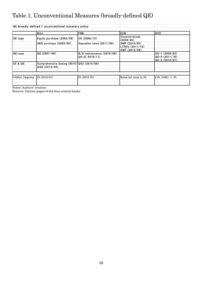
36

Table 1. Unconventional Measures (broadly-defined QE)

Notes: Authors’ creation Sources: Various pages of the four central banks

QE broadly-defined = unconventional monetary policy

BOJ FRB ECB BOE

CE-type Equity purchase (2002/09) CE (2008/12)Covered bonds(2009/06)

ABS purchase (2003/04) Operation twist (2011/09) SMP (2010/05)LTROs (2011/12)OMT (2012/09)

QE-type QE (2001-06) B/S maintenance (2010/08) QE-1 (2009/03)QE-2( 2010/11) QE-2 (2011/10)

QE-3 (2012/07)

CE & QE Comprehensive Easing (2010/ QE3 (2012/09)QQE (2013/04)

Inflation Targeting 2% (2013/01) 2% (2012/01) Below but close to 2% 2.5% (1992) -> 2%

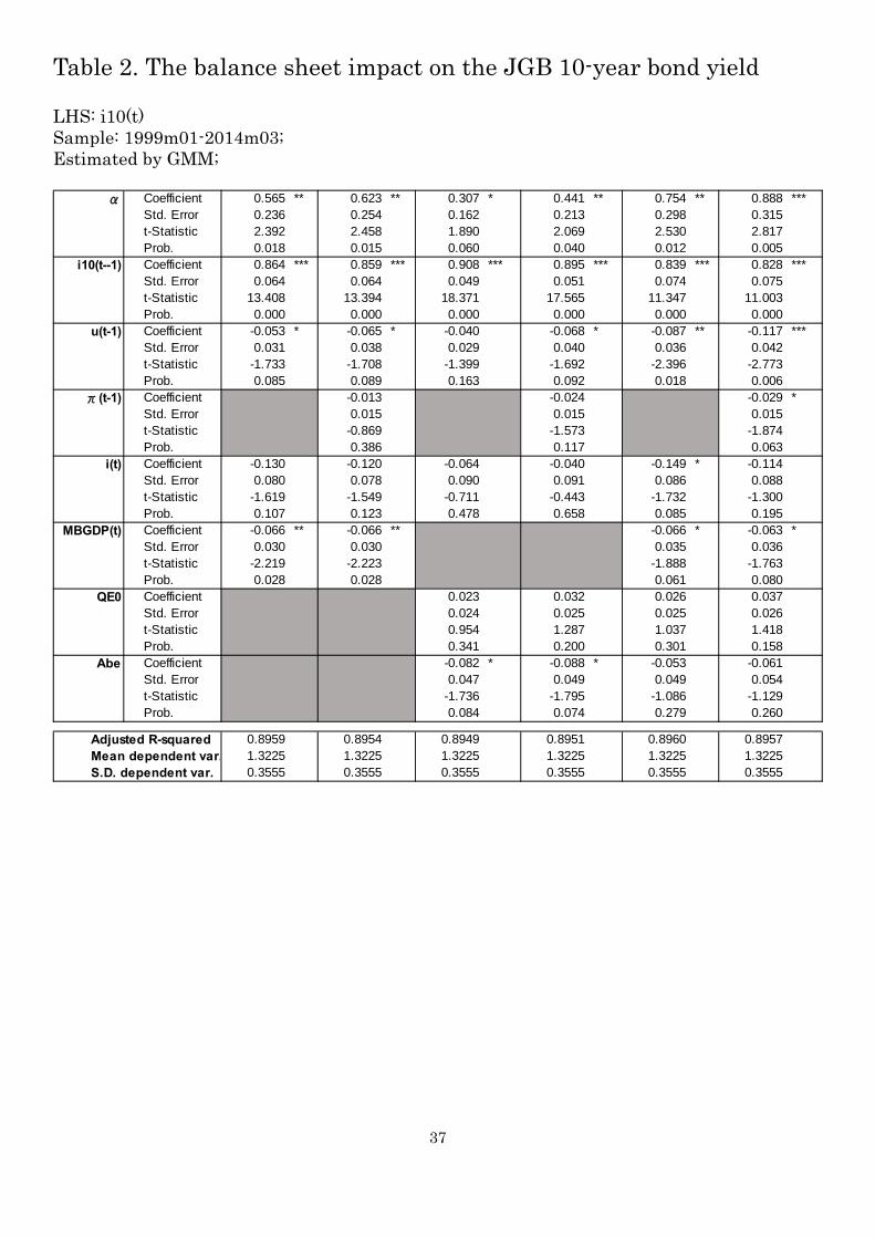
37

Table 2. The balance sheet impact on the JGB 10-year bond yield LHS: i10(t) Sample: 1999m01-2014m03; Estimated by GMM;

α Coefficient 0.565 ** 0.623 ** 0.307 * 0.441 ** 0.754 ** 0.888 ***Std. Error 0.236 0.254 0.162 0.213 0.298 0.315t-Statistic 2.392 2.458 1.890 2.069 2.530 2.817Prob. 0.018 0.015 0.060 0.040 0.012 0.005

i10(t--1) Coefficient 0.864 *** 0.859 *** 0.908 *** 0.895 *** 0.839 *** 0.828 ***Std. Error 0.064 0.064 0.049 0.051 0.074 0.075t-Statistic 13.408 13.394 18.371 17.565 11.347 11.003Prob. 0.000 0.000 0.000 0.000 0.000 0.000

u(t-1) Coefficient -0.053 * -0.065 * -0.040 -0.068 * -0.087 ** -0.117 ***Std. Error 0.031 0.038 0.029 0.040 0.036 0.042t-Statistic -1.733 -1.708 -1.399 -1.692 -2.396 -2.773Prob. 0.085 0.089 0.163 0.092 0.018 0.006

π(t-1) Coefficient -0.013 -0.024 -0.029 *Std. Error 0.015 0.015 0.015t-Statistic -0.869 -1.573 -1.874Prob. 0.386 0.117 0.063

i(t) Coefficient -0.130 -0.120 -0.064 -0.040 -0.149 * -0.114Std. Error 0.080 0.078 0.090 0.091 0.086 0.088t-Statistic -1.619 -1.549 -0.711 -0.443 -1.732 -1.300Prob. 0.107 0.123 0.478 0.658 0.085 0.195

MBGDP(t) Coefficient -0.066 ** -0.066 ** -0.066 * -0.063 *Std. Error 0.030 0.030 0.035 0.036t-Statistic -2.219 -2.223 -1.888 -1.763Prob. 0.028 0.028 0.061 0.080

QE0 Coefficient 0.023 0.032 0.026 0.037Std. Error 0.024 0.025 0.025 0.026t-Statistic 0.954 1.287 1.037 1.418Prob. 0.341 0.200 0.301 0.158

Abe Coefficient -0.082 * -0.088 * -0.053 -0.061Std. Error 0.047 0.049 0.049 0.054t-Statistic -1.736 -1.795 -1.086 -1.129Prob. 0.084 0.074 0.279 0.260

Adjusted R-squared 0.8959 0.8954 0.8949 0.8951 0.8960 0.8957Mean dependent var. 1.3225 1.3225 1.3225 1.3225 1.3225 1.3225S.D. dependent var. 0.3555 0.3555 0.3555 0.3555 0.3555 0.3555

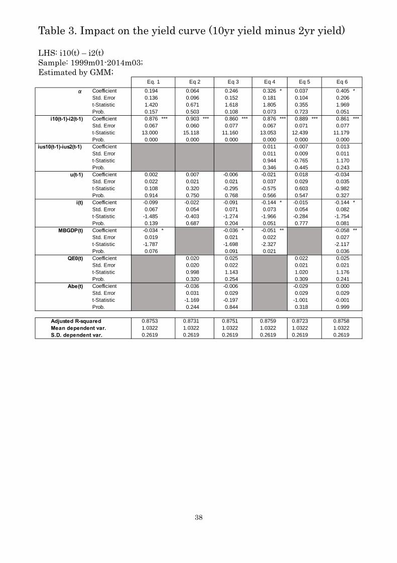
38

Table 3. Impact on the yield curve (10yr yield minus 2yr yield) LHS: i10(t) – i2(t) Sample: 1999m01-2014m03; Estimated by GMM;

α Coefficient 0.194 0.064 0.246 0.326 * 0.037 0.405 *Std. Error 0.136 0.096 0.152 0.181 0.104 0.206t-Statistic 1.420 0.671 1.618 1.805 0.355 1.969Prob. 0.157 0.503 0.108 0.073 0.723 0.051

i10(t-1)-i2(t-1) Coefficient 0.876 *** 0.903 *** 0.860 *** 0.876 *** 0.889 *** 0.861 ***Std. Error 0.067 0.060 0.077 0.067 0.071 0.077t-Statistic 13.000 15.118 11.160 13.053 12.439 11.179Prob. 0.000 0.000 0.000 0.000 0.000 0.000

ius10(t-1)-ius2(t-1) Coefficient 0.011 -0.007 0.013Std. Error 0.011 0.009 0.011t-Statistic 0.944 -0.765 1.170Prob. 0.346 0.445 0.243

u(t-1) Coefficient 0.002 0.007 -0.006 -0.021 0.018 -0.034Std. Error 0.022 0.021 0.021 0.037 0.029 0.035t-Statistic 0.108 0.320 -0.295 -0.575 0.603 -0.982Prob. 0.914 0.750 0.768 0.566 0.547 0.327

i(t) Coefficient -0.099 -0.022 -0.091 -0.144 * -0.015 -0.144 *Std. Error 0.067 0.054 0.071 0.073 0.054 0.082t-Statistic -1.485 -0.403 -1.274 -1.966 -0.284 -1.754Prob. 0.139 0.687 0.204 0.051 0.777 0.081

MBGDP(t) Coefficient -0.034 * -0.036 * -0.051 ** -0.058 **Std. Error 0.019 0.021 0.022 0.027t-Statistic -1.787 -1.698 -2.327 -2.117Prob. 0.076 0.091 0.021 0.036

QE0(t) Coefficient 0.020 0.025 0.022 0.025Std. Error 0.020 0.022 0.021 0.021t-Statistic 0.998 1.143 1.020 1.176Prob. 0.320 0.254 0.309 0.241

Abe(t) Coefficient -0.036 -0.006 -0.029 0.000Std. Error 0.031 0.029 0.029 0.029t-Statistic -1.169 -0.197 -1.001 -0.001Prob. 0.244 0.844 0.318 0.999

Adjusted R-squared 0.8753 0.8731 0.8751 0.8759 0.8723 0.8758Mean dependent var. 1.0322 1.0322 1.0322 1.0322 1.0322 1.0322S.D. dependent var. 0.2619 0.2619 0.2619 0.2619 0.2619 0.2619

Eq 6Eq. 1 Eq 2 Eq 3 Eq 4 Eq 5

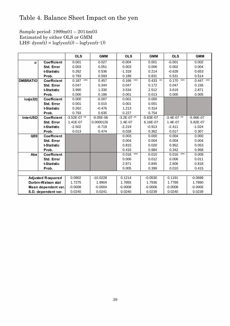
39

Table 4. Balance Sheet Impact on the yen Sample period: 1999m01 – 2014m03 Estimated by either OLS or GMM LHS: dyen(t) = log(yen(t)) – log(yen(t-1))

OLS GMM OLS GMM OLS GMM

α Coefficient 0.001 0.027 -0.004 0.001 -0.001 0.002Std. Error 0.003 0.051 0.003 0.006 0.002 0.004t-Statistic 0.262 0.536 -1.318 0.214 -0.628 0.653Prob. 0.793 0.593 0.189 0.831 0.531 0.514

DMBRATIO Coefficient 0.187 *** 0.457 0.166 *** 0.433 ** 0.170 *** 0.447 ***Std. Error 0.047 0.344 0.047 0.172 0.047 0.156t-Statistic 3.990 1.330 3.534 2.512 3.619 2.871Prob. 0.000 0.186 0.001 0.013 0.000 0.005

iusja2(t) Coefficient 0.000 -0.007 0.001 0.000Std. Error 0.001 0.015 0.001 0.001t-Statistic 0.262 -0.476 1.213 0.314Prob. 0.793 0.635 0.227 0.754

InterUSD Coefficient -3.52E-07 ** -9.05E-06 -3.2E-07 ** -5.63E-07 -3.4E-07 ** -5.96E-07Std. Error 1.41E-07 0.0000126 1.4E-07 6.16E-07 1.4E-07 5.82E-07t-Statistic -2.502 -0.719 -2.219 -0.913 -2.411 -1.024Prob. 0.013 0.474 0.028 0.362 0.017 0.307

QE0 Coefficient 0.003 0.000 0.004 0.000Std. Error 0.004 0.004 0.004 0.004t-Statistic 0.815 0.020 0.952 0.053Prob. 0.416 0.984 0.342 0.958

Abe Coefficient 0.018 *** 0.010 0.016 *** 0.009Std. Error 0.006 0.012 0.006 0.011t-Statistic 2.871 0.845 2.606 0.818Prob. 0.005 0.399 0.010 0.415

Adjusted R-squared 0.0902 -10.0228 0.1214 -0.0530 0.1191 -0.0698Durbin-Watson stat 1.7275 1.9904 1.7855 1.7936 1.7789 1.7890Mean dependent var. -0.0008 -0.0004 -0.0008 -0.0006 -0.0008 -0.0006S.D. dependent var. 0.0240 0.0241 0.0240 0.0239 0.0240 0.0239

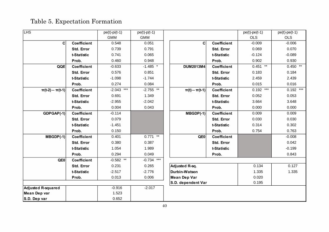
40

Table 5. Expectation Formation

LHS pe(t)-pi(t-1) pe(t)-p(t-1) pe(t)-pe(t-1) pe(t)-pe(t-1)GMM GMM OLS OLS

C Coefficient 0.548 0.051 C Coefficient -0.009 -0.006

Std. Error 0.739 0.791 Std. Error 0.069 0.070

t-Statistic 0.741 0.065 t-Statistic -0.124 -0.089

Prob. 0.460 0.948 Prob. 0.902 0.930

QQE Coefficient -0.633 -1.485 * DUM2013M4 Coefficient 0.451 ** 0.450 **

Std. Error 0.576 0.851 Std. Error 0.183 0.184

t-Statistic -1.098 -1.744 t-Statistic 2.459 2.439

Prob. 0.274 0.084 Prob. 0.015 0.016

π(t-2)－π(t-1) Coefficient -2.043 *** -2.755 ** π(t)－π(t-1) Coefficient 0.192 *** 0.192 ***

Std. Error 0.691 1.349 Std. Error 0.052 0.053

t-Statistic -2.955 -2.042 t-Statistic 3.664 3.648

Prob. 0.004 0.043 Prob. 0.000 0.000

GDPGAP(-1) Coefficient -0.114 MBGDP(-1) Coefficient 0.009 0.009

Std. Error 0.079 Std. Error 0.030 0.030

t-Statistic -1.451 t-Statistic 0.314 0.302

Prob. 0.150 Prob. 0.754 0.763

MBGDP(-1) Coefficient 0.401 0.771 ** QE0 Coefficient -0.008

Std. Error 0.380 0.387 Std. Error 0.042

t-Statistic 1.054 1.989 t-Statistic -0.199

Prob. 0.294 0.049 Prob. 0.843

QE0 Coefficient -0.582 ** -0.734 ***

Std. Error 0.231 0.265 Adjusted R-sq. 0.134 0.127

t-Statistic -2.517 -2.776 Durbin-Watson 1.335 1.335

Prob. 0.013 0.006 Mean Dep Var 0.020

S.D. dependent Var 0.195

Adjusted R-squared -0.916 -2.017

Mean Dep var 1.523

S.D. Dep var 0.652

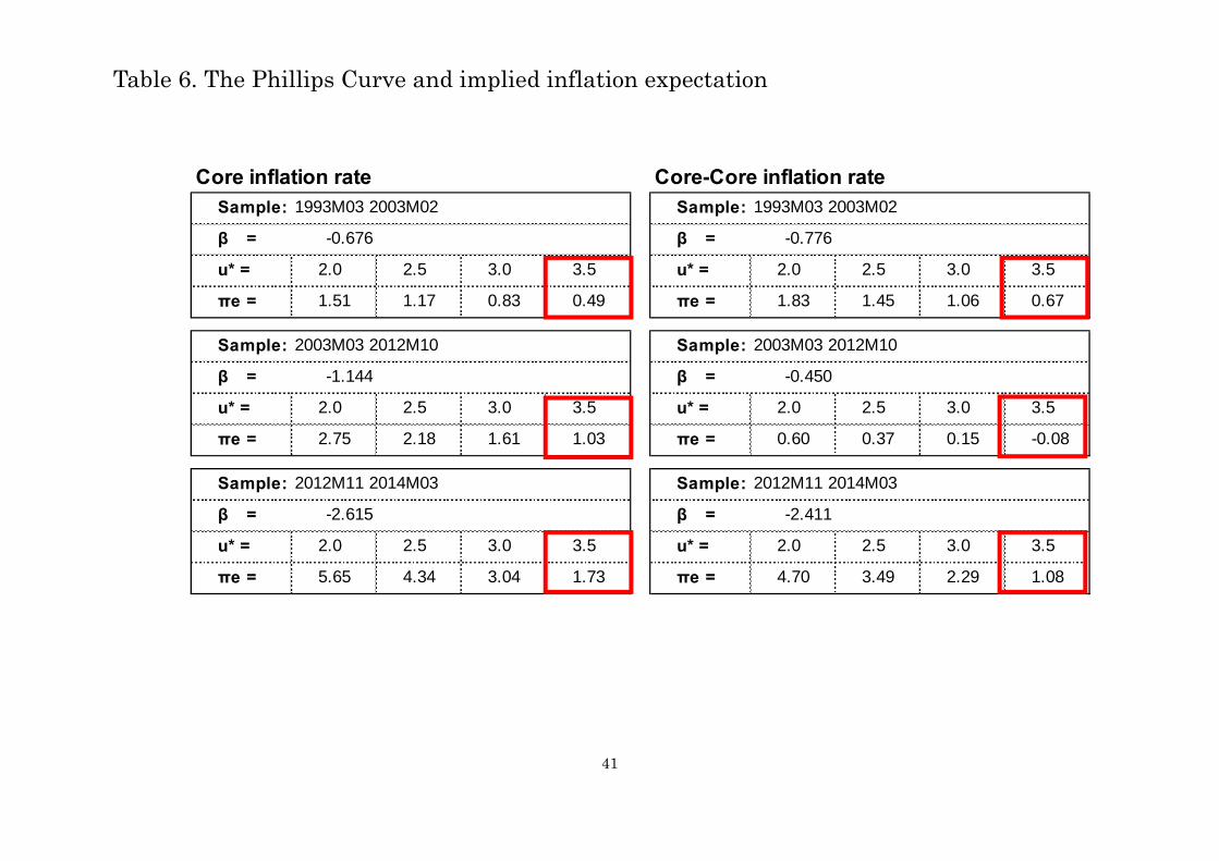
41

Table 6. The Phillips Curve and implied inflation expectation

Core inflation rate Core-Core inflation rateSample: 1993M03 2003M02 Sample: 1993M03 2003M02

β　= -0.676 β　= -0.776

u* = 2.0 2.5 3.0 3.5 u* = 2.0 2.5 3.0 3.5

πe = 1.51 1.17 0.83 0.49 πe = 1.83 1.45 1.06 0.67

Sample: 2003M03 2012M10 Sample: 2003M03 2012M10

β　= -1.144 β　= -0.450

u* = 2.0 2.5 3.0 3.5 u* = 2.0 2.5 3.0 3.5

πe = 2.75 2.18 1.61 1.03 πe = 0.60 0.37 0.15 -0.08

Sample: 2012M11 2014M03 Sample: 2012M11 2014M03

β　= -2.615 β　= -2.411

u* = 2.0 2.5 3.0 3.5 u* = 2.0 2.5 3.0 3.5

πe = 5.65 4.34 3.04 1.73 πe = 4.70 3.49 2.29 1.08

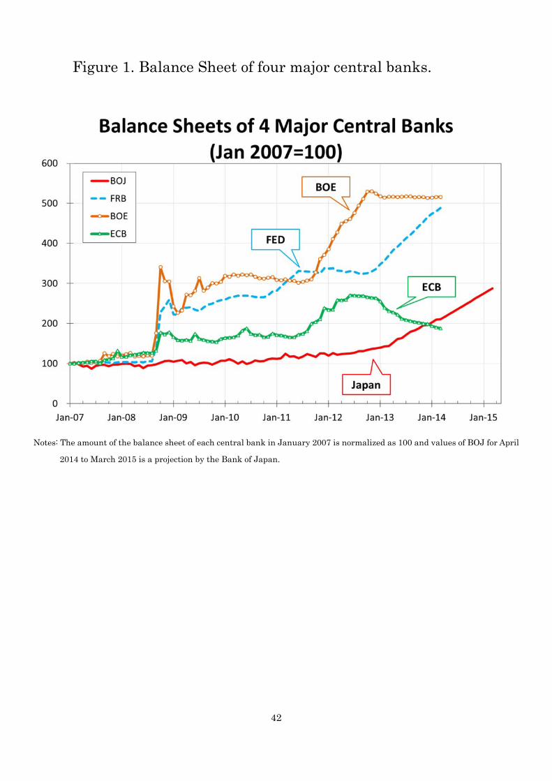
42

Figure 1. Balance Sheet of four major central banks.

Notes: The amount of the balance sheet of each central bank in January 2007 is normalized as 100 and values of BOJ for April

2014 to March 2015 is a projection by the Bank of Japan.

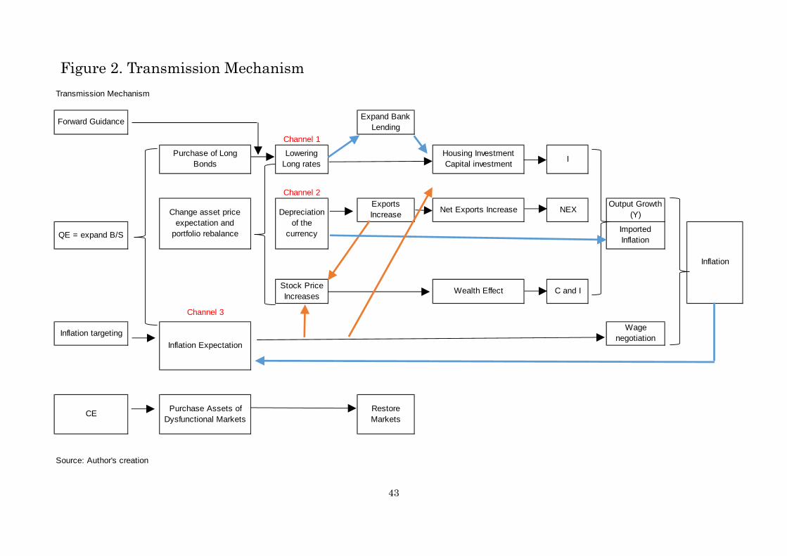
43

Figure 2. Transmission Mechanism

Transmission Mechanism

Forward GuidanceExpand Bank

Lending

Channel 1

Purchase of LongBonds

LoweringLong rates

Housing InvestmentCapital investment

I

Channel 2ExportsIncrease

Net Exports Increase NEXOutput Growth

(Y)

QE = expand B/SImportedInflation

Stock PriceIncreases

Wealth Effect C and I

Channel 3

Inflation targetingWage

negotiation

CEPurchase Assets of

Dysfunctional MarketsRestoreMarkets

Source: Author's creation

Inflation Expectation

Depreciationof the

currency

Change asset priceexpectation and

portfolio rebalance

Inflation

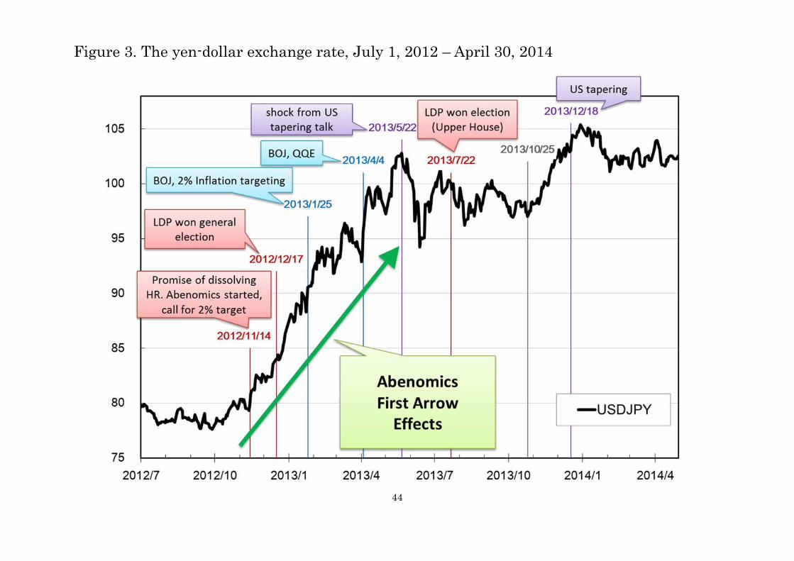
44

Figure 3. The yen-dollar exchange rate, July 1, 2012 – April 30, 2014

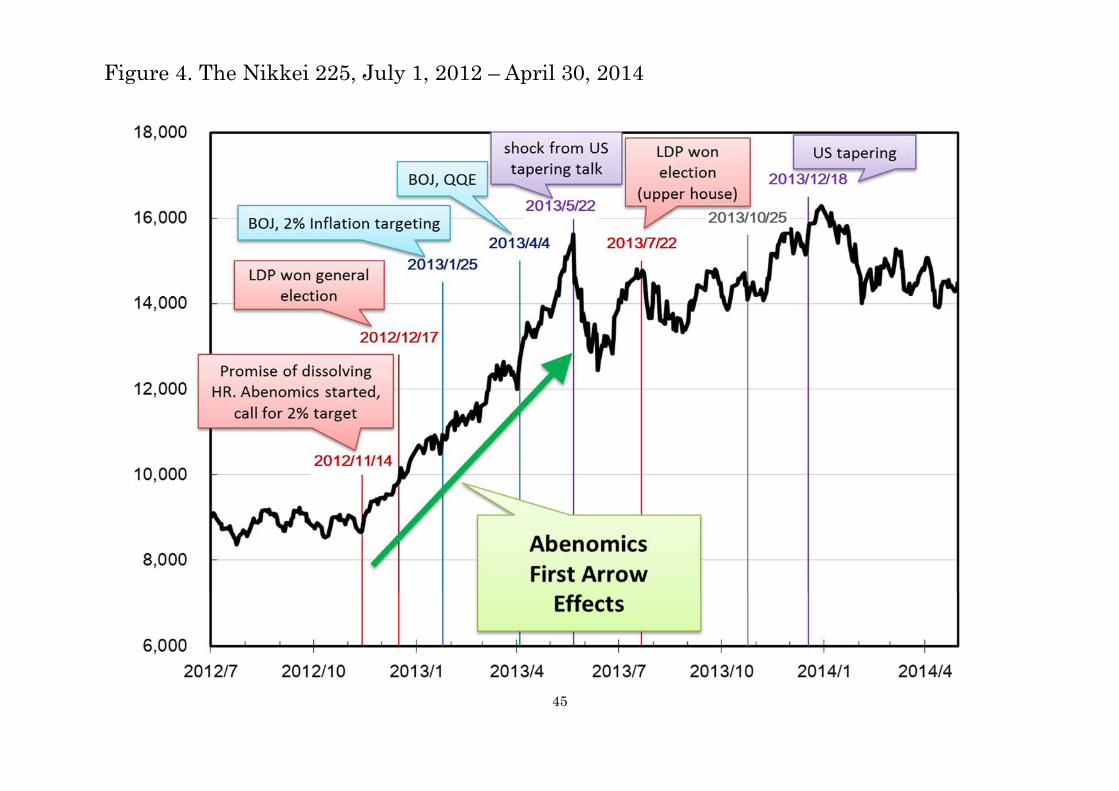
45

Figure 4. The Nikkei 225, July 1, 2012 – April 30, 2014

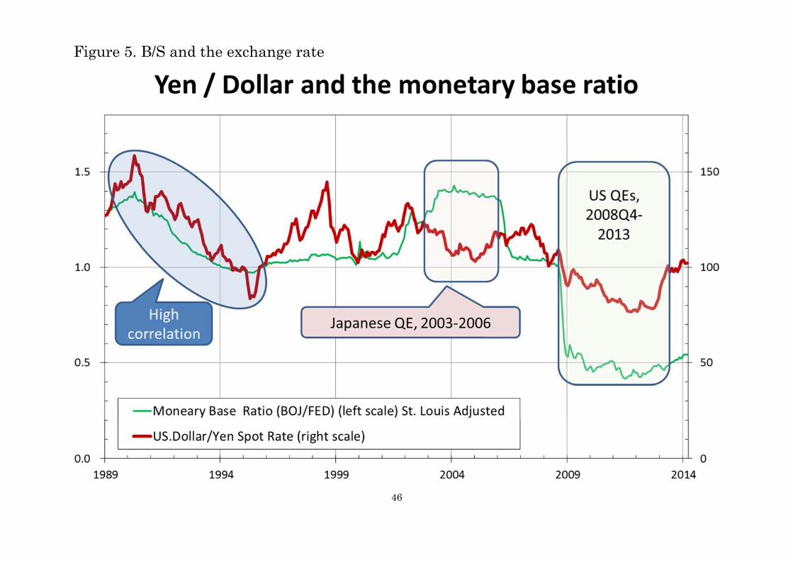
46

Figure 5. B/S and the exchange rate

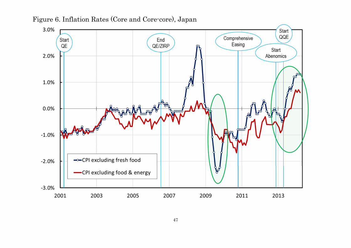
47

Figure 6. Inflation Rates (Core and Core-core), Japan

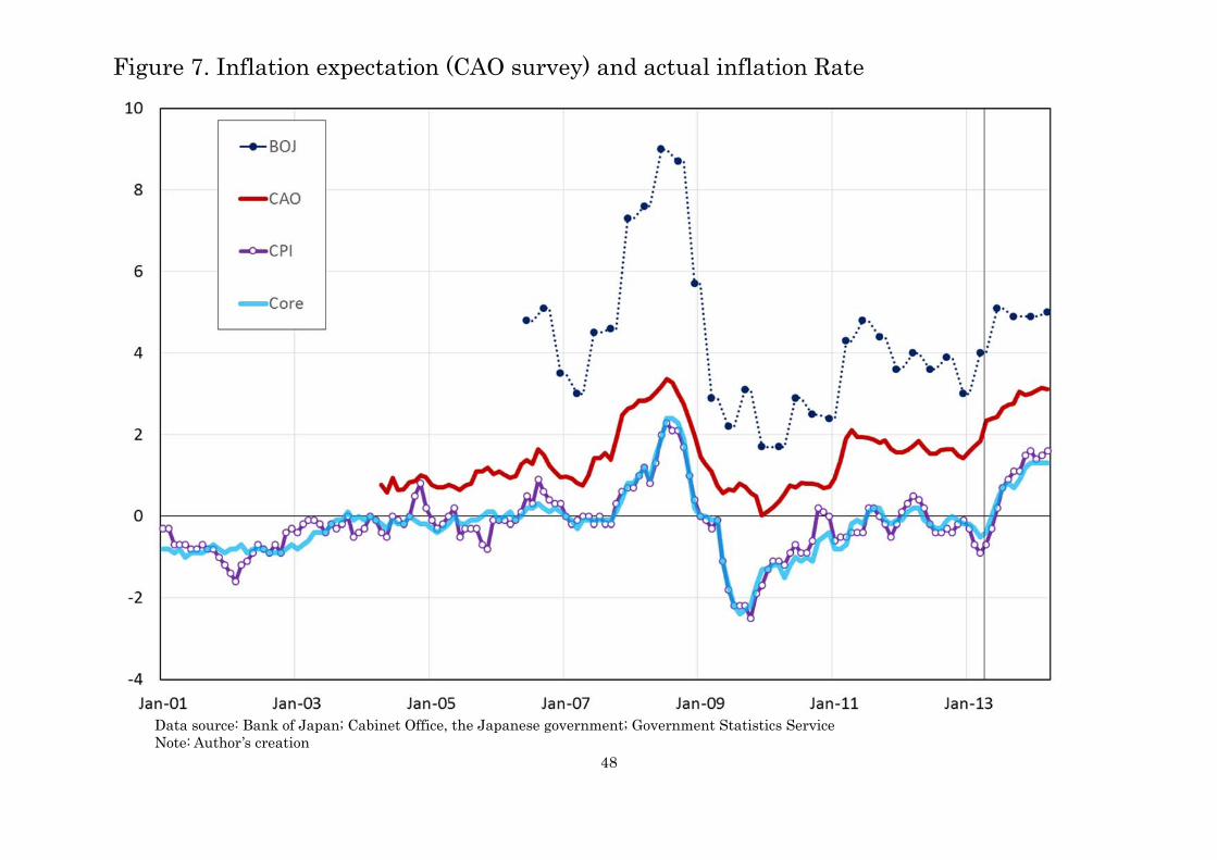
48

Figure 7. Inflation expectation (CAO survey) and actual inflation Rate

Data source: Bank of Japan; Cabinet Office, the Japanese government; Government Statistics Service Note: Author’s creation

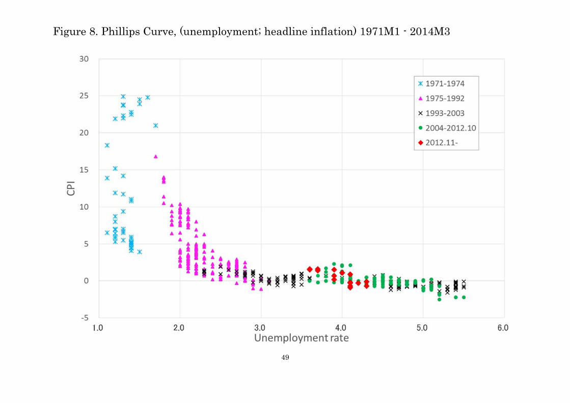
49

Figure 8. Phillips Curve, (unemployment; headline inflation) 1971M1 - 2014M3

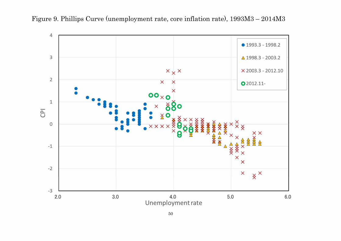
50

Figure 9. Phillips Curve (unemployment rate, core inflation rate), 1993M3 – 2014M3

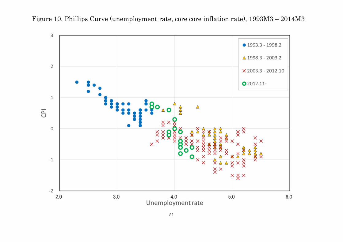
51

Figure 10. Phillips Curve (unemployment rate, core core inflation rate), 1993M3 – 2014M3