TAG UNIT M1

Principles of Modelling and Forecasting

January 2014

Department for Transport

Transport Analysis Guidance (TAG)

https://www.gov.uk/transport-analysis-guidance-tag

This TAG Unit is guidance for the MODELLING PRACTITIONER

This TAG Unit is part of the family M1 – MODELLING PRINCIPLES

Technical queries and comments on this TAG Unit should be referred to:

Transport Appraisal and Strategic Modelling (TASM) Division Department for Transport Zone 2/25 Great Minster House 33 Horseferry Road London SW1P 4DR tasm@dft.gov.uk

Contents

1 Introduction 1

1.1 Scope of this unit 1 1.2 Structure of this unit 1

2 Rationale for Forecasting and Modelling 1

2.1 Demand Units for Transport Schemes 1 2.2 Forecasting 2 2.3 Modelling 3 2.4 Priorities 4

3 Data collection 4

4 Modelling 5

4.1 Introduction 5 4.2 The Standard Model Structure 5 4.3 The Demand Model 8 4.4 The Assignment Model 11 4.5 Interfaces between Demand and Assignment models 12 4.6 Alternative Model Structures 12 4.7 Mitigating Modelling Risks 14

5 Forecasting 15

5.1 Introduction 15 5.2 Forecast Design 15 5.3 Mitigating Forecasting Risks 15

6 References 17

7 Document Provenance 17

TAG Unit M1.1

Principles of Modelling and Forecasting

1 Introduction

1.1 Scope of this unit

1.1.1 Transport provision is often updated to improve users’ experience (for example, reducing journey

time or improving comfort) or to address problems created by transport infrastructure (such as

negative environmental or safety impacts). Decisions will need to be made regarding whether to

make changes to the network, and which option for change should be implemented. These

decisions should be informed by evidence of existing or anticipated future problems that have been

identified, the effectiveness of viable options in addressing them, and also the consequences of

implementing each option. Evidence should be of adequate quality to make decisions, compiled

using proportionate resources.

1.1.2 All evidence needs to be based on a set of assumptions about the future (or forecast), but not all

impacts of transport interventions have an accepted method for quantifying or monetising them.

Quantifiable impacts are usually forecasted using a suitable model.

1.1.3 The modelling and forecasting guidance in TAG exists to enable practitioners to produce adequate

evidence to support the business case for major transport schemes. It may be useful for other

purposes, but it is not a comprehensive textbook on modelling practice. Assessment of smaller

schemes may make proportionate use of parts of the guidance or use simpler methods in proportion

with the size of the scheme (e.g. a detailed model of a single junction rather than a larger model of a

transport network).

1.1.4 This unit exists to help modelling and forecasting practitioners understand why modelling and

forecasting are required, and the principles behind the Department’s approach. Step-by-step

guidance, along with the standards and tolerances the Department expects, are given in TAG Units

M2 – Variable Demand Modelling, M3.1 – Highway Assignment Modelling, M3.2 – Public Transport

Assignment Modelling and M4 – Forecasting and Uncertainty.

1.2 Structure of this unit

1.2.1 Section 2 explains why forecasting and (usually) modelling and data collection are required to

produce evidence for decision makers regarding transport schemes. Later sections explain the

principles behind why the approach set out in TAG guidance is recommended with regard to:

• data collection (section 3);

• modelling (section 4);

• forecasting (section 5).

2 Rationale for Forecasting and Modelling

2.1 Demand Units for Transport Schemes

2.1.1 In order to quantify the impacts of any intervention (transport or otherwise), it is necessary to define

a unit of consumption. The number of units (demand) and cost per unit (supply) can then be

calculated and compared for different options.

2.1.2 Transport systems enable consumers to travel between two locations. The impact of transport

systems can be measured using units of trips. A trip is a one-way course of travel between two

locations for a given purpose.

2.1.3 However, transport has other impacts (including noise, air quality, and accidents) which depend on

the location of the infrastructure and the extent to which it is used. These are often assessed using

vehicle flows , either for highway or public transport. Some impacts also require information on the

Page 1

TAG Unit M1.1

Principles of Modelling and Forecasting

number and size of households (and details of other buildings where transport may have a

significant effect, such as schools or hospitals) located close to the infrastructure.

2.1.4 These units need to be estimated for future years, using forecasts prepared with an appropriate

model.

2.2 Forecasting

2.2.1 Assessment of any intervention (transport or otherwise) requires an appreciation of expected future

benefits and disbenefits. Being in the future, these benefits and disbenefits cannot be measured or

observed at the time the decision needs to be made, and so they need to be estimated by

comparing two forecasts – one excluding the intervention, the other including the intervention and

no other changes.

2.2.2 In the transport context, these two forecasts are called the without-scheme forecast and with-

scheme forecast respectively. Often, separate pairs of forecasts are required for at least two

forecast years, to take into account changes in population and other transport infrastructure over

time. TAG Unit A1.1 – Cost Benefit Analysis gives more guidance on selecting forecast years.

2.2.3 Each forecast relies heavily on assumptions about:

• the number of potential users;

• the behaviour of the users;

• the cost of using the infrastructure, which is related to the infrastructure provision.

2.2.4 These can be represented using the economic concepts of demand (covering the number of users

and their behaviour in response to infrastructure provision) and supply (the cost of using the

infrastructure).

2.2.5 In order for forecasts to be credible, the assumptions need to be realistic. Also, as different transport

schemes often compete for a common budget, it is important that the forecasting assumptions are

consistent and unbiased so that the budget can be allocated on a fair basis.

2.2.6 For some assumptions (for example population growth), future projections are published by other

Government departments. These may be sufficient to analyse demand for some public services (not

transport), based on the population changes within a given catchment area.

2.2.7 Transport, however, has a more complex spatial structure. Demand for transport is based not on

individual locations but on interactions between pairs of locations, and the location and layout of

infrastructure connecting them. Whilst population and economic projections are useful for estimating

total travel demand from or to a given location, they cannot inform how users will choose to travel

between pairs of locations, and consequently a forecasting model is required, as discussed in

section 2.3.

2.2.8 The main basis for appraisal of major transport schemes should be the core scenario, based on

unbiased and realistic assumptions. TAG Unit M4 – Forecasting and Uncertainty gives guidance

about preparing this scenario.

2.2.9 Forecasts are, by nature, uncertain. Even when using unbiased assumptions (as in the core

scenario) there is no guarantee that the outturn result of the implementing the scheme will match the

forecast. It is also not sufficient to use a “worst case scenario”, or a lower or upper bound, as there

are risks associated with both lower and higher levels of demand or supply than forecast.

2.2.10 Modifications to the transport network should therefore be tested under different assumptions

(compiled as alternative scenarios) to highlight any risks to the benefits or impacts. of the scheme.

Page 2

TAG Unit M1.1

Principles of Modelling and Forecasting

Alternative scenarios should cover any significant sources of uncertainty, but their use should be

proportionate.

2.3 Modelling

2.3.1 A transport model is a tool (usually an automated computer program) that converts readily available

forecasting assumptions into a forecast of demand (number of trips) and supply (level of service /

cost of travel) on the transport network. Transport models are therefore constrained by the

availability of forecasting data, technical expertise and resources on one side and the appraisal

outputs required on the other.

2.3.2 Models themselves are underpinned by a large number of assumptions, including:

• that the structure of the model (which should be based on economic principles) is a sound

representation of human behaviour;

• that any necessary simplifications within the model, including the representation of the network,

the segmentation of the population by person type, and the segmentation of the spatial area, do

not have a material effect in forecasting the results, and

• the numerical parameters used in the model, many of which cannot be observed directly and

therefore need to be estimated using a sample of data and statistical principles (a process known

as calibration).

2.3.3 Before using models for analytical work, the analyst should specify the capabilities required from the

model and the assumptions that would be deemed acceptable. In some circumstances cost savings

may be achieved by using an existing model, but a model constructed for one project cannot

necessarily be used for another, even if it covers the correct geographical area. The analytical

approach needs to be defined from the start of the project; failure to do so may lead to analysis

needing to be repeated, adding to the cost.

2.3.4 There is a risk that model may not be realistic or sensible due to the error around the model

parameters used, or limitations in the extent to which the model can represent human behaviour.

Therefore, before using any mathematical model, it is essential to check that it produces credible

outputs consistent with observed behaviour. This is usually done by running the model for the base

year (either the current year or a recent year), and:

• comparing its outputs with independent data (validation);

• checking that its response to changes in inputs is realistic, based on results from independent

evidence (realism testing); and

• checking that the model responds appropriately to all its main inputs (sensitivity testing).

2.3.5 Both the calibration and validation processes described above can create a requirement for

bespoke data collection, discussed in section 3.

2.3.6 Transport models can take a long time to run and generate a large quantity of data, and even the

best models are imperfect representations of reality. Therefore, the construction and use of models

should be proportionate, and analysts who prepare models should be aware of their limitations,

and communicate the risks that such limitations create. Given the limits of resources available for

modelling, analysts should consider the trade-off between developing the model (in terms of its

accuracy and functionality) and carrying out additional forecasting work to test for sensitivity and

uncertainty.

Page 3

TAG Unit M1.1

Principles of Modelling and Forecasting

2.4 Priorities

2.4.1 It can be seen that:

• the quality of evidence depends primarily on the quality of the forecasts used to underpin it and

communication about the known risks of using these forecasts; and

• the quality of forecasts, in turn, relies on the quality of any models being used and a good

understanding of their limitations.

2.4.2 The priority for the transport modelling practitioner, therefore, should be to produce forecasts of

adequate quality using proportionate resources. It is likely that modelling will be required for this

purpose, and TAG gives guidance on the acceptability guidelines expected of models for the

purpose of appraising major transport schemes.

2.4.3 It should be emphasised that it may not be necessary to use the most sophisticated or detailed

models, nor is it likely to be appropriate to invest the highest proportion of resources to develop the

best quality model at the expense of interpreting its outputs carefully and communicating its

limitations.

3 Data collection

Note: this section only introduces data collection for the purpose of calibrating and validating

models. The collection of forecasting data is described in TAG Unit M4 – Forecasting and

Uncertainty.

3.1.1 Data collection is necessary in order to inform the parameters that represent the model responses

(calibration) and to provide a source of information against which the model can be compared to

assure its quality (validation).

3.1.2 The main constraints on data collection for modelling are:

• which data are available, and the cost of collecting it; and

• which data are useful to inform the calibration and validation of the model.

3.1.3 Five types of data can be collected and used to inform most models:

• data on the transport network, including the physical layout, number of lanes, signal timings,

public transport frequencies and capacities;

• counts of vehicles or persons on transport services, links or at junctions;

• journey times;

• queue lengths at busy junctions;

• interview surveys, in which transport users are asked to describe trips either through household

travel diaries or intercept surveys (e.g. roadside interviews, public transport onboard interview

surveys.

3.1.4 The first four of these can be collected without interviewing, and consequently they typically yield a

large quantity of data at relatively little cost. However, they do not provide details of travellers’ origin and destination, nor their reason for travel (trip purpose). Traditionally, this information has been

collected using interview surveys. Increasingly, automated non-interview methods of collecting

origin-destination data (such as automated number-plate recognition and data from electronic

devices) are becoming available. Analysts who use such data should be aware of its limitations (e.g.

Page 4

TAG Unit M1.1

Principles of Modelling and Forecasting

it may not always be able to segment trips by purpose, and there may be additional sources of bias

that would not exist in interview surveys).

3.1.5 There are many risks with collecting and interpreting data samples. These should be mitigated by:

• ensuring that samples are of adequate quality and sufficiently large;

• recognising the statistical limitations of the sample (for example the scale of sample error); and

• collecting data under typical conditions (e.g. not during holiday periods or at times of extreme

weather). Sometimes data collection needs to be repeated if an unforeseen event occurs (such

as an accident or adverse weather) and the resultant data is distorted.

3.1.6 Data collection is usually the most resource-intensive aspect of transport modelling. It is therefore

highly advisable to minimise the amount of data that needs to be collected, by:

• taking into account data requirements in the design of the model; and

• using data that has already been collected, where this is of adequate quality.

3.1.7 At the same time, it should be noted that minimising data collection can increase the risks of

calibrating and validating the model.

3.1.8 More detailed guidance on data collection is given in TAG Unit M1.2 – Data Sources and Surveys.

4 Modelling

4.1 Introduction

4.1.1 The quality of the forecast depends on the quality of any underlying models. Over a number of years

a standard structure has been developed for modelling transport demand and supply, based on

economic principles. Sections 4.2 to 4.5 describe this standard structure, whilst Appendix A explains

the principles.

4.1.2 Other structures exist, but the standard structure is usually adequate and the most proportionate for

modelling major schemes. Section 4.6 briefly describes some alternative structures for transport

models. The Department welcomes innovation and practitioners may make a case to the

Department for using different structures, providing they produce adequate evidence and do not

require disproportionate resources.

4.1.3 Even models based on sound economic theory may not represent human behaviour adequately

well, and this is a risk to the quality of the forecasts. Therefore it is important to establish the

credibility of models in practice as well as in theory. Section 4.7 discusses how this, and other

modelling risks, should be mitigated.

4.2 The Standard Model Structure

4.2.1 Figure 1, on the next page, shows the standard model structure in a flow chart format.

Page 5

TAG Unit M1.1

Principles of Modelling and Forecasting

Demand Model

Link Demand

TRIP DEMAND (matrix)

TRIP COST (matrix)

Cost Parameters

Trip End Model

Evidence

Network layout

Demographic data

Route cost

Link cost

Route Choice

Network capacity

ASSIGNMENT MODEL

Key to box and arrow styles

Main loop (variable demand model)

Inner loop (assignment model)

Forecasting inputs

Appraisal

Figure 1 The standard transport model structure

4.2.2 Economic analysis of transport is usually based on units of trips. Transport models calculate

forecasts of the following quantities given assumptions about the transport network and travel

demand:

• the number of trips (demand);); and

• the cost of each trip (supply).

Page 6

TAG Unit M1.1

Principles of Modelling and Forecasting

4.2.3 These quantities need to be segmented by origin, destination, time period and mode. This is

handled by storing both demand and supply in multi-dimensional arrays, known as the trip matrix

and the cost matrix respectively.

4.2.4 The costs of travel take many forms, including travel time and financial cost, but a single measure of

cost will usually be required in order to calculate the trip matrix. Therefore, the various costs of travel

are often combined into a generalised cost, usually a linear combination of each cost component,

which reflects overall perception of difficulty of travel.

4.2.5 Except in the very smallest models, it is not usually practical to model trips to or from each individual

house, workplace or shop. Accordingly, spatial areas are usually aggregated to zones, and the trip

matrix and the cost matrix are usually segmented by pairs of zones. It may not always be necessary

to use the same zoning system for supply and demand, providing appropriate interfaces can be

made between the zoning systems. Further guidance on defining zones is given in TAG Unit M2 – Variable Demand Modelling and TAG Unit M3.1 – Highway Assignment Modelling.

4.2.6 The demand model (see section 4.3) is used to forecast the trip matrix, based on:

• the most up-to-date estimate of the cost matrices; and

• a measure of travel demand based on the demographic data assumptions (population and

employment). The measure most commonly used is known as trip ends, and these are

calculated using a trip end model.

4.2.7 For appraising major transport schemes, the Department strongly prefers the use of incremental

demand models in preference to absolute models. Incremental models update a trip matrix heavily

based on observed data for the base year, whereas absolute models calculate the trip matrix for

each forecast year directly based on trip ends and costs. Incremental models rely more on observed

data less on the mathematical specification of the model than absolute models.

4.2.8 When using a fixed demand approach, as discussed in section 4.3, it will not be necessary to have a

cost-dependent demand model, but trip ends will still be used to implement the effects of changes in

demographic data between forecast years.

4.2.9 The cost matrix is calculated using the assignment model (section 4.4) which is based on:

• the most up-to-date estimate of the trip matrix; and

• a network model (a mathematical representation of the transport network), which is used to

calculate the cost of travel between each pair of zones.

4.2.10 Assignment models have a dual role – as well as calculating the cost matrix, they also allocate the

trips by route and calculate demand for each link in the network. This supports analysis of the

impacts of transport infrastructure, which is particularly important for highways.

4.2.11 In general, the demand model and assignment model depend on each other. In order to provide a

systematic basis to compare forecasts, they should be run alternately until they have converged to

equilibrium within specified tolerances (discussed further in Appendix A). This creates the need for a

loop structure, which requires much greater run times than would otherwise be the case.

4.2.12 A further demand-supply loop is required within the assignment model itself. The assignment model

calculates both the demand and cost for individual links and junctions in the network. The demand

and cost depend on each other as follows:

• the demand for each link depends on the number of trips between each pair of zones (from the

trip matrix) and the routes they choose (which are dependent on the cost of choosing each

route); and

Page 7

Overview

TAG Unit M1.1

Principles of Modelling and Forecasting

• the cost (in particular, the travel time) of travelling along each link or junction depends on its

demand and the mathematical relationship between demand, capacity and cost. These

mathematical relationships are defined in the network model.

4.3 The Demand Model

4.3.1 The demand model forecasts trip matrices based on:

• trip ends; and

• travel costs, and assumptions about travellers’ behavioural response to cost (in most cases).

4.3.2 There are a wide range of principles relating to the modelling of travel demand, each of which is

discussed under a separate header below:

• segmentation of the model, particularly by trip purpose and person type

• representation of the trip pattern, taking into account how series of individual trips are made by

transport users;

• representation of travellers’ response to cost;

• whether the model generates a new trip matrix solely from trip ends and costs (an absolute

model) or updates an existing matrix (incremental); and

• which behavioural responses to include, and which model to use for each response.

Segmentation of the model

4.3.3 Travel behaviour often varies also by trip purpose and person type characteristics including age,

the extent to which the person is working, household structure, and household car ownership. In

general, separate demand models will need to be developed for the following three trip purposes, as

they have different parameters:

• Employers’ business;

• Commuting (to work);

• Other.

4.3.4 Increasing the number of trip purposes, or using a large number of person types, can improve the

capability of the model but will increase its complexity and cost; the cost of data collection may also

be increased. Consideration might be given to using greater segmentation for those parts of the

calculation that are least data-hungry (particularly person type segmentation in trip end models).

Representation of the trip pattern

4.3.5 Demographic data (e.g. population and employment data) is specific to a single zone. This means it

does not form a good indicator of the quantity of travel between a pair of zones, but it can inform

total demand to and from each zone, or trip ends.

4.3.6 Trip ends are the format in which the Department provides its standard forecasts of growth in

demand. They can be calculated quite simply by multiplying demographic data by trip rates, which

can be estimated from survey data. Most models will have a trip end model to handle planned local

changes in housing and employment data. When forecasting, however, growth in trip ends should

be controlled to growth factors from the NTEM dataset at a suitably aggregate spatial level. The

method for doing this is given in TAG Unit M4 – Forecasting and Uncertainty.

Page 8

TAG Unit M1.1

Principles of Modelling and Forecasting

4.3.7 Although individual trips are used as the unit of travel demand, transport users do not make a single

trip in isolation, but instead undertake a series of trips in order to carry out one or more activities. A

series of trips undertaken between leaving home and returning home is commonly called a tour.

4.3.8 In most models, it is convenient to split trips according to their position in the tour – whether

outbound from home, return to home, or non-home-based trips – and to define the trip ends by

production (the location where the decision to travel is made) and attraction (the reason for travel).

The production / attraction (P/A) definition of trip ends is explained further in Appendix B – it can

differ from the origin / destination (O/D) definition, in which the trip ends are characterised by the

beginning (origin) and end (destination) of the trip.

Representation of travellers’ response to cost

4.3.9 There are three broad approaches to representing travellers’ response to cost:

• a fixed demand approach, in which demand is independent of cost, and the trip matrix is

adjusted using trip ends and no behavioural model is required;

• an own cost elasticity approach where demand in each cell of the trip matrix can vary, but the

source of any variation is limited to the corresponding cell of the cost matrix only; or

• a full variable demand approach where demand in each cell of the matrix can vary according to

demand in other cells of the trip matrix and costs in all cells of the cost matrix. This is usually

implemented using discrete choice models, which are described from paragraph 4.3.13 below.

4.3.10 Fixed demand approaches have the quickest run times as they do not require the demand and

assignment models to be run alternately. However, their use is only valid where it can be

demonstrated that changes in cost will not generate a noticeable change in demand (commonly

called induced traffic). As such, fixed demand models are inadequate for most transport schemes

which are aimed at resolving congestion or relieving overcrowding on public transport.

4.3.11 Own-cost elasticity models do not constrain total demand according to the size of the population.

This means they are not adequate for representing either the transport market as a whole, or modes

with a high share of overall travel, such as car. However, they have advantages over choice models

when analysing rail schemes:

• own cost elasticity models are less expensive to build and run;

• rail schemes often cover a large spatial area, and it is difficult and expensive to collect the

quantity of data that would be required for a variable demand choice model; and

• they are more consistent with observed demand.

4.3.12 Variable demand models assume that (travel costs notwithstanding) the trip rate for any given

demographic segment is constant through time. The National Travel Survey (NTS) supports the

validity of this assumption in terms of total trip rates, which are strongly dominated by car and walk-

based trips. However, recent growth in rail trips within each household type has been much higher

than would be explained by this assumption.

4.3.13 Variable demand models are most often used to model personal travel for highway and local

transport schemes. This includes bus schemes, the performance of which is sometimes dependent

on the level of car traffic on the network. Since car forms a large proportion of total travel demand,

its growth will largely be constrained by population changes, with some variation according to

changes in transport cost. The variable demand model approach, which splits total demand into

smaller segments through a series of choice models, is the best way of representing this.

4.3.14 For some trip movements it is more difficult to use choice models. Freight movements, in particular,

are often part of a complex logistic chain, which means that it is often not appropriate to assume that

Page 9

TAG Unit M1.1

Principles of Modelling and Forecasting

each trip can be modelled individually Simple factoring methods are therefore often used for freight

movements. Similar approaches are often used for trip movements from external areas (outside the

main geographical study area defined for the model), as for these trips it is often more difficult to

represent the full range of destination choices available.

4.3.15 In the earlier stages of modelling a major transport scheme (e.g. for option testing), it may not be

proportionate to use full variable demand choice models. Guidance in the TPM (Technical Project

Manager) unit should be followed.

Absolute and incremental models

4.3.16 Analysts using discrete choice models will need to decide whether the demand model should

calculate the trip matrix “from scratch”, using the trip ends and costs only, or update an existing matrix. Three approaches are commonly used in different contexts:

• absolute models, in which the trip matrix is constructed by splitting trip ends into smaller and

smaller segments based on the cost of each segment;

• absolute models applied incrementally, in which an absolute model is used to update a trip

matrix for a historic year, i.e. the model base year; or

• incremental or pivot-point models, in which changes in cost (rather than absolute cost) are

used to update the trip matrix.

4.3.17 Both incremental models and absolute models applied incrementally require a starting matrix,

which needs to be split by mode. For incremental models the matrix also needs to be split by trip

purpose. These approaches require a base year trip matrix which should, as far as possible, be

based on a sample of observed data. However, it is unlikely that sufficient data will be available to

calculate every cell of the matrix, and in practice a variety of synthetic methods may be used

alongside the observed data itself. In using these synthetic methods, however, every effort should

be made not to distort the observed trip patterns.

4.3.18 Absolute models rely more heavily on the mathematical formulation of the model, whereas

incremental models rely more heavily on observed data; absolute models applied incrementally fall

between these two extremes. The Department prefers the use of incremental models, as the risks in

relying on the mathematical formulation of the model (imperfect representation of reality) are usually

greater than the risks of relying on the observed data (sampling error and statistical error). However,

there can be exceptions to this where it is not possible to collect adequate data, such as new modes

or developments.

Behavioural responses

4.3.19 Discrete choice models are described in many of the references and are not discussed at length

here. Briefly, they segment a number of trips between a set of options using a mathematical formula

based on the relative cost and benefit of each option. Most variable demand models use hierarchical

choice models with a separate choice model for each of a series of choices.

4.3.20 TAG Unit M2 – Variable Demand Modelling gives more guidance on how these models are

constructed. As with all models, it is important to use them consistently with the underlying theory

behind them.

4.3.21 In the most common demand model structure (hierarchical logit), the order in which the choices

appear is important. Usually the order given below is best unless there is strong evidence to the

contrary, although for some study areas the order of the mode choice, time period choice and

distribution models may be different:

• Trip frequency (particularly when one of the major modes – car, public transport, walking /

cycling are not modelled);

Page 10

TAG Unit M1.1

Principles of Modelling and Forecasting

• Mode Choice

• Time period choice

• Distribution (the matching between productions and attractions).

4.3.22 Each sub-model depends on parameters which will affect the modelling response for each choice.

These parameters need to be estimated by trip purpose, either by calibrating the choice model

against observed data or importing sensible parameters from another model.

4.4 The Assignment Model

4.4.1 The assignment model splits the trips according to the route they take through the network, and then

calculates the cost of travelling via each route. These cost calculations are needed not only for the

assignment model itself, but also (assembled in matrix form) for the demand model. Vehicle flows

on links from highway assignment models inform the analysis of some social and environmental

impacts.

4.4.2 Route choice has a complex set of options which cannot usually be represented using matrices.

When comparing two forecasts (as is necessary in appraisal), the network (and hence the choice of

routes available) will vary between the two forecasts. Commercially-available software packages are

usually used for the assignment model – these use a mathematical representation of the transport

network which, in virtually all cases, can also be viewed graphically.

4.4.3 In general, the demand and cost for each route depend on each other, so the assignment model is

an equilibrium model. In highway assignment, in which cost varies according to congestion on the

network, the notion of equilibrium is consistent with Wardrop’s principle:

Traffic arranges itself on networks such that the cost of travel on all routes used between

each origin-destination pair is equal to the minimum cost of travel and all unused routes

have equal or greater cost.

4.4.4 Under Wardrop’s principle, no user will benefit by changing route. However, Wardrop equilibria are not always unique, which creates a risk that the difference in traffic flow between two forecasts will

be as a result of reaching different equilibria, rather than because of the input assumptions to the

forecasts themselves.

4.4.5 The simplest form of Wardrop assignment assumes all travellers have the same perception of cost.

However, more complex forms of assignment exist in which it may be assumed that different users

perceive cost in different ways, such as Stochastic User Equilibrium (SUE). Further details are given

in TAG Unit M3.1 – Highway Assignment.

4.4.6 Public transport assignment represents the route choice of individual passengers through the

network. The network is, in some ways, more complicated, as it depends not only on its physical

layout but on the routes and frequencies of the services.

4.4.7 It may be necessary to create an interaction between the highway and public transport assignments.

Travel time for bus vehicles may vary according to congestion on the highway network, affecting

travel times for bus passengers in the public transport network. In extreme cases, bus vehicle travel

time may also affect the frequency of the bus service.

4.4.8 In general, public transport costs may vary according to passenger crowding on public transport

services. If there is ample capacity on all public transport services, crowding may not need to be

modelled, but even in this case volume to capacity ratios should be monitored.

4.4.9 Public transport operators may change their services according to demand on the network. In some

cases, it may be appropriate to incorporate operator responses as part of the model, although this

Page 11

TAG Unit M1.1

Principles of Modelling and Forecasting

may increase run times and some commercial packages may not support this calculation. There

may be some instances where this has to be taken into account as an input to each forecast.

4.4.10 In practice, perfect convergence will not usually be achieved in assignment models. TAG Units

M3.1 – Highway Assignment Modelling and M3.2 – Public Transport Assignment Modelling provide

guidelines on the tolerance standards expected.

4.4.11 Intra-zonal trips (with origin and destination in the same zone) present a challenge to all

assignment models because they are modelled as starting and ending at the same point. This has

the following implications:

• their cost is calculated, incorrectly, as zero;

• their contribution to congestion and/or crowding is not taken into account when calculating the

cost of other, inter-zonal trips

4.4.12 These problems can be reduced by minimising the zone size, although this increases model

complexity and run times. TAG Units M3.1 – Highway Assignment Modelling and M3.2 – Public

Transport Assignment Modelling provides some further guidance on representing intra-zonal trips.

4.5 Interfaces between Demand and Assignment models

4.5.1 In order to automate the alternate running of demand and assignment models necessary to achieve

equilibrium, appropriate interfaces between the two models are required.

4.5.2 The trip matrix is output from the demand model and input to the assignment model. It needs to be

converted from Production / Attraction (P/A) format to Origin / Destination (O/D) format for the

purpose of assignment.

4.5.3 The cost matrix is based on outputs from the assignment model and is used to inform the demand

model. Various measures of cost, such as travel time, distance, and charges such as public

transport fares or highway tolls, are extracted for each origin-destination pair in the assignment

model – a process known as skimming.

4.5.4 The demand model often requires a generalised cost matrix - usually a linear combination of the

various components of cost (travel time, fuel costs, and public transport fares for example). This is

usually calculated in units of time as opposed to money (as the Monetary costs are converted into

time units by dividing the monetary value by the value of time which varies by trip purpose and

year. The value of time varies by trip purpose and can also vary by income and distance.

4.6 Alternative Model Structures

Microsimulation

4.6.1 Models as described in sections 4.2 to 4.5 will generally assume that demand is aggregated into the

total number of trips in each matrix cell, which may not be an integer. Microsimulation differs from

this by simulating the behaviour of individuals, with individual’s choices being based on the probability of each choice being made and determined using random numbers.

4.6.2 The use of random seeds in microsimulation models means that each run will differ as a result and

hence microsimulations do not have a unique solution. This can be an advantage as a range of

results may be prepared; however, it means that equilibrium cannot be based on a single run of the

model. Many analysts attempt to overcome this problem by taking the average results from many

model runs, which should converge to a stable solution.

Page 12

TAG Unit M1.1

Principles of Modelling and Forecasting

Land Use Transport Interaction (LUTI) models

4.6.3 The standard model structure does not account for the potential impact of transport on land use

patterns, such as the location of housing or employment. By contrast, LUTI models use economic

principles to relate changes in transport provision to the spatial locations of employment and

housing. Further details are given in Supplementary Guidance on Land Use/Transport Interaction

Models.

4.6.4 LUTI models can include consideration of a wide range of markets:

• financial markets;

• property markets;

• labour markets;

• product markets (including services); and

• transport markets.

4.6.5 Only the last of these is covered in the standard transport model structure.

4.6.6 LUTI models may provide useful insight into economic impacts wider than mere transport

availability. However, LUTI models are inconsistent with the underlying theory behind the cost-

benefit analysis given in TAG, so when they are used to appraise major transport schemes, the

land-use responses must be switched off.

Activity-based models

4.6.7 The standard model structure calculates the demand for transport based on the historic relationship

between the population and the number of trips made per person. Activity-based models, by

contrast, use an alternative demand model which estimates the number of activities that transport

users make, and the time profile and location of each activity, and then calculate the number of trips

required to carry out these activities. This necessitates an understanding of tours and the way in

which individuals schedule tours within a day.

4.6.8 Theoretically, activity-based models are particularly useful for understanding travellers’ behaviour between individual trips within a tour, which may be useful for understanding interaction effects

between household members, for example.

4.6.9 Aggregate demand approaches can lead to very large matrices in activity based models. Some

activity-based models overcome this problem using microsimulation approaches; these should be

subject to the considerations discussed earlier in this section.

Dynamic assignment

4.6.10 Many transport schemes will be appraised using static assignment models which assume a constant

rate of demand for each link during a period of time. Dynamic assignment models differ from this by:

allowing varying rates of demand on each link at different times during the assignment period.

4.6.11 Dynamic assignment models may be disproportionate for some transport schemes, but may be

important for understanding how the state of the network (e.g. queue formation) varies during a time

period. Further guidance on this is given in TAG Unit M3.1 – Highway Assignment Modelling.

4.6.12 As an alternative to dynamic assignment, some static assignment packages can be used to

represent very short periods of time and allow traffic queues to be passed from one time period to

the next.

Page 13

TAG Unit M1.1

Principles of Modelling and Forecasting

4.7 Mitigating Modelling Risks

4.7.1 The main risks from constructing a model are as follows:

• the model may mislead decision makers, either because:

• there are errors in the inputs (for the transport network or the demand data); or

• the model is not being used in accordance with its underlying theory; or

• the model’s representation of human behaviour is unrealistic;

• a disproportionate level of effort and resources are invested into building the model.

4.7.2 These are now discussed in turn.

Mitigating the risk of errors in model inputs

4.7.3 Inputs to transport models should be transparent and straightforward to audit. In particular, network

model inputs should be checked carefully by a practitioner independent of the original coding.

Using models in accordance with their design and underlying theory

4.7.4 Any model is a simplification of reality. Although it is often sensible to use existing models to save

unnecessary costs, a model designed for one purpose may not be suitable for a different situation.

For example, a model designed for the appraisal of a scheme in one spatial area may not be

sufficiently detailed or may not be supported by sufficient data to appraise a second scheme in an

adjacent area, even if the model covers the area of the second scheme spatially.

4.7.5 There may also be circumstances where it is technically possible to obtain results for appraisal

whilst using a model in a way inconsistent with its underlying principles. This can lead to misleading

appraisal results. An example of this is failure to run an equilibrium model to convergence.

Achieving an appropriate representation of human behaviour

4.7.6 The quality of the model response should be tested by running the model for a designated base

year (usually the current year or a recent historic year) and carrying out the following tests:

• validation: comparing model outputs with observed data, such as that discussed in section 3 in

this unit;

• realism testing: rerunning the model with some standard changes to inputs, such as fuel prices,

public transport fares and car journey time, to check that the model responses (elasticities) are

realistic; and

• sensitivity testing: rerunning the model with changes to model parameters, to check the model

results are robust to changes in these parameters (or otherwise indicate areas of risk if the

model inputs are changed).

4.7.7 Even when a model performs well against these tests, there is no guarantee that it will not produce

misleading forecasts, but the risk of this happening is considerably reduced. Conversely, a model

which does not perform particularly well against these tests may still be useful for some purposes

(e.g. relatively minor schemes or early stage option sifting), providing the risks are understood and

managed. However, even at these early stages, models should only be used if their response is

plausible.

4.7.8 Detailed guidance on the tests required and standards expected for model validation, realism testing

and sensitivity testing can be found in TAG Unit M2 – Variable Demand Modelling, whilst guidance

Page 14

TAG Unit M1.1

Principles of Modelling and Forecasting

on tolerance levels for assignment validation is given in TAG Units M3.1 – Highway Assignment

Modelling and M3.2 – Public Transport Assignment Modelling.

Mitigating the risks of using a disproportionate level of time and resources

4.7.9 The risks of using disproportionate time and resources can be minimised by specifying the model

scope correctly from the outset. Models should be sufficiently sophisticated to represent travel

movements for the scheme effectively, whilst avoiding unnecessary complexity. Consideration

should be given to the appropriate level of detail in demand responses, zone sizes and networks.

4.7.10 Even with the best attempts to specify modelling work prior to commencement, there may be

circumstances where practitioners may need to simplify the approach during the project and

document any simplifications made.

5 Forecasting

5.1 Introduction

5.1.1 For most transport schemes, the forecasting process requires the model (described in section 4) to

be run multiple times using different assumptions about supply and demand. Section 5.2 relates

forecasting to the outputs required for appraisal and sets out the number of model runs required for

a given set of assumptions.

5.1.2 When preparing evidence using forecasts, it is important to mitigate any risks that the forecasts may

mislead. Care should be taken to avoid bias, whilst uncertainty in the forecasting assumptions

should be explained and quantified. Section 5.3 discusses the mitigation measures in more detail.

5.1.3 Appendix A explains the economic principles of modelling, and how these are modified for

forecasting.

5.2 Forecast Design

5.2.1 The Appraisal TAG Units set out the analysis work that usually needs to be undertaken to appraise

a scheme. For most schemes, forecasts of economic benefits will be calculated for:

• the scheme opening year; and

• at least one other forecast year, called the final forecast year.

5.2.2 Additional forecast years between the scheme opening year and the final forecast year should be

modelled where appropriate (for example, just before and after major step changes in demand or

supply that will significantly affect the profile of benefits). For economic appraisal it is best if the final

forecast year is as far into the future as forecasting datasets (including NTEM, items on the

uncertainty log, and data used to calculate economic impacts and environmental impacts that may

be monetised) will allow.

5.2.3 The forecasting model needs to be run twice for each modelled year. This means that appraisal of a

scheme under a single set of assumptions requires a minimum of four model runs. As will be seen in

section 5.3, the scheme will need to be appraised under multiple sets of assumptions, to test the

robustness of the benefits to uncertainty.

5.3 Mitigating Forecasting Risks

Bias

5.3.1 Systematic over-forecasting or under-forecasting of travel demand or costs will bias transport

appraisal results. Such bias needs to be avoided so that:

Page 15

TAG Unit M1.1

Principles of Modelling and Forecasting

• decision-makers have a realistic view of the impacts of transport interventions (both positive and

negative) under central assumptions based on current evidence; and

• transport schemes can be compared on a fair and consistent basis.

5.3.2 Transport schemes often have both positive and negative impacts, both of which are usually

augmented as demand for the transport schemes increase. It is therefore not possible to create a

universal “worst-case” scenario that takes into account all risks. Instead, the primary basis of

evidence should be the core scenario, which should be developed using unbiased and realistic

assumptions.

5.3.3 The Department provides standard national assumptions to enable different transport schemes to

be compared fairly. TAG Unit M4 – Forecasting and Uncertainty describes these standard

assumptions and how they should be used.

5.3.4 The core scenario should also be unbiased with regard to local sources of uncertainty. Such

sources of uncertainty therefore need to be identified, through construction of an uncertainty log,

as part of the definition of the core scenario.

5.3.5 The model itself can also be a source of bias, although this will be kept to a minimum if the guidance

on mitigating modelling risks in section 4.7 is followed.

Uncertainty

5.3.6 Forecasts are, by nature, uncertain. Even though the assumptions in the core scenario should be

unbiased, there is no guarantee that outturn real-world result will be the same as the forecasts in the

core scenario. This creates risks that:

• the benefits of the transport scheme will not be as high as the forecast suggests, leading to an

intervention that is either unnecessary or represents poor value for money; and / or

• the benefits of the transport scheme are higher than the forecast suggests, leading to failure to

intervene where necessary; and / or

• the problems created by the transport scheme will be greater than the forecast suggests and / or

• a cheaper investment than the one actually implemented would have been sufficient.

5.3.7 Decision-makers need to understand these risks, so it is important for analysts to communicate

them well and quantify them if proportionate. Given the complexity of interactions between demand

and supply in transport systems, the best way to quantify these risks is to define alternative

scenarios using different assumptions to the core scenario, and then re-run the model using these

different assumptions.

5.3.8 TAG Unit M4 – Forecasting and Uncertainty gives further guidance on defining these alternative

scenarios. The uncertainty log, created in advance of the core scenario, is useful for this purpose.

Page 16

TAG Unit M1.1

Principles of Modelling and Forecasting

6 References

Department of the Environment, Transport and the Regions. Design Manual for Roads and Bridges,

Volume 12.

Institution of Highways and Transportation (1996). Guidelines on Developing Urban Transport

Strategies.

Ortuzar J de D and Willumsen L G (1994). Modelling Transport (Second Edition). Chichester,

England. Wiley.

Standing Advisory Committee on Trunk Road Assessment (SACTRA) (1994). Trunk Roads and the

Generation of Traffic. HMSO. London.

Freight: MVA, David Simmonds Consultancy, ITS University of Leeds (1997): National Transport

Model Feasibility Study – Project 1: Policy Model. Report to the Department of the Environment,

Transport and the Regions.

7 Document Provenance

This Transport Analysis Guidance (TAG) Unit is based on former TAG Unit 3.1.2: Transport Models.

This was based on Appendix A, including Annex 1 of Guidance on the Methodology for Multi-Modal

Studies Volume 2 (DETR, 2000).

Freight: This Transport Analysis Guidance (TAG) Unit is based on former TAG Unit 3.1.4, which

itself was based on Appendix C of Guidance on the Methodology for Multi-Modal Studies Volume 2

(DETR, 2000).

Note: this section covers the principles behind bespoke data collection that is generally required to

build a transport model. Data for forecasting is covered in TAG Unit M4 – Forecasting and

Uncertainty.

Page 17

TAG Unit M1.1

Principles of Modelling and Forecasting

Appendix A Economic theory of modelling and forecasting

A.1.1 The model should represent the following principles of supply and demand:

• an increase in demand causes cost either to remain unchanged or increase (e.g. through

increasing congestion on the highway network, or increasing overcrowding on public transport

services). This is represented in a function known as the supply curve;

• an increase in cost (as a result of limited supply) causes demand either to remain unchanged or

decrease. This is represented in a function known as the demand curve.

A.1.2 Model results should only be used once they have reached equilibrium, where the model solution

is consistent with the relationships between demand and supply in both the supply curve and the

demand curve. Although the transport system will not necessarily be in equilibrium in reality, the

equilibrium solution provides a consistent basis on which to compare forecasts. In practice, finding

exact equilibrium usually requires disproportionate resources, so it is usually found within tolerance

standards as set out in TAG Units M2, M3.1 and M3.2. Failure to achieve acceptable

convergence to equilibrium can lead to highly misleading appraisal results.

A.1.3 There is a special case - the fixed demand approach – in which it is assumed that none of the

changes to the network are expected to increase (or reduce) the number of trips made. This

assumption significantly reduces run times, but is often not valid. Analysts should provide

justification if they are using the fixed demand approach for major transport schemes, demonstrating

that the underlying assumption holds.

A.1.4 To understand these concepts, consider a very simple example with one group of users. In classical

economics it is conventional to treat both supply and demand as functions of cost, but to ‘invert’ the normal graph by plotting cost on the vertical axis, as in Figure 2.

Cost

Trips

Supply curve

Equilibrium point

Demand curve

Figure 2 Demand/Supply Equilibrium

A.1.5 Since both demand and supply curves relate volume of travel with generalised cost, the actual

volume of travel must be where the two curves cross. This is the equilibrium point. Note that in the

one-dimensional example shown here, the equilibrium point is unique, but this may not always be

the case for multi-dimensional models.

A.1.6 Finding the equilibrium point is not always trivial. In the fixed demand approach, the demand curve

is effectively vertical (i.e. the number of trips is fixed for all costs), but in the more general case it is

Page 18

TAG Unit M1.1

Principles of Modelling and Forecasting

usually necessary to search for equilibrium using an iterative procedure that updates supply and

demand alternately. Ideally, this process should continue until the modelled solution is close to the

correct equilibrium solution (proximity); however, most of the conventional measures of convergence

compare one iteration of the procedure with the next (stability).

A.1.7 Most transport models will, in fact, need two equilibrium models: one main loop between demand

and supply, and a smaller loop between route choice and route cost in the assignment model. This

is explained in section 4.2.

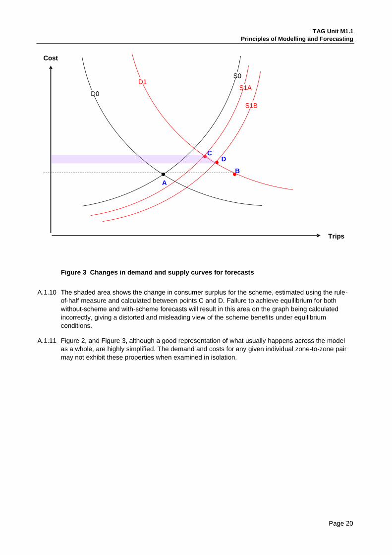
A.1.8 Figure 3 extends Figure 2 with typical demand and supply curves for future year forecasts:

• Curves D0 and S0 represent the demand and supply curves respectively for the model base

year, previously shown in Figure 2.

• Curve D1 represents the demand for a future forecast year. Typically, demand is higher than the

base year due to changes in population, employment and income;.

• Curves S1A and S1B represent the supply curves for the without-scheme and with-scheme

forecasts respectively. Typically the supply curve for the without-scheme case will be lower than

the base year, as some network improvements may be planned to accommodate increased

demand. If the scheme increases capacity and/or speed of travel, the cost will be reduced

further, leading to the with-scheme case having a supply curve still lower than the without-

scheme case.

A.1.9 The model runs are represented in the diagram as follows:

• point A is the equilibrium point in the base year;

• point B is the reference forecast, representing future year demand, under the assumption that

costs do not change from the base year. This forecast is not in equilibrium (hence it does not

intersect with any supply curves);

• point C is the without-scheme forecast, representing future year demand and supply in the

absence of the scheme; and

• point D is the with-scheme forecast, representing future year demand and supply with the

scheme in place.

Page 19

TAG Unit M1.1

Principles of Modelling and Forecasting

A

B

Trips

Cost

C D

S0

S1A D0

D1

S1B

Figure 3 Changes in demand and supply curves for forecasts

A.1.10 The shaded area shows the change in consumer surplus for the scheme, estimated using the rule-

of-half measure and calculated between points C and D. Failure to achieve equilibrium for both

without-scheme and with-scheme forecasts will result in this area on the graph being calculated

incorrectly, giving a distorted and misleading view of the scheme benefits under equilibrium

conditions.

A.1.11 Figure 2, and Figure 3, although a good representation of what usually happens across the model

as a whole, are highly simplified. The demand and costs for any given individual zone-to-zone pair

may not exhibit these properties when examined in isolation.

Page 20

TAG Unit M1.1

Principles of Modelling and Forecasting

Appendix B The Production / Attraction definition

B.1.1 The Production / Attraction (or P/A) definition is used to represent the various trips that form a tour

(whether outbound from home, return to home, or non-home-based) in such a way that relates them

most closely to the available demographic data. As the strongest and most relevant demographic

data generally relates to resident population, it is useful to distinguish trip ends that relate to “home” from those that relate to “non-home” activities.

B.1.2 The shortest, and most common, pattern for a tour has two trips – an outbound trip from home to

an activity, and a return trip from the activity to home. Both of these are home-based trips with

one end at home, and these are distinguished from non-home-based trips which have neither end

at home. Tours with three or more trips have an outbound trip to the first activity, followed by a

series of non-home-based trips to the other activities, and ending with a return trip from the final

activity to home.

B.1.3 Home-based trip ends are split by production (home) and attraction (the reason for travel). Across

a suitably large geographical area, it is usually best to scale the attractions to match the

productions, as the productions are based on the most relevant and reliable data (resident

population) and the fit of production trip ends to planning assumptions is usually better.

B.1.4 In theory there are various ways of defining the productions and attractions for non-home-based

trips, but TAG and the Department’s trip end forecasting dataset NTEM (National Trip End Model) uses the simplest possible definition, as follows:

• the production is defined to be the origin of the trip; and

• the attraction is defined to be the destination of the trip.

B.1.5 An example relating the P/A definition to the origin-destination (O/D) definition is shown in Figure 4.

P A

O D O D

Home Work

Home Work Work Home

Offpeak AM peak Interpeak PM peak Offpeak

P A

O D

Work Shop

Work Shop

HBW NHBShop NHBW HBW

P A

O D

Shop Work

Shop Work

From home to work From work to shop From shop to work From work to home

A P

Work Home

Figure 4 Example of P/As and O/Ds for a sequence of trips

Page 21