Tackling Poverty and Social Impacts: Philippine Response

to the Global Economic Crisis

Arsenio M. Balisacan with

Sharon Faye Piza Dennis Mapa

Carlos Abad Santos and

Donna Mae Odra

1 June 2010

Note: Part of this report has also drawn substantially from the authors’ ongoing work for the Asian Development Bank. The authors thank both UNDP and ADB for financial support. This report was partially funded through a contribution from the Government of Norway. It is part of a series of crisis response PSIA initiatives aimed at generating policy responses to protect human development gains and to stimulate a broader policy dialogue. The Poverty Group at UNDP manages the PSIA initiative and provides technical guidance to country teams conducting the analysis. The views and interpretations expressed in this report are those of the authors and should not be attributed to either organization.

2

1. Introduction

Much has been written about the origin, spread, and ramifications of the global economic crisis (GEC) in 2008/2009. When the crisis erupted in mid-2008, most observers in the development community contended that the global economy would slide to recession and that it would take at best a couple of years or at worst several years, as in the Great Depression of the 1930s, for the world economy to fully recover lost ground. No Asian economy, big or small, was expected to be spared from the fallout of the crisis. Yet, economic performance data in the second half of 2009 showed positive indications that the worst is over and that the major economies are on their way to recovery, thanks to generally synchronized fiscal stimulus programs aimed at reviving growth in these economies. This is more so in Asia, particularly China, India, and Indonesia where economic growth continued to be comparatively robust, albeit less spectacular than their customary levels in the past two decades. The Philippine economy has also avoided the recession, although the full impact of its sharp slowdown on various population groups, particularly the poor, remains to be ascertained. One common view is that the global crisis has hit most adversely the workers in the export sector, particularly manufactured exports, and overseas Filipino workers (OFWs), as consumer demands and incomes in the country’s major trading partners contracted. The initial waves of layoffs and labor displacements from these sectors, as well as the declines in the rate of remittance inflows, have occupied front pages of national dailies. However, it is possible that the channels by which the crisis affected various population groups have been more complex and less visible than those impressed in the public’s mind by media. Moreover, household responses to the crisis could have also varied quite enormously, even among the poor, owing to differences in household attributes, socioeconomic circumstances, and location. For many households, as the experiences from past financial and economic crises (e.g., the Asian financial crisis in 1997/1998) suggest, the consequence of the crisis may linger for a long time, even beyond a generation, such as when children are withdrawn from schools or receive inadequate food for balanced nutrition. Furthermore, the government’s response to the crisis, especially through its fiscal stimulus program, may have also influenced the incidence, depth, and severity of impact across sectors and population groups.

At least two other major developments prior to the GEC could have likewise influenced the impact of the shock on poverty. One was the sharp spikes in global foodgrain prices in late 2007 and the first half of 2008 owing to a confluence of global supply and demand factors. Although the government intervened aggressively in the domestic market to cushion the impact of the shock, particularly on the poor, domestic rice prices rose by about 40% during the period. Second, in the seven-year period prior to the food price shock, poverty was disturbingly rising even as the economy was growing at a rate (averaging 4.8% a year) faster than the country’s population growth rate (2% a year). Both these developments could have made the poor even more vulnerable to the GEC.

Clearly, understanding the impact of external shocks such as the GEC on poverty, particularly their differential effects across population groups and social divides, is crucial to the design of a development strategy aimed at fostering a more inclusive growth, thereby speeding up the pace of poverty reduction. This study goes beyond anecdotal evidence characteristic of many previous accounts on the social impact of the GEC by systematically examining the evidence and recent data and drawing policy lessons and recommendations toward improved poverty-

3

mitigating responses to financial and economic shocks. The next section of this report provides an overview of the country’s economic performance before and during the GEC. It then discusses the empirical approach used to assess the impact of the crisis on the economy and poverty. The subsequent two sections show the findings of the study based on examination of macroeconomic data and panel survey data. The discussion of crisis impact focuses on economic performance (major components of GDP and employment) and the evolution of poverty during the crisis across social divides. The report then assesses the effectiveness of the government’s response to the crisis in terms of key programs. The last section summarizes the findings and presents their implications for policy reform and design of poverty reduction programs.

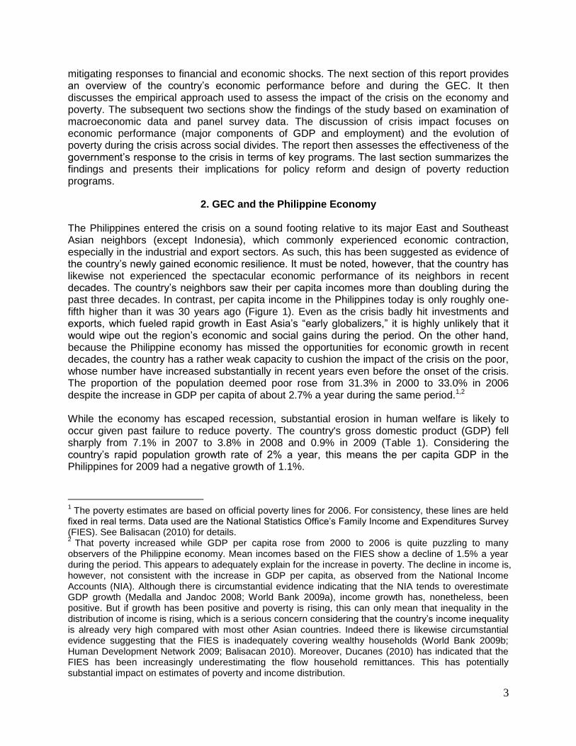
2. GEC and the Philippine Economy The Philippines entered the crisis on a sound footing relative to its major East and Southeast Asian neighbors (except Indonesia), which commonly experienced economic contraction, especially in the industrial and export sectors. As such, this has been suggested as evidence of the country’s newly gained economic resilience. It must be noted, however, that the country has likewise not experienced the spectacular economic performance of its neighbors in recent decades. The country’s neighbors saw their per capita incomes more than doubling during the past three decades. In contrast, per capita income in the Philippines today is only roughly one-fifth higher than it was 30 years ago (Figure 1). Even as the crisis badly hit investments and exports, which fueled rapid growth in East Asia’s ―early globalizers,‖ it is highly unlikely that it would wipe out the region’s economic and social gains during the period. On the other hand, because the Philippine economy has missed the opportunities for economic growth in recent decades, the country has a rather weak capacity to cushion the impact of the crisis on the poor, whose number have increased substantially in recent years even before the onset of the crisis. The proportion of the population deemed poor rose from 31.3% in 2000 to 33.0% in 2006 despite the increase in GDP per capita of about 2.7% a year during the same period.1,2 While the economy has escaped recession, substantial erosion in human welfare is likely to occur given past failure to reduce poverty. The country's gross domestic product (GDP) fell sharply from 7.1% in 2007 to 3.8% in 2008 and 0.9% in 2009 (Table 1). Considering the country’s rapid population growth rate of 2% a year, this means the per capita GDP in the Philippines for 2009 had a negative growth of 1.1%.

1 The poverty estimates are based on official poverty lines for 2006. For consistency, these lines are held

fixed in real terms. Data used are the National Statistics Office’s Family Income and Expenditures Survey (FIES). See Balisacan (2010) for details. 2 That poverty increased while GDP per capita rose from 2000 to 2006 is quite puzzling to many

observers of the Philippine economy. Mean incomes based on the FIES show a decline of 1.5% a year during the period. This appears to adequately explain for the increase in poverty. The decline in income is, however, not consistent with the increase in GDP per capita, as observed from the National Income Accounts (NIA). Although there is circumstantial evidence indicating that the NIA tends to overestimate GDP growth (Medalla and Jandoc 2008; World Bank 2009a), income growth has, nonetheless, been positive. But if growth has been positive and poverty is rising, this can only mean that inequality in the distribution of income is rising, which is a serious concern considering that the country’s income inequality is already very high compared with most other Asian countries. Indeed there is likewise circumstantial evidence suggesting that the FIES is inadequately covering wealthy households (World Bank 2009b; Human Development Network 2009; Balisacan 2010). Moreover, Ducanes (2010) has indicated that the FIES has been increasingly underestimating the flow household remittances. This has potentially substantial impact on estimates of poverty and income distribution.

4

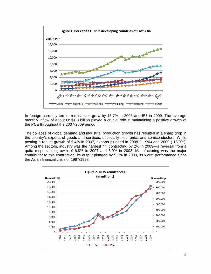
More can be learned from examining the components of GDP before and after the crisis. As expected, the deceleration of GDP is reflected in personal consumption expenditure (PCE), which contributed about three-fourths of GDP for the past 10 years. PCE growth dropped sharply from 5.8% in 2007 to 4.7% in 2008 and 3.7% in 2009, in spite of the inflow of OFW remittances. Contrary to the common view that the crisis would cause OFW remittances to fall sharply, remittances, whether measured in foreign currency (US dollars) or local currency (Philippine peso), continued to grow in 2008 and 2009, although at a much lower rate (Figure 2).

Table 1. Growth rates of GDP and its components

Year/Quarter GDP Sector Expenditure

Agri Industry Manuf Services PCE GC CF X M

1990-1999 2.8 1.5 2.5 2.3 3.7 3.7 3.5 3.2 6.6 7.2

2000 6.0 4.3 9.0 5.6 4.4 3.5 6.1 23.9 17.0 4.3

2001 1.8 3.7 -2.5 2.9 4.3 3.6 -5.3 -7.3 -3.4 3.5

2002 4.4 4.0 3.9 3.5 5.1 4.1 -3.8 -4.3 4.0 5.6

2003 4.9 3.8 4.0 4.2 6.1 5.3 2.6 3.0 4.9 10.8

2004 6.4 5.2 5.2 5.8 7.7 5.9 1.4 7.2 15.0 5.8

2005 5.0 2.0 3.8 5.3 7.0 4.8 2.3 -8.8 4.8 2.4

2006 5.3 3.8 4.5 4.6 6.5 5.5 10.4 5.1 13.4 1.8

Q1 5.5 3.4 5.3 4.6 6.5 5.2 9.5 1.5 13.1 2.8

Q2 5.3 7.4 3.9 3.0 5.5 5.2 8.1 2.3 24.9 4.2

Q3 5.2 3.7 5.2 4.4 5.6 5.3 14.6 13.7 10.5 0.8

Q4 5.4 1.7 3.8 4.7 8.2 6.2 9.8 3.9 6.0 -0.2

2007 7.1 4.8 6.8 3.4 8.1 5.8 6.6 12.4 5.4 -4.1

Q1 6.9 4.0 6.3 3.6 8.5 5.9 12.1 18.1 10.5 -1.8

Q2 8.3 3.8 10.6 3.8 8.4 5.6 8.9 17.4 4.2 -10.2

Q3 6.8 5.6 5.7 3.1 8.1 5.7 -2.6 5.3 3.3 -4.7

Q4 6.3 5.7 4.7 2.7 7.7 6.2 8.0 7.1 4.5 0.7

2008 3.8 3.2 5.0 4.3 3.3 4.7 3.2 1.7 -1.9 2.4

Q1 3.9 2.8 2.7 2.4 5.2 5.1 -0.3 -1.7 -7.7 -2.6

Q2 4.2 4.9 4.0 6.1 4.0 4.1 0.0 13.6 6.1 0.0

Q3 4.6 2.5 7.6 5.4 3.3 4.4 11.8 9.4 3.3 6.7

Q4 2.9 2.9 5.3 3.4 1.3 5.0 2.5 -11.7 -11.5 5.0

2009 0.9 0.2 -2.0 -5.2 3.2 3.7 8.6 -9.6 -13.9 -6.3

Q1 0.6 2.1 -2.5 -7.3 2.0 1.3 4.5 -15.1 -14.7 -20.6

Q2 0.8 0.2 -1.7 -7.2 2.7 5.4 9.7 -10.3 -18.1 -2.2

Q3 0.4 1.5 -5.0 -7.8 3.8 3.2 8.1 -12.1 -13.0 0.1

Q4 1.8 -2.8 1.1 1.3 4.2 5.1 12.1 -0.8 -10.0 -2.5

Note: Quarterly figures are year-on-year growth rates. Manufacturing is a component of Industry. PCE=personal consumption expenditures; GC=government consumption; CF=capital formation; X=exports; M=imports.

Source: National Statistical Coordination Board.

5

In foreign currency terms, remittances grew by 13.7% in 2008 and 5% in 2009. The average monthly inflow of about US$1.3 billion played a crucial role in maintaining a positive growth of the PCE throughout the 2007-2009 period. The collapse of global demand and industrial production growth has resulted in a sharp drop in the country’s exports of goods and services, especially electronics and semiconductors. While posting a robust growth of 5.4% in 2007, exports plunged in 2008 (-1.9%) and 2009 (-13.9%). Among the sectors, industry was the hardest hit, contracting by 2% in 2009—a reversal from a quite respectable growth of 6.8% in 2007 and 5.0% in 2008. Manufacturing was the major contributor to this contraction; its output plunged by 5.2% in 2009, its worst performance since the Asian financial crisis of 1997/1998.

0

2,000

4,000

6,000

8,000

10,000

12,000

14,000

2005 $ PPP

Figure 1. Per capita GDP in developing countries of East Asia

China Indonesia Malaysia Philippines Thailand Vietnam

0

100,000

200,000

300,000

400,000

500,000

600,000

700,000

800,000

900,000

0

2,000

4,000

6,000

8,000

10,000

12,000

14,000

16,000

18,000

20,000

19

90

19

91

19

92

19

93

19

94

19

95

19

96

19

97

19

98

19

99

20

00

20

01

20

02

20

03

20

04

20

05

20

06

20

07

20

08

20

09

Nominal PhpNominal US$

Figure 2. OFW remittances(in millions)

US$ Php

6

In previous episodes of financial and macroeconomic crises, the agriculture sector proved comparatively resilient to the shocks. Even during the Asian financial crisis of 1997/1998, the poor performance of the agriculture sector was related more to the widespread drought induced by the El Nino phenomenon than to the external shock (Balisacan and Edillon 2001; Datt and Hoogeveen 1999). The sector again did not contract as the GFC swept across the domestic economy, although its growth substantially decelerated from 4.8% in 2007 to 3.2% in 2008 and then sharply to 0.2% in 2009. The sharp drop in 2009 was due largely to the devastation in Luzon unleashed by three major typhoons in the second half of the year. Farm devastation caused agricultural output to shrink by 2.5% in the fourth quarter of 2009 (year-on-year basis).

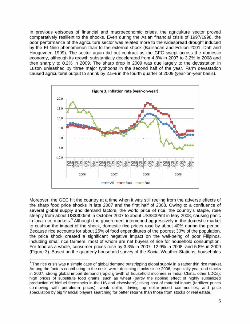
Moreover, the GEC hit the country at a time when it was still reeling from the adverse effects of the sharp food price shocks in late 2007 and the first half of 2008. Owing to a confluence of several global supply and demand factors, the world price of rice, the country’s staple, rose steeply from about US$300/mt in October 2007 to about US$800/mt in May 2008, causing panic in local rice markets.3 Although the government intervened aggressively in the domestic market to cushion the impact of the shock, domestic rice prices rose by about 40% during the period. Because rice accounts for about 25% of food expenditures of the poorest 30% of the population, the price shock created a significant negative impact on the well-being of poor Filipinos, including small rice farmers, most of whom are net buyers of rice for household consumption. For food as a whole, consumer prices rose by 3.3% in 2007, 12.9% in 2008, and 5.8% in 2009 (Figure 3). Based on the quarterly household survey of the Social Weather Stations, households

3 The rice crisis was a simple case of global demand outstripping global supply in a rather thin rice market.

Among the factors contributing to the crisis were: declining stocks since 2006, especially year-end stocks in 2007; strong global import demand (rapid growth of household incomes in India, China, other LDCs); high prices of substitute food grains, such as wheat (partly the rippling effect of highly subsidized production of biofuel feedstocks in the US and elsewhere); rising cost of material inputs (fertilizer prices co-moving with petroleum prices); weak dollar, driving up dollar-priced commodities; and price speculation by big financial players searching for better returns than those from stocks or real estate.

-10.0

-5.0

0.0

5.0

10.0

15.0

20.0

JAN

FEB

MA

RA

PR

MA

YJU

NJU

LA

UG

SEP

OC

TN

OV

DEC

JAN

FEB

MA

RA

PR

MA

YJU

NJU

LA

UG

SEP

OC

TN

OV

DEC

JAN

FEB

MA

RA

PR

MA

YJU

NJU

LA

UG

SEP

OC

TN

OV

DEC

JAN

FEB

MA

RA

PR

MA

YJU

NJU

LA

UG

SEP

OC

TN

OV

DEC

2006 2007 2008 2009

Figure 3. Inflation rate (year-on-year)

All Food Fuel

7

experiencing hunger (expressed as a proportion of total households) rose during this period, reaching an unprecedented high of 23.7% in the last quarter of 2008 since SWS started monitoring the series in July 1998.4 Surprisingly, beyond the aggregate data, not much is known about the differential effects of this shock on various population groups and on the food economy, including any ramifications caused by sharply rising fuel prices in the global market. Nor has there been a systematic assessment on the efficacy and income distribution effects of the government’s response to the food crisis.

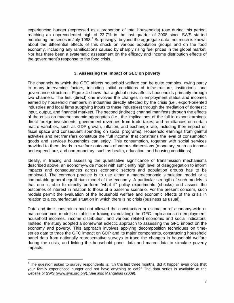
3. Assessing the impact of GEC on poverty The channels by which the GEC affects household welfare can be quite complex, owing partly to many intervening factors, including initial conditions of infrastructure, institutions, and governance structures. Figure 4 shows that a global crisis affects households primarily through two channels. The first (direct) one involves the changes in employment status and incomes earned by household members in industries directly affected by the crisis (i.e., export-oriented industries and local firms supplying inputs to these industries) through the mediation of domestic input, output, and financial markets. The second (indirect) channel manifests through the effects of the crisis on macroeconomic aggregates (i.e., the implications of the fall in export earnings, direct foreign investments, government revenues from trade taxes, and remittances on certain macro variables, such as GDP growth, inflation, and exchange rate, including their impact on fiscal space and consequent spending on social programs). Household earnings from gainful activities and net transfers constitute the ―full income‖ that constrains the level of consumption goods and services households can enjoy. This consumption, together with social services provided to them, leads to welfare outcomes of various dimensions (monetary, such as income and expenditure, and non-monetary, such as health, education, and housing conditions). Ideally, in tracing and assessing the quantitative significance of transmission mechanisms described above, an economy-wide model with sufficiently high level of disaggregation to inform impacts and consequences across economic sectors and population groups has to be employed. The common practice is to use either a macroeconomic simulation model or a computable general equilibrium model of the economy. A particular strength of such models is that one is able to directly perform ―what if‖ policy experiments (shocks) and assess the outcomes of interest in relation to those of a baseline scenario. For the present concern, such models permit the evaluation of the household welfare and economic effects of the crisis in relation to a counterfactual situation in which there is no crisis (business as usual). Data and time constraints had not allowed the construction or estimation of economy-wide or macroeconomic models suitable for tracing (simulating) the GFC implications on employment, household incomes, income distribution, and various related economic and social indicators. Instead, the study adopted a somewhat eclectic approach to assessing the GFC impact on the economy and poverty. This approach involves applying decomposition techniques on time-series data to trace the GFC impact on GDP and its major components, constructing household panel data from nationally representative surveys to trace the changes in household welfare during the crisis, and linking the household panel data and macro data to simulate poverty impacts.

4 The question asked to survey respondents is: “In the last three months, did it happen even once that

your family experienced hunger and not have anything to eat?” The data series is available at the website of SWS (www.sws.org.ph/). See also Mangahas (2009).

8

Figure 4. Channels by which the global financial crisis affects household welfare.

Global Financial

& Economic

Crisis

Domestic markets

Outputs Inputs Labor (migration) Finance/credit

Government response (fiscal /monetary

stimulus)

Social services

Public health Education Housing Water & sanitation

Welfare Outcomes

Non-monetary Literacy Health & nutrition Empowerment

Monetary Income Expenditure

Household decisions

Earned income

Net transfer (private + public)

Full income

Macro impact

Foreign investments

Export earnings Import taxes Remittances ----------------------- GDP growth Inflation Exchange rates

9

4. Impact on the economy It is tempting to attribute the observed sharp slowdown of GDP and its components to the GEC. Surprisingly, this attribution is not uncommon, even among serious observers of the Philippine economy. This is, however, wrong. One should instead ask: if the GEC did not occur, what would have been the performance of the Philippine economy? Would the GDP growth of 7.1% achieved in 2007 have continued in the succeeding years? In other words, was the growth sustainable? If not sustainable (i.e., the comparatively high growth rate was an aberration), the economy would be expected to slide back to its long-term growth path, with or without the shock. Indeed, many studies point out the critical structural and policy constraints preventing the economy from moving to a high-growth path as that tracked by the country’s neighbors (Magnoli 2008; World Bank 2010; Canlas et al. 2009; Balisacan and Hill 2003, 2007). For one, national savings and investment rates are extremely low by the standards of the major East Asian countries. This has resulted in low infrastructure development, particularly transport and power, and poor provision of key social services, especially basic health and education. The country’s governance structures have also created an environment of policy instability and engendered corruption and all forms of rent-seeking activities across branches and layers of the government. The challenge is to identify the potential (long-term) growth path of the economy based on information about its past performance. To do this, the study employed a decomposition technique that permits the identification of long-term (LT) trend, seasonally-adjusted (SA) trend, and random effects from the observed variable of interest. For the economic aggregates of interest to this report, the LT trend can be roughly interpreted to reflect the economy’s potential, given its resources, technologies, institutions, and policies. The SA trend, on the other hand, nets out any effects that seasonality of production and consumption may have on the same aggregate data.5 For any given quarter of the year, the difference between the LT trend and the SA trend captures the impact of the GEC and the government’s policy responses (say, fiscal stimulus package) on the shock. Given that there is a time lag between the shock and the impact of government’s interventions aimed at containing the adverse effects of the crisis, the LT-SA gap during the early quarters of the crisis years (say, the last two quarters of 2008 and first quarter of 2009) may reflect the full impact of the crisis on the variables of interest. Otherwise, if the effects of the interventions are immediate, the gap would underestimate the impact of the crisis. In the decomposition analysis that follows, the study attempts to further ―chip away‖ any effects that the government’s fiscal programs may have on the gap. Figures 5-8 show the LT and ST trends of GDP and its components, from both demand and supply sides, based on quarterly data for the period 1991-2009. In these figures, the solid line represents the seasonally adjusted series while the dotted line represents the long term trend. Comparing the values of the seasonally-adjusted GDP and its long-term trend for the crisis period, one can see that the seasonally-adjusted GDP fell below its long-term trend beginning in the fourth quarter of 2008 up to the fourth quarter of 2009. The seasonally-adjusted GDP is lower than its long run trend by about 0.3% in the fourth quarter of 2008, 2.9% in first quarter of 2009, 2.3% in the second quarter, 3.0% in the third quarter, and 3.1% in the fourth quarter. Put differently, the crisis pushed down the GDP growth rate from its long-term trend (estimated to be about 4.7%) by 1.0 percentage point in 2008 and 3.8 percentage points in 2009.

5 The seasonally adjusted series were generated using the U.S. Census Bureau’s X12 seasonal

adjustment program from within EViews Version 6.0 (Quantitative Micro Software). The long term trend component of the time series is extracted using the Hodrick-Prescott (HP) filter. See Annex A for details of the estimation and data.

10

As expected, industry was the hardest hit by the crisis. SA output declined relative to its long-term trend in the four quarter of 2009: by 5.3% in the first quarter, 2.7% in the second quarter, 5.0% in the third quarter, and 1.8% in the fourth quarter. In terms of growth forgone, the industry’s growth rate in 2009 was 6.0 percentage points lower than the sector’s long-term growth potential. The decline in its manufacturing sub-sector was particularly sharp, hitting 7.7 percentage points.

40,000

60,000

80,000

100,000

120,000

140,000

160,000

180,000

200,000

Q1

Q2

Q3

Q4

Q1

Q2

Q3

Q4

Q1

Q2

Q3

Q4

Q1

Q2

Q3

Q4

Q1

Q2

Q3

Q4

Q1

Q2

Q3

Q4

Q1

Q2

Q3

Q4

Q1

Q2

Q3

Q4

Q1

Q2

Q3

Q4

Q1

Q2

Q3

Q4

2000 2001 2002 2003 2004 2005 2006 2007 2008 2009

In 1

98

5 m

illio

n p

eso

s

Figure 6. Long-term and seasonally adjusted GDP by sector

Agriculture Industry Manufacturing Services

200,000

240,000

280,000

320,000

360,000

400,000

Q1

Q2

Q3

Q4

Q1

Q2

Q3

Q4

Q1

Q2

Q3

Q4

Q1

Q2

Q3

Q4

Q1

Q2

Q3

Q4

Q1

Q2

Q3

Q4

Q1

Q2

Q3

Q4

Q1

Q2

Q3

Q4

Q1

Q2

Q3

Q4

Q1

Q2

Q3

Q4

2000 2001 2002 2003 2004 2005 2006 2007 2008 2009

In 1

98

5 m

illio

n p

eso

s

Figure 5. Long-term and seasonally adjusted GDP, 2000-2009

Seasonally adjusted Long term trend

11

For agriculture, SA output fell below LT output starting from first quarter of 2009 up to the fourth quarter of the same, that is, by 1.0% in the first quarter, 1.4% in the second quarter, 2% in the third quarter, and, 5.2% in the fourth quarter. The last quarter’s big drop in the seasonally-adjusted AFF was largely due to the effects of the typhoons Ondoy and Pepeng. The impact on industry started in the third quarter of 2008 when the sector’s SA output declined 0.5% relative to its long-term trend. The subsequent quarterly declines were 1.5% in the fourth quarter of 2008, 2.2% in the first quarter of 2009, 2.3% in the second quarter, 2.3% in the third quarter, and 2.9% in the fourth quarter. In terms of growth forgone, the impact was a growth reduction of 2.5 percentage points in 2008 and 2.4 percentage points in 2009.

On the demand side of the national income accounts, personal consumption expenditures (PCE), the largest contributor to GDP growth, declined only modestly, relative to its long-term trend, although over a longer span of quarters. PCE fell below its long-term trend by 0.5% in the second quarter of 2008, 0.2% in the third quarter, and another 0.2% in the fourth quarter. In 2009, PCE declined by 3.8% in the first quarter, 0.6% % in the second quarter, 2.4% in the third quarter, and 0.9% in the fourth quarter, relative to the long-term trend. Expressed in terms of growth divergence, PCE growth dropped by 0.8 percentage point in 2008 and 1.7 percentage points in 2009 relative to its long-term growth trend. The drop was remarkably muted because remittances of OFWs did not slow down as sharply as expected at the onset of the crisis, as shown in section 2 above.

As shown in section 2, the government’s push to stimulate the economy through pump-priming activities is reflected in the sharp increase in government expenditures as a proportion of GDP in 2009 (Figure 8). These activities pushed up the seasonally-adjusted GCE, relative to its long-term trend, in the last three quarters of 2009. The seasonally-adjusted GCE is higher than its long-term trend by 2.4% in the second quarter, 3.3% in the third quarter, and 5.5% in the fourth quarter. The relatively high figure in the fourth quarter is mainly due to the disbursement of

0

50,000

100,000

150,000

200,000

250,000

300,000

350,000

Q1

Q2

Q3

Q4

Q1

Q2

Q3

Q4

Q1

Q2

Q3

Q4

Q1

Q2

Q3

Q4

Q1

Q2

Q3

Q4

Q1

Q2

Q3

Q4

Q1

Q2

Q3

Q4

Q1

Q2

Q3

Q4

Q1

Q2

Q3

Q4

Q1

Q2

Q3

Q4

2000 2001 2002 2003 2004 2005 2006 2007 2008 2009

In 1

98

5 m

illio

n p

eso

s

Figure 7. Long-term and seasonally adjusted GDP by expenditure type

PCE Government Capital formation Exports Imports

12

funds for relief and rehabilitation of areas affected by tropical storms Ondoy and Pepeng. Overall, while the growth of government expenditures in 2008 was less than its long-term trend; that in 2009 was significantly higher by 2.8 percentage points. Moreover, fixed capital formation (FCF) and exports took the brunt of the crisis. Figure 7 shows that the seasonally-adjusted FCF declined, relative to its long-term trend, starting in the fourth quarter of 2008. The seasonally-adjusted FCF fell below its long-term trend by 6.1% in the fourth quarter of 2008. In the first quarter of 2009, the seasonally-adjusted FCF fell by a double-digit figure, at 10.7%, relative to its long-term trend. It went up by 3.5% during the second quarter before dropping again by 4.8% in the fourth quarter. The decline continued in the fourth quarter, by 6.7%. Expressed in growth terms, PCF grew close to its long-term pace in 2008 but dropped by 9.9% in 2009. For exports, the decline relative to the long-term trend was 3.8% in the fourth quarter of 2008. In 2009, SA exports declined by 12.1% in the first quarter, 9.0% in the second quarter, 7.5% in the third quarter, and 12.9% in the fourth quarter.

The movement of labor during the GEC can be gleaned from the Labor Force Surveys conducted quarterly by NSO. These surveys show no drastic changes in the employment figures, at least in so far as national averages are concerned (Table 2). Despite the noticeable growth in the labor force, unemployment rates did not increase relative to average rates in preceding years. Note, however, that underemployment rates were on the high side at the height of the crisis in 2009. ILO (2009) reported that the number of part-time workers (i.e., worked for less than 40 hours per week) shot up by more than two million between January and April 2009. Employment in manufacturing suffered the most, especially in electronics and garment sectors. Note, further, that the share of new entrants among those employed has been decreasing, from 2.4% before the GEC to 1.5% in 2008 and further down to 1.3% in 2009.

15,000

17,000

19,000

21,000

23,000

25,000

27,000

29,000

Q1

Q2

Q3

Q4

Q1

Q2

Q3

Q4

Q1

Q2

Q3

Q4

Q1

Q2

Q3

Q4

Q1

Q2

Q3

Q4

Q1

Q2

Q3

Q4

Q1

Q2

Q3

Q4

Q1

Q2

Q3

Q4

Q1

Q2

Q3

Q4

Q1

Q2

Q3

Q4

2000 2001 2002 2003 2004 2005 2006 2007 2008 2009

In 1

98

5 m

illio

n p

eso

s

Figure 8. Long-term and seasonally adjusted government expenditures

13

Table 1. Employment shares by sector and status (in %)

Employment grouping Average

2001-2003 Average

2004-2007 2008 2009

By sector of employment

Agriculture 37.3 36.7 35.7 34.0

Industry 15.6 15.1 14.7 14.5

Manufacturing 9.6 9.3 8.4 8.3

Services 47.1 48.2 49.6 51.5

By status of employment

Formal

Employer 5.2 4.5 4.1 4.0

Wage and salary worker 44.0 45.8 46.7 47.8

Informal

Self-employed 32.6 32.1 31.4 30.5

Wage and salary worker 5.4 5.1 5.3 5.8

Unpaid 12.8 12.5 12.5 11.9

Labor force growth (in %) 3.1 1.3 3.2 3.1

Employment growth (in %) 2.8 1.6 2.6 2.7

New entrants (% of employed) 2.5 2.4 1.5 1.3

Unemployment rate 10.0 8.0 6.8 7.1

Underemployment rate 15.9 19.4 17.5 19.4

Total employment (in '000)

34,533 35,477

Source: Labor Force Surveys (October rounds), National Statistics Office

Trends in employment shares mirror the observation at the macro level discussed in the previous section. Industry’s employment share declined only slightly during the crisis, though the decline was quite substantial (about 1 percentage point drop in 2008) for its manufacturing sub-sector. Agriculture’s share continued its downward trend even during the crisis. In contrast, the employment share of industry rose during the crisis, absorbing what was shed off by the other two sectors. In 2009, industry accounted for 52% of those employed, a substantial rise from about 48% on average in 2004-2007. Contrary to common claims, formal sector employment has been rising, not falling, even during the crisis. 6 The share of formal sector employment rose from about 50% on average in 2004-2007 to 51% in 2008 and to 52% in 2009. The bulk of the change came from wage and salary workers who represented about 46% of the employed in 2004-2007, 47% in 2008, and 48% in 2009. In contrast, the combined share of the self-employed and the unpaid family workers, who accounted for the bulk of the informal sector employment, declined from about 45% on average in 2004-2007 to 44% in 2008 and to 42% in 2009. The share of the informal wage workers

6

Included here are employees from private establishments, government and government owned companies and corporations.

14

increased slightly during the crisis, but this sub-sector accounted for not more than 6% of total employment. 7 In summary, while the country avoided recession, the impact of the GEC on the economy was nonetheless severe. The crisis pushed down GDP growth rate from its long-term potential (4.7% a year) by 1.0 percentage point in 2008 and 3.8 percentage points in 2009. From the supply side, the industry, particularly manufacturing, was hit hardest, effectively reducing the sector’s output growth in 2009 by 6.0 percentage points relative to its long-term growth potential. From the demand side, the drop in PCE growth relative to long-term trend—by 0.8 percentage point in 2008 and 1.7 percentage points in 2009—was remarkably muted because remittances of OFWs did not slow down as sharply as expected at the onset of the crisis. Private capital formation and exports, however, took the brunt of the crisis. PCF grew close to its long-term pace in 2008 but dropped by 9.9% in 2009. Exports shrank by 1.9% in 2008 and 14.2% in 2009. While the growth of government expenditures in 2008 was less than its long-term trend, that in 2009 was significantly higher by 2.8 percentage points. In the next section, these results are used to inform the impact of the crisis on poverty across population groups and social divides. Employment indicators showed no drastic changes during the crisis. Employment share in industry dropped noticeably starting in 2008, which mirrored the drop of output in the sector. Unemployment rate increased in 2009 from its level in the previous year but still at a lower rate than those posted before the crisis. There was no noticeable shift of employment from the formal to the informal sector as often commonly claimed in accounts of the crisis. Underemployment, however, were on the high side at the height of the crisis.

5. Impact on poverty across social divides Little is known about the changes in the level and incidence of poverty in the Philippines during the GEC. Even less is known about the dynamics of poverty across population groups and social divides. Such understanding has been largely constrained by the absence of nationally representative, comparable household surveys on incomes and expenditures covering the pre-crisis and crisis periods. The latest data available for poverty comparison are from the 2006 Family Income and Expenditures Survey (FIES) of the National Statistics Office.8 While the 2009 FIES has been conducted, the public-use file that will prove useful for poverty comparison is not yet available. Ideally, in understanding the dynamics of poverty during a crisis, one has to have a household panel data, i.e., the same households interviewed repeatedly over time. Such data set will be even more useful in informing policy choices if it is also nationally representative. The effort to construct such a household panel data set and use it to examine the impact of the crisis across social divides is described below. As the effort yielded only panel data covering 2006, 2007, and 2008, results in section 4 were used to ―augment‖ the data to ―approximate‖ household welfare levels for 2009.

7 Employees of family owned businesses including employees of private households.

8 To be sure, the Social Weather Stations has a quarterly series on self-rated poverty covering the crisis

period. However, because the sample size is relatively small, the data cannot be disaggregated into finer groupings suitable for understanding poverty dynamics across social divides.

15

5.1 Constructing the “augmented” panel data The household surveys conducted by the National Statistics Office (NSO) use a master sample to draw respondents for the respective surveys. Since the NSO started implementing this sampling approach in 2003, about 20% of the total sample is kept in each survey for a period of time,9 which allows panel analysis for a considerable number of households. Among these household surveys, two collect information on household welfare: the FIES and the Annual Poverty Indicators Survey (APIS). The FIES is conducted every three years and the APIS, every year in between FIES surveys. Another survey, the Labor Force Survey (LFS), coincidental to the FIES or APIS,10 is also part of the panel. The LFS provides information on employment status of each household member. Data from the following surveys were obtained to form the panel data for the analysis:

2006 Family and Expenditure Expenditures Survey

2007 January, July and 2008 July Labor Force Surveys

2007 and 2008 Annual Poverty Indicators Surveys

About 12,000 households were marked by NSO as part of the panel in 2006. Over three years after accounting for attrition, only 8,010 households composed the panel.11 Information from these surveys provides the status of households prior to the crisis. For the purposes of this report, household income adjusted for family size is used as a proxy measure of individual welfare. This poses a problem, however, on the comparability of the FIES and APIS panel data, primarily because the administration of these two surveys differs in two aspects. First, FIES is collected in two rounds. The first round, conducted in July, covers the first semester (January to June) while the second round, conducted in January of the following year, covers the second semester (July to December). On the other hand, APIS is collected only once, every July, with the first semester as its reference period. Data collected in FIES for both rounds are tallied to come up with the annual estimates in contrast to the APIS’ first semester estimates multiplied twice for the annual estimates.12 Second, the questionnaire module for both income and expenditure in FIES is more extensive than the modules in APIS. To cite an example, in the APIS, survey respondents are asked about major aggregates only of entrepreneurial incomes, while in the FIES, they are asked a detailed listing of gross revenues and expenses for

9 The duration depends on the sample rotation. The same household can be included in various surveys

up to three years. 10

The APIS is conducted every July, coinciding with the July round of the Labor Force Survey. The FIES is fielded twice and coincides with the LFS July round of the current year and January round of the following year, although NSO uses the January round in merged datasets. 11

Household incomes from the panel sample are significantly the same with the incomes from the full sample (Wilcoxon two-sample test two-sided Pr > |Z| 0.5826). Furthermore, the Kruskal-Wallis test (Pr > Chi-Square 0.5826) shows that the distribution of the two samples are the same. 12

Fuwa (2007) examined the direction of possible bias if only one survey round is used to estimate annual income (expenditure). Using the 2003 FIES, he found that the ratio of the second to the first visit household income in the NCR region was 0.939 (consumption) or 0.987 (income) on average. One pattern that appears to be systematic (observed both in expenditure and income) is that the ratio of the second to the first visit is lower among poorer (income or expenditure) quintiles and becomes increasingly higher among higher quintiles. For example, based on the 2003 NCR sample, the ratio of the second to the first visit consumption is 0.794 among the lowest quintile while the ratio is 0.983 among the highest quintile.

16

entrepreneurial activities. Evidently, comparing income or expenditure estimates from these two sources is inappropriate13. On the other hand, APIS is collected only once, every July, with the first semester as its reference period. Data collected in FIES for both rounds are tallied to come up with the annual estimates in contrast to the APIS’ first semester estimates multiplied twice for the annual estimates.14 Second, the questionnaire module for both income and expenditure in FIES is more extensive than the modules in APIS. To cite an example, in the APIS, survey respondents are asked about major aggregates only of entrepreneurial incomes, while in the FIES, they are asked a detailed listing of gross revenues and expenses for entrepreneurial activities. Evidently, comparing income or expenditure estimates from these two sources is inappropriate.15 To make the income data in APIS comparable with those in FIES, the reported income data in the FIES panel were scaled downward by the extent of the ―measurement bias‖ but done in such a way that the income distribution observed in the panel data is preserved. The process involves (i) estimating a Mincerian earnings function using the 2006 FIES panel data on the assumption that the income variables from these data are correctly measured, (ii) applying the estimated parameters of this function to the 2007 APIS panel data to generate predicted incomes that are quite comparable to FIES incomes for 2006, and (iii) scaling down the observed FIES income data to the extent consistent with growth estimates based on predicted incomes for 2006 and 2007.16 As noted above, the household panel data set does not cover 2009. In ―augmenting‖ the panel to include this year, the study projected household incomes from the 2008 APIS using the growth estimates of GDP components derived in section 2 of this report. That is, household incomes from various sources were assumed to grow at the same rates observed for the various production-side components of the national income accounts.17 The nominal incomes in the panel data were adjusted for their real values (purchasing power) using household-specific consumer price indices. The variation in the price indices reflect varying consumption patterns across households of different income levels, family composition and characteristics, location, and preferences. In this study, the adjusted or real incomes represent a broad measure of household welfare.

13

Average per capita income based in 2007 APIS suggests a 9% drop from the average per capita income level based on FIES 2006. 14

Fuwa (2007) examined the direction of possible bias if only one survey round is used to estimate annual income (expenditure). Using the 2003 FIES, he found that the ratio of the second to the first visit household income in the NCR region was 0.987 on average. For household expenditure, the corresponding ratio was 0.939 on average. One pattern that appears to be systematic (observed both in expenditure and income) is that the ratio of the second to the first visit is lower among poorer (income or expenditure) quintiles and becomes increasingly higher among higher quintiles. For example, based on the 2003 NCR sample, the ratio of the second to the first visit consumption is 0.794 among the lowest quintile while the ratio is 0.983 among the highest quintile. 15

Average per capita income based in 2007 APIS suggests a 9% drop from the average per capita income level based on FIES 2006. In contrast, the average per capita GDP increased, in real terms, by 5% and that of average per capita PCE (personal consumption expenditure of the national income accounts) by 3.7% during this period (see Table 1). 16

See Annex B of Balisacan et al. (2010) for details of the estimation procedure. 17

Annex C of Balisacan et al. (2010) provides the details of the panel augmentation.

17

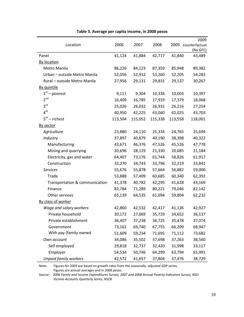
For comparability of the poverty estimates based on the panel data with the ―official‖ estimates based on the full FIES, the panel income data are calibrated in such a way that the poverty-incidence estimate from the panel data for 2006 is approximately equal to that from the full 2006 FIES data. All poverty estimates are based on official poverty lines for 2006. For consistency, these lines are held fixed in real terms. By construction, the resulting poverty estimates are not strictly comparable with officially published poverty estimates which are based on time-varying poverty lines (i.e., the welfare standard for poverty comparison varies from one survey year to another).18 5.2 Household income levels Prior to the crisis, average per capita income was Php42,717 (Table 3). Modest growth (about 2%) occurred beginning 2007 and extended to the following year. Rural areas registered higher growth than the other areas, with 4.2% growth in 2007 and 2.4% in 2008. Growth in urban areas outside NCR has not been as robust, with barely 1% in 2008. Among income classes, the poor (1st and 2nd quintile) experienced higher growth than those in the upper classes (11% for the 1st quintile and 7% for the 2nd quintile in 2008). Note however that incomes declined for the poorest quintile in 2007. The bulk of growth occurred in the 3rd and 4th quintiles where most of the OFWs belong. In contrast, per capita incomes in the richest quintile stagnated in 2008. Households in agriculture and services experienced positive growth. However, those in the industry sector already experienced decline in their incomes even before the crisis. Similarly, wage and salary workers and unpaid family workers experienced decline in 2008 in contrast to the own account workers’ high income growth of 6.2%. Estimated mean income declined by 2.1% in 2009. However, the levels across groups are still higher than 2007 figures. Certain exceptions can be named though, for instance, households in urban areas outside Metro Manila, which belong to the richest quintile. As expected, those that belong to the industry sector took a hit. Their income levels are lower in 2009 than in 2007 by about Php 2,500. The same is observed among wage and salary workers and substantially among unpaid family workers (about Php 4,200). 5.3 Impact on household welfare and poverty To gauge the probable impact of the GEC on poverty, a simulation of welfare levels involving a counterfactual scenario in which the crisis did not occur was performed. In this scenario, it is assumed that growth rates of the components of National Income Accounts reported in section 2 follow their long-term trend. If the crisis had not occurred, average per capita income in 2009 would have been Php 43,489, about Php1,650 more than the actual estimated income. This means a forgone income growth of almost 4%, which can be attributed as an aggregate impact of the crisis. The figure is slightly higher in urban centers than in rural areas. Coming from a high base, Metro Manila residents lost about Php 3,400, three times higher than what rural residents lost. Among income quintiles, the poorest quintile lost about 3.8% of its average income while the richer quintiles lost 4%. Since the richer households are typically urban dwellers, they lost more than the households in the poorest quintiles. Those deriving incomes from the industry sector took the biggest hit, with about 4.8% missed growth. Incomes of workers belonging to agriculture and services could have grown more by

18

See Balisacan (2010) for an assessment of approaches to poverty comparison in the Philippine context.

18

Table 3. Average per capita income, in 2008 pesos

Location 2006 2007 2008 2009 2009

counterfactual (No GFC)

Panel 41,124 41,884 42,717 41,840 43,489

By location

Metro Manila 86,226 84,123 87,359 85,948 89,382

Urban – outside Metro Manila 52,056 52,912 53,260 52,205 54,283

Rural – outside Metro Manila 27,956 29,131 29,831 29,137 30,267

By quintile

1st – poorest 9,111 9,304 10,336 10,003 10,397

2nd 16,409 16,785 17,919 17,379 18,068

3rd 25,026 26,032 26,931 26,216 27,254

4th 40,950 42,225 43,040 42,025 43,703

5th – richest 113,504 115,052 115,338 113,558 118,001

By sector

Agriculture 23,880 24,110 25,334 24,765 25,694

Industry 37,897 40,879 40,190 38,398 40,322

Manufacturing 43,671 46,376 47,526 45,526 47,778

Mining and quarrying 20,696 28,129 21,330 20,085 21,184

Electricity, gas and water 64,407 73,176 61,744 58,826 61,917

Construction 32,270 34,743 33,796 32,219 33,841

Services 55,676 55,878 57,664 56,882 59,000

Trade 53,888 57,409 60,685 60,340 62,392

Transportation & communication 41,378 40,782 42,295 41,628 43,169

Finance 82,784 71,289 80,221 79,046 82,142

Other services 65,139 64,535 61,094 59,804 62,232

By class of worker

Wage and salary workers 42,860 42,532 42,417 41,126 42,927

Private household 30,172 27,069 35,729 34,652 36,137

Private establishment 36,407 37,238 36,725 35,478 37,074

Government 73,161 69,740 67,755 66,209 68,947 With pay (family owned

business) 51,609 59,234 71,695 71,112 73,682

Own account 34,086 35,502 37,698 37,263 38,560

Self employed 29,818 32,737 32,420 31,998 33,117

Employer 54,534 50,746 64,299 63,794 65,991

Unpaid family workers 42,572 41,657 37,804 37,476 38,729

Note: Figures for 2009 are based on growth rates from the seasonally- adjusted GDP series. Figures are annual averages and in 2008 pesos. Source: 2006 Family and Income Expenditures Survey, 2007 and 2008 Annual Poverty Indicators Survey, NSO Income Accounts Quarterly Series, NSCB

19

3.7%. Taking the biggest share of the working class, incomes of wage and salary workers could have been 4.2% higher than the estimated income in 2009. Incomes of own account workers had a lesser decline by about 1% compared to wage and salary workers. Incidence of poverty had significantly dropped from its level of 33% in 2006.19 A 1.3 percentage point drop was observed in 2007 and a further 3.7 percentage point drop in 2008. Estimated incidence in 2009 is 1.6 percentage points higher than in 2008, and if the crisis did not occur, the incidence could have been down to 27.7%.

Table 4. Poverty and income distribution

Measure 2006 2007 2008 2009 2009

counterfactual (No GFC)

Poverty

Incidence 33.0 31.8 28.1 29.7 27.7

Magnitude 28,733,827 28,176,909 25,412,494 27,360,524 25,575,635

Inequality

Gini 0.494 0.494 0.481 0.485 0.484

Share of poorest quintile , % 4.7 4.4 4.8 4.8 4.8

Share of richest quintile, % 55.2 54.9 54.0 54.3 54.3

It appears that the substantial decline in poverty is also attributable to the improvement of income distribution between 2007 and 2008 as measured by the income Gini index. However, as noted in section 1 above, there are circumstantial evidence suggesting that the FIES – and, by implication, APIS, since both FIES and APIS share the same sampling frame – is inadequately covering wealthy households (World Bank 2009; Human Development Network 2009; Balisacan 2010). Moreover, Ducanes (2010) indicates that the FIES has been increasingly underestimating the flow of household remittances, especially among the high income groups. This has a potentially substantial impact on estimates of income inequality. Note, however, that if the wealthy households (or the incomes of wealthy households) have been underrepresented in the household surveys used in this study, such has little bearing on the poverty estimates since the estimation used the actual unit record data (individual households). As indicated in Table 3, what caused the poverty decline between 2007 and 2008 was the much higher growth rates of per capita income of the bottom (poorest) two quintiles of the population (about 9%) than those of the top three quintiles (about 2%). Further, in agriculture, where about two-thirds of the poor are located, per capita real incomes rose by 5%, in contrast to a decline of 1.7% in industry and a slightly lower increase of 3.2% in services.

The decline of poverty in the rural areas is remarkable. It was decreasing at an annual rate of about 3.7 percentage points between 2006 and 2008. The crisis raised the level 2 percentage

19

As noted earlier in this section, the panel income data are calibrated in such a way that the estimate of poverty incidence for 2006 from the panel data is approximately equal to that from the full FIES. This is simply to ease comparability of the panel series with what is widely known about the level of poverty in 2006.

20

points higher than the previous year. As seen in Figure 9, the decline in urban areas was at a much slower pace of 1% on the average annually. Note though that Metro Manila posted a percentage point increase in poverty in 2007.

Among the sectors, agriculture posted the biggest decline from 2006 to 2008 (about 7.5 percentage points), followed by industry (4.4 percentage points) (Figure 10). However, these two sectors took the brunt during the crisis, with at least 2.1 percentage point increase in poverty compared with only 0.9 percentage point.

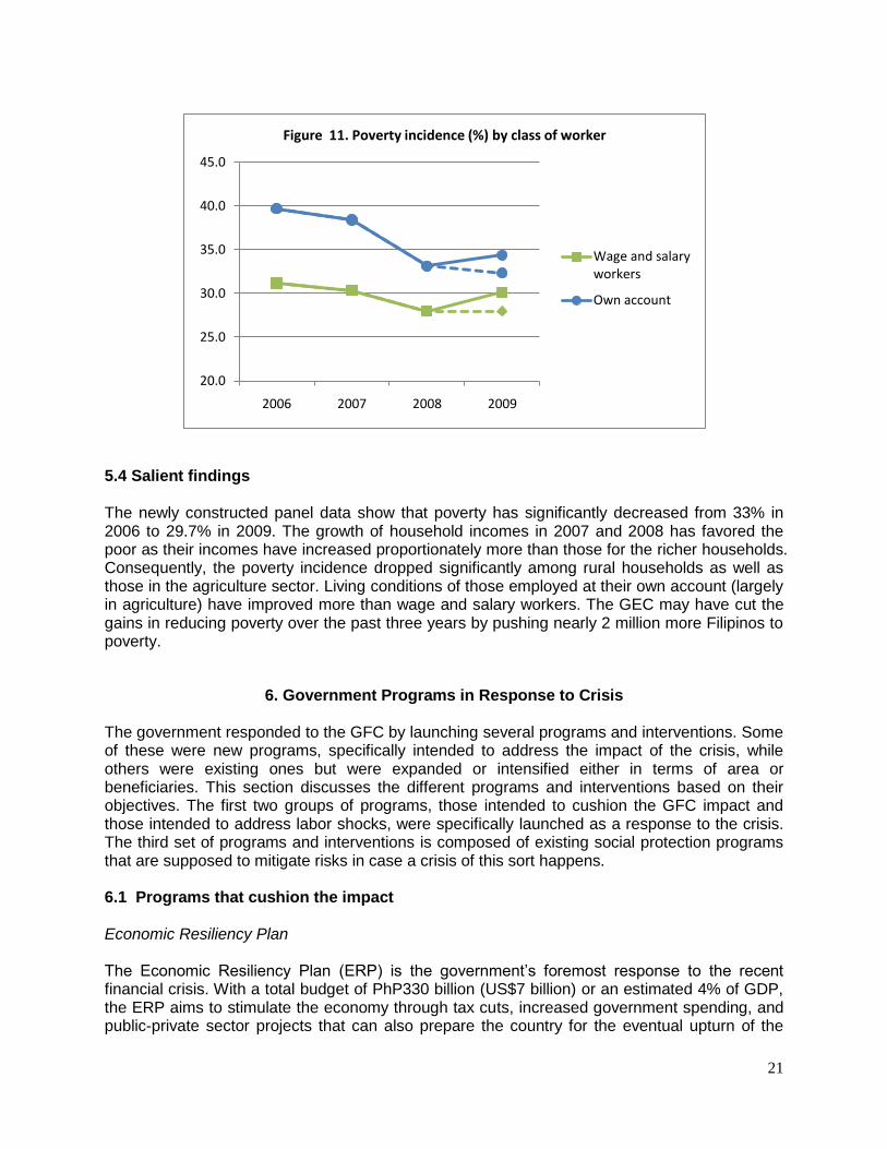
Poverty among own account workers declined substantially in 2008 (5.3 percentage points) from its level in 2007 (Figure 11). Among wage and salary workers, a modest decrease of 1.6 percentage points annually since 2006 was similarly observed. The same class of worker experienced the biggest increase (2.1 percentage points) during the crisis.

0.0

5.0

10.0

15.0

20.0

25.0

30.0

35.0

40.0

45.0

50.0

2006 2007 2008 2009

Figure 9. Poverty incidence (%) by location

Metro Manila

Urban, outside MMRural, outside MM

0.0

10.0

20.0

30.0

40.0

50.0

60.0

2006 2007 2008 2009

Figure 10. Poverty incidence by sector

Agriculture

Industry

Services

21

5.4 Salient findings The newly constructed panel data show that poverty has significantly decreased from 33% in 2006 to 29.7% in 2009. The growth of household incomes in 2007 and 2008 has favored the poor as their incomes have increased proportionately more than those for the richer households. Consequently, the poverty incidence dropped significantly among rural households as well as those in the agriculture sector. Living conditions of those employed at their own account (largely in agriculture) have improved more than wage and salary workers. The GEC may have cut the gains in reducing poverty over the past three years by pushing nearly 2 million more Filipinos to poverty.

6. Government Programs in Response to Crisis The government responded to the GFC by launching several programs and interventions. Some of these were new programs, specifically intended to address the impact of the crisis, while others were existing ones but were expanded or intensified either in terms of area or beneficiaries. This section discusses the different programs and interventions based on their objectives. The first two groups of programs, those intended to cushion the GFC impact and those intended to address labor shocks, were specifically launched as a response to the crisis. The third set of programs and interventions is composed of existing social protection programs that are supposed to mitigate risks in case a crisis of this sort happens. 6.1 Programs that cushion the impact

Economic Resiliency Plan The Economic Resiliency Plan (ERP) is the government’s foremost response to the recent financial crisis. With a total budget of PhP330 billion (US$7 billion) or an estimated 4% of GDP, the ERP aims to stimulate the economy through tax cuts, increased government spending, and public-private sector projects that can also prepare the country for the eventual upturn of the

20.0

25.0

30.0

35.0

40.0

45.0

2006 2007 2008 2009

Figure 11. Poverty incidence (%) by class of worker

Wage and salary workers

Own account

22

global economy. The ERP is a mixture of stimulus activities from off-budget and in-budget sources. Off- budget sources are those funded from resources of government-owned and controlled corporations. The in-budget sources are those identified by national government agencies from projects and programs already within their regular budget. Components of the ERP include implementing budget interventions, accelerated spending for small infrastructure projects, expansion of social protection programs, job preservation and creation, and implementation of off-budget interventions. Of the PhP330 billion budget, about PhP160 billion was allocated for the increase in the 2009 government budget with priority to infrastructure, agriculture, social protection, education, and health sectors; PhP20 billion for tax cuts for low and middle income earners and another PhP20 billion for corporate income taxes; PhP100 billion for large infrastructure projects particularly earmarked for the Department of Public Works and Highways (DPWH), Department of Transportation and Communications (DOTC), Department of Agriculture (DA), and Department of Education (DepEd); and PhP30 billion for additional benefits to members of social security institutions. Of the earmarked budget for infrastructure-related projects, PhP160 billion was to be used to fund 4,000-5,000 small projects geared toward quick job creation in 2009. Award of contracts for long gestation projects was to be deferred while small community-scale projects that are labor-intensive and with high local value-added was to be scaled up. Infrastructure spending was to be front-loaded in the first half of the year. After 2009, PhP100 billion of the budget will fund big-ticket items under Public-Private Partnerships. The social protection programs to be expanded under the ERP include the following:

1. Conditional Cash Transfers (CCTs) Program of the Department of Social Welfare and Development (DSWD) for the poorest of the poor. The project received an additional PhP5 billion from the ERP to cover 321,000 more beneficiary households, where each household is to receive a maximum cash grant of PhP9,000 a year.

2. The PhilHealth indigent program. The ERP added PhP1 billion to PhilHealth, representing the full contribution of the national government to the national insurance program.

3. Training for Work Scholarships program. About PhP5.66 billion was to be added to this program to help equip more Filipinos with skills that can help them take advantage of opportunities for income generation. Through the ERP, the allocation for TESDA increased by PhP2 billion.

4. Department of Health (DOH) program for primary and secondary hospitals. The ERP added PhP1.97 billion to the DOH’s budget to improve the facilities and manpower of primary and secondary hospitals.

5. Other programs and initiatives, such as Comprehensive Livelihood and Emergency Employment Program (CLEEP)20, Nurses Assigned in Rural Service (NARS) Project21, Matching grants to local government units, and student loans.

20

Refer to discussion on CLEEP in succeeding section 21

Refer to discussion on NARS in succeeding section

23

Aside from the ERP, an Economic Stimulus Fund (ESF) was created by Congress in the FY 2009 General Appropriations Act. Amounting to PhP10.07 billion, the ESF was intended to supplement regular in-budget programs of several national government agencies. Projects supported by the ESF include scholarships, training programs, reintegration programs for displaced OFWs, construction of school buildings, medical assistance to remote areas, food production and DENR support for the protection of forests, marine and watershed areas and recycling of agriculture waste products. As shown in section 4 of this report, government spending indeed accelerated in 2009, with the growth of government expenditures (as a proportion of GDP) significantly higher by 2.8 percentage points than its long-term trend. Note, however, that the acceleration occurred mostly in the third and fourth quarters of 2009. The impact of the fiscal stimulus on GDP growth was thus likely to have spilled over to quarters beyond 2009. Analysis of past economic performance suggests that a positive shock (increase) in government spending at the current quarter has a significant impact on GDP gap (i.e., shifts the seasonally adjusted GDP above the long term trend) at the next quarter and all the way to the 4 to 9 quarters ahead.

6.2 Programs that address labor shocks

Filipino Expatriate Livelihood Support Fund The Filipino Expatriate Livelihood Support Fund (FELSF) was launched in January 2009 to serve as an economic safety net for displaced OFWs. FELSF provides funding for entrepreneurial ventures of the displaced OFWs, thus providing them sustainable livelihood opportunities. It is administered by the Overseas Workers Welfare Administration (OWWA) and can be availed from any of its 17 regional offices across the country. To avail themselves of the loan, applicants must present a proof of displacement and a proof of OWWA membership, which may be verified with the Philippine Overseas Labor Office. The program requires loan applicants to attend counseling and training under the Livelihood Package of Assistance and Services for Displaced Workers offered by the Department of Labor and Employment (DOLE) and to undergo credit investigation. Applicants can borrow up to PhP50,000 at 5% interest, payable in 24 months. A budget of PhP1 billion has been earmarked for this project, drawing funds from OWWA, the National Livelihood Support Fund (NLSF), Land Bank of the Philippines (LBP), and the Development Bank of the Philippines (DBP). As of Sept 2009, over PhP149.3 million in loans have been disbursed to 3,012 applicants nationwide, with 408 applications amounting to P20.4M in the pipeline. Nurses Assigned in Rural Service (NARS) Project The Nurses Assigned in Rural Service (NARS) Project is a training and deployment program jointly implemented by the DOLE, DOH, and the Professional Regulation Commission’s Board of Nursing (PRC-BON). It aims to provide employment experience for nurses, thus discouraging the practice of nurses paying hospitals for work certification, and to promote the delivery of health services in far-flung municipalities. The training program covers both clinical and public health sectors. The nurses are mobilized to carry out the following services in selected municipalities:

24

1. Initiate primary health, school nutrition, and maternal health programs and first line diagnosis

2. Disseminate information on community water sanitation practices and conduct health surveillance

3. Immunize children and mothers Project NARS is designed to mobilize 10,000 registered nurses in the top 1,000 poorest municipalities in the country of the City and Municipal Poverty Incidence list, which is based on the Small Area Poverty Estimates (SAE) of the NSCB/World Bank Intercensal Updating of Small Area Poverty Estimates. Each municipality is to be assigned five nurses who must also be residents there and have had no nursing-related practice in the past three years. Nurse applicants who are dependents of workers affected by the GFC as identified by DOLE Regional Office shall be given priority. A total of PhP541 million has been allocated for the NARS project. Nurses shall be given a monthly stipend/allowance of PhP8,000.00. Local government units (LGUs) may offer to provide a counterpart in terms of additional stipend or other benefits. Since its launch in February 2009 until August of the same year, 4,083 nurses have already been deployed nationwide. Comprehensive Livelihood and Emergency Employment Program (CLEEP) The Comprehensive Livelihood and Emergency Employment Program (CLEEP) is an inter-agency initiative that aims to provide emergency employment and funding for livelihood projects to the poor, returning expatriates, workers in the export industry, and out-of-school youths. It has two objectives: (1) to build the capacities of workers to enable them to compete in more demanding job markets and (2) to create as many jobs as possible in the least amount of time through investments in public works and enterprise development. Various national and local government agencies are part of CLEEP, with the National Anti-Poverty Commission (NAPC) as lead agency for the program’s implementation. Livelihood and public works projects have been aligned with the respective priorities of the Super Regions as well as the needs of the 12 poorest provinces and the most food-poor areas.22 A budget of PhP13.6 billion has been allocated for the program, with the target of generating 245,439 new jobs and creating employment for 460,288 individuals. Livelihood opportunities to be provided shall be based on natural resource-based activities, non-natural resource based and off-farm activities, intensification and/or diversification, and short-term and/or long-term outcomes, among others, which are designed to support community programs/projects. Since its launch in late 2008, the program has been able to create 151,268 jobs and employ 304,960 individuals. Most of the projects listed under CLEEP are already being implemented prior to the GFC. Specific projects created for CLEEP include Tulong Panghanapbuhay sa Ating Disadvantaged Workers (TUPAD) and Integrated Services for Livelihood Advancement of the Fisherfolk (ISLA).

22

A complete listing of the programs, projects and activities of various participating government agencies is in Annex G of Balisacan et al. (2010).

25

Tulong Panghanapbuhay sa Ating Disadvantaged Workers (TUPAD) The Tulong Panghanapbuhay sa Ating Disadvantaged Workers (TUPAD) targets displaced workers due to the GFC and the unemployed poor to provide short-term wage employment as immediate source of income for the beneficiaries and their families. Beneficiaries of TUPAD are employed for one month in various community work projects of the local government units. During their employment, beneficiaries undergo training for skills enhancement or entrepreneurship development to prepare them for other employment after completion of the TUPAD project. In addition, the project also provides social protection through coverage by the Social Security System (SSS) for one month and by PhilHealth for one year.

TUPAD is implemented by DOLE in partnership with the LGUs, TESDA, and PhilHealth. DOLE is the lead agency in monitoring the progress and implementation of the project and shoulders the wages of the beneficiaries. The LGUs cover 50% of Philhealth premiums for one year and the SSS premiums for one month, and identifies and engages the beneficiaries in the community work projects. PhilHealth subsidizes the remaining 50% cost of Philhealth premiums. TESDA conducts the skills training.

As of end July 2009, TUPAD has benefited 11,162 workers and released a total of PhP70 million.

Integrated Services for Livelihood Advancement of the Fisherfolk

Integrated Services for Livelihood Advancement of the Fisherfolk (ISLA) was launched in December 2008 to stimulate the local economy and mitigate the GFC impact. It targets marginalized fisherfolk in coastal municipalities by providing assistance, through their cooperatives, for more viable and sustainable livelihood, primarily through the establishment of marketing facilities, acquisition of fishing equipment and materials, training in entrepreneurship and business management, and other services. The project is being implemented by DOLE in partnership with the LGUs and the Bureau of Fisheries and Aquatic Resources (BFAR). As of July 2009, DOLE has released PhP43.4 million for the project to benefit 11,920 fisherfolk. Upscaled regular projects/activities Aside from the projects mentioned earlier, there are other ongoing labor market projects of the government aimed at helping mitigate labor shocks, increasing employment, and enhancing employability of workers that have experienced upturns in utilization/participation, as follows:

Adjusted Measures Program, Workers Income Augmentation Program, and DOLE

Integrated Livelihood Programs Three regular programs of DOLE were up scaled to assist affected workers during the financial crisis, namely: Adjusted Measures Program (AMP), Workers’ Income Augmentation Program (WINAP), and DOLE Integrated Livelihood Program (DILP). AMP is a safety net program that provides a package of assistance and other forms of interventions to help workers and companies cope with economic and social disruptions. It extends various services to workers including facilitating employment locally and overseas as well as livelihood assistance to those who prefer to engage in entrepreneurial activities.

26

WINAP provides assistance to minimum waged earners and other low income workers, organized or unorganized, in private establishments. Popularly dubbed as ―Dagdag-Kabuhayan para sa mga Manggagawa,‖ the program helps worker beneficiaries in setting up livelihood activities that would provide them additional sources of income and employment for their family members, without necessarily leaving their current jobs. Availment of the program is coursed through the workers’ unions or organizations accredited by DOLE. If the workers are unorganized, they will be assisted through the DOLE accredited co-partners. Services provided by the program include business planning, business management, production skills training, and financial assistance. DILP is a rationalized integration of all DOLE livelihood development-related programs. It provides capacity-building services that assist in livelihood enhancement, formation, and restoration. Specifically, the program aims to enable (a) self-employed and unpaid family workers in the informal economy to make their existing livelihood undertakings grow into viable and sustainable businesses, (b) long-term unemployed poor to engage in individual/self-employment undertakings, (c) rank-and-file wage workers seeking to augment their income to engage in collective enterprise undertaking, and (d) self-employed workers in the informal economy who lost their livelihood resources due to natural calamities and disasters to restore their lost livelihood undertakings. As of July 2009, DOLE reported a cumulative total of 183 projects approved under AMP, WINAP, and DILP amounting to PhP52.5 million for 24,028 beneficiaries affected by the global financial crisis.

Repatriation assistance for OFWs

Displaced OFWs who were unable to return to the Philippines due to problems experienced with their respective private recruitment agencies were assisted by OWWA. A total of 143 displaced OFWs were provided with airfare tickets to facilitate their return to the Philippines.

Training assistance for displaced OFWs and their family members

Even prior to the crisis, OFW OWWA members and their families may avail themselves of scholarship and training programs offered by OWWA. In 2009, a slight spike was observed in the availment of these programs due to displaced OFWs. Such programs include the following:

1. Skills for Employment Scholarship Program (SESP), which provides financial assistance amounting to PhP7,250 for a six-month vocational course or PhP15,500 for a one-year technical course in any TESDA-registered program.

2. Microsoft Tulay Program, which provides IT training to enhance work and increase value in the work place. In partnership with Microsoft Philippines, the Tulay or Bridge Education Program also hopes to facilitate access to technology that will enable families to communicate through the Internet. OFWs and their families learn the basics of computer applications such as MS Word, MS Powerpoint, and MS Excel as well as Internet and e-mail use at the Community Technology Learning Centers (CTLC).

3. Pangulong Gloria Scholarship (PGS), which enables beneficiaries to enroll in TESDA accredited courses and institutions. PGS provides free training, training support fund, and free competency assessment to its beneficiaries.

27

As of September 2009, SESP had a total of 309 beneficiaries and Tulay Program, 319 beneficiaries. Moreover, DOLE has reported that a total of 950 displaced OFWs and their dependents have availed themselves of PGS.

6.3 Peripheral programs and policies that mitigate risks

Monetary Policy The Bangko Sentral ng Pilipinas (BSP) eased its monetary policy stance during the GFC, ensuring that liquidity conditions are supportive of the investment and spending needs of firms and households. With the decline in risks to inflation, the BSP cut policy rates seven times to a cumulative total of 200 basis points between December 2008 and July 2009. To further ease liquidity in the system, it moved to enhance its existing repurchase peso agreement (repo) facilities, establish a US dollar repo facility, reduce the regular reserve requirement by two percentage points, liberalize rediscounting guidelines, and launch the Credit Surety Fund (CSF) Program which provides guarantee to small cooperatives to ensure continued access to financing of small businesses. Price Monitoring and Control To ensure that producers and retailers do not take advantage of the situation by hiking up prices under the pretext of crisis related causes, and to mitigate the impact of the crisis in the consumption of basic goods among general consumers, the government through the Department of Trade and Industry (DTI) closely monitored the prices of basic commodities. Price bulletins were released regularly and DTI representatives were deployed to conduct market checks to make sure that retailers follow price guidelines. To support this effort, and as part of the CLEEP, DTI employed additional personnel to conduct price monitoring and other related activities. Aside from the global financial crisis, the Philippine economy in 2009 was also greatly affected by the onslaught of two major cyclones, Ondoy (Ketsana) and Pepeng (Parma). With Luzon bearing the brunt of massive damages in property and inventory caused by the cyclones, President Arroyo, through Proclamation No. 1898, placed the country under a state of calamity on 2 October 2009. (Luzon was placed under a state of calamity for a period longer than the rest of the country.) Under the Price Act or Republic Act 7581, the President may impose a price ceiling on any basic necessity23 or prime commodity24 for not more than two months. As such, price controls were imposed on basic foodstuffs, auto repairs and funeral services; prices of these goods and services were frozen at their prevailing rates as of 2 October 2009.

23

Basic necessities covered by the Price Act: rice, corn, bread, fresh, dried and canned fish and other marine products, fresh pork, beef and poultry meat, fresh eggs, fresh and processed milk, fresh vegetables, root crops, coffee, sugar, cooking oil, salt, laundry soap, detergents, firewood, charcoal, candles, and drugs classified as essentials by the Department of Health (DOH) 24

Prime commodities covered by the Price Act: fresh fruits, flour, dried processed and canned pork, beef and poultry meat, dairy products not falling under basic necessities, noodles, onions, garlic, vinegar, patis, soy sauce, toilet soap, fertilizer, pesticides, herbicides, poultry, swine and cattle feeds, veterinary products for poultry, swine and cattle, paper, school supplies, nipa shingles, sawali, cement, clinker, GI sheets, hollow blocks, plywood, plyboard, construction nails, batteries, electrical supplies, light bulbs, steel wire, and all drugs not classified as essential drugs by DOH.

28

Consequently, Executive Order (EO) 839 was signed on 23 October 2009, instructing all oil companies to keep the prices of all petroleum products temporarily at 15 October 2009 levels until the state of calamity imposed on Luzon has been lifted. However, after much criticism and after witnessing the immediate negative impact of the oil price freeze, the government lifted EO 839 and the price control on basic goods on 16 November2009. Rice Price Subsidy and Self-Sufficiency Program The Rice Price Subsidy Program, administered by the National Food Authority (NFA), is a long running government intervention for social protection. The NFA is mandated to provide stable and high rice prices for farmers as well as stable and low prices for consumers. It does this through its procurement (including importation) and disbursement system covering all the regions and provinces of the country. NFA purchases palay and rice stocks from bonafide farmers and farmer groups who present a passbook valid for one cropping season. NFA rice is sold to consumers through accredited retailers at a lower price than non-NFA rice as a form of consumer price subsidy. In recent years, NFA has increasingly resorted to rice importation as a vehicle for stabilizing prices. Its average yearly purchases of about 2.0 million tons in 2006-2008 and 1.6 million tons in 2009 have made the country the world’s biggest importer of rice. For 2010, the government is planning to import close to 3 million tons of rice. The huge volume of imports is prompted by an expected shortfall of domestic rice availability vis-à-vis domestic requirements.25

In an effort to stem rice importation and attain self-sufficiency in rice by 2013, the government launched in early 2008 the so-called FIELDS (Fertilizer, Infrastructure and irrigation, Extension and education, Loans, Drying and other post-harvest facilities, and Seeds) Program. Funding for FIELDS of PhP44 billion was to come from the proposed PhP330 billion Economic Resiliency Plan. Launched in early 2008, FIELDS has the following program components and the corresponding budgets: (a) provision of subsidized fertilizer and micro-nutrients, PhP0.5 billion; (b) rehabilitation and restoration of irrigation facilities, PhP6 billion; (c) farm-to-market roads and other rural infrastructure, PhP6 billion; (d) extension, education and training, and R&D, PhP5 billion; (e) agricultural credit, PhP15 billion; (f) post-harvest facilities, PhP2 billion; and (f) hybrid and certified seed production and subsidy, PhP9.2 billion. The amounts were supposed to be additional budget over and above what had been appropriated for the agriculture agencies. However, in practice, the program’s initial implementation was sourced from the already approved budget allocation. While NFA operations seemingly succeeded in stabilizing retail prices (especially in Metro Manila and major urban centers), they substantially propped up local rice prices paid by consumers, increased the volatility of domestic farm prices, reduced the welfare of both consumers and producers, discouraged the private sector from investing in efficiency-enhancing distribution and storage facilities, and bred corruption and institutional sclerosis (Roumasset 1999; Clarete et al. 2000; David 2003; Dawe et al. 2006; Sombilla et al. 2006; David, Intal and Balisacan 2009). Government spending in terms of financial subsidies to maintain such operations amounted to over Php6.3 billion in the late 1990s. This expense was far greater than the Php1 billion provided to agricultural R&D in rice during that same period. In more recent

25

There are serious concerns, however, about the accuracy of the domestic supply and demand estimates (Balisacan et al. 2010). The estimates are derived from food balance sheets that incorporate many assumptions about feed, seed, waste and processed non-food use. Detailed studies directly measuring consumption are infrequently conducted.

29

years, the total fiscal cost (direct government outlay) of the NFA rice subsidy, net of tax expenditures, amounted to PhP5 billion in 2007 (roughly 0.08 percent of GDP) and PhP43 billion in 2008 (0.6 percent of GDP). These subsidies represented 29 percent and 70 percent of the total budget for the country’s social protection programs in 2007 and 2008, respectively (Manasan 2009). The total effective cost of the NFA rice subsidy program, as estimated by Jha and Mehta (2008), was actually much higher, at PhP19 billion in 2007 and PhP69 billion in 2008. The authors estimate that for every peso given to the poor, the country spends about two pesos. The cost-benefit ratio was 1.50 in 2007 and 2.21 in 2008. Pantawid Pamilyang Pilipino Program (4Ps) The former Ahon Pamilyang Pilipino Program of the DSWD was relaunched in 2008 as Pantawid Pamilyang Pilipino Program (4Ps). 4Ps is a poverty reduction strategy that provides cash assistance to extremely poor households to improve the health, nutrition, and education of children belonging to these households. It has the dual objectives of providing social assistance to their needs and social development to break intergenerational poverty through investments in human capital. Beneficiary households are chosen through a series of area identification by using national survey results, small area estimation, proxy means tests, and local planning data. The targeting mechanism involves the following sequence: (i) selection of the poorest provinces based on the 2006 Family Income and Expenditures Survey, (ii) selection of cities with large pockets of poverty based on 2007 NAPC data, (iii) selection of poorest municipalities from the poorest provinces based on small area estimates of NSCB, (iv) selection of poorest barangays in the cities based on the City Planning Office data, and (v) saturation survey of households in selected barangays and selection of poorest households based on a ranking system using proxy means test. The health package of the program entitles beneficiary households to PhP6,000 a year or PhP500 per month. The education package grants PhP300 monthly per child for 10 months (corresponding to the duration of one school year) where three children at most per household are covered. However, in order to receive these grants, the beneficiaries must meet certain conditions, such as:

Regular preventive health checkups and vaccines for children 0-5 years of age At least 85% attendance in daycare or preschool for children 3-5 years of age At least 85% attendance in elementary of high school for children 6-14 years of age Pre-natal and post-natal care for pregnant women with birth to be delivered by a skilled

birth attendant Participation of mothers in mothers’ classes Participation of parents in Parent Effectiveness and Responsible Parenthood Seminars

Beneficiaries who do not meet these conditions are either suspended or completely dropped from the program. Upon its launch in 2008, a budget of PhP2.1 billion was allocated for the 4Ps, with additional budget release of PhP10 billion every year for the next 5 years to cover 321,000 households. Under the ERP in late 2008, an additional PhP5 billion was set aside to cover over 300,000 more households (to receive a maximum cash grant of PhP9,000 per year). Accelerated Hunger Mitigation Program (AHMP)

30

The Accelerated Hunger Mitigation Program (AHMP) is a strategy under the Medium Term Philippine Development Plan (MTPDP) for 2004-2010 to address the primary causes of hunger. It aims to provide social protection and promote the rights and welfare of the poor, vulnerable and the disadvantaged individual, families and communities. AHMP was launched in 2007 and is being implemented in 42 priority provinces identified through a nationwide survey that adopted the Social Weather Station’s questions on self-rated hunger. The AHMP framework includes a supply and demand side strategy. The supply side strategy involves increasing food production and enhancing the efficiency of logistics and food delivery. Interventions to increase food production include seed subsidies, technical assistance on intercropping coconut with corn, and the repair and rehabilitation of irrigation facilities. Interventions to enhance the delivery of food to consumers include the establishment of Barangay Bagsakan (formerly Barangay Food Terminals or BFTs) and Tindahan Natin in depressed communities nationwide, the construction of roll-on-roll-off (RO-RO) ports and farm-to-market roads, and the Food for School Program under the DSWD (daycare children) and the Department of Education (elementary pupils). The demand side strategy of the AHMP includes putting more money in poor people’s pockets through training, microfinance, and upland land distribution as well as promoting good nutrition through nutrition education and managing population. Kapit-Bisig Laban sa Kahirapan - Comprehensive and Integrated Delivery of Social Services

(KALAHI-CIDDS) KALAHI-CIDDS was launched in 2003 under the DSWD with financial support of the World Bank as the flagship project for poverty alleviation. It stands for Kapit-Bisig Laban sa Kahirapan - Comprehensive and Integrated Delivery of Social Services. KALAHI-CIDSS aims to enhance community and LGU capacity by providing seed funding for the implementation of community projects that will help reduce poverty and improve sustainability and LGU responsiveness to community needs. It also aims to mobilize communities by adapting participatory strategies throughout the planning, implementation, and maintenance of the community development projects and activities supported by the program. This is made possible by providing, aside from funding, technical assistance and capability-building and skills training to communities and LGUs. The program initially targeted provinces with poverty incidence higher than 40%. The project first identified the 42 poorest provinces based on an NSCB survey. Of these provinces, one-fourth of all the municipalities in each province are to be covered. Selection of municipalities was based on a ranking system that uses three broad indicators: quality of human capital, housing and amenities, and access to centers and trade. The top one-fourth poorest municipalities were identified as project areas. KALAHI-CIDSS covers all the barangays of the identified municipalities. At the barangay level, beneficiaries of KALAHI-CIDDS are chosen through a community assembly where residents evaluate their needs and come up with a project proposal to be submitted to, deliberated on, and approved at a municipal inter-barangay forum. Approved project proposals are then endorsed to DSWD for funding. The primary beneficiary target list for KALAHI-CIDDS includes 4229 barangays from 184 municipalities, 42 provinces covering 12 regions. The DSWD has expanded its KALAHI-CIDSS

31

project to cover 8,000 barangays in 334 municipalities to extend the benefits of the program to more people. Total budget for the project is US$100 million. The total number of sub-projects funded by KALAH-CIDSS as of September 2009 has reached 1,147,621 direct beneficiaries in 5,543 barangays. Altogether, these cost PhP5.7 billion, 69% of which were covered by KALAHI–CIDDS grants. The projects are categorized under six basic sub-project types:

1. Basic social services such as community water system, school buildings, day care centers, health stations, and electrification, which account for 44% of grants obligated

2. Basic access infrastructure such as roads, small bridges, and foot trails, which account for 37% of grants obligated

3. Community production, economic support ,and common service facilities, which include pre- and post-harvest facilities, small scale irrigation, multi-purpose facilities, and community transport, which account for 9% of grants obligated

4. Environmental protection and conservation projects involving drainage, flood control, seawall, marine conservation, soil protection, and sanitation facilities, which account for 10% of grants obligated

5. Skills training and capability-building, which account for 0.3% of grants obligated 6. Lighthouse and eco-tourism subprojects, which account for 0.1% of grants obligated

6.4 Summary and Observations To stimulate the economy, the government adopted the Economic Resiliency Plan (ERP), a pump-priming program with a total budget of 4% of GDP. The program involved essentially frontloading spending of the 2009 government budget and increased spending on responses to the crisis, including cash transfers, food subsidies, tax exemptions (for minimum wage and less earners), and emergency job creation. As noted earlier, government spending (as a proportion of GDP) in 2009 was 2.8 percentage points higher than its long-term trend. As a countercyclical response to the GFC, the success of the ERP is on the timing and expedient release of government monies for public spending projects, and the very own success and effectiveness of the projects and programs supported by the increased budget. During the 2nd half of 2009, it was reported that some government agencies were experiencing problems in maximizing the utilization of the budget. Part of the bottlenecks in implementation occurred due to delay in budget releases to the different agencies and the latter’s absorptive capacity. The government adopted and implemented various projects to deal with the employment effects of the crisis. All agencies at the national and local levels were directed to implement emergency employment schemes in all regions. TESDA, in particular, was provided with substantial budget increases to implement technical-vocational training programs in all regions. Yet, in almost all cases, the menu of interventions was very limited and implementation was heavily top-down and unresponsive to local needs. The government’s response did not allow for the fact that the GFC negatively affected the regions in different ways and levels. Evidently a location-specific, targeted approach to addressing the GFC effects could have delivered better outcomes. Public workfare programs implemented during crisis have the advantage of providing short-term relief to the poor while creating physical assets, such as infrastructure, instrumental to productivity growth. At least two critical factors determine the success of these programs: the appropriate setting of wage level and the proper selection of productivity-enhancing projects or

32

activities. The wage offered to program participants has to be below market wage to attract only those who are poor and looking for work. If set too high, such as in the ERP’s case, even the nonpoor or the undisplaced worker would find it in their interest to participate in the program. At the same time, a below market wage will ensure that participants will voluntarily drop out of the program as soon as labor market conditions improves. One of the objectives of the CLEEP program is to create jobs through investment in public works, including infrastructure, and enterprise development. However, the program also covers temporary employment in non-productive projects such as beautification, street sweeping, and rudimentary errands for government units/agencies. These projects fall short of creating assets that enhance overall productivity. To what extent the target beneficiaries actually gain from them is also not evident (see also Manasan 2009). Projects under CLEEP should be reviewed especially since many of them are long-standing government projects that will continue even after the crisis. Beyond provision of training and emergency employment, domestic industries, particularly in the export sector, need assistance to increase their competitiveness primarily by lowering the cost of doing business in the country. This entails having a more conducive regulatory environment (such as scrapping the cabotage law and eliminating labor market distortions), cheaper power cost, and a more stable political environment.

7. Summary, Conclusions, and Implications The global economic crisis (GEC) is on the wane, but its impact on social development in the Philippines may linger for many years to come. Properly understanding the nature and consequences of this impact, particularly its differential effects across population groups and social divides, is crucial to the design of a development strategy aimed at fostering an inclusive economic growth in order to hasten the pace of poverty reduction. This study sought to gain such an understanding by examining the evidence and recent data, drawing policy lessons, and presenting recommendations toward improved poverty-mitigating responses to economic and financial shocks. The study adopted a somewhat eclectic approach to assessing the GEC impact on the economy and poverty. This involved applying regression cum decomposition techniques to trace the GFC impact on GDP and its major components; constructing panel data from nationally representative surveys to trace the changes in household welfare during the crisis; and linking the household panel data and macro data to simulate the welfare impacts across economic and social divides. 7.1 Impact on the economy Unlike many of the major economies in the East Asian region, the Philippine economy did not go on recession during the GEC. A confluence of factors contributed to the ―resilience‖ of the domestic economy from this external shock. First, the domestic financial sector had fairly sound fundamentals (e.g., the commercial banking sector had comparatively low exposure to real estate lending), hence was not highly vulnerable to the external shock. Second, in the past two decades, domestic consumption, not exports, has been the main driver of growth in the domestic economy. In contrast, export-led growth, fueled by efficiency-enhancing domestic institutions, has been the key driver to the successful industrialization, employment generation, and a long period of poverty reduction in the country’s neighbors. Put differently, the production

33

side of the Philippine economy has not been as deeply integrated with the global economy as those of its neighbors. Third, contrary to expectations, remittances of overseas Filipino workers (OFWs), which fueled personal consumption expenditures (PCE), did not contract during the crisis. This is significant because, from the expenditure side of the national income accounts, PCE has contributed about three-fourths of the GDP growth in recent years. Although a recession was avoided, the impact of the crisis on the economy and the social sector had been nonetheless severe. The economy sharply decelerated from its comparatively high growth of 7.1% in 2007 to its lowest pace of 0.9% in 2009. This fall cannot, of course, be attributed fully to the GEC. Arguably, the growth achieved in 2007 was not sustainable owing to weak economic fundamentals and institutions. Hence, it could not be regarded as the appropriate reference point for an assessment of the impact of the crisis. That is, the economy was bound to slide back, sooner or later (whether the GEC was to occur or not), to its long-term growth rate, which the study estimated at about 4.7%. Results of the study’s analysis suggest that the crisis pushed down the GDP growth rate from its long-term trend by 1.0 percentage point in 2008 and 3.8 percentage points in 2009. On the supply side, the sector hit hardest was industry: growth rate in 2009 was 6.0 percentage points lower than its long-term growth potential. The decline was particularly sharp in the manufacturing sub-sector, hitting 7.7 percentage points. For agriculture, the impact was felt mainly in 2009 when output growth fell short by 3.4 percentage points of its long-term growth potential.26 Finally, for services, the impact was a growth reduction of 2.5 percentage points in 2008 and 2.4 percentage points in 2009. On the demand side, PCE growth dropped by 0.8 percentage point in 2008 and 1.7 percentage points in 2009 relative to its long-term growth trend. The drop was remarkably muted because remittances of OFWs did not slow down as sharply as expected at the onset of the crisis. Private capital formation (PCF) and exports, however, took the brunt of the crisis. PCF grew close to its long-term pace in 2008 but dropped by 9.9% in 2009. Exports shrank by 1.9% in 2008 and 14.2% in 2009. The government’s push to stimulate the economy as GDP sharply decelerated in 2008 is reflected in the sharp increase in government expenditures (as a proportion of GDP) in 2009. While the growth of government expenditures in 2008 was less than its long-term trend, that in 2009 was significantly higher by 2.8 percentage points. It is to be noted, however, that government spending accelerated particularly in the third and fourth quarters of 2009. The impact of the fiscal stimulus on GDP growth was thus likely to have spilled over beyond 2009, as suggested by an analysis of past economic performance. Surprisingly, employment in 2008 grew at a pace close to its long-term trend and even slightly faster in 2009. Underemployment, however, was on the high side at the height of the crisis. Employment share in industry dropped noticeably starting in 2008, which mirrored the drop of output in the sector. However, contrary to common claims in accounts about the crisis, there was no noticeable shift of employment from the formal to the informal sector. 7.2 Impact on poverty across economic and social divides

26

Agricultural output in the fourth quarter dropped sharply (by 5.7%) compared with its long-term potential owing largely to the adverse effects of typhoons Ondoy and Pepeng.

34

Based on the nationally representative ―augmented‖ household panel data constructed for this study, average per capita income was on an upward trend, while poverty incidence (the proportion of the population deemed poor) was on a downward trend before the crisis. Average per capita income rose by 2% in 2007 and 2008, while poverty incidence dropped from 33.0% in 2006, to 31.8% in 2007, and to 28.1% in 2008. To put this in context, it is to be noted that the FIES-based mean income declined by an annual average of 1.1% between 2000 and 2006, while poverty incidence rose by 1.8 percentage points during the same period. Moreover, GDP per capita grew by an annual average of 2.6%. The growth of mean income and the decline in poverty during the growth years of 2007 and 2008 is thus a reversal of the trends in 2000-2006. With the sharp deceleration of output growth across the economy’s productive sectors in 2009, real mean income dropped by 2.1%, while poverty incidence rose by 1.6 percentage points. As expected, households depending on industry for incomes took a hit; their mean income fell below that in 2007. The same is observed among wage and salary workers and substantially among unpaid family workers. Unexpectedly, contrary to previous episodes of economy-wide crisis (e.g., Asian financial crisis), the events in 2008/2009 spared the bottom quintile (poorest 20%) of the population from disproportionately taking the brunt of the shock. If there was no GEC and the economy moved along its long-term growth path (business as usual), mean income would have increased by 1.8% between 2008 and 2009, which would have caused poverty to fall, rather than increase, from 28.1% to 27.7% during the same period. Given these estimates and current population growth projections, nearly 2 million Filipinos were pushed to poverty owing to the GEC. 7.3 Responses to the crisis To stimulate the economy, the government adopted the Economic Resiliency Plan (ERP), a pump-priming program with a total budget of 4% of GDP. The program involves essentially frontloading spending of the 2009 government budget and increased spending on responses to the crisis, including cash transfers, food subsidies, tax exemptions (for minimum wage and less earners), and emergency job creation. As noted earlier, government spending (as a proportion of GDP) in 2009 was 2.8 percentage points higher than its long-term trend. The government adopted and implemented various projects to deal with the employment consequences of the crisis. All agencies at both the national and local levels were directed to implement emergency employment schemes in all regions. TESDA, in particular, was provided with substantial budget increases to implement technical-vocational training programs in all regions. Yet, in almost all cases, the menu of interventions was very limited and implementation was heavily top-down and unresponsive to local needs. The government’s response did not seem to consider that the GEC negatively affected the regions in different ways and extents. That is, given the country’s very high spatial diversity, a location-specific, targeted approach to addressing the GEC effects could have delivered better outcomes. For example, domestic industries, particularly in the export sector, need assistance to increase their competitiveness primarily by lowering the cost of doing business in the country. This entails having a more conducive regulatory environment, cheaper power cost, less rigid labor-market conditions, and a more stable political environment. To be sure, these reforms are the necessary thrust of a strategy for industrial development, with or without the GEC. The GEC, however, accentuated the urgency of undertaking these reforms.

35

By and large, projects and activities supported by the ERP tended to be mere dole outs and did not build productive assets that would form the foundation for a faster but more inclusive recovery and growth. The government’s impulse to spend on projects regardless of quality was doubtless made stronger by the fact that the May 2010 national and local elections were just months away. Experiences elsewhere in Asia suggest that government’s programs intended to cushion the impact of shocks, whether global or domestic in origin, are more effective if these are informed by lessons of what works and what does not and are mainstreamed in the country’s poverty reduction strategy. For example, workfare programs, in which work requirements are imposed to screen the poor from the nonpoor and to reduce welfare dependency, have fairly good record in providing effective insurance in the wake of macroeconomic crisis and against the threat of famine. A notable feature of these programs is that the wage is not set too high. If designed well, these programs not only address short-term poverty but also build up productivity-enhancing physical assets required for long-term poverty reduction. 7.4 Beyond the GEC—Challenges Ahead Poverty reduction remains a huge policy challenge for the Philippines. Not only is absolute poverty in the country high and widespread, but the pace of its reduction is also very slow compared with that of other Asian countries at broadly similar income levels. In part, the slow reduction has to do with the rather low rate of economic growth, especially after accounting for the country’s rapid population growth. It is no longer debatable that high economic growth sustained over a long period is a sine qua non for rapid poverty reduction. Moving the country to a higher growth path resembling those of its neighbors thus has to be high in the development agenda. This will require seriously addressing the critical constraints to private investment and growth, namely, (i) tight fiscal situation due largely to weak revenue generation, (ii) inadequate infrastructure, particularly transport and electricity, and (iii) weak investor confidence owing to governance concerns, especially corruption and political instability. At the same time, for economic growth to be inclusive, reform initiatives aimed at reducing the highly inequitable distribution of development opportunities need to receive much more serious attention than mere lip service. It is this high inequality—higher than in most Asian countries—that has greatly muted the impact of economic growth on poverty reduction. High priority should be placed on education, health, infrastructure, and productive assets such as land and credit. Toward this end, the various social protection and social safety net programs need to be comprehensively reviewed, with the aim of improving their governance. This would mean reducing leakage and administrative costs, eliminating redundancies and overlaps, exploiting synergies across programs, and promoting sustainability. For example, numerous assessments show that the rice subsidy program, which accounted for nearly 70% of the total government budget for social protection in 2008, has not only been very costly to society but also has failed miserably in achieving its objectives. Remarkably, there has not been a decision to reform the program vis-à-vis social protection objectives. In contrast, the government’s Conditional Cash Transfer (CCT) initiative under its Pantawid Pamilyang Pilipino Program (4Ps) appears effective as a vehicle for addressing short-term poverty and long-term human capital development. CCT programs are widely implemented in many developing countries, particularly in Latin America and, more recently, in Asia. Assessments of these programs show significant positive impacts on nutritional intakes, schooling performance, and reduction in poverty and inequality. Of all the government’s current subsidy programs, the CCT initiative holds perhaps the most promise for breaking the vicious

36

cycle of poverty and, hence, is a good candidate for upscaling toward a national anti-poverty program. Its potential is likely to be particularly high in areas where the provision of basic social services, such as schools and health facilities, is adequate and accessible. However, in areas where such provision is non-existent or highly inaccessible (as in many remote rural areas), CCT programs alone are likely to have far more limited effects. To be effective, they need to be complemented by programs addressing the supply-side constraints to access of social services and economic opportunities. The next few years may see fiscal tightening after two years of pump-priming activities. The country’s fiscal space is constrained by a huge public sector debt and weak capacity for revenue generation. In past episodes of macroeconomic adjustments, it was usually the basic infrastructure and social services, particularly education and health, that got the brunt of budgetary cuts. But the Philippines’ political economy is such that though the poor form a numerically large group, they are in reality a weak lobby group in the balance of political power. The new administration in July 2010 must marshal political support for an inclusive growth and development agenda.

37

References

Asian Development Bank (2009). Poverty in the Philippines: Causes, Constraints, and

Opportunities. ADB, Manila. Asian Development Bank (2007). Philippines: Critical Development Constraints. ADB, Manila. Balisacan, A.M. (2010). Making Good on the Millennium Development Goal (MDG) Poverty

Challenge. Paper prepared for the 2010 Annual Meeting of the National Academy of Science and Technology, July.

Balisacan, A.M., S.F. Piza, D.S. Mapa, C.O. Abad Santos and D.M. Odra (2010). Social Impact of the 2008/2009 Global Financial Crisis in the Philippines. Final Report submitted to the Asian Development Bank. Manila.

Balisacan A.M. and H. Hill, eds. (2003). The Philippine Economy: Development, Policies, and

Challenges. New York: Oxford University Press. Balisacan, A.M. and H. Hill, eds. (2007). The Dynamics of Regional Development: The

Philippines in East Asia. Cheltenham, UK: Edward Elgar. Balisacan, A.M. and R. Edillon (2001). ―Socioeconomic Dimension of the Asian Crisis: Impact

and Household Response in the Philippines,‖ in The Social Impact of the Asian Financial Crisis, ed. Yun-Peng Chu and Hal Hill. Cheltenham, UK: Edward Elgar.

Balisacan, A.M., M.A. Sombilla and R.C. Dikitanan (2010). Rice Crisis in the Philippines: Why

Did It Occur? How Can It Be Averted in the Future? Paper prepared for the UN Food and Organization.

Canlas, D. B., M. E. Khan and J. Zhuang, eds. (2009). Diagnosing the Philippine Economy:

Toward Inclusive Growth. London: Anthem Press; Manila: Asian Development Bank. Clarete, R. et al. 2000. AGILE NFA Report: Strategic Reorganization of the NFA for the New

Millenium. AGILE-USAID, December 1999. Datt, G. and J.G.M. Hoogeveen (1999). El NiñO or El Peso? Crisis, Poverty, and Income

Distribution in the Philippines. Policy Research Working Paper No. 2466, World Bank, Washington, D.C.

David, C.C. (2003). ―Agriculture,‖ in The Philippines Economy: Development, Policies and

Challenges, ed. A. M. Balisacan and H. Hill. New York: Oxford University Press; Quezon City: Ateneo de Manila University Press.

David, C. C., P. Intal, and A.M. Balisacan (2009). ―The Philippines,‖ in Distortions to Agricultural

Incentives in Asia, ed. Kym Anderson and Will Martin. Washington, D.C.: World Bank, Pp.223-254.

Dawe, D., P. Moya and C. Casiwan, eds. (2006). Why Does Philippines Import Rice: Meeting

the Challenge of Trade Liberalization. Los Banos: IRRI, PhilRice.

38

Ducanes, G. (2010). The Case of the Missing Remittances in the FIES: Could it be Causing Us to Mismeasure Welfare Changes? Discussion Paper DP 2010-04, UP School of Economics, Quezon City.

Fuwa, N. (2007). A Methodology for Predicting Annual Income and Expenditure Given One

Round of the Family Income and Expenditure Survey (FIES). A report submitted to the World Bank and the National Statistical Office of the Philippines. July 2007.

Human Development Network (2009). Philippine Human Development Report 2008/2009. HDN,

Quezon City. International Labour Organization (2009). Responses to the Global Economic Crisis. Draft, 2

June. Jha, S. and A. Mehta (2008). Effectiveness of Public Spending: The Case of Rice Subsidies in

the Philippines. Economics Working Paper Series No. 138, Asian Development Bank, Manila.

Magnoli Bocchi, A. (2008). "Rising Growth, Declining Investment: The Puzzle of the

Philippines." Policy Research Working Paper Series 4472. The World Bank. Manasan, R. G. (2009). ―Reforming Social Protection Policy: Responding to the Global Financial

Crisis and Beyond.‖ PIDS Discussion Paper Series No. 2009-22. Mangahas, M. (2009). The Role of Civil society in Poverty Monitoring: The Case of the

Philippines. Paper presented at the Conference on ―The Impact of the Global Economic Situation on Poverty and Sustainable Development in Asia and the Pacific,‖ 28-30 September, Hanoi.

Medalla, F.M. and K.R.L. Jandoc. (2008). Philippine GDP Growth After the Asian Financial

Crisis: Resilient Economy or Weak Statistical System? UPSE Discussion Paper DP2008-02, Quezon City.

Roumasset, J. A. (1999) ―Market Friendly Food Security: Alternatives for Restructuring NFA,‖

AGILE-USAID.

Sombilla, M. A., F. A. Lantican and J. C. Beltran (2006). Marketing and Distribution, in A. M.

Balisacan, L. S. Sebastian and Associates, Securing Rice, Reducing Poverty: Challenges and Policy Directions, Chapter 10: pp 213-238. Los Baños, Laguna.

Son, H.H. and E.A. San Andres (2009). How Has Asia Fared in the Global Crisis: A Tale of

Three Countries: Republic of Korea, Philippines, and Thailand. Economics Working Paper Series No. 174, Asian Development Bank, Manila.

World Bank (2009a). Why Has Poverty Not Been Declining? Philippines Discussion Note No. 2,

Draft. World Bank (2009b). Philippines Quarterly Update--November 2009.

World Bank (2010). Philippines Quarterly Update-February 2010.

39

Yap, J.T., C.M. Reyes, and J.S. Cuenca (2009). ―Impact of the Global Financial and Economic Crisis on the Philippines.‖ PIDS Discussion Paper Series No. 2009-30.

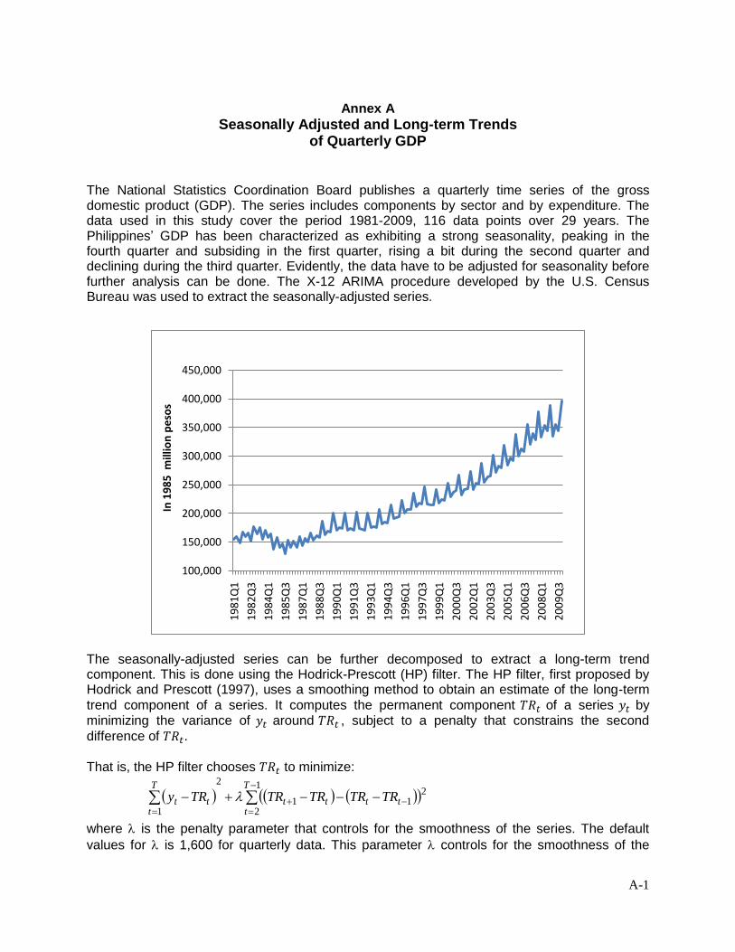
A-1

Annex A

Seasonally Adjusted and Long-term Trends of Quarterly GDP

The National Statistics Coordination Board publishes a quarterly time series of the gross domestic product (GDP). The series includes components by sector and by expenditure. The data used in this study cover the period 1981-2009, 116 data points over 29 years. The Philippines’ GDP has been characterized as exhibiting a strong seasonality, peaking in the fourth quarter and subsiding in the first quarter, rising a bit during the second quarter and declining during the third quarter. Evidently, the data have to be adjusted for seasonality before further analysis can be done. The X-12 ARIMA procedure developed by the U.S. Census Bureau was used to extract the seasonally-adjusted series.

The seasonally-adjusted series can be further decomposed to extract a long-term trend component. This is done using the Hodrick-Prescott (HP) filter. The HP filter, first proposed by Hodrick and Prescott (1997), uses a smoothing method to obtain an estimate of the long-term

trend component of a series. It computes the permanent component of a series by minimizing the variance of around , subject to a penalty that constrains the second

difference of .

That is, the HP filter chooses to minimize:

where is the penalty parameter that controls for the smoothness of the series. The default

values for is 1,600 for quarterly data. This parameter controls for the smoothness of the

1

2

211

2

1

T

ttttt

T

ttt TRTRTRTRTRy

100,000

150,000

200,000

250,000

300,000

350,000

400,000

450,000

19

81

Q1

19

82

Q3

19

84

Q1

19

85

Q3

19

87

Q1

19

88

Q3

19

90

Q1

19

91

Q3

19

93

Q1

19

94

Q3

19

96

Q1

19

97

Q3

19

99

Q1

20

00

Q3

20

02

Q1

20

03

Q3

20

05

Q1

20

06

Q3

20

08

Q1

20

09

Q3

In 1

98

5 m

illio

n p

eso

s

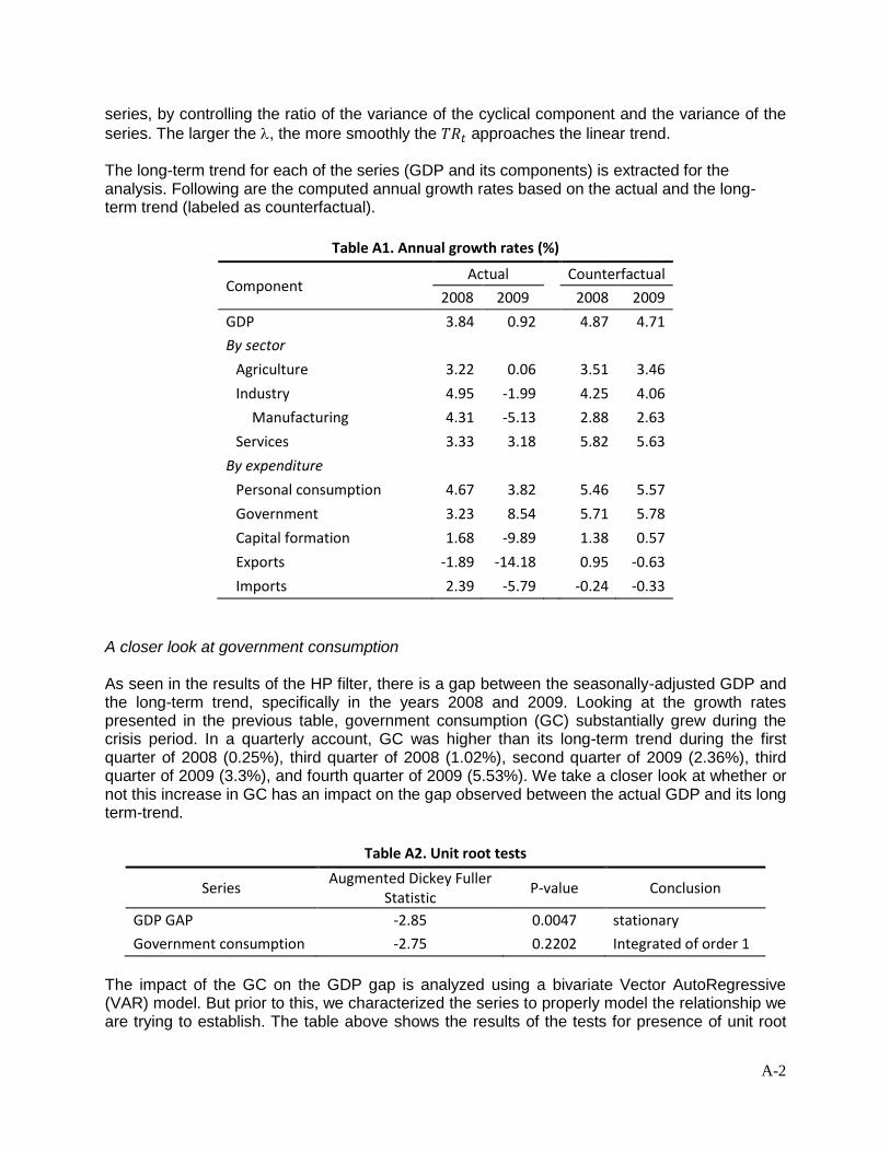
A-2

series, by controlling the ratio of the variance of the cyclical component and the variance of the

series. The larger the , the more smoothly the approaches the linear trend. The long-term trend for each of the series (GDP and its components) is extracted for the analysis. Following are the computed annual growth rates based on the actual and the long-term trend (labeled as counterfactual).

Table A1. Annual growth rates (%)

Component Actual Counterfactual

2008 2009 2008 2009

GDP 3.84 0.92 4.87 4.71

By sector

Agriculture 3.22 0.06 3.51 3.46

Industry 4.95 -1.99 4.25 4.06

Manufacturing 4.31 -5.13 2.88 2.63

Services 3.33 3.18 5.82 5.63

By expenditure

Personal consumption 4.67 3.82 5.46 5.57

Government 3.23 8.54 5.71 5.78

Capital formation 1.68 -9.89 1.38 0.57

Exports -1.89 -14.18 0.95 -0.63

Imports 2.39 -5.79 -0.24 -0.33

A closer look at government consumption As seen in the results of the HP filter, there is a gap between the seasonally-adjusted GDP and the long-term trend, specifically in the years 2008 and 2009. Looking at the growth rates presented in the previous table, government consumption (GC) substantially grew during the crisis period. In a quarterly account, GC was higher than its long-term trend during the first quarter of 2008 (0.25%), third quarter of 2008 (1.02%), second quarter of 2009 (2.36%), third quarter of 2009 (3.3%), and fourth quarter of 2009 (5.53%). We take a closer look at whether or not this increase in GC has an impact on the gap observed between the actual GDP and its long term-trend.

Table A2. Unit root tests

Series Augmented Dickey Fuller

Statistic P-value Conclusion

GDP GAP -2.85 0.0047 stationary

Government consumption -2.75 0.2202 Integrated of order 1

The impact of the GC on the GDP gap is analyzed using a bivariate Vector AutoRegressive (VAR) model. But prior to this, we characterized the series to properly model the relationship we are trying to establish. The table above shows the results of the tests for presence of unit root

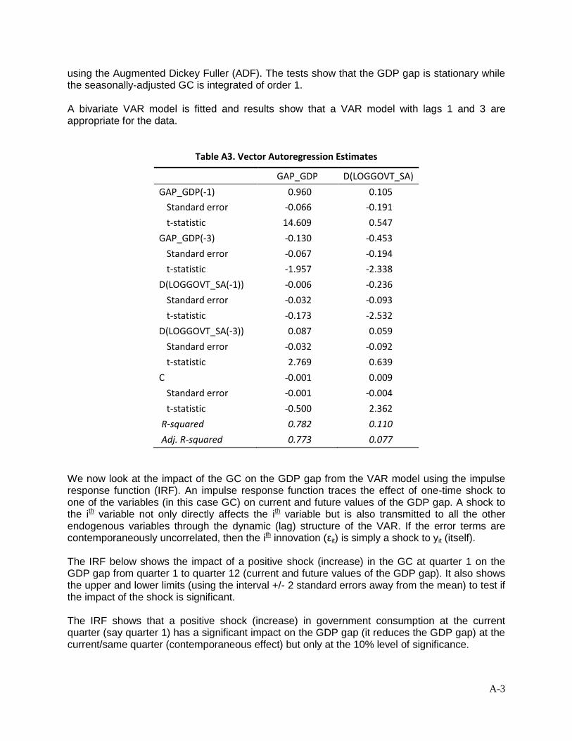
A-3

using the Augmented Dickey Fuller (ADF). The tests show that the GDP gap is stationary while the seasonally-adjusted GC is integrated of order 1. A bivariate VAR model is fitted and results show that a VAR model with lags 1 and 3 are appropriate for the data.

Table A3. Vector Autoregression Estimates

GAP_GDP D(LOGGOVT_SA)

GAP_GDP(-1) 0.960 0.105

Standard error -0.066 -0.191

t-statistic 14.609 0.547

GAP_GDP(-3) -0.130 -0.453

Standard error -0.067 -0.194

t-statistic -1.957 -2.338

D(LOGGOVT_SA(-1)) -0.006 -0.236

Standard error -0.032 -0.093

t-statistic -0.173 -2.532

D(LOGGOVT_SA(-3)) 0.087 0.059

Standard error -0.032 -0.092

t-statistic 2.769 0.639

C -0.001 0.009

Standard error -0.001 -0.004

t-statistic -0.500 2.362

R-squared 0.782 0.110

Adj. R-squared 0.773 0.077

We now look at the impact of the GC on the GDP gap from the VAR model using the impulse response function (IRF). An impulse response function traces the effect of one-time shock to one of the variables (in this case GC) on current and future values of the GDP gap. A shock to the ith variable not only directly affects the ith variable but is also transmitted to all the other endogenous variables through the dynamic (lag) structure of the VAR. If the error terms are contemporaneously uncorrelated, then the ith innovation (εit) is simply a shock to yit (itself). The IRF below shows the impact of a positive shock (increase) in the GC at quarter 1 on the GDP gap from quarter 1 to quarter 12 (current and future values of the GDP gap). It also shows the upper and lower limits (using the interval +/- 2 standard errors away from the mean) to test if the impact of the shock is significant. The IRF shows that a positive shock (increase) in government consumption at the current quarter (say quarter 1) has a significant impact on the GDP gap (it reduces the GDP gap) at the current/same quarter (contemporaneous effect) but only at the 10% level of significance.

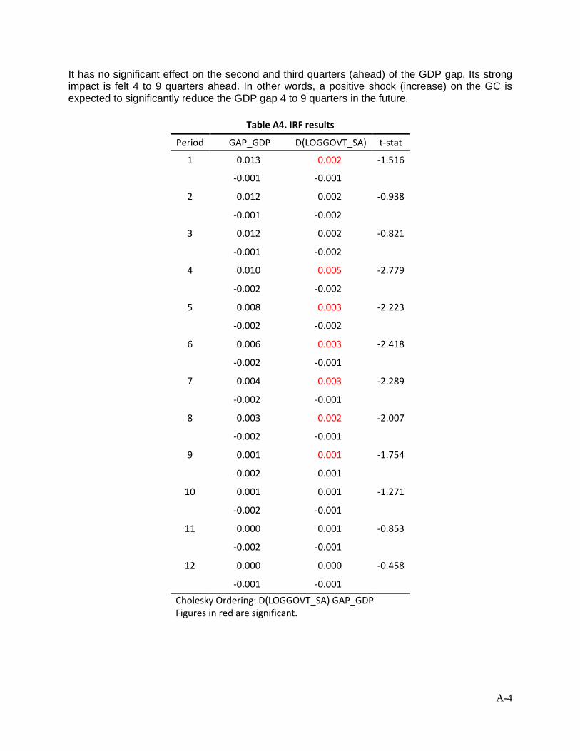
A-4

It has no significant effect on the second and third quarters (ahead) of the GDP gap. Its strong impact is felt 4 to 9 quarters ahead. In other words, a positive shock (increase) on the GC is expected to significantly reduce the GDP gap 4 to 9 quarters in the future.

Table A4. IRF results

Period GAP_GDP D(LOGGOVT_SA) t-stat

1 0.013 0.002 -1.516

-0.001 -0.001

2 0.012 0.002 -0.938

-0.001 -0.002

3 0.012 0.002 -0.821

-0.001 -0.002

4 0.010 0.005 -2.779

-0.002 -0.002

5 0.008 0.003 -2.223

-0.002 -0.002

6 0.006 0.003 -2.418

-0.002 -0.001

7 0.004 0.003 -2.289

-0.002 -0.001

8 0.003 0.002 -2.007

-0.002 -0.001

9 0.001 0.001 -1.754

-0.002 -0.001

10 0.001 0.001 -1.271

-0.002 -0.001

11 0.000 0.001 -0.853

-0.002 -0.001

12 0.000 0.000 -0.458

-0.001 -0.001

Cholesky Ordering: D(LOGGOVT_SA) GAP_GDP Figures in red are significant.