TACI: Taxonomy-Aware Catalog Integration - Stanford University

IEEE TRANSACTIONS ON KNOWLEDGE AND DATA ENGINEERING, VOL., NO., 2012 1

TACI: Taxonomy-Aware Catalog IntegrationPanagiotis Papadimitriou, Member, IEEE, Panayiotis Tsaparas, Member, IEEE,

Ariel Fuxman, Member, IEEE, Lise Getoor, Member, IEEE

Abstract—A fundamental data integration task faced by online commercial portals and commerce search engines is theintegration of products coming from multiple providers to their product catalogs. In this scenario, the commercial portal has itsown taxonomy (the “master taxonomy”), while each data provider organizes its products into a different taxonomy (the “providertaxonomy”). In this paper, we consider the problem of categorizing products from the data providers into the master taxonomy,while making use of the provider taxonomy information. Our approach is based on a taxonomy-aware processing step thatadjusts the results of a text-based classifier to ensure that products that are close together in the provider taxonomy remainclose in the master taxonomy. We formulate this intuition as a structured prediction optimization problem. To the best of ourknowledge, this is the first approach that leverages the structure of taxonomies in order to enhance catalog integration. Wepropose algorithms that are scalable and thus applicable to the large datasets that are typical on the Web. We evaluate ouralgorithms on real-world data and we show that taxonomy-aware classification provides a significant improvement over existingapproaches.

Index Terms—catalog integration, classification, data mining, taxonomies.

F

1 INTRODUCTION

An increasing number of Web portals provide auser experience centered around online shopping.This includes e-commerce sites such as Amazon andShopping.com, and commerce search engines such asGoogle Product Search and Bing Shopping. A fun-damental data integration task faced by these com-mercial portals is the integration of data coming frommultiple data providers into a single product catalog.An important step in this process is product categoriza-tion. All portals maintain a comprehensive “master”taxonomy for organizing their products, which is usedboth for browsing and searching purposes. As newproducts arrive from different providers they need tobe assigned to the appropriate category in the mastertaxonomy in order to be accessible to the users. Atthe web scale, it is impractical to assume that dataproviders will manually assign all the products fromtheir catalog to the appropriate category in the mastertaxonomy. Thus, we need automated techniques forcategorizing products coming from the data providersinto the master taxonomy.

An important observation in this scenario is that

• P. Papadimitriou is with oDesk Research, Redwood City, CA 94063,USA. Part of the work done while interning at Microsoft Research.E-mail: [email protected].

• P. Tsaparas is with University of Ioannina, Ioannina, Greece. Workdone while working at Microsoft Research.E-mail: [email protected].

• A. Fuxman is with Microsoft Research Search Labs, Mountain View,CA, 94043.E-mail: [email protected].

• L. Getoor is with University of Maryland at College Park, CollegePark, MD 20742. Work done while visiting Microsoft Research.E-mail: [email protected].

Manuscript received July 21, 2011; revised January 10, 2012; acceptedFebruary 17, 2012.

the data providers do have their own taxonomy (the“provider taxonomy”), and their products are alreadyassociated with a provider taxonomy category. Theprovider taxonomy may be different from the mastertaxonomy, but in most cases, there is still a powerfulsignal coming from the provider classification. Intu-itively, products that are in nearby categories in theprovider taxonomy, should be classified into nearbycategories in the master taxonomy.

To illustrate this point, consider the example inFigure 1. The provider taxonomy is an excerpt fromthe taxonomy used by Amazon, and the master tax-onomy is an excerpt from the taxonomy used byBing Shopping. Now, given a product tagged witha category from Amazon’s (provider) taxonomy, wewant to categorize it in the Bing Shopping (master)taxonomy. Suppose we are given the product “BossAudio Systems CH6530” from the category Electron-ics/Car Electronics/Car Audio & Video/Car Speakers/CoaxialSpeakers in the Amazon taxonomy. If we use a text-based classifier to categorize this product into theBing taxonomy, it is unclear whether this productshould be classified into Electronics/Car Electronics/CarAudio/Car Speakers or Electronics/Home Audio/Speakers.If we know that most of the products in the Car Speak-ers/Coaxial Speakers Amazon category are categorizedto the Car Speakers category in Bing, then we canconclude that most likely the new product should alsobe classified in Car Speakers.

However, for most products in the Electronics/CarElectronics/Car Audio & Video/Car Speakers/Coaxial Speak-ers from the Amazon taxonomy, the classifier is actu-ally unable to decide if they should be classified inCar Speakers, or Audio Speakers. Therefore, we cannotuse the categorization of the products in the samecategory as the new product to guide as for the correct


Provider Taxonomy (Amazon)

All

Electronics Software

Computers-Accessories

Car Electronics

Car, Audio & Video

GPS & Navigation

Satellite Radio

Car Speakers

Channel Speakers

Coaxial Speakers

All

Electronics Software

Home AudioCar

Electronics

Car VideoCar Audio

Car Speakers

Car Amplifiers

Computing

SpeakersRadios

Boss Audio Systems CH6530Chaos Series 6.5 inch 3-way speaker, 300W Peak Power

Master Taxonomy(Bing)

Fig. 1. A simple catalog integration example.

decision. In this case, the taxonomy information canhelp to determine the correct categorization. As we goup the taxonomy tree of the Amazon taxonomy, weobserve that many more products in the Car Audio &Video Amazon category are classified to the Car Audiomaster category, as opposed to the Home Audio mastercategory. Using this information we can conclude thatmost likely the products from the Electronics/Car Elec-tronics/Car Audio & Video/Car Speakers/Coaxial Speakerscategory should be mapped to Electronics/Car Electron-ics/Car Audio/Car Speakers rather than Electronics/HomeAudio/Speakers.

In this work, we propose techniques that leveragethe intuition described above. We show how we canuse the taxonomy information in order to “adjust”the results of a text-based classifier, and improve theproduct categorization accuracy. The key contributionof our work is that we make use of the structureof the master and provider taxonomies in order toachieve this goal, exploiting the relationships betweendifferent categories in the taxonomy, rather than rely-ing on the category membership information of theproducts. In the example we described above, whenthe text-based classifier fails to give a clear classifi-cation of the new product, the category-membershipinformation of the product in the provider taxonomydoes not provide any additional help since there isno clear mapping between categories at the leaf level.However, there is a strong signal about the correctclassification coming from mappings at higher levelsof the taxonomies. Using the taxonomy structure, wecan propagate this information to the lower levelsof the taxonomy, and assign the correct leaf-levelcategory to the new product.

The idea of using the “structure” of the data to en-hance classification underlies many structured predic-tion approaches, and has been shown to work well inother areas such as computer vision [4] and NLP [3].The general principle is that we can improve theaccuracy of classification by making use of relation-ships between the items that are classified. However,previous approaches for catalog integration [1], [28]

ignore possible relationships among the taxonomycategories, essentially treating the taxonomy as a flatcollection of classes. In contrast, we exploit the fullstructure of the taxonomy, defining relationships be-tween items that belong to different categories, basedon the relationship of the categories in the taxonomytree. Furthermore, most of the previous approachessuffer from scalability issues due to the large numberof pairwise relationships that need to be considered.For the catalog integration problem, where we areinterested in categorizing hundreds of thousands, ormillions of products, such solutions are impractical.In our work, we carefully prune the relationships weconsider for the classification of an item to obtain ascalable linear-time algorithm.

Contributions. In this work we make the followingcontributions:

1) We formulate the taxonomy-aware catalog in-tegration problem as a structured predictionproblem. To the best of our knowledge, this isthe first approach that leverages the structureof the taxonomies in order to enhance catalogintegration.

2) We present techniques that have linear runningtime with respect to the input data and are appli-cable to large-scale catalogs. This is in contrast toother structured classification algorithms in theliterature which face challenges scaling to largedatasets due to quadratic complexity.

3) We perform an extensive empirical evaluationof our algorithms on real-world data. We showthat taxonomy-aware classification provides asignificant improvement in accuracy over exist-ing state-of-the-art classifiers.

The rest of the paper is organized as follows. InSection 2 we formally define the catalog integrationproblem. In Section 3 we present our approach, andin Section 4 an efficient algorithm for our formulation.Section 5 contains the experimental evaluation of ourapproach. In Section 6 we present the related work,and in Section 7 we give our concluding remarks.


2 PROBLEM DEFINITION

We now introduce some basic terminology, and for-mulate the taxonomy-aware catalog integration problem.

A product x is an item that can be bought at acommercial portal. Each product has a textual rep-resentation that consists of a name (a short sentencedescribing the product), and possibly a set of attribute-value pairs. For example, Figure 1 shows a productwhose name is “Boss Audio Systems CH6530”, and hasalso a description attribute with value “Chaos Series6.5-Inch 3-Way Speaker, 300W peak power”. Note thatthe name and the attributes of a product may varyacross providers. For example, another provider mayuse the name “Boss CH6530 Speakers” for the same carspeakers, and have no description, or other attributesassociated with the product.

A product taxonomy G = (Cg, Eg) is a directedacyclic graph whose nodes Cg represent the set ofpossible categories into which products are organized.Each graph edge (c1, c2) ∈ Eg represents a subsumption(i.e., an “is-a”) relationship between two categoriesc1 and c2. For example, in the master taxonomyof Figure 1, category Electronics subsumes categoryCar Electronics. Typically, the taxonomy structure is arooted tree, where each category (excluding the root)has a single parent. A directed acyclic graph (DAG)is also possible, where a category may have multipleparents. We make the assumption that a taxonomyis a tree with a single root, thus imposing a clearhierarchical structure. The distance of a category fromthe root is the depth of the category in the taxonomy.For example, in the Master taxonomy of Figure 1,category Electronics has depth 1, while Car Electronicshas depth 2.

A product catalog K = (P,G, v) is a taxonomy Gpopulated with a set of products P as defined by themapping function v : P → Cg that maps each productin P to a category in Cg . Abusing the notation, wewill use v to denote the output vector of function v

on P , that is, v ∈ C |P |g , and element vx of the vectorv denotes the category of product x in taxonomy G.Since v is a function, we assume that each product isassociated to exactly one category, although our workcan also be applied to cases where this assumptiondoes not hold.

In the taxonomy-aware catalog integration problem,we are given a source catalog Ks = (Ps, S, s) thatcorresponds to some provider’s catalog defined overthe source taxonomy S = (Cs, Es), and a target (ormaster) catalog Kt = (Pt, T, t) that corresponds to thecatalog of the commercial portal defined over thetarget (master) taxonomy T = (Ct, Et). The goal is tolearn a cross-catalog labeling function ` : Ps → Ct thatmaps products of the source catalog to the categoriesof the target catalog taxonomy. Similar to before, weabuse the notation and we use ` ∈ C |Ps|t to denote thelabeling vector, where the entry `x of the vector is the

assigned category of product x ∈ Ps in taxonomy T .We can now define our problem abstractly as fol-

lows:Definition 1 (Taxonomy-Aware Catalog Integration):

Given a source catalog Ks and a target catalog Kt, usea taxonomy-aware process fT to learn a cross-cataloglabeling function ` = fT (Ks,Kt).

The key novelty in our approach is that the learningprocess fT that produces labeling vector ` makes useof the full taxonomy structure of the taxonomies Sand T in order to define relationships between prod-ucts in the source and target catalog, and guide theclassification process. Previous approaches [1] haveexploited the category assignments s, and t, but notthe structure of the taxonomies S and T . In the nextSection we describe how to formulate the process fTas a combinatorial optimization problem.

3 TAXONOMY-AWARE CLASSIFICATION

At a high level we can describe our approach totaxonomy-aware classification as a two-step process.First, each product is classified using a base classifierthat is not aware of the taxonomies. We call this thebase classification step. Then, we use the structure ofthe source and target taxonomies in order to adjustthe output of the base classifier, and produce a finalclassification. We call this the taxonomy-aware process-ing step. We now discuss these two steps in detail.

3.1 The Base Classification StepIn the base classification step, we classify the productsbased solely on their textual representation. For thispurpose, we train a text-based classifier using stan-dard supervised machine learning techniques. In thispaper, we consider Naive Bayes, and Logistic Regres-sion [18], but any other machine learning techniquecould be used. We use a subset of the target catalogas the training set. This provides us with examplesof products labeled with categories of the target tax-onomy. The features of the classifier are extractedfrom the textual product representations. Note that attraining time we have no knowledge of the providers’catalogs, and we make no use of the structure of thetarget taxonomy.

Let b denote the classification model we obtain aftertraining. Given an product x ∈ Ps from the providercatalog we apply the classifier b on the textual represen-tation of the product, as this appears in the provider’scatalog. In our example in Figure 1 the features areextracted from the text “Boss Audio Systems CH6530,Chaos Series 6.5-Inch 3-Way Speaker, 300W peak power”.The output of the base classification step is a proba-bility distribution Prb[τ |x] over all target categoriesτ ∈ Ct for each product x ∈ Ps. The probabilityPrb[τ |x] provides an estimate of the likelihood thatproduct x belongs to category τ , and the confidencethat the classifier has for this assignment.


We stress again that during the base classificationstep we do not make use of any knowledge aboutthe target or source taxonomy, either during training,or during the application of the classifier. This refersto both the structure of the taxonomy, as well as thenames of the categories. It is possible for the classifierto try to match the names of the categories betweenthe source and target taxonomies. However, this en-tails the danger of over-fitting, and also as we haveobserved, category names often vary significantly be-tween providers (e.g., Cameras v.s. Photography).

3.2 The Taxonomy-Aware Processing Step

The intuition behind the taxonomy-aware processingstep is that the target categories assigned by thebase classification step can be adjusted by taking intoaccount the relationships of the products in the sourceand target taxonomies. The goal of the taxonomy-aware processing is to assign categories in the targettaxonomy to the products coming from the provider’scatalog, such that the assignments respect the deci-sions of the base classifier, while at the same timethey preserve the relative relationships of the productsin the source taxonomy. We will now show how thetaxonomy-aware processing step can be defined asan optimization problem, and discuss the differentparameters of the problem.

3.2.1 The Optimization ProblemFormally, we define taxonomy-aware processing as anoptimization problem, where given a source catalogKs, and a target catalog Kt, the objective is to finda labeling vector ` that minimizes the following costfunction:

COST(Ks,Kt, `) =(1− γ)∑x∈Ps

ACOST(x, `x)

+ γ∑

x,y∈Ps

SCOST(x, y, `x, `y) (1)

The taxonomy-aware process fT is the algorithm thatfinds the labeling ` that minimizes the cost function:

fT (Ks,Kt) = arg min`

COST(Ks,Kt, `).

The first term of the cost function, ACOST, is theassignment cost which penalizes classifications thatdiffer from the ones chosen by the base classifier. Wedefine the assignment cost in Section 3.2.2. The secondterm, SCOST is the separation cost which penalizesclassifications that place products that are close in thesource taxonomy to distant categories in the targettaxonomy (or vice-versa). We introduce the separationcost in Section 3.2.3 and we discuss it in detail in Ap-pendix A. The parameter γ (also called regularizationparameter) balances between the two costs. Note thatan optimal classification ` may assign a product x to atarget category `x that is different from the one chosen

TABLE 1Category similarity and penalty functions used in

separation cost.

Category similarity functions: simG(c1, c2)

Shortest-Path similarity 2−hops(c1,c2)

LCA similarity 1− 2−depth(lca(c1,c2))

Cosine similarity 1+depth(lca(c1,c2))√1+depth(c1)

√1+depth(c2)

Penalty functions: SCOST(sx, sy , `x, `y)

Absolute difference |simS(sx, sy)− simT (`x, `y)|Multiplicative simS(sx, sy)(1− simT (`x, `y))

by the base classifier, if the neighboring products of xin the source taxonomy are assigned target categoriesthat are close to category `x in the target taxonomy. Inthis way, we are getting signal both from the productrepresentation (assignment cost) and from the sourcecategories and taxonomy structure (separation cost).

3.2.2 Assignment CostWe use the probabilities of the base classifier to definethe assignment cost function ACOST: Ps × Ct → R+.For a product x the cost of classifying product x totarget category `x is defined as follows:

ACOST(x, `x) = 1− Prb[`x|x] (2)

This definition penalizes the classification of productx to a category `x for which the base classifier yieldssmall probability estimates. On the other hand, theassignment cost is small if product x is assigned toa category for which the base classifier assigns highprobability.

3.2.3 Separation CostThe separation cost function SCOST : P 2

s ×C2t → R+ is

defined over a pair of products x, y ∈ Ps that we wantto classify, and a pair of categories `x, `y ∈ Ct that arecandidate target categories for x and y respectively.Intuitively, it captures the cost of separating productsx and y to target categories `x and `y . The separationcost should be high if products x and y belong tocategories sx, sy that are close in the source taxonomy,and which are assigned classes `x, `y that are distantin the target taxonomy.

To formally define this intuition, we need a defini-tion of similarity between two categories in a taxon-omy. For a given taxonomy G = (C,E) a similarityfunction simG : C × C → [0, 1] returns a value in[0, 1] for any two categories c1, c2 ∈ C, where 1 meansthat categories c1 and c2 are identical and 0 meansthat they are completely dissimilar. A meaningfulsimilarity definition should satisfy the intuition thattwo categories that are close in the taxonomy tree aremore similar than two categories that are far apart.For example, two categories that have a commonparent are more similar than two categories that havedifferent parents and a common grandparent.

With the notion of category similarity at hand, wenow define the separation cost as a function of the


similarity simS(sx, sy) between categories sx and sy ofx and y in the source taxonomy S and the similaritysimT (`x, `y) between `x and `y in the target taxonomyT , that is,

SCOST(x, y, `x, `y) = δ (simS(sx, sy), simT (`x, `y)) (3)

where δ is a penalty function that yields high valuesif the similarity simS(sx, sy) of the source categoriesis high, while the similarity simT (`x, `y) is low, orvice versa. An example of the penalty function δ isthe absolute difference of the two similarity values.Intuitively, we want the relative position of assignedcategories of two products in the target taxonomy tobe similar to the relative position of the categories inthe source taxonomy.

Depending on the choice of the penalty and simi-larity functions, we obtain different definitions for theseparation cost. The similarity and penalty functionsthat we consider in this work are listed in Table 1, to-gether with their mathematical definition. We discussthe definitions in detail in Appendix A.

Note that as defined in Equation 3, for a givenchoice of the penalty function δ, the separation cost isfully defined by the tuple (sx, sy, `x, `y), and it doesnot depend on the identities of the individual prod-ucts x and y. We can thus write SCOST(sx, sy, `x, `y)to denote the separation cost SCOST(x, y, `x, `y). Thatis, we can define the function SCOST : C2

s ×C2t → R+

over pairs of source and target categories.The key observation is that all pairs of products

x, y such that sx = σ and `x = τ , and sy = σ and`y = τ , for some σ, σ ∈ Cs, and τ, τ ∈ Ct havethe same separation cost SCOST(σ, σ, τ, τ). That is, theseparation cost is the same for all pairs of productsx, y that that come from source categories σ and σrespectively, and are assigned to target categories τand τ respectively. If n(σ, τ) denotes the number ofproducts from σ that are assigned to τ , accordingto some labeling `, then, there are n(σ, τ) · n(σ, τ)such pairs of products, and each one will contributeSCOST(σ, σ, τ, τ) to the separation cost. Then, we canwrite the separation cost in Equation 1 as follows:∑

x,y∈Ps

SCOST(x, y, `x, `y) (4)

=∑

σ,σ∈Cs

∑τ,τ∈Ct

SCOST(σ, σ, τ, τ)n(σ, τ)n(σ, τ)

Note that the sum in Equation 4 is now expressedover pairs of source categories and pairs of targetcategories, rather than pairs of products. We leveragethis observation for the efficient computation of theseparation cost that we present in Section 4.

Although we do not discuss it further in this pa-per, we can modify Equation 3 to handle multi-classclassification of products in the source taxonomy. Ifx and y are classified in more than one categoriesin the source taxonomy then sx and sy are now sets

of categories, rather than single categories. Given asimilarity measure between the set members thereare different ways for defining the similarity betweensets that we can employ. One possibility is to use themaximum similarity of any pair of elements betweenthe two sets. The intuition for such a choice is thatif two products x and y appear in close-by categoriesin a taxonomy then they are similar, even if they alsoappear in some distant categories.

4 THE TACI ALGORITHM

The optimization problem in Section 3.2.1 is closelyrelated to a variety of optimization problems suchas the metric labeling problem [12], or structured pre-diction problems [3]. These problems are known tobe NP-hard when asking for a hard labeling of thedata. For certain variants there are approximationalgorithms [5], [6], [12], [23]. Our problem can beformulated as an Integer Linear Program (ILP) or aQuadratic Integer Program (QIP), however the num-ber of variables is proportional to the number ofproducts in the source catalog, which is prohibitivelylarge. To the best of our knowledge, none of thesolutions that have been proposed are applicable toweb-scale classification problems, where the numberof products to be classified can be in the order ofhundreds of thousands, or millions.

In this section, we present a scalable algorithm forthe taxonomy-aware classification step that scales upto large datasets. Although we present our techniquewith respect to our specific problem, the methodol-ogy that we propose can be applied to other struc-tured prediction problems in order to deal with thequadratic number of pairwise relationships that needto be considered. To aid the presentation, we refer thereader to Table 2 which explains the main terminologyand symbols that we will use in this section.

4.1 Search Space PruningWe now present a heuristic for efficiently performingthe taxonomy-aware calibration step. The idea is tojudiciously fix the category for some of the products inthe source catalog in order to obtain a landscape of themappings between the two taxonomies. We then treateach of the open (non-fixed) products independentlymaking use of Equation 4 to efficiently compute theseparation cost.

We identify the products whose assigned class canbe fixed using the output of the base classifier. Theintuition is that if the base classifier is sufficiently“confident” about the top category of a source prod-uct, then it is likely to be making the correct pre-diction. However, if it is not confident about thecategory (low probability estimate), it might not bepredicting the right category and therefore we shouldconsider adjusting the assignment at the taxonomy-aware calibration step.


TABLE 2Algorithm terminology chart.

Generic termsS, T source and target taxonomiesCs, Ct sets of source and target taxonomy categoriesσ, τ denote a source and target taxonomy categoryPs set of source catalog products

Algorithm Parametersk number of top categories to consider as candidatesθ probability threshold for fixing the categoryγ regularization parameter between assignment and

separation costVariables used in TACI algorithm

Prb[τ |x] probability of category τ for product x output bybase classifier b

Fθ products whose category is fixedOθ open products whose category is not fixed

h(σ, τ) separation cost for product coming from categoryσ and assigned to category τ

Ψ cache for h(σ, τ) valuesHθ,k source-target category pairs for which we need to

compute the separation cost h

Let θ ∈ [0, 1] be a threshold value that defineswhen the category probability estimate returned bythe base classifier is large enough so that the predictedcategory is likely to be correct. Let Fθ be the subsetof products that pass the threshold, that is:

Fθ = {x ∈ Ps|maxτ∈Ct

Prb[τ |x] ≥ θ}. (5)

For the products in Fθ we trust the prediction of theclassifier, and we fix their labeling to the most likelybase classifier output. That is, for all x ∈ Fθ

`x = arg maxτ∈Ct

Prb[τ |x]. (6)

Let Oθ = Ps \ Fθ denote the products whose clas-sification remains open. We treat each open productx ∈ Oθ independently, and we compute a separationcost for x only with respect to the fixed products inFθ. If sx is the source category of x, and tx is acandidate target category, then the separation cost forthis source-target pair is defined as follows:

h(sx, `x) =∑y∈Fθ

SCOST(x, y, tx, `y).

Using Equation 4 we can rewrite h(sx, tx) as:

h(sx, tx) =∑

σ∈S,τ∈T

SCOST(sx, σ, tx, τ)n(sx, tx)n(σ, τ) (7)

where n(σ, τ) is the number of products in Fθ thatbelong in category σ in S and are assigned to categoryτ in T . Therefore, by fixing the labeling of the productsin Fθ we have effectively achieved the following: first,we have created a set of “anchors” against which wecompute the separation cost for a new open product;second, the n(σ, τ) values, define a mapping betweenthe source and target taxonomies. This mapping isused to compute the separation cost, and guide thecategorization of new open products.

To further speed-up the taxonomy-aware classifi-cation step, we also reduce the space of candidatesource-target pairs. For an open product x ∈ Oθ, let

TOPk(x) denote the top-k candidate target categorieswith respect to the probability estimates Prb[τ |x] ofthe base classifier. We reduce the search space by con-sidering only these k target categories as candidatesfor product x. As we discuss in Section 4.3, restrictingourselves to the top-k categories does not significantlylimit our maximum achievable accuracy.

We use Hθ,k to denote the set of candidate source-target pairs for which we need to compute the sepa-ration cost h:

Hθ,k = {(sx, τ) : x ∈ Oθ, τ ∈ TOPk(x)}.

From Equation 7 it follows that the separation cost forthe pairs in Hθ,k can be computed using the mappingsdefined by the products in Fθ, and it is independentof the products in Oθ. Therefore, for each candidatesource-target category pair (σ, τ), we need to computethe separation cost h(σ, τ) only once, and store thevalue for future use. We describe the algorithm indetail in the next section.

4.2 Taxonomy-Aware AlgorithmAlgorithm 1 describes the Taxonomy Aware CatalogIntegration algorithm (henceforth referred to as theTACI algorithm). The algorithm assumes the existenceof a base classifier trained on data from the targetcatalog. The input to the algorithm consists of asource catalog and a target taxonomy, as well as theparameters θ, k, and γ. The output of the algorithmis a labeling ` for the products in the source catalog.

In the loop of Lines 2-9, the algorithm appliesthe base classifier to each product. Based on thebase classifier output probabilities, the algorithm ei-ther classifies the product to the top category givenby the base classifier (Lines 4-6), or it leaves itsclassification open and stores the top k categories,sorted by probability (Lines 7-9). Given the set ofopen products Oθ, and their top-k candidate targetcategories the algorithm computes the set of candidatesource-category pairs Hθ,k (Line 10). In the loop ofLines 12-13 the algorithm computes the separationcosts for all of the candidate pairs (σ, τ) ∈ Hθ,k, andstores them in a hash table Ψ. Note that for eachsource-target pair we compute the value of h onlyonce, and we never compute a separation cost thatwe will not use later on. In the loop of lines 14-15the algorithm classifies the open products in Oθ. Aproduct x ∈ Oθ is assigned to the category `x amongthe top-k categories in TOPk(x) that minimizes theobjective function.

We now provide an analysis of the running timeof the algorithm. The first loop in Lines 2-9 iteratesover the set Ps of all products in the source taxonomy,and requires O(|Ct|) time to process each product,where |Ct| is the number of categories in the targettaxonomy. Hence, the running time of the first loop isO(|Ps||Ct|). The set of candidate pairs Hθ,k has size at


Algorithm 1 TACI AlgorithmInput: source catalog Ks, target taxonomy T , base classifier

b, and parameters θ,k, and γ.Output: a labeling vector `

1: Fs ← ∅2: for all x ∈ Ps do3: τ∗ ← arg maxτ∈Ct Prb[τ |x]4: if Prb[τ∗|x] ≥ θ then5: `x ← τ∗

6: Fθ ← Fθ ∪ {x}7: else8: Oθ ← Oθ ∪ {x}9: Compute TOPk(x)

10: Compute candidate pairs Hθ,k11: Initialize hash table Ψ to empty12: for all (σ, τ) ∈ Hθ,k do13: Ψ[(σ, τ)] = h(σ, τ)

14: for all x ∈ Oθ do15: `x ← argmin

τ∈TOPk(x)

{(1− γ)ACOST(x, τ) + γΨ[(sx, τ)]}

most |Cs||Ct|, and thus the computation of the candi-date pairs at Line 10, has cost at most O(|Cs||Ct|).However, we expect this to be significantly lower,since for each product we are only considering thetop-k categories, and it is unlikely that all possiblepairs of categories will occur in practice. In the loopof lines 12-13, the algorithm computes the separationcost h(σ, τ) for all candidate pairs in Hθ,k. The costof calculating h(σ, τ) is O(|Cs||Ct|), so the worst caserunning time of the loop is O(|Cs|2|Ct|2). Again, weexpect this to be smaller in practice, since the sizeof the candidate set is likely to be smaller. The loopin Lines 14-15 now just sums up the precomputedcosts, for the open products in Oθ for each one ofthe top-k candidate categories. The processing time isO(k|Ps|). Thus, the total running time of Algorithm 1is O(|Ps||Ct|)+O(|Cs|2|Ct|2)+O(k|Ps|), which is linearwith respect to the number of products |Ps| in thesource catalog.

4.3 Parameter Calibration

The tuning of the parameters k, γ and θ is importantfor the performance of our algorithm. Similarly toother works [1], [28], we assume the existence ofa validation set on which we tune the parameters.The validation set consists of products that are cross-labeled in both the source and the target taxonomy.To obtain such a set, we can either automaticallymatch source to master taxonomy products usingsome universal unique identifier such as the ISBN forbooks, or manually label some products of the sourcetaxonomy if such an identifier does not exist. In bothcases, it is assumed that the obtained validation setis too small to be used for the base classifier trainingthat involves tens of thousands of features, while itis big enough to tune few parameters of the TACIalgorithm.

The calibration of the parameters of the algorithmworks as follows. First, we run the base classifier b onthe products of the validation set, and for each prod-uct x we obtain a probability distribution Prb[τ |x].The first parameter we set is parameter k, such thatthe accuracy of the classifier over the top-k categoriesis high. The details are described below. Then wetune the parameters θ and γ. We consider a set{θ1, ..., θNθ} of candidate values selected as describedbelow. For each candidate parameter θi we find the“optimal” parameter γ such that the accuracy of theTACI algorithm on the validation set is maximized.The algorithm for estimating γ is described below. Weoutput the pair of parameters θ, γ that achieve themaximum accuracy. We note that all parameters areselected such as to maximize the accuracy of the TACIalgorithm on the validation set. Since the productson the validation set are cross-labeled we know thetrue labeling and we can compute the accuracy. Toavoid overfitting, when tuning the parameters θ andγ we do not update them unless we have a significantimprovement in the accuracy (0.1% of the previousvalue in our experiments).

Tuning Parameter k: we set the parameter k, suchthat the accuracy of the base classifier over the top-kresults (i.e., the fraction of times that the true categoryis contained in the top-k results) is above a certainthreshold (99% in our experiments), or k reachesa predefined maximum (20 in our experiments). Inthis way we guarantee that the TACI algorithm canachieve accuracy up to 99%.

Tuning Parameter θ: The parameter θ determines theanchor set Fθ: the products in Fθ should have highclassification accuracy, and at the same time capturethe true mappings between the source and targettaxonomies. The first requirement does not necessarilyimply the second, and thus we cannot set the thresh-old θ in the same way we did for k. We thus performa linear search for Nθ different values, and we selectthe one for which the calibration step gives the bestaccuracy. We judiciously select the candidate valuesfor θ using the probabilities output by base classifierto guide our choice. Let π∗x = Prb[τ

∗|x] denote theprobability of the most likely category of product x.We sort the probabilities π∗x and we select Nθ values,evenly spaced, as the candidate θ values. Thus, thechoice of the candidate values controls the fractionof products in the validation set that are below thethreshold: this is the set of products for which werun the taxonomy-aware step. This way we can focuson the appropriate range of candidate values.

In our experiments we used Nθ = 40 differentvalues that divide the base classifier probabilities in 40equally sized buckets. For example, if the validationset has 4000 products, then each interval [θi, θi+1) con-tains 100 products, that is, 2.5% of the total products.Furthermore, for the θi candidate value there are 100i


products that have probability π∗x ≤ θi for which werun the taxonomy-aware processing step.

Tuning Parameter γ: The parameter γ is importantsince it controls the effect of the taxonomy signal onthe classification. If the taxonomy provides a mislead-ing signal, then we need to minimize its contribu-tion to the optimization problem. We determine theparameter γ by making use of the assignment andseparation costs over the validation set, and findingthe value of γ that gives the best accuracy. For agiven product x in the validation set, let τ1, ..., τk bethe set of candidate target categories in TOPk(x), andlet τ∗ denote the correct category for x. Note thatτ∗ may not be one of the categories in TOPk(x). Foreach target category τi we can compute an assignmentcost ηi and a separation cost ζi. For a given valueof the parameter γ the cost of assigning x to thiscategory is ci = (1−γ)ηi+γζi. The item x will receivethe correct category τ∗, if τ∗ ∈ TOPk(x), and for allτi ∈ TOPk(x), c∗ ≤ ci. In this case, the correct categoryhas the minimum cost, and it will be selected by ouralgorithm. We want to find a value for γ that ensuresthat the above requirement is satisfied for as manyproducts in the validation set as possible.

The algorithm proceeds as follows. For each candi-date target category τi of product x we find the rangeof values for γ that satisfy the inequality:

(1− γ)η∗ + γζ∗ ≤ (1− γ)ηi + γiζ ,

where η∗ and ζ∗ denote the assignment and sepa-ration cost for the correct category τ∗. This is therange of values of γ for which the correct categoryτ∗ is selected over τi. If the interval [lx, ux] is theintersection of the ranges of values for all τi, then forany γ in this interval the correct category τ∗ is selectedover all categories in TOPk(x). If this interval is empty,or it does not intersect with [0, 1] (e.g., it is negative)then we discard item x since there is no value of γ forwhich we can assign x the correct category. Otherwise,any value in the interval [lx, ux] can be used as the γvalue. In this case we say that the interval satisfiesproduct x.

After processing all products, we obtain a set ofintervals, one for each product that was not discarded.For any value γ ∈ [0, 1], the number of intervalsin which it is contained is the number of productsit satisfies. Intersecting all the intervals we find therange of values [γl, γu] that satisfies the maximumnumber of products. We return the mean of theinterval γ = (γl + γu)/2 as the final value for theregularization parameter.

5 EXPERIMENTAL EVALUATION

In this section, we present the experimental evaluationof our approach. The main goals of this evaluationare the following: (1) to show the benefits of ourtaxonomy-aware calibration step and compare the

taxonomy-aware algorithm against other catalog in-tegration approaches (Section 5.2); (2) to evaluate thedifferent cost and similarity functions we consider(Section 5.3); and (3) to study the running time ofour algorithm (Section 5.4), and the sensitivity toparameter values (Section 5.5).

5.1 Experimental SetupDatasets. We use as master catalog the catalog of BingShopping, which aggregates data feeds from retailers,distributors, resellers, and other commercial portals.We consider three providers: Amazon, Etilize, andPricegrabber. The Amazon source catalog contains65, 512 products; the Etilize catalog has 136, 876 prod-ucts; and the Pricegrabber catalog consists of 544, 898products.

In all the experiments, we consider a target tax-onomy that consists of all the categories in BingShopping taxonomy that are related to consumer elec-tronics (all of the dataset products come from such cat-egories). The resulting taxonomy has 297 categories.There are 37 internal nodes, and 260 leaf nodes. Theheight of the tree is 4 and the average branchingfactor is 8.2. As source taxonomies, we use taxonomiesfrom the Amazon, Etilize and Pricegrabber providers,restricted to the consumer electronics domain. In thecase of Etilize, the taxonomy has 523 nodes, of which94 are internal nodes, and 429 are leaf nodes. Thetaxonomy tree has height 5, and an average branchingfactor of 5.6. The Pricegrabber taxonomy has 1001nodes, 211 of which are internal nodes and 790 areleaf nodes. Pricegrabber taxonomy has height 3 andaverage branching factor is 4.8. Amazon has 1788nodes in total, 1312 of which are leaves and 476 areinternal nodes. The height of the taxonomy is 7, andthe average branching factor is 3.8.

An important observation regarding the datasetsis the skewed category distribution over productsin all of the taxonomies. For example, the mastertaxonomy with all of the dataset products has fivecategories with more than 50K products each, whileit has approximately 70 categories with less than 500products. We can make similar observations for thesource taxonomies. The skewed category distributionover classified objects has also been observed in otherlarge web taxonomies [16]. This observation justifiesthe normalization step that we use in Section A.3.

Ground truth. The ground truth is the true labeling ofthe products in the provider catalog with categoriesfrom the master taxonomy. We obtained the groundtruth as follows: the Etilize products were manuallylabeled by human experts; the Pricegrabber productswere assigned a category from the master taxonomyby applying rules developed by domain experts; theAmazon products were associated to products in themaster catalog via universal identifiers (e.g., ASINand UPC numbers), and then they were assigned


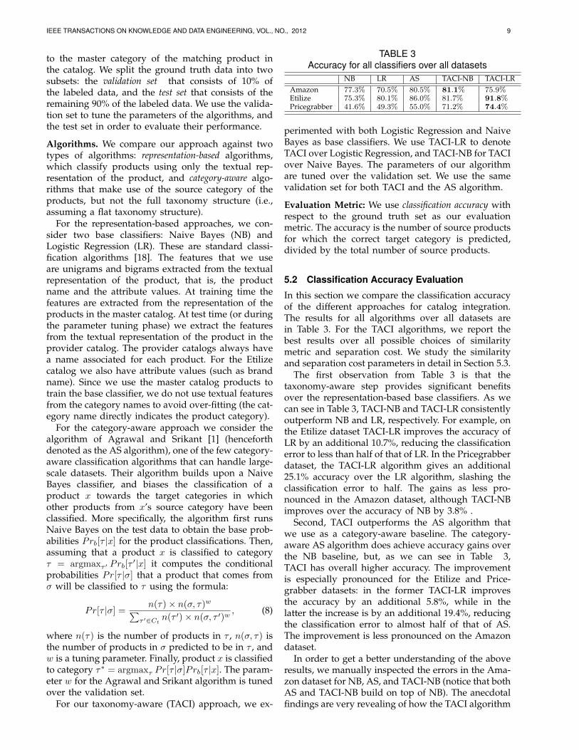
to the master category of the matching product inthe catalog. We split the ground truth data into twosubsets: the validation set that consists of 10% ofthe labeled data, and the test set that consists of theremaining 90% of the labeled data. We use the valida-tion set to tune the parameters of the algorithms, andthe test set in order to evaluate their performance.

Algorithms. We compare our approach against twotypes of algorithms: representation-based algorithms,which classify products using only the textual rep-resentation of the product, and category-aware algo-rithms that make use of the source category of theproducts, but not the full taxonomy structure (i.e.,assuming a flat taxonomy structure).

For the representation-based approaches, we con-sider two base classifiers: Naive Bayes (NB) andLogistic Regression (LR). These are standard classi-fication algorithms [18]. The features that we useare unigrams and bigrams extracted from the textualrepresentation of the product, that is, the productname and the attribute values. At training time thefeatures are extracted from the representation of theproducts in the master catalog. At test time (or duringthe parameter tuning phase) we extract the featuresfrom the textual representation of the product in theprovider catalog. The provider catalogs always havea name associated for each product. For the Etilizecatalog we also have attribute values (such as brandname). Since we use the master catalog products totrain the base classifier, we do not use textual featuresfrom the category names to avoid over-fitting (the cat-egory name directly indicates the product category).

For the category-aware approach we consider thealgorithm of Agrawal and Srikant [1] (henceforthdenoted as the AS algorithm), one of the few category-aware classification algorithms that can handle large-scale datasets. Their algorithm builds upon a NaiveBayes classifier, and biases the classification of aproduct x towards the target categories in whichother products from x’s source category have beenclassified. More specifically, the algorithm first runsNaive Bayes on the test data to obtain the base prob-abilities Prb[τ |x] for the product classifications. Then,assuming that a product x is classified to categoryτ = argmaxτ ′ Prb[τ

′|x] it computes the conditionalprobabilities Pr[τ |σ] that a product that comes fromσ will be classified to τ using the formula:

Pr[τ |σ] =n(τ)× n(σ, τ)w∑

τ ′∈Ct n(τ ′)× n(σ, τ ′)w, (8)

where n(τ) is the number of products in τ , n(σ, τ) isthe number of products in σ predicted to be in τ , andw is a tuning parameter. Finally, product x is classifiedto category τ∗ = argmaxτ Pr[τ |σ]Prb[τ |x]. The param-eter w for the Agrawal and Srikant algorithm is tunedover the validation set.

For our taxonomy-aware (TACI) approach, we ex-

TABLE 3Accuracy for all classifiers over all datasets

NB LR AS TACI-NB TACI-LRAmazon 77.3% 70.5% 80.5% 81.1% 75.9%Etilize 75.3% 80.1% 86.0% 81.7% 91.8%Pricegrabber 41.6% 49.3% 55.0% 71.2% 74.4%

perimented with both Logistic Regression and NaiveBayes as base classifiers. We use TACI-LR to denoteTACI over Logistic Regression, and TACI-NB for TACIover Naive Bayes. The parameters of our algorithmare tuned over the validation set. We use the samevalidation set for both TACI and the AS algorithm.

Evaluation Metric: We use classification accuracy withrespect to the ground truth set as our evaluationmetric. The accuracy is the number of source productsfor which the correct target category is predicted,divided by the total number of source products.

5.2 Classification Accuracy Evaluation

In this section we compare the classification accuracyof the different approaches for catalog integration.The results for all algorithms over all datasets arein Table 3. For the TACI algorithms, we report thebest results over all possible choices of similaritymetric and separation cost. We study the similarityand separation cost parameters in detail in Section 5.3.

The first observation from Table 3 is that thetaxonomy-aware step provides significant benefitsover the representation-based base classifiers. As wecan see in Table 3, TACI-NB and TACI-LR consistentlyoutperform NB and LR, respectively. For example, onthe Etilize dataset TACI-LR improves the accuracy ofLR by an additional 10.7%, reducing the classificationerror to less than half of that of LR. In the Pricegrabberdataset, the TACI-LR algorithm gives an additional25.1% accuracy over the LR algorithm, slashing theclassification error to half. The gains as less pro-nounced in the Amazon dataset, although TACI-NBimproves over the accuracy of NB by 3.8% .

Second, TACI outperforms the AS algorithm thatwe use as a category-aware baseline. The category-aware AS algorithm does achieve accuracy gains overthe NB baseline, but, as we can see in Table 3,TACI has overall higher accuracy. The improvementis especially pronounced for the Etilize and Price-grabber datasets: in the former TACI-LR improvesthe accuracy by an additional 5.8%, while in thelatter the increase is by an additional 19.4%, reducingthe classification error to almost half of that of AS.The improvement is less pronounced on the Amazondataset.

In order to get a better understanding of the aboveresults, we manually inspected the errors in the Ama-zon dataset for NB, AS, and TACI-NB (notice that bothAS and TACI-NB build on top of NB). The anecdotalfindings are very revealing of how the TACI algorithm


TABLE 4Classification accuracy for different similarity metrics

and separation costs.

Absolute MultiplicativeDifference Cost

PG

Shortest-Path 63.1% 62.7%

LCA 74.4% 62.1%

Cosine 69.7% 63.7%

Etil

ize Shortest-Path 91.3% 90.9%

LCA 91.7% 91.2%

Cosine 91.3% 90.6%

Am

azon Shortest-Path 77.2% 81.1%

LCA 80.6% 80.2%Cosine 79.6% 79.4%

manages to make use of the taxonomy structure.Consider the following example, which is actuallythe motivation example we used in the introduction.There are 272 products in the test set tagged with theAmazon category Electronics/Car Electronics/Car Audio &Video/Car Speakers/Coaxial Speakers which, accordingto the ground truth, map to the master categoryElectronics/Car Electronics/Car Audio/Car Speaker. How-ever, NB makes 138 errors, 118 of which correspondto products mapped to the category Electronics/HomeAudio/Speakers. This can be explained from the factthat the NB classifier has only access to the productrepresentation (i.e., the textual description), and therepresentation of a car speaker can be easily confusedwith the representation of a home audio speaker. TheAS algorithm makes fewer mistakes (68 in total), butTACI-NB is considerably better with just 21 errors.

The reason that the TACI-NB performs so well isthat there is a strong signal in the taxonomy thatthe algorithm is able to exploit. While at the leaflevel there is uncertainty about the right category,as we move upwards in the taxonomy tree it be-comes apparent that the car audio speakers shouldbe mapped to a subcategory of Car Electronics andnot Home Audio. For example, if we aggregate thepredictions of the NB classifier over all products inthe source category Electronics/Car Electronics/Car Audio& Video, 64% of them map to the target categoryElectronics/Car Electronics compared to 43% of the prod-ucts in Electronics/Car Electronics/Car Audio & Video/CarSpeakers/Coaxial Speakers that map to Electronics/CarElectronics/Car Audio/Car Speaker. It is precisely thishigher-level mappings between taxonomies that thetaxonomy-aware approach is able to take advantageof, while the category-aware approach is unable tomake use of this signal.

5.3 Similarity and Separation Cost Analysis

In this section we study the different similarity metricand separation cost options. Table 4 shows the accu-racy performance of the TACI algorithm for the threesimilarity measures we consider, and the two possibleseparation cost definitions, for all three datasets. The

taxonomy-aware step is applied on top of the best-performing baseline classifier. This is logistic regres-sion for Etilize and Pricegrabber, and the Naive Bayesfor Amazon. The accuracy numbers in bold are thebest for a specific similarity metric (best in the row),and the boxed numbers are the best for the specificdataset.

First, note that our technique demonstrates a consis-tent trend for all of the different choices of separationcost and similarity definitions. In the Etilize dataset,which appears to be amenable to the taxonomy-aware approach, all of the algorithms exhibit moreor less the same accuracy. In the Amazon dataset,where the taxonomy information appears to be min-imally helpful for the classification task, all of thealgorithms exhibit similar minimal gains (if any). Inthe PriceGrabber dataset, despite the variability in theresults, all of the algorithms exhibit gains of at least anadditional 10% with respect to the baseline classifieraccuracy.

Regarding the separation cost, Absolute Differenceoutperforms the Multiplicative Cost for most combi-nations of datasets and similarity metrics. A possibleexplanation for this is the symmetric property ofAbsolute Difference Cost. Because of this property,TACI helps eliminate base classifier mistakes thatclassify products from dissimilar categories in thesource taxonomy to close-by categories in the targettaxonomy.

Regarding the similarity metrics, the LCA similarityseems to perform the best overall. It has the highestaccuracy for Etilize and Pricegrabber, and it is closeto the best performance for Amazon. The LCA metriccaptures nicely the intuition that the similarity of twonodes in the taxonomy is determined by the point atwhich they merge (or split). It also fits well with theTACI approach that tries to make use of mappingsbetween ancestral nodes of two categories in orderto bias the classification. This intuition is not as wellcaptured by the Shortest-Path metric that does nottake into account the position of two nodes in thetaxonomy. The Cosine similarity is similar to LCA, butit penalizes differently two nodes depending on howdeep they are in the taxonomy. This is reasonable, butgiven that the parent relation in a taxonomy impliesalso subsumption (every SLR digital camera is also adigital camera), it is not always intuitive.

5.4 Running TimeIn this section we study the running time of ouralgorithm with respect to the number of products andthe number of categories in the source taxonomy. Weran our experiments on a Windows Server machinewith two 4-core Zeon E5504 processors at 2.0GHz. Weparallelized the algorithm for the preprocessing stepto make use of the full power of the 8 cores.

In our first experiment, we study the running timeof the taxonomy-aware calibration step as the num-


●

●

●

●

●

●

●

●

●

0 100 200 300 400 500

200

400

600

800

# products (x 1000)

time

(sec

)

(a) Preprocessing time (Pricegrabber)

●●

●●

●

●

●

●

●

0 100 200 300 400 500

510

1520

2530

35

# products (x 1000)

time

(sec

)

(b) Processing time (Pricegrabber)

Etilize Pricegrabber Amazon

product processingpreprocessing

010

030

050

070

0

(c) Running time (all datasets)

Fig. 2. Scalability experiments: Preprocessing and processing time for different samples of the Pricegrabberdataset. Comparison of total execution time for all three datasets.

ber of source catalog product increases using thePricegrabber dataset. In particular we subsampled 9different datasets from the Pricegrabber dataset ofsizes 10K, 25K, 50K, 75K, 100K, 200K, 300K, and 500K.Each sample is a subset of the immediately largersample We use the parameters γ, k and θ that weoptimized for the full Pricegrabber dataset.

Figures 2(a) and 2(b) show the preprocessing time(the loop in lines 12-13 of Algorithm 1), and theproduct processing time (the loop in lines 13-14)against the number of products in the dataset. Thefirst observation by looking at the y-axis scale for thetwo plots is that the running time is dominated bythat of the preprocessing step, which is an order ofmagnitude larger than that of the processing step.This is expected, since in the preprocessing step weperform essentially all of the computation necessaryfor classifying the open products in Oθ. Thus therunning time of the processing step is small, andscales in a linear way.

The running time of the preprocessing step dependson the number of candidate source-target categorypairs that we need to consider. As more products areintroduced, the number of candidate pairs increases.For very large datasets the number of candidate pairsshould saturate, and it should remain constant. Wedo observe a concave trend in our plot (the increasein the running time becomes smaller as the data sizegrows), but our dataset is not large enough for itto be clearly demonstrated. However, it is clear thatthe preprocessing time grows in a sublinear way,preserving our requirement for linear time processing.

In the second experiment we study the runningtime of the TACI algorithm as the number of sourcecatalog categories increases. We applied the TACI al-gorithm for all three datasets using the same number(50K) of products, so that we understand the effect ofthe spread of the products over different categories.The 50K Etilize products come from 201 categories,the 50K Pricegrabber products come from 653 differ-ent categories, and the 50K Amazon products comefrom 1,584 different categories. Figure 2(c) shows how

the preprocessing and processing running time variesfor the set of 50K products from the tree differentdatasets. The running time is again dominated by thepreprocessing time. Notice that in practice the runningtime increases almost linearly with the number ofcategories. This increase is significantly lower thanthe quadratic increase computed by the worst caseanalysis.

5.5 Parameter Sensitivity AnalysisThe tuning of the parameters is important to thecorrect operation of the TACI algorithm. We rely on avalidation set for this purpose. The validation set is asmall subset of the source catalog data for which wehave the true labeling in the target taxonomy. Sucha labeling is created through manual effort, or auto-mated techniques such as matching unique identifiers(e.g., UPC codes). Since the size of the validation setis typically small, this requires a manageable amountof effort. Still, there are cases where it may be hard toobtain such a validation set, or where the validationset is limited only to subsets of the catalog. In suchcases we can only obtain rough estimates of the bestpossible parameters.

In this section we study the sensitivity of the TACIalgorithm to the setting of the parameter values. Foreach of the three parameters k, γ, and θ, we considerseveral possible values and we will show that thereis a large range of parameter values for which weobtain results comparable to those obtained whenthe parameter values are set by the calibration step.For the parameter k that determines the number ofcandidate categories that we consider for an item, weconsider four different values K = {5, 10, 15, 20}. Forthe parameter γ that determines the tradeoff betweenthe assignment and separation cost, we consider sevendifferent possible values such that the ratio γ

1−γ takesvalues in the set Γ = {0.1, 0.2, 0.5, 1, 2, 5, 10}. Forthe parameter θ that determines the threshold onthe confidence of the base classifier, we consider tendifferent values. In order to deal with the variabilityof the output of the base classifier, and to be consistent


5 10 15 20

0.78

0.79

0.80

0.81

k

test

set

acc

urac

y

●

●●

●

●

TACI−optTACINB

(a) Parameter k

0.2 0.4 0.6 0.8 1.0

0.78

0.79

0.80

0.81

γ

test

set

acc

urac

y

●

●

●

●●

●

●

●

●

●

TACI−optTACINB

(b) Parameter γ

0.2 0.4 0.6 0.8

0.78

0.79

0.80

0.81

θ

test

set

acc

urac

y

●

●

●

●●

●

●

●

●●

TACI−optTACINB

(c) Parameter θ

Fig. 3. Sensitivity experiments on the Amazon dataset.

with the way we choose the values in the calibrationstep, we select the values for θ such we can control thefraction of the products for which we need to applythe taxonomy aware processing step. Since we haveten values for θ, this means that for the i-th value ofθ, 10i% of the products have probability less than thethreshold, and thus need to be processed.

In our experiment, for each dataset we considerthe version of the TACI algorithm that obtains thebest accuracy in Section 5.2. This is the TACI-LRfor Etilize and Pricegrabber, and the TACI-NB forAmazon. When testing the sensitivity of one of theparameters, we fix the other two to the values weused in the experiment in Section 5.2. We run theexperiment over the full labeled truth set, and wemeasure the accuracy of the specific parameter setting.In Figure 3 we present the results for the Amazondataset. The results of the other two datasets showedsimilar trends and they are omitted due to spaceconstraints. For each of the three parameters, weplot the accuracy we obtain for the values of theparameter we consider. In the plots the accuracy forthe different parameter values is denoted by TACI.For comparison’s sake we also plot the accuracy ofthe base classifier, and that of the TACI algorithm withthe parameters we obtained from the calibration step(denoted as “TACI-opt” in the plots).

Figure 3(a) shows that the algorithm does not seemaffected from the choice of the parameter k; we obtainmore or less the same accuracy for all values of k.Surprisingly, smaller k values seem to do better, andk = 5 outperforms the value k = 15 that we used inour experiments. However, the difference in accuracyis small.

As expected, the performance is more sensitive tothe setting of the tradeoff parameter γ that balancesthe weight between the assignment and the separationcosts. Figure 3(b) shows that for values of γ in therange between 0.5 and 0.75 the TACI accuracy is closeto the optimal. However, values of γ that are out ofthis range result in significantly worse accuracy, al-though it is still higher than the baseline NB accuracy.

The observations are similar for the setting of pa-

rameter θ. In Figure 3(c) we plot the accuracy versusthe fraction of products that are below the thresholdvalue of θ. When this fraction is between 0.2 and0.5, we obtain accuracy that is comparable that of thecalibrated TACI algorithm. For other values of θ theaccuracy drops significantly, but we still obtain someimprovement over the base classification.

In conclusion, the TACI algorithm is obviously af-fected from the setting of the parameters. However,when varying the parameters the accuracy plots aremostly smooth, and there is a range of values for allparameters for which the algorithm achieves perfor-mance comparable to that of the calibrated parametervalues. Thus, TACI is not overly sensitive to the exactsetting of the parameters, and it can perform compa-rably well for a wide range of parameter values.

6 RELATED WORK

Catalog Integration. To the best of our knowledge, noother scalable catalog integration approach exploitsthe structure of the product taxonomies. Previouswork makes use of source category information, buttreats the source and target taxonomies as flat. In theexperimental section, we compared our method withthe one of Agrawal and Srikant [1]. Their methodscales to large datasets (like ours), but it showedlower classification accuracy than our method in theexperiments. Sarawagi et al. introduce cross-training[28], which is an approach to semi-supervised learn-ing in the presence of multiple label sets. Unlikeour approach, they assume the existence of sometraining data labeled using both the source and mastertaxonomy. Their experimental results show that theaccuracy of cross-training in the catalog integrationproblem is comparable to the method of Agrawaland Srikant. Finally, Zhang et al. have also developedapproaches to catalog integration by using boosting[33] and transductive learning [32], [34]. Althoughthese approaches achieve better classification accuracythan AS, similar to the cross-training approach, theyrequire training data that are labeled in both thesource and the target taxonomies. So such methodsare not applicable to our problem setting.


Nandi and Bernstein [20] propose an approach formatching taxonomies based on query term distribu-tions. The approach is quite different to ours. First,it performs the mapping at the taxonomy level, map-ping categories from the source to the target, whilewe perform the mapping at the instance level bycategorizing individual product instances to the targettaxonomy. Secondly, the approach is not based onclassification but rather on exploiting distributions ofterms associated to the categories.

Metric Labeling and Structured Prediction. Ourformulation of the catalog integration problem asan optimization problem is inspired by the metriclabeling problem that was introduced in [12]. In themetric labeling problem, the goal is to find the optimallabeling of some objects so that they minimize anassignment and a separation cost. The problem isNP-hard [12] and the different existing approximatesolutions formulate it as an LP [12] or a QP [23]. Thecomplexity of these methods makes them inapplicableto large-scale datasets with more than a few hun-dreds of products. The objective of our optimizationproblem is also similar to the objective that arisesin computer vision problems [4], [5], [13]. The mostpopular application is image restoration, where thegoal is to restore the intensity of every pixel in animage using the values of the observed intensities. Thealgorithms developed in this area focus on separationcosts defined in the Euclidean space, i.e., the similarityof two items decreases linearly with their euclideandistance. Although such algorithms are scalable, theycannot be adapted to the separation cost definitionsthat are suitable for taxonomies.

Structured prediction—the study of machine learn-ing algorithms whose goal is to predict complexobjects with internal statistical dependencies—is anactive area of machine learning research [2]. It hasdirect applications to natural language processing,in which most prediction problems are structuredin nature: sequences of syntactic or semantic labelsfor words in a sentence (part of speech taggingor entity recognition), syntactic trees (parsing), for-eign language sentences (machine translation), graphmatchings (word- or sentence-alignment) or logicalforms (semantic parsing). In these areas, researchhas primarily focused either on the computationalproblem of test-time inference, which is typically adiscrete optimization problem [9], [14], [26], [27], [29],or of model training, which typically involves opti-mizing over an exponentially large set of potentialoutputs [7], [15], [25], [30]. Like these natural languageprocessing problems, our work involves recognizingstatistical dependencies in structured data; the pri-mary difference is that in our setting, the structuresare always known ahead of time and our goal is toleverage the information present in these structures.The most similar line of work in structured predictionto our setting is that of bipartite graph alignment

[10], [11], [19], which, in our application domain,would amount to trying to learn a generic taxonomyalignment model for arbitrary new portals making useof additional information in the taxonomies.

Ontology Alignment and Schema Matching. Thereis a large body of work in ontology alignment. Rep-resentative examples include Glue [8], a system thatuses machine learning to learn how to map betweenontologies; and Iliads [31], a system which makesuse of machine learning and logical inference tech-niques to output alignments. In general, the focusin ontology alignment is to map nodes of a sourcetaxonomy to nodes of a target taxonomy. In con-trast, in our work we are not interested in solvingthe (much harder) alignment problem between tax-onomies, but rather given an instance (i.e., a product)the goal is to categorize it in the target taxonomyusing aids from the taxonomy structure. The end-goal is always the categorization of the product.This distinction is very important in many practicalscenarios. For example, suppose that the source tax-onomy contains the leaf category Cameras, and thatit has no nodes that distinguish between differenttypes of cameras. Suppose that the target taxonomycontains the categories Cameras, Cameras/SLR DigitalCameras, and Cameras/Compact Cameras. An ontologyalignment technique would only be able to tell thatthe category Cameras in the source corresponds to thecategory Cameras in the target. However, given anactual product whose source category is Cameras, itis necessary to employ instance-level techniques likethe ones presented in this paper, to decide whether theproduct corresponds to Cameras/SLR Digital Cameras orCameras/Compact Cameras.

Similar considerations apply to schema matchingtechniques [22]. Such techniques find correspondencesbetween elements of different schemas, such as tablesand attributes. While the correspondences may beobtained by exploiting (aggregated) instance infor-mation, the output of schema matching techniquesis always given at the schema level. In our context,that represents associating categories of the mastertaxonomy to categories of the provider taxonomy. Incontrast, as we argued above, our techniques dealwith the different problem of determining for eachinput data instance element the appropriate categoryin the taxonomy. While schema matching techniquestypically exploit schema structure (e.g., a graph withedges based on foreign keys relations in similarityflooding [17]), the leveraged structure is significantlydifferent from the one that we exploit in this paper,namely hierarchical relationships in a taxonomy.

7 CONCLUSIONSIn this paper, we presented an efficient and scalableapproach to catalog integration that is based on theuse of source category and taxonomy structure infor-mation. We also showed that this approach leads to


substantial gains in accuracy with respect to existingclassifiers.

While we focused on shopping scenarios, our tech-niques are relevant to many other important domains.In particular, they are applicable to classification inany domain where there is a concept of a mastertaxonomy and there are information providers whichuse their own taxonomy to label the items that theyprovide. This includes important verticals such asLocal, Travel, Entertainment, etc. One example inEntertainment is the integration of media for stream-ing purposes. For instance, the Xbox Dashboard nowprovides the ability to access movies and TV showsfrom multiple providers, such as Netflix, Hulu, dif-ferent TV networks, etc. These providers use theirown taxonomy to label movies and shows, and thusthe need to properly organize them under a mastertaxonomy. As another example, in the Local domain,different providers may label restaurants in a differentway. For example, one provider may tag a restau-rant as “Ethnic/Greek” while another may tag it as“Mediterranean”.

While our techniques were used for classification,they can also be used for other problems. For example,their output could be be used as a feature for itemmatching, when we want to match elements classifiedunder the master taxonomy (e.g., the products in themaster catalog) to incoming offers from the providers.

For future work, we would like to explore semi-supervised learning techniques to incrementally re-train the base classifier with elements chosen duringthe taxonomy-aware calibration step. Finally, it wouldbe interesting to use our techniques in an active learn-ing setting, in order to identify candidate products forlabeling.

REFERENCES[1] R. Agrawal and R. Srikant. On integrating catalogs. In WWW,

pages 603–612, New York, NY, USA, 2001. ACM.[2] G. Bakir, T. Hofmann, B. Scholkopf, A. Smola, B. Taskar, and

S. Vishwanathan, editors. Predicting Structured Data. MITPress, 2007.

[3] G. Bakir, T. Hofmann, B. Schlkopf, A. Smola, B. Taskar, andS. Vishwanathan. Predicting Structured Data. MIT Press, 2007.

[4] Y. Boykov and V. Kolmogorov. An experimental comparisonof min-cut/max-flow algorithms for energy minimization invision. IEEE Transactions on Pattern Analysis and MachineIntelligence, 26(9):1124–1137, 2004.

[5] Y. Boykov, O. Veksler, and R. Zabih. Fast approximate energyminimization via graph cuts. IEEE Trans. Pattern Anal. Mach.Intell., 23(11):1222–1239, 2001.

[6] C. Chekuri, S. Khanna, J. S. Naor, and L. Zosin. Approx-imation algorithms for the metric labeling problem via anew linear programming formulation. In SODA, pages 109–118, Philadelphia, PA, USA, 2001. Society for Industrial andApplied Mathematics.

[7] H. Daume III, J. Langford, and D. Marcu. Search-basedstructured prediction. Machine Learning Journal, 2009.

[8] A. Doan, J. Madhavan, R. Dhamankar, P. Domingos, andA. Halevy. Learning to match ontologies on the semantic web.The VLDB Journal, 12(4):303–319, 2003.

[9] T. Finley and T. Joakims. Training structural SVMs when exactinference is intractable. In International Conference on MachineLearning (ICML), 2008.

[10] A. Fraser and D. Marcu. Getting the structure right for wordalignment: Leaf. In Empirical Methods in Natural Language Pro-cessing and Computational Natural Language Learning (EMNLP-CoNLL), 2007.

[11] J. Graca, K. Ganchev, and B. Taskar. Learning tractable wordalignment models with complex constraints. The ComputationalLinguistics Journal (CL), 36(3), 2010.

[12] J. Kleinberg and Eva Tardos. Approximation algorithmsfor classification problems with pairwise relationships: metriclabeling and markov random fields. J. ACM, 49(5):616–639,2002.

[13] V. Kolmogorov and R. Zabih. What energy functions can beminimizedvia graph cuts? IEEE Transactions on Pattern Analysisand Machine Intelligence, 26(2):147–159, 2004.

[14] A. Kulesza and F. Pereira. Structured learning with approxi-mate inference. In NIPS, 2007.

[15] P. Liang, H. Daume III, and D. Klein. Structure compilation:Trading structure for features. In International Conference onMachine Learning (ICML), 2008.

[16] T.-Y. Liu, Y. Yang, H. Wan, H.-J. Zeng, Z. Chen, and W.-Y. Ma.Support vector machines classification with a very large-scaletaxonomy. SIGKDD Explor. Newsl., 7(1):36–43, 2005.

[17] S. Melnik, H. Garcia-Molina, and E. Rahm. Similarity flooding:a versatile graph matching algorithm and its application toschema matching. In ICDE, pages 117–128, 2002.

[18] T. M. Mitchell. Machine Learning. McGraw-Hill, New York,1997.

[19] R. C. Moore, W. tau Yih, and A. Bode. Improved discriminativebilingual word alignment. In ACL, 2007.

[20] A. Nandi and P. A. Bernstein. Hamster: Using search clicklogsfor schema and taxonomy matching. PVLDB, 2(1):181–192,2009.

[21] C. Pesquita, D. Faria, A. O. Falco, P. Lord, and F. M. Couto.Semantic similarity in biomedical ontologies. PLoS ComputBiol, 5(7):e1000443, 07 2009.

[22] E. Rahm and P. Bernstein. A survey of approaches to automaticschema matching. The VLDB Journal, 10(4), 2001.

[23] P. Ravikumar and J. Lafferty. Quadratic programming re-laxations for metric labeling and markov random field mapestimation. In ICML, pages 737–744, New York, NY, USA,2006. ACM.

[24] P. Resnik. Using information content to evaluate semantic sim-ilarity in a taxonomy. In IJCAI, pages 448–453, San Francisco,CA, USA, 1995. Morgan Kaufmann Publishers Inc.

[25] S. Ross, G. J. Gordon, and J. A. Bagnell. A reduction of im-itation learning and structured prediction to no-regret onlinelearning. In AIStats, 2011.

[26] A. M. Rush and M. Collins. Exact decoding of syntactictranslation models through lagrangian relaxation. In ACL,2011.

[27] A. M. Rush, D. Sontag, M. Collins, and T. Jaakkola. On dualdecomposition and linear programming relaxations for naturallanguage processing. In EMNLP, 2010.

[28] S. Sarawagi, S. Chakrabarti, and S. Godbole. Cross-training:learning probabilistic mappings between topics. In KDD,pages 177–186, New York, NY, USA, 2003. ACM.

[29] V. Stoyanov, A. Ropson, and J. Eisner. Empirical risk min-imization of graphical model parameters given approximateinference, decoding, and model structure. In AISTATS, 2011.

[30] I. Tsochantaridis, T. Hofmann, T. Joachims, and Y. Altun. Largemargin methods for structured and interdependent outputvariables. JMLR, 6:1453–1484, Sep 2005.

[31] O. Udrea, L. Getoor, and R. J. Miller. Leveraging data andstructure in ontology integration. In SIGMOD, pages 449–460,New York, NY, USA, 2007. ACM.

[32] D. Zhang and W. S. Lee. Web taxonomy integration throughco-bootstrapping. In SIGIR, pages 410–417, New York, NY,USA, 2004. ACM.

[33] D. Zhang and W. S. Lee. Web taxonomy integration usingsupport vector machines. In WWW, pages 472–481, New York,NY, USA, 2004. ACM.

[34] D. Zhang, X. Wang, and Y. Dong. Web taxonomy integrationusing spectral graph transducer. In ER, pages 300–312, 2004.


Panagiotis Papadimitriou received thediploma degree in electrical and computerengineering from National Technical Univer-sity of Athens, Greece, in 2006, and the MSand PhD degrees in electrical engineeringfrom Stanford University, California, in 2008and 2011, respectively. He is currently a DataScientist at oDesk Research, Redwood City,California. His research interests include webadvertising, data privacy, labor marketplacesand web search. He is a recipient of an

Onassis Foundation scholarship for graduate studies and a Yahoo!Student Innovation Award.

Panayiotis Tsaparas is an Assistant Profes-sor at University of Ioannina, Greece. Beforethat he worked as a Researcher at MicrosoftResearch, and as a post-doctoral fellow atUniveristy of Helsinki, Finland and Univer-sity of Rome, La Sapienza. He received hisPh.D and M.Sc. degree from University ofToronto, and his B.Sc. degree from Univer-sity of Crete, Greece. His research interestsinclude Algorithmic Data Mining, Web Min-ing and Information Retrieval, Social Network

Analysis. He has served as a PC member for several data mining andweb conferences, such as KDD, WWW, and WSDM, and as AreaChair for ECML/PKDD.

Ariel Fuxman is a researcher at MicrosoftResearch Silicon Valley. His main researchareas are data mining, database manage-ment, and web search. He has served asPC member for conferences including SIG-MOD, VLDB, ICDE, CIKM, WWW, KDD. Hereceived his PhD. and MSc. from Universityof Toronto. He was awarded the SIGMODJim Gray Best Dissertation Award for hiswork on query answering over inconsistentdatabases.

Lise Getoor is an Associate Professor inthe Computer Science Department and theInstitute for Advanced Computer Studies atthe University of Maryland, College Park. Hermain research areas are machine learningand reasoning under uncertainty. She hasalso done work in areas such as databasemanagement, social network analysis andvisual analytics. She was the PC co-chair ofICML 2011, and has served as senior PC orPC member for conferences including AAAI,

ICML, IJCAI, ICWSM, KDD, SIGMOD, UAI, VLDB, and WWW. Shehas served as an ACM Transactions on Knowledge Discovery andData Associate Editor, a Journal of Artificial Intelligence ResearchAssociate Editor, and Machine Learning Journal Action Editor. Sheis on the board of the International Machine Learning Society, andhas served on the AAAI Council. She is a recipient of an NSFCareer Award, was a Microsoft New Faculty Fellow finalist and wasawarded a National Physical Sciences Consortium Fellowship. Shereceived her PhD from Stanford University, her Masters degree fromUniversity of California, Berkeley, and her BS from the University ofCalifornia, Santa Barbara.

IEEE TRANSACTIONS ON KNOWLEDGE AND DATA ENGINEERING, VOL., NO., 2012 I

APPENDIX ATHE SEPARATION COST

To define the separation cost we need to define thesimilarity and penalty functions. In this section wediscuss different possible definitions for both func-tions and outline their properties. We also discuss anormalization step that we apply to the separationcost function in our experiments, in order to alleviatethe effects of categories with large number of prod-ucts.

A.1 Category SimilarityCategory similarity in a taxonomy is a well-studiedtopic, and different metrics have been proposed. Catiaet al. [21] provide a good summary of such metrics.In this paper we present some representative metricsand we compare them in the experiments section.Recall that the value of simG(c1, c2) is the similarity ofcategories c1 and c2 in the taxonomy G. We considerthe following similarity measures.

Shortest-Path similarity: This similarity measure isdefined using the shortest path between two categoriesin the taxonomy tree. More specifically, the similaritybetween c1 and c2 is defined as follows:

simG(c1, c2) = 2−hops(c1,c2) (9)

where hops(c1, c2) is the length of the shortest pathbetween c1 and c2 in taxonomy G. We also applyan exponential decay function in order to furtherpenalize categories that are far apart. For example,if c1 = c2 then simG(c1, c2) = 1, if c1 is the parent ofc2 then simG(c1, c2) = 1/2, and if c1 and c2 have thesame parent then simG(c1, c2) = 1/4.

The shortest-path similarity has the property thatthe similarity is maximized when c1 = c2, which is adesirable property for a similarity function. However,since we use the similarity between categories todefine similarity between products, this has the effectthat two products under a high-level category such asElectronics are as similar as two products under a deep,specific category such as Electronics/Car Electronics/CarAudio/Car Speakers. Similarly, for two categories c1 andc2 that are children of the same node in the taxonomy,their similarity will always be simG(c1, c2) = 1/4, re-gardless of whether they are children of the root node,or of a node deep in the taxonomy. This stems fromthe fact that the similarity definition does not takeinto account the position of the categories within thetaxonomy tree, and the semantics of the subsumptionrelationship defined by the edges in a taxonomy.

LCA similarity: This similarity measure is definedusing the depth of the lowest common ancestorlca (c1, c2) of categories c1 and c2. More specifically,the similarity between c1 and c2 is defined as follows:

simG(c1, c2) = 1− 2−depth(lca(c1,c2)) (10)

The intuition for the use of the LCA comes fromthe work of Resnik [24]. Categories deeper in thetaxonomy, i.e., further away from the root node, aremore narrow and specific than categories higher in thetaxonomy, i.e., closer to the root. The LCA category ofc1 and c2 is the most specific category that subsumesboth categories. The deeper this category is, the higherthe similarity between c1 and c2.

For example, in the master taxonomy tree in Fig-ure 1 categories Electronics and Software have similar-ity 1/2, while categories Electronics/Car Electronics/CarAudio/Car Speakers and Electronics/Car Electronics/CarAudio/Car Amplifiers have similarity 7/8. Note that inthis definition if c1 = c2 = c then simG(c1, c2) =1− 2−depth(c). The similarity increases the deeper thecategory c, and it is not maximized. This makes sensein our scenario where we want products under a high-level category to be less similar than products undera deeper more specific category.

Cosine similarity: For this similarity measure, werepresent a category c using the categories in the pathfrom the root to category c. Let {x0, x1, ..., xd} denotethe set of categories in path from the root x0 =Root, tothe category xd = c, where d = depth (c) and xi ∈ Care categories in the taxonomy tree. We represent acategory c as a binary vector vc over the categoryspace C, that takes value 1 for each category x ∈ C inthe path from c to the root. Formally,

vc[x] =

{1 if category x ∈ {x0, x1, ..., xd};0 otherwise.

For example, the master taxonomy tree in Figure 1has 12 category nodes in total (including the root),and thus each category c is represented as a 12-dimensional binary vector. The vector for categoryElectronics takes value 1 for the entries of categoriesRoot and Electronics and zero for all other entries.The vector for category Electronics/Car Electronics/CarAudio takes values 1 for the entries of categories Root,Electronics, Electronics/Car Electronics and Electronics/CarElectronics/Car Audio.

Given the vector representation we can now definethe similarity of two categories c1 and c2 as the cosinesimilarity of their corresponding vectors v1 and v2.The cosine of the two vectors is defined as

cos(v1, v2) =v1 · v2

|v1||v2|

Where v1 · v2 is the dot product of the two vectorsand |v| is the length of the vector v. Note that thenumber of 1’s in a category vector vc is equal to thenumber of categories in the path of category c tothe root, which is equal to 1 + depth (c). Therefore,|vc| =

√1 + depth (c). The dot product of two binary

vectors is equal to the number of entries for whichboth vectors have value 1. Since the vectors representpaths in the tree, this is the number of categories in

IEEE TRANSACTIONS ON KNOWLEDGE AND DATA ENGINEERING, VOL., NO., 2012 II

the path from the least common ancestor to the root.That is, v1 · v2 = 1 + depth (lca (c1, c2)).

Therefore, we can compute the cosine similaritybetween categories c1 and c2 as follows:

simG(c1, c2) =1 + depth (lca (c1, c2))√

1 + depth (c1)√

1 + depth (c2)(11)

Using this similarity measure, two categories c1 andc2 are similar if their lowest common ancestor is deepin the taxonomy, and categories c1 and c2 are closeto their least common ancestor, that is their shortestpath is small. For example, in the master taxonomytree in Figure 1 categories Electronics/Car Electronicsand Electronics/Home Audio are more similar than Elec-tronics/Car Electronics/Car Audio and Electronics/Home Au-dio/Speakers since the former pair is closer to theirleast common ancestor Electronics. The measure hasalso the property that similarity of a category to itselfis 1. Furthermore, categories that are deeper in thetaxonomy are more similar than categories that arehigher in taxonomy.

Given the set representation of a category c, wecan also use other set similarity measures such as theDice and Jaccard coefficient. We experimented withthese similarity measures, and we obtained resultsvery similar with the cosine similarity, so we do notreport them in this paper.

We note that our problem formulation is not tied toany specific similarity measure; any similarity mea-sure can be utilized. We compare experimentally themeasures we defined in this section in Section 5.3where we also discuss how their properties affect theirperformance.

A.2 The Penalty Function

To complete the definition of the separation cost, weneed to define the penalty function δ that we willuse. In this paper we consider the following twodefinitions for the penalty function, and, as a result,two different definitions for the the separation cost.

Absolute Difference Cost: The penalty function is theabsolute difference between the similarities in the twotaxonomies:

SCOST(sx, sy, `x, `y) = |simS(sx, sy)− simT (`x, `y)|(12)

The absolute difference cost is symmetric: it penalizesboth the placement of similar products in dissimilarcategories, and the placement of dissimilar productsin similar categories.

We also experimented with the squared differencebetween the similarities as a candidate penalty func-tion. We observed similar results, and we do notreport them in this paper.

Multiplicative Cost: The penalty function is the dis-similarity (1− simT (`x, `y)) of the categories `x and `y

in the target taxonomy T , weighted by the similaritysimS(sx, sy) of sx and sy in the source taxonomy S:

SCOST(sx, sy, `x, `y) = simS(sx, sy)(1− simT (`x, `y))(13)

This definition is inspired by the metric labelingproblem [12] and yields an asymmetric cost. That is,the cost penalizes similar products (high simS(sx, sy))that are classified to dissimilar target categories (lowsimT (`x, `y)), but it does not penalize heavily dissimi-lar products that are placed in similar categories. Sucha property is useful if the target taxonomy containscombined categories that correspond to different cate-gories in the source taxonomy, e.g., target has categoryComputing & Electronics while the source taxonomy hastwo separate categories Computing and Electronics.

We discuss the differences between the two penaltyfunctions along with their performance comparison inSection 5.3 of the experiments.

A.3 NormalizationIn our experiments we normalize the separationcost SCOST(sx, sy, `x, `y) by a normalization parameterρ(sx, sy). The reason for the normalization is that inpractice we observed that the distribution of productsinto the source taxonomy may have a significantimpact on the results. Categories that have a verylarge number of products can pull in products fromdistant categories, simply because of their size. This iscommon in large web taxonomies, where the distribu-tion of the number of objects per category is often veryskewed (e.g., power-law or log-normal [16]). In thesecases, separating the products from small-size sourcecategories from the products of a large source categoryincurs a high penalty, and thus our optimizationtechnique will tend to merge products from small cat-egories together with those of the large category in thetarget taxonomy. The normalization parameter servesthe purpose of eliminating this “gravitational pull” ofcategories with very large number of products.

We calculate the normalization factor ρ as follows.Let x and y be two products, and sx and sy be theirrespective source categories. We compute ρ(sx, sy) asthe total number of products whose source categoryis at the same similarity radius from sx as sy :

ρ(sx, sy) =∑σ:simG(sx,σ)=simG(sx,sy) n(σ) (14)

where n(σ) is the total number of products in sourcecategory σ. Note that the normalization factor it isasymmetric, that is, it is a normalization with respectto x instead of being symmetric with respect to thepair x, y. It is easy to make it symmetric by taking thesum or average. However, we define it asymmetric onpurpose, since in Section 4 we compute the separationof an element x with respect to a set of already clas-sified elements. This normalization factor was shownto perform well in our experiments, prohibiting largecategories from attracting too many products.

TACI: Taxonomy-Aware Catalog Integration - Stanford University

Documents

Transcript of TACI: Taxonomy-Aware Catalog Integration - Stanford University