^ecknical v2©te 191

Tables Describing Small-Sample Properties of the

Mean, Median, Standard Deviation, and Other Statistics

In Sampling From Various Distributions

CHURCHILL EISENHART, LOLA S. DEMING

AND CELIA S. MARTIN

U. S. DEPARTMENT OF COMMERCENATIONAL BUREAU OF STANDARDS

THE NATIONAL BUREAU OF STANDARDS

Functions and Activities

The functions of the National Bureau of Standards arc set forth in the Act of Congress,

March 3, 1901, as amended by Congress in Public Law 619, 1950. These include the develop-

ment and maintenance of the national standards of measurement and the provision of meansand methods for making measurements consistent with these standards; the determination of

physical constants and properties of materials; the development of methods and instruments

for testing materials, devices, and structures; advisory services to government agencies onscientific and technical problems; invention and development of devices to serve special needs

of the Government; and the development of standard practices, codes, and specifications. Thework includes basic and applied research, development, engineering, instrumentation, testing,

evaluation, calibration services, and various consultation and information services. Research

projects are also performed for other government agencies when the work relates to and supple-

ments the basic program of the Bureau or when the Bureau's unique competence is required.

The scope of activities is suggested by the listing of divisions and sections on the inside of

the back cover.

Publications

The results of the Bureau's research are published cither in the Bureau's own series of

publications or in the journals of professional and scientific societies. The Bureau publishes

three periodicals available from the Government Printing Office: The Journal of Research,

published in four separate sections, presents complete scientific and technical papers; the. Tech-

nical News Bulletin presents summary and preliminary reports on work in progress; and the

Central Radio Propagation Laboratory Ionospheric Predictions provides data for determining

the best frequencies to use for radio communications throughout the world. There are also

five series of nonperiodical publications: Monographs, Applied Mathematics Series, Handbooks,Miscellaneous Publications, and Technical Notes.

A complete listing of the Bureau's publications can be found in National Bureau of Stand-

ards Circular 400, Publications of the National Bureau of Standards, 1901 to June 1947 ($1.25),

and the Supplement to National Bureau of Standards Circular 460, July 1947 to June 1957

($1.50), and Miscellaneous Publication 240, July 1957 to June 1960 (includes Titles of Papers

Published in Outside Journals 1950 to 1959) ($2.25): available from the Superintendent of

Documents, Government Printihg Office, Washington 25, D.C.

NATIONAL BUREAU OF STANDARDS

TecAmcaf ^ote 191

ISSUED JUNE 14, 1963

Tables Describing Small-Sample Properties of the

Mean, Median, Standard Deviation, and Other Statistics

In Sampling From Various Distributions

Churchill Eisenhart, Lola S. Deming

and Celia S. Martin

NBS Technical Notes are designed to supplement the Bu-reau's regular publications program. They provide a

means for making available scientific data that are of

transient or limited interest. Technical Notes may belisted or referred to in the open literature.

For sale by the Superintendent of Documents, U.S. Government Printing Office

Washington 25, D.C. Price 20 cents

FOREWORD

As part of a continuing program of research into statistical methods

appropriate for measurement and calibration programs in the physical sciences

and engineering, the Statistical Engineering Laboratory of the National

Bureau of Standards conducts studies of the properties that would be exhibited

by frequently-used statistical techniques if they v.'ere applied to data obey-

ing a variety of probability distributions. This note makes generally

available the tables that were described in three related papers, presented

before a joint session of the American Mathematical Society and the Institute

of Mathematical Statistics in Madison, Wisconsin, on September 7, 1948.

Copies of these tables were distributed to persons present at this session;

and copies of some of them have been made available to various other persons

from time to time during the intervening years. These tables were not

submitted for formal publication heretofore because each represented unfin-

ished portions of a larger study that subsequently evolved in a manner

different from that originally contemplated. The tables are published now,

for convenient reference, accompanied by the (slightly edited) brief

descriptions of them that appeared as Abstracts in the Annals of Mathematical

Statistics , Vol. 19, pp. 598-600 (1948). During the intervening years more

accurate values have become available for the standard deviation of the

median in small samples from the normal and double-exponential distributions;

the final columns of Tables lb and 2b were revised accordingly.

March 1963 Churchill Eisenhart, ChiefStatistical Engineering

Laboratory

ii

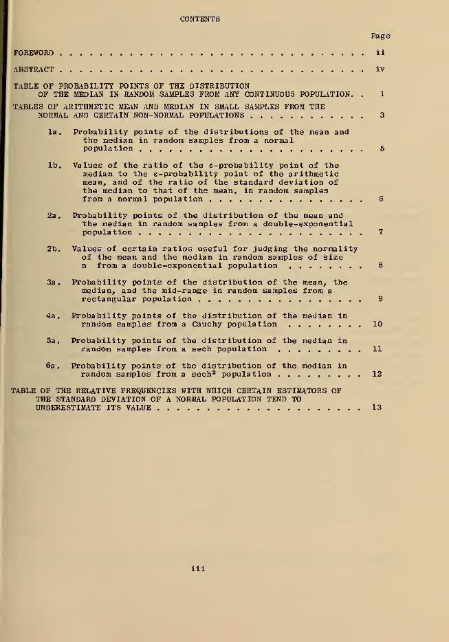
CONTENTS

Page

FOREWORD ii

ABSTRACT iv

TABLE OF PROBABILITY POINTS OF THE DISTRIBUTIONOF THE MEDIAN IN RANDOM SAMPLES FROM ANY CONTINUOUS POPULATION. . 1

TABLES OF ARITHMETIC MEAN AND MEDIAN IN SMALL SAMPLES FROM THENORMAL AND CERTAIN NON-NORMAL POPULATIONS 3

la. Probability points of the distributions of the mean andthe median in random samples from a normalpopulation 5

lb. Values of the ratio of the e-probability point of themedian to the e-probability point of the arithmeticmean, and of the ratio of the standard deviation ofthe median to that of the mean, in random samplesfrom a normal population 6

2a. Probability points of the distribution of the mean andthe median in random samples from a double-exponentialpopulation 7

2b. Values of certain ratios useful for judging the normalityof the mean and the median in random samples of sizen from a double-exponential population 8

3a. Probability points of the distribution of the mean, themedian, and the mid-range in random samples from arectangular population 9

4a. Probability points of the distribution of the median inrandom samples from a Cauchy population 10

5a. Probability points of the distribution of the median inrandom samples from a sech population 11

6a. Probability points of the distribution of the median inrandom samples from a sech2 population 12

TABLE OF THE RELATIVE FREQUENCIES WITH WHICH CERTAIN ESTIMATORS OFTHE STANDARD DEVIATION OF A NORMAL POPULATION TEND TOUNDERESTIMATE ITS VALUE 13

iii

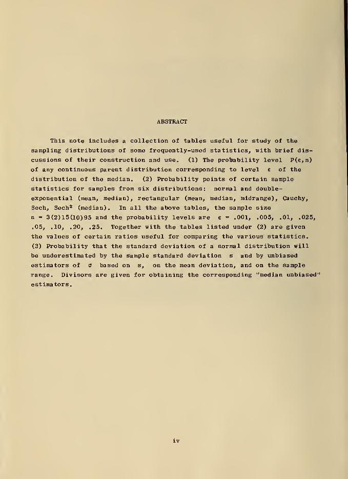
ABSTRACT

This note includes a collection of tables useful for study of the

sampling distributions of some frequently-used statistics, with brief dis-

cussions of their construction and use. (1) The probability level P(e,n)

of any continuous parent distribution corresponding to level e of the

distribution of the median. (2) Probability points of certain sample

statistics for samples from six distributions: normal and double-

exponential (mean, median), rectangular (mean, median, midrange), Cauchy,

Sech, Sech2 (median). In all the above tables, the sample size

n - 3(2)15(10)95 and the probability levels are e - .001, .005, .01, .025,

.05, .10, .20, .25. Together with the tables listed under (2) are given

the values of certain ratios useful for comparing the various statistics.

(3) Probability that the standard deviation of a normal distribution will

be underestimated by the sample standard deviation s and by unbiased

estimators of a based on s, on the mean deviation, and on the sample

range. Divisors are given for obtaining the corresponding "median unbiased"

estimators.

iv

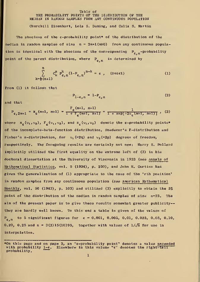
Table ofTHE PROBABILITY POINTS OF THE DISTRIBUTION OF THE

MEDIAN IN RANDOM SAMPLES FROM ANY CONTINUOUS POPULATION

Churchill Eisenhart, Lola S. Deming, and Celia S. Martin

The abscissa of the e-probability point* of the distribution of the

median in random samples of size n = 2m+l(ma0) from any continuous popula-

tion is identical with the abscissa of the corresponding P -probability

point of the parent distribution, where P is determined bySt u

n

I Cl Pe,n

(1 -Pe ,n>

n_k= e

* <°*eSl > ">k=|(n+l)

From (1) it follows that

P, = 1-P (2)l-e,n e,n

and that

F (m+1, m+1) ,s 1

'e^m+l " xc(ra+1

'ra+1) " 1 + F (m+1, m+1) ~ 1 + expl-2z (m+1, m+1)

J'

(3)

where x_(v 1 ,v 2 )> F (v x ,v 2 ), and z (v t ,v 2 ) denote the e-probability points*

of the incomplete-beta-function distribution, Snedecor's F-distribution and

Fisher's z-distribution, for v t (=»2q) and v 2 (=2p) degrees of freedom,

respectively. The foregoing results are certainly not new: Harry S. Pollard

implicitly utilized the first equality on the extreme left of (3) in his

doctoral dissertation at the University of Wisconsin in 1933 (see Annals of

Mathematical Statistics , vol. 5 (1934), p. 250), and John H. Curtiss has

given the generalization of (1) appropriate to the case of the 'rth position'

in random samples from any continuous population (see American Mathematical

Monthly , vol. 50 (1943), p. 103) and utilized (3) explicitly to obtain the 5%

point of the distribution of the median in random samples of size n-23. The

aim of the present paper is to give these results somewhat greater publicity

—

they are hardly well known. To this end a table is given of the values of

P to 5 significant figures for e - 0.001, 0.005, 0.01, 0.025, 0.05, 0.10,

0.20, 0.25 and n - 3(2)15(10)95, together with values of 1/Vn for use in

interpolation.

*0n this page and on page 2, an "e-probability point" denotes a value exceededwith probability 1-e . Elsewhere in this volume "e'' denotes the right-tailprobability.

1

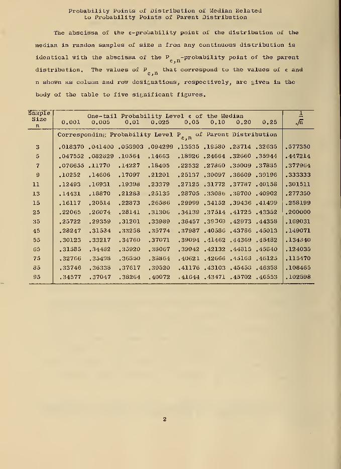
Probability Points of Distribution of Median Relatedto Probability Points of Parent Distribution

The abscissa of the e-probability point of the distribution of the

median in random samples of size n from any continuous distribution is

identical with the abscissa of the P -probability point of the parent

distribution. The values of P that correspond to the values of e ande,n

n shown as column and row designations, respectively, are given in the

body of the table to five significant figures.

SampleSizen

One-tail Probab ility Level e of the Median 1

0.001 0.005 0.01 0.025 0.05 0.10 0.20 0.25 JS

Corresponding Probabili ty Level P ofe,n

Parent Distra bution

3 .013370 .041400 .053903 .094299 .13535 .19580 .23714 .32635 .577350

5 .047552 .082829 .10564 .14663 .18926 .24664 .32660 .35944 .447214

7 .076655 .11770 .14227 .18405 .22532 .27860 .35009 .37885 .377964

9 .10252 .14606 .17097 .21201 .25137 .30097 .36609 .39196 .333333

11 .12493 .16931 .19398 .23379 .27125 .31772 .37787 .40158 .301511

13 .14431 .18870 .21283 .25135 .28705 .33086 .38700 .40902 .277350

15 .16117 .20514 .22873 .26586 .29999 .34152 .39436 .41499 .258199

25 .22065 .26074 .28141 .31306 .34139 .37514 .41725 .43352 .200000

35 .25722 .29359 .31201 .33989 .36457 .39369 .42973 .4435S .169031

45 .28247 .31534 .33258 .35774 .37987 .40586 .43786 .45013 .149071

55 .30123 .33217 .34760 .37071 .39094 .41462 .44369 .45482 .134340

65 .31585 .34482 .35920 .38067 .39942 .42132 .44815 .45840 .124035

75 .32766 .35498 .36850 .33864 .40621 .42666 .45163 .46125 .115470

85 .33746 .36338 .37617 .39520 .41176 .43103 .45458 .46358 .108465

95 .34577 .37047 .38264 .40072 .41644 .43471 .45702 .46553 .102598

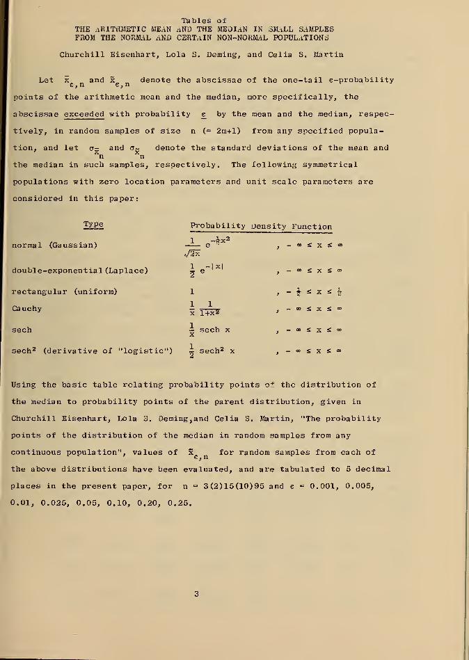
Tables ofTHE ARITHMETIC MEAN AND THE MEDIAN IN SMALL SAMPLESFROM THE NORMAL AND CERTAIN NON-NORMAL POPULATIONS

Churchill Eisenhart, Lola S. Deming, and Celia S. Martin

Let x and x denote the abscissae of the one-tail e-probabilitye, n e, n r j

points of the arithmetic mean and the median, more specifically, the

abscissae exceeded with probability £ by the mean and the median, respec-

tively, in random samples of size n (= 2m+l) from any specified popula-

tion, and let <j- and a~ denote the standard deviations of the mean andx xn n

the median in such samples, respectively. The following symmetrical

populations with zero location parameters and unit scale parameters are

considered in this paper:

.A-w-2

„/2x

e "•

Type

normal (Gaussian)

double-exponential (Laplace)

rectangular (uniform)

Cauchy

sech

sech 2 (derivative of ''logistic") ~ sech2 x

Probability Density Function

12" e-

|X

1

1 1

x 1+X2

1

Xsech X

- oo £ X £ "°

- oo £ x £ oo

- i * X £ *

- oo S x S oo

oo £ X S o°

- oo S x £ «

Using the basic table relating probability points of the distribution of

the median to probability points of the parent distribution, given in

Churchill Eisenhart, Lola 3. Deming^and Celia S. Martin, "The probability

points of the distribution of the median in random samples from any

continuous population", values of x for random samples from each of

the above distributions have been evaluated, and are tabulated to 5 decimal

places in the present paper, for n = 3(2)15(10)95 and e = 0.001, 0.005,

0.01, 0.025, 0.05, 0.10, 0.20, 0.25.

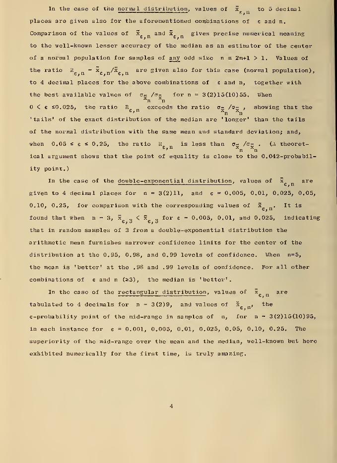
In the case of the normal distribution , values of x to 5 decimal

places are given also for the aforementioned combinations of e and n.

Comparison of the values of x and x gives precise numerical meaninge, n e, n ° a

to the well-known lesser accuracy of the median as an estimator of the center

of a normal population for samples of any odd size n =. 2m+l > 1. Values of

the ratio R = x _/x are given also for this case (normal population),

to 4 decimal places for the above combinations of e and n, together with

the best available values of a~ /a- for n = 3(2)15(10)55. Whenxn n

< e £0.025, the ratio R exceeds the ratio o~ /a- , showing that the' n n

'tails' of the exact distribution of the median are 'longer' than the tails

of the normal distribution with the same mean and standard deviation; and,

when 0.05 « e < 0.25, the ratio R is less than o~ /a- . (A theoret-' e,

n

xx' n n

ical argument shows that the point of equality is close to the 0.042-probabil-

ity point.)

In the case of the double-exponent ia l distribution , values of x are

given to 4 decimal places for n = 3(2)11, and e = 0.005, 0.01, 0.025, 0.05,

0.10, 0.25, for comparison with the corresponding values of x .It is

found that when n = 3, x „<x _ for e = 0.005, 0.01, and 0.025, indicating

that in random samples of 3 from a double-exponential distribution the

arithmetic mean furnishes narrower confidence limits for the center of the

distribution at the 0.95, 0.98, and 0.99 levels of confidence. When n=5,

the mean is 'better' at the .98 and .99 levels of confidence. For all other

combinations of e and n (s3), the median is 'better'.

In the case of the rectangular distribution, values of x are

tabulated to 4 decimals for n = 3(2)9, and values of x , the

e-probability point of the mid-range in samples of n, for n = 3(2)15(10)95,

in each instance for e = 0.001, 0.005, 0.01, 0.025, 0.05, 0.10, 0.25. The

superiority of the mid-range over the mean and the median, well-known but here

exhibited numerically for the first time, is truly amazing.

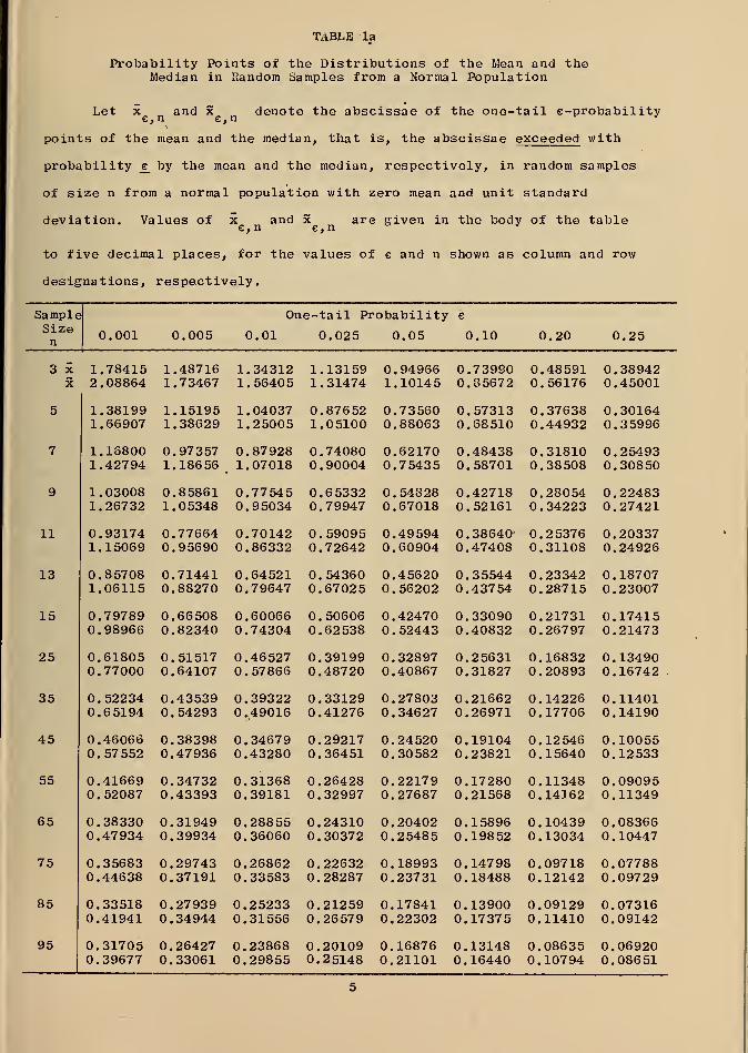
TABLE la

Probability Points of the Distributions of the Mean and theMedian in Random Samples from a Normal Population

Let x and x denote the abscissae of the one-tail s-probabilitye, n e,n

points of the mean and the median, that is, the abscissae exceeded with

probability e_ by the mean and the median, respectively, in random samples

of size n from a normal population with zero mean and unit standard

deviation. Values of x and x are given in the body of the tablee, n e,n

to five decimal places, for the values of e and n shown as column and row

designations, respectively.

Sample One-tail Probability e

Sizen

0.001 0.005 0.01 0.025 0.05 0.10 0.20 0.25

3 xX

1.784152.08864

1.487161.73467

1.343121.56405

1.131591.31474

0.949661.10145

0.739900.85672

0.485910.56176

0.389420.45001

5 1.381991 . 66907

1.151951.38629

1.040371.25005

0.876521.05100

0.735600.88063

0.573130.68510

0.376380.44932

0.301640.35996

7 1.158001.42794

0.973571.18656

0.879281.07018

0.74080. 90004

0.621700.75435

0.484380.58701

0.318100.38508

0.254930.30850

9 1.030081.26732

0.858611.05348

0.775450.95034

0.653320.79947

0.548280.67018

0.427180.52161

0.280540.34223

0.224830.27421

11 0.931741.15069

0.776640.95690

0.701420.86332

0.590950.72642

0.495940.60904

0.38640-0.47408

0.253760.31108

0.203370.24926

13 0.857081.06115

0.714410.88270

0.645210.79647

0.543600.67025

0.456200.56202

0.355440.43754

0.233420.28715

0.187070.23007

15 0.797890.98966

0.665080.82340

0.600660.74304

0.506060.62538

0.424700.52443

0.330900.40832

0.217310.26797

0.174150.21473

25 0.618050.77000

0.515170.64107

0.465270.57866

0.391990.48720

0.328970.40867

0.256310.31827

0.168320.20893

0.134900.16742 .

35 0.522340.65194

0.435390.54293

0.393220^49016

0.331290.41276

0.278030.34627

0.216620.26971

0.142260.17706

0.114010.14190

45 0.460660.57 552

0.383980.47936

0.346790.43280

0.292170.36451

0.245200.30582

0.191040.23821

0.125460.15640

0.100550.12533

55 0.416690.52087

0.347320.43393

0.313680.39181

0.264280.32997

0.221790.27687

0.172800.21568

0.113480.14162

0.090950.11349

65 0.383300.47934

0.319490.39934

0.288550.36060

0.243100.30372

0.204020.25485

0.158960.19852

0.104390.13034

0.083660.10447

75 0.356830.44638

0.297430.37191

0.268620.33583

0.226320.28287

0.189930.23731

0.147980.18488

0.097180.12142

0.077880.09729

85 0.335180.41941

0.279390.34944

0.252330.31556

0.212590.26579

0.178410.22302

0.139000.17375

0.091290.11410

0.073160.09142

95 0.317050.39677

0.264270.33061

0.238680.29855

0.201090.25148

0.168760.21101

0.131480.16440

0.086350.10794

0.069200.08651

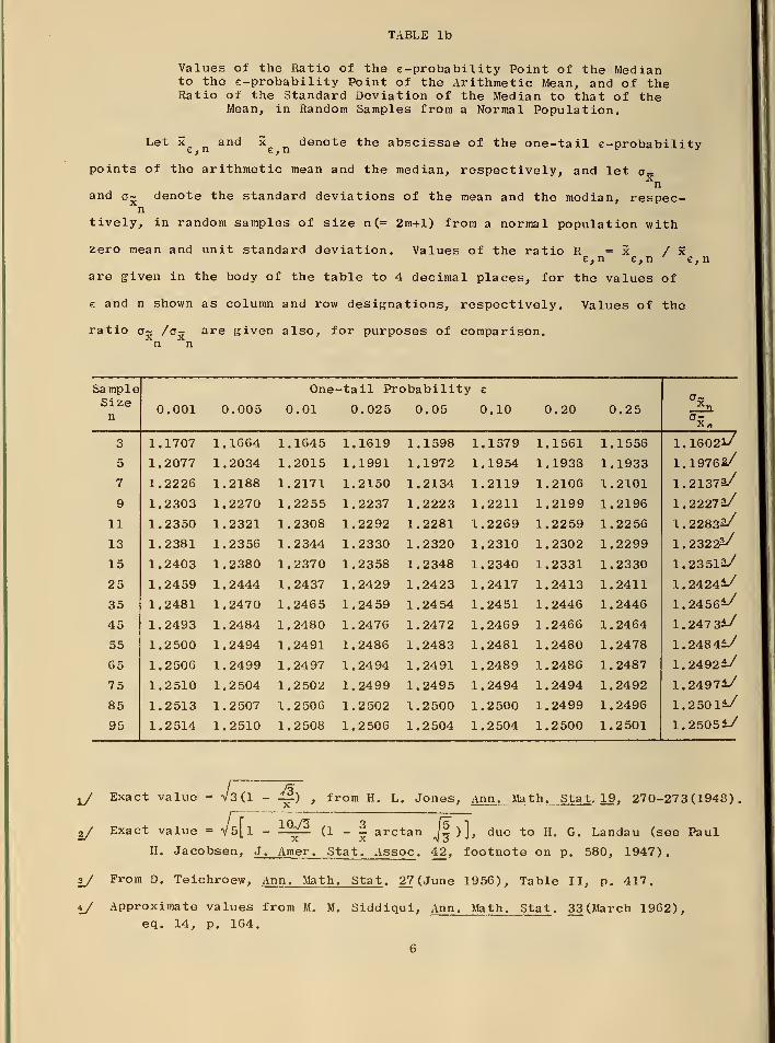
TABLE lb

Values of the Ratio of the e-probability Point of the Medianto the e-probability Point of the Arithmetic Mean, and of theRatio of the Standard Deviation of the Median to that of the

Mean, in Random Samples from a Normal Population.

Let x and x denote the abscissae of the one-tail e-probability

points of the arithmetic mean and the median, respectively, and let a-xnand o~ denote the standard deviations of the mean and the median, respec-

ntively, in random samples of size n (= 2m+l) from a normal population with

zero mean and unit standard deviation. Values of the ratio R = x / xe,n e, n e, n

are given in the body of the table to 4 decimal places, for the values of

e and n shown as column and row designations, respectively. Values of the

ratio a~ /a- are given also, for purposes of comparison,n n

SampleSizen

0.001 0.005

One

0.01

-tail Probability e

0.025 0.05 0.10 0.20 0.25ax„

3 1.1707 1.1664 1.1645 1.1619 1.1598 1.1579 1.1561 1.1556 1.1602l/

5 1.2077 1.2034 1.2015 1.1991 1.1972 1.1954 1.1933 1.1933 1.19762/

7 1.2226 1.2188 1.2171 1.2150 1.2134 1.2119 1.2106 1.2101 1.21372/

9 1.2303 1.2270 1.2255 1.2237 1.2223 1.2211 1.2199 1.2196 1.22272/

11 1.2350 1.2321 1.2308 1.2292 1.2281 1.2269 1.2259 1.2256 1.22832/

13 1.2381 1.2356 1.2344 1.2330 1.2320 1.2310 1.2302 1.2299 1.23222/

15 1.2403 1.2380 1.2370 1.2358 1.2348 1.2340 1.2331 1.2330 1.23512/

25 1.2459 1 . 2444 1.2437 1.2429 1.2423 1.2417 1.2413 1.2411 1.2424*/

35 1.2481 1.2470 1.2465 1.2459 1.2454 1.2451 1.2446 1.2446 1.2456*-/

45 1.2493 1.2484 1.2480 1.2476 1.2472 1.2469 1.2466 1.2464 1.247 3*/

55 1.2500 1.2494 1.2491 1.2486 1.2483 1.2481 1.2480 1.2478 1.248 4*/

65 1.2506 1.2499 1.2497 1.2494 1.2491 1.2489 1.2486 1.2487 1.2492*/

75 1.2510 1.2504 1.2502 1.2499 1.2495 1.2494 1.2494 1.2492 1.2497*/

85 1.2513 1.2507 1.2506 1.2502 1.2500 1.2500 1.2499 1.2496 1.2501*/

95 1.2514 1.2510 1.2508 1.2506 1.2504 1.2504 1.2500 1.2501 1.2505*/

J* V3\jj Exact value = V3(l - ~) , from H. L. Jones, Ann. Math. Stat . 19. 270-273(1948).

2/ Exact value = V5[l - ~^£ (1 - | arctan J|)], due to H. G. Landau (see Paul

H. Jacobsen, J. Amer. Stat. Assoc . 42, footnote on p. 580, 1947).

3/ From D. Teichroew, Ann. Math. Stat . 27 (June 1956), Table II, p. 417.

4/ Approximate values from M. M. Siddiqui, Ann. Math. Stat . 33(March 1962),eq. 14, p. 164.

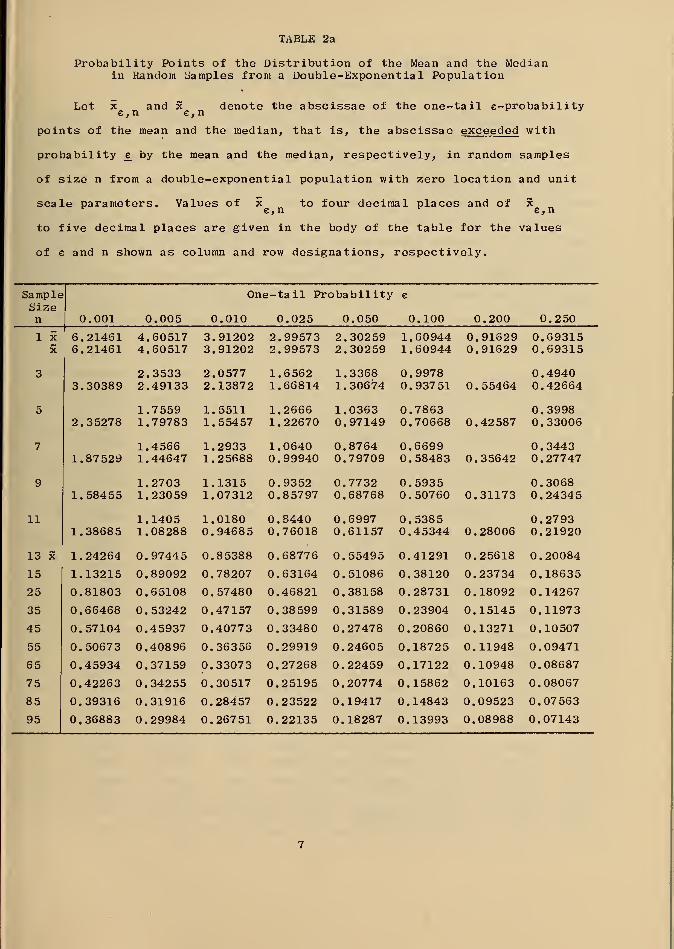
TABLE 2a

Probability Points of the Distribution of the Mean and the Medianin Random Samples from a Double-Exponential Population

Let x and x denote the abscissae of the one-tail e-probabilitye, n e,

n

points of the mean and the median, that is, the abscissae exceeded with

probability e^ by the mean and the median, respectively, in random samples

of size n from a double-exponential population with zero location and unit

scale parameters. Values of x to four decimal places and of xe,

n

r e,

n

to five decimal places are given in the body of the table for the values

of e and n shown as co lumn and row designations, respectively.

SampleSizen 0.001 0.005

One-tail Probability

0.010 0.025 0.050

G

0.100 0.200 0.250

1 XX

3

6.214316.21461

3.30389

4.605174.60517

2.35332.49133

3.912023.91202

2.05772.13872

2.995732.99573

1.65621.66814

2.302592.30259

1.33681.30674

1.609441.60944

0.99780.93751

0.916290.91629

0.55464

0.693150.69315

0.49400.42664

7

9

11

2.35278

1.87529

1.58455

1.75591.79783

1.45661.44647

1.27031.23059

1.55111.55457

1.29331.25688

1.13151.07312

1.26661.22670

1.06400.99940

0.93520.85797

1.03630.97149

0.87640.79709

0.77320.68768

0.78630.70668

0.66990.58483

0.59350.50760

0.42587

0.35642

0.31173

0.39980.33006

0.34430.27747

0.30680.24345

1.1405 1.0180 0.8440 0.6997 0.5385 0.27931.38685 1.08288 0.94685 0.76018 0.61157 0.45344 0.28006 0.21920

13 x 1.24264 0.97445 0.85388 0.68776 0.55495 0.41291 0.25618 0.20084

15 1.13215 0.89092 0.78207 0.63164 0.51086 0.38120 0.23734 0.18635

25 0.81803 0.65108 0.57480 0.46821 0.38158 0.28731 0.18092 0.14267

35 0.66468 0.53242 0.47157 0.38599 0.31589 0.23904 0.15145 0.11973

45 0.57104 0.45937 0.40773 0.33480 0.27478 0.20860 0.13271 0.10507

55 0.50673 0.40896 0.36356 0.29919 0.24605 0.18725 0.11948 0.09471

65 0.45934 0.37159 0.33073 0.27268 0.22459 0.17122 0.10948 0.08687

75 0.42263 0.34255 0.30517 0.25195 0.20774 0.15862 0.10163 0.08067

85 0.39316 0.31916 0.28457 0.23522 0.19417 0.14843 0.09523 0.07563

95 0.36883 0.29984 0.26751 0.22135 0.18287 0.13993 0.08988 0.07143

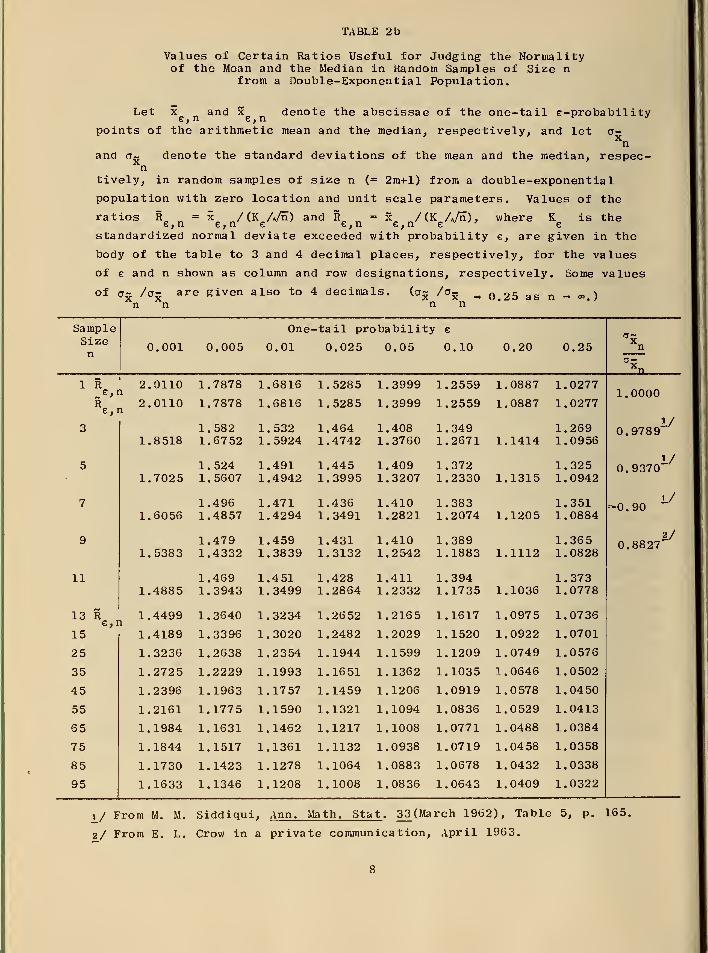
TABLE 2b

Values of Certain Ratios Useful for Judging the Normalityof the Mean and the Median in Random Samples of Size n

from a Double-Exponential Population.

Let x and x denote the abscissae of the one-tail e-probability

points of the arithmetic mean and the median, respectively, and let tr-xnand cr~ denote the standard deviations of the mean and the median, respec-

ntively, in random samples of size n (= 2ra+l) from a double-exponential

population with zero location and unit scale parameters. Values of the

ratios Re, n

= xg, n

/(K A/n) and Re, n

x_ /(K A/iT), where K is the

standardized normal deviate exceeded with probability e, are given in the

body of the table to 3 and 4 decimal places, respectively, for the values

of e and n shown as column and row designations, respectively. Some values

of o~ /g- are given also to 4 decimals. (a~ /a- _, Q>25 as n _ w# )n n n n

SampleSizen

0.001 0.005

One

0.01

-tail probability e

0.025 0.05 0.10 0.20 0.25

1 it

E«,«

2.0110l

2.0110l

1.7878

1.7878

1.6816

1.6816

1.5285

1.5285

1.3999

1.3999

1.2559

1.2559

1.0887

1.0887

1.0277

1.02771.0000

31.8518

1.5821.6752

1.5321.5924

1.4641.4742

1.4081.3760

1.3491.2671 1.1414

1.2691.0956

1/0.9789

51.7025

1.5241 . 5607

1.4911.4942

1.4451.3995

1.4091.3207

1.3721.2330 1.1315

1.3251.0942

1/0.9370

7

1.60561.4961.4857

1.4711.4294

1.4361.3491

1.4101.2821

1.3831.2074 1.1205

1.3511.0884

~0.90

9

1.53831.4791.4332

1.4591.3839

1.4311.3132

1.4101.2542

1.3891.1883 1.1112

1.3651.0828

2/0.8827

111.4885

1.4691.3943

1.4511.3499

1.4281.2864

1.4111.2332

1.3941.1735 1.1036

1.3731.0778

13 RG . I

1.4499 1.3640 1.3234 1.2652 1.2165 1.1617 1.0975 1.0736

15^ >

1.4189 1.3396 1.3020 1.2482 1.2029 1.1520 1.0922 1.0701

25 1.3236 1.2638 1.2354 1.1944 1.1599 1.1209 1.0749 1.0576

35 1.2725 1.2229 1.1993 1.1651 1.1362 1.1035 1.0646 1.0502

45 1.2396 1.1963 1.1757 1.1459 1.1206 1.0919 1.0578 1.0450

55 1.2161 1.1775 1.1590 1.1321 1.1094 1.0836 1.0529 1.0413

65 1.1984 1.1631 1.1462 1.1217 1.1008 1.0771 1.0488 1.0384

75 1.1844 1.1517 1.1361 1.1132 1.0938 1.0719 1.0458 1.0358

85 1.1730 1.1423 1.1278 1.1064 1.0883 1.0678 1.0432 1.0338

95 1.1633 1.1346 1.1208 1.1008 1.0836 1.0643 1.0409 1.0322

i_/ From M. M. Siddiqui, Ann. Math. Stat . 33_(March 1962), Table 5, p. 165.

2/ From E. L. Crow in a private communication, April 1963.

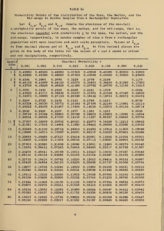
TABLE 3a

Probability Points of the Distribution of the Mean, the Median, and theMid-Range in Random Samples from a Rectangular Population

Let x , x and x denote the abscissae of the one-taile,n' e, n e, n

e-probability points of the mean, the median, and the mid-range, that is,

the abscissae exceeded with probability e_ by the mean, the median, and the

mid-range, respectively, in random samples of size n from a rectangular

population with zero location and unit scale parameters. Values of xs • n

to four decimal places and of 5L and x to five decimal places areg, n e, n

given in the body of the table for the values of e and n shown as column

and row designations, respectively.

SampleSizen

0.001 0.005

One-tail Probability e

0.010 0.025 0.050 0.100 0.200 0.250T

1 XX

3 xXX

11 XX

13

15

25

35

45

55

65

75

85

95

0.499000.49900

0.43940.481630.43700

0.36910.452450.35573

0.32000.423340.29422

0.28580.397480.24934

0.375070.21581

0.355690.19000

0.338830.16960

0.279350.11005

0.242780.08134

0.217530.06450

0.198770.05342

0.184150.04559

0.172340.03976

0.162540.03525

0.154230.03166

0.495000.49500

0.39640.458600.39228

0.31940.417170.30095

0.27320.382300.24103

0.24260.353940.20026

0.330690.17103

0.311300.14915

0.294860.13218

0.239260.08412

0.206410.06164

0.184160.04864

0.167830.04016

0.155180.03420

0.145020.02978

0.136620.02637

0.129530.02366

0.490000.49000

0.36950.441100.36428

0.29260.394360.27135

0.24920.357730.21407

0.22070.329030.17626

0.306020.14964

0.287120.12993

0.271270.11478

0.218590.07243

0.187990.05288

0.167420.04163

0.152400.03433

0.140800.02920

0.131500.02541

0.123820.02249

0.117360.02017

0.475000.47500

0.32290.405700.31580

0.25080.353370.22536

0.21250.315950.17408

0.18770.287990.14156

0.266210.11920

0.248650.10291

0.234140.09052

0.186940.05646

0.160110.04102

0.142260.03220

0.129290.02651

0.119330.02252

0.111360.01958

0.104800.01732

0.099280.01552

0.450000.45000

0.27690.364650.26792

0.21310.310740.18452

0.17990.274680.14016

0.15850.248630.11287

0.228750.09443

0.212950.08116

0.200010.07115

0.158610.04400

0.135430.03184

0.120130.02494

0.109060.02050

0.100580.01740

0.093790.01512

0.088240.01336

0.083560.01197

0.400000.40000

0.21890.304200.20760

0.16790.253360.13761

0.14130.221400.10270

0.12430.199030.08187

0.182280.06806

0.169140.05822

0.158480.05087

0.124860.03117

0.106310.02247

0.094140.017 57

0.085380.01442

0.078680.01223

0.073340.01062

0.068970.00938

0.065290.00840

0.300000.30000

0.212860.13160

0.173400.08372

0.149910.06135

0.133910.04840

0.122130.03996

0.113000.03403

0.105640.02963

0.082750.01799

0.070270.01292

0.062140.01008

0.056310.00826

0.051850.00700

0.048320.00607

0.045420.00536

0.042980.00480

0.250000.25000

0.11760.173650.10315

0.08940.140560.06472

0.07500.121150.04714

0.06580.108040.03706

0.098420.03053

0.090980.02596

0.085010.02258

0.066480.01367

0.056420.00980

0.049870.00764

0.045180.00626

0.041600.00530

0.0387 50.00460

0.036420.00406

0.034470.00363

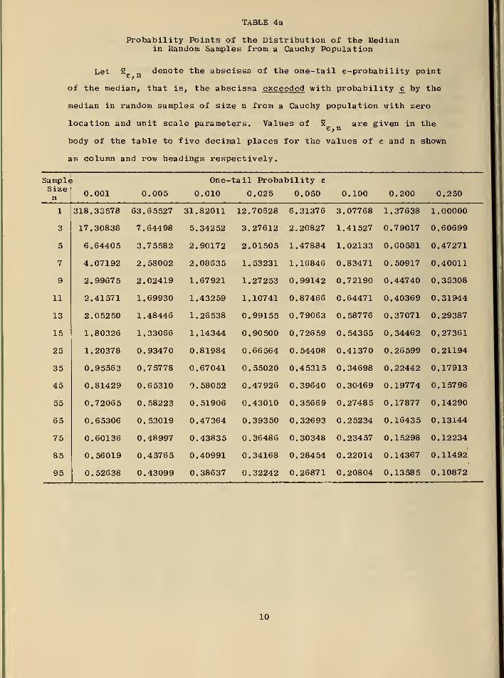
TABLE 4a

Probability Points of the Distribution of the Medianin Random Samples from a Cauchy Population

Let x denote the abscissa of the one-tail e-probability point

of the median, that is, the abscissa exceeded with probability e^ by the

median in random samples of size n from a Cauchy population with zero

location and unit scale parameters. Values of x are given in thee, n °

body of the table to five decimal places for the values of e and n shown

as column and row headings respectively.

Sample 1 One- tail Probability e

Sizen 0.001 0.005 0.010 0.025 0.050 0.100 0.200 0.250

1 318.33578 63.85527 31.82011 12.70628 6.31376 3.07768 1.37638 1.00000

3 17.30838 7.64498 5.34252 3.27612 2.20827 1.41527 0.79017 0.60699

5 6.64405 3.75582 2.90172 2.01505 1.47884 1.02133 0.60581 0.47271

7 4.07192 2.58002 2.08635 1.53231 1.16846 0.83471 0.50917 0.40011

9 2.99675 2.02419 1.67921 1.27253 0.99142 0.72190 0.44740 0.35308

11 2.41571 1.69930 1.43259 1.10741 0.87466 0.64471 0.40369 0.31944

13 2.05250 1.48446 1.26538 0.99155 0.79063 0.58776 0.37071 0.29387

15 1.80326 1.33066 1.14344 0.90500 0.72659 0.54355 0.34462 0.27361

25 1.20378 0.93470 0.81984 0.66564 0.54408 0.41370 0.26599 0.21194

35 0.95563 0.75778 0.67041 0.55020 0.45315 0.34698 0.22442 0.17913

45 0.81429 0.65310 0.58052 0.47926 0.39640 0.30469 0.19774 0.15796

55 0.72065 0.58223 0.51906 0.43010 0.35669 0.27485 0.17877 0.14290

65 0.65306 0.53019 0.47364 0.39350 0.32693 0.25234 0.16435 0.13144

75 0.60136 0.48997 0.43835 0.36486 0.30348 0.23457 0.15298 0.12234

85 0.56019 0.45765 0.40991 0.34168 0.28454 0.22014 0.14367 0.11492

95 0.52638 0.43099 0.38637 0.32242 0.26871 0.20804 0.13585 0.10872

10

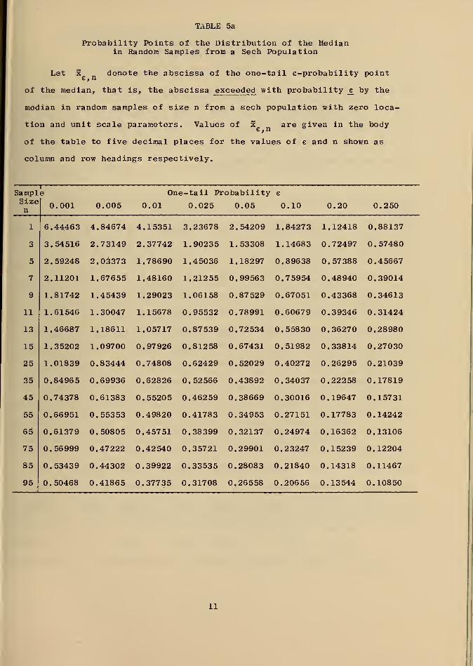
TABLE 5a

Probability Points of the Distribution of the Medianin Random Samples from a Sech Population

Let x denote the abscissa of the one-tail e-probability point

of the median, that is, the abscissa exceeded with probability _e by the

median in random samples of size n from a sech population with zero loca-

tion and unit scale parameters. Values of x are given in the body

of the table to five decimal places for the values of e and n shown as

column and row headings respectively.

SamplT

e One-tail Probability e

Sizen

0.001 0.005 0.01 0.025 0.05 0.10 0.20 0.250

1 6.44463 4.84674 4.15351 3.23678 2.54209 1.84273 1.12418 0.88137

3 3.54516 2.73149 2.37742 1.90235 1.53308 1.14683 0.72497 0.57480

5 2.59248 2.03373 1.78690 1.45036 1.18297 0.89638 0.57388 0.45667

7 2.11201 1.67655 1.48160 1.21255 0.99563 0.75954 0.48940 0.39014

9 1.81742 1.45439 1.29023 1.06158 0.87 529 0.67051 0.43368 0.34613

11 1.61546 1.30047 1.15678 0.95532 0.78991 0.60679 0.39346 0.31424

13 1.46687 1.18611 1.05717 0.87539 0.72534 0.55830 0.36270 0.28980

15 1.35202 1.09700 0.97926 0.81258 0.67431 0.51982 0.33814 0.27030

25 1.01839 0.83444 0.74808 0.62429 0.52029 0.40272 0.26295 0.21039

35 0.84965 0.69936 0.62826 0.52566 0.43892 0.34037 0.22258 0.17819

45 0.74378 0.61383 0.55205 0.46259 0.38669 0.30016 0.19647 0.15731

55 0.66951 0.55353 0.49820 0.41783 0.34953 0.27151 0.17783 0.14242

65 0.61379 0.50805 0.45751 0.38399 0.32137 0.24974 0.16362 0.13106

75 0.56999 0.47222 0.42540 0.35721 0.29901 0.23247 0.15239 0.12204

85 0.53439 0.44302 0.39922 0.33535 0.28083 0.21840 0.14318 0.11467

95 0.50468 0.41865 0.37735 0.31708 0.26558 0.20656 0.13544 0.10850

11

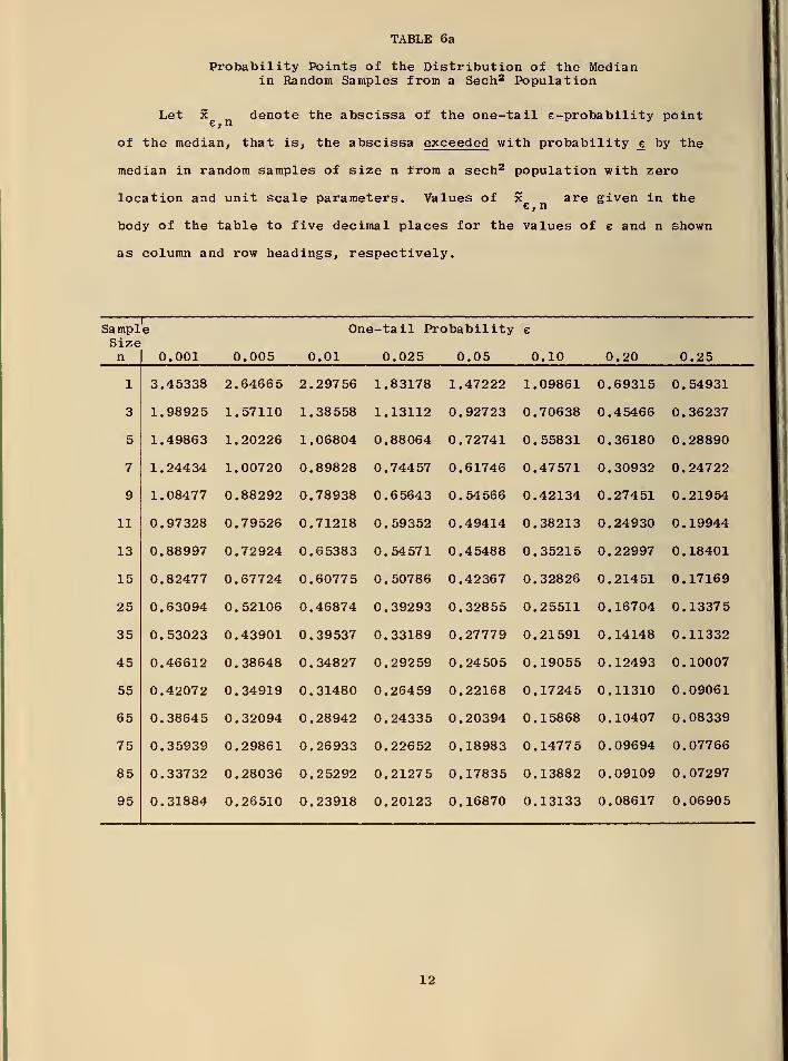
TABLE 6a

Probability Points of the Distribution of the Medianin Random Samples from a Sech2 Population

Let x denote the abscissa of the one-tail e-probability point

of the median, that is, the abscissa exceeded with probability e by the

median in random samples of size n from a sech2 population with zero

location and unit scale parameters. Values of x are given in the

body of the table to five decimal places for the values of e and n shown

as column and row headings, respectively.

SamplSizen

e

0.001 0.005

One-tail Probability

0.01 0.025 0.05

c

0.10 0.20 0.25

1 3.45338 2.64665 2.297 56 1.83178 1.47222 1.09861 0.69315 0.54931

3 1.98925 1.57110 1.38558 1.13112 0.92723 0.70638 0.45466 0.36237

5 1.49863 1.20226 1.06804 0.88064 0.72741 0.55831 0.36180 0.28890

7 1.24434 1.00720 0.89828 0.74457 0.61746 0.47571 0.30932 0.24722

9 1.08477 0.88292 0.78938 0.65643 0.54566 0.42134 0.27451 0.21954

11 0.97328 0.79526 0.71218 0.59352 0.49414 0.38213 0.24930 0.19944

13 0.88997 0.72924 0.65383 0.54571 0.45488 0.35215 0.22997 0.18401

15 0.82477 0.67724 0.60775 0.50786 0.42367 0.32826 0.21451 0.17169

25 0.63094 0.52106 0.46874 0.39293 0.32855 0.25511 0.16704 0.13375

35 0.53023 0.43901 0.39537 0.33189 0.27779 0.21591 0.14148 0.11332

45 0.46612 0.38648 0.34827 0.29259 0.24505 0.19055 0.12493 0.10007

55 0.42072 0.34919 0.31480 0.26459 0.22168 0.17245 0.11310 0.09061

65 0.38645 0.32094 0.28942 0.24335 0.20394 0.15868 0.10407 0.08339

75 0.35939 0.29861 0.26933 0.22652 0.18983 0.14775 0.09694 0.07766

85 0.33732 0.28036 0.25292 0.21275 0.17835 0.13882 0.09109 0.07297

95 0.31884 0.26510 0.23918 0.20123 0.16870 0.13133 0.08617 0.06905

12

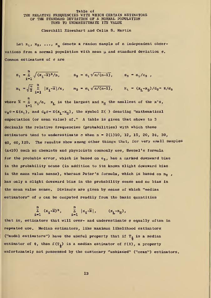
Table ofTHE RELATIVE FREQUENCIES WITH WHICH CERTAIN ESTIMATORS

OF THE STANDARD DEVIATION OF A NORMAL POPULATIONTEND TO UNDERESTIMATE ITS VALUE

Churchill Eisenhart and Celia S. Martin

Let xr , x2 , . .., x denote a random sample of n independent obser-

vations from a normal population with mean \i and standard deviation <j.

Common estimators of <r are

n2i=l

n .

l- 2

1/(x

i-x) 2/n, s 2 - s

xi/n/(n-l), s 3 = s

x /c2 ,

n

^ 2 |x±-x|/n, m2 = m

1 i/n/(n-l), Rt

- (xL-x

g)/d2

= R/d 2

nwhere x = 2 x./n, xT is the largest and xa the smallest of the x's,

i-1i L s

c 2o = E(s

1 ), and d2 o= E(xL-xg ) , the symbol E( ) denoting "mathematical

expectation (or mean value) of." A table is given that shows to 3

decimals the relative frequencies (probabilities) with which these

estimators tend to underestimate a when n - 2(1)10, 12, 15, 20, 24, 30,

40 60 120. The results show among other things that, for very small samples

(nslO) such as chemists and physicists commonly use, Bessel's formula

for the probable error, which is based on s 2 , has a marked downward bias

in the probability sense (in addition to its known slight downward bias

in the mean value sense), whereas Peter's formula, which is based on m2 ,

has only a slight downward bias in the probability sense and no bias in

the mean value sense. Divisors are given by means of which "median

estimators" of a can be computed readily from the basic quantities

n n2 (x.-x)2, z |x.-x|, (x.-x ),i-1

xi-1

x u b

that is, estimators that will over- and underestimate a equally often in

repeated use. Median estimators, like maximum likelihood estimators

("modal estimators") have the useful property that if Ti is a median

estimator of G, then f (TO is a median estimator of f(9), a property

unfortunately not possessed by the customary "unbiased" ("mean") estimators.

13

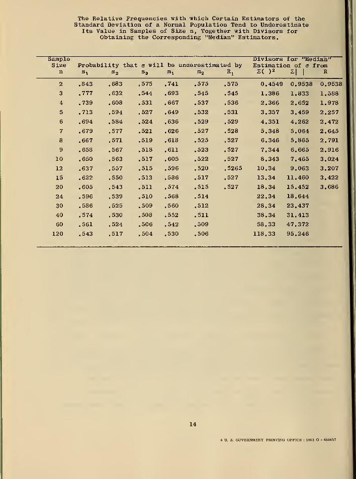
The Relative Frequencies with which Certain Estimators of theStandard Deviation of a Normal Population Tend to Underestimate

Its Value in Samples of Size n, Together with Divisors forObtaining the Corresponding "Median" Estimators.

Sample"

Size Probability that a will be underestimated byn s, s» s, m, rrio R,

Divisors for "Median'Estimation of o from2( )

22|

|

R

2 .843 .683 .575 .741 .575 .575 0.4549 0.9538 0.9538

3 .777 .632 .544 .693 .545 .545 1.386 1.833 1.588

4 .739 .608 .531 .667 .537 .536 2.366 2.652 1.978

5 .713 .594 .527 .649 .532 .531 3.357 3.459 2.257

6 .694 .584 .524 .636 .529 .529 4.351 4.262 2.472

7 .679 .577 .521 .626 .527 .528 5.348 5.064 2.645

8 .667 .571 .519 .618 .525 .527 6.346 5.865 2.791

9 .658 .567 .518 .611 .523 .527 7.344 6.665 2.916

10 .650 .563 .517 .605 .522 .527 8.343 7.465 3.024

12 .637 .557 .515 .596 .520 .5265 10.34 9.063 3.207

15 .622 .550 .513 .586 .517 .527 13.34 11.460 3.422

20 .605 .543 .511 .574 .515 .527 18.34 15.452 3.686

24 .596 .539 .510 .568 .514 22.34 18.644

30 .586 .525 .509 .560 .512 28.34 23.437

40 .574 .530 .508 .552 .511 38.34 31.413

60 .561 .524 .506 .542 .509 58.33 47.372

120 .543 .517 .504 .530 .506 118.33 95.246

14

ft U. S. GOVERNMENT PRINTING OFFICE : 1963 O - 688657

U. S. DEPARTMENT OF COMMERCELuther H. Hodges, Secretary

NATIONAL BUREAU OF STANDARDSA. V. Astin, Director

THE NATIONAL BUREAU OF STANDARDS

The scope of activities of the National Bureau of Standards at its major laboratories in Washington, D.C.andBoulder, Colorado, is suggested in the following listing of the divisions and sections engaged in technical work.In general, each section carries out specialized research, development, and engineeringin the field indicated byits title. A brief description of the activities, and of the resultant publications, appears on the inside of thefront cover.

WASHINGTON. II. C.

Electricity. Resistance and Reactance. Electrochemistry. Electrical Instruments. Magnetic Measurements.Dielectrics. High Voltage. Absolute Electrical Measurements.

Metrology. Photometry and Colorimetry. Refractometry. Photographic Research. Length. Engineering Metrology.Mass and Volume.

Heat. Temperature Physics. Heat Measurements. Cryogenic Physics. Equation of State. Statistical Physics.

Radiation Physics. X-ray. Radioactivity. Radiation Theory. High Energy Radiation. Radiological Equipment.

Nuclronic Instrumentation. Neutron Physics.

Analytical and Inorganic Chemistry. Pure Substances. Spectrochemistry. Solution Chemistry. Standard Refer-

ence Materials. Applied Analytical Research. Crystal Chemistry.

Mechanics. Sound. Pressure and Vacuum. Fluid Mechanics. Engineering Mechanics. Rheology. CombustionControls.

Polymers. Macromolecules: Synthesis and Structure. Polymer Chemistry. Polymer Physics. Polymer Charac-terization. Polymer Evaluation and Testing. Applied Polymer Standards and Research. Dental Research.

Metallurgy. Engineering Metallurgy. Metal Reactions. Metal Physics. Electrolysis and Metal Deposition.

Inorganic Solids. Engineering Ceramics. Class. Solid State Chemistry. Crystal Growth. Physical Properties.

Crystallography.

Building Research. Structural Engineering. Fire Research. Mechanical Systems. Organic Building Materials.

Codes and Safely Standards. Heat Transfer. Inorganic Building Materials. Metallic Building Materials.

Applied Mathematics. Numerical Analysis. Computation. Statistical Engineering. Mathematical Physics. Op-erations Research.

Data Processing Systems. Components and Techniques. Computer Technology. Measurements Automation.

Engineering Applications. Systems Analysis.

Atomic Physics. Spectroscopy. Infrared Spectroscopy. Far Ultraviolet Physics. Solid State Physics. ElectronPhysics. Atomic Physics. Plasma Spectroscopy.

Instrumentation. Engineering Electronics. Electron Devices. Electronic Instrumentation. Mechanical Instru-

ments. Basic Instrumentation.

Physical Chemistry. Thermochemistry. Surface Chemistry. Organic Chemistry. Molecular Spectroscopy. Ele-

mentary Processes. Mass Spectrometry. Photochemistry and Radiation Chemistry.

Office of Weights and Measures.

BOULDER, COLO.

CRYOGENIC ENGINEERING LABORATORY

Cryogenic Processes. Cryogenic Properties of Solids. Cryogenic Technical Services. Properties of CryogenicFluids.

CENTRAL RADIO PROPAGATION LABORATORY

Ionosphere Research and Propagation. Low Frequency and Very Low Frequency Research. Ionosphere Re-search. Prediction. Services. Sun-Earth Relationships. Field Engineering. Radio Warning Services. VerticalSoundings Research.

Troposphere and Space Telecommunications. Data Reduction Instrumentation. Radio Noise. Tropospheric

Measurements. Tropospheric Analysis. Spectrum Utilization Research. Radio-Meteorology. Lower AtmospherePhysics.

Radio Systems. Applied Electromagnetic Theory. High Frequency and Very High Frequency Research. Fre-

quency Utilization. Modulation Research. Antenna Research. Radiodetermination.

Upper Atmosphere and Space Physics. Upper Atmosphere and Plasma Physics. High Latitude IonospherePhysics. Ionosphere and Exosphere Scatter. Airglow and Aurora. Ionospheric Radio Astronomy.

RADIO STANDARDS LABORATORY

Radio Standards Physics. Frequency and Time Disseminations. Radio and Microwave Materials. Atomic Fre-

quency and Time-Interval Standards. Radio Plasma. Microwave Physics.

Radio Standards Engineering. High Frequency Electrical Standards. High Frequency Calibration Services. HighFrequency Impedance Standards. Microwave Calibration Services. Microwave Circuit Standards. Low FrequencyCalibration Services.

Joint Institute for Laboratory Astrophysics -NBS Group (Univ. of Colo.).

NBS