Tables and Priority Queues - Simon Fraser · PDF filefor a min heap. Complete Binary ......
54
Tables and Priority Queues
-
Upload
vuongduong -
Category
Documents
-
view
221 -
download
1
Transcript of Tables and Priority Queues - Simon Fraser · PDF filefor a min heap. Complete Binary ......
Tables and Priority Queues
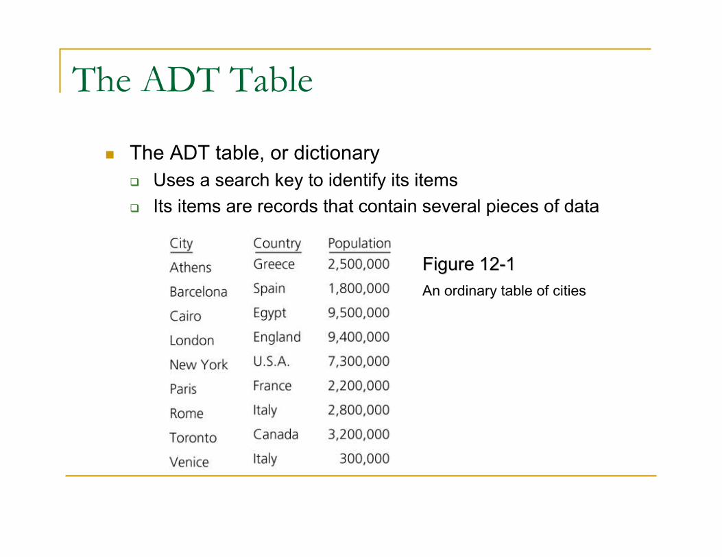
The ADT Table
� The ADT table, or dictionary
� Uses a search key to identify its items
� Its items are records that contain several pieces of data
Figure 12Figure 12--11
An ordinary table of cities
The ADT Table
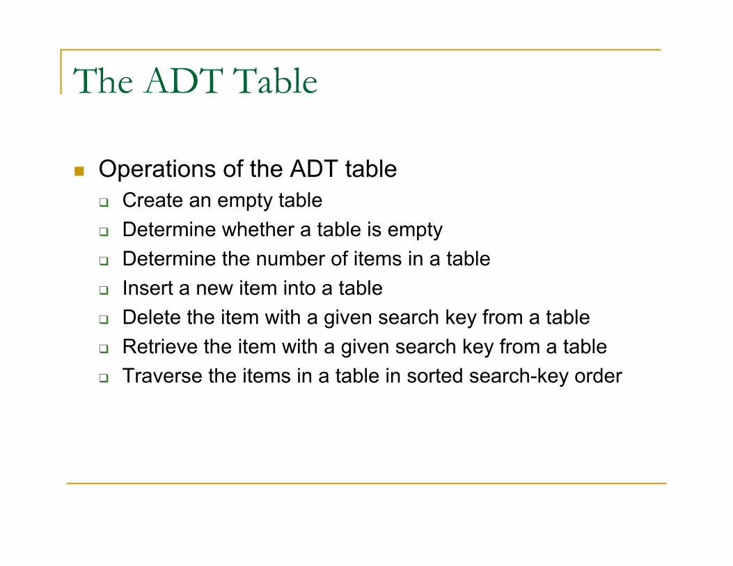
� Operations of the ADT table
� Create an empty table
� Determine whether a table is empty
� Determine the number of items in a table
� Insert a new item into a table
� Delete the item with a given search key from a table
� Retrieve the item with a given search key from a table
� Traverse the items in a table in sorted search-key order
The ADT Table
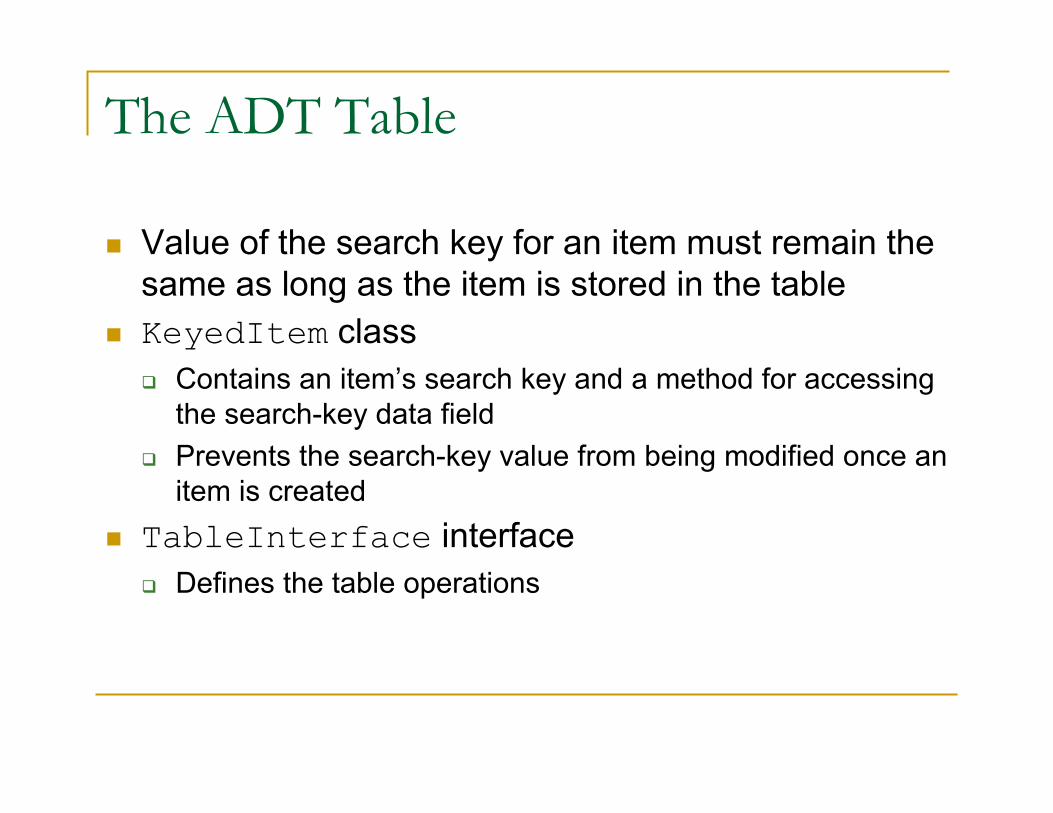
� Value of the search key for an item must remain the
same as long as the item is stored in the table
� KeyedItem class
� Contains an item’s search key and a method for accessing
the search-key data field
� Prevents the search-key value from being modified once an
item is created
� TableInterface interface
� Defines the table operations
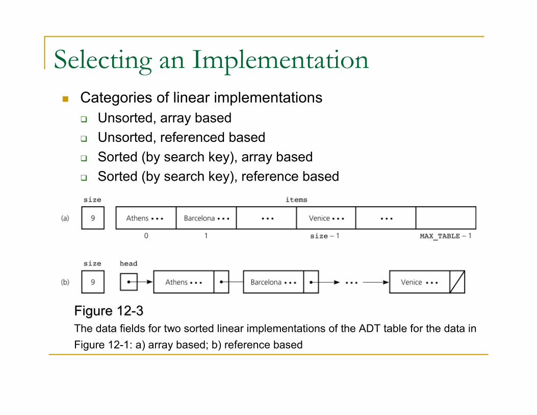
Selecting an Implementation
� Categories of linear implementations
� Unsorted, array based
� Unsorted, referenced based
� Sorted (by search key), array based
� Sorted (by search key), reference based
Figure 12Figure 12--33
The data fields for two sorted linear implementations of the ADT table for the data in
Figure 12-1: a) array based; b) reference based
Selecting an Implementation
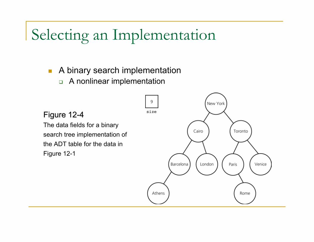
� A binary search implementation
� A nonlinear implementation
Figure 12Figure 12--44
The data fields for a binary
search tree implementation of
the ADT table for the data in
Figure 12-1
Selecting an Implementation
� The binary search tree implementation offers several advantages over linear implementations
� The requirements of a particular application influence the selection of an implementation� Questions to be considered about an application before
choosing an implementation
� What operations are needed?
� How often is each operation required?
Scenario A: Insertion and Traversal in No
Particular Order
� An unsorted order is efficient� Both array based and reference based tableInsert
operation is O(1)
� Array based versus reference based� If a good estimate of the maximum possible size of the
table is not available
� Reference based implementation is preferred
� If a good estimate of the maximum possible size of the table is available
� The choice is mostly a matter of style
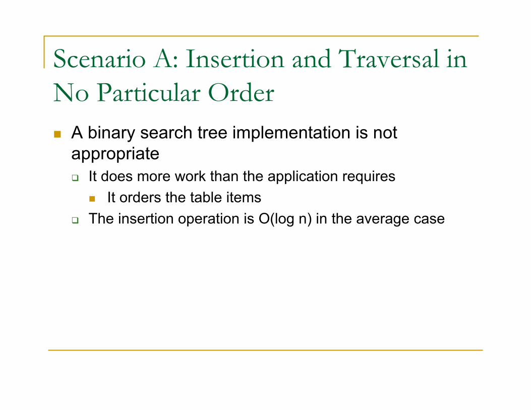
Scenario A: Insertion and Traversal in
No Particular Order
� A binary search tree implementation is not
appropriate
� It does more work than the application requires
� It orders the table items
� The insertion operation is O(log n) in the average case
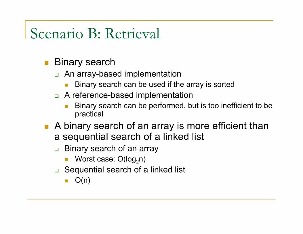
Scenario B: Retrieval
� Binary search� An array-based implementation
� Binary search can be used if the array is sorted
� A reference-based implementation
� Binary search can be performed, but is too inefficient to be practical
� A binary search of an array is more efficient than a sequential search of a linked list� Binary search of an array
� Worst case: O(log2n)
� Sequential search of a linked list
� O(n)
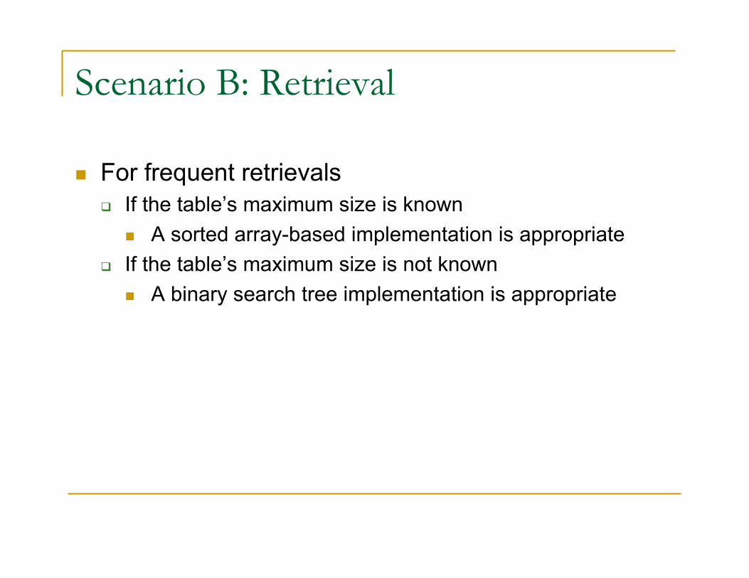
Scenario B: Retrieval
� For frequent retrievals
� If the table’s maximum size is known
� A sorted array-based implementation is appropriate
� If the table’s maximum size is not known
� A binary search tree implementation is appropriate
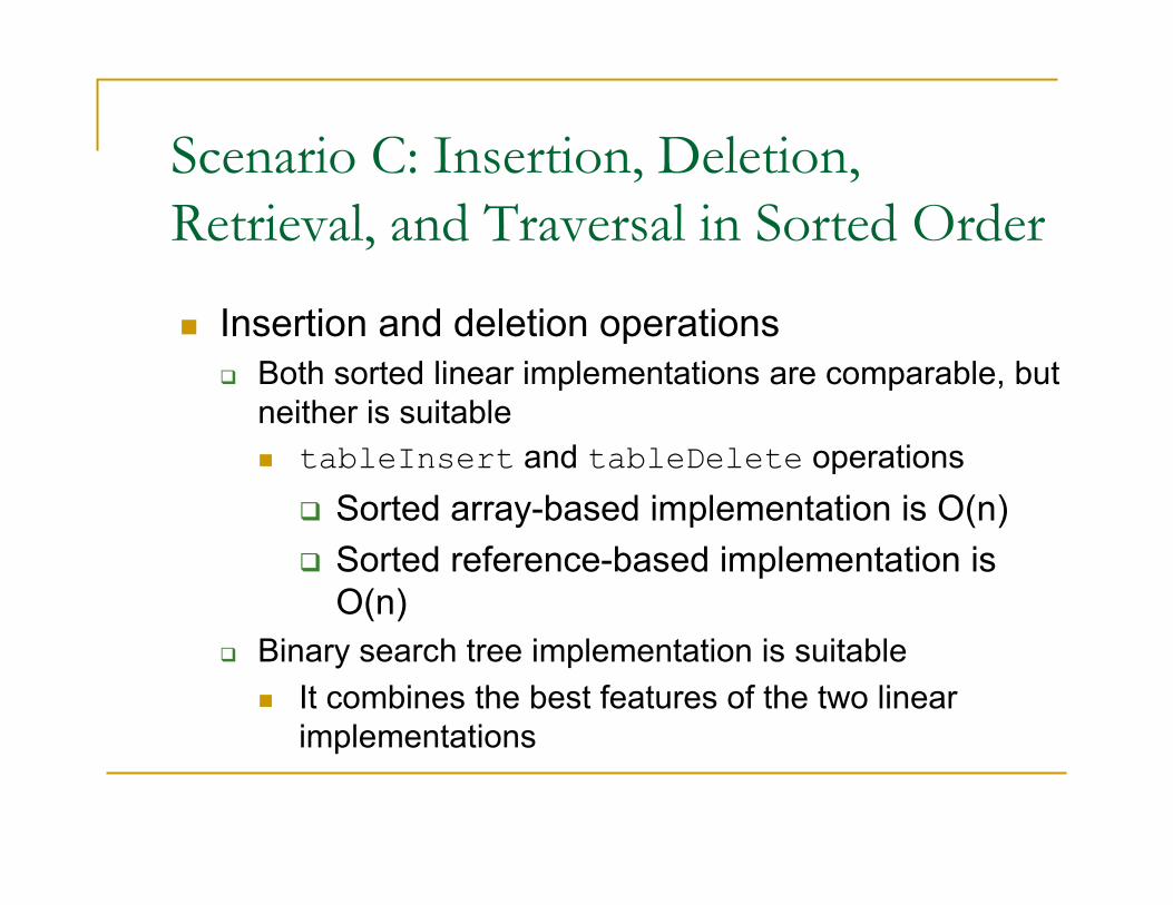
Scenario C: Insertion, Deletion,
Retrieval, and Traversal in Sorted Order
� Insertion and deletion operations
� Both sorted linear implementations are comparable, but
neither is suitable
� tableInsert and tableDelete operations
� Sorted array-based implementation is O(n)
� Sorted reference-based implementation is
O(n)
� Binary search tree implementation is suitable
� It combines the best features of the two linear
implementations
A Sorted Array-Based Implementation
of the ADT Table
� Linear implementations
� Useful for many applications despite certain difficulties
� A binary search tree implementation
� In general, can be a better choice than a linear
implementation
� A balanced binary search tree implementation
� Increases the efficiency of the ADT table operations
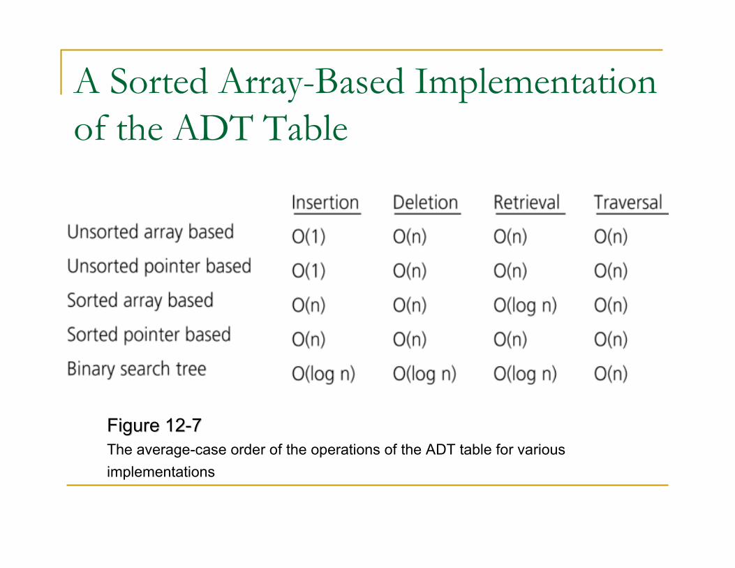
A Sorted Array-Based Implementation
of the ADT Table
Figure 12Figure 12--77
The average-case order of the operations of the ADT table for various
implementations
Priority Queue
The ADT Priority Queue:
A Variation of the ADT Table
� The ADT priority queue� Orders its items by a priority value
� The first item removed is the one having the highest priority value
� Operations of the ADT priority queue� Create an empty priority queue
� Determine whether a priority queue is empty
� Insert a new item into a priority queue
� Retrieve and then delete the item in a priority queue with the highest priority value
The ADT Priority Queue:
A Variation of the ADT Table� Pseudocode for the operations of the ADT priority
queuecreatePQueue()
// Creates an empty priority queue.
pqIsEmpty()
// Determines whether a priority queue is
// empty.
The ADT Priority Queue:
A Variation of the ADT Table� Pseudocode for the operations of the ADT priority queue (Continued)pqInsert(newItem) throws PQueueException
// Inserts newItem into a priority queue.
// Throws PQueueException if priority queue is
// full.
pqDelete()
// Retrieves and then deletes the item in a
// priority queue with the highest priority
// value.
The ADT Priority Queue:
A Variation of the ADT Table� Possible implementations
� Sorted linear implementations
� Appropriate if the number of items in the priority queue is small
� Array-based implementation
� Maintains the items sorted in ascending order of priority value
� Reference-based implementation
� Maintains the items sorted in descending order of priority value
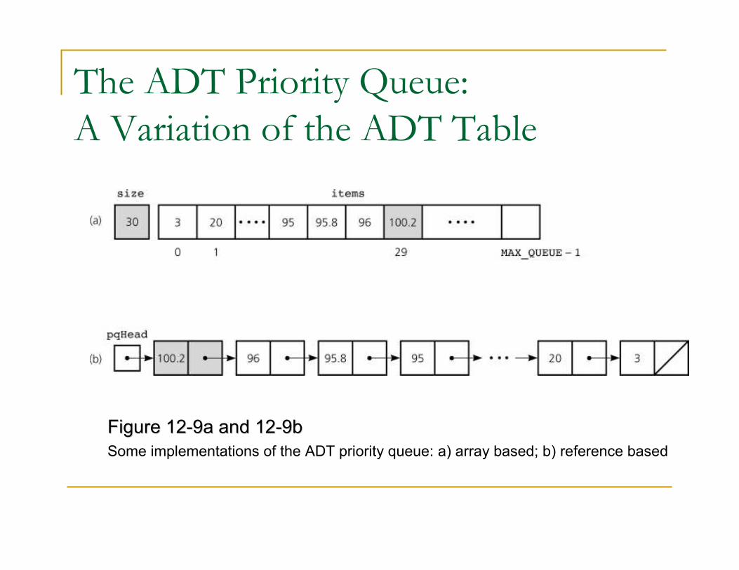
The ADT Priority Queue:
A Variation of the ADT Table
Figure 12Figure 12--9a and 129a and 12--9b9b
Some implementations of the ADT priority queue: a) array based; b) reference based
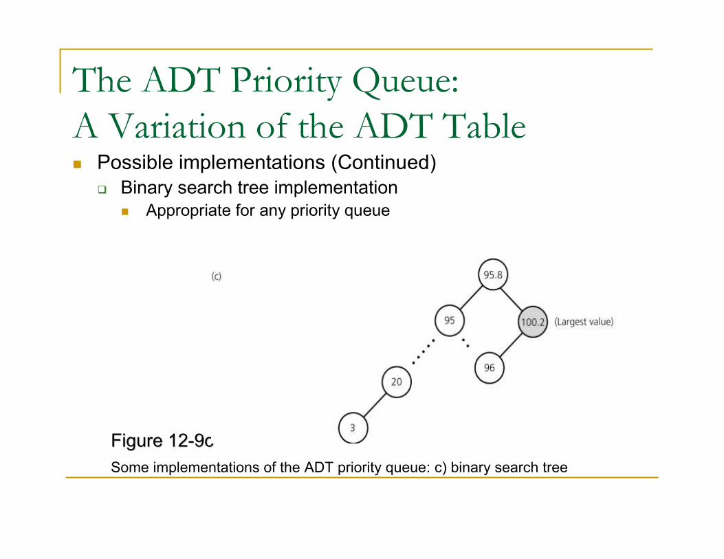
The ADT Priority Queue:
A Variation of the ADT Table� Possible implementations (Continued)
� Binary search tree implementation
� Appropriate for any priority queue
Figure 12Figure 12--9c9c
Some implementations of the ADT priority queue: c) binary search tree
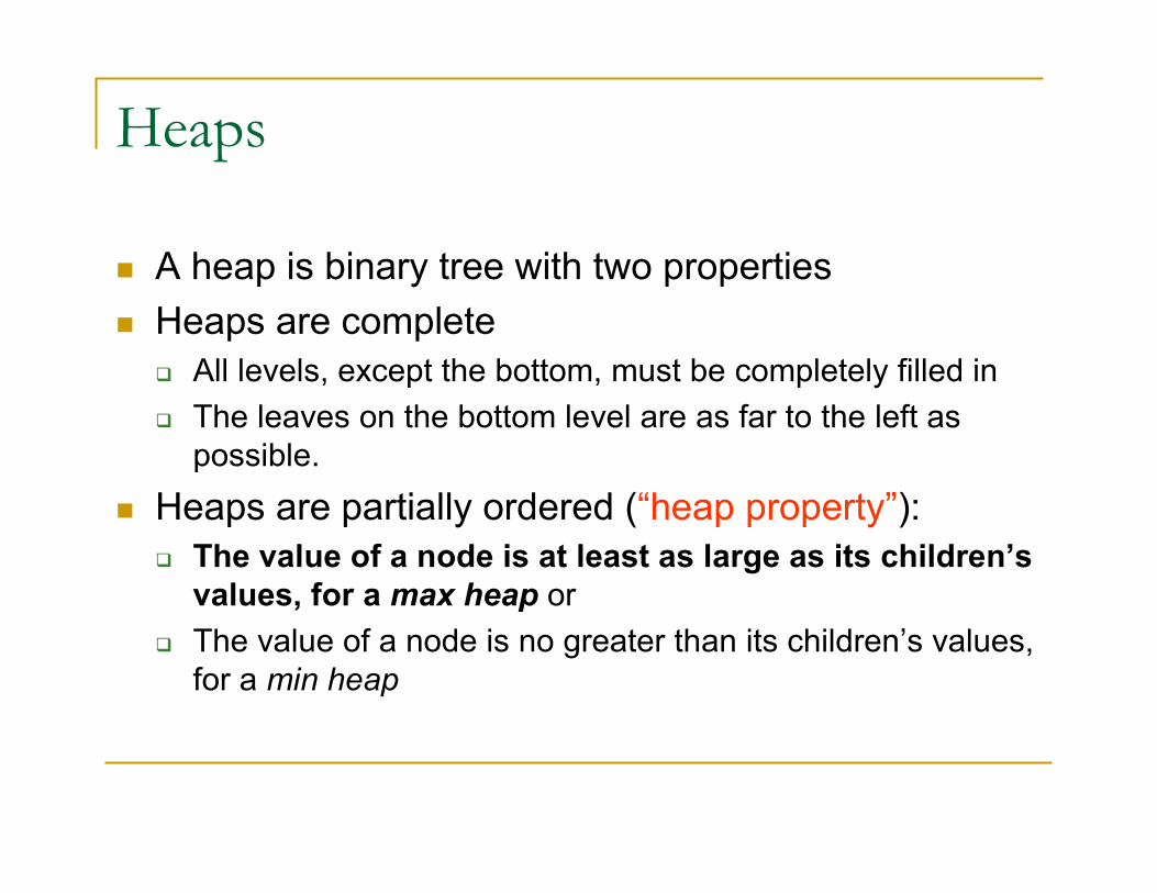
Heaps
� A heap is binary tree with two properties
� Heaps are complete
� All levels, except the bottom, must be completely filled in
� The leaves on the bottom level are as far to the left as
possible.
� Heaps are partially ordered (“heap property”):
� The value of a node is at least as large as its children’s
values, for a max heap or
� The value of a node is no greater than its children’s values,
for a min heap
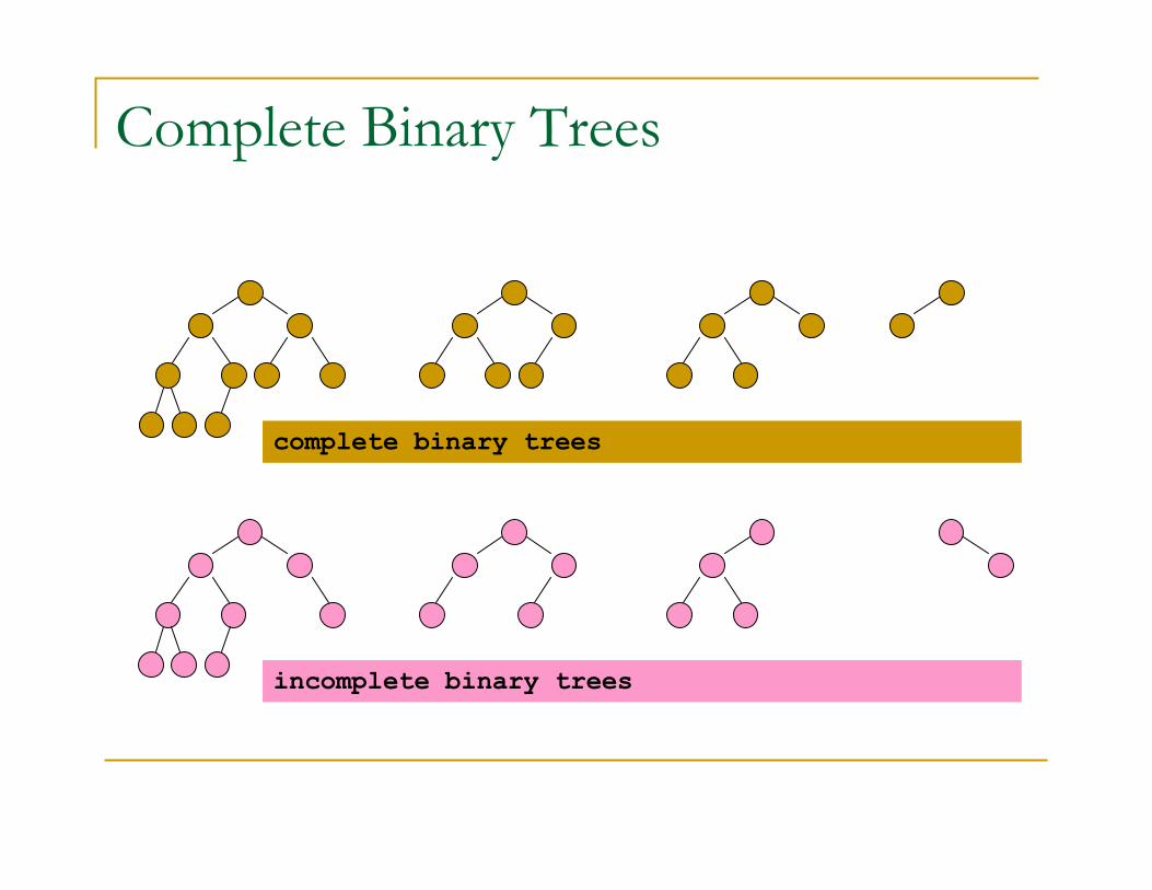
Complete Binary Trees
complete binary trees
incomplete binary trees
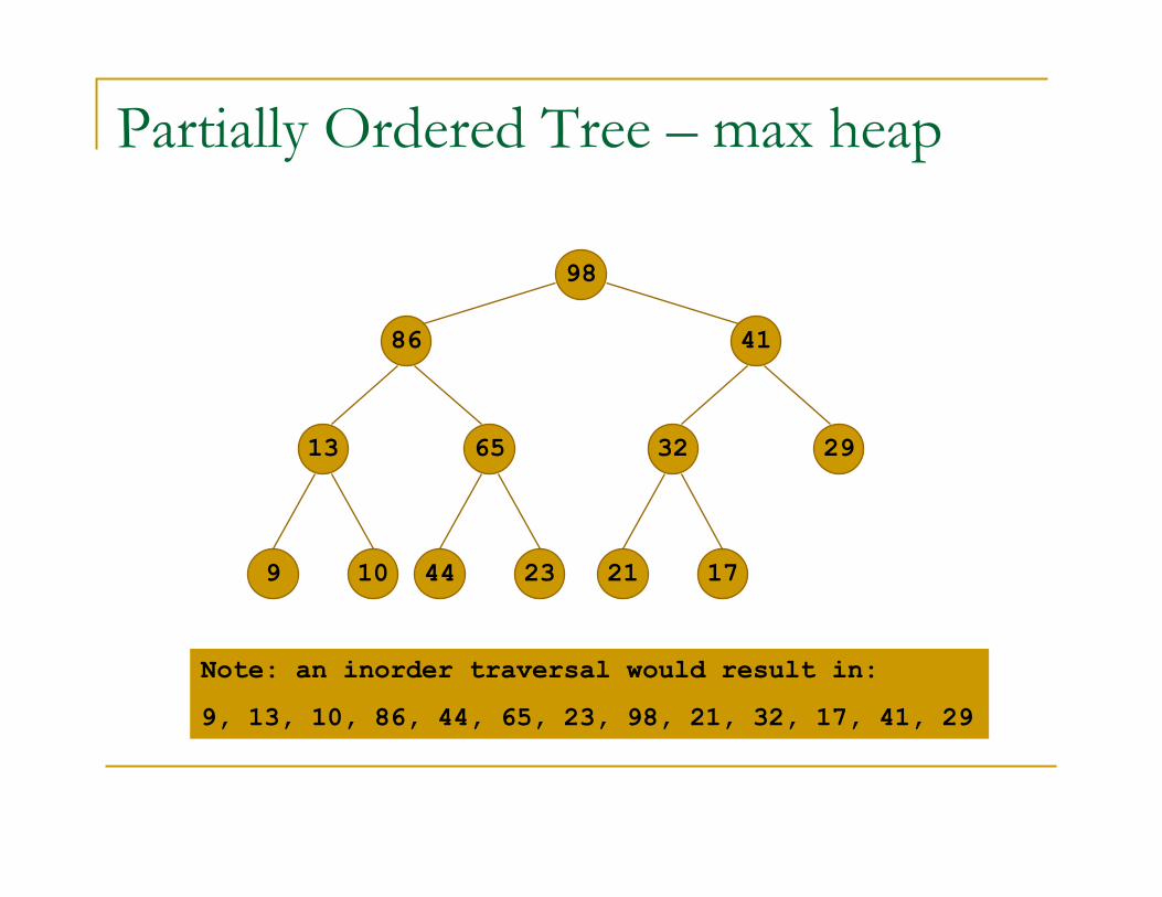
Partially Ordered Tree – max heap
98
4186
13 65
9 10
32 29
44 23 21 17
Note: an inorder traversal would result in:
9, 13, 10, 86, 44, 65, 23, 98, 21, 32, 17, 41, 29
Priority Queues and Heaps
� A heap can be used to implement a priority queue
� Because of the partial ordering property the item at the top of the heap must always the largest value
� Implement priority queue operations:� Insertions – insert an item into a heap
� Removal – remove and return the heap’s root
� For both operations preserve the heap property
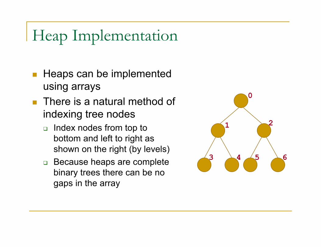
Heap Implementation
� Heaps can be implemented
using arrays
� There is a natural method of
indexing tree nodes
� Index nodes from top to
bottom and left to right as
shown on the right (by levels)
� Because heaps are complete
binary trees there can be no
gaps in the array
0
1 2
3 4 5 6
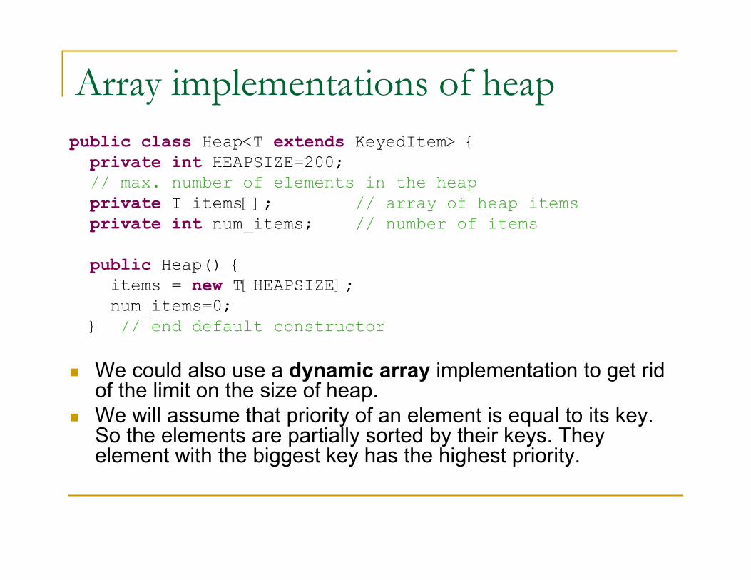
Array implementations of heap
public class Heap<T extends KeyedItem> {
private int HEAPSIZE=200;
// max. number of elements in the heap
private T items[]; // array of heap items
private int num_items; // number of items
public Heap() {
items = new T[HEAPSIZE];
num_items=0;
} // end default constructor
� We could also use a dynamic array implementation to get rid of the limit on the size of heap.
� We will assume that priority of an element is equal to its key. So the elements are partially sorted by their keys. They element with the biggest key has the highest priority.
Referencing Nodes
� It will be necessary to find the indices of the
parents and children of nodes in a heap’s
underlying array
� The children of a node i, are the array
elements indexed at 2i+1 and 2i+2
� The parent of a node i, is the array element indexed at floor[(i–1)/2]
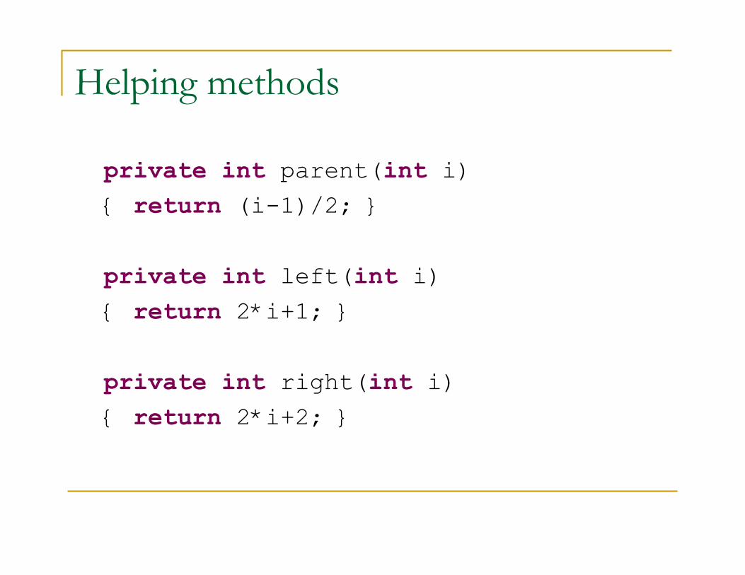
Helping methods
private int parent(int i)
{ return (i-1)/2; }
private int left(int i)
{ return 2*i+1; }
private int right(int i)
{ return 2*i+2; }
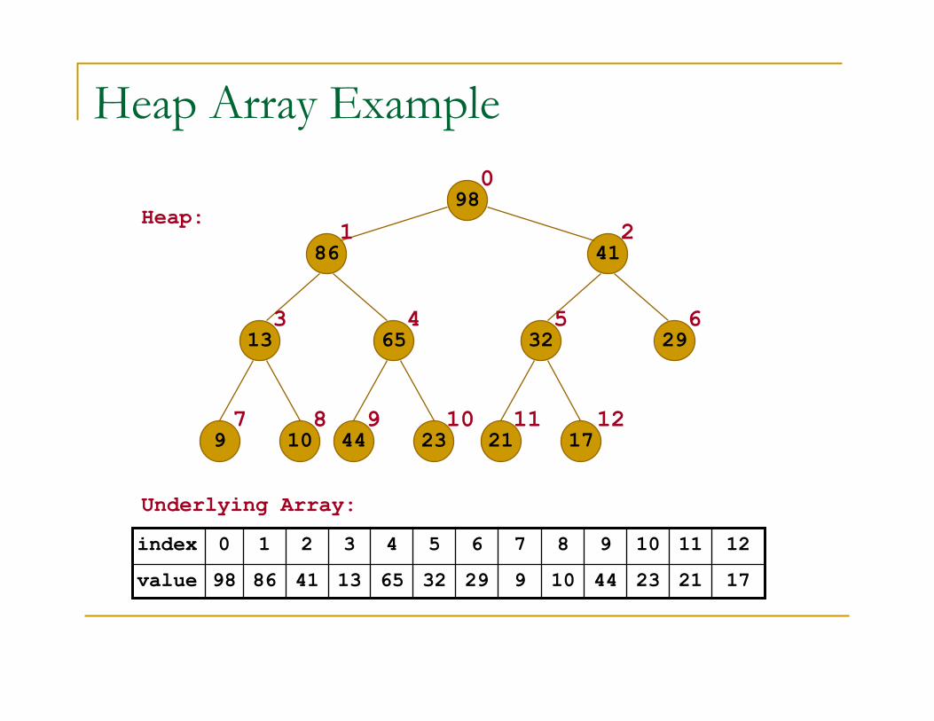
Heap Array Example
98
4186
13 65
9 10
32 29
44 23 21 17
17
12
21234410929326513418698value
11109876543210index
Heap:
Underlying Array:
0
1 2
3 54 6
7 8 9 10 11 12
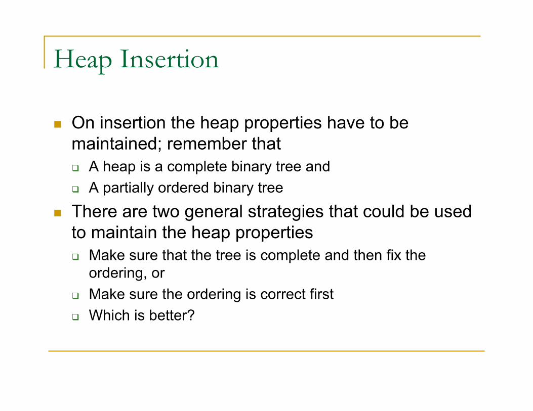
Heap Insertion
� On insertion the heap properties have to be
maintained; remember that
� A heap is a complete binary tree and
� A partially ordered binary tree
� There are two general strategies that could be used
to maintain the heap properties
� Make sure that the tree is complete and then fix the
ordering, or
� Make sure the ordering is correct first
� Which is better?
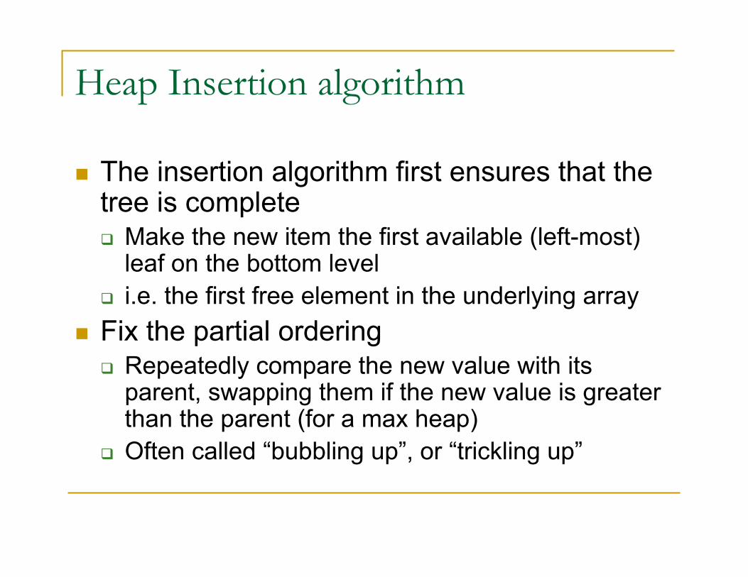
Heap Insertion algorithm
� The insertion algorithm first ensures that the tree is complete� Make the new item the first available (left-most) leaf on the bottom level
� i.e. the first free element in the underlying array
� Fix the partial ordering
� Repeatedly compare the new value with its parent, swapping them if the new value is greater than the parent (for a max heap)
� Often called “bubbling up”, or “trickling up”
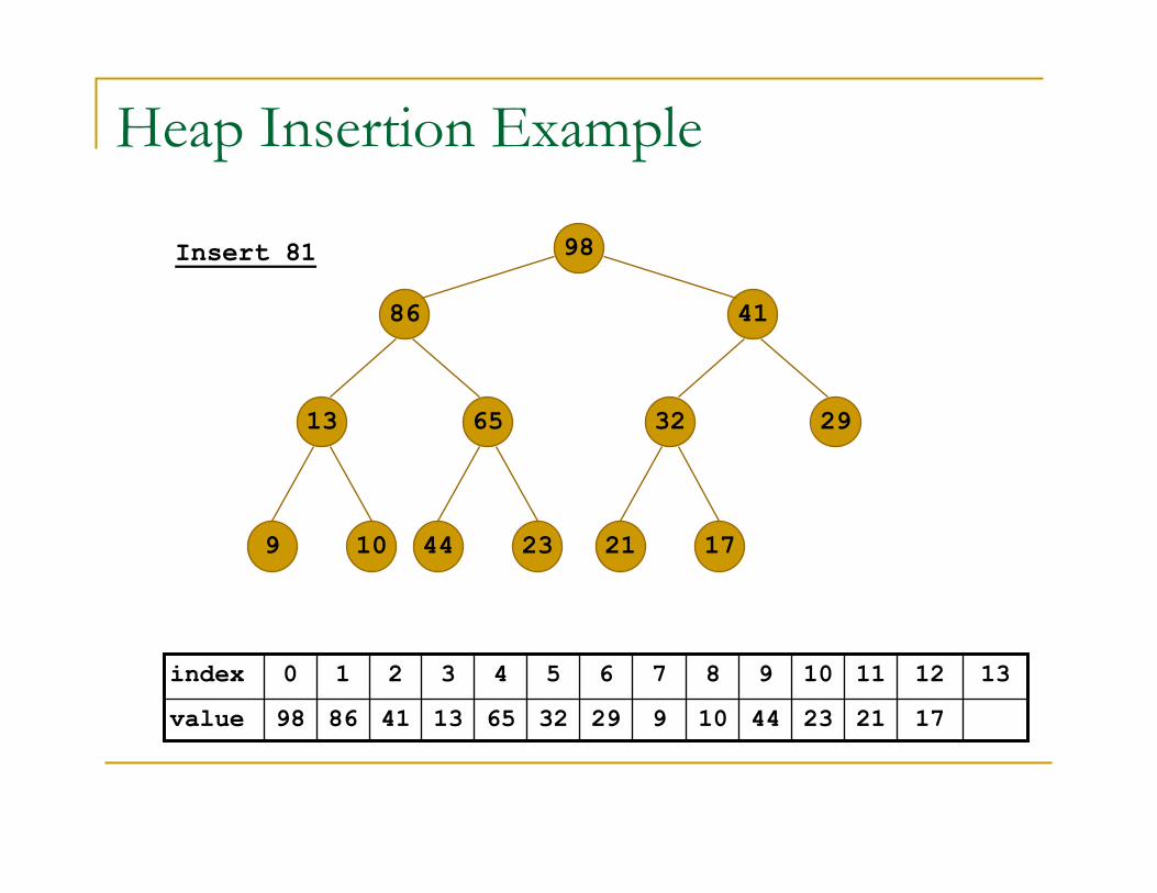
Heap Insertion Example
98
4186
13 65
9 10
32 29
44 23 21 17
17
12
81
13
21234410929326513418698value
11109876543210index
Insert 81
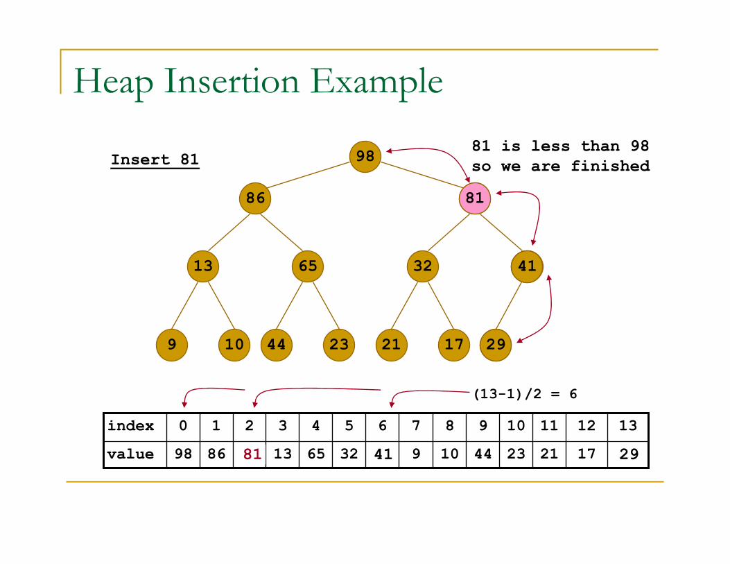
Heap Insertion Example
98
4186
13 65
9 10
32 29
44 23 21 17
17
12
81
13
21234410929326513418698value
11109876543210index
Insert 81
81
81
29
81
81
41
(13-1)/2 = 6
298141
81 is less than 98
so we are finished
Heap Insertion algorithm
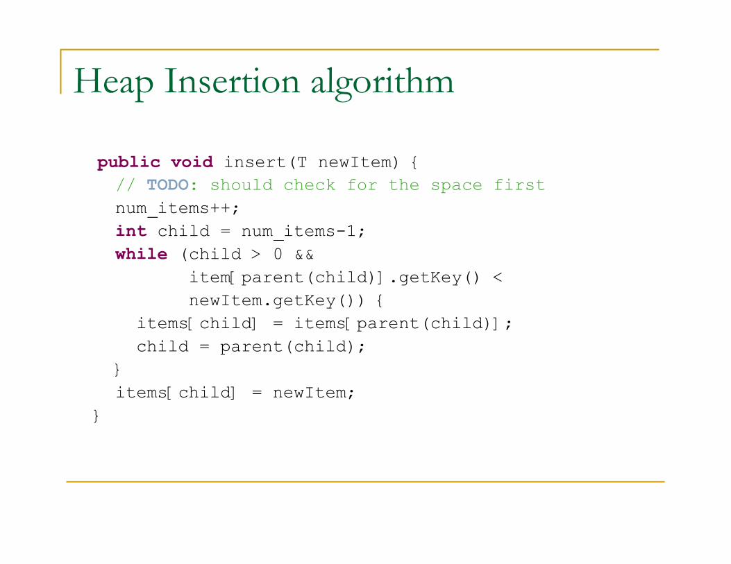
public void insert(T newItem) {
// TODO: should check for the space first
num_items++;
int child = num_items-1;
while (child > 0 &&
item[parent(child)].getKey() <
newItem.getKey()) {
items[child] = items[parent(child)];
child = parent(child);
}
items[child] = newItem;
}
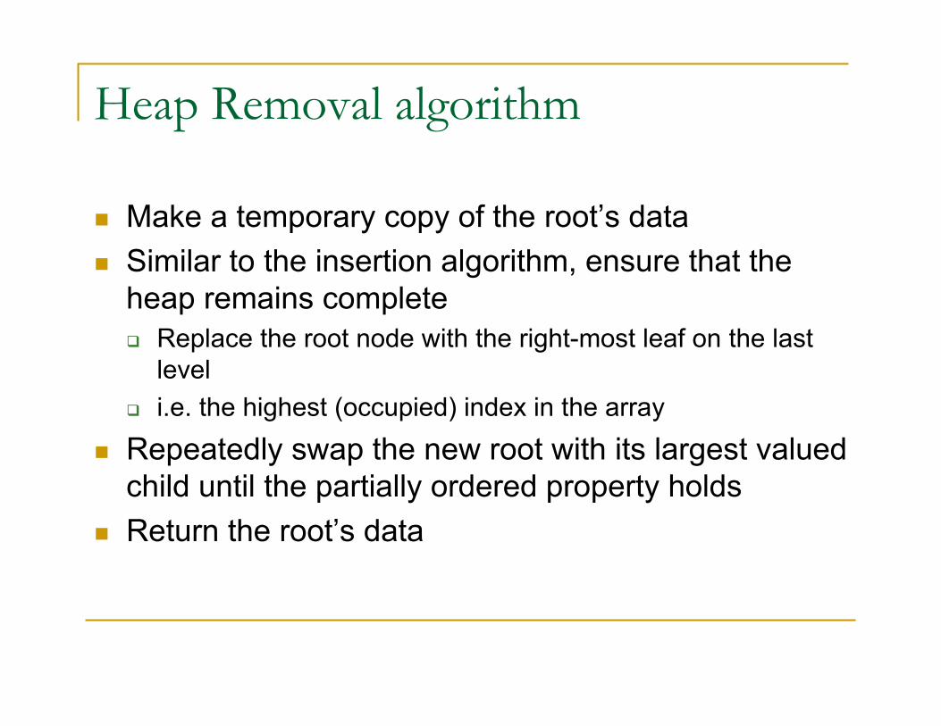
Heap Removal algorithm
� Make a temporary copy of the root’s data
� Similar to the insertion algorithm, ensure that the
heap remains complete
� Replace the root node with the right-most leaf on the last
level
� i.e. the highest (occupied) index in the array
� Repeatedly swap the new root with its largest valued
child until the partially ordered property holds
� Return the root’s data
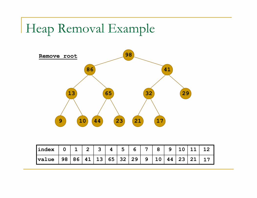
Heap Removal Example
98
4186
13 65
9 10
32 29
44 23 21 17
17
12
21234410929326513418698value
11109876543210index
Remove root
17
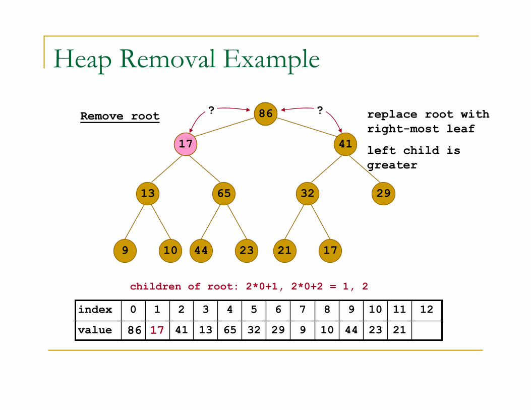
Heap Removal Example
98
4186
13 65
9 10
32 29
44 23 21 17
17
12
21234410929326513418698value
11109876543210index
Remove root
17
17
17
children of root: 2*0+1, 2*0+2 = 1, 2
17
86
86
left child is
greater
replace root with
right-most leaf
??
1765
86
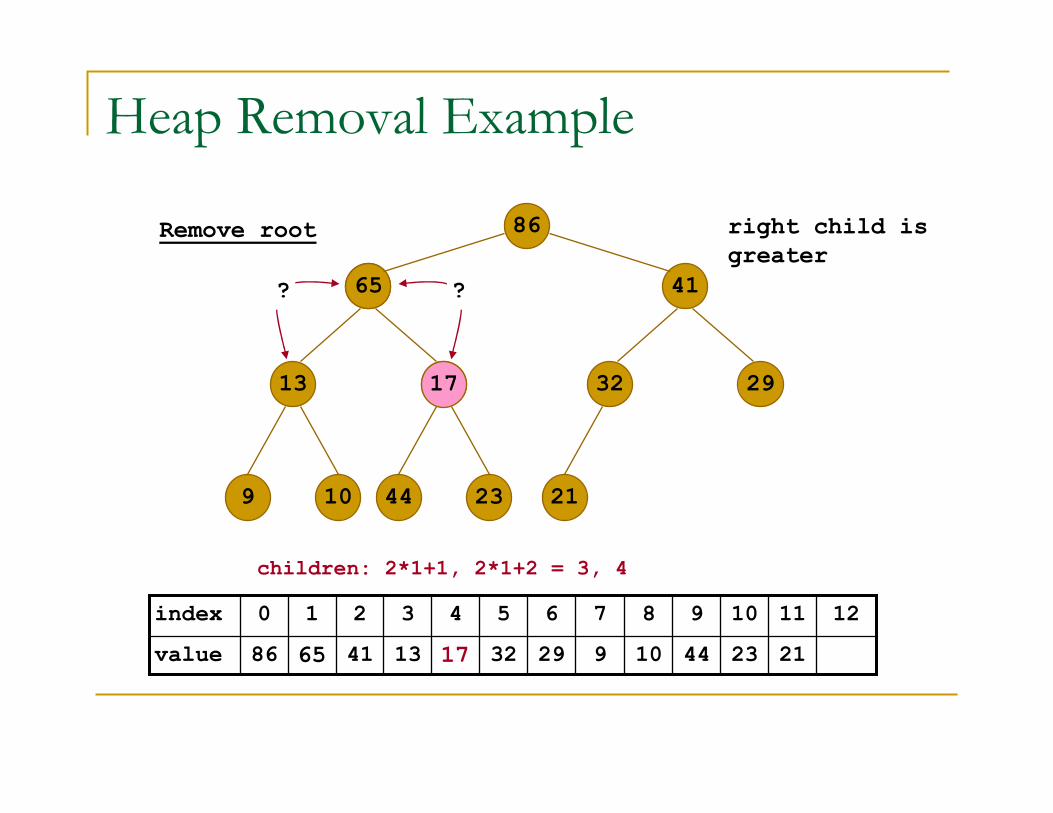
Heap Removal Example
41
13 65
9 10
32 29
44 23 21
12
21234410929326513418686value
11109876543210index
Remove root
17
17
1765
children: 2*1+1, 2*1+2 = 3, 4
right child is
greater
? ?
1744
12
21234410929321713416586value
11109876543210index
1744
65
86
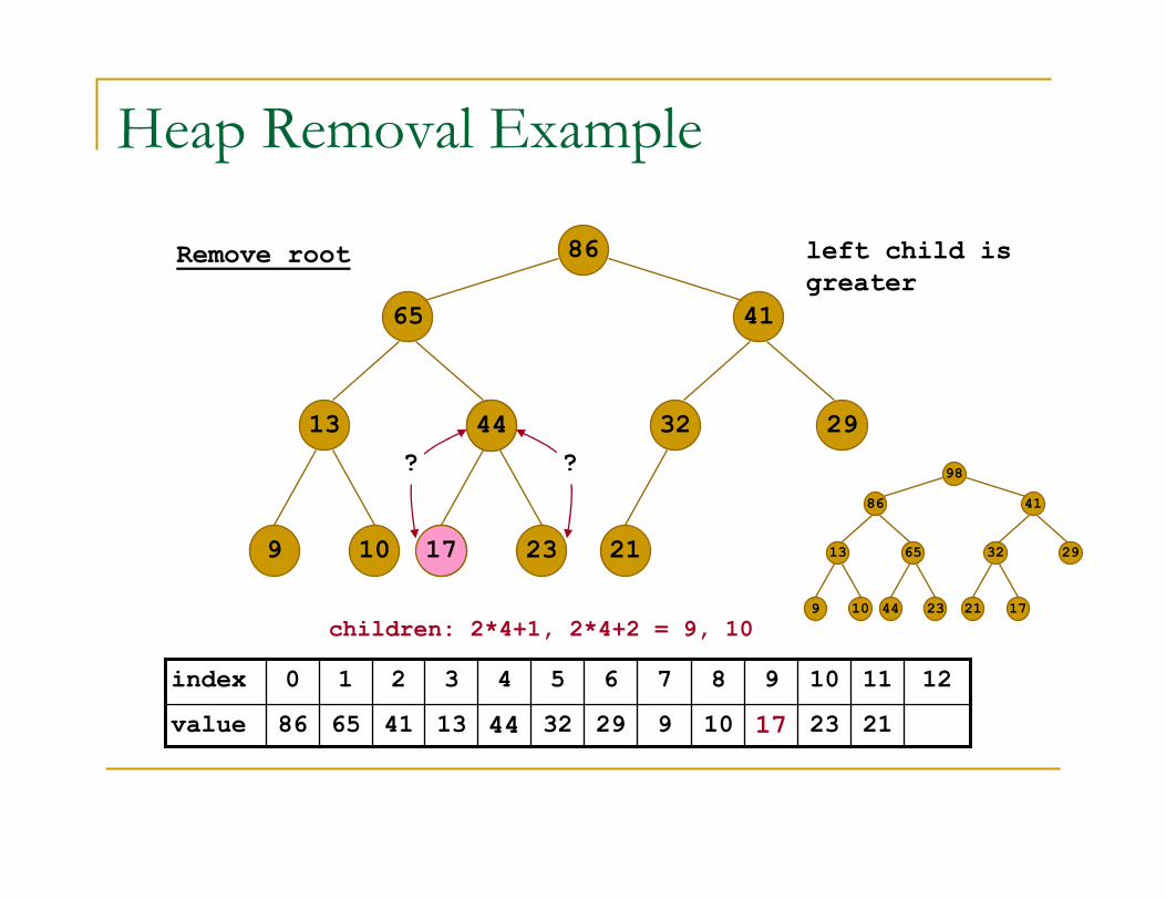
Heap Removal Example
41
13
9 10
32 29
44 23 21
Remove root
17
children: 2*4+1, 2*4+2 = 9, 10
left child is
greater
??98
4186
13 65
9 10
32 29
44 23 21 17
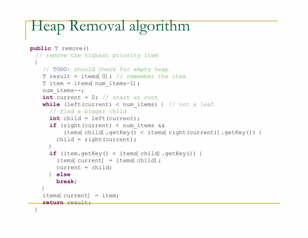
Heap Removal algorithm
public T remove()
// remove the highest priority item
{
// TODO: should check for empty heap
T result = items[0]; // remember the item
T item = items[num_items-1];
num_items--;
int current = 0; // start at root
while (left(current) < num_items) { // not a leaf
// find a bigger child
int child = left(current);
if (right(current) < num_items &&
items[child].getKey() < items[right(current)].getKey()) {
child = right(current);
}
if (item.getKey() < items[child].getKey()) {
items[current] = items[child];
current = child;
} else
break;
}
items[current] = item;
return result;
}
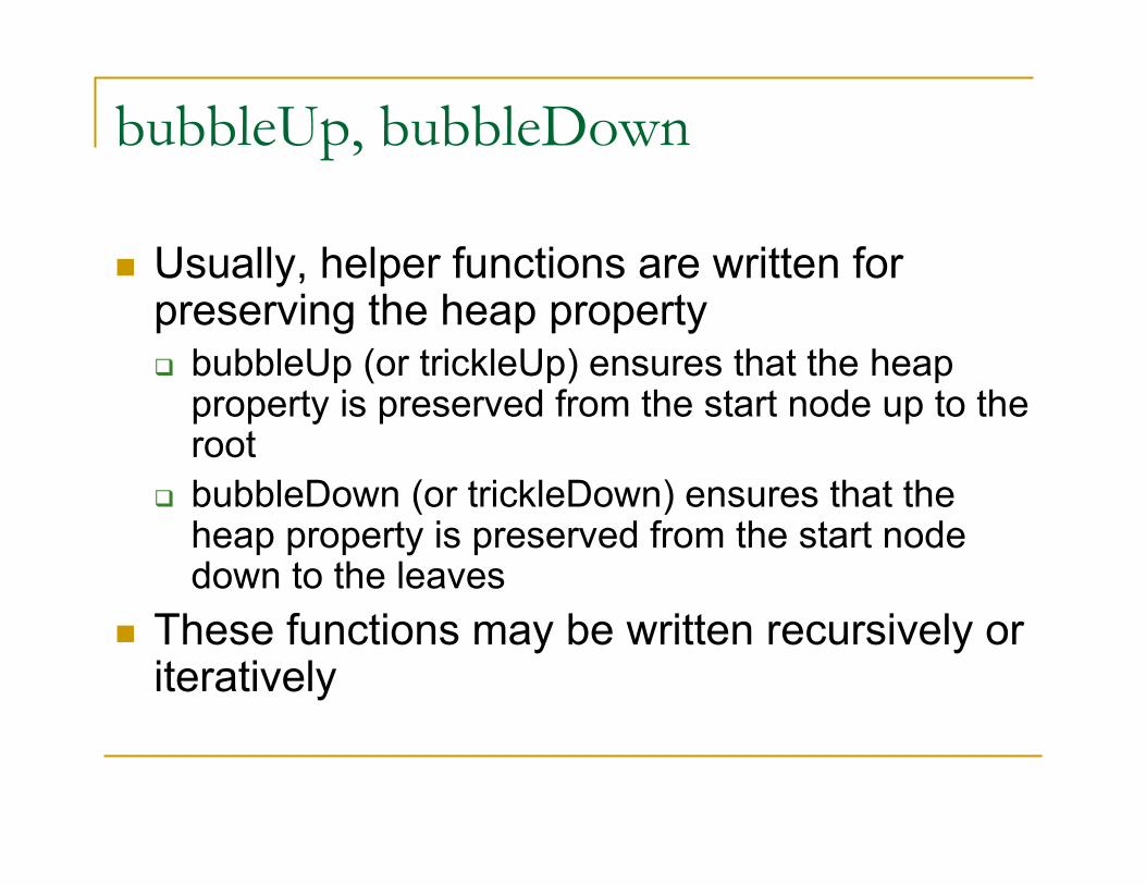
bubbleUp, bubbleDown
� Usually, helper functions are written for preserving the heap property� bubbleUp (or trickleUp) ensures that the heap property is preserved from the start node up to the root
� bubbleDown (or trickleDown) ensures that the heap property is preserved from the start node down to the leaves
� These functions may be written recursively or iteratively
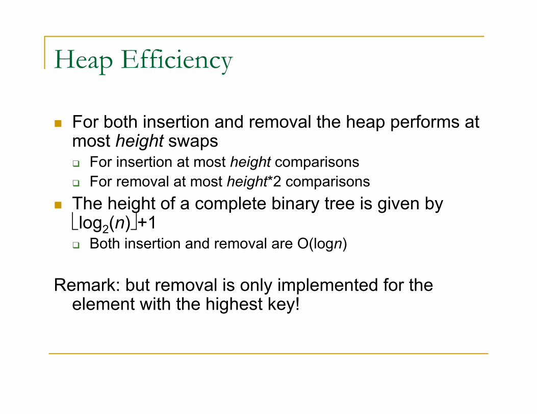
Heap Efficiency
� For both insertion and removal the heap performs at most height swaps� For insertion at most height comparisons
� For removal at most height*2 comparisons
� The height of a complete binary tree is given by log2(n)+1� Both insertion and removal are O(logn)
Remark: but removal is only implemented for the element with the highest key!
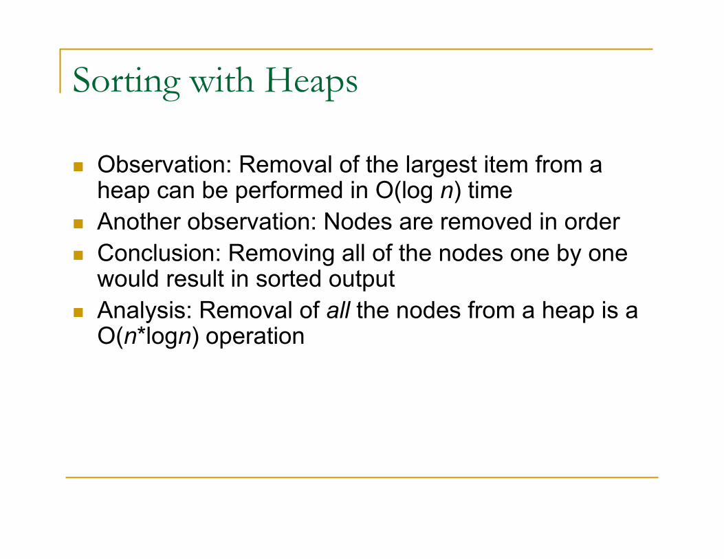
Sorting with Heaps
� Observation: Removal of the largest item from a heap can be performed in O(log n) time
� Another observation: Nodes are removed in order
� Conclusion: Removing all of the nodes one by one would result in sorted output
� Analysis: Removal of all the nodes from a heap is a O(n*logn) operation
But …
� A heap can be used to return sorted data� in O(n*log n) time
� However, we can’t assume that the data to be sorted just happens to be in a heap!
� Aha! But we can put it in a heap.
� Inserting an item into a heap is a O(log n) operation so inserting n items is O(n*log n)
� But we can do better than just repeatedly calling the insertion algorithm
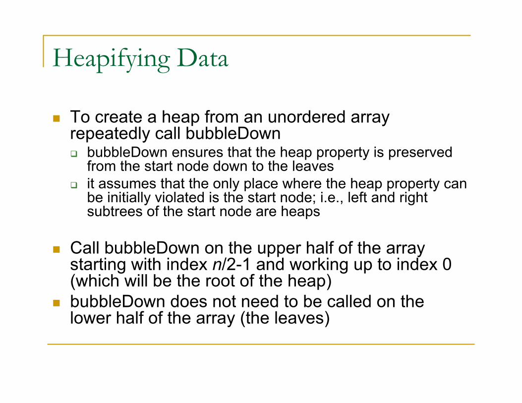
Heapifying Data
� To create a heap from an unordered array repeatedly call bubbleDown� bubbleDown ensures that the heap property is preserved
from the start node down to the leaves
� it assumes that the only place where the heap property can be initially violated is the start node; i.e., left and right subtrees of the start node are heaps
� Call bubbleDown on the upper half of the array starting with index n/2-1 and working up to index 0 (which will be the root of the heap)
� bubbleDown does not need to be called on the lower half of the array (the leaves)
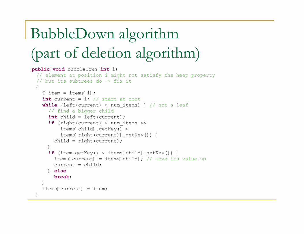
BubbleDown algorithm
(part of deletion algorithm)public void bubbleDown(int i)
// element at position i might not satisfy the heap property
// but its subtrees do -> fix it
{
T item = items[i];
int current = i; // start at root
while (left(current) < num_items) { // not a leaf
// find a bigger child
int child = left(current);
if (right(current) < num_items &&
items[child].getKey() <
items[right(current)].getKey()) {
child = right(current);
}
if (item.getKey() < items[child].getKey()) {
items[current] = items[child]; // move its value up
current = child;
} else
break;
}
items[current] = item;
}
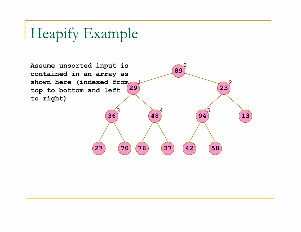
Heapify Example
89
2329
36 48
27 70
94 13
76 37 42 58
Assume unsorted input is
contained in an array as
shown here (indexed from
top to bottom and left
to right)
0
1 2
3 54
58
9423 13
27 37 4270 76
Heapify Example
89
2329
36 48
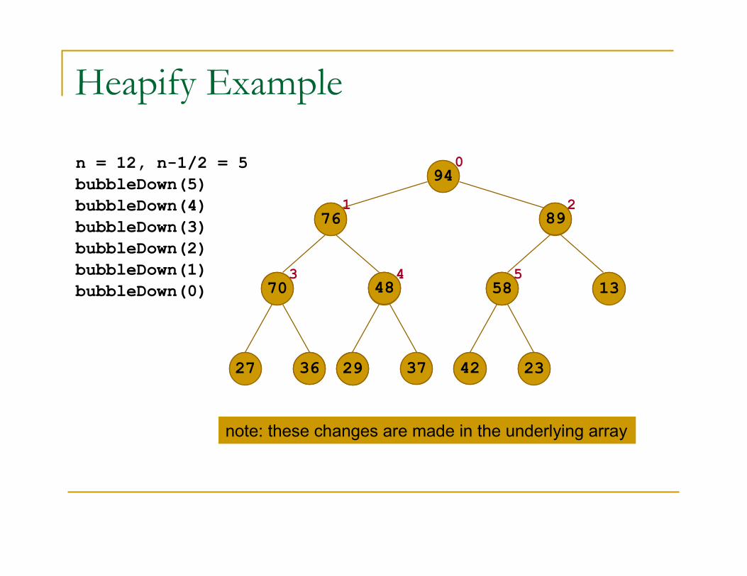
n = 12, n-1/2 = 5
bubbleDown(5)
bubbleDown(4)
bubbleDown(3)
bubbleDown(2)
bubbleDown(1)
bubbleDown(0)
940
1 2
3 54
note: these changes are made in the underlying array
48
7670
36 23
58
9476
29
29
48
36 29
70
76
27 37
48
23
13
89
58
42
Heapify algorithm
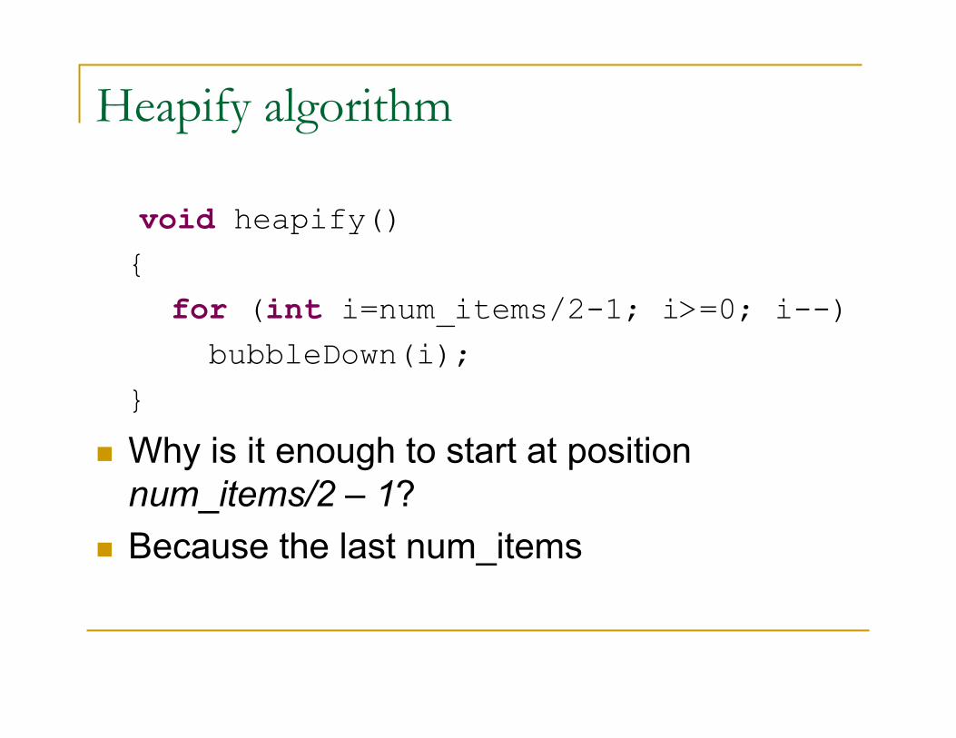
void heapify()
{
for (int i=num_items/2-1; i>=0; i--)
bubbleDown(i);
}
� Why is it enough to start at position
num_items/2 – 1?
� Because the last num_items
Cost to Heapify an Array
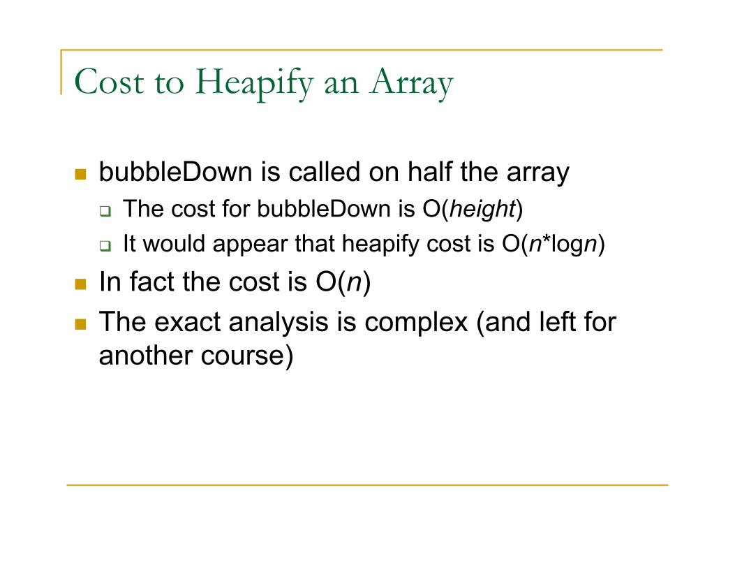
� bubbleDown is called on half the array
� The cost for bubbleDown is O(height)
� It would appear that heapify cost is O(n*logn)
� In fact the cost is O(n)
� The exact analysis is complex (and left for
another course)
HeapSort Algorithm Sketch
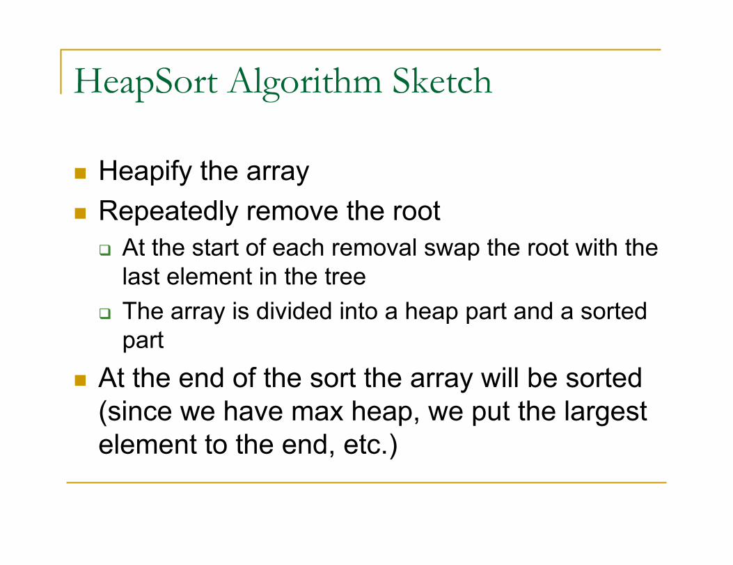
� Heapify the array
� Repeatedly remove the root
� At the start of each removal swap the root with the
last element in the tree
� The array is divided into a heap part and a sorted
part
� At the end of the sort the array will be sorted
(since we have max heap, we put the largest
element to the end, etc.)
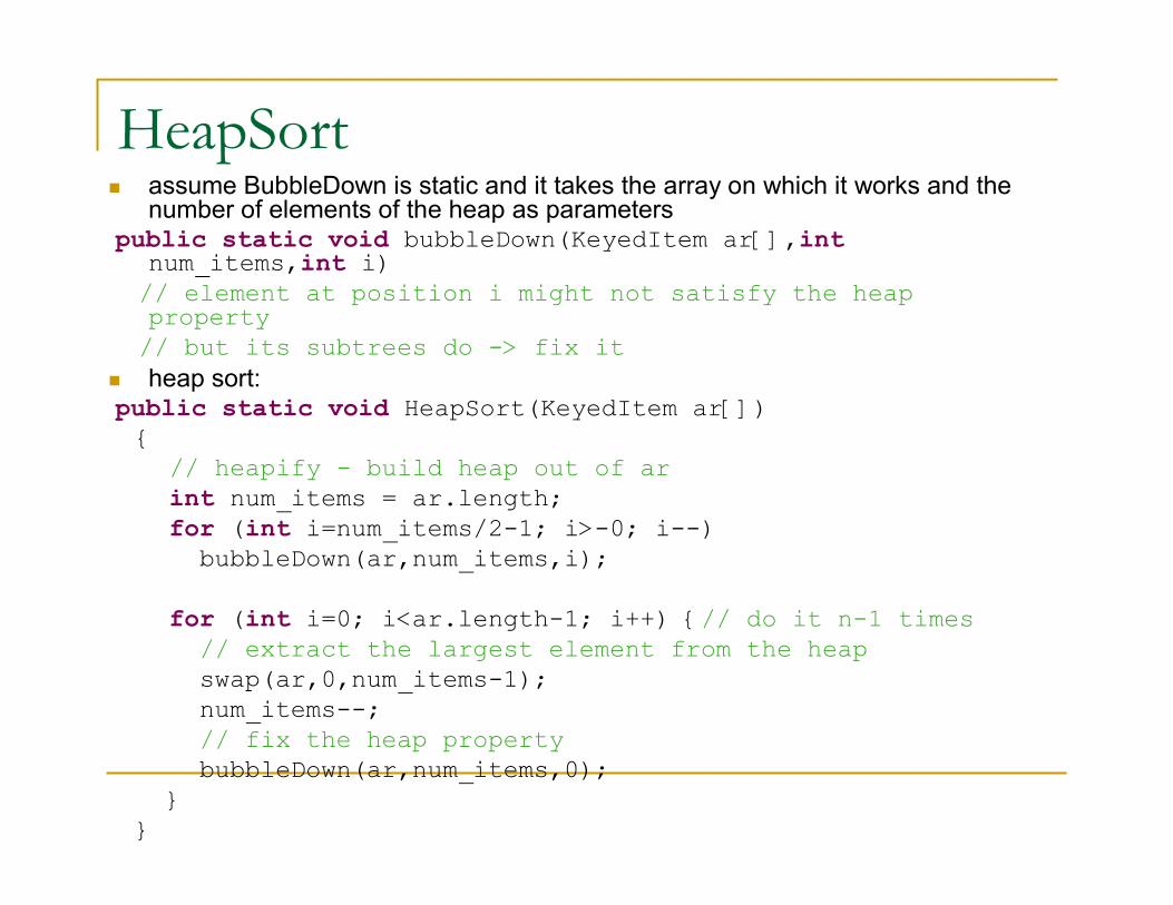
HeapSort� assume BubbleDown is static and it takes the array on which it works and the
number of elements of the heap as parameterspublic static void bubbleDown(KeyedItem ar[],int
num_items,int i)
// element at position i might not satisfy the heap property
// but its subtrees do -> fix it
� heap sort:public static void HeapSort(KeyedItem ar[]){
// heapify - build heap out of ar
int num_items = ar.length;
for (int i=num_items/2-1; i>-0; i--)
bubbleDown(ar,num_items,i);
for (int i=0; i<ar.length-1; i++) {// do it n-1 times
// extract the largest element from the heap
swap(ar,0,num_items-1);
num_items--;
// fix the heap property
bubbleDown(ar,num_items,0);
}
}
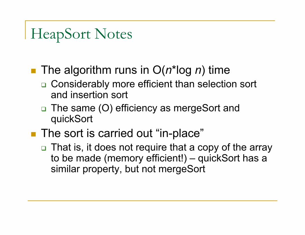
HeapSort Notes
� The algorithm runs in O(n*log n) time� Considerably more efficient than selection sort and insertion sort
� The same (O) efficiency as mergeSort and quickSort
� The sort is carried out “in-place”� That is, it does not require that a copy of the array to be made (memory efficient!) – quickSort has a similar property, but not mergeSort