
Table of Contents - hp.com · HP Prime AP Calculus Summer Institute Materials by Mark Howell...
75
Transcript of Table of Contents - hp.com · HP Prime AP Calculus Summer Institute Materials by Mark Howell...

HP Prime AP Calculus Summer Institute Materials by Mark Howell Version 1.3
HP Prime AP Calculus Summer Institute Last Revised May 25, 2016 Page 2 of 75
Table of Contents
Introduction to HP Prime 3-6
Getting Started: The Function App 7-9
Limits, Asymptotes, and Zooming 10-15
Introducing the Derivative 16-19
AP Free Response Style Question #1 20-23
Sunrise-Sunset Data Activity (Precalculus) 24-29
Sunrise-Sunset Data Activity (Calculus) 30-35
The Derivative Function 36-39
Implicit Differentiation 40-44
Approximating Integrals with Riemann Sums 45-52
Fundamental Theorem Investigation 53-62
Differential Equations and Slopefields 63-69
AP Free Response Style Question #2 70-72
Primed for the AP Calculus Exam 73-75

HP Prime AP Calculus Summer Institute Materials by Mark Howell Version 1.3
© 2015 by HP Calculators Last Revised May 25, 2016 Page 3 of 75
Introduction to HP Prime
HP Prime is a color, touchscreen graphing calculator, with multi-touch capability, a Computer
Algebra System (CAS), an Advanced Graphing app that lets you graph any relation in two variables
(graphing something like sin cosxy xy for example), and a dynamic geometry app. In this
section, we'll take a look at how to find your way around HP Prime, and get acquainted with the Function app.
First, here are a few conventions we'll use in this document:
A key that initiates an unshifted function is represented by an image of that key: $, H, j and so on.
A key combination that initiates a shifted function (or inserts a character) is represented by the appropriate shift key (S or A) followed by the key for that function or character: Sj initiates the natural exponential function and Af inserts the letter F.
The name of the shifted function may also be given in parentheses after the key
combination: S& (Clear), S# (Plot Setup)
A key pressed to insert a digit is represented by that digit: 5, 7, 8, and so on.
All fixed on-screen text—such as screen and field names—appear in bold: CAS Settings, Xstep, Decimal Mark, and so on.
A menu item selected by touching the screen is represented by an image of that item:
, , , and so on.
NOTE: You must use your finger to select a menu item, or navigate to the selection and press E.
Cursor keys are represented by D, L , R , and U. You use these keys to move from field
to field on a screen, or from one option to another in a list of options.
The ON-OFF key is at the bottom left of the keyboard. When a new HP Prime is turned on for the first
time, a "splash" screen appears that invites the user to select a language and to make some initial setup choices. For most users, accepting the default options is the way to go.
The screen brightness can be increased by pressing and holding Oand ;or decreased by
pressing and holding O and -.
Take a minute to look at the layout of the keyboard. The top group of keys, with the black background, are primarily for navigating from one environment to another. Pressing H takes you
to the home calculation screen, and pressing C takes you to a similar calculation environment for doing symbolic or exact computations. Pressing ! takes you to a menu where you can select from
all the applications in the HP Prime, like Function or Parametric or Geometry. The bottom group of

HP Prime AP Calculus Summer Institute Materials by Mark Howell Version 1.3
© 2015 by HP Calculators Last Revised May 25, 2016 Page 4 of 75
keys is mainly for entering or editing mathematical expressions. There are also environments for entering lists, S 7 , matrices, S4, and user programs, S1.
Some care was taken when deciding where to place certain keys. The number for instance, is
S3. The list delimiters, {}, appear just to the right of the LIST key, S8and the matrix
delimiters, [], appear just to the right of the MATRIX key, S5.
Things you can do in both CAS and Home views:
Tap an item to select it or tap twice to copy it to the command line editor
Tap and drag up or down to scroll through the history of calculations
Press M to retrieve a previous entry or result from the other view
Press the Toolbox key (b) to see the Math and CAS menus as well as the Catalog
Press c to open a menu of easy-to-use templates
Press & to exit these menus without making a selection
Tap , , and menu buttons once to activate
Home View
Turn on your HP Prime and take a look at the different sections of the screen in the HOME view.
The top banner across the top is called the Title Bar, and it tells you what operating environment you are currently working in (like HOME or FUNCTION
SYMBOLIC VIEW). If you press a shift key, an
annunciator comes on at the left of the Title Bar. On the right, you see a battery level indicator, a clock,
and the current angle mode. You can tap this Quick Settings section at the top right to see a calendar (by tapping the date and time), connect to a wireless classroom network (by tapping the wireless icon), or change the angle mode (by tapping the angle mode indicator).
The middle section of the HOME view contains a history of past calculations. You can navigate
through the history with the cursor keys, or using your finger to select (by tapping) or scroll (by swiping). The edit line is just below the history section. This is where you enter mathematical expressions to evaluate numerically. At the bottom
are the menu keys, consisting of in the HOME view. These menu keys are context sensitive.
Their labels and function changes depending on what environment you're in.
Home view is for numerical calculations, as the next few examples show. First, store 0 in the real variable X by entering 0 X. To enter the variable X, press S * (or d).
HP Prime AP Calculus Summer Institute Materials by Mark Howell Version 1.3
© 2015 by HP Calculators Last Revised May 25, 2016 Page 5 of 75
With 0 stored in X, press c and choose the derivative template. In the numerator, enter g A
*; then tap on the denominator and enter A *. Press E to see the result: the value of
the derivative of sin(X) (which is cos(X)), when X=0 is 1. For another example, enter 3+, then return to the Template menu and select the integral template. Let the integrand be LN(3*T) and the limits of integration be from 0 to X, as shown in the figure. Press E to see the result, which can be
seen by inspection to be 3, since X=0. The figure to the right also shows a summation. In all of these cases, the results evaluate to a real number. In Home view, all results evaluate to a real or a complex number, or a matrix, list, etc. of real and/or complex numbers. You can tap on any previous input or result in the history to select it. When you do, two new menu buttons appear: and . The former copies the selection to the cursor position while the later typesets the selection in textbook format in full-screen mode.
CAS View
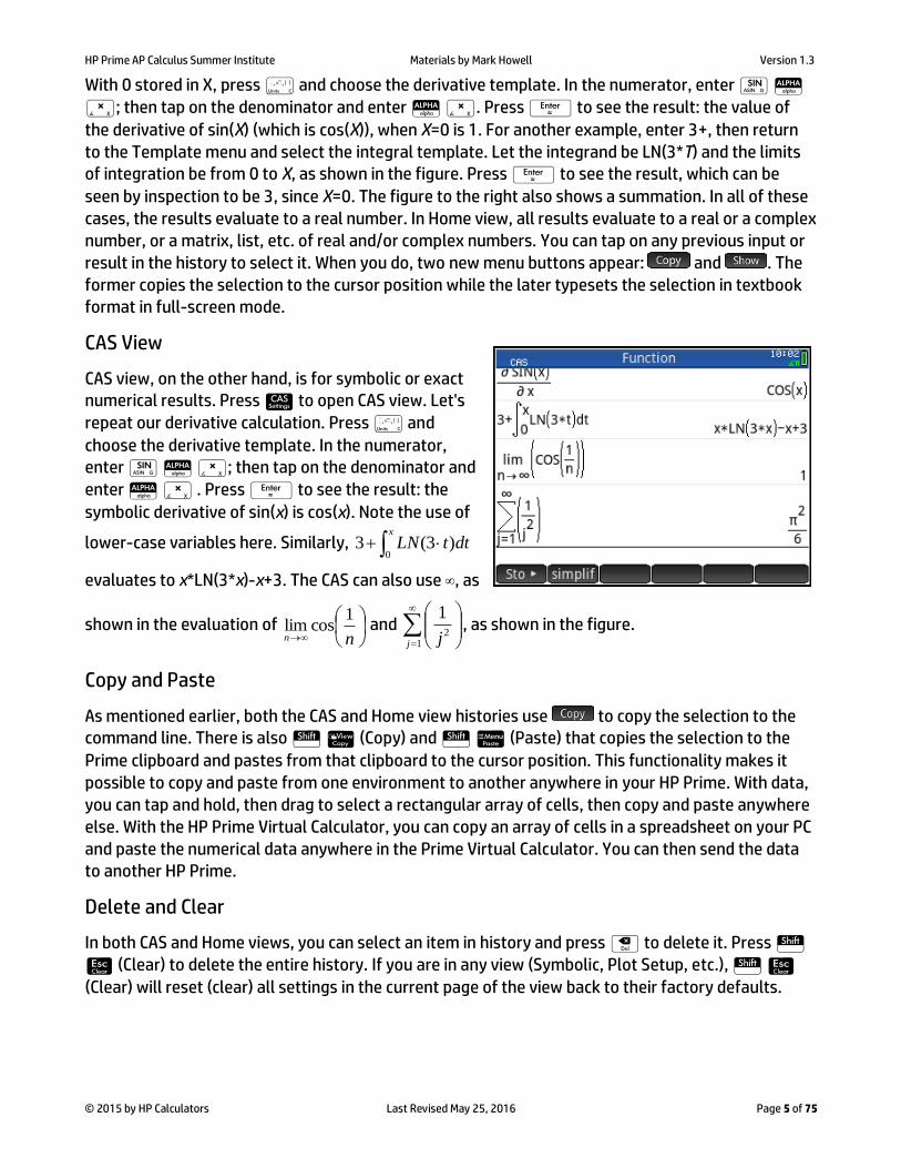
CAS view, on the other hand, is for symbolic or exact numerical results. Press C to open CAS view. Let's
repeat our derivative calculation. Press c and
choose the derivative template. In the numerator, enter g A *; then tap on the denominator and
enter A * . Press E to see the result: the
symbolic derivative of sin(x) is cos(x). Note the use of
lower-case variables here. Similarly, x
dttLN0
)3(3
evaluates to x*LN(3*x)-x+3. The CAS can also use ∞, as
shown in the evaluation of
nn
1coslim and
12
1
j j, as shown in the figure.
Copy and Paste
As mentioned earlier, both the CAS and Home view histories use to copy the selection to the command line. There is also S V (Copy) and S M (Paste) that copies the selection to the
Prime clipboard and pastes from that clipboard to the cursor position. This functionality makes it possible to copy and paste from one environment to another anywhere in your HP Prime. With data, you can tap and hold, then drag to select a rectangular array of cells, then copy and paste anywhere else. With the HP Prime Virtual Calculator, you can copy an array of cells in a spreadsheet on your PC and paste the numerical data anywhere in the Prime Virtual Calculator. You can then send the data to another HP Prime.
Delete and Clear
In both CAS and Home views, you can select an item in history and press \ to delete it. Press S & (Clear) to delete the entire history. If you are in any view (Symbolic, Plot Setup, etc.), S &
(Clear) will reset (clear) all settings in the current page of the view back to their factory defaults.

HP Prime AP Calculus Summer Institute Materials by Mark Howell Version 1.3
© 2015 by HP Calculators Last Revised May 25, 2016 Page 6 of 75
HP Prime Apps and Their Views
The HP Prime graphing calculator comes pre-loaded with a number of apps. Each app was designed
to explore and area of mathematics or to solve problems of a specific type. Every Prime app is divided into one or more views. Most commonly, an app has a Symbolic view, a Plot (or Graphic) view, and a Numeric view. In this sense, the apps all have a common structure so they are easier to learn to use as a set of apps. The Prime app schema is shown in the figure below.
Press ! to open the App Library. Tap on an app to start it, or navigate the library using the cursor
pad and tap to launch the app.
Fill the app with data while you work, and save it with a name you’ll remember. Then reset the app and use it for something else. You can come back to your saved app anytime-even send it to your
colleagues! HP Apps have app functions as well as app variables; you can use them while in the app, or from the CAS view, Home view, or in programs.
HP Apps and their Views
Symbolic Graphic (Plot) Numeric

HP Prime AP Calculus Summer Institute Materials by Mark Howell Version 1.3
© 2015 by HP Calculators Last Revised May 25, 2016 Page 7 of 75
Getting Started: The Function App
Let g be the function defined by x
dttxg0
2cos)( for 21 x . On what interval(s) is g
decreasing?
1. Press ! to open the App Library
and select the Function app. The app opens in Symbolic view. Press c to open the template menu and
tap on the integral template. Fill out the template as shown in the figure
and tap .
2. Press P to see the graph. Use
your fingers to drag and pinch until the viewing window shows the domain indicated in the problem statement above. Use the figure to
the right as a guide. For x-values
between -1 and 2, there appears to be only one interval in which g(x) is decreasing. That interval is from the relative maximum near x=1.2 to the domain endpoint at x=2.
3. Tap near the maximum at x≈1.2 to move the cursor near the
extremum. Tap , then tap
and select Extremum. The
left endpoint of the decreasing interval is approximately 1.2533.
So g(x) is decreasing on the interval
22533.1 x .

HP Prime AP Calculus Summer Institute Materials by Mark Howell Version 1.3
© 2015 by HP Calculators Last Revised May 25, 2016 Page 8 of 75
Two particles start at the origin and move along the x-axis. For 0≤t≤10, their respective
positions are given by )cos(1 tx and 122
x
ex . For how many values of t do the particles
have the same velocity? Here we use an indirect method to illustrate a useful technique.
1. Press C to open CAS view. Define
x1 and x2 as above.
Note: Prime uses := to define functions and variables.
Note: the mapping symbol (→) is supplied
by CAS after entry.
2. Press ! to open the App Library.
Navigate to the Function app and
tap .
3. Tap on the app to open it. The app opens in Symbolic view. We now define F1 and F2 to be the
derivatives, with respect to X, of x1 and x2. With the cursor on F1(X), press c to open the Template
menu and tap on the derivative template. In the numerator, enter
x1(X). In the denominator, enter X=X. Likewise, define F2(X) to be the derivative of x2(X) with respect to X.
Note: x1 and x2 use lowercase x, but the variable is uppercase X.
The notation X=X tells Prime that X here does not have a single value, as it does elsewhere in the system.
4. Press P to see the graphs. Again,
use your fingers to drag and pinch
to get the viewing window to match the domain stated in the problem. There are four points in time where the particles have the same
velocity.

HP Prime AP Calculus Summer Institute Materials by Mark Howell Version 1.3
© 2015 by HP Calculators Last Revised May 25, 2016 Page 9 of 75
We used this technique to illustrate that you can work in CAS as well as Plot view.
5. Press C to return to CAS view.
6. Press b to open the Toolbox menu.
Tap for the CAS menu and
select the Solve submenu. Tap on the solve command. Complete the command as shown in the figure.
Use the derivative template found by pressing c. The notation t=0..10 defines a domain
for t.
7. Press E to see the result.
Here the results were rounded to 4 places for readability. There are four values, which agrees with our Plot view investigation.

HP Prime AP Calculus Summer Institute Materials by Mark Howell Version 1.3
© 2015 by HP Calculators Last Revised May 25, 2016 Page 10 of 75
Limits, Asymptotes, and Zooming
HP Prime Functionality Introduced:
Using the Function App Symbolic, Plot, and Numeric views; zooming in to a graph; zooming in to a table
AP Calculus Content:
Limits at a point and at infinity; one-sided limits; horizontal and vertical asymptotes
Activity:
Press ! and select the Function App. Press
S& (Clear) and enter
2
21 2
1
xF x
x
, as
shown.
Here, you will investigate the behavior of this function in its graphic and numeric representations, as the values of x grow without bound.
First, press V and select 4 to see the graph in the
decimal view. In this view, pixels are 0.1 units horizontally and vertically. You should see the graph at right.
With HP Prime, it is a simple matter to look at the graphic behavior for large values of x. Simply swipe your finger horizontally from right to left on the graph to scroll to the right. Tap the graph after it appears to become horizontal, and the input and output will be displayed at the input where you tap. Enter the values of X and F1(X) you see.
1. X___________________________ F1(X) ________________________
Swipe your finger a few more times in the same manner and again record the values of X and F1(X)
2. X___________________________ F1(X) ________________________
3. You should see that the values of F1(X) are pretty close to a positive integer. What is that integer? ___________________

HP Prime AP Calculus Summer Institute Materials by Mark Howell Version 1.3
© 2015 by HP Calculators Last Revised May 25, 2016 Page 11 of 75
Now let's look at this behavior numerically in a table of values.
Press N to see a table of inputs and outputs for F1.
There are several ways to look at the outputs from F1(X) for large values of X. One is to simply enter a value for X. With the cursor anywhere in the column for X, enter 10. The table immediately adjusts to the new value.
Enter 100, then 1000, then 1000000 for X, and observe each time what happens to the outputs from F1(X). You should see them approaching the same integer you gave as your answer to question 3.
In mathematical language, we say that the limit of F1(X) as x approaches positive infinity is 3, and express that result with this notation:
lim 1 3x
F x
.
We also say that the line 3y is a horizontal asymptote for the graph of
2
22
1
xy
x
. Notice
that we can make the values of F1(X) as close as we want to 3 (within the limitations of the numerical precision of the calculator) by making the inputs, X, sufficiently large. You can also use a horizontal pinch to zoom horizontally. Place two fingers together horizontally in Plot view, pause a moment, and then move them apart horizontally to zoom in on just the x-values.
You will see a pair of blue horizontal arrows indicating that horizontal zoom is active.
Let's take a look at using HP Prime to investigate the behavior of the outputs from F1(X) for values of X close to -1. Press V and select 4 to restore the
decimal view. Then simply press m1 to move the
cursor to a point with an x-coordinate of -1. This time, we'll use the Split Screen: Plot-Table View to
explore the function's behavior. With the cursor on a point with x-coordinate -1, press V 2 to select the Split Screen: Plot-Table view.

HP Prime AP Calculus Summer Institute Materials by Mark Howell Version 1.3
© 2015 by HP Calculators Last Revised May 25, 2016 Page 12 of 75
4. The output for x = -1 appears as NaN (calculator-speak for "not-a-number"). Why is there no
output at x = -1? ________________________________________________________________
______________________________________________________________________________
Press , and select 5 Xin. This changes the horizontal scale only, leaving the vertical scale
unchanged. Notice that the values in the table adjust as you zoom in. Press , and select 5 Xin
several more times. If necessary, swipe vertically on the graph to keep it in view. You can also use the horizontal pinch gesture described above to zoom in. What appears to be happening with the function outputs as the inputs get close to -1? What is happening with the graph?
______________________________________________________________________________
______________________________________________________________________________ ______________________________________________________________________________
You can also zoom in vertically using a pinch gesture. Place two fingers vertically in Plot view, pause
a moment, and move them apart to zoom in. You will see two vertical blue arrows indicating that a vertical zoom is active.
Here, we say that
)(1lim1
xFx
. (We might also say that the function has no limit as x
approaches -1.) The values of the function increase without bound as the inputs approach -1. We
also say that the line 1x is a vertical asymptote for the graph of
2
22
1
xy
x
.
From this example, the idea of limit might seem simple enough. But it can be quite slippery, as the next example illustrates. Press @, and tap the
check mark to the left of F1(X) to deselect it. Then
enter sin
2 1x
F xx
. Again, press V and
select 4 to see the graph in the decimal view. You should see the graph at right. Proceed as you did
for the previous example, and scroll to the right to see what happens to the values of F2(X) as x gets large.
5. What is sin
lim 1x
x
x
? ___________________

HP Prime AP Calculus Summer Institute Materials by Mark Howell Version 1.3
© 2015 by HP Calculators Last Revised May 25, 2016 Page 13 of 75
After you have scrolled to the right and the graph appears to be horizontal, tap on the graph, press
the key and then press , and select 7 Yin. You can also use a vertical pinch gesture.
Place two fingers vertically in Plot view and move them apart vertically.
This leaves the horizontal scale unchanged, but zooms in vertically. Zoom in vertically several
times, until you can see that the graph is not really horizontal at all! Zoom out ( 4 Out) a few
times to get a better idea of what's going on. You should see that the amplitude of the oscillations is getting smaller as the value of x get larger. This example illustrates why, even though
sinlim 1 1x
x
x
, we can't say that the values of
the function are "getting closer and closer to 1". It is
more appropriate to say something like, "We can
make the values of sin
1x
x as close as we want to
1 by making the values of x sufficiently large."
Press Nand enter 0 into any cell in the X column. We can zoom in to the table in the same way we
zoomed into a graph. With 0 selected in the X column, press and select 1 In. Notice that the
step size changes in the table. Press +, a shortcut for zooming in, several times. Of course, you
can also use a vertical pinch gesture to zoom in or out on a row in the table.
6. What is
0
sinlim 1x
x
x
? _______________________

HP Prime AP Calculus Summer Institute Materials by Mark Howell Version 1.3
© 2015 by HP Calculators Last Revised May 25, 2016 Page 14 of 75
Extension:
An HP Prime App called "Limits" contains definitions for these, and other, functions. Collectively,
these examples illustrate just about every type of limit problem you might encounter. Distribute the Limits App to students. Then have them investigate each function at the indicated point, and make a conclusion for each using the language of limits.
2 4
32
xF x
x
; x = 2
1
4 sinF xx
; x = 0
1
5 sinF x xx
; x = 0
1
6 arctanF xx
; x = 0; Use the language of one-sided limits
2
1 17 arctanF x
x
; x = 0
2
82
xF x
x
; x = 2; Use the language of one-sided limits
2
, if 29 4
4 ,if 2
xx
F x
x x
; x = 2; Use the language of one-sided limits
Note: you can add a third branch to a piecewise-defined function. Place the cursor at the end of the second branch and press o.
22 3
02 5 3
x x
x xF x
; x and x ; Also describe the horizontal and vertical asymptotes

HP Prime AP Calculus Summer Institute Materials by Mark Howell Version 1.3
© 2015 by HP Calculators Last Revised May 25, 2016 Page 15 of 75
Answers
1. Answers will vary. X = 61, F1(X) = 2.968
2. Answers will vary. X = 146, F1(X) = 2.98644
3. 3
4. Trying to evaluate F1(1) results in division by 0
5. The graph is becoming close to vertical.
6. 1
7. 2

HP Prime AP Calculus Summer Institute Materials by Mark Howell Version 1.3
© 2015 by HP Calculators Last Revised May 25, 2016 Page 16 of 75
Introducing the Derivative
HP Prime Functionality Introduced:
Drawing a tangent line to the graph of a function; using STO> to store the X and Y coordinates of the trace cursor on the graph into variables; evaluating a difference quotient on the HOME screen
AP Calculus Content:
Local linearity; differentiability; limit of an average rate of change to get the slope of a curve at a point; introduction of the derivative at a point
Activity:
Press ! and select the Function App. Press S& (Clear), and enter 1 sinF x x . Press V
and select 4 Decimal to see the graph in the decimal view. Press +, a shortcut for zooming in,
several times, until the graph keeps the same shape.
1. What happened to the shape of the graph as you zoomed in?
____________________________________________________________________________
Make sure the cursor is on the point where X = 0. Press , and then press . Select 5 Tangent to draw the tangent line to the graph of F1 at X = 0.
2. What appears to be true about the graph of 1 sinF x x and its tangent line at X = 0?
____________________________________________________________________________
Press -a few times until you can see a difference between the tangent line and the graph of
1 sinF x x . It appears that an equation for the tangent line is y = x. We could use the y-
coordinate of a point on the tangent line to approximate the y-coordinate of a point on the graph of
1 sinF x x .
3. When x = 0.2, what is the y-coordinate on the tangent line? ___________________________
Press , then enter 0.2 to move the cursor to the point on the graph of 1 sinF x x where
x = 0.2.
4. What is sin 0.2 ? ___________________________ How big is the error if we used the
tangent line to approximate sin 0.2 ? ________________________________ (The answer
comes from subtracting you answer to the first part of question 4 from your answer to question 3.)

HP Prime AP Calculus Summer Institute Materials by Mark Howell Version 1.3
© 2015 by HP Calculators Last Revised May 25, 2016 Page 17 of 75
Press V and select 4 to see the graph in the
decimal view. Press H. Now you will store the
cursor coordinates, which HP Prime keeps internally in the variables X and Y, into the variables A and B.
Enter X A A E,and Y A B E to do this. Press P, then press R to move
the cursor one pixel to the right of X = 0. Press H,
and enter the expression AX
BY
.
This expression, AX
BY
, is called a difference quotient (it is the quotient of two differences), and
represents the slope of the line segment joining the points ,sinX X and ,sinA A . It also
represents the average rate of change of 1 sinF x x on the closed interval [ , ]A X . In this case,
A = 0.
Now you will zoom in to the graph and recalculate this average rate of change. Press P, then
press L to move the cursor back to the point where X = 0. Press + one time to zoom in, then
press R to move the cursor one pixel to the right of X = 0. Press H. Now, all you have to do is
press Eto reevaluate the difference quotient with the new point. Repeat this process several
times: go back to the graph, move the cursor to X=0, zoom in, move the cursor one pixel to the right of X=0, go HOME, and recalculate the difference quotient. You should observe two important and
related things going on: the graph straightening out, and the difference quotients converging to a limit.
Now, press V and select 4 to get back to the decimal view. Press L several times to move the
cursor to the left of X=0. Before you calculate the difference quotient, stop and think!
5. Should the slope be less than or greater than 1? __________________________________
Press H, then press E to calculate the new difference quotient. Were you right?
Now repeat the process of calculating several difference quotients while zooming in to the graph,
except this time, use X values that are less than 0. You should again see the graph straightening out, and the difference quotients approaching a limit.
6. What is the limit of the average rates of change as X gets close to 0? _________________

HP Prime AP Calculus Summer Institute Materials by Mark Howell Version 1.3
© 2015 by HP Calculators Last Revised May 25, 2016 Page 18 of 75
This limit is called the derivative of sin x at the point where x = 0, and represents the slope of the
tangent line to the graph at that point. When this limit exists, we say that the function is differentiable at the point.
Not every function has a graph that looks locally linear. Press @, and tap the check mark to the left
of F1(X) to deselect it. Then enter 2 3 2F x x .
Press c to find the template for absolute values.
Press V and select 4 to see the graph in the decimal
view.
Use the cursor keys to move to the point where X = -2. Then zoom in to the graph several times.
7. Does the graph straighten out? ____________
With the cursor on the point (-2, 3), press H . Enter
X AA and Y AB to store these values into A and B. Press P, then press R to
move the cursor one pixel to the right of X = 0-2.
Press H, and tap the expression AX
BY
to select it,
then press followed by E.
8. What is the slope of the line segment when
X > -2? _______________________
Go back to the graph, move the cursor to the left of X=-2, return HOME and recalculate the
difference quotient.
9. What is the slope of the line segment when X < -2? _______________________
In this case, since the slopes on either side of X=-2 are not the same, we say that the function is not differentiable at X=-2.
Now, enter this function into the Function Symbolic view: 3 23( )F x x . Zoom in to the graph at
X=0.
10. Does the graph appear to be locally linear? ______________________________________
Using the same procedure outlined in the activity, investigate the slope of the graph of F3(X) at the point where X=0.
11. Summarize your findings. ______________________________________________________ ____________________________________________________________________________

HP Prime AP Calculus Summer Institute Materials by Mark Howell Version 1.3
© 2015 by HP Calculators Last Revised May 25, 2016 Page 19 of 75
Answers
1. As you zoom in, the graph of siny x straightens out.
2. Close to x = 0, the graphs of siny x and y x are almost indistinguishable
3. 0.2
4. sin 0.2 0.19866933 ; the error is 0.2 – 0.19866933 = 0.00133
5. The slope should be less than 1
6. 1
7. No
8. -1
9. 1
10. Yes, although the graph is becoming vertical
11. The slope is increasing without bound.

HP Prime AP Calculus Summer Institute Materials by Mark Howell Version 1.3
© 2015 by HP Calculators Last Revised May 25, 2016 Page 20 of 75
AP® Calculus AB/BC Free Response Style Question #1 Let f and g be the functions defined by
xxexxf 32
38)( and
91.1474.05.0)( 234 xxxxxg . Let P
and Q be the two regions enclosed by the graphs of f and g, as shown in the figure.
a) Find the sum of the areas of regions P
and Q.
1. Press C to open CAS view. Define
the two functions just as they are described. The double symbol (:=) is used as the symbol for a definition, as shown to the right. To type :, press S :.
Note that the mapping symbol (→) is
supplied by CAS after entry.
2. With f and g defined, press ! to
open the App Library and select the Function app. Let F1(X)=f(X) and
F2(X)=g(X). Note the lowercase f and g but uppercase X in each function definition.
Note that the graph of f(x) will be blue and g(x) will be red.
(0, 9)
(3, 0)
P
Q

HP Prime AP Calculus Summer Institute Materials by Mark Howell Version 1.3
© 2015 by HP Calculators Last Revised May 25, 2016 Page 21 of 75
3. Press P to see the graphs. Use
your fingers to drag and pinch until a suitable viewing window is obtained. Use the figure to the right as a guide.
4. In order to calculate the sum of the areas, we need to know the intersection point. Tap near the intersection point to move the
cursor near it. Then tap ,
, and select Intersection….
You will be prompted to choose between the intersection with F2(X) or the X-axis. Choose F2(X).
5. We will need the x-value of the intersection point for future calculations, so let’s store it in the variable A. Press H for Home
view. The current cursor position is stored in X and Y. Enter X (A x
E) to see the value. Then tap
and press A a E
to store that value in A.

HP Prime AP Calculus Summer Institute Materials by Mark Howell Version 1.3
© 2015 by HP Calculators Last Revised May 25, 2016 Page 22 of 75
6. Press P to return to Plot view.
Tap , , and select Signed Area…. You will be
prompted for a starting value. Enter
0 and tap . You will then be prompted to choose the area under F1(X) or between F1(X) and F2(X). Choose the latter. Finally, you will be prompted for an end-value.
Enter A and tap . The area is
3.9102, as shown to the right.
Record this area and tap
when you are done. 7. Press D to switch from tracing
F1(X) to tracing F2(X). Repeat the process in Step 6 to find the area between the curves from A to 3.
8. The sum of the areas is 3.9102+2.9037 = 6.8139.
9. This result can also be obtained directly in CAS view. Press C for CAS view. Press c and select the
integral template. Enter the integrals as shown in the figure and press E to see the result.
Note you will have to press A S a
to get an uppercase A in CAS.
Also note well that you must press R after
the final x (in dx) of the first integral to move past that integral template before pressing + and starting the second
integral template!

HP Prime AP Calculus Summer Institute Materials by Mark Howell Version 1.3
© 2015 by HP Calculators Last Revised May 25, 2016 Page 23 of 75
b) Region Q is the base of a solid whose cross sections perpendicular to the x-axis are squares. Find the volume of this solid.
10. Use CAS to evaluate the integral, as
shown in the figure to the right.
c) Let h be the vertical distance between the graphs of f and g in region Q. Find the rate at which h changes with respect to x when x=2
11. Again, use CAS. Note the derivative
symbol (f′) can be found by pressing
S a.
The use of standard mathematical notation and templates makes the HP Prime CAS easy to use and
encourages both mathematical discourse and correct mathematical writing. Both of these skills are required for success in AP Calculus!

HP Prime AP Calculus Summer Institute Materials by Mark Howell Version 1.3
© 2015 by HP Calculators Last Revised May 25, 2016 Page 24 of 75
Sunrise-Sunset Data Activity (Precalculus)
HP Prime Functionality Introduced:
Distributing an App with the classroom network; using an App to distribute a data set; using the Statistics 2Var App
AP Calculus Content:
There's no Calculus content covered by this activity. It involves fitting a sine curve,
siny A B x H K to a data set, and interpreting the parameters in context. See the follow-
up activity, Sunrise-Sunset Data Activity (Calculus), for a Calculus spin.
Activity:
Students connect to the HP Classroom Network, and the teacher distributes the SRSS App. Press !, and select the SRSS App. The App is based on the built-in Statistics 2Var App. Press S!
(Info) to see a note that describes what each column of data represents. Press Pand Nto look
at the scatter plot and numeric data, respectively.
Make a rough copy of your scatter plot here:
Answer the following questions using the graph and/or table for reference: 1. On what day was there the most daylight? ______________________________________ 2. On what day was there the least daylight? ______________________________________ 3. During what period of time was the amount of daylight increasing? What seasons are these? ______________________________________________________________________________ ______________________________________________________________________________

HP Prime AP Calculus Summer Institute Materials by Mark Howell Version 1.3
© 2015 by HP Calculators Last Revised May 25, 2016 Page 25 of 75
4. During what period of time was the amount of daylight decreasing? What seasons are these? ______________________________________________________________________________ ______________________________________________________________________________ 5. At what time of year is the amount of daylight increasing the fastest? __________________ 6. At what time of year is the amount of daylight decreasing the fastest? ___________________ Now, you will find an equation in the form L(X) = A sin(B(X-H)) + K for the number of minutes of daylight on day X after the solstice. You'll need to determine the period (which will help you compute the parameter B), the amplitude (which will help you compute A), the phase shift (which gives H), and the vertical shift (which gives K). After you find each parameter, on the HOME screen, store its value into the variable of the same name.
7. The function L(X) is periodic. What is the period? __________________________________
8. The parameter B can be found using the equation 2 / B = period. What is the value of B? ____________________________________ Store this value into the variable B.
9. The parameter A is called the amplitude of our function L and can be found from the equation A = (minutes in longest day - minutes in shortest day ) / 2. What is the value of A? ____________________________________ Store this value into the variable A.
10. The parameter K controls the vertical shift of L and can be found from the equation K = ( longest day + shortest day) / 2. What is the value of K? ____________________________________ Store this value into the variable K. Can you think of another way to find K?
11. The parameter H controls the horizontal shift of L and can be found from H = 365/4. What is the value of H ? ____________________________________ Store this value into the variable H.

HP Prime AP Calculus Summer Institute Materials by Mark Howell Version 1.3
© 2015 by HP Calculators Last Revised May 25, 2016 Page 26 of 75
12. Now that you've found A, B, H, and K, you can overlay a graph of L on your scatter plot. On the Plot screen, press , then to activate the fit function. Sketch the fit on top of your scatter plot at the top of this activity.
13. Trace on the graph of L(X) to find the number of minutes of daylight on your birthday (if you are tracing on the Scatter plot, press Uor Dto trace on the fit). Compare this prediction to online data. L(X) predicts ______________________________________; online source says
_____________________________________.
Extra for the Interested
14. How would the graph of L change as you move away from the equator towards the North Pole?
______________________________________________________________________________ ______________________________________________________________________________ ______________________________________________________________________________
15. What would the graph of L look like for a place in the Southern Hemisphere at your latitude? ______________________________________________________________________________ ______________________________________________________________________________
______________________________________________________________________________
16. Use a web browser to find sunrise-sunset data for your favorite city. Compare graphs with several other students. If you want, you can set up a scatter plot in S2 of C3 versus C1. The data in C3 are for Honolulu, HI.
17. Does the period of any of the graphs vary? _______________________________________
18. Does the amplitude vary? _______________________________________
19. Where are cities that have greater amplitude? ____________________________________ ______________________________________________________________________________

HP Prime AP Calculus Summer Institute Materials by Mark Howell Version 1.3
© 2015 by HP Calculators Last Revised May 25, 2016 Page 27 of 75
20. Sunlight data for Melbourne, AU, a southern hemisphere city with approximately the same
latitude as Washington, DC, are in C4. Set up a scatter plot to graph C4 versus C1. How does the graph compare to the graph of C2 versus C1?
______________________________________________________________________________ ______________________________________________________________________________ ______________________________________________________________________________ ______________________________________________________________________________ ______________________________________________________________________________
21. Press @. Navigate to the Fit1 field and press SV (Copy). Then navigate to the Type3
field, and press . Select User Defined for the fit type for S3. Then navigate to the Fit3 field and press SM(Paste). Select the expression you just copied. Then edit the expression so that the Fit will work for the Melbourne, AU scatter plot. Hint: You can do this by inserting a single character into the expression! Finally, make sure just S3 is selected for graphing, and that its Fit is selected. Press P and behold!

HP Prime AP Calculus Summer Institute Materials by Mark Howell Version 1.3
© 2015 by HP Calculators Last Revised May 25, 2016 Page 28 of 75
Answers
1. Day 180 (June 19) with 901 minutes.
2. Day 0 and day 560 had 560 minutes.
3. From day 0 to day 180 the amount of daylight increases. This is during winter and spring.
4. From day 180 to day 360 the amount of daylight decreases. This is during summer and fall.
5. From the graph, the amount of daylight increases the fastest around day 80. It actually is the steepest at the vernal equinox (around March 21).
6. From the graph, the amount of daylight decreases the fastest around day 280. It actually is the steepest at the autumnal equinox (around September 21).
7. 365 days (or, for the purists, about 365.25 days)
8. B = 0.0172142
9. A = 170.5
10. K = 730.5
11. H = 91.25
12.
13. Answers will vary, but the predicted time should be close to the actual time.
14. The amplitude increases.
15. It would be a reflection in the line y = K.
17. The periods of all should be the same (365 days).
HP Prime AP Calculus Summer Institute Materials by Mark Howell Version 1.3
© 2015 by HP Calculators Last Revised May 25, 2016 Page 29 of 75
18. The amplitudes may vary.
19. Cities with higher latitudes (closer to the Poles) have higher amplitudes.
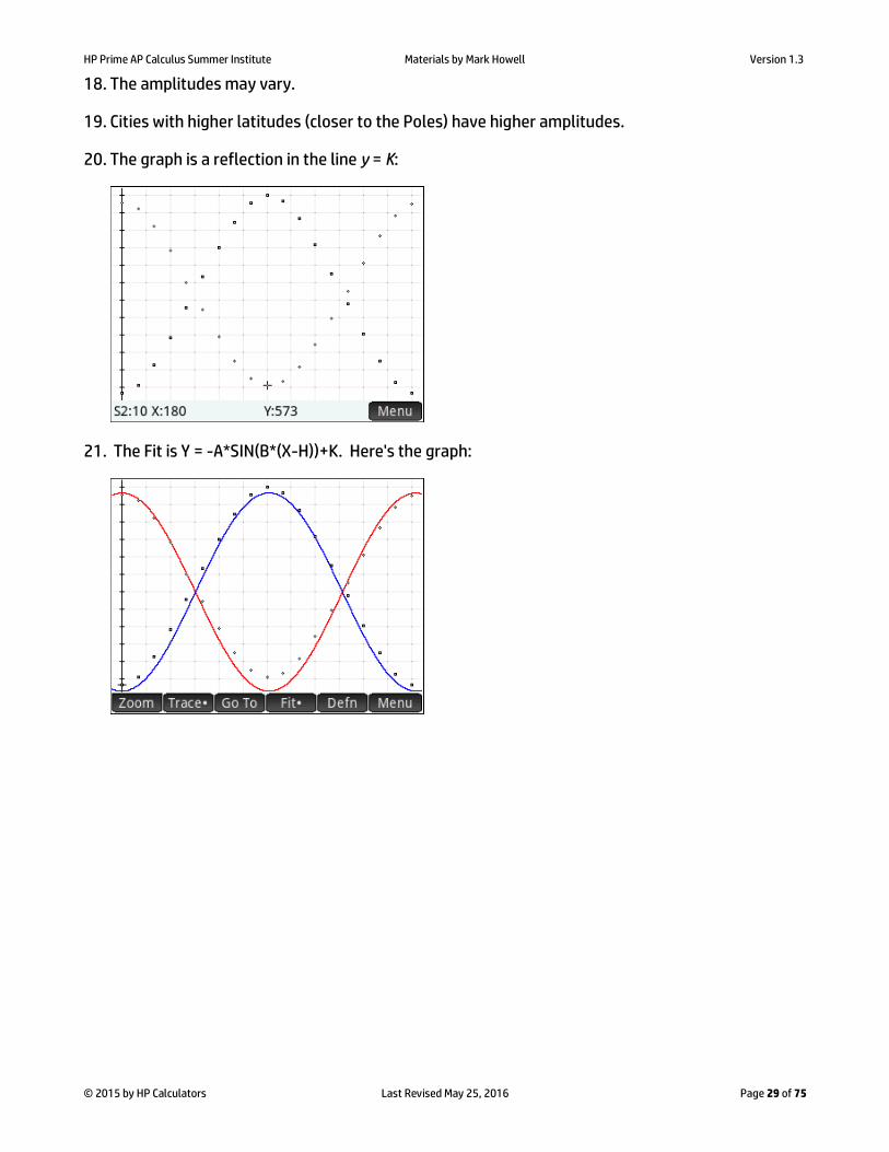
20. The graph is a reflection in the line y = K:
21. The Fit is Y = -A*SIN(B*(X-H))+K. Here's the graph:

HP Prime AP Calculus Summer Institute Materials by Mark Howell Version 1.3
© 2015 by HP Calculators Last Revised May 25, 2016 Page 30 of 75
Sunrise-Sunset Data Activity (Calculus)
HP Prime Functionality Introduced:
Using the Statistics 2Var App; using Copy and Paste; using the List command
AP Calculus Content:
This activity involves interpreting rates of change in context; it foreshadows the first derivative test;
calculation of many average rates of change; can be revisited after the chain rule is covered to make an interesting connection between the amplitude of the function L(X) in the previous activity, and the amplitude of the function R(X) in this activity
Activity:
Using the data collected from the sunrise-sunset data activity, you will explore some basic calculus
ideas. In particular, you will approximate rates of change in the number of minutes of daylight with
respect to the number of days since the winter solstice, and look for connections between these values and the particular time of year.
Let the function L(X) represent the number of minutes of daylight on day X since the winter solstice,
1. Using the data you collected (not the function you may have found to model the data), approximate the rate of change of L(X) with respect to X when X = 180 (approximately halfway through the year). Show your calculations and include units of measure.
____________________________________________________________________________
2. What time of the year is it on day 180? What seems to be true about the number of minutes of daylight on a day at this time?
____________________________________________________________________________
____________________________________________________________________________
____________________________________________________________________________

HP Prime AP Calculus Summer Institute Materials by Mark Howell Version 1.3
© 2015 by HP Calculators Last Revised May 25, 2016 Page 31 of 75
3. Again using the data you collected, approximate the rate of change of L(X) with respect to Xwhen X = 270 (approximately three-fourths of the way through the year). Show yourcalculations and include units of measure.
____________________________________________________________________________
4. What time of the year is it on day 270? What seems to be true about the number of minutesof daylight on a day at this time?
____________________________________________________________________________
____________________________________________________________________________
____________________________________________________________________________
On the Home screen, press b 6 7 to select
the List command from the toolbox. Enter the
command List(C2)/20 STO> C5. This stores into
C5 the approximate rate of change of L(X) on all of
the days you have daylight data for.

HP Prime AP Calculus Summer Institute Materials by Mark Howell Version 1.3
© 2015 by HP Calculators Last Revised May 25, 2016 Page 32 of 75
5. Set up and make a scatter plot of C5 versus C1. You'll have to delete the first entry from
C1 since there is one fewer difference in C5 than entries in C1.
6. On approximately what day X does the graph of C5 versus C1 change sign from positive to negative? What time of the year is this?
____________________________________________________________________________
____________________________________________________________________________
7. On approximately what day X does the graph of C5 versus C1 reach a maximum? What time of the year is this?
____________________________________________________________________________
____________________________________________________________________________
8. On approximately what day X does the graph of C5 versus C1 reach a minimum? What time of the year is this?
____________________________________________________________________________
____________________________________________________________________________

HP Prime AP Calculus Summer Institute Materials by Mark Howell Version 1.3
© 2015 by HP Calculators Last Revised May 25, 2016 Page 33 of 75
9. Using the techniques described in the previous sunrise-sunset data activity, determine the equation of a function in the form R(t) = C cos(D(X-E)) + F that will pass through the points in the scatter plot of C5 versus C1.
____________________________________________________________________________
10. If you did the extensions of the previous activity, describe the similarities and differences among the rates of change of minutes of daylight for DC, Honolulu, and Melbourne, Australia.
____________________________________________________________________________
____________________________________________________________________________
____________________________________________________________________________
____________________________________________________________________________
11. If you have covered the chain rule in class, compare the amplitude of this Fit with the
amplitude of the Fit of the number of minutes of daylight versus the number of days since the solstice. How are the amplitudes related symbolically? ____________________________________________________________________________
HP Prime AP Calculus Summer Institute Materials by Mark Howell Version 1.3
© 2015 by HP Calculators Last Revised May 25, 2016 Page 34 of 75
Answers
1. The approximate the rate of change of L(t) with respect to t when t = 180 is
890 888 1.05
40 20
or
890 901 11.55
20 20
or
901 888 13.65
20 20
minutes of daylight
per day
2. This is near the summer solstice, the day when the number of minutes of daylight is a maximum..
3. The approximate the rate of change of L(t) with respect to t when t = 270 is
714 7662.6
20
minutes of daylight per day
4. This is near the autumnal equinox, when there are 12 hours or 720 minutes of daylight. At this time, we lose daylight faster than at any other time of year.
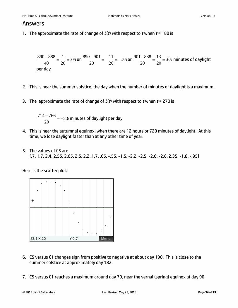
5. The values of C5 are {.7, 1.7, 2.4, 2.55, 2.65, 2.5, 2.2, 1.7, .65, -.55, -1.5, -2.2, -2.5, -2.6, -2.6, 2.35, -1.8, -.95}
Here is the scatter plot:
6. C5 versus C1 changes sign from positive to negative at about day 190. This is close to the summer solstice at approximately day 182.
7. C5 versus C1 reaches a maximum around day 79, near the vernal (spring) equinox at day 90.

HP Prime AP Calculus Summer Institute Materials by Mark Howell Version 1.3
© 2015 by HP Calculators Last Revised May 25, 2016 Page 35 of 75
8. C5 versus C1 reaches a minimum around day 265, near the autumnal (fall) equinox at day 270.
9. F = 0. The period is 365 days, so D =2*/365. The phase shift E is one quarter of a year, so E = 90. The amplitude is half the difference between the maximum and minimum values of L5,
so C = 2.625. The resulting model is y = 2.625*sin(2*/365*(x-90)). Overlaying the model on the
scatter plot produces this result:
10. The amplitude of the R(x) function is D times the amplitude of the L(x) function.

HP Prime AP Calculus Summer Institute Materials by Mark Howell Version 1.3
© 2015 by HP Calculators Last Revised May 25, 2016 Page 36 of 75
The Derivative Function
HP Prime Functionality Introduced:
Zooming in to a table; using one function to define another; using Numstep to define a function
AP Calculus Content:
Definition of derivative,
0limh
f x h f xf x
h
Activity:
Students connect to the HP Classroom Network, and
the teacher distributes the DervDefnZmTbl App. Once you have the App, press !, and select
DervDefnZmTbl. The App is based on the built-in Function App. Press @ to see the definitions of the
functions you will explore in this activity. Notice that, for the time being, F2(X) is the only function selected.
Press SN (Num Setup). There, you see values for variables that control how the Numeric View
appears, including NumStart, NumStep, and NumZoom. NumStart is the top value in the table. NumStep is the difference between adjacent inputs in the table, and NumZoom is a factor that NumStep changes by when you zoom in (divide NumStep by NumZoom) or zoom out (multiply NumStep by NumZoom).
1. What is the value of NumStep? _______________________
2. Press @ to see the definitions of the functions again. Can you predict what the graph of
F2(X) will look like? ____________________________________________________________________________
The graph of F2(X) resembles a common trigonometric function. Press P to see it.
3. What trigonometric function does the graph look like? ____________________________________________________________________________

HP Prime AP Calculus Summer Institute Materials by Mark Howell Version 1.3
© 2015 by HP Calculators Last Revised May 25, 2016 Page 37 of 75
4. Explain why the graph of F2(X) looks the way it does.
____________________________________________________________________________ ____________________________________________________________________________ ____________________________________________________________________________
If you had trouble with question 4, consider this question. When X = 0,
0 0.1 0
2 00.1
SIN SINF
. This equation should look familiar. It represents an approximation
for the derivative of a certain function at a certain value of X.
5. What function? _____________________________ What value of X? ___________________
For each value of X, F2(X) represents an approximation for the derivative.
F2(X) is not exactly the derivative, though. Press @
and look again at the function definitions. Notice that F3(X) = COS(X), and F4(X) is the difference between our approximation for the derivative and the exact
derivative. Now, you will look at the numeric view for F2(X), F3(X), and F4(X). First, select F3(X) and F4(X) by tapping the check box next to each function in the Symbolic view.
Then press N and study the table. In particular,
compare the values of F2(X) and F3(X) for the same X. The values of F4(X) represent the difference between the approximation of the derivative of SIN(X) and its exact derivative, for each value of X.
Now, you will zoom in to the table. Each time you
zoom in to the table, the variable Numstep is divided by 4 (the value of Numzoom). This causes the values of X to get closer together. But remember that the variable Numstep appears in the definition of F2(X) where you may be accustomed to seeing a variable
called h or perhaps x. Therefore, zooming in to the table should make the approximations better,

HP Prime AP Calculus Summer Institute Materials by Mark Howell Version 1.3
© 2015 by HP Calculators Last Revised May 25, 2016 Page 38 of 75
since that process makes Numstep smaller. Press and select 1 In x4. For comparison, you
can look at the table of values on the previous page.
6. At each value of X, compare the values of F2(X) and F3(X). Are they closer together? ______
7. Look at the values of F4(X). Are they larger or smaller than before? _____________________
Zoom in to the table a few more times, but don't get carried away! You can also press +as a
shortcut to zoom in, just as you can with the graph.
Press P and zoom in vertically by pinching.
Place two fingers together vertically, pause for a moment, and then move them apart vertically. You will see two vertical blue arrows indicating that a vertical zoom is active. Repeat this gesture until you can see that F4(X) is not really constantly 0. The smaller you make Numstep, the more you
have to zoom in vertically to see that F2(X) and F3(X) are different.

HP Prime AP Calculus Summer Institute Materials by Mark Howell Version 1.3
© 2015 by HP Calculators Last Revised May 25, 2016 Page 39 of 75
Answers
1. NumStep is 0.1
2. COS(X)
3. COS(X)
4. F2(X) is a difference quotient that approximates the derivative of SIN(X) at each value of X. Since NumStep is a small number, 0.1, the graph of F2 resembles that derivative.
5. SIN(X) at X = 0
6. In general, the smaller NumStep is, the closer the values of F2(X) are to COS(X). That is, the
approximation gets better as we zoom in to the table.
7. F4(X) is the error from using the difference quotient, F2(X), to approximate the derivative, F3(X). So as we zoom in, the errors get smaller.

HP Prime AP Calculus Summer Institute Materials by Mark Howell Version 1.3
© 2015 by HP Calculators Last Revised May 25, 2016 Page 40 of 75
Implicit Differentiation
HP Prime Functionality Introduced:
Advanced Graphing App; using Plot Setup variables; navigating the Catalog; using CAS to do implicit differentiation; using CAS to solve equations
AP Calculus Content:
Implicit differentiation
Activity:
The point whose coordinates are (2,0) is a point on
the ellipse 0432 22 yyxx . What is the
equation of the line tangent to the ellipse through that point?
Press ! to open the App Library and select the
Advanced Graphing app. The app opens in its
Symbolic view, where you can enter up to 10 equations or inequalities. In V1, enter the equation for our ellipse. Tap the menu keys at the bottom to enter =, X, and Y. Tap or press E when you
are done.
Press P to see the graph of the ellipse. Press +
to zoom in and drag to center the ellipse, as shown
in the figure to the right.

HP Prime AP Calculus Summer Institute Materials by Mark Howell Version 1.3
© 2015 by HP Calculators Last Revised May 25, 2016 Page 41 of 75
Move the tracer to the point (2,0) and press + to
zoom in on this point. Continue to zoom until you
have established local linearity, as in the figure to the
right.
We will now estimate the slope of the curve at (2, 0).
Press R to move the cursor one pixel to the right of
(2, 0). The current trace cursor coordinates are saved
in the variables X and Y. Press H to open Home
view. Press c to open the Template menu and
choose the fraction template. Make the numerator 0
– Y and the denominator 2 – X. Press E to see
the result as shown in the figure. Our estimate for
the slope is close to -1.
We will now use implicit differentiation to find the
slope exactly. Press C to open the CAS view. Press
b to open the Toolbox Menus, tap , then
press i m (IM) to jump to commands that start
with those two letters. Scroll down to
implicit_diff. Press ^ to view the help page
for this command. Notice the menu keys:
: opens the entire help tree
: opens a menu of examples to paste
into the CAS
: page by page navigation
: view related commands
: close the help page

HP Prime AP Calculus Summer Institute Materials by Mark Howell Version 1.3
© 2015 by HP Calculators Last Revised May 25, 2016 Page 42 of 75
We can see that the command takes an expression, followed by the variables for differentiation.
Tap to close the help page. Tap to paste
the command into the CAS. The CAS uses lower-case
variable names, so use x and y here.
Enter the expression for our ellipse, followed by both x
and y, and press E to see the result. Tap to
simplify the expression.
Press c and select the third template in the first row
(called the where() command. Tap on the first square,
then tap on our last result and tap to copy it into
the square. Tap on the second square and enter x=2,
y=0. Press E to see the result: the slope is -1.
Press @ to return to Symbolic view and enter the
equation of the tangent line. The line whose slope is -1
and contains (2, 0) is y-0= -1(x-2) or y= -x+2. Enter this
equation in V2 and press P to see the graph. You can
enter the equation in either point-slope form or slope-
intercept form. Press - to zoom back out so you can
see the entire ellipse.
Before HP Prime, using implicit differentiation to find the slope of the tangent to the graph of a
relation was a mechanical exercise with a leap of faith that the equation obtained really was the equation of a line tangent to a curve. Now we can easily verify by graphing.

HP Prime AP Calculus Summer Institute Materials by Mark Howell Version 1.3
© 2015 by HP Calculators Last Revised May 25, 2016 Page 43 of 75
Extension
Find any values of a for which the parabola 52 yax is also tangent to our line y= -x+2.
Press C to return to the CAS. Differentiate our
equation implicitly with respect to both x and y, as
shown in the figure to the right.
Press b, tap , tap Solve, and select solve.
Now copy the expression (just double-tap it) and set
it equal to -1 as shown. Press o, followed by y to
solve for y and press E to see the result.
We know that the point of tangency satisfies both
equations (the parabola and the line). Return to the
where() command and enter the parabola equation
as shown in the figure to the right. In the second
square enter the substitution x= 2-y to get an
equation in a and y.
Repeat with the result and our substitution for y in
terms of a, given by our implicit derivative equation.
Now solve for a. The result shows that there are two
values of a, -1/10 and 1/2, for which the graph of
52 yax is tangent to the line y= -x+2.

HP Prime AP Calculus Summer Institute Materials by Mark Howell Version 1.3
© 2015 by HP Calculators Last Revised May 25, 2016 Page 44 of 75
Return to Symbolic view and enter these equations in
V3 and V4.
Press P to see the graphs.
You can perform the entire process in one step if you
like. Use the solve() command with the set of
equations enclosed in curly braces as a system, followed by the vector of variables. The figure to the right shows the exact expression and the result. The result shows that:
When a = -1/10, the parabola is tangent to the line at the point (-3, 5)
When a= ½, the parabola is tangent to the line
at the point (3, -1) These results can be verified in Plot view. The HP Prime CAS gives you extraordinary flexibility in exploring and solving problems exactly.

HP Prime AP Calculus Summer Institute Materials by Mark Howell Version 1.3
© 2015 by HP Calculators Last Revised May 25, 2016 Page 45 of 75
Approximating Integrals with Riemann Sums
HP Prime Functionality Introduced:
Using a custom View menu to navigate a user App.
AP Calculus Content:
Introduction to Riemann Sums using area; convergence of Riemann Sums and behavior of their error
Activity:
Students connect to the HP Classroom Network, and the teacher distributes the NumInt App. Press !, and select NumInt. The App is based on the built-in Function App.
In this activity, you will work with the function f x x . In particular, you will approximate the
definite integral, 9
1xdx , which represents the area underneath the graph of f x from x = 1 to
x = 9.
The first step in approximating an integral is to sub-divide your interval. In this example, you're working with the interval from x = 1 to x = 9.
1. Press P and look at the graph of 1F X X .

HP Prime AP Calculus Summer Institute Materials by Mark Howell Version 1.3
© 2015 by HP Calculators Last Revised May 25, 2016 Page 46 of 75
First, you will use 2 subintervals, [1,5] and [5,9]. You'll evaluate your integrand function,
1F X X , at the left hand endpoint of each of these intervals, X = 1 and X = 5, using the
Numeric View to see the results. Press SN (Num Setup). Notice that the table setup (Num
Type) is set to Build Your Own table. Press N and enter 1 and 5 into the column for X.
2. On your graph in number 1, draw the rectangles with width 4 and heights given by the values of F1(1) and F1(5). To do this, place your pencil on the x-axis at X = 1. Draw a vertical line segment
up to the graph of F1(X). The length of that line segment is 1 1 1 1F . Then draw a
horizontal line segment from the point (1, 1) straight across to the point (5, 1). Place your pencil on the x-axis at X = 5, and repeat the process of drawing a vertical line up to the graph of F1(X),
then a horizontal line to the point 9, 5 . Complete the second rectangle by drawing a vertical
segment down to the x-axis at X = 9.
3. Press N. Write out a calculation in the form of the sum of two products that gives the sum of the areas of the two rectangles you drew in question 2. Evaluate the sum, and write down its value, accurate to three digits to the right of the decimal point.
______________________________________________________________________________
This sum is called the Left-Hand Riemann Sum with 2 subintervals for F1(X) on the interval [1,9]. Look at the rectangles you drew on your graph.
4. Is the value of your left-hand sum smaller or larger than the exact area under the graph of F1(X) from 1 to 9? Explain your answer.
____________________________________________________________________
____________________________________________________________________
____________________________________________________________________
____________________________________________________________________

HP Prime AP Calculus Summer Institute Materials by Mark Howell Version 1.3
© 2015 by HP Calculators Last Revised May 25, 2016 Page 47 of 75
To improve your approximation of the area, all you need to do is include more sub-intervals so that the width of each rectangle is smaller. First, you will use 4 rectangles, each of width 2.
5. Press SN, and change NumStep to 2.
6. On the graph, draw the 4 rectangles with width 2 and heights given by the values of F1(X) from your table, following the procedure outlined in question 2.
7. Write out a calculation in the form of the sum of four products that gives the sum of the areas of the four rectangles you drew in question 7. Also calculate the sum, accurate to three decimal places.
______________________________________________________________________________
8. Is the sum larger or smaller than the exact area under the curve? _____________________
9. Is the sum larger or smaller than the sum you calculated using only two rectangles?
________________________________
Draw a picture that supports your answer to question 9.

HP Prime AP Calculus Summer Institute Materials by Mark Howell Version 1.3
© 2015 by HP Calculators Last Revised May 25, 2016 Page 48 of 75
Generally, by taking more rectangles in the sum, you get better and better approximations. However, these calculations soon become tedious. The NumInt App will help you automate the calculations.
Press V. Select 5 Limits and enter 1 for the lower limit and 9 for the upper limit (these may
already be pre-set to the correct values). Select 4 Select Method, and 1 LEFT to do left hand Riemann Sums. Then select 3 Enter num subintervals. Enter 2 for the number of subintervals and
press . Then select 6 Plot and you will see the two rectangles drawn and the sum computed.
Compare this with your answers to questions 2 and 3. Then press and V . Repeat this
process to draw 4 rectangles and compare the results with your answers to questions 6 and 7. Then press V and select 7 Numeric Results. This takes you to the numeric view where you can enter
the number of subintervals in the X column of the table. The value of the sum is computed for the currently selected method, left or right. Enter 4 for X, and you will also see the sum displayed for 4 left hand rectangles. Use the numeric view to complete the table below for Left Hand Riemann
Sums.
10.
Number of Subintervals Left Hand Riemann Sum Right Hand Riemann Sum 8
16
32
64
128
256
512
1024
2048
11. Does it appear the values of the Left Hand Riemann Sums approach a limiting value as the number of subintervals gets larger? _______________________ If so, what is that value? ____________
On the View menu, Select 4 Select Method, and 3 RIGHT to do right hand Riemann Sums. Fill in the
right hand column in the table as before.
12. Are the Right Hand Riemann Sums larger or smaller than the exact area under the curve? _____________________

HP Prime AP Calculus Summer Institute Materials by Mark Howell Version 1.3
© 2015 by HP Calculators Last Revised May 25, 2016 Page 49 of 75
13. Explain why the Right Hand Riemann Sums decrease as the number of rectangles increases.
_______________________________________________________________________________
_______________________________________________________________________________
_______________________________________________________________________________
14. Does it appear the values of the Right Hand Riemann Sums approach a limiting value as the number of subintervals gets larger? _______________________ If so, what is that value? ____________

HP Prime AP Calculus Summer Institute Materials by Mark Howell Version 1.3
© 2015 by HP Calculators Last Revised May 25, 2016 Page 50 of 75
Answers
1.
2.
3. 4 1 4 5 12.944
4. This is smaller than the exact area under the graph. Each rectangle leaves out some of the
region under the graph of F1(X).
6.

HP Prime AP Calculus Summer Institute Materials by Mark Howell Version 1.3
© 2015 by HP Calculators Last Revised May 25, 2016 Page 51 of 75
7. 2 1 2 1.73205 2 2.23607 2 2.64576 15.228 8. Smaller 9. The sum of areas of the 4 rectangles is larger than the sum of the areas of two rectangles. The
picture below supports this conclusion.
10. Number of Subintervals Left Hand Riemann Sum Right Hand Riemann Sum
8 16.306 18.306
16 16.826 17.826
32 17.082 17.582
64 17.208 17.458
128 17.271 17.396
256 17.302 17.365
512 17.318 17.349
1024 17.326 17.341
2048 17.329 17.337
11. Yes, 17.333
12. The Right Hand Riemann Sums are larger than the area under the curve, because the integrand is
increasing.

HP Prime AP Calculus Summer Institute Materials by Mark Howell Version 1.3
© 2015 by HP Calculators Last Revised May 25, 2016 Page 52 of 75
13. As we increase the number of subintervals, the right hand rectangles include less and less "extra" area. The picture below supports this conclusion.
14. Yes; 17.333
Extensions:
E1) Repeat the activity using the midpoint rule. Like the activity, have students first produce a
table of inputs and outputs (if 2 subintervals are used over the interval x = 1 to x = 5, the
inputs should be x = 2 and x = 4). UseTblStart = 2 and ΔTbl = 2. Then change ΔTbl to 0.5.
Finally, use the calculator program and just add an extra column to the table from question 13.
E2) Investigate a function that is decreasing over the interval of integration, such as 2
0)cos(
dxx .
Ask students to predict which method, left or right hand sum, will over-approximate the integral. Alternately, ask students to produce a function g for which the left hand sum will
under-approximate 5
1( )g x dx .
E3) Repeat the activity using the trapezoid rule. Demonstrate that the trapezoid rule is equivalent
to averaging the left and right hand sums. The NUMINT program leaves in its wake the most recently calculated sums in the list variable, L6. L6(1) is the left hand sum, L6(2) the right hand sum, L6(3) the midpoint sum, and L6(4) the trapezoid sum. You could calculate (L6(1) + L6(2))/2 and compare the result to L6(4), for example.
E4) Sometime after students know how to evaluate a definite integral using the Fundamental Theorem of Calculus (so that the exact value of an integral is known), return to the NUMINT program, and use the values in L6 to explore the errors from using the various approximations.

HP Prime AP Calculus Summer Institute Materials by Mark Howell Version 1.3
© 2015 by HP Calculators Last Revised May 25, 2016 Page 53 of 75
Fundamental Theorem Investigation
HP Prime Functionality Introduced:
Defining a function in terms of an integral, the MAKELIST() and other List commands,
AP Calculus Content:
The Fundamental Theorem of Calculus
Activity:
In this activity, students explore the Fundamental Theorem of Calculus from numerical and graphical perspectives. The exploration gives students additional practice with functions of the form
0( ) ( )
x
F x f t dt .
Press ! and select the FTCFxn App. Study the function definitions in the Symbolic View.
Notice the F3(X) and F4(X) are functions defined by a definite integral. That is, the independent variable of the functions is the upper limit of integration. Also notice that that F2(X) is the only function selected for graphing. Press P and look at the graph. Your graph should look like the one shown.
Now, you will create three lists. The first list, C1, consists of values of the independent variable, X, from the graph screen. These will serve as inputs into F3(X). To create the lists, follow these steps:
Press b and the menu key, then select MAKELIST from the LIST group.
Fill in the arguments as shown at right. Press the menu key. Press Ac , then enter 1 to enter C1.

HP Prime AP Calculus Summer Institute Materials by Mark Howell Version 1.3
© 2015 by HP Calculators Last Revised May 25, 2016 Page 54 of 75
Now you will evaluate F2(X) at each of the inputs in C1, and store the results in another list, C2. Touch the MAKELIST command that you just entered with your finger to select it, and then press . Navigate to the first argument, X, and replace it with F2(X). Then navigate to the end of the edit line and replace C1 with C2. Press E to generate and store the list of outputs from F2(X) into the C2.
Repeat this procedure to evaluate F3(X) at each of the inputs and store the results in list C3 as shown.
Remember that each element of C3 results from the evaluation of a definite integral. For example, when 0.05, the second value of C1 is plugged into F3(X), the value of
20.05
0cos 0.04999992
2
TdT
results, which is the second value in C3. 1. Explain why the first value in C3, which results from evaluating F3(0), is 0.
__________________________________________________________________________________ Press P and look at the graph of the integrand, F2(X). Use the graph to answer questions 2 and 3. 2. Why is the second value in C3 greater than 0? __________________________________________ __________________________________________________________________________________

HP Prime AP Calculus Summer Institute Materials by Mark Howell Version 1.3
© 2015 by HP Calculators Last Revised May 25, 2016 Page 55 of 75
3. Why is the third value in C3, which represents 2
0.1
03 0.1 cos
2
TF dT
, greater than the second
value in C3, which represents 2
0.05
03 0.05 cos
2
TF dT
?________________________________
__________________________________________________________________________________ __________________________________________________________________________________ Press ! and select Statistics 2Var to see a table of inputs and outputs. Remember that C1
contains the X values; C2 contains the values of the integrand, cosT 2
2
; and C3 contains the values
of the integral, 2
0cos
2
X TdT
. Use the cursor keys or swipe with your finger to navigate down the
C3 column. 4. From the list of data values stored in C3 for what value of X (stored in C1) does
2
03( ) cos
2
X TF X dT
appear to reach its first local maximum?
__________________________
5. Explain why the 38th value is smaller than the 37th value in C3. That is, why is 2 2
1.85 1.8
0 0cos cos
2 2
T TdT dT
?
__________________________________________________________________________________ __________________________________________________________________________________ __________________________________________________________________________________ 6. From the list of data values stored in C3, for what positive value of X does
2
03( ) cos
2
X TF X dT
appear to reach its first local minimum?
__________________________ Press ! and select FTCFxn to return to the FTCFxn App, and look at the plot of the integrand
again. Press , , and select 2 Root. Move the cursor close to the smallest x-intercept on the graph of F2(X) . 7. Record the x-intercept. _________________________________________________
8. Move the cursor close to the next largest x-intercept, and use the Root command to find it. Record the next largest x-intercept. ______________________________________

HP Prime AP Calculus Summer Institute Materials by Mark Howell Version 1.3
© 2015 by HP Calculators Last Revised May 25, 2016 Page 56 of 75
Compare these Roots to your answers to numbers 4 and 6. 9. Find the next positive X-intercept of the graph of F2(X) (close to X = 4). __________________ 10. What happens with F3(X) at the point found in question 9? _______________________________ __________________________________________________________________________________ Verify your answer numerically by going back the Statistics2Var App and looking at the table of values for F3(X) in C3. Press H, copy the most recent MAKELIST command to the edit line, and change the arguments as shown to evaluate F4(X) at all the inputs in C1 and store the results in C4.
Now you'll create scatter plots of C3 versus C1 and C4 versus C1. Press ! and select Statistics 2Var. Press @to start the Symbolic View. Enter the setups shown in the screens below.

HP Prime AP Calculus Summer Institute Materials by Mark Howell Version 1.3
© 2015 by HP Calculators Last Revised May 25, 2016 Page 57 of 75
Then press S# to go to the Plot Setup View. Enter the settings shown.
Press # to see the graph.
Note that the first element of C4 represents 2 2
0 1
1 04(0) cos cos
2 2
T TF dT dT
.
11. Why is the graph of C4 versus C1 (in scatter plot S2) below the graph of C3 versus C1 (in scatter plot S1)? (Remember, the only difference between the definitions of F3 and F4 is the lower limit of integration.)
__________________________________________________________________________________ __________________________________________________________________________________ 12. It appears that corresponding values in C4 and C3 differ by a constant, i.e. that F4(X) – F3(X) is
the same for all values of X. Find the value of this constant.
_________________________________________________________
(You could calculate this in several different ways. If you get stuck, try expressing F4(X) – F3(X) in terms of an integral.)

HP Prime AP Calculus Summer Institute Materials by Mark Howell Version 1.3
© 2015 by HP Calculators Last Revised May 25, 2016 Page 58 of 75
13. Explain why plots S1 and S2 have the same shape. __________________________________________________________________________________ __________________________________________________________________________________ __________________________________________________________________________________ Press $ and look at the table of values for C3 and C4, and notice that the locations of the extrema are the same for both functions (as you would expect from an inspection of the scatter plots).
14. Look at the locations of the local minima and the local maximum on the graph of F2(X). At these
values of X, describe what appears to happen with the concavity of the graphs from S1 and S2. __________________________________________________________________________________ __________________________________________________________________________________ __________________________________________________________________________________ 15. Write an equation with a derivative on one side that shows how F2(X) and F3(X) are related. __________________________________________________________________________________ 16. Recall that the derivative of a function f at x = a can be defined by
f (a) limxa
f (x) f (a)
x a. Approximate F3'(1) by evaluating the expression (F3(1.1) – F3(1))/0.1.
_________________. Your answer should be close to the value of F2(1). Why? _______________________________________________________________________________ _______________________________________________________________________________ _______________________________________________________________________________
17. Approximate F4'(1)by evaluating the expression (F4(1.1) – F4(1))/0.1. _________________. Again, your answer should be close to the value of F2(1). Why? _______________________________________________________________________________ _______________________________________________________________________________

HP Prime AP Calculus Summer Institute Materials by Mark Howell Version 1.3
© 2015 by HP Calculators Last Revised May 25, 2016 Page 59 of 75
Extension
This extension is a must-do!
After students have seen that 3( ) 2( )d
F X F XdX
, or 2 2
0cos cos
2 2
Xd T XdT
dX
, it is natural
to gather more evidence in support of this conclusion. Because we have assembled data of inputs and outputs for F3, and we have a formula for F2, it is a relatively simple matter to form difference quotients for F3 and compare them to outputs from F2. This was done for a single value of X in question 16. Here's one way to do it for all the values of F3 that we've calculated. You will form the difference quotients using the calculator's List command. That command generates a new list, with each entry formed by subtracting adjacent pairs of the argument. On the Home screen, press b 6 1 to select the List command. Enter the command List(C3)/0.05 C5. Applying the List command to the list, C3, and then dividing that list by the differences in the input list, 0.05, gives a list of difference quotients. The list C5 contains one entry fewer than C1, C2, C3, and C4. So, you need to manually calculate and enter the missing value at the end of C5. Note that it should represent the average rate of change of F3 on the interval from X = 5.3 to X = 5.35. So it is
2 2 25.35 5.30 5.35
0 0 5.30cos cos cos
2 2 2
0.05 0.05
T T TdT dT dT
. Position the cursor in the cell for
C5(107) and enter that expression, as shown.

HP Prime AP Calculus Summer Institute Materials by Mark Howell Version 1.3
© 2015 by HP Calculators Last Revised May 25, 2016 Page 60 of 75
Then set up a scatter plot of C5 versus C1, and behold!

HP Prime AP Calculus Summer Institute Materials by Mark Howell Version 1.3
© 2015 by HP Calculators Last Revised May 25, 2016 Page 61 of 75
Answers
1. The first value in C3 represents 0
02( )Y T dT and so is zero. There is no area from 0 to 0.
2. The second value in C3 is positive since the integrand is positive for all T in the interval
[0, 0.1].
3. The third value in C3 is greater than the second since the integrand is positive for all x in the interval [0.1, 0.2].
4. 1.8
5. cosT 2
2
dT
0
1.9
cosT 2
2
dT
0
1.8
because the integrand is negative for all T in the interval
[1.8, 1.9]. Thus, the function is decreasing.
6. 3.1 In questions 7-10, students should observe that the function F3 has a maximum where the
integrand changes sign from positive to negative, and a minimum where the integrand changes sign from negative to positive. Again, this connection is meant to recall students' experience with the locations of maximum and minimum points and their relationship with the sign of the derivative. A question like, “Have you ever seen a situation in which one ‘thing’ reaches a maximum where another ‘thing’ changes sign from positive to negative? What are the two ‘things’?” Students make the connection explicit in question 15.
7. (A) 1.77245 and (B) 3.06998
8. At the first x-intercept, 1.77245, the integrand changes sign from positive to negative. Thus
the function, F3, has a local maximum there. We stop accumulating positive values of F2, and start accumulating negative values at that point. Similarly, at x = 3.06998, the integrand changes sign from negative to positive. Thus, we stop accumulating negative values and start accumulating positive values at that point, producing a local minimum on the graph of F3.
9. 3.963327
10. F3 has a maximum there. Looking at the table of values for C1, C2, and C3, this occurs near X = 4.
11. Answers will vary. Focusing on X = 0, 2
0
03(0) cos
2
TF dT
is zero, since the upper and
lower limits of integration are equal. However, 2 2
0 1
1 04(0) cos cos
2 2
T TF dT dT
< 0,
since the integral is positive. This puts the graph of C4 below the graph of C3. Also see the answer to question 12.

HP Prime AP Calculus Summer Institute Materials by Mark Howell Version 1.3
© 2015 by HP Calculators Last Revised May 25, 2016 Page 62 of 75
12. The difference is a constant. Just calculate F4(0) – F3(0) = –0.975288. Students may notice that
F4(X)-F3(X) = cosT 2
2
dT
1
X
cosT 2
2
dT
0
X
cosT 2
2
dT
0
1
and simply evaluate the
latter integral, or note that it is the negative of C4(1). The punch line is at hand in question 13! The Fundamental Theorem says that the two functions, F3 and F4, have the same derivative, F2. The derivative of a function tells you the slope on the graph of the function, and graphs that have the same slope everywhere have the same shape. In fact, S1 and S2 are members of the family of antiderivatives of F2. Two antiderivatives of a function always
differ by a constant.
13. S1 and S2 have the same shape since each accumulates the same amount of area from the graph of F2 as X increases. So each increases at the same rate where the integrand is positive, and each decreases at the same rate where the integrand is negative.
If you have addressed the connection between points of inflection and extrema of the first derivative (in addition to the more customary definition as points where the second derivative changes sign), then question 14 should give students yet another indicator that F2 is indeed the derivative of F3.
14. The graphs of S1 and S2 both appear to have a change of concavity at the points where the graph of F2 has a local maximum or a local minimum. The points of inflection occur at X = 2.506629, X = 3.544908, and X = 4.341608. These are the extrema on the graph of F2.
15. 3( ) 2( )d
F X F XdX
or better stated, 2 2
0cos cos
2 2
Xd T XdT
dX
.
Questions 16 and 17 lead students to approximate the derivative of F3 by forming difference quotients. The answers are not exactly the same as the output from F2. To get better agreement,
you could have students form a difference quotient with a smaller step size as follows:
Evaluate 3(1.0001) 3(1)
0.0001
F YF, and compare it to F2(1). They agree to four digits to the right of the
decimal!
16. (F3(1.1) – F3(1))/0.1 = 0.851261. F2(1) = 0.877583
17. (F4(1.1) – F4(1))/0.1 = 0.851261. F2(1) = 0.877583
Notice that the difference quotients are identical. F3 and F4 are changing by exactly the same amount, an amount dictated by the magnitude of F2.

HP Prime AP Calculus Summer Institute Materials by Mark Howell Version 1.3
© 2015 by HP Calculators Last Revised May 25, 2016 Page 63 of 75
Differential Equations and Slopefields
HP Prime Functionality Introduced:
Using CAS to solve a differential equation
AP Calculus Content:
Differential equations, slope fields, Euler's Method
Activity:
Students connect to the HP Classroom Network, and the teacher distributes the DiffEqWithSlopeFields App. Once you have the App, press !, and select
DiffEqWithSlopeFields. The App is based on the built-in Statistics 2Var App. Press V and select 1
Start to see a note describing how to use the App. Many of the user interactions occur from the View
menu. Notice that the App uses a slope expression in terms of X and/or Y that is defined in the Function App as F1(X).
So, press !, and select Function. Define
1F X X . By doing so, within the
DiffEqWithSlopeFields App, you will be working with
the differential equation dy
xdx
. Press !, and
select DiffEqWithSlopeFields. Then press V. The
DiffEqWithSlopeFields App gives you the opportunity to explore differential equations graphically, numerically, and symbolically.
First, let's look at the slope field. Before you draw the slope field, think about the differential equation.
1. Will the slope segments in the slope field be positive or negative?
____________________________
2. What should the slope field show for X < 0? ____________________________________
Select 2 Slope Field and look at the slope field.
3. What happens to the slopes as X increases? _____________________________________

HP Prime AP Calculus Summer Institute Materials by Mark Howell Version 1.3
© 2015 by HP Calculators Last Revised May 25, 2016 Page 64 of 75
Notice that the slopes are the same within the same column and change as you move across the field (that is, slope depends only on X ). Later, you will see an example where the slopes are the
same within the same row and change as you move up and down in the field (slope depends only on Y ). In other examples, slopes change as you move vertically or horizontally in the field (slope depends on both X and Y ).
Now let's take a quick look at how Euler's Method works. Though this is not a topic covered in AP Calculus AB, doing so let's us explore a numeric method for solving differential equations. Moreover,
Euler's Method as you will see is really just a running left-hand Riemann Sum (a topic which is a part of AP Calculus AB).
The idea of Euler's Method is this. At any point in the plane (and we start at some chosen point, the
initial condition of the differential equation), we can calculate slope using the differential equation. With that point and slope, we find the equation of a line, and use that equation to find another point
a distance of X away (we keep X constant). At the new point, we use the differential equation to
calculate slope again, and then find an equation of another line. We use that line to find a third point
a distance of X away. We repeat the process until we reach some predetermined final value of X.
Using a linear equation to calculate a new value for Y each time comes down to this formula:
new oldY Y slope X .
Let's apply this process with the differential equation dy
xdx
with an initial condition of 1,0 .
We'll approximate y when x = 9, using two equal steps. This makes x = 4. We start at 1,0 .
4. What is the slope at 1,0 ? __________________________
Now using the formula new oldY Y slope X to calculate the new y, we have 0 1 4 4newY . Our
new point is 5,4 .
5. What is the slope at 5,4 ? __________________________
Again using the formula new oldY Y slope X , we calculate the new y. Use the Home screen to
calculate the new Y.
6. What is the approximate value of Y when X = 9 ?________________________________
Press V and select 6 Euler Setup. Enter the
parameters shown in the screen at right. These were determined by the initial condition, (1, 0) , the final X, 9, and the number of steps, 2. Then select 3 Euler Numeric. Compare the value displayed with
your answer to question 6. They should be the

HP Prime AP Calculus Summer Institute Materials by Mark Howell Version 1.3
© 2015 by HP Calculators Last Revised May 25, 2016 Page 65 of 75
same. Select 4 Euler Plot to see a scatter plot of the three points. Trace on the scatter plot, and
you'll see the coordinates of the three points.
Apply Euler's Method with the same differential equation and initial condition, but this time using 4 steps instead of two.
7. Complete this table. The first step has been done for you.
,old oldX Y Slope new oldY Y slope X ,new newX Y
1,0 1 0 1 2newY 3,2
3,2
Press V and select 6 Euler Setup. Change x to 2. Then select 3 Euler Numeric. Compare the
value displayed with your final y. They should be the same. Select 4 Euler Plot to see a scatter plot of the points. Adjust the viewing window appropriately, then press V and select 5 Overlay Field.
You'll see a slope field on top of the Euler Plot. Trace on the scatter plot to check your answers.
Now, go back to the Riemann Sum activity and compare these calculations with those that answered questions 3 and 7.
8. What do you notice? ___________________________________________________________
Solve this differential equation analytically using separation of variables.
9. What is the solution? __________________________________________________________
Press @ and enter the solution into Fit1. Press and select 5 OverlayField. Behold! A
graphic, numeric, and analytic perspective on the solution of a differential equation!
Press D to trace on the Fit. The press 9 E to jump to the point where x = 9.
10. What is the exact value of y when x = 9? _______________________________
Notice that our slope function is increasing on the interval from x = 1 to x = 9. This means that the solution curve is concave up.
11. Whenever the solution curve is concave up, will Euler's Method result in an over- or under- approximation of the exact function value? ______________________________

HP Prime AP Calculus Summer Institute Materials by Mark Howell Version 1.3
© 2015 by HP Calculators Last Revised May 25, 2016 Page 66 of 75
Recall from the Riemann Sum activity that when the integrand was increasing, left hand sums will under-approximate the exact area under the curve. Notice the connection!
HP Prime will solve differential equations analytically. Press C. Then press b and select 3 Solve and 6 Differential Equation.
Enter the command shown on the figure at right. Use the A shift key to enter y, and S a
(Chars) to find the ' character. The word "and" can be entered in lower case. Enter it manually or press S 6 to open a menu of Boolean operators.

HP Prime AP Calculus Summer Institute Materials by Mark Howell Version 1.3
© 2015 by HP Calculators Last Revised May 25, 2016 Page 67 of 75
Extension
Use the DiffEqWithSlopeFields app to explore and solve this differential equation:
12. 1
2
dy y
dx
with initial condition 3, 4 .
(a) Approximate y when x = 3 using Euler's method with 12 equal steps. _________________
(b) Solve the differential equation analytically, and overlay the solution, slope field, and Euler Plot.
_________________________________________________________________________
(c) Does Euler's Method under- or over-approximate the solution? Why?
_________________________________________________________________________ _________________________________________________________________________ _________________________________________________________________________

HP Prime AP Calculus Summer Institute Materials by Mark Howell Version 1.3
© 2015 by HP Calculators Last Revised May 25, 2016 Page 68 of 75
Answers
1. Positive
2. Since dy
dx is undefined when x < 0, there should be no slope segments there.
3. As x increases, the slopes increase.
4. At 1,0 the slope is 1
5. At 5,4 the slope is 5 2.2361
6. When X = 9, Y is approximately 12.9443
7.
,old oldX Y Slope new oldY Y slope X ,new newX Y
1,0 1 0 1 2newY 3,2
3,2 3 2 3 2newY 5,5.4641
5,5.4641 5 5.4641 5 2newY 7,9.9362
7,9.9362 7 9.9362 7 2newY 9,15.2277
8. The calculation of the left hand Riemann Sum to approximate 9
1xdx using 4 rectangles of
equal width is identical to the Euler's Method calculations in the table.
9. The solution is 3/22 2
3 3y x .
10. When x = 9, y = 17.3333 (notice that this is the same as 9
1xdx ).
11. When the solution curve is concave up, Euler's Method will result in an under-
approximation of the exact function value.
12. (a) The approximation is 0.8733

HP Prime AP Calculus Summer Institute Materials by Mark Howell Version 1.3
© 2015 by HP Calculators Last Revised May 25, 2016 Page 69 of 75
(b) The solution is 2
3
251
X
ey . Here's the graph
(c) Euler's Method over-approximates the solution, since the graph of the solution is concave
down.
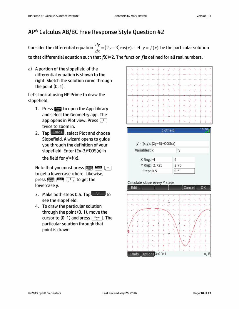
HP Prime AP Calculus Summer Institute Materials by Mark Howell Version 1.3
© 2015 by HP Calculators Last Revised May 25, 2016 Page 70 of 75
AP® Calculus AB/BC Free Response Style Question #2
Consider the differential equation )cos(32 xydx
dy . Let )(xfy be the particular solution
to that differential equation such that f(0)=2. The function f is defined for all real numbers. a) A portion of the slopefield of the
differential equation is shown to the right. Sketch the solution curve through
the point (0, 1).
Let’s look at using HP Prime to draw the
slopefield.
1. Press ! to open the App Library
and select the Geometry app. The app opens in Plot view. Press +
twice to zoom in.
2. Tap , select Plot and choose Slopefield. A wizard opens to guide
you through the definition of your slopefield. Enter (2y-3)*COS(x) in
the field for y′=f(x).
Note that you must press A S x
to get a lowercase x here. Likewise, press A S y to get the
lowercase y.
3. Make both steps 0.5. Tap to
see the slopefield. 4. To draw the particular solution
through the point (0, 1), move the cursor to (0, 1) and press E. The
particular solution through that point is drawn.

HP Prime AP Calculus Summer Institute Materials by Mark Howell Version 1.3
© 2015 by HP Calculators Last Revised May 25, 2016 Page 71 of 75
b) Write an equation for the line tangent to the solution curve in part (a) at the point (0, 1).
Use the equation to approximate f(0.2).
5. Press C to open CAS view. Enter
our expression for dy/dx. Press c
and choose the Where command:
. Enter the conditions, as shown in the figure to the right.
6. The result shows that the slope of
our tangent line is -1 and that it also contains the point (0, 1). The equation is then y= -1x+1. When x is 0.2, y= 0.8.
c) Find y=f(x), the particular solution to the differential equation with the initial condition f(0)=1.
7. Return to CAS view. Press b to
open the Toolbox Menus. Tap
to open the CAS menu. Tap Solve and select Differential
Equation. Enter the differential
equation in the form y′=f(x, y) and
the initial conditions with AND between them. Press S a to
find the y′ symbol; press S 6
to find the AND Boolean operator.

HP Prime AP Calculus Summer Institute Materials by Mark Howell Version 1.3
© 2015 by HP Calculators Last Revised May 25, 2016 Page 72 of 75
8. Press E to see the result.
We will now plot the graph of our solution over the slopefield.
9. Tap on the solution expression to select it. Press S V (Copy) to
copy the solution expression to the clipboard.
10. Press @ to open Symbolic view.
Tap on the third row (the first empty
row) and tap . Tap , select Plot and choose Function.
With the cursor between the parentheses, press S M (Paste)
to paste our solution into the
plotfunc command. Tap . 11. Choose a color for the graph of our
function plot and then press P to
see the graph. 12. We can also solve the differential
equation step by step in CAS. From
the separation of variables, we have
dxx
y
dy)cos(
32. Enter the
equation in CAS and press E to
see the result. Press x 2 to
multiply both sides of the equation by 2, as shown in the figure.
13. When y=1, |2*y-3| = 3 – 2*y. Copy the expression to the command line and make the replacement above. In this case, just delete |2*y-3| and enter (3-2*y).
14. Take e raised to Ans (Press S j
for e^ and press S + for Ans).
Then subtract 3 from the result and divide that result by -2. The final result matches our expectations.
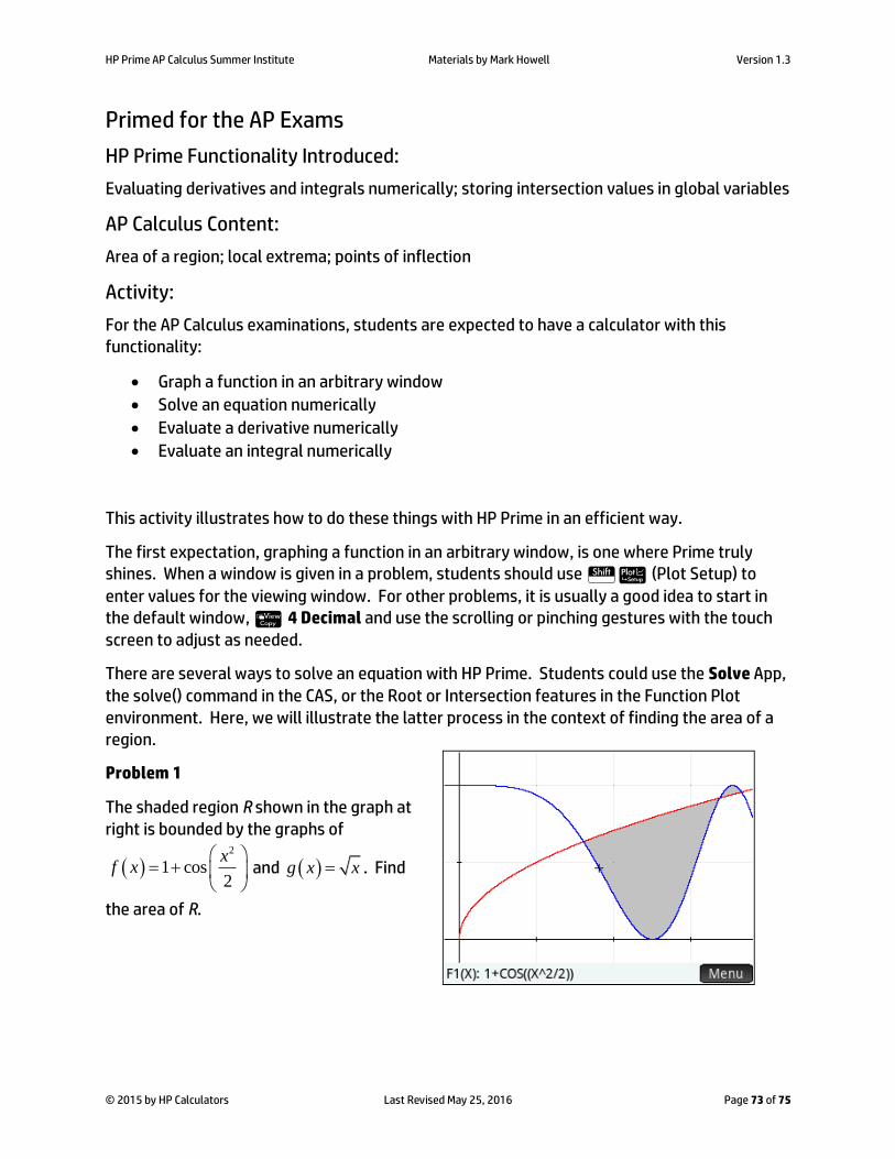
HP Prime AP Calculus Summer Institute Materials by Mark Howell Version 1.3
© 2015 by HP Calculators Last Revised May 25, 2016 Page 73 of 75
Primed for the AP Exams
HP Prime Functionality Introduced:
Evaluating derivatives and integrals numerically; storing intersection values in global variables
AP Calculus Content:
Area of a region; local extrema; points of inflection
Activity:
For the AP Calculus examinations, students are expected to have a calculator with this functionality:
Graph a function in an arbitrary window
Solve an equation numerically
Evaluate a derivative numerically
Evaluate an integral numerically
This activity illustrates how to do these things with HP Prime in an efficient way.
The first expectation, graphing a function in an arbitrary window, is one where Prime truly shines. When a window is given in a problem, students should use SP (Plot Setup) to
enter values for the viewing window. For other problems, it is usually a good idea to start in the default window, V 4 Decimal and use the scrolling or pinching gestures with the touch
screen to adjust as needed.
There are several ways to solve an equation with HP Prime. Students could use the Solve App,
the solve() command in the CAS, or the Root or Intersection features in the Function Plot environment. Here, we will illustrate the latter process in the context of finding the area of a region.
Problem 1
The shaded region R shown in the graph at right is bounded by the graphs of
2
1 cos2
xf x
and g x x . Find
the area of R.

HP Prime AP Calculus Summer Institute Materials by Mark Howell Version 1.3
© 2015 by HP Calculators Last Revised May 25, 2016 Page 74 of 75
Prime Solution
Start the Function App, if necessary, and press SP (Plot Setup). Enter a viewing window
consistent with the given graph. A horizontal view of [-0.2, 4] and a vertical view of [-0.2, 2.3] would be appropriate. Press @and enter
2
1 cos2
xf x
as F1(X) and g x x as
F2(X), then press P. In order to find the
area, we'll need to find the x-coordinates of the three points where the graphs intersect. We'll
store these into global variables so we can use
them later. First, tap the screen near the leftmost point of intersection to move the trace
there. Then press and then press
and select 2 Intersection . When
prompted, select the intersection of F1(X) and F2(X). HP Prime finds the intersection closest to the cursor (here, X = 1.61126). Immediately after the intersection is found, press Hand
press X A. Press P, tap the screen
near the second point of intersection, and
repeat the process, storing the resulting X coordinate in B. Store the third intersection in C.
Now we'll evaluate integrals to get the area. We could do this either on the Plot screen, or in
Home. We'll show how to do it in Home, since students need to write down their setups on the AP Exam anyway. Press cand tap the
template for the definite integral, in the second row, fourth column. Use the cursor keys to navigate the template and enter the integral as shown. Then press +, select the integral
template again, and enter the integral that gives the area of the second part of the region. See the screen at right. If your answer is smaller than 1.661, you probably subtracted in the integrand in reverse order.

HP Prime AP Calculus Summer Institute Materials by Mark Howell Version 1.3
© 2015 by HP Calculators Last Revised May 25, 2016 Page 75 of 75
Problem 2
Finally, here's a quick problem that illustrates how to evaluate a derivative numerically with HP Prime. Recall the function from the Sunrise-Sunset (Precalculus) activity that modeled the number of minutes of daylight as a function of the number days since the winter solstice. We
had 170.5 sin 0.0172142 91.25 730.5L xx . On the 900th day after the winter
solstice, was the amount of daylight increasing or decreasing? Justify your answer.
Prime Solution
Enter the formula for L x in the function
App as F3(X). Then on the Home screen, store
900 in the variable X by pressing 900 X. Press cand tap the template for the
derivative, in the first row, fourth column. In the top space, enter F3(X), and in the bottom, enter X. Press Eto evaluate. We see that
900 0.627 0L . Since this is positive,
the amount of daylight is increasing on day 900.
HP Prime has the ability to calculate the derivative symbolically as well. The place to do this is in the CAS. We can use the Copy and
Paste feature to copy results back to the Function App. Press C, and enter the
expression shown in the screen at right. Note again that the CAS uses lower case variables.
Incidentally, remember the Sunrise-Sunset (Calculus) activity? The value we got for the
amplitude of the fit to the scatter plot of the average rates of change of L(X) versus X was A=2.625. Compare this to what the chain rule gives us when we differentiate our model, L(X), 2.935. Pretty close!