Table of content no 4 - Energy / CIE · results of switching the power transformers and...
67
201
Transcript of Table of content no 4 - Energy / CIE · results of switching the power transformers and...

201

Editorial Board
JOURNAL OF SUSTAINABLE ENERGY EDITOR IN CHIEF Felea Ioan – Member of I.E.E.E.
University of Oradea, Department of Energy Engineering, [email protected]
EDITORS Gleb Drăgan
Member of Romanian Academy Florin Gheorghe Filip
Member of Romanian Academy [email protected]
Cornel Antal University of Oradea, [email protected]
Anatolie Carabulea Politehnica University of Bucharest
Gianfranco Chicco Politecnico de Torino , Italia [email protected]
Roberto Cipollone(details) University of L’Aquila
Fiodor Erchan State Agricultural University, Moldova
Mihai Jădăneanţ Politehnica University of Timisoara
Ştefan Kilyeni Politehnica University of Timisoara
Gheorghe Lăzăroiu Politehnica University of Bucharest
Carlo Mazetti La Sapienza di Roma
Victori�a Rădulescu Politehnica University of Bucharest
Florin Popenţiu University of Oradea
Jacques Padet Universite de Reims, France [email protected]
Paulo F. Ribeiro (details) Grand Rapids, Michigan
Marcel Roşca University of Oradea [email protected]
Saroudis J. AECL, CANDU Services
Takács János (details) Technical of University Bratislava
Victor Vaida University of Oradea [email protected]
Varju György (details) Budapest University of Technology&Economics
Kalmar Ferenc University of Debrecen [email protected]
Mircea Vereş University of Oradea [email protected]
Alexandru Vasilievici Politehnica University of Timisoara
Badea Gabriela University of Oradea, [email protected]
Nikolai Voropai Energy Systems Institute, Russia
Irena Wasiak (details) Technical University of Lodz
Dan Zlatanovici ICEMENERG
Gabriel Bendea University of Oradea
Nicolae Coroiu University of Oradea
Laurenţiu Popper University of Oradea
Călin Secui University of Oradea [email protected]
Zétényi Zsigmond
University of Oradea [email protected]
EXECUTIVE STAFF
Executive Editor: Dziţac Simona
University of Oradea, [email protected]
Editorial secretary Albuţ-Dana Daniel
University of Oradea, [email protected]
Technical Secretary Vasile Moldovan
University of Oradea, [email protected]
Editorial Activities Barla Eva
University of Oradea, [email protected]
PUBLISHER & EDITORIAL OFFICE University of Oradea Editing House,
Str. Universitatii Nr. 1, Oradea, jud. Bihor, România, Zip code: 410087, Tel.: 00-40-259-408171, Fax: 00-40-259-408404 ISSN: 2067-5534 (print version)
202

The Journal of Sustainable Energy (JSE) had its first appearance under this name in 2010. The history of JSE is the following: is formed in 2010 by transforming of 1993-2009 Analele Universitatii din Oradea. Fascicula de Energetica, 1224-1261. Which superseded in part (1991-1992): Analele Universitatii din Oradea. Fascicula Electrotehnica si Energetica (1221-1311); Which superseded in part (1976-1990): Lucrari Stiintifice - Institutul de Invatamant Superior Oradea. Seria A, Stiinte Tehnice, Matematica, Fizica, Chimie, Geografie (0254-8593);
The Journal of Sustainable Energy (JSE) publishes original contributions in the field of the following topics: Energy engineering education System reliability and power service quality Generation of electric and thermal power Energy policy and economics Energy development (solar power, renewable energy, waste-to-energy systems) Energy systems operation Energy efficiency, reducing consumption for conservation of energy Energy sustainability as related to energy and power production, distribution and usage Waste management and environmental issues Energy infrastructure issues (power plant safety, security of infrastructure network) Energetic equipments The articles quality increases with every issue. Apart from its improved technical contents, a special care is given to
its structure. The guidelines for preparing and submitting an article were modified and developed in order to meet high quality standards requirements. With every passing issue the peer-review process was developed too, being now a double-blinded peer-review process.
Authors who wish to submit a manuscript to the Journal of Sustainable Energy (JSE) are kindly asked to send their
manuscripts as DOC and PDF format to [email protected], according to the formatting instructions. Once the manuscript is submitted, the authors will shortly receive a feedback regarding the status of their submission. As the review process is completed, the author will be informed about the reviewers’ comments and the changes the paper should suffer in order to satisfy the journal quality requirements.
Journal of Sustainable Energy JSE is covered/indexed/abstracted in: Index Copernicus Ulrich's Update - Periodicals Directory DOAJ - Directory of Open Access Journals EBSCO Publishing - EBSCOhost Online Research Databases Engineering village (Pending)
The JSE may be purchased based on annual subscription (4 issues) at the following prices: paper – 50 � ,
electronic – 20 �, or individually (each number) at the following prices: paper - 20 �, electronic – 8 �. To purchase the complete “control” standard (www.energy-cie.ro) and submitted electronically or by fax. In order to generate the invoice (www.energy-cie.ro) is transmitted to the applicant. After payment of the amount stated in the bill the applicant receives and invoice numbers ordered JSE. Publishing House name/address: University of Oradea Editing House Universitatea din Oradea, Universitatii Str., No. 1, 410087, Oradea, Bihor, Romania
ISSN: 2067-5534 Tel.: 00-40-259-408171 (231, 288) Fax: 00-40-259-408404 Place of publishing: Oradea, Romania Year of the foundation of publication in domain of power engineering: 1976 Releasing frequency: 4 / year Language: English
203

CONTENTS RELIABILITY AND SYSTEMS ENERGY QUALITY SERVICES VOLTAGE QUALITY ANALYSIS IN A NETWORK POINT OF INTEREST LEŞE D., MAIER V., PAVEL S.G., BELEIU H.G.............................................................................................................................205 SENSITIVITY ANALYSIS OF RELIABILITY FOR A TYPE STRUCTURE OF THE ELECTRICAL DISTRIBUTION STATION SECUI D.C., BENDEA G. ..................................................................................................................................................................211 PRINCIPLES OF EVALUATION OF RELIABILITY OF THE EQUIPMENT OF THE POWER ELECTRICAL DISTRIBUTION SYSTEMS LUKYANENKO E..............................................................................................................................................................................215 RENEWABLE SOURCES OF ENERGY. SUSTAINABLE ENERGY TECHNOLOGIES GROUND-MED PROJECT AT THE UNIVERSITY OF ORADEA BENDEA C., ROSCA M., KARYTSAS K., BENDEA G. .................................................................................................................218 THERMAL STORAGE COUPLED TO A GROUND SOURCE HEAT PUMP IN A PUBLIC SERVICES BUILDING CARVALHO A., QUINTINO A., FONG J. AND DE ALMEIDA A.................................................................................................228 EXPERIMENTAL STUDY ON POWER CHARACTERISTIC CURVES OF A PORTABLE PEM FUEL CELL STACK IN THE SAME ENVIRONMENTAL CONDITIONS CATARIG (RUS) T., RUS L.F. ..........................................................................................................................................................232
EVOLUTION OF POWER ELECTRIC SYSTEMS TRANSPORT AND DISTRIBUTION. ENERGY SYSTEM’S PERFORMANCE THE LOAD FREQUENCY CONTROL SIMULATION OF A THERMAL GENERATOR I NTERCONECTED ON AN INFINITE BUS BARS IOVAN G., POPESCU D., MIRCEA I., .............................................................................................................................................238 THE ENERGY PERFORMANCE OF THE MAIN CONSUMERS OF THE INTERNAL SERVICES AFFERENT OF AN ENERGY BLOCK BY 330 MW POPESCU N., DINU R.C., MIRCEA I., BRATU C. ...........................................................................................................................246 VARIATION OF ELECTRICAL PARAMETERS OF TWO PUBLIC LIGHTING SOLUTIONS DUE TO CONTINUOUS DIMMING OF LIGHT OUTPUT VASILIU R.B., CHINDRIŞ M., CZIKER A., GHEORGHE D. ........................................................................................................252 MARKET AND STOCK-MARKET OF POWER. MANAGEMENT OF POWER SYSTEMS HYBRID GREY FORECASTING MODEL FOR IRAN’S ENERGY CONSUMPTION AND SUPPLY HAMIDREZA MOSTAFAEI, SHAGHAYEGH KORDNOORI .......................................................................................................258 STOCHASTIC ANALYSIS UPON THE FEASIBILITY OF THE GEOTHERMAL ENERGY EXPLOITATION FELEA I., PANEA C. .........................................................................................................................................................................262

JOURNAL OF SUSTAINABLE ENERGY VOL. III, NO. 4, DECEMBER, 2012
ISSN 2067-5534 © 2012 JSE
VOLTAGE QUALITY ANALYSIS IN A NETWORK POINT OF INTEREST
LEŞE D.*, MAIER V.**, PAVEL S.G.**, BELEIU H.G.**
* S.C. “Electrica” S.A., Baia Mare, ** Technical University of Cluj-Napoca, Memorandumului no. 28, Cluj-Napoca.
[email protected], [email protected], [email protected], [email protected]
Abstract – Harmonics development of the wave corresponding to the rms working voltage and the emphasis of those with periodicity in the interval (5min÷24h) are not satisfying neither the end-user nor the supplier. An expressive analysis must start from highlighting possible levels of the voltage wave and their interpretation as structural implication of the supplying system for the considered electrical distribution network (EDN) point. The paper is firstly presenting the specific indicators of voltage slow variations and experimental bases for voltage quality measurements. The voltage wave decomposition method, in actions and harmonics is developed and applied in the next step. The step type actions are the results of switching the power transformers and auto-transformers plots, the changing electrical networks configurations, switching the capacitor banks steps or of some power consumption recorded jumps The importance of monitoring the dispatcher or end-user measures taken in order to maintain the working voltage in the admissible range of values is also revealed. Keywords: harmonics, power quality, low voltage variations, voltage monitoring. 1. INTRODUCTION
In power quality (PQ) field, a stage where the theoretical development has to be confronted with the practical reality, has been reached, from the needs of which are both partakers the suppliers and the end-users. There are quite developed standards which have to be known and applied for their provisions to deal with specific application and even in order to their future improvement.
On the other side, the measurement technique has been developed so much that also the common electronic counters are capable to offer a large number of data, many of them being part of the PQ indicators category.
The electrical power system (EPS) interest for the PQ disturbances is illustrated in [1], which started on both, the beneficiary and the performer, a series of preparatory activities, mostly related. Therefore, in case of organizational preparing, has been succeeded to establish the form of the monitoring performed activities,
during the measurements period, on the system elements such as transformers and auto-transformers, electrical lines, capacitor banks and generally any configuration change in that system part which are analyzed.
Regarding the contract performer (U.T.C.-N.), the finalization of some research papers [2], [12], [13] and the analysis concept development of the slow voltage variations (SVV), through the voltage wave decomposition into actions and harmonics, have favored the approach in a more favorable theoretical context of the SVV analysis issue.
2. SLOW VOLTAGE VARIATIONS 2.1. SVV Causes
Knowing the causes leading to SVV appearance is
important because one of the SVV analysis goals is represented by emphasizing those causes which have led to voltage deviations outside the admissible limits. In a synthetic speech, the significant voltage decreases are produced by the fact that “the impedance between the supplying and the consumption point is too large” or because “the system is too weak for that load” [4].
The SVV causes are found in most part to the end-user but there are also some contributions of the transmission and distribution system, which is mentioned in the following.
Of the SVV causes, which are in the end-users responsibility, are mentioned the following: the load variations through both power components,
active P and reactive Q, as evidenced by load curves P(t) and Q(t);
repeated starting of some motors with significant powers for the considered consumption point;
setting voltage on the transformers and auto-transformers plots from the end-user electric station (if any) and on the transformers from the power substation as well;
reactive power compensation, in steps or continuously, the last solution can have the fast compensation aspect, with applicability to the arc furnace of other similar receivers;
supplying scheme modification through the connector point switching, looping or un-looping, coupling or uncoupling in parallel some electrical lines.
205
JOURNAL OF SUSTAINABLE ENERGY VOL. III, NO. 4, DECEMBER, 2012
ISSN 2067-5534 © 2012 JSE
Relating to transmission and distribution system, this influences the voltages regime through continuously adaptation on the consumption requirements and through the specific intervention methods for maintaining the voltage into established bands. Thereby, the SVV causes, which can be assigned to the transmission and distribution system, are the following: setting the transformers or auto-transformers plots
switches positions from the electric stations; longitudinal reactance compensation of the
transmission and distribution system; in steps or continuously compensation of the transited
reactive power; network configuration modification through changing
the supplying points (injection), looping or un-looping, coupling or uncoupling in parallel of some electric lines.
2.2. SVV Analysis
Further on, is considered the fact that the
consecutive rms voltage values, from one phase or line, form a function called wave voltage in report with time variable. Appling the concept of voltage waves decomposition in actions and harmonics [2] facilitates emphasizing the causal links in SVV analysis through separation the consequences of some binary actions (exist/doesn’t exist, 0/1) from the ones which lead to the continuous variations of rms voltage values.
Through actions are defined those interventions,
expressed as a step or binary function, by which the supplier maintains the rms voltage between admissible limits, as follows: setting the power transformer or auto-transformer
plots; configuration changes of power transmission or
distribution lines; connecting or disconnecting some capacitor banks
steps; coupling or un-coupling of end-users.
Graphically, functions corresponding to actions are represented as unitary step signals, for which a general form was considered and the corresponding Fourier development was determined.
Having an infinite number of harmonics, such a development reveals the sinusoidal functions ensemble, on which the unitary step function equates them in concrete conditions of duration and periodicity.
Practically, the step functions are emphasized under some levels shape of the voltage wave for a day, applying the rms values mediation on different intervals of time.
The second step in the slow voltage variations analysis is represented by the Discrete Fourier analysis for voltage wave during a day after the compensation of the already highlighted levels.
Finally, the voltage variations that are not justified either by actions or by load variations can be attributed to voltage variations upstream the supplying point, which
suggests extending the measurements and the PQ parameters monitoring, especially the voltages, in this point also.
2.3. SVV Indicators
The periodic rms voltage variations can be slow
variations, consisting in deviations up to 20% of its rated value and periodicity in the interval (5 min 24 h) and fast variations, called fluctuations, with deviations up to 10% in the range (40 ms ... 5 min).
To appreciate the slow voltage variations, generally called voltage irregularity, indicators are used to express the voltage deviation from its nominal value, Un, specific to each power system segment.
The real voltage, in considered point and moment is called working voltage, Us, and since the use of relative quantities is expressive and convenient, the size named relative working voltage us or voltage level is introduced by the relation:
n
ss
U
Uu , (1)
which can be used as above or in percentage expression.
For the average value of the voltage is correct to use the mean square from the point of view of both the recommendation concerning the statistical averages calculation and especially because it corresponds to the criterion of electrical power equivalence. Therefore, if we consider that the fundamental periods Tk can be distinct, then the correct mediation relationship is square-weighted type:
TN
kksks TU
TU
1
2
0
)(1
, (2)
and if differences between periods Tk are neglected and we consider T1 = T2 = ... =TNT, then the average working voltage is calculated with square mean:
TN
ksk
Ts U
NU
1
21. (3)
The SVV PQ indicators are summarized in Table 1, in report with rms voltage, as an absolute size, and in report with the rms values, the working voltage in percentage u% and the voltage level us (rel. 1) as well. The absolute sizes expressed in percentage are mostly preferred in practice, reason why they were primarily included in table.
Voltage deviation limit values are indicated at the delimitation points (DP). So, in normal working conditions, the average rms of the delivered voltage, for 10 min intervals on a period representing 95% during any period of weeks, have to show percentage deviations which must fall within the ranges [10]:
%10% admu of the rated voltage Un, for LV
installations; %5% admu of the contracted voltage Uc, for MV
and HV installations.
206

JOURNAL OF SUSTAINABLE ENERGY VOL. III, NO. 4, DECEMBER, 2012
ISSN 2067-5534 © 2012 JSE
Table 1 - Calculus relations of slow variations specific indicators, in relation to the absolute and relative voltage
Size Working Voltage Us, V
Working Voltage percentage,
ns UUu /100% , %
Voltage Level
nss UUu /
Voltage Mean
TN
ksk
Ts U
NU
1
21
TN
kk
Tu
Nu
1
2%%
1
TN
ksk
Ts u
Nu
1
21
Voltage Deviation VnUsUU , %,100%% uu 1 susu
Voltage Mean Deviation VTUT
UTN
kkk ,
1
10
%,1
1%
0%
TN
kkk Tu
Tu
TN
kksks Tu
Tu
10
1
Square Mean Deviation k
TN
ksskU TUU
T
2
10
)(1 kT
N
kuku
TUT
2
1
)%%(0
1 k
TN
ksskU Tuu
T
2
10
)(1
Voltage Variation Coefficient s
UU
UC
%
%%
uC u
u
s
usus
uC
3. APPLICATION
3.1. Experimental data
The SVV was the main goal of the voltage wave
quality analysis [1], but this opportunity was used for harmonics investigation as well. The measurement point of interest was established to the general low voltage (LV) column, point where the research beneficiary has mounted a measurement and monitoring equipment (Fluke 434), giving data about network voltages and power consumption characteristics. Through the offered facilities, the mentioned equipment, meets the conditions of a three-phase power-meter being next identified with the element PM1.
Due to difficulty of the LV column access the monitoring equipment PM2 was connected in the measurement point represented by the LV bars of the general panel. These included the following devices, shown in Figure 1: 400 A amps clamps and afferent conductors W2, for
current transducers connections; conductors set W1 with isolated crocodiles for voltage
transducers connections; voltage and currents transducers block EB, with its
own power source; data acquisition board N1; computing system EC with virtual instruments (VI)
software, in LabVIEW.
Fig. 1 - Network connection of the monitoring
equipment, PM2
The observation period was established to T0=24 h justified through the daily mostly cyclical consumption
and considered as enough for this stage of research. The measurements were performed between 21.12.2011, 10,00 am and 22.12.2011, 10,00 am.
Because of the large number of values that would be retained and processed, the monitoring equipment PM2 was set to hold in the file the average rms voltage for each second. The voltage variations chart during a day is represented in Fig. 2 as follows: the rms voltage variations UTVS (on one phase)
considered as an average on the very short time interval, TVS = 3 s are rendered with dark line (black);
by light line it was drawn the moving average mean UTSH, calculated for 10 min intervals (TSH) to better overtake the voltage variation general trend.
Because of the voltage variations symmetry on the network three phases it was analyzed and will be presented the results on one phase only. So, in Figure 2 is shown the voltage variations graph during one day (24 h), with highlighting the moving average UTSH on short time intervals (10 min), in the measurement point PT 290 DIETER (Baia Mare).
Through the territorial dispatcher (TD) kindness it could prepare a graphic of the realized actions into the local EPS, with consequences over the voltage level in the considered measurement point. The retained actions and graphically rendered in Figure 3 are referring about switching plots of the transformer no.2 Săsar, through the electrical power is transmitted from the supplying point PA7 and the main electrical line toward to the measurement point, and to switching the 6,3 kV medium voltage (MV) capacitor bank no.1, as well.
On the figure is observed the used Np plot position, during the monitoring period, was in the range Np1, 2, 3, 4, with an extended standing on second position, Np=2. Also it can be observed (Fig.3, b) that the capacitor bank was uncoupling in the time interval t21.12.12, 21h 30´22.12.12, 7h 11´ and being coupled in the other time interval.
In the down side of figure (Fig. 3, c) is indicated the calendar date of measurements and actions progress, being considered the fact that these were performed on two consecutive days.
207

JOURNAL OF SUSTAINABLE ENERGY VOL. III, NO. 4, DECEMBER, 2012
ISSN 2067-5534 © 2012 JSE
Fig. 2 - Voltage variations graph over 24 h period, highlighting the moving average on short time intervals
UTSH=10 min, in measurement point PT 290 DIETER.
Fig. 3 - The actions chart taken by the TD for
maintain the voltage within admissible limits: a –plots positions to the transformer no.2 Săsar; b – coupling
the MV capacitor bank; c – calendar date.
3.2. Voltage variations range The rms working voltage Us considered by
representative values for the 1 s interval which led to the average values determination (UTVS) on the 3 s interval were in the following range during the observation period:
VU s 3,232;6,218 (4)
In this way, the voltage deviation was situated between,
%01,1;95,4% u , (5)
so in the admitted range. 10.
3.3. General statistical characterization of voltage variations
The mean working voltage UTD for the entire
observation period of one day is determined by applying the relation (3) , that is a statistical mean calculation:
VUM
UM
jsTD 27,225
1
1
2
, (6)
where M=86,4103 values on one day. In accordance with this basis, the percentage mean voltage level is:
%95,97100% n
TDs
UUu . (7)
The mean voltage deviation is calculated for the real case, without any significant frequency variations (fconst.) during measurements:
%06,21
1%%
M
kku
Mu . (8)
The voltage mean square deviation is determined through adapting the general relation, from Table1, to the considered case:
VUUM
M
kTDskU 92,9
1
1
2
. (9)
Finally, the voltage variation coefficient is determined with the relation (Table 1):
044,027,225
92,9
TD
UvU U
C . (10)
So, as overall assessment, we can say that the average voltage is lower with about 2,06% than the rated value, but the deviations are in the range of allowed values. Also, there have not been revealed voltage dips, short duration over-voltage or voltage impulses during measurements. The voltage variation coefficient, expressed in percentage, is below 5%, without being standardized, which can be acceptably considered.
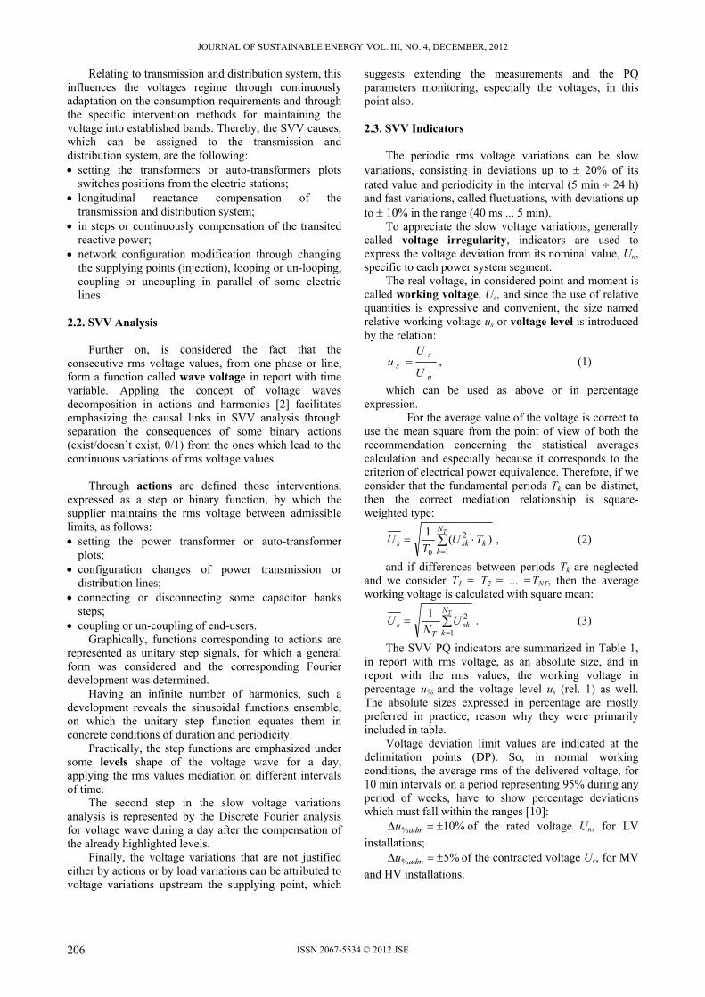
3.4. Highlighting levels in the voltage chart
To make more visible the possible levels from the
voltage variations chart the moving average was firstly represented of a range exceeding 10, adopting a half-hour (30) interval. The obtained graph, similar to one from Fig. 2, but with slower variations, has facilitated to emphasize the following four levels presented in Fig. 4: the first level with mean voltage Umed1=222,8 V,
recorded between 1010-1430, and having the working voltage VU s 7,225;7,220 ;
the second level with mean voltage Umed2=224,9 V, recorded between 1430-1700, and having the working
208
JOURNAL OF SUSTAINABLE ENERGY VOL. III, NO. 4, DECEMBER, 2012
ISSN 2067-5534 © 2012 JSE
voltage VU s 2,226;3,223 ;
the third level with mean voltage Umed3=222,8 V, recorded between 1700-2140, and having the working voltage VU s 6,226;2,220 ;
the 4th level with mean voltage Umed4=229,2 V, recorded between 2140-410, and having the working voltage VU s 3,232;5,221 ;
the 5th level with mean voltage Umed5=227,8 V, recorded between 410-600, and having the working voltage VU s 8,228;5,224 ;
the last level with mean voltage Umed6=223,8 V, recorded between 600-1010, and having the working voltage VU s 8,227;6,218 .
Even without detailing every single level, can be noticed some particularities on the complete representation of the voltage wave (Fig. 2). So, relating to the first level, can be observed that at the beginning, around 1100 am, there is clearly manifested the up-step plot position switching of the supplying transformer and after about 20 min its revenue, action highlighted by the TD diagram as well.(Fig. 3), the average voltage jump at the increasing plot position is around 3 V. Otherwise, the rms voltage presents oscillation around the average value (of 222,8 V), with slow periodicities, of 3045 min and amplitudes of 0,30,4 V.
Fig. 4 - Proposed levels for voltage variations graph, on the one day observation period,
and the characteristic intervals. Remaining to more general appreciations about the
next levels can be made the following observations: the second and the 5th levels are just “calm” like the
first one after that double plot commutation was passed;
the 3rd and the 4th levels reveal the continuous load decreasing on them periods.
the last level, more “disrupted”, presents the cumulative aspect of the load increasing with those relative frequent plots switching, through which the voltage maintaining system occurs automatically. The amounted effect of the load variation and of the plots and capacitor bank switching, lead to an inedited shape (“saw-tooth”), of the voltage wave, during on this last level period.
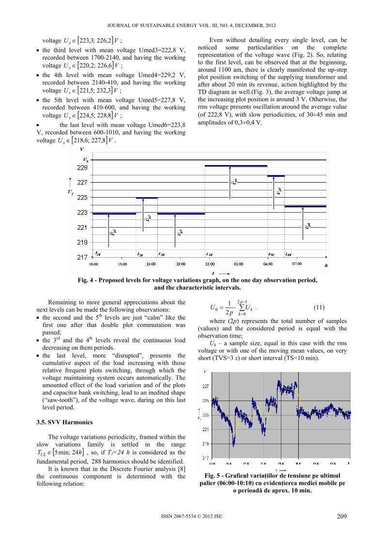
3.5. SVV Harmonics
The voltage variations periodicity, framed within the
slow variations family is settled in the range hTUL 24min;5 , so, if T1=24 h is considered as the
fundamental period, 288 harmonics should be identified. It is known that in the Discrete Fourier analysis [8]
the continuous component is determined with the following relation:
12
00 2
1 p
kkU
pU . (11)
where (2p) represents the total number of samples (values) and the considered period is equal with the observation time;
Uk – a sample size, equal in this case with the rms voltage or with one of the moving mean values, on very short (TVS=3 s) or short interval (TS=10 min).
Fig. 5 - Graficul variaţiilor de tensiune pe ultimul
palier (06:00-10:10) cu evidenţierea mediei mobile pe o perioadă de aprox. 10 min.
209

JOURNAL OF SUSTAINABLE ENERGY VOL. III, NO. 4, DECEMBER, 2012
ISSN 2067-5534 © 2012 JSE
Running the harmonic analysis program VI REGIDE for the last level emphasized in the voltage variation wave, given more detailed in Figure 5, led to the results shown in Table 2.
ERR=0,05 was introduced in the program as a relative error so that all harmonics with amplitudes in the error range are neglected. For the analyzed observation period (of 250 min) the 5 min limit periodicity corresponds to the 50th order harmonic. Therefore, all identified harmonics with a higher order than 50 are in the voltage fluctuations range and are not included in the table.
Among these, the following eight harmonics have the most important weights:
15,13,11,10,8,4,2,1impk ,
highlighting the network manifestation of some consumption characteristics with following periodicities:
min250,125,63,31,25,23,19,17kT .
Is can be noted that the most important slow voltage variation is quite the fundamental with 250 min periodicity while among slow variations with lower periodicity, the 34th order harmonic has a significant weight with a 7,4 min periodicity.
The SVV harmonics amplitudes, from the last level, are found in the following range:
VUk 33,13,0 .
Table 2. Voltage varations harmonics coresponding to the 6th level
k Uk, V
k Uk, V k Uk, V k Uk, V
0 0,108 9 0,323 19 0,123 33 0,159 1 1,325 10 0,520 20 0,247 34 0,229 2 1,310 11 0,523 23 0,157 36 0,130 3 0,613 12 0,197 24 0,290 37 0,096 4 0,893 13 0,346 25 0,237 38 0,098 5 0,271 14 0,194 26 0,164 40 0,168 6 0,276 15 0,301 27 0,235 41 0,158 7 0,234 17 0,280 29 0,119 42 0,114 8 0,428 18 0,274 31 0,120 50 0,134
A very important observation emerges from slow
voltage variations analysis that is the highlighted harmonic amplitudes do not monotonically decrease with their order which is visible from the third to 4th harmonic transition, from 7th to 8th etc.
The analysis of end-users processes would be able to reveal actions with the emphasized periodicities which were significantly manifested in SVV.
5. CONCLUSION
Applying the relative recent proposed methodology of decomposition the voltage wave in actions and harmonics, through the SVV identification, new aspects were emphasized in this application, such as “saw-tooth” variation profile. These aspects result through the effects of some continuous processes overlap, such as load variation, with some step type ones, where the actions like transformers plots and capacitor banks steps switching, are framed.
Comparing the decomposed voltage wave in levels, based on moving average, with the afferent actions
diagram on the distribution system elements, a good correlation between them was observed. In consequence, when an actions diagram is disposed, it must be placed on the levels defining base from the voltage wave.
In the measurement point of interest, the voltage average is lower with about 2,1% than the rated value, but the deviations are within admissible limits. The average deviation reduction toward zero may be a voltage control objective for this consumption point.
The emphasized levels in the analyzed voltage wave on one day have mostly a good justification through the variation form and through the power consumption evolution as well. It can be affirmed that the realized analysis in this application claims the decomposition methodology of the voltage wave in actions and harmonics, for emphasizing the SVV.
The experimental methodology, interlock to SVV analysis, must be developed through monitoring some points upstream the point of interest and also through the participation of all factors which occur through actions in transmission and distribution system. REFERENCES [1]. *** Technical quality analysis of voltage wave. Case
Study Distribution LES Baia Mare 4 - PA 7- PT Dieter, Baia Mare. Scientific Research Contract U.T.C.-N., nr. 33788/27.12.2010.
[2]. Maier, V., Pavel, S. G., Leşe, D. şi Beleiu, H.G. Fundamentals of Slow Voltage Variations Analysis. In: Proceedings of the international Conference OPTIM 2012, Braşov, Romania.
[3]. Buta, A. ş.a. Power Quality, „Electrical Engineering” Series. Bucureşti: Editura AGIR, 2001.Dugan, R.C. ş.a. Electrical Power Systems Quality. New York: McGraw Hill Companies, 2003.
[4]. Golovanov, Carmen ş.a. Modern Measurement Problems in Electrical Power System. Bucureşti: Editura Tehnică, 2001.
[5]. Iordache, Mihaela şi Conecini, I. Power Quality. Bucureşti: Editura Tehnică, 1997.
[6]. Maier, V. şi Maier, C.D. LabVIEW in Power Quality, Second Edition, completed. Cluj-Napoca: Editura Albastră, 2000.
[7]. Maier, V., Pavel, S. G. şi Maier, C. D. Power Quality and Environment Protection. Cluj-Napoca: Editura U. T. PRESS, 2007.
[8]. PE 143/2001 Normative for harmonics and unsymmetrical regime limitation in the electrical networks. Bucureşti, ISPE, 2001.
[9]. ***Performance Standard for Electricity Distribution Service, Cod ANRE 28.1.013.0.00.30.08.2007. Bucureşti, ANRE, 2007.
[10]. Maier, V., Maier, C.D. şi Miholca, Mihaela .L., Complete Virtual Instrument for Harmonics. In: "Virtual Instrumentation Magazine", 3(15)/2001, Cluj-Napoca. p. 71-79.
[11]. Maier, V. ş.a. Power Quality Control in Low and Medium Voltage Distribution Networks. În: Energetica, nr.1, ianuarie 2003.
[12]. Maier, V., Pavel, S. G. şi Maier, C. D. Power Quality Monitoring with Virtual Instruments. În: Energetica, anul 57, nr.4, aprilie 2009, pp. 214-219.
[13]. The Measurement and Automation Catalogue 2000, National Instruments, Austin, USA.
210

JOURNAL OF SUSTAINABLE ENERGY VOL. III, NO. 4, DECEMBER, 2012
ISSN 2067-5534 © 2012 JSE
SENSITIVITY ANALYSIS OF RELIABILITY FOR A TYPE STRUCTURE OF THE ELECTRICAL
DISTRIBUTION STATION
SECUI D.C., BENDEA G. University of Oradea, Universităţii no.1, Oradea,
Abstract – This paper presents a sensitivity analysis of reliability for an electrical distribution station of high voltage/medium voltage with a double busbars system. Sensitivity analysis is performed by evaluating two reliability indicators: number of interruptions and duration of interruptions, for a consumer connected to medium voltage busbars of the electrical station. In the final part a case study is presented, followed by concluding remarks. Keywords: reliability, electrical distribution stations, sensitivity analysis. 1. INTRODUCTION
Electrical distribution stations (EDS) are important structures in power systems that are designed to receive and convert the electricity supply and distribute required energy to feeders. EDS reliability study is of interest both from the point of view of the electricity company, and consumers. The failure of a component of the EDS results in loss of power to some of the consumers or to all consumers connected to the medium voltage (MV) busbar of EDS, causing their damage and high costs of electricity companies.
EDS reliability is evaluated through a set of indicators such as [1]: the probability of success and the probability of failure, the total duration of function and the total duration of failure, number of forced supply interruptions in consumers, energy not supplied to consumers, average power disconnected, equivalent failure rate, equivalent repair rate. In practice, two of these indicators are important, namely the number of interruptions and duration of interruptions at consumers.
Over time, several methods have been applied to study the reliability EDS: Markov chain method [2, 3], minimal cut set approach [4, 5], Monte Carlo simulation method [6-8], fuzzy approach [3, 9] or the approach based on failure mode and effect analysis [10, 11].
In [10] it is presented a methodology for assessing the reliability of high voltage transmission station with hierarchy structure components relative to various performance criteria of station (frequency and duration indices). In [12] power station reliability evaluation is performed using various criteria analysis.
To establish the contingencies before and after switching actions in [13] simulation algorithms are presented to evaluate the corresponding reliability indicators. 2. ANALYSIS METHOD
In this paper the EDS reliability analysis is reduced to the assessment of two main reliability indicators: number of interruptions (νC(TA)) and duration of interruptions (βC (TA)) at an equivalent consumer C, for a period of analysis (TA). Consumer C represents all consumers connected to a feeder connected to the medium voltage busbars of the analyzed EDS. The reliability analysis of the electrical distribution stations is performed using minimal cut sets technique [1, 14]. A minimal cut is composed of an element or several elements whose failure leads to the power interruption of the consumer.
The analysis considered only first and second order minimal cut set, their higher order cuts being neglected. Minimal cut set is done by visual research of the analyzed EDS configuration.
Given the failure modes of the EDS, we consider the following categories of events leading to interruption of the consumer C [1]: first-order total events (TEI), second-order total events (TEII), first-order active events (AEI), first-order active events overlapping stuck-breaker under condition opening (AES).
Notion of passive failure, active failure and total failure, and also their mathematical relations are presented in [1]. Their brief description is made below.
An active failure in a component requires the operation of the protection system near its, action that causes taking out of use of the damage component and possibly of other components. The component that has suffered an active failure is isolated and then removed into repair state. Part of affected consumers can be resupplied using other ways, through successful closing of breakers. Resupplying takes place after a while, called average switching time (which is less than the time needed to repair the damage component). A passive failure in a component does not require the operation of the protection system, and does not affect other components. The component that has suffered a passive failure is isolated and then removed into repair
211

JOURNAL OF SUSTAINABLE ENERGY VOL. III, NO. 4, DECEMBER, 2012
ISSN 2067-5534 © 2012 JSE
state. Following this type of failure the consumer could be
affected if the failure forms a minimal cut of a certain order. A total failure in one component comprises both types of mentioned failures (active and passive failure). Each of the mentioned failures can be characterized by two basic indicators: active failure rate (a) and average time repair (r) – for active failures; total failure rate (t) and average time repair (r) - for total failures. Average time repair (r) was considered the same for all failure types [1]. These indicators are used as input data in EDS analysis.
In case of supply interruption at the consumer C, first-order total events (TEI) and first-order active events (AEI) involve the failure of a single element i. Total failures are considered by the total failure rate (t
i) and active failures are considered by active failure rate (a
i) of the element i. After a first-order total events (TEI) at the element i,
the consumer is resupplied after a duration corresponding to the average repair time (ri). After a first-order active events (AEI) at the element i, the consumer is resupplied after a duration corresponding to the average switching time (tc).
Second-order total events (TEII) implies the failure of two elements i and j. Equating the two elements i and j is done using the relations [1, 14]:
jtji
ti
jitj
tit
)j,i(rr1
)rr(
(1)
ji
jit)j,i( rr
rrr
(2)
where, ti, t
j represents total failure rate for the element i, respectively j; ri, rj are the average repair time for the element i, respectively j.
AES events imply an active failure of an element i overlapping with stuck-breaker who must protect the element i. The average interruption time of the consumer is equal the average switching time (tc), which is considered known. The failure rate (i
Stuck) specific to the event is determined with the relation [1]:
bai
Stucki P (3)
The main steps for the evaluation of the reliability indicators (νC(TA), βC(TA)) at the consumer C are: 1. for each element of the EDS (breakers, disconnectors, power transformers, busbars etc), the reliability indicators (a, t, r) are identified based on norms; also the average switching time (tc) and the probability of stuck-breaker (Pb) are determined; 2. minimal cuts identification of I and/or II for each of the events considered (TEI, TEII, AEI and AES); 3. determination of equivalent reliability indicators for each element or pair of elements that form a particular category of events: for each element i of TEI category is determined the pair of indicators (t
i, ri); for each element i of AEI category is determined the
pair of indicators (ai, tc);
for each pair of elements (i,j) of TEII category is determined the pair of indicators (t
(i,j), rt(i,j)) using the
relations (1) and (2); for each element i of AES category is determined the pair of indicators (i
Stuck, tc) using the relation (3).
4. for the events categories (TEI, TEII, AEI and AES) is determined the pair of indicators (equivalent failure rate, average time of consumer C resupplying) using the series type relations (events from each category are in series with the consumer); 5. Grouping categories of events: events which determine interruptions of duration (ID), respectively events which determine interruptions short duration (IS) at consumer C. The ID interruptions include events TEI and TEII, and IS interruptions include events AEI and AES; 6. for each type of interruption (ID and IS) is determined the pair of indicators (ID, rID) and (IM, rIM), where ID, IM represents equivalent failure rate for ID interruptions, respectively IS interruptions; rID, rIM are the equivalent average repair time corresponding to ID and IS interruptions. (ID, rID) and (IM, rIM) indicators are determined using the series type relationship (4) - (7):
III DTDTID (4)
ID
DTDTDTDTID
IIIIIIrr
r
(5)
SI DADAIM (6)
cIM tr (7)
where, DTI, DTII, DAI, DAS represent equivalent failure rate corresponding to DTI, DTII, DAI and DAS events; rDTI, rDTII are equivalent average repair time corresponding to TEI, respectively TEII events; 7. determining synthetic reliability indicators for consumer C (νC, βC) considering both the ID interruptions effect, as IS interruptions effect. The calculation is performed considering the two series events (ID and IS). EDS reliability analysis is performed considering these assumptions:
- for each equipment both failure time and repair time have exponential distributions;
- the reliability of equipments and power lines that feed EDS system is not taken into account;
- the influence of weather on EDS and the influence of preventive maintenance strategies is not considered;
- each feeder connected to the medium voltage EDS busbars is represented by an equivalent element E;
- the equipments of the same type and the equipments functioning at the same voltage level have the same primary reliability indicators;
- the probability of failures of higher order than three is neglected;
212
JOURNAL OF SUSTAINABLE ENERGY VOL. III, NO. 4, DECEMBER, 2012
ISSN 2067-5534 © 2012 JSE
3. SENSITIVITY ANALYSIS
The sensitivity analysis studies the output parameters variation in relation to the variation of the input parameters for a model. In this paper, the output parameters are the number of interruptions ID (νID) and the number of interruptions IS (νIS) for the consumer, as the duration of interruptions ID (βID), and respectively IS (βIS), for the consumer. The input parameters which are varied in this paper are: the total failure rate (t
i) and the active failure rate (a
i) for the equipment i from EDS structure.
Sensitivity analysis has in view two groups of equipments. The first group (group 1) consists of equipments of the same type, such as all disconnectors of MV or HV, all breakers of MV or HV etc. The second group (group 2) includes all equipments with the same voltage level. In this category will include: all equipments of the medium voltage, all the equipments of high voltage and the power transformers of HV/MV.
For analyzing the sensitivity of indicators (νID, νIS, βID and βIS) the following methodology was applied: 1. EDS reliability is assessed (using the algorithm presented in Section 2) for the initial case (α=0). Thus, the set of indicators (νID(0), νIS(0), βID(0) and βIS(0)) is determined at the C consumer; 2. the total failure rate is reduced by the same percentage α (t
i← (1-α)ti) for a type of equipment i from EDS
structure (group 1) or for all the equipments of the same voltage level (for group 2). Average repair time ri, average switching time tc and the probability of stuck-breaker Pb are maintained fixed; 3. EDS reliability is reassessed using the algorithm in Section 2, and the following set of indicators (νID(α), νIS(α),
βID(α) and βIS(α)) is obtained; 4. it is calculated the relative reduction (ΔI) of the reliability indicators due to the t
i rate reduction by the percentage α, for the equipment i (group 1, respectively group 2):
ΔI=(I(0)-I(α))·100/I(0) (8)
where I(0), I(α) represents a certain indicator (νID, νIS, βID, βIS) assessed for the initial case (α=0), respectively for a percent α0; 5. it is identified the set of the equipments which is the most sensitive to the changes of the total failure rate t
i; 6. indicator I(α) variation it is graphic represented considering α percentage values within the range [0,100]. 4. CASE STUDY
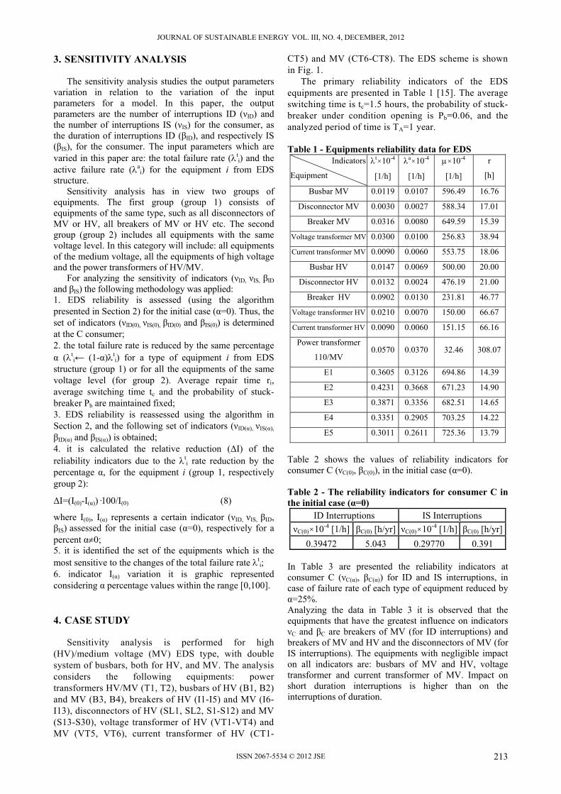
Sensitivity analysis is performed for high (HV)/medium voltage (MV) EDS type, with double system of busbars, both for HV, and MV. The analysis considers the following equipments: power transformers HV/MV (T1, T2), busbars of HV (B1, B2) and MV (B3, B4), breakers of HV (I1-I5) and MV (I6-I13), disconnectors of HV (SL1, SL2, S1-S12) and MV (S13-S30), voltage transformer of HV (VT1-VT4) and MV (VT5, VT6), current transformer of HV (CT1-
CT5) and MV (CT6-CT8). The EDS scheme is shown in Fig. 1.
The primary reliability indicators of the EDS equipments are presented in Table 1 [15]. The average switching time is tc=1.5 hours, the probability of stuck-breaker under condition opening is Pb=0.06, and the analyzed period of time is TA=1 year. Table 1 - Equipments reliability data for EDS Indicators
Equipment
t×10-4
[1/h]
a×10-4
[1/h]
×10-4
[1/h]
r
[h]
Busbar MV 0.0119 0.0107 596.49 16.76
Disconnector MV 0.0030 0.0027 588.34 17.01
Breaker MV 0.0316 0.0080 649.59 15.39
Voltage transformer MV 0.0300 0.0100 256.83 38.94
Current transformer MV 0.0090 0.0060 553.75 18.06
Busbar HV 0.0147 0.0069 500.00 20.00
Disconnector HV 0.0132 0.0024 476.19 21.00
Breaker HV 0.0902 0.0130 231.81 46.77
Voltage transformer HV 0.0210 0.0070 150.00 66.67
Current transformer HV 0.0090 0.0060 151.15 66.16
Power transformer
110/MV 0.0570 0.0370 32.46 308.07
E1 0.3605 0.3126 694.86 14.39
E2 0.4231 0.3668 671.23 14.90
E3 0.3871 0.3356 682.51 14.65
E4 0.3351 0.2905 703.25 14.22
E5 0.3011 0.2611 725.36 13.79
Table 2 shows the values of reliability indicators for consumer C (νC(0), βC(0)), in the initial case (α=0). Table 2 - The reliability indicators for consumer C in the initial case (α=0)
ID Interruptions IS Interruptions
νC(0)×10-4 [1/h] βC(0) [h/yr] νC(0)×10-4 [1/h] βC(0) [h/yr]
0.39472 5.043 0.29770 0.391 In Table 3 are presented the reliability indicators at consumer C (νC(α), βC(α)) for ID and IS interruptions, in case of failure rate of each type of equipment reduced by α=25%. Analyzing the data in Table 3 it is observed that the equipments that have the greatest influence on indicators νC and βC are breakers of MV (for ID interruptions) and breakers of MV and HV and the disconnectors of MV (for IS interruptions). The equipments with negligible impact on all indicators are: busbars of MV and HV, voltage transformer and current transformer of MV. Impact on short duration interruptions is higher than on the interruptions of duration.
213
JOURNAL OF SUSTAINABLE ENERGY VOL. III, NO. 4, DECEMBER, 2012
ISSN 2067-5534 © 2012 JSE
Fig. 1 - The analyzed EDS
Table 4 shows the results for the case in which the sensitivity analysis is performed for the equipments located at the same voltage level. Table 3 - The impact on reliability indicators for consumer C (group 1)
ID Interruptions IS Interruptions Indicators Equipment
νC(α)×10-4 [1/h]
βC(α) [h/yr]
νC(α)×10-4 [1/h]
βC(α) [h/yr]
Breaker MV 0.38678 4.936 0.28470 0.374
Disconnector MV 0.39434 5.038 0.28656 0.377 Voltage transformer MV
0.39472 5.043 0.29520 0.388
Current transformer MV
0.39471 5.043 0.29734 0.391
Busbar MV 0.39472 5.043 0.295025 0.388
Breaker HV 0.39453 5.038 0.28307 0.372
Disconnector HV 0.39470 5.043 0.29283 0.385
Voltage transformer HV
0.39471 5.043 0.29574 0.389
Current transformer HV
0.39470 5.042 0.29716 0.390
Busbar HV 0.39472 5.043 0.29597 0.389
Power transformer 0.39450 5.027 0.29548 0.388
Following the results of Table 5 it is noticed that the MV equipments have a greater impact than those of HV, on the indicators νC and βC. Also, IS interruptions are changing more than ID interruptions. The relative reduction of the indicators νC and βC, in case of IS interruptions, is the same because the average switching time (tc) is the same for any resupplying operation of the C consumer.
Table 4 - The impact on reliability indicators for consumer C (group 2)
ID interuptions IS interuptions Indicators Equipment
νC(α)×10-4 [1/h]
βC(α) [h/yr]
νC(α)×10-4
[1/h] βC(α)
[h/yr]
All MV equipments 0.38639 4.930 0.26803 0.352All HV equipments 0.39447 5.037 0.27398 0.360
Power transformer 0.39450 5.027 0.29548 0.388
Table 5 - The relative reduction (ΔI, I={ν,β}) of reliability indicators for consumer C (group 2)
ID interuptions IS interuptions Indicators Equipment
ΔνC(α) [%]
ΔβC(α) [%]
ΔνC(α) [%]
ΔβC(α) [%]
All MV equipments -2.110 -2.236 -9.967 -9.967All HV equipments -0.063 -0.129 -7.968 -7.968
Power transformer -0.057 -0.318 -0.746 -0.746
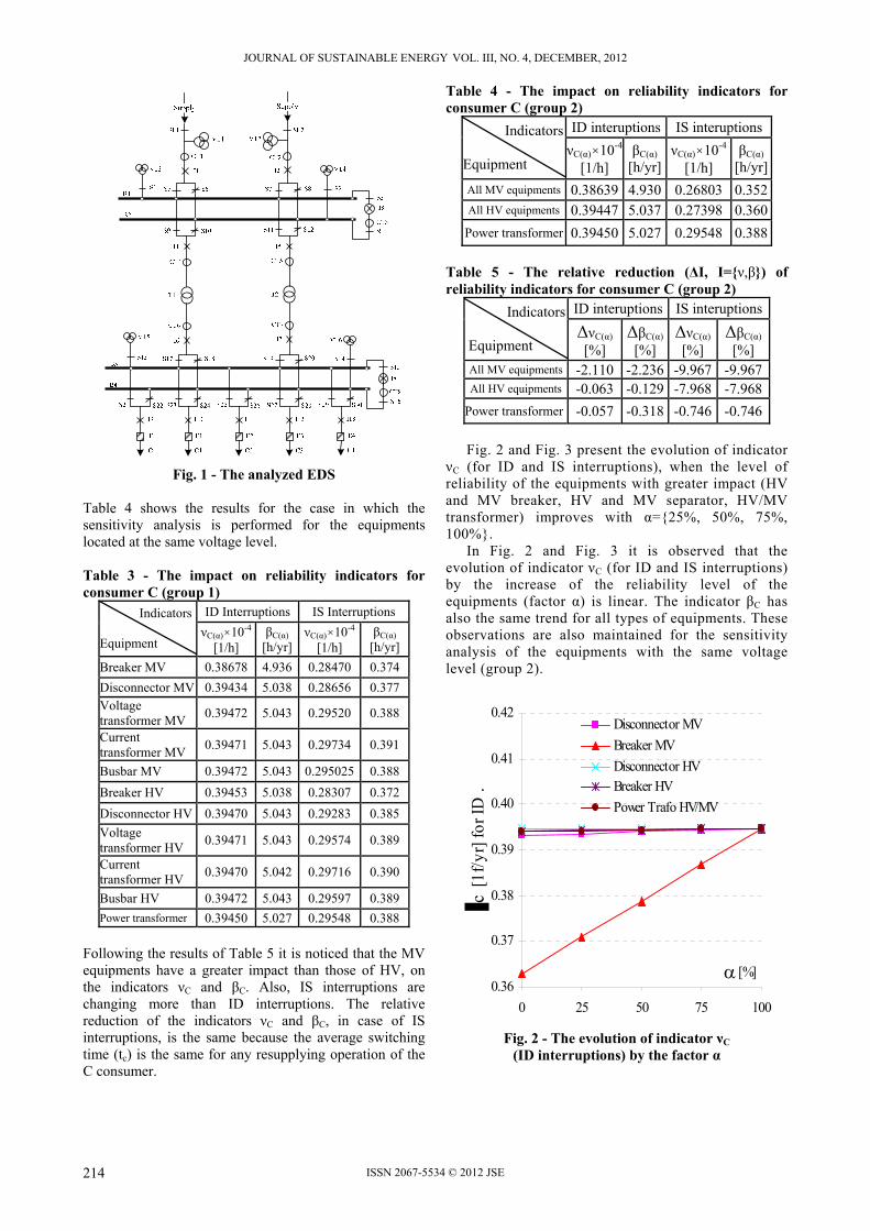
Fig. 2 and Fig. 3 present the evolution of indicator
νC (for ID and IS interruptions), when the level of reliability of the equipments with greater impact (HV and MV breaker, HV and MV separator, HV/MV transformer) improves with α={25%, 50%, 75%, 100%}.
In Fig. 2 and Fig. 3 it is observed that the evolution of indicator νC (for ID and IS interruptions) by the increase of the reliability level of the equipments (factor α) is linear. The indicator βC has also the same trend for all types of equipments. These observations are also maintained for the sensitivity analysis of the equipments with the same voltage level (group 2).
0.36
0.37
0.38
0.39
0.40
0.41
0.42
0 25 50 75 100
[%]
c [1
f/yr
] for
ID
.
Disconnector MV
Breaker MV
Disconnector HVBreaker HV
Power Trafo HV/MV
Fig. 2 - The evolution of indicator νC
(ID interruptions) by the factor α
214
JOURNAL OF SUSTAINABLE ENERGY, VOL. III, NO. 4, DECEMBER, 2012
ISSN 2067-5534 © 2012 JSE
PRINCIPLES OF EVALUATION OF RELIABILITY OF THE EQUIPMENT OF THE POWER
ELECTRICAL DISTRIBUTION SYSTEMS
LUKYANENKO E. Academy of Sciences of Moldova
Abstract. The Power electric distribution systems (PEDS) possess a great dynamics of development. Thanks to this phenomenon in the power electric distribution systems (PEDS) the probability of apparatus of asymmetrical regimes increase monotonously. As a result of this reliability of the functioning of the power electric equipment installed in the electric knots changes. The asymmetrical regimes in the power electric distribution systems (PEDS) accompanied by the short circuit current are a function of a row determinate is a vague factor of probabilistic nature. Coming from it follows that the investigation of the influence of the asymmetrical regimes accompanied by the current of the short circuit on the reliability of the power electric distribution systems (PEDS) is one of the most important problems of the development the power electric distribution systems The short circuit currents influence the structural and functional reliability of distribution networks and at the reliability of electrical equipment installation
Keywords- Power electric distribution systems reliability of electrotehnical equipment, asymmetrical regimen, accompanied, current of the short circuit 1. INTRODUCTION
Power systems and power distribution have a pretty dynamic development highlighted.
This phenomenon is due to more extensive use of electricity in various branches of national industry (industry, agriculture, and social sector), etc. Following the installed generating nodes and continuously growing system entirely.
The electrical distribution systems monotonically increasing continuously and discretely short-circuit current (SC), which brings to the variation of operating reliability of equipment and electrical equipment installed in knots.
This paper is the study and analysis of the influence of short circuit currents on equipment reliability and electrical equipment installed at bus power distribution systems.
2. MATERIALS AND METHODS
Power equipment reliability problems are some of the most pressing issues of forecasting and of operating the electric power industry and depend on a number of factors so determined and undetermined.
Therefore this problem requires special attention. Known methods of analysis and evaluation of reliability indices (both of networks, nodes and electrical equipment and the systems of power and distribution in full), in some cases do not meet these requirements because it does not take into account all factors that influence the reliability of equipment and electrical machinery.
Short circuit currents power electrical systems probabilistic in nature and takes on values determined at different stages, which depend so installed as well as the state power and the electrical components to short-circuit timing. Therefore the study and research of the influence current values of sc the reliability of networks, nodes and electrical equipment installed in power systems is one of the most pressing issues on power systems and power engineering development in full.
To determine the influence of an electric power system was studied for 25 years every 5 years. In each period were calculated values of short circuit current and expected level of reliability.
Analysis of the results gained indicates that node reliability as the reliability of distribution systems components, wiring diagrams in the systems of nodes and the expected values of short circuit currents.
Dependence was established reliability elements and transport nodes mainframe systems and power distribution depending on the short circuit current values )I(fR SC .
In the process of calculating and assessing the reliability of elements and nodes mainframe systems of electricity transmission and distribution was determined that short-circuit currents have a primary influence on the reliability of equipment. It was found that the status of these elements depends not only reliable nodes as they are installed, but a large part of the mainframe systems reliability of electricity transmission and distribution connected with given node. Analysis of operating the equipment indicates that reliability depends on the following factors:
a) expected values of the short circuit currents which may occur in the system; b) frequency of occurrence of short circuit currents;
215
JOURNAL OF SUSTAINABLE ENERGY, VOL. III, NO. 4, DECEMBER, 2012
ISSN 2067-5534 © 2012 JSE
c) transient recovery voltage )(tUTR that appears
to breaker bars, and their variation. Reliability of operation of circuit breakers and
disconnect their ability is directly proportional to the cube of short circuit current given node. Ability to disconnect switches any circuit is characterized by exchange rate (variation of electricity derived from short circuit breaker bars [1,2].
If the variation of electric short circuit current limit is msc/A,10dt/di2 sc , the probability and during
the occurrence of arcing across the breaker is minimal and when this switch can disconnect any circuit.
If electric short circuit current variation is within, msc/A,30dt/di15 sc , then disconnect any
type of air circuit breakers is defensible by any type of switch that is currently in operation, the system studied.
Depending on the expected values of the short circuit currents, moving to short circuit breaker, disconnect the short circuit is characterized by short circuit disconnection factor complicity. These factors characterize the influence of different parameters on the operation of circuit breakers now.
As parameters are: a) the maximum expected short circuit currents of disconnection; b) amplitude and current variance component a periodic short circuit; c) first derivative amplitude initial period of transient recovery voltage circuit breakers to bars on both sides; d) dynamic forces acting on breaker bars; e) ambient temperature, arc length and other factors that may have direct influence.
The value of this factor depending on the values of short circuit current and maximum current disconnect to disconnect the circuit breaker is determined by the expression:
)t(CLIK )3(SCt (1)
where: C-is coefficient of proportionality, C = 0.375; L - distance where the short circuit occurs to the bar;
)()3( tI SC -the value of three-phase short circuit current.
)1(SCI -the current single-phase short circuit
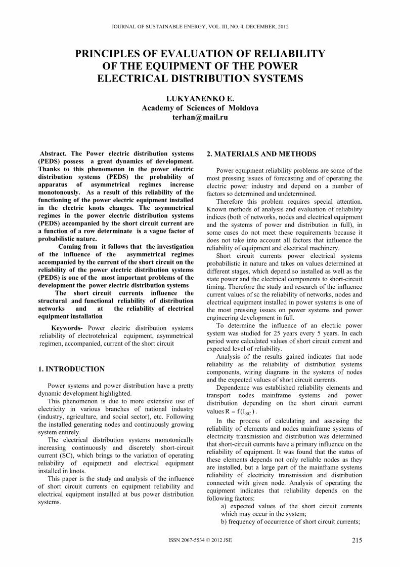
The analysis results of, the network system reliability and system reliability of the equipment installed in the nodes depend on dynamic changes of sc currents. Reliability of the expected dependence of short circuit currents are shown in fig. 1
8.76.14
8.19
5.23
CUR .0.1
993.0
2000 2005 2010 201585.09.00.1
)(3 kAISC
T
Fig.1 - The dependence on the reliability of random
values of short circuit currents One of the parameters that characterize the reliability
of circuit breakers is the flow of refusal [ω (t)]. To assess flow refusal developed a mathematical model which enables to take into account the number of cycles and intensity of operation since last overhaul. In this case the frequency of operation without refusal )t( is
determined as [3] depending on the values )t(I )1(SC ;
)t(I )3(SC .
If the frequency of operation 1 the commissioning
of the equipment 2 and time of taking the overhaul are
known then the limit of the operation in terms of reliability can be determined by the expression:
)t(e)t(p (2)
where: )(tp - is it possible to decrease the
probability limit of operation until the next repair of equipment;
)( 21 - the difference in probability at
the beginning and end of the operation. The number of complete cycles depending on the likelihood and frequency of operation is determined by the expression:
)t(0eN)t(N (3)
where: No - is the number of cycles of operation of the circuit breaker that disconnects currents. value less than 10% of the maximum expected under STAS 687-89. The breaker reliability )t(R the number of cycles until
the next revisions to the repair or removal of )t(N by the
currents of short circuit disconnect wait. The short circuit current SCI was determined experimentally and
presented in table 1.
216

JOURNAL OF SUSTAINABLE ENERGY, VOL. III, NO. 4, DECEMBER, 2012
ISSN 2067-5534 © 2012 JSE
Table 1.
)(
)()3(
)1(
tItI
SCN
SC
0.08 0.16 0.25 0.50 0.75 1.00
N(t) 32 26 20 15 12 10 R(t) 0.9998 0.9997 0.9996 0.9996 0.9993 0.9991
where: N (t) - is the number of cycles performed by switch disconnects; R (t) - is reliability of operation of circuit breakers.
In considering the influence of short circuit currents on fiability necessary to take into account not only the expected values of short circuit currents, but also the thermo effect, they produce this year. The influence of thermal effect of the short circuit currents in this case is determined by thermal pulses, which are proportional to the square values of short circuit currents and can be determined from the following expression:
dttZtItWk )()()( 2 (4)
where: )(2 tI - is the effective value of short circuit
disconnected. From the above it is clear that reliability of operation of circuit breakers is a multifactor function determined by the currents of short circuit, transient change in voltage, short circuit factor aiding the disconnected [3,4]. In the analysis all relationships determined duration and frequency is received that has a probability distribution (p = 0.9997) and follow laws, corresponding Waybill distribution. In this case this function can be determined from (5).
Tt
eT
ttf)1()(
)(
( t > 0 ) (5)
where: T is the period of operation, t-the emergence of refusal set; 0 - shape the distribution of refusals. The probability to refuse equipment operating in conditions that do not meet technical requirements (because that increases the probability of rejection) of all equipment can be determined from expression (6).
btAbR aKKatp )1()( 0 (6) where: ab - is automatic recouping index (ab= 1 if automatic recouping works without denial, ab = 0 if automatic recouping missing.) KA - coefficient taking into account the automatic recouping cycles without success;
Kt - coefficient of complicity to disconnect the short circuit real;
0ba - number of disconnects unsuccessful according to
the values of short circuit currents. Statistical analysis of materials (all refusals breakers) shows that about 25% of all refusals occur because of external insulation defects, therefore is necessary to introduce the correlation coefficient (kτ = 0.25), taking into account the decreasing reliability of due to external faults. In this case taking into account all described it can be concluded that the indicators and the reliability of circuit breakers is based on random values of short circuit currents. 3. CONCLUSIONS
1. Comprehensive analysis of equipment reliability
and electrical equipment installed in electricity distribution systems r EEA show that it depends on the expected values of short circuit currents, the transient recovery voltage and its variation in bars equipment and number of cycles performed. This feature bears a linear character.
2. Probability values of short circuit currents expected to meet technical requirements for electrical equipment reference. Otherwise it is necessary to develop additional measures to limit the short circuit current values of increase.
3. To determine the influence of short circuit current and voltage transient on indicators of reliability of equipment and machinery in distribution systems has developed a mathematical model that takes into account the dynamics of change of short circuit currents.
BIBLIOGRAPHY
[1]. Ragaller K. Otklûcenie tokov v seteah vysokogo napryaženiâ. M: Ènergoatomizdat, 1981 -327 s.
[2]. Erhan F., Neklepaev B. Toki korotkogo zamikaniâ i nadežnosti energosystem; M.: Energoatomizdat, 1987 – 345 s.
[3]. Neklepaev B.N. Koordonaciâ i optimizaciâ urovnei tokov korotkogo zamikaniâ v electroenergheticeskih sistemah. M; Ènerghiâ, 1978 - 167s.
[4]. Erhan T., Melnic S. Short-circuit current level effect on the electric power systems reliability. The III - Internasional Symposion " Short-circuit currents in power system" Polond, Sulejow 1988, V-I, 81-89 p.
217

JOURNAL OF SUSTAINABLE ENERGY VOL. III, NO. 4, DECEMBER, 2012
ISSN 2067-5534 © 2012 JSE
GROUND-MED PROJECT AT THE UNIVERSITY OF ORADEA
BENDEA C.*, ROSCA M.*, KARYTSAS K.**, BENDEA G.* *University of Oradea, Universităţii no.1, Oradea,
**Centre for Renewable Energy Sources, Athens, Greece, [email protected], [email protected], [email protected], [email protected]
Abstract: The paper presents an overview on ground source heat pumps technology, focusing then on Ground-Med project, describing its aim and objectives, partners involved, location of demo-sites and heat pump manufacturers. Then, the article presents the University of Oradea demo-site, showing the chosen building, describing its thermal characteristics and the technical solution which is used for space conditioning.
Key words: Ground coupled heat pump, Ground-Med project demo-site
1. INTRODUCTION
Ground source heat pumps (GSHP) are systems comprising: a) ground heat exchanger (pipes buried horizontally in trenches or vertically in boreholes, through which water is circulated as a heat carrier), b) water source heat pump,
c) low temperature heating (and cooling) system (fan-coils, slim pipes under the floor or on the walls, etc.). As they exploit the favorable heat transfer properties of water and the mild ground temperature, which remains almost constant throughout the year, independently of external weather conditions, ground source heat pumps provide efficient heating, cooling and domestic hot water supply to the buildings. In cooling mode, they use 30% less electricity than air source heat pumps of latest technology. In heating mode, currently available technology provides a seasonal performance factor (SPF) up to 4, which means that out of 4 units of thermal energy delivered, 3 units are free geothermal energy and only 1 unit is electric energy consumed by the heat pump, resulting in a 75% energy savings. As regarding primary energy, the scheme below illustrates how 1 unit of fuel energy is transformed to 2.36 units of useful heat by ground source heat pumps (Figure 1), indicating that GSHP can play a major role to rational use of energy and fighting climate change. This is being recognized more and more by European citizens, who adopt the technology in increasing numbers.
Fig. 1 - Primary energy converted to useful heat by GSHP
As they are a reliable and environmental friendly technology, they can be an effective aid to fulfill the targets for renewable energy use and CO2 emissions reduction. Geothermal energy is becoming all around Europe one of the most interesting sources of renewable energy for the future in the sense of heating and cooling by ground coupled heat pumps. Energy policy and climate protection are top issues as each head of state and government committed to a binding target for 20% renewables by 2020. However, although ground source heat pump technology and market are developed in Western European countries, the corresponding market in Romania is at early developing stage, despite the
fact that both economics and CO2 emissions reduction potential are favorable, due to prevailing climatic conditions and the need for cooling. The cooperation work program for Energy supports technology development and demonstration of ground source heat pumps aiming at increasing the coefficient of performance (COP) of the heat pump and of the overall system in order to reduce the electricity consumption and extend its use in Europe. The increase of efficiency will reduce operating costs and pay-back time. GROUND-MED is a collaborative project which demonstrates innovative ground source heat pump solutions in 8 buildings in Mediterranean EU member States. It involves 25% research and technology development and
218

JOURNAL OF SUSTAINABLE ENERGY VOL. III, NO. 4, DECEMBER, 2012
ISSN 2067-5534 © 2012 JSE
75% demonstration (including dissemination activities) of integrated GSHP systems for heating and cooling of considerably higher seasonal coefficient of performance (SPF) than present technology. 2. GROUND-MED PROJECT 2.1. Project objectives The main objective of GROUND-MED is to demonstrate the superior energy efficiency (SPF>5.0 for year round operation) of the next generation of ground source heat pump systems for heating and cooling in South Europe. For this purpose 8 building-demonstration sites have been selected (one in Portugal, two in Spain, one in South France, one in Italy, one in Slovenia, one in Romania and one in Greece). The global aim is to demonstrate integrated ground source heat pump systems of:
annual SPF for both heating and cooling higher than 5.0
less than 7 years payback time compared to a system comprising natural gas boiler of 0.04 �/kWh for heating and air source heat pumps of COP = 3.5 for cooling
high system durability expressed as at least 20 years life span.
The first statement has a straightforward direct impact on energy efficiency. The other two statements define whether the proposed technological solutions and practices will be widely accepted by the end users or not, and are essential conditions, if we aim at their wide market penetration and large scale impact. Demonstrating the superior performance of the technology is essential in order to facilitate its introduction on the market. In order to demonstrate ground source heat pump systems of measured SPF>5, which is an ambitious target, the following technological solutions or practices will be demonstrated and evaluated: Improve the energy efficiency of the heat pump
units during all year operation: for this purpose the next generation of heat pumps will be developed by further optimizing individual components and introducing energy efficiency improving technologies such as variable capacity compressors. In addition, collaboration will be established by the consortium with compressor manufacturers towards the development of new compressor technology matching high efficiency motors with superior isentropic efficiency. In particular, develop water source heat pumps of SPF>5 in both heating and cooling modes for operation with a ground heat exchanger (8°C water supply to the evaporator in winter and 25-30°C water supply to the condenser during summer) and produce 8 prototypes for all demo sites as follows: 3 prototypes of large capacity, 3 prototypes of medium capacity and 2 prototypes
of small capacity one of which will use natural fluids as refrigerant.
Reduce electricity consumption of key system components as follows: − Develop low energy fan-coil units for operation with water of low temperature (35°C) in heating mode; produce prototypes for 50-100 kW system. − Develop air handling units (AHUs) using condensing heat rather than electric resistors for heating the air during winter and removing humidity during summer; produce one prototype.
Reduce the capacity of the heat pump and the size of the ground heat exchanger, while improving the COP and reliability of the system by using cold and heat storage. For this purpose prototype nodules for low temperature heat storage (~40°C) will be developed, and the feasibility of the technology will be evaluated.
Develop system controls, in order to minimize the temperature difference the heat pump has to overcome in order to heat or cool the building which results in large improvement of system SPF. This can be achieved by: Control the water temperature delivered by the
ground heat exchanger according to the heating/cooling load.
Control the water supply temperature to the heating/cooling system according to the heating/cooling load, e.g. in heating operation the water supply temperature from the heat pump could be 40°C at peak load and only 30° at partial load, while during cooling operation it could vary from 8°C at peak load and 15°C at partial load.
Optimize the ground heat exchanger in terms of improving the overall system SPF, while keeping capital costs at acceptable levels. For this purpose, ground heat exchangers will be designed using water (no antifreeze) as circulating fluid and at least 8°C water supply to the evaporator in winter and 25-30°C water supply to the condenser during summer.
Optimize the water temperature the heat pump supplies to the heating/cooling system of the building, e.g. as low as possible temperature during heating and as high as possible temperature during cooling mode.
Design each demonstration heating/cooling system for maximum energy efficiency.
Integrate the automation of the heat pump, the pumps, and fans with the building energy management system and optimizing overall energy performance.
Develop a regular maintenance program for improving system reliability by developing standard operation and maintenance specifications and procedures for each system.
2.2. Consortium members The GROUND-MED consortium comprises 24 organizations, mainly from South Europe, but with participants from central and north EU member States as well. It includes a wide diversity of GSHP actors, such as major research and educational institutes (CRES, CEA, UOR, ISR, UPV, UCD, UNIPD, ESTSetubal, KTH), leading heat pump manufacturers (CIAT, HIREF, OCHSNER), the
219

JOURNAL OF SUSTAINABLE ENERGY VOL. III, NO. 4, DECEMBER, 2012
ISSN 2067-5534 © 2012 JSE
national and European industrial associations concerning heat pumps and geothermal energy (EHPA, EGEC, GRETh), leading consulting organizations in geothermal or renewable energy matters (GEJZIR, ECOSERVEIS, GROENH), specialized works contractors (GEOTEAM, EDRASIS), the European heat pumps testing, evaluation and certification centre of heat pumps (CETIAT) and a well known information centre (FIZ). The 8 demonstration sites are dispersed in a wide geographic area (Portugal, Spain, South France, Italy, Slovenia, Romania and Greece), in order to maximize project market impact.
Fig. 2 - GROUND-MED demo-site locations
For each one of the 8 demonstration sites, one partner, usually the building owner (CIAT, HIREF, UOR, ISR, UPV, EDRASIS) or having established partnership relation to the building owner (GEJZIR, ECOSERVEIS), has been appointed as responsible partner. In order to exploit the experience gained and research results from previous European projects GROUNDHIT (heat pump technology development and demonstration) and SHERPHA (heat pump technology development using natural refrigerants) the consortium includes 6 organizations involved in the GROUNDHIT project (CRES, CIAT, UOR, GEOTEAM, EGEC, ESTSetubal) plus 10 organizations from the SHERPHA project (EHPA, FIZ, HIREF, UPV, GRETh, UCD, UNIPD, CETIAT, GROENH and KTH). The Centre for Renewable Energy Sources and Savings - CRES, GROUND-MED coordinator, is an experienced coordinator of European projects and as the national coordination centre of Greece for renewable energy sources and energy saving has been actively involved in the coordination of many European and national technology development and demonstration projects on ground source heat pumps. The heat pump manufacturers involved in technology development tasks of GROUNDMED are CIAT, the manufacturer of the GROUNDHIT prototypes, HIREF, manufacturer of SHERPHA natural fluid prototypes and OCHSNER as a heat pump manufacturer of central Europe where the corresponding technology is well developed, and in particular of Austria, where GSHPs have a leading market position.
3. INNOVATIVE TECHNIQUES Until now, heat pump research activities focused on COP improvements. GROUND-MED will advance the technology one step further from GROUNDHIT prototypes of COP>5.5 at nominal conditions by focusing on SPF. For this purpose, and considering that ground source heat pumps operate most of the time at much different conditions than the nominal ones, apart from improving heat pump units in terms of COP, technologies resulting in higher SPF will be considered. Present ground source heat pumps have ON-OFF modulation and are usually designed for use with fan-coils at 40/45°C, or 50°C condensing temperature, which is the set point for covering heating peak loads. This means that the COP of the heat pump will be 3.5 in all conditions, and the corresponding SPF somewhat lower due to high starting current, electricity consumption during stand-by periods and auxiliary power consumed by the water circulating pumps, the fan-coils and the air handling units. In many cases however, radiators are used instead of fan-coils, which results in even higher condensing temperatures and even lower efficiency. The heat pumps developed for the GROUND-MED project will be able to modulate the condensing temperature according to the heating load requirements, so that their COP will be maintained above 5.0 most of the time. Furthermore, the set point that corresponds to maximum heat load, will be reduced to less than 40°C, by developing a specially designed fan-coil that can operate at low temperature with 30% less electricity consumption (present fan coils are designed for temperatures higher than 45°C and their operation at lower temperatures is costly in terms of electricity consumption). The operation of the heat pump in cooling mode during summer will be improved accordingly, by setting the heat pump for operation delivering cold water between 15/10°C and 25/20°C, compared with 12/7°C of present systems. Furthermore, the operating conditions within the borehole heat exchanger (water flow rate and temperature range) will be optimized based on the above concept, aiming in maximizing the overall system SPF, defined as the useful heat and cold delivered by the GSHP over the sum of electricity consumption at the heat pump, the water pumps, the fans of the fan-coils, and the air handling unit. In order to obtain operation at the above discussed conditions, innovative ground source heat pump systems will be developed and demonstrated integrating the following technologies / solutions: Advanced water source heat pumps of high efficiency: Capacity modulation New generation of compressors matching motors of
high efficiency with superior isentropic efficiency Innovative heat exchangers for high efficient
cooling as well as heating Use of natural refrigerants in one prototype
Innovative system controls integrating all components (BHE pump, heat pump, water distribution pump, fans);
Smooth system start-up; Advanced fan-coils: low temperature operation in heating mode,
220

JOURNAL OF SUSTAINABLE ENERGY VOL. III, NO. 4, DECEMBER, 2012
ISSN 2067-5534 © 2012 JSE
innovative fan-coil motor, brushless type (a brushless permanent magnet motor is the highest performing motor in terms of torque vs. weight, efficiency and reliability. Some of its outstanding features are:
• Very high torque to inertia ratio (on interior rotors only) • Zero out-gassing (no brush dust) • Very high peak torque (on interior rotors) • No arcing (use in explosive environments) • Very high reliability (no commutator or brush to wear out) • Potentially higher efficiency (due to no brush friction, lower electricity resistance)
Advanced air handling units utilizing condensing power for heating and humidity control
Innovative integrated system design: minimizing temperature difference between
the BHE and the building heating/cooling system
operation at variable temperature to match the heating/cooling load.
4. UNIVERSITY OF ORADEA DEMO-SITE 4.1. Building description One demonstration site of the GROUND-MED project is located at the University of Oradea. The City of Oradea is located in the western part of Romania, close to the border with Hungary, is the capital city of the Bihor County, and has a population of about 200,000. The University of Oradea campus is located in the southern part of Oradea. The climate in Oradea is basically mild temperate continental with some Mediterranean influence, characterized by cold winters and hot summers. At an initial phase of the project, building T on the main university campus was selected as demo-site. It comprises seminar rooms, laboratories, offices, and a workshop, displayed on 3 levels and having a total area of 2600 m2. After calculating the building heat losses we discovered they are too large to be covered by a medium size heat pump (up to 80 kW) as required by GROUND-MED project. We discussed the possibility of taking some measures in order to reduce the heat losses (minimum 10 cm of polystyrene on external walls, changing the single glazed metallic frame windows with double glazed in plastic frames), but the university administrative management disagreed. Instead, they offered another building, having a smaller heat demand, and we decided to install the demonstrative system there. The building used to be the university library, but as the University of Oradea developed very much during the last 20 years, it is now too small for this purpose and a new building was constructed for the library. Due
to its age and very high heat losses (mainly through the windows) the building was planned for complete renovation starting in 2010. As the building was declared architectural heritage any rehabilitation project needs a special approval from the relevant authorities, which usually takes a long time. The building suited very well the GROUND-MED project from technical point of view, but not from the commissioning timing and monitoring period point of view. Therefore, in spite of the fact that we had made all the calculations for heat/cold demand, simulations of ground heat exchange and detailed design of the heating circuit, we had to change the building again. Finally, a newly refurbished building, belonging to Faculty of Arts, Department of Visual Arts, was offered by the university management and accepted, as it fulfilled all requirements (Figure 3). The location of the three buildings (T,J and Faculty of Arts) is indicated in Figure 4.
Fig. 3 - Demo-site building - main facade
The building, which is entirely conditioned by the ground source heat pump, has been retrofitted in 2010. It has a total usable surface area of 753 m2, equally divided between the two stories (ground floor and first floor). The building has 19 rooms, 2 restrooms and a stair case. Six of the rooms are offices, one is computer laboratory, eleven are seminar and laboratory rooms for art works (paintings, sculptures, decorative designs etc.) and one is the technical room (where the heat pump is now installed). The exterior walls of the building are made of compact red brick, 0.5 m thick, with outside thermal insulation 0.08 m thick polystyrene, with a total thermal resistance 2.668 m2·K/W. The windows are of 3 different sizes, all double glazed with plastic frames, with a thermal resistance of 0.5 m2·K/W. The floor of the ground level: 0.05 m gravel, 0.1 m reinforced concrete, 0.05 m polystyrene, 0.05 m cement plaster, thermal resistance 1.382 m2·K/W. The floor of the first level: 0.12 m reinforced concrete, 0.03 m polystyrene, 0.05 m plaster, thermal resistance 0.884 m2·K/W. The first level ceiling: 0.12 m reinforced concrete, 0.15 m rock wool, thermal resistance 3.831 m2·K/W (plus thermal insulation under the roof tiles).
221
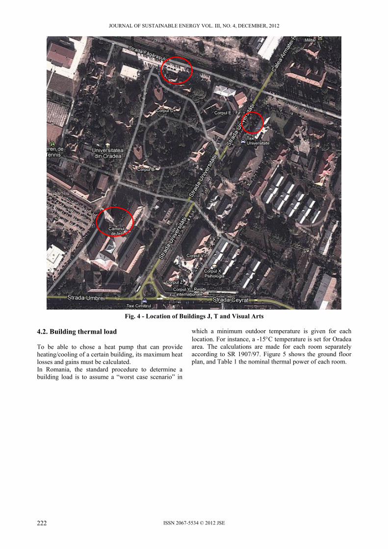
JOURNAL OF SUSTAINABLE ENERGY VOL. III, NO. 4, DECEMBER, 2012
ISSN 2067-5534 © 2012 JSE
Fig. 4 - Location of Buildings J, T and Visual Arts 4.2. Building thermal load To be able to chose a heat pump that can provide heating/cooling of a certain building, its maximum heat losses and gains must be calculated. In Romania, the standard procedure to determine a building load is to assume a “worst case scenario” in
which a minimum outdoor temperature is given for each location. For instance, a -15C temperature is set for Oradea area. The calculations are made for each room separately according to SR 1907/97. Figure 5 shows the ground floor plan, and Table 1 the nominal thermal power of each room.
222
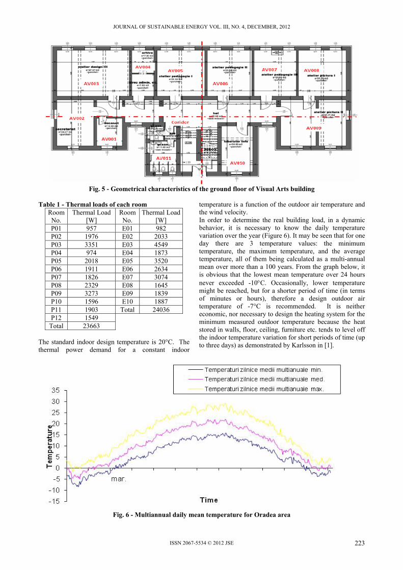
JOURNAL OF SUSTAINABLE ENERGY VOL. III, NO. 4, DECEMBER, 2012
ISSN 2067-5534 © 2012 JSE
Fig. 5 - Geometrical characteristics of the ground floor of Visual Arts building
Table 1 - Thermal loads of each room
Room No.
Thermal Load [W]
Room No.
Thermal Load[W]
P01 957 E01 982 P02 1976 E02 2033 P03 3351 E03 4549 P04 974 E04 1873 P05 2018 E05 3520 P06 1911 E06 2634 P07 1826 E07 3074 P08 2329 E08 1645 P09 3273 E09 1839 P10 1596 E10 1887 P11 1903 Total 24036 P12 1549
Total 23663 The standard indoor design temperature is 20°C. The thermal power demand for a constant indoor
temperature is a function of the outdoor air temperature and the wind velocity. In order to determine the real building load, in a dynamic behavior, it is necessary to know the daily temperature variation over the year (Figure 6). It may be seen that for one day there are 3 temperature values: the minimum temperature, the maximum temperature, and the average temperature, all of them being calculated as a multi-annual mean over more than a 100 years. From the graph below, it is obvious that the lowest mean temperature over 24 hours never exceeded -10C. Occasionally, lower temperature might be reached, but for a shorter period of time (in terms of minutes or hours), therefore a design outdoor air temperature of -7°C is recommended. It is neither economic, nor necessary to design the heating system for the minimum measured outdoor temperature because the heat stored in walls, floor, ceiling, furniture etc. tends to level off the indoor temperature variation for short periods of time (up to three days) as demonstrated by Karlsson in [1].
Fig. 6 - Multiannual daily mean temperature for Oradea area
223

JOURNAL OF SUSTAINABLE ENERGY VOL. III, NO. 4, DECEMBER, 2012
ISSN 2067-5534 © 2012 JSE
Based on these meteorological data, the monthly energy consumption of the building is presented in Table 2. Table 2 - Monthly thermal energy consumption of the building
Month Energy consumption [MWh] January 8090.16 February 6368.85 March 5387.70 April 3201.64 May 1566.39 June 344.26 July 0 August 0 September 1428.69 October 3494.26 November 5009.02 December 7246.72 42137.71
4.3. Heating system of the building The heating/cooling system of the building consists of radiant walls, PE pipes of 9.9 mm internal diameter and 1.1 mm wall thickness being placed on the walls at 8 cm spacing (Figure 7a), and covered with a special plaster. The flow is distributed to two sets of manifolds on each floor, each of them supplying about the same number of rooms. Based on the results presented in Table 1, the length of each circuit was calculated. Since it can’t exceed 60 m because of too high pressure losses, some of the rooms, having a large thermal load, will need several circuits. Figure 7b) shows the flow/return pipes of two circuits captured using a thermography camera. Each room has a temperature sensor which communicates by radio with a control valve on the supply pipe on the manifold. The corridors and restrooms on each floor are conditioned by 4 ceiling mounted fan coil units (one on each corridor, and one in each restroom).
a) b) Fig. 7 - Heating/cooling wall pipes
4.4. Heat Pump System The heat pump is a prototype (Figure 8) manufactured by OCHSNER Wärmepumpen GmbH (Austria). It is internally reversible and supplies heating and active cooling (no hot tap water). The heat pump also controls four 3-way valves to change the flow direction on the outdoor and indoor circuits. The nominal heating capacity is 37.3 kW and the nominal cooling capacity is 31.1 kW. According to the lab tests performed by the manufacturer in certain operating conditions, the heating capacity is 36.66 kW, the compressor’s electric power consumption is 6.5 kW, and the calculated COP is 5.64 (10% increase). Both the condenser and vaporizer are flat plate made of stainless steel 1.4401. The compressor is Scroll (full hermetic). The working fluid is R 407C.
Fig. 8 – Heat pump prototype
224

JOURNAL OF SUSTAINABLE ENERGY VOL. III, NO. 4, DECEMBER, 2012
ISSN 2067-5534 © 2012 JSE
4.5. Geothermal System Since a ground source heat pump system consists of three major components: the building heating/cooling system, the heat pump system, and the underground system, the last one is on focus now. First, we have to set the type of borehole heat exchanger, and consequently, to determine the length and number of boreholes, according to the building load, the heat pump heating capacity and COP. The borehole heat exchangers are single-U type with a shank spacing of 75 mm (spacers placed every 2.5 m), made of HDPE, the nominal diameter is 40 mm, with 2.4 mm wall thickness (Figure 9). The borehole heat exchangers are manufactured by UPONOR AB (Sweden).
a) b)
Fig. 9 – Borehole heat exchanger geometry
The selected borehole configuration (Figure 10) is due to the available space for drilling. The ground coupled system consists of 10 boreholes arranged in a rectangular grid (two lines of 5 boreholes each). The distance between adjacent boreholes is 10 meters. Each borehole has 130 m depth and 150 mm diameter. The grouting material is coarse sand from bottom to 10 m below surface, and bentonite for the upper 10 m to prevent the infiltration of warm water from a near-by thermal river to infiltrate in the boreholes, for allowing free cooling during low partial loads. The manifolds are located in a concrete cellar placed in the middle of the borehole field, and are connected to the heat pump by a supply and a return pipe placed 2 m below surface, same as the connections to the borehole heat exchangers.
The fluid in the outdoor loop is de-mineralized water with 10% mono-ethylene glycol to avoid freezing, as the system was started in heating mode in winter, with the indoor walls still wet. It is intended to replace the anti-freeze with plain water in the future, if measurements will show no freezing danger.
Fig. 10 – Borehole configuration: 2 x 5 rectangle
4.6. Hydraulic layout system The hydraulic layout for each type of operation (heating/active cooling/passive cooling) is shown in Figure 11. For passive cooling, a plate heat exchanger is needed, as the indoor circuit is filled with plain water, while the outdoor circuit is filled with a mixture of de-mineralized water with 10% mono-ethylene glycol. For heating and active cooling, a 1,000 l storage tank is placed between the heat pump and the indoor loop. A 7 kW electric resistance in the storage tank can be used for peak loads (and partial back-up). Since there are three major circuits, the hydraulic layout presents three circulation pumps, one for the geothermal circuit, one for the building circuit, and one between the heat pump and storage tank.
225

JOURNAL OF SUSTAINABLE ENERGY VOL. III, NO. 4, DECEMBER, 2012
ISSN 2067-5534 © 2012 JSE
Fig. 11 – The hydraulic layout out of Ground-Med Oradea demo-site
All the equipment mentioned in Figure 11 may be seen as built in Figure 12.
Fig. 12 – The technical room
4.7. Data acquisition and monitoring system The following parameters will be monitored by this system: external temperature, internal temperature, heat pump power consumption, external circulation pump power consumption, internal circulation pump power consumption, fan coil power consumption, internal circulation water flow, external circulation water flow, condenser inlet temperature, condenser outlet temperature, evaporator inlet temperature, evaporator outlet temperature.
Thermal energy on both indoor and outdoor loops are measured by Brunata energy meters, and 5 Carlo Gavazzi electric energy meters are used for the heat pump compressor, the outdoor circulation pump, the two indoor circulation pumps, the electric resistance in the storage tank, and the 4 fan coil units, respectively. All equipment is placed in a control box (see Figure 12). The data measured by these energy meters, as well as by an outdoor temperature sensor and a solar radiation sensor, are transmitted to a National Instruments controller, which also communicates with the heat pump controller (for data acquisition only).
Fig. 13 – The control box
226

JOURNAL OF SUSTAINABLE ENERGY VOL. III, NO. 4, DECEMBER, 2012
ISSN 2067-5534 © 2012 JSE
CONCLUSIONS GROUND-MED European project is an ambitious project that involves more than 20 partners from almost all European countries and aims to develop ground source heat pump systems that have higher seasonal performance factor than the ones used today. One of the 8 demonstration systems is located at University of Oradea. At an initial stage, a large building was chosen to be heated/cooled with this new system, but its poor insulation and old window frames extremely increased the heat losses of the building. Therefore, this building became inappropriate for installing a ground source heat pump system of medium capacity (20 -80 kW). We focused then to another building, a smaller one, having a heat loss of about 40 kW. For the base heating load, the highest specific heat extraction rate is in January (6.17 W/m) and the lowest is in September (1.06 W/m). Speaking of peak heating loads, the maximum value is 27.64W/m. For cooling, specific heat injection rate is 19.64 W/m. Therefore, depending to the outside temperature conditions, we may have two scenarios: either the weather conditions are mild and the system will run
base load, or – the worst case scenario – when the system has to run continually for several hours at maximum heat capacity and then, of course, specific heat extraction will be maximum. Consequently, the fluid output temperature will decrease substantially if peak loads occur. For instance, after 20 years of running base load, the minimum fluid temperature is at the end of January (7.52 C), but if the heat load occurs, the temperature will drop 6 C, reaching 1.41 C. The fluid temperature in every months of the heating season will decrease comparing with the temperatures for base heating load. If we take into consideration the cooling peak loads, the fluid temperature will be higher in summer months (July, August) comparing to the base load. After running the simulation and getting the fluid temperatures, we can conclude that the initial data are O.K. and the system will run with a SPF factor of at least 5.0. REFERENCES [1]. T. Karlsson, “Geothermal district heating. The Icelandic experience” UNU G.T.P., Orkustofnun, Reykjavik, Iceland, Report 4, 1984, 116 pp
227

JOURNAL OF SUSTENABLE ENERGY, VOL. III, NO. 4, DECEMBER, 2012
ISSN 2067-5534 © 2012 JSE
THERMAL STORAGE COUPLED TO A GROUND SOURCE HEAT PUMP IN A PUBLIC SERVICES BUILDING
CARVALHO A.*;**, QUINTINO A.*, FONG J.* and DE ALMEIDA A.*,
*Instituto de Sistemas e Robótica de Coimbra, University of Coimbra **Instituto Politécnico de Coimbra – Instituto superior de Engenharia
Abstract - Thermal storage may be a particularly attractive approach in service sector buildings, particularly for space conditioning, since it can help to reduce the electricity costs taking advantage of variable electricity rates while helping the grid to overcome the intermittent output of renewable energy. The aim of this paper is to describe globally the thermal storage system, which will be coupled to the ground source heat pump (GSHP), which was installed in a public building in Coimbra within the European Project from FP7 – Ground-Med. This project aims to demonstrate a high seasonal performance factor for ground source heat pumps (GSHP) that will be installed in pilot buildings in southern Europe. Keywords: Thermal Storage, Building, Electricity costs, GSHP, PCM, Phase-Change Materials. 1. INTRODUCTION
The increasing integration of intermittent nature renewable energy has led to the need to consider new ways of managing the grid since often this type of supply is out of line with periods of increased demand. It is therefore necessary to develop solutions that allow the flexible integration of production with energy consumption. Hence, thermal storage with phase change material can be one of the potential solutions for this problem [1, 2, 3].
In Portugal, during the night in rainy and windy winters, the production of electricity from renewable sources exceeds the needs of electricity consumption. For this reason, the study of an efficient thermal energy storage system for space heating is very important.
The pilot building in Coimbra, where the GSHP was installed, is a public service building with four floors where three floors are mainly offices. The GSHP was designed and installed to satisfy the thermal needs of the 3rd floor. This is the floor which presents higher thermal gains and losses due to its connection to the roof and due to the large glass area. This floor has 22 rooms (offices) and approximately a space conditioned area of 600 m2. The space conditioning system, which was installed before in this floor, was composed of two units (variable velocity compressors) with a heating capacity of 31,5 kW.
Fig. 1 - Pilot Building in Coimbra
The main electricity consumption is due to space
conditioning systems, office equipment and illumination. The period occupancy is from 8 AM to 7 PM as represented in the load profile of the building presented in Figure 2.
Fig. 2 - Electrical Load profile of the building – Mid-
winter It is possible to observe that the peak load of the
building occurs in the morning, when workers turn on all the electric equipment, including the space heating system. This peak load period is coincident with the national peak load demand period, where the electricity and the power have a higher price.
For the reasons presented before, the installation of a thermal storage will reduce the electricity bill of the building (moving consumption to lower cost off-peak periods) and reduce the peak power. For this purpose, it was decided that a latent heat thermal energy storage (LHTES) will be coupled to the GSHP.
Energy storage with phase change material (PCM) has a lot of advantages over sensible systems because of the lower mass and volume of the system, the energy is
228
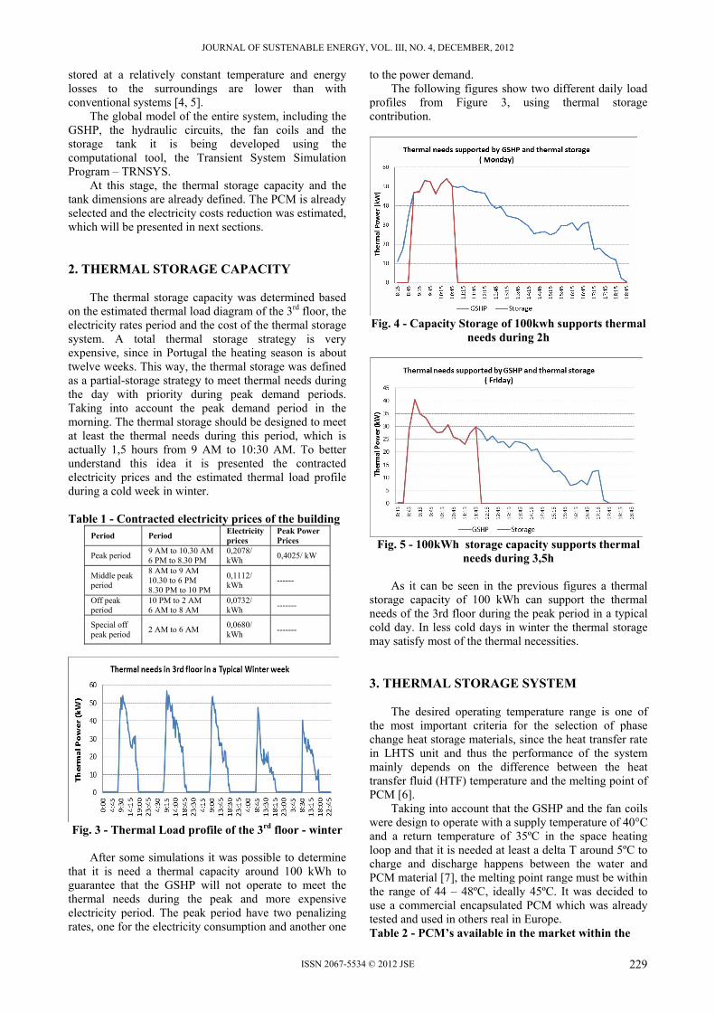
JOURNAL OF SUSTENABLE ENERGY, VOL. III, NO. 4, DECEMBER, 2012
ISSN 2067-5534 © 2012 JSE
stored at a relatively constant temperature and energy losses to the surroundings are lower than with conventional systems [4, 5].
The global model of the entire system, including the GSHP, the hydraulic circuits, the fan coils and the storage tank it is being developed using the computational tool, the Transient System Simulation Program – TRNSYS.
At this stage, the thermal storage capacity and the tank dimensions are already defined. The PCM is already selected and the electricity costs reduction was estimated, which will be presented in next sections. 2. THERMAL STORAGE CAPACITY
The thermal storage capacity was determined based
on the estimated thermal load diagram of the 3rd floor, the electricity rates period and the cost of the thermal storage system. A total thermal storage strategy is very expensive, since in Portugal the heating season is about twelve weeks. This way, the thermal storage was defined as a partial-storage strategy to meet thermal needs during the day with priority during peak demand periods. Taking into account the peak demand period in the morning. The thermal storage should be designed to meet at least the thermal needs during this period, which is actually 1,5 hours from 9 AM to 10:30 AM. To better understand this idea it is presented the contracted electricity prices and the estimated thermal load profile during a cold week in winter.
Table 1 - Contracted electricity prices of the building
Period Period Electricity prices
Peak Power Prices
Peak period 9 AM to 10.30 AM 6 PM to 8.30 PM
0,2078/ kWh
0,4025/ kW
Middle peak period
8 AM to 9 AM 10.30 to 6 PM 8.30 PM to 10 PM
0,1112/ kWh
------
Off peak period
10 PM to 2 AM 6 AM to 8 AM
0,0732/ kWh
-------
Special off peak period
2 AM to 6 AM 0,0680/ kWh
-------
Fig. 3 - Thermal Load profile of the 3rd floor - winter
After some simulations it was possible to determine
that it is need a thermal capacity around 100 kWh to guarantee that the GSHP will not operate to meet the thermal needs during the peak and more expensive electricity period. The peak period have two penalizing rates, one for the electricity consumption and another one
to the power demand. The following figures show two different daily load
profiles from Figure 3, using thermal storage contribution.
Fig. 4 - Capacity Storage of 100kwh supports thermal
needs during 2h
Fig. 5 - 100kWh storage capacity supports thermal
needs during 3,5h
As it can be seen in the previous figures a thermal storage capacity of 100 kWh can support the thermal needs of the 3rd floor during the peak period in a typical cold day. In less cold days in winter the thermal storage may satisfy most of the thermal necessities. 3. THERMAL STORAGE SYSTEM
The desired operating temperature range is one of the most important criteria for the selection of phase change heat storage materials, since the heat transfer rate in LHTS unit and thus the performance of the system mainly depends on the difference between the heat transfer fluid (HTF) temperature and the melting point of PCM [6].
Taking into account that the GSHP and the fan coils were design to operate with a supply temperature of 40°C and a return temperature of 35ºC in the space heating loop and that it is needed at least a delta T around 5ºC to charge and discharge happens between the water and PCM material [7], the melting point range must be within the range of 44 – 48ºC, ideally 45ºC. It was decided to use a commercial encapsulated PCM which was already tested and used in others real in Europe. Table 2 - PCM’s available in the market within the
229
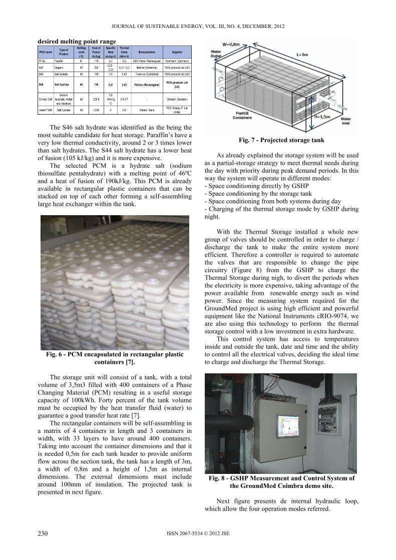
JOURNAL OF SUSTENABLE ENERGY, VOL. III, NO. 4, DECEMBER, 2012
ISSN 2067-5534 © 2012 JSE
desired melting point range
The S46 salt hydrate was identified as the being the most suitable candidate for heat storage. Paraffin’s have a very low thermal conductivity, around 2 or 3 times lower than salt hydrates. The S44 salt hydrate has a lower heat of fusion (105 kJ/kg) and it is more expensive.
The selected PCM is a hydrate salt (sodium thiosulfate pentahydrate) with a melting point of 46ºC and a heat of fusion of 190kJ/kg. This PCM is already available in rectangular plastic containers that can be stacked on top of each other forming a self-assembling large heat exchanger within the tank.
Fig. 6 - PCM encapsulated in rectangular plastic
containers [7].
The storage unit will consist of a tank, with a total volume of 3,5m3 filled with 400 containers of a Phase Changing Material (PCM) resulting in a useful storage capacity of 100kWh. Forty percent of the tank volume must be occupied by the heat transfer fluid (water) to guarantee a good transfer heat rate [7].
The rectangular containers will be self-assembling in a matrix of 4 containers in length and 3 containers in width, with 33 layers to have around 400 containers. Taking into account the container dimensions and that it is needed 0,5m for each tank header to provide uniform flow across the section tank, the tank has a length of 3m, a width of 0,8m and a height of 1,5m as internal dimensions. The external dimensions must include around 100mm of insulation. The projected tank is presented in next figure.
Fig. 7 - Projected storage tank
As already explained the storage system will be used
as a partial-storage strategy to meet thermal needs during the day with priority during peak demand periods. In this way the system will operate in different modes: - Space conditioning directly by GSHP - Space conditioning by the storage tank - Space conditioning from both systems during day - Charging of the thermal storage mode by GSHP during night.
With the Thermal Storage installed a whole new group of valves should be controlled in order to charge / discharge the tank to make the entire system more efficient. Therefore a controller is required to automate the valves that are responsible to change the pipe circuitry (Figure 8) from the GSHP to charge the Thermal Storage during nigh, to divert the periods when the electricity is more expensive, taking advantage of the power available from renewable energy such as wind power. Since the measuring system required for the GroundMed project is using high efficient and powerful equipment like the National Instruments cRIO-9074, we are also using this technology to perform the thermal storage control with a low investment in extra hardware.
This control system has access to temperatures inside and outside the tank, date and time and the ability to control all the electrical valves, deciding the ideal time to charge and discharge the Thermal Storage.
Fig. 8 - GSHP Measurement and Control System of
the GroundMed Coimbra demo site.
Next figure presents de internal hydraulic loop, which allow the four operation modes referred.
230
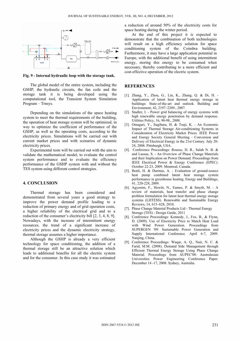
JOURNAL OF SUSTENABLE ENERGY, VOL. III, NO. 4, DECEMBER, 2012
ISSN 2067-5534 © 2012 JSE
Fig. 9 - Internal hydraulic loop with the storage tank.
The global model of the entire system, including the
GSHP, the hydraulic circuits, the fan coils and the storage tank it is being developed using the computational tool, the Transient System Simulation Program – Trnsys.
Depending on the simulations of the space heating
system to meet the thermal requirements of the building, the operation of heat storage system will be optimized, in way to optimize the coefficient of performance of the GSHP, as well as the operating costs, according to the electricity prices. Simulations will be carried out with current market prices and with scenarios of dynamic electricity prices.
Experimental tests will be carried out with the aim to validate the mathematical model, to evaluate the control system performance and to evaluate the efficiency performance of the GSHP system with and without the TES system using different control strategies.
4. CONCLUSION
Thermal storage has been considered and demonstrated from several years a good strategy to improve the power demand profile leading to a reduction of primary energy and of grid operation costs, a higher reliability of the electrical grid and to a reduction of the consumer’s electricity bill [2, 3, 4, 8, 9]. Nowadays, with the increase of intermittent energy resources, the trend of a significant increase of electricity prices and the dynamic electricity strategy, thermal storage assumes a higher importance.
Although the GSHP is already a very efficient technology for space conditioning, the addition of a thermal storage still be an attractive solution which leads to additional benefits for all the electric system and for the consumer. In this case study it was estimated
a reduction of around 50% of the electricity costs for space heating during the winter period.
At the end of this project it is expected to demonstrate that the combination of both technologies will result on a high efficiency solution for space conditioning system of the Coimbra building. Furthermore, it may have a large application potential in Europe, with the additional benefit of using intermittent energy, storing this energy to be consumed when necessary, thereby contributing to a more efficient and cost-effective operation of the electric system. REFERENCES [1]. Zhang, Y., Zhou, G., Lin, K., Zhang, Q. & Di, H. -
Application of latent heat thermal energy storage in buildings: State-of-the-art and outlook. Building and Environment, 42, 2197–2209., 2007.
[2]. Stadler, I. - Power grid balancing of energy systems with high renewable energy penetration by demand response. Utilities Policy, 16, 90-98., 2008.
[3]. Omagari, Y., Sugihara, H. & Tsuji, K. - An Economic Impact of Thermal Storage Air-conditioning Systems in Consideration of Electricity Market Prices. IEEE Power and Energy Society General Meeting - Conversion and Delivery of Electrical Energy in the 21st Century. July 20-24, 2008. Pittsburgh, USA.
[4]. Conference Proceedings: Rousse, D. R., Salah N. B. & and Lassue, S. - An Overview of Phase Change Materials and their Implication on Power Demand. Proceedings from IEEE Electrical Power & Energy Conference (EPEC). October 22-23, 2009. Montreal, Canada.
[5]. Benli, H. & Durmus, A. - Evaluation of ground-source heat pump combined latent heat storage system performance in greenhouse heating. Energy and Buildings, 41, 220-228, 2009.
[6]. Agyenim, F., Hewitt, N., Eames, P. & Smyth, M. - A review of materials, heat transfer and phase change problem formulation for latent heat thermal energy storage systems (LHTESS). Renewable and Sustainable Energy Reviews, 14, 615–628, 2010.
[7]. Phase Change Material Products Ltd - Thermal Energy Storage (TES) - Design Guide, 2011
[8]. Conference Proceedings: Kennedy, J., Fox, B., & Flynn, D. (2009). Use of Electricity Price to Match Heat Load with Wind Power Generation. Proceedings from SUPERGEN '09: Sustainable Power Generation and Supply International Conference. April 6-7, 2009. Nanjing, China.
[9]. Conference Proceedings: Waqar, A. Q., Nair, N. C. & Farid, M.M. (2008). Demand Side Management through Efficient Thermal Energy Storage Using Phase Change Material. Proceedings from AUPEC'08: Australasian Universities Power Engineering Conference Paper. December 14 -17, 2008. Sydney, Australia.
231

JOURNAL OF SUSTENABLE ENERGY, VOL. III, NO. 4, DECEMBER, 2012
ISSN 2067-5534 © 2012 JSE
EXPERIMENTAL STUDY ON POWER CHARACTERISTIC CURVES OF A PORTABLE PEM FUEL CELL STACK IN THE
SAME ENVIRONMENTAL CONDITIONS
CATĂRIG (RUS) T., RUS L.F. Technical University of Cluj-Napoca, Faculty of Building Services,
21 December 1989 no.128-130, Cluj-Napoca, [email protected]
Abstract – Due to the depletion of fossil fuels and greenhouse gases, fuel cells have received, in the last years, a special attention beeing a viable alternative for electricity necesities, and thermic in some cases. Fuel cells are considered one of the most promising devices due to its cleanliness, modularity, silence and high potential capability. In this paper is presented the principle of operation of a portable proton exchange membrane fuel cell stack and the power variation curve in same environmental conditions. Keywords: fuel cell stack, electrolyzer, storage canisters, USB data monitor. 1. INTRODUCTION
Fossil fuel reserves are finite and will be depleted in 50-100 years time. The continued use of fossil fuels generates greenhouse gases that are the cause of global warning and climate change [1].
The late of the 1990’s an international protocol, called Kyoto Protocol, aimed at fighting global warming. The goal of this protocol is to achieve the stabilisation of greenhouse gas concentrations in the atmosphere at a level that would prevent dangerous anthropogenic interference with climate system [2]. Because of the Kyoto Protocol and the development in science, fuel cells technology received an increasing attention from researchers and producers as beeing one of the future technology.
Fuel cells represent a radically different approach to energy conversion, one that could replace conventional power generation technologies.
The principle of operation of a fuel cell is almost as battery’s principle, ie electrochemical conversion. Fuel cells differ from conventional batteries in that they consume the reactant, which must be replenished continuously in a closed system. Another difference is that the electrodes within a battery change and become depleted during the charging and discharging cycle, whereas fuel cell electrodes are catalytic and relatively stable. By construction, the fuel cell structure remains invariable in time, meaning that as long as fuel and oxidant are provided the fuel cell will produce electricity (in some conditions).
2. THE OPERATING PRINCIPLE OF A PROTON EXCHANGE MEMBRANE (PEM) FUEL CELL
There are several types of fuel cells, but all are based on the same operational principle, namely electrochemical conversion. This is the direct transformation of chemical energy stored in various active materials into electrical energy [3]. Conversion is called direct because between the initial and final energy form is not interposed any other intermediate form.
Indirect energy conversion systems have more processing stages between which is found necessarily in the form of heat or mechanical. Direct conversion of energy eliminates mechanical or thermical energy link, achieving higher performance, which not depends on the limited efficiency of thermal machines, ie not depends on Carnot limits. The idea to obtain power by converting chemical energy directly occurred when the question of performing a reverse phenomenon in the electrolysis of water was made, that is to get electricity from the reaction between hydrogen and oxygen [4,5]. In figure 1 is presented a comparation between energy conversion of fuel cells, batteries and heat engines.
Fig. 1 - Schematic representation of energy
conversion of fuel cells, batteries and heat engines Basically, the energy released from oxidation of
conventional fuels, generally used as heat can be converted directly into electricity with great efficiency. As in nearly all the oxidation reactions involved in electron transfer between fuel and oxidizer, it is obvious that the chemical energy of oxidation can be converted directly into electricity.
Achieving direct conversion of chemical energy into electrical energy can not run without an element that contains an anode, a cathode and an electrolyte that can be fed directly with fuel and air, as is shown in figure 2.
Fuel rich in hydrogen (or pure hydrogen) is
232
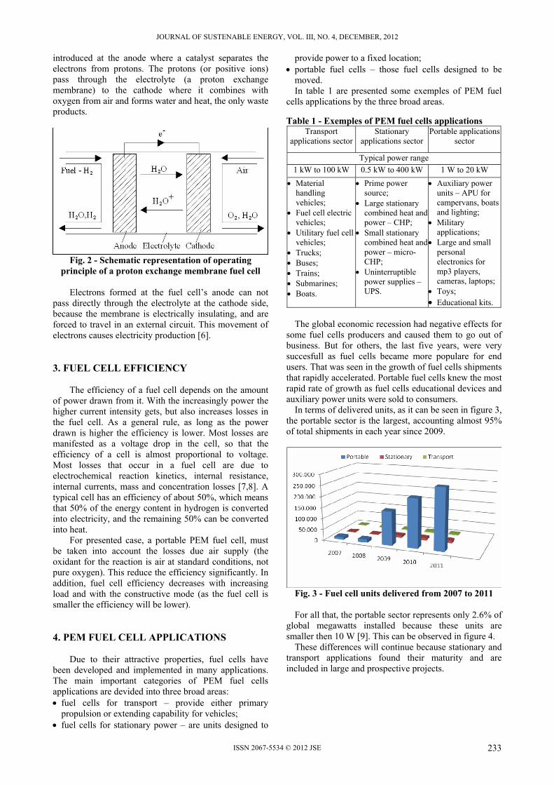
JOURNAL OF SUSTENABLE ENERGY, VOL. III, NO. 4, DECEMBER, 2012
ISSN 2067-5534 © 2012 JSE
introduced at the anode where a catalyst separates the electrons from protons. The protons (or positive ions) pass through the electrolyte (a proton exchange membrane) to the cathode where it combines with oxygen from air and forms water and heat, the only waste products.
Fig. 2 - Schematic representation of operating
principle of a proton exchange membrane fuel cell Electrons formed at the fuel cell’s anode can not
pass directly through the electrolyte at the cathode side, because the membrane is electrically insulating, and are forced to travel in an external circuit. This movement of electrons causes electricity production [6].
3. FUEL CELL EFFICIENCY The efficiency of a fuel cell depends on the amount
of power drawn from it. With the increasingly power the higher current intensity gets, but also increases losses in the fuel cell. As a general rule, as long as the power drawn is higher the efficiency is lower. Most losses are manifested as a voltage drop in the cell, so that the efficiency of a cell is almost proportional to voltage. Most losses that occur in a fuel cell are due to electrochemical reaction kinetics, internal resistance, internal currents, mass and concentration losses [7,8]. A typical cell has an efficiency of about 50%, which means that 50% of the energy content in hydrogen is converted into electricity, and the remaining 50% can be converted into heat.
For presented case, a portable PEM fuel cell, must be taken into account the losses due air supply (the oxidant for the reaction is air at standard conditions, not pure oxygen). This reduce the efficiency significantly. In addition, fuel cell efficiency decreases with increasing load and with the constructive mode (as the fuel cell is smaller the efficiency will be lower).
4. PEM FUEL CELL APPLICATIONS Due to their attractive properties, fuel cells have
been developed and implemented in many applications. The main important categories of PEM fuel cells applications are devided into three broad areas: fuel cells for transport – provide either primary
propulsion or extending capability for vehicles; fuel cells for stationary power – are units designed to
provide power to a fixed location; portable fuel cells – those fuel cells designed to be
moved. In table 1 are presented some exemples of PEM fuel
cells applications by the three broad areas. 5 W to 20 kW 0.5 kW to 400 kW 1 kW to 100 kW
Table 1 - Exemples of PEM fuel cells applications Transport
applications sectorStationary
applications sector Portable applications
sector
Typical power range
1 kW to 100 kW 0.5 kW to 400 kW 1 W to 20 kW
Material handling vehicles;
Fuel cell electric vehicles;
Utilitary fuel cell vehicles;
Trucks; Buses; Trains; Submarines; Boats.
Prime power source;
Large stationary combined heat and power – CHP;
Small stationary combined heat and power – micro-CHP;
Uninterruptible power supplies – UPS.
Auxiliary power units – APU for campervans, boats and lighting;
Military applications;
Large and small personal electronics for mp3 players, cameras, laptops;
Toys; Educational kits.
The global economic recession had negative effects for
some fuel cells producers and caused them to go out of business. But for others, the last five years, were very succesfull as fuel cells became more populare for end users. That was seen in the growth of fuel cells shipments that rapidly accelerated. Portable fuel cells knew the most rapid rate of growth as fuel cells educational devices and auxiliary power units were sold to consumers.
In terms of delivered units, as it can be seen in figure 3, the portable sector is the largest, accounting almost 95% of total shipments in each year since 2009.
Fig. 3 - Fuel cell units delivered from 2007 to 2011 For all that, the portable sector represents only 2.6% of
global megawatts installed because these units are smaller then 10 W [9]. This can be observed in figure 4.
These differences will continue because stationary and transport applications found their maturity and are included in large and prospective projects.
233

JOURNAL OF SUSTENABLE ENERGY, VOL. III, NO. 4, DECEMBER, 2012
ISSN 2067-5534 © 2012 JSE
Fig. 4 - Megawatts installed from 2007 to 2011
5. EXPERIMENTAL SET-UP
The experimental study was held in the Research Laboratory of the Faculty of Building Services of the Technical University from Cluj-Napoca that has an educational kit called “Clean Energy Trainer”. The goal of this educational kit is to familiarize the students with the interrelationship of renewable energy sources and hydrogen, but beyond this goal, the educational kit can be used in some experimental research studies. The educational kit has in his componence: two solar modules, a wind generator, two electrolyzers, four storage canisters, a fuel cell stack, a USB data monitor, a software, a consumer (a house with two lamps), an anemometer, a luxmeter, a fan, a lamp, bottle with distilled water, stop watch, hoses and cables. This components can be used in different ways, but for the experimental study were included only those that can be used with the fuel cell stack.
5.1. Electrolyzers and storage canisters
In order to be able to operate the fuel cell stack, hydrogen must be available. This can be produced with the electrolyzers (see fig. 5) by decomposing distilled water into hydrogen and oxygen. Distilled water is used to avoid poisoning the proton exchange membrane of the fuel cells with possible impurities.
Fig. 5 - An electrolyzer used to produce hydrogen
The electrolyzers can be powered from the solar
modules, or USB data monitor or the wind generator. For
the presented case the USB data monitor was used. The electrolyzers have each an hydrogen production
of 5 cm3/min and an oxygen production of 2.5 cm3/min, ie two parts hydrogen and one part oxygen. The constructive dimensions of an electrolyzer are LxWxH (length, width, height) 57x40x50 mm and weights 54 g.
The hydrogen and oxygen produced by the electrolyzers are stored in storage canisters (see fig. 6).
Fig. 6 - Storage canisters for hydrogen and oxygen
The storage canisters have a capacity of 30 cm3 and
are provided with hoses that lead the fluids to the fuel cell stack. The hoses have clips that gives us the posibility to open or close the fluid circuit.
5.2. USB data monitor and Clean Energy Trainer software
The USB data monitor (see fig. 7) can be used as a DC
voltage sources (as in the case of electrolyzers), as a source, as a measuring device and as a drain simulator. With this device and proper software investigations for analysing components and investigating systems can be made.
Fig. 7 - The USB data monitor
The USB data monitor has a maximum power of 10 W,
the voltage for the eletrolysis mode is between 0÷4 V and for the fuel cell mode is between 0÷10 V. The current for the eletrolysis mode is between 0÷3 A and for the fuel cell mode is between 0÷4 A. The dimensions of the USB data monitor are 160x1000x40 mm and weights 1400 g.
234

JOURNAL OF SUSTENABLE ENERGY, VOL. III, NO. 4, DECEMBER, 2012
ISSN 2067-5534 © 2012 JSE
With the Clean Energy Trainer software, that has an interface like in figure 8, various characteristic curves can be recorded. The software can operate in manual and in automatic mode.
Fig. 8 - The software’s interface
The software is divided into the respective thematic
blocks through various tabs: solar module, wind generator, electrolyzer, fuel cell, simulate generator profile, simulate load profile. 5.3. Fuel cell stack
With the fuel cell stack, hydrogen is converted into electrical energy and can be used by a consumer. The fuel cell stack, presented in figure 9, of the Clean Energy Trainer educational kit is compound with five fuel cells that can be taken apart. In doing so, it is possible to represent different levels of output.
Fig. 9 - The fuel cell stack
The fuel cell stack has a maximum power of 1 W.
The power of each fuel cell is 200 mW. The voltage generated by each cell can be between 0.4 and 0.96 V. The constructive dimensions of the fuel cell stack are LxWxH 175x70x60 mm and weights 430 g. In figure 10 are presented the five individual fuel cells.
Fig. 10 - The five fuel cells that compound the stack
5.4. Achievement of the experimental installation
In order determine the characteristic curves of the fuel cell stack the experimental installation must be set-up. At first it is necessary to connect the electrolyzers to the storage canisters to the USB data monitor and to a PC in order to generate hydrogen. Here, the USB data monitor is used as a DC voltage source for the electrolyzers. After hydrogen is produced, the fuel cell stack is connected to the canisters were hydrogen was stored in. The hydrogen outlet of the fuel cell stack is opened for one second and then closed to flush the fuel cell stack. Since impurities can collect on the hydrogen side during the operation of the fuel cell stack, it must be flushed regularly in order to maintain a sufficiently high concentration of hydrogen in the fuel cell. After the fuel cell stack is flushed, hydrogen must be generated again to complete the storage canisters with the quantity of hydrogen used for flushing the stack. Then the USB data monitor is disconnected from the electrolyzers and connected to the fuel cell stack, as is shown in figure 11.
Fig. 11 - The experimental set-up
235

JOURNAL OF SUSTENABLE ENERGY, VOL. III, NO. 4, DECEMBER, 2012
ISSN 2067-5534 © 2012 JSE
6. RESULTS AND DISCUSSION
Although a single storage canister has a capacity of 30 cm3 of fluid, the measurements on voltage, current and power of the fuel cell stack were performed with 10 cm3 respectively 15 cm3 of fuel.
The measurements on the fuel cell stack, with different quantity of hydrogen, were performed in same conditions, ie automatic mode of the Clean Energy Trainer software, at atmospheric pressure and an ambiental temperature of 21.1°C.
The experimental plant was put into operation, the outlet of hydrogen and air of the fuel cell stack was opened until the imposed quantity of fuel was consumed. The results obtained were recorded and centralised by the software through graphs that are presented in figure 12 and 13.
Fig. 12 - The current-voltage characteristic curve and the power characteristic curve obtained with 10 cm3
of hydrogen
Fig. 13 - The current-voltage characteristic curve and the power characteristic curve obtained with 15 cm3
of hydrogen
In the following will be presented voltage drops that
occur in a fuel cell with the exemplification on the current-voltage characteristic curve of the first graph.
The theoretically possible voltage of a hydrogen fuel cell in standard conditions is 1.23V. In practice and in this case losses occur through kinetic inhibition of the reaction, internal resistance and insufficient diffusion. Therefore the delivered voltage of an individual cell, like it was presented earlier, is actually 0.4÷0.9 Volts.
The difference between the theoretical voltage and delivered voltage is called overvoltage and is caused by the speed of the conversion of hydrogen and oxygen. On graphs, the overvoltage occurs and can be observed between the values of 0÷100 mA of the current. Between the values 100 mA and 300 mA appears the internal resistance which is caused by the resistance against the current flow in the electrolyte. Here the voltage decreases linearly with the increase of the current.
In the first graph near the value of 300 mA and 2 V the maximum power is reached. After that, the diffusion overvoltage occurs due to the faster consumption of the gases by the electrochemical reaction at the catalyst. A typical sign for this diffusion overvoltage is a sudden downward bend of the current-voltage characteristic curve. In this graph, after the diffusion overvoltage occurs, it can be observed a straight horizontal line between the value of 400 mA and 650 mA. This line is explained by the fact that, even the 10 cm3 of hydrogen were consumed, an insignificant quantity of hydrogen, for the process, is still in the cells and the software is recording continuously dates, until the whole quantity of hydrogen will be used.
In the second graph the diffusion overvoltage can not be observed as well as in the first graph, but it occur. Because the amount of hydrogen in this case is higher, the diffusion overvoltage is more extended from the first graph. The straight horizontal line it can be seen as well as in the first case with the same explanations.
In the table 2 are presented the maximum and the average power obtained in each experimental study.
Table 2 - The values extracted from the power characteristic curves of each study
Study 1with 10 cm3 of hydrogen
Study 2 with 15 cm3 of hydrogen
Pmax
0.6 W 0.56 W
Paverage
0.23 W 0.32 W
From table 2 can be observed that maximum power in
study 1 is higher than in study 2, but the average power is smaller than in the second case. Even if at first it was expected that the maximum power and the average power from the first study, the one performed with 10 cm3 of hydrogen, to be smaller than in the second study, in reality the maximum power obtained in the first case is higher than the second one due to the slowly voltage decrease. This slightly decrease can be put into the account of internal losses that can vary greatly especialy at a small installation, like the one that measurements were made on. It is also possible that the incurred losses
236

JOURNAL OF SUSTENABLE ENERGY, VOL. III, NO. 4, DECEMBER, 2012
ISSN 2067-5534 © 2012 JSE
during the process of electricity production to be a result of small quantity of fuel used.
If the two study cases are compared and it goes from the fact that “as long as the power drawn is higher the efficiency is lower” it can be assumed that using a smaller amount of hydrogen for electricity production is more efficient than using a larger amount of hydrogen, and that is correct.
7. CONCLUSION
Considering that PEM fuel cell stack can have a maximum power of 1 W, one can appreciate that the values resulted from the experiment are relatively acceptable. The losses that occur in a portable PEM fuel cell stack are very important and can reduce significantly the efficiency of fuel cell stack.
Although measurements made in the Research Laboratory of the Faculty of Building Services on the educational kit, did not led to noticeable conclusions on the possible improvements that can be done for reducing voltage losses and increasing power extracted from the fuel cell stack, because the experimental stand has a small operating capacity, some conclusions were made: at a small amount of hydrogen the diffusion
overvoltage is higher; at a larger quantity of hydrogen the voltage losses are
lower; at a larger quantity of hydrogen the power
characteristic curve does not present a downward bend, has a linear ascension/descension;
by using a large amount of hydrogen the current and the voltage will be higher, and so the power characteristic curve will be improved; To reach maximum power offered by educational kit,
might try to modify ambient parameters, namely to rise the ambient temperature, and to be observe what
influence has on the power. But this study will be the subject to a following experiment.
ACKNOWLEDGEMENTS This paper was supported by the project "Improvement of the doctoral studies quality in engineering science for development of the knowledge based society-QDOC” contract no. POSDRU/107/1.5/S/78534, project co-funded by the European Social Fund through the Sectorial Operational Program Human Resources 2007-2013. REFERENCES [1]. Ferng, Y.M., a.o. – Analytical and experimental
investigations of a proton exchange membrane fuel cells, International Journal of Hydrogen Energy, Elsevier, 2004, pp 381-391
[2]. www.en.wikipedia.org/wiki/Kyoto_Protocol [3]. Stefanescu, I., Pile de combustibil – între teorie şi practică,
Conphys eds., Râmnicu Vâlcea, Romania, 2010 [4]. Gevorkian, P., Alternative energy systems in building
design, Mc Graw Hill, United States of America, 2010 [5]. DaRosa, A.V., Fundamentals of renewable energy
processes, Elsevier Academic Press, California, United States of America, (2006)
[6]. Badea, G., Catarig, T., - Obtinerea curbei de polarizare intr-o pila de combustibil cu membrana schimbatoare de protoni, Conferinta Stiinta Moderna si Energia, Ed. Risoprint, Cluj-Napoca, Romania, 2012
[7]. Catarig, T. – Utilizarea pilelor de combustibil pentru producerea energiei electrice si termice. Stadiu actual, analiza critica si concluzii., Raport de cercetare stiintifica, Cluj-Napoca, Romania, 2012
[8]. Barbir, F., PEM Fuel Cells: Theory and Practice, Elsevier Academic Press, New York, United States of America, 2005
[9]. www.fuelcelltoday.com, Fuel Cell Today – The Industry Review, 2011
237

JOURNAL OF SUSTAINABLE ENERGY, VOL. III, NO. 4, DECEMBER, 2012
ISSN 2067-5534 © 2012 JSE
THE LOAD FREQUENCY CONTROL SIMULATION OF A THERMAL GENERATOR INTERCONECTED
ON AN INFINITE BUS BARS
MIRCEA I., IOVAN G., POPESCU D. University of Craiova, Faculty of Electrical Engineering
Abstract: In this paper is presented the simulation of the behavior in load frequency control for a power thermal generator interconnected with an infinite bus bars, generated by the frequency variations, caused by imbalances of production consumption balance. By using the MATLAB_SIMULINK in order to follow the time evolution of the angular speed / frequency and how to mobilize the primary control reserve a thermal generator of 330 MW by simulating the frequency variation in the infinite bus bars. Key words: load frequency, infinite bus bars, power thermal generator. 1. INTRODUCTION:
It follows the static stability in combined turbine and generator to small frequency oscillations operating conditions generated by the electrical power disturbances. Generally, these oscillations arise from the transmission and distribution tie lines to generating units. These oscillations are classified into the following types [6]: - Inter-area oscillations with the typical oscillation between 0.1 - 0.7 Hz, the most interest in terms of primary control LFC . - Local plant oscillations with the typical oscillation between 0.8- 2Hz. - Intra-plant oscillations with the typical oscillation between 1.5 - 3 Hz. of interest in terms of their local stabilization.
The article aims to show how to approach the mathematical modeling and simulation the primary control LFC for thermal generators.
2. The mathematical modeling of the synchronous generators connected to the network.
Starting from the oscillation equation of synchronous machine [6] linearized to small perturbations connected to a infinite bus bars we consider the mechanical power Pm = ct.:
Pm – Pe = Pa = 0 (acceleration power) (1)
0TDdt
dH2 12
p.u. (2)
dtfdt p.u. (3)
Where:
Pm = the mechanical power Pe = the electric power Pa = the acceleration power D = the damping constant [5] T12 = the synchronization constant H = the synchronization constant time r.u.
The first term represents the inertia of the angular speed (frequency in r.u), the second term represents the damping power and the last term represents and synchronization power.
The frequency of free oscillation to small disturbances in r.u. is:
M
Tf 12
0 [p.u.]. (4)
The moment of inertia is:
SS
C H2
f2
E2M
[ sHz
..u.p ] (5)
In the literature [5] the inertia constant H is obtained by
kinetic energy divided to the nominal apparent power Sn:
n
C
S
EH [p.u. s] (6)
For 1cos in the transport network, we can write
without significant errors, the S [MVA] = P [MW] and we obtain the time constant of inertia:
H2M (7) M = 2H is the turbine / generator axis constant of inertia [sec]
From (2) to determine that Mmin and Hmin, we use the following relationship [7]:
238

JOURNAL OF SUSTAINABLE ENERGY, VOL. III, NO. 4, DECEMBER, 2012
ISSN 2067-5534 © 2012 JSE
PfDdt
df
f
H2
0
(8)
and neglecting the damping factor of the load D [ur / Hz] we obtain:
H2
fP
dt
df 0 [Hz/s]RELdt
df
(9)
REL
0min
dt
df2
fPH
(10)
Were : f0 = nominal frequency in the system (pre-disturbance)
LT
L
PP
PP
(11)
the amplitude of perturbation in the system u.r.
LP = the local perturbation [MW]
PT = the total power produced (pre-disturbance).
RELdt
df
= 0,1[Hz/s]
the value that is set the accelerometer relay. The accelerometers relay is set to 0.1 [Hz / sec]. Many relays are set to 0.2 [Hz / sec] The accelerometers relays used in SEN are numerical MICOM P941 and P943 type from AREVA. Relay measures the changes in frequency in a time of = 100
[msec] and calculate dt
df every 25 [ms]. If the
calculated value exceeds a prescribed value more than 50 samples relay acts [7].
Typical values of inertia constant H [7] are presented in the table below (Table 1).
Table 1 - Typical values of inertia constant H for generators No. crt.
The generators type H [sec]
Hydro generators Low speed (< 200rot/min) 2 – 3
1
High speed (> 200rot/min) 2 – 4 Termal generators
With condensing (1500rot/min) 6 – 9 With condensing (3000rot/min) 4 – 7
2
Without condensing (3000rot/min) 3 - 4 3 synchronous motors for heavy
shareholders 2
The T12 constant synchronization ( the sync torque) is the "rigid" connection with the infinite bus bars:
)0(
)0(
T
q12
Pcos
X
EUT
(12)
Were : = the power angle.
)0( = the power angle were the linearization is made Eq = the electromotive voltage behind synchronous reactance. U = the infinite bus bars voltage . XT = Xd + Xtr. bloc + Xretea representing the total reactance across the generator terminals. The generator active power pre-disturbance.
)0(max
)0(
T
q)0( sinPsinX
EUP
(13)
To study the frequency stability and the behavior of generators in the primary control is used the following simplifying assumptions: - The loads are represented by admittance.. - Synchronous machines are represented as ideal voltage
sources and equal to 'qE behind their internal synchronous
reactance reactance Xd and the internal reactance of the
machine is equal with transient reactance 'dX [5].
- The generator terminals voltage is constant. Depending on the total reactance of the machine terminals will operate in the unperturbed system at different load angles, thus obtaining different values for synchronizing constant T12. As seen from (4) timing and constant values of the moment of inertia will influence the dynamic behavior of the angular speed / frequency. For Heat-synchronous PN = 330 MW nominal power operating at 80% of rated power at power angle = 250 (Pmax = 638MW). The synchronization constant values u.r. for different loads are represented in table (Tab.2.)
Table 2 - The synchronization constants depending on power angle
Angle )0( 50 100 150 200 250
T12 u.r. 1.93 1,9 1,86 1,8 1,75
Pe u.r. 0,16 0,33 0,5 0,66 0,8
If total the reactance on generator terminals decreases (shorter evacuation tie line) the evacuation power Pmax will increases and the evacuation of power will be made at a lower power angle by a greater synchronizing factor T12. For example, for a total reactance lower with 20% (Pmax = 789MW) the synchronizing constants are (see Table 3.)
Table 3 - The synchronization constants depending on
power angle . Angle
)0(
50 100 150 200 250
T12 u.r. 2,38 2,35 2,3 2,24 2,16
Pe u.r. 0,2 0,4 0,6 0,8 1
239
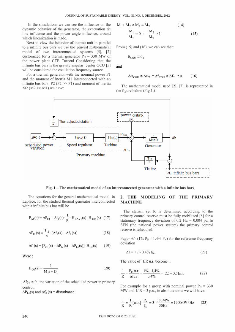
JOURNAL OF SUSTAINABLE ENERGY, VOL. III, NO. 4, DECEMBER, 2012
ISSN 2067-5534 © 2012 JSE
In the simulations we can see the influence on the dynamic behavior of the generator, the evacuation tie line influence and the power angle influence, around which linearization is made. Next to view the behavior of thermo unit in parallel to a infinite bus bars we use the general mathematical model of two interconnected systems [5], [2] customized for a thermal generator PN = 330 MW of the power plant CTE Turceni. Considering that the infinite bus bars is the gravity angular center GCU [5] will be considered the oscillation frequency source. For a thermal generator with the nominal power P1 and the moment of inertia M1 interconnected with an infinite bus bars P2 (P2 >> P1) and moment of inertia M2 (M2 >> M1) we have:
T221 MMMM (14)
0M
M
T
1 ; 1M
M
T
2 (15)
From (15) and (16), we can see that:
2CGU
and
2CGU = 2CGU ff r.u. (16)
The mathematical model used [2], [7], is represented in
the figure below (Fig.1.)
Fig. 1 – The mathematical model of an interconnected generator with a infinite bus bars
The equations for the general mathematical model, in Laplace, for the studied thermal generator interconnected with a infinite bus bar will be
)s(H)s(HR
1)s(fP)s(P 1TB1RAV11C1m (17)
)]s(f)s(f[s
T)s(P 21
1212 (18)
)s(H)]s(P)s(P)s(P[)s(f 1G1L121m1 (19)
Were :
111G DsM
1)s(H
(20)
0P 1C ; the variation of the scheduled power in primary
control. ∆PL1(s) and ∆f2 (s) = disturbance.
2. THE MODELING OF THE PRIMARY MACHINE The statism set R is determined according to the primary control reserve must be fully mobilized [8] for a stationary frequency deviation of 0.2 Hz = 0.004 pu. In SEN (the national power system) the primary control reserve is scheduled: PREG= +/- (1% PN - 1.4% PN) for the reference frequency deviation
Δf = + / - 0.4% fN. (21) The value of 1/R u.r. become :
.r.u]5,35,2[%4,0
%4,1%1
.r.fu
.r.uP
R
1 Re
(22)
For example for a group with nominal power PN = 330 MW and 1/ R = 3 p.u., in absolute units we will have:
Hz/MW8,19Hz50
MW3303
f
P.]r..u[
R
1
R
1
N
N (23)
240

JOURNAL OF SUSTAINABLE ENERGY, VOL. III, NO. 4, DECEMBER, 2012
ISSN 2067-5534 © 2012 JSE
The active power mobilized in primary control for the reference incident Δf = + / - 0.2 Hz
MW96,3Hz/MW8,19Hz2,0fR
1P gRe (24)
The primary control band will be :
BReg = 2PReg = 7,92 MW 2,5%PN (25) 3. THE STATIC SPEED REGULATOR PI TYPE
The practicality model of the static speed regulator is represented in diagrams below (Fig.2.)
a
b
c
Fig. 2 – The static loop regulation model a) schematic diagram; b) block diagram; c) the
equivalent block diagram
Were: SI = intermediate actuator PC = the schedule active power oscillations . RAV = automatic speed regulator typed (I,PI,PID) R = the permanent statism.
RKK 1 the proportionality factor regulator [MW/Hz]
The proportionality constant K [MW / Hz], given the general structure of the RAV should be proportional to 1/R :
R
KK 1 [MW/Hz] (26)
The mathematical model used is: (Fig. 3).
Fig. 3 – The mathematical model of the PI static regulator RAV
We will use the technical data for static PI RAV
model (The CTE Turceni power plant model) PI type with it’s proper constants : KP =1; TI = 1,5 sec, TSI = 1,25 sec [K1 = 5, R = 0,33 u.r.
The RAV regulator transfer function will be:
33,33s60s
33,33s50
R
1H
2T)EERAV(
(27)
The mathematical model used in stability studies for steam turbines is a simplified model with transfer function [1] ,[2]:
)sT1)(sT1(
sTF1)s(H
CHRH
RHHPTB
(28)
The typical constants for steam turbine with overheating cycle is : [2 ]:
FHP = 0,3 ; TRH = (5 -7) s ; TCH = 0,3 s. For the constant time TRH = 5 sec specific for the steam turbines with overheating cycle the transfer function (30) will becomes:
1s3,5s5,1
1s5,1)s(H
2TB
(29)
The disturbances in the infinite power system are done
by simulating different frequency deviations of amplitude and time evolution (step signal or ramp signals at different rates of change of frequency in time). The qualification tests in primary control [8] are simulated used a frequency step deviation in upward or downward. The frequency deviation level in this case is maximum because in reality the frequency deviation after imbalance between production and consumption has a finite speed variation that depending on the inertia moment of the system generators and the consumption damping factor D [MW/Hz].
The cconstants necessary for the simulation of mathematical model are summarized in the table below (Table 4.)
241
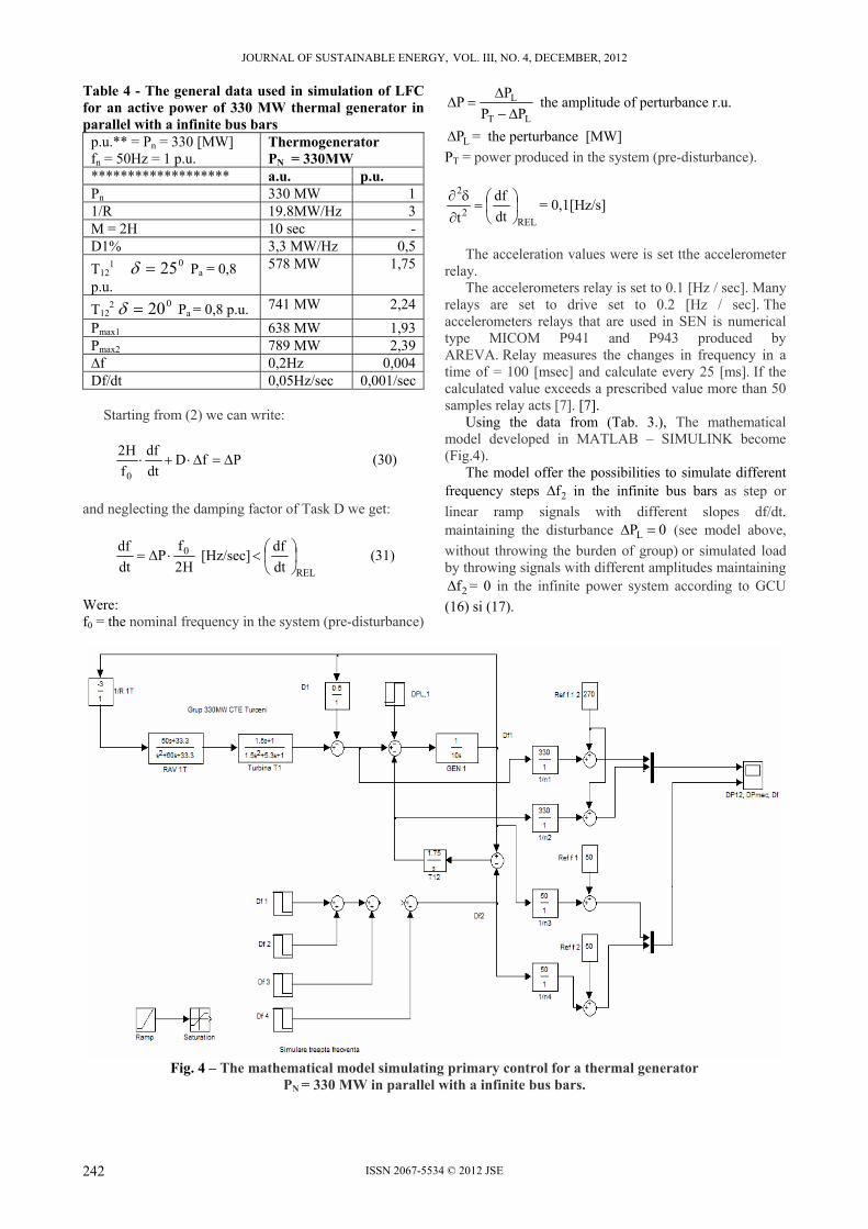
JOURNAL OF SUSTAINABLE ENERGY, VOL. III, NO. 4, DECEMBER, 2012
ISSN 2067-5534 © 2012 JSE
Table 4 - The general data used in simulation of LFC for an active power of 330 MW thermal generator in parallel with a infinite bus bars
p.u.** = Pn = 330 [MW] fn = 50Hz = 1 p.u.
Thermogenerator PN = 330MW
******************* a.u. p.u. Pn 330 MW 1 1/R 19.8MW/Hz 3 M = 2H 10 sec - D1% 3,3 MW/Hz 0,5
T121 025 Pa = 0,8
p.u.
578 MW 1,75
T122 020 Pa = 0,8 p.u. 741 MW 2,24
Pmax1 638 MW 1,93 Pmax2 789 MW 2,39 ∆f 0,2Hz 0,004 Df/dt 0,05Hz/sec 0,001/sec
Starting from (2) we can write:
PfDdt
df
f
H2
0
(30)
and neglecting the damping factor of Task D we get:
H2
fP
dt
df 0 [Hz/sec]RELdt
df
(31)
Were: f0 = the nominal frequency in the system (pre-disturbance)
LT
L
PP
PP
the amplitude of perturbance r.u.
LP = the perturbance [MW]
PT = power produced in the system (pre-disturbance).
REL2
2
dt
df
t
= 0,1[Hz/s]
The acceleration values were is set tthe accelerometer
relay. The accelerometers relay is set to 0.1 [Hz / sec]. Many
relays are set to drive set to 0.2 [Hz / sec]. The accelerometers relays that are used in SEN is numerical type MICOM P941 and P943 produced by AREVA. Relay measures the changes in frequency in a time of = 100 [msec] and calculate every 25 [ms]. If the calculated value exceeds a prescribed value more than 50 samples relay acts [7]. [7].
Using the data from (Tab. 3.), The mathematical model developed in MATLAB – SIMULINK become (Fig.4).
The model offer the possibilities to simulate different frequency steps 2f in the infinite bus bars as step or
linear ramp signals with different slopes df/dt. maintaining the disturbance 0PL (see model above,
without throwing the burden of group) or simulated load by throwing signals with different amplitudes maintaining
2f = 0 in the infinite power system according to GCU
(16) si (17).
Fig. 4 – The mathematical model simulating primary control for a thermal generator PN = 330 MW in parallel with a infinite bus bars.
242

JOURNAL OF SUSTAINABLE ENERGY, VOL. III, NO. 4, DECEMBER, 2012
ISSN 2067-5534 © 2012 JSE
Below are represented the diagrams obtained for different disturbances using the model from Figure 4. for time period t = 60 sec.
Fig. 5 – The thermal generator response to a frequency variation step ΔfT or ramp. ΔfR ∆fT = 0,2Hz (0,004p.u..) step ; ∆fR = 0,2Hz
V=0,05Hz/sec ( V= 0,001p.u./sec) ramp; For the generator: ∆fGT =The frequency variation to
the step signal . ∆fGR = The frequency variation to the ramp signal. ∆PET, ∆PMT = the variation of the electrical and
mechanical power for the step signal frequency . ∆PER, ∆PMR = the variation of the electrical and
mechanical power for the ramp signal frequency
Fig. 6 – The thermal generator response to the
frequency step variation. ∆fT = 0,2Hz (0,004u.r.) pentru T12
1 >T122
Fig. 7 – The primary control reserve mobilization to a
frequency variation in four 50MHz level steps. a) the electric variation and the mechanical power
variation b) frequency variation
243

JOURNAL OF SUSTAINABLE ENERGY, VOL. III, NO. 4, DECEMBER, 2012
ISSN 2067-5534 © 2012 JSE
Fig. 8 – The qualification test in primary control
group of 330 MW thermal CTE Turceni (∆f = 4 x 0,05Hz., in power regulation, the turbina
lead)
The mathematical model for determining the equivalent transfer function is the generally insular one completed with the interconnection tie line, resulting the general model for an interconnected systems in radial network, as shown below ( Fig. 9. a); b) ;Fig. 10. a); b); c).
Fig .9 – The general insular mathematical model in primary control f)s(HP 1L
.
Fig. 10 – The mathematical model of the primary control in interconnected systems in radial network
)s(f)s(Hf 221
The equivalent transfer functions of the models (Fig. 8.si Fig. 9.) are :
)s(H)s(H)s(HR
11
)s(H
)s(P
)s(f)s(H
TBRAVG
G
L1
(32)
and :
)s(H)s(H1
)s(H)s(H
)s(f
)s(f)s(H
112T
112T
1
22
(33)
From the relations (27), (29), and the general data from tab. No. 4 introduced in the relations (32) and (33) will obtain the equivalent transfer function H2(s) for the termal generator interconnected with the European Power Sistem (EPS). (the EPS is considered an infinite bus bars. ) . For )j(s and T12 = 1,75 p.u..
We obtain the transfer functions H2(j ) and the corresponding Bode diagrams .( Fig. 11) :
66,66)j(2,592)j(1497)j(2972)j(3741)j(8,953)j(15
66,66)j(2,473)j(738)j(6,190)j(3)j(H
23456
234
T2
Note that : 1)0j(H T2 ; )0j(f)0j(f 21
The Bode diagrams and the transfer function are
performed in MATLAB according to the figure no. 11 :
244

JOURNAL OF SUSTAINABLE ENERGY, VOL. III, NO. 4, DECEMBER, 2012
ISSN 2067-5534 © 2012 JSE
>> a=[0 0 0 0 0 2];b=[0 1.5 95.3 369 236.6 33.33] b =0 1.5000 95.3000 369.0000 236.6000 33.3300 >> num=conv(a,b) num = 0 0 0 0 0 0 3.0000 190.6000 738.0000 473.2000 66.6600 >> c=[0 0 0 0 1 0];d=[15 953.8 3738 2781 758.6 119] d =1.0e+003 * 0.0150 0.9538 3.7380 2.7810 0.7586 0.1190 >> e=conv(c,d) e = 1.0e+003 * 0 0 0 0 0.0150 0.9538 3.7380 2.7810 0.7586 0.1190 0 >> den=e+num den =1.0e+003 * 0 0 0 0 0.0150 0.9538 3.7410 2.9716 1.4966 0.5922 0.0667 >> sys=tf(num,den) Transfer function: 3 s^4 + 190.6 s^3 + 738 s^2 + 473.2 s + 66.66 --------------------------------------------------------------------- 15 s^6 + 953.8 s^5 + 3741 s^4 + 2972 s^3 + 1497 s^2 + 592.2 s + 66.66 >> bode(sys)
Fig. 11 – The Bode diagrams for the thermal generator Pn = 330MW infinit bus bars interconnected
1T22 f)j(Hf
4. CONCLUSIONS - The frequency diagrams show that the equipment have a characteristic of "low-pass filter" for frequency upper than 1Hz. - The natural frequency of oscillation is[6] :
)02,0002,0(Hz)7,01,0(H2
T
M
Tf 1212
o p.u.as can be
seen in the simulations. The report between the constants T12 and M will influence both the amplitude and frequency oscillations of the angular speed / frequency and the power angle . - The thermal generator behavior were satisfactory both in terms of duration required transient period (30 sec) and the dynamic frequency deviation, but the mechanical power oscillations due to the response of the speed regulator at frequency oscillations are inevitable in the absence of appropriate filtering. - The sync. constant T12 influence the dynamic behavior of the thermal generator. If disturbance occurs in the infinite bus bars considered GCU (considered angular center) the oscillations amplitude and their frequency will be higher as the constant value increases. From here it can be concluded that the static stability of the machine decreases as it is downloaded. The dynamic evolution of electric power represents at a different scale the dynamic evolution of power angle. - The dynamic evolution of the frequency is at a different scale the dynamic evolution the angular speed. - The thermal groups have behavior of a "low-pass filter” for frequency upper than 0.7 Hz exceeding their Inter-area oscillations (0.1 to 0.7Hz). [5] - In order to damp the mechanical power fluctuations in the specific range 0.1 -0.7 Hz is required " an additional damping" of the mechanical with additional function PSS (power system stabilizer) for the automatic voltage regulator RAT [6]. REFERENCES [1]. Surianu F.D., Modelarea si Identificarea Elementelor
Sistemului Energetic www.et.upt.ro/admin/tmpfile/file/D1241513492
[2]. P. Kundur. „Power Systems Stability and Control”. McGraw-Hill,1994
[3]. Sergiu Calin Regulatoare automate. Ed. Didactica si Pedagogica Bucureşti 1985
[4]. C.Marin, D.Popescu. Teoria sistemelor si reglare automata SITECH Craiova 2007.
[5]. L.G. Manescu. Sisteme Electroenergetice. Editura Universitaria 2002
[6]. Sabin – Victor Mischie .Analiza Stabilităţii Generatorului Sincron prevăzut cu Sistem de Excitaţie Digitala Autoadaptiv. Teza de Doctorat Universitate din Craiova 2007
[7]. Goran Anderson. „Dynamics and Control of Electric Power Systems. EEH Power Systems Laboratory ETH Zurich –ITET-ETH – 2009
[8]. Procedura operaţională Verificarea funcţionării grupurilor în reglaj primar CN. TRANSELECTRICA SA Cod TEL – 07.V OS – DN/280
245

JOURNAL OF SUSTAINABLE ENERGY, VOL. III, NO. 4, DECEMBER, 2012
ISSN 2067-5534 © 2012 JSE
THE ENERGY PERFORMANCE OF THE MAIN CONSUMERS OF THE INTERNAL SERVICES
AFFERENT OF AN ENERGY BLOCK BY 330 MW
POPESCU N., DINU R.C., MIRCEA I., BRATU C. *University of Craiova, Faculty of Electrical Engineering, Decebal no.105,
Craiova [email protected]
Abstract: Energy perfomance of the electricity consumers is driving at identifIcation of the points from technological process in which, on the basis of some real energy consumptions, the installation operation allows the obtaining of some good or very good results as nearer by rated values for that it was designed. Energy performance determination achieves after elaboration of real energy balance based on actual measurements of the energy consumptions specific to the energy installation. In this paper, the authors determine the energy performance of the main industrial installation that consume electric energy and that make part of the internal services of an energy block by 330 MW. Starting up from catalog data, the data measured and calculated, concerning to electric energy absorbed (consumed) from main receivers, the losses in these installation was calculated for three characteristic tasks: 96%, 82% and 65%. The following categories of industrial energy installation was analysed: the conveyer belts that ensure the supply with coal to the coal mills, the fan of air necessary to combustion into boilers and the fan of burnt gas. Keywords: energy performance, energy installation, conveyor belt, coal mill, fan. 1. INTRODUCTION Simple energy balance (termoenergetice and electric power), real and optimized, which elaborate by the units beneficiary of the objectives of investment with technological character refer to equipment, that have an annual consumption of primary energy by minimum 300 GJ, as well to installation, division plants and enterprises. The main types of energy balances are as follows [3], [4]: the balance of project, that uses the values agreed upon by the project as energy calculation elements; the balance of homologation, that has right purpose the confirmation of the effective realization of the energy and technological parameters specified in the project; the balance of reception, drawed out under the concrete conditions of realization of the technological scheme, of the raw materials, of the fuels and real “utilities”; the real balance, that draws out with the purpose to confirm the maintainment in time of the
technological and energy parameters of the equipment/installation at the reference values and to bring out in evidence the deviations causes and the possible measures that are imposed to be taken; the optimized balance, that elaborates of every time when the real balance elaborates too. The real energy balance shall be elaborated periodically, as follows: at the level of equipment and installations, to every five years and whenever these were suffered constructive or functional modifications; at the level of the workshoops, plants and enterprises, at every 5 years. If in the respective years, the equipment or the installation have not coinstituted the object of some constructive or functional modifications, then the real energy balance of these is confirmed or, according to case, is updated by the introduction of the applied measurements effects. Irrespective of the balance shape, the maxim limit of error, shall not exceed: ± 2.5% in the case of the balance in that the main sizes are determined by measurements; ± 5% in the case of the balances in that the some sizes cannot be measured directly, but they can be deduced with precision by measuring of the other sizes 2. PRESENTATION OF THE MAIN CONSUMERS OF INTERNAL SERVICES The energy block by 330 MW is equipped with the following basic equipment: a steam boiler of 1035 t/h, 192 bar, 540/540°C tower type, with forced circulation; a steam turbine by 330 MW, 182, 535/535°C; an electrical generator by 330MW/388MVA, 24 kV, 50 Hz; and a transformer by 400 MVA, 24/400kV. Each of these equipment and, especially the boiler, are served by specific installation that ensurre their good operation and that, in the whole, compose the internal services of the energy block. In this paper, the main electrical equipment thsat compose the internal services of the boiler are analysed from point of view of the energy efficiency and they are: conveyer – belts that ensure the coal supply of the coal mills, fans of air necessary to the fuel burning in the boilers and fans of burned gas. For to can set off the energy efficiency of the internal services consumers mentioned above, the energy indicators for the analysed blocjk by 330MW are presented below ( figure 1 and 2).
246
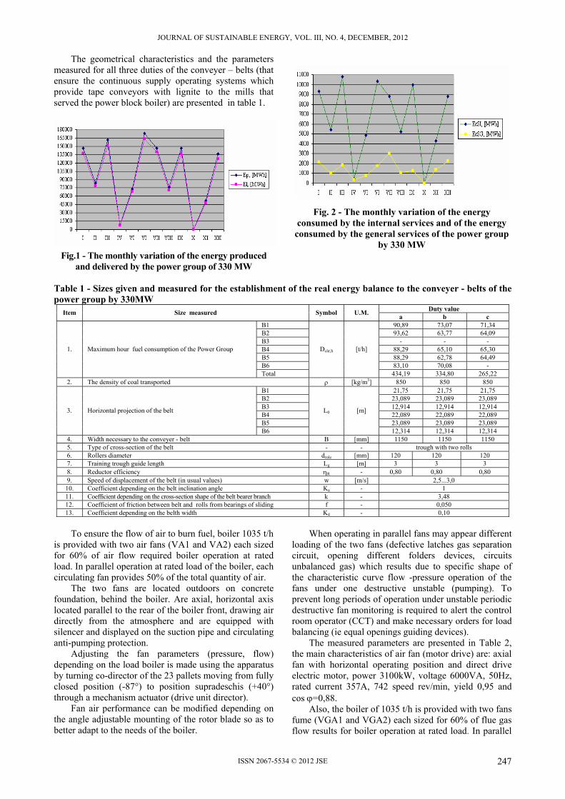
JOURNAL OF SUSTAINABLE ENERGY, VOL. III, NO. 4, DECEMBER, 2012
ISSN 2067-5534 © 2012 JSE
The geometrical characteristics and the parameters measured for all three duties of the conveyer – belts (that ensure the continuous supply operating systems which provide tape conveyors with lignite to the mills that served the power block boiler) are presented in table 1.
Fig.1 - The monthly variation of the energy produced and delivered by the power group of 330 MW
Fig. 2 - The monthly variation of the energy consumed by the internal services and of the energy
consumed by the general services of the power group by 330 MW
Table 1 - Sizes given and measured for the establishment of the real energy balance to the conveyer - belts of the power group by 330MW
Duty value Item Size measured Symbol U.M.
a b c B1 90,89 73,07 71,34 B2 93,62 63,77 64,09 B3 - - - B4 88,29 65,10 65,30 B5 88,29 62,78 64,49 B6 83,10 70,08 -
1. Maximum hour fuel consumption of the Power Group
Total
Dcăr,h [t/h]
434,19 334,80 265,22 2. The density of coal transported [kg/m3] 850 850 850
B1 21,75 21,75 21,75 B2 23,089 23,089 23,089 B3 12,914 12,914 12,914 B4 22,089 22,089 22,089 B5 23,089 23,089 23,089
3. Horizontal projection of the belt
B6
L0 [m]
12,314 12,314 12,314 4. Width necessary to the conveyer - belt B [mm] 1150 1150 1150 5. Type of cross-section of the belt - - trough with two rolls 6. Rollers diameter drole [mm] 120 120 120 7. Training trough guide length Lg [m] 3 3 3 8. Reductor efficiency R - 0,80 0,80 0,80 9. Speed of displacement of the belt (in usual values) w [m/s] 2,5...3,0 10. Coefficient depending on the belt inclination angle Ka - 1 11. Coefficient depending on the cross-section shape of the belt bearer branch k - 3,48 12. Coefficient of friction between belt and rolls from bearings of sliding f - 0,050 13. Coefficient depending on the belth width K4 - 0,10
To ensure the flow of air to burn fuel, boiler 1035 t/h is provided with two air fans (VA1 and VA2) each sized for 60% of air flow required boiler operation at rated load. In parallel operation at rated load of the boiler, each circulating fan provides 50% of the total quantity of air. The two fans are located outdoors on concrete foundation, behind the boiler. Are axial, horizontal axis located parallel to the rear of the boiler front, drawing air directly from the atmosphere and are equipped with silencer and displayed on the suction pipe and circulating anti-pumping protection. Adjusting the fan parameters (pressure, flow) depending on the load boiler is made using the apparatus by turning co-director of the 23 pallets moving from fully closed position (-87°) to position supradeschis (+40°) through a mechanism actuator (drive unit director). Fan air performance can be modified depending on the angle adjustable mounting of the rotor blade so as to better adapt to the needs of the boiler.
When operating in parallel fans may appear different loading of the two fans (defective latches gas separation circuit, opening different folders devices, circuits unbalanced gas) which results due to specific shape of the characteristic curve flow -pressure operation of the fans under one destructive unstable (pumping). To prevent long periods of operation under unstable periodic destructive fan monitoring is required to alert the control room operator (CCT) and make necessary orders for load balancing (ie equal openings guiding devices). The measured parameters are presented in Table 2, the main characteristics of air fan (motor drive) are: axial fan with horizontal operating position and direct drive electric motor, power 3100kW, voltage 6000VA, 50Hz, rated current 357A, 742 speed rev/min, yield 0,95 and cos =0,88. Also, the boiler of 1035 t/h is provided with two fans fume (VGA1 and VGA2) each sized for 60% of flue gas flow results for boiler operation at rated load. In parallel
247

JOURNAL OF SUSTAINABLE ENERGY, VOL. III, NO. 4, DECEMBER, 2012
ISSN 2067-5534 © 2012 JSE
operation at rated load of the boiler, each exhaust fan provides 50% of the total flue gas. Table 2 - Sizes measured data and drawing real power balance air fan in the group of 330 MW power
Value function under VA1 VA2 Item Size measured Symbol
a b c a b c 1. Current absorbed from mains, [A] Iabs 185,4 153,4 135,2 203,4 155,2 151,4 2. The pressure difference, [mmH2O] H (pa) 345 285 250 350 295 260 3. The coefficient of excess air 1,365 1,483 1,777 1,365 1,483 1,777 4. Moisture contained in air, [g/kg] x 10 10 10 10 10 10 5. Efficiency air fan VA 0,43 0,42 0,39 0,44 0,425 0,400 6. Performance electric motor drive em 0,92 0,90 0,88 0,93 0,91 0,90 7. Power absorbed by the motor drive, [kW] Pm,el 1695,53 1402,88 1236,43 1860,14 1419,34 1384,59 8. Yield air fan drive motor tra 0,99 0,99 0,99 0,99 0,99 0,99 9. Fuel consumption, [kg/s] Bc 121,38 93,77 74,52 121,38 93,77 74,52
10. Lower calorific value of fuel used, [kJ/kg] Hi 8206 8944 9210 8206 8944 9210
The two fans for conveying flue gases for the group are located behind electro at the rate 11,38 m, metal building located on a side of the chimney, the axis parallel to the front of the boiler. Are axial, vertical, with the suction pipe and the engine and drive the bottom discharge pipe at the top. Setting the device manager (the vortex) is a considerable improvement of the regulation
by rolling, to which has the advantage of much better performance at partial load. The measured parameters are presented in Table 3, while the main characteristics of gas fans are axial fan with vertical operating position and direct drive electric motor, power 3200kW, 6000VA voltage, frequency 50Hz, rated current 361A, speed 7600 rev/min, yield 0,95 and cos = 0,88.
Table 3 - Sizes and measured data for real electric gas fan drawing sheet of the group energy of 330 MW
Value function under VG1 VG2 Item Size measured Symbol
a b c a b c 1. Current absorbed from mains, [A] Iabs 245,2 206,8 202,3 237,20 203,20 201,60 2. The pressure difference, [mmH2O] H (pga) 225 185 185 220 180 180 3. The coefficient of excess air 1,522 1,671 2,041 1,522 1,671 2,041 4. Moisture contained in air, [g/kg] x 10 10 10 10 10 10 5. Efficiency flue gas fan VG 0,36 0,305 0,30 0,365 0,31 0,31 6. Performance electric motor drive em 0,91 0,90 0,89 0,92 0,90 0,89 7. Power absorbed by the motor drive, [kW] Pm,el 2242,41 1891,23 1850,08 2169,25 1858,31 1843,68
8. Transmission efficiency flue gas fan motor tra 0,99 0,99 0,99 0,99 0,99 0,99
9. Fuel consumption, [kg/s] Bc 121,38 93,77 74,52 121,38 93,77 74,52 10. Flue gas temperature to chimney, [C] tcoş 168,50 176,80 153,40 176,50 164,20 159,60 11. The ambient temperature, [C] tma 11,70 11,70 8,00 11,70 11,70 8,00
3. METHODOLOGY FOR ACHIEVING THE REAL ENERGY BALANCE Considering the number of drive motors for each type of consumer services in the internal part and their
specific parameters, (Table 4) could be determined hourly electricity losses in the drive motors for the three operating modes [6].
Table 4 - Nominal parameters of the motors drive consumers subject to the analysis of internal services
No. crt.
Consumer Power installed
in engine Pi, [kW]
Number of engines
Total power installed in engines
Pit, [kW]
Tated number of rotations ns,
[rot/min]
Power factor cos n
Nominal yield n, [%]
1. Exhaust fan 1 3200 1 3200 670 0,88 94,00 2. Exhaust fan 2 3200 1 3200 670 0,88 94,00 3. Air fan 1 3100 1 3100 740 0,88 91,00 4. Air fan 2 3100 1 3100 750 0,88 90,00 5. Conveyer belt type Redler -plate 1 11 1 11 1500 0,85 89,00 6. Palette knife of the conveyer belt 1 11 1 11 1500 0,85 89,00 7. Conveyer belt type Redler - craper wall 1 0,75 1 0,75 1000 0,70 71,00 8. Conveyer belt type Redler - plate 2 11 1 11 1500 0,85 89,00 9. Palette knife of the conveyer belt 2 11 1 11 1500 0,85 89,00 10. Conveyer belt type Redler - craper wall 2 0,75 1 0,75 1000 0,70 71,00 11. Conveyer belt type Redler - plate 3 11 1 11 1500 0,85 89,00 12. Palette knife of the conveyer belt 3 11 1 11 1500 0,85 89,00 13. Conveyer belt type Redler - craper wall 3 0,75 1 0,75 1000 0,70 71,00 14. Conveyer belt type Redler - plate 4 11 1 11 1500 0,85 89,00 15. Palette knife of the conveyer belt 4 11 1 11 1500 0,85 89,00 16. Conveyer belt type Redler - craper wall 4 0,75 1 0,75 1000 0,70 71,00 17. Conveyer belt type Redler - plate 5 11 1 11 1500 0,85 89,00 18. Palette knife of the conveyer belt 5 11 1 11 1500 0,85 89,00 19. Conveyer belt type Redler - craper wall 5 0,75 1 0,75 1000 0,70 71,00 20. Conveyer belt type Redler - plate 6 11 1 11 1500 0,85 89,00 21. Palette knife of the conveyer belt 6 11 1 11 1500 0,85 89,00 22. Conveyer belt type Redler - craper wall 6 0,75 1 0,75 1000 0,70 71,00
Total 12670,50 22 12670,50 - - -
248
JOURNAL OF SUSTAINABLE ENERGY, VOL. III, NO. 4, DECEMBER, 2012
ISSN 2067-5534 © 2012 JSE
Parameters determining the efficiency of conveyor belts supposes an algorithm which can be calculated using the electrical power required to drive motor Redler bands [7]. 1. Determine comsumul load of the conveyor belt with a relationship 1: sprwLKP 001 01,0 [kW] (1)
where: K0 - coefficient depending on the length of the transport band determined from the length of the conveyor belt diagrams L0 ; L0 - horizontal projection of bandwidth, [m]; w - speed of the tape, [m/s]; rsp - specific resistance, [daN/m], determined from the charts, depending on roll diameter expressed in mm. 2. Calculate power consumption horizontal laxity of the material transported, the relation 2: carDfLKP 002 003,0 [kW] (2)
where: f - friction coefficient values between 0.025 and 0.05 for roller bearings for roller bearings; Dcar - carrying capacity of the tape, [kg/s], determined by the relation 3:
2)5,0009,0(3600
1 BwkKDcar [kg/s] (3)
where: K - coefficient depending on the angle of the tape; k - coefficient determined by the branch-bearing cross-sectional shape of the strip. For three roller conveyor chute k = 4; - density of coal transported, [kg/m3]; B - width of the conveyor belt, [mm] (table 1). 3. Determine the required electrical power to be consumed to move material vertically, with the relation 4: HDP car 003,03 [kW] (4)
where: H - vertical projection of bandwidth, [m]. 4. Determine the power consumption to overcome friction between the belt conveyor and discharge chute guides, the relationship 5: gLwKP 44 [kW] (5)
where: K4 - coefficient depending on the width, the conveyors values 0.05 for B1000 mm and 0.1 mm for B>1000 mm; Lg - gutter length guide, [m]. If the system of bands analyzed, Lg = 0.
5. Calculate the electrical power needed to overcome resistance wiper strip, the relationship 6: BwP 002,05 [kW] (6)
6. Calculate the electrical power needed to overcome resistance band arresters type two drums, the relationship: carDKwKP 656 001,0 [kW] (7)
where: K5 and K6 - coefficients depend on the bandwidth. For widths of 1800 mm, K5 = 2.1, and K6 = 5.6. 7. Determine the total electric power for driving the band, the relation 8:
6
1iia PP [kW] (8)
8. Calculate the power consumption of the engine driving the relationship 9:
R
am
PP
)2,10,1( [kW] (9)
where: r=0,98 - output gear (table 1) For fans of air and gas, the balance is made using the following algorithm [2], [3], [4]: 1. Calculate the active and reactive power absorbed by engine relations 10 and 11:
mas
absnabs tg
IUP
arccos1
32
22
(10)
masabsabs tgPQ arccos (11)
where: Un – rated voltage, [V]; Iabs, cosmas – input current of the motor network, [A] (measured current) and power factor measurement. 2. Calculate the corresponding active power loss absorbed active power and active power losses varying relations 12 and13:
mas
motorabs
motormas
motorabs
PP
PP
P
masabsabsabs PPP (12)
ctabsabs PPP var (13)
249
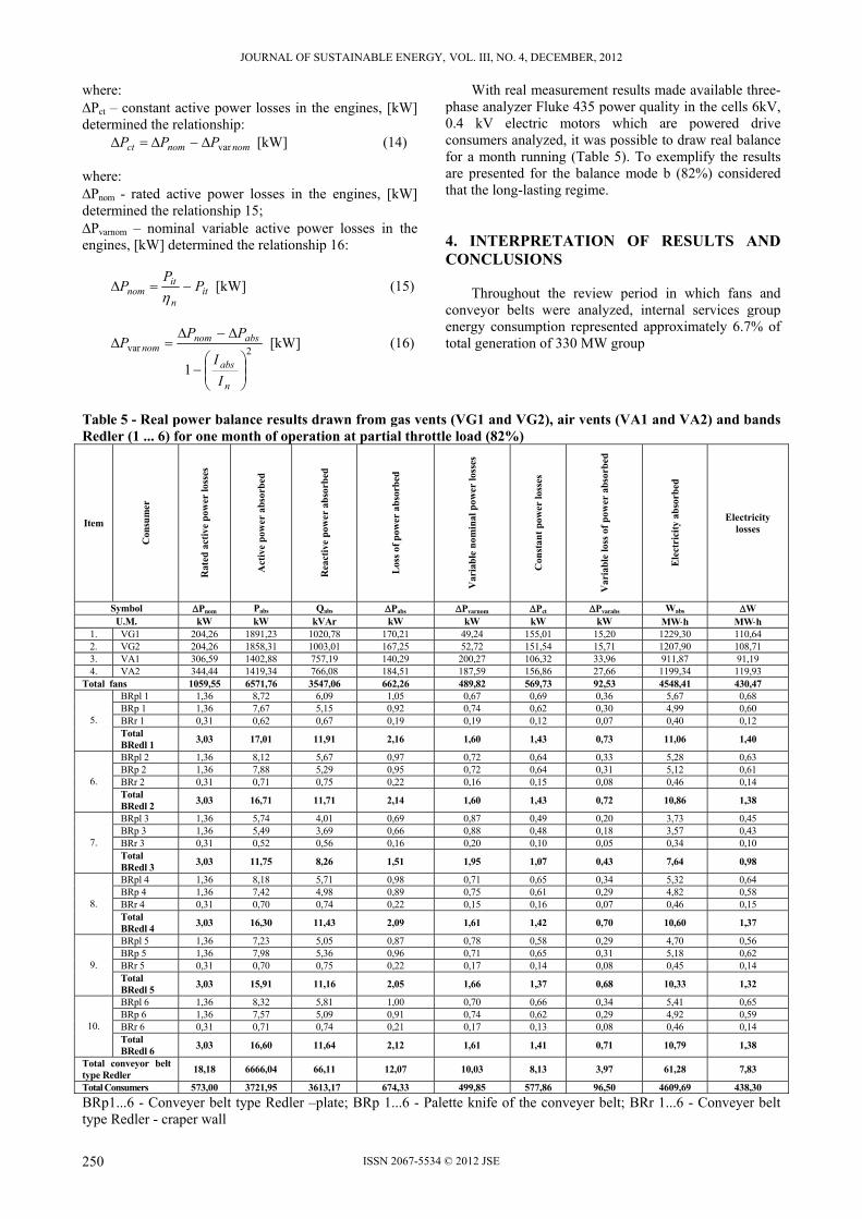
JOURNAL OF SUSTAINABLE ENERGY, VOL. III, NO. 4, DECEMBER, 2012
ISSN 2067-5534 © 2012 JSE
where: Pct – constant active power losses in the engines, [kW] determined the relationship: nomnomct PPP var [kW] (14)
where: Pnom - rated active power losses in the engines, [kW] determined the relationship 15; Pvarnom – nominal variable active power losses in the engines, [kW] determined the relationship 16:
itn
itnom P
PP
[kW] (15)
2var
1
n
abs
absnomnom
II
PPP [kW] (16)
With real measurement results made available three-phase analyzer Fluke 435 power quality in the cells 6kV, 0.4 kV electric motors which are powered drive consumers analyzed, it was possible to draw real balance for a month running (Table 5). To exemplify the results are presented for the balance mode b (82%) considered that the long-lasting regime. 4. INTERPRETATION OF RESULTS AND CONCLUSIONS Throughout the review period in which fans and conveyor belts were analyzed, internal services group energy consumption represented approximately 6.7% of total generation of 330 MW group
Table 5 - Real power balance results drawn from gas vents (VG1 and VG2), air vents (VA1 and VA2) and bands Redler (1 ... 6) for one month of operation at partial throttle load (82%)
Item
Con
sum
er
Rat
ed a
ctiv
e po
wer
loss
es
Act
ive
pow
er a
bsor
bed
Rea
ctiv
e po
wer
abs
orb
ed
Los
s of
pow
er a
bsor
bed
Var
iabl
e n
omin
al p
ower
loss
es
Con
stan
t po
wer
loss
es
Var
iabl
e lo
ss o
f p
ower
abs
orb
ed
Ele
ctri
city
abs
orb
ed
Electricity losses
Symbol Pnom Pabs Qabs Pabs Pvarnom Pct Pvarabs Wabs W U.M. kW kW kVAr kW kW kW kW MWh MWh
1. VG1 204,26 1891,23 1020,78 170,21 49,24 155,01 15,20 1229,30 110,64 2. VG2 204,26 1858,31 1003,01 167,25 52,72 151,54 15,71 1207,90 108,71 3. VA1 306,59 1402,88 757,19 140,29 200,27 106,32 33,96 911,87 91,19 4. VA2 344,44 1419,34 766,08 184,51 187,59 156,86 27,66 1199,34 119,93
Total fans 1059,55 6571,76 3547,06 662,26 489,82 569,73 92,53 4548,41 430,47 BRpl 1 1,36 8,72 6,09 1,05 0,67 0,69 0,36 5,67 0,68 BRp 1 1,36 7,67 5,15 0,92 0,74 0,62 0,30 4,99 0,60 BRr 1 0,31 0,62 0,67 0,19 0,19 0,12 0,07 0,40 0,12 5. Total BRedl 1
3,03 17,01 11,91 2,16 1,60 1,43 0,73 11,06 1,40
BRpl 2 1,36 8,12 5,67 0,97 0,72 0,64 0,33 5,28 0,63 BRp 2 1,36 7,88 5,29 0,95 0,72 0,64 0,31 5,12 0,61 BRr 2 0,31 0,71 0,75 0,22 0,16 0,15 0,08 0,46 0,14 6. Total BRedl 2
3,03 16,71 11,71 2,14 1,60 1,43 0,72 10,86 1,38
BRpl 3 1,36 5,74 4,01 0,69 0,87 0,49 0,20 3,73 0,45 BRp 3 1,36 5,49 3,69 0,66 0,88 0,48 0,18 3,57 0,43 BRr 3 0,31 0,52 0,56 0,16 0,20 0,10 0,05 0,34 0,10 7. Total BRedl 3
3,03 11,75 8,26 1,51 1,95 1,07 0,43 7,64 0,98
BRpl 4 1,36 8,18 5,71 0,98 0,71 0,65 0,34 5,32 0,64 BRp 4 1,36 7,42 4,98 0,89 0,75 0,61 0,29 4,82 0,58 BRr 4 0,31 0,70 0,74 0,22 0,15 0,16 0,07 0,46 0,15 8. Total BRedl 4
3,03 16,30 11,43 2,09 1,61 1,42 0,70 10,60 1,37
BRpl 5 1,36 7,23 5,05 0,87 0,78 0,58 0,29 4,70 0,56 BRp 5 1,36 7,98 5,36 0,96 0,71 0,65 0,31 5,18 0,62 BRr 5 0,31 0,70 0,75 0,22 0,17 0,14 0,08 0,45 0,14 9. Total BRedl 5
3,03 15,91 11,16 2,05 1,66 1,37 0,68 10,33 1,32
BRpl 6 1,36 8,32 5,81 1,00 0,70 0,66 0,34 5,41 0,65 BRp 6 1,36 7,57 5,09 0,91 0,74 0,62 0,29 4,92 0,59 BRr 6 0,31 0,71 0,74 0,21 0,17 0,13 0,08 0,46 0,14 10. Total BRedl 6
3,03 16,60 11,64 2,12 1,61 1,41 0,71 10,79 1,38
Total conveyor belt type Redler
18,18 6666,04 66,11 12,07 10,03 8,13 3,97 61,28 7,83
Total Consumers 573,00 3721,95 3613,17 674,33 499,85 577,86 96,50 4609,69 438,30
BRp1...6 - Conveyer belt type Redler –plate; BRp 1...6 - Palette knife of the conveyer belt; BRr 1...6 - Conveyer belt type Redler - craper wall
250

JOURNAL OF SUSTAINABLE ENERGY, VOL. III, NO. 4, DECEMBER, 2012
ISSN 2067-5534 © 2012 JSE
Of the total domestic consumption of electricity services for the month of study, analysis equipment consumption is about 42.80% and the total energy produced by energy group, representing about 2.86%. The category also includes internal service users mills whose coal consumption is about 1.50% and various pumping plants whose consumption is approximately (1.2 ... 1.3)% of total energy produced by energy group. Related to the consumption of the proper functioning of equipment and installations for domestic services for the proper conduct of the real energy balance should be added and energy loss associated electrical cables through which these facilities/equipment are supplied from the network and not least energy losses in transformers internal services. Overall, bands Redler works in all three regimes of charge energy group, with yields around 87.20%. Electricity consumption of the bands of course vary depending Redler hourly fuel consumption of coal transported group and density, leading to variations in power drive motor and hence the variation of absorbed power and electricity network. Given the technological and constructive characteristics, air vents are characterized by low values of power technology, under the project, ranging from the three operating modes, between 34% and 39.87% for fan air VA1, respectively 35.80% and 40.61% for VA2 air fan. Also, gas vents are characterized by low values of functional technological powers, under the project, between 26.53% and 32.57% for VG1 gas fan and between 27.24% and 33.07% for VG2 gas fan. In general, high values are due to losses in fan motors drive them but, characteristics of the working fluid (air or flue gas). Given the energy balance results presented above, it is necessary to take technical measures - economic and organizational help to the improvement of balance and power consumption savings [1], [5], [8]. The main measures aimed at: ensuring optimal functioning (at full load) technological equipment and avoid possible operation group at low loads, revisions and repairs after the schedule and quality, requiring the
tracking and highlighting proper lifetime of the equipment and equipment, reducing load losses especially at low voltage consumers, periodic cleaning of the fans and capacitors, as deposits affect engine load, learning to use the variable speed drives to consumers of 6 kV and 0.4 kV and especially the bands and fans Redler Following the implementation of these measures, in one year, for example, regime b (presented in detail throughout the paper), with an average of 5,000 unit operating hours, the amount of energy saved from internal services is 271.90 MWh/year, so about 9516.50 Euro/year. Acknowledgment “This work was partially supported by the strategic grant POSDRU/CPP107/DMI1.5/S/78421, Project ID 78421 (2010), co-financed by the European Social Fund – Investing in People, within the Sectoral Operational Programme Human Resources Development 2007-2013.” BIBLIOGRAPHY [1]. Mereuţă, C., Măsuri practice generale pentru economisirea
energiei electrice în industrie, Editura Tehnică, Bucureşti, 1985.
[2]. Carabogdan, I. Gh., ş.a., Bilanţuri energetice. Probleme şi aplicaţii pentru ingineri, Editura Tehnică, Bucureşti, 1986.
[3]. ***, Normativul pentru întocmirea şi analiza bilanţurilor energetice. PE 902/1996, Bucureşti, CIDE.
[4]. ***, Normativ privind metodica de întocmire şi analiza bilanţurilor energetice în întreprinderile industriale, ICEMENERG, Bucureşti, 2000.
[5]. Răducanu, C., ş.a., Audit energetic, Editura Agir, Bucureşti, 2000.
[6]. Ionescu, C. D., ş.a., Monitorizarea şi evaluarea continuă a eficienţei energetice, Editura Agir, Bucureşti, 2001.
[7]. Mircea, I., Ruieneanu, L., Dinu, R.C., Producerea energiei electrice şi termice, Îndrumar de laborator, vol.I, Reprografia Universităţii din Craiova, 2001.
[8]. Vuc, Gh., Managementul energiei electrice, Editura Agir, Bucureşti, 2001.
251

JOURNAL OF SUSTAINABLE ENERGY, VOL. III, NO. 4, DECEMBER, 2012
ISSN 2067-5534 © 2012 JSE
VARIATION OF ELECTRICAL PARAMETERS OF TWO PUBLIC LIGHTING SOLUTIONS DUE TO CONTINUOUS DIMMING OF
LIGHT OUTPUT
VASILIU R.B., CHINDRIŞ M., CZIKER A., GHEORGHE D.
Technical University of Cluj – Napoca [email protected], [email protected],
Abstract: Public lighting applications, including street and pedestrian lighting provide crucial services for human safety, productivity and comfort in the modern urban and suburban landscape. However, energy charges for these lighting applications represent the largest part of all expenses for public lighting. The increasing price of electricity is, by itself, responsible for the majority of the increase in streetlight operation budgets. Telemanagement systems that control public lighting networks offer a significant opportunity to save energy and decrease the impact of artificial lighting on the environment. When high intensity discharge lamps are used regulation of light flux can be achieved using either step-dimming or continuous dimming ballasts (1-10V, DALI). This paper presents the variation of electrical parameters of two lighting solutions due to continuous dimming of light output. The first solution consists of a high pressure sodium SON-T 150W lamp and the electronic DynaVision SON ballast. The ceramic metal halide CDO-TT 150W lamp and the electronic DynaVision CDO ballast represent the second studied solution. Both solutions use the 1-10V analogic protocol technology for continuous dimming of lamp light flux. The results are presented as a comparison of the influence of light output dimming on the electrical parameters of the two solutions. This comparison is defined in terms of active and reactive power consumption, current harmonics and power factor values.
Key words: Electrical parameters, continuous dimming, light output, public lighting
1. INTRODUCTION
Modern public lighting provides many benefits to
the community both in terms of safety and security of the citizens, as well as economically. Public safety involves reducing road accidents at night and reductions in street crime and the fear of it. Also by highlighting architectural assemblies using proper
lighting techniques, the city can become an attraction for many visitors leading to tourism development.
Globally an estimated 218 TWh of electricity was consumed by outdoor lighting in 2005, amounting to about 8% of total lighting electricity consumption. From this, street and roadway lighting used about 114 TWh of energy globally while illumination of car parks is responsible for the consumption of 88 TWh of electricity in the same year [1].
In Europe there are 80 million street lights consuming about 60 TWh per year. According to some European Initiatives like the European project “E-street” 63.7% or 38 TWh of energy consumption in outdoor lighting could be saved by implementing intelligent systems like adaptive street lighting and the use of LEDs [2]. 2. TELEMANAGEMENT SYSTEMS AND LIGHT OUTPUT DIMMING
Currently street lighting control systems range from simple to complex structures. In order to describe these control systems different terms have been used over the years such as telemanagement, adaptive, dynamic and intelligent.
A telemanagement system enables the lighting system to automatically react to external parameters like traffic density, remaining daylight level, road constructions, accidents or weather circumstances. The operating costs of public lighting systems can be lowered if the critical data needed to make better planning and operation decisions can be cost effectively collected. However this design can be implemented only using a suitable network that can gather the information and can exercise control. Today power line based communication networking can achieve significant operating and energy cost savings while improving both the reliability and the quality of public lighting systems [3].
Maintaining the same illumination intensity for a pre-defined period is not an optimal solution. There is no need for the same light intensity if there is very little traffic and a clear sky. Regulation of the light level by dimming the light output of the lamp based on
252

JOURNAL OF SUSTAINABLE ENERGY, VOL. III, NO. 4, DECEMBER, 2012
ISSN 2067-5534 © 2012 JSE
the desired situation is the main function of any telemanagement system.
High intensity discharge lamps can be dimmed using either step-dimming or continuous dimming technologies. When electronic ballasts are used the dimming level is set by an external module that communicates with the ballast’s control interface. The main control interfaces are 1-10V, DALI and proprietary interfaces.
Ballasts with 1-10V input dim the light output according to the voltage level of there set point input in a range of 1-10 volts, where 10 volts means maximum level and 1 volt means minimum level [3]. To switch the light on and off the power to the ballasts is interrupted using a relay. 3. ANALYSIS OF THE MEASUREMENTS RESULTS
The increasing use of non-linear equipment (electronic power converters, discharge-type lighting, etc.) in electrical distribution systems has raised the level of concern about the effects of these loads on the system [4].
From the point of view of lighting equipments of special concern are single-phase devices with rectifier front-end power supplies (electronic lighting ballast) and discharge lamps.
This study analysis two lighting solutions used nowadays in public lighting applications. The first solution consists of a high pressure sodium SON-T 150W lamp and the DynaVision SON 1-10V electronic ballast. The ceramic metal halide CDO-TT 150W lamp and the electronic DynaVision CDO ballast represent the second studied solution. Both solutions use the 1-10V analogic protocol technology for continuous dimming of lamp light flux.
The high pressure sodium lamps are very energy efficient and last up to four eyes. The lamp is optically efficient but has a long run-up time. Also it has limited color rendering and provides a orange/yellow light. Metal halide lamps are based on newer technology and trends in public lighting. They are energy efficient and provide a high quality white light. These lamp types offer significant environmental advantages because of very low mercury levels and high energy efficiency [5].
The 1-10V electronic ballasts used are controllable ballasts that expect an external signal to switch or set a dim level.
In order to determine the variation of electrical parameters for the studied solution, a series of measurements were conducted. These measurements also help to recognize the problems that these equipments cause to its electrical environment surrounding in different working regimes due to continuous dimming of light output. The experimental setup is presented in figure 1.
Fig.1 - Experimental setup
The setup consists of a Fluke 43 power quality analyzer (used for the analysis of single-phase systems), an autotransformer, a PC station, a constant voltage source and the SON and CDO solutions. Also a luxmeter was used to determine the relation between the light level and power level at different values of the control voltage. Figure 2 presents the experimental setup scheme.
Fig.2 - Experimental setup scheme
A series of 20 measurements were made for each solution by lowering the DC control voltage by 0.5V steps using the constant voltage source. Table 1 presents the RMS values of the current fundamental as well as the level γk of the main current harmonics for the two studied solutions related to voltage control, while the waveforms and harmonic current analysis are presented in figures 3, 4, 5 and 6.
253

JOURNAL OF SUSTAINABLE ENERGY, VOL. III, NO. 4, DECEMBER, 2012
ISSN 2067-5534 © 2012 JSE
Table 1 - The level of current harmonics related to the value of the control voltage SON-T solution CDO-TT solution DC control
voltage [V] I1 [mA] γ3 [%] γ5 [%] γ7 [%] I1 [mA] γ3 [%] γ5 [%] γ7 [%] 10 701 7 4 2 702 7 5 2 9.5 704 8 5 1 703 7 5 1 9 694 7 5 1 684 7 6 2
8.5 670 8 5 1 663 7 6 1 8 645 8 4 2 643 8 6 1
7.5 617 8 5 2 616 8 6 1
7 590 8 5 2 588 8 6 2
6.5 565 8 5 2 554 8 6 2
6 531 9 5 2 521 9 6 2
5.5 500 9 6 2 489 9 6 2
5 466 10 6 2 460 9 6 2
4.5 434 10 6 3 418 10 6 2
4 424 10 6 3 388 11 7 2
3.5 420 10 6 2 359 12 7 2
3 411 10 7 2 325 13 8 2
2.5 404 10 7 2 291 13 8 2
2 400 11 7 2 256 15 9 3
1.5 398 11 6 3 222 17 10 3
1 391 12 6 3 223 17 10 2
Fig.3 - Harmonic current analysis (Ucontrol = 10 V) : left – SON-T solution; right – CDO-TT solution
Fig.4 - Waveforms (Ucontrol = 10 V, 1 – Supply voltage, 2 – Input current) :
left – SON-T solution; right – CDO-TT solution
254

JOURNAL OF SUSTAINABLE ENERGY, VOL. III, NO. 4, DECEMBER, 2012
ISSN 2067-5534 © 2012 JSE
Fig.5 - Harmonic current analysis (Ucontrol = 1 V): left – SON-T solution; right – CDO-TT solution
Fig.6 - Waveforms (Ucontrol = 1 V, 1 – Supply voltage, 2 – Input current) :
left – SON-T solution; right – CDO-TT solution
As it can be observed the current harmonic spectrums reveal a low-harmonic content. In the case of the first solution the level of the 3rd harmonic is between 7-12%, the level of the 5th is between 4-7% while the level of the 7th harmonic is between 1-3% of the fundamental over the 1-10V control voltage interval. Measurements result for the second solution have shown that the level of the 3rd harmonic is between 7-17%, the level of the 5th harmonic is between 5-10% while the level of the 7th harmonic is between 1-3% of the fundamental over the 1-10V control voltage interval.
The parameter that best quantifies the harmonic pollution introduced by these lighting solutions is the current harmonic distortion factor (THD). Figure 7 presents the variation of the values of current distortion factor over the 1-10V control voltage interval. The values obtained are between 9-13.5 % in the case of the SON solution, 9% corresponding to the maximum control voltage (10V) while a value of 13.5% for the THD was obtained for the minimum control voltage (1V). In the case of the CDO solution these values ranged between 9.3% (10V) to 19.8% (1V).
5
7
9
11
13
15
17
19
21
10 9 8 7 6 5 4 3 2 1
Ucontrol [V]
TH
Di
[%]
Son solution
CDO solution
Fig.7 - Variation of current THD
The variation of power factor was also studied.
Figure 8 presents the results of the measurements over the 1-10V range.
0.88
0.9
0.92
0.94
0.96
0.98
1
10 9 8 7 6 5 4 3 2 1
Ucontrol [V]
PF SON solution
CDO solution
Fig.8 - Variation of power factor
255
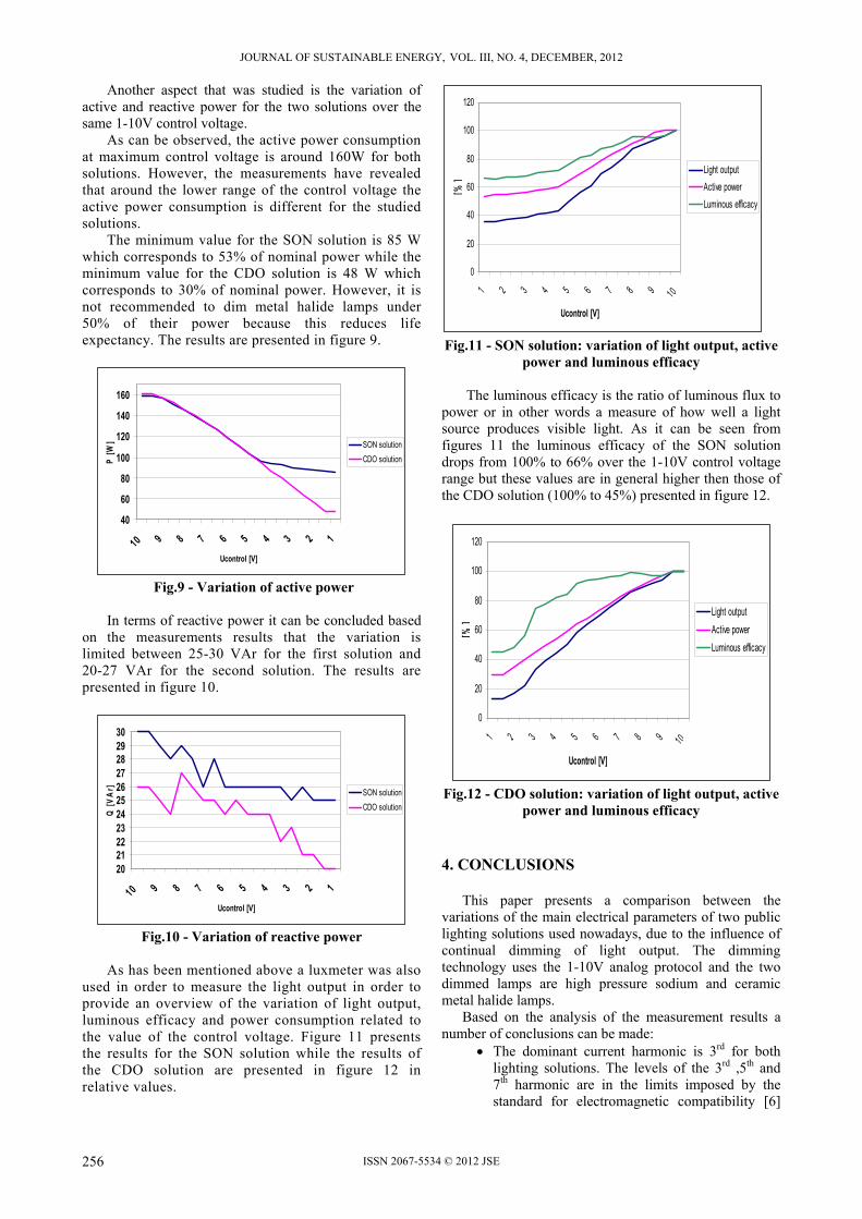
JOURNAL OF SUSTAINABLE ENERGY, VOL. III, NO. 4, DECEMBER, 2012
ISSN 2067-5534 © 2012 JSE
Another aspect that was studied is the variation of active and reactive power for the two solutions over the same 1-10V control voltage.
As can be observed, the active power consumption at maximum control voltage is around 160W for both solutions. However, the measurements have revealed that around the lower range of the control voltage the active power consumption is different for the studied solutions.
The minimum value for the SON solution is 85 W which corresponds to 53% of nominal power while the minimum value for the CDO solution is 48 W which corresponds to 30% of nominal power. However, it is not recommended to dim metal halide lamps under 50% of their power because this reduces life expectancy. The results are presented in figure 9.
40
60
80
100
120
140
160
10 9 8 7 6 5 4 3 2 1
Ucontrol [V]
P [
W] SON solution
CDO solution
Fig.9 - Variation of active power
In terms of reactive power it can be concluded based
on the measurements results that the variation is limited between 25-30 VAr for the first solution and 20-27 VAr for the second solution. The results are presented in figure 10.
2021222324252627282930
10 9 8 7 6 5 4 3 2 1
Ucontrol [V]
Q [
VA
r] SON solution
CDO solution
Fig.10 - Variation of reactive power
As has been mentioned above a luxmeter was also
used in order to measure the light output in order to provide an overview of the variation of light output, luminous efficacy and power consumption related to the value of the control voltage. Figure 11 presents the results for the SON solution while the results of the CDO solution are presented in figure 12 in relative values.
0
20
40
60
80
100
120
1 2 3 4 5 6 7 8 9 10
Ucontrol [V]
[%]
Light output
Active power
Luminous efficacy
Fig.11 - SON solution: variation of light output, active
power and luminous efficacy
The luminous efficacy is the ratio of luminous flux to power or in other words a measure of how well a light source produces visible light. As it can be seen from figures 11 the luminous efficacy of the SON solution drops from 100% to 66% over the 1-10V control voltage range but these values are in general higher then those of the CDO solution (100% to 45%) presented in figure 12.
0
20
40
60
80
100
120
1 2 3 4 5 6 7 8 9 10
Ucontrol [V]
[%]
Light output
Active power
Luminous efficacy
Fig.12 - CDO solution: variation of light output, active
power and luminous efficacy 4. CONCLUSIONS
This paper presents a comparison between the variations of the main electrical parameters of two public lighting solutions used nowadays, due to the influence of continual dimming of light output. The dimming technology uses the 1-10V analog protocol and the two dimmed lamps are high pressure sodium and ceramic metal halide lamps.
Based on the analysis of the measurement results a number of conclusions can be made:
The dominant current harmonic is 3rd for both lighting solutions. The levels of the 3rd ,5th and 7th harmonic are in the limits imposed by the standard for electromagnetic compatibility [6]
256

JOURNAL OF SUSTAINABLE ENERGY, VOL. III, NO. 4, DECEMBER, 2012
ISSN 2067-5534 © 2012 JSE
for lighting equipments (class C) over the entire 1-10V dimming range;
The current harmonic distortion factor (THD) varies between 9% (minimum for both solutions) to the maximum value of 13.5% for the SON solution and approximately 20% for the CDO solution.
In terms of power factor variation it was observed that the SON solution presents a higher power factor then the CDO solution in the lower part of the control voltage range. In both cases a relation can be made between the lower values of the power factor and the increasing values of current harmonic distortion factor. This is due harmonic pollution introduced by these equipments;
The active power consumption drops almost linear in both cases related to the control voltage with an advantage for the CDO solution (down to 30% of active power). However lamp manufacturers do not recommend and do not guarantee the proper function of metal halide lamps when dimmed under 50% of power. Variation of reactive power consumption is insignificant in both cases;
From the point of view of luminous efficacy, as a parameter of energy efficiency, it can be concluded based on the results obtained from the measurements that the CDO solution is more efficient in the 2.5-10V control voltage range. Under this value the luminous efficacy of this solution drops drastically and the SON solution is more efficient.
Acknowledgment This paper was supported by the project “Doctoral studies in engineering sciences for developing the knowledge based society-SIDOC” contract no. POSDRU/88/1.5/S/60078, project co-funded from European Social Fund through Sectorial Operational Program Human Resources 2007-2013. REFERENCES [1]. International Energy Agency, Light’s Labour’s lost, (61
2005 27 I PI), 2006, ISBN: 92641095IX. [2]. http://www.esoli.org [3]. Walraven, H., Work Package 2: Market Assessment and
Review of Energy Savings, E-street Initiative, July 2006, www.e-streetlight.com.
[4]. Chindriş, M., Ştefanescu, S., Cziker, A., Neutral currents in electrical systems supplying lighting networks, The 2nd International Lighting Conference, Cluj-Napoca, Romania, 8-9 May 2003.
[5]. E-street, Project Report – Intelligent Road and Street lighting in Europe, E-street Initiative, August 2008, www.e-streetlight.com.
[6]. IEC 61000-3-2: 2001, Electromagnetic compatibility, Part 3: Limits – Section 2: Limits for harmonic current emissions (equipment input current up to and including 16 A per phase).
[7]. D.V., Brajovic, D.D., Sretenovic, „Influence of continual regulation of light flux in public lighting on electric energy quality”, 15th International Research/Expert Conference „Trends in the Development of Machinery and Associated Technology”, TMT 2011, Prague, Czech Republic, 12-18 September 2011.
257

JOURNAL OF SUSTAINABLE ENERGY, VOL. III, NO. 4, DECEMBER, 2012
ISSN 2067-5534 © 2012 JSE
HYBRID GREY FORECASTING MODEL FOR IRAN’S ENERGY CONSUMPTION AND SUPPLY
HAMIDREZA M., SHAGHAYEGH K.
Department of Statistics, Tehran North Branch, Islamic Azad University, Tehran, Iran [email protected], [email protected]
Abstract - Grey theory deals with system that are characterized by poor information or for which information is lacking. This study presents an improved grey GM (1, 1) model, using a technique that combines residual modification with Markov Chain model. We use energy consumption and supply of Iran to test the accuracy of proposed model. The results show that the Markov Chain residual modification model achieves reliable and precise results. Keywords: Grey Forecasting Model; Markov Chain; Energy System 1. INTRODUCTION
In recent years, grey system theory has become a very useful method of solving uncertainty in problems under discrete data and incomplete information. Deng [4] proposed that the Grey theory concerns with the grey generation, relation analysis, model construction, prediction, decision – making and system control.
Most of the prediction methods require a large number history data and will make use of statistical method to analyze the properties of the system. The statistical predictors may not provide satisfied results owing to the increasing complexity of real-word problems. Furthermore because of additional noise from outside and the complex interrelation among the system or between the system and its environment, it is more difficult to analyze the system. Therefore, methods such as neural network, fuzzy system and grey models are proposed to increase the prediction accuracy. As a prediction model, the grey dynamic model has the advantages of setting up a model with few data.
GM (1, 1) type of grey model is the most widely used in the literature known as Grey Model First Order one Variable. This model is a time series for forecasting model. The differential equations of the GM (1, 1) model have time-varying coefficients. In other words, the model is renewed as the new data become available to the prediction model. This model is easy to understand and simple to calculate with acceptable accuracy, also lack of flexibility to adjust the model to achieve higher forecasting precision. Therefore, researchers begin to shift their attention to find the hybrid Grey model, Grey Markov, Grey Fourier, Grey Fuzzy, etc. Su and Chen[1], proposed an improved grey forecasting model that combines residual modification and residual artificial
neural network sign estimation to forecast power demand. Lee and Ton [7], proposed an approach that combines residual modification and residual genetic programming sign estimation to improve the precision of the residual sign estimator. Y. Hsu and et al [6], proposed Markov-Fourier grey model prediction approach to predict the turning time of Taiwan weighted stock index for increasing the forecasting accuracy. Lc. Hsu [5], modified the residual of GM (1, 1) model and accepted Markov-Chain sign estimation to forecast the value of the global integrated circuit industry. C. Yidong and S. Hanlin [3] introduced metabolic grey model together with the residual GM (1, 1) model. C. Sun and G. Lin [2], applied hybrid Grey Forecasting model for Taiwan's Hsinchu science industrial park. Sh. Kordnoori and H. Mostafaei [8] applied the grey markov model for predicting the iran’s oil production and export. The framework of our research study is as follow:
2. RESEARCH METHODOLOGY This section introduces how to establish the mathematical model. A. To establish GM (1, 1) Assume an original data series to be
The Accumulated Generation Operation (AGO) is
expressed as
(1)
The first – order differential equation of GM (1, 1) model
is then give as
258

JOURNAL OF SUSTAINABLE ENERGY, VOL. III, NO. 4, DECEMBER, 2012
ISSN 2067-5534 © 2012 JSE
(2)
The solution for (2) is
(3)
Where and the coefficients a andb
are called developing and grey input coefficient,
respectively. By least-square method, they can be
obtained as
(4)
Where
(5)
(6)
B. Markov Residual Modified Grey Model
(MRMGM)
Residual errors of Grey Model are obtained using Markov Chain. Markov Chain predicts the future development according to the transition probability among states, which reflects the internal law of all states. Therefore, markov method can be used for predicting of the system with high fluctuation. Define residual series
as
(7)
Where , k=2, 3, … , n.
Denote absolute values of residual series as as
(8)
Where .
AGM (1, 1) model of can be established as
(9)
Where are estimated using OLS. Assume that sign of kth data residual is in state 1 when it is positive and in state 2 when it is negative. A one step transition probability P is associated with each possible transition from state i to state j , and P can be estimated
using means the number
of years whose residuals are state i , and is number of transitions from state i to state j that have occurred.
These Values can be denoted as a transition matrix
R:
(10)
Denote the initial state distribution by the
vector , where and
are the transition possibility of state1 and state2. Set the
nth data to be the initial state, and state transition
possibility vector to be . Calculation of the state
possibility vector of (i+1) th step transformation after
initial state is as follow:
(11)
Where are k th step residual state probabilities.
Let the sign of the k step residual be represented as
follows:
(12)
259

JOURNAL OF SUSTAINABLE ENERGY, VOL. III, NO. 4, DECEMBER, 2012
ISSN 2067-5534 © 2012 JSE
An improved Grey model with residual modification and
Markov Chain sign estimation can be formulated as
(13)
Where 1) and
C. Error Analysis To investigate the accuracy of forecasting models,
comparison of forecasting results can be calculated.
Relative Percentage Error (RPE) compares real and
forecast values as
(14)
3. APPLICATIONS
Energy is an essential source of economic
development. Therefore, many countries are concerned with energy–related issues. Energy consumption is an influential economic index, which reflects the industrial development of a country.
In the recent 30 years, the studies on energy system forecasting models have already made great progress, and many forecasting models have been developed. Forecasting energy consumption by common statistical methods usually needs the making of assumptions such as the normal distribution of energy consumption data or a large sample size. However, the data of energy consumption are often very few or non normal. As a grey forecasting model can be formed for at least four date points or ambiguity data, it can be adopted to forecast energy consumption. To minimize the errors of grey forecasting model, we develop an improved grey forecasting model.
Iran ranks among the worlds top tree holders of both proven oil and natural gas reserves. It is one of the leading members of OPEC (Organization of Petroleum Exporting Countries) and the Organization of Gas Exporting Countries (GECF).
To demonstrate the effectiveness of the proposed grey forecasting model, the real case of total energy consumption and supply of Iran are considered as examples. The annual total energy consumption and supply of Iran from 1992 to 2006 are employed as the model – fitting and the data for 2007 and 2008 are utilized as expose testing. The data of this work are listed in table 1, provided by ministry of energy [9].
Table 1 - Total energy consumption and supply of Iran from 1992 to 2006. Year 1992 1993 1994 1995 1996 Total energy consumption
496.2 512.3 559.6 561.6 625.2
Energy Supply
630.5 672.4 736.5 771.0 827.1
Year 1997 1998 1999 2000 2001 Total energy consumption
658 680.9 695.2 683.2 682.8
Energy Supply
865.5 897.6 929.6 923.1 933.7
Year 2002 2003 2004 2005 2006 Total energy consumption
730.7 768.4 831.0 903.2 998.9
Energy Supply
999.0 1056.3 1136.0 1239.1 1353.1
Now we are applying the proposed model to forecast the total energy consumption and supply. From the data in table 1 and the GM (1, 1) model, we obtain:
(Total Energy Consumption)
(Energy Supply) The absolute values of residual series are:
8.06072, 15.62665, 7.05747, 30.73832, 36.56317, 31.26396, 16.08515, 26.73134, 59.34620, 45.12289, 42.62774, 16.83010, 16.89755, 72.37941 (Total Energy Consumption)
14.53580, 16.23958, 15.79832, 35.26199, 35.24836, 27.07121, 16.84013, 33.93966, 69.76756, 53.14776, 46.88953, 20.70744, 26.27839, 81.54200 (Energy Supply)
The Markov Residual Modified Grey Models (MRMGM) is:
(Total Energy Consumption)
(Energy Supply) As comparing with GM (1, 1) model, the forecast values of 2007 and 2008 by these two methods are listed in table 2 and 3. Table 2 - The forecast result compared with GM (1, 1) model Years Actual total
energy consumption
GM(1,1) model forecast precision value
MRMGM Forecast value precision
2007 1084.0 968.56 89.35 1001.382 92.38 2008 1115.1 1012.601 90.80 1045.601 93.77
Table 3 - The comparison between GM (1, 1) and MRMGM Years
Actual energy supply
GM(1,1) model forecast precision value
MRMGM Forecast Value precision
2007 1453.7 1333.349 91.72 1364.079 93.83 2008 1493.1 1398.033 93.63 1431.196 95.85
Table 2 and 3 show a better precision obtained by the markov residual modified grey model. Finally we predict the total energy consumption and supply from, 2009 to 2021 by MRMGM. The forecasted values are listed in table 4.
260

JOURNAL OF SUSTAINABLE ENERGY, VOL. III, NO. 4, DECEMBER, 2012
ISSN 2067-5534 © 2012 JSE
Table 4 The predicted values by MRMGM. Year Total energy
consumption Energy supply
2009 2010 2011 2012 2013 2014 2015 2016 2017 2018 2019 2020 2021
1091.815 1140.117 1190.601 1243.365 1298.513 1365.154 1416.900 1479.368 1595.184 1613.975 1685.877 1761.031 1839.585
1501.641 1575.586 1653.204 1734.682 1820.213 1910.003 2004.266 2103.230 2207.131 2319.220 2430.762 2551.033 2677.324
4. CONCLUSION The original GM (1, 1) model is a model with a group of differential equations adapted for variance of parameters. In this article, we have applied an improved grey GM (1, 1) model by using a Markov Residual Modified Grey Model. Using the data of total energy consumption and supply of Iran from 1992 to 2006, we concluded that the Markov Chain residual modification model achieves results with higher precisions than the original GM(1, 1) model. Finally, we predicted the total energy consumption and energy supply of Iran from 2009 to 2021 by MRMGM.
REFERENCES [1]. Cc. Hsu, Cy. Chen. Applications of improved grey prediction model for power demand forecasting. Energy converse manage; 44(14), 2003, pg.1141-90. [2]. Chia Chi Sun and Grace T R Lin. Hybrid Grey Forecasting model for Taiwan's Hsinchu Science Industrial Park. Journal of Scientific & Industrial Research, 68, 2009, pg. 354-360. [3]. CUI Yidong and Sun Hanlin. Periodicity Impact on the accuracy in Grey model based internet traffic prediction. Chinese journal of electronics, 19(1), 2010. [4]. JL. Deng. Grey System Fundamental method. Wuhan China: Huazhing University of Science and Technology,1982. [5]. Li-Chang Hsu. Applying the grey prediction model to the global integrated circuit industry. Technological forecasting & Social change; 70(6),2003, pg. 563-574. [6]. Yen-Tseng Hsu.Ming-Chung Liu, Jerome Yeh, Hui-Fen Hung. Forecasting the turning time of stock market based on Markov-Fourier grey model. Expert Systems with applications,36, 2009, pg. 8597-8603. [7]. Yi-Shian Lee, Lee-Ing Ton. Forecasting energy consumption using a grey model improved by incorporation genetic programming. Energy conversion and Management 52, 2011, pg. 147-152. [8]. Shaghayegh Kordnoori, Hamidreza Mostafaei. Grey Markov model for predicting the crud oil production and export in Iran, 3(2),2011, pg. 1029-1033. [9]. http://pep.moe.org.ir/.
261

JOURNAL OF SUSTAINABLE ENERGY, VOL. III, NO. 4, DECEMBER, 2012
ISSN 2067-5534 © 2012 JSE
STOCHASTIC ANALYSIS UPON THE FEASIBILITY OF THE GEOTHERMAL ENERGY EXPLOITATION
FELEA. I., PANEA C. University of Oradea, Department of Energy Engineering Universităţii no.1, Oradea,
[email protected] Abstract - Geothermal resources are included in the category of regenerative energetic resources, which through a real exploitation can assure the satisfying desideratum of long living development under energetic aspect. Considering the fact that the measurements used for evaluating the feasibility indicators of the geothermal energy efficiency have a random character, the stochastic treatment of these evaluations is legitimate. In the paper, after a short justification on the utility of the concern, there is presented the evaluation methodology in stochastic way upon the GEES feasibility and a case study. The final part comprises the conclusions of the analysis.
Keywords: geothermal energy, exploitation, feasibility, stochastic analysis. 1. INTRODUCTION
The long lasting energetic resources rationally
exploited [1, 2] can be enclosed in the category of the regenerative energetic resources and are vised by the E.U Directive 2009/28/CE through which the following fundamental acomplisments are to be reached until 2020: Through use reduction of the fosil combustible,
to assure the decrease with 20% of the greenhouse gases emissions;
The increase with 20% of regenerable energies sources (RES) within the total energetic consumption of the E.U., as well as a 10% target of biofuel in the energetic consumption for transportation;
Through the improvement of energetic efficiency, a reduction with 20% of the primary energy consumption up against the level at which the consumption might have reached without these measurements. Furthermore E.U proposes that the level of emissions to be reduced up to 30%, with the condition that the other developed states would adopt similar objectives, these being included in a future global environment agreement post 2012. Negotiations in this direction within the United Nations are still in progress.
The exploitation systems of hidrogeothermal resources are oriented on the following main directions, applied according to the energetic potential of the deposit:
Direct exploitation ≡ thermic energy extraction ;
Indirect exploitation ≡ thermo – mechano – electric conversion;
Combined exploitation (thermic and electric energy);
Complex exploitation ( energy with balneology and biologic purpose);
Applied solutions, nowadays, for the geothermal energy exploitation systems (GEES) are various [3÷7]. The projects for geothermal energy exploitation are analysed in comparison with other regenerative energetic resources, on the basis of some established feasibility criteria [2,8] in which is often operated with fixed values of the operand: investment expenses, exploitation and incomes from produced energy exploitation expenses. In the present paper it is justified the use of random variable values for the operand, the methodology being named and also exemplified the method of work for this case. 2. THE ANALYSIS METHODOLOGY
The criteria and feasibility indicators applied for GEES are [8,9]:
a. The simple way of reclaiming the investment
It is an indicator that compares the value of the necessary investments for GEES accomplishment with the annual registered incomes for detaining GEES. The analytical expression is:
(1)
where: It [UM] – the investments made in the „t” year,
necessary for the GEES accomplishment; Tr – the duration of GEES accomplishment
(investment);
Htm [UM] – the annual medium economic effect obtained by detaining GEES;
UM – monetary units (EURO, USD, LEI).
262
JOURNAL OF SUSTAINABLE ENERGY, VOL. III, NO. 4, DECEMBER, 2012
ISSN 2067-5534 © 2012 JSE
For countries under development, such is the case of Romania, in the energetic domain , the actuality rate is considered at the value (a=10%). Consequently, the feasability condition becomes:
DR ≤ 10 years (2)
b. The actual net profit Is to be obtained through the comparison of the
economic effect, obtained by making GEES, with economic effort, associated to its making and exploiting.
1 (1 )
Tt t
tt
H GVNAa
(3)
where:
Ht – the economic effect obtained in „t”year, [U.M.];
Gt [UM] – the economic effort realised in „t” year, [U.M.];
T – the analysed period of time [years]; a – the actual rate;
For the energetic objectives, such is GEES the analysed period of time is considered T = 20 years. The investment is considered to be feasible if :
0VNA (4) c. The profitability index
It is an economical efficiency indicator which reports the registered economic effect to the realised economic effort, updated during the usage life of GEES:
1
1
(1 )
(1 )
Tt
ttT
tt
t
HaIP
Ga
(5)
The feasability condition of the solution is :
1IP (6)
Furthermore we will refere to : Structure and way of calculating the components
consisting of expenses and incomes which form the feasability indicators;
Ways of applying the feasability criteria. For GEES, the costs, incomes and savings
components which enter in the calculating ratios of feasability indicators can be determined as it follows:
Investment expenses (I) with GEES are [10] of the categories: directs (Id), colaterals (ICL), connexes (ICO). The investments for variety equivalents, such as those for major energetic objectives, concerning the production capacity, transport and loss of power, are not justified to be considered for calculating GEES which have small and medium powers.
The direct investments are those necessary for (IE) equipments, (IIN) installations and (IAP) machines from
the GEES structure, projecting expenses (CP) and the execution(CEX) GEES . Hence, one can write:
( 7)
Considering the GEES specific equipments, one can write:
( 8)
The expenses subcomponents for equipments
represent the aquisition cost for: preheater (CPR), vaporizer (CV), the engine-generator group(CGR), condensor (CCD) and pomps (CPP). Frequently, in the analysis phase of the GEES feasability the components (IIN, IAP, CP, CPP) of the direct investment are estimated as a part of the equipment expenses (IE), as follows:
( 9)
The ICL and ICO components of the investment expenses (I) refere to supplimentary jobs that must be undertaken (access, connection to utilities, organisation of the ground, etc) in order to realise GEES. Because of the fact that these components are often at the same value level for all the various credible energetic systems and one of which is compulsory for the vised aria, these components are frequently evaluated. „It” is constructed out of parts of the total investment (I), realised in the „t” year.
The economic effort annualy undertaken with GEES (Gt) comprises, besides the investment effort (It) and the annual exploiting expenses (Ct) which inclose: personnel expenses for maintainance and supervision(Cmt), material expences (CMt) and energetic type expenses (the proper technological consumption) – CEt. Hence, one can write:
(10)
The value of economic effort (Gt) is high in the period of GEES accomplishment when the investment component is high and relatively reduced in the exploiting period of GEES.
The economic effect annualy obtained anual for using GEES, (Ht) becomes operational after entering in function of GEES and can have two components: the countervalue of the produced and sold energy (Cwt) and countervalue of the economical stimulents which the state decided to pay to the detainer of GEES for the produced energy out of regenerative energetic resources (CSEt).
(11)
In Romania the economic stimulus used nowadays is called „green certificate” and has the value of 53 EUR for a MWh produced out of regenerative energetic resources.
Having the annual estimated values (Ht), one can determine the medium value (Htm) on the analysis duration:
263
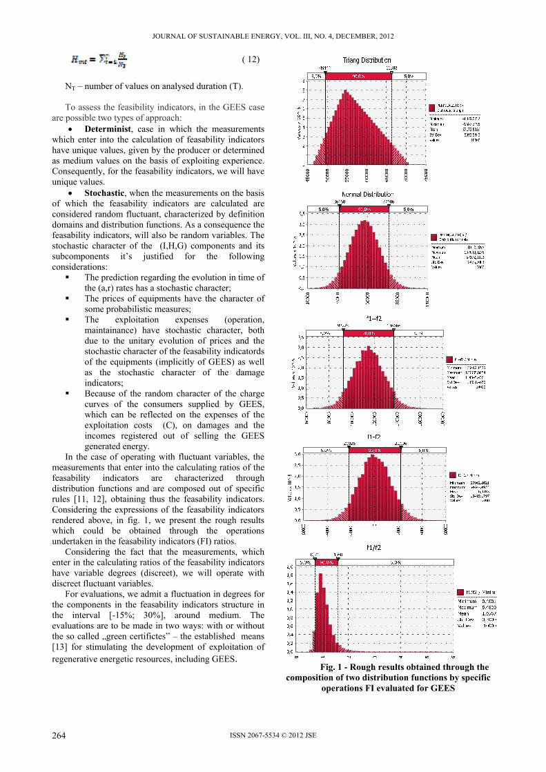
JOURNAL OF SUSTAINABLE ENERGY, VOL. III, NO. 4, DECEMBER, 2012
ISSN 2067-5534 © 2012 JSE
( 12)
NT – number of values on analysed duration (T). To assess the feasibility indicators, in the GEES case
are possible two types of approach: Determinist, case in which the measurements
which enter into the calculation of feasability indicators have unique values, given by the producer or determined as medium values on the basis of exploiting experience. Consequently, for the feasability indicators, we will have unique values.
Stochastic, when the measurements on the basis of which the feasability indicators are calculated are considered random fluctuant, characterized by definition domains and distribution functions. As a consequence the feasability indicators, will also be random variables. The stochastic character of the (I,H,G) components and its subcomponents it’s justified for the following considerations: The prediction regarding the evolution in time of
the (a,r) rates has a stochastic character; The prices of equipments have the character of
some probabilistic measures; The exploitation expenses (operation,
maintainance) have stochastic character, both due to the unitary evolution of prices and the stochastic character of the feasability indicatords of the equipments (implicitly of GEES) as well as the stochastic character of the damage indicators;
Because of the random character of the charge curves of the consumers supplied by GEES, which can be reflected on the expenses of the exploitation costs (C), on damages and the incomes registered out of selling the GEES generated energy.
In the case of operating with fluctuant variables, the measurements that enter into the calculating ratios of the feasability indicators are characterized through distribution functions and are composed out of specific rules [11, 12], obtaining thus the feasability indicators. Considering the expressions of the feasability indicators rendered above, in fig. 1, we present the rough results which could be obtained through the operations undertaken in the feasability indicators (FI) ratios.
Considering the fact that the measurements, which enter in the calculating ratios of the feasability indicators have variable degrees (discreet), we will operate with discreet fluctuant variables.
For evaluations, we admit a fluctuation in degrees for the components in the feasability indicators structure in the interval [-15%; 30%], around medium. The evaluations are to be made in two ways: with or without the so called „green certifictes” – the established means [13] for stimulating the development of exploitation of regenerative energetic resources, including GEES.
Fig. 1 - Rough results obtained through the
composition of two distribution functions by specific operations FI evaluated for GEES
264

JOURNAL OF SUSTAINABLE ENERGY, VOL. III, NO. 4, DECEMBER, 2012
ISSN 2067-5534 © 2012 JSE
3. CASE STUDIES
In the present paper, we will exemplify the methodology for making a feasability study with reference to electro-geothermal plant with binary cycle (EGPB), represented graphically in fig. 2. In the analysis only the main elements of EGPB are considered, while the price for drilling lead is ignored, considering the fact that the plant uses an already existing drill. For the stochastic analysis of feasability we use the @Risk programme [14].
Forward we will present , two examples of the EGPB feasability analysis, one without the value of green certificates, and the second one considering the grant received under the form of green certificates, taking into consideration the triangle distribution components of the investment expenses.
In table 1 there are presented the actual medium prices (for start) of each equipment at once, on the basis of which the total cost of EGPB was calculated, and in tabel 2 an estimation of the prices for the 5 components, with the inferior limit lower costs with 15%, and superior limit, that is „maxim costs” with an exceeding of medium cost with 30 %, is made for each component.
The medium costs for each equipment are taken from [3, 4, 15] and in [9] we find the medium price on kW installed for the ORC plants which has as a primary source the geothermal energy . This price is of 2259 USD/kW.
Tabel 1 - Average costs equipment for CEGB
No Components of
power plant
Cost [EUR]
Size [kW]
or [m2]
Cost/equipment [EUR]
1 Vaporizer 330 309 101970
2 Preheater 330 165 54450
3 Turbine-Generator
500 500 250000
4 Condenser 330 790 260700
5 Pump 500 5,5 2750
6. Total 669870
Tabel 2. Cost values for triangle distribution
No Components Minimum
[EUR]
Most likely
[EUR]
Maximum
[EUR]
1. Vaporizer 86674,5 101970 132561
2. Preheater 46282,5 54450 70785
3. Turbine-Generator 212500 250000 325000
4. Condenser 221595 260700 338910
5. Pump 2337,5 2750 3575
After introducing the value of equipment costs in the working sheet, we generted for each the triangle
distribution. Also, there is calculated the risk in such a manner that the value of the project should exceed with 10%, 50% şi 90% , the result of the distributions. In fig. 3 there is presented an image of the screen during evaluation, during executing the programmed number of iterations, and in fig.4 there is presented the triangle distribution for the total cost.
Fig. 3 - The screen image with the evaluation process
Fig. 4 - The triangle distribution for the total cost
estimation
The probability that the value of the project would exceed the estimated budget is of 49%, thus justifying the determination of the feasability indicators. The estimated cost for attendance (maintainance) and for the employees wages, for an year is of 50.000 EUR, and the medium production of the plant is 403 kW, thus in a whole year the plant produces supplies of 3,53 GWh. The price received for the supplied energy is of 45 Euro/MWh according to [13]Eroare! Fără sursă de referinţă..
The above undertaken simultation includes only the costs for the main components of the plant, which is not enough, because the cost of the entire plant is different , according to [9], to the components price one shoul add (auxilliary components, execution manufacturing, s.o.) 300 $/kW for determining the cost of the whole plant, and the rate Euro/Dollar is: 1 EUR =1,22 USD. Considering this aspect to the total cost of the components, one shoul add (300 $/kW=246 EUR/kW).
a.) Results without „green certificates” (scenary1) The price encashed for the sold energy in a year is:
Cw = 3530 ·45 =158.850 EUR In fig. 5 – fig. 7. are represented the distributions of the feasibility indicators : the necessary time for recovering the investment, the actual net earning and the profit index.
Triang Distribution
265

JOURNAL OF SUSTAINABLE ENERGY, VOL. III, NO. 4, DECEMBER, 2012
ISSN 2067-5534 © 2012 JSE
Fig. 5 - The distribution of „DR” indicator
Fig.6 - The distribution of „VNA” indicator
Fig. 7 - The distribution of „IP”indicator b.) Results with „green certificates” (scenary 2)
According to Law no. 220/2008 [13] Eroare! Fără sursă de referinţă. for each MW of raw power supplied in the electric network one can get 2 green certificates , the price for one green certificate being of 53 EUR/MWh. Taking into consideration the efficiency of the generator (96%), the raw power of the plant is of 420 kW. The total price of the green certificates for an entire year is : 420·2·53·8,760 = 389.995 EUR/year.
In the hypotesis of possible incomes out of green certificates the feasiblity indicators are changed as in fig.8 – fig. 10.
Fig. 8 - The distribution of „DR” indicator with green certificates
Fig. 9 - The distribution of „VNA” indicator with green certificates
Fig. 10 - The distribution of „IP”indicator with green certificates
The results of the evaluation made in the hypotesis of
normal distribution of the random variable subcomponents „I” and other details are presented in [16].
266

JOURNAL OF SUSTAINABLE ENERGY, VOL. III, NO. 4, DECEMBER, 2012
ISSN 2067-5534 © 2012 JSE
4. CONCLUSIONS For the feasibility analysis of EGPB one can use
the following feasibility indicators: the time for recovering the investment, the actual net earning and the profit index
In case of EGPB for calculating the feasibility indicators one should know the following values: the investment (I), the economic effect(Ht), the economic effort (Gt), the time for analysis (T).
Taking into consideration the stochastic charcater of the values which enter into the ratio which calculates the feasibility indicators, it is recommended in order to increase the accuracy of EGPB feasibility analysis, to operate with random variables, characterized through distribution functions and definition domains.
Following the operation of triangle and normal distributions for EGPB feasibility analysis, one can notice: In case of scenary 2, due to the grants received from
the state (green certificates) the time for recovering the investment is considerably reduced with values up to 6 years, in comparison with scenary 1 ;
The values of feasibility indicators for the two tested distributions (triangle and normal) are closed;
In case of scenary 2, the time for recovering the investment is under 2 years, which means that the project is feasible;
The equipments which influence considerably the costs of the plant are: the condenser and the engine-generator assembly.
REFERENCES
[1] ** Directiva 2009/28/CE a Parlamentului European �i a Consiliului din 23 aprilie 2009 privind promovarea utilizării energiei din surse regenerabile, de modificare �i ulterior de abrogare a directivelor 2001/77/CE �i 2003/30/CE. [2] Cleveland C.J., Encyclopedia of Energy, Vol 1÷6 Elsevier Academic Press, 2004. [3] Schuster A, Karellas S, Kakaras E, Spliethoff H. - Energetic And Economic Investigation Of Organic Rankine Cycle Applications, Applied Thermal Engineering, 2008. [4] Tchanche B., Quoilin S., Declaye S., Papadakis G., Lemort V. - Economic Optimization Of Small Scaleorganic Rankine Cycles, 2010, pdf. [5] Ruggero B. - Geothermal Power Generation in the World 2005–2010 Update Report, Proceedings World Geothermal Congress 2010, WGC2010; [6] Rosca M. - Geotermalism şi centrale geotermale, Editura Universităţii din Oradea, 1999 [7] Felea I., ManolescuM.J. - Applying the Reliability Theory to the Investigation and Optimization of the Complex Geothermal Uses, Proceedings of the World Geothermal Congress, vol 4/1995. [8] Carabulea A., Felea I. - Managementul Riscului Energetic, Partea II, Universitatea Politehnica Bucuresti, Facultatea de Energetica, Catedra Management Industrial, 2000. [9] Baz González E. - Feasibility Study of Geothermal Utilization of Remoteness Areas, Design an Optimization of a Small Standard Power Plant”, University of Iceland & University of Akureyri, February 2011 [10] Felea I. - Ingineria Fiabilită�ii în Electroenergetică, Editura Didactică �i pedagogică, Bucure�ti, 1996. [11] Mihoc Gh., et.a., - Bazele Matematice ale Teoriei Fiabilităţii, Ed. Dacia, Cluj-Napoca, 1976. [12] Panaite V., Munteanu R., - Control Statistic şi Fiabilitate, EDP, Bucureşti, 1982. [13] ***www.anre.ro [14] Sun Caixia, - Feasibility Study of Geothermal Utilization of Yangbajain Field in Tibet Autonomous Region, P.R.China, Msc Thesis, UNU-GTP, 2008. [15] Panea C. - Studii Şi Cercetări Privind Performanţele Energetice Şi De Disponibilitate Ale Sistemelor De Valorificare A Resurselor Geotermale Cu Entalpie Scăzută, Teza de doctorat, Universitatea din Oradea, 2012.
267