T U MI N S T I T U T F U R I N F O R M A T I K

Modular and Visual Specification of HybridSystems

– An Introduction to HyCharts –

Radu Grosu and Thomas Stauner

ABCDEFGHIJKLMNOTUM-I9801

Dezember 98

T E C H N I S C H E U N I V E R S I TA T M U N C H E N

TUM-INFO-12-I9801-80/1.-FIAlle Rechte vorbehaltenNachdruck auch auszugsweise verboten

c 1998

Druck: Institut f ur Informatik derTechnischen Universit at M unchen

Modular and Visual Speci�cation of HybridSystems{ An Introduction to HyCharts {Radu Grosu and Thomas Stauner1Institut f�ur Informatik, Technische Universit�at M�unchenD-80290 M�unchen, Germanyhttp://www4.informatik.tu-muenchen.de/Email: fgrosu,staunerg@informatik.tu-muenchen.de

1The second author was supported with funds of the Deutsche Forschungsgemein-schaft under reference number Br 887/9-1 within the priority program Design anddesign methodology of embedded systems.

AbstractVisual description techniques are particularly important for the design of hybridsystems because speci�cations of such systems usually have to be discussed be-tween engineers from a number of di�erent disciplines. Modularity is vital forhybrid systems not only because it allows to handle large systems, but also be-cause hybrid systems are naturally decomposed into the system itself and itsenvironment.Based on two di�erent interpretations for hierarchic graphs and on a clearhybrid computation model, we develop HyCharts. HyCharts consist of two mod-ular visual formalisms, one for the speci�cation of the architecture and one forthe speci�cation of the behavior of hybrid systems. The operators on hierarchicgraphs enable us to give a surprisingly simple denotational semantics for manyconcepts known from statechart-like formalisms. Due to a very general composi-tion operator, HyCharts can easily be composed with description techniques fromother engineering disciplines. Such heterogeneous system speci�cations seem tobe particularly appropriate for hybrid systems because of their interdisciplinarycharacter.

Contents1 Introduction 11.1 An Example . . . . . . . . . . . . . . . . . . . . . . . . . . . . . . 11.2 Related Work . . . . . . . . . . . . . . . . . . . . . . . . . . . . . 31.3 Overview . . . . . . . . . . . . . . . . . . . . . . . . . . . . . . . . 52 Hierarchic Graphs 62.1 Syntax . . . . . . . . . . . . . . . . . . . . . . . . . . . . . . . . . 62.1.1 Operators on Nodes . . . . . . . . . . . . . . . . . . . . . . 62.1.2 Connectors. . . . . . . . . . . . . . . . . . . . . . . . . . . 82.1.3 An Example . . . . . . . . . . . . . . . . . . . . . . . . . . 82.2 The Additive Model . . . . . . . . . . . . . . . . . . . . . . . . . 92.2.1 Arrows . . . . . . . . . . . . . . . . . . . . . . . . . . . . . 92.2.2 Nodes and Operators . . . . . . . . . . . . . . . . . . . . . 102.3 The Multiplicative Model . . . . . . . . . . . . . . . . . . . . . . 122.3.1 Arrows . . . . . . . . . . . . . . . . . . . . . . . . . . . . . 122.3.2 Nodes and Operators . . . . . . . . . . . . . . . . . . . . . 133 The Hybrid Computation Model 163.1 General Idea . . . . . . . . . . . . . . . . . . . . . . . . . . . . . . 163.2 The Combinational Part . . . . . . . . . . . . . . . . . . . . . . . 183.3 The Analog Part . . . . . . . . . . . . . . . . . . . . . . . . . . . 193.4 The Component . . . . . . . . . . . . . . . . . . . . . . . . . . . . 203.5 A Note on Semantics . . . . . . . . . . . . . . . . . . . . . . . . . 224 System Architecture Speci�cation - HyACharts 235 Component Speci�cation - HySCharts 255.1 The Combinational Part . . . . . . . . . . . . . . . . . . . . . . . 255.2 The Analog Part . . . . . . . . . . . . . . . . . . . . . . . . . . . 313

46 Relation to Other Formalisms 346.1 Heterogeneous Component Speci�cation . . . . . . . . . . . . . . 346.2 Timed Automata . . . . . . . . . . . . . . . . . . . . . . . . . . . 346.3 A Typical Hybrid Component . . . . . . . . . . . . . . . . . . . . 357 Conclusion 36

Chapter 1IntroductionHybrid systems have been a very active area of research over the past few yearsand a number of speci�cation techniques have been developed for such systems.While they are all well suited for closed systems, the search for hybrid descriptiontechniques for open systems is relatively new.For open systems { as well as for any large system { modularity is essential. Itis not only a means for decomposing a speci�cation into manageable small parts,but also a prerequisite for reasoning about the parts individually, without havingto consider the interior of other parts. Thus, it greatly facilitates the designprocess and can help to push the limits of veri�cation tools, like model-checkers,further.With a collection of operators on hierarchic graphs as our tool-set, we followthe ideas in [GSB98] and de�ne a simple and powerful computation model for hy-brid systems. Based on this model we introduce HyCharts, which consist of twodi�erent interpretations of hierarchic graphs. Under one interpretation the graphsare called HySCharts under the other one they are called HyACharts. HySChartsare a visual representation of hybrid, hierarchic state transition diagrams. Hy-ACharts are a visual representation of hybrid data- ow graphs (or architecturegraphs) and allow the designer to compose hybrid components in a modular way.The behavior of these components can be described by using HySCharts or byany technique from system theory that can be given a semantics in terms of denseinput/output relations. This includes di�erential equations. Dense input/outputrelations are a relational extension of hybrid Focus [MS97, Bro97].1.1 An ExampleThe following example illustrates the kinds of systems we target at. It will beused throughout the paper to demonstrate the use of HyCharts.Example 1 (An electronic height control system, EHC) The purpose ofthis system, which was originally proposed by BMW, is to control the chassis level1

2of an automobile by a pneumatic suspension. The abstract model of this system,which considers only one wheel, was �rst presented in [SMF97]. It basically worksas follows:Whenever the chassis level is below a certain lower bound, a compressor isused to increase it. If the level is too high, air is blown o� by opening an escapevalve. The chassis level sHeight is measured by sensors and �ltered to eliminatenoise. The �ltered value fHeight is read periodically by the controller 1 whichoperates the compressor and the escape valve and resets the �lter when necessary.A further sensor, inBend , tells the controller whether the car is going through acurve.The diagram in Figure 1.1, left, depicts the architecture of the EHC and itsinterconnection to the environment. The environment, shaded in grey in the�gure, will not be regarded further in this paper. Instead we concentrate onthe open system consisting of the �lter, the controller and a delay element thatensures that the feed-back is well-de�ned. The escape valve and the compressorare modeled within the controller.[

[

[

[

[

Df

)

[)

[)EHC

FilterfHeight

resetdReset

Control

ENVaHeight

inBend

sHeight

aHeight

fHeight

dReset

sHeight

time

[)

t"t t’Figure 1.1: The EHC: Architecture and a typical evolution.Diagrams like the one in Figure 1.1, left, are called HyACharts. Each com-ponent of such a chart can be de�ned again by a HyAChart or by a HySChartor some other compatible formalism. The components only interact via clearlyde�ned interfaces, namely channels, which results in a modular speci�cation tech-nique.The behavior of a component is characterized, as intuitively shown in Figure1.1, right, by periods where the values on the channels change smoothly and bytime instances at which there are discontinuities. In our approach the smoothperiods result from the analog parts of the components. The discontinuities arecaused by their combinational (or discrete) parts.1Note that periodical sampling can be avoided in a hybrid model. However, it was used inthe BMW implementation and it allows us to expose various features of our formalism, likeentry/exit actions and timeouts.

3We specify the behavior of both the combinational and the analog part of acomponent within a single HySChart, i.e., by a hybrid, hierarchic state transitiondiagram, with nodes marked by activities and transitions marked by actions. Thetransitions de�ne the discontinuities, i.e., the instantaneous actions performed bythe combinational part. The activities de�ne the smooth periods, i.e., the timeconsuming behavior of the analog part while the combinational part is idle. As

i2di2u

reset

n2b b2n

Control

b2n

reset

n2b

outTol

u2d

d2ud2i

reset

d2d

outTolu2i

i2d

i2ui2i

u2u

w_inct_o

t_ot_o

inTol

up down

a_const

a_inc a_deca_const

outBend

outBend

inBend

Figure 1.2: The EHC's Control component.an example, Figure 1.2 shows the HySChart for the EHC's Control component.It consists of three hierarchic levels. Figure 1.2, left, depicts the highest level.Figure 1.2, top right, re�nes the state outBend and Figure 1.2, bottom right,further re�nes the state outTol . The states, transitions and activities (written initalics in the �gure) are explained in Chapter 5. �1.2 Related WorkThe basic motivation for this work were experiences we obtained when modelingthe EHC case study outlined above with hybrid automata [SMF97]. A basicresult of the case study was that the lack of modularity of hybrid automatacomplicates speci�cation and analysis. Furthermore, the lack of hierarchic statesturned out to be inconvenient for speci�cation. In this work, we develop a formal,modular description technique for hybrid systems that is associated with a visualformalism and incorporates advanced state machine features such as hierarchicstates and preemption. In contrast to hybrid automata [ACH+95], HyCharts arefully modular and suitable for open systems.The rather new hybrid modules from Alur and Henzinger [AH97] are modular,but their utility su�ers from the fact that it is not obvious how to model feedback

4loops. For theoretical reasons, loops pose a problem in our approach, too. Wesolve it by explicitly allowing feedback loops, as long as they introduce a delay.Demanding a delay is not unrealistic, as signals cannot be transmitted at in�nitespeed.Another modular model, hybrid I/O automata, is presented in [LSVW96].While this model is promising from the theoretical point of view, we think ithas some de�cits in practice. In particular, there is no graphical representationfor hybrid I/O automata yet, there is no hierarchy concept for them and �nally,there is no visual formalism for the speci�cation of the architecture of a composedsystem. The same applies for the hybrid modules mentioned above. From thesystems engineering point of view our approach is therefore more convenient.A �rst approach towards a hybrid version of statecharts can be found in[KP92]. The operational semantics given there, however, does not allow inter-level transitions and hierarchic speci�cation of continuous activities. Therefore,this approach does not fully support hierarchy, unlike HyCharts, which permitboth.Except for HyCharts all the models mentioned above are based on some kindof trace semantics in which continuous trajectories are pasted together at dis-crete time instances. At these instances, the preceding trajectory, the succeedingtrajectory and possibly some intermediate discrete actions determine the valuesfor the variables in the model. As the end point of the preceding trajectory,the values determined by intermediate discrete actions and the start point of thesucceeding trajectory need not be equal we get situations in which one variable isassigned a sequence of values at the same physical time instant. This means thatsuch a trace is not isomorphic to a function of time. In our opinion this makesit di�cult to combine the above models with models for continuous systems, asthey evolved in the engineering disciplines, di�cult. A decision must be madethat determines which value of the variable is to be \exported", i.e. visible tothe outside world at a physical time instant. For hybrid automata, for instance,intermediate values in a sequence of discrete actions can cause further actions inparallel components. Thus, such a decision is hardly possible. For HyCharts weuse a simpler form of traces. Here, any variable has exactly one value at eachtime instant, the variable evaluation is a function of time.Commercial products for the design of embedded systems, like StateFlow[TMI98], take a di�erent approach to specifying hybrid systems. In this approachthe system needs to be partitioned into purely discrete and purely continuouscomponents before speci�cation can begin. While this method may be appropri-ate for many systems we think it enforces a too early partitioning into hardwareand software components and is highly inconvenient for specifying componentsthat are hybrid themselves, like some environment models, which, for example,contain phase transitions. A formal model that uses a speci�cation approach sim-ilar to StateFlow can be found in [EH96]. Interestingly there are some parallelsbetween our hybrid machine model (Chapter 3) and the model presented there.

5To end this journey through the literature we want to mention that HyChartslook largely similar to the description techniques used in the software engineeringmethod for real-time object-oriented systems ROOM [SGW94] and may thereforebe seen as a hybrid extension of them.1.3 OverviewThe rest of the paper is organized as follows. In Chapter 2 we present two abstractinterpretations of hierarchic graphs. These interpretations provide the infrastruc-ture for de�ning a surprisingly simple denotational semantics for the key conceptsof statecharts [Har87] o�ered in HyCharts, like hierarchy and preemption. Theyalso are the foundation for the denotational semantics of our hybrid computa-tion model, which is introduced in Chapter 3. Following the ideas developed inthis model, HyCharts are de�ned in Chapters 4 and 5 as a multiplicative andan additive interpretation of hierarchic graphs, respectively. Both diagram kindsare introduced in an intuitive way by using the example above. In Chapter 6 webrie y discuss how other techniques for component speci�cation can be integratedinto our approach and relate HySCharts to timed automata. Furthermore, wediscuss the HyChart speci�cation of the �lter component from our example sys-tem and its importance for hybrid modeling. Finally, in Chapter 7 we summarizeour results.

Chapter 2Hierarchic GraphsThis chapter �rst introduces an algebra of hierarchic graphs (Section 2.1). Thentwo models, an additive and a multiplicative model, for this algebra are given.The additive model interprets the operators in a way that results in control- owgraphs (Section 2.2), the multiplicative model interprets them in a way that yieldsdata- ow graphs (Section 2.3).2.1 SyntaxA hierarchic graph consists of a set of nodes connected by a set of arcs. Foreach node, the incoming and the outgoing arcs de�ne the node's interface, i.e. itstype. Let A and B be the input and the output interfaces of a node n. Then thecorresponding textual notation for n is n : A! B (Fig. 2.1). Interpreting A andB as sets (or types) n may be regarded as a mapping from elements of A intoelements of B.A

nBFigure 2.1: A node n : A! B.2.1.1 Operators on NodesIn order to obtain graphs, we put nodes next to one another and connect themby using the following operators on relations: sequential composition, visual at-tachment and feedback. Their respective visual representation is given in Figure2.2.Sequential composition. One basic way to connect two nodes is by sequentialcomposition, i.e., as shown in Figure 2.2, left, by connecting the output of one6

7A B C

n2

B2

n2

Visual attachment FeedbackSequential composition

n1

A2A1

1B

n1

B

A

C

n

Figure 2.2: The composition operators.node to the input of the other node, if they have the same type. Textually wedenote this operator by the semicolon ;. Given n1 : A ! B and n2 : B ! C wede�ne n1;n2 to be of type n1;n2 : A! C.Regarding the nodes as computation units, Figure 2.2, left, says that theoutput produced by n1 is directed to the input of n2. The connection between n1and n2 as well as the units n1 and n2 themselves, are internal to n1;n2. In otherwords, n1;n2 does not only de�ne a connection relation but also a containmentrelation.Visual attachment. By visual attachment we mean that nodes and corre-sponding arrows are put one near the other, as shown in Figure 2.2, middle. Toobtain a textual representation for visual attachment, we need an attachmentoperator both on arrows and on nodes. We denote this operator by ?. Giventwo arrows A and B their visual attachment is expressed by A ? B. Given twonodes n1 : A1 ! B1 and n2 : A2 ! B2 their visual attachment is expressed asn1?n2 : A1?A2 ! B1?B2. Visual attachment also de�nes a containment relation.We say that n1 and n2 are contained in n1 ? n2.In order to deal with hiding it is convenient to explicitly introduce an arrowE denoting the absence of any information. This arrow is neutral for attachment,i.e. A ? E = E ? A = A, because visually attaching nothing does not change theoriginal information.Feedback. Sequential composition allows us to connect the nodes of a graphin a causal way. However, using only sequential composition to connect nodesis not expressive enough because it cannot deal with loops or with bidirectionalcommunication. We therefore introduce a feedback operator, as shown in Figure2.2, right. It allows us to connect the rightmost output of a node to the rightmostinput of the same node, if they have the same type. Given n : A?C ! B ?C wede�ne n "CA;B: A! B. Similar to sequential composition and visual attachment,feedback also introduces a containment relationship. We say that n and thefeedback arrow are contained in n "CA;B.Nodes and arrows that are not built up from other nodes or arrows using theabove operators are called primitive.

82.1.2 Connectors.Beside operators on nodes, we also need some operators on arcs (or prede�nednodes), which we call connectors. We consider the following connectors: identity,identi�cation, rami�cation and transposition. Their visual representation is givenin Figure 2.3.A

A A A

A

identity identification ramification transposition

A

A

A A B

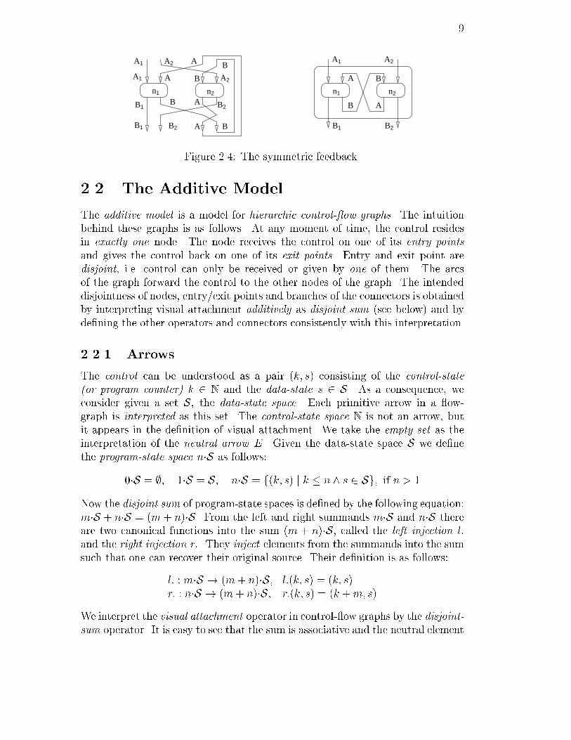
B AFigure 2.3: The connectors.Identity. The identity connector IA simply copies its input to the output. Ithas type A! A.Identi�cation. The identi�cation connector _kA joins k inputs together. Itstype is Ak ! A, where Ak = A ? : : : ? A stands for the k-fold attachment of A.For k = 0 we de�ne A0 = E, i.e. the neutral arrow. In Figure 2.3 the binary caseis depicted.Rami�cation. The rami�cation connector ^Ak copies the input information onk outputs. Hence ^Ak has type A! Ak. Figure 2.3 shows the binary case.Transposition. Finally the transposition connector AXB exchanges the inputs.Its type is A ? B ! B ? A.To be a precise formalization of our intuitive understanding of graphs, theabove abstract operators and connectors have to satisfy a set of laws, which in-tuitively express our visual understanding of graphs. These laws correspond tostrict, symmetric, monoidal categories with feedback and bimonoid objects, seee.g. [Ste94]. [GSB98] shows that the additive and the multiplicative interpre-tations of the operators and connectors are particularly relevant for computerscience.2.1.3 An ExampleAs an example for a hierarchic graph and its corresponding textual respresenta-tion we consider the graph in Figure 2.4, left. Using the above basic operatorsand connectors it de�nes a derived composition operator, the symmetric feed-back. If n1 : A1 ? A ! B1 ? B and n2 : B ? A2 ! A ? B2 then n1�? n2 has typeA1?A2 ! B1?B2. Its simpli�ed visual representation is given in Figure 2.4, right.The textual respresentation corresponds one to one to the visual representationin Figure 2.4, left:n1�? n2=(((IA1 ? A2xA?B);(n1 ? n2);(IB1 ? B?AxB2);(IB1?B2 ? BxA))"B? )"A?

9B A

B

n1 n2

B1

B1

A1

A1 2 A

A B2

2

A2

BA

A

B

B

A

A B

n1 n2

A1 A2

B2B1

BFigure 2.4: The symmetric feedback.2.2 The Additive ModelThe additive model is a model for hierarchic control- ow graphs. The intuitionbehind these graphs is as follows. At any moment of time, the control residesin exactly one node. The node receives the control on one of its entry pointsand gives the control back on one of its exit points. Entry and exit point aredisjoint, i.e. control can only be received or given by one of them. The arcsof the graph forward the control to the other nodes of the graph. The intendeddisjointness of nodes, entry/exit points and branches of the connectors is obtainedby interpreting visual attachment additively as disjoint sum (see below) and byde�ning the other operators and connectors consistently with this interpretation.2.2.1 ArrowsThe control can be understood as a pair (k; s) consisting of the control-state(or program counter) k 2 N and the data-state s 2 S. As a consequence, weconsider given a set S, the data-state space. Each primitive arrow in a ow-graph is interpreted as this set. The control-state space N is not an arrow, butit appears in the de�nition of visual attachment. We take the empty set as theinterpretation of the neutral arrow E. Given the data-state space S we de�nethe program-state space n�S as follows:0�S = ;; 1�S = S; n�S = f(k; s) j k � n ^ s 2 Sg; if n > 1Now the disjoint sum of program-state spaces is de�ned by the following equation:m�S + n�S = (m + n)�S. From the left and right summands m�S and n�S thereare two canonical functions into the sum (m + n)�S, called the left injection l:and the right injection r:. They inject elements from the summands into the sumsuch that one can recover their original source. Their de�nition is as follows:l: : m�S ! (m+ n)�S; l:(k; s) = (k; s)r: : n�S ! (m + n)�S; r:(k; s) = (k +m; s)We interpret the visual attachment operator in control- ow graphs by the disjoint-sum operator. It is easy to see that the sum is associative and the neutral element

10is 0�S. In the following we will often merely refer to the program-state as thestate.2.2.2 Nodes and OperatorsA node n : A ! B of a control- ow graph is interpreted as a relation n �(I � k�S) � l�S between the current input, the current control and the nextcontrol. Upon receiving the current control state, it determines the next controlstate, depending on the current input. In addition, we consider an externalinput here, because the sequential machines de�ned by the relations are allowedto communicate with their environment. They may receive inputs and produceoutputs. The output space simply is a projection of the data-state space. Wewrite I to denote the input space. The de�nition of the operators below ensuresthat all nodes receive the same input. Therefore, by convention no arrow isdrawn to denote the external input I to a node. Note that in order to simplifynotation, we use the same name for the node, which is a syntactic entity, andits associated relation, which is a semantic entity. In the following we denotearbitrary program-state spaces x � S and xi � S over data-state space S by X andXi for x 2 fa; b; cg .The Node OperatorsSequential composition. The sequential composition of two nodesn1 � (I � A) � B; n2 � (I �B) � Cyields, a new node n1 ; n2, which is de�ned as expected:n1 ; n2 � (I � A) � Cn1 ; n2 = f(x; a; c) j 9b 2 B: (x; a; b) 2 n1 ^ (x; b; c) 2 n2gAdditive composition. The additive composition of two nodesn1 � (I � A1) � B1; n2 � (I � A2) � B2yields, as in statecharts, a new node n1 + n2, such that control resides either inn1 or in n2. Note that the interface of the sum re ects this fact.n1 + n2 � (I � (A1 + A2)) � (B1 +B2)n1 + n2 = f(x; l:a; l:b) j (x; a; b) 2 n1g [ f(x; r:a; r:b) j (x; a; b) 2 n2gThe visual notation of n1 + n2 is given in Figure 2.5, left. The meaning of(n1 + n2)(x; l:a) is intuitively shown in Figure 2.5, right. Receiving the tuple(x; l:a), the sum uses the control information l to \demultiplex" the input andselect the corresponding relation n1; this relation is then applied to (x; a) to

11n2

l.b

l.a

n121n

l.a r.a

r.b

n

l.b

21

1 2Figure 2.5: The additive interpretation.obtain the next state b; �nally, the output of the relation is \multiplexed" to l:b.Additive feedback. The additive feedback is more tricky and it allows theconstruction of loops. As in programming, feedback has to be used with care inorder to ensure termination. Given a relationn � (I � (A + C)) � (B + C)we de�ne the relation n"C+ as follows: The control is received on A and it is eithergiven directly on B or after an arbitrary number of times in which it loops alongC. Formally: n"C+ � (I � A) � Bn"C+ = nl;l [ nl;r ; n�r;r ; nr;lwhere n� is the arbitrary but �nite iteration of n and ni;j is de�ned for i; j 2 fl; rgas below: ni;j = f(x; s; s0) j (x; i:s; j:s0) 2 ngIn this de�nition l and r are the injections corresponding to A and C for theinput and to B and C for the output.The ConnectorsIdentity. The identity IA is de�ned as expected:IA � (I � A)� A; IA = f(x; a; a) j a 2 A ^ x 2 IgAdditive identi�cation. The additive identi�cation k>�A forgets the entrypoint on which it gets the control:k>�A � (I � k A)� A;k>�A = f(x; i:a; a) j 0 < i � k ^ a 2 A ^ x 2 Igwhere k A = k (a � S) = (k � a) � S.

12Additive rami�cation. The additive rami�cation A�<k gives the control onany of its exit points:A�<k � (I � A)� k A;A�<k = f(x; a; i:a) j 0 < i � k ^ a 2 A ^ x 2 IgAdditive transposition. The additive transposition BA=n commutes the entrypoint information:BA=n � (I � (A+B))� B + A;BA=n = f(x; l:a; r:a) j a 2 A ^ x 2 Ig [ f(x; r:b; l:b) j b 2 B ^ x 2 IgThis means that control is passed on along the right exit point if it was receivedon the left entry point and vice versa.2.3 The Multiplicative ModelThe multiplicative model is a model for hierarchic data- ow graphs. The intuitionbehind these graphs is as follows. At any moment of time, all nodes of the graphare active and computing the output data based on the input data. A nodereceives the input data along a tuple of input channels and sends the computeddata along a tuple of output channels. The arcs of the graph, i.e., the channels,forward the data to the other nodes in the graph. The intended parallelismof nodes, input/output channels and branches of the connectors is obtained byinterpreting the visual attachment ? multiplicatively by the product � and byde�ning the other operators and connectors consistently with this interpretation.2.3.1 ArrowsWe assume given a set of channel types D = fDi j i 2 Ng, each de�ning the setof messages which is allowed to ow along a channel. The input and the outputinterface type of a component, respectively, is then a product A = A1�: : :�Anof channel types Ai 2 D, de�ned as follows:A = f()g if n = 0; A = A1 if n = 1;A = f(x1; : : : ; xn) j x1 2 A1 ^ : : : ^ xn 2 Ang if n > 1Given arbitrary interface types A = A1� : : :�Am and B = B1� : : :�Bn. Weextend the above product de�nition as follows:A�f()g = f()g�A = AA�B = A1 � : : :� Am � B1 : : :� Bn

13Hence, the empty interface f()g is the neutral arrow E. The left and rightprojections p: and q: are given below:p: : A1�: : :�Am�B1: : :�Bn ! A1�: : :�Am;p:(a1; : : :; am; b1; : : :; bn) = (a1; : : :; am)q: : A1�: : :�Am�B1: : :�Bn ! B1�: : :�Bn;q:(a1; : : :; am; b1; : : :; bn) = (b1; : : :; bn)The projections uniquely de�ne a pairing function (:; :) such that for any C,f = (f1; : : :; fm) 2 C ! A and g = (g1; : : :; gn) 2 C ! B it holds that: (f; g) =(f1; : : :; fm; g1; : : :; gn). By de�nition, the product is associative and has as neutralelement E. The unique existence of projections is characteristic for data- owgraphs.In data- ow graphs the main concern is the data ow . To de�ne and analyzethis ow, we need to observe the information exchanged along each channel overtime. In a hybrid system this ow may be continuous (think of analog devices),so we assume that time increases continuously, i.e. it is dense, and take the non-negative real numbers R+ as abstract time axis. In this case, the data exchangedalong a channel with type A over time de�nes a mapping a 2 AR+. Motivatedby our hybrid computation model (Chapter 3) we impose some restrictions onthis mapping in the next chapter. We call such a restricted mapping a densecommunication history and its corresponding type a dense communication historytype. The latter ones are used to interpret the primitive arrows of data- owgraphs.A reasonable assumption which leads to a model with very nice properties, isthat data- ows are time synchronous, i.e., that time ows in the same way for eachchannel and each component. In this case, the history (and its associated pre�x-ordering) of a component's interface (A1�: : :�Am)R+ is equal to the productAR+1 �: : :�AR+m of the histories of its channels.2.3.2 Nodes and OperatorsThe behavior of a component can be completely described by an input/outputrelation, i.e., by a relation between the histories of its input channels and thehistories of its output channels. The relation must be total in the input histories.We assume that the relations are de�ned such that the data occurring in thehistories of the output channels at time t only depends on the input historyreceived up to (and including) t. Formally, for all a1; a2 and t:a1#[0;t] = a2#[0;t] ) n(a1)#[0;t] = n(a2)#[0;t]where by a#� we denote the restriction of a to the time interval �. Clearly, eachrealizable component behaves in this way. We call these relations time guarded.

14They interpret the nodes of the data- ow graphs. To simplify notation, we usethe same name (or symbol) for a node (or operator) and its associated relation (orrelational operator). Note, however, that the names and symbols are syntacticentities whereas the relations and relational operators are semantic entities.The Node OperatorsSequential composition. The interpretation of sequential composition is theusual sequential composition of relations. It allows passing of the data from onecomponent to another component in a linear way. Given two relations:n1 � AR+ � BR+; n2 � BR+ � CR+we de�ne their sequential composition n1 ; n2 as follows:n1 ; n2 � AR+ � CR+n1 ; n2 = f(a; c) j 9b 2 BR+: (a; b) 2 n1 ^ (b; c) 2 n2gParallel composition. As in statecharts, the parallel composition of two com-ponents yields a new component such that both constituents are active simul-taneously, i.e. each constituent has its own control, described for example by acontrol- ow graph. The interface of the product has to re ect this fact. Giventwo relations n1 � A1R+ � B1R+; n2 � A2R+ � B2R+we de�ne their product n1 � n2 as follows:n1 � n2 � (A1R+ � A2R+) � (B1R+ �B2R+)n1 � n2 = f((a1; a2); (b1; b2)) j (a1; b1) 2 n1 ^ (a2; b2) 2 n2gThe visual notation for n1 � n2 is given in Figure 2.6.Y Y21

Multiplicative interpretation

n21

X1 2

n

X

Figure 2.6: The multiplicative interpretation.Feedback. The multiplicative feedback allows the passing of the output of acomponent back to its input. In the next chapter we will use this construct toadd the memory to our components. Given a relation:

15n � (AR+ � CR+) � (BR+ � CR+)we de�ne the new relation n"C� as below:n"C� � AR+ � BR+n"C� = f(a; b) j 9c: (b; c) 2 n(a; c)gn"C� is time guarded and guaranteed to be total in the input channel histories AR+if n is time guarded and its output on channel C up to time t + � is completelydetermined by its input up to time t on input channel C and by the input on theother input channels up to time t+ � [Bro97]. I.e. its output on C reacts with adelay � > 0 to input channel C. We also say that n is strongly time guarded onfeedback channel C.The ConnectorsIdentity. We interpret the identity connector IA : A ! A by the identityrelation IA which simply copies the input to the output:IA � AR+ � AR+; IA = f(a; a) j a 2 AR+gMultiplicative identi�cation. The identi�cation connectors �_kA : Ak ! Aare interpreted by the multiplicative identi�cation relations �_kA. They allow toidentify k copies of elements a 2 AR+:�_kA � (Ak)R+ � AR+; �_kA = f(ak; a) j 0 < k ^ a 2 AR+gNote that (Ak)R+ = (AR+)k, as we are in a time synchronous setting.Multiplicative rami�cation. The rami�cation connectors �Ak : A ! Ak areinterpreted by the multiplicative rami�cation relations �Ak . They allow to makek copies of the input a:�Ak � AR+ � (Ak)R+; �Ak = f(a; ak) j 0 < k ^ a 2 AR+gMultiplicative transposition. The transposition connectors AXB : A?B!B?A are interpreted by the multiplicative transposition relations AXB whichallow to commute the position of the elements in the input tuple.AXB � (AR+ �BR+)� (BR+ � AR+);AXB = f((a; b); (b; a)) j (a; b) 2 AR+ � BR+g

Chapter 3The Hybrid Computation ModelWe start this section by explaining informally how our hybrid computation modelworks. After that the model's constituents are introduced formally.3.1 General IdeaWe model a hybrid system by a network of autonomous components that com-municate in a time synchronous way. Time synchrony is achieved by letting time ow uniformly for all components.Each component is modeled by a hybrid machine, as shown in Figure 3.1, left.This machine consists of �ve parts: a combinational (or discrete) part (Com), ananalog (or continuous) part (Ana), a feedback loop, an in�nitesimal delay (Lims),and a projection (Out). The feedback models the state of the machine. Together1Act

s

+

Lim

.σn

n.τ

Out+

Com

... Actn

Ana

1.σ

1.τ

3oo4

1o 2o

κ3 = 3

0

1

time

2

1t t2 t3

Ana

ο

κ.σ

κ.τ

ι

ιι

3ι

κ2 = 5κ1 = 2

Figure 3.1: The hybrid-machine computation model.with Lims it allows the component to remember at each moment of time t theinput received and the output produced \just before" t.16

17The combinational part is concerned with the control of the analog part andhas no memory . It instantaneously and nondeterministically maps the currentinput and the fed back state to the next state. The next state is used by theanalog part to select an activity among a set of activities (or execution modes)and it is the starting state for this activity. If the combinational part passes thefed back state without modi�cation, we say that it is idle. The combinationalpart can only select a new next state (di�erent from the fed back state) at distinctpoints in time. During the intervals between these time instances it is idle andthe selection of the corresponding activity is stable for that interval, provided theinput does not change discretely during the interval.The analog part describes the input/output behavior of the component when-ever the combinational part is idle. Hence, it adds to the component the temporaldimension. It may select a new activity whenever there is a discrete change inthe input it receives from the environment or the combinational part.Example 2 Figure 3.1, right, shows the exemplary behavior of a component.The shaded boxes �i indicate the time periods where the combinational partidles in node i. At time t1 the discrete move of the environment triggers a dis-crete move of the combinational part. According to the new next state receivedfrom the combinational part, the analog part selects a new activity. The activ-ity's start value at time t1 is as determined by the combinational part. At time t2there is a discrete move of the environment, but the combinational part remainsidle. The analog part chooses a new trajectory for the variables whose start valueis the analog part's output just before t2, because this is what it receives fromthe combinational part at time t2. Thus, the output has a higher order discon-tinuity here. At time t3 the environment does not perform a discrete move, butthe combinational part does, e.g. because some threshold is reached. Again theanalog part selects a new activity, which begins with the start value determinedby the combinational part. During the intervals (0; t1); (t1; t3) and (t3;1) thecombinational part is idle. �Please note the structural similarity of our hybrid machine and discrete con-trollers of continuous systems in Control Theory. There we also have a discreteand a continuous part that are interconnected with feedback.Feedback and state. Since the input received and the output produced maychange abruptly at any time t, as shown in Figure 3.1, right, we consider that thestate of the component at moment t is the limit limx%t (x) of all the outputs (x) produced by the analog part when x approaches t. In other words, thefeedback loop reproduces the analog part's output with an in�nitesimal inertia.We say that the output is latched . The in�nitesimal inertia is realized by theLims part of the hybrid machine (Fig. 3.1, left). Its de�nition is:Lims( )(t) def= � s if t = 0limx%t (x) if t > 0

18where s is the initial state of the hybrid machine.The data-state of the machine consists of a mapping of latched (or controlled)variable names to values of corresponding type. Let S denote the set of controlledvariable names with associated domains f�v j v 2 Sg. Then the set of all possibledata-states is given by S =Qv2S �v.The set of controlled variable names can be split in two disjoint sets: a setP of private variable names and a set O of output (or interface) variable names.We write SP forQv2P �v and SO forQv2O �v. Clearly, S = SP �SO. The latchedinputs are a subset of P .The input is a mapping of input variable names to values of correspondingtype. Let I denote the set of input variable names with associated domainsf�v j v 2 Ig. Then the set of all possible inputs is given by I =Qv2I �v.3.2 The Combinational PartThe combinational part is a relation from the current inputs and the latched stateto the next state, formally:Com 2 (I � n � S)! P(n � S)where n � S is the program-state space (see Section 2.2.1) and P(X) = fY � X jY 6= fgg. The n is the number of leaf nodes in the hierarchic graph that de�nesCom (see Section 5.1).1 The computation of Com takes no time.An important property of the relation de�ning the combinational part is thatit is de�ned for all states and inputs, i.e., it is total . To emphasize totality,we wrote it in a functional style. Furthermore, we want that the combinationalpart passes the next state to the analog part only if it (the combination part)cannot proceed further. In other words, if s0 2 Com(i; s) is the next state, thenCom(i; s0) = fs0g, i.e., no new state s" 6= s0 can be computed starting in s0 withinput i. We say that Com is idle for i and s0. Finally, the set E � I � n � Sof inputs and states for which Com is not idle must be topologically closed.2Together with the preceding property this guarantees that the extension of Comover time can only make discrete moves at distinct points in time. This factis needed in the following to ensure that the semantics of a hybrid machine iswell-de�ned.1Technically the output of Com is an element of a disjoint sum of some structure with nsummands S. Due to associativity of the disjoint some we abbreviate this as n � S.2As topology we use the Tychono� topology on I � n � S which is induced by using thediscrete topologies on the variable domains di�erent from R and the Euclidean topology on Rfor the variable domains that are equal to R [Eng89].

193.3 The Analog PartWhenever the combinational part idles, the analog part performs an activity . Wedescribe an activity by a relation Act with type:Act 2 (I � S)Rc+ ! P(SRc+)For any setM , the setMRc+ stands for the set of functions from the non-negativereal numbers R+ to M that are continuous and piecewise smooth. We say thata function f 2 R+!M is piecewise smooth i� every �nite interval on the non-negative real line R+ can be partitioned into �nitely many left closed and rightopen intervals such that on each interval f is in�nitely di�erentiable (i.e., f is inC1) for M = R or f is constant for M 6= R. In�nite di�erentiability is requiredfor convenience. It allows us to assume that all di�erentials of f are well de�ned.A tuple of functions is in�nitely smooth i� all its components are. We also callMRc+ the set of ows over M . To model analog behavior in a \well behaved"way, activities must be total and time guarded. Furthermore, we demand thatthe activities do not depend on absolute time (measured from system start) butmay be started anytime. Using a relational notation for Act this formally meansthat for all time intervals [u; v) and for all histories '; 2 SRc+ and � 2 IRc+:(�; '; )j[u;v) 2 Actj[u;v) ) 8t � �u: (�t; 't; t)j[u+t;v+t) 2 Actj[u+t;v+t)where 't is the right shift of stream ' by t, 't(x) def= 't(x� t).The complete behavior of the analog part is described by a relation Ana withtype: Ana 2 (I � n � S)R+ ! P((n � S)R+)where n � S is the program-state space, as in the type of Com, and for any setM , MR+ denotes the set of piecewise smooth functions R+!M . Hence, the inputand output of the analog part is not necessarily continuous. Instead, �nitelymany discrete moves by the combinational part and the environment during any�nite interval are allowed. In the following we will see that this demands that thecombinational part is realizable. We call MR+ the set of dense communicationhistories.The relation Ana is obtained by pasting together the ows of the activitiesassociated to the nodes where the combinational part Com idles. Pasting is real-ized as shown in Figure 3.1, middle, by extending the sum operation to activities.Given a set of activities ACT = fActj j j � ng, their sum is de�ned as below:3+nj=1Actj def= f (�; (�; �); (�; �)) j8�;m: �j� = my ) m � n ^ (�; �; �)j� 2 (Actm)j�g3Here we use for convenience the relational notation Act � IRc+ � SRc+ � SRc+.

20where � is a left closed right open interval, my is the extension of m to a constantfunction over �, � 2 IR+ and (�; �); (�; �) 2 (n � S)R+ . The tuple (�; �) consists ofthe control-state ow � which gives at each moment of time the node where thecombinational part idles (see Figure 3.1, right) and the data-state ow � whichgives at each moment of time the data-state passed by the combinational part.The tuple (�; �) consists of the same control-state ow � and the data-state ow� computed by the sum. For each interval � in which the combinational partidles, the sum uses the control information �j� to demultiplex the input (�; �)j�to the appropriate activity and to multiplex the output � j� to (�; �)j�. Section 5.2will show how Ana is constructed from the activities in a HySChart by using the+ operator. As the construction results in a at structure over S, we need notuse injections l: and r: in the de�nition of +, but can directly use the summands'numbers in the n-fold disjoint sum n � S.Note that the type of Ana assures that (�; (�; �)) is partitioned into pieces,where �, � and � are simultaneously piecewise smooth. The output histories (�; �)of Ana are again piecewise smooth, by the de�nition of Ana.As we demand that every activity is total and time guarded, the analog partalso is total and time-guarded. Furthermore, for the analog part we demandthat it is resolvable, which means that it must have a �xed point for every states0 2 n � S and every input stream i 2 IRc+ , i.e.,9� 2 (n � S)Rc+ :�(0) = s0 ^ � 2 Ana(�; �)Resolvability of the analog part is needed to prove that the semantics of a hybridmachine is well-de�ned (see below).3.4 The ComponentGiven an initial state s0, the behavior of the hybrid machine is a relation Cmpbetween its input and output communication histories. Writing the graph inFigure 3.1, middle, as a relational expression with the multiplicative operatorsresults in the denotational semantics of Cmp:Cmp 2 n � S ! IR+ ! P(OR+)Cmp(s) = (( �2�I) ; (I�Comy) ; Ana ; �2 ; (Outy�Lims)) "n�S�where Ry trivially extends the combinational relation R in time, i.e. Ry(�) def=fo j o(t) 2 R(�(t))g for any t � 0. Out selects the output variables from the statestream.By de�nition, Cmp is a time guarded relation, because Comy, Ana, Outy,Lims, I and �2 are time guarded. To show that Cmp is total we outline the prooffor the existence of a �xed point of the above de�nition for arbitrary starting

21state and input. As the composed relation under the feedback operator does notintroduce a delay � > 0, the existence of a �xed point is not guaranteed a priori.Instead, it is a consequence of the properties of Com and Ana.Proof for the existence of a �xed pointFirst, we prove that some time t > 0 passes between two discrete moves bythe combinational part or the environment. Above, we demanded that the setE � I � n � S on which Com is not idle is topologically closed. Therefore, Eis also closed with respect to the induced subspace topology on (I � n � S) \range((�; �)j[t0;t1)) [Eng89]. Now suppose s0 is an output of Com for the currentinput i and the latched state s at time t0 (see Figure 3.2). From the restrictions0δ

0t0t 0+δ 1

(i,s)

(i,s")

t

I

(ι,σ)(i,s’)E

Figure 3.2: Computing the minimal delay.we imposed on Com we know that it must be idle for s0 and the current input,i.e., (i; s0) 62 E. Com will remain idle as long as its inputs from the environmentand the feedback loop are not in E. Hence, we must determine when E can bereached next. As the input stream � is piecewise in�nitely smooth, there must bea time t1 > t0, such that it evolves continuously from now up to t1. Due to itsresolvability, the analog part must have a �xed point � for this input and startingstate s0. This �xed point also is a continuous function. Constructing the inverseimage of E for the �xed point of Ana and the input stream up to t1 yields a setI that is closed w.r.t. dom((�; �)) = [t0; t1), since the input and the analog part'soutput are continuous functions up to t1. As t0 is not in this set and the setis closed w.r.t. [t0; t1), we get that the next discrete move cannot be performedbefore t0 + �0 = minfminfIg; t1g > t0. (minfIg exists, because I is boundedfrom below and closed.)On the interval [t0; t0+ �0) the �xed point of Ana is a �xed point of Cmp, be-cause Com and Lims are the identity there. Applying this argument inductivelywe get a �xed point for Cmp on the interval [0;�1n=0�n) for every initial state s0.If �1n=0�n diverges, we have a proper �xed point of Cmp. Otherwise we have azeno execution, the combinational part performs in�nitely many discrete moveswithin a �nite interval. Hence, it is not realizable. A su�cient condition for real-izability is that there is a lower bound � on the �i for all inputs and initial states.If the analog part is resolvable and the combinational part is realizable with re-spect to the analog part then the component delivers a reasonable, i.e., in�nite

22and piecewise smooth, output for all reasonable inputs. In other words, the com-ponent is total. According to the principal idea given in [AH97] for receptiveness,we call a total component receptive.3.5 A Note on SemanticsA very important characteristic of our semantic model is its uniform use of therelational framework. Activities and the component itself are both total timeguarded relations. This agrees with Abramski's slogan that processes are rela-tions extended in time. Moreover, the combinational part is also a relation, buta relation without time and memory. This uniformity has two important con-sequences. First, it considerably simpli�es the semantic de�nition. Second, itallows us to apply the operators on hierarchic graphs introduced in the precedingchapter to compose relations. As we shall see in the following, these operatorscorrespond to hierarchic system architecture speci�cations for the componentsand to hierarchic state-based speci�cations for the discrete part. The time ex-tension of the additive operators leads to activity speci�cations for the analogpart.Using dense piecewise smooth communication histories as the basis for com-ponent speci�cation allows to integrate hybrid machines with components thatare speci�ed in other formalisms. In particular this includes well-established de-scription techniques from control theory, where a component usually is a functionfrom its inputs to its outputs, IR+ ! OR+ without continuity restrictions in thiscase [Son90].

Chapter 4System ArchitectureSpeci�cation - HyAChartsThe system architecture speci�cation determines the interconnection of a system'scomponents.Graphical syntax. The architecture speci�cation is a hierarchic graph, a so-called HyAChart (Hybrid Architecture Chart), whose nodes are labeled withcomponent names and whose arcs are labeled with channel names. Each nodemay have subnodes. The node names and channel names only serve for reference.We use a graphical representation that is analogous to the structure speci�cationsin ROOM [SGW94].Semantics. As a HyAChart is a hierarchic graph, it is constructed with theoperators of Section 2.1. Writing the graph as the equivalent relational formulaand using the multiplicative model to interpret the operators in it directly givesthe HyAChart's semantics.As ? is interpreted as the product operation for sets in this model, visualattachment here corresponds to parallel composition. Hence, each node in thegraph is a component acting in parallel with the other components and each arcin the graph is a channel describing the data- ow from the source component tothe destination component, as explained in Section 2.3.The component names in the graph refer to input/output behaviors speci�edin other HyACharts or with other formalisms (Chapters 5 and 6). The channelnames are the input and output variable names used in the speci�cation of thecomponents. The variables' types must be speci�ed separately.We can now return to the HyAChart of our example system given in theintroduction in Figure 1.1, left, and develop its semantics.Example 3 (HyAChart of the EHC) In Figure 1.1, left, the boolean-valuedchannel inBend signals the controller whether the car is in a curve. The real-valued channel sHeight carries the chassis level measured by the sensors. The real-valued channel fHeight carries the �ltered chassis level. The real-valued channel23

24aHeight carries the chassis level as proposed by the actuators, compressor andescape valve, without environmental disturbances. The boolean-valued channelsreset and dReset (delayed reset) transfer the boolean reset signal to the �lter.The delay component Df ensures that the feedback is well-de�ned (see Section2.3).The types of the �lter, the control component and the delay component followfrom the channels' types:Filter 2 (R � B )R+ ! P(RR+ )Control 2 (B � R)R+ ! P((R � B )R+ )Df 2 B R+ ! P(B R+ )The semantics of the whole system EHC is de�ned as below. It is the relationalalgebra term corresponding to the HyAChart of Figure 1.1, left.EHC 2 (B � R)R+ ! P(RR+ )EHC = ((I�Filter) ; Control ; (I�Df )) "R�Note that the user only has to draw the HyAChart and to de�ne the types of thechannels. �

Chapter 5Component Speci�cation -HySChartsA HySChart (Hybrid StateChart) de�nes the combinational and the analog partof a hybrid machine. The input/output behavior of the resulting componentfollows from these parts as explained in Chapter 3.The Graphical Syntax of HySCharts. A HySChart is a hierarchic graph,where each node is of the form depicted in Figure 5.1, left. Each node may havesub-nodes. It is labeled with a node name, which only serves for reference, anactivity name and possibly the symbols !� and �! to indicate the existenceof an entry or exit action, which is executed when the node is entered or left.The outgoing edges of a node are labeled with action names. The action namesstand for predicates on the input, the latched state and the next state. Theyare structured into a guard and a body. The activity names refer to systemsof ordinary di�erential (in)equations. The speci�cation of actions and activitiesand their semantics is explained in detail in the following. Transitions from com-posed nodes express preemption. Except for activities, HySCharts look similarto ROOM-charts [SGW94].The Semantics of HySCharts. The semantics of a HySChart is dividedinto a combinational and an analog part. The combinational part follows almostdirectly from the diagram. The analog part is constructed from the chart withlittle e�ort.In the following we will �rst explain how the combinational part is derivedfrom a HySChart, then the analog part is covered. We will also show how actionsand continuous activities are speci�ed.5.1 The Combinational PartA HySChart is a hierarchic graph and therefore constructed from the operators inSection 2.1. As mentioned in Section 2.2, interpreting the graph in the additive25

26model leads to a close correspondence to automata diagrams.We may view the graph as a network of autonomous computation units (thenodes) that communicate with each other over directed control paths (the arcs).Due to the additive model, at each time point control resides in only one (prim-itive) computation unit (Section 2.2).In order to derive the combinational part from the HySChart we now give asemantics to its nodes, i.e., to its computation units. The semantics for hierarchyand actions follows.

nodes

sub-

nexmen

ex1

Node

k

1en

Activity

menN

1en

1 N...

1ex

nex

action1

actionn

Semantics of a primitive node

wtwt

exit

wait

entry

entry

exitnaction

1action

wt 1

wt1

wtwt

j j

entry

entry

exit1action

naction exit

Semantics of a hierarchic nodeFigure 5.1: Syntax and semantics of a computation unit.Computation units. Each primitive node of the HySChart represents thegraph given in Fig. 5.1, top right. It formally corresponds to the relationalexpression below:CompUnit def= (+mi=1entry + I) ; m+1>� ; �<n+1 ; ((+ni=1actioni ; exit) + wait)According to the additive operators, it has the following intuitive meaning. Acomputation unit gets the control along one of its entry points eni and gives thecontrol back along one of its exit points exj.After getting control along a regular entry point, i.e., an entry point di�erentfrom wait wt, a computation unit �rst executes its entry action entry, if one isspeci�ed. Then it evaluates a set of action guards.1 If one of the guards is true,then the corresponding action is said to be enabled and its body is executed.After �nishing its execution, the computation unit executes its exit action exit,if present. Finally, control is given to another computation unit along the exitpoint corresponding to the executed action.1An action actionk consists of a guard and a body.

27If more than one guard is true, then the computation unit nondeterministicallychooses one of them. Guard wait in the diagram stands for the negation of thedisjunction of the guards of the actions actionk. Hence, if none of the guardsis true, then the discrete computation is completed, and the control leaves thecombinational part along the designated wait exit point wt. The next sectionshows that the analog part takes advantage of the information about the exitpoint to determine the activity to be executed and gives control back along thecorresponding wait entry point.Hierarchy. A composed or hierarchic node in the HySChart stands for the graphin Figure 5.1, bottom right. A principal di�erence to primitive nodes is that theentry points are not identi�ed, instead they are connected to the correspondingentry points of the sub-nodes. Similarly, the exit points of the sub-nodes areconnected to the corresponding exit points of their enclosing hierarchic node.Furthermore, the hierarchic node has a wait entry and wait exit point for everywait entry/exit point of the sub-nodes. When it receives control on one of them,it is directly passed on to the wait entry point of the corresponding sub-node.Thus, the wait entry point identi�es a sub-node. The hierarchic node is left alonga wait exit point, if a sub-node is left along its corresponding wait exit point.Actions. An action a is a relation between the current input, the latcheddata-state and the next data-state:a � (I � S)� SFor HySCharts, actions are speci�ed by their characteristic predicate. They arethe conjunction of a precondition (the action guard) on the latched data-state andthe current input and a postcondition (the action body) that determines the nextdata-state. The precondition implies that the postcondition is satis�able, hencethe action is enabled i� the precondition is true. We use left-quoted variables v8 todenote the current input, right-quoted variables v0 to denote the next data-stateand plain variables to denote the latched data-state. Moreover, we mention onlythe changed variables and always assume the necessary equalities stating thatthe other variables did not change. To simplify notation further, we associate avariable c with each channel c. For example, the action resetting the �lter in theEHC example is de�ned as follows:dReset 8 6= dReset ^ dReset 0 = dReset 8 ^ fHeight 0 = 0It says that each time dReset is toggled, fHeight should be reset to 0.As mentioned in Chapter 3, the combinational part may only perform discretestate changes, on a topologically closed subset of I � n � S. This condition issatis�ed by a HySChart de�ning the combinational part, if the precondition ofevery action in the chart identi�es a topologically closed subset of I � S. Notethat in conjunction with hierarchy the action guards must be chosen with care

28in order to guarantee that the combinational part speci�ed by the HySChart istotal.Events. Latched variables allow us to model many di�erent communicationstyles. Particularly interesting for our example are events which we model bytoggling boolean variables. The occurrence of an event is detected by testing ifthe current input value for that variable is di�erent from the latched value ofthat variable, i.e., e8 6= e, where e 2 B signals the occurrence of the event e. Wewrite e? as abbreviation for e8 6= e^ e0 = e8. (The second part of the conjunctionupdates the latched value of e.) Similarly, sending an event is given by thefollowing expression e0 = :e which is abbreviated by e!. With this notation, the�lter reset action can be rewritten as dReset? ^ fHeight 0 = 0. Message passingcan be modeled equally easily [GSB98].Preemption. In HySCharts we use transitions originating from a hierarchicnode (and not from any of its subnodes) to express preemption. The actionsassociated with such transitions are called preemptive actions. As discussed in[GSB98], one can de�ne such a preemptive action to have higher priority thanany action inside the hierarchic node (strong preemption) or to have lower pri-ority than any action inside the node (weak preemption). Here, we use weakpreemption, because it is simpler and better suited for the re�nement of nodes.It allows that actions inside a hierarchic node overwrite the preemptive action.The corresponding graph for a node with preemption is obtained as follows.Replacing a hierarchic node with preemptive actions pa1; : : : ; pah (Fig. 5.2, topleft) by its corresponding graph of Figure 5.1, bottom right, yields a diagram ofthe form given in Figure 5.2, top right.2 To obtain the semantics of the originalnode with the preemptive transitions, this diagram is in turn replaced by thegraph in Figure 5.2, bottom.This graph basically expresses that whenever a subnode is left on a wait exitpoint wt and one of the preemption actions is enabled, it is executed and followedby the exit action exit of the enclosing hierarchic node. The hierarchic nodeis then left along an exit point pex corresponding to the executed preemptiveaction. If none of the preemptive actions is enabled (wait is the negation of thedisjunction of the guards of the pai actions) the hierarchic node is left along thewait exit point that corresponds to wt of the subnode.In our example of Figure 1.2, left, the action n2b is a preemption action ofthe composed computation unit noBend.The additive interpretation of graphs also provides the infrastructure to eas-ily model history variables and other concepts known from statecharts-like for-malisms [GSB98].2The interior of the node is omitted here for clarity. It exactly is the graph of Figure 5.1,bottom right.

291en

enm

1wt

wtj

exn

1ex

wt1

wtj

Semantics of the hierarchic node

1pa hpa

naction

1action

1pa hpa

(hierarchic) NodeActivity

1en

enm

1wt

wtj

1en

enm

1wt

wtj

exn

wt1

wtj

1ex 1ex

exn

wt1

wtj

1pex1pa exit

exithpa pexh

Semantics of the hierarchic node

wait

wait

Figure 5.2: The semantics of preemption.Semantics. If each node in the HySChart is replaced by the correspondinggraph of Figure 5.1, right, and 5.2, right, we obtain a hierarchic graph whosenodes merely are relations. Writing the graph as the corresponding relationalexpression with the additive operators gives the denotational semantics of theHySChart's discrete part, i.e., the combinational part of a hybrid machine.At the highest level of hierarchy, the hierarchic graph resulting from theHySChart has one wait entry/exit point pair for every primitive (or leaf) node inthe chart. On the semantic level there is exactly one summand in the n-fold sumn � S of the combinational part's type (I � n � S)! P(n � S) for every entry/exitpoint pair. The analog part uses the entry/exit point information encoded inthis disjoint sum to select the right activity for every node in the HySChart(Section 5.2).To outline the utility of this approach for hybrid systems we now return tothe HySChart for the controller given in the introduction.Example 4 (The EHC's Control component) We describe the states andtransitions in Figure 1.2 in a top-down manner. The activities, written in italicsin the �gure, are explained in the next section.The computation unit Control. On the top level of the component Controlwe have two computation units, outBend and inBend . When the controller sensesthat the car is in a curve, the computation unit inBend is entered. It is left againwhen the controller senses that the car no longer is in a curve. Sensing a curve

30is event-driven. We use the boolean variable bend for this purpose. The actionsn2b and b2n are identical and very simple: n2b � b2n � bend?The computation unit outBend . The computation unit outBend is re�ned toinTol and outTol as shown in Figure 1.2, top right. Control is in inTol as longas the �ltered chassis level is within a certain tolerance interval. The compressorand the escape valve are o� then. If fHeight is outside this interval at a samplingpoint, one of the sub-nodes of outTol is entered. These sub-nodes are left again,when fHeight is inside the desired tolerance again and the �lter is reset. Theactions originating from inTol are de�ned as follows:t o � w = ts; i2i � lb � fHeight � ubi2u � fHeight � lb; i2d � fHeight � ubAn interesting aspect of inTol is the speci�cation of the composed action startedby the timeout t o, which semantically corresponds to the rami�cation operatorfor hierarchic graphs. Of course, one could have used three separate transitionsinstead. However, in this case the visual representation would have failed tohighlight the common enabling condition t o.Leaving the computation unit outTol along its exit point reset causes theexecution of the reset action. This action is always enabled and de�ned byreset � reset !. Note that we used here the same name for the action and itsassociated event.The transition n2b originates from the composed node outBend (and fromnone of its sub-states). This expresses weak preemption, i.e., this transition canbe taken from any sub-node of outBend , as long as it is not overwritten.The computation unit outTol. As shown in Figure 1.2, bottom right, thecomputation unit outTol consists of the computation units up and down. Whenthe �ltered chassis level is too low at a sampling point, node up is entered, wherethe compressor is on. When the level is too high, down is entered, where theescape valve is open. Control remains in these nodes until fHeight is inside thedesired tolerance again (actions u2i; d2i). These actions cause outTol to be leftalong the same exit point, reset . The actions originating from up and down arevery similar to those of inTol :u2u � fHeight � lb; u2i � lb � fHeight � ub; u2d � fHeight � ub;d2d � fHeight � ub; d2i � lb � fHeight � ub; d2u � fHeight � lbAgain, rami�cation is used in the chart to highlight the common enabling condi-tion t o for these actions.As indicated by the symbol !� the nodes inTol , up and down have an entryaction. It is de�ned as entry � w0 = 0 and resets w. Together with action t o andthe activity w inc it models sampling in these nodes, i.e. all transitions directlyoriginating from these nodes can only be taken at the end of a sampling interval.

31Semantics. The combinational part follows directly from the HySChart byreplacing the nodes by their corresponding graphs of Figure 5.1, right, and 5.2,right. As every wait entry/exit point pair at the highest level of the resultinggraph corresponds to a summand in the type of the combinational part, we getthat the combinational part of Control has type:Com 2 (I � 4 � S)! P(4 � S) �Note that the user only has to draw the HySChart and give the de�nitions of theactions. The corresponding combinational part can be constructed automatically.5.2 The Analog PartThe second part of a HySChart's semantics is the analog part it de�nes. In thefollowing we explain how this analog part is derived from the chart.Activities. Each activity name in the HySChart refers to a system of ordinarydi�erential (in)equations over the variables of the component.3 We demand thatfor any tuple of initial values s 2 S and any continuous, in�nitely smooth inputstream i 2 IRc+ , the resulting initial value problem is solvable.Example 5 (The activities of Control) In our example from Figure 1.2 theactivity names written in italics stand for the following di�erential (in)equations:w inc � _w = 1 a inc � _c 2 [cp�; cp+]a const � _c = 0 a dec � _c 2 [ev�; ev+]where cp�; cp+ > 0 and ev�; ev+ < 0 are constants. For w this means that itevolves in pace with physical time. Variable c either increases with a rate in[cp�; cp+] (activity a inc), it decreases (a dec) or remains constant (a const)Note that this is all the user has to provide to specify the analog part. �The activity Act 2 (I � S)Rc+ ! P(SRc+) in every node is derived from thedi�erential (in)equations in the following way: For the input stream i and thestate stream s we take s(0) as the initial value for the system of di�erential(in)equations. The activity's set of output streams then consists of the solutionsof the resulting initial value problem for input stream i. For those controlledvariables v, whose evolution is not determined by the initial value problem, theactivity's output is equal to s:v, i.e., to the v component of the state stream theactivity received. Hence, it remains unmodi�ed.3An adaption of HySCharts to a more application speci�c syntax for activities, e.g. suitedfor multimedia streams, is feasible.

32w_inc w_inc w_inc w_inc

wtinTol

wtup

wtdown

wtinTol

wtup

wtdown

wt

wt

inBend

inBend

a_const

a_const

a_inc a_dec

Figure 5.3: The Control component's analog part.Composition of Activities. To re ect the hierarchy in the HySChart theactivities speci�ed in the nodes are composed appropriately. Therefore, we extendthe sequential composition operator ; to (disjoint sums of) activities:Act1 ; Act2 = f(i; �; �0) j 9�: (i; �; �) 2 Act1 ^ (i; �; �0) 2 Act2gA HySChart can be seen as a tree with the primitive nodes as its leaves. TheHySCharts in Figure 1.2, for example, has node Control as its root and the nodesinBend , inTol , up and down as leaves. Starting from the tree's root we derivethe composed activity de�ned by the HySChart as follows: (We write ActN forthe (primitive) activity of node N and CActN for the composed activity of nodeN , here.)� if N is a primitive node, CActNdef=ActN� if N has sub-nodes M1; : : : ;Mn which have composed activities CActMi =+mij=1ActMi;j, where each ActMi;j stands for a sequential composition of prim-itive activities, thenCActNdef= +ni=1 (+mij=1 (ActN ;ActMi;j))The analog part is the composed activity of the root node of the HySChart,i.e. Ana = CActroot. Figure 5.3 and the following example explain this de�nition.Example 6 (The analog part of Control) The HySChart in Figure 1.2 hasthe analog part:Ana � (w inc ; a const) + (w inc ; I ; a const)+(w inc ; I ; I ; a inc) + (w inc ; I ; I ; a dec)where we applied associativity of ; and +. The activity names are used to referto the semantics of each activity, here. Note that the expression is equivalent to

33(w inc ; a const) + (w inc ; a const) + (w inc ; a inc) + (w inc ; a dec), becausethe identity connector is the neutral element for sequential composition. Figure5.3 depicts the analog part as a graph. �The entry and exit point symbols in the �gure highlight that the analog part hasone path through the graph for every primitive node in the HySChart. Whenwe construct the combinational part from the HySChart, we also get one waitentry and wait exit point at its highest level of hierarchy for each primitive node.This allows to sequentially compose the combinational part with the analog partas in the semantics of a hybrid machine in Chapter 3. The distinct wait pointsallow both the combinational part and the analog part to know which node inthe HySChart currently has control and to behave accordingly.In Chapter 3 we demanded that the analog part is resolvable. If the activitiesare de�ned as the solutions of solvable initial value problems as above, this isautomatically ensured.As a further example, Section 6.3 contains the HySChart for the EHC's �ltercomponent.

Chapter 6Relation to Other Formalisms6.1 Heterogeneous Component Speci�cationThe multiplicative interpretation of ? not only allows to compose componentsspeci�ed under the additive interpretation (HySCharts), but it enables us tocompose arbitrary components of type IR+ ! P(OR+), where I and O is a setof input and output channels, respectively.This means that any formalism can be used for component speci�cation whichde�nes a component as a total, time-guarded relation on piecewise smooth inputsand outputs. In particular this allows us to use description techniques fromengineering disciplines, like e.g. block diagrams, which are widely used in controltheory.Example 7 (A delay element) The delay element of the EHC reproduces itsinput with delay � > 0. It can be speci�ed directly as a relation as follows:Df 2 B R+ ! P(B R+ )Df(i)(t) = ffalseg if t < � and fi(t� �)g otherwise �6.2 Timed AutomataAn interesting side e�ect of HySCharts is that they can simulate the non-urgenttransitions of timed automata [AD94], although transitions in HySCharts aretaken as soon as they are enabled. To explain this, Figure 6.1, left, shows a stateof a timed automaton that must be left during the time interval t 2 [a; b]. Theequivalent node of a HySChart is given in Figure 6.1, right. The actions arer � x0 = 0 and g � x = 1 and the activity is Act � _x 2 [1b ; 1a ]. This meansthat instead of non-deterministically choosing a time instant between a and b, wenon-deterministically choose a time scale between [1b ; 1a ]. When the skewed clockx equals the limit 1 the transition is taken. E.g. for activity _x = 1b we get thatthe transition is taken at t = b, because x(t) = 1b t.34

35r

Act

g

t:=0

a<=t<=bFigure 6.1: Translating timed automata into HySCharts.Reading the translation from Figure 6.1 the other way round we get thata certain subclass of HySCharts, namely the one which only allows guards andactivities of a form like those in the �gure, can be translated into timed automata.Therefore, this class has a decidable reachability problem [ACH+95]. This resultis comparable to the decidability of the simple multirate timed systems de�nedin [ACH+95].6.3 A Typical Hybrid ComponentFigure 6.2 shows the HySChart for the �lter of the EHC example. Action nameset stands for dReset? ^ fHeight 0 = 01 and activity name f follow denotesddt fHeight = 1T (sHeight � fHeight), where T is the �lter's time constant, i.e. ameasure for its inertia.f_follow

FiltersetFigure 6.2: HySChart for the �lter.While both the discrete and the analog part of the �lter are very easy, the com-ponent is nevertheless interesting from a hybrid point of view: As there is avery close interaction of the discrete dynamics (the set action) and the continu-ous dynamics (the di�erential equation), it is hardly possible to decompose the�lter into a purely discrete and a purely continuous part that cannot exhibitdiscontinuities. Therefore, the �lter underlines the need for hybrid speci�cationtechniques.

1Remember that dReset? is a shorthand for dReset 8 6= dReset ^ dReset 0 = dReset 8.

Chapter 7ConclusionBased on a clear hybrid computation model, we were able to show that the ideaspresented in [GSB98] can smoothly be carried over to hybrid systems and yieldmodular, visual description techniques for such systems. Namely, the resultingtechniques are HyACharts and HySCharts for the speci�cation of hybrid systemarchitecture and hybrid component behavior, respectively.With an example we demonstrated the use of HyCharts and their features.Apart from many features known from statecharts-like formalisms, this in par-ticular includes the ability to compose HySCharts with components speci�edwith other formalisms. In our opinion such heterogeneous speci�cations are akey property for designing hybrid systems, as it allows to integrate descriptiontechniques from di�erent engineering disciplines.Methodically we conceive a HySChart as a very abstract and precise mathe-matical model of a hybrid system. Knowing exactly the behavior of the analogpart as given by a system of di�erential (in)equations allows us to develop moreconcrete models that can easily be implemented on discrete computers. For suchmodels it is essential to choose a discretization which preserves the main proper-ties of the abstract description.Although this paper mainly aims at hybrid systems appearing in the con-text of disciplines like electrical and mechanical engineering, we think that thecontinuous activities in HySCharts also make them well suited for specifying mul-timedia systems, such as video on demand systems. Basically HyCharts seem tobe appropriate for any mixed analog/digital system where the use of continuoustime is more natural than a discrete time model.In the future we intend to develop tool support and a requirement speci�cationlanguage for HyCharts. For the veri�cation of HySCharts we believe that thetechniques known for linear hybrid automata [ACH+95] can easily be adapted.Acknowledgment. We thank Ingolf Kr�uger, Olaf M�uller and Jan Philipps fortheir constructive criticism after reading draft versions of this paper.36

Bibliography[ACH+95] R. Alur, C. Courcoubetis, N. Halbwachs, T.A. Henzinger, P.-H. Ho,X. Nicollin, A. Olivero, J. Sifakis, and S. Yovine. The algorithmicanalysis of hybrid systems. Theoretical Computer Science, 138:3{34,1995.[AD94] R. Alur and D. L. Dill. A theory of timed automata. Theoretical Com-puter Science, 126:183{235, 1994.[AH97] R. Alur and T.A. Henzinger. Modularity for timed and hybrid systems.In CONCUR 97: Concurrency Theory, LNCS 1243. Springer-Verlag,1997.[Bro97] M. Broy. Re�nement of time. In ARTS'97, LNCS 1231. Springer-Verlag, 1997.[EH96] S. Engell and I. Ho�mann. Modular hierarchical models of hybrid sys-tems. In Proc. of the 35th IEEE Conference on Decision and Control(CDC), pages 142{143, Kobe, 1996.[Eng89] R. Engelking. General Topology, volume 6 of Sigma Series in PureMathematics. Heldermann Verlag, Berlin, 1989.[GSB98] R. Grosu, Gh. Stef�anescu, and M. Broy. Visual formalisms revisited.In Proc. Int. Conf. on Application of Concurrency to System Design(CSD). IEEE, 1998.[Har87] D. Harel. Statecharts: A visual formalism for complex systems. Sci-ence of Computer Programming, 8, 1987.[KP92] Y. Kesten and A. Pnueli. Timed and hybrid statecharts and theirtextual representation. In J. Vytopil, editor, Formal Techniques inReal-Time and Fault-Tolerant Systems 2nd International Symposium,volume 571 of LNCS, pages 591{619, Nijmegen, The Netherlands,1992. Springer-Verlag. 37

38[LSVW96] N.A. Lynch, R. Segala, F.W. Vaandrager, and H.B. Weinberg. HybridI/O automata. In Hybrid Systems III, LNCS 1066. Springer-Verlag,1996.[MS97] O. M�uller and P. Scholz. Functional speci�cation of real-time and hy-brid systems. In Proc. Hybrid and Real-Time Systems (HART), LNCS1201. Springer, 1997.[SGW94] B. Selic, G. Gullekson, and P. T. Ward. Real-Time Object-OrientedModeling. John Wiley and Sons Ltd, Chichester, 1994.[SMF97] T. Stauner, O. M�uller, and M. Fuchs. Using HyTech to verify anautomotive control system. In Proc. Hybrid and Real-Time Systems(HART'97), LNCS 1201. Springer-Verlag, 1997.[Son90] E. D. Sontag. Mathematical Control Theory. Springer Verlag, 1990.[Ste94] Gh. Stef�anescu. Algebra of ownomials. Technical Report TUM-I9437,Technische Universit�at M�unchen, 1994.[TMI98] The MathWorks Inc. State ow. http://www.mathworks.com/products/stateflow/, 1998.