T-PROGS: Transition Probability Geostatistical Softwaregmsdocs.aquaveo.com/t-progs.pdf · T-PROGS:...
84
T-PROGS: Transition Probability Geostatistical Software Version 2.1 -1200 -1000 Vertical (ft) -4000 SW-NE (ft) 0 4000 -800 -600 -400 5000 10000 0 -10000 -5000 SE-NW (ft) -200 0 STEVEN F. CARLE Hydrologic Sciences Graduate Group University of California, Davis
Transcript of T-PROGS: Transition Probability Geostatistical Softwaregmsdocs.aquaveo.com/t-progs.pdf · T-PROGS:...

T-PROGS:
Transition ProbabilityGeostatisticalSoftwareVersion 2.1
-1200
-1000
Ver
tical
(ft)
-4000
SW-NE (ft)0
4000
-800
-600
-400
5000
10000
0
-10000
-5000
SE-NW (ft)
-200
0
STEVEN F. CARLEHydrologic Sciences Graduate Group
University of California, Davis

Copyright
by
Steven F. Carle
1999
Send inquiries to:Steven F. CarleLawrence Livermore National Laboratory, L-206P. O. Box 808Livermore, CA [email protected]
Cover Illustration: 3-D geostatistical realization of sedimentary stratigraphy generatedby three applications ofTSIM – one for each formation. Dip angles prescribed by mathe-matical functions. Figure generated byCHUNK .

PrefaceThe purpose of T-PROGS is to enable implementation of a transition probability/Markov ap-proach to geostatistical simulation of categorical variables. In comparison to traditional vario-gram-based geostatistical methods, the transition probability/Markov approach improves con-sideration of spatial cross-correlations and facilitates the integration of geologic interpretationof facies architecture into the model development process. The manual was designed primar-ily for geostatistical practitioners, not theoreticians. In our experience, geostatistics is not theprimary occupation of most users of geostatistical simulation codes. As such, the manual re-lies on references for much of the theoretical details. The T-PROGS computer source codesare provided without any warranty or guarantee of freedom from bugs. On the other hand, theaccessibility of the source code frees the user to make any modifications as needed. An efforthas been made to achieve a high degree of platform independence, however the responsibilityrests upon the user to make any specific or system-dependent changes in the FORTRAN codeor PostScript graphical output. The user should take responsibility for properly compiling thecodes, checking dimensioning of arrays, constructing parameter files, understanding the theorybehind the algorithms, and modifying input or output formats for interfacing with other pro-grams. Questions not addressed in this manual as well as comments on the manual or code maybe e-mailed toFDUOHì9OOQOéJRY.

Contents
Preface . . . . . . . . . . . . . . . . . . . . . . . . . . . . . . . . . . . . .iii
1 Summary . . . . . . . . . . . . . . . . . . . . . . . . . . . . . . . . . . . .2
2 Background . . . . . . . . . . . . . . . . . . . . . . . . . . . . . . . . . .4The ‘‘Traditional’’ Approach . . . . . . . . . . . . . . . . . . . . . . 4
The Transition Probability Approach . . . . . . . . . . . . . . . . . 5
Comparison to the Indicator (Cross-) Variogram . . . . . . . . . . . . 6
Markov Chain Analysis . . . . . . . . . . . . . . . . . . . . . . . . 7
Embedded Markov Chains . . . . . . . . . . . . . . . . . . . . . 7
Spatial Markov Chains . . . . . . . . . . . . . . . . . . . . . . . 9
Conditional Simulation . . . . . . . . . . . . . . . . . . . . . . . .11
3 Data Formats . . . . . . . . . . . . . . . . . . . . . . . . . . . . . . . . .13GEOEAS . . . . . . . . . . . . . . . . . . . . . . . . . . . . . .13
Binary Grid . . . . . . . . . . . . . . . . . . . . . . . . . . . . .14
ASCII Grid . . . . . . . . . . . . . . . . . . . . . . . . . . . . .15
4 GAMEAS . . . . . . . . . . . . . . . . . . . . . . . . . . . . . . . . . . .17Parameter File . . . . . . . . . . . . . . . . . . . . . . . . . . . .17
Implementation Notes . . . . . . . . . . . . . . . . . . . . . . . .18
Include File . . . . . . . . . . . . . . . . . . . . . . . . . . . . .20
Output . . . . . . . . . . . . . . . . . . . . . . . . . . . . . . .20
5 GRAFXX . . . . . . . . . . . . . . . . . . . . . . . . . . . . . . . . . . .21Parameter File . . . . . . . . . . . . . . . . . . . . . . . . . . . .21
Implementation Notes . . . . . . . . . . . . . . . . . . . . . . . .21
Dash Code . . . . . . . . . . . . . . . . . . . . . . . . . . . . .24
Marker Code . . . . . . . . . . . . . . . . . . . . . . . . . . . .24
6 MCMOD . . . . . . . . . . . . . . . . . . . . . . . . . . . . . . . . . . . .25Theory . . . . . . . . . . . . . . . . . . . . . . . . . . . . . . .25
Matrix Exponential Form . . . . . . . . . . . . . . . . . . . . . .25
Comparison to Discrete-Lag Form . . . . . . . . . . . . . . . . . .27
Eigensystem Analysis

Contents v
Properties . . . . . . . . . . . . . . . . . . . . . . . . . . . .29
Background Category . . . . . . . . . . . . . . . . . . . . . . .30
Multidimensional Markov Chains . . . . . . . . . . . . . . . . . . .30
The Determinant - A Measure of Statistical Closeness . . . . . . . . .31
Application . . . . . . . . . . . . . . . . . . . . . . . . . . . . .32
Selecting the Background Category . . . . . . . . . . . . . . . . .32
Choosing the Approach . . . . . . . . . . . . . . . . . . . . . .32
Description of Approaches . . . . . . . . . . . . . . . . . . . . .35
Parameter File . . . . . . . . . . . . . . . . . . . . . . . . . . . .41
Implementation Notes . . . . . . . . . . . . . . . . . . . . . . . .43
Include File . . . . . . . . . . . . . . . . . . . . . . . . . . . . .44
Output . . . . . . . . . . . . . . . . . . . . . . . . . . . . . . .44
Debugging File . . . . . . . . . . . . . . . . . . . . . . . . . . .44
Model Adjustments . . . . . . . . . . . . . . . . . . . . . . . .44
Negative Off-Diagonal Transition Rates . . . . . . . . . . . . . . .45
7 TSIM . . . . . . . . . . . . . . . . . . . . . . . . . . . . . . . . . . . . .46
Theory . . . . . . . . . . . . . . . . . . . . . . . . . . . . . . .46
Sequential Indicator Simulation . . . . . . . . . . . . . . . . . . .47
Simulated Quenching . . . . . . . . . . . . . . . . . . . . . . .47
Application . . . . . . . . . . . . . . . . . . . . . . . . . . . . .48
Parameter File . . . . . . . . . . . . . . . . . . . . . . . . . . . .48
Implementation Notes . . . . . . . . . . . . . . . . . . . . . . . .50
Include File . . . . . . . . . . . . . . . . . . . . . . . . . . . . .51
Output . . . . . . . . . . . . . . . . . . . . . . . . . . . . . . .51
8 CHUNK . . . . . . . . . . . . . . . . . . . . . . . . . . . . . . . . . . . .52
Parameter File . . . . . . . . . . . . . . . . . . . . . . . . . . . .52
Implementation Notes . . . . . . . . . . . . . . . . . . . . . . . .52
Include File . . . . . . . . . . . . . . . . . . . . . . . . . . . . .55
9 PostScript Basics . . . . . . . . . . . . . . . . . . . . . . . . . . . . . . 56
Regular PostScript (*.ps) Files . . . . . . . . . . . . . . . . . . . .56
Encapsulated PostScript (*.eps) Files . . . . . . . . . . . . . . . . .56
BoundingBox . . . . . . . . . . . . . . . . . . . . . . . . . . .56
PS2EPS . . . . . . . . . . . . . . . . . . . . . . . . . . . . .57

vi Contents
10 Examples . . . . . . . . . . . . . . . . . . . . . . . . . . . . . . . . . . .58GSLIB’s true.dat . . . . . . . . . . . . . . . . . . . . . . . . . . .58
Step 1 – Put data into GEOEAS format . . . . . . . . . . . . . . .59
Step 2 – Calculate isotropic transition probabilities using GAMEAS . . . 59
Step 3 – Plot the transition probability data matrix using GRAFXX . . . . 59
Step 4 – Model spatial variability using MCMOD . . . . . . . . . . . .60
Step 5 – Examine debugging output from MCMOD . . . . . . . . . .61
Step 6 – Compare measured and modeled transition probabilities . . . . 61
Step 7 - Generate a 3-D realization using TSIM . . . . . . . . . . . .62
Step 8 - View realization using CHUNK . . . . . . . . . . . . . . .63
LLNL Data Set . . . . . . . . . . . . . . . . . . . . . . . . . . . .64
Step 1 – Put data into GEOEAS format . . . . . . . . . . . . . . .64
Step 2 – Calculate vertical transition probabilities using GAMEAS . . . . 64
Step 3 – Plot vertical transition probabilities using GRAFXX . . . . . . 65
Step 4 – Calculate lateral transition probabilities using GAMEAS . . . . 65
Step 5 – Plot lateral transition probabilities using GRAFXX . . . . . . . 66
Step 6 – Develop 1- and 3-D Markov Chain models using MCMOD . . . 67
Step 7 – Calculate independent or maximum entropy (disorder) model . . 68
Step 8 – Compare measured and modeled transition probabilities . . . . 68
Step 9 – Generate a 3-D realization using TSIM . . . . . . . . . . . .69
Step 10 – View realization using CHUNK . . . . . . . . . . . . . . .70
LAAPMO4C Data Set . . . . . . . . . . . . . . . . . . . . . . . . .71
Step 1 – Put data into GEOEAS format . . . . . . . . . . . . . . .71
Step 2 – Calculate vertical transition probabilities using GAMEAS . . . . 71
Step 3 – Plot vertical transition probabilities using GRAFXX . . . . . . 72
Step 4 – Calculate lateral transition probabilities using GAMEAS . . . . 72
Step 5 – Plot lateral transition probabilities using GRAFXX . . . . . . . 73
Step 6 – Develop 1- and 3-D Markov Chain models using MCMOD . . . 74
Step 7 – Compare measured and modeled transition probabilities . . . . 74
Step 8 – Generate a 3-D realization using TSIM . . . . . . . . . . . .75
Step 9 – View realization using CHUNK . . . . . . . . . . . . . . .76

AcknowledgmentsLarge portions of T-PROGS originated from modified versions of the GSLIB codes. ClaytonDeutsch, Andre Journel, and the other GSLIB contributors deserve much credit for develop-ing much robust FORTRAN code that remains intact in T-PROGS. Many improvements andbreakthroughs were incited by feedback from Graham Fogg, Eric Labolle, Gary Weissmann,and David Van Brocklin at UC Davis. Graham Fogg’s steadfast promotion of T-PROGS hasbeen greatly appreciated. This work was supported by U.S. Army Waterways ExperimentationStation, Vicksburg, Mississippi; Lawrence Livermore National Laboratory, Livermore, Califor-nia; N.I.E.H.S. Superfund Grant (ES-04599); U.S.G.S. Water Resources Research Grant (14-18-001-61909); and U.S. EPA (R819658) Center for Ecological Health Research at UC Davis.Although the information in this document has been funded in part by the United States Envi-ronmental Protection Agency, it may not necessarily reflect the views of the Agency, and noofficial endorsement should be inferred.

1 Summary
Transition Probability Geostatistical Software (T-PROGS) is a set of FORTRAN computer pro-grams that implements a transition probability/Markov approach to geostatistical analysis andsimulation of spatial distributions of categorical variables (e.g., geologic units, facies). Im-plementation of T-PROGS involves three main steps: (a) calculation of transition probabilitymeasurements, (b) modeling spatial variability with Markov chains, and (c) conditional simu-lation. These steps are accomplished by the following programs:
î GAMEAS computes bivariate statistics (e.g., transition probability, indicator cross-variogram,etc.).
î MCMOD develops one- and three-dimensional Markov chain models of spatial variability.
î TSIM generates three-dimensional, cross-correlated conditional simulations.
The transition probability/Markov approach was developed to facilitate incorporation of ge-ologic interpretation and improve consideration for spatial cross-correlations (juxtapositionaltendencies) in the development of geostatistical models. Further details on theory, examples,and comparison to other geostatistical methods are given in Carle (1996), Carle and Fogg(1996), Carle (1997a), Carle (1997b), Carle and Fogg (1997), and Carle and others (1998).
The graphical display of results may be produced with FORTRAN computer programs thatgenerate ‘‘PostScript’’ (PS) graphics files (Adobe Systems Incorporated, 1990):
î GRAFXX plots a matrix of one-dimensional (along a single direction) bivariate statistics.
î CHUNK displays a three-dimensional perspective of the conditional simulation.
The T-PROGS implementation process, from data to producing simulation results and graphicaloutput, is shown in Figure 1. The PS files may be converted to ‘‘Encapsulated PostScript’’(EPS) using a program calledps2eps.f(or), which facilitates inclusion into text-processing andgraphics presentation programs. The PS and EPS files can also be printed directly to a printerhaving a PostScript driver or viewed on screen with a PostScript viewer such as ‘‘Ghostview.’’
The general style of the program execution is analogous to the Geostatistical Software Li-brary (GSLIB) by Deutsch and Journel (1992), whereby parameter files are prepared to admin-ister input data for the executable codes. Indeed,GAMEAS andTSIM originated from GSLIBcodes, andGRAFXX andCHUNK contain aspects of GSLIB code as well. Two main data for-mats are used, one for point data and the other for gridded data. Point data, in particular codedlithologies located in an%c +c 5 coordinate system or bivariate statistics computed as a func-tion of lag (variograms, transition probabilities, etc.), are stored in a free-format ‘‘GEOEAS’’ASCII format. Grid data, in particular 3-D Markov chain models and conditional simulations,are stored in a compact binary format. The simulations can also be output in an ASCII format topromote portability. The PS and EPS graphics files are also produced in ASCII format, which

3
GAMEAS MCMOD TSIM
GRAFXX CHUNK
1-D TransitionProbability
Measurements
3-DMarkov Chain
Model3-D Conditional
Simulations(Realizations)
3-D Graphic3-D GraphicMatrix of Graphs
Matrix of Graphs
1-DMarkov Chain
Models
CategoricalData
Figure 1. Schematic diagram showing implementation of T-PROGS.
provides opportunity for direct manipulation of graphical output given some understanding ofPostScript.
The general style of this manual is designed to facilitate application to real problems. Moreoften than not, the user will have a data set in mind, with a goal of developing a model of aheterogeneous geologic system. Therefore, the T-PROGS manual is organized to accommodatethe chronological progression of a typical application.

2 Background
T-PROGS offers a transition probability-based geostatistical approach to stochasticconditionalsimulationof spatial distributions of categorical variables. T-PROGS can be used to analyzespatial variability and generaterealizationsof geologic units orfacies. Importantly, the realiza-tions attempt to honor existing data and display consistency with the spatial variability evidentin data or other geologic observations.
The overall goal of T-PROGS is to simplify conceptual aspects of geostatistical modeling,yet maximize theoretical potential. Considering that potential users of T-PROGS will havevarying backgrounds, here is some general advice:
î To those who are not familiar with geostatistics: Fear not! You do not need to know anythingabout variograms. T-PROGS emphasizes the extension of general and intuitive conceptsfrom probability theory to spatial problems.
î To experienced geostatisticians: Be flexible! T-PROGS conceptualizes geostatistical mod-els in a more interpretive framework than variogram-based geostatistical approaches. Forexample, the transition probability models are related to concepts ofproportionsandmeanlength as compared to the parameters of ‘‘sill’’ and ‘‘range’’ used in variogram modeling.
To this end, T-PROGS is designed to appeal to geologists and geostatisticians alike.
The ‘‘Traditional’’ Approach
Consider that ‘‘traditional’’ geostatistics evolved from mining industry applications, where in-tensively sampled data sets abound. In this respect, the implementation of traditional geosta-tistical methods has adopted the following rather empirical approach:
1. Calculate values of a spatial statistic (usually the variogram) at regularly-spaced lags (sepa-ration vectors).
2. Fit a mathematical function (e.g., spherical, exponential) through the variogram measure-ments.
3. Implement various estimation (kriging) or simulation (sequential simulation, simulated an-nealing) procedures.
Geologic or ‘‘subjective’’ knowledge does not necessarily enter directly into this procedure.
In the application of geostatistics to other geologic disciplines involving more sparsely sam-pled variables, such as permeability, the procedures are not as straightforward. In many geo-logic applications, the parameter at the scale of interest is more conveniently interpreted in acategorical framework, for example:

The Transition Probability Approach 5
î petroleum – lithologies indicating reservoir, source, trap, or non-oil bearing rocks
î hydrogeology– hydrofacies or hydrostratigraphic units indicating water-bearing zones (aquifer),aquitard, or aquiclude materials
î mineral – classifications based on grade, degrees of mineralization, or specific mineraliza-tion phases
‘‘Indicator’’ geostatistical approaches were developed to address categorical applications, aswell as to provide ‘‘non-parametric’’ models for continuous variables (Journel, 1983).
In the practical application of either the continuous or categorical geostatistical approaches,geologic data sets rarely provide the necessary detail to directly implement the empirical vari-ogram curve-fitting procedure traditionally employed.If data are too sparse (or the geology istoo complicated) to calculate meaningful variograms values, then how can one implement a geo-statistical analysis? The usual advise is to infuse more understanding of the geology (e.g., char-acteristics of depositional systems, facies architecture, stratigraphy), for ‘‘...it is subjective in-terpretation .... that makes a good model; the data, by themselves, are rarely enough...’’(Deutschand Journel, 1992). However, the prevalent means for infusing geology into geostatistics hasbeen to obtain a ‘‘reference image’’ or ‘‘training image’’ (e.g. Deutsch and Journel, 1992, p.119, 161, 189; Almeida and Journel, 1994, Goovaerts, 1996), a picture of the geology whichprovides a surrogate for the exhaustive data set. With the training image at hand, the geosta-tistician can then implement the usual empirical curve-fitting variogram modeling procedure.However, not all applications are graced with a site-specific training image, particularly in 3-D.
Does this rule out the practical applicability of geostatistics to typically sparse geologic datasets? Geostatistics seems to offer a promising tool for addressing uncertainty and scaling issuesthat inevitably occur as a result of sparse data and geologic complexity. How then can subjectiveinformation be directly infused into the geostatistical modeling procedure?
The Transition Probability Approach
Some key answers to the problems of practical application of categorical (indicator) geostatis-tics can be found by linking model parameters to basic observable attributes, which, for cate-gorical variables, are:
î volumetric proportions
î mean lengths (e.g., mean thickness in the vertical direction)
î juxtapositional tendencies (how one category tends to locate in space relative to another)
î anisotropy directions
î spatial variations of the above
In this light, T-PROGS was developed to encourage infusion of subjective interpretation by sim-plifying the relationship between observable attributes and model parameters. Understandingthe impacts of model parameters will improve conditional simulation results whether data areabundant or sparse. The main simplification is to incorporate the transition probability insteadof the indicator cross-variogram as the measure of spatial variability. The transition probability

6 Chapter 2 Background
|æ&Eüä is defined by
|æ&Eüä ' èh i& occurs at n ü m æ occurs at j (1)
where is a spatial location,ü is the lag (separation vector), andæ,& denote mutually exclusivecategories such as geologic units or facies. Indeed, the definition of the transition probabilityis simple enough to put into words:
Given that a faciesm is present at a location{, what is the probability that another (or the same) faciesnoccurs at location{. k?
or, schematically:
j
Pr{ k }h
x
x+h
The transition probability originates from the definition of aconditional probability
èh iîâmøj ' èh iø andîâjèh iøj (2)
where ‘ø’ would represent {æ occurs at%} and ‘îâ’ would represent {& occurs at%n ûj.
Comparison to the Indicator (Cross-) Variogram
Traditional indicator geostatistics employs the indicator cross-variogramòæ&Eüä bivariate sta-tistic defined as
òæ&Eüä '�
2. idUæE äý UæE n üäo dU&E äý U&E n üäoj (3)
where the indicator variableUæE ä denotes
UæE ä ' i �c if categoryæ occurs at fc otherwise
The transition probability can also be defined with respect to indicator variables as
|æ&Eüä '. iUæE äU&E n üäj
. iUæE äj

Markov Chain Analysis 7
With analogy to a conditional probability (2), the indicator cross-variogramòøîâ could bedefined as
òøîâ '�
2dèh iø andîj ý èh iø andîâj ý èh iøâ andîjn èh iøâ andîâjo (4)
where ‘ø’ would represent {æ occurs at%}, ‘ øâ’ would represent {æ occurs at%nû}, ‘ î’ wouldrepresent {& occurs at%j, and ‘îâ’ would represent {& occurs at% n ûj. Although both thetransition probability and indicator (cross-) variogram measures carry similar statistical infor-mation, the transition probability definitions (1) and (2) are simpler and, as will be demonstratedin later examples, more interpretable than the respective indicator variogram definitions (3) and(4).1
The transition probability approach further empowers the geostatistical method by consider-ing all juxtapositional (cross-correlation) information, which has been otherwise considered te-dious and impractical in the variogram approaches (Deutsch and Journel, 1992, p. 68-69, p. 82).The transition probability allows for the possibility of asymmetry,|æ&Eüä 9' |æ&Eýüä, whereasthe indicator cross-variogram assumes symmetry,òæ&Eüä ' òæ&Eýüä. Asymmetry would beevident in a stratigraphic sequence that displays juxtapositional tendencies oføîäøîä, suchas a fining-upward tendency, because the same sequence viewed in the reverse direction wouldappear asäîøäîø. Considering that many geologic systems display asymmetries such asfining or coarsening-upward tendencies, the transition probability can be a more informativeand diagnostic statistic than the indicator (cross-)variogram.
Markov Chain Analysis
Markov chains offer an interpretable and mathematically simple yet powerful stochastic modelfor categorical variables. In time-series applications, the Markov chain model assumes, intheory, thatthe future depends on the present and not the past. Analogously for 1-D spatialapplications, the Markov chain assumes that spatial occurrences depend entirely on the near-est data. The Markov chain model is appealing for geostatistical applications because it of-fers straightforward means for developing ‘‘coregionalization’’ models to account for all spatialcross-correlations.
Embedded Markov Chains
Most geological applications of Markov chains have employed anembeddedanalysis, in whicha matrix of vertical (5)-direction transition probabilities ofembeddedoccurrences, i.e., fromonediscreteoccurrence of a facies to another, is considered (e.g., Carr and others, 1966; Krum-bein and Dacey, 1969; Doveton, 1971; Miall, 1973; Ethier, 1975).
To illustrate the concept of an embedded Markov chain analysis, Figure 2 shows a verticalsuccession of three categories, sayø ' çûð|e (sand),î ' }o@+ (silt), ä ' K,@S& (clay), as
� Indicator geostatistics can also be formulated in yet simpler statistical terms by thejoint probability defined as. tUæE%äU&E%n ûäå orèh tæ occurs at%and & occurs at%n ûå (Carle and Fogg, 1996). However, the transition probability is more interpretable (as a conditionalprobability) and has a long history of usage in the geosciences.

8 Chapter 2 Background
1
2
3
∆h z
} embeddedoccurrence
Figure 2. Diagram showing embedded occurrences of a three-category system with4 @ zklwh, 5 @ jud|,6 @ eodfn. Count of embedded transitions from category6 to category4 show to right of6$ 4 contact.
might be encountered in a borehole or a cliff face. To implement an embedded Markov chainanalysis, one must:
1. Forget about lag or spatial dependency and relative thicknesses of the beds.
2. Record the succession of ‘‘embedded occurrences,’’ that is, simply log each occurrenceof sand, silt, or clay in the vertical succession, which would might look something like:øîäøîøäøîäøîøîä.
3. Tally up the transition count matrix, which for the succession above would be57 ý D �2 ý ôô f ý
68The diagonal elements are blank because ‘‘self-transitions,’’ e.g. fromø to ø, are unob-servable. That is, stacked beds of the same category are assumed not distinguishable from asingle bed. The ‘‘embedded occurrence’’ term refers to the a discrete occurrence ofø, whichmay consist of either a single bed or stacked beds.
4. Divide each row by the row sum to obtain the embedded transition probabilities.57 ý féHôô fé�S.féef ý féSf�éf f ý
68One of the goals of MCMOD, the 3-D Markov chain modeling program in T-PROGS, is
to link the embedded Markov chain analysis to the development ofcontinuous-lag(spatially

Markov Chain Analysis 9
dependent) Markov chain models. The reason this is important is that geologists are moreinclined to think and work in the embedded framework. In this example, there are no self-transitions because stacked beds of the same category are assumed to be indistinguishable froma single bed. It might be possible for geologists to distinguish individual beds associated withdiscrete depositional events, and an embedded Markov chain analysis can be performed in thatcontext as well. However, for most data sets and practical applications, the self-transitions areconsidered ‘‘unobservable.’’ In the context of modeling a flow system, whether the flow unitconsists of one massive bed or stacked beds of the same facies usually would not make muchdifference.
A real example of an embedded Markov chain analysis is given by Ethier (1975), who com-puted an embedded transition probability matrix for vertically successive occurrences of fiverock units in the Pigeon-Grotto section of the Banff Formation, Alberta, Canada as
A5 '
57 |�� ü ü ü |�g...
......
|g� ü ü ü |gg
68 '
599997ý féfH. féôb� féô2S fé�bS
féôD. ý fé�eô féf féDffféSeô fé�eô ý féf fé2�e�éf féf féf ý féfféôSe féô�H féô�H féf ý
6::::8where diagonal or ‘‘self ’’ transitions are considered unobservable.
Spatial Markov Chains
A spatial dependency can also be incorporated into a Markov chain analysis. As such, Markovchains can be used as geostatistical models of spatial variability.
Most geological applications of spatial Markov chains have considered vertical (5)-directiontransition probabilities at a fixed sampling interval or ‘‘discrete lag,’’ say{û5 as shown inFigure 2 (e.g. Krumbein and Dacey, 1969; Schwarzacher, 1969; Ethier, 1975). For the samePigeon-Grotto section above, Ethier (1975) computed a transition probability matrixAE{û5ä 'èh i& occurs at%n{û5 m æ occurs at%j for a 5-ft sampling interval as
AE{û5 ' D u| ä '
57 |��E{û5ä ü ü ü |�gE{û5ä...
......
|g�E{û5ä ü ü ü |ggE{û5ä
68 '
599997féSô fé�� féf féfe fé22fé�S féeH féfe féf féô2�éf féf féf féf féffé�e f fé�e féD. fé�eféfD fé�� féfô féf féH�
6::::8The diagonal entries represent the transition probabilities from one category to itself, and theoff-diagonal entries represent the transition probabilities from one category to another. As amatter of basic probability theory the row sums in any transition probability matrix shouldequal unity
g[&'�
|æ&Eûä ' � ;æ

10 Chapter 2 Background
Lag (grid units)1
23
1
4
0 5 10 15 20
0.0
0.5
1.0
2 3 4
Transition Probability
Measured Markov Chain
Figure 3. Matrix of transition probability measurements and models.
and, assuming stationarity, the column sums should obey
g[&'�
Ræ|æ&Eûä ' R& ;&
whereRæ denotes the proportions or ‘‘marginal probabilities.’’ Furthermore, the transition prob-ability ‘‘sill,’’ i.e. *ð4
û<"|æ&Eûä, will converge on the column category proportion
*ð4û<"
|æ&Eûä ' R& (5)
for a stationary random field.
In one dimension, say along the vertical5, the complete set of spatial auto- and cross-correlations forg categories can be represented by ag ûg matrixAEû5ä of transition prob-abilities as a function of lagû5
AEû5ä '
57 |��Eû5ä ü ü ü |�gEû5ä...
......
|g�Eû5ä ü ü ü |ggEû5ä
68Thus, for a particular direction5, AEû5ä consists of a matrix of graphs representing transitionprobabilities from one category to another or to the same category as a function of lag sepa-ration, as shown in Figure 3 for the four-category system defined by Goovaerts (1996) fromthe ‘true.dat’ data set given in Deutsch and Journel (1992). The transition matrix can be madea function of a lagvectorü ' Eû%c û+c û5ä as well, thus enabling application of the transitionprobabilityAEüä as a measure of 2- or 3-D spatial variability.
In theory, the discrete-lag Markov chain model assumes that the spatial variability can becharacterized entirely by a transition probability matrix at a fixed lag interval, such as the 5-fttransition probability matrix for the Pigeon-Grotto Section above. Mathematically, the Markov

Conditional Simulation 11
property is evident whenAEüä depends entirely ontransition rates, explained in more detail inChapter 6. In practice, geologic data do not conform exactly to mathematical or probability the-ory, so that implementation and relevance of Markov chain models is not automatic. Nonethe-less, the conceptual simplicity of Markov chains can facilitate and strengthen the application ofgeostatistics by
î making practical the development of coregionalization models,
î illuminating the relationship between model parameters and spatial structure, thus providingmeans for integrating geologic interpretation, and
î ensuring that the models of spatial variability are consistent with probability law.
Conditional Simulation
Conditional simulation is a process that creates multiple, equally probable spatial distributionsof random variables or ‘‘realizations’’ that honor hard data at specified locations (Deutsch andJournel, 1992, p. 117). Although (co)kriging may be used in the algorithms, conditional simu-lation should not be confused with interpolation. From a geologic perspective, 2-D conditionalsimulation of categorical variables, such as geologic units, can be viewed as a quantitative ap-proach to the classic problem of drawing a geologic cross-section that realistically representsgeologic architecture between locations of control, such as outcrops or boreholes. In practice,construction of a geologic cross-section requires a reconciliation of the available data with anunderstanding of appropriate stratigraphic relationships in order to produce a plausible repre-sentation of the geologic system. The same requirements should also hold true for producing ageostatistical realization; the methodology should be able to reconcile patterns of spatial vari-ability evident in the data and generate patterns of heterogeneity that are geologically plausible.Otherwise, the realizations obtained, although equally probable, may be highlyimprobable.Thus, the aim of conditional simulation, as illustrated in Figure 4 for the ‘true.dat’ data set ex-amined by Goovaerts (1996), is to generate spatial distributions that honor hard data and exhibita realistic pattern of spatial variability.
Either a hand-drawn cross-section or a conditional simulation may serve as a representationof geologic heterogeneity or, possibly, a template of hydraulic properties for flow and transportmodeling. Whereas the manual approach is sometimes feasible in 2-D, the 3-D situation re-quires automated or computer-assisted methods. Yet automated methods should project somedegree of geologic insight that a geologist would subjectively infuse into a hand-drawn cross-section. If a conditional approach can succeed in producing geologically plausible outcomes,two distinct advantages over a manual approach emerge: (1) applicability to 3-D problems, and(2) capability to produce an infinity of alternatives, thus providing a tool for assessing uncer-tainty.
In the petroleum industry, 3-D conditional simulations may serve as building blocks for‘‘reservoir models’’ to evaluate efficiency and uncertainty in recovery schemes. Analogously inhydrogeology, conditional simulations may prove useful for developing realistic aquifer systemmodels to evaluate impacts of heterogeneity on ground-water flow and contaminant transport.

12 Chapter 3 Data Formats
"reality"
0 25 500
25
50
1 (40%)
2 (30%)
3 (20%)
4 (10%)
realization #1 realization #2
realization #3
0 25 500
25
50 realization #4
data
0 25 500
25
50
Figure 4. The concept of conditional simulation - to generate multiple ‘‘realizations’’ that honor data andexhibit a realistic pattern of spatial variability.

3 Data Formats
Data must be placed in a specific format to run the T-PROGS programs. Two formats are usedexclusively, a ‘‘GEOEAS’’ format for point [%c +c 5, attribute(s)] data and a binary format forgrid (array) data.
GEOEAS
The ‘‘GEOEAS’’ format, also employed in GSLIB, handles point data with a flexible ASCIIconvention. T-PROGS uses this format for storing data locations and 1-D measured and mod-eled transition probability values as a function of lag. A*.eas filename suffix designation isrecommended to signify a GEOEAS-format file. For example, Figure 5 shows an exampleGEOEAS-format data file excerpt which prescribesx, y,andz locations and probabilities (in-dicator values) for four (g ' e) categories as described in Table 1. The data from linesES ngäto END is read in by free format in all of the T-PROGS programs and, thus, may be stored invarious columnar formats.
Data consist of the%c +c 5 locations in the first three columns andprobability values, whichshould range from zero to unity, in the last four (g) columns. Thus, each data line recordsthe location and probability that one of the four categories occurs at the location (Figure 5).If a datum is ‘‘hard,’’ indicating the absolute presence of the floodplain unit (category 2), theprobability values will consist of (0,1,0,0). This format leaves open the possibility of ‘‘soft’’
Data 7 x = easting y = northing z = elevation above mean sea level 1 = debris flow 2 = floodplain 3 = levee 4 = channel 2132.8 2487.4 137.07 0 1 0 0 2132.8 2487.4 136.77 0 1 0 0 2132.8 2487.4 136.47 0 1 0 0 2132.8 2487.4 136.17 0 1 0 0 2132.8 2487.4 135.87 1 0 0 0 2132.8 2487.4 135.57 1 0 0 0 2132.8 2487.4 132.27 0 1 0 0 2132.8 2487.4 131.97 0 1 0 0 2576.2 2695.5 186.48 0 1 0 0 2576.2 2695.5 182.28 0 0 0 1 2576.2 2695.5 181.98 0 0 0 1 2576.2 2695.5 181.68 0 0 0 1 2576.2 2695.5 181.38 0 0 0 1 2576.2 2695.5 181.08 0 1 0 0 2576.2 2695.5 175.98 1 0 0 0 2576.2 2695.5 175.68 0 1 0 0 2576.2 2695.5 175.38 0 1 0 0 2576.2 2695.5 112.98 0 1 0 0...
Figure 5. Example file showing GEOEAS format for storing data locations and probability values.

14 Chapter 3 Data Formats
Line Description1 text describing the contents of the file or other relevant information2 number of data columns (@ 6.N) for storing{> |> } locations andN data values3 to +8 .N, text describing the contents of each data+9 .N, to END data:x, y, andz coordinates andN values associated with each data point
Table 1. Description of GEOEAS format for point data.
0.0668 0.5623 0.1883 0.182117 Lag 1- 1 transition probability 1- 2 transition probability 1- 3 transition probability 1- 4 transition probability 2- 1 transition probability 2- 2 transition probability 2- 3 transition probability 2- 4 transition probability 3- 1 transition probability 3- 2 transition probability 3- 3 transition probability 3- 4 transition probability 4- 1 transition probability 4- 2 transition probability 4- 3 transition probability 4- 4 transition probability 0.000 1.0000 0.0000 0.0000 0.0000 0.0000 1.0000 0.0000 ... 0.300 0.7942 0.1571 0.0282 0.0205 0.0177 0.8968 0.0430 ... 0.600 0.6182 0.2892 0.0529 0.0397 0.0325 0.8061 0.0787 ... 0.900 0.4707 0.3897 0.0747 0.0648 0.0437 0.7358 0.1046 ... 1.200 0.3592 0.4561 0.0896 0.0951 0.0517 0.6824 0.1261 ... 1.500 0.2698 0.5042 0.1023 0.1237 0.0582 0.6402 0.1441 ... 1.800 0.2119 0.5330 0.1102 0.1450 0.0625 0.6131 0.1561 ... 2.100 0.1709 0.5461 0.1216 0.1614 0.0643 0.5935 0.1671 ... 2.400 0.1437 0.5309 0.1437 0.1817 0.0648 0.5809 0.1764 ... 2.700 0.1230 0.5195 0.1563 0.2011 0.0654 0.5741 0.1836 ......
Figure 6. Example file showing transition probability data in GEOEAS format.
or uncertain probability values lying between zero and one and summing to one, for example,(0.23, 0.34, 0.07, 0.36).
The GEOEAS format is also used for the output of 1-D transition probability data files pro-duced byGAMEAS andMCMOD . For example, the example file excerpt shown in Figure 6contains transition probabilities in the vertical (5)-direction computed byGAMEAS . To con-form with the GEOEAS format, the transition probability files are generated as described inTable 2. Again, programs such asGRAFXX andMCMOD will read the transition probabilityvalues in ‘‘free format,’’ so the user could provide data in other columnar forms. In all cases,the GEOEAS header is expected.
Binary Grid
A binary format is used to compactly store arrays of values for the 3-D Markov chain modelsgenerated byMCMOD and the 3-D conditional simulations generated byTSIM . Althoughthe binary files do not provide direct access, there is usually no need to directly examine the

ASCII Grid 15
Line(s) Description1 proportions of theN categories2 N5 . 4, the number of data columns, which equals75 . 4 @ 4: in the example3 text describing the ‘‘lag’’4 to
ý7 .N5
ütext labeling the category transitions, i.e., the ‘‘mn’’ in wmn+k,.ý
8 .N5ü
to END the lag and the transition probability values, cycling onn thenm.
Table 2. Description of GEOEAS format for storing 1-D transition probability data.
Line Description1 the number of dimensions in the array2 the sizes of each dimension3 the array values, stored in one continuous stream
Table 3. Description of binary grid format.
contents of these files. The binary grid files are formatted as described in Table 3 whethervalues are integer or real. For example, the array values for a2 û ô û e E%û + û 5ä ' 2enode conditional simulation file generated byTSIM would consist of a continuous stream of24 integers (each representing the category number) cycling in order of%, +, 5. Such a filewould appear as (if the binary were converted to text):
3
2 3 4
1 1 1 3 3 4 4 2 2 2 2 3 3 3 3 1 1 1 2 2 4 4 4 4� ~} �24 values
A 3-D Markov chain modelAEû%c û+c û5ä generated byMCMOD consists of afive-dimensionalarray ofreal*4 (4 byte) values cycling on%, +, 5, æ, &. These format details do not need tobe known to run the T-PROGS codes; they are given for informational purposes. However, thefollowing details should be noted for future reference:
î Using the binary grid option, the output fromTSIM consists of 1-byte integer values, whichmay range over [-128,127].
î A negativeconditional simulation value indicates a grid block wherein at least one con-ditioning datum is present. For example, a negative simulation value (-&) signifies that adatum indicating category& is located within the grid block. A positive simulation value of(+&), on the other hand, signifies that no data were present within the grid block, and thatcategory& was generated by the conditional simulation process.
ASCII Grid
The conditional simulation output files can also be generated in ASCII format to facilitate

16 Chapter 4 GAMEAS
portability. The ASCII format is identical to the binary grid, except that the simulation arrayvalues are written out with one value per line.

4 GAMEAS
The programGAMEAS calculates bivariate (two-point) spatial statistics such as the (cross-)variogram, (cross-) covariance, transition probability, or joint probability.GAMEAS was mod-ified from the GSLIB programGAMV3 (Deutsch and Journel, 1992) to permit computation oftransition and joint probabilities and to produce output in the GEOEAS format. Before runningGAMEAS , the user must:
1. Prepare a data file in GEOEAS format as previously described in the data formats section.
2. Set up a parameter file.
3. Check the array dimension settings in the ‘‘include’’ file calledgameas.inc.
Parameter File
Figure 7 shows an example parameter file for calculating vertical-direction transition proba-bilities usingGAMEAS . The input format preserves conventions found inGAMV3 (Deutschand Journel, 1992) as described in Table 4.
START OF PARAMETERSdata.eas /input file1 2 3 /x,y,z columns4 4 5 6 7 /nvar, var1,2,3,... columns-1. 2. /vmin, vmaxdatatpz.eas /output file41 /# lags0.3000 /lag spacing0.1500 /lag tolerance1 /ndir0.0 90. 0.25 -90.0 22.50 0.25 /az,daz,azbw;dip,..,..16 /# of bivariate statistics1 1 11 /j,k, 11=tp1 2 111 3 111 4 112 1 112 2 112 3 112 4 113 1 113 2 113 3 113 4 114 1 114 2 114 3 114 4 11
Figure 7. Example parameter file for GAMEAS.

18 Chapter 4 GAMEAS
Line Description1 a dummy line of text which keys the beginning of the file with ‘‘STAR’’2 input data file name [formatchar*40 ]3 columns numbers in data file containing{, |, and} locations of data4 # of variables (categories), followed by column #’s in data file containing those variables5 minimum ‘‘vmin’’ and maximum ‘‘vmax’’ values used to screen extreme-valued data6 output file name [formatchar*40 ] for bivariate spatial statistics, e.g.,datatpz.eas7 number of lags for which bivariate spatial statistics will be calculated8 lag spacing9 lag tolerance (÷distance allowance used for defining data pairs)10 loop of ‘‘ndir’’ directions (suggest keeping ndir=1)11 azimuthal direction, tolerance, and bandwidth; dip direction, tolerance, and bandwidth12 number of (cross-) correlations, which will beN ûN to obtain all the entries inW +k,13 to END tail variable, head variable, index for type of bivariate statistic
Table 4. Description of parameters for GAMEAS.
Implementation Notes
î Twelve types of bivariate statistics can be calculated, with 1 through 10 described in detailin GSLIB by Deutsch and Journel (1992, p. 40-42):
1 = traditional variogram2 = traditional cross-variogram3 = non-ergodic covariance4 = non-ergodic correlogram5 = general relative variogram6 = pairwise relative variogram7 = variogram of logarithms8 = power variogram (ç ' �
2): rodogram
9 = power variogram (ç ' �): madogram10 = indicator variogram
11 = transition probability.tTæE%äT&E%nûäå.tTæE%äå ; for data defined as indicator variables,TæE%ä '
UæE%ä
12 = joint probability. iTæE%äT&E%n ûäj
î As depicted in Figure 8, the azimuth angle is a clockwise rotation of the x-y plane, andthe dip angle is a counter-clockwise rotation of the y-z plane. Figure 9 shows how the lagspacing, lag tolerance, angle tolerance, and bandwidth parameters are defined.

Include File 19
x
y
x
y
azimuth
y
z
y
z
dip
Figure 8. Azimuth and dip angles.
0 φ
bandwidth
lag tolerance
angletolerance
lagspacing
Figure 9. Lag spacing, lag tolerance, angle (azimuth or dip) tolerance, and bandwidth parameters.

20 Chapter 5 GRAFXX
Include File
The filegameas.incsets dimensions of arrays ingameas.f. If not familiar with the dimensionsettings, the user should checkgameas.inc, reset dimensions (as appropriate to the application),and recompilegameas.f.
Output
The output fromGAMEAS consists of a GEOEAS-format file such as the file of calculated ver-tical transition probabilities shown in Figure 6. Note that a large record length will be producedbecause each lag contains theg ûg entries needed to describe the full transition probabilitymatrix.
GAMEAS will also produce a debugging file calledgameas.dbgthat contains diagnosticinformation about the computed spatial statistics, as given also byGAMV3 of GSLIB (Deutschand Journel, 1992, p. 53-60). This information includes lag number, mean lag distance, numberof pairs, and mean values for tail and head variables.

5 GRAFXX
GRAFXX plots amatrix of graphs, such as 1-D transition probability, cross-variogram, cross-covariance, or cross-correlation matrix values as a function of lag. After calculating one-dimensional transition probabilities usingGAMEAS , it is recommended to graph the matrixof measured transition probabilities usingGRAFXX before embarking on the development ofa spatial variability model. The graphs are useful for assessing data quality, interpreting jux-tapositional relationships and trends, and preparing the implementation of the Markov chainmodeling procedures described in Chapter 6.GRAFXX is also used later to compare mea-sured transition probabilities with Markov chain models.
Before implementingGRAFXX , the user must
1. Generate one or more GEOEAS-format data files containing transition probability valuesas a function of lag.
2. Set up a parameter file.
Parameter File
Figure 10 shows an example parameter file forGRAFXX as described in Table 5. The resultingPostScript graphical output is shown in Figure 11. The number of lines will vary depending onthe number of input data files (line 4) and the number of categoriesg (e.g., line 10).
Implementation Notes
î If the flag on line 20 equals 1 (instead of zero), thene û e ' �S Eg2ä text lines will beexpected below line 20 instead of theH ' eû 2 Eg û 2ä lines as presented in the exampleof Figure 10.
î If any text lines are not needed, insert a blank line as presented in the example on lines 29and 30.
î UseGRAFXX to plot other square matrices of graphs, such as the indicator cross-variogramor joint probability.
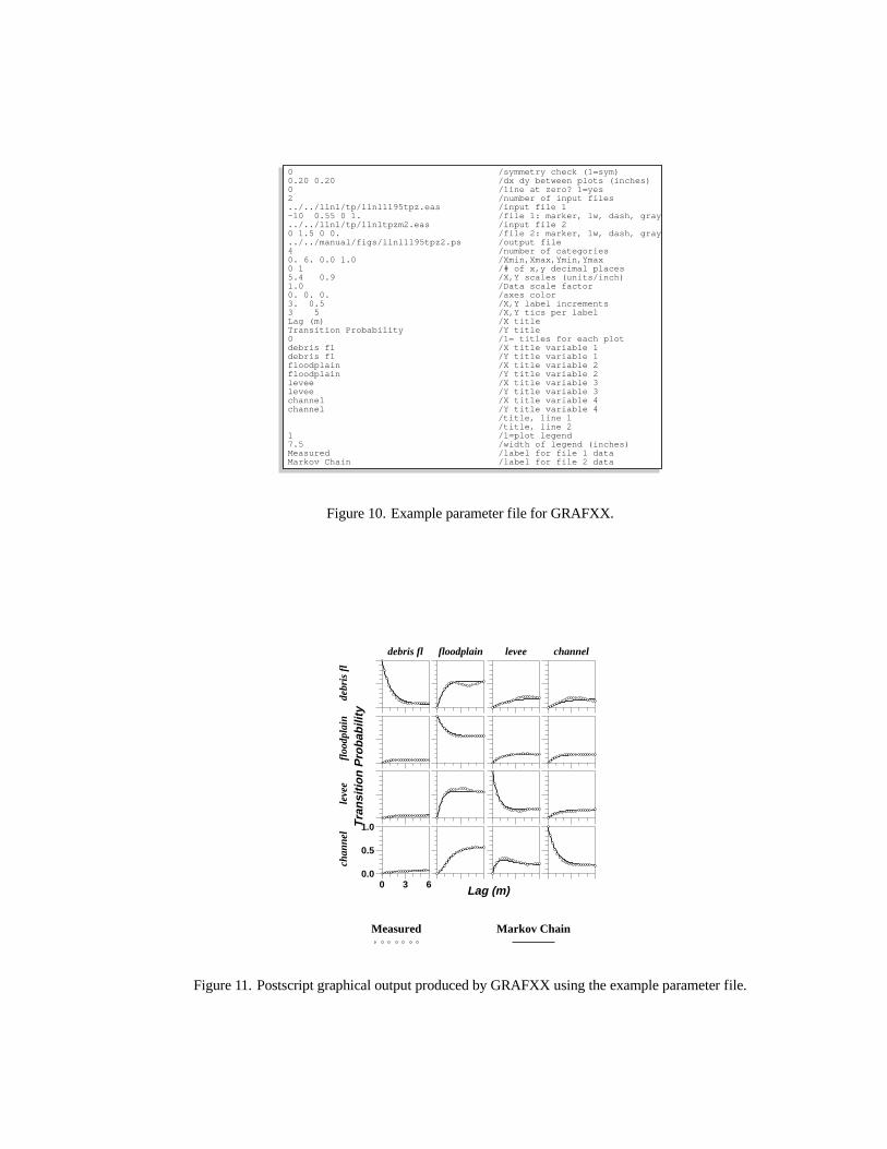
0 /symmetry check (1=sym)0.20 0.20 /dx dy between plots (inches)0 /line at zero? 1=yes2 /number of input files../../llnl/tp/llnl1195tpz.eas /input file 1-10 0.55 0 1. /file 1: marker, lw, dash, gray../../llnl/tp/llnltpzm2.eas /input file 20 1.5 0 0. /file 2: marker, lw, dash, gray../../manual/figs/llnl1195tpz2.ps /output file4 /number of categories0. 6. 0.0 1.0 /Xmin,Xmax,Ymin,Ymax0 1 /# of x,y decimal places5.4 0.9 /X,Y scales (units/inch)1.0 /Data scale factor0. 0. 0. /axes color3. 0.5 /X,Y label increments3 5 /X,Y tics per labelLag (m) /X titleTransition Probability /Y title0 /1= titles for each plotdebris fl /X title variable 1debris fl /Y title variable 1floodplain /X title variable 2floodplain /Y title variable 2levee /X title variable 3levee /Y title variable 3channel /X title variable 4channel /Y title variable 4 /title, line 1 /title, line 21 /1=plot legend7.5 /width of legend (inches)Measured /label for file 1 dataMarkov Chain /label for file 2 data
Figure 10. Example parameter file for GRAFXX.
Lag (m)
Tra
nsi
tio
n P
rob
abili
tyde
bris
fl
floo
dpla
inle
vee
debris fl
chan
nel
0 3 60.0
0.5
1.0
floodplain levee channel
Measured Markov Chain
Figure 11. Postscript graphical output produced by GRAFXX using the example parameter file.

Line Description1 a flag: 0 = display full matrix, 1 = show only lower triangle (if symmetric)2 X,Y spacing in inches between each of the graphs (matrix entries)3 a flag: 1 indicates put a horizontal line the ordinate (Y-axis) value of zero4 number of input files (data sets)5 1st input file name: e.g., a data file of vertical transition probabilities6 line attributes, file 1: marker, width (72/inch), dash, and gray (0=black, 1=white).7 2nd input file name: e.g., a Markov chain model8 line attributes, file 2:9 encapsulated PostScript output file name:tpz.eps10 number of categories11 X minimum, X maximum, Y minimum, Y maximum values for graphs12 number of decimal places in X, Y labels13 X, Y scales inunits per inch14 data scale factor (multiplier)15 axes gray level (0.0 = black, 1.0 = white)16 X, Y label increments17 X, Y tics per label18 X axis title19 Y axis title20 flag: 0 = column-row (X-Y) titles; 1 = titles for each graph21 to 28 column 1, row 1, ..., column 4, row 4 titles29 title, line 130 title, line 231 flag: 1 = plot legend32 width of legend in inches33 label for file 1 data34 label for file 2 data
Table 5. Description of parameters for GRAFXX.

24 Chapter 6 MCMOD
Dash Code
The dash code (used in the line attributes for lines 6 and 8 in Table 5) specifies the type of dashused in drawing a line that connects data.
0 = no dash1 to 10 = dash size proportionate to number
Marker Code
The marker code (used in the line attributes for lines 6 and 8 in Table 5) specifies the type ofmarker used to plot a data point.
Code Result0 line with no markersnegative markers with no linepositive markers and line÷1 cross÷2 diamond÷3 û÷4 box÷5 3-point star÷6 triangle÷7 5-point star÷8 pentagon÷9 6-point star÷10 circle÷11 sphere÷12 filled circle
If the marker code is zero (0), only a line connecting the data values is plotted. If the markercode is negative, say (-10), the data values are plotted as circles with no connecting lines. If themarker code is positive, say (+10), the data values are plotted as circles with connecting lines.

6 MCMOD
MCMOD provides several means for generating 1-D and 3-D Markov chain models of spatialvariability. The Markov chain is an important theoretical model for cross-correlated categori-cal variables. It has shown remarkable applicability to many categorical geological data sets,particularly vertical stratigraphic successions. Three-dimensional Markov chain models aregenerated inMCMOD by interpolating models for each of the principal directions, say%, +,and5 or stratigraphic strike, dip, and vertical (upward).
Before running MCMOD, the user must:
1. Have a rudimentary understanding of the transition probability and Markov chain models.
2. Set up a parameter file.
3. Check the array dimension settings in themcmod.inc include file.
4. If using option 2 (see below), prepare a GEOEAS-formattransition probabilitydata file (ascalculated fromGAMEAS ).
The resulting 3-D Markov chain file in binary grid format is used to prescribe the model ofspatial variability for the conditional simulation programTSIM (Chapter 7).
Theory
Markov chain models applied to time series assume that the future depends on the present andnot the past. For a one-dimensional spatial application, a Markov chain model assumes thatan outcome at a specified location depends entirely on the nearest datum. A three-dimensionalMarkov chain model assumes that spatial variability in any one direction can be characterizedby a one-dimensional Markov chain (Lin and Harbaugh, 1984; Politis, 1994). Although theMarkov chain is defined very simply in theoretical and mathematical terms, it has shown re-markable applicability to characterization of spatial variability of facies (or hydrostratigraphicunits) in alluvial and fluvial depositional systems (Carle and Fogg, 1996; Carle 1996; Carle andFogg, 1997; Carle and others, 1998). Mathematically, it can be shown that the Markov chainconsists of linear combinations of exponential structures, although non-exponential-looking‘‘Gaussian’’ and ‘‘hole-effect’’ structures can be generated.
Matrix Exponential Form
Mathematically, a Markov chain model applied to one-dimensional categorical data in a direc-

26 Chapter 6 MCMOD
tion è assumes amatrix exponentialform
AEûèä ' i T E+èûèä (6)
whereûè denotes a lag in the directionè, and+è denotes a transitionrate matrix
+è '
57 o��cè ü ü ü o�gcè...
......
og�cè ü ü ü oggcè
68with entriesoæ&cè representing the rate of change from categoryæ to category& (conditional tothe presence ofæ) per unit length in the directionè (Krumbein, 1968).
An eigenvalue analysismust be carried out in order to evaluatei T E+èûèä, because thematrix exponential isnot computed merely by computing the exponential of the matrix entries,that is,|æ&cèEûèä 9' i T Eoæ&cèûèä. Lettingû ' ûè and+ ' +è for notational simplification,i T E+ûä is either approximated by an infinite series or, better yet, exactly determined by
i T E+ûä 'g[ð'�
i T Ebðûä~ð
wherebð and~ð denote the eigenvalues and spectral component matrices, respectively, of+.The mathematical details are given in Agterberg (1974) and Carle and Fogg (1997) and Carleand others (1998). One eigenvalue, saybð, is inherently zero and is associated with a spectralcomponent matrix having the proportions along each column. Thus, for a four-category system,the continuous lag Markov chain model written out completely consists of
i T E+ûä ' E�éfä
5997R� R2 Rô ReR� R2 Rô ReR� R2 Rô ReR� R2 Rô Re
6::8n i TEb2ûä
59975��c2 5�2c2 5�ôc2 5�ec252�c2 522c2 52ôc2 52ec25ô�c2 5ô2c2 5ôôc2 5ôec25e�c2 5e2c2 5eôc2 5eec2
6::8 (7)
ni TEbôûä
59975��cô 5�2cô 5�ôcô 5�ecô52�cô 522cô 52ôcô 52ecô5ô�cô 5ô2cô 5ôôcô 5ôecô5e�éô 5e2cô 5eôcô 5eecô
6::8n i TEbeûä
59975��ce 5�2ce 5�ôce 5�ece52�ce 522ce 52ôce 52ece5ô�ce 5ô2ce 5ôôce 5ôece5e�ce 5e2ce 5eôce 5eece
6::8where the5kqcð are coefficients of the spectral component matrices~ð determined in the eigen-system analysis. Thus, the Markov chain model for each entry|æ&Eûä in AEûä consists of alinear combinationofg ý � exponential structures added to the column category proportion.For example, in the four-category case given in (7)
|æ&Eûä ' R& n 5æ&c2 i TEb2ûä n 5æ&cô i TEbôûä n 5æ&ce i TEbeûä

Theory 27
Comparison to Discrete-Lag Form
Markov chain models are often formulated by the ‘‘discrete-lag’’ approach by successive mul-tiplication of a transition probability matrixAE{ûèä at discrete lag{ûè
AE�{ûèä ' WAE{ûèäAE2{ûèä ' AE{ûèäAE{ûèä
...AE?{ûèä ' AdE?ý �ä{ûèoAE{ûèä
(8)
whereAEfä ' W. The discrete-lag approach generates transition probabilities at only discretelag multiples�{ûèc 2{ûèc éééc ?{ûè. However, any discrete-lag Markov chain can be con-verted to a continuous-lag Markov chain by computing
+è '*? dAE{ûèäo
{ûè(9)
which involves an eigensystem analysis (Agterberg, 1974; Carle, 1996; Carle and Fogg, 1997).
Eigensystem Analysis
MCMOD performs an eigensystem analysis because development of a continuous-lag Markovchain as a geostatistical model of spatial variability may require the following mathematicalcalculations:
î evaluate thematrix exponentialform of Markov chain given by (6),
î evaluate thematrix logarithmof a transition probability matrix given by (9), and
î convert a discrete-lag Markov chain to a continuous-lag Markov chain by combining (6)and (9).
As shown above, (6) and (9) cannot be computed directly from the matrix entries. In eithersituation, the key step is to find the eigenvalues of+è orAEûèä, which can be computed usingcodes for real general matrices as given by Smith and others (1976) or Press and others (1992).
For notational simplicity, let lagû ' ûè and+ ' +è. A square (g ûg) matrix such as+can be expressed in diagonal form with respect to its eigenvalues by
+ 'g[&'�
b&~& (10)
where theb& for & ' �c éééc g denote the eigenvalues of+, and~& denotes a spectral compo-nent matrix associated with each eigenvalueb&. The spectral component matrices~& can bedetermined directly from the eigenvalues and matrix+ by
~& '
T6õ'&
Eb6Wý+äT6 õ'&
Eb6 ý b&ä & ' �c éééc g (11)

28 Chapter 6 MCMOD
whereW denotes the identity matrix. The continuous-lag Markov chain (6) then can be computedfrom
A Eûä 'g[&'�
i T Eb&ûä~& (12)
through application of Sylvester’s theorem (Agterberg, 1974, p. 406-412). The value of oneeigenvalue of+ will be zero, and the remaining eigenvalues will be negative (to ensure thenegative diagonal transition rates). Recognizing that (12) represents a canonical form ofA Eûä,two useful conclusions can be drawn for the Markov chain model:
1. The eigenvaluesw&Eûä of AEûä relate to the eigenvaluesb& of + by
w&Eûä ' i T Eb&ûä or b& '*? w&Eûä
û;& ' �c éééc g (13)
2. Both+ andAEûä have identical spectral component matrices~&.
As a result, if a Markov chain model is assumed, a transition probability matrixAE{ûä fora discrete lag{û can be used to compute+ by applying (13) to (10) to obtain
+ 'g[&'�
*? w&E{ûä
{û~& (14)
wherew&E{ûä and~& are the eigenvalues and spectral component matrices, respectively, cor-responding toAE{ûä. Application of (14) to (6) yields
AEûä 'g[&'�
w&E{ûäû*{û~& (15)
which represents a continuous-lag version of the more commonly used discrete-lag Markovchain model (8). The clear advantage of (15) over (8) is the continuous functional representa-tion of the model, that is, the ability to calculateAEûä at anyû, not just integer multiples of{û. Expression (12) shows that a Markov chain model corresponds to a linear combination ofexponential functions. Nonetheless, rather nonexponential looking structures can be obtainedfrom a Markov chain model, as evident in some of the off-diagonal transition probabilities forthe examples given.
Considering that one eigenvalue of+, sayb�, has a value of zero, the corresponding eigen-valuew�Eûä of AEûä has a value of unity for allû. The entries of the spectral component matrix~� correspond to the proportionR& of the column category such that
~� '
57 R� ü ü ü Rg...
...R� ü ü ü Rg
68Considering (12) and that the other eigenvaluesb2c éééc bg are negative such that*ð4
û<"i TEb&ûä '
f for & ' 2c éééc g, then~� establishes the sill of the Markov chain model as given by (5).

Theory 29
Properties
The transition rate matrix has some important theoretical properties useful in model develop-ment:
î The transition rate corresponds to theslopeof the transition probability as it approaches lagzero
oæ&cè 'Y|Eü$ fä
Yûè(16)
î The diagonal entries are negative (oææcè ÷ f), and the off-diagonal entries are (usually)non-negative (oæ&cè è f ;& 9' æ), which ensures thatf é |æ&Eûèä é �.
î The diagonal entriesoææcè are related touæcè, the mean length of categoryæ in the directionè, by
oææcè ' ý �
uæcè(17)
For example, the mean ‘‘thickness’’ [mean length in the vertical (5) direction] of categoryæcorresponds touæc5, so that a diagonal transition rateoææc5 can be established by
oææc5 ' ý �
uæc5
î The row sums must equal zero
g[&'�
oæ&cè ' f ;æ (18)
such that the diagonal entry is equivalent to the negative of the sum of the off-diagonal rowentries
oææcè ' ýg[& õ'æ
oæ&cè ;æ
which ensures thatgS& õ'æ
|æ&Eûèä ' � for all æc & according to probability law.
î The column sums must obey
g[æ'�
Ræoæ&cè ' f ;& (19)
which ensures that the transition matrix converges on the specified proportions,|æ&Eûè $4ä ' R&, as expected for a stationary Markov chain.
Background Category
Probability law and knowledge of proportions can be exploited inMCMOD by specifying

30 Chapter 6 MCMOD
one category as ‘‘background.’’ Usually proportions are knowna priori, such that the row andcolumn summing constraints (18) and (19) can be applied to eliminate the need to specify onecolumn and one row of transition rates. For example, in a four-category system, onlyôûô ' btransition rates need to be established instead ofeû e ' �Sé
Multidimensional Markov Chains
2-D or 3-D Markov chain models can be developed by assuming that spatial variability in anydirection can be characterized by a 1-D Markov chain (Switzer, 1965; Lin and Harbaugh, 1984;Politis, 1994). Although this may seem like a tenuous theoretical leap, the assumption hereis merely that Markov chains might characterize spatial variability not only in the vertical butin other stratigraphic directions such as dip or strike. In a typical geologic application, datacoverage usually is inadequate to directly develop a 1-D Markov chain model for each of theinfinity of directions. Alternatively, model development can focus on the principal directions,say the strike (%), dip (+) and vertical (5). Then 1-D Markov chain models for any directioncan be interpolated from the principal direction models.2
Considering that the transition probability matrixAEûèä for an arbitrary directionè dependsentirely on+è, the interpolation of Markov chain models can be accomplished by ellipsoidallyinterpolating entries in the transition rate matrices for the principal%c + and5 directions by
moæ&cè m 'vë
û%ûèoæ&c%
ê2
n
ëû+ûèoæ&c+
ê2
n
ëû5ûèoæ&c5
ê2
;æc & 9' q (20)
whereq denotes the background category,û%c û+ andû5 are the%c + and5 direction componentsof ûè '
sû2% n û
2+ n û
25. The remaining entries in+è involving æ or & ' q can be determined
by applying (18) and (19). For the negative lag vector components, sayû3%, entries from therate matrix+3% corresponding to the opposite directioný% are defined by
oæ&c3% 'ëR&Ræ
êo&æc%
and used in (20) in place of entries for+%, in accordance with the backward Kolmogorovdifferential equation (Agterberg, 1974, p. 455-456).
The Determinant - A Measure of Statistical Closeness
The lateral extent of the 3-D Markov chain model output byMCMOD must be finite, with lim-its that consider statistical closeness. Kriging-based algorithms, which do not consider cross-correlations, easily rank statistical closeness by the magnitude of the variogram (or covariance)model or a prescribed search radius with anisotropy ratios. However, the ranking of a fullcross-correlation matrix for multiple categories is not so straightforward.
2 We make no claim that non-negative definiteness is guaranteed for the three-dimensional Markov chain models. However, 1-D non-negative definiteness is ensured for each of the principal directionè models by maintaining real and non-positive eigenvalues for+è. Ourexperience has shown that the transition probability-based cokriging equations implemented in TPSIM, although singular, are solvable bysingular value decomposition.
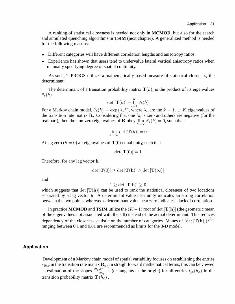
Application 31
A ranking of statistical closeness is needed not only inMCMOD , but also for the searchand simulated quenching algorithms inTSIM (next chapter). A generalized method is neededfor the following reasons:
î Different categories will have different correlation lengths and anisotropy ratios.
î Experience has shown that users tend to undervalue lateral:vertical anisotropy ratios whenmanually specifying degree of spatial continuity.
As such, T-PROGS utilizes a mathematically-based measure of statistical closeness, thedeterminant.
The determinant of a transition probability matrixAEûä, is the product of its eigenvaluesw&Eûä
_i| dAEûäo 'g
á&'�
w&Eûä
For a Markov chain model,w&Eûä ' i T Eb&ûä, whereb& are the& ' �c éééc g eigenvalues ofthe transition rate matrix+. Considering that oneb& is zero and others are negative (for thereal part), then the non-zero eigenvalues of+ obey *ð4
û<"w&Eûä ' f, such that
*ð4û<"
_i| dAEûäo ' f
At lag zero (û ' f) all eigenvalues ofAEfä equal unity, such that
_i| dAEfäo ' �
Therefore, for any lag vectorü
_i| dAEfäo è _i| dAEüäo è _i| dAE4äo
and� è _i| dAEüäo è f
which suggests that_i| dAEüäo can be used to rank the statistical closeness of two locationsseparated by a lag vectorü. A determinant value near unity indicates an strong correlationbetween the two points, whereas as determinant value near zero indicates a lack of correlation.
In practiceMCMOD andTSIM utilize theEgý�ä root of_i| dAEüäo (the geometric meanof the eigenvalues not associated with the sill) instead of the actual determinant. This reducesdependency of the closeness statistic on the number of categories. Values ofE_i| dAEüäoä
�g3�
ranging between 0.1 and 0.01 are recommended as limits for the 3-D model.
Application
Development of a Markov chain model of spatial variability focuses on establishing the entriesoæ&cè in the transition rate matrix+è. In straightforward mathematical terms, this can be viewedas estimation of the slopesY|æ&Eü<fä
Yûè(or tangents at the origin) for all entries|æ&Eûèä in the
transition probability matrixA Eûèä é

32 Chapter 6 MCMOD
Selecting the Background Category
As stated above, application of the background category concept eliminates the need to specifyone row and column of transition rates. In general, the background category may be selectedaccording to geologic interpretation as the category that fills in the space not occupied by othercategories. For example, in a fluvial depositional system consisting oflag, channel, levee, andflood plain deposits, theflood plain facies would be a logical choice for background because ithas the lowest energy of deposition and, therefore, fills in accommodation space not otherwiseoccupied by higher energy facies.
Choosing the Approach
MCMOD can generate one-dimensional Markov chains by either (1) direct quantitative means,(2) estimation ofY|æ&Eü<fä
Yûècorresponding to the slope of the transition probability as lag ap-
proaches zero, (3) direct fitting to data, or (4) interpretation of juxtapositional tendencies. As aresult, five different modeling approaches can be implemented withMCMOD :
1. Transition Rates – Prescribe the actual transition rates.
2. Discrete Lag– Honor transition probability data for a particular (discrete) lag .
3. Embedded Transition Probabilities – Interpret transition rates relative to an embeddedtransition probability matrix.
4. Embedded Transition Frequencies– Interpret transition rates relative to an embeddedtransition frequency matrix.
5. Independence- Interpret transition rates relative to ‘‘independent’’ or ‘‘maximum entropy(disorder)’’ juxtapositional tendencies.
The choice of approach will depend on the particular application or style of interpretation.The fact that many approaches are available exemplifies the flexibility of the Markov chain asa model of spatial variability. Various modeling situations are given below, for which the mostconducive approaches are recommended.
Sparse Data
Most practical data sets yield noisy looking transition probability (or indicator cross-variogram)measurements, particularly for the lateral directions. The traditional geostatistical model devel-opment approach of empirical curve-fitting can easily lead to overcomplicated structures andinconsistencies with mathematical and probability theory. Alternatively, the Markovian modelsoundly addresses mathematical and probability theory while offering an interpretive frame-work for defining model parameters. The assumption of a Markov chain may be viewed asa conceptual simplification, that the spatial variability depends on values at nearest locations(first-order stochastic). One can develop a Markov chain (first-order) model from parametersconducive to integration of geologic insight: proportions, mean length, and juxtapositional ten-dencies. Noisy data typically do not support a more complicated (higher-order) model, unlesssupported by ancillary or interpretive information.

Application 33
Recommendation:Embedded Transition Probabilities- Prescribe cross (off-diagonal) transition rates in terms of conditionalprobabilities of embedded occurrences. For example, ‘‘Given an embedded occurrence of clay, what is theprobability that sand occurs directly above?’’ Prescribe auto (diagonal) transition rates by mean lengths.Transition Rates - Infer the slope or fit (interpolate) the tangent line of transition probability curve as
lag approaches zero as per (16); these slope values directly translate to transition rates. Use this approachin conjunction with the embedded transition probability approach (through examination of the debuggingfile) to infer whether the prescribed transition rates are geologically plausible.
No Data
The Markovian framework is particularly conducive to development of models of spatial vari-ability from conceptual information and, thus, is well-suited to situations lacking any data at all.For example, one can use geologic information or other insights on facies proportions, meanlengths, and juxtapositional tendencies to establish a geologically plausible model of spatialvariability.
Recommendation:Embedded Transition Probabilities - Prescribe cross-transition rates by estimating conditional proba-
bilities of embedded occurrences according to geologically plausible juxtapositional tendencies. Prescribeauto-transition rates by estimated mean lengths.
Abundant Data
Given abundant data, the measured transition probabilities may display Markovian propertiesand define a smooth curve (without scatter). This situation might occur for numerous, finely-spaced data, such as continuous logs obtained from multiple boreholes penetrating the samegeologic system.
Recommendation:Discrete Lag– Use transition probability data at one (discrete) lag to establish the model at all lags.Transition Rates– Infer the slope of the transition probability as the lag approaches zero; the slope valuesdirectly translate to transition rates as indicated by (16).
Interpretation Relative to Statistical Independence or Maximum Entropy (Disorder)
A main motivation for performing statistical analysis of bedding successions has been to quan-tify interpretation of juxtapositional tendencies, to address questions such as, ‘‘Does siltstonetend to occur above sandstone (versus claystone or conglomerate).’’ A standard is needed forjudging whether a juxtapositional tendency is greater or lesser than ‘‘random.’’ This can bebased on statistical ‘‘independence,’’ for which the frequency of occurrence of a pairs of eventsdepends on the product of the marginal frequencies of the two events. Theoretically, statisticalindependence is identical to the maximum entropy concept, wherein a spatial arrangement of agiven number of categories exhibits a state of maximum disorder.
Recommendation:Independence– Set cross-transition rates relative to the independent (maximum entropy) model. Set
auto-transition rates according to mean lengths. Use this approach primarily to interpret whether the dataor model exhibit significantly nonrandom juxtapositional tendencies.

34 Chapter 6 MCMOD
Transition Frequency/Count Data
The raw data used in an embedded Markov chain analysis consists of transition counts, for ex-ample, the number of observations of siltstone occurring over sandstone. These values may benormalized by the sum of the entire matrix to obtain transition frequencies, or the row sum toobtain transition probabilities. Recall that transition frequencies, rather than transition prob-abilities, are used in the assessment of statistical independence and, thus, represent a morefundamental statistic.
Recommendation:Transition Frequencies– Prescribe transition frequencies or counts for off-diagonal entries, mean lengthsfor diagonal entries.
Direct Quantitative Interpretation
Transition rates can be interpreted directly in terms of a conditional rate of change per unitlength. The auto-transition rates are negative because the auto-transition probability at an in-finitesimal lag is less than unity (the auto-transition probability at lag zero). Similarly, thetransition rates to other categories are usually positive because the cross-transition probabili-ties at an infinitesimal lag are expected to be greater than zero (the cross-transition probabilityat lag zero). Specifically,oæ&cè denotes, given an occurrence ofæ, the rate at whichæ transitionsto & per unit length in a directionè. For example, ifæ is very continuous in the directionè (æpossesses a very large mean length),oææcè will be negative and very small in magnitude, andoæ&cè for & 9' æ will be positive but smaller in magnitude thanoææcè, particularly if& tends notto occur adjacent toæ. The summing constraint (18) maintains adherence to probability law byprescribing that the auto-transition rates equal the negative of the sum of the cross-transitionrates.
Recommendation:Transition Rates– Directly prescribe transition rates in terms of conditional rate of change per unit lengthor by estimation of the slopesCwmn+k$3,Ck!
(or tangents at the origin).

Application 35
Description of Approaches
1. Transition Rates
The transition rates are the entriesoæ&cè in +è of the equation describing a continuous-lagMarkov chain (6). The transition rates can be interpreted as the slope of the tangent of thetransition probability curve as the lag approaches zero, as indicated by (16). Thus, one approachto developing a transition rate matrix would be to estimate the slopesY|æ&Eü<fä
Yûèindicated by
transition probability data. For example, a 4-category (debris flow, floodplain, levee, channel)vertical transition rate matrix could be established as
+5 '
5997ýféH. ú fé�f féfSSú ú ú ú
féfôf ú ý�é2ô fé�2féfôb ú fé.b ýféH2
6::8m3� (21)
by estimation of the slopesY|æ&Eü<fä
Yûè. Recall that row and column sums of+è should obey (18)
and (19), which can be achieved by employing the background category concept. The entriesfor the row and column involving category 2, the background category, need not be specified.Note that the diagonal entries are negative, and the off-diagonal entries are non-negative. Toavoid negative or above-unity probabilities, these sign conventions are recommended! Figure12 shows the Markov chain model resulting from this transition rate matrix.
2. Discrete-lag Approach using Transition Probability Data at a Particular Lag
MCMOD employs an eigensystem analysis of (9) to establish a transition rate matrix fromtransition probability data at a particular lag, where{ûè would be chosen within the range ofcorrelation. For example, the vertical (5)-direction transition probability matrix
AE{û5 ' féS mä '
5997féS�H2 fé2Hb2 féfD2b féfôb.féfô2D féHfS� féf.H. féfH2Sféf�b2 féôH�. féD2DH féf.2.féf�SH féfbbD fé2ôDb féSe.H
6::8was used to compute the transition rates in (21) by (9) to obtain the model shown in Figure 12.
3. Transition Probabilities of an Embedded Markov Chain Analysis
An embedded Markov chain analysis evaluates the conditional probabilities of discrete occur-rences of geologic units occurring adjacent to others in a particular direction (see Figure 2). Forexample, theembeddedtransition probabilitiesZæ&c5 in the vertical (5) direction are defined as
Zeôc5 ' èh i,eñee occurs abovem Sû@??e, occurs belowj

36 Chapter 6 MCMOD
Lag (m)T
ran
siti
on
Pro
bab
ility
debr
is f
lfl
oodp
lain
leve
e
debris fl
chan
nel
0 3 60.0
0.5
1.0
floodplain levee channel
Measured Markov Chain
Figure 12. Matrix of transition probability data fit by Markov chain using discrete-lag approach at 0.6 m lag.
Consequently, an embedded transition probability matrixá5 could be constructed as
á5 '
5997ý féHfô fé�2e féf.ô
fé�.S ý féôbf féeôeféf2S féHeS ý fé�2HféfeD féfDH féHbS ý
6::8 (22)
Note that auto (diagonal)-transitions are considered unobservable, thus, the diagonal entries areabsent. From an interpretive standpoint, note in (22) thatZeôc5 :: Ze�c5 andZeôc5 :: Ze2c5,which indicates thatleveetends to occur abovechannel.
With the additional information of mean lengthuæc5, the entries of an embedded transitionprobability matrix can be translated into entries in a transition rate matrix by
oæ&c5 'Zæ&c5
uæc5(23)
The transition rates in (21) are related to the embedded transition probabilities in (22) by (23).Thus, one approach to developing a transition rate matrix can be to (a) establish an embeddedtransition probability matrix from either data or geologic interpretation of juxtapositional ten-dencies, (b) establish mean lengths, and (c) convert the embedded transition probabilities totransition rates by (23).
Note that the off-diagonal entriesoæ&c5 defined by (23) satisfy (17) and (18) because
g[&'�
Zæ&c5 ' �
If a background category is assumed,the row and column entries involving the background

Application 37
Lag (m)T
ran
siti
on
Pro
bab
ility
debr
is f
lfl
oodp
lain
leve
e
debris fl
chan
nel
0 3 60.0
0.5
1.0
floodplain levee channel
Measured Markov Chain Max. Entropy
Figure 13. Markov chain model fit to matrix of transition probability measurements by using option 3 toadjust embedded transition probabilities. Markov chain model based on independent or ‘‘maximum entropy’’juxtapositional tendencies shown by dashed line.
category do not need to be specified(set them to zero). A revised+5 was established fromembedded transition probabilities and mean lengths by5997
u�c5 ' �é�D ú fé�2 féf.Dú ú ú ú
féf2D ú uôc5 ' féH2 fé�fféfe ú fébS uec5 ' �é2e
6::8 (24)
where the diagonal entries are converted to transition rates by (17), the off-diagonal entries areconverted to transition rates by (23), and category 2 is assumed as background (why row 2 andcolumn 2 entries are set to any number). The resulting Markov chain model shown in Figure13 fits the transition probability measurements slightly better than the initial model shown inFigure 12.
4. Transition Frequencies of an Embedded Markov Chain Analysis
An embedded Markov chain analysis may also be performed in terms of embedded transitionfrequenciessæ&cè defined, for example in the vertical (5) direction, as
seôc5 ' èh i,eñee occurs above andSû@??e, occurs belowj

38 Chapter 6 MCMOD
An embedded transition frequency matrix65 could be formulated as
65 '
5997EféfHe�ä féfS.. féf�f� féffSôféfS.2 EféôeSHä fé�2Se fé�.�ôféffHD fé2b.� EféôôbDä féfôefféffHD féffff fé2fô� Efé2��Dä
6::8where the diagonal entries (in parenthesis) are the row and column sums corresponding to mar-ginal frequenciessæc5 of embedded occurrences of categoryæ
sæc5 'g[& õ'æ
sæ&c5 'g[& õ'æ
s&æc5 (25)
With the additional information of mean lengthuæc5, the transition frequencies can be con-verted to transition rates by
oæ&c5 'sæ&c5
sæc5uæc5;& 9' æ (26)
Analogous to (24),MCMOD can establish the rate matrix from transition frequencies inthe off-diagonal entries by5997
u�c5 ' �é�D ú féf�f� féffSôú u�c5 ' 2é2.é ú ú
féffHD ú uôc5 ' féH2 féfôefféffHD ú fé2fô� uec5 ' �é2e
6::8Although off-diagonal entries for the background row and column do not need to be speci-fied, this approach requires a mean length for the background categorybecause the marginalfrequencies depend on the proportions and mean lengths for all categories.
5. ‘‘Independent’’ or ‘‘Maximum Entropy’’ (Disorder) Transition Frequencies
The juxtapositional tendencies in a geologic system reflect some degree of order (or disorder)in the bedding sequences. The disorder of the juxtapositional tendencies in a particular direc-tion, sayè, can be quantified by the entropy7è of bed-to-bed transition frequenciessæ&cè, theprobabilities that one bed occurs next to another, by
7è ' ý[æ
[&
sæ&cè *? sæ&cè (27)
(Hattori, 1976). Consider the question, ‘‘What would the bedding look like for a maximally dis-ordered system?’’ From this state of reference, one might be able to judge whether the observedbedding sequence exhibits nonrandom juxtapositional tendencies, that is, some preferentialor-der.
In applyingembeddedMarkov chain analyses, geologists have been interested in quantify-ing their interpretations of facies successions, particularly in the vertical direction. ‘‘Random’’or independent transition frequencies for a succession involving four categories of beds would

Application 39
obey 5997s�s� s�s2 s�sô s�ses2s� s2s2 s2sô s�sesôs� sôs2 sôsô sôseses� ses2 sesô sese
6::8 (28)
wheresð denotes the ‘‘marginal’’ frequency that a bed of categoryð occurs in the succession (thedirectionè is implied for notational simplicity). However, the problem is not so straightforwardin practice. Usually, self-transitions (between two beds of the same category) are unobservable(particularly from borehole data), so that not only the diagonal transition frequencies but alsothe marginal frequencies cannot be directly evaluated. Off-diagonal transitioncountscan beestimated accurately, because transitions from one category to adifferent category are observ-able.
Assuming that self-transitions are unobservable, a more practical problem is posed. Instead,one analyzes observations of off-diagonal transition frequencies#æ&, which are defined as thetransition counts divided by the sum total of all the off-diagonal transition counts5997
ý #�2 #�ô #�e#2� ý #2ô #2e#ô� #ô2 ý #ôe#e� #e2 #eô ý
6::8Self-transitions are unobservable, so the diagonal entries are left blank. The objective of theindependent transition frequencies (Turk, 1979; Turk, 1982; Johnson and Pattie, 1993) is to findthesð’s that satisfy
�
A
g[æ õ'ð
sðsæ 'g[æ õ'ð
#ðæ ;ð ' �c éécg (29)
whereA 'gSð'�
gSæ õ'ðsðsæ. The non-linear system of equations (29) can be solved by the method
of iterative proportion fitting (IPF) (Johnston and Pattie, 1993; Carle, 1997a). The resultingindependent model will display the same marginal frequencies ofembeddedoccurrences#ð,where
#ð 'g[æ õ'ð
#ðæ ;ð ' �c ééc g
The off-diagonal transition frequencies will be independent with respect to the estimatedsð’s.Continuous lag Markov chain models can be linked to this model of independency by notingthat#ð is proportional to proportionsRð divided by mean lengthuð such that
Rðuð2 #ð ;ð ' �c ééécg
Thus, given a set of proportions and mean lengths, a continuous lag Markov chain with inde-pendent transition frequencies can be derived.
So a more specific question arises, ‘‘For the given proportions and mean lengths, what isthe transition frequency matrix that maximizes entropy as defined in (27) ?’’ It so happensthat the concept of statistical independence yields the same result as maximum entropy. The

40 Chapter 6 MCMOD
resulting independent or maximum entropy transition frequency matrix6E74@ ä5 corresponding
to the proportions and mean lengths of the previous examples is
6E74@ ä5 '
5997EféfHe�ä féfô.. féfô�� féf�D2féfô.. EféôS.�ä fé2�bS fé�f.Dféfô�� fé2�bS EféôôbSä féfHHHféf�D2 fé�f.D féfHHH Efé2��Dä
6::8where the diagonal entries represent the row/column totals or marginal frequencies. This matrixcan be used as a basis for interpretation of juxtapositional tendencies relative to a maximallydisordered bedding succession for the same proportions and mean lengths. For example, if anobserved transition frequencyseôc5 is greater thans E74@ ä
eôc5 , then one might conclude that thereis a statistical tendency forleveeto occur abovechannel.
One can develop a transition rate matrix by (a) establishing proportions and mean lengths,(b) computing the maximum entropy transition frequency matrix6
E74@ ä5 and corresponding
transition rates, and (c) interpreting the off-diagonal transition rates relative to the maximumentropy transition rates. For example, applying (26), a maximum entropy transition rateo
E74@ äæ&c5
can be computed by
oE74@ äæ&c5 '
sE74@ äæ&c5
uæc5S& õ'æ
sE74@ äæ&c5
The vertical transition rate matrix (21) can be formulated relative to the maximum entropytransition ratesoE74@ ä
æ&cè as
+E74@ ä5 '
59999973�
u�c5'�é�D m�éHfo
E74@ ä�2c5 féô2o
E74@ ä�ôc5 fée�o
E74@ ä�ec5
�é.HoE74@ ä2�c5
3�u2c5'2é2. m
féDHoE74@ ä2ôc5 �éDbo
E74@ ä2ec5
fé2.oE74@ äô�c5 �éôDo
E74@ äô2c5
3�uôc5'féH2 m
féeDoE74@ äôec5
féDSoE74@ äe�c5 féffo
E74@ äe2c5 2é2bo
E74@ äeôc5
3�uec5'�é2e m
6:::::8 (30)
By this approach off-diagonal transition rates are established by multiplyingoE74@ äæ&c5 by a co-
efficient: greater than unity indicates that the two categories tend to occur next to each other;lesser than unity indicates that the two categories tend not to occur next to each other.
The maximum entropy concept is particularly useful for interpreting juxtapositional ten-dencies of an existing Markov chain model. For example, one can take the proportions andmean lengths established by the existing model, say (21), then generate a Markov chain modelwith maximally disordered juxtapositional tendencies for those mean lengths and proportions(which establish the marginal frequencies of embedded occurrences). Comparison of transi-tion probability measurements with the maximum disorder model can then be used to interpretwhether the stratigraphy exhibits some degree of order in the juxtapositional tendencies.MC-MOD can be used to establish the maximum entropy Markov chain model, shown in Figure 13,

Parameter File 41
for the given proportions and mean lengths in the previous examples by specifying for option 55997u�c5 ' �é�D �éf �éf �éf
�éf u2c5 ' 2é2. �éf �éf�éf �éf uôc5 ' féH2 �éf�éf �éf �éf uec5 ' �é2e
6::8where setting the off-diagonal coefficients equal to unity yields the maximum-entropy transitionrates.The mean length must be specified for@,, categories including the background category.
The symmetric three-category case.In the special case of three categories with an as-sumption of symmetry, the maximum entropy system of equations reduces to 3 equations (therow/column summing constraints) and 3 unknowns (the symmetric off-diagonal transition fre-quencies). Therefore, the juxtapositional tendencies will always appear as ‘‘maximum entropy’’for the given proportions and mean lengths. This situation illustrates the possible conflict be-tween geological and statistical interpretations of maximum disorder. For example, considera system with three facies: channel, levee, and a large proportion of floodplain deposits. Ageologist would expect that levee deposits tend to occur laterally adjacent to the channel de-posits and not haphazardly throughout the floodplain. Conversely, the location of the leveedeposits could be viewed as tending to occur laterally adjacent to the floodplain deposits. Ifthe levee deposits did in fact occur haphazardly throughout the floodplain, the effect would beto reduce the mean length of the floodplain deposits, i.e. the floodplain deposits would be lesslaterally extensive. Thus, in a geologic interpretation of the relative disorder of juxtapositionaltendencies, one may also need to make comparisons of entropy allowing for one or more facies(particularly the background category) to vary in mean length.
Parameter File
The parameter file forMCMOD consists of four parts: (a) parameters common to the 3-D model, (b) parameters describing the%-direction model, (c) parameters describing the+-direction model, and (d) parameters describing the5-direction model. The formats describingeach%c +c 5-direction model are identical. Figure 14 shows an example parameter file for afour-category application using options 1 and 2. The parameters are described in further detailin Table 6. Figure 15 shows another example parameter file using options 3 and 4.

42 Chapter 6 MCMOD
Line Description1 number of categories2 proportions for each category (should add up to unity!)3 background category (highly recommended, but can be set at zero if not used)4 file name for debugging file5 file name for 3-D Markov chain model produced in binary grid (.bgr) format6 file name for determinant file used later inTSIM to determine statistical closeness7 {> |> } lateral extent of 3-D model in terms of determinant8 {> |> } lag spacing for 3-D model (same as for conditional simulation byTSIM )9 {-direction output file name for 1-D Markov chain model10 {-direction number of lags, lag spacing11 {-direction modeling approach (option 1 in this example)12 row 1 entries for{-direction transition rate matrix13 row 2 entries for{-direction transition rate matrix14 row 3 entries for{-direction transition rate matrix15 row 4 entries for{-direction transition rate matrix16 |-direction output file name for 1-D Markov chain model17 |-direction number of lags, lag spacing18 |-direction modeling approach (option 1 in this example)19 row 1 entries for|-direction transition rate matrix20 row 2 entries for|-direction transition rate matrix21 row 3 entries for|-direction transition rate matrix22 row 4 entries for|-direction transition rate matrix23 }-direction output file name for 1-D Markov chain model24 }-direction number of lags, lag spacing25 }-direction modeling approach (option 2 in this example)26 transition probability data file27 lag number for developing Markov chains from transition probability data
Table 6. Description of parameter file shown in Figure 13.
4 /# of categories0.066 0.565 0.190 0.179 /proportions2 /background category../llnl/tp/mcmod1_2.dbg /name of debugging file../llnl/tp/tpxyz1_2.bgr /output file for 3-D model../llnl/tp/det1_2.bgr /output file for determinant0.05 0.05 0.05 /determinant extent for 3-D model3.0 10.0 0.30 /dx,dy,dz for 3-D model../llnl/tp/llnltpxm1_2.eas /X-direction output file200 1. /X-Direction: # lags, spacing1 /option: 1=r,2=d,3=etp,4=etf,5=i -0.125 0. -1. -1. /row 1 transition rates 0. 0. 0. 0. /row 2 transition rates 0.0042 0. -0.167 -1. /row 3 transition rates 0.004 0. 0.084 -0.100 /row 4 transition rates../llnl/tp/llnltpym1_2.eas /Y-direction output file200 2.5 /Y-Direction; # lags, spacing1 /option: 1=r,2=d,3=etp,4=etf,5=i -0.042 0. 0.0036 0.0022 /row 1 transition rates 0.0 0. 0. 0. /row 2 transition rates 0.0013 0. -0.050 0.016 /row 3 transition rates 0.0008 0. 0.017 -0.020 /row 4 transition rates../llnl/tp/llnltpzm1_2.eas /Z-direction output file200 0.1 /Z-Direction: # lags, spacing2 /option: 1=r,2=d,3=etp,4=etf,5=i../llnl/tp/llnl1195tpz.eas /data file2 /lag#
Figure 14. Example parameter file for MCMOD using options 1 and 2.

Implementation Notes 43
4 /# of categories0.066 0.565 0.190 0.179 /proportions2 /background category../llnl/tp/mcmod3_4.dbg /name of debugging file../llnl/tp/tpxyz3_4.bgr /output file for 3-D model../llnl/tp/det3_4.bgr /output file for determinant0.05 0.05 0.05 /determinant extent for 3-D model3.0 10.0 0.30 /dx,dy,dz for 3-D model../llnl/tp/llnltpxm3_4.eas /X-direction output file200 1. /X-Direction: # lags, spacing3 /option: 1=r,2=d,3=etp,4=etf,5=i8.0 0. -1. -1. /row 1 embedded tp’s & ml’s0. 0. 0. 0. /row 2 ’’0.025 0. 6.0 -1. /row 3 ’’0.040 0. 0.84 10. /row 4 ’’../llnl/tp/llnltpym3_4.eas /Y-direction output file200 2.5 /Y-Direction; # lags, spacing4 /option: 1=r,2=d,3=etp,4=etf,5=i24. 0. -1. -1. /row 1 embedded tf’s & ml’s0. 62.81 0. 0. /row 2 ’’0.0095 0. 20.0 -1. /row 3 ’’0.0058 0. 0.1208 50. /row 4 ’’../llnl/tp/llnltpzm3_4.eas /Z-direction output file200 0.1 /Z-Direction: # lags, spacing3 /option: 1=r,2=d,3=etp,4=etf,5=i1.15 0. 0.12 0.075 /row 1 embedded tp’s & ml’s0. 0. 0. 0. /row 2 ’’0.025 0. 0.82 0.10 /row 3 ’’0.04 0. 0.96 1.24 /row 4 ’’
Figure 15. Example parameter file for MCMOD using options 3 and 4.
Implementation Notes
î Line 3 – If the background category is not used (set at zero), a 3-D model will not beproduced.
î Line 6 – The determinant is the product of the eigenvalues. For a Markov chain,_i| dAEfäo '� and_i| dAE4äo ' f. In general, try values ranging from 0.01 to 0.1 – the smaller the num-ber, the greater the lateral extent; the greater the lateral extent, the larger the array size forthe 3-D transition probability model, which, as stated earlier, is afive-dimensional array.The actual array size will depend on the Markov chain model parameters (primarily meanlength) and lag spacing (line 7).
î Line 7 – Anticipate thatTSIM will assume the lag spacing of the 3-D Markov chain modelis the same as the grid spacing for generating the realizations.MCMOD runs fast, so re-runningMCMOD with revised lag spacing is easily performed by editing line 7 as needed,without changing any other parameters. One should consider that reducing grid spacing inthe conditional simulations will necessitate increased array size for the 3-D Markov chainmodel. The determinant limit specification takes care of this adjustment automatically.
î 1-D files– The 1-D%c + and5-direction model files are produced independently of the 3-DMarkov chain model. Thus, very small lag spacings can be prescribed for the 1-D models,which are useful for graphing the models as continuous functions.
î Option 2 – If an option other than ‘2’ is chosen in line 25 as given in Table 6, the inputformat would replace lines 26-27 with four (g) lines describing the parameters of each rowof the transition rate matrix.
î Options 3 through 5– These options permit establishment of the transition rates by moreinterpretable methods than options 1 and 2. In each of these options, thediagonal transitionrates will be established indirectly by prescribing values ofmean length.

44 Chapter 6 MCMOD
î Background Category– The background category concept eliminates the need to specifyentries in the background category row and column, except for the diagonal (mean length)entry in options 4 and 5.
î Symmetry– One can enforcesymmetryin opposing pairs of off-diagonal transition rates bysetting oneof the opposing entries equal to negative unity (-1.0). Thus, if all juxtapositionaltendencies are assumed symmetric, one can focus on establishing transition rates for eitherthe lower or upper off-diagonal entries; the opposing off-diagonal entries can all be set to-1.0.
Include File
The file mcmod.inc is used to set the dimensions of arrays used inMCMOD . If not familiarwith the dimension settings, the user should checkmcmod.inc, reset dimensions (if necessary),and recompilemcmod.f(or).
Output
The output files ofMCMOD are a 3-D Markov chain model (line 5), which consists of a 5-Darray stored in the binary grid format, and a 3-D grid of determinant values (line 6). These twogrid files are used byTSIM for conditional simulation.
The one-dimensional%, +, and5-direction Markov chain model output files for (lines 9, 16,and 23) are generated independently of the 3-D model to enable interpretation and comparisonwith transition probability measurements along principal directions. It is recommended to gen-erate the one-dimensional models at small lag spacings (usually smaller than the grid spacingof the 3-D model) in order to adequately display the continuity of the Markov chain model.
Debugging File
After runningMCMOD , one should check the debugging file because it provides useful diag-nostic information on the principal-direction and 3-D Markov chain models as follows:
î options used
î actual transition rates
î transition rates in terms of the more interpretive frameworks of options 3 through 5.
î eigenvalue and spectral component matrices
î 3-D model size and dimensions
This information is particularly useful for interpretation of juxtapositional tendencies andfor making adjustments to the model.
Model Adjustments
One might develop an initial model using options 1 or 2, then refine the model using the

45
debugging output to help initialize the application of the other more interpretive options.
Negative Off-Diagonal Transition Rates
It is important to check fornegativeoff-diagonal transition rates, for which the debugging filewill include a warning message. Negative transition rates are likely to occur in a backgroundrow or column as a result of a strongly positive juxtapositional tendency at another entry. Al-though negative transition rates will surely lead to negative off-diagonal transition probabilitiesat very small lags, it is possible that the off-diagonal transition probabilities at the discretizationof the 3-D model (and realizations) will remain positive. Thus, negative transition rates maybe acceptable in some situations; however, this presents a problem for the 3-D Markov chainmodel interpolation scheme unless, the same entries are negative for all principal directions orthe negative rates occur only in the background row or column.

7 TSIM
Once the 3-D transition probability model and determinant grid files are established byMC-MOD , it is a relatively simple to generate a conditional simulation usingTSIM .
Data in the GEOEAS format, such as the data file originally used to calculate transitionprobabilities inGAMEAS , may ‘‘condition’’ the simulations. Variations in azimuthal and dipdirections of anisotropy can be incorporated by providinga priori grids of azimuth and dipangles.
The primary advantage ofTSIM over other geostatistical algorithms is the incorporation ofall of the bivariate statistics (cross-correlations) in the simulation process, which enables repro-duction of juxtapositional relationships including asymmetric patterns such as fining-upwardtendencies (Carle and Fogg, 1998).
Before runningTSIM , the user must
1. Generate 3-D transition probability model and measures of closeness (e.g., determinant), asproduced byMCMOD .
2. Set up a parameter file.
3. Check array dimension settings intsim.inc.
Theory
TSIM generates conditional (or unconditional) simulations through a two-step procedure of:
1. Generating an ‘‘initial configuration’’ using a cokriging-based version of the sequential in-dicator simulation (SIS) algorithm (Deutsch and Journel, 1992).
2. Iteratively improving the conditional simulation in terms of matching simulated and mod-eled transition probabilities by applying the simulated quenching (zero-temperature anneal-ing) algorithm.
The two steps are mutually dependent because the SIS step alone will not yield stochasticsimulations that adequately honor the model of spatial variability, and the quenching step willnot succeed without a rudimentary initial configuration. Both the SIS and quenching stepsmay rely on the same Markov chain model of spatial variability and, thus, are conducive toimplementation in succession.

Theory 47
Sequential Indicator Simulation
The initialization step utilizes the sequential indicator simulation (SIS) algorithm describedby Deutsch and Journel (1992, p. 123-125, p. 148), except that a transition probability-basedindicator cokriging estimate is used to approximate local conditional probabilities by
èh i& occurs at f m ðæE kä; k ' �c éééc ù ; æ ' �c ééécgj äù[k'�
g[æ'�
ðæE käçæ&ck
whereù is the number of data,g is the number of categories,çæ&ck represent a weightingcoefficient, andðæE kä represents the value of an indicator variable
ðæE kä ' i �c if categoryæ occurs at kfc otherwise æ ' �c éééc g
The transition probability-based cokriging system of equations (Carle, 1996; Carle and Fogg,1996) for computing the weighting coefficients is57 AE � ý �ä ü ü ü AE ù ý �ä
......
...AE � ý ùä ü ü ü AE ù ý ùä
6857 `�...
`ù
68 '
57 AE f ý �ä...
AE f ý ùä
68where
`k '
57 ç��ck ü ü ü ç�gck...
......
çg�ck ü ü ü çggck
68Use of cokriging instead of the traditional indicator kriging approach improves considerationof spatial cross-correlations.
Simulated Quenching
Starting from a SIS-generated initial configuration, the simulated quenching step is imple-mented to improve agreement between measured and modeled transition probabilities. Thequenching step attempts to solve the optimization problem of
4ð?
+ï '
�[,'�
g[æ'�
g[&'�
d|æ&Eü,ä7U� ý |æ&Eü,ä�ï(o2,
where ‘‘ï’’ denotes an objective function, theü, denote, ' �c éééc� specified lag vectors, and‘‘MEAS’’ and ‘‘MOD’’ distinguish measured and simulated (measured from the realization)transition probabilities, respectively (Aarts and Korst, 1989; Deutsch and Journel, 1992, p.159-160; Deutsch and Cockerham, 1994; Carle, 1997b). The simulated quenching algorithm isimplemented by repeatedly cycling through each nodal location of the conditional simulationand inquiring whether a change to another category will reduceï; if so, the change is accepted.This iterative improvement procedure continues untilï is minimized, or a limit on the numberof iterations is reached. Conditioning is maintained by not allowing changes of categories at
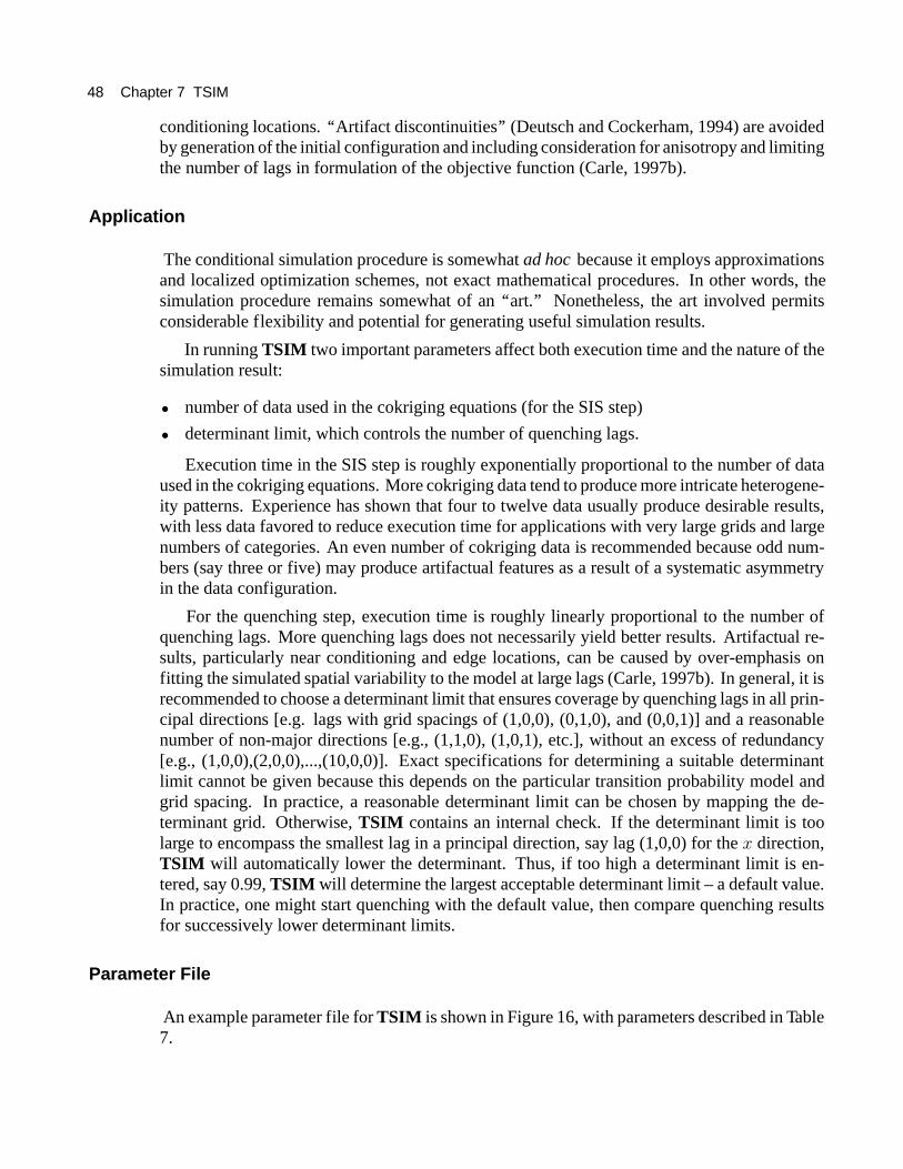
48 Chapter 7 TSIM
conditioning locations. ‘‘Artifact discontinuities’’ (Deutsch and Cockerham, 1994) are avoidedby generation of the initial configuration and including consideration for anisotropy and limitingthe number of lags in formulation of the objective function (Carle, 1997b).
Application
The conditional simulation procedure is somewhatad hocbecause it employs approximationsand localized optimization schemes, not exact mathematical procedures. In other words, thesimulation procedure remains somewhat of an ‘‘art.’’ Nonetheless, the art involved permitsconsiderable flexibility and potential for generating useful simulation results.
In runningTSIM two important parameters affect both execution time and the nature of thesimulation result:
î number of data used in the cokriging equations (for the SIS step)
î determinant limit, which controls the number of quenching lags.
Execution time in the SIS step is roughly exponentially proportional to the number of dataused in the cokriging equations. More cokriging data tend to produce more intricate heterogene-ity patterns. Experience has shown that four to twelve data usually produce desirable results,with less data favored to reduce execution time for applications with very large grids and largenumbers of categories. An even number of cokriging data is recommended because odd num-bers (say three or five) may produce artifactual features as a result of a systematic asymmetryin the data configuration.
For the quenching step, execution time is roughly linearly proportional to the number ofquenching lags. More quenching lags does not necessarily yield better results. Artifactual re-sults, particularly near conditioning and edge locations, can be caused by over-emphasis onfitting the simulated spatial variability to the model at large lags (Carle, 1997b). In general, it isrecommended to choose a determinant limit that ensures coverage by quenching lags in all prin-cipal directions [e.g. lags with grid spacings of (1,0,0), (0,1,0), and (0,0,1)] and a reasonablenumber of non-major directions [e.g., (1,1,0), (1,0,1), etc.], without an excess of redundancy[e.g., (1,0,0),(2,0,0),...,(10,0,0)]. Exact specifications for determining a suitable determinantlimit cannot be given because this depends on the particular transition probability model andgrid spacing. In practice, a reasonable determinant limit can be chosen by mapping the de-terminant grid. Otherwise,TSIM contains an internal check. If the determinant limit is toolarge to encompass the smallest lag in a principal direction, say lag (1,0,0) for the% direction,TSIM will automatically lower the determinant. Thus, if too high a determinant limit is en-tered, say 0.99,TSIM will determine the largest acceptable determinant limit – a default value.In practice, one might start quenching with the default value, then compare quenching resultsfor successively lower determinant limits.
Parameter File
An example parameter file forTSIM is shown in Figure 16, with parameters described in Table7.

Parameter File 49
4 /number of categories0.066 0.565 0.190 0.179 /proportions../llnl/sim/simxyz.bgr /output file1 /output format: 1=binary, 2=ascii1 /debugging leveltpsim.dbg /debugging file4175 /seed1 /number of simulations1966.3 -60 3. /xcenter, nx+, xsiz3023.5 -30 10.0 /ycenter, ny+, ysiz142.07 -60 0.3 /zcenter, nz+, zsiz1 4 /ndmin, ndmax1 /ibasis:0=cov,1=tp0.001 /wratio../llnl/tp/tpxyz.bgr /trans. prob. model file../llnl/tp/det.bgr /determinant file../llnl/data/llnl1195.eas /input data file-50. -50. /azimuths: coord, true1.5 1.5 /dip: coord, truejunkaz.bgr /azimuth int*1 filejunkdip.bgr /dip int*1 file 4 0.00001 -1 /maxit; tol; -1=weight,1=lag10.4 /quenching determinant limit
Figure 16. Example parameter file for TPSIM.
Line Description1 number of categories2 proportions3 output file for grid4 output format: 1=binary, 2=ASCII5 debugging level: higher yields more information6 debugging file name7 seed for random number generator8 number of simulations9 {minimum; number of nodes in{ direction;{ node size10 | minimum; number of nodes in| direction;| node size11 } minimum; number of nodes in} direction;} node size12 minimum and maximum number of data points used for cokriging estimates13 basis function for cokriging estimates: 0=covariance; 1=transition probability14 value for defining singularities in singular value decomposition (0.001 works fine)15 transition probability model file name (generated byMCMOD )16 determinant file name (generated byMCMOD )17 input data file name (GEOEAS format)18 fixed azimuths: coordinate system; stratigraphic19 fixed dips: coordinate system; stratigraphic20 specified azimuth direction file21 specified dip direction file22 quenching parameters: max# of iterations; tolerance; 1= closest lags only, -1=weight23 determinant value prescribing spatial limit of quenching lags
Table 7. Description of parameters for TPSIM.

50 Chapter 7 TSIM
Implementation Notes
î Lines 3 and 8. Line 3 constitutes the root of the output file name. If multiple realizationsare requested by setting line 8 greater than one, then an integer signifying the realizationnumber will be appended to root of the output file name. For example, if line 3 = ‘‘simu-lation.bgr’’ and line 8 = ‘‘3’’, then the output realizations will be namedsimulation.bgr1,simulation.bgr2, andsimulation.bgr3. A maximum of 100 realizations can be requested.
î Lines 9-11. The coordinate system can also be specified relative to thecenterof the simu-lated volume, rather than relative to the coordinate minima. The centered approach facilitatesmodel development in many applications because the center of a model is usually easier toestablish than the corners, particularly if the model coordinate system is rotated relative tothe data coordinate system. The centered approach can be implemented by specifyingneg-ative numbers for the number of nodes relative to the center.
Line Description9 { center;negativenumber of nodes in÷{ direction;{ node size10 | center;negativenumber of nodes in÷| direction;| node sizeentry11 } center;negativenumber of nodes in÷} direction;} node size
Thus, if ‘‘-20’’ is entered for the number of nodes in÷% direction, the number of nodes inthe%-direction of the simulation will be2û 2f n � ' e�, with % node2� centered at the ‘‘%center.’’
î Line 13. The cokriging equations are actually solved using a basis function approach(Carle, 1996). Selecting the covariance option implements simple cokriging, which willde-emphasize trends in proportions (nonstationarity of the mean) in the simulation results.
î Line 14. For more details about solving linear systems of equations with singular valuedecomposition, see Press and others (1992, p. 51-63).
î Lines 18-19. Set fixed values for coordinate system and stratigraphic azimuth and dipdirections, for example: (a) coordinate azimuth' fá, stratigraphic azimuth' fá; (b) coor-dinate azimuth' 2fá, stratigraphic azimuth' fá; (c) coordinate azimuth' fá, stratigraphicazimuth' 2fá; (d) coordinate azimuth' 2fá, stratigraphic azimuth' 2fá.
(a) (b) (c) (d)
-150 0 150-150
0
150
-150 0 150-150
0
150
-150 0 150-150
0
150
î Lines 20-21. Optional binary grid files of integer values containing localazimuth direc-tions rounded to nearest degree and localdip directions rounded to nearesttenth of a degree.If not using these options, insert bogus file names. These grids must have identical dimen-

Include File 51
sions as the simulation. This option enables generation of realizations with variable dip andstrike, as would result from structural features such as folds or geomorphic features such asmeandering or a radial pattern of deposition.
î Line 22. These are quenching parameters. No more than five quenching iterations areusually necessary – too many iterations may produce unrealistic artifacts. If the number ofiterations is set at zero, then simulated quenching will not be performed. If the number ofiterations isnegative, then simulated quenching will be performed on existing realizations asnamed by line 3. This feature is useful for examining different SIS and quenching schemes.The tolerance limit sets a criteria for terminating quenching based on the value of the ob-jective function as normalized relative to its initial value. The last parameter enables theobjective function to consider quenching lag vectors with components of no more than onenodal spacing (set' �) or to weight quenching lags by the determinant value (set' ý�).
î Redundant data. If more than one datum fall within a grid block, the simulation honorsthe first datum encountered in the data file.
Include File
The file TSIM.inc is used to dimension arrays ofTSIM . If not familiar with the dimen-sion settings, the user should checkTSIM.inc , reset dimensions (if necessary), and recompileTSIM.f(or) .
IMPORTANT! The three main 3-D arrays ofTSIM consist of integer values prescribing(a) the category at each node, (b) azimuthal direction angles rounded to nearest degree, and(c) dip direction angles rounded to nearest tenth of a degree. To conserve memory usage, diskspace, and input/output time, these arrays have been declared inTSIM.inc as 1-byte variablesinstead of the default 4-byte type. The one-byte integers may range from -128 to 127. However,the integer*1 variable type is not an ANSI FORTRAN standard, although some compilers(e.g., DEC and SGI) support it. In other cases (e.g., SUN), alogical*1 variable type canbe used to store 1-byte integer values. Therefore, the user may need to customize the variabledeclaration statement for the arrayssim , iaz , andð[ðP in TSIM.inc . One can still use thestandardinteger*4 or, alternatively, aninteger*2 declaration.
Also, because 1-byte integer or logical variables types are not standard FORTRAN, thebinary (*.bgr ) files may not transfer across different computer systems.
Output
The output fromTSIM can be produced in either ASCII or a compact binary formats.TSIMassigns negative values to any grid block with a category determined directly by conditioningdata, which facilitates highlighting and understanding of the impact of conditioning data.

8 CHUNK
CHUNK displays conditional simulations produced byTSIM in color or grayscale 3-D per-spective using the PostScript graphical language.CHUNK expects a 3-D array of integer valuesin the binary grid format, as produced byTSIM . Display of the simulation may be broken apart(exploded) into several sub-volumes (chunks), any number of which may be removed to revealinternal architecture. Grid blocks that occur on the edge of the simulation, which are prone toartifactual results, may be stripped away to reveal more representative surfaces.
Before runningCHUNK , the user must
1. Create a 3-D array of integer values in the binary grid format, such as a realization producedby TSIM .
2. Set up a parameter file.
3. Check array dimension settings inchunk.inc.
Parameter File
Figure 17 shows an example parameter file forCHUNK , with parameters described in Table8 and resulting graphical output shown in Figure 18.
Implementation Notes
î Line 4 – The option for 2, 4 or 8-bit graphics permits different numbers of possible col-ors or grayshades. The possible number of grayshades is2?Kð| where?Kð| is the numberof bits selected. Therefore, 2-bit graphics permits 4 grayshades, 4-bit graphics permits 16grayshades, and 8-bit graphics permits 256 grayshades. The possible number of colors is2Eôf?Kð|ä, which yields 64 for 2-bit, 4096 for 4-bit, and 16,777,216 for 8-bit. In general, 4-bitgraphics is more than adequate. Grayshade maps are more likely to need 8-bit graphics. Ifthe number of nodes is very large, 2-bit graphics might be useful for speeding up I/O, cuttingdown file size, or dealing with an architectural limit in PostScript mentioned below.
î Line 5 – Colorrgb (red, green, blue) values for background, axes, and title range from 0.0to 1.0. A value of 1.0 denotes full intensity. For example,rgb values are for red=(1., 0., 0.),

0 /1=landscape0.35 0.40 /x,y plot translation (inches)2.25 1.90 /x,y legend translation (inches)4 1 /nbit:2,4 or 8; color?(=1)1. 1. 1. 0. 0. 0. 0. 0. 0. /bkgr, title, axes rgb../../llnl/sim/simq.bgr /input binary grid file2 2 2 /# x,y,z chunks0. 150. 0. /x,y,z spacing betw. chunks1 /# of chunks to crop8 /chunk#’s to crop../../manual/simq.ps /output .ps file8 /# categories: cut, clr/gray-4.0 13 13 8-3.0 13 7 16-2.0 13 5 1-1.0 1 1 11.0 5 5 52.0 16 8 13.0 16 10 164.0 16 16 112 -2 -3 /shading: XY,XZ,YZ ; +=light-181.5 -305. -18.15 /Xmin,Ymin,Zmin3. 10. 0.3 /dX, dY, dZ5 5 5 5 5 5 /cropping: xl,xr,yl,yr,zl,zr150. 150. 30. /X,Y,Z scales (units/inch)150. 150. 10. /X,Y,Z label increments0 0 0 /X,Y,Z decimal places10 10 10 /X,Y,Z tics per labelStrike (m) /X titleDip (m) /Y titleVertical (m) /Z title1.00 /Data scale factor / title, line 1LLNL Aquifer System / title, line 20.95 -0.16 0.8 0.35 /concat parameters1 /legend? (1=yes)4 4 1 /# of cats; nrow,ncol1.6 2.0 /height & width5 /category #debris flow /label6 /category #floodplain /label7 /category #levee /label8 /category #channel /label
Figure 17. Example parameter file for CHUNK.
-10
Ver
tica
l (m
)
-150Strike (m)
0 150
0
150
-150
Dip (m)
010
LLNL Aquifer System
debris flow
floodplain
levee
channel
Figure 18. Example PostScript graphical output from CHUNK.
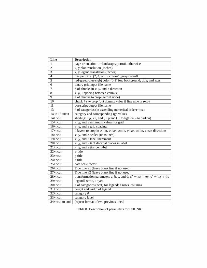
Line Description1 page orientation: 1=landscape, portrait otherwise2 x, y plot translation (inches)3 x, y legend translation (inches)4 bits per pixel (2, 4, or 8); color=1, grayscale=05 red-greed-blue (rgb) color (0-1) for: background; title; and axes6 binary grid input file name7 # of chunks in{, |, and} direction8 {> |> } spacing between chunks9 # of chunks to crop (zero if none)10 chunk #’s to crop (put dummy value if line nine is zero)11 postscript output file name13 # of categories (in ascending numerical order)=ncut14 to 13+ncut category and corresponding rgb values14+ncut shading:{|, {}, and|} plane ( + to lighten, - to darken)15+ncut {, |, and} minimum values for grid16+ncut {, |, and} grid spacing17+ncut # layers to crop in{min,{max,|min, |max,}min, }max directions18+ncut {, |, and} scales (units/inch)19+ncut {, |, and} label increment20+ncut {, |, and} # of decimal places in label21+ncut {, |, and} tics per label22+ncut { title23+ncut | title24+ncut } title25+ncut data scale factor26+ncut Title line #1 (leave blank line if not used)27+ncut Title line #2 (leave blank line if not used)28+ncut transformation parameters a, b, c, and d:{3 @ d{. f|; |3 @ e{. g|29+ncut legend? 0=no, 1=yes30+ncut # of categories (ncat) for legend; # rows, columns31+ncut height and width of legend32+ncut category #33+ncut category label34+ncut to end (repeat format of two previous lines)
Table 8. Description of parameters for CHUNK.

Include File 55
green=(0.,1.,0.), blue=(0.,0.,1.), yellow=(1.,1.,0.), cyan=(0.,1.,1.), and magenta=(1.,0.,1.).Grayshades can be produced by setting allrgb intensities equal with (0.,0.,0.)=black and(1.,1.,1.)=white.
î Line 10 - Numbering of chunks is based on order in which they are drawn, from lower backleft to upper front right, cycling byn%,ý+, andn5.
î Lines 14 to 13+ncut– Grayshade andrgb intensities are specified by integer values of(1,2,3,4) for 2-bit graphics, (1,2,3,...,16) for 4-bit graphics, and (1,2,3,...,256) for 8-bit graph-ics. These values are then scaled to intensities ranging from 0.0 and 1.0. If a grayshade imageis requested (second parameter in line 4 set to zero), only one value per line is needed (versusthree per line for color).
î Line 17+ncut - Use these settings to crop off layers on the outer edges of a realization. Edgeeffects may mask more representative surfaces underneath.
î Line 28+ncut – The@, M, U, and_ transformation parameters used to create the quasi 3-D perspective should maintain@2 n U2 é � andM2 n _2 é � to preserve%c +c 5 scalingrelationships.
î Architectural Limit – Note that Postscript contains an architectural limit of 65535 elementsin any array or string. What this means forCHUNK is that garbled results will occur on anyface of a chunk that utilizes more than 262140 bits. One can get around this limitation bydividing the image into more chunks and/or using less bits per pixel.
Include File
The file chunk.inc is used to dimension arrays ofCHUNK . The main array setting controlsthe size of the grid that can be visualized. If not familiar with the dimension settings, the usershould checkchunk.inc, reset dimensions (if necessary), and recompilechunk.f(or).
IMPORTANT! CHUNK reads in the 3-D simulation array produced byTSIM . Recall thatthe variable type for the simulation array was set inTSIM.inc , so the corresponding variabletype for the 3-D array specified inchunk.inc and read intoCHUNK must be the same! There-fore, whether your system acceptsinteger*1 , logical*1 , or whatever, just make surethat both thesim array inTSIM.inc and theival1 array inchunk.inc are declared as thesame variable type.

9 PostScript Basics
Regular PostScript (*.ps) Files
The output files fromGRAFXX andCHUNK are produced in the PostScript (PS) graphicallanguage. Inevitably, the user will need or want to modify the graphical output. In many cases,modifications can be made quite simply by editing the ASCII format PS file (*.ps). Some basicproperties which are useful for editing PS files are:
î All text strings are surrounded by parentheses. One can modify the text string by searchingfor (finding) it, then modifying the text string within the parentheses.
î On a line previous to a text string, a command such as234.00 489.00 m designates theX,Y page coordinates of the text string in 72nds of an inch. One can modify the coordinatesto move the location of the text string.
î A command such as72 144 translate will translate subsequent graphics in the fileby the X,Y page units specified.
î A command such as2.0 2.0 scale will scale subsequent graphics by factors of 2.0 inthe X and Y page directions.
î The commandsfindfont , scalefont , andsetfont find, scale, andset the currentfont.
Further details can be found in many reference texts such as the PostScript Language Ref-erence Manual (Adobe Systems Incorporated, 1990).
Encapsulated PostScript (*.eps) Files
Although regular PS files can be directly interpreted by printers and on-screen viewers, theyusually are not readily incorporated into word processing or slide presentation programs. TheEncapsulated PostScript (EPS) format, however, is quite portable. The regular PS files (*.ps)produced byGRAFXX andCHUNK can be converted to EPS files (*.eps) by adding necessaryheader and footer information. This information can be added using the programps2eps.f(or).
BoundingBox
The most important of the added EPS information is a ‘‘BoundingBox,’’ which specifies thelower left andupper right X,Y corner coordinates of the plot in units of 1/72 of an inch. TheBoundingBox provides an opportunity to crop unneeded blank space surrounding the plot.

57
simq.ps /postscript input filesimq.eps /encapsulated postscript file77 251 548 583 /bounding box (in inches)Steve Carle /creator9/9/97 /date3:00PM /time
Figure 19. Example parameter file for PS2EPS.
An obvious way to define a suitable BoundingBox is to print out the PS file, then measurethe displacements of the desired lower left and upper right corners relative to the lower leftcorner of the page.
An easier way to define a BoundingBox is to employ the Ghostview previewer, whichdisplays PS or EPS files on screen. In the upper left corner, Ghostview tracks plot coordinatesin units of 1/72 of an inch whenever the Mouse-driven crosshairs are located on the screen viewof the plot. Thus, one can find suitable BoundingBox coordinates by moving the crosshairs tothe desired lower left and upper right corners.
PS2EPS
Theps2eps.f(or)program is implemented in the same manner as all other T-PROGS programs.An example parameter file is shown in Figure 19, with parameters described in Table 9.
Line Description1 input PostScript file name2 output Encapsulated PostScript file name3 BoundingBox in 72nds of an inch: lower left X,Y; upper right X,Y4 name of plot creator5 date6 time
Table 9. Description of parameters for PS2EPS.
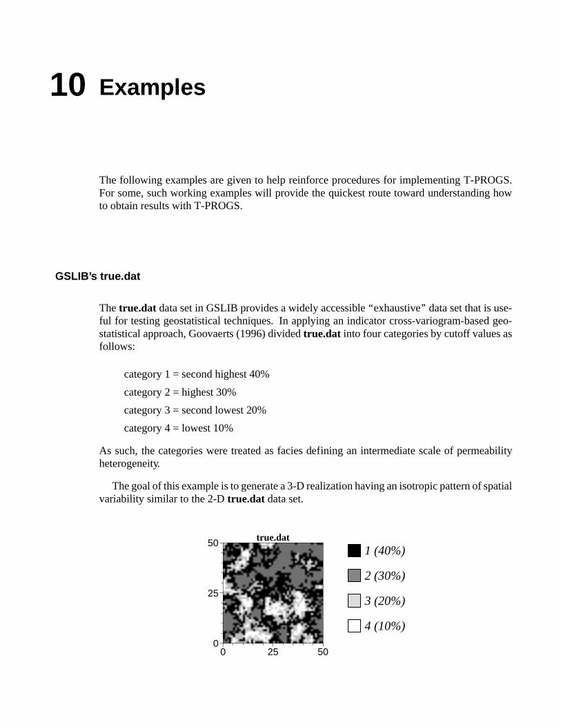
10 Examples
The following examples are given to help reinforce procedures for implementing T-PROGS.For some, such working examples will provide the quickest route toward understanding howto obtain results with T-PROGS.
GSLIB’s true.dat
Thetrue.dat data set in GSLIB provides a widely accessible ‘‘exhaustive’’ data set that is use-ful for testing geostatistical techniques. In applying an indicator cross-variogram-based geo-statistical approach, Goovaerts (1996) dividedtrue.dat into four categories by cutoff values asfollows:
category 1 = second highest 40%
category 2 = highest 30%
category 3 = second lowest 20%
category 4 = lowest 10%
As such, the categories were treated as facies defining an intermediate scale of permeabilityheterogeneity.
The goal of this example is to generate a 3-D realization having an isotropic pattern of spatialvariability similar to the 2-Dtrue.dat data set.
true.dat
0 25 500
25
501 (40%)
2 (30%)
3 (20%)
4 (10%)

GSLIB’s true.dat 59
Step 1 – Put data into GEOEAS format
true.dat categorized by 0.15 0.44 and 2.12 cutoffs 7 x y z 1=2nd highest 40% 2=highest 30% 3=2nd lowest 20% 4=lowest 10% 1.00000 1.00000 0. 0 1 0 0 2.00000 1.00000 0. 0 1 0 0 3.00000 1.00000 0. 0 1 0 0 4.00000 1.00000 0. 1 0 0 0 5.00000 1.00000 0. 0 0 0 1 6.00000 1.00000 0. 0 0 0 1 7.00000 1.00000 0. 0 0 1 0 8.00000 1.00000 0. 0 0 1 0 9.00000 1.00000 0. 0 0 1 0 10.00000 1.00000 0. 0 0 1 0 11.0000 1.00000 0. 0 0 1 0 12.0000 1.00000 0. 0 0 1 0...etc.
Step 2 – Calculate isotropic transition probabilities using GAMEAS
It is assumed that the pattern of spatial variability is isotropic and, thus, does not depend on di-rection. The omni-directional statistics are computed by employing a large azimuth bandwidthand an azimuth angle tolerance of slightly greater than 90á.
START OF PARAMETERS../true/truecat.eas /input file1 2 3 /x,y,z columns4 4 5 6 7 /nvar, var1,2,3,... columns-1. 2. /vmin, vmax../true/tp.eas /output file25 /# lags1. /lag spacing0.5 /lag tolerance1 /ndir0.2 90.1 10000000. 0.0 22.50 0.25 /az,daz,azbw;dip,ddip,dipbw16 /# of bivariate statistics1 1 11 /j,k, 11=tp1 2 111 3 111 4 112 1 112 2 112 3 112 4 113 1 113 2 113 3 113 4 114 1 114 2 114 3 114 4 11
Step 3 – Plot the transition probability data matrix using GRAFXX
Plot the transition probability data before proceeding to modeling spatial variability. The qualityof the data will influence the choice of modeling approach.

60 Chapter 10 Examples
0 /symmetry check (1=sym)0.20 0.20 /dx dy between plots (inches)0 /line at zero? 1=yes1 /number of input files../../true/tp.eas /input file 1-10 0.40 0 1.00 /file 1: marker, lw, dash, gray../../true/tp.ps /output file4 /number of categories0. 20. -0.1 1.0 /Xmin,Xmax,Ymin,Ymax0 1 /# of X,Y decimal places15. 0.825 /X,Y scales (units/inch)1.0 /Data scale factor0.0 /axes gray level5. 0.5 /X,Y label increments5 5 /X,Y tics per labelLag (grid units) /X title /Y title0 /1= titles for each plot1 /X title variable 11 /Y title variable 12 /X title variable 22 /Y title variable 23 /X title variable 33 /Y title variable 34 /X title variable 44 /Y title variable 4 /title, line 1Transition Probability /title, line 21 /1=plot legend6.5 /width of legend (inches)Measured /name of variable 1
Lag (grid units)
12
3
1
4
0 5 10 15 20
0.0
0.5
1.0
2 3 4
Transition Probability
Measured
Step 4 – Model spatial variability using MCMOD
In this example, option 2 is initially employed using transition probability data for the secondlag ({û ' 2é2) to model spatial variability in all principal directions.
4 /# of categories0.4016 0.3004 0.2008 0.0972 /proportions2 /background category../true/mcmod.dbg /name of debugging file../true/tpxy2.bgr /output file for 3-D model../true/det2.bgr /output file for determinant0.002 0.002 0.002 /determinant extent for 3-D model1. 1. 1. /dhx,dhy,dhz for 3-D model../true/tpxm2.eas /X-direction output file201 0.10 /X-Direction: # lags, spacing2 /1=r,2=d,3=etp,4=etf,5=i,6=p,7=f../true/tp.eas /data file2 /lag../true/tpym2.eas /Y-direction output file100 0.25 /Y-Direction; # lags, spacing2 /1=r,2=d,3=etp,4=etf,5=i,6=p,7=f../true/tp.eas /data file2 /lag../true/tpzm2.eas /Z-direction output file100 0.25 /Z-Direction: # lags, spacing2 /1=r,2=d,3=etp,4=etf,5=i,6=p,7=f../true/tp.eas /data file2 /lag

GSLIB’s true.dat 61
Step 5 – Examine debugging output from MCMOD
Warnings are given that several off-diagonal entries have negative transition rates (Don’t panic!).Clearly, this categorization oftrue.dat data set yields very strong juxtapositional tendencies of2 $ � $ ô $ e $ ô $ � $ 2. The negative transition rates are caused by very hightransition probabilities for�? 2 andô? e at the second lag ({û ' 2é2).
The debugging output contains useful interpretive information. Juxtapositional tendenciesappear fairly symmetric, because opposing off-diagonal entries of embedded transitionfrequen-ciesare similar in magnitude. The symmetry is also evident in the coefficients of the transitionrates with respect to independent transition frequencies, which also indicate the strong jux-tapositional tendencies between� ? 2 andô ? e by coefficients much greater than unity.Transition rates of zero or less indicate that the categories are rarely, if ever, juxtaposed next toeach other.
At the bottom of the debugging file, the lateral extent of the 3-D model is given in incrementsof nodal spacing. Make sure the lateral extent is large (or small) enough to encompass ranges ofcorrelation for most or all of the categories. Recall that reducing the determinant limit increasesthe lateral extent of the 3-D model.
MCMOD debugging file Parameter file: mcmod.parNumber of categories: 4Proportions: 0.4016 0.3004 0.2008 0.0972Background category: 2 ------- X-DIRECTION: -------Method - option 2: trans. prob. at specified lag1-D model output file: ../goofball/tpxm2.easWARNING: Off-diagonal Transition Rate 1 2 is too large for columnWARNING: Off-diagonal Transition Rate 1 4 is negative.WARNING: Off-diagonal Transition Rate 2 1 is too large for row 2WARNING: Off-diagonal Transition Rate 2 3 is negative.WARNING: Off-diagonal Transition Rate 3 2 is negative.WARNING: Off-diagonal Transition Rate 3 4 is too large for columnWARNING: Off-diagonal Transition Rate 4 1 is negative.WARNING: Off-diagonal Transition Rate 4 3 is too large for row 4 Rate Matrix for X-Direction: -0.552953 0.251718 0.330448 -0.029212 0.339745 -0.285394 -0.063882 0.009531 0.653765 -0.086431 -0.972821 0.405488 -0.115940 0.020553 0.841820 -0.746433 embedded transition probabilities: 1.000000 0.455224 0.597606 -0.052830 1.190444 1.000000 -0.223839 0.033395 0.672030 -0.088846 1.000000 0.416816 -0.155326 0.027535 1.127791 1.000000 embedded transition frequencies: 0.385736 0.175596 0.230518 -0.020378 0.177281 0.148920 -0.033334 0.004973 0.228031 -0.030147 0.339317 0.141433 -0.019575 0.003470 0.142133 0.126027 entropy= -1032.46 w.r.t. independent transition freqs:( 1.8085) 2.2039 0.9605 -0.3085 2.2250 ( 3.5039) -0.6139 0.3327 0.9501 -0.5552 ( 1.0279) 3.1416 -0.2963 0.2322 3.1571 ( 1.3397) w.r.t. volumetric proportions:( 1.8085) 0.9068 1.7809 -0.3252 2.0738 ( 3.5039) -0.7799 0.2404 1.3374 -0.2364 ( 1.0279) 3.4272 -0.3492 0.0828 5.0706 ( 1.3397) w.r.t. # of embedded occurrences( 1.8085) 1.8777 1.0818 -0.2575 2.6266 ( 3.5039) -0.5614 0.2255 1.1510 -0.3942 ( 1.0279) 2.1851 -0.3519 0.1616 2.9048 ( 1.3397)... Constructing 3-D transition probability model # of lags in +x,+y,+z direction = 7 8 8 total # of lags = 4335
Step 6 – Compare measured and modeled transition probabilities
The comparison is accomplished by slight modifications to theGRAFXX parameter file usedin step 3.
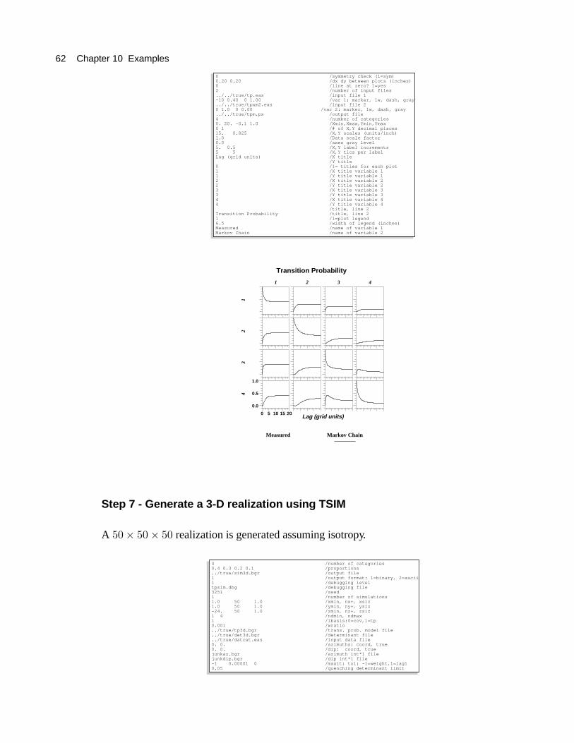
62 Chapter 10 Examples
0 /symmetry check (1=sym)0.20 0.20 /dx dy between plots (inches)0 /line at zero? 1=yes2 /number of input files../../true/tp.eas /input file 1-10 0.40 0 1.00 /var 1: marker, lw, dash, gray../../true/tpxm2.eas /input file 20 1.0 0 0.00 /var 2: marker, lw, dash, gray../../true/tpm.ps /output file4 /number of categories0. 20. -0.1 1.0 /Xmin,Xmax,Ymin,Ymax0 1 /# of X,Y decimal places15. 0.825 /X,Y scales (units/inch)1.0 /Data scale factor0.0 /axes gray level5. 0.5 /X,Y label increments5 5 /X,Y tics per labelLag (grid units) /X title /Y title0 /1= titles for each plot1 /X title variable 11 /Y title variable 12 /X title variable 22 /Y title variable 23 /X title variable 33 /Y title variable 34 /X title variable 44 /Y title variable 4 /title, line 2Transition Probability /title, line 21 /1=plot legend6.5 /width of legend (inches)Measured /name of variable 1Markov Chain /name of variable 2
Lag (grid units)
12
3
1
4
0 5 10 15 20
0.0
0.5
1.0
2 3 4
Transition Probability
Measured Markov Chain
Step 7 - Generate a 3-D realization using TSIM
A Dfû Dfû Df realization is generated assuming isotropy.
4 /number of categories0.4 0.3 0.2 0.1 /proportions../true/sim3d.bgr /output file1 /output format: 1=binary, 2=ascii1 /debugging leveltpsim.dbg /debugging file3251 /seed1 /number of simulations1.0 50 1.0 /xmin, nx+, xsiz1.0 50 1.0 /ymin, ny+, ysiz-24. 50 1.0 /zmin, nz+, zsiz1 4 /ndmin, ndmax1 /ibasis:0=cov,1=tp0.001 /wratio../true/tp3d.bgr /trans. prob. model file../true/det3d.bgr /determinant file../true/datcat.eas /input data file0. 0. /azimuths: coord, true0. 0. /dip: coord, truejunkaz.bgr /azimuth int*1 filejunkdip.bgr /dip int*1 file-1 0.00001 0 /maxit; tol; -1=weight,1=lag10.05 /quenching determinant limit

GSLIB’s true.dat 63
Step 8 - View realization using CHUNK
0 0 /1=landscape; 1=11x17-0.5 0. /x,y plot translation (inches)3.50 2.50 /x,y legend translation (inches)4 0 /nbit 2,4,8; color(1) or gray(0)1. 1. 1. 0. 0. 0. 0. 0. 0. /bkgr, title, axes rgb../../true/sim3d.bgr /input binary grid file1 1 2 /# x,y,z chunks0. 0. 40. /X,Y,Z spacing betw. chunks0 /# of chunks to crop1 /chunk#’s to crop../../true/true3d.ps /output .ps file-128. 127. /gmin gmax8 /# cutoffs: cut, clr/gray-4.0 16-3.0 13-2.0 8-1.0 1 1.0 1 2.0 8 3.0 13 4.0 161 -2 -1 /shading: XY,XZ,YZ ; +=light0. 0. -24.5 /Xmin,Ymin,Zmin1. 1. 1. /dX, dY, dZ0 0 0 0 0 0 /cropping: xl,xr,yl,yr,zl,zr20. 20. 20. /X,Y,Z scales (units/inch)20. 20. 20. /X,Y,Z label increments0 0 0 /X,Y,Z decimal places5 5 5 /X,Y,Z tics per labelx (ft) /X titley (ft) /Y titlez (ft) /Z title1.00 /Data scale factor3-D conditional simulation / title, line 1based on "true.dat" data set / title, line 20.92 -0.4 0.7 0.48 /concat parameters2 0 /legend? (0=no), vert?4 4 1 /# of cats; nrow,ncol2.0 2.0 /height & width5 /category 11 (40%) /label6 /category 22 (30%) /label7 /category 33 (20%) /label8 /category 44 (10%) /label
-20
0
z (f
t)
0
2040x (ft)
0
20
40
y (ft)
20
3-D conditional simulationbased on "true.dat" data set

64 Chapter 10 Examples
LLNL Data Set
The Lawrence Livermore National Laboratory (LLNL) data set consists of about 5,500 m ofsemi-continuous vertical profiles (logs) of core descriptions of alluvial sediments obtained from125 boreholes drilled for hydrogeologic characterization of the shallow aquifer system under-lying LLNL (Qualheim, 1988). Lithofacies were categorized asdebris flow(poorly sorted clay,silt, sand, gravel),floodplain (clay and silt),levee(silty fine sand), andchannel (moderatelyto well sorted sand and gravel) deposits. This categorization was based on geologic interpre-tation of the depositional system with consideration for contrasts in hydrogeologic properties,to serve as a geologically sound basis for defining ‘‘hydrofacies’’ in detailed 3-D models of thegroundwater flow system (Noyes, 1990).
Step 1 – Put data into GEOEAS format
Data 7 x = easting y = northing z = elevation above mean sea level 1 = debris flow 2 = floodplain 3 = levee 4 = channel 2132.8 2487.4 137.07 0 1 0 0 2132.8 2487.4 136.77 0 1 0 0 2132.8 2487.4 136.47 0 1 0 0 2132.8 2487.4 136.17 0 1 0 0 2132.8 2487.4 135.87 1 0 0 0 2132.8 2487.4 135.57 1 0 0 0 2132.8 2487.4 132.27 0 1 0 0 2132.8 2487.4 131.97 0 1 0 0 2576.2 2695.5 186.48 0 1 0 0 2576.2 2695.5 182.28 0 0 0 1 2576.2 2695.5 181.98 0 0 0 1 2576.2 2695.5 181.68 0 0 0 1 2576.2 2695.5 181.38 0 0 0 1 2576.2 2695.5 181.08 0 1 0 0 2576.2 2695.5 175.98 1 0 0 0 2576.2 2695.5 175.68 0 1 0 0 2576.2 2695.5 175.38 0 1 0 0 2576.2 2695.5 112.98 0 1 0 0...
Step 2 – Calculate vertical transition probabilities using GAMEAS
START OF PARAMETERSdata.eas /input file1 2 3 /x,y,z columns4 4 5 6 7 /nvar, var1,2,3,... columns-1. 2. /vmin, vmaxdatatpz.eas /output file41 /# lags0.3000 /lag spacing0.1500 /lag tolerance1 /ndir0.0 90. 0.25 -90.0 22.50 0.25 /az,daz,azbw;dip,..,..16 /# of bivariate statistics1 1 11 /j,k, 11=tp1 2 111 3 111 4 112 1 112 2 112 3 112 4 113 1 113 2 113 3 113 4 114 1 114 2 114 3 114 4 11

LLNL Data Set 65
Step 3 – Plot vertical transition probabilities using GRAFXX
0 /symmetry check (1=sym)0.20 0.20 /dx dy between plots (inches)0 /line at zero? 1=yes1 /number of input files../../llnl/tp/llnl1195tpz.eas /input file 1-10 0.55 0 1. /file 1: marker, lw, dash, gray../../manual/llnl/llnltpz.ps /output file4 /number of categories0. 6. 0.0 1.0 /Xmin,Xmax,Ymin,Ymax0 1 /# of x,y decimal places5.4 0.9 /X,Y scales (units/inch)1.0 /Data scale factor0. 0. 0. /axes color3. 0.5 /X,Y label increments3 5 /X,Y tics per labelLag (m) /X title /Y title0 /1= titles for each plotdebris fl /X title variable 1debris fl /Y title variable 1floodplain /X title variable 2floodplain /Y title variable 2levee /X title variable 3levee /Y title variable 3channel /X title variable 4channel /Y title variable 4 /title, line 1Transition Probability - Vertical /title, line 21 /1=plot legend7.5 /width of legend (inches)Measured /label for file 1 data
Lag (m)
debr
is f
lfl
oodp
lain
leve
e
debris fl
chan
nel
0 3 60.0
0.5
1.0
floodplain levee channel
Transition Probability - Vertical
Measured
Step 4 – Calculate lateral transition probabilities using GAMEAS
Although the alluvial fan facies architecture is expected to be highly anisotropic, the lateraltransition probabilities were calculated as if lateral isotropy were assumed. The anisotropydirections in the LLNL alluvial system substantially vary because of radial fan morphology,variation in fan source location, fan commingling, fluvial meandering, and deformation. Theisotropic calculation was made under the assumption that the resulting transition probabilitieswould primarily reflect an upper limit to the strike-direction spatial continuity. It would alsoprescribe a lower limit to the dip-direction spatial continuity.
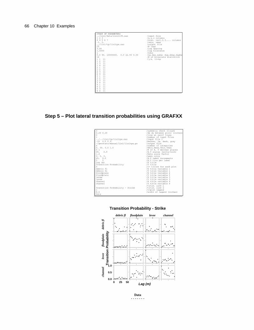
66 Chapter 10 Examples
START OF PARAMETERS../llnl/data/llnl1195.eas /input file1 2 3 /x,y,z columns4 4 5 6 7 /nvar, var1,2,3,... columns-1. 2. /vmin, vmax../llnl/tp/llnltpx.eas /output file25 /# lags3.00 /lag spacing1.5000 /lag tolerance1 /ndir0.0 90. 10000000. 0.0 22.50 0.30 /az,daz,azbw; dip,ddip,dipbw16 /# of bivariate statistics1 1 11 /j,k, 11=tp1 2 111 3 111 4 112 1 112 2 112 3 112 4 113 1 113 2 113 3 113 4 114 1 114 2 114 3 114 4 11
Step 5 – Plot lateral transition probabilities using GRAFXX
0 /symmetry check (1=sym)0.20 0.20 /dx dy between plots (inches)0 /line at zero? 1=yes1 /number of input files../../llnl/tp/llnltpx.eas /input file 1-10 0.5 0 0. /marker, lw, dash, gray~/geostats/manual/llnl/llnltpx.ps /output file4 /number of categories0. 50. 0.0 1.0 /Xmin,Xmax,Ymin,Ymax0 1 /# of X, Y decimal places45. 0.9 /X,Y scales (units/inch)1.0 /Data scale factor0. 0. 0. /axes color25. 0.5 /X,Y label increments5 5 /X,Y tics per labelLag (m) /X titleTransition Probability /Y title0 /1= titles for each plotdebris fl /X title variable 1debris fl /Y title variable 1floodplain /X title variable 2floodplain /Y title variable 2levee /X title variable 3levee /Y title variable 3channel /X title variable 4channel /Y title variable 4 /title, line 1Transition Probability - Strike /title, line 21 /1=plot legend8.5 /width of legend (inches)Data
Lag (m)
Tra
nsi
tio
n P
rob
abili
tyde
bris
fl
floo
dpla
inle
vee
debris fl
chan
nel
0 25 500.0
0.5
1.0
floodplain levee channel
Transition Probability - Strike
Data

LLNL Data Set 67
Step 6 – Develop 1- and 3-D Markov Chain models using MCMOD
The following procedure, used to develop the LLNL principal direction models, may guideapplication ofMCMOD to typical data sets derived from boreholes:
1. Initially develop the vertical-direction model, using either option 1, 2, or 3. For the strike anddip directions, arrive at plausible mean lengths consistent with the transition probability data(if available) to define the diagonal entries. For the off-diagonal entries, assume symmetryand use option 3 to estimate embedded transition probabilities. By assuming symmetryand a background category, only three of the twelve off-diagonal transition rates need to beprescribed for a four-category system (only one of six for a three-category system).
2. Look at the debugging output file fromMCMOD , which includes other interpretations yield-ing an equivalent Markov chain model. Option 3, the embedded transition probability frame-work, is usually the most interpretable. If necessary, refine the vertical-direction model.
3. For the strike and dip-direction models, initiate the off-diagonal embedded transition proba-bilities by considering Walther’s Law concepts, that vertical facies successions reflect lateralfacies successions. For the off-diagonal terms needed to complete the strike and dip direc-tion models, assign the embedded transition probabilities obtained from the vertical model.Refine the strike and dip direction models as necessary to maintain geologic plausibility,adherence to probability law, and consistency with transition probability data.
4 /# of categories0.066 0.565 0.190 0.179 /proportions2 /background category../llnl/tp/mcmod.dbg /name of debugging file../llnl/tp/tpxyz.bgr /output file for 3-D model../llnl/tp/det.bgr /output file for determinant0.05 0.05 0.05 /determinant limits for 3-D model3.0 10.0 0.30 /dhx,dhy,dhz for 3-D model../llnl/tp/llnltpxm.eas /X-direction output file200 1. /X-Direction: # lags, spacing3 /option: 1=r,2=d,3=etp,4=etf,5=i8.0 0. -1. -1.0. 0. 0. 0.0.027 0. 6.0 -1.0.041 0. 0.839 10.../llnl/tp/llnltpym.eas /Y-direction output file200 2.5 /Y-Direction; # lags, spacing3 /1=r,2=d,3=etp,4=etf,5=i,6=p,7=f24. 0. -1. -1. 0. 0. 0. 0. 0.027 0. 20.0 -1. 0.041 0. 0.839 50.../llnl/tp/llnltpzm3.eas /Z-direction output file200 0.1 /Z-Direction: # lags, spacing2 /option: 1=r,2=d,3=etp,4=etf,5=i../llnl/tp/llnl1195tpz.eas /data file3 /lag #
MCMOD debugging file Parameter file: mcmodllnl3.parNumber of categories: 4Proportions: 0.0660 0.5650 0.1900 0.1790Background category: 2 ------- X-DIRECTION: -------...------- Z-DIRECTION: -------Method - option 2: trans. prob. at specified lag1-D model output file: ../llnl/tp/llnltpzm3.easWARNING: Off-diagonal Transition Rate 4 2 is negative. Rate Matrix for Z-Direction: -0.871510 0.702561 0.103207 0.065742 0.079481 -0.435999 0.150644 0.205875 0.029521 1.073549 -1.227927 0.124857 0.039128 -0.022367 0.789836 -0.806597 embedded transition probabilities: 1.000000 0.806142 0.118423 0.075434 0.182296 1.000000 0.345514 0.472190 0.024042 0.874278 1.000000 0.101681 0.048510 -0.027731 0.979221 1.000000 embedded transition frequencies: 0.084396 0.068035 0.009994 0.006366 0.065889 0.361442 0.124883 0.170669 0.008230 0.299282 0.342319 0.034807 0.010276 -0.005875 0.207441 0.211843 entropy= -56.8526 w.r.t. independent transition freqs:( 1.1474) 1.8393 0.3121 0.4138 1.7813 ( 2.2936) 0.5699 1.6207 0.2570 1.3657 ( 0.8144) 0.3819 0.6679 -0.0558 2.2758 ( 1.2398)... Constructing 3-D transition probability model # of lags in +x,+y,+z direction = 7 7 9 total # of lags = 4275

68 Chapter 10 Examples
Step 7 – Calculate independent or maximum entropy (disorder) model
4 /# of categories0.066 0.565 0.190 0.179 /proportions2 /background category../llnl/tp/mcmodtpze.dbg /name of debugging file../llnl/tp/tpxyze.bgr /output file for 3-D model../llnl/tp/dete.bgr /output file for determinant1.000 1.000 1.000 /determinant limit for 3-D model3.0 10.0 0.30 /dhx,dhy,dhz for 3-D model../llnl/tp/llnltpxme.eas /X-direction output file200 1. /X-Direction: # lags, spacing5 /option: 1=r,2=d,3=etp,4=etf,5=i8.0 0. 1. 1.0. 22.965 0. 0.1.0 0. 6.0 1.1.0 0. 1.0 10.../llnl/tp/llnltpyme.eas /Y-direction output file200 2.5 /Y-Direction; # lags, spacing5 /option: 1=r,2=d,3=etp,4=etf,5=i24. 0. 1. 1. 0. 62.665 0. 0. 1.0 0. 20.0 1. 1.0 1. 1. 50.../llnl/tp/llnltpzme3.eas /Z-direction output file200 0.1 /Z-Direction: # lags, spacing5 /option: 1=r,2=d,3=etp,4=etf,5=i1.1474 0. 1. 1.0. 2.2936 0. 0.1.0 0. 0.8144 1.1.0 0. 1. 1.2398
Step 8 – Compare measured and modeled transition probabilities
0 /symmetry check (1=sym)0.20 0.20 /dx dy between plots (inches)0 /line at zero? 1=yes5 /number of input files../../llnl/tp/llnltpx.eas /input file 1-10 0.5 0 0. /marker, lw, dash, gray../../llnl/tp/llnltpxm.eas /input file 50 1.0 0 0. /marker, lw, dash, gray../../llnl/tp/proptpx.eas /input file 20 0.5 1 0. /marker, lw, dash, gray../../llnl/tp/mltpx.eas /input file 30 0.5 3 0. /marker, lw, dash, gray../../llnl/tp/llnltpxme.eas /input file 40 1.0 0 0.8 /marker, lw, dash, gray~/geostats/manual/llnl/llnltpxm.ps /output file4 /number of categories0. 50. 0.0 1.0 /Xmin,Xmax,Ymin,Ymax0 1 /# of X, Y decimal places45. 0.9 /X,Y scales (units/inch)1.0 /Data scale factor0. 0. 0. /axes color25. 0.5 /X,Y label increments5 5 /X,Y tics per labelLag (m) /X titleTransition Probability /Y title0 /1= titles for each plotdebris fl /X title variable 1debris fl /Y title variable 1floodplain /X title variable 2floodplain /Y title variable 2levee /X title variable 3levee /Y title variable 3channel /X title variable 4channel /Y title variable 4 /title, line 1Transition Probability - Strike /title, line 21 /1=plot legend7.5 /width of legend (inches)DataModelProp.LengthDisorder

LLNL Data Set 69
Lag (m)
Tra
nsi
tio
n P
rob
abili
tyde
bris
fl
floo
dpla
inle
vee
debris fl
chan
nel
0 25 500.0
0.5
1.0
floodplain levee channel
Transition Probability - Strike
Data Model Prop. Length Disorder
Step 9 – Generate a 3-D realization using TSIM
4 /number of categories0.07 0.56 0.19 0.18 /proportions../examples/llnlsim.bgr /output file1 /debugging leveltpsim.dbg /debugging file2311 /seed1 /number of simulations1955.292 -200 3.0 /xcenter, nx, xsiz2692.908 -100 10.0 /ycenter, ny, ysiz 127.50 -241 0.3 /zcenter, nz, zsiz1 4 /ndmin, ndmax1 /ibasis:0=cov,1=tp0.001 /wratio../tp/llnltpxyz.bgr /trans. prob. model file../tp/llnldetxyz.bgr /spectral radius file../data/llnl1195.eas /input data file0. 0. /azimuths: coord, true0. 0. /dip: coord, true../examples/llnlaz.bgr /azimuth int*1 file../examples/llnldip.bgr /dip int*1 file4 0.00001 0 /maXit; tol; -1=no dcl,1=lag10.5 /quenching determinant limit

70 Chapter 10 Examples
Step 10 – View realization using CHUNK
1 /landscape(1) or portrait(0)3.0 3.5 /x y plot translation3.5 10.0 /x y legend translation4 0 /nbit 2,4,8; color(1)or gray(0)1. 1. 1. 0. 0. 0. 0. 0. 0. /rgb: bkgr, title, axes../examples/llnlsim.bgr /input binary grid file2 2 2 /# x,y,z chunks330. 0. 110. /X,Y,Z spacing betw. chunks1 /# of chunks to crop8 /chunk #’s to crop../examples/llnlsim.ps /output .ps file10 /# of categories-128. 5 /value, gray-4.0 1-3.0 13-2.0 16-1.0 81.0 82.0 163.0 134.0 1127. 140 -2 -1 /shading: XY,XZ,YZ(+light -dark)-601.5 -1005. 55.05 /Xmin,Ymin,Zmin3. 10. 0.3 /dX, dY, dZ33 33 40 40 5 83 /cropping: xl,xu,yl,yu,zl,zu160. 160. 32. /X,Y,Z scales (units/inch)250. 250. 20. /X,Y,Z label increments0 0 0 /X,Y,Z decimal places5 5 4 /X,Y,Z tics per labelNortheast (m) /X titleNorthwest (m) /Y titleElevation (m) /Z title1.00 /Data scale factor / title, line 2 / title, line 2.707 -.707 0.95 0.312 /concat paramters2 0 0 /legend, legend orientation?4 4 1 /# of categories; #rows,cols1.6 1.0 /legend height, width6 /category #debris flow /label7 /category #floodplain /label8 /category #levee /label9 /category #channel /label
60
80
100
Elevation (m)
-500
-250
0
Northeast (m)0
250
500
0
250
500
-500
-250
0
Northwest (m)
120
140
160
debris flow
floodplain
levee
channel
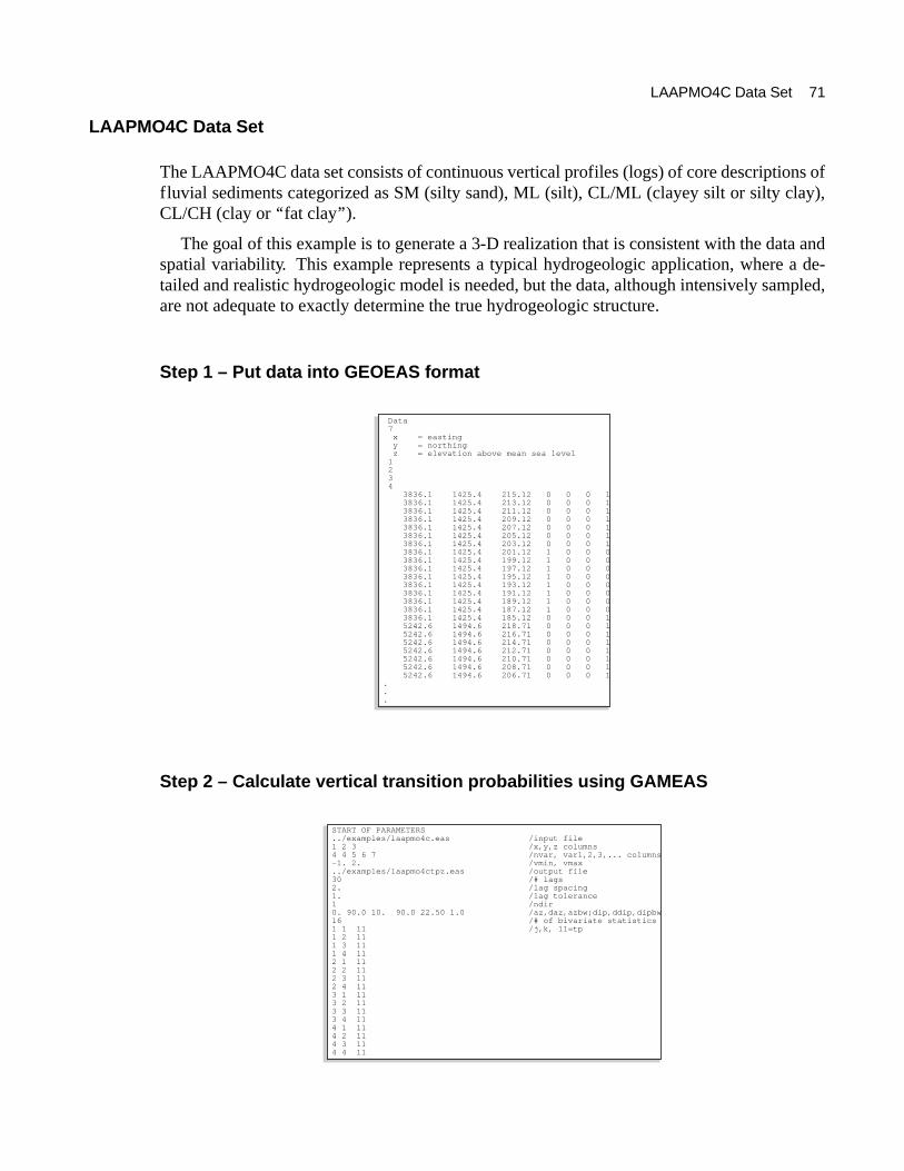
LAAPMO4C Data Set 71
LAAPMO4C Data Set
The LAAPMO4C data set consists of continuous vertical profiles (logs) of core descriptions offluvial sediments categorized as SM (silty sand), ML (silt), CL/ML (clayey silt or silty clay),CL/CH (clay or ‘‘fat clay’’).
The goal of this example is to generate a 3-D realization that is consistent with the data andspatial variability. This example represents a typical hydrogeologic application, where a de-tailed and realistic hydrogeologic model is needed, but the data, although intensively sampled,are not adequate to exactly determine the true hydrogeologic structure.
Step 1 – Put data into GEOEAS format
Data 7 x = easting y = northing z = elevation above mean sea level 1 2 3 4 3836.1 1425.4 215.12 0 0 0 1 3836.1 1425.4 213.12 0 0 0 1 3836.1 1425.4 211.12 0 0 0 1 3836.1 1425.4 209.12 0 0 0 1 3836.1 1425.4 207.12 0 0 0 1 3836.1 1425.4 205.12 0 0 0 1 3836.1 1425.4 203.12 0 0 0 1 3836.1 1425.4 201.12 1 0 0 0 3836.1 1425.4 199.12 1 0 0 0 3836.1 1425.4 197.12 1 0 0 0 3836.1 1425.4 195.12 1 0 0 0 3836.1 1425.4 193.12 1 0 0 0 3836.1 1425.4 191.12 1 0 0 0 3836.1 1425.4 189.12 1 0 0 0 3836.1 1425.4 187.12 1 0 0 0 3836.1 1425.4 185.12 0 0 0 1 5242.6 1494.6 218.71 0 0 0 1 5242.6 1494.6 216.71 0 0 0 1 5242.6 1494.6 214.71 0 0 0 1 5242.6 1494.6 212.71 0 0 0 1 5242.6 1494.6 210.71 0 0 0 1 5242.6 1494.6 208.71 0 0 0 1 5242.6 1494.6 206.71 0 0 0 1...
Step 2 – Calculate vertical transition probabilities using GAMEAS
START OF PARAMETERS../examples/laapmo4c.eas /input file1 2 3 /x,y,z columns4 4 5 6 7 /nvar, var1,2,3,... columns-1. 2. /vmin, vmax../examples/laapmo4ctpz.eas /output file30 /# lags2. /lag spacing1. /lag tolerance1 /ndir0. 90.0 10. 90.0 22.50 1.0 /az,daz,azbw;dip,ddip,dipbw16 /# of bivariate statistics1 1 11 /j,k, 11=tp1 2 111 3 111 4 112 1 112 2 112 3 112 4 113 1 113 2 113 3 113 4 114 1 114 2 114 3 114 4 11

72 Chapter 10 Examples
Step 3 – Plot vertical transition probabilities using GRAFXX
0 /symmetry check (1=sym)0.20 0.20 /dx dy between plots (inches)0 /line at zero? 1=yes1 /number of input files../examples/laapmo4ctpz.eas /input file 1-10 0.40 0 1.00 /file 1: marker, lw, dash, gray../examples/tpz.ps /output file4 /number of categories0. 40. 0.0 1.0 /Xmin,Xmax,Ymin,Ymax0 1 /# of x,y decimal places30. 0.75 /X,Y scales (units/inch)1.0 /Data scale factor0.0 /axes gray level10. 0.5 /X,Y label increments5 5 /X,Y tics per labelLag (ft) /X title /Y title0 /1= titles for each plotSM /X title variable 1SM /Y title variable 1ML /X title variable 2ML /Y title variable 2CL/ML /X title variable 3CL/ML /Y title variable 3CL/CH /X title variable 4CL/CH /Y title variable 4 /title, line 1Transition Probability /title, line 21 /1=plot legend6.5 /width of legend (inches)Measured
Lag (ft)
SMM
LC
L/M
L
SM
CL
/CH
0 10 20 30 400.0
0.5
1.0
ML CL/ML CL/CH
Transition Probability
Measured
Step 4 – Calculate lateral transition probabilities using GAMEAS
In this application, the lateral spatial variability is assumed isotropic, that is, the dip- and strike-direction patterns of heterogeneity are assumed to be similar. Alternatively, soft informationcould have been used to create an anisotropic model.

LAAPMO4C Data Set 73
START OF PARAMETERS../examples/laapmo4c.eas /input file1 2 3 /x,y,z columns4 4 5 6 7 /nvar, var1,2,3,... columns-1. 2. /vmin, vmax../examples/laapmo4ctpxy.eas /output file25 /# lags100. /lag spacing50. /lag tolerance1 /ndir0.2 90.1 10000000. 0.0 22.50 1.0 /az,daz,azbw;dip,ddip,dipbw16 /# of bivariate statistics1 1 11 /j,k, 11=tp1 2 111 3 111 4 112 1 112 2 112 3 112 4 113 1 113 2 113 3 113 4 114 1 114 2 114 3 114 4 11
Step 5 – Plot lateral transition probabilities using GRAFXX
0 /symmetry check (1=sym)0.20 0.20 /dx dy between plots (inches)0 /line at zero? 1=yes1 /number of input files../examples/laapmo4ctpxy.eas /input file 1-10 0.40 0 1.00 /file 1: marker, lw, dash, gray../examples/tpxy.ps /output file4 /number of categories0. 2000. 0.0 1.0 /Xmin,Xmax,Ymin,Ymax0 1 /# of x,y decimal places1500. 0.75 /X,Y scales (units/inch)1.0 /Data scale factor0.0 /axes gray level1000. 0.5 /X,Y label increments10 5 /X,Y tics per labelLag (ft) /X title /Y title0 /1= titles for each plotSM /X title variable 1SM /Y title variable 1ML /X title variable 2ML /Y title variable 2CL/ML /X title variable 3CL/ML /Y title variable 3CL/CH /X title variable 4CL/CH /Y title variable 4 /title, line 1Transition Probability /title, line 21 /1=plot legend6.5 /width of legend (inches)Measured
Lag (ft)
SMM
LC
L/M
L
SM
CL
/CH
0 1000 20000.0
0.5
1.0
ML CL/ML CL/CH
Transition Probability
Measured

74 Chapter 10 Examples
Step 6 – Develop 1- and 3-D Markov Chain models using MCMOD
4 /# of categories0.420 0.221 0.093 0.266 /proportions4 /background category../examples/mcmodtp.dbg /name of debugging file../examples/tp3d.bgr /output file for 3-D model../examples/det3d.bgr /output file for determinant0.020 0.020 0.020 /spectral extent for 3-D model50. 50. 2. /dhx,dhy,dhz for 3-D model../examples/tpxm.eas /X-direction output file201 10. /X-Direction: # lags, spacing3 /option: 1=r,2=d,3=etp,4=etf,5=i550. -1. -1. 0.0.30 150. -1. 0.0.15 0.5 90. 0.0. 0. 0. 0.../examples/tpym.eas /Y-direction output file201 10. /Y-Direction; # lags, spacing3 /option: 1=r,2=d,3=etp,4=etf,5=i550. -1. -1. 0.0.30 150. -1. 0.0.15 0.5 90. 0.0. 0. 0. 0.../examples/tpzm2.eas /Z-direction output file 201 0.25 /Z-Direction: # lags, spacing3 /option: 1=r,2=d,3=etp,4=etf,5=i 9.50 0.67 0.22 0. 0.53 5.30 0.08 0. 0.46 0.22 7.00 0. 0. 0. 0. 0.
Step 7 – Compare measured and modeled transition probabilities
In practice, steps 6 and 7 were implemented repeatedly until a satisfactory fit is obtained. Thefollowing procedure can be useful for developing the principal direction models:
1. First apply option 2 inMCMOD , which fits a Markov chain directly to transition probabil-ities at a specific lag.
2. Plot the measured and modeled transition probabilities usingGRAFXX .
3. Look at the debugging file output fromMCMOD , which includes other interpretations yield-ing an equivalent Markov chain model. The embedded transition probability framework(option 3 inMCMOD ) is usually the most interpretable.
4. Apply option 3 inMCMOD . Starting from equivalent parameters obtained in first model,adjust the embedded transition probabilities to raise or the lower transition rates. Recallthat background column entries are dictated by the other entries in the same row, and thatbackground row entries are dictated by the other entries in the same column.

LAAPMO4C Data Set 75
0 /symmetry check (1=sym)0.20 0.20 /dx dy between plots (inches)0 /line at zero? 1=yes1 /number of input files../examples/laapmo4ctpz.eas /input file 1-10 0.40 0 1.00 /file 1: marker, lw, dash, gray../examples/tpz.ps /output file4 /number of categories0. 40. 0.0 1.0 /Xmin,Xmax,Ymin,Ymax0 1 /# of x,y decimal places30. 0.75 /X,Y scales (units/inch)1.0 /Data scale factor0.0 /axes gray level10. 0.5 /X,Y label increments5 5 /X,Y tics per labelLag (ft) /X title /Y title0 /1= titles for each plotSM /X title variable 1SM /Y title variable 1ML /X title variable 2ML /Y title variable 2CL/ML /X title variable 3CL/ML /Y title variable 3CL/CH /X title variable 4CL/CH /Y title variable 4 /title, line 1Transition Probability /title, line 21 /1=plot legend6.5 /width of legend (inches)Measured
Lag (ft)
SMM
LC
L/M
L
SM
CL
/CH
0 10 20 30 400.0
0.5
1.0
ML CL/ML CL/CH
Transition Probability
Measured Markov Chain
Step 8 – Generate a 3-D realization using TSIM
4 /number of categories0.420 0.221 0.093 0.266 /proportions../examples/sim3d.bgr /output file1 /output format: 1=binary, 2=ascii1 /debugging leveltpsim.dbg /debugging file3251 /seed5 /number of simulations3000. 90 50.0 /xmin, nx, xsiz1400. 90 50.0 /ymin, ny, ysiz140. 50 2.0 /zmin, nz, zsiz1 6 /ndmin, ndmax1 /ibasis:0=cov,1=tp0.001 /wratio../examples/tp3d.bgr /trans. prob. model file../examples/det3d.bgr /determinant file../examples/laapmo4c.eas /input data file0. 0. /azimuths: coord, true0. 0. /dip: coord, truejunkaz.bgr /azimuth int*1 filejunkdip.bgr /dip int*1 file 3 0.00001 0 /maxit; tol; -1=weight,1=lag10.30 /quenching determinant limit
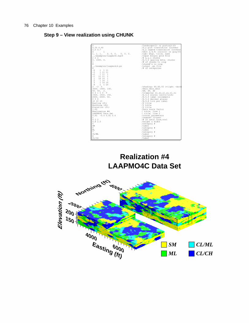
76 Chapter 10 Examples
Step 9 – View realization using CHUNK
0 /landscape(1) or portrait(0)0.35 0.40 /x,y plot translation (inches)2.0 0.7 /x,y legend translation (inches)4 1 /nbit 2,4,8; color(1) or gray(0)1. 1. 1. 0. 0. 0. 0. 0. 0. /rgb: bkgr, title, axes../examples/laapmo4c.bgr4 /input binary grid file2 2 2 /# x,y,z chunks0. 1000. 0. /X,Y,Z spacing betw. chunks1 /# of chunks to crop8 /chunk#’s to crop../examples/laapmo4c4.ps /output .ps file8 /# of categories-4 1 1 11-3 1 11 11-2 1 11 1-1 11 11 1 1 16 16 1 2 1 16 1 3 1 16 16 4 1 1 163 -3 0 /shading: XY,XZ,YZ (+light -dark)3000. 1400. 140. /Xmin,Ymin,Zmin50. 50. 2. /dX, dY, dZ0 4 1 5 0 9 /cropping: xl,xu,yl,yu,zl,zu1500. 1500. 150. /X,Y,Z scales (units/inch)2000. 2000. 50. /X,Y,Z label increments0 0 0 /X,Y,Z decimal places10 10 10 /X,Y,Z tics per labelEasting (ft) /X titleNorthing (ft) /Y titleElevation (ft) /Z title1.00 /Data scale factorRealization #4 / title, line 1LAAPMO4C Data Set / title, line 20.92 -0.4 0.92 0.4 /concat parameters1 /legend? (1=yes)4 2 2 /# of cats; nrow,ncol0.8 2.5 /height & width5 /category #SM /label6 /category #ML /label7 /category #CL/ML /label8 /category #CL/CH /label
150
Ele
vatio
n (f
t)
4000Easting (ft)
6000
4000
2000
Northing (ft)
200
Realization #4LAAPMO4C Data Set
SM
ML
CL/ML
CL/CH

References
Aarts, E., and Korst, J., 1989, Simulated annealing and Boltzmann machines: John Wiley &Sons, New York, 272 p.
Adobe Systems Incorporated, 1990, PostScript language reference manual, 2nd edition: Adison-Wesley, New York, 765 p.
Agterberg, F. P., 1974, Geomathematics: Elsevier, Scientific Publishing Co., Amsterdam, NewYork, 596 p.
Almeida, A. S., Journel, A. G., 1994, Joint simulation of multiple variables with a Markov-typecoregionalization model: Math. Geology, v. 26, no. 5, p. 565-588.
Carle, S. F., 1996, A transition probability-based approach to geostatistical characterization ofhydrostratigraphic architecture: Ph. D. dissertation, University of California, Davis, 248 p.
Carle, S. F., 1997a, Integration of geologic interpretation into geostatistical simulation: IAMG’97Proceedings of The Third Annual Conference of the International Association for Mathe-matical Geology, V. Pawlowsky Glahn (Ed.), International Center for Numerical Methods,Barcelona, Spain.
Carle, S. F., 1997b, Implementation schemes for avoiding artifact discontinuities in simulatedannealing: Mathematical Geology, v. 29, no. 2, p. 231-244.
Carle, S. F., and Fogg, G. E., 1996, Transition probability-based indicator geostatistics: Math-ematical Geology, v. 28, no. 4, p. 453-477.
Carle, S. F., and Fogg, G. E., 1997, Modeling spatial variability with one- and multi-dimensionalMarkov chains: Mathematical Geology, v. 28, no. 7.
Carle, S. F., Labolle, E. M., Weissmann, G. S., Van Brocklin, D., and Fogg, G. E., 1998, Con-ditional simulation of hydrofacies architecture: a transition probability/Markov approach,In Fraser, G. S., and Davis, J. M., Concepts in Hydrogeology and Environmental GeologyNo. 1, SEPM (Society for Sedimentary Geology) Special Publication, p. 147-170.
Carr, D. D., Horowitz, A., Hrarbar, S. V., Ridge, K. F., Rooney, R., Straw, W. T., Webb, W.,and Potter, P. E., 1966, Stratigraphic sections, bedding sequences and random processes:Science, v. 28, no. 3753, p. 89-110.
Deutsch, C. V., and Cockerham, P. W., 1994, Practical considerations in the application of sim-ulated annealing in stochastic simulation: Math. Geology, v. 26, no. 1, p. 67-82.
Deutsch, C. V., and Journel, A. J., 1992, Geostatistical software library and user’s guide: OxfordUniversity Press, New York, 340 p.
Doveton, J. H., 1971, An application of Markov chain analysis to the Ayrshire Coal Measuressuccession: Scott J. Geol., v. 7, no. 1, p. 11-27.
Ethier, V. G., 1975, Application of Markov analysis to the Banff Formation (Mississippian),Alberta: Math. Geology, v. 7, no. 1, p. 47-61.
Goodman, L. A., 1968, The analysis of cross-classified data – independence, quasi-independence,and interactions in contingency table with and without missing entries: American StatisticalAssociation Journal, v. 63, p. 1091-1131.
Goovaerts, P., 1996, Stochastic simulation of categorical variables using a classification algo-

rithm and simulated annealing: Math. Geology, v. 28, no. 7, p. 909-921.
Hattori, I., 1976, Entropy in Markov chains and discrimination of cyclic patterns in lithologicsuccessions: Math. Geology, v. 8, no. 4, p. 477-497.
Johnston, R. J., and Pattie, C. J., 1993, Entropy-maximizing and the iterative proportional fittingprocedure: Professional Geographer, v. 45, p. 317-322.
Journel, A. G., 1983, Nonparametric estimation of spatial distributions: Math. Geology, v. 1, no.1, p. 79-96.
Krumbein, W. C., 1968, Fortran IV computer programs for simulation of transgression and regres-sion with continuous-time Markov models: Computer Contribution 26, Kansas State Geologi-cal Survey, p. 1-18.
Krumbein, W. C., and Dacey, M. F., 1969, Markov chains and embedded Markov chains in geology:Math. Geology, v. 1, no. 1, p. 79-96.
Lin, C., and Harbaugh, J. W., 1984, Graphic display of two- and three- dimensional Markov com-puter models in geology: Van Nostrand Reinhold, New York, 180 p.
Miall, A. D., 1973, Markov chain analysis applied to an ancient alluvial plain succession: Sedi-mentology, v. 20, no. 3, p. 347-364.
Noyes, C. D., 1990, Hydrostratigraphic analysis of the Pilot Remediation Test Area, LLNL, Liv-ermore, California: unpubl. Masters Thesis, University of California, Davis.
Politis, D. N., 1994, Markov chains in many dimensions: Adv. Appl. Prob., v. 26, no. 3, p.756-774.
Qualheim, B. J., 1988, Well log report for the LLNL ground water project 1984-1987: LawrenceLivermore National Laboratory, UCID-21342 (updated 1989 and 1993).
Press, W. H., Teukolsky, S. A., Vetterling, W. T., Flannery, B. P., 1992, Numerical recipes in FOR-TRAN: Cambridge Univ. Press, New York, 963 p.
Schwarzacher, W., 1969, The use of Markov chains in the study of sedimentary cycles: Math.Geology, v. 12, no. 3, p. 213-234.