THE TAXATION OF DISCRETE INVESTMENT

CHOICES

Michael P. DevereuxRachel Griffith

REVISION 2THE INSTITUTE FOR FISCAL STUDIES

Working Paper Series No. W98/16

1

The taxation of discrete investment choices

Michael P. Devereux

Warwick University and Institute for Fiscal Studies

Rachel Griffith

Institute for Fiscal Studies

February 1999

Abstract

Traditional analysis of the taxation of income from capital has focused on the impact oftax on marginal investment decisions; the principal impact of tax on investment isthrough the cost of capital, and is generally measured by an effective marginal tax rate. Inthis paper, we consider cases in which investors face a choice between two or moremutually exclusive projects, both of which are expected to earn at least the minimumrequired rate of return. Examples include the location decisions of multinationals, firms’choice of technology, and the choice of investment projects in the presence of bindingfinancial constraints. In these cases the choice depends on the effective average tax rate.We propose a measure of this rate and demonstrate its relationship to the conventionaleffective marginal tax rate. Estimates of both are presented and compared for domesticand international investment in Germany, Japan, the UK and USA between 1979 and1997.

JEL classification: H25, H32

AcknowledgementsThe authors would like to thank Stephen Bond and Michael Keen for helpful commentson earlier drafts of this paper. Responsibility for errors remains ours. This research wasfunded by the ESRC Centre for Microeconomic Analysis of Fiscal Policy at the Institutefor Fiscal Studies; Devereux was supported by a Leverhulme Trust fellowship.

CorrespondenceProfessor Michael P. Devereux, Department of Economics, Warwick University,Coventry, CV4 7AL, UK email: M.P.Devereux@warwick.ac.ukRachel Griffith, IFS, 7 Ridgmount Street, London WC1E 7AE, UK email:rgriffith@ifs.org.uk

2

1. INTRODUCTION

Since the seminal works of Jorgenson (1963) and Hall and Jorgensen (1967) the standard

approach to investigating the impact of taxation on firms’ incentive to invest has been to

examine its impact on the cost of capital - the minimum pre-tax rate of return on an

investment required by the investor. The vast majority of both theoretical and empirical

work focuses on the impact of taxation on marginal investment on the assumption that

all potential investment projects that earn at least the cost of capital will be undertaken.

However, in many circumstances investment choices do not correspond to the

framework adopted in this literature. Where an investor faces a choice between two or

more mutually exclusive projects that are expected to earn more than the minimum

required rate of return the choice of which project to undertake depends on the level of

the post-tax economic rent that would be earned from each project. The impact of tax in

this case is measured by the proportion of the pre-tax economic rent taken by the

government - the effective average tax rate. Conditional on choosing one of the projects,

the level of investment may be affected by taxation through the cost of capital in the

usual way. This distinction is analogous to the labour supply decision where it is well

known that the impact of tax on an individual’s incentive to participate in the labour

market is through the average tax rate, while the number of hours worked is affected by

the marginal tax rate.

In Devereux and Griffith (1998) it was shown that the effective average rate of corporate

income tax that a firm might expect to face on an investment project is an empirically

significant factor for US multinational firms choosing where within Europe to set up a

production facility. In the model in that paper, the firm expects to earn an economic rent

on its activity by exploiting some firm specific advantage, such as a patent, but due to

3

economies of scale in production it will not build more than one plant.1 The effective

marginal tax rate is relevant in determining the optimal scale of the investment

conditional on the location having been chosen. The choice of location depends on the

level of post-tax economic rent; the impact of tax is through its effect on this level,

determined by the effective average tax rate.

In this paper it is argued that this model has a broader application than simply firms’

location choices. For example, consider a firm that faces a choice between a number of

alternative means of production, with a suitable investment in R&D a production facility

may be made more automated, compared with a relatively labour-intensive production

process in the absence of the R&D. Conditional on choosing which strategy to

undertake, the effective marginal tax rate may affect the level of investment undertaken.

However, the firm will only follow the strategy that yields the highest post-tax level of

economic rent, which depends on the effective average tax rate. Another example is a

firm operating in a differentiated goods market, choosing the type or quality of good to

produce. If production of the goods is taxed differently - for example because they use

different qualities or quantities of inputs which are taxed differently - then the difference

in the effective average tax rates may affect the firms’ choice.

There are two common elements in these examples - the investor faces a choice between

mutually exclusive investment projects and at least two of these projects must be

expected to generate positive economic rent before tax. The mutually exclusive nature of

the investment projects may arise for different reasons, but is likely to require the

existence of economies of scale. In the first two examples above, it is assumed that the

1 A number of theoretical models, based loosely on the OLI framework of Dunning (1977,1981), have this

property. See for example, Caves (1996), Horstman and Markusen (1992) and Markusen (1995).

4

firm faces a given demand schedule, and is choosing between alternative ways of meeting

demand. By assumption, it would be less profitable for the firm to undertake more than

one of its strategic options. For example, the multinational may face fixed costs of setting

up in each location. Setting up in two locations would mean paying fixed costs twice,

which – for a given demand - is likely to imply a lower overall post-tax economic rent.

Similarly, in the second example, the R&D creates economies of scale - having

undertaken the R&D, it would be less profitable to use both the old and new

technologies, rather than only the new technology. In the third example it is assumed

that production of more than one variety is constrained by a given demand schedule.

The second common element of these examples is that at least two strategies must exist

which are expected to generate a positive economic rent before tax. If only one strategy

is expected to generate a positive economic rent then whether it should be undertaken

can be analysed without reference to other possible strategies (assuming non-negative tax

liabilities). This means that the firm must operate in conditions of imperfect competition.

The precise form of imperfect competition is not important; all that is required for the

tax on economic rent to play a role is that at least two mutually exclusive projects have

the potential to earn economic rent.

Previous empirical work using average tax rates has tended to treat them as an imperfect

approximation to the effective marginal tax rate and has measured them using accounting

or tax return data.2 These measures generally take the current tax liability as a proportion

of current income. Several problems arise in using the realised amounts to analyse

investment strategies. For example, accounting measures of average tax rates typically

consider the firm at a single point in time, reflecting investments made by the firm over

2 See, for example, Swenson (1994), Grubert and Mutti (1996) and Collins and Shackelford (1995).

5

many previous periods as well as the current period, the return on those investments and

the way in which they were financed. They may also reflect the dynamic tax position of

the firm; for example, in a year in which the firm earns high income it may not incur any

tax liability because earlier losses may be brought forward. Accounting data on tax

liabilities may also reflect tax payments in other jurisdictions in which the firm operates.

Using these accounting or tax return based measures to make international comparisons

is also problematic due to differences in accounting definitions and the timing of tax

payments.

This paper sets out a framework to analyse the impact of tax on firms’ choice between

discrete investment decisions. We propose a new measure of the effective rate of

taxation of investment projects, an effective average tax rate (EATR). This builds on the

standard approach to measuring the effective marginal tax rate (EMTR).3 This approach

developed, for example, by Auerbach (1979) and King and Fullerton (1984), and at the

international level by Alworth (1988), Keen (1991) and OECD (1991), considers the net

present value of the income stream from an investment and the net present value of the

cost of the investment.4 Setting these equal defines the marginal investment and the

required pre-tax rate of return can be derived. This type of approach permits the analysis

of the impact of current (and expected future) tax regimes on the net present value of a

new investment project. It also provides a useful tool for policy makers to analyse the

impact of the tax system in isolation from other economic factors. However, although

3 Notably King and Fullerton (1984), Alworth (1988), OECD (1991) and Keen (1991).

4 An alternative approach, taken for example by Fershtman et. al. (1997), is to estimate the impact of tax

changes econometrically.

6

quite complex elements of the tax system can be analysed, several assumptions about the

structure and financing of the investment must be made. A number of important real

world features, such as the tax planning activities of multinational firms, cannot be dealt

with completely.

To compute the EATR, the net present value of the income stream is derived for an

investment which earns a given pre-tax rate of return. The economic rent generated is

simply the difference between this value and the net present value of the cost of the

investment. In principle, the EATR can be measured as the proportionate difference

between the pre-tax and post-tax economic rent, for a given pre-tax rate of return.

However, in practice, we propose a slightly different measure for two reasons. First, such

a measure is undefined for an investment which is marginal pre-tax, and hence has a zero

pre-tax economic rent. Secondly, the proposed measure of the EATR has the attractive

property that, for a marginal investment, it is equal to the EMTR. It can therefore be

interpreted as summarising the distribution of tax rates for an investment project over a

range of profitability, with the EMTR representing the special case of a marginal

investment.

In the empirical section of this paper estimates of the EATR are presented for four

countries –Germany, Japan, UK and USA - over the period 1979-1997. An analysis of

how tax reforms in these countries have changed the shape of the tax schedule is given.

How these tax schedules might affect investment incentives and choices in a number of

situations is illustrated.

The structure of the remainder of the paper is as follows. The following section discusses

in more detail some circumstances in which the EATR is the appropriate measure for

investigating the impact of taxation on firms’ investment decisions. Section 3 sets out a

framework in which the EATR is then derived and analysed in a domestic context. This

7

is extended in Section 4 to the case of international investment. In section 5 empirical

values of the EATR for four countries are presented. Section 6 briefly concludes.

2. CONCEPTUAL FRAMEWORK

A number of situations are described in which the EATR may affect investment choices.

A simple framework makes it easier to highlight the common elements of these choices.

This framework can be extended in a number of directions to model any particular

choice in more detail.

Consider the profit-maximising behaviour of a single firm that faces two investment

opportunities, denoted strategies i = 1 2, . The precise form of the competition is not

crucial; however, the possibility of earning a positive pre-tax economic rent must exist.

The cost structure of each of the two strategies consists of an investment in a fixed asset,

Fi , and variable cost per unit of output. Denote the pre-tax net present value of the

stream of income net of variable costs as Yi*, where the asterisk indicates a pre-tax value.

The pre-tax economic rent, Ri* , associated with strategy i is assumed to be positive:

R Y Fi i i* *= - > 0. (2.1)

There are three options available to the investor: strategy 1, strategy 2, or both.

Undertaking both strategies would incur investment of F F1 2+ . Unless variable costs are

increasing with output, then any given output could be produced at lower cost by

following only one of the strategies. Only the case in which economies of scale rule out

undertaking both strategies is considered. Given this assumption, in the absence of tax,

the investor would choose the strategy with the highest level of Ri* (as long as this is

non-negative). Defining a binary indicator X i* of whether strategy i is chosen in the

absence of tax, it will take the values,

8

{ }otherwise 0

,max if 1 *2

*1

** RRR

X ii

== (2.2)

Now consider how tax will affect this choice. The statutory corporate income tax rate is

denoted t i and the net present value of tax allowances per unit of investment is denoted

Ai . Assume that income is taxed and variable costs are fully tax deductible. If the level of

output is independent of the size of the investment (that is, Fi is a fixed cost) the full

deductibility of variable costs implies that the optimal level of output in the presence of

tax and conditional on choosing strategy i, Yi , is the same as its level in the absence of

tax, *iY . This implies that the net present value of the income stream becomes

( ) *1 ii Yτ− , and the net cost of the investment is ( ) ii FA−1 . The post-tax economic rent

of strategy i is therefore:

( ) ( ) iiiii FAYR −−−= 11 *τ . (2.3)

Post-tax the investor will choose the project with the highest level of Ri (again, as long as

this is non-negative). That is, defining a binary indicator, X i , of whether strategy i is

chosen in the presence of tax, it will take the values:

{ }otherwise 0

,max if 1 21 RRRX i

i

== (2.4)

It is straightforward to generalise this to the case in which output depends on the level of

investment. In this case, the optimal level of investment for any strategy, conditional on

having chosen that strategy, will be determined by the equality of marginal revenue and

marginal cost, implying a role for the effective marginal tax rate (EMTR). In this case

( ) ( ) iiiii FAYR −−−= 11 τ , and the EATR is determined with reference to Yi rather than

to Yi*. In this case, the EATR cannot summarise all of the difference between investment

choices in the absence of tax and the presence of tax. However, this is true of almost all

9

such measures. For example, it is standard to compute the EMTR with reference to the

actual required post-tax rate of return rather than the required rate of return in the

absence of tax.

Neglecting the distinction between Yi and Yi*, the key issue is whether the tax system can

affect the ranking of projects, that is whether X Xi i* π . Clearly this is possible if the

projects face different tax regimes, as is often the case. However, it can also be true even

if all projects face an identical tax regime, represented by t t t= =1 2 and A A A= =1 2 .

For the case where Y Yi i= * the necessary and sufficient condition for tax to change the

ranking of the projects, R R1 2* *> but R R1 2< , is that

( )( ) ( )( ) ( )( )21*

2*

121 111 FFAYYFF −−<−−<−− ττ . (2.5)

In this case, where the tax system is the same for the two projects, the ranking of

projects can only change if the fixed costs are unequal, F F1 2π , and if they cannot be

fully depreciated in the first period, that is A < t .

For empirical and policy purposes it is useful to be able to summarise the impact of tax

on the ranking of projects in a single measure. The effective average tax rate (EATR)

provides such a measure. The most obvious approach would be to define an effective

average tax rate, iℑ , such that ( ) iii RR =ℑ− *ˆ1 implying that ( )*

*ˆ

i

iii R

RR −=ℑ . With

this definition, the choice of the highest Ri is identical to the choice of the highest

( ) *ˆ1 ii Rℑ− . However, this measure suffers from the disadvantage that it is undefined for

investment projects which are marginal pre-tax, that is for Ri* = 0 .

Instead, we define effective average tax rate as the difference between the pre and post-

tax economic rent scaled by the net present value of the pre-tax income stream:

( ) **iiii YRR −=ℑ . In choosing between strategies, simply applying this rate to Ri

*

10

would not be appropriate. However, it is straightforward to compare two strategies, as

long as Yi* and Fi are both known. Choosing the strategy with the highest Ri is

equivalent to choosing the strategy with the highest R Yi i i* *- ¡ . Equivalently, R R1 2> iff

( ) ( ) ( )21*

22*

11 11 FFYY −>ℑ−−ℑ− .5

A number of economic situations in which the EATR is the appropriate measure of the

impact of corporate income taxation on firms’ incentives to invest are now considered.

2.1 Alternative locations of production

Consider a firm which has decided to serve a foreign market, and which could do so by

producing at home and exporting (strategy 1), or by producing in the foreign location

(strategy 2). It has an advantage over local firms in that it owns a superior technology, so

that there is a barrier to other firms entering the market. It will choose to produce in the

location in which it will earn the higher post-tax economic rent.

There may be additional costs to setting up abroad, relative to expanding existing home

capacity so that fixed costs of strategy 1 are lower than 2, 21 FF < . On the other hand,

exporting the product to the foreign location is costly, so that variable costs are higher

under strategy 1, 21 YY < . The ranking of these two strategies therefore depends on the

relative size of fixed versus variable costs. Tax regimes differ across countries so that,

t t1 2π and/or A A1 2π . It is clearly possible for tax to change the ranking of projects so

that , for example, R R1 2* *< but R R1 2> so that in the absence of tax the firm would

prefer to produce abroad, but in the presence of tax the firm would prefer to produce at

home.

5 If the optimal level of output is affected by tax, then this condition should use Yi rather than Yi*.

11

Models of the location decision of multinationals, such as Horstman and Markusen

(1992), have employed this framework. This example can easily be extended to many

possible foreign locations. Conditional on deciding to produce abroad, a firm may face a

number of alternative sites. Examples would include a US car manufacturer deciding

where to produce in Europe in order to serve the European market, or a Korean

electronics producer choosing a North American location from which to enter the North

American market. Differences in the tax regimes facing the firm may alter the ranking of

alternatives. A model of this type was developed in Devereux and Griffith (1998), in

which the optimal level of output under each strategy depends on the effective marginal

tax rate, but the choice between strategies depends on the ranking of post-tax economic

rent, and hence on the effective average tax rate.

2.2 Alternative production technologies

The different fixed costs, 1F and 2F , may reflect investment in alternative production

technologies. For example, strategy 1 may represent high expenditure on R&D which is

expected to yield a more automated and cheaper production process. By contrast,

strategy 2 could mean lower investment in R&D. This would imply that fixed costs are

higher under strategy 1, F F1 2> , but variable costs lower, 21 YY > . Either strategy would

be more profitable than following both. The tax system can change the ranking of the

two strategies; which strategy is chosen will depend on the post-tax level of economic

rent which is affected by the effective average tax rate.

A central concern in the literature on effective marginal tax rates has been the distortions

which might be introduced by differential taxation of alternative forms of production,

which might induce investors to choose a sub-optimal mix of assets. This has generally

12

been measured by comparing the costs of capital for investment in alternative assets.6

But this approach relies on the assumption that the mix of assets can be continuously

varied, with the outcome that the quantity of each asset is chosen so that its marginal

product is equal to its cost of capital. By contrast, in the framework presented here it is

assumed that there are a limited number of production strategies from which to choose,

each strategy corresponding to a particular asset mix.

2.3 Choice of product type or quality

Consider a firm that is operating in a differentiated product market, choosing between

supplying a product of either low or high quality. Suppose that the two products are

highly substitutable in demand so that the additional revenue derived from producing

both products would be less than the additional cost. The tax system could affect the

ranking of the post-tax economic rent and thus distort the firm’s choice between the

goods. An extreme example would be the choice of what property to build on a piece on

land (where there is no possibility of constructing more than one type of building) –

whether, for example, to build private houses, an apartment block or a hotel.

Empirical work looking at the impact of tax on product choice has tended to focus on

the impact of excise and commodity taxes.7 In this paper we focus on the impact of

corporate income taxes on firms’ investment choices. Because revenue from different

6 For example,Goolsbee (1998) develops a model where the tax treatment of investment affects firms’choice of quality of investment good. This is because tax applies only to the purchase and installation ofthe capital good, while future maintenance and training costs are not counted as part of the investment butare expensed when incurred. Goolsbee’s results indicate that when the cost of capital falls a largerproportion of high quality investment goods are purchased.

7 For example, Cremer and Thisse (1994) show that an increase in commodity taxation in a verticallydifferentiated product market, where firms compete on price, changes the quality mix of productsprovided. Fershtman et. al. (1997) look at the impact of tax in the Israeli automobile market, which theyassume to be oligopolistic. They simulate the affect of tax on firms’ behaviour and are thus able to showhow the imposition of the tax has affected the profile of goods sold and their relative prices.

13

sources is generally taxed at the rate same, the impact of corporate tax on product choice

will be through the differential treatment of inputs, for example due to difference

depreciation allowances.

2.4 Choice of investment given financial constraints

There is a sizeable literature investigating the extent to which firms’ investment plans are

constrained by the availability of financial capital, either from internal or external

sources.8 One important effect of the average tax rate is the impact it has on the amount

of internal funds available for investment. The size of internal funds will clearly depend

on the average tax rate. But this is a different concept to the one dealt with in this paper

– our measure is forward-looking and based on the present value of returns and costs of

a new investment.

The existence of financial constraints introduces a role for the measure developed in this

paper. Financial constraints may make it difficult for the firm to undertake all of its

potentially profitable investment projects. Suppose that there is an absolute limit on the

funds which can be raised for new investment. The firm will choose only those projects

which are expected to yield the highest post-tax economic rent based on a ranking which

may be affected by taxation.

8 See, for example, the survey by Hubbard (1998).

14

3 THE EFFECTIVE AVERAGE TAX RATE ON DOMESTIC

INVESTMENT

This section describes the proposed measure of the effective average tax rate (EATR) as

it applies in a domestic setting. A standard model is set up which can incorporate discrete

investment. In the next section this is extended to an international setting. The properties

of the EATR in the international case are equivalent to those for the domestic case.

Consider a value-maximising firm. In the tradition of King (1974), the value of the firm

can be derived from the capital market equilibrium condition. Risk is ignored. The value

of the firm in period t is the net present value of the post-tax income stream, given by

tV :

)NVV(zVNDc

)m(iV)m( tttttt

d

ti −−−+−

−−

=− ++ 111

11 (3.1)

where i is the nominal interest rate, tD is the dividend paid in period t, tN is new

equity issued in period t, im is the personal tax rate on interest income, dm is the

personal tax rate on dividend income, c is the rate of tax credit available on dividends

paid, and z is the accruals-equivalent capital gains tax rate. The right hand side of (1) is

the return from purchasing the equity of the firm; in the absence of arbitrage

opportunities and risk, this is equal to the return from lending tV ; hence tV represents

the value of the firm’s equity. Rearranging (1) yields an expression for tV :

{ } )/(VNDV tttt ρ++−γ= + 11 (3.2)

where )z)(c/()m( d −−−=γ 111 is a term measuring the tax discrimination between

new equity and distributions and )z/(i)m( i −−=ρ 11 is the shareholders’ nominal

discount rate.

15

Net dividends paid by the firm can be found from the equality of sources and uses of

funds in each period:

ttttttt TBiBIKQND −+−+−=− −− 11 )1()( (3.3)

where )K(Q t 1− is output in period t, which depends on the beginning of period capital

stock, 1−tK , tI is investment, tB is one-period debt issued in period t and tT is the tax

liability. Choosing the appropriate units of capital and output, the prices of output and

capital goods are normalised to unity in period t. The tax liability is defined as:

{ })()( 111Ttttt KIiBKQT −−− +−−= φτ (3.4)

where τ is the statutory tax rate, φ is the rate at which capital expenditure can be offset

against tax, and TtK 1− is the tax-written-down value of the capital stock at the end of

period t defined as

tTt

Tt IKK +−= −1)1( φ . (3.5)

It is useful to define the net present value of allowances per unit of investment as A,

where9

φ+ρρ+τφ

=

+

ρ+φ−

+

ρ+φ−

+τφ=)(

...A1

1

1

1

11

2

. (3.6)

The net cost of one unit of physical investment in period t is therefore )1( A− . Finally,

the equation of motion of the capital stock is standard:

ttt IK)(K +δ−= −11 . (3.7)

9 This expression corresponds to the case of exponential, or declining balance, depreciation. Theexpression is for straight line depreciation is given by equation (A.11) in Appendix A.

16

3.1 Measuring effective tax rates

Measures of effective marginal and average tax rates on domestic investment can now be

derived. The standard approach in deriving the cost of capital, and hence the effective

marginal tax rate, EMTR, is to consider a perturbation of the capital stock in one period,

say period t. Setting economic rent equal to zero at the margin, dV dKt t = 0, defines the

cost of capital and permits the optimal capital stock in period t to be found. We follow

the sprit of this approach in developing a measure of the effective average tax rate,

EATR. Consider an investment which increases the physical capital stock of the firm by

one unit in period t only, so that the change is 1=tdK and tsdK s ≠∀= 0 . This

requires an increase in investment in period t of one unit: 1=tdI and a reduction in

investment in period t+1 such that ( )πδ +−−=+ 1)1(1tdI , where π is the nominal

increase in prices between periods t and t+1. The addition to tK increases output in

period t+1. This generates a change in output of δ+=+ pdQt 1 , where p represents the

financial return and δ reflects the one-period cost of depreciation, and a change in net

revenue of ( ) ( )( )πδπ ++=++ 111 pdQt . Here we have simplified the analysis by

assuming that π is a general inflation rate common to capital and output. We therefore

abstract from specific inflation of the price of capital, although this would be

straightforward to introduce.

Modelling of the financial policy of the firm is typically arbitrary in models which

construct measures of the effective marginal tax rate. For example, the well-known

expressions used by King and Fullerton (1984) imply financial cash flows which are

difficult to justify by modelling a simple one period investment. The approach here is

implicitly that of setting financial constraints – in particular, non-negativity constraints on

dividend payments, new equity issues and debt issues. Edwards and Keen (1984)

17

demonstrate that in such a model the cost of capital depends on whether these

constraints are binding in each of period t and period t+1. Given these three constraints

in each period implies that there may be nine different combinations of financing the

investment and receiving the return from the investment. In order to generate measures

that are close to those commonly used, it is necessary to assume that the constraint on

non-negative dividends is not binding in period t+1. Since dividends are the residual in

this model, this implies that, at the margin, any return from the investment made in

period t is distributed as a dividend in period t+1.10 In the case of new equity, most tax

systems treat a repurchase of equity at its original price to be a repayment of capital

which is not taxed. It is assumed that the firm takes advantage of this opportunity for the

case of new equity finance. Any payment to shareholders above this amount is taxed as a

dividend, and is therefore treated here as a dividend payment. This reduces the number

of possibilities to three, corresponding to the cases when the investment is financed by

retained earnings, new equity and debt in period t.

Rather than model the constraints explicitly, changes to these forms of finance in periods

t and t+1 are considered. The cases for domestic investment are shown Table 3.1, where

tdN and tdB are the changes in new equity and debt respectively in period t ( tF is

defined below). In the case of retained earnings, the investment is financed by a

reduction in dividend payments in period t; hence debt and new equity issues are

unaffected. In the case of new equity finance the firm issues new equity in period t of

φτ−1 ; this finances a physical investment of 1 since an immediate tax allowance worth

φτ can be claimed. As note above, in period t+1 the firm repurchases that equity at the

10 This assumption is also followed elsewhere; see, for example, Keen (1991) and Devereux, Keen and

Schiantarelli (1994).

18

original price. In the case of debt financed investment the firm borrows φτ−1 in period

t and repays that amount plus interest (at rate i) in period t+1.

Table 3.1: Financial constraints on investment by source of finance

RetainedEarnings

sdBdN stst ∀== ++ 0 0=⇒ tF

New Equity sdB st ∀=+ 0

ttt dNdNdN −=φτ= +1 ; -1

1 0 >∀=+ sdN st

)1()1(

)1(φτ

ργρ

−+

−−=⇒ tF

Debt sdN st ∀=+ 0

0 0 ; 1 >∀=φτ−= + sdBdB stt{ })1(

)1(

)1(τρ

ρφτγ

−−+−

=⇒ iFt

In general, define tR to be the net present value of this investment - equal to the net

present value of the economic rent generated. In general, this is defined as:

∑∞

=

++

+

+−

=

++=+=

0

1

)1(

)1(

ss

stst

ttttt

dNdD

dVdNdDdVR

ργ

ρ

. (3.8)

To implement this definition consider the change in dividends, stdD + implied by (3.3)

and substitute into that expression the values of the change in investment in periods t

and t+1, the change in net revenue in period t+1, and changes in the source of finance

from Table 2.3. The resulting expression can be usefully split into two parts: (i) the rent

attributable to investment financed by retained earnings, REtR , and (ii) the additional cost

of raising external finance, tF , defined in (3.10) and Table 3.1. In sum, tREtt FRR += .

The two elements of the post-tax economic rent are:

( ) { })1)(1)(1()1)()(1(1

1 ApAR REt −−++−++

++−−= δπτδπ

ργ

γ (3.9)

and

19

ρ+−γ−−

ρ+τ−+

−γ=1

111

1

111 ttt dN)(

)(idBF . (3.10)

This framework easily permits the derivation of standard measures of the cost of capital:

set 0=tR and solve for the marginal financial rate of return, denoted p~ :

{ } .)1)(1(

)1()1(

)1)(1(

)1(~0 δπτγ

ρππδρ

πτ−

+−+

−−+++−

−=⇒= t

t

FApR (3.11)

The tax inclusive effective marginal tax rate (EMTR) is given by p~/)sp~(EMTR −= ,

where s is the post-tax real rate of return to the shareholder:

π+π−−

=1

1 i)m(s

i

. (3.12)

This EMTR can be illustrated in the case in which 0== zm i and hence i=ρ , the

nominal interest rate. Define r to be the real interest rate: )i())(r( +=π++ 111 . Then

the cost of capital for investment financed by retained earnings ( 0=tF ) becomes:

{ } δ−δ+τ−

−= r

)(

)A(p~RE

1

1 (3.13)

and the equivalent EMTR is:

)()A)(r(

)A)(r(EMTR RE

τ−δ−−δ+−τδ+

=11

. (3.14)

The general expression for the cost of capital in (3.11) is similar to measures of the cost

of capital derived elsewhere. There are two principal difference from the King and

Fullerton (1984) formulation. First, here the net present value of depreciation allowances,

A, is derived using the shareholders’ discount rate, p~ . Second, the impact of alternative

forms of financing is limited to periods t and t+1 in the case of new equity and period t

in the case of debt. This implies that the allowance in period t - that is φτ - is important,

20

rather than simply the net present value of allowances, A. We choose this approach on

the grounds that the financial flows implied by the King and Fullerton formulation for

new equity are very difficult to justify.

The effective average tax rate, EATR, is defined for p~p ≥ , as described in the previous

section, by dividing the difference between pre- and post-tax economic rent by the net

present value of the income stream. Evaluating the pre-tax economic rent at the interest

rate in the presence of tax yields an expression for the pre-tax economic rent, *tR of:

{ }

r

rp

pi

Rt

+−

=

−+++++

+−=

1

)1)(1())(1(1

11* δπδπ

(3.15)

Note that in the absence of tax, the additional terms due to financing by new equity or

debt (the pre-tax equivalent of tF ) both have a net present value of zero and so do not

affect the pre-tax economic rent.

As noted above, a natural measure of the EATR would be the proportional difference

between *tR and tR ie. *

tt*t R/)RR( − . However, this is undefined when 0=*

tR .

Instead, we scale the difference )RR( t*t − by the net present value of the pre-tax

income stream, net of depreciation: ).r/(p +1 Hence the measure of the EATR

proposed here is:

rp

RREATR t

*t

t

+

−=

1

. (3.16)

A general expression for the EATR which uses the value of tR from (3.9) and (3.10) and

the value of *tR from (3.15) is given in the Appendix in expression (A.15). Here we

illustrate its properties in the absence of personal taxes on interest income and capital

21

gains: 0== zm i , implying that i=ρ . Substituting these values into the expression for

tR and simplifying yields:

{ } tt F)A)(r())(p(r

R +−δ+−τ−δ++γ

= 111

. (3.9a)

Combining (3.16), (3.9a) and (3.15) and rearranging yields:

[ ]{ }p

rFAArEATR t

t

)1()()1(1)1(1

++−−−−−−−=

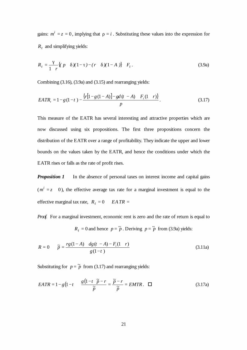
τγδγτγ . (3.17)

This measure of the EATR has several interesting and attractive properties which are

now discussed using six propositions. The first three propositions concern the

distribution of the EATR over a range of profitability. They indicate the upper and lower

bounds on the values taken by the EATR, and hence the conditions under which the

EATR rises or falls as the rate of profit rises.

Proposition 1 In the absence of personal taxes on interest income and capital gains

( 0= zm i ), the effective average tax rate for a marginal investment is equal to the

effective marginal tax rate, EATRRt =⇒= 0

Proof. For a marginal investment, economic rent is zero and the rate of return is equal to

0=tR and hence p~p = . Deriving p~p = from (3.9a) yields:

)1(

)1()()1(~0τγ

τδγγ−

+−−+−=⇒=

rFAArpR t (3.11a)

Substituting for p~p = from (3.17) and rearranging yields:

( ) ( )EMTR

p

rp

p

rpEATR =

−=

−−+−−= ~

~

~

~111

τγτγ . o (3.17a)

22

Proposition 2 In the absence of personal taxes on interest income and capital gains

( 0== zm i ), the effective average tax rate for a very profitable investment approaches

an “adjusted” statutory tax rate: )(EATRp τ−γ−→⇒∞→ 11 .

Proof Immediate from (3.17). o

Proposition 3 In the absence of personal taxes on interest income and capital gains

( 0== zm i ), the effective average tax rate increases with profitability if and only if the

“adjusted” statutory tax rate exceeds the effective marginal tax rate, ie.

)(EMTRpEATR τ−γ−<⇔>∂

∂ 110 .

Proof. Differentiating (3.17) with respect to p implies:

[ ] 01110 >++−τγδ−−γ−⇔>∂∂ )r(F)A()A(rpEATR .

Using the expression for p~ in (3.11a) this can be written as:

prpEATR ~)1(0 τγ −>⇔>∂

∂ .

Substituting using the expression p~/rEMTR −= 1 and rearranging yields:

)(EMTRpEATR τ−γ−<⇔>∂

∂ 110 . o

These three properties of the EATR are attractive. The EATR can be seen as reflecting

the whole schedule of effective tax rates over the range of profitability from a marginal

investment, where EATR=EMTR, to a very high rate of profitability, where the EATR

tends towards the statutory tax rate, adjusted for the tax treatment of dividends,

)( τ−γ− 11 . The EMTR and the adjusted statutory tax rate thus represent the upper and

lower bounds of values of the EATR.

23

Three further features of the EATR are worth noting, in comparison with well-known

properties of the EMTR. First, Auerbach (1979) showed that the EMTR for investment

financed by retained earnings is independent of the taxation of dividends paid to the

shareholder. This does not hold for the EATR at positive values of economic rent.

Proposition 4 In contrast to the EMTR, the EATR is not independent of the tax rate on

dividends ( γ ) for an investment financed by retained earnings.

Proof. Immediate from (3.17). Adding personal taxes clearly does not affect this

dependence. o

The remaining two propositions describe the value of the EATR for two special forms

of taxation.

Proposition 5 In the absence of personal taxes on interest income and capital gains

( 0== zm i ), a “neutral” business tax, with EMTR=0 and a classical tax system ( 1=γ ),

has an EATR with a lower bound of zero for a marginal investment and approaches the

statutory tax rate for a very profitable investment.

Proof. Immediate from Propositions 1 and 2, given EMTR = 0 and g = 1.o

Proposition 6. In the absence of personal taxes ( 0=== di mzm ), for a domestic tax

system which gives relief for true economic depreciation but no relief for the cost of

finance, the EATR is equal to the EMTR and also equal to the statutory tax rate, τ ,

irrespective of profitability.

Proof. A tax system that give relief for true economic depreciation implies that

δ+δτ

=

+

+δ−

++

δ−+

+δτ

=r

...rrr

A2

11

11

11

. Substituting this value, and 0=F , into

(3.17) yields )/(rp~ τ−= 1 which implies that τ=EMTR . In the absence of personal

24

taxes on dividends and any relief for equity finance, then 1=γ . This implies that both

the lower and upper bounds on the EATR are equal to τ , and hence

τ== EMTREATR .o

4 THE EFFECTIVE AVERAGE TAX RATE ON

INTERNATIONAL INVESTMENT

The approach used in the previous section can be used also to measure the effective

marginal and average tax rates for an international investment. In this section we sketch

the derivation of these effective tax rates; the detailed measures are given in the

Appendix. The basic approach is to consider a parent firm located in the “residence”

country j which undertakes investment in the “source” country n through a wholly-

owned subsidiary. The parent firm is assumed to be owned by shareholders located in j.

We take account of taxes levied by the government of n on income earned by the

subsidiary in n , corporate taxes levied by the government in j on the same income and

personal taxes levied by the government in j on the shareholders. The precise nature of

the combined tax system is similar to that in Keen (1991) and OECD (1991) and is

summarised in the Appendix. However, it is useful to here to note two tax parameters:

jnσ is the overall corporate tax rate levied on dividend payments from the subsidiary to

the parent and jnω is the overall corporate tax rate levied on interest payments from the

subsidiary to the parent. In general, tax parameters in n are equivalent to those defined in

the previous section; to note that they apply to country n they carry a subscript n.

Suppose that the previous section refers to the domestic activities of the parent firm.

Allowing for this firm to have a foreign subsidiary does not affect the general expression

for the value of the firm in (3.2); this remains the firm’s maximand. However, the

25

sources and uses of funds statement (3.3) must be extended to allow for financial flows

to and from the subsidiary, together with any consequential tax effects. This includes

new equity in the subsidiary provided by the parent and lending to the subsidiary by the

parent. It also includes dividends and interest received by the parent, net of taxes paid to

the source country government. Finally it includes further taxes due in the residence

country on the income earned in the source country. These flows are shown in detail in

the Appendix.

As in the domestic case, we consider a perturbation in the capital stock of the firm – in

this case the subsidiary – in period t. This is achieved by changing investment in the

subsidiary in periods t and t+1 in the same way as in the previous section. We consider

three ways in which the subsidiary finances the increase in investment, again

corresponding to domestic case: retained earnings, new equity issued to the parent and

borrowing from the parent. In the latter two cases, we in turn allow the parent to choose

between the three sources of finance. We do not consider the case of borrowing in the

source country n; this would be a straightforward extension.

The net present value of the economic rent generated by the perturbation of the

subsidiary’s capital stock takes the same form as for the domestic case. Dropping time

subscripts, we label this nREnn FFRR ++= where for convenience we have dropped

the time subscript. The first element, REnR , corresponds to the economic rent generated

by a perturbation in the capital stock financed by retained earnings. The second element,

F summarises the net present value of the cash flows associated with new equity and

debt financing of the parent firm, and is identical to the expression in (3.10). The third

element, nF , summarises the net present value of cash flows associated with new equity

and debt finance of the subsidiary. The first and third terms have the following values

(see the Appendix for details.):

26

( )( )

{ })1)(1)(1()1)()(1(1

)1(

11

nnnnnjn

jnREn

AEpE

AR

−−++−+++

−+

−−−=

δπτδπρ

σγ

σγ(4.1)

and

[ ]{ }

+−−−−−+

+=

ργσγσωτσ

ργ

1111

1

EdNi))(i(E

dBF tjnjnjnnjn

tn . (4.2)

where variables have the same meaning as in the previous section, except where the

subscript n represents the source country. The exchange rate is normalised at unity in

period t and takes the value E in period t+1. The expression 1)1( −+ nE π therefore

reflects the nominal price change expressed in the currency of the residence country.

These expressions correspond closely to (3.9) and (3.10). The new variables jnσ and

jnω reflect the impact on overall tax liabilities of changing the flows from the subsidiary

to the parent of dividends and interest respectively. Thus, for example, all cash flows

associated with an investment in the subsidiary financed by retained earnings directly

affect the flow of dividends (which are reduced by financing the investment in period t,

but increased by the return on the investment in period t+1): in both cases the value to

the ultimate shareholder is therefore multiplied by the factor jnσ−1 . Similarly, for given

investment, flows of new equity and debt to and from the subsidiary also have a direct

impact on the flow of dividends and hence introduce jnσ . Payment of interest from the

subsidiary to the parent – assumed to be at the market interest rate i – introduces the net

tax rate on such flows: jnω .

As in the domestic case, this framework permits derivation of measures of the cost of

capital for international investment. Define the cost of capital to be the real return in the

27

home currency for which 0=nR . Denote this )/(p)(E~nnn π+π+=ρ 11 . It is

straightforward to show that this is:

[ ]{ }

)1(

)1(

)1)(1)(1(

)1)((

1)1()1()1)(1(

)1(~0

ππδ

τπσγρ

ππδρτπ

++

−−++

++−

−+−++−+

−=⇒=

n

njn

n

nnn

nnn

EFF

EEA

pR

(4.3)

The EMTR for an international investment is nEMTR = nn p~/)sp~( − , where s is the

post-tax rate of return to the shareholder.

We follow the same approach as for the domestic case in defining a measure of the

EATR. In the absence of tax, 0== nFF , and so the pre-tax economic rent (again

evaluated at the same interest rate, i) is

{ }i

ipER nn

n ++−++

=1

)1()1)(1(* π. (4.4)

We define the EATR for international investment as:

ipERR

EATRnn

nnn

++

−=

1)1(

*

π (4.5)

where the denominator is again the net present value of the income stream from the

perturbation to the capital stock of the subsidiary, *nR is defined in (4.4) and nR is

defined as the sum of (4.1), (3.10) and (4.2). A detailed expression for this EATR is given

in the Appendix.

However, to give more intuition here, note that for the special case of purchasing power

parity, )()(E n ππ +=+ 11 , and no personal taxes in the residence country on interest

income or capital gains ( 0== zm i ), these expressions simplify to:

28

r

rpR nRE

n +−

=1

, (4.6)

{ } nnnnjn

n FF)A)(r())(p(r

)(R ++−+−−+

+

−= 11

1

1δτδ

σγ(4.7)

and

[ ]{ }n

nnnjnnjn

njnn

nnn

p

rFFAArr

pRR

EATR

)1)(())(1()1)(1(1

)1)(1(1

1

*

+++−−−−−−−

−−−=

+

−=

τσδγσγ

τσγ

(4.8)

This expression is similar to that for the domestic case, given in (3.17). There are three

main differences. First, most of the tax variables refer to the source country, n, rather

than the residence country. Second, an additional term jnσ−1 appears in several places,

reflecting the additional tax on dividends paid by the subsidiary to the parent. Third,

there is an additional financing term, reflecting the tax implications of financing the

subsidiary as well as the parent.

This measure of the EATR for international investment has equivalent properties to that

for the domestic investment described above. We briefly repeat the first four in this

context.

Proposition 1a In the absence of personal taxes on interest income and capital gains

( 0== zm i ), the effective average tax rate for a marginal international investment is

equal to the effective marginal tax rate, nnn EMTREATRR =⇒= 0 .

Proof. This is most easily seen for the case of purchasing power parity, although the

proposition is not limited to this case. In this case, simplifying (4.3) for

)()(E n ππ +=+ 11 yields:

29

))((

)r)(FF()A)(()A)((rp~R

njn

nnnjnnjnnn τσγ

τσδγσγ

−+

++−−−+−−=⇒=

11

11110 (4.3a)

Using this expression, for a marginal investment, (4.8) can be written as

{ }n

njnnnjnn p~

))((p~r))((EATR

τ−σ−γ−−τ−σ−γ−=

11111 .

Rearranging yields:

nn

nn EMTR

p~rp~

EATR =−

= .

In the absence of purchasing power parity, but with 0== zm i , using the definition of

np~ from (4.3) yields the same result. o

Proposition 2a In the absence of personal taxes on interest income and capital gains

( 0== zm i ), the effective average tax rate for a very profitable investment approaches

an “adjusted” statutory tax rate: )1)(1(1 njnnn EATRp τσγ −−−→⇒∞→ .

Proof Immediate from (4.8). The absence of purchasing power parity would clearly not

affect this result.o

Proposition 3a In the absence of personal taxes on interest income and capital gains

( 0== zm i ), the effective average tax rate increases with profitability if and only if the

“adjusted” statutory tax rate exceeds the effective marginal tax rate, ie.

))((EMTRpEATR

njnnn

n τ−σ−γ−<⇔>∂∂ 1110 .

Proof. This is again most easily shown for the case of purchasing power parity, although

this is not necessary for the proposition to hold. Differentiating (4.8) with respect to np

implies:

30

[ ] 0111110 >+++−−−−−−⇔>∂∂ )r)(FF()A)(()A)((rpEATR

nnnjnnjnn

n τσγδσγ

Using the expression for np~ in (4.3a) this can be written as:

njnn

n p~))((rpEATR τ−σ−γ>⇔>∂

∂ 110 .

Substituting the expression: nn p~/rEMTR −= 1 and rearranging yields:

))((EMTRpEATR

njnnn

n τ−σ−γ−<⇔>∂∂ 1110 . o

The EATR for international investment can thus also be seen as reflecting the whole

schedule of taxes from a marginal investment to a highly profitable investment. Finally,

just as the EATR for a retained-earnings financed domestic investment depends on the

dividend tax rate γ , so the EATR for a retained earnings-financed international

investment also depends on the tax rate on dividends paid from the subsidiary to the

parent, jnσ .

Proposition 4a In contrast to the EMTR,11 the EATR for international investment

financed by retained earnings is not independent of the tax rate on dividends paid by the

subsidiary to the parent ( jnσ ).

Proof. Immediate from (4.8). o

5 EMPIRICAL APPLICATION

In this section some of the properties of the EATR are examined using data on the tax

treatment of investment in six assets in four countries - Germany, Japan, the UK and the

11 See Hartman (1985).

31

USA – over the period 1979-1997. A description of the tax systems and the assumptions

used to calculate the effective tax rates is given in the Appendix B.12

5.1 Tax schedules in Germany, Japan, the UK and USA

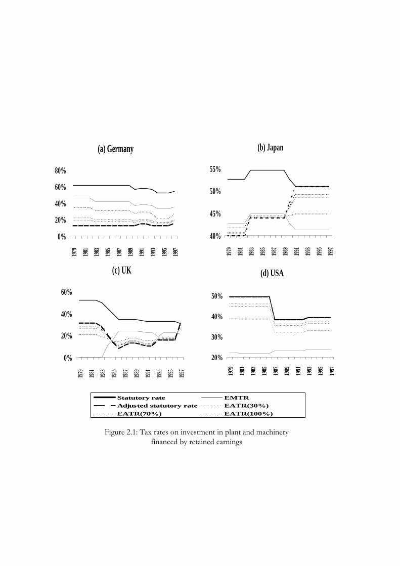
The four panels of Figure 2.1 each illustrate the development of the domestic

corporation tax system over the period 1979 to 1997 for each country. In each case, the

personal tax rates of the marginal investor are assumed to be zero. The tax rates shown

in each panel are: the statutory tax rate on retained earnings; the EMTR for domestic

investment in plant and machinery financed by retained earnings; the adjusted statutory

tax rate, ( )jτγ −− 11 , and values of the EATR, for the same investment for profitability

rates of 30%, 70% and 100%, p = 0.3, 0.7, 1.0.

Figure 2.1 illustrates several of the properties of the EATR discussed above. At lower

levels of profitability the EATR tends to follow a similar pattern to the EMTR, while at

higher levels of profitability it tends to follow a similar pattern to the adjusted statutory

tax rate. However, the relative magnitude of the EMTR and the adjusted statutory tax

rate varies both between countries and over time. In Germany, for example, the EMTR

is strongly correlated with the statutory tax rate, and is always higher than the adjusted

statutory tax rate, ( )jτγ −− 11 . Although the statutory tax rate in Germany has been

consistently high, Germany operated a system close to full integration throughout this

period and thus γ was also high, implying a very low value of ( )jτγ −− 11 . The opposite

is true of the USA, where the 1986 reforms had the effect of reducing the statutory tax

rate but increasing the EMTR. Since the USA operated a classical system over the whole

12 A more detailed descriptions of the tax systems in each of these countries is given in Chennells andGriffith (1997).

32

period, g = 1 in the absence of personal taxes, and so ( ) jj ττγ =−− 11 . Hence at low

rates of profit, the EATR increased following the 1986 reforms; but at high rates of

profit it fell.

This process was even more extreme in the UK, where the 1984 reforms reduced the

statutory tax rate in stages from 52% to 35%, but at the same time reduced depreciation

allowances, summarised here by A . The combination of these reforms led to an increase

in the EMTR, but a reduction in the adjusted statutory tax rate: in fact these two rates

crossed in 1984. As a consequence, before the 1984 reforms the EATR increased with

profitability; but after the 1984 reforms, the reverse was true. The 1997 reforms reduced

γ to 1.0 for tax-exempt shareholders, raising ( )jτγ −− 11 to the statutory tax rate, and

switching the sign of pEATR

∂∂ back again.

The position in Japan has various elements of those seen in the other countries. For

example, like Germany the EMTR is positively correlated with the statutory tax rate.

Also like Germany, in the first half of the period, the EMTR was above the adjusted

statutory tax rate, implying that the EATR was lower for higher rates of profit. However,

in 1991, γ fell from 1.27 to 1.0 for tax-exempt shareholders. Like the 1997 reform in the

UK this raised ( )jτγ −− 11 equal to t j and had the effect of switching the sign of

∂ ∂EATR p/ .

5.2 Alternative production technologies

One of the economic situations in which it was argued above that the EATR may affect

investment is in the choice between a number of alternative discrete methods of

production. If these alternative methods use different assets, or the same assets in

different proportions, then the EATR may affect firms’ choice between technologies. To

33

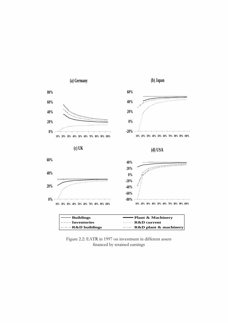
explore this, for each country using the 1997 tax system, the four panels of Figure 2.2

plot the EATR for domestic investment financed by retained earnings in six different

assets – industrial buildings, industrial plant and machinery, inventories, current R&D

expenditure, R&D buildings and R&D plant and machinery – against the rate of profit of

the investment, summarised by p. Tax systems in all four countries treat these assets

differently from each other by allowing different rates of depreciation and in some cases

by giving additional allowances or tax credits. Each line in the figure begins at the point

where the project is marginal – that is pp ~= and the EATR is equal to the EMTR.13

The most notable feature of Figure 2.2 is that in all countries, as profitability increases,

the EATR for investment in different assets converges to ( )jτγ −− 11 , which is

independent of tax depreciation rates and credits (summarised by A). The reason is clear:

as profitability increases, the value of depreciation allowances and other tax credits

becomes smaller relative to the tax on the return. That is, variations in A across assets

become less important. This suggests that studies which use the EMTR to examine the

distortions in production technology may exaggerate the differences in the relevant

effective tax rate faced by investors in these assets. In turn, this implies that estimates of

the impact of tax on asset choice using the EMTR rather than the EATR may

underestimate the true structural coefficients.

5.3 Choice of location of production

Another of the economic situations discussed above is the choice between alternative

locations for production. This issue is addressed empirically in Devereux and Griffith

13 For presentation reasons the line for R&D current expenditure for the USA does not start at the cost ofcapital, but at 10% profitability. This is because the EMTR for this investment is very large and negative.

34

(1998) and is illustrated here in two ways: by considering how the tax rate varies across

location choices facing a US-resident firm deciding where to locate production; and by

considering how it varies for foreign-resident firms investing in the USA. In calculating

the effective tax rates shown in Figures 2.3 and 2.4 the parent firm is assumed to be

financed by retained earnings but alternative forms of transfer between the parent and

the subsidiary are allowed.

5.3.1 Investment by US-resident firm

The first of these questions is examined in detail in Devereux and Griffith (1998) where a

firm level panel is used to estimate the impact of the EATR on the location decision of

US firms serving the European market. The empirical results indicate that the EATR

plays a direct and significant role in determining firms’ location choices.

The 4 panels of Figure 2.3 plot the EATR against the rate of profit of an investment in

1997. Panel (a) shows the position of a domestic firm undertaking investment in plant

and machinery financed by retained earnings. The other panels show the EATR faced by

a US parent investing in plant and machinery in each of the 4 countries, each for a

different form of financing of the foreign subsidiary (the line representing domestic

investment in the USA is the same in each of the 4 panels). As in Figure 2.2, each line

begins at the marginal investment, nn pp ~= .

Panel (a) shows the EATR for 1997, corresponding to Figure 2.1. The German domestic

EATR falls as the rate of profit increases, while the domestic EATR in the other three

countries increases with the rate of profit. Panel (b) shows the case of a subsidiary of a

US parent locating in each country financed by retained earnings. As noted in

Proposition 4 above, the EMTR in this case is independent of the overall tax rate

(including US tax) on dividends paid by the subsidiary to the parent, s jn . Hence, at the

35

margin for tax exempt shareholders of the parent firm, only source country taxes affect

the EMTR. However, this is in general not true for the EATR. Although the ranking of

the EATR across the four possible locations does not change as the rate of profit

increases, the differences between them do vary. For example, at a high rate of profit,

Japan has a substantially higher EATR than the other three countries, all of which are

close to each other. At the margin, however, the EATR in Japan is only marginally higher

than that in Germany, both of which are substantially higher than those in the UK and

USA.

Panels (c) and (d) investigate alternative methods of the parent financing the subsidiary,

by new equity and debt respectively, thereby introducing the Fn terms from (4.2) and

Table A.4. In most cases introducing these extra terms increases the EATR, indicating

that international investment financed by both new equity and debt is more heavily taxed

overall than investment financed by retained earnings. An exception to this is the case of

new equity investment into Germany, which benefits from the high level of γ applying to

US parents investing in Germany.14 Note though, that this benefit is greatest at low rates

of profit; this is because the benefit to new equity investment depends on the cost of the

investment, but not on the rate of profit earned. This implies again that the EMTR –

computed for a marginal investment - represents an extreme case in comparing

alternative forms of finance.

14 US parents do not receive the same integration tax credit as German resident shareholders; however,

they do benefit from the German split rate corporation tax, which, in effect, also generates a high value of

γ relative to other forms of investment.

36

5.3.2 Investment by foreign-resident firm

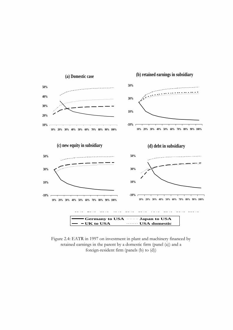
The panels in Figure 2.4 provide similar information to those in Figure 2.3 but show the

tax rate on investment into the USA by parent companies in each of the other countries.

For comparison, panel (a) repeats the position for domestic investment. In the other

panels, the parent firm is financed by retained earnings, and the EATR is again shown

separately for each of the three ways in which the subsidiary may be financed: retained

earnings in panel (b), new equity in panel (c), and debt in panel (d).

Panel (b) illustrates Proposition 4 from Section 3.4. The EMTR for international

investment financed by retained earnings depends only on source country taxation; this

implies that it is the same for investment by each of the foreign subsidiaries investing in

the USA, as well as for domestic firms. Since at this point the EMTR is equal to the

EATR, the position of all four potential investors is the same at this point. However, as

the expected rate of profit, pn, increases the EATRs vary by location of investor. In

particular, while the EATR for domestic investment and inward investment from Japan

and the UK increases with pn , the reverse is true for inward investment from Germany.

The position for Germany is due to the high value of γ, which under the circumstances

assumed here, implies that German shareholders can, in effect, claim back much of the

tax paid in the USA.15

Panels (c) and (d) reflect the additional tax costs and benefits from the Fn terms in Table

2.4. These panels provide a striking illustration of the differences across investors in the

EATR faced at different rates of profit. For example, for marginal investment financed

15 This requires the German parent to pay dividends out of domestic income for tax purposes, but in effect

financed from foreign source income. See Weichenreider (1996, 1997) for a fuller analysis of this

possibility.

37

by debt (panel (d)), Germany appears substantially disadvantaged relative to other

investors: this is because interest paid from the USA to Germany receives relief at the

relatively low US statutory tax rate, but is taxed at the relatively high German tax rate.

However, at higher rates of profit, the importance of this factor (which is unrelated to

the rate of profit) is outweighed by the benefit of the high γ in Germany, so that the

EATR for German investors in the USA becomes substantially lower than the EATRs

for other investors in the USA.

6 SUMMARY

This paper has investigated the role of taxation in cases in which an investor faces a

choice between two or more mutually exclusive projects that earn more than the

minimum required rate of return. It is argued that there are a number of circumstances in

which such a choice is likely to occur, including choice of location and choice of

technology. The choice of which project to undertake depends on the level of the post-

tax economic rent that would be earned from each option. The impact of taxation on the

choice cannot therefore be measured in the standard way by analysing a marginal

investment. Instead, the impact depends on the proportion of economic rent captured in

tax.

A new measure - an effective average tax rate (EATR) – is proposed, which attempts to

summarise the impact of tax in such choices, and which builds on the standard approach

to measuring the effective marginal tax rate (EMTR). This measure of the EATR has

several attractive properties including that, for a marginal investment, it is equal to the

EMTR. It can therefore be interpreted as summarising the distribution of tax rates for an

investment project over a range of profitability; the EMTR represents the special case of

a marginal investment. Estimates of the EATR are presented for four countries –

38

Germany, Japan, UK and USA - over the period 1979-1997. They illustrate several

features of the EATR.

REFERENCES

Alworth, J. (1988) The finance, investment and taxation decision of multinationals, Basil Blackwell: NewYork

Auerbach, A.J. (1979) “Wealth maximization and the cost of capital”, Quarterly Journal of Economics,21:107-127

Auerbach, A.J. (1983) “Corporate taxation in the United States,” Brookings Papers on EconomicActivity, 2: 451-505

Bloom, N., Chennells, L., Griffith, R. and Van Reenen, J. (1999) “How Has Tax Affected theChanging Cost of R&D? Evidence from Eight Countries” forthcoming in The Regulationof Science and Technology, H.L.Smith (ed.), Macmillan: London

Caves, R. (1996) Multinational Enterprise and Economic Analysis, 2nd edition, Cambridge, England:Cambridge University Press

Chennells, L. and Griffith, R. (1997) Taxing profits in a changing world, Institute for Fiscal Studies.Collins, J.H. and D.A. Shackelford (1995) “Corporate Domicile and Average Effective Tax Rates:

The Cases of Canada, Japan, the UK and USA”, International Tax and Public Finance, Vol 2,55-83.

Devereux, M.P. and R. Griffith (1998) “Taxes and the location of production: evidence from apanel of US multinationals”, Journal of Public Economics, 68(3), 335-367

Devereux, M.P., Keen, K.J. and F. Schiantarelli (1994) “Corporation tax asymmetries andinvestment: evidence from UK panel data", Journal of Public Economics, 53, 395-418

Dunning, J.H. (1977) “Trade, location of economic activity and MNE: a search for an eclecticapproach”, in B. Ohlin, P.O. Hesselborn and P.M. Wijkman eds. The InternationalAllocation of Economic Activity, London: Macmillan, 395-418.

Dunning, J.H. (1981) International Production and the Multinational Enterprise, London: George Allenand Unwin.

Edwards, J.S.S and M.J. Keen (1984) “Wealth maximization and the cost of capital: a comment”,Quarterly Journal of Economics, XCVIII, 211-214.

Fershtman, C., N. Gandal and S. Markovich “Estimating the effect of tax reform in differentiatedproduct oligopolistic markets” Tel Aviv University Working Paper No. 29-97

Goolsbee, A., “Taxes and the quality of capital”, University of Chicago and NBER mimeoGrubert, H. and J. Mutti (1996) “Do taxes influence where US multinational corporations

invest?” paper presented at TAPES conference, Amsterdam, 1996Hall. R.E. and D. Jorgensen (1967) “Tax policy and investment behavior”, American Economic

Review, 57, 391-414.Hartman D.G. (1985) “Tax policy and foreign direct investment”, Journal of Public Economics, 26,

107-121.Horstmann, I. and Markusen, J. (1992) “Endogenous market structures in international trade

(natura facit saltum)” Journal of International Economics, 32, 109-129Hubbard, R.G. (1998) “Capital-market imperfections and investment”, Journal of Economic

Literature, XXXVI, 193-225.Jorgensen, D.W. (1963) "Capital theory and investment behaviour", American Economic Review, 53,

247-59Judd, K. (1997) “Optimal taxation and spending in general competitive growth models”, Journal of

Public Economics (71)1 (1999) pp. 1-25Keen, M.J. (1991) “Corporation tax, foreign direct investment and the single market” in L.A.

Winters and AJ Venables (eds.) The Impact of 1992 on European Trade and Industry,Cambridge University Press: Cambridge

39

King. M.A. (1974) “Taxation, investment and the cost of capital”, Review of Economic Studies, 41,21-35.

King, M.A. and D. Fullerton (1984) The Taxation of Income from Capital, Chicago: University ofChicago Press.

Markusen, J. (1995) “The boundaries of multinational enterprises and the theory of internationaltrade”, Journal of Economic Perspectives, 9(2), 169-189.

OECD (1991) Taxing Profits in a Global Economy, Paris: OECD.Swenson, D. (1994) “The impact of US tax reform on foreign direct investment in the United

States”, Journal of Public Economics, 54, 243-266.Weichenreider, A. (1996), “Fighting international tax avoidance: the case of Germany”, Fiscal

Studies 17:1, 37-58Weichenreider, A. (1997) “Foreign profits and domestic investment”, Journal of Public

Economics

(a) Germany

0%

20%

40%

60%

80%

1979

1981

1983

1985

1987

1989

1991

1993

1995

1997

(b) Japan

40%

45%

50%

55%

1979

1981

1983

1985

1987

1989

1991

1993

1995

1997

(c) UK

0%

20%

40%

60%

1979

1981

1983

1985

1987

1989

1991

1993

1995

1997

(d) USA

20%

30%

40%

50%

1979

1981

1983

1985

1987

1989

1991

1993

1995

1997

Figure 2.1: Tax rates on investment in plant and machineryfinanced by retained earnings

1979

1981

1983

1985

1987

1989

1991

1993

1995

1997

Statutory rate EMTR

Adjusted statutory rate EATR(30%)

EATR(70%) EATR(100%)

(a) Germany

0%

20%

40%

60%

80%

10% 20% 30% 40% 50% 60% 70% 80% 90% 100%

(b) Japan

-20%

0%

20%

40%

60%

10% 20% 30% 40% 50% 60% 70% 80% 90% 100%

(c) UK

0%

20%

40%

60%

10% 20% 30% 40% 50% 60% 70% 80% 90% 100%

(d) USA

-80%-60%

-40%-20%

0%

20%40%

10% 20% 30% 40% 50% 60% 70% 80% 90% 100%

Figure 2.2: EATR in 1997 on investment in different assetsfinanced by retained earnings

Buildings Plant & MachineryInventories R&D currentR&D buildings R&D plant & machinery

(a) Domestic case

10%

20%

30%

40%

50%

10% 20% 30% 40% 50% 60% 70% 80% 90% 100%

(b) retained earnings in subsidiary

20%

30%

40%

50%

60%

10% 20% 30% 40% 50% 60% 70% 80% 90% 100%

(c) new equity in subsidiary

0%

20%

40%

60%

10% 20% 30% 40% 50% 60% 70% 80% 90% 100%

(d) debt in subsidiary

-10%

10%

30%

50%

10% 20% 30% 40% 50% 60% 70% 80% 90% 100%

Figure 2.3: EATR in 1997 on investment in plant and machinery financed byretained earnings in the parent by a domestic firm (panel (a)) and a

US-resident firm (panels (b) to (d))

in Germany in Japan in UK Domestic

(a) Domestic case

10%

20%

30%

40%

50%

10% 20% 30% 40% 50% 60% 70% 80% 90% 100%

(b) retained earnings in subsidiary

-10%

10%

30%

50%

10% 20% 30% 40% 50% 60% 70% 80% 90% 100%

(c) new equity in subsidiary

-10%

10%

30%

50%

10% 20% 30% 40% 50% 60% 70% 80% 90% 100%

(d) debt in subsidiary

-10%

10%

30%

50%

10% 20% 30% 40% 50% 60% 70% 80% 90% 100%

10% 20% 30% 40% 50% 60% 70% 80% 90% 100%

Germany to USA Japan to USAUK to USA USA domestic

Figure 2.4: EATR in 1997 on investment in plant and machinery financed byretained earnings in the parent by a domestic firm (panel (a)) and a

foreign-resident firm (panels (b) to (d))

40

APPENDIX A: FORMAL MODEL OF INTERNATIONAL

INVESTMENT

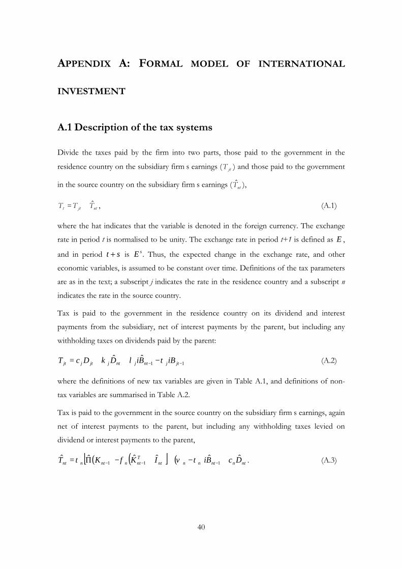
A.1 Description of the tax systems

Divide the taxes paid by the firm into two parts, those paid to the government in the

residence country on the subsidiary firm’s earnings (T jt ) and those paid to the government

in the source country on the subsidiary firm’s earnings ( $Tnt ),

T T Tt jt nt= + $ , (A.1)

where the hat indicates that the variable is denoted in the foreign currency. The exchange

rate in period t is normalised to be unity. The exchange rate in period t+1 is defined as E ,

and in period t s+ is E s . Thus, the expected change in the exchange rate, and other

economic variables, is assumed to be constant over time. Definitions of the tax parameters

are as in the text; a subscript j indicates the rate in the residence country and a subscript n

indicates the rate in the source country.

Tax is paid to the government in the residence country on its dividend and interest

payments from the subsidiary, net of interest payments by the parent, but including any

withholding taxes on dividends paid by the parent:

11ˆˆ

−− −++= jtjntjntjjtjjt iBBiDDcT τλκ (A.2)

where the definitions of new tax variables are given in Table A.1, and definitions of non-

tax variables are summarised in Table A.2.

Tax is paid to the government in the source country on the subsidiary firm’s earnings, again

net of interest payments to the parent, but including any withholding taxes levied on

dividend or interest payments to the parent,

( ) ( )[ ] ( ) ntnntnnntTntnntnnt DcBiIKKT ˆˆˆˆˆˆ

111 +−++−Π= −−− τϖφτ . (A.3)

41

Table A.1: Tax parameters

Taxation of dividend paymentsc cj n, withholding tax rate on gross dividends paid by the parent (j) and by the subsidiary (n)

s j imputation credit on dividends received by the ultimate shareholder from the parent

c sj j= classical system

c sj j< partial imputation system

c sj j> net withholding tax

κ j residence country tax rate on dividends received by the parent from the subsidiary

= 0 Exemption

=

−

−

−0,

1max n

n

nj cτ

ττ partial credit with deferral

= ( )nj c−1τ deduction with deferral

σ jn overall tax rate on dividend payments from the subsidiary to the parent

= nc Exemption

=

−

−n

n

nj c,1

maxτ

ττ partial credit with deferral

= ( ) nnj cc +−1τ deduction with deferral

Taxation of interest paymentsϖ n

withholding tax rate on interest payments made by the subsidiary (n) to the parent

λ j residence country tax rate on interest payments received by the parent from the subsidiary

= 0 Exemption

= ( ){ }0,max nj ϖτ − partial credit with deferral

= ( )nj ϖτ −1 Deduction with deferral

ω jn overall tax rate on interest payments from the subsidiary to the parent

=ϖ τn n− Exemption

= { } nnj τϖτ −,max partial credit with deferral

= ( ) nnnj τϖϖτ −+−1 deduction with deferral

42

Table A.2: Definition of non-tax variables

i nominal interest rate in the presence of tax

tV net present value of the firm to the ultimate shareholder in period t

N Njt nt, $ new equity issued by the parent (j) and issued by the subsidiary to the parent (n) in period t

D Djt nt, $ Dividends paid by the parent to the ultimate shareholder (j) and from the subsidiary to theparent (n) in period t gross of withholding tax at the firm level, but before imputation credit atthe shareholder level

nΠ net income of subsidiary (n)

1ˆ

−ntK the value of the capital stock at the end of period t-1, beginning of period t of subsidiary (n)

ntI Investment made in period t of subsidiary (n)

B Bjt nt, $ one-period debt borrowed by the parent (j), and borrowed by the subsidiary from the parent (n)in period t

δ Economic depreciation rateρ ultimate share holder’s discount rate

π πj n, expected inflation in the parent (j) and subsidiary (n) country

E expected exchange rate in period t+1, E Et ss

+ =∧ denotes a variable in the currency of the source (n) country

An allowance is given on investment at the end of the first and subsequent periods. If the

allowance is given on a declining balance basis the equation of motion of the tax written

down value of the subsidiary’s capital stocks is:

( ){ }ntTntn

Tnt IKK ˆˆ1ˆ

1 +−= −φ . (A.4)

Combining (A.2) and (A.3) gives a general expression for total corporate level taxes paid in

period t:

( ) [ ] jtjntjnntjnjtjntTntnnntnj DcDBiiBIKKT +++−+−Π= −−−−

ˆˆˆˆˆ1111 σωτφττ . (A.5)

A.2 The model

Consider a value-maximising parent firm. As in the main text, the value of the firm can be

derived from the capital market equilibrium condition as,

( ) jttjtt NVDV −+=− +11 γρ (A.6)

where the tax discrimination term is here defined as ( )( )( )( )jj

jdj

sz

cm

−−

−−=

11

11γ . As in the

domestic case, an expression for the value of D jt must be derived, which incorporates the

43

activities of both the parent firm and the subsidiary. Using the equality of sources and uses

of funds in the parent, dividends paid by the parent, D jt , are given by

( ) ( )( )[ ] ( ) ntnntnntnt

jtjtjtjtjtj

DcBiNB

TNBiBDc

ˆ1ˆ11ˆˆ

11

1

1

−+−++−−

−+−−=−

−

−

ϖ (A.7)

Note that the parent is assumed to raise all its finance in the residence country j. The

equivalent expression for dividends paid by the subsidiary to the parent, $Dnt , is,

( ) ( ) ( )[ ] ntntntntnntntntn TINBiBKDc ˆˆˆˆ11ˆˆˆ1 11 −−+−+−+Π=− −− ϖ . (A.8)

The subsidiary raises all its finance from the parent; it does not issue either debt or equity

in the source country. As for the domestic case, we simplify the analysis by assuming that

there is no specific price change for capital goods relative to output; we choose units such

that the price of output is equal to the price of capital goods, and normalise this to be unity

in period t. In period t+1 the price in the foreign currency is ( )nπ+1 . Combining, (A.7),

(A.8), (A.2) and (A.3) and rearranging gives a general expression for dividends paid by the

parent,

( )( ) ( ) ( )[ ]( )( )[ ]

( )( ) ( ) Tntnnjnntnnjn

ntjnnjnntjn

jtjjtntjnjtntnjnjt

KI

BiiB

BiBNNKD

1

1

11

ˆ1ˆ11

ˆ11ˆ

11ˆˆ11

−

−

−−

−+−−−

−−++−

−+−+−+Π−−=

φτσφτσ

ωτσσ

τστσ

(A.9)

The equations of motion of the value of the capital stock is given by

( )( ) ntntnnt IKK ˆˆ11ˆ1 ++−= −πδ . (A.10)

The net present value of the tax depreciation allowances per unit of investment, nA , where

depreciation is given on a declining balance basis was given in equation (3.6) for the

domestic case. Where tax depreciation is allowed at rate nφ on a straight line basis it is

given by,

( )( )

+−

−++

=N

n

N

n

nnnn

E

EA

ρρρτφ

11

1

1. (A.11)

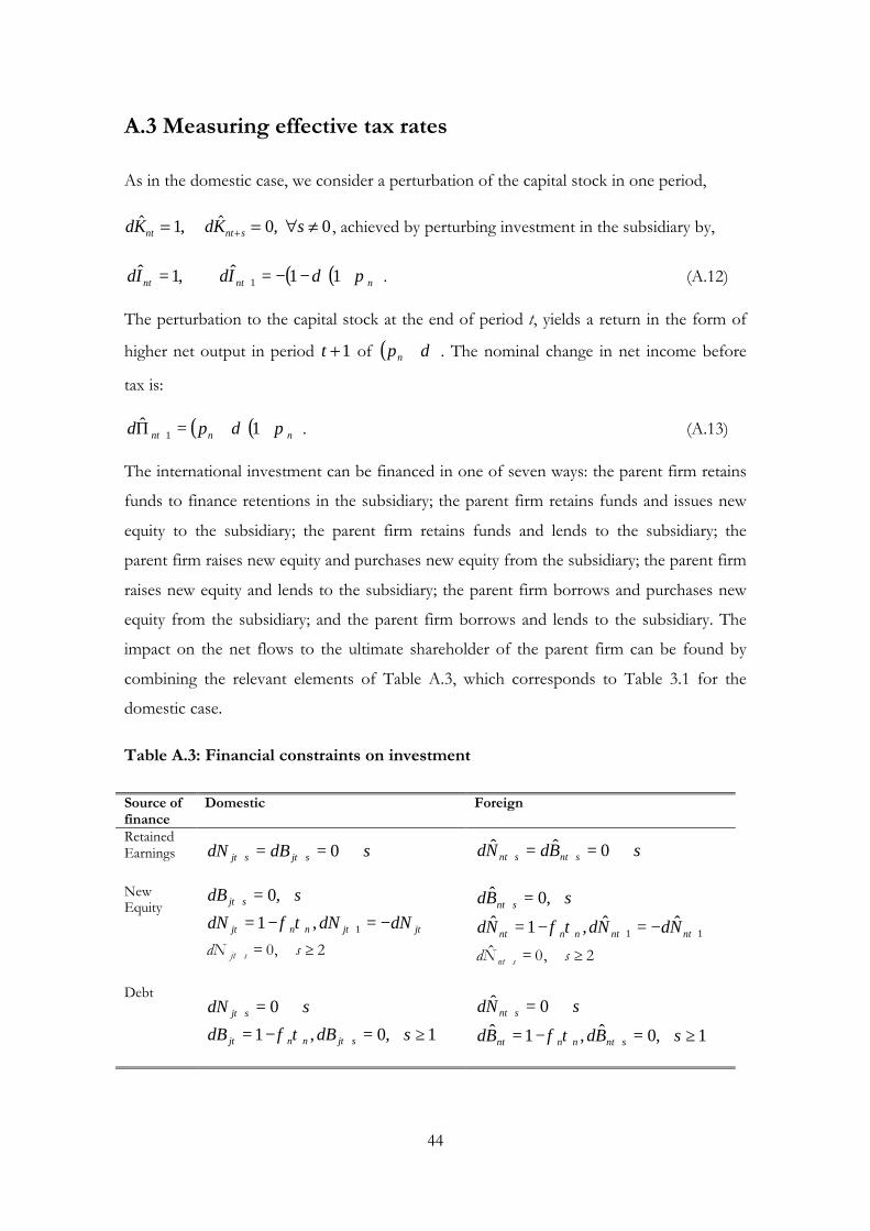
44

A.3 Measuring effective tax rates

As in the domestic case, we consider a perturbation of the capital stock in one period,

dK dK snt nt s$ , $ ,= = " π+1 0 0 , achieved by perturbing investment in the subsidiary by,

( )( )nntnt IdId πδ +−−== + 11ˆ,1ˆ1 . (A.12)

The perturbation to the capital stock at the end of period t, yields a return in the form of

higher net output in period t +1 of ( )δ+np . The nominal change in net income before

tax is:

( )( )nnnt pd πδ ++=Π + 1ˆ1 . (A.13)

The international investment can be financed in one of seven ways: the parent firm retains

funds to finance retentions in the subsidiary; the parent firm retains funds and issues new

equity to the subsidiary; the parent firm retains funds and lends to the subsidiary; the

parent firm raises new equity and purchases new equity from the subsidiary; the parent firm

raises new equity and lends to the subsidiary; the parent firm borrows and purchases new

equity from the subsidiary; and the parent firm borrows and lends to the subsidiary. The

impact on the net flows to the ultimate shareholder of the parent firm can be found by

combining the relevant elements of Table A.3, which corresponds to Table 3.1 for the

domestic case.

Table A.3: Financial constraints on investment

Source offinance

Domestic Foreign

RetainedEarnings sdBdN sjtsjt ∀== ++ 0 sBdNd sntsnt ∀== ++ 0ˆˆ

NewEquity

sdB sjt ∀=+ ,0

jtjtnnjt dNdNdN −=−= +1,1 τφdN sjt s+ = ∀ ≥0 2,

sBd snt ∀=+ ,0ˆ

11ˆˆ,1ˆ

++ −=−= ntntnnnt NdNdNd τφ

dN snt s$ ,+ = ∀ ≥0 2

DebtsdN sjt ∀=+ 0

1,0,1 ≥∀=−= + sdBdB sjtnnjt τφ

sNd snt ∀=+ 0ˆ

1,0ˆ,1ˆ ≥∀=−= + sBdBd sntnnnt τφ

45

The economic rent of the new project, defined as R , is the net present value of the change

in the value of the firm, and is identical to (3.8). As in the domestic case, we implement this

definition by deriving the change in dividends and new equity in each period. This can be

usefully split into three parts (we drop time subscripts for expositional purposes): (i) the

rent attributable to the investment in the subsidiary financed by retained earnings ( REnR );

(ii) the additional cost of the parent raising external finance ( F j ); and (iii) the additional

cost of the subsidiary of raising finance from the parent ( Fn ). The economic rent earned

from an investment by the subsidiary is given by njREnn FFRR ++= . RE

nR is defined in

(4.1), jF in (3.10) and nF in (4.2). The values of Fj

Fn

, are given in Table A.4 for the

different sources of finance.

Table A.4: Values of Fj

Fn

, for alternative forms of investment

Source of parent financeRetained Earnings 0=jFNew Equity ( )

( ) ( )nnjF τφρ

γρ−

+−−

= 11

1

Debt ( )( ) ( ){ }j

nnj iF τρ

ρτφγ

−−+

−= 1

1

1

Source of subsidiary financeRetained Earnings 0=nFNew Equity

( ) ( ) ( )[ ]ρτφρ

γσ+−−

+= 11

1EF nn

jnn

Debt ( )( ) ( )( ) ( )[ ]{ }iEiEF jnnjn

nnn ωρτσ

ρτφγ

−+−−++

−= 111

1

1

Setting 0=R and solving for np , the cost of capital for an international investment,

defined as np~ , yields equation (4.3).

The EATR is defined in equation (4.5). Substituting for *nR from (4.4) and for nR using

the expressions for REnR from (4.1) permits the EATR to be derived for a given value of

np :

46

( )

( )( ) ( )( )

( )

( )( ) ( ) ( )( ) ( ) ( )( )[ ]( ){ }

( )

( )

+++

−

++

−+−−+−−+++

−

−

++

++−++

=

++

−=

i

pE

FF

i

pE

AEp

i

pEi

ipE

i

pE

RREATR

nn

nj

nn

nnnnnnjn

nn

nn

nn

nnn

1

1

1

1

1111111

1

1

11

111

1

1

*

π

π

πδρτπδρ

σγ

π

π

π

(A.14)

This can be computed for different forms of finance and hence different values of jF and

nF using the expression in Table A.4. The corresponding general expression for the EATR

of a domestic investment is,

( ) ( )( )( ) ( ) ( )( )[ ]( ){ }.

1

1111111

1

1

1

*

+

+−+−−+−−+++−

+

+−

=

+

−=

r

p

FAp

r

pr

rp

r

p

RREATR

jjjjj

jjj

πδρτπδρ

γ (A.15)

47

APPENDIX B: TAX DATA

The information on corporate tax systems comes largely from Chennells and Griffith

(1997) and on the tax treatment of R&D from Bloom, Chennells, Griffith and Van Reenen

(1999).

Statutory tax rates

Three statutory tax rates are shown below: the headline rate, and two statutory tax rates -

one applying to retained earnings, and the other to distributed profits - which include all

other taxes on corporate income. The headline rate is the national corporate income tax

rate on retained earnings. This rate does not include any surcharges or local taxes. The

statutory tax rates on retained earnings and distributed profits are the ones used in the

calculations presented and include surcharges and other special taxes that are levied on

corporate income at the national level. They also include an estimate of corporate income

tax levied at the local level. Local taxes only include local corporate income taxes, they do

not include taxes on property. In many countries local taxes are deductible from the

national tax and this is taken into account. The tax rates are based on the rates in force at

31 December.

Depreciation Allowances

Where there are several alternatives for the firm to choose from, the most generous form

of capital allowance is used. Where a switch from declining balance to straight line is

allowed it is assumed that this is made as soon as the value of the straight line depreciation

exceeds that of the declining balance. Where the depreciation rate is based on the life-time

of the asset, it is assumed that plant and machinery lasts for 8 years and buildings for 25

years. None of the countries considered here indexes allowances for inflation. In the

calculations shown in this appendix a fixed nominal discount rate of 10% has been used for

illustrative purposes.

For illustrative purposes, the measure of the net present value (NPV) of allowances given

in the tables below are calculated using equations (3.6) and (A.11) generalised to allow for

48

time-varying depreciation rates.1 The number reported is At so that a value of unity

indicates that the full cost of the investment can be offset immediately.

Structure of Tax Systems

There are some elements of tax systems which remain relatively unchanged over time,

including the treatment of inventories, the method of integrating corporate and personal

taxation for the treatment of dividend income, and the treatment of foreign source income.

The method by which firms are allowed to value inventories will affect their profit rate

(and therefore tax rate) in the presence of inflation. There are at least two commonly used

methods, FIFO (first in, first out) and LIFO (last in, last out). During periods of high

inflation, FIFO will value profits higher than LIFO and thus increase the effective tax rate.

In many countries firms can choose which method they want to use. Firms may want to

use FIFO to increase reported profits (particularly in one book countries), while for tax

reasons they would prefer to use LIFO. It is assumed that firms use LIFO unless this is

explicitly disallowed. Table B.1 shows the systems used in each of the five countries.

Table B.1: Valuation Method for Inventories

France FIFOGermany LIFOJapan LIFOUK FIFOUSA LIFO

Income from corporate profits can be the subject of taxation at two levels, the corporate

level and the personal income tax level. There are a variety of approaches that countries

have adopted to try and alleviate this “double” taxation through the integration of the

personal and corporate income tax systems. Table B.2. summarises these approaches into

one of three categories: split rate systems, imputation systems, and classical systems. Under

a split rate system there are two different statutory tax rates, one that applies to retained

earnings, the other to distributed earnings. The lower rate on distributed profits acts to

compensate, usually only partially, for the personal income tax levied on the dividend

income. An imputation system is one in which some portion of corporate income taxes

1 See OECD (1991).

49

paid on distributed profits can be offset against the individual personal income tax liability.

Under some systems this comes in the form of a credit which can be refunded if, for

example, the individual is tax-exempt. The rates of imputation given below are expressed as

a share of the gross dividend (i.e. the cash dividend plus its associated tax credit). A

classical system makes no allowance for “double” taxation, so that dividend income is

subject to corporate income tax and taxed again as personal income.

Table B.2: Method of Integrating Corporate and Personal Income Taxes

France Partial imputation system which gives shareholders a credit of 33% (called the avoir fiscal).Germany Germany operates a split rate system and an imputation system, the credit is 36% until 1994

when it drops to 30%.Japan Split rate system until 1990, partial shareholder relief system thereafter.

UK Imputation system, the credit is 30% until 1985, 29% in 1986, 27% in 1987, 25% from 1988to 1992 and 20% from 1993.

USA Classical system.

The treatment of repatriated income from foreign sources, in the form of dividend or

interest income, will affect the tax rates on international investments. The systems in place

in these five countries are shown in Table B.3.

Table B.3: Treatment of Foreign Source Income

Interest DividendsFrance Credit Exempt (95%)

Germany Credit ExemptJapan Credit Credit

UK Credit CreditUSA Credit Credit

The most common methods of dealing with foreign income are the credit method and the

exemption method. The former grants a credit for foreign taxes paid by the subsidiary

against the tax which would have been owed on that income by the parent had the

investment been wholly domestic. The credit method has several variations, according to

whether foreign source income is considered on a country by country basis or a world-wide

basis, or according to different classes of income. However, only investments into a single

country are considered here so these are effectively the same. The exemption method

exempts foreign income in the hands of the parent, so that the tax paid in the country

which is the source of the profits, the withholding tax paid when the subsidiary transfers

the income to the parent, and personal taxes owed by investors in the parent company are

the only taxes levied. One other alternative modelled here is a deduction system, which

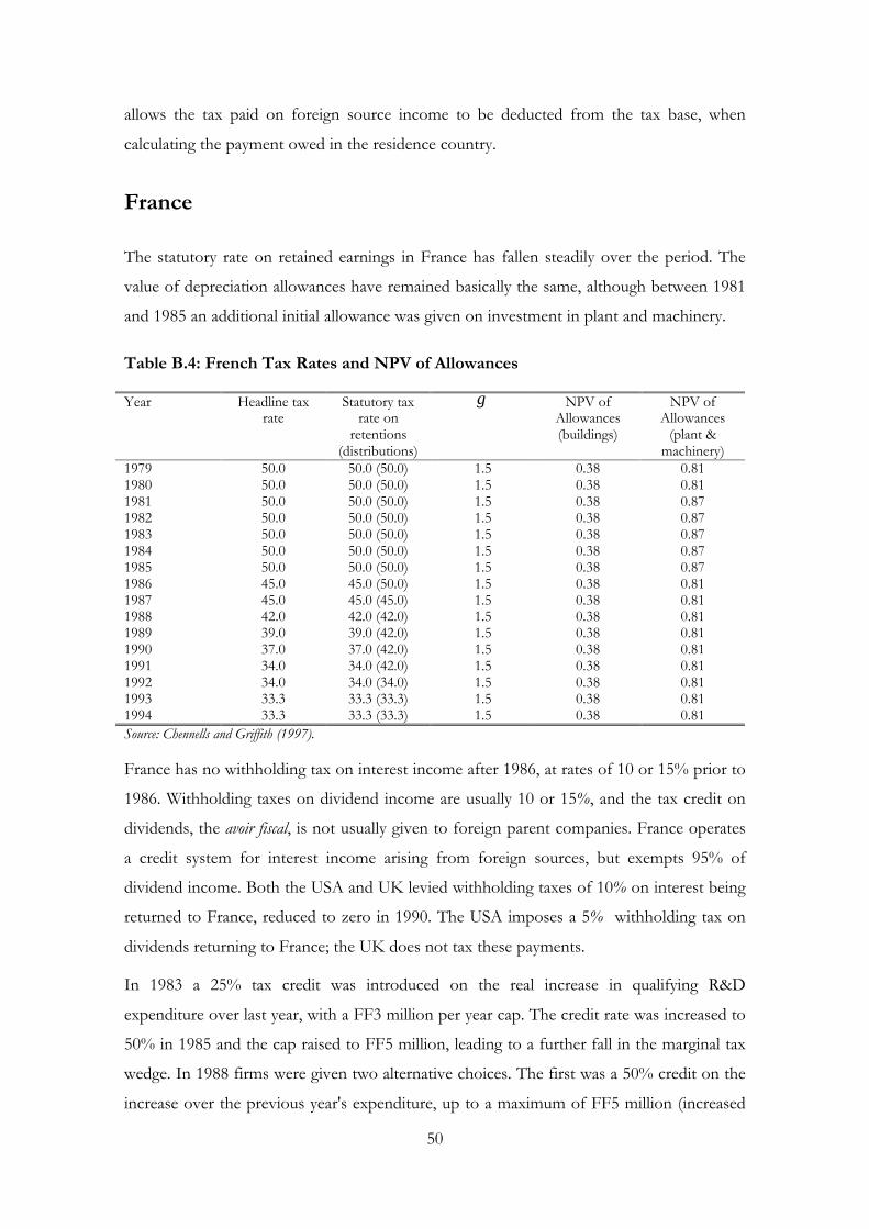
50

allows the tax paid on foreign source income to be deducted from the tax base, when

calculating the payment owed in the residence country.

France

The statutory rate on retained earnings in France has fallen steadily over the period. The

value of depreciation allowances have remained basically the same, although between 1981

and 1985 an additional initial allowance was given on investment in plant and machinery.

Table B.4: French Tax Rates and NPV of Allowances

Year Headline taxrate

Statutory taxrate on

retentions(distributions)

g NPV ofAllowances(buildings)

NPV ofAllowances

(plant &machinery)

1979 50.0 50.0 (50.0) 1.5 0.38 0.811980 50.0 50.0 (50.0) 1.5 0.38 0.811981 50.0 50.0 (50.0) 1.5 0.38 0.871982 50.0 50.0 (50.0) 1.5 0.38 0.871983 50.0 50.0 (50.0) 1.5 0.38 0.871984 50.0 50.0 (50.0) 1.5 0.38 0.871985 50.0 50.0 (50.0) 1.5 0.38 0.871986 45.0 45.0 (50.0) 1.5 0.38 0.811987 45.0 45.0 (45.0) 1.5 0.38 0.811988 42.0 42.0 (42.0) 1.5 0.38 0.811989 39.0 39.0 (42.0) 1.5 0.38 0.811990 37.0 37.0 (42.0) 1.5 0.38 0.811991 34.0 34.0 (42.0) 1.5 0.38 0.811992 34.0 34.0 (34.0) 1.5 0.38 0.811993 33.3 33.3 (33.3) 1.5 0.38 0.811994 33.3 33.3 (33.3) 1.5 0.38 0.81Source: Chennells and Griffith (1997).

France has no withholding tax on interest income after 1986, at rates of 10 or 15% prior to

1986. Withholding taxes on dividend income are usually 10 or 15%, and the tax credit on

dividends, the avoir fiscal, is not usually given to foreign parent companies. France operates

a credit system for interest income arising from foreign sources, but exempts 95% of

dividend income. Both the USA and UK levied withholding taxes of 10% on interest being

returned to France, reduced to zero in 1990. The USA imposes a 5% withholding tax on

dividends returning to France; the UK does not tax these payments.

In 1983 a 25% tax credit was introduced on the real increase in qualifying R&D

expenditure over last year, with a FF3 million per year cap. The credit rate was increased to

50% in 1985 and the cap raised to FF5 million, leading to a further fall in the marginal tax

wedge. In 1988 firms were given two alternative choices. The first was a 50% credit on the

increase over the previous year's expenditure, up to a maximum of FF5 million (increased

51

to FF10 million in certain cases). Alternatively, for the years 1988, 1989, and 1990 they

could receive a 30% credit on the increase over their 1987 expenditure, up to a maximum

of FF3 million. This latter option is worth more to firms expecting to increase their R&D

spending and is what is modelled. Although the headline rate of credit fell (from 50% to

30%), the value of the effective subsidy to R&D increased sharply because the base used to

calculate the increase in R&D expenditure was fixed at the 1987 level. This eliminates the

impact of current R&D spending on the calculation of the future base. In 1991 the credit

returned to 50% on the increase in real expenditure, but the base was extended to the most

recent two years and the cap raised to FF40 million. This reduced the effective value of the

subsidy due, since the base reverted to a moving average. From 1983 to 1986 expenditure

on buildings used for scientific research was given an accelerated depreciation allowance of

50% straight line.

Germany

Throughout most of the period, the German statutory tax rate has been the highest of the

countries considered here, although a significant decrease in 1994 meant that it fell slightly

below Japan. However, a surcharge reintroduced in 1995 increases the rate again. Germany

operates a split rate system with the statutory rate on distributed profits set significantly

lower than that on retained earnings. There have been two reductions in the statutory rate,

one in 1990 and the other in 1994. Depreciation allowances on buildings have become

more generous over time, while on plant and machinery they have increased only slightly.

52

Table B.5: German Tax Rates and NPV of Allowances

Year Headline Rate Statutory taxrate on

retentions(distributions)

γ NPV ofAllowances(buildings)

NPV ofAllowances

(plant &machinery)

1979 56.0 61.8 (44.4) 2.27 0.26 0.761980 56.0 61.8 (44.4) 2.27 0.26 0.761981 56.0 61.8 (44.4) 2.27 0.26 0.761982 56.0 61.8 (44.4) 2.27 0.26 0.761983 56.0 61.8 (44.4) 2.27 0.32 0.801984 56.0 61.8 (44.4) 2.27 0.32 0.801985 56.0 61.8 (44.4) 2.27 0.49 0.801986 56.0 61.8 (44.4) 2.27 0.49 0.801987 56.0 61.8 (44.4) 2.27 0.49 0.801988 56.0 61.8 (44.4) 2.27 0.49 0.801989 56.0 61.8 (44.4) 2.27 0.49 0.801990 50.0 56.6 (44.4) 2.00 0.49 0.801991 50.0 58.2 (45.6) 2.03 0.49 0.801992 50.0 58.2 (45.6) 2.03 0.49 0.801993 50.0 56.6 (44.4) 2.00 0.49 0.801994 45.0 52.2 (39.2) 1.82 0.49 0.801995 45.0 52.2 (39.2) 1.82 0.49 0.801996 45.0 52.2 (39.2) 1.82 0.49 0.801997 45.0 54.7 (41.0) 1.87 0.80Notes: The statutory rate on retained earnings and (distributed profits) includes local taxes and a ‘Solidarity’ Surcharge of3.75% on individual and corporation tax for 1991 and 1992, a surcharge on corporate income tax only of 7.5% wasintroduced in 1995. A local municipal trade tax is levied at a rate varying from 9 to 20%. A rate of 13.1% is assumedthroughout the period based on OECD 1991. The trade tax is deductible.Source: Chennells and Griffith (1997).

France, Japan and the US operate credit systems for the treatment of income from

Germany. Germany exempts interest income returned to these countries, but levies

withholding taxes on dividends at various rates, falling from 25% in 1979 to between 5 and

15% by 1994. Germany gives a credit for taxes paid on interest income earned abroad, and

exempts dividend income. Although the USA levies a withholding tax of 5% on dividends

being returned to Germany (15% prior to 1992), it does not impose a withholding tax on

interest. Neither the UK nor France withholds tax on dividend or interest payments made

to Germany.2

There are currently no special tax allowances for R&D in Germany. Between 1983 and

1989 industrial buildings and plant and machinery enjoyed limited accelerated depreciation

provisions. A building that was at least two-thirds used for R&D purposes could be

depreciated at up to 15% of the cost over five years; or 10% if only one-third used for

2 However, unlike its treatment of many European countries, the UK does not grant the dividend tax credit

for dividends remitted to Germany.

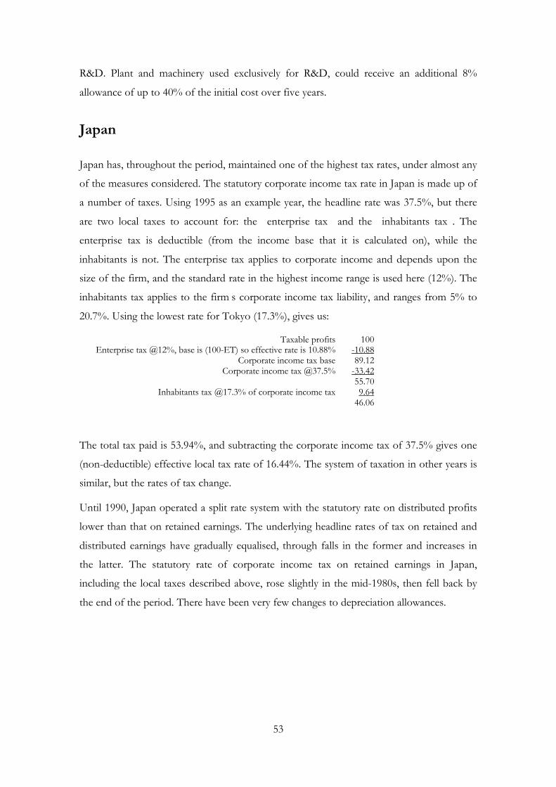
53

R&D. Plant and machinery used exclusively for R&D, could receive an additional 8%

allowance of up to 40% of the initial cost over five years.

Japan

Japan has, throughout the period, maintained one of the highest tax rates, under almost any

of the measures considered. The statutory corporate income tax rate in Japan is made up of

a number of taxes. Using 1995 as an example year, the headline rate was 37.5%, but there

are two local taxes to account for: the “enterprise tax” and the “inhabitants tax”. The

enterprise tax is deductible (from the income base that it is calculated on), while the

inhabitants is not. The enterprise tax applies to corporate income and depends upon the

size of the firm, and the standard rate in the highest income range is used here (12%). The

inhabitants tax applies to the firm’s corporate income tax liability, and ranges from 5% to

20.7%. Using the lowest rate for Tokyo (17.3%), gives us:

Taxable profits 100Enterprise tax @12%, base is (100-ET) so effective rate is 10.88% -10.88

Corporate income tax base 89.12Corporate income tax @37.5% -33.42

55.70Inhabitants tax @17.3% of corporate income tax 9.64

46.06

The total tax paid is 53.94%, and subtracting the corporate income tax of 37.5% gives one

(non-deductible) effective local tax rate of 16.44%. The system of taxation in other years is

similar, but the rates of tax change.

Until 1990, Japan operated a split rate system with the statutory rate on distributed profits

lower than that on retained earnings. The underlying headline rates of tax on retained and

distributed earnings have gradually equalised, through falls in the former and increases in

the latter. The statutory rate of corporate income tax on retained earnings in Japan,

including the local taxes described above, rose slightly in the mid-1980s, then fell back by

the end of the period. There have been very few changes to depreciation allowances.

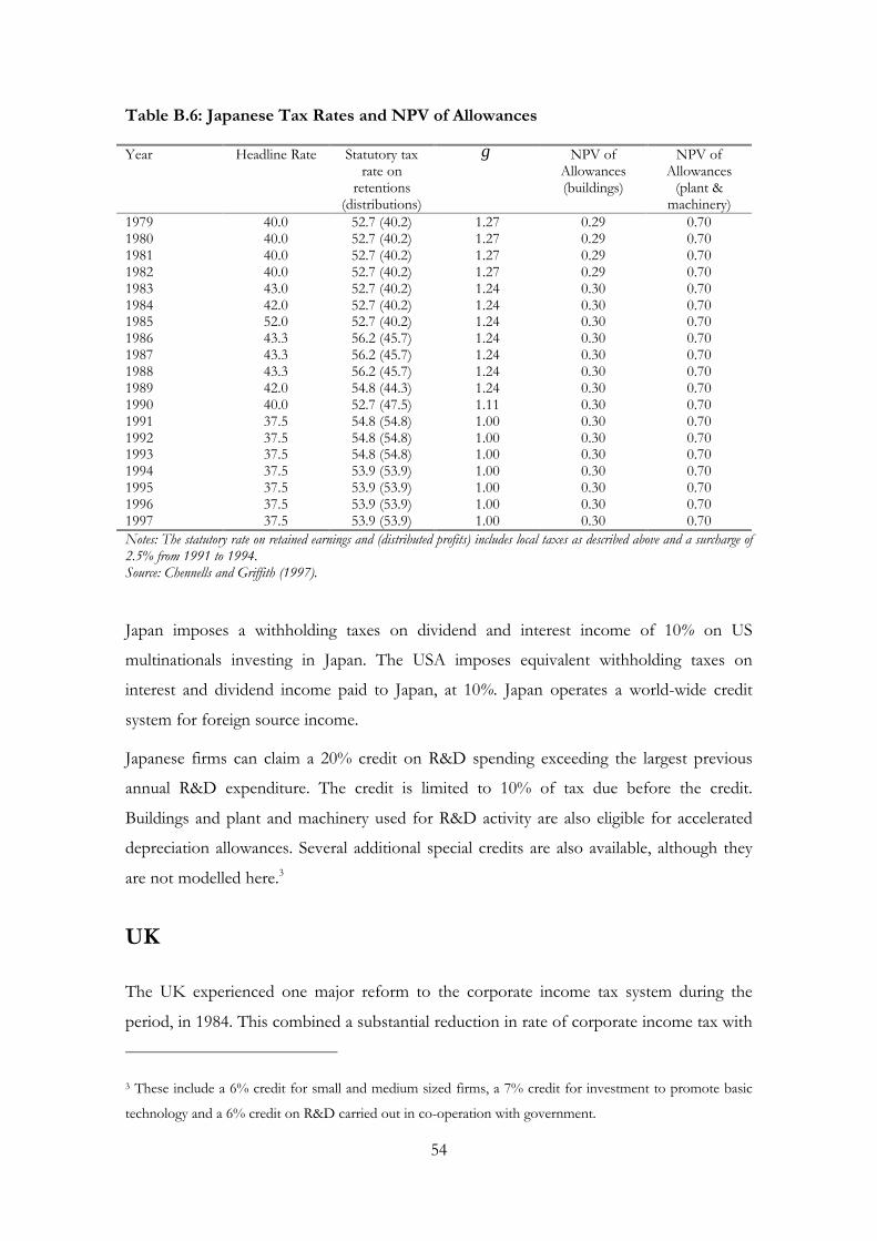
54

Table B.6: Japanese Tax Rates and NPV of Allowances

Year Headline Rate Statutory taxrate on

retentions(distributions)

γ NPV ofAllowances(buildings)

NPV ofAllowances

(plant &machinery)

1979 40.0 52.7 (40.2) 1.27 0.29 0.701980 40.0 52.7 (40.2) 1.27 0.29 0.701981 40.0 52.7 (40.2) 1.27 0.29 0.701982 40.0 52.7 (40.2) 1.27 0.29 0.701983 43.0 52.7 (40.2) 1.24 0.30 0.701984 42.0 52.7 (40.2) 1.24 0.30 0.701985 52.0 52.7 (40.2) 1.24 0.30 0.701986 43.3 56.2 (45.7) 1.24 0.30 0.701987 43.3 56.2 (45.7) 1.24 0.30 0.701988 43.3 56.2 (45.7) 1.24 0.30 0.701989 42.0 54.8 (44.3) 1.24 0.30 0.701990 40.0 52.7 (47.5) 1.11 0.30 0.701991 37.5 54.8 (54.8) 1.00 0.30 0.701992 37.5 54.8 (54.8) 1.00 0.30 0.701993 37.5 54.8 (54.8) 1.00 0.30 0.701994 37.5 53.9 (53.9) 1.00 0.30 0.701995 37.5 53.9 (53.9) 1.00 0.30 0.701996 37.5 53.9 (53.9) 1.00 0.30 0.701997 37.5 53.9 (53.9) 1.00 0.30 0.70Notes: The statutory rate on retained earnings and (distributed profits) includes local taxes as described above and a surcharge of2.5% from 1991 to 1994.Source: Chennells and Griffith (1997).

Japan imposes a withholding taxes on dividend and interest income of 10% on US

multinationals investing in Japan. The USA imposes equivalent withholding taxes on

interest and dividend income paid to Japan, at 10%. Japan operates a world-wide credit

system for foreign source income.

Japanese firms can claim a 20% credit on R&D spending exceeding the largest previous

annual R&D expenditure. The credit is limited to 10% of tax due before the credit.

Buildings and plant and machinery used for R&D activity are also eligible for accelerated

depreciation allowances. Several additional special credits are also available, although they

are not modelled here.3

UK

The UK experienced one major reform to the corporate income tax system during the

period, in 1984. This combined a substantial reduction in rate of corporate income tax with

3 These include a 6% credit for small and medium sized firms, a 7% credit for investment to promote basic

technology and a 6% credit on R&D carried out in co-operation with government.

55

reductions in the allowances available on plant and machinery and buildings, in a move

away from an expenditure-based tax.4

Table B.7: UK Tax Rates and NPV of Allowances

Year Headline Rate Statutory taxrate on

retentions(distributions)

γ NPV ofAllowances(buildings)

NPV ofAllowances

(plant &machinery)

1979 52.0 52.0 (52.0) 1.43 0.73 1.001980 52.0 52.0 (52.0) 1.43 0.73 1.001981 52.0 52.0 (52.0) 1.43 0.91 1.001982 52.0 52.0 (52.0) 1.43 0.91 1.001983 50.0 50.0 (50.0) 1.43 0.91 1.001984 45.0 45.0 (45.0) 1.43 0.73 0.931985 40.0 40.0 (40.0) 1.43 0.51 0.871986 35.0 35.0 (35.0) 1.41 0.32 0.731987 35.0 35.0 (35.0) 1.37 0.32 0.731988 35.0 35.0 (35.0) 1.33 0.32 0.731989 35.0 35.0 (35.0) 1.33 0.32 0.731990 34.0 34.0 (34.0) 1.33 0.32 0.731991 33.0 33.0 (33.0) 1.33 0.32 0.731992 33.0 33.0 (33.0) 1.33 0.32 0.731993 33.0 33.0 (33.0) 1.25 0.47 0.791994 33.0 33.0 (33.0) 1.25 0.32 0.731995 33.0 33.0 (33.0) 1.25 0.32 0.731996 33.0 33.0 (33.0) 1.25 0.32 0.731997 31.0 31.0 (31.0) 1.00 0.32 0.73Notes: No local corporate income taxes or surcharges are levied.Source: Chennells and Griffith (1997).

The UK imposes various rates of withholding tax on interest income on the countries in

our sample, most commonly zero or 10% in recent years. Withholding taxes on dividend

income are also levied, but the countries covered here either face a zero rate, or in fact

receive an imputation credit of 50% of the dividend tax payment made to the UK revenue

(which is then added to dividend received and a withholding tax of five or 10% is

imposed). The USA does not impose withholding taxes on dividends and interest on

payments returning to the UK. The UK operates a credit system for foreign source

income.

Capital expenditure on equipment and buildings used for R&D in the UK can qualify for a

100% first year allowances under the Scientific Research Allowance. Current expenditure

receives no special treatment.

4 Note that if account is taken of the fact that the changes to the tax system were pre-announced, through a

consultative period, the tax wedge would show a different pattern in 1984 and 1985, when it would fall

56

USA

The USA has had two major tax reforms during this period, the Economic Recovery Tax

Act of 1981 and Economic Recovery Act of 1986. The 1981 Act introduced a new system

of depreciation allowances, although this change did not affect the generosity of allowances

on plant and machinery. The statutory tax rate on corporate income was reduced from

46% to 34% as part of the wide ranging tax reform in 1986. This reform also broadened

the base by making depreciation allowances on both buildings and plant and machinery less

generous through the Modified Accelerated Cost Recovery System (MACRS). In addition,

an investment tax credit of 10% on investment in plant and machinery was abolished.

Table B.8: US Tax Rates and NPV of Allowances

Year Headline Rate Statutory taxrate on

retentions(distributions)

γ NPV ofAllowances(buildings)

NPV ofAllowances

(plant &machinery)

1979 46.0 49.6 (49.6) 1.00 0.43 0.871980 46.0 49.6 (49.6) 1.00 0.43 0.871981 46.0 49.6 (49.6) 1.00 0.56 0.871982 46.0 49.6 (49.6) 1.00 0.56 0.871983 46.0 49.6 (49.6) 1.00 0.56 0.871984 46.0 49.6 (49.6) 1.00 0.56 0.871985 46.0 49.6 (49.6) 1.00 0.56 0.871986 46.0 49.6 (49.6) 1.00 0.56 0.871987 34.0 38.4 (38.4) 1.00 0.26 0.781988 34.0 38.4 (38.4) 1.00 0.26 0.781989 34.0 38.4 (38.4) 1.00 0.26 0.781990 34.0 38.4 (38.4) 1.00 0.26 0.781991 34.0 38.4 (38.4) 1.00 0.26 0.781992 34.0 38.4 (38.4) 1.00 0.26 0.781993 35.0 39.3 (39.3) 1.00 0.21 0.781994 35.0 39.3 (39.3) 1.00 0.21 0.781995 35.0 39.3 (39.3) 1.00 0.21 0.781996 35.0 39.3 (39.3) 1.00 0.21 0.781997 35.0 39.3 (39.3) 1.00 0.21 0.78Notes: The statutory rate on retained earnings and (distributed profits) includes an average of state corporate income taxes of6.6%, which is deductible from federal taxes, for every year.Source: Chennells and Griffith (1997).

The USA imposes a withholding tax on interest income of 10% on payments to Japan (but

zero for the UK). Dividend income also faces a withholding tax of 10% for payments to

Japan, and 5% for the UK. The USA operates a credit system for foreign source income.5

dramatically. This is because the announcement that future allowances will be lower and would be offset

against a lower tax rate, reduces the effective tax rate for current investment.

5 The US operates a more complicated credit system than the other countries covered in this report (seeArnold, Li and Sandler (1996) for details.). Despite that, this system is modelled in the same as other credit

57

Canada imposed a withholding tax on interest income paid to the USA of 15% (falling to

10% in 1992), and prior to 1986 France levied one of 10%. The UK did not withhold tax

on interest income, and granted a partial tax credit on dividend income (see UK section).

Dividend withholding taxes by Canada have fallen from 15% to 7% over the period, while

France has levied a constant 5%.

Since 1954 all R&D expenditure has been fully deductible. The Economic Recovery Tax

Act of 1981 introduced a tax credit on incremental R&D expenditure which has remained

in place, although there have been many subsequent changes to its design, and the credit

has never been made a permanent feature of the tax system. The rules governing the

operation of the US tax credit are complex and are only sketched out here. A detailed

explanation can be found in Hines (1994) and Hall (1995). In particular, the foreign

allocation rules are not modelled as only domestic investment in R&D is considered. The

statutory rate of the credit was 25% between 1981 and 1985 and has been 20% since then.

From 1981 until 1990 incremental expenditure was defined as spending above the average

of the last three years expenditure. In 1990 the definition of the base changed to the three

year average ratio of R&D over sales (up to a maximum of 16%) times sales. In addition,

the rules governing the deductibility of the credit have change. Before 1988 corporation tax

was not levied on the R&D tax credit itself. In 1988 50% of the credit was made taxable

income and from 1989 onwards 100% was made taxable income.

systems. The fact that the US pools foreign source income does not affect the calculations since this methodonly considers an investment in one country at a time. The US system attempts to redefine the base on whichforeign taxes were levied to bring them in line with US definitions. This would make a difference to ourcalculations, but this has not been modelled.