T H E U N I V E R S I T Y O F T U L S A THE GRADUATE...

T H E U N I V E R S I T Y O F T U L S A

THE GRADUATE SCHOOL

MECHANISTIC MODELING OF SLUG DISSIPATION

IN HELICAL PIPES

by

Carlos A. Di Matteo R.

A thesis submitted in partial fulfillment of

the requirements for the degree of Master of Science

in the Discipline of Petroleum Engineering

The Graduate School

The University of Tulsa

2003

iii

ABSTRACT

Di Matteo Rosales, Carlos Antonio (Master of Science in Petroleum Engineering)

Mechanistic Modeling of Slug Dissipation in Helical Pipes (101 pp. - Chapter VI)

Directed by Dr. Ovadia Shoham, Dr. Luís E. Gómez and Dr. Ram S. Mohan

(150 words)

Experimental data and mechanistic model for slug dissipation in helical pipes

related to terrain (severe) slugging are presented.

Three 2-in. ID helix configurations were tested, of 1.95-m, 1.33-m and 0.74-m

diameters, with 7 turns each. Over 120 experimental runs were conducted with artificial

slugs of 10 to 420 pipe diameters length. The slug was tracked along the helixes with

pairs of conductance probes. A linear trend was observed between the dissipated slug

length and distance along the helix. Either complete or partial dissipation were obtained.

The developed mechanistic model is based on a simplified slug tracking approach.

Analysis of stratified flow in helical pipes is also presented, for the initial flow conditions

prior to the slug arrival. Comparison between the predictions of the model and data

shows a good agreement with an average absolute error of 27%. The predictions of the

model follow the linear trend of the experimental data.

iv

ACKNOWLEDGMENTS

I want to give special thanks to my advisors Dr. Ovadia Shoham and Dr. Luís

Gómez for the encouragement and empowerment they offered me throughout this

research, as well as, their invaluable friendship. Their advice and support constituted a

success key factor in the development of this thesis and research.

I also want to thank the following persons and entities for their support during my

study and research:

• PDVSA for this wonderful opportunity.

• Dr. Ram Mohan and Dr. Shoubo Wang for their support throughout this

investigation and their recommendations to improve the quality of the present

work.

• Dr. Leslie Thompson for accepting to be part of the thesis committee and for

his recommendations.

• Ms. Judy Teal for her assistance and advice.

• TUSTP members and graduate students for their friendship, cooperation and

comments during this project.

• The U.S. Department of Energy (DOE) for supporting this project.

v

DEDICATION

This work is dedicated to my wife Rosaura, my lovely daughter Giuliana, my sharp

son Carlos Daniel and my future son Giancarlo who supported me in the achievement of

this goal with their patience and love. You fill my life with happiness.

vi

TABLE OF CONTENTS

THESIS COMMITTEE APPROVAL ................................................................................ ii

ABSTRACT....................................................................................................................... iii

ACKNOWLEDGEMENTS............................................................................................... iv

DEDICATION.....................................................................................................................v

TABLE OF CONTENTS................................................................................................... vi

LIST OF FIGURES ........................................................................................................... ix

LIST OF TABLES............................................................................................................ xii

CHAPTER I. INTRODUCTION........................................................................................1

CHAPTER II. LITERATURE REVIEW ...........................................................................8

2.1 Slug Flow Tracking..............................................................................................8

2.2 Slug Flow in Downward Inclined Pipes.............................................................10

2.3 Stability of Slug Front in Downward Flow........................................................12

2.4 Single-Phase Flow in Helical Pipe .....................................................................13

2.5 Two-Phase Flow in Helical Pipe........................................................................15

2.6 Slug Dissipation in Helical Pipe Flow ...............................................................16

CHAPTER III. EXPERIMENTAL RESULTS AND DATA ANALYSIS......................18

3.1. Experimental Facility ........................................................................................18

3.1.1 Metering Section ...................................................................................19

3.1.2 Slug Generator.......................................................................................20

vii

3.1.3 Helical Pipe Section ..............................................................................22

3.1.4 Conductance Probes ..............................................................................23

3.1.5 Data Acquisition System.......................................................................25

3.2. Experimental Program.......................................................................................25

3.2.1 Data Acquisition Matrix........................................................................26

3.2.2 Determination of Slug Length and Slug Dissipation.............................28

3.2.3 Experimental Results.............................................................................34

3.2.4 Repeatability of Experiments ................................................................40

3.3. Data Analysis ....................................................................................................43

3.3.1 Characterization of Slug Dissipation Process .......................................43

3.3.2 Dissipation Length and Superficial Velocities ......................................44

3.3.3 Dissipation Length and Helix Diameter ................................................50

CHAPTER IV. MECHANISTIC MODELING ...............................................................55

4.1. Slug Dissipation Model .....................................................................................56

4.2. Stratified Flow in Helical Pipes ........................................................................61

CHAPTER V. COMPARISON STUDY..........................................................................64

CHAPTER VI. CONCLUSIONS AND RECOMMENDATIONS..................................79

NOMENCLATURE. .........................................................................................................83

REFERENCES. .................................................................................................................88

APPENDIX A: Helical Pipe Configurations .....................................................................91

APPENDIX B: Tests of Slug Dissipation..........................................................................92

viii

APPENDIX C: Stratified Flow Parameters .......................................................................93

APPENDIX D: Model Performance Evaluation................................................................94

ix

LIST OF FIGURES

Figure 1.1. GLCC© Separator Schematic.................................................................2

Figure 1.2. Schematic of Helical Pipe as Flow Conditioning Device......................3

Figure 1.3. Schematic of Helical Pipe Configuration ..............................................4

Figure 3.1. Photograph of the Experimental Test Facility .....................................18

Figure 3.2. Schematic of Experimental Facility.....................................................19

Figure 3.3. Photograph of Slug Generator .............................................................21

Figure 3.4. Slug Generator Schematic....................................................................21 Figure 3.5. Helical Pipe Test Section Schematic ...................................................22 Figure 3.6. Photograph of Conductance Probe.......................................................23

Figure 3.7. Schematic of Electrical Circuit ............................................................23 Figure 3.8. Details of Conductance Probe Tip .......................................................24 Figure 3.9. Schematic of Slug Detection Process ..................................................24 Figure 3.10. Schematic of the Data Acquistion System...........................................25 Figure 3.11. Location of Variables for Flow Rate Calculations ..............................27 Figure 3.12. Slug Translational Velocity Determination .........................................29 Figure 3.13. Signals from Pair of Probes for Helix # 1, vSG = 1 m/s and vSL = 1 m/s ...........................................................................................30 Figure 3.14. Signals from Pair of Probes for Helix # 2, vSG = 10 m/s and vSL = 0 m/s ...........................................................................................30 Figure 3.15. Schematic for Equivalent Residence Time Determination..................31 Figure 3.16. Typical Slug Dissipation Behavior (Helix # 1, vSG = 10 m/s and vSL = 0.1 m/s) .......................................................................................34

x

Figure 3.17. Slug Dissipation for Helix # 1 .............................................................36 Figure 3.18. Slug Dissipation for Helix # 2 .............................................................37 Figure 3.19. Slug Dissipation for Helix # 3 .............................................................38 Figure 3.20. Data Repeatability for Helix # 1 ..........................................................40 Figure 3.21. Data Repeatability for Helix # 2 ..........................................................41 Figure 3.22. Data Repeatability for Helix # 3 ..........................................................42 Figure 3.23. Characterization of Slug Dissipation ...................................................44 Figure 3.24. Slug Dissipation for Helix # 1 .............................................................47 Figure 3.25. Slug Dissipation for Helix # 2 .............................................................48 Figure 3.26. Slug Dissipation for Helix # 3 .............................................................49 Figure 3.27. Slug Dissipation for Average LSi/dP = 30 ............................................51 Figure 3.28. Slug Dissipation for Average LSi/dP = 60 ............................................52 Figure 3.29. Slug Dissipation for Average LSi/dP = 90 ............................................53 Figure 4.1. Schematic of Slug Dissipation Model..................................................56 Figure 5.1.a Model Prediction and Experimental Data for Helix #1 (vSG = 1m/s) ..66 Figure 5.1.b Model Prediction and Experimental Data for Helix #1 (vSG = 5m/s) ..66 Figure 5.1.c Model Prediction and Experimental Data for Helix #1 (vSG = 10m/s) 67 Figure 5.2.a Model Prediction and Experimental Data for Helix #2 (vSG = 1m/s) ..67 Figure 5.2.b Model Prediction and Experimental Data for Helix #2 (vSG = 5m/s) ..68 Figure 5.2.c Model Prediction and Experimental Data for Helix #2 (vSG = 10 m/s)68 Figure 5.3.a Model Prediction and Experimental Data for Helix #3 (vSG = 1m/s) ..69 Figure 5.3.b Model Prediction and Experimental Data for Helix #3 (vSG = 5m/s) ..69 Figure 5.3.c Model Prediction and Experimental Data for Helix #3 (vSG = 10m/s).70

xi

Figure 5.4.a Performance Evaluation of Mechanistic Model for Helix #1 ( vSL = 0 and 0.05 m/s)........................................................................................71 Figure 5.4.b Performance Evaluation of Mechanistic Model for Helix #1 ( vSL = 0.1 and 0.5 m/s ..........................................................................................72 Figure 5.5.a Performance Evaluation of Mechanistic Model for Helix #2 (vSL = 0 and 0.05 m/s)........................................................................................73 Figure 5.5.b Performance Evaluation of Mechanistic Model for Helix #2. (vSL = 0.1 and 0.5 m/s)..........................................................................................74 Figure 5.6.a Performance Evaluation of Mechanistic Model for Helix #3 (vSL = 0 and 0.05 m/s)........................................................................................75 Figure 5.6.b Performance Evaluation of Mechanistic Model for Helix #3 ( vSL = 0.1 and 0.5 m/s).........................................................................................76 Figure 5.7. Overall Performance of the Model ......................................................77 Figure C-1 Stratified Flow Parameters...................................................................93

xii

LIST OF TABLES

Table 3.1. Dissipation length for Tests at vSG = 1 m/s................................................39 Table 3.2. Average Initial Slug Length.......................................................................50 Table 5.1. Average Relative and Absolute Errors ......................................................78 Table A-1. Helical Pipe Configuration Characteristics................................................90 Table A-2. Dimensionless Helical Pipe Characteristics...............................................90 Table A-3. Helical Pipes – Curvature and Torsion ......................................................90 Table B-1. Dissipation Length for Tests at vSL = 0.5 m/s............................................91 Table B-2. Tests Under Natural Slug Flow..................................................................91 Table D-1. Model Performance Evaluation for Average LSi/dP = 18...........................93 Table D-2. Model Performance Evaluation for Average LSi/dP = 30...........................93 Table D-3. Model Performance Evaluation for Average LSi/dP = 45...........................94 Table D-4. Model Performance Evaluation for Average LSi/dP = 60...........................95 Table D-5. Model Performance Evaluation for Average LSi/dP = 90...........................96 Table D-6. Model Performance Evaluation for Average LSi/dP = 207.........................97

CHAPTER I

INTRODUCTION

Economic pressures continue to force the petroleum industry to be more

competitive and to seek less expensive alternatives to conventional gravity based

separators. Compact separation systems are key elements in reducing capital investment

and minimizing cost of production operations. Such systems are currently being installed

in the field by the industry. The Gas-Liquid Cylindrical Cyclone (GLCC©)11 is an

example of a simple, compact, low-cost separator that requires minor maintenance and is

easy to construct, install and operate. The GLCC© is an economically attractive

alternative to the bulky and expensive vessel type gravity-based conventional separator

over a wide range of applications.

The GLCC©, shown schematically in Figure 1.1, is simply a vertically installed

pipe section, mounted with a downward inclined tangential inlet, with two outlets

provided at the top and the bottom. It has neither moving parts nor internal devices. The

tangential inlet provides a swirling motion and the gas and liquid phases are separated

due to centrifugal and gravitational forces. The liquid is forced toward the wall of the

cylinder and leaves the GLCC© from the bottom outlet, whereas the gas moves to the

center of the cylinder and flows to the top.

Successful GLCC© field applications have demonstrated the pronounced impact

this technology can have on the petroleum industry. The application of GLCC©

technology is currently being considered for extension to more demanding field

1

1

1 GLCC© Gas-Liquid Cylindrical Cyclone – copyright, The University of Tulsa, 1994

2

operational conditions, such as, sub-sea and deepwater offshore facilities. However, due

to its compactness the GLCC© has a low residence time. This may cause operational

problems with large liquid flow rate fluctuations, such as those occurring during terrain

slugging. Thus, metering devices and other process equipment located downstream of the

GLCC© could be upset.

Multiphase Flow

Gas Outlet

Liquid Outlet

Figure 1.1. GLCC© Separator Schematic

Robust control systems may be incorporated with the GLCC© design in order to

properly handle possible large flow rate fluctuations. Nevertheless, to minimize the

impact of large flow rate variations and improve the performance of equipment located

downstream of compact separation systems, it is possible to utilize upstream flow

conditioning devices, such as the slug damper or the helical pipe. These flow-

3

conditioning devices perform as slug dissipators, protecting downstream separation and

metering equipment.

The helical pipe is shown schematically in Figure 1.2, in conjunction with a

GLCC©. As slug flow enters into the helical pipe, it follows a helical trajectory. Due to

centrifugal and gravitational forces, the slug is dissipated and the phases are separated,

forming stratified flow that enters tangentially into the GLCC©. Thus, the helical pipe

provides flow conditioning upstream of the GLCC© in the form of slug dissiption and

pre-separation. The stratification of the flow will ensure better performance of all

downstream equipment. The use of a helical pipe has the advantage of requiring small

footprint. Also, the use of a helical pipe upstream of a GLCC©, as shown in Figure 1.2,

can be considered for downhole applications.

Multiphase Flow

Gas Outlet

Liquid Outlet

Helical Pipe

GLCC

Multiphase Flow

Gas Outlet

Liquid Outlet

Helical Pipe

GLCC

Multiphase Flow

Gas Outlet

Liquid Outlet

Helical Pipe

GLCC

Figure 1.2. Schematic of Helical Pipe as Flow Conditioning Device

4

A schematic of a helical pipe is shown in Figure 1.3 introducing the definition of

important geometrical parameters that will be utilized in the present study. These are:

dH

dP

β

pH

Figure 1.3. Schematic of Helical Pipe Configuration

Helical diameter, dH, in meters (m).

Helical pitch, pH, in meters (m).

Pipe diameter, dP, in meters (m).

Helix angle, β, (in radians) or inclination with respect to the horizontal, given by:

⋅

=βH

H

d2parctan . [1.1]

Other helical geometrical parameters are:

Torsion, Ψ (1/m) :

+

= 2H

2H

H

2πp

2d

2πp

Ψ . [1.2]

5

Curvature of helix, κ (1/m):

π+

=κ2

H2

H

H

2p

2d

2d

. [1.3]

Length of a helix turn, lT (m): ( )2/12

H2HT

pdl

π+⋅π= . [1.4a]

Expressing lT as a function of the helix angle β:

β

⋅π=cosdl H

T . [1.4b]

Also, some parameters related to the helical pipe flow are presented, such as:

The Dean number, Dn, is a dimensionless parameter that relates the inertial forces

to centrifugal forces, and is defined as:

H

P

ddReDn ⋅= [1.5]

where Re is the fluid flow Reynolds number.

The modified Dean number, Dm, introduced by Mishra and Gupta (1979),

2

dReDm P κ⋅⋅= . [1.6]

The centrifugal acceleration, aC, in m/s2, is defined as,

κ

= 1va

2M

C [1.7]

where, vM, is the mixture velocity, in m/s, and κ1 is the helical radius of curvature, in m,

and takes into account the helical pitch.

6

The effective gravity, gEFF, in m/s2, is the resultant of the gravity vector and the

centrifugal acceleration, namely,

2C

2EFF agg += [1.8]

where “g” is the acceleration due to gravity.

A review of the literature reveals that very few studies are available on slug

dissipation in helical pipes. An example is the experimental work presented by Ramírez

(2000), as part of the TUSTP2 research on inlet flow conditioning devices. Thus, the aim

of the present study is to identify the different mechanisms involved and to develop a

mechanistic model capable of predicting the slug dissipation process in the helical pipe.

The model will be validated and refined with the available experimental data in order to

predict the performance of helical pipes as inlet flow conditioning devices.

The research goal and objectives of this study are as follows:

• Identify the effects of slug dissipation and the relationship between the

variables involved in this process, such as helix diameter, superficial liquid

and gas velocities, inlet slug size, dissipation length and centrifugal

acceleration.

• Develop a mechanistic model to predict the performance of helical pipes as

inlet flow conditioning devices for severe slugging, as a function of helix

geometrical parameters, operational conditions and slug size at the inlet.

• Validate and refine the developed mechanistic model against experimental

data.

2 Tulsa University Separation Technology Projects

7

The next chapter encompasses a review of the literature relevant to this

investigation. In Chapter III, the experimental program developed by Ramírez (2000) is

presented, which includes description of the facilities and experimental results; then, an

analysis of the data is presented. Chapter IV presents the developed mechanistic model,

while Chapter V provides a comparison study of the mechanistic model with the

experimental data, and finally, the conclusions of this research are summarized in

Chapter VI along with some recommendations for future work. This is followed by the

nomenclature, list of references and the appendices in separate sections.

8

CHAPTER II

LITERATURE REVIEW

Downward inclined two-phase flow in helical pipes has not been studied widely in

the past. Therefore, only few references are available in the literature related to the

specific study on slug dissipation in helical pipes. No previous work has been published

on the application of a helical pipe as an inlet flow-conditioning device to mitigate the

effects of large liquid slugs on two-phase flow processing equipment. Also, no specific

models capable of simulating the hydrodynamic behavior of the slug dissipation process

in downward helical pipes have been found. Nevertheless, different theoretical aspects

that can be related to the phenomenon of slug dissipation in helical pipes are available in

the literature, as separate and independent topics. These include: slug tracking in

pipelines, slug flow in downward inclined pipes, slug flow in hilly-terrain pipelines,

single-phase and general two-phase flow in helical pipes, slug front stability and gas

pocket velocity in downward flow. Also, an experimental study on slug dissipation in

downward helical pipe flow was presented by Ramírez (2000), as part of TUSTP research

on inlet flow conditioning devices. Ramírez’s data were used to generate a database,

which was utilized to test and validate the slug dissipation model developed in the present

study. Following is an overview of pertinent literature on these topics.

2.1 Slug Flow Tracking

Zheng et al. (1994) presented an experimental and theoretical study on slug flow in

a hilly terrain pipeline. A model was developed for slug tracking and simulating slug

flow behavior in elbows where a change of inclination occurs. The model enables

9

prediction of the variation in slug length for both top (hill) and bottom (valley) elbows.

The model also predicts slug generation at bottom elbows, the dissipation of unstable

short slugs, as well as the possible dissipation of slugs at top elbows. The model requires

as an input the superficial mixture velocity, the translational velocity, inlet slug length,

the liquid slug holdup, the stable slug length and the equilibrium film velocity. The

authors also postulated that slugs dissipate when there is a positive difference between

the back and front slug translational velocities. Due to a lack of experimental data,

Zheng et al. also assumed that the upstream slug pocket velocity is linearly related to the

length of the slug ahead of it.

Taitel and Barnea, in 1998 and later in 2000, presented studies about the “Effect of

Gas Compressibility on a Slug Tracking Model” and “Slug-Tracking Model for Hilly

Terrain Pipelines”, respectively. Both studies were based on a Lagrangian approach for

tracking slugs along the pipeline. The model is capable of tracking individual slugs,

incorporating the basic mechanisms of slug generation, growth and dissipation, which

take place along the pipeline. The model takes into account the effect of gas

compressibility, and can be applied to terrain slugging and stratified flow. Tracking of

slugs is achieved by following the position of the front and the tail of every slug as a

function of time. In this model it was assumed that the tail of the slug moves with the

translational velocity of the nose of the elongated bubble succeeding the liquid slug,

which can be expressed as a function of the mixture velocity of the slug and the drift

velocity, in the form originally proposed by Nicklin (1962). On the other hand, it was

assumed that the velocity of the front of the slug could be determined from a mass

balance on the liquid-phase carried out at the front interface of the liquid slug.

10

2.2 Slug Flow in Downward Inclined Pipes

Several theoretical and experimental studies have been published on the dissipation

of slug flow in downward inclined pipes. Taitel et al. (2000) applied a slug flow model

for downward flow and analyzed the conditions where no solution exists. It was shown

that the “no solution” condition might result due to two reasons:

(1) The film velocity is faster than the mixture velocity. For this condition it was

assumed that the translational velocity of the elongated bubble nose (slug

tail) is just the mixture velocity and there is no shedding of liquid at the tail

of the slug. On the other hand, at the slug front, the liquid is shed forward

resulting in the elongated bubble in front penetrating backwards into the slug.

Bendiksen (1984) termed this condition as “bubble turning”. Taitel et al.

(2000) proposed that for this case the slug front velocity can be obtained as a

superposition of the effects of the drift velocity and the mixture velocity.

(2) A slug passing through a top elbow (hill) dissipates before overtaking the

liquid film that was shed by the previous slug. For this case, it was proposed

that the slug front velocity is the mixture velocity, and that the slug velocity

is faster than the film velocity. On the other hand, the slug tail velocity is

equal to the translational velocity as given by Nicklin (1962), which is

greater than the front velocity. These conditions result in slug dissipation in

the downhill section, whereby transition to stratified flow takes place.

A model for the calculation of the slug dissipation length for both aforementioned

cases was presented. The model considers the dissipation velocity, defined as the

difference between the tail and the front slug velocities, which can be used to calculate

11

the time it takes to dissipate completely a given slug length. Finally the dissipation

length can be obtained as the product of the slug tail velocity and the dissipation time.

Yuan et al. (1999) studied the characterization of normal hydrodynamic slug flow

dissipation in downward inclined flow. The experimental study was carried out in a

0.0508-m ID transparent pipe in a facility with an upward and downward test sections.

Each section consists of a pipe section 19.8 m long, instrumented with capacitance

sensors to identify the front and back of each slug and to measure the liquid holdup. A

total of 135 tests were conducted at –1°, -2°, -5°, -10° and -20° inclination angles. The

superficial liquid and gas velocities ranged from 0.15 m/s to 1.5 m/s and 0.3 m/s to 4.6

m/s, respectively. Normal hydrodynamic slug flow was observed in the upward section

of the facility for all the tests conducted. For the downward section, four distinct

phenomena were observed:

(1) No Slug Dissipation: This occurs at relatively high superficial gas and liquid

velocities, where the same number of slugs is observed in the upward and

downward sections.

(2) Sudden Slug Dissipation: Occurs at low superficial gas and liquid velocities,

at which conditions gravity becomes dominant, resulting in slug dissipation

and transition to stratified flow.

(3) Slug Dissipation: For this case all the slugs dissipate or have a tendency to

dissipate at the downstream end of the downward section.

(4) Slug Flow Development: Under this condition short slugs dissipate while

long slugs do not.

12

Yuan et al. (1999), also proposed the use of Taitel et al. (2000) slug flow model for

downward inclinations coupled with Taitel and Dukler (1976) flow pattern prediction

model, to predict the slug dissipation region on a flow pattern map.

2.3 Stability of Slug Front in Downward Flow

Several authors have observed that in downward slug flow, under some conditions,

the slug front is not stable, resulting in a more severe dissipation of the slugs. Several

experimental studies, where this phenomenon has been investigated, are presented next.

Bendiksen (1984) investigated the relative motion of a single, long air bubble at

inclination angles from –30° to 90°. For downward flow and average liquid velocities

below a critical value, the flow distribution parameter “Co” was less than 1 and the drift

velocity was negative. For this condition, the bubble nose points against the liquid flow

direction. However, when increasing the liquid flow rate, he observed that for inclination

angles greater than –30° (downward inclination respect to the horizontal), a critical liquid

velocity is reached where the bubble turns, pointing the nose in the direction of the flow,

and propagates faster than the average liquid velocity. Bendiksen (1984), proposed a

value of Co = 0.98, for low velocities and inclination angle greater than –30°. He also

presented a theoretical description of the turning bubble process and developed a

necessary and sufficient condition for bubble turning to occur.

Nydal (1998) performed experiments in downward flow on the stability of the slug

front. Measurements were conducted on a liquid front entering horizontal or downward

inclined pipes. He observed that at high liquid flow rates the front is stable. However,

below a critical liquid flow rate, a gas elongated bubble will be established at the liquid

13

front, which moves upstream opposite to the liquid flow. This phenomenon is equivalent

to the turning process of a large bubble in liquid filled pipe flow. The results indicate that

a front is stable for velocities above a critical value, given by the sum of the rise velocity

in stagnant liquid and the velocity for which frictional pressure drop equals the

gravitational pressure drop. For velocities below the critical velocity, the elongated

bubble will move upstream of the liquid flow with a relative velocity close to the drift

velocity in stagnant liquid. Nydal (1998) also suggested that this simple relationship for

the critical velocity could be used in numerical slug tracking models as a criterion for the

critical conditions for the bubble turning process in downward-inclined slug flow.

2.4 Single-Phase Flow in Helical Pipe

Many experimental studies have been published on the hydrodynamic flow

behavior of single-phase flow through curved ducts and helically coiled tubes. These

studies have focused on different aspects of the flow, including: determination of the

transition from laminar to turbulent flow regime; development of correlations for friction

factors for each of the flow regimes; the relationships between the effects of secondary

flow, curvature radius and torsion; and, comparison of the frictional pressure drop with

equivalent straight pipe for similar flow conditions. All the studies found out that the

frictional pressure loss of single-phase flow through a curved pipe is larger than that for a

flow through a straight tube, under similar conditions of pressure, temperature, mass-flow

rates, pipe diameter, tube length, etc. Although the mechanism for the pressure loss

increase has not been completely understood, it is attributed to secondary flow effects due

to the presence centrifugal forces. This was first investigated theoretically by Dean

14

(1927). There is also a common agreement, confirmed experimentally, that the transition

to turbulent flow occurs at a higher Reynolds number for flow in a helical pipe as

compared to that in a straight pipe. Liu et al. (1994) presented an up to date set of

different correlations for predicting the critical transition Reynolds number as a function

of the dimensionless curvature ratio of the pipe.

Mishra and Gupta (1979) presented pressure drop data in both laminar and

turbulent flow for Newtonian fluids flowing through 60 horizontal helical coils of

uniform circular cross sections, with inside pipe diameters that varied from 0.62 cm to

1.90 cm. They presented correlations for friction factors for smooth pipes for laminar

and turbulent flow regimes as a function of a modified Dean number that takes into

account the radius of curvature and the helical pitch. Mishra and Gupta also noted that

for laminar flow the helical pitch has a negligible effect on pressure drop if it is less than

the diameter of the coil. For turbulent flow, on the other hand, the increase in turbulent

drag depends only upon the ratio of the coil tube diameter and its radius of curvature.

Water flow through helical coils in turbulent condition in rough pipes was studied

by Kumar Das (1993). He presented a correlation for predicting the friction factor for

these conditions. The correlation was based on a turbulent friction factor correlation

presented by Mishra and Gupta (1979) and other parameters, which are functions of the

pipe relative roughness, the Reynolds number and the dimensionless radius of curvature.

Liu et al. (1994) conducted an experimental study to measure the pressure drop for

laminar flow in helical pipes having a finite pitch. Based on tests conducted on small

helical radius and large helical pitch pipe-configuration, they concluded that the torsion

effect was not significant. The experimental results showed that the controlling flow

15

parameters was given by the Dean number, with a curvature ratio that takes into account

both the helical radius and the helical pitch effects. Finally, Liu et al. (1994) offered a

correlation for the dimensionless laminar friction factor as a function of Dean number,

Reynolds number and dimensionless curvature ratio, applicable for both, small and large

helical pitches.

2.5 Two-Phase Flow in Helical Pipe

Hart et al. (1988) introduced a friction factor chart for single-phase flow through

helically curved tubes, for both laminar and turbulent flow. In constructing this chart

they used a correlation between friction factor and Dean number. Experimental results

were also reported on the pressure gradient of gas-liquid flow with a small liquid holdup

through a vertical helically coiled tube with a 3.7° helix angle. A model was developed

for the prediction of the liquid holdup as a function of the ratios of the superficial

velocities and fluid properties. The model can also predict the film inversion

phenomenon occurring in curved pipes. An expression was presented for determination

of the radial pressure gradient in a horizontal plane at a certain distance from the axis of

the helix, assuming that the fluid has a constant angular velocity in the cross section of

the helical pipe.

Saxena et al. (1990) studied flow regime, holdup and pressure drop for two-phase

flow in helical coils. Experimental data were acquired in coils of curvature ratio λ, from

11 to 156 (λ = dH/dP). The superficial liquid velocity varied from 0.066 to 1.25 m/s and

superficial gas velocity from 1 to 8 m/s, and pH/dP ~ 1.6. Based on the data, holdup

correlations were developed with a mean error of 3.2 % and a maximum error of 9.5 %.

16

Saxena et al. (1990) also developed new correlations for pressure drop taking into

account the helical pipe inclination and curvature. Among the features that were noticed

by the authors is that no slug flow was observed in downward flow in the helical pipe

configuration that was studied. This is a promising characteristic for the utilization of

helical pipes as a slug mitigation device. It was also observed that the presence of two

phases significantly reduces the coiling effect on the pressure drop noted in single-phase

flow.

Keshock and Chin (1999) studied the effects of gravitational flow field, such as

those promoted by the fluid velocities and the curvature of helical coil ducts, on two-

phase gas/liquid flow patterns. In this study, the Froude Number was modified replacing

the gravitational term by an effective gravity, which is the resultant of the gravity

acceleration vector and the centrifugal acceleration associated with the liquid-phase. The

modified Froude number was utilized in the Taitel and Dukler (1976) flow pattern map.

As a result, two-phase flow behavior could be predicted under zero and multigravity

environments.

2.6 Slug Dissipation in Helical Pipe Flow

An experimental study on non-regular (terrain) slug dissipation in downward

inclined helical pipe flow was presented by Ramírez (2000). The data depicted the effect

of helix geometry, gas and liquid flow rates and slug length on the dissipation process.

Three helical configurations were studied, constructed of a 2-inch ID flexible pipe, with

helical diameters of 1.95, 1.33 and 0.74 meters, keeping the helical pitch step constant at

0.28 meter. The slug length was tracked in the space domain as the liquid slug body

17

moved downwards through the helical pipe. The slug lengths were measured utilizing

pairs of conductance probes, located at the helical pipe inlet, as well as in every helical

turn from the first to the seventh. A slug generator was used upstream of the helical pipe

facility in order to artificially produce an individual slug and launch it into the test

facility. Thus, it was possible to study the dissipation behavior of normal and severe slug

sizes into the helical pipe. The average slug lengths studied varied from 10 to 420 pipe

diameters, to simulate normal to severe slugging conditions.

CHAPTER III

EXPERIMENTAL RESULTS AND DATA ANALYSIS

The present chapter has a twofold objective: The first objective is to present the

experimental program and the experimental results obtained by Ramírez (2000). The

second objective consists of the analysis and representation of the experimental data in

order to reveal the effects of the different parameters involved in the slug dissipation

process in helical pipes.

3.1 Experimental Facility

The experimental facility is comprised of a metering section, a single slug

generator, a helical pipe section, and a data acquisition system. Figure 3.1 is a photograph

of the test facility located in the North Campus of The University of Tulsa. Figure 3.2

shows a schematic of the experimental facility.

Figure 3.1. Photograph of Experimental Test Facility

18

Outlet

Inlet SectionSlugGenerator

2” TransparentFlexible Pipe

Outlet

Inlet SectionSlugGenerator

2” TransparentFlexible Pipe

19

Electrical Air Compressor

Water Pump

Orifice Metter

Mass Flow Meter

TT Temperature Transducer

PG Absolute Pressure Transducer

DPG Differential Pressure Transducer

Pressure Regulating Valve

Control Valve

Check Valve

Ball Valve

Conductance Probe

Air Tank

PG

TT

Water Tank

DPG

Water

Air

Data Acquisition System

Slug Generator

Helical Pipe


Water Pump

Orifice Metter

Mass Flow Meter

TT Temperature Transducer

PG Absolute Pressure Transducer

DPG Differential Pressure Transducer


Control Valve

Check Valve

Ball Valve

Conductance Probe


Water Pump

Orifice Metter

Mass Flow Meter

TTTT Temperature Transducer

PGPG Absolute Pressure Transducer

DPGDPG Differential Pressure Transducer


Control Valve

Check Valve

Ball Valve

Conductance Probe

Air Tank

PG

TT

Water Tank

DPG

Water

Air


Slug Generator

Helical Pipe

Air Tank

PGPG

TTTT

Water Tank

DPGDPG

Water

Air


Slug Generator

Helical Pipe

Figure 3.2. Schematic of Experimental Facility

Following is a description of the principal components of the test facility and the

data acquisition system.

3.1.1 Metering Section

The metering section is made up of 2-in. ID carbon steel pipes. The experimental

data are acquired using an air-water system as working fluids. Water is supplied from a

400-gallon storage tank, at atmospheric pressure, and pumped into the water line with a

centrifugal pump. The water flow rate is controlled by a liquid control valve and metered

using a Micromotion® coriolis mass flow meter. Similarly, a compressor supplies the air

to the flow loop. The air flow rate is controlled by a gas control valve and metered using

a Daniel® orifice flow meter. The air and water streams are combined at a mixing tee.

Check valves, located downstream of each feeder line, prevent back flow. The two-phase

20

mixture downstream of the test section is separated utilizing a conventional separator.

The air is vented to the atmosphere and the liquid is re-circulated to the test facility.

3.1.2 Slug Generator

The slug generator facility is attached to the inlet of the helical pipe section in order

to introduce a single artificial slug into the helical pipe. Figure 3.3 shows a photograph

of this facility, while Figure 3.4 shows its schematic. The slug generator consists of a 9-

gallon metallic tank with a level indicator. Associated with this tank are three pneumatic

2-in. ball valves. One of the valves, in the main line, is normally open allowing two-

phase flow into the helical facility. The other two valves, on the bypass, are normally

closed. A pressure equalizer mechanism is also provided to the slug generator in order to

minimize the pressure loss due to the sudden acceleration of the water slug from the tank

into the line. An artificial slug is dumped into the system by activating the solenoid

valves that supply compressed air to the actuators of the three pneumatic valves. As a

result the normally-open valve is closed while the two normally-closed valves are open to

allow the two-phase fluid to enter the tank from the top, pushing the water into the inlet

of the helical section. Once the dumping of the artificial slug is initiated, an electronic

timer is triggered to reset the original state of the pneumatic valves. Thus, the length of

the artificial slug can be controlled, by controlling the dumping time of the slug

generator.

21

Figure 3.3. Photograph of Slug Generator

Slug Generator (12”ODx16” s/s)

Slug to Facility

Air

Water

Two Phase Flow

Pressure Equalizer

Slug Generator (12”ODx16” s/s)

Slug to Facility

Air

Water

Two Phase Flow

Air

Water

Two Phase Flow

Pressure Equalizer

NO NC NC

NO

Figure 3.4. Slug Generator Schematic

22

3.1.3 Helical Pipe Section

Figure 3.5 shows a schematic diagram of the helical pipe test section. The helical

pipe section consists of a supporting metallic structure, a horizontal transparent inlet 2-in.

section, as well as a 2-in. flexible transparent pipe coiled in a helical shape. The

supporting structure allows changes so that the helical pipe can be coiled in different

diameters from 0.74 m to 1.95 m, and also different helical pitch angles. A pair of

conductance probes is attached at the inlet section and in every single turn, from the first

to the seventh, of the helical pipe. An absolute pressure transducer and a differential

pressure transducer are also attached to the horizontal inlet section. The differential

pressure transducer measures the pressure difference between the inlet section and the

sixth turn.

0.74 – 1.95 m

Inlet Transparent Section

Turn 01Turn 02Turn 03Turn 04Turn 05Turn 06

Turn 07

DPGPG

Conductance Probes

2- in Transparent Pipe

Helix Diameter

Hei

ght 2

.5m

Outlet

Two-phase Flow



Turn 07

DPG

AirWater

Air

NONC NONC

Slug Generator

0.74 – 1.95 m



Turn 07

DPGPGPG

Conductance Probes

2- in Transparent Pipe

Helix Diameter

Hei

ght 2

.5m

Outlet

Two-phase Flow



Turn 07

DPG

AirWater

Air

NONC NONC

Slug Generator

Figure 3.5. Helical Pipe Test Section Schematic

23

3.1.4 Conductance Probes

Conductance probes are utilized to track the liquid slug by measuring the time

when its edges, namely, the front and the tail, reach each probe, as the liquid slug moves

downstream of the helical pipe. The conductance probe consists of a hollow copper

tubing with a solid insulated copper wire located at its center. The hollow tube is

connected to the negative end of an electrical circuit whereas the solid wire is connected

to the positive end. Figures 3.6 and 3.7 show a photograph and the electrical schematic

of the conductance probe. Figure 3.8 shows details of the tip of the probe.

Figure 3.6. Photograph of Conductance Probe

Figure 3.7. Schematic of Electrical Circuit

VDC

ConductanceProbe

Resistor Voltmeter

Power Supply

VDC

ConductanceProbe

Resistor Voltmeter

Power Supply

24

Tip L

ength

1.3 –2

.5 cm

+

Copper Wire (Electrically Insulated Surface)

(Hollow Copper Tubing - Not Insulated)Ti

p Len

gth1.3

–2.5

cm+

Copper Wire (Electrically Insulated Surface)

(Hollow Copper Tubing - Not Insulated)

Figure 3.8. Details of Conductance Probe Tip

When water is in contact with the tip, namely, the slug body passes by the probe,

electrical current flows from the positive end to the negative end and it acts as an

electrical switch that closes the circuit allowing current to flow through the resistor ends.

At this point the voltmeter senses 10 volts, as shown in Figure 3.9. However, when no

liquid is touching the positive end or liquid does not bridge the negative end

simultaneously, as happened when the liquid film/gas pocket pass by, 0 volts signal is

measured. Thus, the conductance probe, as shown in Figure 3.9, can detect the slug unit.

t

0

10Slug

Gas Pocket

VDC

t

0

10Slug

Gas Pocket

t

0

10Slug

Gas Pocket

VDC

t

0

10Slug

Gas Pocket

t

0

10Slug

Gas Pocket

VDC

t

0

10Slug

Gas Pocket

Figure 3.9. Schematic of Slug Detection Process

25

3.1.5 Data Acquisition System

National Instruments' LabView data acquisition system was utilized to acquire the

data. Figure 3.10 shows a flow chart of the data acquisition system and the local

measurements. A dedicated data acquisition board was used to acquire data from the

various transducers located in the flow loop. A separate output data acquisition board

was used to send command signals to the control valves and the inlet flow meters. The

LabView software is capable of displaying the signal online, either digitally or

graphically. All the measured data were downloaded to a spreadsheet.

Gas MeteringHelical

Pipe

Output Board

LabView DAS (National Instruments)Control Tool Kit (PIDs, Fuzzy Logic Controller)

Printer

4 - 20mA

GCV

OP

Water Metering

LCVMM

ComputerMonitor

Key Board

AP

DP

4 - 20 mA 0 - 10 VDC

COND. PROBES

TT

Gas MeteringHelical

Pipe

Output Board

LabView DAS (National Instruments)Control Tool Kit (PIDs, Fuzzy Logic Controller)

Printer

4 - 20mA

GCV

OP

Water Metering

LCVLCVMM

ComputerMonitor

Key BoardComputerMonitor

Key Board

APAP

DP

4 - 20 mA4 - 20 mA 0 - 10 VDC

COND. PROBESCOND. PROBES

TTTT

Figure 3.10. Schematic of the Data Acquisition System

3.2 Experimental Program

The available experimental data bank comprises over 120 tests. Each test

corresponds to an individual liquid slug dumped into the helical pipe section. Each test

permits quantification of the dissipation of the slug length as the slug moves through the

downward inclined helical pipe. These experimental tests included different helix

26

configurations, variations in gas and liquid flow rates and different single slug lengths at

the inlet of the helical pipe. Following is a description of the data acquisition matrix and

the procedure used to quantify the slug length dissipation.

3.2.1 Data Acquisition Matrix

The following data acquisition matrix was selected in order to study the behavior of

slug dissipation in downward inclined helical pipe.

Helical Configurations

Three different helical configurations were studied, keeping the helical pitch and

pipe diameter constants. These three configurations are:

• Helix # 1, with a helix diameter of 1.95 m,

• Helix # 2, with a helix diameter of 1.33 m, and

• Helix # 3, with a helix diameter of 0.74 m.

Details of the helical configurations, such as helical pitch, helix angle and length of

pipe per turn, are presented in Appendix A.

Operating Flow Conditions

Air and water at atmospheric pressure and temperature were utilized throughout the

experimental program. The range of flow rates in terms of the superficial velocities

were:

• Gas superficial velocities: 1, 5 and 10 m/s.

• Liquid superficial velocities: 0, 0.05, 0.1, 0.5 and 1 m/s.

27

The superficial velocities are defined as the volumetric actual flow rate of the

respective fluid phase divided by the total cross sectional area of the pipe.

The reported superficial gas velocity was expressed respect to the conditions at the

entrance of the helix. Figure 3.11 illustrates a schematic of locations where the data were

acquired to obtain the superficial gas velocity (location # 2).

Air Tank

PG

TT

Water Tank

Helical Pipe

1

2

3 4

Note: Instruments as described in Figure 3.2

x Location of variables

Air Tank

PGPG

TTTT

Water Tank

Helical Pipe

11

22

33 44

Note: Instruments as described in Figure 3.2

xx Location of variables

Figure 3.11. Location of Variables for Flow Rate Calculations

Combining the equation of state and the definition of superficial gas velocity, the

following equation was used to determine this parameter,

( )( )2P2

41,GSG dp

460Tm34518.0v

⋅+⋅

= [3.1]

where,

vSG is the superficial gas velocity, in m/s.

mG,1 is the gas mass flow rate at location # 1, in lbm/min.

T4 is the temperature of the liquid at location # 4, in ºF.

28

p2 is the pressure of the gas at location # 2, in psia.

dP is the pipe diameter, in inches.

Similarly, the superficial liquid velocity was obtained as follows.

( )2P3,L

3,L2SL d

m1049094.4v

⋅ρ⋅= − [3.2]

where,

vSL is the superficial liquid velocity, in m/s.

mL,3 is the liquid mass flow rate at location # 3, in lbm/min.

dP is the pipe diameter, in inches.

ρL,3 is the liquid density at location # 3, in g/cc.

3.2.2 Determination of Slug Length and Slug Dissipation

Slug Length

A single artificial slug was generated during each experimental test run. The slug

was generated by the slug generator and dumped into the flow, upstream of the helical

pipe section. The flow conditions in the helical pipe before dumping the slug were either

single-phase gas or two-phase stratified flow, to simulate severe or terrain slugging. The

range of initial slug lengths utilized was LSi = 10 to 420 dP.

The slug length was measured utilizing the pairs of conductance probes located at

the inlet as well as at each turn of the helical pipe. Thus, it was possible to sense and

record the time when the interfaces (front and tail) of the liquid slug body reached each

turn before it completely dissipated. Since the locations of the probes were known, the

velocity at which each interface propagated could be calculated. With the front and tail

slug velocities, and the measured residence time, a value of a slug length was obtained at

29

the location of each pair of conductance probes. Following is a description of the

parameters used to determine the slug length.

Slug Translational Velocity (vT)

This variable represents the average velocity of the interface of the slug. Figure

3.12 illustrates this concept.

∆x

vT

#1 #2

ConductanceProbes

∆x

vT

∆x#1 #2∆x

vT

∆x

vT

#1 #2

ConductanceProbes

∆x

vT

∆x#1 #2

Figure 3.12. Slug Translational Velocity Determination

The average slug translational velocity was calculated by dividing the known

distance between two conductance probes (∆x), by the average of the time delay for the

front and the rear of the slug to move from probe # 1 to probe # 2, as follows,

AVG

T txv

∆∆

= [3.3]

where,

vT is the average translational velocity, in m/s.

∆x is the distance between probes, in m.

30

∆tAVG is average of time delay for the slug interfaces (front and tail) to move from probe

# 1 to probe #2, in s.

Average Time Delay

Typical signals generated by the probes are shown in Figures 3.13 and 3.14. In

both examples, the upper signal corresponds to probe # 1, while the signal in the bottom

corresponds to probe # 2.

40

45

50

55

60

65

10800 11300Scans

Stat

us

Slug FrontSlug Front40

45

50

55

60

65

10800 11300Scans

Stat

us

Slug FrontSlug FrontSlug Tail40

45

50

55

60

65

10800 11300Scans

Stat

us

40

45

50

55

60

65

10800 11300Scans

Stat

us

Slug FrontSlug Front40

45

50

55

60

65

10800 11300Scans

Stat

us

40

45

50

55

60

65

10800 11300Scans

Stat

us

Slug FrontSlug FrontSlug Tail

Figure 3.13. Signals from Pair of Probes for Helix # 1, vSG= 1 m/s and vSL= 1 m/s.

40

45

50

55

60

65

6300 6400 6500 6600 6700 6800Scans

Stat

us

40

45

50

55

60

65

6300 6400 6500 6600 6700 6800Scans

Stat

us

Slug Front Slug Tail

40

45

50

55

60

65

6300 6400 6500 6600 6700 6800Scans

Stat

us

40

45

50

55

60

65

6300 6400 6500 6600 6700 6800Scans

Stat

us

40

45

50

55

60

65

6300 6400 6500 6600 6700 6800Scans

Stat

us

40

45

50

55

60

65

6300 6400 6500 6600 6700 6800Scans

Stat

us

Slug Front Slug Tail

Figure 3.14. Signals from Pair of Probes for Helix # 2, vSG= 10 m/s and vSL= 0 m/s.

31

Figure 3.13 represents a condition of a solid slug body with zero gas entrainment,

whereas Figure 3.14 shows a condition where the slug body has entrained small gas

bubbles. In both cases there is a clear indication of the time delay of the front and of the

tail of the slug, so by taking the average of the time delay of the front and the tail, the

average slug translational velocity can be determined.

Residence Time

Figure 3.15 shows the method used for determining the slug residence time, which

is the passage time of the slug through a probe. However, the residence time from Figure

3.14 cannot be easily measured due to the presence of some gas pockets, which in most

cases became larger as the slug flows downstream in the helical pipe. For this case, “an

equivalent residence time”, as shown in Figure 3.15, was introduced which is the sum of

residence time for the liquid bodies that are contained in the main slug body.

Volts10

t

Volts10

ttS

f(t)

∆tR

Volts10

t

Volts10

ttSF

f(t)

∆tR,EQVtST

Volts10

t

Volts10

ttS

f(t)

∆tR

Volts10

t

Volts10

ttSF

f(t)

∆tR,EQVtST

Figure 3.15. Schematic for Equivalent Residence Time Determination

The equation used to determine the equivalent residence time was:

32

dt)t(f101t

ST

SF

t

tEQV,R ∫ ⋅=∆ [3.4]

where,

∆tR,EQV is the equivalent residence time, in s.

tSF is the time at which the signal from the probe starts, in s.

tST is the time at which the signal from the probe ends, in s.

∆tR shown in the Figure 3.15 is the residence time obtained by the difference between tST

and tSF, in s.

Knowing the slug velocity and the residence time of the slug in any of the two

probes, the slug length was calculated as follows:

EQV,RTS tvL ∆⋅= [3.5]

Two other methods were utilized to measure the slug translational velocity (and

slug length), as follows:

• A video camera was also utilized, only at the inlet section of the helix, as an

independent method to measure the slug translational velocity at the

entrance.

• The translational velocity could also be calculated between the inlet probes

and the probes in the turn before the slug dissipates, based on the length of

the helical pipe between these two probes and the time it took the slug to

move between the two probes.

33

Slug Dissipation

Figure 3.16 presents typical slug dissipation behavior. As can be seen, three

different methods were used to determine the slug length and the slug dissipation, based

on the three different measurements of the average slug translational velocity, as follows:

1. Local translational slug velocity, measured at each turn by the turn’s pair of

probes (denoted by DA, data acquisition system).

2. Helical average translational velocity, measured between the inlet and the

turn before the slug dissipates completely (denoted by AH, average in

helix).

3. Video camera measurement at the inlet.

For all the three methods, the slug length at a turn is determined by multiplying the

slug translational velocity by the residence time of the slug measured by the probes of the

specific turn.

The vertical axis of Figure 3.16 shows the absolute length of the slug while the

horizontal axis represents every completed turn in the helix. Turn # 0 is the inlet section

of the helix. For every specific turn, the slug length was obtained averaging the three

different methods, whereby the average is represented by the circle point. From these

average points, a linear curve fit was also obtained and plotted. As can be observed

based on the data, a linear trend is the most representative one for the slug dissipation,

where the linear equation is shown in the right-hand bottom corner of the figure. This

equation was taken as the slug dissipation behavior curve for that specific helix

configuration and operating conditions. The linear dissipation behavior was observed in

almost all of the data acquired.

34

Absolute Slug Length

y = -0.2092x + 1.0911

0.0

0.2

0.4

0.6

0.8

1.0

1.2

0 1 2 3 4 5Turn #

Leng

th (m

)

Length (DA) (m)

Length (AH) (m)

Length (Video) (m)

Length (Average) (m)

Linear (Length (Average)(m))

Figure 3.16. Typical Slug Dissipation Behavior (Helix # 1, vSG= 10 m/s and vSL= 0.1 m/s)

3.2.3 Experimental Results

In this section, the experimental results are presented. In Figures 3.17 to 3.19 the

experimental data are shown graphically in plots similar to Figure 3.16. However, for

this case the vertical axis presents the ratio of the average slug length at a particular helix

turn, over the initial slug length at probe # 0, located at the inlet of the helical pipe. The

parameter in the figures is the initial slug length expressed in pipe diameters, namely,

LSi/dP, the horizontal axis represents the dissipation length expressed in numbers of turns,

where the probes are located. These plots refer to each helix configuration studied at the

operating flow conditions of superficial gas velocities of 5 m/s and 10 m/s, and

superficial liquid velocities of 0 m/s, 0.05 m/s and 0.1 m/s. The experimental data

corresponding to the liquid superficial velocity of vSL = 0.5 m/s are presented in the Table

B-1 in Appendix B.

The experimental results for superficial gas velocity of 1 m/s are shown in Table

3.1. For these conditions, for almost all the tests, the slugs were dissipated before they

35

reached turn #1, except for some cases at higher liquid superficial velocities (vSL ≥ 0.1

m/s) or larger initial slug lengths.

Some tests conducted at high liquid superficial velocities were reported as normal

hydrodynamic slug flow conditions, with no artificial slug dumping. Since the focus of

the present study is on the dissipation of non-regular (severe or terrain) slugs, the

analysis of regular slugging is beyond the scope of the present work. However, these

experimental data are presented separately in the Table B-2 in Appendix B as a reference

for future work.

The most important observation from the experimental data, as depicted by Figures

3.17 to 3.19 is the clear linear behavior of the slug dissipation. More specifically, this is

the linear relationship between the dissipated slug length or degree of dissipation and the

dissipation length along the helical pipe.

36

59

66

0.0

0.2

0.4

0.6

0.8

1.0

1.2

0 1 2 3 4 5 6 7 8LDISS (turns)

L S/L

Si

44

50191

LSi/dP=177

dH =1.95 mvSL = 0 m/svSG = 5 m/svSG =10 m/s

0.0

0.2

0.4

0.6

0.8

1.0

1.2

0 1 2 3 4 5 6 7 8LDISS (turns)

L S/L

Si

22 42

70

195

32 49

71

vSG =10 m/s

LSi/dP =196

dH =1.95 mvSL = 0.05 m/s

vSG = 5 m/s

0.0

0.2

0.4

0.6

0.8

1.0

1.2

0 1 2 3 4 5 6 7 8LDISS (turns)

L S/L

Si

2247

LSi/dP = 71

39

62

109

197

vSG =10 m/s

dH =1.95 mvSL = 0.1 m/s

vSG = 5 m/s

Figure 3.17. Slug Dissipation for Helix # 1

(a)

(b)

(c)

37

0.0

0.2

0.4

0.6

0.8

1.0

1.2

0 1 2 3 4 5 6 7 8LDISS (turns)

L S/L

Si

23244

94

42 68

LSi/dP = 161

dH =1.33 mvSL = 0 m/svSG = 5 m/svSG =10 m/s

0.0

0.2

0.4

0.6

0.8

1.0

1.2

0 1 2 3 4 5 6 7 8LDISS (turns)

L S/L

Si

41

23

196

26

LSi/dP = 50 121

243

dH =1.33 mvSL = 0.05 m/svSG = 5 m/svSG =10 m/s

0.0

0.2

0.4

0.6

0.8

1.0

1.2

0 1 2 3 4 5 6 7 8LDISS (turns)

L S/L

Si

41

52

198

90

LSi/dP = 23

vSG =10 m/s

56

dH =1.33 mvSL = 0.1 m/s

vSG = 5 m/s


(a)

(b)

(c)

38

0.0

0.2

0.4

0.6

0.8

1.0

1.2

0 1 2 3 4 5 6 7 8LDISS (turns)

L S/L

Si24 54

94

27728

115

LSi/dP = 227

vSG = 5 m/sdH = 0.74 mvSL = 0 m/s vSG = 10 m/s

0.0

0.2

0.4

0.6

0.8

1.0

1.2

0 1 2 3 4 5 6 7 8LDISS (turns)

L S/L

Si

LSi/dP = 3968

270

52

83

144

262

vSG =10 m/s

dH =0.74 mvSL = 0.05 m/s

vSG = 5 m/s

0.0

0.2

0.4

0.6

0.8

1.0

1.2

0 1 2 3 4 5 6 7 8LDISS (turns)

L S/L

Si

4597

129

319

LSi/dP = 38 82137

285

dH =0.74 mvSL = 0.1 m/s

vSG = 5 m/s

vSG = 10 m/s


(a)

(b)

(c)

39

Table 3.1. Dissipation Length for Tests at vSG = 1 m/s

Helix # 1, dH = 1.95 m, vSG = 1 m/s vSL

(m/s) LSi/dP

(-) LDISS

(turns) 0 17 1 0 29 1 0 73 1 0 101 1

0.05 32 1 0.05 36 1 0.05 94 1 0.1 33 1 0.1 60 1 0.1 113 1 0.5 8 1 0.5 60 2


(m/s) LSi/dP

(-) LDISS

(turns) 0 33 1 0 34 1 0 52 1 0 52 1 0 67 1

0.05 36 1 0.05 58 1 0.05 58 1 0.05 119 3 0.1 46 1 0.1 77 1 0.1 69 1 0.1 117 3 0.5 62 2


(m/s) LSi/dP

(-) LDISS

(turns) 0 15 1 0 62 1 0 112 1

0.05 68 1 0.05 82 1 0.05 110 2 0.1 28 1 0.5 64 2 0.5 86 3 0.5 89 3 0.5 127 4 0.5 129 4

40

3.2.4 Repeatability of Experiments

A repeatability analysis was conducted for all the helix configurations. Various

sets of experiments were repeated under similar conditions, showing an excellent

repeatability. Figures 3.20, 3.21 and 3.22 present samples of slug dissipation

repeatability tests, for helix #1, #2 and #3, respectively.

0.0

0.2

0.4

0.6

0.8

1.0

1.2

0 1 2 3 4 5 6 7 8LDISS (turns)

L S/L

Si

dH = 1.95 mvSG = 1.0 m/svSL = 0.05 m/s

LSi/dP = 32

LSi/dP = 36

0.0

0.2

0.4

0.6

0.8

1.0

1.2

0 1 2 3 4 5 6 7 8LDISS (turn)

L S/L

Si

dH = 1.95 mvSG = 10.0 m/svSL= 0 m/s

LSi/dP = 176

LSi/dP = 196

Figure 3.20. Data Repeatability for Helix # 1

(a)

(b)

41

0.0

0.2

0.4

0.6

0.8

1.0

1.2

0 1 2 3 4 5 6 7 8LDISS (turns)

L S/L

Si

dH = 1.33 mvSG = 5.0 m/svSL= 0.1 m/s

LSi/dP = 89

LSi/dP = 81

0.0

0.2

0.4

0.6

0.8

1.0

1.2

0 1 2 3 4 5 6 7 8LDISS (turns)

L S/L

Si

dH = 1.33 mvSG = 10.0 m/svSL= 0.05 m/s

LSi/dP = 189

LSi/dP = 194


(b)

(a)

42

0.0

0.2

0.4

0.6

0.8

1.0

1.2

0 1 2 3 4 5 6 7 8LDISS (turns)

L S/L

Si

dH = 0.74 mvSG = 5.0 m/svSL = 0.05 m/s

LSi/dP = 144149

262

260

0.0

0.2

0.4

0.6

0.8

1.0

1.2

0 1 2 3 4 5 6 7 8LDISS (turns)

L S/L

Si

dH = 0.74 mvSG = 10.0 m/svSL = 0 m/s

LSi/dP = 53274

53

24

23

270


(b)

(a)

43

3.3 Data Analysis

Results presented in the previous section require further analysis to shed light on

the mechanisms that govern slug dissipation in helical pipes. It is necessary to identify

the important variables involved, as well as the relationships among them. Thus, in this

section, the experimental data for the three helical configurations are studied in order to

identify the influence of the important flow variables, as well as geometrical

configurations (helical diameter dH, helix angle β and number of turns) in promoting slug

dissipation. The experimental data are presented graphically in order to isolate the effects

of the different parameters involved in the slug dissipation process and better visualize

the mechanisms that govern this phenomenon.

3.3.1 Characterization of Slug Dissipation

In Figure 3.23, all the test results are plotted in just one graph in order to compare

the effect of the dissipation process on the slug length. In this way it is possible to

characterize the slug dissipation process by observing the “severity” of the dissipation.

As a result, three phenomena were identified from the comparison between the initial and

the final slug lengths, as follows:

• Total or complete dissipation of the liquid slug may occur before it reaches

the helix turn # 1. These data could be associated to what Yuang et al.

(1999) observed as sudden slug flow dissipation, and also what Taitel and

Barnea (2000) described as “case 1”.

44

• Total or complete dissipation, where the final length of the slug reached

“zero” inside the helix, between the turn #1 and turn #7.

• Partial slug dissipation, whereby the liquid slug body still persisted

throughout the helix, and the final slug length observed in the last turn of

the helix (turn # 7), was greater than zero but smaller than the initial slug

length.

From Figure 3.23, it can also be noticed that for initial slug lengths greater than 300

dP, only partial dissipation inside the helical pipe was observed.

0

100

200

300

400

0 100 200 300 400Initial Slug Length (LSi/dP)

Fina

l Slu

g Le

ngth

(LSf

/dP)

PARTIAL DISSIPATION ONLY PARTIAL

DISSIPATION

TOTAL DISSIPATION

Figure 3.23. Characterization of Slug Dissipation

3.3.2 Dissipation Length and Superficial Velocities

An important parameter to establish the performance of the helical pipe, as a slug

dissipator device, is the dissipation length, LDISS. This can be defined, as the distance the

45

liquid slug body has to pass along the helical pipe, before it reaches a particular degree of

dissipation. The final slug length obtained inside the helical pipe must be “zero” or less

than the initial slug length for dissipation to occur. The degree of dissipation obtained is

presented in this work as the difference between the initial and the final slug lengths,

expressed in terms of pipe diameters, namely,

P

SfSi

P

S

dLL

dL −

=∆ [3.6]

where,

LSi is the initial slug length at the inlet of the helical pipe, in m.

LSf is the final slug length at the inlet of the helical pipe, in m.

dP is the pipe diameter , in m.

Figures 3.24, 3.25 and 3.26 present the experimental data in a way as to depict the

relationship between the dissipation length and the flow rate conditions. In the vertical

axis the dissipation length is presented in number of turns, while in the horizontal axis the

degree of dissipation is expressed in pipe diameters. Note that when total dissipation

occurs, this parameter is equal to the initial slug length, since the final slug length is zero.

The labels located over each data-point correspond to the dimensionless initial slug

length expressed in pipe diameters. The experimental data are shown for the three helical

configurations, as well as for all the ranges of gas and liquid superficial velocities

studied.

From these figures it can be concluded that the three geometrical configurations

with different helix diameters present somewhat similar behavior among the variables

involved. As can be seen for a constant superficial gas velocity and a given initial slug

length, as the superficial liquid velocity increases, the dissipation length required to

46

obtain complete dissipation inside the helix also increases. The greater the initial slug

length the greater is the length to obtain the same degree of dissipation.

There is a marked difference in the behavior shown between low (vSG =1 m/s) and

high gas superficial velocities (vSG = 5 and 10 m/s). For low gas velocities only total

dissipation occurs, whereby for most of the test conducted at low gas and liquid

superficial velocities, the dissipation of the slug occurred before turn #1 (sudden slug

dissipation). On the other hand, for high gas velocities either total or partial dissipation

occurs, reflecting competing effects between the shorter residence time of the slug in the

helix and larger centrifugal forces.

47

dH = 1.95 m vSG = 1 m/s

29

17 73

10194

3632

33 60

60

80

1

2

3

4

5

6

7

0 20 40 60 80 100 120 140 160 180 200∆LS/dP

L DIS

S (tu

rn) 0.0

0.050.10.50

vSL (m/s)

LSi/dP = 113

dH = 1.95 m vSG = 5 m/s

4422

50

196

71

32

49

109 62

39

197

0123456789

10

0 20 40 60 80 100 120 140 160 180 200∆LS/dP

L DIS

S (tu

rn)

0.0

0.05

0.1

vSL (m/s)

LSi/dP = 191

dH = 1.95 m vSG = 10 m/s

6659

177195

4270

22

814722

71

0123456789

10

0 20 40 60 80 100 120 140 160 180 200∆LS/dP

L DIS

S (tu

rn)

0.00.050.1

-

vSL (m/s)

LSi/dP = 198


(a)

(b)

(c)

48

dH = 1.33 m vSG = 1 m/s

6734 52335836

119

776946

62

0

1

2

3

4

5

6

7

0 20 40 60 80 100 120 140 160 180 200∆LS/dP

L DIS

S (tu

rn) 0.0

0.050.10.50

+30

-30%

vSL (m/s)

LSi/dP = 117

dH = 1.33 m vSG = 5 m/s

94

50

44

24312150

26

23 8290

56

0123456789

10

0 20 40 60 80 100 120 140 160 180 200∆LS/dP

L DIS

S (tu

rn)

0.00.050.1

+30

-30%

vSL (m/s)

LSi/dP = 232

dH = 1.33 m vSG = 10 m/s

4260

68

19141

196

23

198

52

41

0123456789

10

0 20 40 60 80 100 120 140 160 180 200∆LS/dP

L DIS

S (tu

rn) 0.0

0.050.1

-

vSL (m/s)

LSi/dP = 161

Figure 3.25. Slug Dissipation for Helix #2

(a)

(b)

(c)

49

dH = 0.74 m vSG = 1 m/s

112621568 82

11028

127898664

0123456789

10

0 20 40 60 80 100 120 140 160 180 200∆LS/dP

L DIS

S (tu

rn) 0.0

0.050.10.50

+30

-

vSL (m/s)

LSi/dP = 129

dH = 0.74 m vSG = 5 m/s

28

115

22783 150

144262

52

285137

82

38

33360

0123456789

10

0 20 40 60 80 100 120 140 160 180 200∆LS/dP

L DIS

S (tu

rn)

0.00.050.10.50

+30

-30%

vSL (m/s)

LSi/dP = 264

dH = 0.74 m vSG = 10 m/s

2324

53

54

94

27331127068

39

129

45 51 97 319132

184 138

0123456789

10

0 20 40 60 80 100 120 140 160 180 200∆LS/dP

L DIS

S (tu

rn)

0.00.050.10.50

+30

-30%

vSL (m/s)

LSi/dP = 277


(a)

(b)

(c)

50

3.3.3 Dissipation Length and Helix Diameter

The effect of the different helix diameters on the dissipation length is presented

graphically in this section. The graphs show a comparison of the three different helix

configurations studied, for similar conditions. To achieve this, since the initial slug

length. LSi/dP, for each test is different, it was necessary to group the different tests

according to an average of the initial slug length, as shown in Table 3.2.

Table 3.2. Average Initial Slug Length

Average LSi/dP 30 45 60 90 207

No. of Tests 14 17 23 25 35

Range of LSi/dP 23 to 36.5 36.5 to 51 51 to 68.5 68.5 to116.5 116.5 to 420

Standard Deviation 4.5 4.3 5.3 14.5 88.2

The categories corresponding to average slug lengths of 30, 60 and 90 pipe-

diameter long were selected, representing, respectively, one, twice and three times the

size of what is considered a regular slug size (30 pipe-diameter). The results are depicted

in Figures 3.26, 3.27 and 3.28.

The plots are shown for the previously mentioned average initial slug length

categories and for a constant superficial gas velocity. The vertical axis represents the

dissipation length expressed in terms of pipe diameters, the horizontal axis represents the

superficial liquid velocity and the labels correspond to the actual initial slug length in

pipe diameters.

51

LSi/dP = 30vSG = 1 m/s

3629

33 36 280100200300400500600700800900

0.00 0.05 0.10 0.15 0.20vSL (m/s)

L DIS

S /d

P

1.95

1.33

0.74

dH (m)

LSi/dP = 33


26

280

100200300400500600700800900

0.00 0.05 0.10 0.15 0.20vSL (m/s)

L DIS

S /d

P

1.95

1.33

0.74

dH (m)

LSi/dP = 32

LSi/dP = 30

vSG = 10 m/s

230

100200300400500600700800900

0.00 0.05 0.10 0.15 0.20vSL (m/s)

L DIS

S /d

P

1.330.74

dH (m)

LSi/dP = 23

Figure 3.27. Slug Dissipation for Average LSi/dP = 30

(b)

(c)

(a)

52


60 6258676468620

100200300400500600700800900

0.00 0.10 0.20 0.30 0.40 0.50 0.60vSL (m/s)

L DIS

S /d

P

1.951.330.74

+

-

dH (m)

LSi/dP = 60


62

56

52

0100200300400500600700800900

0.00 0.10 0.20 0.30 0.40 0.50 0.60vSL (m/s)

L DIS

S /d

P

1.951.330.74

dH (m)

LSi/dP = 60

LSi/dP = 60

vSG = 10 m/s

59

66

6068

54

0100200300400500600700800900

0.00 0.10 0.20 0.30 0.40 0.50 0.60

vSL (m/s)

L DIS

S /d

P

1.951.330.74

dH (m)LSi/dP = 52


(a)

(b)

(c)

53


1139410177

112 82 1100100200300400500600700800900

0.00 0.10 0.20 0.30 0.40 0.50 0.60vSL (m/s)

L DIS

S /d

P

1.951.330.74

dH (m)

LSi/dP = 89


71

109

8290

94

83115

0100200300400500600700800900

0.00 0.10 0.20 0.30 0.40 0.50 0.60vSL (m/s)

L DIS

S /d

P

1.951.330.74

dH (m)

LSi/dP = 82

LSi/dP = 90

vSG = 10 m/s

7181

70

94

0100200300400500600700800900

0.00 0.10 0.20 0.30 0.40 0.50 0.60vSL (m/s)

L DIS

S /d

P

1.95

0.74

dH (m)

LSi/dP = 97


(b)

(a)

(c)

54

It can be seen that for similar flow conditions and for the same average initial slug

length, the least dissipation length is obtained with the smallest helical diameter

configuration. This demonstrates the effect of the centrifugal acceleration as a promoter

of slug dissipation.

In Chapter IV a mechanistic model to predict the performance of a helical pipe, as a

promoter of slug dissipation, is developed, taking into account the parameters already

studied and physical considerations.

55

CHAPTER IV

MECHANISTIC MODELING

A mechanistic model for the prediction of the hydrodynamic flow behavior of

dissipating slug flow in helical pipes has been developed in this study and is presented in

the following sections. The general approach for the model development is a simplified

slug tracking modeling, following the detailed model presented by Taitel and Barnea

(1998). In the present study approach, the front and the tail of the slugs are tracked, as

the slug passes along the helical pipe. However, rather than carrying out a step by step

numerical solution (as done by Taitel and Barnea, 1998), the front and the tail slug

velocities are considered constant along the helical pipe, neglecting compressibility

effects. This simplifies considerably the computational procedure, as no numerical

solution is required. Another significant difference between the present study approach

and the one presented by Taitel and Barnea (1998) is that in the latter model continuous

slug flow is analyzed (including a train of slugs), while in the present study only one slug

is considered to occur under stratified flow conditions, simulating terrain slugging.

Thus, the model consists of two parts. The first part is slug dissipation modeling,

while the second part consists of the prediction of stratified flow behavior in the helical

pipe. This information is a required input to the slug dissipation model, providing the

liquid film velocity and holdup under stratified flow, which precedes the arrival of the

terrain slug. These two parts are presented next.

56

4.1 Slug Dissipation Model

The slug dissipation model is based on a simplified slug tracking approach. Figure

4.1 presents the physical model and the nomenclature. The slug length is LS, whereby the

front and tail of the slug move at different velocities, namely, vT1 and vT2, respectively.

Stratified flow occurs downstream ahead of the slug, where the liquid velocity and

holdup are vF1 and HF1, respectively. Behind the slug, the liquid film velocity and holdup

are vF2 and HF2, respectively. Each turn of the helical pipe is assumed to be inclined at a

downward inclination angle, β.

LS

vT1

vT2 vS

β

vF2

vF1

HSHF2 HF1CV

LS

vT1

vT2 vS

β

vF2

vF1

HSHF2 HF1CV

Figure 4.1 Schematic of Slug Dissipation Model

The dissipation of the liquid slug body is the change of the slug length along the

helical pipe. The slug dissipation can be modeled via conservation of mass over the

liquid slug body. A general mass balance equation for a moving and deforming

(shrinking) control volume is given by:

0Ad)wv(dVdtd

)t(V )t(A=−⋅ρ+⋅ρ •∫ ∫

rrv [4.1]

57

where t is the independent time variable, ρ is the fluid density, V(t), is the volume of the

control volume, A(t) is the surface area of the control surface, and )wv( rv − is the relative

velocity between the fluid and the control volume. As shown in Figure 4.1 the control

volume is defined as the liquid slug body, given by the dashed line. Equation 4.1 is

applied to this control volume, relative to a coordinate system moving at the slug tail

velocity, vT2. The accumulation term in Equation 4.1 can be expressed as,

dt

dLAHdVdtd S

PSL)t(V⋅⋅⋅ρ=⋅ρ∫ [4.2]

where the liquid holdup in the slug, HS, and the liquid density are assumed to be constant.

The net mass flow rate out of the control volume is,

[ ] PLS2T1T2TSPL2F2T2F)t(A L AH)vv()vv(AH)vv(Ad)wv( ⋅ρ⋅⋅−−−+⋅ρ⋅⋅−−=−⋅ρ∫ •rrv

[4.3]

where vF2 and HF2 correspond to the equilibrium film region behind the slug, and AP to

the pipe cross sectional area. Combining equations [4.1], [4.2] and [4.3] yields,

0H)vv(H)vv(dt

dLH SS1T2F2F2TS

S =⋅−−⋅−+⋅ . [4.4]

A cross sectional area mass balance performed between two cross sections, one in

the slug body and the other in the film succeeding the slug body (relative to a coordinate

system moving at the slug tail velocity, vT2) yields,

S2TS2F2T2F H)vv(H)vv( ⋅−=⋅− . [4.5]

Combining equation [4.4] and [4.5] results,

0)vv(dt

dL1T2T

S =−+ . [4.6]

58

Due to the linear behavior of the slug dissipation, depicted by the experimental

data, it is assumed that the propagation velocities of the front and tail of the slug are

constant during the dissipation time process, ∆tDISS. Thus, integrating Equation 4.6 over

the interval ∆tDISS, and between the initial and final slug length conditions, results

2T1TDISS

SiSf vvt

LL−=

∆− [4.7]

where,

LSi is the initial slug length, in m

LSf is the final slug length, in m.

As can be seen, the Equation 4.7 results in a negative value for the dissipated slug

length. Defining dissipated slug length as

SfSiS LLL −=∆ [4.8]

the final slug dissipation equation is

DISS1T2TDISS

S vvvtL

=−=∆∆ [4.9]

From Equation 4.9, the rate of change of the slug length, is given by the difference

between the slug tail and front velocities. The difference between these velocities is

termed the dissipation velocity, vDISS, (Taitel et al., 2000).

The dissipation length, which is, the length along the helical pipe that the liquid

slug passes before being dissipated, totally or partially, is given by,

DISS

STAVGDISS v

LvL ∆⋅= [4.10]

where vTAVG is the average translational velocity, defined as,

59

2

vvv 2T1TTAVG

+= . [4.11]

The dissipation model requires the front and the tail velocities of the slug, which

are given next.

The slug tail velocity is the succeeding elongated bubble front velocity, moving

behind the liquid slug body. It is expressed as a function of slug (mixture) velocity, vS,

and the drift velocity, vD, in the form proposed by Nicklin (1962), given by

DS2T vvCov +⋅= . [4.12]

The drift velocity in Equation 4.12, vD, is the velocity of the elongated bubble as vS

→ 0. Bendiksen (1984) proposed an expression for the drift velocity in horizontal and

upward inclined pipes occurring as a result of the acceleration due to gravity. In this

study the same expression is used, but replacing the acceleration due to gravity by the

effective acceleration, namely,

( ) ( )[ ]β⋅+β⋅⋅⋅= sin35.0cos54.0dgv PEFFD . [4.13]

The effective acceleration is a function of the gravitational and centrifugal

accelerations, defined as,

( ) 2C

2EFF a)cos(gg +β⋅= [4.14]

where the centrifugal acceleration is,

κ⋅= 2SC va [4.15]

and κ is the helical pipe curvature, defined previously as

π+

=κ2

H2

H

H

2p

2d

2d

. [1.3]

60

For the velocity distribution parameter Co, the recommended values for straight

pipe flow range from 1 to 2 for horizontal and upward inclined pipes, and Co = 0.98 for

downward inclined flow (Bendiksen 1985). In the absence of experimental or theoretical

values for Co under two-phase flow in helical pipes, the value of this parameter is

determined empirically in this study to be Co = 0.9.

The slug front velocity, vT1, is usually determined from a mass balance carried out

at the front of the slug (Dukler and Hubbard, 1975). On the other hand, Taitel and

Barnea (1998) proposed that for downward flow, the slug front velocity can be

considered as a superposition of the slug velocity and the drift velocity, namely,

DS1T vvv −= . [4.16]

As explained by Taitel and Barnea (1998), for this case, at the front of the slug,

liquid is shed forward, and the bubble in the front of the slug penetrates into the slug

body. This is the condition Bendiksen (1984) terms “bubble turning”, which is depicted

by the negative sign of the drift velocity in Equation 4.16.

In this study it is proposed to combined the two approaches mentioned above,

namely, that the front velocity is the superposition of the velocity obtained from a liquid

mass balance at the front of the slug and the “bubble turning” drift velocity, as given by,

D1FS

1F1FSS1T v

HHvHvHv −

−⋅−⋅

= . [4.17]

The preceding film velocity and liquid holdup ahead of the slug, vF1 and HF1,

respectively, correspond with stratified flow occurring in the helical pipe prior to the

arrival of the severe liquid slug, which was simulated in the experiments as the dumping

of the artificial slug. These parameters can be calculated based on a stratified flow

model, as given in the next section.

61

The liquid holdup in the slug body, HS, is predicted using the Gómez et al. (2000)

correlation, given by

)Re1048.2exp(0.1H SL6

S ⋅⋅⋅= − [4.18]

where, the superficial Reynolds number is calculated as,

L

PSLSL

dvReµ

⋅⋅ρ= . [4.19]

4.2 Stratified Flow in Helical Pipes

As mentioned before, this study considers the dissipation behavior of a terrain slug

in a helical pipe under stratified flow conditions. Also, it is assumed that the flow

conditions (liquid holdup and film velocity) of the preceding liquid film ahead of the slug

are known and remain undisturbed when the liquid slug is dumped into the system. Thus,

the flow variables of the liquid film ahead of the slug must be provided as input to the

slug dissipation model.

No references are found in literature on mechanistic modeling of stratified flow in

helical pipes. In this study the model presented by Taitel and Dukler (1976) for stratified

flow in straight pipes is extended to helical pipe flow. This is carried out utilizing helical

pipe single-phase wall friction factors correlations, applying the hydraulic diameter

concept.

The combined momentum equation for stratified flow is given by [Taitel and

Duckler, 1976]:

( ) 0sing)(A1

A1S

AS

AS

EFFGLGF

IIG

GG

F

FF =β⋅⋅ρ−ρ−

+⋅τ−

⋅τ−

⋅τ [4.20]

where

62

F

SLF H

vv = [4.21]

)H1(

vvF

SGG −= [4.22]

2

vvf FFL

FF

⋅⋅ρ⋅=τ [4.23]

2

vvf GGG

GG

⋅⋅ρ⋅=τ [4.24]

2

vv)vv(f FGFGG

II

−−⋅ρ⋅=τ [4.25]

The functions that relate the geometrical parameters in Equation 4.20, such as SF,

AF, etc., to the thickness of the liquid film, hF, are presented in Appendix C.

The different friction factor correlations relate the friction factor in straight pipe,

namely, fSP, to the corresponding friction factor in the helical pipe, fH. Following are the

correlations utilized in this study.

For turbulent flow in smooth pipes the friction factor for helical pipe (White, 1932)

is

κ⋅⋅+=

2.1HYD

TSPTH 2d01.0ff . [4.26]

For laminar flow (Hart et al., 1988), the helical pipe friction factor is given by

+⋅

+⋅=Dm70Dm09.01ff

5.1

LSPLH . [4.27]

The subscripts “L” and “T” refer to laminar and turbulent, respectively. For

straight pipe and laminar flow, fLSP, is given by

63

Re16fLSP = [4.28]

while for turbulent flow, the Blasius equation is used, namely

2.0TSP Re046.0f −⋅= . [4.29]

The critical Reynolds number distinguishing between turbulent and laminar flow

for helical pipe is given by (Srinivasan et al., 1968)

κ⋅⋅+⋅=

2/1HYD

C 2d1212100Re . [4.30]

The hydraulic diameter of the gas phase can be determined by

G

GG,HYD S

A4d ⋅= [4.31]

similarly, the hydraulic diameter of the liquid phase can be calculated as,

F

FF,HYD S

A4d ⋅= . [4.32]

The interfacial friction factor, fI, is assumed to be,

GI ff = [4.32]

The modified Dean number for each phase, is obtained by

2

dReDm HYD κ⋅⋅= [4.33]

where κ is the curvature of the helical pipe, and the parameters Re and dHYD are evaluated

for each phase.

The next chapter, Chapter V, presents comparisons between the model developed

in Chapter IV and the experimental data presented in Chapter III.

64

CHAPTER V

COMPARISON STUDY

This chapter presents comparison between the predictions of the mechanistic model

developed in this study with the acquired experimental data for slug dissipation in helical

pipes. Also, presented is an analysis of the errors involved and the overall assessment of

the accuracy of the model.

Figures 5.1, 5.2 and 5.3 present comparison between model predictions and

experimental data for the three helixes, namely, dH = 1.95 m, dH = 1.33 m and dH = 0.74

m, respectively. The x-axis of Figures 5.1, 5.2 and 5.3, is ∆LS/dP, namely, the maximum

dissipated slug length or maximum degree of dissipation experimentally observed,

expressed in pipe diameters, while the y-axis, LDISS, is the dissipation length along the

helical pipe, expressed in turns. Note that the y-axis can be viewed as a dimensionless

number, representing the fraction of the length of one turn over the total length of the

helical pipe, i.e., LDISS = 1 represents 1/7 of the total length of the helical pipe.

For the predictions obtained with the developed mechanistic model, for all the flow

rate conditions evaluated, the same average fluid properties were considered. Also, the

dissipation lengths obtained correspond to the total dissipation of the liquid slug;

whereby, the initial slug length is reduced to zero.

As can be seen in general the model predictions of dissipation length versus the

dissipated slug length along the helical pipe exhibit a linear trend, for a constant flow rate

conditions. Although the data exhibit some spread, the predictions of the model agree

fairly well with the data.

65

For all the three helixes, with superficial gas velocity of 1 m/s, namely, Figures

5.1.a, 5.2.a and 5.3.a, for small slug sizes, for the different superficial liquid velocities,

the data and the model show a very good agreement in the form of a horizontal line.

These correspond to all the slugs, which dissipated before turn #1.

With respect to superficial gas velocities of 5 and 10 m/s as represented in Figures

5.1.b, 5.1.c, 5.2.b, 5.2.c, 5.3.b and 5.3.c, the predictions of the model exhibit inclined

lines with different slopes associated with the different superficial liquid velocities. For

example, in Figure 5.1.b, for a dissipated slug length of ∆LS/dP = 60 pipe diameters, the

dissipation lengths, LDISS, predicted by the model are 4, 5 and 7 turns, for increasing

superficial liquid velocities of 0, 0.05 and 0.1 m/s, respectively. This trend agrees well

with the experimental data.

Two phenomena are shown by the model predictions for the smallest helical pipe

dH = 0.74 m, first for the different superficial gas velocities the model predictions for all

superficial liquid velocities are close together. Except for few runs with large slug sizes,

the trend of the model agrees with the experimental data. The second phenomenon is that

the model prediction for superficial liquid velocity of 0.5 m/s is below the superficial

liquid velocity curves. This might occur due to the increase in centrifugal forces causing

earlier slug dissipation. This trend of the model is not supported by the data for which

the results for the different superficial liquid velocities are spread without a particular

trend.

66

dH = 1.95 m vSG = 1 m/s

29

17 73 1019436

32

33 60

60

80

1

2

3

4

5

6

7

0 20 40 60 80 100 120 140 160 180 200∆LS/dP

L DIS

S (tu

rn)

LSi/dP = 113

0.5

0.00.050.1

vSL (m/s) ModelData

Figure 5.1.a Model Prediction and Experimental Data for Helix # 1

(vSG = 1 m/s)

dH = 1.95 m vSG = 5 m/s

191

50

22

49

32

71

196197

39

62109

0123456789

10

0 20 40 60 80 100 120 140 160 180 200∆LS/dP

L DIS

S (tu

rn)

LSi/dP = 44

0.00.050.1

vSL (m/s) ModelData

Figure 5.1.b Model Prediction and Experimental Data for Helix # 1

(vSG = 5 m/s)

67

dH = 1.95 m vSG = 10 m/s

66

177198195

4270

22

814722

71

0123456789

10

0 20 40 60 80 100 120 140 160 180 200∆LS/dP

L DIS

S (tu

rn)

LSi/dP = 59

0.00.050.1

vSL (m/s) ModelData

Figure 5.1.c Model Prediction and Experimental Data for Helix # 1

(vSG = 10 m/s)

dH = 1.33 m vSG = 1 m/s

33

5267

119

36

5846 6977

11762

0

1

2

3

4

5

6

7

0 20 40 60 80 100 120 140 160 180 200∆LS/dP

L DIS

S (tu

rn)

3

LSi/dP = 34

0.00.050.1

vSL (m/s) ModelData

0.5


(vSG = 1 m/s)

68

dH = 1.33 m vSG = 5 m/s

232

94

44

24312150

26

23 8290

56

0123456789

10

0 20 40 60 80 100 120 140 160 180 200∆LS/dP

L DIS

S (tu

rn)

+30

-30%LSi/dP = 50

0.00.050.1

vSL (m/s) ModelData


(vSG = 5 m/s)

dH = 1.33 m vSG = 10 m/s

161

4260

19141

196

23

198

52

41

0123456789

10

0 20 40 60 80 100 120 140 160 180 200∆LS/dP

L DIS

S (tu

rn)

-LSi/dP = 68

0.00.050.1

vSL (m/s) ModelData


(vSG = 10 m/s)

69

dH = 0.74 m vSG = 1 m/s

112621568 82

11028

127898664

0123456789

10

0 20 40 60 80 100 120 140 160 180 200∆LS/dP

L DIS

S (tu

rn)

+30

-

LSi/dP = 129

0.5

0.00.050.1

vSL (m/s) ModelData


(vSG = 1 m/s)

dH = 0.74 m vSG = 5 m/s

227

11552

262264

144

15083

38

82

137 28560 333

0123456789

10

0 20 40 60 80 100 120 140 160 180 200∆LS/dP

L DIS

S (tu

rn)

+30

-30%LSi/dP = 28 0.5

0.00.050.1

vSL (m/s) ModelData


(vSG = 5 m/s)

70

dH = 0.74 m vSG = 10 m/s

2324

53

94

27327731127068

39

129

45 51 97

319

132

184138

0123456789

10

0 20 40 60 80 100 120 140 160 180 200∆LS/dP

L DIS

S (tu

rn)

+30

-30%

LSi/dP = 54

0.5

0.00.050.1

vSL (m/s) ModelData


(vSG = 10 m/s)

The errors between model predictions and experimental data are presented

graphically in Figures 5.4.a and 5.4b (for dH = 1.95 m), 5.5.a and 5.5.b (for dH=1.33 m)

and 5.6.a and 5.6.b (for dH=0.74 m). The errors involved in this comparison are also

given in Appendix D. In all these figures the solid line represents 100% agreement,

while the dashed lines represents ± 30% relative error. As can be seen from the figures

most of the data are predicted within the interval of ± 30% relative error.

71

dH = 1.95 m vSL = 0 m/s

101

7322

44 50

191 198

6659

0123456789

10

0 1 2 3 4 5 6 7 8 9 10LDISS (turn) Measured

L DIS

S (tu

rn) P

redi

cted

1510

LSi/dP = 177

vSG (m/s)

dH = 1.95 m vSL = 0.05 m/s

36

32

196

71

32

49

42

70

22

81

0123456789

10


L DIS

S (tu

rn) P

redi

cted

1510

LSi/dP = 195

vSG (m/s)

Figure 5.4.a Performance Evaluation of Mechanistic Model for Helix # 1

(vSL= 0 and 0.05 m/s)

72

dH = 1.95 m vSL = 0.1 m/s

113

33

109197

3947

22

71

205

0123456789

10


L DIS

S (tu

rn) P

redi

cted

1510

LSi/dP = 62

vSG (m/s)

dH = 1.95 m vSL = 0.5 m/s

80123456789

10


L DIS

S (tu

rn) P

redi

cted

1

LSi/dP = 60

vSG (m/s)

Figure 5.4.b Performance Evaluation of Mechanistic Model for Helix # 1

(vSL = 0.1 and 0.5 m/s)

73

dH = 1.33 m vSL = 0 m/s

33

52 44

94

50

42

6860

0123456789

10


L DIS

S (tu

rn) P

redi

cted

1510

LSi/dP = 161vSG (m/s)

dH = 1.33 m vSL = 0.05 m/s

36

58

119

26

50

121191

41

230123456789

10


L DIS

S (tu

rn) P

redi

cted

1510

LSi/dP = 196vSG (m/s)

Figure 5.5.a Performance Evaluation of Mechanistic Model for Helix #2

(vSL= 0 and 0.05 m/s)

74

dH = 1.33 m vSL = 0.1 m/s

46

77

69

117

905682

235241

0123456789

10


L DIS

S (tu

rn) P

redi

cted

1510

LSi/dP = 198

vSG (m/s)

dH = 1.33 m vSL = 0.5 m/s

0123456789

10


L DIS

S (tu

rn) P

redi

cted

1

LSi/dP = 62

vSG (m/s)


(vSL= 0.1 and 0.5 m/s)

75

dH = 0.74 m vSL = 0 m/s

11262

15

28

115227

23

24

5354

0123456789

10


L DIS

S (tu

rn) P

redi

cted

1510

LSi/dP = 94

vSG (m/s)

dH = 0.74 m vSL = 0.05 m/s

8268

110

150144

52

270

68

39

0123456789

10


L DIS

S (tu

rn) P

redi

cted

1510

LSi/dP = 83

vSG (m/s)

Figure 5.6.a Performance Evaluation of Mechanistic Model for Helix # 3

(vSL=0 and 0.05 m/s)

76

dH = 0.74 m vSL = 0.1 m/s

28

38

137

285

97

51

45

129

0123456789

10


L DIS

S (tu

rn) P

redi

cted

1510

LSi/dP = 82

vSG (m/s)

dH = 0.74 m vSL = 0.5 m/s

6489

12986

127333

60

423

184

0123456789

10


L DIS

S (tu

rn) P

redi

cted

1510

LSi/dP= 138

vSG (m/s)


(vSL=0.1 and 0.5 m/s)

77

An overall evaluation of the performance of the model is presented in Figure 5.7.

This figure presents the average absolute error associated with the prediction of the

model for the different slug lengths. The data was grouped in different categories

according to an average initial slug length between 30 and 207 pipe diameters. The dark

column represents the number of tests that were predicted with an absolute error less or

equal than 30% while the white column represents the number of tests that were predicted

with an absolute error greater than 30%. As can be seen, 80 runs present error below

30% while 36 runs exhibit an error larger than 30%.

25

710

12

12 13

24

1516

0

5

10

15

20

25

30

30 45 60 90 207LSi/dP

Num

ber

of T

ests

Figure 5.7. Overall Performance of the Model

As can be seen from the Table 5.1 the overall average relative error is 6% and the

overall average absolute error for all the runs is 27%.

Error ≤ 30 % Error > 30 %

78

Table 5.1 Average Relative and Absolute Errors

Average LSi/dP 30 45 60 90 207

No. of Tests 14 18 23 25 36

Total

Average

Relative Error (%) -6 -12 2 29 17 6

Absolute Error (%) 7 21 29 44 33 27

79

CHAPTER VI

CONCLUSIONS AND RECOMMENDATIONS

This study presents experimental data and mechanistic model for slug dissipation in

helical pipes. Both experimental data and mechanistic model are not related to normal

slug flow but rather to terrain (severe) slugging, thus, the slug considered are longer than

normal slugs, whereby only one slug passes through the helical pipe at a given time. The

initial conditions prior to the slug arrival to the helical pipe are either single-phase gas

flow or stratified flow. The following conclusions can be drawn from the present study:

• The data presented by Ramírez (2000) for slug dissipation in helical pipes

were analyzed in order to identify the slug dissipation mechanism and the

important variables involved. Three 2-in ID helix configurations were tested,

namely, 1.95 m, 1.33 m and 0.74 m helical diameters, with 7 turns. Over 120

experimental runs were conducted. Artificial slugs were generated with slug

generator with lengths varying between 10 to 420 pipe diameters. The slug

was tracked along the helical pipe with a pair of conductance probes located at

the inlet as well as in each turn.

• The following characteristics were observed, 1) Complete dissipation before

turn #1. This was termed as sudden slug dissipation; 2) Complete dissipation

between turn #1 and turn #7; and, 3) Partial dissipation, whereby the final slug

length at the exit of turn #7 is greater than “zero” but is smaller than the initial

slug length. For all cases linear slug dissipation relationship was observed as

a function of the dissipation length.

80

• For a constant superficial gas velocity and a given initial slug length, as

superficial liquid velocity increases, the dissipation length required to obtain

complete dissipation inside the helix also increases. The greater the initial

slug length, the greater is the dissipation length required to obtain the same

degree of dissipation.

• There is a marked difference in the slug dissipation behavior between low and

high superficial gas velocities. Only total dissipation occurred for low

superficial gas velocity (1 m/s) and for most of the tests conducted the

dissipation of the slug occurred before the turn #1. For higher superficial gas

velocities (5 m/s and 10 m/s), either total or partial dissipation occurred

reflecting the presence of competing phenomena of shorter residence time on

one hand and larger centrifugal forces on the other hand.

• For similar flow conditions and for the same average initial slug length, the

least dissipation length is obtained with the smallest helical diameter

configuration; this demonstrates the effect of centrifugal acceleration as a

mechanism promoting slug dissipation.

• A mechanistic model has been developed for the prediction of the

hydrodynamic flow behavior of dissipating terrain (severe) slugs in helical

pipes. It is based on a simplified slug tracking approach following the

detailed model presented by Taitel and Barnea (1998). Both the tail and front

of the slug are tracked as the slug passes along the helical pipe. The velocities

of the tail and the front of the slug are considered constants.

81

• The slug tail velocity is considered as the velocity of the succeeding elongated

bubble front velocity, behind the slug. The front velocity is determined based

on a mass balance carried out at the front of the slug, considering the “bubble

turning” effect.

• Prediction of the stratified flow characteristics, namely, liquid film holdup and

velocity, for the preceding flow ahead of the slug, were determined by

extension of the Taitel and Dukler (1976) model to helical pipe flow. The

extension was carried out utilizing helical pipe friction factors and effective

gravity.

• Comparison between the predictions of the developed model and experimental

data, shows a good agreement with an average relative error of 6% and

average absolute error of 27%. The predictions of the model follow the linear

trend of the experimental data.

The following recommendations are proposed for future studies:

• For the experiments where the slug was dissipated before turn # 1, install new

conductance probes (or relocate existing ones) appropriately, to determine the

intermediate location where the slug was dissipated.

• Investigate the slug front stability in helical pipe flow to better understand and

predict this phenomenon.

• Conduct experiments by changing the shape of the helical pipe for greater

curvature and torsion, in order to study the influence of the helical pitch in the

process of slug dissipation.

82

• Extend the developed mechanistic model for dynamic conditions, including

compressibility effects, whereby the front and the tail slug velocities are not

considered constant.

• Integrate the Slug Dissipation Mechanistic Model to the existing GLCC

design program, to design the helical pipe configuration required as an

optional inlet device for inlet flow conditioning. Attach a GLCC to the

helical pipe facility to determine the effects of the inlet flow conditioning on

the gas carry-under and liquid carry-over as well as on the control strategies,

as compared to single GLCC without this helical inlet device in order to

define a procedure for an optimal design.

• Conduct a study related to the fabrication of coiled pipes in order to establish

standards to be taken into consideration during its construction, and study the

possible induced flow vibrations and effects of solids handling.

83

NOMENCLATURE

A Area (m2).

aC Centrifugal acceleration (m/s2).

AF Cross sectional area of pipe occupied by the equilibrium liquid film (m2).

AG Cross section of pipe area occupied by the gas pocket (m2).

AP Cross sectional area of the pipe (m2).

Co Empirical factor (-).

dH Helix diameter (m).

dHYD Hydraulic diameter (m).

Dm Modified Dean number (-).

Dn Dean number (-).

dP Internal pipe diameter (m).

fF Wall friction factor of the liquid film (-).

fG Wall friction factor of the gas pocket (-).

fI Gas-liquid interfacial friction factor (-).

fLH Laminar helical-pipe wall friction factor (-).

fLSP Laminar straight-pipe wall friction factor (-).

fTH Turbulent helical-pipe wall friction factor (-).

fTSP Turbulent straight-pipe wall friction factor (-).

g Gravitational acceleration ( = 9.81 m/s2).

gEFF Effective acceleration (m/s2).

hF Thickness of the equilibrium liquid film (m).

HF Liquid holdup in the film (-).

84

HF1 Liquid holdup in the film preceding the slug (-).

HF2 Liquid holdup in the film succeeding the slug (-).

HS Liquid holdup in the slug (-).

LDISS Dissipation length (m).

LS Slug length (m).

lT Length of a turn (m).

mG,1 Gas mass flow rate at location 1. See Figure 3.11 (lbm/min).

mL,3 Liquid mass flow rate at location 3. See Figure 3.11 (lbm/min).

p2 Pressure at location 2. See Figure 3.11 (psia).

pH Helical pitch (m).

Re Reynolds number (-).

ReSL Superficial Reynolds number (-).

SF Pipe wall perimeter in contact with the liquid film in a pipe cross section, (m)

SG Pipe wall perimeter in contact with the gas pocket in a pipe cross section, (m)

SI Gas-liquid interface perimeter length in a pipe cross section, (m)

T Temperature (°F).

t Time (s).

V Volume (m3)

vD Drift velocity (m/s).

vv Velocity of the fluid (m/s).

vF Average velocity of the equilibrium liquid film (m/s)

vF1 Velocity of the liquid film preceding the slug (m/s).

vF2 Velocity of the liquid film succeeding the slug (m/s).

85

vG Average velocity of the gas in the pocket/film region (m/s).

vM Mixture velocity (m/s).

vS Average velocity of the fluid in the liquid slug body (m/s).

vSG Superficial gas velocity (m/s).

vSL Superficial liquid velocity (m/s).

vT Average translational velocity of an interface (m/s).

vTAVG Average translational velocity of the front and tail of the slug (m/s).

vT1 Slug front velocity (m/s).

vT2 Slug tail velocity (m/s).

w Velocity of the control volume (m/s).

Greek Symbols

∆LS Maximum dissipated slug length or degree of dissipation (m).

∆t Interval of time (s).

∆x Distance between the conductance probes 1 and 2 of a pair (m).

Ψ Helical pipe torsion (1/m).

β Helix angle (rad).

κ Helical pipe curvature (1/m).

µ Viscosity (kg/(m s)).

µG Gas viscosity (kg/(m s)).

µL Liquid viscosity (kg/(m s)).

86

ρ Density (kg/m3).

ρG Gas density (kg/m3).

ρL Liquid density (kg/m3).

ρL,3 Liquid density at location 3. See Figure 3.11 (gr/cc).

τ Shear stress (N/ m3).

τF Wall liquid film shear stress (N/ m3).

τG Wall gas pocket shear stress (N/ m3).

τI Interfacial shear stress (N/ m3).

Subscripts

AVG Average.

C Critical.

DISS Dissipation.

EQV Equivalent.

F Liquid Film.

f Final.

G Gas phase.

H Helical.

i Initial.

I Interfacial.

LH Laminar, Helical.

87

R Residence.

S Slug.

SF Slug Front.

SG Superficial Gas.

SL Superficial Liquid.

SP Straight Pipe.

ST Slug Tail.

TH Turbulent, Helical.

88

REFERENCES

1. Bendiksen, K.H.: “An Experimental Investigation of the Motion of Long Bubbles

in Inclined Tubes,” International Journal of Multiphase Flow, 1984, Vol. 11, No.

6, pp. 797-812.

2. Dean, W.R.: “Note on the Motion of Fluid in a Curved Pipe,” Phil. Mag., 1927,

Vol. 20, pp. 208-223.

3. Dukler, A.E. and Hubbard, M.G.: “A Model for Gas-Liquid Slug Flow in

Horizontal and Near Horizontal Tubes,” Ind. Eng. Chem. Fundam., 1975, Vol. 14,

pp. 337-347.

4. Gómez, L.E., Shoham, O., Schmidt, Z., Chokshi, R.N. and Northug, T.: “Unified

Mechanistic Model for Steady-State Two-Phase Flow: Horizontal to Vertical

Upward Flow,” 2000, SPE Journal, Vol. 5, No. 3, pp. 339-350.

5. Hart, J., Ellengerger, J. and Hamersma P.J.: “Single and Two-Phase Flow

Through Helically Coiled Tubes,” Chemical Engineering Science, 1988, Vol. 43,

No. 4, pp. 775-783.

6. Keshock, E. G. and Chin, L. S.: “Correlating Parameters for Two-Pase Flow in

Curved Ducts in Zero-andMulti-Gravity Enviroments,” Proceedings of the 3rd

ASME/JSME Joint Fluids Engineering Conference, San Francisco, California,

July 18-23, 1999.

7. Kumar, D. S.: “Water Flow Through Helical Coils in Turbulent Condition,” The

Canandian Journal of Chemical Engineering, 1993, Vol. 71, pp. 971-973.

898. Liu, S., Afacan, A., Nasr-El-Din, H. and Masliyah, J.H.: “An Experimental Study

of Pressure Drop in Helical Pipes,” Proc. R. Soc. Lond. A, 1994, Vol. 444, pp.

307-316.

9. Mishra, P. and Gupta, S.N, “Momentum Transfer in Curved Pipes. 1. Newtonian

Fluids,” J. Basic Eng., 1979, Vol. 81, pp. 130-137.

10. Nicklin, D.J.: “Two-Phase Bubble. Flow,” Chemical Engineering Science, 1962,

Vol. 17, pp. 693-702.

11. Nydal, O.J.: “Experiments in Downwards Flow on Stability of Slug Fronts,”

Third International Conference on Multiphase Flow, ICMFi98, Lyon, France,

June 8-12, 1998.

12. Ramírez, R.: “Slug Dissipation in Helical Pipes,” M.S. Thesis, The University of

Tulsa, 2000.

13. Saxena A. K., Schumpe A., Nigam K. D. P. and Deckwer W. D.: “Flow Regimes,

Hold-up and Pressure Drop for Two-Phase Flow in Helical Coils,” The Canadian

Journal of Chemical Engineering, August 1990, Vol. 68, No.4, pp. 553-559.

14. Srinivasan, P. S., Nandapurkar, S.S. and Holland, F.A.: “Pressure Drop and Heat

Transfer in Coils,” Chem. Engr, 1968, Vol. 48, pp. 113-119.

15. Taitel, Y. and Barnea, D.: “Effect of Gas Compressibility on a Slug Tracking

Model,” Chemical Engineering Science, 1998, Vol. 53, No. 11, pp. 2089-2097.

16. Taitel, Y. and Barnea, D.: “Slug-Tracking Model for Hilly Terrain Pipelines,”

SPE Journal, 2000, Vol. 5, No. 1, pp. 102-109.

9017. Taitel, Y. and Dukler, A. E.: “A Model for Predicting Flow Regime Transition in

Horizontal and Near Horizontal Gas-Liquid Flow,” AICHE Journal, 1976, Vol.

22, No. 1, pp. 47-55.

18. Taitel, Y., Sarica, C., and Brill, J.P.: “Slug Flow Modeling for Downward

Inclined Pipe Flow – Theoretical Considerations,” International Journal of

Multiphase Flow, 2000, Vol. 11, No. 26, pp. 833-844.

19. White, C. M., “Fluid Friction and its relation to Heat Transfer,” Trans. Inst.

Chem. Engrs, 1932, Vol. 18, pp. 66-86.

20. Yuan, H., Sarica, C., Zhang, H. and Brill, J.P.: “Characteriztion of Slug

Dissipation in Downward Flow,” BHP Group, 1999, Multiphase ’99, pp. 119-131.

21. Zheng, G., Brill, J.P., and Taitel,Y.: “Slug Flow Behavior in a Hilly Terrain

Pipeline,” International Journal of Multiphase Flow, 1994, Vol. 20, pp. 63-79.

91

APPENDIX A

HELICAL PIPE CONFIGURATIONS

Table A-1. Helical Pipe Configuration Characteristics

Designation Helix

Diameter (m)

Helical Pitch (m)

Helical Angle (deg)

Pipe Length per Turn

(m)

Total Helix Length

(m) Helix # 1 1.95 0.28 4.1 6.2 43.4

Helix # 2 1.33 0.28 6.0 4.3 30.1

Helix # 3 0.74 0.28 10.7 2.4 16.8

Table A-2. Helical Pipe Characteristics expressed in pipe-diameters

Designation Helix

Diameter

Helical Pitch

Helix Angle (rad)

Pipe Length per Turn

Total Helix Length

Helix # 1 39 6 0.072 123 863

Helix # 2 26 6 0.105 86 599

Helix # 3 15 6 0.187 48 334

Table A-3. Helical Pipes - Curvature and Torsion

DesignationHelix

Diameter(m)

Curvature(1/m)

Torsion (1/m)

Helix # 1 1.95 1.02 0.05

Helix # 2 1.33 1.50 0.10

Helix # 3 0.74 2.66 0.32

92

APPENDIX B

TESTS OF SLUG DISSIPATION

Table B-1. Dissipation Length for Tests at vSL = 0.5 m/s

Helix # dH (m)

vSG (m/s)

vSL (m/s)

LSi/dP(-)

∆LS/dP(-)

LDISS (turns)

1 1.95 1 0.5 8 8 1 1 1.95 1 0.5 60 60 1 1 1.95 1 0.5 62 62 2 2 1.33 1 0.5 64 64 2 3 0.74 1 0.5 86 86 3 3 0.74 1 0.5 89 89 3 3 0.74 1 0.5 127 127 4 3 0.74 1 0.5 129 129 4 3 0.74 5 0.5 60 11 7 3 0.74 5 0.5 333 45 7 3 0.74 10 0.5 132 62 7 3 0.74 10 0.5 138 74 7 3 0.74 10 0.5 184 62 7 3 0.74 10 0.5 423 70 7

93

Table B-2. Tests under Natural Slug Flow

Helix # dH (m)

vSG (m/s)

vSL (m/s)

LSi/dP(-)

∆LS/dP(-)

LDISS (turns)

1 1.95 1 0.5 176 176 5 1 1.95 1 0.75 91 10 7 1 1.95 1 1 79 15 7 1 1.95 5 0.5 7 1 7 1 1.95 10 0.1 205 39 7 1 1.95 10 0.5 49 24 7 2 1.33 1 1 90 68 7 2 1.33 5 0.5 8 8 7 2 1.33 10 0.5 12 4 7 2 1.33 10 0.5 40 31 7 2 1.33 10 0.5 226 8 7 3 0.74 1 0.05 63 63 1 3 0.74 1 0.1 131 131 1 3 0.74 1 0.1 209 209 1 3 0.74 1 0.1 287 287 1 3 0.74 10 0.5 71 44 7 3 0.74 10 0.5 411 47 7 3 0.74 1 1 113 37 7

94

APPENDIX C

STRATIFIED FLOW PARAMETERS

The functional relationships between the geometrical variables and the height of

the liquid film, Fh , are given below,

hF – dP/2

SI/2

dP hFdP/2

Figure C.1. Stratified Flow Parameters

( ) ( ) ( )

−−−+−−π= − 2

FFF1

F 1h211h21h2cos25.0A [C-1]

( ) ( ) ( )

−−−−−= − 2

FFF1

G 1h211h21h2cos25.0A [C-2]

( )1h2cosA F1

F −−π= − [C-3]

( )1h2cosS F1

G −= −

[C-4]

( )2FI 1h21S −−= [C-5]

FF A

Av = [C-6]

GG A

Av = [C-7]

AF

AG SG

SF

95

APPENDIX D

MODEL PERFORMANCE EVALUATION

Table D-1. Model Performance Evaluation for Average LSi/dP = 18

Initial Average Slug Length LSi/dP = 18

No. LSi/dP (-)

LDISS (turn) MEAS

LDISS (turn) PRED

dH (m)

vSL (m/s)

vSG (m/s)

Rel.Error (%)

1 8 1 1.0 1.95 0.50 1 0% 2 15 1 1.0 0.74 0.00 1 0% 3 17 1 1.0 1.95 0.00 1 0% 4 22 1 1.2 1.95 0.00 5 16% 5 22 5 2.4 1.95 0.10 10 -52% 6 22 2 1.8 1.95 0.05 10 -9% 7 23 5 1.9 1.33 0.10 5 -61%

Average Initial Slug Length: 18.4 Standard Deviation: 5 Number of Tests: 7

Total Average Relative Error

(%): -15% Standard Deviation: 0.29

Total Average Absolute Error

(%): 20% Standard Deviation: 0.26

96



No. LSi/dP (-)

LDISS (turn) MEAS

LDISS (turn) PRED

dH (m)

vSL (m/s)

vSG (m/s)

Rel.Error (%)

1 29 1 1.0 1.95 0.00 1 0.0% 2 32 3 3.0 1.95 0.05 5 -1.4% 3 32 1 1.0 1.95 0.05 1 0.0% 4 34 1 1.0 1.33 0.00 1 0.0% 5 36 1 1.0 1.95 0.05 1 0.0% 6 33 1 1.0 1.95 0.10 1 0.0% 7 33 1 1.0 1.33 0.00 1 0.0% 8 36 1 1.0 1.33 0.05 1 0.0% 9 26 3 2.0 1.33 0.05 5 -33.3% 10 23 3 1.7 1.33 0.05 10 -42.3% 11 28 2 2.2 0.74 0.00 5 8.0% 12 23 2 1.8 0.74 0.00 10 -8.8% 13 24 2 1.9 0.74 0.00 10 -4.4% 14 28 1 1.0 0.74 0.10 1 1.6%

Average Initial Slug Length: 30 Standard Deviation: 4 Number of Tests: 14

Total Average Relative Error

(%): -6% Standard Deviation: 0.14

Total Average Absolute Error

(%): 7% Standard Deviation: 0.13

97



No. LSi/dP (-)

LDISS (turn) MEAS

LDISS (turn) PRED

dH (m)

vSL (m/s)

vSG (m/s)

Rel.Error (%)

110 38 4 3.2 0.74 0.10 5 -19.0% 111 42 4 3.7 1.95 0.05 10 -7.5% 112 44 2 2.3 1.95 0.00 5 16.4% 113 47 6 5.2 1.95 0.10 10 -13.6% 114 50 3 2.7 1.95 0.00 5 -10.4% 115 49 4 4.2 1.95 0.05 5 4.9% 116 39 3 4.3 1.95 0.10 5 44.3% 117 44 3 2.7 1.33 0.00 5 -10.2% 118 50 3 3.0 1.33 0.00 5 1.3% 119 42 3 2.6 1.33 0.00 10 -12.5% 120 50 7 3.8 1.33 0.05 5 -45.3% 121 41 7 2.8 1.33 0.05 10 -59.5% 122 46 1 1.0 1.33 0.10 1 0.0% 123 41 7 3.3 1.33 0.10 10 -52.4% 124 40 7 4.7 1.33 0.50 10 -33.5% 125 39 3 3.2 0.74 0.05 10 7.9% 126 45 5 3.9 0.74 0.10 10 -22.7% 127 51 5 4.4 0.74 0.10 10 -12.2%

Average Initial Slug Length: 44.5 Standard Deviation: 4 Number of Tests: 18 Total Average Relative Error (%): -12% Standard Deviation: 0.25 Total Average Absolute Error (%): 21% Standard Deviation: 0.18

98



No. LSi/dP (-)

LDISS (turn) MEAS

LDISS (turn) PRED

dH (m)

vSL (m/s)

vSG (m/s)

Rel.Error (%)

1 59 3 3 1.95 0.00 10 10% 2 66 4 4 1.95 0.00 10 -7% 3 60 1 1 1.95 0.10 1 0% 4 62 7 6 1.95 0.10 5 -8% 5 60 2 1 1.95 0.50 1 -50% 6 52 1 1 1.33 0.00 1 0% 7 52 1 1 1.33 0.00 1 0% 8 67 1 1 1.33 0.00 1 26% 9 68 4 4 1.33 0.00 10 5% 10 60 4 4 1.33 0.00 10 -7% 11 58 1 1 1.33 0.05 1 16% 12 58 1 1 1.33 0.05 1 11% 13 56 7 4 1.33 0.10 5 -43% 14 52 7 4 1.33 0.10 10 -47% 15 62 2 1 1.33 0.50 1 -43% 16 62 1 2 0.74 0.00 1 117% 17 53 4 4 0.74 0.00 10 5% 18 54 4 4 0.74 0.00 10 6% 19 68 1 3 0.74 0.05 1 155% 20 52 4 4 0.74 0.05 5 8% 21 68 7 6 0.74 0.05 10 -17% 22 64 2 2 0.74 0.50 1 -6%

23 60 7 1 0.74 0.50 5 -86% Average Initial Slug Length: 60 Standard Deviation: 6 Number of Tests: 23 Total Average Relative Error (%): 2% Standard Deviation: 0.50 Total Average Absolute Error (%): 29% Standard Deviation: 0.40

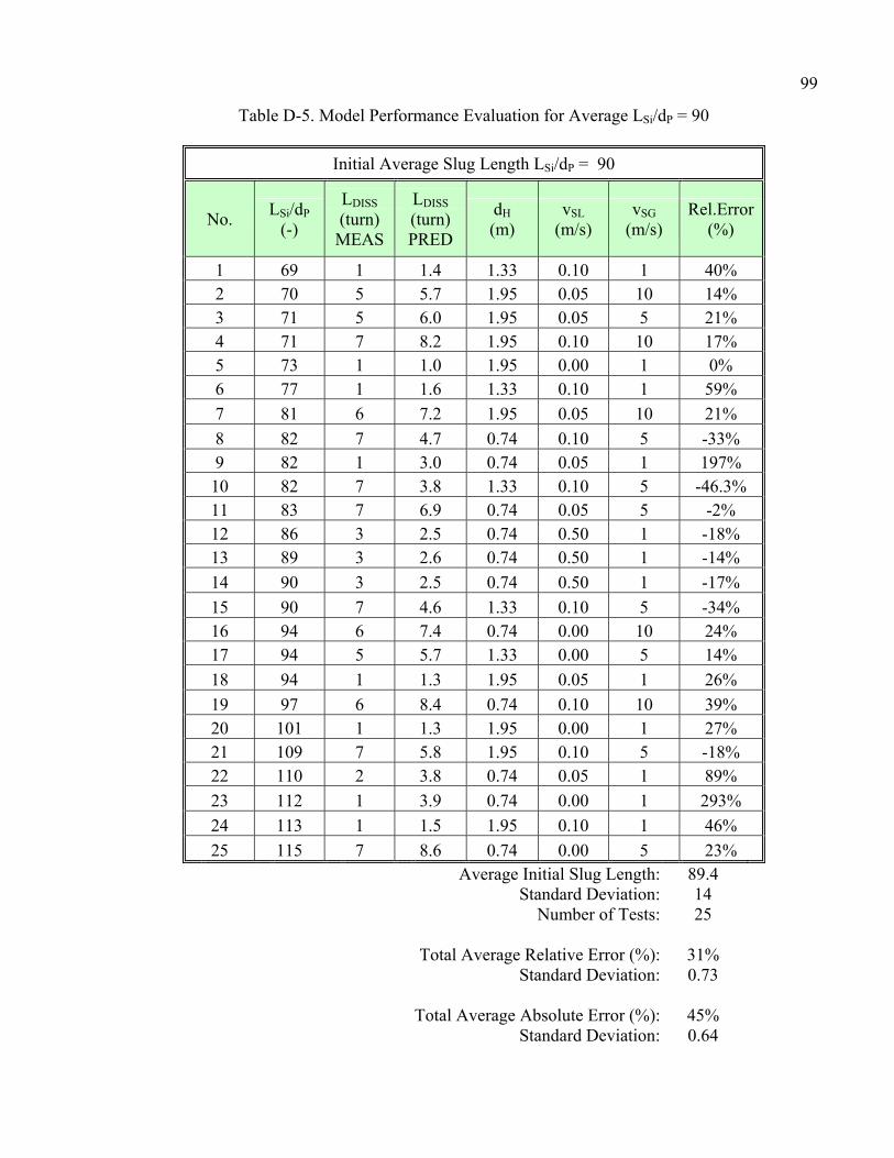
99



No. LSi/dP (-)

LDISS (turn) MEAS

LDISS (turn) PRED

dH (m)

vSL (m/s)

vSG (m/s)

Rel.Error (%)

1 69 1 1.4 1.33 0.10 1 40% 2 70 5 5.7 1.95 0.05 10 14% 3 71 5 6.0 1.95 0.05 5 21% 4 71 7 8.2 1.95 0.10 10 17% 5 73 1 1.0 1.95 0.00 1 0% 6 77 1 1.6 1.33 0.10 1 59% 7 81 6 7.2 1.95 0.05 10 21% 8 82 7 4.7 0.74 0.10 5 -33% 9 82 1 3.0 0.74 0.05 1 197% 10 82 7 3.8 1.33 0.10 5 -46.3% 11 83 7 6.9 0.74 0.05 5 -2% 12 86 3 2.5 0.74 0.50 1 -18% 13 89 3 2.6 0.74 0.50 1 -14% 14 90 3 2.5 0.74 0.50 1 -17% 15 90 7 4.6 1.33 0.10 5 -34% 16 94 6 7.4 0.74 0.00 10 24% 17 94 5 5.7 1.33 0.00 5 14% 18 94 1 1.3 1.95 0.05 1 26% 19 97 6 8.4 0.74 0.10 10 39% 20 101 1 1.3 1.95 0.00 1 27% 21 109 7 5.8 1.95 0.10 5 -18% 22 110 2 3.8 0.74 0.05 1 89% 23 112 1 3.9 0.74 0.00 1 293% 24 113 1 1.5 1.95 0.10 1 46% 25 115 7 8.6 0.74 0.00 5 23%

Average Initial Slug Length: 89.4 Standard Deviation: 14 Number of Tests: 25

Total Average Relative Error (%): 31% Standard Deviation: 0.73 Total Average Absolute Error (%): 45% Standard Deviation: 0.64

100



No. LSi/dP (-)

LDISS (turn) MEAS

LDISS (turn) PRED

dH (m)

vSL (m/s)

vSG (m/s)

Rel.Error (%)

1 117 3 2.3 1.33 0.10 1 -24% 2 119 3 2.3 1.33 0.05 1 -23% 3 121 7 7.7 1.33 0.05 5 10% 4 127 4 3.4 0.74 0.50 1 -15% 5 129 7 8.6 0.74 0.10 10 24% 6 129 4 3.5 0.74 0.50 1 -13% 7 132 7 5.1 0.74 0.50 10 -27% 8 137 7 6.5 0.74 0.10 5 -8% 9 138 7 6.2 0.74 0.50 10 -12% 10 144 7 8.9 0.74 0.05 5 28% 11 150 7 8.9 0.74 0.05 5 28% 12 161 7 6.9 1.33 0.00 10 -2% 13 177 7 8.6 1.95 0.00 10 23% 14 184 7 5.1 0.74 0.50 10 -27% 15 191 7 8.1 1.33 0.05 10 15% 16 191 7 9.1 1.95 0.00 5 30% 17 195 7 5.9 1.95 0.05 10 -16% 18 196 7 7.4 1.33 0.05 10 6% 19 196 7 8.4 1.95 0.05 5 20% 20 197 7 8.0 1.95 0.10 5 14% 21 198 7 5.4 1.33 0.10 10 -22% 22 198 7 8.9 1.95 0.00 10 28% 23 205 7 4.5 1.95 0.10 10 -36% 24 227 7 9.8 0.74 0.00 5 40% 25 232 7 10.7 1.33 0.00 5 53% 26 243 7 10.1 1.33 0.05 5 44% 27 262 7 11.1 0.74 0.05 5 58% 28 264 7 11.9 0.74 0.05 5 70% 29 270 7 8.1 0.74 0.05 10 16% 30 273 7 12.7 0.74 0.00 10 82% 31 277 7 13.8 0.74 0.00 10 98% 32 285 7 9.6 0.74 0.10 5 38% 33 311 7 10.2 0.74 0.05 10 46% 34 319 7 14.1 0.74 0.10 10 102% 35 333 7 3.4 0.74 0.50 5 -51% 36 423 7 5.7 0.74 0.50 10 -19%

101

Average Initial Slug Length; 207 Standard Deviation: 72 Number of Tests: 36 Total Average Relative Error (%): 16% Standard Deviation: 0.38 Total Average Absolute Error (%): 32% Standard Deviation: 0.24

T H E U N I V E R S I T Y O F T U L S A THE GRADUATE...

Documents

Transcript of T H E U N I V E R S I T Y O F T U L S A THE GRADUATE...