T H E U N I V E R S I T Y O F T U L S A

THE GRADUATE SCHOOL

MODELING AND CONTROL SYSTEMS DEVELOPMENT FOR

INTEGRATED THREE-PHASE COMPACT SEPARATORS

by

Carlos Avila

A thesis submitted in partial fulfillment of

the requirements for the degree of Master of Science

in the Discipline of Petroleum Engineering

The Graduate School

The University of Tulsa

2003

MODELING AND CONTROL SYSTEMS DEVELOPMENT FOR

INTEGRATED THREE-PHASE COMPACT SEPARATORS

THE UNIVERSITY OF TULSA

THE GRADUATE SCHOOL

by

Carlos Avila

A THESIS

APPROVED FOR THE DISCIPLINE OF

PETROLEUM ENGINEERING

By Thesis Committee

c ~ Ph.D.!1 ' Co-Chairman

~.,.;. Q~~:f?i~~ ~ - .~,Ovadia Shoham, Ph.D. Co-Chairman

foou~~D.~ ' Co-Chairman

rlJJ-:D. -: ~ II"" L~~in~. Ph.D. .~ 'h D . Co-Chairman, .. I

'Co,,' ffffe~~:D: - ,Member

11

iii

ABSTRACT

Avila, Carlos (Master of Science in Petroleum Engineering)

Modeling And Control Systems Development For Integrated Three-Phase Compact

Separators (152 pp. - Chapter VI)

Directed by Dr. Ram S. Mohan, Dr. Ovadia Shoham, Dr. Shoubo Wang and Dr. Luis

Gomez

(152 words)

An integrated compact separation system consisting of the Gas-Liquid Cylindrical

Cyclone (GLCC©) and the Liquid-Liquid Cylindrical Cyclone (LLCC©) in series, using a

gas control valve for controlling GLCC liquid level and liquid control valve for

controlling LLCC underflow watercut, was studied experimentally and theoretically to

investigate its performance as a three-phase oil-water-gas separator.

Experimental data acquired for the GLCC©/LLCC© system revealed higher

separation efficiencies when a low amount of gas is carried-under from the GLCC. The

GLCC©/LLCC© system simulator, developed by combining the linear models for GLCC

and LLCC control, was successfully tested for different perturbations, such as changes of

set points and flow rates, and different applications such as start-up and shut-down

operations.

Based on both the experimental and developed simulator results, the

GLCC©/LLCC© system is found to be suitable for three-phase bulk separation. Also, the

LLCC performance can be enhanced by controlling the amount of gas carry-under from

the GLCC.

iv

ACKNOWLEDGMENTS

I want to give special thanks to my advisors Dr. Ovadia Shoham, Dr. Ram S.

Mohan, Dr. Luis Gomez and Dr. Shoubo Wang, for their support and guidance

throughout my research. Their advice and support played an important role in the success

of this thesis and research.

I wish to thank the Tulsa University Separation Technology Projects (TUSTP),

and the U.S. Department of Energy (DOE), through the research grant (DE-FG26-

97BC15024), for providing financial support in conducting this research.

I also want to thank the following for their support and guidance during my

study and research:

• Ms. Judy Teal for her assistance.

• TUSTP members and graduate students for their valuable assistance,

friendship and comments during this project. Especially, Mr. Rajkumar

Mathiravedu and Mr. Vasudevan Sampath for their support.

• I also wish to thank Mr. Don Harris and Mr. Mike Teal for their expert

technical assistance in building the data acquisition systems and control

systems.

This work could not have been done without the help of the most important

persons in my life. They are my parents and my sister Ana. I also want to extend my

gratitude for her help and support of Oris and my friends, who are always in my thoughts

wherever they are.

v

TABLE OF CONTENTS

TITLE PAGE i

APPROVAL PAGE ii

ABSTRACT iii

ACKNOWLEDGMENTS iv

TABLE OF CONTENTS v

LIST OF FIGURES viii

LIST OF TABLES xiii

1. INTRODUCTION 1

2. LITERATURE REVIEW 7

2.1 GLCC Studies 7

2.2 LLCC Studies 9

2.3 Control System Studies 10

2.4 Watercut Measurement 12

3. MATHEMATICAL MODELING 14

3.1 GLCC System 14

3.1.1 GLCC Model 17

3.1.2 Liquid Level Control by Gas Control Valve 25

3.1.3 GLCC Gas Carry-Under 31

3.1.4 GLCC Liquid Carry-Over 32

3.2 LLCC System 33

3.2.1 Linear Model for LLCC Control 37

vi

3.2.2 LLCC Model With Gas 42

3.3 GLCC / LLCC System 47

3.3.1 GLCC / LLCC Separation System 48

3.3.2 Droplet Size Behavior Through Control Valves 50

3.3.3 Pressure Losses Between GLCC and LLCC 52

3.3.4 GLCC / LLCC Control System 53

3.4 Additional GLCC and LLCC Simulations 78

3.4.1 GLCC Start-Up 79

3.4.2 LLCC Start-Up 83

3.4.3 Two-Stage LLCC 84

4. EXPERIMENTAL PROGRAM 90

4.1 Experimental Setup 90

4.1.1 Storage and Metering Section 90

4.1.2 Test Section 92

4.1.3 Gas-Oil-Water Separation Section 95

4.1.4 Data Acquisition System 96

4.1.5 Working Fluids 96

4.2 Watercut Measurement Performance in the Presence of Gas 98

4.2.1 Coriolis Mass Flow Meter (Micromotion) 99

4.2.2 Microwave Watercut Meter (Starcut) 100

4.2.3 Watercut Measurement Using Micromotion Compensated

for Gas Void Fraction 103

4.3 Inversion Point Determination 106

vii

4.4 Transient Data 107

4.4.1 GLCC Liquid Level Setpoint as a Perturbation 108

4.4.2 LLCC Underflow Watercut Setpoint as a Perturbation 111

4.4.3 Inlet Flowrates and Watercut as a Perturbation for the

GLCC/LLCC System 113

4.4.4 Improvements in GLCC / LLCC System 117

5. RESULTS AND DISCUSSION 127

5.1 Mathematical Model Discussion 127

5.2 Experimental Program Discussion 128

5.2.1 Uncertainty Analysis for Watercut Meters 128

5.2.2 Uncertainty Analysis at the Inversion Point 132

5.2.3 Uncertainty Analysis for GLCC Liquid Level

Determination 133

5.2.4 Transient Data Discussion 135

6. CONCLUSIONS AND RECOMMENDATIONS 136

NOMENCLATURE 140

REFERENCES AND BIBLIOGRAPHY 145

APPENDIX 152

viii

LIST OF FIGURES

Figure 1.1 Schematic of the Gas Liquid Cylindrical Cyclone (GLCC©) 2

Figure 1.2 Schematic of the Liquid-Liquid Cylindrical Cyclone (LLCC©) 4

Figure 1.3 Schematic of Two-Stage GLCC© and LLCC© Compact Separation System 5

Figure 3.1 Schematic of GLCC with Metering Loop and Control Systems 15

Figure 3.2 GLCC System Dynamic Modeling Overview 17

Figure 3.3 Block Diagram of Liquid Level Control System by GCV 26

Figure 3.4 Linear Model of Liquid Level Control by GCV 26

Figure 3.5 Schematic of LLCC Control System 33

Figure 3.6 Schematic of LLCC Control Loop 35

Figure 3.7 Structure of Feedback Control Configuration 36

Figure 3.8 Linear Model of LLCC Control Loop 38

Figure 3.9 GVF Effect on the LLCC Split Ratio for 60% Inlet Watercut 45

Figure 3.10 Prediction of LLCC Split Ratio as a Function of the GVF 46

Figure 3.11 Root Locus Plot for LLCC with Gas 47

Figure 3.12 Initial GLCC / LLCC System Approach 48

Figure 3.13 Current GLCC / LLCC System Configuration 49

Figure 3.14 LCV Position and Pressure Drop in Control Valve 51

Figure 3.15 Maximum Droplet Size Downstream of a Control Valve 52

Figure 3.16 Common Vector for Each Pipeline 54

Figure 3.17 GLCC / LLCC System Simulator 56

Figure 3.18 Input Vector Module 57

ix

Figure 3.19 Properties Vector Module 58

Figure 3.20 GLCC Model Subsystem 59

Figure 3.21 GLCC Level Control Subsystem 60

Figure 3.22 GLCC Liquid Carry-over Subsystem 61

Figure 3.23 GLCC Gas Carry-under Subsystem 62

Figure 3.24 GLCC/LLCC Pressure Losses Subsystem 63

Figure 3.25 LLCC Model Subsystem 64

Figure 3.26 LLCC Watercut Control Subsystem 65

Figure 3.27 LLCC Split Ratio to watercut Subsystem 66

Figure 3.28 Gas in LLCC Underflow Subsystem 67

Figure 3.29 Continuous-Phase Detector 67

Figure 3.30 GLCC/LLCC Simulator Results Displays 68

Figure 3.31 GLCC Liquid Level Setpoints Induced 69

Figure 3.32 Actual GLCC Liquid Level for Setpoints Induced 70

Figure 3.33 GLCC Underflow GVF for Liquid Level Setpoints Induced 70

Figure 3.34 LLCC Split Ratio for Liquid Level Setpoints Induced 71

Figure 3.35 Watercut in LLCC (underflow) 72

Figure 3.36 LLCC Underflow Watercut Setpoints Induced 73

Figure 3.37 Actual LLCC Underflow Watercuts for Setpoints Induced 73

Figure 3.38 LLCC Split Ratio for Watercut Setpoints Induced 74

Figure 3.39 GLCC Gas and Oil Flowrates Induced 75

Figure 3.40 GLCC Water Flowrates Induced 75

Figure 3.41 GLCC Liquid Level for Different Water Flowrates Induced 76

x

Figure 3.42 GLCC Underflow GVF for Different Water Flowrates Induced 77

Figure 3.43 LLCC Split Ratio for Different Water Flowrates Induced 77

Figure 3.44 LLCC Underflow Watercut for Different Water Flowrates Induced 78

Figure 3.45 GLCC Start-up Simulator 79

Figure 3.46 GLCC Liquid Level Setpoint Inputs 80

Figure 3.47 Actual GLCC Liquid Level for Different Setpoint Inputs 80

Figure 3.48 GLCC Underflow GVF for Different Setpoint Inputs 81

Figure 3.49 LLCC Start-up Simulator 82

Figure 3.50 LLCC Underflow Watercut Setpoint Inputs 83

Figure 3.51 Actual LLCC Underflow Watercut for Different Setpoint Inputs 84

Figure 3.52 Two-Stage LLCC Simulator 85

Figure 3.53 Input Flowrates into Two-Stage LLCC System 86

Figure 3.54 First Stage LLCC Underflow Watercut 87

Figure 3.55 Second Stage LLCC Underflow Watercut 87

Figure 3.56 First and Second Stage LLCC Overflow Watercut and Second Stage

LLCC Inlet Watercut 88

Figure 3.57 First and Second Stage LLCC Split Ratios 89

Figure 4.1 Experimental Facility 91

Figure 4.2 Storage And Metering Section 92

Figure 4.3 GLCC Test Section 93

Figure 4.4 LLCC Test Section 94

Figure 4.5 Photo of LLCC Test Section in Place 95

Figure 4.6 Coriolis Mass Flow Meter (Micromotion) in Flow Loop 100

xi

Figure 4.7 Microwave Watercut Meter (Starcut) in Flow Loop 101

Figure 4.8 Starcut Watercut Measurement Validation (50% to 100%) 102

Figure 4.9 Starcut Watercut Measurement Validation (90% to 100%) 102

Figure 4.10 Watercut Measurement Performance Comparison in the Presence of Gas 104

Figure 4.11 Compensated Watercut Measurement Performance in Presence of Gas 105

Figure 4.12 Micromotion Drive Gain for Different Gas Void Fractions 106

Figure 4.13 Inversion Point for Oil-Water mixture based on Starcut. 107

Figure 4.14 GLCC Liquid Level Setpoints Induced 108

Figure 4.15 GLCC Liquid Level Response for Setpoints Induced 109

Figure 4.16 LLCC Underflow Watercut with GLCC Liquid Level Control 110

Figure 4.17 LLCC Split Ratio with GLCC Liquid Level Control 110

Figure 4.18 LLCC Underflow Watercut Setpoints Induced 111

Figure 4.19. LLCC Underflow Watercut for Different Setpoints 112

Figure 4.20 LLCC Split Ratio for Different Watercut Setpoints Induced 112

Figure 4.21 Inlet Air Mass Flowrate 113

Figure 4.22 Inlet Oil Mass Flowrate 114

Figure 4.23 Inlet Water Mass Flow 114

Figure 4.24 GLCC Liquid Level for Different Inlet Water Flowrate Perturbations 115

Figure 4.25 LLCC Underflow Watercut for Flowrate Perturbations (Case1) 116

Figure 4.26 LLCC Split Ratio for Different Inlet Water Flowrate Perturbations 117

Figure 4.27 GLCC Liquid Level for Different Setpoints 118

Figure 4.28 GLCC Liquid Level Measurement Comparison 119

Figure 4.29 LLCC Underflow Watercut (97%-98%-97% Setpoint) 120

xii

Figure 4.30 LLCC Underflow Watercut (97%-99%-97% Setpoint) 121

Figure 4.31 LLCC Underflow Watercut (97%-92%-97% Setpoint) 121

Figure 4.32 LLCC Split Ratio Obtained using Micromotion to Measure Watercut 123

Figure 4.33 LLCC Split Ratio Obtained using GVF Compensated Micromotion 123

Figure 4.34 GLCC Liquid Level for Different Setpoints 124

Figure 4.35 LLCC Split Ratio for Different GLCC Liquid Level Setpoints 125

Figure 4.36 LLCC Split Ratio for Different GLCC Liquid Level Setpoints (Watercut

Measured using Micromotion GVF Compensated) 126

Figure 5.1 Starcut Watercut Meter Validation using Single-Phase Measurements with

Micromotion (0% Gas, 50%-100% Watercut Range) 130

Figure 5.2 Starcut Watercut Meter Validation using Single-Phase Measurements with

Micromotion (0% Gas, 90%-100% Watercut Range) 130

Figure 5.3 Watercut Measurement Performance Comparison in the Presence of Gas 131

Figure 5.4 Compensated Watercut Measurement Performance in Presence of Gas 132

Figure 5.5 Inversion Point for Oil-Water Mixture based on Starcut 133

Figure 5.6 GLCC Liquid Level Comparison With and Without Mixture Density

Correction 134

xiii

LIST OF TABLES

Table 3.1 Values of Empirical Factor, Fgl 44

Table 3.2 PID Settings for GLCC and LLCC Controllers During Simulations 69

Table 4.1 Properties of Water Phase 97

Table 4.2 Properties of Oil Phase 97

Table 4.3 PID Settings for GLCC and LLCC Controllers during Experiments 108

Table 4.4 Offset in Liquid Level Signal With and Without Mixture Density

Correction 119

Table 5.1 Uncertainty Analysis for Watercut Meters 129

Table 5.2 Uncertainty Analysis for GLCC Liquid Level Determination 134

1

1. INTRODUCTION

A common phenomenon in the petroleum industry is the production of water

along with hydrocarbons. The amount of produced water usually increases as the field

becomes more mature, and also due to utilization of secondary recovery methods, such as

water flooding. The volume of produced water that must be processed in the downstream

separation facilities often exceeds that of the produced hydrocarbons. This poses a

problem for the industry, as it results in an increase in the size and cost of the separation

facilities.

In the past, oil-water-gas separation technology in the petroleum industry has

relied mainly on conventional vessel-type gravity separators, which are bulky, heavy and

expensive. Recently, the industry has shown keen interest in developing and applying

compact separators that have low weight, possess low cost and are highly efficient. This

has been promoted by the challenges to reduce production costs of offshore and marginal

fields. Following is a brief review of available compact separators.

Gas-Liquid Separation: One economically attractive alternative to conventional

vessel-type gravity separators is the Gas-Liquid Cylindrical Cyclone (GLCC©)1, as

shown in Figure 1.1. The GLCC is a simple, compact, low weight and low-cost

separator. It is a vertical pipe section, mounted with a downward inclined, tangential inlet

located approximately at the middle. Neither moving parts nor internal devices are used,

reducing the need for maintenance. Separation in this equipment is achieved by

1 GLCC© - Gas-Liquid Cylindrical Cyclone - Copyright, The University of Tulsa, 1994

2

centrifugal and gravity forces. The inclined inlet promotes pre-separation of the gas and

liquid phases due to stratification, and the tangential inlet creates a swirling motion in the

vertical pipe. As a result of the centrifugal forces, the heavier liquid phase is forced

toward the pipe wall. The liquid then flows downward and exits from the bottom through

the liquid outlet. The gas phase, being lighter, moves to the center of the pipe and exits

from the top through the gas outlet. Control valves on both gas and liquid outlets

maintain the liquid level around the set point inside the GLCC.

Gas/LiquidGas/Liquid

GasGas

LiquidLiquid

Gas/LiquidGas/Liquid

GasGas

LiquidLiquid

Figure 1.1 Schematic of the Gas Liquid Cylindrical Cyclone (GLCC©)

Mechanistic models for design and performance prediction of GLCC have already

been developed (Gomez, 1998, Gomez, L.E., 2001) and are in use by the industry. In

these models, the oil-water mixture is treated as a single liquid-phase flow. Also,

strategies for the GLCC liquid level and pressure control have been developed (Wang,

3

2000, Wang et al., 2000). Following the theoretical development of the GLCC control

strategies, field implementations have demonstrated the concept validity. The GLCC has

recently gained popularity in the industry, with more than 500 units installed in the field

around the world.

Liquid-Liquid Separation: The Liquid-Liquid Hydrocyclone (LLHC) is utilized

by the industry to clean produced oily water for disposal, reducing oil concentrations to

levels below 40 ppm. This equipment is suitable for cleaning water with low oil content.

Attempts have been made in the past to utilize cylindrical hydrocyclones for oil-water

separation. The use of cylindrical hydrocyclones for oil-water separation has been

hindered due to the fact that at high velocities they perform as mixers rather than

separators. However, by operating at moderate velocities, the cylindrical hydrocyclone

can be used to perform at least partial oil-water separation (free-water knockout).

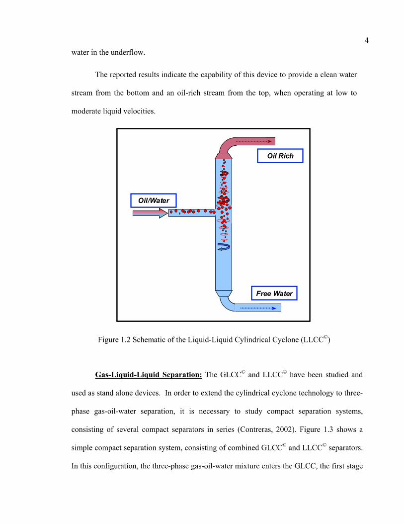
Recently, studies have been conducted (Mathiravedu, 2001) on the performance

of Liquid-Liquid Cylindrical Cyclone (LLCC©)2 as a free-water knockout. The LLCC©

has a similar configuration as that of the GLCC, namely, a vertical pipe section, but with

a horizontal tangential inlet, as shown in Figure 1.2. The horizontal inlet promotes oil-

water stratification. The liquid phase mixture enters the vertical section through a

reducing area nozzle, increasing its velocity. The swirling motion in the LLCC produces

a centrifugal separation, whereby the oil phase moves to the center, and an oil-rich stream

exits through the top (overflow). The water moves to the pipe wall, flows downward and

exits through the bottom (underflow). Mathiravedu (2001) has also demonstrated the use

of a unique quality control strategy in order to ensure the condition of maximum clean

2 LLCC© - Liquid-Liquid Cylindrical Cyclone - Copyright, The University of Tulsa, 1998

4

water in the underflow.

The reported results indicate the capability of this device to provide a clean water

stream from the bottom and an oil-rich stream from the top, when operating at low to

moderate liquid velocities.

Oil/WaterOil/Water

Free WaterFree Water

Oil RichOil Rich

Oil/WaterOil/Water

Free WaterFree Water

Oil RichOil Rich

Figure 1.2 Schematic of the Liquid-Liquid Cylindrical Cyclone (LLCC©)

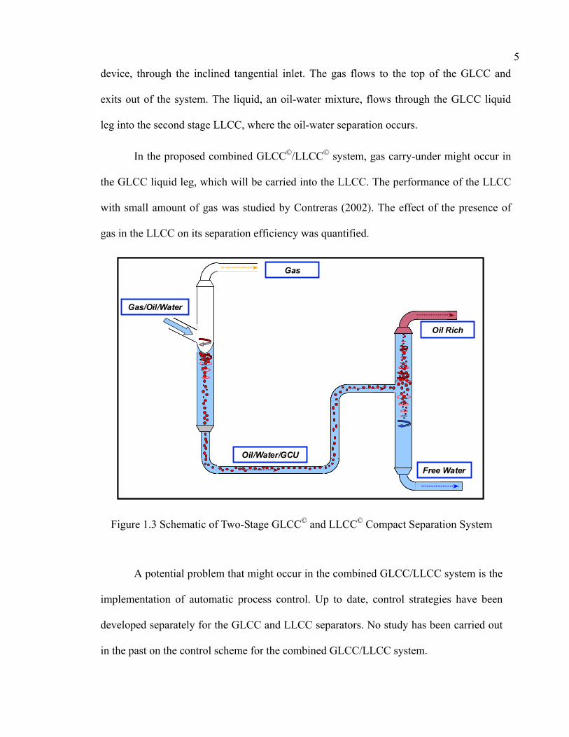
Gas-Liquid-Liquid Separation: The GLCC© and LLCC© have been studied and

used as stand alone devices. In order to extend the cylindrical cyclone technology to three-

phase gas-oil-water separation, it is necessary to study compact separation systems,

consisting of several compact separators in series (Contreras, 2002). Figure 1.3 shows a

simple compact separation system, consisting of combined GLCC© and LLCC© separators.

In this configuration, the three-phase gas-oil-water mixture enters the GLCC, the first stage

5

device, through the inclined tangential inlet. The gas flows to the top of the GLCC and

exits out of the system. The liquid, an oil-water mixture, flows through the GLCC liquid

leg into the second stage LLCC, where the oil-water separation occurs.

In the proposed combined GLCC©/LLCC© system, gas carry-under might occur in

the GLCC liquid leg, which will be carried into the LLCC. The performance of the LLCC

with small amount of gas was studied by Contreras (2002). The effect of the presence of

gas in the LLCC on its separation efficiency was quantified.

Gas/Oil/WaterGas/Oil/Water

GasGas

Oil/Water/GCUOil/Water/GCU

Free WaterFree Water

Oil RichOil Rich

Gas/Oil/WaterGas/Oil/Water

GasGas

Oil/Water/GCUOil/Water/GCU

Free WaterFree Water

Oil RichOil Rich

Figure 1.3 Schematic of Two-Stage GLCC© and LLCC© Compact Separation System

A potential problem that might occur in the combined GLCC/LLCC system is the

implementation of automatic process control. Up to date, control strategies have been

developed separately for the GLCC and LLCC separators. No study has been carried out

in the past on the control scheme for the combined GLCC/LLCC system.

6

Objective and Thesis Structure: The objective of the present study is to

combine previous control strategies, developed separately for the GLCC and the LLCC,

and develop a coupled strategy for the GLCC/LLCC system. Furthermore, the design and

installation of an integrated control system, capable of ensuring three-phase separation

for the GLCC©/LLCC© system, is developed. Finally, extension of the present analysis of

the GLCC©/LLCC© combined system for other separation systems or configurations is

presented.

The next chapter presents a review of the literature relevant to this study. The

GLCC/LLCC mathematical model is presented in Chapter 3. Chapter 4 presents the

experimental program, including the GLCC/LLCC test facility, testing procedure and

experimental results. A discussion of the developed coupled model predictions and the

experimental results is presented in Chapter 5. Conclusions and recommendations can be

found in Chapter 6.

7

2. LITERATURE REVIEW

The use of the Gas-Liquid Cylindrical Cyclone (GLCC) and the Liquid-Liquid-

Cylindrical Cyclone (LLCC) as a three-phase separation system is a first step in the

development of integrated separation systems at The Tulsa University Separation

Technology Projects (TUSTP). Pertinent literature on the GLCC and LLCC, along with

related topics is given below.

2.1 GLCC Studies

Previous experimental attempts using cylindrical hydrocyclones for gas-liquid

separation found in the literature include Davies and Watson (1979) and Davies (1984),

who studied compact separators for offshore production, where small size and low weight

of the equipment are important. They showed that there are several advantages of using a

cyclone separator instead of conventional separator, such as compactness and low cost,

while improving the separation performance.

Nebrensky et al. (1980), developed a cyclone for gas-oil separation that included a

tangential rectangular inlet with a special arrangement to change the inlet area. Zhikarev

et al. (1985) developed a cyclone separator with a rectangular, tangential inlet located

near the bottom.

Based on experimental results, Fekete (1986) suggested the use of a vortex tube

separator due to its low weight and small size. Another study by Oranje (1990) also

showed that cyclone type separators are suitable for applications on offshore platforms

8

due to their small size and weight.

Cowie (1991) tested vertical caisson slug catchers, comparing radial and

tangential inlets. The tangential inlet configuration provided the best performance.

Bandyopadhyay et al. (1994) studied the separation of helium bubbles from water using

cyclone separators. Weingarten et al. (1995), developed and tested the auger separator,

which is a cylindrical cyclone with internal spiral vanes.

Based on experimental and theoretical studies performed at The University of

Tulsa, a mechanistic model for the GLCC was developed by Arpandi et al. (1995). This

model is able to predict the general hydrodynamic flow behavior in a GLCC, including

simple velocity profiles, gas-liquid interface shape, equilibrium liquid level, total

pressure drop, and operational envelop for liquid carry-over. Marti et al. (1996),

attempted to develop a mechanistic model to predict gas carry-under in GLCC separators.

This model predicts the separation efficiency based on bubble trajectory analysis. Gomez

(1998) developed a state-of-the-art computer code integrating improved models for the

different sections of the GLCC. The models developed at The University of Tulsa have

allowed the application of GLCC to real field cases, as detailed by Kouba and Shoham

(1996) and Gomez (1998).

Movafaghian et al. (2000) reported the effects of fluid properties, inlet geometry

and pressure on the behavior of the GLCC. Recently, Gomez, L.E. (2001) developed a

model to predict the gas carry-under in this separator.

9

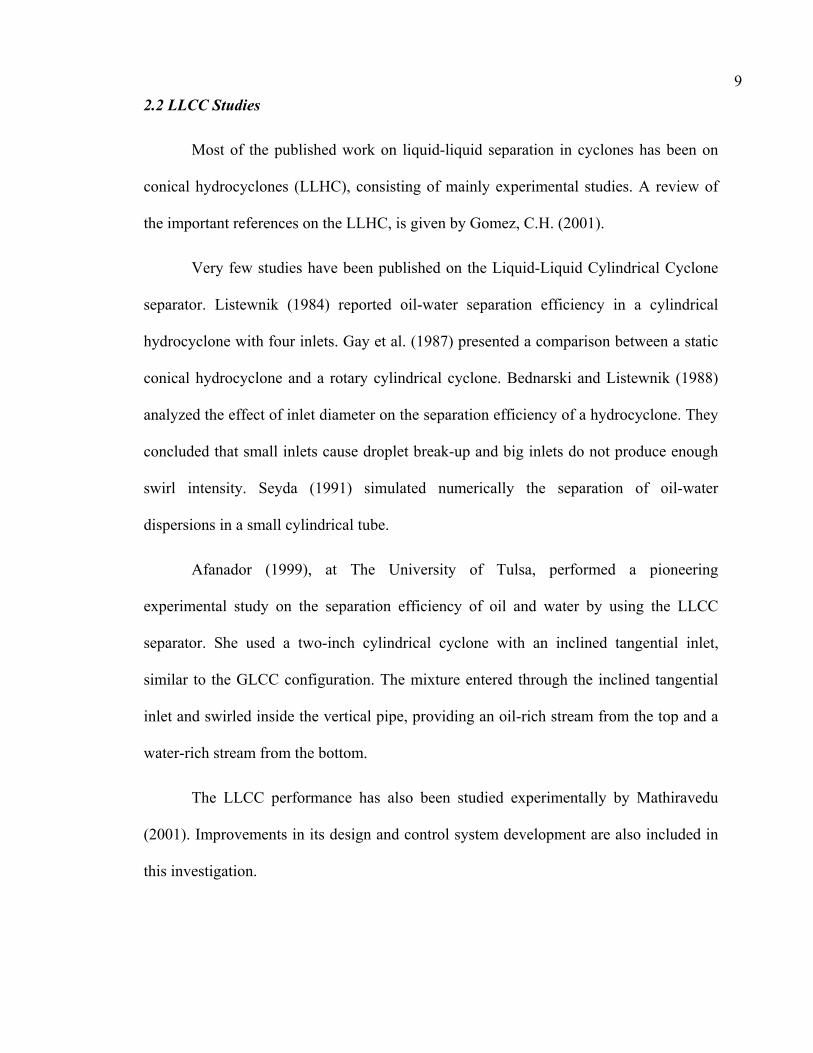
2.2 LLCC Studies

Most of the published work on liquid-liquid separation in cyclones has been on

conical hydrocyclones (LLHC), consisting of mainly experimental studies. A review of

the important references on the LLHC, is given by Gomez, C.H. (2001).

Very few studies have been published on the Liquid-Liquid Cylindrical Cyclone

separator. Listewnik (1984) reported oil-water separation efficiency in a cylindrical

hydrocyclone with four inlets. Gay et al. (1987) presented a comparison between a static

conical hydrocyclone and a rotary cylindrical cyclone. Bednarski and Listewnik (1988)

analyzed the effect of inlet diameter on the separation efficiency of a hydrocyclone. They

concluded that small inlets cause droplet break-up and big inlets do not produce enough

swirl intensity. Seyda (1991) simulated numerically the separation of oil-water

dispersions in a small cylindrical tube.

Afanador (1999), at The University of Tulsa, performed a pioneering

experimental study on the separation efficiency of oil and water by using the LLCC

separator. She used a two-inch cylindrical cyclone with an inclined tangential inlet,

similar to the GLCC configuration. The mixture entered through the inclined tangential

inlet and swirled inside the vertical pipe, providing an oil-rich stream from the top and a

water-rich stream from the bottom.

The LLCC performance has also been studied experimentally by Mathiravedu

(2001). Improvements in its design and control system development are also included in

this investigation.

10

Also recently, Oropeza (2001) developed a novel mechanistic model for

prediction of the complex flow behavior and separation efficiency in the LLCC. The

model consists of several sub-models, including inlet analysis, nozzle analysis, droplet

size distribution model, and separation model based on droplet trajectories in swirling

flow field. Comparisons between the LLCC model predictions and experimental data

showed excellent agreement qualitatively and quantitatively. The developed model can

be utilized for performance analysis and design of the LLCC.

Contreras et al. (2002) studied the effect of the presence of small amount of gas in

the oil-water mixture at the inlet of the LLCC on its performance and separation

efficiency.

2.3 Control System Studies

Control system studies for compact separators have been one of the recent

developments in the oil industry. The performance of compact separators can be

enhanced considerably by incorporating suitable control systems. Development of control

systems for GLCC technology has demonstrated a tremendous impact in improving the

optimization and performance of this separator.

Kartinen and Lewis (1974) developed a discharge flow control system for a

centrifugal separator. The flow control system included a diaphragm-operated valve in

the outlet line that carries the lighter density fluid from the separator. The discharge

pressure of the separated lighter density fluid operated the valve. This pressure was

compared to the inlet mixture pressure across the control diaphragm.

11

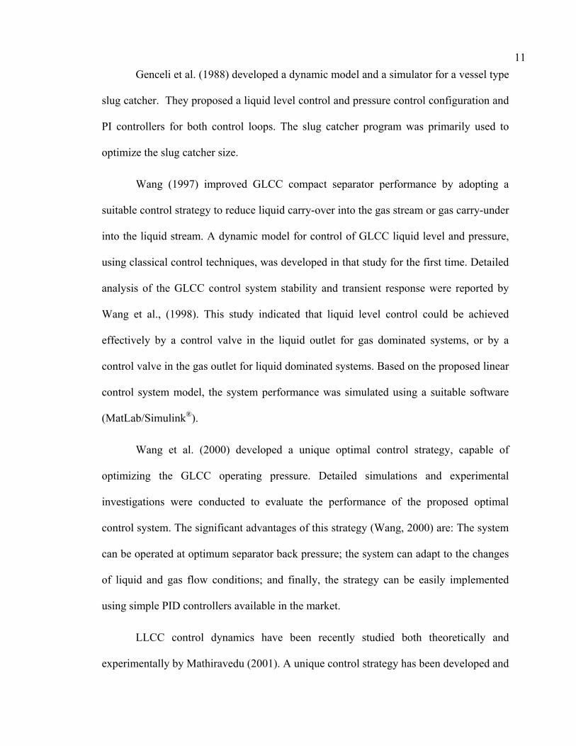
Genceli et al. (1988) developed a dynamic model and a simulator for a vessel type

slug catcher. They proposed a liquid level control and pressure control configuration and

PI controllers for both control loops. The slug catcher program was primarily used to

optimize the slug catcher size.

Wang (1997) improved GLCC compact separator performance by adopting a

suitable control strategy to reduce liquid carry-over into the gas stream or gas carry-under

into the liquid stream. A dynamic model for control of GLCC liquid level and pressure,

using classical control techniques, was developed in that study for the first time. Detailed

analysis of the GLCC control system stability and transient response were reported by

Wang et al., (1998). This study indicated that liquid level control could be achieved

effectively by a control valve in the liquid outlet for gas dominated systems, or by a

control valve in the gas outlet for liquid dominated systems. Based on the proposed linear

control system model, the system performance was simulated using a suitable software

(MatLab/Simulink®).

Wang et al. (2000) developed a unique optimal control strategy, capable of

optimizing the GLCC operating pressure. Detailed simulations and experimental

investigations were conducted to evaluate the performance of the proposed optimal

control system. The significant advantages of this strategy (Wang, 2000) are: The system

can be operated at optimum separator back pressure; the system can adapt to the changes

of liquid and gas flow conditions; and finally, the strategy can be easily implemented

using simple PID controllers available in the market.

LLCC control dynamics have been recently studied both theoretically and

experimentally by Mathiravedu (2001). A unique control strategy has been developed and

12

implemented, capable of obtaining clear water in the underflow line and maintaining

maximum underflow (optimal split ratio). A linear model has been developed, for the

first time, for LLCC separators equipped with underflow watercut control, which enables

simulation of the system dynamic behavior. Comparison of simulation and experimental

results showed that the control system simulator is capable of representing the real

physical system and can be used to verify the controller design and dynamic behavior.

2.4 Watercut Measurement

The measurement of water content in crude oil is an important and widely

encountered practice in the petroleum industry. The watercut measurement is utilized in

multiphase flow meters. Also, monitoring watercut at various points throughout a

processing facility may optimize the separation efficiency in production operations. A

review of available watercut meters is reported below.

Agar (1988) developed a watercut meter using microwave method, by measuring

the energy absorption properties of an oil-water mixture. Lew (1988) developed a method

and a device for determining the concentration of each phase in an oil-water mixture

utilizing Nuclear Magnetic Resonance (NMR) analysis. In this method, a direct and

accurate measure of the desired component, oil for example, can be achieved on a real-

time basis in the field, without the need to interrupt operations.

Durrett et al. (1989) developed a watercut monitor that uses microwave principle

to measure the watercut in a multiphase flow stream. Measurement accuracy was

maintained despite changes in temperature, salinity, crude properties and the presence of

13

gas. Gaisford et al. (1992) used Radio Frequency (RF) bridge technique to determine the

composition of oil and water in an oil-water mixture. The device is operated by using the

metal pipe of the process stream as an electromagnetic waveguide.

Cobb (1995) developed a method and an apparatus to monitor the composition of

a fluid mixture traveling through a conduit, using ultrasonic propagation. These

measurements were used to determine fluid mixture composition based on a relationship

derived from measurement of samples of the fluid mixture. Al-Mubarak (1997) proposed

a new method for calculating watercut using a Coriolis device such as Micromotion®

mass flow meter. The method provided reliable well testing results that are comparable

with a three-phase conventional test facility, when there is no gas present in the

multiphase mixture. Recently, Lievois (2000) developed a narrow band infrared watercut

meter that can detect a full watercut range of a flow stream.

As shown above, there is no previous work regarding the integration process of

separators. However, the work of Contreras (2002) is very helpful since it considers one

of the most important factors in the cascaded configuration, which is the effect of the gas

carry-under coming from the GLCC into the LLCC, on the LLCC performance. The

scope and contribution of the present study is to assemble previous models and

experimental studies performed for each separator separately, and construct a coupled

model for the GLCC/LLCC system.

14

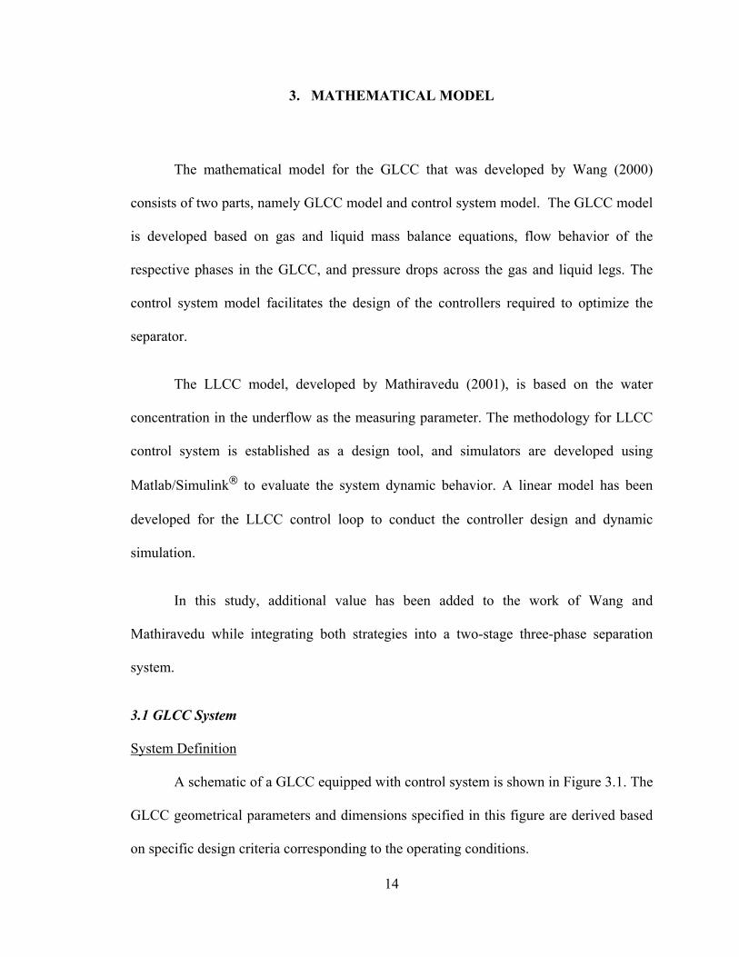
3. MATHEMATICAL MODEL

The mathematical model for the GLCC that was developed by Wang (2000)

consists of two parts, namely GLCC model and control system model. The GLCC model

is developed based on gas and liquid mass balance equations, flow behavior of the

respective phases in the GLCC, and pressure drops across the gas and liquid legs. The

control system model facilitates the design of the controllers required to optimize the

separator.

The LLCC model, developed by Mathiravedu (2001), is based on the water

concentration in the underflow as the measuring parameter. The methodology for LLCC

control system is established as a design tool, and simulators are developed using

Matlab/Simulink® to evaluate the system dynamic behavior. A linear model has been

developed for the LLCC control loop to conduct the controller design and dynamic

simulation.

In this study, additional value has been added to the work of Wang and

Mathiravedu while integrating both strategies into a two-stage three-phase separation

system.

3.1 GLCC System

System Definition

A schematic of a GLCC equipped with control system is shown in Figure 3.1. The

GLCC geometrical parameters and dimensions specified in this figure are derived based

on specific design criteria corresponding to the operating conditions.

15

DPGas / LiquidInlet

Liquid Leg

Gas Leg

Gas Meter

Liquid Meter

Recombination

Top View

DPDPGas / LiquidInlet

Liquid Leg

Gas Leg

Gas Meter

Liquid Meter

Recombination

Top View

Figure 3.1 Schematic of GLCC with Metering Loop and Control Systems

The GLCC separator has a two-phase flow inlet and single-phase gas and liquid

outlets. A level sensor, such as a differential pressure transducer, is used to determine the

dynamic liquid level in the GLCC. The actuating signal from the level sensor is sent to

the liquid level controller, which in turn operates the liquid control valve (LCV) opening

the liquid outlet, correspondingly. However, for very large liquid flow variations, the

liquid level may rise even when the liquid leg valve is completely open. During that

circumstance, it is possible to avoid liquid carry-over through building up backpressure in

the GLCC by closing the gas control valve (GCV). Alternatively, the gas control valve

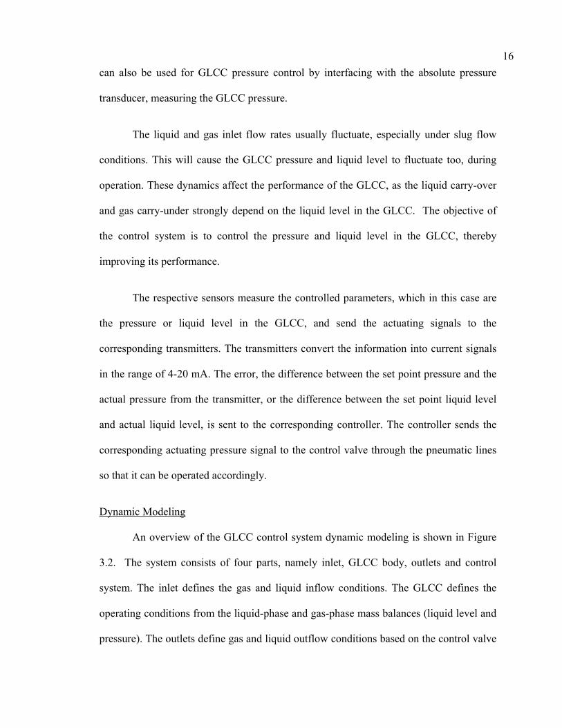
16can also be used for GLCC pressure control by interfacing with the absolute pressure

transducer, measuring the GLCC pressure.

The liquid and gas inlet flow rates usually fluctuate, especially under slug flow

conditions. This will cause the GLCC pressure and liquid level to fluctuate too, during

operation. These dynamics affect the performance of the GLCC, as the liquid carry-over

and gas carry-under strongly depend on the liquid level in the GLCC. The objective of

the control system is to control the pressure and liquid level in the GLCC, thereby

improving its performance.

The respective sensors measure the controlled parameters, which in this case are

the pressure or liquid level in the GLCC, and send the actuating signals to the

corresponding transmitters. The transmitters convert the information into current signals

in the range of 4-20 mA. The error, the difference between the set point pressure and the

actual pressure from the transmitter, or the difference between the set point liquid level

and actual liquid level, is sent to the corresponding controller. The controller sends the

corresponding actuating pressure signal to the control valve through the pneumatic lines

so that it can be operated accordingly.

Dynamic Modeling

An overview of the GLCC control system dynamic modeling is shown in Figure

3.2. The system consists of four parts, namely inlet, GLCC body, outlets and control

system. The inlet defines the gas and liquid inflow conditions. The GLCC defines the

operating conditions from the liquid-phase and gas-phase mass balances (liquid level and

pressure). The outlets define gas and liquid outflow conditions based on the control valve

17characteristics. The control system provides the interface between the GLCC and the

outlets based on the control system characteristics (controller, sensor, actuator etc.). The

dynamic model is developed for the GLCC and the control system in the following

sections.

Inlet GLCC Outlet

Control System

Flow conditions

Operational conditions

Control Valvecharacteristics

Controllercharacteristics

Inlet GLCC Outlet

Control System

Flow conditions

Operational conditions

Control Valvecharacteristics

Controllercharacteristics

Figure 3.2 GLCC System Dynamic Modeling Overview

3.1.1 GLCC Model

Pressure balances across the liquid leg and gas leg provide two equations related to the

GLCC pressure and the liquid level. The mass balances of the liquid-phase and the gas-

phase provide two additional equations. These equations are given next.

Liquid Leg Pressure Drop. The pressure drop across the liquid leg is given by

LCVc

LLoutLLLout ∆P

ggHρQρC

PP +−

=−2

(3.1)

where LC is the overall flow coefficient of the liquid leg that is given by,

18

+= ∑ ∑

= =

n

i

m

j Lj

jL

Li

iLiLL dd

LfC

1 12425

88π

κ

π (3.2)

LCVP∆ is the pressure drop across the liquid control valve, which can be solved from the

liquid control valve flow rate equation (Fisher, 1998), as follows

( )L

LCVvLout

PCQ

γ∆

= 002228.0 (3.3)

Solving LCVP∆ from equation (3.3) gives

( ) 22

2

002228.0 v

LLoutLCV C

QP

γ=∆ (3.4)

Substituting equation (3.4) into equation (3.1) yields an expression for the total pressure

drop across the liquid leg of the GLCC, namely,

+−

=−c

LLoutLLLout g

gHρQρCPP

2

( ) 22

2

002228.0 v

LLout

CQ γ

(3.5)

Taking the derivative of equation (3.5) with respect to time, and assuming the

liquid discharge pressure, LoutP , to be constant, gives an expression for the rate of change

of the GLCC pressure caused by the change of the liquid control valve position, namely,

19

( )

( ) ( )

( )222

2222

002228.0

002228.02002228.02

2

v

vLLoutvv

LoutLLout

c

LLout

LoutLL

C

dtdC

QCCdt

dQQ

gdt

dHgρdt

dQQρC

dtdP

γγ −

+

−=

(3.6)

Gas Leg Pressure Drop. The pressure drop across the gas leg is given by

GCVc

GGoutGGGout ∆P

ggHρQρC

PP +−

=−2

(3.7)

where GC is the overall flow coefficient of the gas leg that is given by,

+= ∑ ∑

= =

n

i

m

j Gj

jG

Gi

iGiGG dd

LfC

1 12425

88π

κ

π (3.8)

GCVP∆ is the pressure across the gas leg of the GLCC, which can be solved from the gas

control valve flow rate equation (Fisher, 1998),

( )Deg

GCVg

GGout P

PC

CPTQ

∆

=

1

3417sin5203600

7.14γ

(3.9)

Solving GCVP∆ from equation (3.9) gives,

20

( )( )

( )22

1 5207.14

3600sin

3417

=∆

TPCQ

arcPCP G

g

GoutGCV

γ (3.10)

Substituting equation (3.10) in equation (3.7) gives the total pressure drop across the gas

leg, namely,

+−

=−c

GGoutGGGout g

gHρQρCPP

2 ( )( )

( )22

1 5207.14

3600sin

3417

TPCQ

arcPC G

g

Gout γ (3.11)

Taking the derivative of equation (3.11) with respect to time, assuming constant

liquid discharge pressure LoutP and operating temperature T , gives an expression for the

rate of change of the GLCC pressure caused by the change of gas control valve position,

namely,

( )( )

( )

( )( )

( )

( )( )

( )

+−

−

+

+

−+

−=

22

2

21

221

2

5207.14

3600

5207.14

36001

13417

5207.14

3600sin

3417

2

g

gg

GoutgGout

G

g

G

g

Gout

G

g

Gout

GoutGoutG

c

GG

c

GoutG

CPdtdPC

dtdC

PQPCdt

dQ

TC

TPCQ

PC

dtdP

TPCQ

arcC

dtdHg

dtdQ

QCgρ

dtdρ

ggHQC

dtdP

γ

γ

γ

(3.12)

21The rate of change of gas density can be found from the equation of state, given by,

ZRTPM G

G =ρ (3.13)

Taking the derivative of equation (3.13) with respect to time gives the rate of change

of gas density, namely,

( ) dtdP

ZRTM

dtd GG =ρ

(3.14)

Liquid Mass Balance. Taking the liquid-phase mass balance in the GLCC gives the rate

of change of liquid level, namely,

dtdV

ddtdH L

2

4π

= (3.15)

where the rate of change of liquid volume in the GLCC is given by,

LoutLinL QQ

dtdV

−= (3.16)

Gas Mass Balance. The gas-phase mass balance in the GLCC gives an expression for the

rate of change of gas mole number, namely,

22

( )G

GGoutGin

G

MQQ

dtdn ρ

−= (3.17)

Differentiating the equation of state ( ZRTnPV GG = ) with respect to time gives the

relationship between the rate of change of GLCC pressure and the rate of change of gas

mole number and the rate of change of gas volume, namely,

dtdV

Pdt

dnZRT

dtdPV GG

G −= (3.18)

As the volume of the GLCC is constant, the rate of change of gas volume and liquid

volume are related as,

dtdV

dtdV LG −= (3.19)

Substituting equations (3.16), (3.17) and (3.19) in equation (3.18) yields a relationship

between the rate of change of GLCC pressure and the rate of change of gas and liquid

volumes, namely,

( ) ( )LoutLinGoutGinG

GG QQPQQ

MZRT

dtdPV −+−=

ρ (3.20)

where the gas volume is defined as, ( ) 2

4dHHV GLCCG

π⋅−= .

23Equation (3.6), (3.12), (3.15) and (3.20) form the GLCC model. The unknowns

are GLCC pressure P , liquid level H , liquid outflow rate LoutQ , gas outflow rate GoutQ ,

and liquid control valve and gas control valve flow coefficients, namely, vC and gC ,

respectively. Thus, there are four equations and six unknowns. We need two more

equations for solving the LCV and GCV flow coefficients. These equations were derived

by Wang (2000).

For the metering loop configuration, the GLCC can be operated without control

systems for a limited range of inlet flow variations. Instead of using control valves,

manual choke valves with constant flow coefficients can be used to balance the pressure

drops across the liquid leg and gas leg. For this case, the GLCC model is a static model

and can be solved for equilibrium liquid level and pressure at any liquid and gas inflow

conditions, without any additional equations for flow coefficients.

System Specifications. The system specifications, including all the parameters for the

system components, are given below.

• GLCC body: diameter GLCCd , total height GLCCH ;

• Gas leg: diameter Gid , length GiL , friction factor Gif and fittings Giκ ;

• Liquid leg: diameter Lid , length LiL , friction factor Lif and fittings Liκ ;

• Gas control valve: flow characteristics gC and response time oGC (experimentally

determined);

• Liquid control valve: flow characteristics vC and response time

oLC (experimentally determined);

24• Pneumatic line time constants oLτ and oGτ for the liquid control loop and gas

control loop, respectively.

Initial Conditions. It is assumed that initially the system operates at steady-state

conditions. The liquid level and pressure are at the set point liquid level and set point

pressure. The flow conditions are the designed inlet liquid and gas flow rates. The liquid

and gas control valve positions are designed to be 50% open. The pneumatic pressure

signal corresponding to 50% control valve opening is the set point pneumatic pressure (9

psig for this case). For any liquid and/or gas flow rate disturbances from their steady-state

values, the system equations can be solved for the dynamic liquid level and GLCC

pressure.

For liquid level control by LCV and pressure control by GCV, the initial conditions

are given as follows: ( ) ( ) ( ) ( ) GoGoutLoLoutsetset QQQQPPHH ==== 0;0;0;0 ;

( ) ( ) gsetgvsetv CCCC == 0;0 .

For liquid level control by both LCV and GCV, the initial conditions are given as

follows: ( ) ( ) ( ) ( ) GoGoutLoLoutoset QQQQPPHH ==== 0;0;0;0 ; ( ) ;0 vsetv CC =

( ) gsetg CC =0 .

For primary liquid level control by LCV and secondary liquid control valve position

control by GCV, the initial conditions are also given by: ( ) ;0 setHH =

( ) ( ) ( ) GoGoutLoLouto QQQQPP === 0;0;0 ; ( ) ( ) gsetgvsetv CCCC == 0;0 ; setxx =)0( .

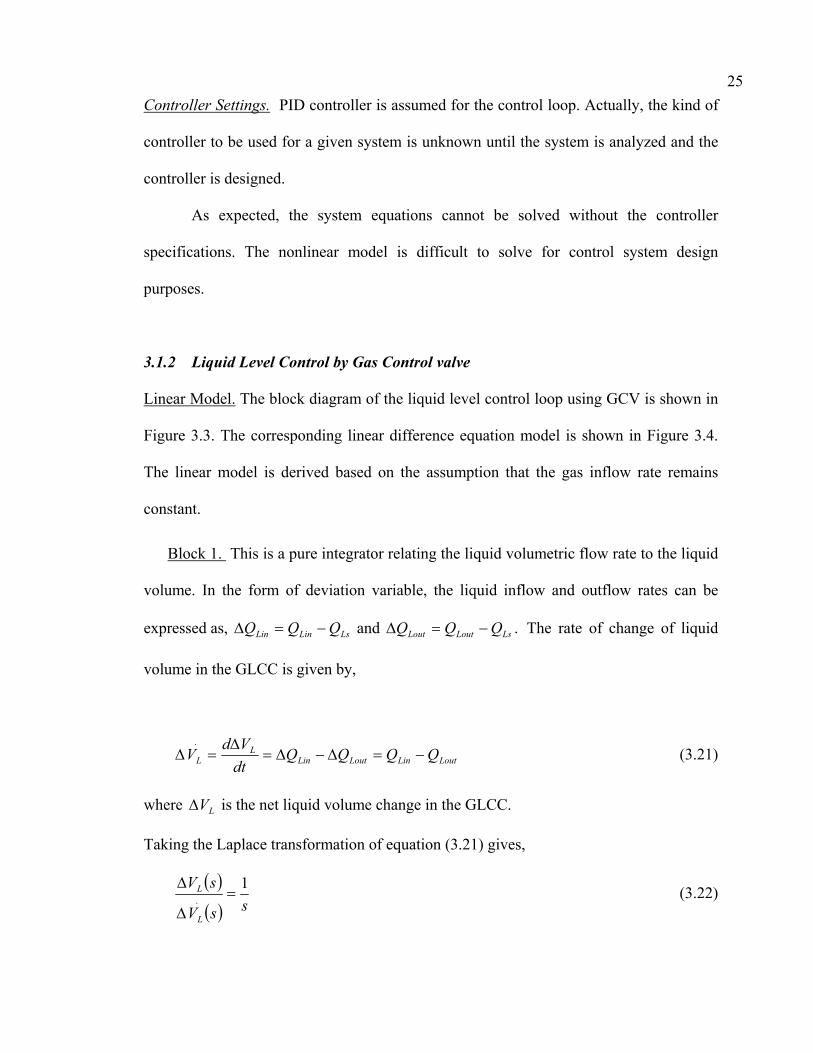
25Controller Settings. PID controller is assumed for the control loop. Actually, the kind of

controller to be used for a given system is unknown until the system is analyzed and the

controller is designed.

As expected, the system equations cannot be solved without the controller

specifications. The nonlinear model is difficult to solve for control system design

purposes.

3.1.2 Liquid Level Control by Gas Control valve

Linear Model. The block diagram of the liquid level control loop using GCV is shown in

Figure 3.3. The corresponding linear difference equation model is shown in Figure 3.4.

The linear model is derived based on the assumption that the gas inflow rate remains

constant.

Block 1. This is a pure integrator relating the liquid volumetric flow rate to the liquid

volume. In the form of deviation variable, the liquid inflow and outflow rates can be

expressed as, LsLinLin QQQ −=∆ and LsLoutLout QQQ −=∆ . The rate of change of liquid

volume in the GLCC is given by,

LoutLinLoutLinL

L QQQQdtVd

V −=∆−∆=∆

=∆.

(3.21)

where LV∆ is the net liquid volume change in the GLCC.

Taking the Laplace transformation of equation (3.21) gives,

( )( ) ssV

sV

L

L 1. =

∆

∆ (3.22)

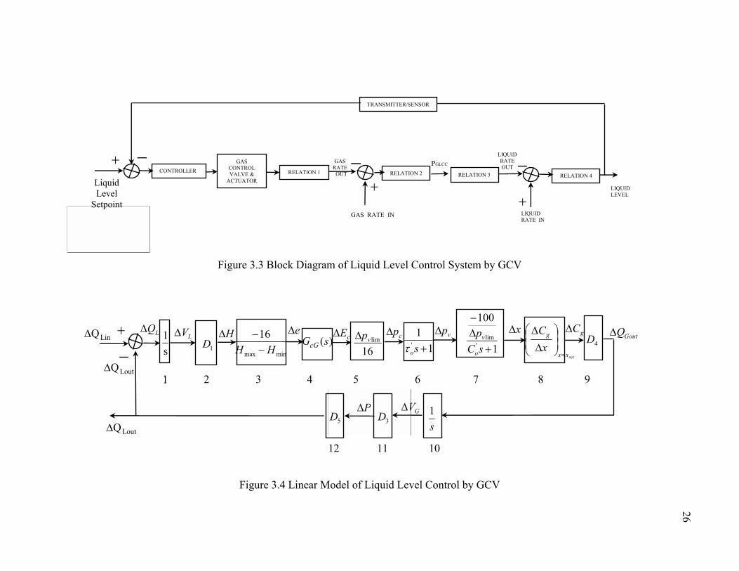
Figure 3.3 Block Diagram of Liquid Level Control System by GCV

Figure 3.4 Linear Model of Liquid Level Control by GCV

CONTROLLER

GAS RATE IN

TRANSMITTER/SENSOR

RELATION 4

+ GAS CONTROL VALVE &

ACTUATOR

GAS RATE OUT

LIQUID RATE IN

+

−− LIQUID RATE OUT

RELATION 2

PGLCC RELATION 1 RELATION 3

+

−LIQUID LEVEL

∆QLin+

−LV&∆1

s

LQ∆1DH∆ e∆ vp∆

1

100

'lim

+∆−

sCp

o

vx∆

setxx

g

xC

=

∆

∆4D

gC∆

∆QLout

11

' +soτcE∆

minmax

16HH −

− GoutQ∆)(sGcG

3DP∆

5D∆QLout

16limvp∆ cp∆

s1GV∆

1 2 3 4 5 6 7 8 9

10 11 12

1

Liquid Level

Setpoint

26

27

Block 2. This block presents the linear relationship between liquid level change and

the change of liquid volume in the GLCC. Using deviation variables in equation (3.15),

the liquid level can be expressed as, setHHH −=∆ . Substituting the deviation variables

and taking Laplace transform of equation (3.15) gives,

( )( ) 21

4dsV

sHDL π

=∆∆

= (3.23)

Block 3. This is the liquid level transmitter gain. As developed by Wang (2000),

based on the error signal and using deviation variables gives, )(16

minmax

HHH

e ∆−×−

=∆ .

Taking the Laplace transform yields,

( )( ) minmax

16HHsH

se−

−=

∆∆ (3.24)

Block 4. This is the unknown controller block, which needs to be specified in the

controller design. From Wang (2000), the general form of the mathematical description

for a PID controller is given by,

( )

++= st

stKsPID d

ic

11 (3.25)

or

( ) sksk

ksPID di

p ++= (3.26)

28

Block 5. This is the gain, which converts the controller output current signal (4-20

mA) to pneumatic pressure signal (typically 3-15 psi) to actuate the control valve.

( )( ) ( ) 16420

limminmax vvv

c

c pppsEsp ∆

=−−

=∆∆

(3.27)

Block 6. This is the transfer function for the pneumatic line delay.

11

' +≅

∆∆

spp

oc

v

τ (3.28)

Block 7. This is the transfer function for the control valve. As shown by Wang

(2000), taking derivative of the pneumatic control valve equation with respect to time

using deviation variables and taking the Laplace transform gives,

( )( ) 1

100

'lim

+

−

=∆∆

sCp

spsx

o

v

v

(3.29)

where minmaxlim vvv ppp −= . The negative sign comes from the reverse action of the

control valve.

29

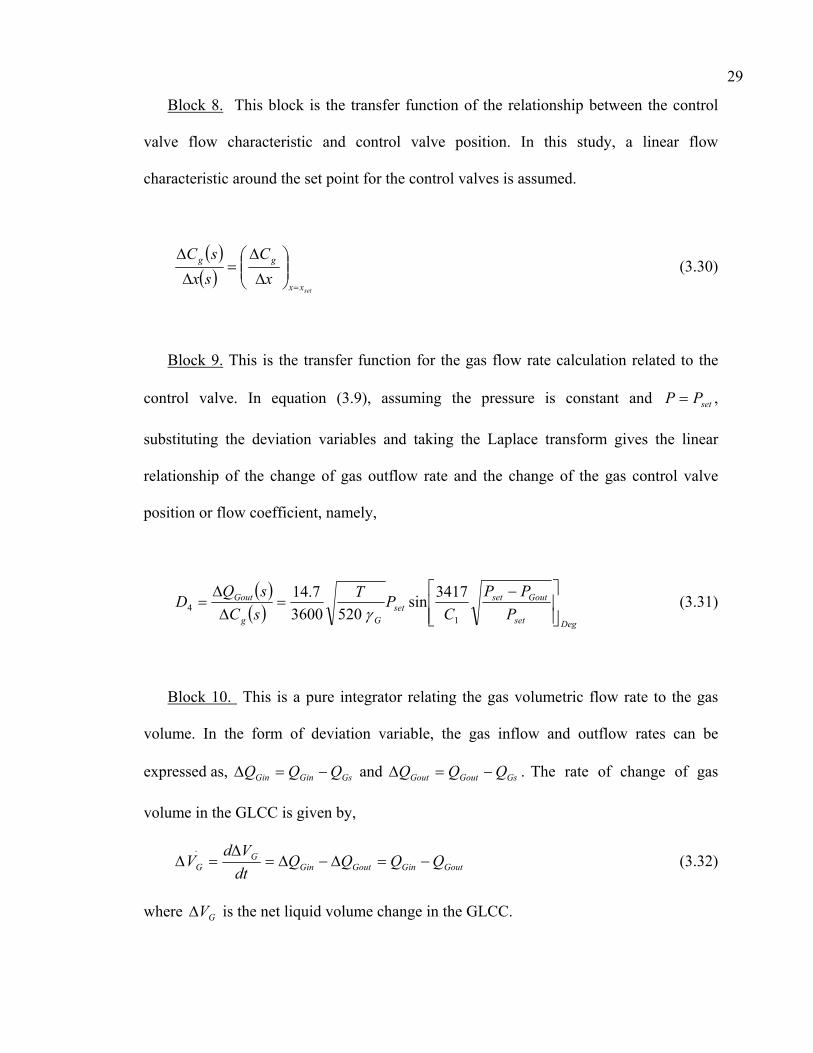
Block 8. This block is the transfer function of the relationship between the control

valve flow characteristic and control valve position. In this study, a linear flow

characteristic around the set point for the control valves is assumed.

( )( )

setxx

gg

xC

sxsC

=

∆

∆=

∆

∆ (3.30)

Block 9. This is the transfer function for the gas flow rate calculation related to the

control valve. In equation (3.9), assuming the pressure is constant and setPP = ,

substituting the deviation variables and taking the Laplace transform gives the linear

relationship of the change of gas outflow rate and the change of the gas control valve

position or flow coefficient, namely,

( )( )

Degset

Goutsetset

Gg

Gout

PPP

CPT

sCsQ

D

−=

∆∆

=1

43417sin

52036007.14

γ (3.31)

Block 10. This is a pure integrator relating the gas volumetric flow rate to the gas

volume. In the form of deviation variable, the gas inflow and outflow rates can be

expressed as, GsGinGin QQQ −=∆ and GsGoutGout QQQ −=∆ . The rate of change of gas

volume in the GLCC is given by,

GoutGinGoutGinG

G QQQQdtVd

V −=∆−∆=∆

=∆.

(3.32)

where GV∆ is the net liquid volume change in the GLCC.

30

Taking the Laplace transformation of equation (3.32) gives,

( )( ) ssV

sV

G

G 1. =

∆

∆ (3.33)

Block 11. This is the transfer function for the relationship between the GLCC

pressure and the net gas volume change in the GLCC. In equation (3.20), it is assumed

that the gas column volume GV is constant. This assumption is valid provided the liquid

level is controlled around the set point, which implies that the liquid outflow matches the

inflow. Also, it is assumed that the gas density to be constant (when the GLCC pressure

doesn’t change much). Using deviation variables and taking the Laplace transform gives,

( )s

DV

sP

G

13. ≅

∆

∆ (3.34)

where, ( )Gset

set

G VP

VsPD ≅

∆∆

=3 .

Block 12. This is another transfer function for the LCV liquid outflow rate

calculation. In this case, the control valve position or flow coefficient is assumed to be

constant at the initial position corresponding to the set point flow conditions. The liquid

outflow is assumed to be driven by the GLCC pressure alone. Using deviation variables

and taking the Laplace transform of equation (3.3) gives,

( )( ) LoutsetL

vsetLout

PPC

sPsQ

D−

=∆

∆=

121002228.0

5 γ (3.35)

31

Controller Design: The open loop transfer function can be obtained from the linear model

of liquid level control by GCV that is given by,

( ) ( ) ( ))1)(1( ''2 ++

=ssCs

KsGsGsH

oo

scG τ

(3.36)

where:

)(sH - feed back path transfer function

)(sG - feed forward path transfer function

)(sGcG - controller transfer function, need to be determined from the design.

sK - the system gain, which is given by,

setxx

g

v

vs x

Cp

pHH

DDDDK=

∆

∆

∆−

∆

−

−=

lim

lim

minmax5431

10016

16 (3.37)

Further details on the controller design and additional calculations can be found in the

work of Wang (2000).

3.1.3 GLCC Gas Carry-Under

Due to the complex nature of the GLCC dynamic system, a simple method is

required to study the gas carry-under in the liquid leg. Marrelli, et al. (2000) developed a

correlation to predict the gas void fraction in the GLCC underflow based on the in-situ

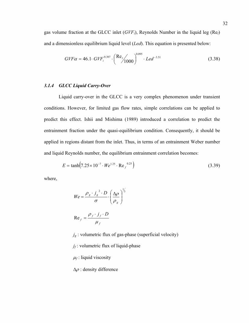
32

gas volume fraction at the GLCC inlet (GVFi), Reynolds Number in the liquid leg (Rel)

and a dimensionless equilibrium liquid level (Led). This equation is presented below:

51.3095.0

307.0

1000Re1.46 −⋅

⋅⋅= LedGVFGVF l

iα (3.38)

3.1.4 GLCC Liquid Carry-Over

Liquid carry-over in the GLCC is a very complex phenomenon under transient

conditions. However, for limited gas flow rates, simple correlations can be applied to

predict this effect. Ishii and Mishima (1989) introduced a correlation to predict the

entrainment fraction under the quasi-equilibrium condition. Consequently, it should be

applied in regions distant from the inlet. Thus, in terms of an entrainment Weber number

and liquid Reynolds number, the equilibrium entrainment correlation becomes:

( )25.025.17 Re1025.7tanh fWeE ⋅⋅×= − (3.39)

where,

3

12

∆⋅

⋅⋅=

g

gg DjWe

ρρ

σρ

f

fff

Djµ

ρ ⋅⋅=Re

jg : volumetric flux of gas-phase (superficial velocity)

jf : volumetric flux of liquid-phase

µf : liquid viscosity

∆ρ : density difference

33

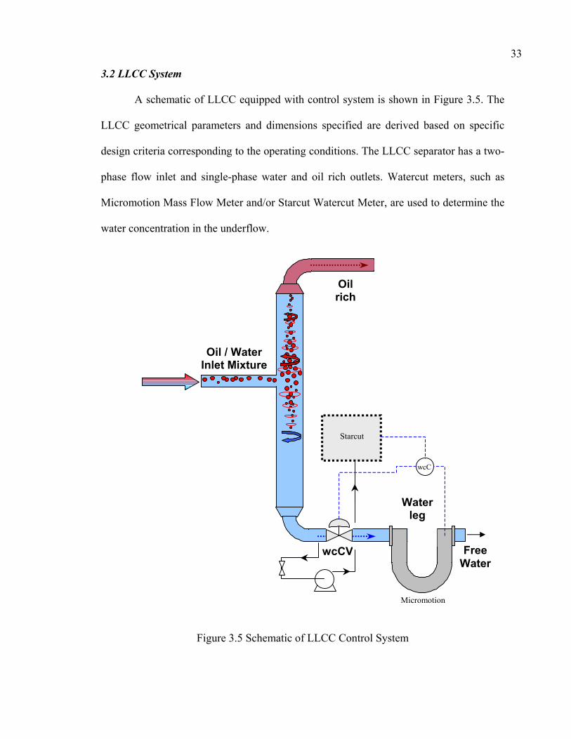
3.2 LLCC System

A schematic of LLCC equipped with control system is shown in Figure 3.5. The

LLCC geometrical parameters and dimensions specified are derived based on specific

design criteria corresponding to the operating conditions. The LLCC separator has a two-

phase flow inlet and single-phase water and oil rich outlets. Watercut meters, such as

Micromotion Mass Flow Meter and/or Starcut Watercut Meter, are used to determine the

water concentration in the underflow.

Starcut

Micromotion

wcC

wcCV

Oil rich

Oil / WaterInlet Mixture

Water leg

Figure 3.5 Schematic of LLCC Control System

Free Water

34

The actuating signal from the watercut meter is sent to the controller to control the

position of the control valve, which is mounted in the LLCC underflow line. The

operation of LLCC strongly depends upon the split of inlet flow rates. Split Ratio, S.R, is

an important parameter used in this study to quantify the performance of LLCC. It is the

ratio of the underflow rate to the total inlet flow rate, as given below:

S.R = Qin

Qunderflow × 100 % (3.40)

The main objective of using a LLCC compact separator is to provide an effective

alternative for oil-water separation in the form of a free-water knockout device. Hence,

there exists an optimal split ratio that depends upon the LLCC inlet flow conditions.

Optimal Split Ratio is defined as that particular split in which maximum underflow in

LLCC is obtained and at the same time maintaining clear water in the underflow.

However, the inlet water and oil flow rate fluctuations will cause the watercut in the

underflow to fluctuate during operation. These dynamics affect the performance of the

LLCC since watercut at the inlet is an indirect parameter of the optimal split ratio.

Therefore, the objective of the control system is to maintain the optimal split ratio for

different inlet oil and water flow rates.

A schematic of the control strategy developed in this study is shown in Figure 3.6.

The sensor/transmitter (Micromotion Mass Flow Meter and/or Starcut Watercut Meter)

measure the control parameter, in this case the underflow watercut, directly and converts

the watercut signal into current signal in the range of 4-20 mA. This signal is compared

to the watercut set point and the error signal is sent to the controller. The controller

35

output is sent to the control valve in the form of pneumatic actuating pressure signal to

control the valve position accordingly.

Liquid Underflow Flowrate

Watercut Setpoint Downstream

Controller Pneumatic

Line Water

Control Valve Relation

1 2 3,4,5,6 7,8

Watercut Sensor/Transmitter

Actual Watercut

Inlet Oil Flowrate

Inlet Water Flowrate

+

- +

-

Figure 3.6 Schematic of LLCC Control Loop

Design Elements of the Control System

The sequence of procedure followed for LLCC control system design and analysis

is discussed below in detail.

a) Control Objectives:

The central element in any control configuration is the process that needs to be

controlled. Thus, the control objectives for LLCC control are two-fold:

i) obtain clear water in the underflow and

ii) maximize the amount of water that can be separated.

b) Selection of Measurements:

Some means to monitoring the performance of a process is needed in order to

achieve the control objectives. This is done, by measuring the values of certain process

variables that represent the control objectives. In this case, the variable that is used to

monitor the performance of LLCC is watercut in the underflow.

36

c) Selection of Manipulated Variables:

Manipulated variables are those that can be used to control a process. In this case,

position of control valve is the manipulated variable.

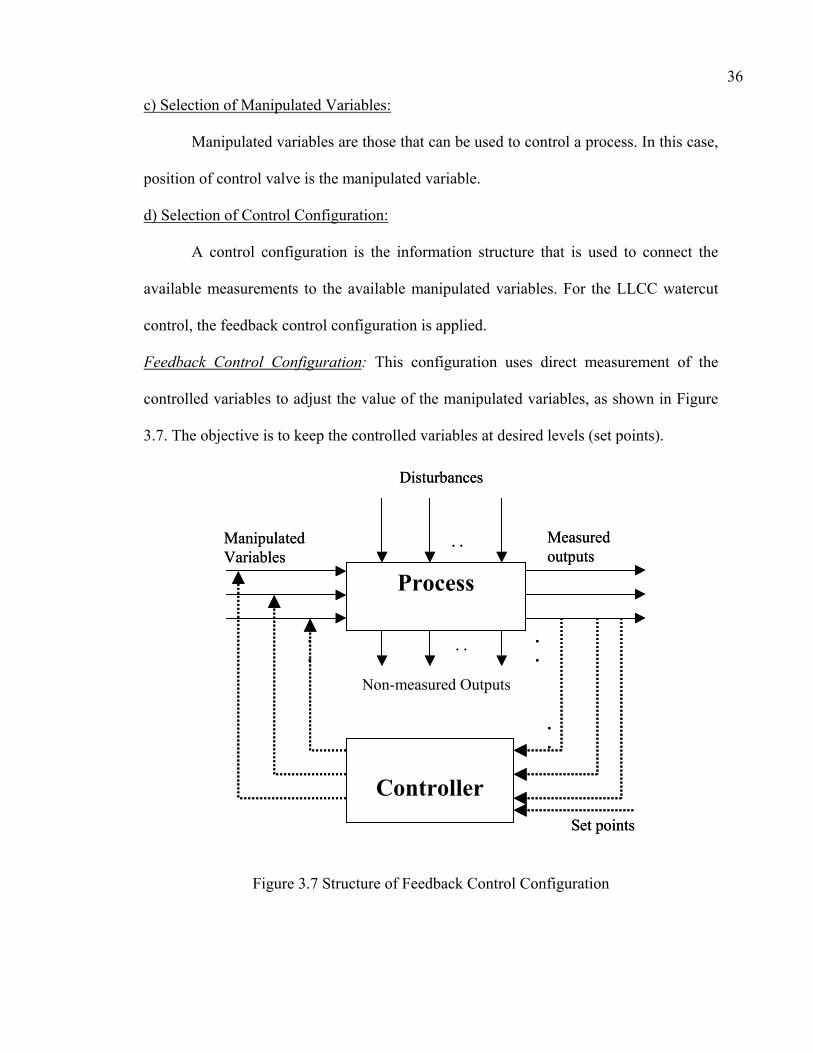
d) Selection of Control Configuration:

A control configuration is the information structure that is used to connect the

available measurements to the available manipulated variables. For the LLCC watercut

control, the feedback control configuration is applied.

Feedback Control Configuration: This configuration uses direct measurement of the

controlled variables to adjust the value of the manipulated variables, as shown in Figure

3.7. The objective is to keep the controlled variables at desired levels (set points).

.

.. .

Measured outputs

Unmeasured Outputs

Manipulated Variables

Disturbances

.

.

Process

. .

ControllerSet points

.

...

. .

Measured outputs

Unmeasured Outputs

Manipulated Variables

Disturbances

.

.

Process

. .

Process

. .

ControllerSet points

.

.

Figure 3.7 Structure of Feedback Control Configuration

Non-measured Outputs

37

3.2.1 Linear Model for LLCC Control

The main reason for developing a linear model is to approximate the dynamic

behavior of a nonlinear system in the neighborhood of specified operating conditions.

This approach, in principle, is always feasible and is widely used in the study of process

dynamics and design of control systems. The main advantages are as follows:

• Analytical solutions can be obtained for linear systems. It helps to obtain a

complete and general picture of system’s behavior.

• Most significant developments towards the design of effective control

systems are available for linear systems.

The block diagram of the watercut control loop using a control valve in the water

leg is shown earlier in Figure 3.6. The corresponding linear model is shown in Figure 3.8.

The transfer functions given in the blocks are stepwise mathematical descriptions of the

physical subsystems in Laplace domain. The transfer functions are related to deviation

variables instead of actual variables. A deviation variable is the deviation of a variable

from its steady-state or set point value, denoted by a preceding ∆. The reason for using

deviation variables is that the ratio of the output to the input of a block can be expressed

linearly. This is done assuming that the real controlled variable is at the set point value

from steady state conditions.

Figure 3.8 Linear Model of LLCC Control Loop

1. Feedback Controller 5. C.V Characteristics 2. Pneumatic Line Gain 6. Underflow Calculation 3. Actuator Delay 7,8. Watercut Calculation 4. C.V. Response Time 9. Transmitter Gain

− 1Dsetxxx

vC

=

∆∆

11+soτ

)s(1cG

1 2 3 4 5 6

vp∆cp∆ uQ∆cE∆ x∆ vC∆

6

inQ∆

minmax ..16

CWCW −

Qo∆

inQ∆1 C

7 8

RS.1 ∆− CW .∆+

1p/100 vlim

+∆sCo

e∆

∆

16limvp

38

39

Block 1:

This is the unknown controller block that needs to be determined from the

controller design. As reported by Mathiravedu (2001), the transfer function for a PI

controller is given by,

( )

+=

st11KsPIi

c (3.41)

or

( )sk

ksPI ip += (3.42)

Block 2:

This is the gain, which converts the controller output current signal (4-20 mA) to

pneumatic pressure signal (typically 3-15 psig) to actuate the control valve.

≅∆∆

)()(

sEsp

c

c

( )420minmax

−− vv pp

=16

limvp∆ (3.43)

Block 3:

This is the transfer function of pneumatic line delay.

1

1)()(

+≅

∆∆

sspsp

oc

v

τ (3.44)

Block 4:

This is the transfer function for the control valve. Mathiravedu (2001) verified

that taking derivative of the pneumatic control valve equation with respect to time using

deviation variables and taking the Laplace transform gives,

( )( ) 1sC

p100

spsx

o

v

v +=

∆∆ lim (3.45)

40

where, minmaxlim vvv ppp −= (12 psig in this study)

Block 5:

As presented before, this block denotes the transfer function of the relationship

between the control valve flow characteristics and control valve position. In this study, a

linear flow characteristic around the set point is assumed.

( )( )

setxx

vv

xC

sxsC

=

∆∆

=∆∆

(3.46)

Block 6:

This is the transfer function of the liquid flow rate calculation for the control

valve. Assuming that the pressure drop across the control valve is constant, the liquid

flow rate is only a function of flow coefficient. Taking derivative of equation (3.3), using

deviation variables and taking the Laplace transform gives,

( )( ) L

LCV1

γ∆P

0.002228sv∆C

su∆Q D == (3.47)

Block 7:

This is the transfer function that converts the overflow rate to the split ratio.

Recall that the split ratio is defined as the ratio of the underflow rate to the total inlet flow

rate, namely,

S.R. = in

u

QQ and dS.R. =

in

u

dQdQ

Using deviation variables,

41

( ) ( )( )sQsQsRS

in

u

∆∆

=∆ .

1- ( ) =∆ sRS. 1- ( )( )sQsQ

in

u

∆∆

1- ( ) =∆ sRS. ( ) ( )( )sQ

sQsQ

in

uin

∆∆−∆

1- ( ) ( )( )sQsQsRS

in

o

∆∆

=∆ .

( )

( ) ( )sQ1

sQsRS1

ino ∆=

∆

∆− . (3.48)

Block 8:

This is the transfer function that converts the split ratio to the underflow watercut.

The conversion value is obtained from the graph plotted using the experimental data.

Using deviation variables, this transfer function is given by:

Slope (C) = ( )( ) =− sRS1d

sCdW).(

.. ( )( )sRS1sCW

...

∆−

∆ (3.49)

Block 9:

This is the watercut sensor/transmitter gain. As confirmed by Mathiravedu (2001),

using deviation variables in the controller error signal equation and taking the Laplace

transform gives,

42

( )( ) minmax ....

16. CWCWsCW

se−

=∆∆ (3.50)

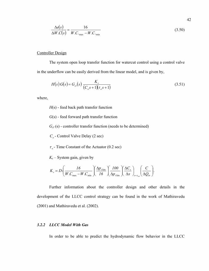
Controller Design

The system open loop transfer function for watercut control using a control valve

in the underflow can be easily derived from the linear model, and is given by,

( ) ( ) ( ) ( )( )11 ++=

ssCK

sGsGsHoo

scl τ

(3.51)

where,

H(s) - feed back path transfer function

G(s) - feed forward path transfer function

Gcl (s) - controller transfer function (needs to be determined)

oC - Control Valve Delay (2 sec)

oτ - Time Constant of the Actuator (0.2 sec)

Ks – System gain, given by

∆

∆∆

∆

∆

−

== inxx

v

v

v1s Q

Cx

Cp100

16p

CWCW16DK

setlim

lim

minmax ...

Further information about the controller design and other details in the

development of the LLCC control strategy can be found in the work of Mathiravedu

(2001) and Mathiravedu et al. (2002).

3.2.2 LLCC Model With Gas

In order to be able to predict the hydrodynamic flow behavior in the LLCC

43

operating with small amount of gas, it is important to understand the associated physical

phenomenon. Little amount of gas into the system does not affect the inlet flow patterns

and behavior of the flow in the nozzle. However, when the fluids reach the LLCC body,

and as a result of the vortex forces produced by the swirling phenomenon, gas is attached

to the oil and the water phases. The gas gets attached mainly to the oil, reducing its

density. This causes lower drag between the oil droplets and the continuous water-phase,

causing an improvement in the separation efficiency. The water density is also affected,

because some part of the gas is attached to the water phase.

At the LLCC inlet, the gas phase splits, whereby part of the gas flows upwards

into the upper LLCC part and the other part flows downwards into the lower LLCC part.

Using experimental data, Contreras (2002) developed correlations for the gas void

fraction in the oil phase (αG(o)) and in the water phase (αG(w)) in the underflow of the

LLCC, as follows:

FglGVFFglVslVsg

VsgoG =

+=)(α (3.52)

)1()1()( FglGVFFglVslVsg

VsgwG −=−

+=α (3.53)

Next the densities of the oil and water phases (with the attached gas) are,

respectively:

)()(mod )1( oGgoGoo αραρρ +−= (3.54)

)()(mod )1( wGgwGww αραρρ +−= (3.55)

The GVF is the inlet gas void fraction and Fgl is a factor determined

44

experimentally, which depends on the inlet watercut, as shown in Table 3.1.

This model is able to describe the phenomenon when the LLCC works with small

amount of gas, up to the maximum efficiency point of the LLCC. Beyond this point, a

behavior reversal occurs and the LLCC efficiency decreases. The LLCC model with gas

does not describe this reversal process. However, the description of this process is not

critical, because the LLCC under these conditions is not efficient.

Table 3.1 Values of Empirical Factor, Fgl

Inlet Watercut % Fgl

60-75 0.58 75-85 0.54 >85 0.53

GVF Effect on LLCC Performance:

The effect of the gas void fraction on the LLCC performance was studied by

Contreras (2002), reporting results like those shown in Figure 3.9. This demonstrates that

for a fixed watercut introduced to the LLCC, the presence of gas improves the separation

efficiency of the equipment until reaching a maximum point where the effect of

additional gas drops the efficiency until the stage where the separator performance

deteriorates drastically.

Based on the experimental data a correlation is proposed in order to capture this

phenomenon. This correlation establishes the relationship between the underflow

watercut and the split ratio for different GVF values.

( )%exp% SRBAWC ⋅⋅= (3.56)

where A & B are functions of the GVF%, given by

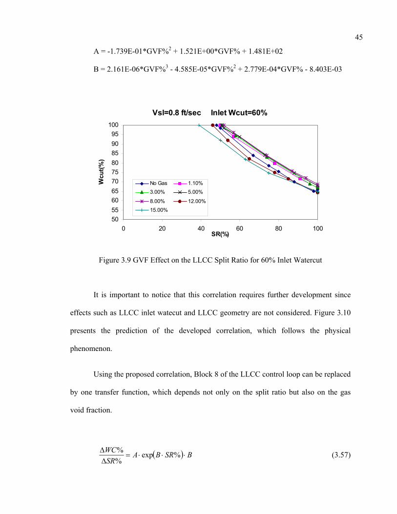
45

A = -1.739E-01*GVF%2 + 1.521E+00*GVF% + 1.481E+02

B = 2.161E-06*GVF%3 - 4.585E-05*GVF%2 + 2.779E-04*GVF% - 8.403E-03

Vsl=0.8 ft/sec Inlet Wcut=60%

50556065707580859095

100

0 20 40 60 80 100SR(%)

Wcu

t(%)

No Gas 1.10%3.00% 5.00%

8.00% 12.00%15.00%

Figure 3.9 GVF Effect on the LLCC Split Ratio for 60% Inlet Watercut

It is important to notice that this correlation requires further development since

effects such as LLCC inlet watecut and LLCC geometry are not considered. Figure 3.10

presents the prediction of the developed correlation, which follows the physical

phenomenon.

Using the proposed correlation, Block 8 of the LLCC control loop can be replaced

by one transfer function, which depends not only on the split ratio but also on the gas

void fraction.

( ) BSRBASRWC

⋅⋅⋅=∆∆ %exp

%% (3.57)

46

SR% in LLCCcorrelation prediction

0

10

20

30

40

50

60

70

0 5 10 15 20

GVF%

SR%

SR%

Figure 3.10 Prediction of LLCC Split Ratio as a Function of the GVF

for 60% Inlet Watercut

The values obtained using equation 3.56 are between 0.4 and 1.0. Although this

correlation was developed for LLCC inlet watercut of 60%, the correction for the

watercut to split ratio gain for other inlet watercuts should not make a significant

difference in the analysis of the system.

GVF Effect on LLCC Control System Stability:

As a consequence of the modification in the LLCC control loop due to the new

split ratio to watercut transfer function (equation 3.56), the root-locus stability map

should be re-evaluated in order to make sure that the control strategy developed is still

stable in the presence of gas. For split ratios from 30 to 100% and for GVF from 0 to

17% the value of this transfer function (gain) oscillates between 0.9672 and 0.4154. The

47

result of the root locus for this range is shown in Figure 3.11 where the arrows indicate

the trajectory covered by the different values.

Figure 3.11 Root Locus Plot for LLCC with Gas

It is clear that for the range studied, the system remains stable in the presence of

gas and under the 40% overshoot region.

3.3 GLCC / LLCC System

Founded on the developments through the years of the GLCC and LLCC

technologies, the next step is to combine both separators as a three-phase separation

system.

48

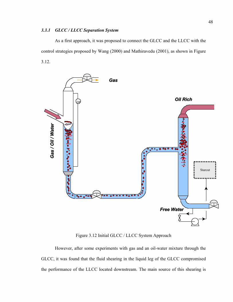
3.3.1 GLCC / LLCC Separation System

As a first approach, it was proposed to connect the GLCC and the LLCC with the

control strategies proposed by Wang (2000) and Mathiravedu (2001), as shown in Figure

3.12.

Starcut

DP

Gas

/ O

il / W

ater

Gas

/ O

il / W

ater

GasGas

Free WaterFree Water

Oil RichOil Rich

Starcut

DP

Starcut

DPDP

Gas

/ O

il / W

ater

Gas

/ O

il / W

ater

GasGas

Free WaterFree Water

Oil RichOil Rich

Figure 3.12 Initial GLCC / LLCC System Approach

However, after some experiments with gas and an oil-water mixture through the

GLCC, it was found that the fluid shearing in the liquid leg of the GLCC compromised

the performance of the LLCC located downstream. The main source of this shearing is

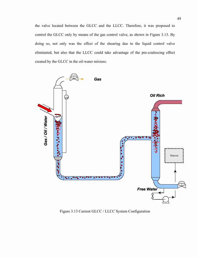
49

the valve located between the GLCC and the LLCC. Therefore, it was proposed to

control the GLCC only by means of the gas control valve, as shown in Figure 3.13. By

doing so, not only was the effect of the shearing due to the liquid control valve

eliminated, but also that the LLCC could take advantage of the pre-coalescing effect

created by the GLCC in the oil-water mixture.

Starcut

DP

Gas

/ O

il / W

ater

Gas

/ O

il / W

ater

GasGas

Free WaterFree Water

Oil RichOil Rich

Starcut

DP

Starcut

DPDP

Gas

/ O

il / W

ater

Gas

/ O

il / W

ater

GasGas

Free WaterFree Water

Oil RichOil Rich

Figure 3.13 Current GLCC / LLCC System Configuration

50

3.3.2 Droplet Size Behavior Through Control Valves

As explained before, an accessory such as a valve could produce a dramatic

change in the two-phase mixture flowing from the GLCC to the LLCC, even to the point

of creating an emulsion that is impossible to separate. Thus, previous research done in the

area of emulsion formation in valves and orifice plates is applied to this particular case.

Janssen (2001) studied this problem based on the work from Hinze (1955) deriving an

expression for the maximum droplet diameter:

525

3

53

max

−⋅

⋅= ερσ

ccritWed (3.58)

where Wecrit is the Weber number of the maximum stable droplet:

+

⋅⋅

=2

324

2

c

dcritWe

ρρ

π (3.59)

The average amount of energy that is being dissipated per time and mass unit can be

estimated by:

dis

operm

LUP

⋅

⋅∆≈

ρε (3.60)

where,

Uo : average fluid velocity through the restriction

∆Pperm : permanent pressure drop

Ldis : length of the dissipation zone

Using this model and equation 3.3, which describes the flow through a control

valve, one can analyze how the closing-opening action of a liquid control valve will

affect the oil droplets dispersed in water.

51

For a perturbation of ∆Qgas = -0.5 ft3/s and ∆Qliquid = 0.06 ft3/s, using the

differential model implemented by Wang (2000) with the purpose of controlling the

liquid level in the GLCC, the results of the valve action on the droplet size distribution

can be observed in Figures 3.14 and 3.15. For the given perturbation, LCV position and

pressure drop are plotted as a function of time in Figure 3.14 and the droplet size is

plotted as a function of time in Figure 3.15.

LCV position and Pressure Dropthrough LCV

0.0

10.0

20.0

30.0

40.0

50.0

0.0 5.0 10.0 15.0 20.0 25.0 30.0

t (s)

LCV

posi

tion

(%)

0.100.150.200.250.300.350.400.450.500.55

DP

(psi

d)

LCV

DP

Figure 3.14 LCV Position and Pressure Drop in Control Valve

While the control valve is closing, the shearing applied to the oil-water mixture

flowing through the valve is increased. As a consequence, the droplet size of the oil

dispersed in water is reduced up to 60% of its original size, as shown in Figure 3.15.

Hence, it is desirable to eliminate the usage of LCV between the GLCC and the LLCC.

)

52

Droplet Size after a Control Valve

300

350

400

450

500

550

600

650

0.0 5.0 10.0 15.0 20.0 25.0 30.0

t (s)

Dro

plet

Siz

e (m

icro

ns)

dpmax

Figure 3.15 Maximum Droplet Size Downstream of a Control Valve

3.3.3 Pressure Losses Between GLCC and LLCC

Calculation of the pressure losses of a two-phase mixture can be a complex task,

depending on the model used. Considering the pressure losses between the GLCC and the

LLCC in the dynamic models, a simplification has been made. A non-slip homogeneous

flow of two incompressible liquids (oil and water) is assumed. This led to simplifications

to use average properties, such as density and viscosity, for the mixture. Therefore, based

on the continuity and momentum equations the pressure losses can be computed as

shown below:

( ) ( ) 0=⋅⋅∂∂

+⋅∂∂

mmm VAx

At

ρρ (3.61)

obtaining, 0=∂∂

xVm

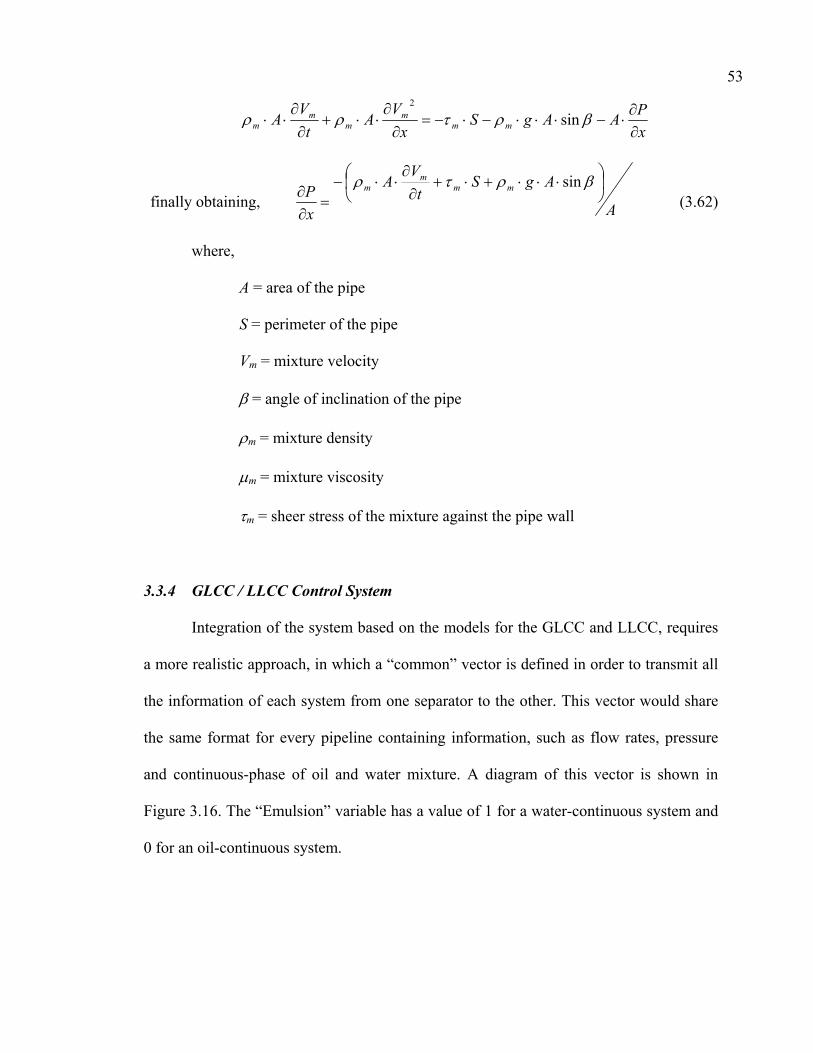
53

xPAAgS

xV

At

VA mm

mm

mm ∂

∂⋅−⋅⋅⋅−⋅−=

∂∂⋅⋅+

∂∂⋅⋅ βρτρρ sin

2

finally obtaining, A

AgSt

VA

xP mm

mm

⋅⋅⋅+⋅+

∂∂⋅⋅−

=∂∂

βρτρ sin (3.62)

where,

A = area of the pipe

S = perimeter of the pipe

Vm = mixture velocity

β = angle of inclination of the pipe

ρm = mixture density

µm = mixture viscosity

τm = sheer stress of the mixture against the pipe wall

3.3.4 GLCC / LLCC Control System

Integration of the system based on the models for the GLCC and LLCC, requires

a more realistic approach, in which a “common” vector is defined in order to transmit all

the information of each system from one separator to the other. This vector would share

the same format for every pipeline containing information, such as flow rates, pressure

and continuous-phase of oil and water mixture. A diagram of this vector is shown in

Figure 3.16. The “Emulsion” variable has a value of 1 for a water-continuous system and

0 for an oil-continuous system.

54

QoilQwaterQgasQsolidsEmulsionPressure

QoilQwaterQgasQsolidsEmulsionPressure

Figure 3.16 Common Vector for Each Pipeline

Simulator Development

Since the method of describing the system as real as possible is desired, the

approach of expressing the results of the simulations in terms of absolute values is easier

to understand and more likely to capture the process performance for situations such as

different set points, start-up operations and other transient circumstances. The control

models developed previously by Wang (2000), and Mathiravedu (2001) were expressed

in terms of deviation variables, which require converting the results from the differential

models into absolute values. The absolute (realistic) input vector is also, required to be

expressed in appropriate terms that the differential models would recognize.

The simulator was built using Matlab/Simulink® organized in modules and

subsystems, as shown below.

Simulator Structure:

• Input vector module

• Properties vector module

• GLCC module

- GLCC control subsystem

- GLCC liquid carry-over subsystem

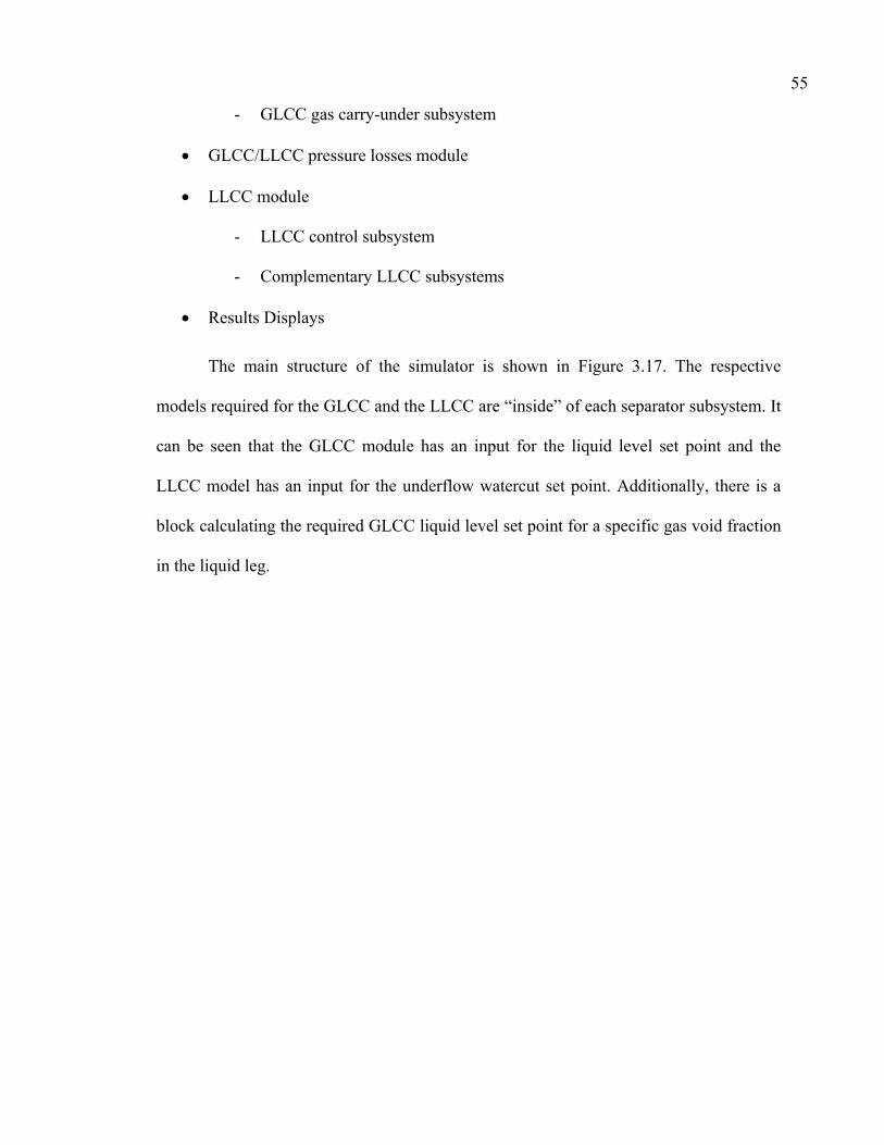
55

- GLCC gas carry-under subsystem

• GLCC/LLCC pressure losses module

• LLCC module

- LLCC control subsystem

- Complementary LLCC subsystems

• Results Displays

The main structure of the simulator is shown in Figure 3.17. The respective

models required for the GLCC and the LLCC are “inside” of each separator subsystem. It

can be seen that the GLCC module has an input for the liquid level set point and the

LLCC model has an input for the underflow watercut set point. Additionally, there is a

block calculating the required GLCC liquid level set point for a specific gas void fraction

in the liquid leg.

+ Figure 3.17 GLCC / LLCC System Simulator

56

57

• Input vector module

In this module, all the input variables can be modified in order to study the

performance of a system under different perturbations. The step functions can be

replaced by other functions to reproduce a desired pattern. This module is shown in

Figure 3.18.

Figure 3.18 Input Vector Module

58

• Properties vector module

This vector shown in Figure 3.19, accounts for all the different densities of the

fluids to be considered. In this case, the input is the specific gravity.

Figure 3.19 Properties Vector Module

• GLCC module

As shown in Figure 3.20, this module contains the GLCC liquid level control, the

gas carry-under and the liquid carry-over subsystems.

Figure 3.20 GLCC Model Subsystem

59

- GLCC control subsystem

Figure 3.21 GLCC Level Control Subsystem

60

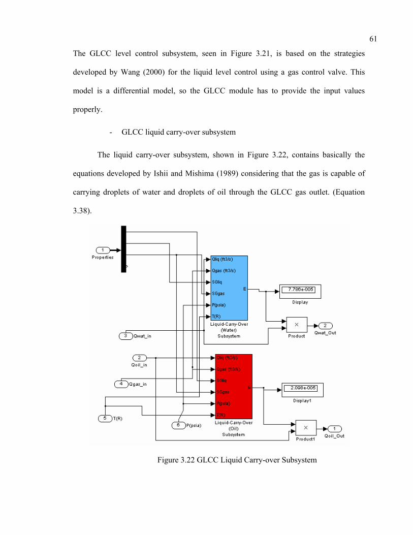
61

The GLCC level control subsystem, seen in Figure 3.21, is based on the strategies

developed by Wang (2000) for the liquid level control using a gas control valve. This

model is a differential model, so the GLCC module has to provide the input values

properly.

- GLCC liquid carry-over subsystem

The liquid carry-over subsystem, shown in Figure 3.22, contains basically the

equations developed by Ishii and Mishima (1989) considering that the gas is capable of

carrying droplets of water and droplets of oil through the GLCC gas outlet. (Equation

3.38).

Figure 3.22 GLCC Liquid Carry-over Subsystem

62

- GLCC gas carry-under subsystem

The GLCC Gas Carry-Under subsystem displayed in Figure 3.23 calculates the

gas void fraction in the liquid leg of the GLCC based on the work presented by Marrelli

et al. (2000). (Equation 3.37).

Figure 3.23 GLCC Gas Carry-under Subsystem

• GLCC/LLCC pressure losses module

The pressure losses module, shown in Figure 3.24, represents the calculation of

the frictional losses based on the momentum equation for the mixture flowing from the

GLCC through the liquid leg into the LLCC.

63

Figure 3.24 GLCC/LLCC Pressure Losses Subsystem

• LLCC module

The LLCC module represented in Figure 3.25 handles the watercut control

subsystem, and the LLCC auxiliary subsystems such as the LLCC Split ratio GVF

dependant subsystem, gas in LLCC underflow subsystem and continuous-phase

detectors. The LLCC module not only integrates these subsystems, but also provides the

input to the watercut control subsystem.

Figure 3.25 LLCC Model Subsystem

64

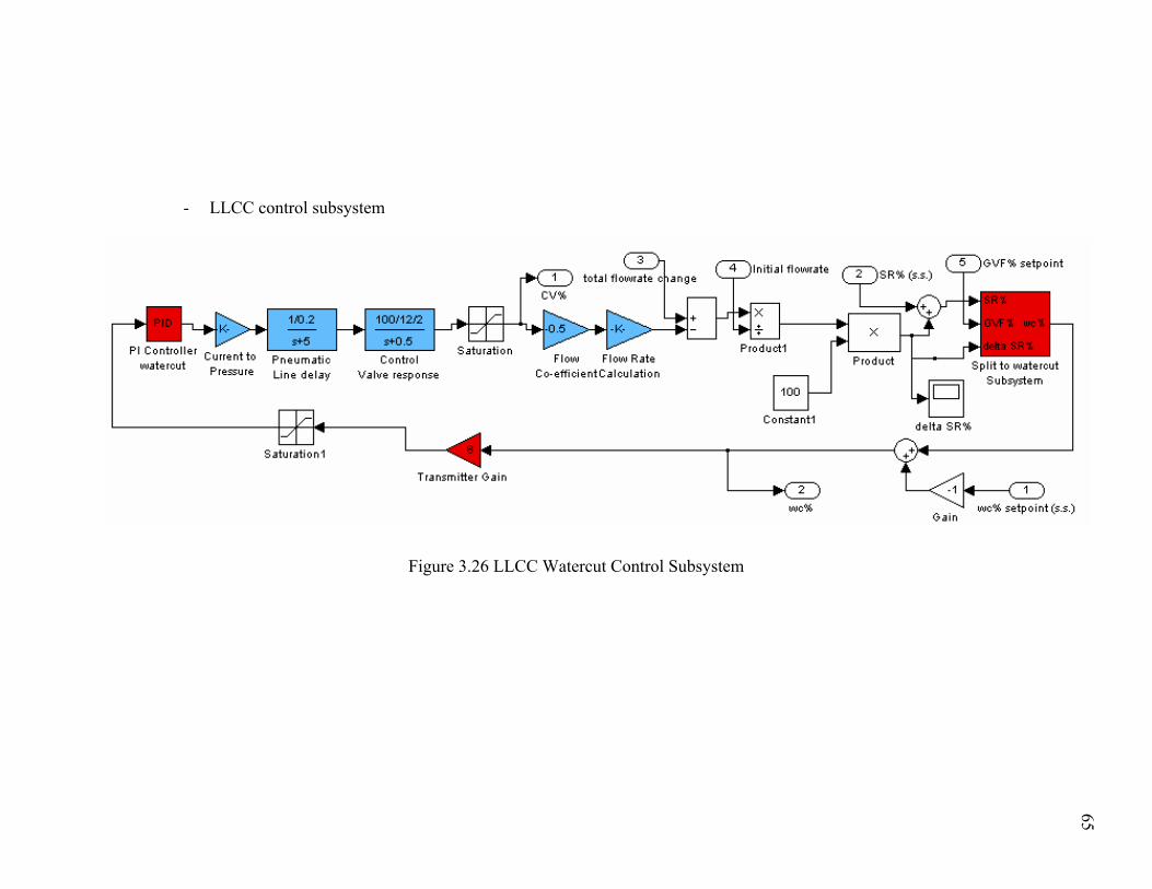
- LLCC control subsystem

Figure 3.26 LLCC Watercut Control Subsystem

65

66

The LLCC control subsystem shown in Figure 3.26 is based on the work of

Mathiravedu (2001). The split ratio to watercut block is modified to account for the effect

of gas on the LLCC performance.

- Complementary LLCC subsystems

The LLCC split ratio to watercut subsystem shown in Figure 3.27 incorporates the

correlation proposed in this study to capture the separation efficiencies as function of gas

void fraction.

Figure 3.27 LLCC Split Ratio to watercut Subsystem

The gas in LLCC underflow subsystem displayed in Figure 3.28 contains the

correlations developed by Contreras (2002) with the purpose of quantifying the amount

of gas in the underflow of the LLCC.

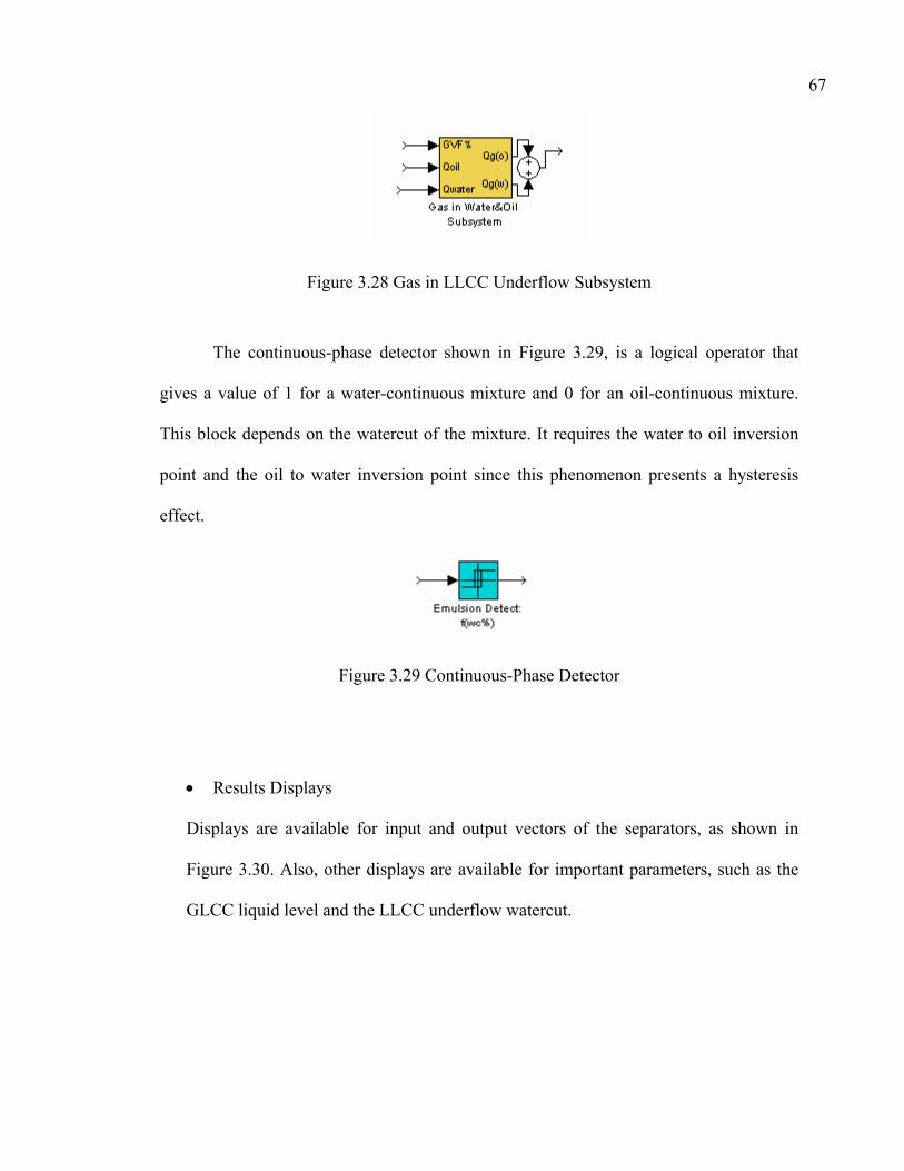
67

Figure 3.28 Gas in LLCC Underflow Subsystem

The continuous-phase detector shown in Figure 3.29, is a logical operator that

gives a value of 1 for a water-continuous mixture and 0 for an oil-continuous mixture.

This block depends on the watercut of the mixture. It requires the water to oil inversion

point and the oil to water inversion point since this phenomenon presents a hysteresis

effect.

Figure 3.29 Continuous-Phase Detector

• Results Displays

Displays are available for input and output vectors of the separators, as shown in

Figure 3.30. Also, other displays are available for important parameters, such as the

GLCC liquid level and the LLCC underflow watercut.

68

GLCC inlet LLCC underflow LLCC overflow

Figure 3.30 GLCC/LLCC Simulator Results Displays

Simulation Results

With the intention of testing the models for the GLCC and the LLCC in absolute

values, three kind of simulations were run, including:

i) GLCC/LLCC system for different GLCC liquid level setpoints

ii) GLCC/LLCC system for different LLCC underflow watercut setpoints

iii) GLCC/LLCC system for different inlet flowrates

The controller settings used for all these simulations, as defined below, are

specified in Table 3.2.

pKP =i

pi K

KT =p

dd K

KT = (3.63, 3.64, 3.65)

69

Table 3.2 PID Settings for GLCC and LLCC Controllers During Simulations

GLCC Settings LLCC Settings P 0.1100 Kp 0.1100 P 1.6500 Kp 1.6500

I (s-1) 0.0300 Ti (min) 0.0611 I (s-1) 0.9500 Ti (min) 0.0289 D (s) 0.1000 Td (min) 0.0152 D (s) 0.0000 Td (min) 0.0000

i) GLCC/LLCC system for different GLCC liquid level setpoints:

The main purpose of this simulation is to see the performance of the GLCC liquid

level control for different liquid level setpoints and its effects on the downstream system.

For this reason, a set of different liquid level setpoints was chosen as the input to the

system while keeping the input flowrates constant. These perturbations are shown in

Figure 3.31.

Liq. Level setpoint in GLCC

0.00.51.01.52.0

2.53.03.54.0

0.0 20.0 40.0 60.0 80.0 100.0

t (s)

Liq.

Lev

el (f

t)

3.0-3.33-3.0

3.0-3.75-3.0

3.0-2.5-3.0

3.0-2.083-3.0

liq. Level setpoint

Figure 3.31 GLCC Liquid Level Setpoints Induced

For the changes of the liquid level setpoint as a perturbation, the control system

responds to all the cases studied. However, the overshoot is larger as the change in the

setpoint increases, reaching values up to 15% for the 3.0 to 2.083 ft liquid level setpoint.

This can be observed in Figure 3.32.

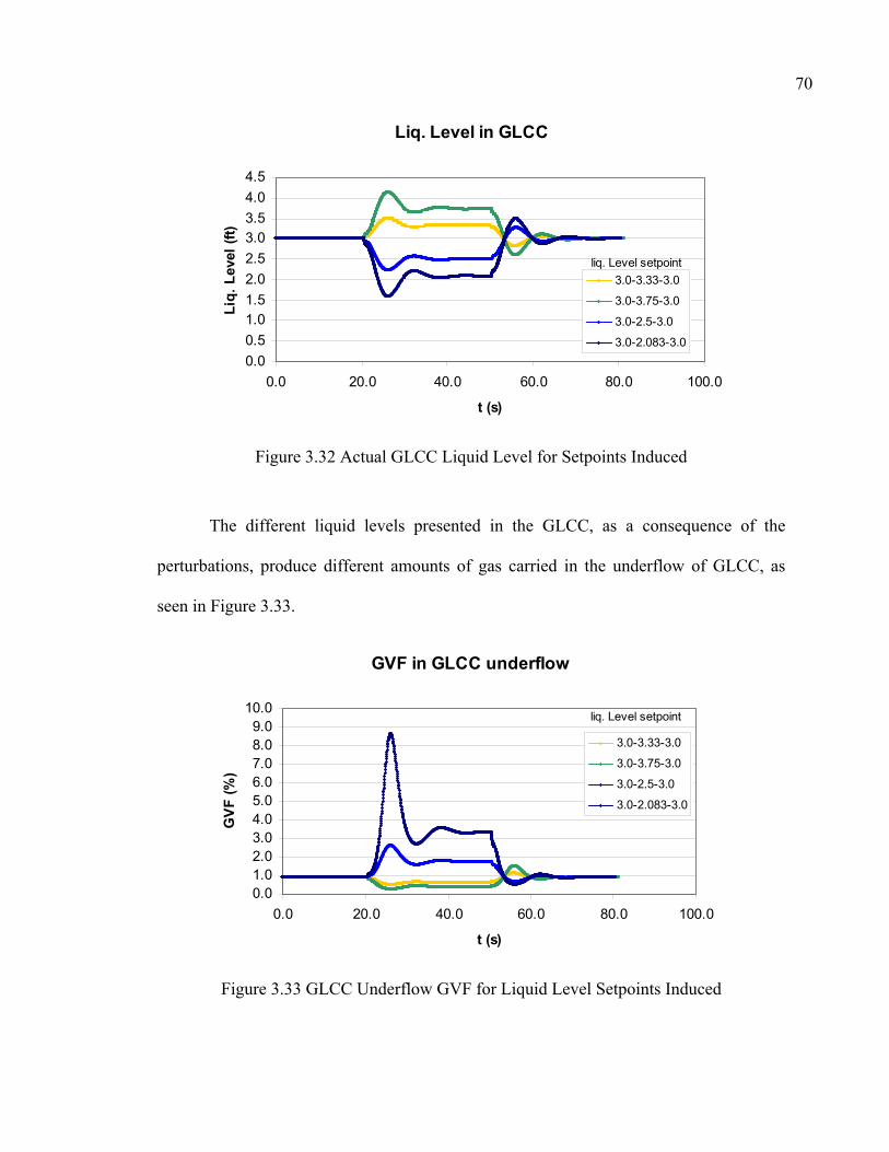
70

Liq. Level in GLCC

0.00.51.01.52.02.53.03.54.04.5

0.0 20.0 40.0 60.0 80.0 100.0

t (s)

Liq.

Lev

el (f

t)

3.0-3.33-3.0

3.0-3.75-3.0

3.0-2.5-3.0

3.0-2.083-3.0

liq. Level setpoint

Figure 3.32 Actual GLCC Liquid Level for Setpoints Induced

The different liquid levels presented in the GLCC, as a consequence of the

perturbations, produce different amounts of gas carried in the underflow of GLCC, as

seen in Figure 3.33.

GVF in GLCC underflow

0.01.02.03.04.05.06.07.08.09.0

10.0

0.0 20.0 40.0 60.0 80.0 100.0

t (s)

GV

F (%

)

3.0-3.33-3.0

3.0-3.75-3.0

3.0-2.5-3.0

3.0-2.083-3.0

liq. Level setpoint

Figure 3.33 GLCC Underflow GVF for Liquid Level Setpoints Induced

71

Split Ratio in LLCC (Qunderflow/Qinlet)

40.0

45.0

50.0

55.0

60.0

65.0

70.0

0.0 20.0 40.0 60.0 80.0

t (s)

SR (%

)

3.0-3.33-3.0

3.0-3.75-3.0

3.0-2.5-3.0

3.0-2.083-3.0

liq. Level setpoint

Figure 3.34 LLCC Split Ratio for Liquid Level Setpoints Induced

Thus, the gas carry-under in the liquid leg of the GLCC is sent to next stage, the

LLCC, affecting its performance. Even if the controlled variable in the LLCC (the

underflow watercut) remains constant, the split ratio oscillates due to the change in the

LLCC efficiency for different gas void fractions, as seen in Figure 3.34.

Even though the split ratio behavior is different for each of the cases studied

above, the response of the watercut control system is very similar. The response is

demonstrated in Figure 3.35. This result is due to the adjustments of the liquid flowrate

coming out of the GLCC for each change in liquid level setpoint.

72

Water Cut in LLCC (underflow)

70.0

75.0

80.0

85.0

90.0

95.0

100.0

20.0 30.0 40.0 50.0

t (s)

wc

(%)

wc (%)

Figure 3.35 Watercut in LLCC (underflow)

ii) GLCC/LLCC system for different LLCC underflow watercut setpoints:

It is also important to verify the sensitivity of the GLCC/LLCC system for

changes in the LLCC underflow watercut setpoint. These changes mainly affect the

operation of the LLCC. The changes induced in the LLCC underflow watercut setpoint

are displayed in Figure 3.36.

73

Water Cut setpoint in LLCC (underflow)

90.091.092.093.094.095.096.097.098.099.0

100.0

15.0 20.0 25.0 30.0 35.0

t (s)

wc

(%) 97-98-97

97-99-97

97-92-97

w c% setpoint

Figure 3.36 LLCC Underflow Watercut Setpoints Induced

The outcome of the LLCC control system is presented in Figure 3.37. All the watercut

setpoints were successfully achieved, while the major overshoot in the response of the

system was for the largest change in the input setpoint.

Water Cut in LLCC (underflow)

90.091.092.093.094.095.096.097.098.099.0

100.0

15.0 20.0 25.0 30.0 35.0

t (s)

wc

(%) 97-98-97

97-99-97

97-92-97

w c% setpoint

Figure 3.37 Actual LLCC Underflow Watercuts for Setpoints Induced

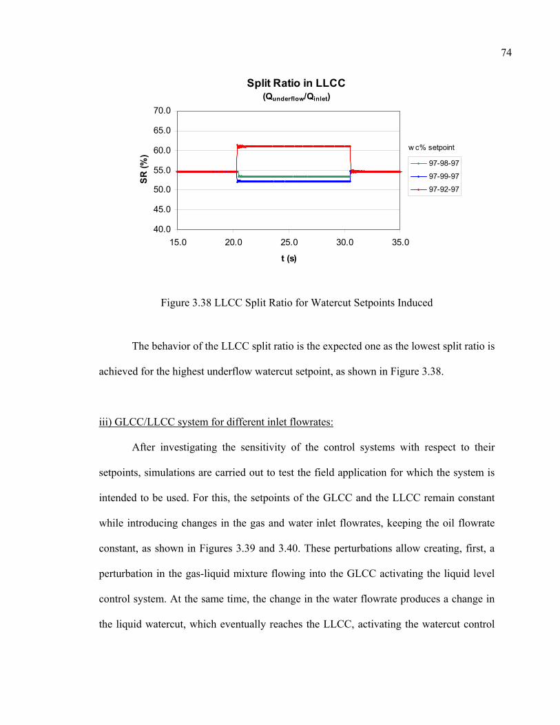
74

Split Ratio in LLCC (Qunderflow/Qinlet)

40.0

45.0

50.0

55.0

60.0

65.0

70.0

15.0 20.0 25.0 30.0 35.0

t (s)

SR (%

)

97-98-97

97-99-97

97-92-97

w c% setpoint

Figure 3.38 LLCC Split Ratio for Watercut Setpoints Induced

The behavior of the LLCC split ratio is the expected one as the lowest split ratio is

achieved for the highest underflow watercut setpoint, as shown in Figure 3.38.

iii) GLCC/LLCC system for different inlet flowrates:

After investigating the sensitivity of the control systems with respect to their

setpoints, simulations are carried out to test the field application for which the system is

intended to be used. For this, the setpoints of the GLCC and the LLCC remain constant

while introducing changes in the gas and water inlet flowrates, keeping the oil flowrate

constant, as shown in Figures 3.39 and 3.40. These perturbations allow creating, first, a

perturbation in the gas-liquid mixture flowing into the GLCC activating the liquid level

control system. At the same time, the change in the water flowrate produces a change in

the liquid watercut, which eventually reaches the LLCC, activating the watercut control

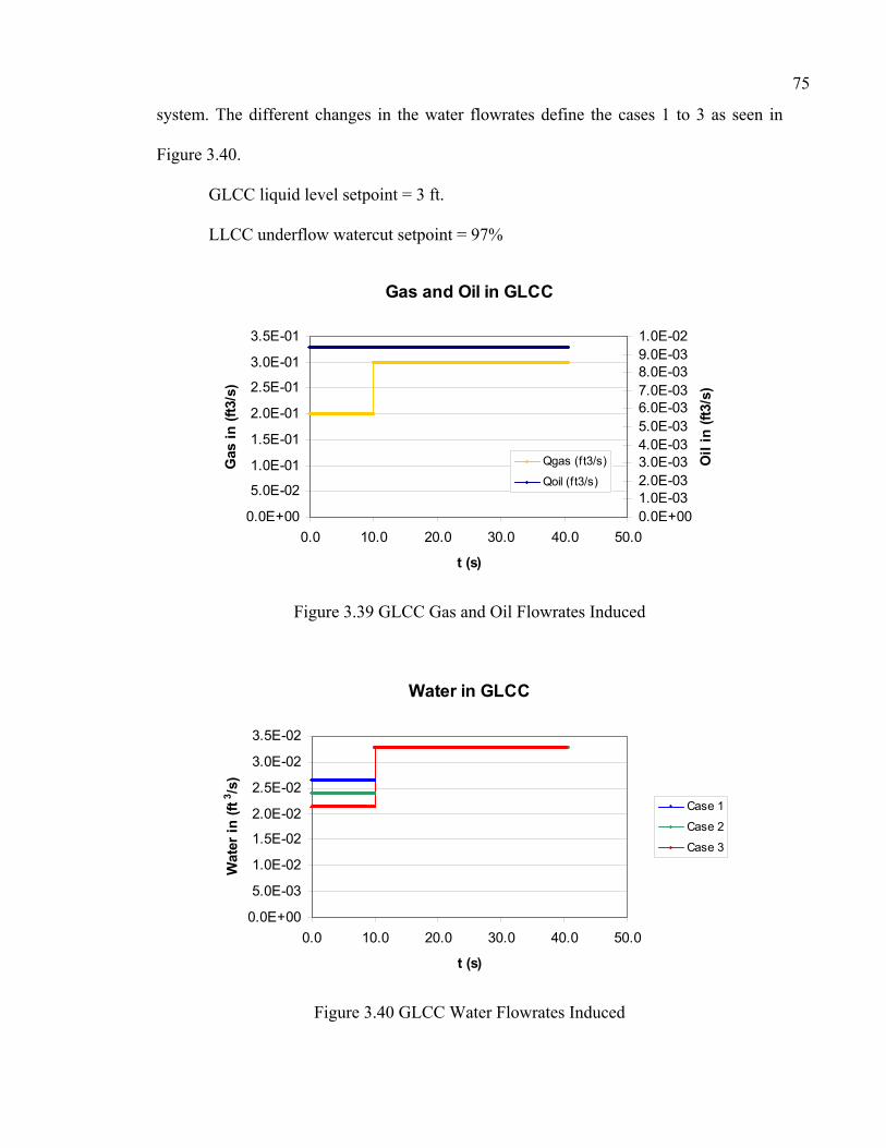
75

system. The different changes in the water flowrates define the cases 1 to 3 as seen in

Figure 3.40.

GLCC liquid level setpoint = 3 ft.

LLCC underflow watercut setpoint = 97%

Gas and Oil in GLCC

0.0E+00

5.0E-02

1.0E-01

1.5E-01

2.0E-01

2.5E-01

3.0E-01

3.5E-01

0.0 10.0 20.0 30.0 40.0 50.0

t (s)

Gas

in (f

t3/s

)

0.0E+001.0E-032.0E-033.0E-034.0E-035.0E-036.0E-037.0E-038.0E-039.0E-031.0E-02

Oil

in (f

t3/s

)

Qgas (ft3/s)

Qoil (ft3/s)

Figure 3.39 GLCC Gas and Oil Flowrates Induced

Water in GLCC

0.0E+00

5.0E-03

1.0E-02

1.5E-02

2.0E-02

2.5E-02

3.0E-02

3.5E-02

0.0 10.0 20.0 30.0 40.0 50.0

t (s)

Wat

er in

(ft3 /s

)

Case 1

Case 2

Case 3

Figure 3.40 GLCC Water Flowrates Induced

76

The dynamic response of the system for these perturbations, while controlling the

GLCC liquid level, is shown in Figure 3.41. It can be seen that the case with the largest

overshoot is Case 1, which presents the smallest change in the liquid flowrate of the three

cases studied. The change in the gas flowrate is the same for all cases. Based on this

observation, since both perturbations are in the same direction (increasing), it is clear that

the liquid flowrate change actually helps to compensate the perturbation introduced by

the change in the gas flowrate.

Liq. Level in GLCC

2.6

2.7

2.8

2.9

3.0

3.1

3.2

0.0 10.0 20.0 30.0 40.0 50.0

t (s)

Liq.

Lev

el (f

t)

Case 1

Case 2

Case 3

Figure 3.41 GLCC Liquid Level for Different Water Flowrates Induced

Since Case 1 reaches the lowest GLCC liquid level, this results in the highest gas

void fraction carried in the liquid leg into the LLCC, as seen in Figure 3.42. The variation

in the gas content in the oil-water mixture leads to changes in the performance of the

LLCC, as can be appreciated in Figure 3.43.

77

GVF in GLCC underflow

0.00.20.40.60.81.01.21.41.61.82.0

0.0 10.0 20.0 30.0 40.0 50.0

t (s)

GVF

(%) Case 1

Case 2

Case 3

Figure 3.42 GLCC Underflow GVF for Different Water Flowrates Induced

Split Ratio in LLCC (Qunderflow/Qinlet)

50.051.052.053.054.055.056.057.058.059.060.0

0.0 10.0 20.0 30.0 40.0

t (s)

SR (%

)

Case 1

Case 2

Case 3

Figure 3.43 LLCC Split Ratio for Different Water Flowrates Induced

78

The controlled variable in the LLCC, the underflow watercut, undertakes the

largest overshoot for Case 3, as this case presents the most important change in the

mixture watercut. This is shown in Figure 3.44.

Water Cut in LLCC (underflow)

75.0

80.0

85.0

90.0

95.0

100.0

10.0 11.0 12.0 13.0 14.0 15.0

t (s)

wc

(%) Case 1

Case 2

Case 3

Figure 3.44 LLCC Underflow Watercut for Different Water Flowrates Induced

3.4 Additional GLCC and LLCC Simulations

Given that the dynamic models for the GLCC and LLCC have already been

developed for absolute values of the control variable, there are other situations that can be

studied without any significant additional effort. These situations include operations such

as start-up, shut down and also the set of separation systems composed of multiple stages.

In this study, examples of such applications are shown next, including: GLCC start-up,

LLCC start-up and a two-stage LLCC separation system, both stages with underflow

watercut control.

79

3.4.1 GLCC Start-Up

Figure 3.45 GLCC Start-up Simulator

The start-up operation of the GLCC can be monitored mainly by the build up of

liquid level starting from zero to the desired final GLCC liquid level setpoint. The major

challenge is how to perform this operation successfully and safely. Different scenarios

can be studied, including increments in the gas-liquid flowrates for a fixed liquid level

setpoint, or increments in the liquid level setpoint for a fixed gas-liquid flowrates. The

last option is studied and presented next. For that, different approaches about how to

change the liquid level setpoint from zero to its final value are proposed, as seen in

Figure 3.46.

80

Liq. Level setpoint in GLCC

0.0

0.5

1.0

1.5

2.0

2.5

3.0

3.5

0.0 20.0 40.0 60.0 80.0 100.0

t (s)

Liq.

Lev

el (f

t)Case 1

Case 2

Case 3

Case 4

Figure 3.46 GLCC Liquid Level Setpoint Inputs

For these moving setpoints, it can be seen that for the sudden change, imposed by

Case 1, the response of the system is a large overshoot (40%). However, while reducing

the slope of the setpoint changes, the overshoot in the liquid level is reduced producing

smooth operations, as shown in Figure 3.47.

Liq. Level in GLCC

-0.50.00.51.01.52.02.53.03.54.04.5

0.0 20.0 40.0 60.0 80.0 100.0

t (s)

Liq.

Lev

el (f

t) Case 1

Case 2

Case 3

Case 4

Figure 3.47 Actual GLCC Liquid Level for Different Setpoint Inputs

81

GVF in GLCC underflow

0.0

5.0

10.0

15.0

20.0

25.0

30.0

0.0 20.0 40.0 60.0 80.0 100.0

t (s)

GVF

(%) Case 1

Case 2

Case 3

Case 4

Figure 3.48 GLCC Underflow GVF for Different Setpoint Inputs

Although Case 4 seems to be the best option for the GLCC start-up, as it is the

case with the lowest overshoot in the liquid level, the results for the GVF in the GLCC

underflow shows a disadvantage of doing this, as seen on Figure 3.48. While increasing

the time where the GLCC is operated with a low liquid level, the amount of gas carried

under through the liquid lines can reach considerable values. In Case 3 it takes 20

seconds to reduce the GVF below 20%, but in Case 4 it takes over 30 seconds to reach

the same point. It is known that even small amount of gas are capable of disturbing the

function of instrumentation connected downstream of the GLCC, hence low liquid level

operations should be avoided.

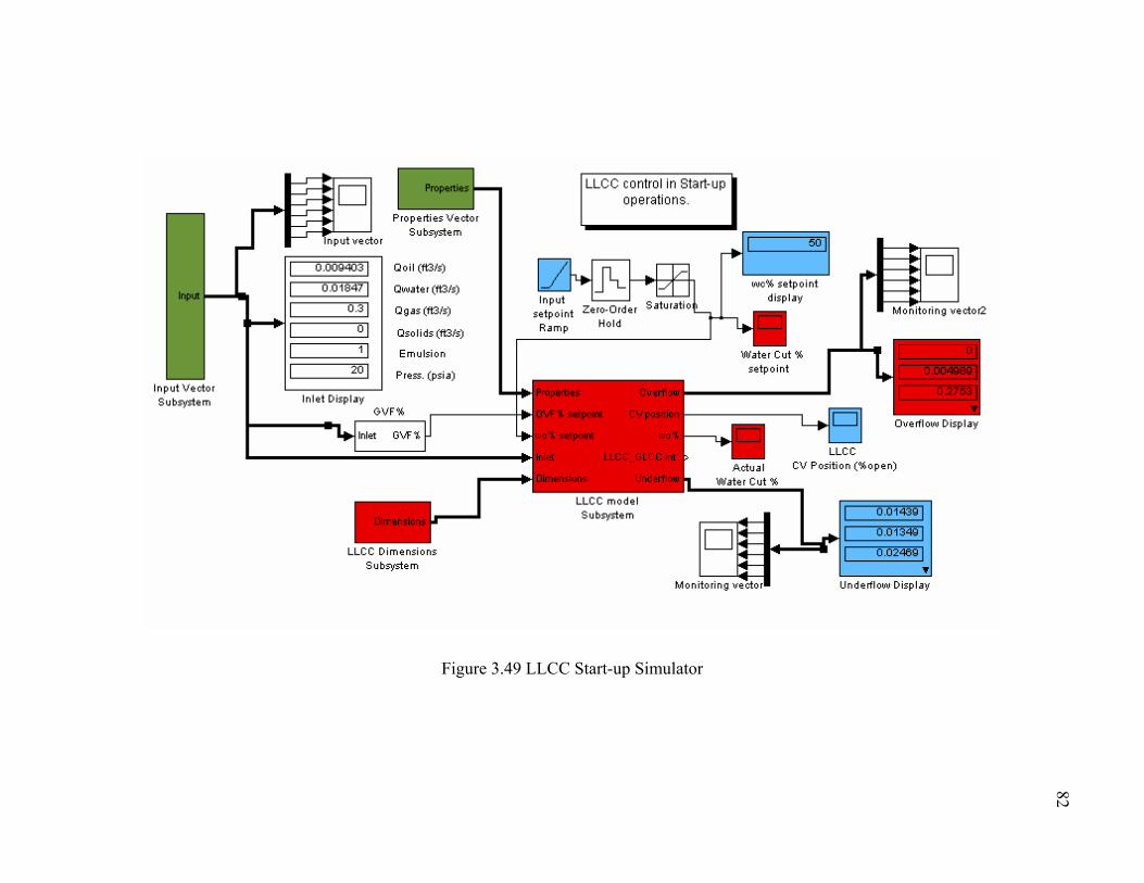
Figure 3.49 LLCC Start-up Simulator

82

83

3.4.2 LLCC Start-Up

The LLCC start-up procedure is very important as well. The LLCC start up

simulator is shown in Figure 3.49. Thus, different actions as shown in Figure 3.50 were

studied. These actions change the LLCC underflow watercut setpoint from the inlet

watercut to the final watercut setpoint.

LLCC underflow watercut setpoint

60.0

65.070.0

75.080.0

85.0

90.095.0

100.0

10.0 15.0 20.0 25.0 30.0 35.0

t (s)

wc

(%) Case 1

Case 2

Case 3

Case 4

Case 5

Figure 3.50 LLCC Underflow Watercut Setpoint Inputs

As can be seen in Figure 3.51, the final watercut setpoint can be reached at

different rates of change of the watercut setpoint. However, the fastest the change in the

setpoint is done, the higher the chances are that the watercut reaches a value of 100%. If

the overshoot were too large, the LLCC would be operating at efficiencies lower than the

optimal split ratio.

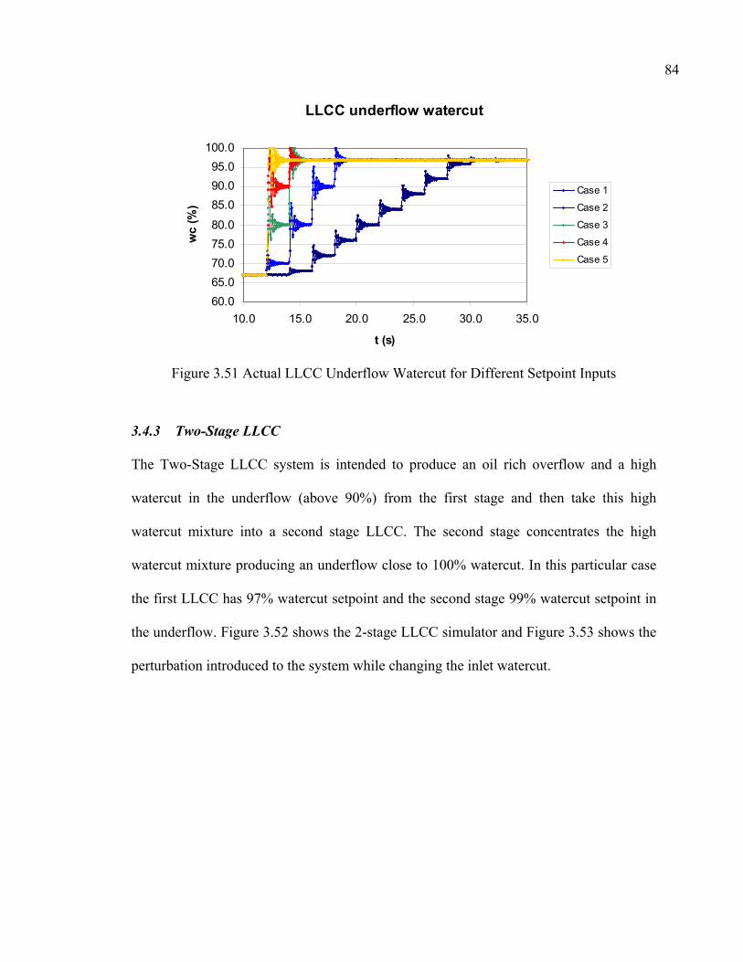
84

LLCC underflow watercut

60.065.070.075.080.0

85.090.095.0

100.0

10.0 15.0 20.0 25.0 30.0 35.0

t (s)

wc

(%)

Case 1

Case 2

Case 3

Case 4

Case 5

Figure 3.51 Actual LLCC Underflow Watercut for Different Setpoint Inputs

3.4.3 Two-Stage LLCC

The Two-Stage LLCC system is intended to produce an oil rich overflow and a high

watercut in the underflow (above 90%) from the first stage and then take this high

watercut mixture into a second stage LLCC. The second stage concentrates the high

watercut mixture producing an underflow close to 100% watercut. In this particular case

the first LLCC has 97% watercut setpoint and the second stage 99% watercut setpoint in

the underflow. Figure 3.52 shows the 2-stage LLCC simulator and Figure 3.53 shows the

perturbation introduced to the system while changing the inlet watercut.

85

Figure 3.52 Two-Stage LLCC Simulator

86

Water and Oil in LLCC

0.0E+00

5.0E-03

1.0E-02

1.5E-02

2.0E-02

2.5E-02

3.0E-02

3.5E-02

0.0 10.0 20.0 30.0 40.0

t (s)

Flow

rate

s in

(ft3 /s

)

Qoil (ft3/s)

Qw at (ft3/s)

Figure 3.53 Input Flowrates into Two-Stage LLCC System

Figures 3.54 and 3.55 present the effect of the control systems in the first and

second LLCC, respectively. While in the first stage LLCC only one main control action is

seen, in the second stage LLCC two control actions are observed. This is due first to the

instantaneous change in the flowrates, as both fluids are incompressible. The second

control action in the second stage LLCC is executed when the mixture with a different

watercut reaches the second stage, the time difference between the first and second action

depends on the length of the pipe connecting both devices.

87

LLCC1 underflow watercut

70.0

75.0

80.0

85.0

90.0

95.0

100.0

0.0 5.0 10.0 15.0 20.0

t (s)

wc

(%)

w c1 (%)

Figure 3.54 First Stage LLCC Underflow Watercut

LLCC2 underflow watercut

70.0

75.0

80.0

85.0

90.0

95.0

100.0

0.0 5.0 10.0 15.0 20.0

t (s)

wc

(%)

w c2 (%)

Figure 3.55 Second Stage LLCC Underflow Watercut

The overflow watercut and the watercut at the inlet of the second stage LLCC

(underflow of first stage LLCC) are shown in Figure 3.56. It is clear that the watercut in

the overflow of the first LLCC is oil-continuous flow for the initial seconds of the

88

simulation. Later on, the fluid is in the water-continuous flow but still is close to the oil-

continuous region. As has been reported by Mathiravedu (2001), the operation of the

LLCC for oil-continuous mixtures (low watercut) is inadequate. This is why for this

particular case the second stage works better operating with the underflow of the first

LLCC (a high watercut mixture). For other operations where the first stage LLCC is

separating high watercut mixtures, the second stage can use the overflow of the first stage

as long as the watercut remains inside the operational envelope of the LLCC.

LLCC 1 & 2 watercuts

30.0

40.0

50.0

60.0

70.0

80.0

90.0

100.0

0.0 10.0 20.0 30.0 40.0 50.0

t (s)

wc

(%) LLCC1 top

LLCC2 inlet

LLCC2 top

Figure 3.56 First and Second Stage LLCC Overflow Watercut and

Second Stage LLCC Inlet Watercut

89

LLCC1 & LLCC2 Split Ratio(Qunderflow/Qinlet)

30.0

35.0

40.0

45.0

50.0

55.0

60.0

0.0 5.0 10.0 15.0 20.0

t (s)

SR (%

)

LLCC1

LLCC2

Figure 3.57 First and Second Stage LLCC Split Ratios

As a final point, the split ratio of the second stage LLCC is lower than the split

ratio of the first stage. This is expected since the change in the inlet/underflow watercut is

much larger in the first stage than in the second. This is shown in Figure 3.57.

90

4. EXPERIMENTAL PROGRAM

This chapter describes the experimental facility and the watercut meters. It also

provides description of detailed experimental investigations that were conducted to

evaluate the performance and dynamics of the GLCC/LLCC system and pertinent

experimental results.

4.1 Experimental Setup

The three-phase oil-water-gas flow loop is housed in the College of Engineering

and Natural Sciences Research building located at the North Campus of The University

of Tulsa. This indoor facility enables experimental investigations to be conducted

throughout the year. The oil-water-gas indoor flow facility is a fully instrumented state-

of-the-art flow loop, capable of testing single separation equipment or combined

separation systems. Figure 4.1 shows a photograph of the oil-water-gas experimental

facility. The experimental setup consists of four major sections: storage and metering

section, GLCC test section, LLCC test section, oil-water-gas separation section and data

acquisition system. A brief description of these components is presented next.

4.1.1 Storage and Metering Section

As shown in Figure 4.2, oil and water are stored in separate tanks, each of 400

gallons capacity. Each tank is connected to two pumps that are equipped with return

lines. The first pump is a model 3656, size 1x2-8, of cast iron construction with a bronze

impeller, John Crane Type 21 mechanical seal, and 10 HP motor rotating at 3600 rpm. It

91 delivers 25 gpm @ 108 psig. The second pump is a model 3656, size 1.5x2-10, of cast

iron construction with a bronze impeller, John Crane Type 21 mechanical seal, and 25 HP

motor rotating at 3600 rpm. It delivers 110 gpm at 150 psig.

Figure 4.1 Experimental Facility

The liquids are pumped from the storage section to the metering section where the

flow rates, densities and temperatures are measured. The metering section comprises of

pressure transducers, temperature transducers, control valves and state-of-the-art

Micromotion® coriolis mass flow meters. The water and oil flow rates are controlled

using Fisher control valves mounted on the water and oil lines, respectively. Both the

water and oil pipelines have check valves mounted on the lines downstream of the control

valves to avoid back flow. The flow rates and densities of both water and oil are

measured using the Micromotion® mass flow meter, before controlling their flow rates.

The oil and water are combined in a mixing-tee to obtain oil-water mixture. A static

92 mixer, parallel to the mixing tee, is added to promote proper mixing of the two liquids. A

compressor with working capacity of 0-1200 scfm at a delivery pressure of 100 psig is

used to supply compressed air for operating the control valves. The compressor also

supplies the air to the flow loop. The airflow rate is controlled by a gas control valve and

metered using a Micromotion mass flow meter. The air and liquid streams are combined

at a mixing tee. Check valves, located downstream of each feeder line, are provided to

prevent back flow.

Figure 4.2 Storage And Metering Section

4.1.2 Test Section

Figure 4.3 shows the GLCC test section. The GLCC body is a 3-inch transparent

PVC pipe with a modular 3-inch inclined tangential inlet. The inlet slot area is 25% of the

cross section area of the inlet pipe. The total height of the GLCC is 7 feet, which is

divided by the inlet into the lower liquid section and the upper gas section. A differential

pressure transducer is mounted on the GLCC to measure the liquid level. A gas control

93 valve is mounted in the gas leg to control the liquid level. An absolute pressure

transducer is used to measure the GLCC gas pressure.

DP

GGaa ss

// OO

ii ll // WW

aa ttee rr

GGaass GGCCVV

OOiill // WWaatteerr ++ GGCCUU

o All units in inches.

o Not to scale.

Top View

2.0

3.0

2.0

2.0

30

40

Figure 4.3 GLCC Test Section

The LLCC, shown schematically in Figure 4.4, is a 6.4 feet, 2-inch ID vertical

pipe, with a 5 feet, 2-inch ID horizontal inlet. The inlet slot area is 25% of the inlet full

bore cross sectional area. The inlet is attached to the vertical section 3.3 feet below the

top. A 1.5-inch ID concentric pipe located at the top is used as the oil outlet, and the

water outlet is a radial, 1.5-inch ID pipe located at the bottom of the vertical section.

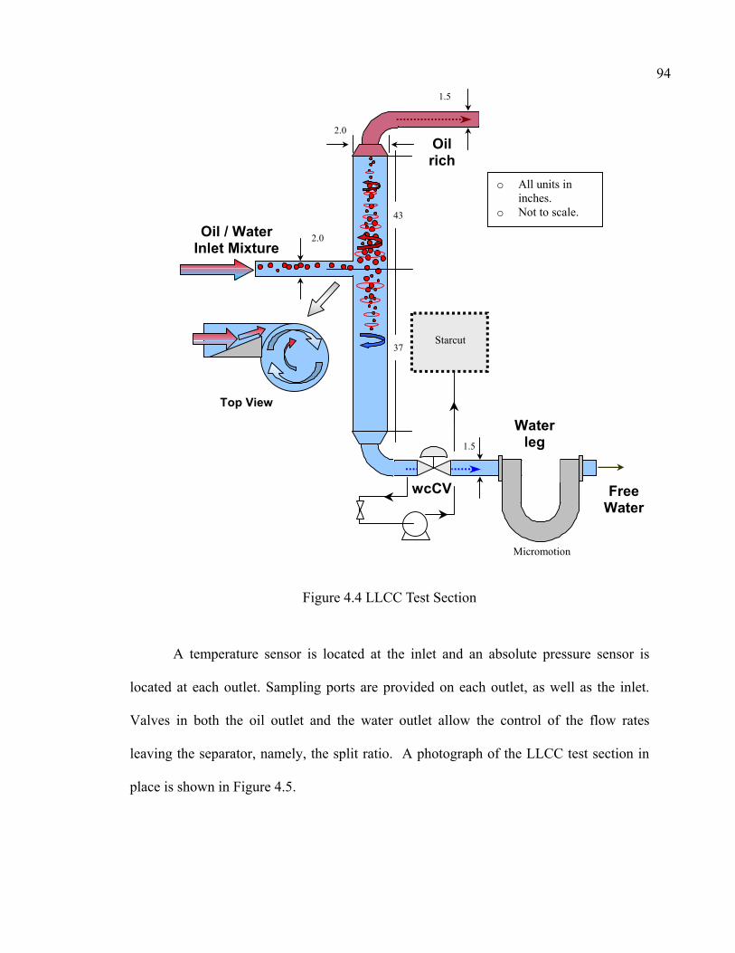
94

Starcut

Micromotion

wcCV

Oil rich

Oil / Water Inlet Mixture

Water leg

Top View

2.0

2.0

1.5

1.5

43

37

o All units in inches.

o Not to scale.

Figure 4.4 LLCC Test Section

A temperature sensor is located at the inlet and an absolute pressure sensor is

located at each outlet. Sampling ports are provided on each outlet, as well as the inlet.

Valves in both the oil outlet and the water outlet allow the control of the flow rates

leaving the separator, namely, the split ratio. A photograph of the LLCC test section in

place is shown in Figure 4.5.

FreeWater

95

Figure 4.5 Photo of LLCC Test Section in Place 4.1.3 Gas-Oil-Water Separation Section

The gas outlet from the GLCC and the two outlet streams from the LLCC test

section finally flow into a three-phase separator. The three-phase separator operates at 5

psig and has a capacity of 528 gallons. It consists of three compartments. In the first

compartment the oil-water mixture is stratified and the oil flows into the second

compartment through floatation. In this compartment, there is a level control system that

activates a control valve discharging the oil into the oil storage tank. The water flows

from the first compartment into the third compartment through a channel below the

second compartment. In this compartment there is a level control system, allowing the

water to flow into the storage tank. The gas is separated in the 3-phase separator as is

discharged through a separate outlet.

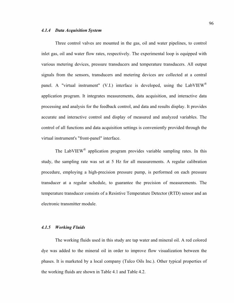
96 4.1.4 Data Acquisition System

Three control valves are mounted in the gas, oil and water pipelines, to control

inlet gas, oil and water flow rates, respectively. The experimental loop is equipped with

various metering devices, pressure transducers and temperature transducers. All output

signals from the sensors, transducers and metering devices are collected at a central

panel. A "virtual instrument" (V.I.) interface is developed, using the LabVIEW®

application program. It integrates measurements, data acquisition, and interactive data

processing and analysis for the feedback control, and data and results display. It provides

accurate and interactive control and display of measured and analyzed variables. The

control of all functions and data acquisition settings is conveniently provided through the

virtual instrument's "front-panel" interface.

The LabVIEW® application program provides variable sampling rates. In this

study, the sampling rate was set at 5 Hz for all measurements. A regular calibration

procedure, employing a high-precision pressure pump, is performed on each pressure

transducer at a regular schedule, to guarantee the precision of measurements. The

temperature transducer consists of a Resistive Temperature Detector (RTD) sensor and an

electronic transmitter module.

4.1.5 Working Fluids

The working fluids used in this study are tap water and mineral oil. A red colored

dye was added to the mineral oil in order to improve flow visualization between the

phases. It is marketed by a local company (Tulco Oils Inc.). Other typical properties of

the working fluids are shown in Table 4.1 and Table 4.2.

97 Table 4.1 Properties of Water Phase

Density, ρ 1.0 ± 0.003 gr/cm3

Viscosity, µ 1.35 ± 0.15 cP

Table 4.2 Properties of Oil Phase

Typical Properties ASTM Test Method Tufflo 6016

Viscosity, SUS

@ 100ºF ( 37.8ºC)

@ 200ºF ( 93.3ºC)

D2161

85

38

Viscosity, cP

@ 100ºF ( 37.8ºC)

@ 200ºF ( 93.3ºC)

13.6

2.8

Viscosity, cSt

@ 104ºF (40ºC)

D 445

15.6

Gravity, ºAPI

Specific Gravity @ 60ºF

Pounds/ Gallons

D 287

D1298

33.7

0.8571

7.14

Viscosity Gravity Constant

Flash Point, ºF (ºC)

Pour Point, ºF (ºC)

D 2501

D 92

D 97

0.81

365 (185)

10 (-12.2)

Aniline Point, ºF (ºC)

Refractive Index @ 20ºC

Molecular Weight

Volatility,22hrs@225ºF,wt%

D 611

D 1218

D 2502

D 972

225 (107.2)

1.469

330

2.0

Distillation, ºF

IBP

95 %

D 2887

535

832

98 The criteria for selecting the oil are as follows:

• Low emulsification

• Fast separation

• Appropriate optical characteristics

• Non-degrading properties

• Non-hazardous

The temperature in the flow loop varied between 70º F and 80º F during the entire

experimental investigation.

4.2 Watercut Measurement Performance in the Presence of Gas

Selecting proper test equipment for production testing is of primary importance if

the best possible results are to be obtained. The accurate measurement of water

concentration in an oil-water mixture is a critical issue in many production operations.

Conventional well testing requires a test trap, test lines and field personnel all of which

are costly. Over the past few years, emphasis has been placed on developing technology

for metering of multiphase wellhead fluids to replace conventional well test systems. The

oil industry has recognized potential for economical savings if dependable watercut

meters could replace conventional test separators, portable test units and well test lines.

The advantages are more significant for operations in offshore and remote onshore areas.

Several watercut meters have been introduced to the oil industry in the last few

years, for measuring oil and water concentrations. Particular concern is the ability of a

meter to provide accurate information for a wide range of flow conditions, such as in the

presence of gas. These meters use different techniques in order to measure the water

99 concentration in an oil-water mixture. In this study, two different watercut meters,

employing different principles, are used. This section provides information about the

meters, configurations, components and principles of operation. The two watercut meters

used in this study are:

a) Coriolis Mass Flow Meter (Micromotion®)

b) Microwave Watercut Meter (Starcut).

4.2.1 Coriolis Mass Flow Meter (Micromotion®)

A Coriolis device such as Micromotion® mass flow-meter, measures the mass

flow rate and mixture density. Thus, it simultaneously serves as both a flow meter and a

watercut analyzer. The major components of the meter are a sensor and a transmitter.

The orientation of a Micromotion mass flow meter is normally recommended by

the manufacturer, and it is based on the particular metering application. For liquid

metering, a tubes down installation is recommended to allow any entrained gas to be

easily moved out of the tube by buoyancy forces, even at low liquid flow rates. Figure 4.6

shows the experimental set-up of the Coriolis meter in the loop.

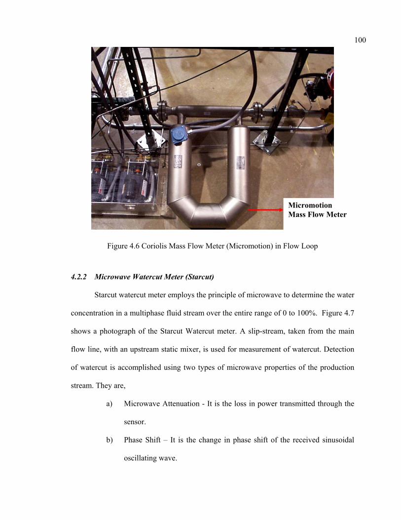
100

Figure 4.6 Coriolis Mass Flow Meter (Micromotion) in Flow Loop

4.2.2 Microwave Watercut Meter (Starcut)

Starcut watercut meter employs the principle of microwave to determine the water

concentration in a multiphase fluid stream over the entire range of 0 to 100%. Figure 4.7

shows a photograph of the Starcut Watercut meter. A slip-stream, taken from the main

flow line, with an upstream static mixer, is used for measurement of watercut. Detection

of watercut is accomplished using two types of microwave properties of the production

stream. They are,

a) Microwave Attenuation - It is the loss in power transmitted through the

sensor.

b) Phase Shift – It is the change in phase shift of the received sinusoidal

oscillating wave.

Micromotion Mass Flow Meter

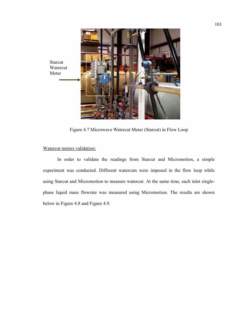
101

Figure 4.7 Microwave Watercut Meter (Starcut) in Flow Loop

Watercut meters validation:

In order to validate the readings from Starcut and Micromotion, a simple

experiment was conducted. Different watercuts were imposed in the flow loop while

using Starcut and Micromotion to measure watercut. At the same time, each inlet single-

phase liquid mass flowrate was measured using Micromotion. The results are shown

below in Figure 4.8 and Figure 4.9.

Starcut Watercut Meter

102

Micromotion vs. StarCut0% gas

50

60

70

80

90

100

50 60 70 80 90 100

wc StarCut (%)

wc

Mic

rom

otio

n (%

)

+ 5%

- 5%

Figure 4.8 Starcut Watercut Measurement Validation (50% to 100%)

Micromotion vs. StarCut0% gas

90

92

94

96

98

100

90 92 94 96 98 100

wc StarCut (%)

wc

Mic

rom

otio

n (%

)

+ 1%

- 1%

Figure 4.9 Starcut Watercut Measurement Validation (90% to 100%)

103 The measurement discrepancy in the 50 to 100% watercut range is between ± 5%

of error. However, for high watercuts (90 to 100%) this error is reduced to the ± 1%

range.

4.2.3 Watercut Measurement Using Micromotion Compensated for Gas Void

Fraction

Mathiravedu (2001) concluded that in general both watercut meters showed very

good agreement for most of the cases studied. But, for low inlet mixture velocities the

microwave meter (Starcut) showed more accurate reading, as compared to the Coriolis

watercut meter (Micromotion).

Contreras (2002) conducted several experiments taking samples from the LLCC

underflow line and comparing with the two watercut meter readings. Experiments were

conducted for a liquid superficial velocity of 1.3 ft/s and different inlet watercuts. It was

observed that better accuracy was obtained with the Starcut meter (1.19%), while with

the Micromotion Meter the error reached up to 7%. Also, the Coriolis Mass Flow Meter

(Micromotion) was not reliable when small amount of gas is entrained into the liquid

phase due to drive gain saturation.

Given that the current study of the GLCC/LLCC system includes the

measurement of the LLCC underflow watercut and that the GLCC produces gas carry-

under, the ability of watercut meters to work properly in the presence of gas becomes

clearly important. In order to study this effect, an experiment was conducted using the

GLCC/LLCC system. While keeping the GLCC liquid level setpoint (35.5 in), the inlet

air mass flowrate (1.2 lb/min), the inlet water mass flowrate (120 lb/min) and the inlet oil

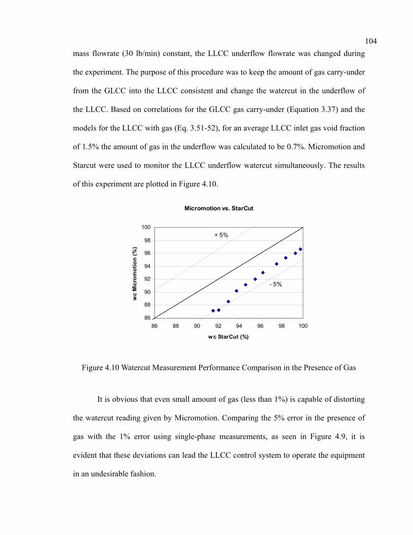
104 mass flowrate (30 lb/min) constant, the LLCC underflow flowrate was changed during

the experiment. The purpose of this procedure was to keep the amount of gas carry-under

from the GLCC into the LLCC consistent and change the watercut in the underflow of

the LLCC. Based on correlations for the GLCC gas carry-under (Equation 3.37) and the

models for the LLCC with gas (Eq. 3.51-52), for an average LLCC inlet gas void fraction

of 1.5% the amount of gas in the underflow was calculated to be 0.7%. Micromotion and

Starcut were used to monitor the LLCC underflow watercut simultaneously. The results

of this experiment are plotted in Figure 4.10.

Micromotion vs. StarCut

86

88

90

92

94

96

98

100

86 88 90 92 94 96 98 100

wc StarCut (%)

wc

Mic

rom

otio

n (%

)

+ 5%

- 5%

Figure 4.10 Watercut Measurement Performance Comparison in the Presence of Gas

It is obvious that even small amount of gas (less than 1%) is capable of distorting

the watercut reading given by Micromotion. Comparing the 5% error in the presence of

gas with the 1% error using single-phase measurements, as seen in Figure 4.9, it is

evident that these deviations can lead the LLCC control system to operate the equipment

in an undesirable fashion.

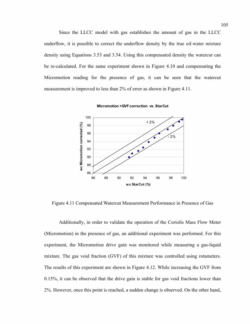
105 Since the LLCC model with gas establishes the amount of gas in the LLCC

underflow, it is possible to correct the underflow density by the true oil-water mixture

density using Equations 3.53 and 3.54. Using this compensated density the watercut can

be re-calculated. For the same experiment shown in Figure 4.10 and compensating the

Micromotion reading for the presence of gas, it can be seen that the watercut

measurement is improved to less than 2% of error as shown in Figure 4.11.

Micromotion +GVF correction vs. StarCut

86

88

90

92

94

96

98

100

86 88 90 92 94 96 98 100

wc StarCut (%)

wc

Mic

rom

otio

n co

rrec

ted

(%) + 2%

- 2%

Figure 4.11 Compensated Watercut Measurement Performance in Presence of Gas

Additionally, in order to validate the operation of the Coriolis Mass Flow Meter

(Micromotion) in the presence of gas, an additional experiment was performed. For this

experiment, the Micromotion drive gain was monitored while measuring a gas-liquid

mixture. The gas void fraction (GVF) of this mixture was controlled using rotameters.

The results of this experiment are shown in Figure 4.12. While increasing the GVF from

0.15%, it can be observed that the drive gain is stable for gas void fractions lower than

2%. However, once this point is reached, a sudden change is observed. On the other hand,

106 if the experiment is carried in the other direction (reducing the GVF), it can be seen that

this sudden change happens at 1.35% GVF in the opposite direction, showing a hysterisis

phenomenon.

Drive Gain (V)

0

2

4

6

8

10

12

0.1 1.0 10.0 100.0GVF (%)

Driv

e G

ain

(V)

Figure 4.12 Micromotion Drive Gain for Different Gas Void Fractions

Based on this behavior, the experimental data using Micromotion to measure the

watercut in the presence of gas are validated since all the experiments were carried for

GVF lower than 1%. Then, for these amounts of gas, the drive gain should remain stable

in the left side region of Figure 4.12.

4.3 Inversion Point Determination

Since the continuous phase is one of the variables in the system mathematical

model, experimental validation of the inversion point for oil-water mixtures is required.

The experiment was conducted using the microwave watercut meter (Starcut). Starcut

provides a variable describing the continuous phase based on built-in algorithms by

analyzing continuously the microwave attenuation and the phase shift. The results of this

107 experiment are presented in Figure 4.13. As it can be seen, the hysterisis effect is

captured even for a narrow range.

Continuous Phase based on StarCut

0

0.5

1

44 45 46 47 48 49 50

wc (%)

Con

tinuo

us P

hase

Water Continuous

Oil Continuous

Figure 4.13 Inversion Point for Oil-Water mixture based on Starcut.

4.4 Transient Data

After validating the watercut meters and studying the system from the modeling

point of view, as presented in Chapter 3, an experimental investigation of the

GLCC/LLCC system and the control systems was conducted. Different experiments were

performed in order to test the system response for different scenarios, such as GLCC

liquid level setpoint as a perturbation, LLCC underflow watercut setpoint as a

perturbation and the change in the inlet flowrates as a perturbation. Additionally, some

important factors in the interaction of the GLCC and the LLCC are emphasized, for

instance, the effect of the gas carry-under from the GLCC underflow on the LLCC

performance.

108 The PID values used during the experimental program for the GLCC controller

and the LLCC controller are given in Table 4.3.

Table 4.3 PID Settings for GLCC and LLCC Controllers during Experiments GLCC Settings LLCC Settings

P 1.5230 Kp 1.5230 P 1.3339 Kp 1.3339 I (s-1) 0.2561 Ti (min) 0.0991 I (s-1) 0.1049 Ti (min) 0.2120 D (s) 1.8093 Td (min) 0.0198 D (s) 3.3934 Td (min) 0.0424

4.4.1 GLCC Liquid Level Setpoint as a Perturbation

For this test a set of different setpoints were induced to the system while

monitoring its behavior. Changes in the GLCC liquid level were made from the inlet

level to setpoints above and below the inlet, as shown in Figure 4.14.

GLCC level setpoint (in)

0.05.0

10.015.020.025.030.035.040.045.050.0

0 50 100 150 200 250t (s)

Liq.

Lev

el s

etpo

int (

in)

35.5-45-35.5

35.5-40-35.5

35.5-30-35.5

35.5-25-35.5

Figure 4.14 GLCC Liquid Level Setpoints Induced

The response of the control system can be appreciated in Figure 4.15. It can be

seen that for each setpoint specified, the control system adjusts the gas control valve until

Liq. Level (in)

109 the actual level matches the desired value. For the particular settings of the experimental

facility, the maximum overshoot was achieved while changing the setpoint from 35.5 to

25 inches, reaching a value of 22%. These experiments were performed while keeping

the LLCC underflow watercut setpoint constant at 97% and the inlet flowrates constant

(120 lb/min of water, 30 lb/min of oil and 0.4 lb/min of air). The values of the actual

watercut can be seen in Figure 4.16, while the split ratio during the operation is displayed

in Figure 4.17.

GLCC level (in)Changes in setpoint

0.0

10.0

20.0

30.0

40.0

50.0

60.0

0.0 50.0 100.0 150.0 200.0 250.0t (s)

Liq.

Lev

el (i

n)

35.5-30-35.5

35.5-25-35.5

35.5-40-35.5

35.5-45-35.5

Figure 4.15 GLCC Liquid Level Response for Setpoints Induced

Liq. Level (in)

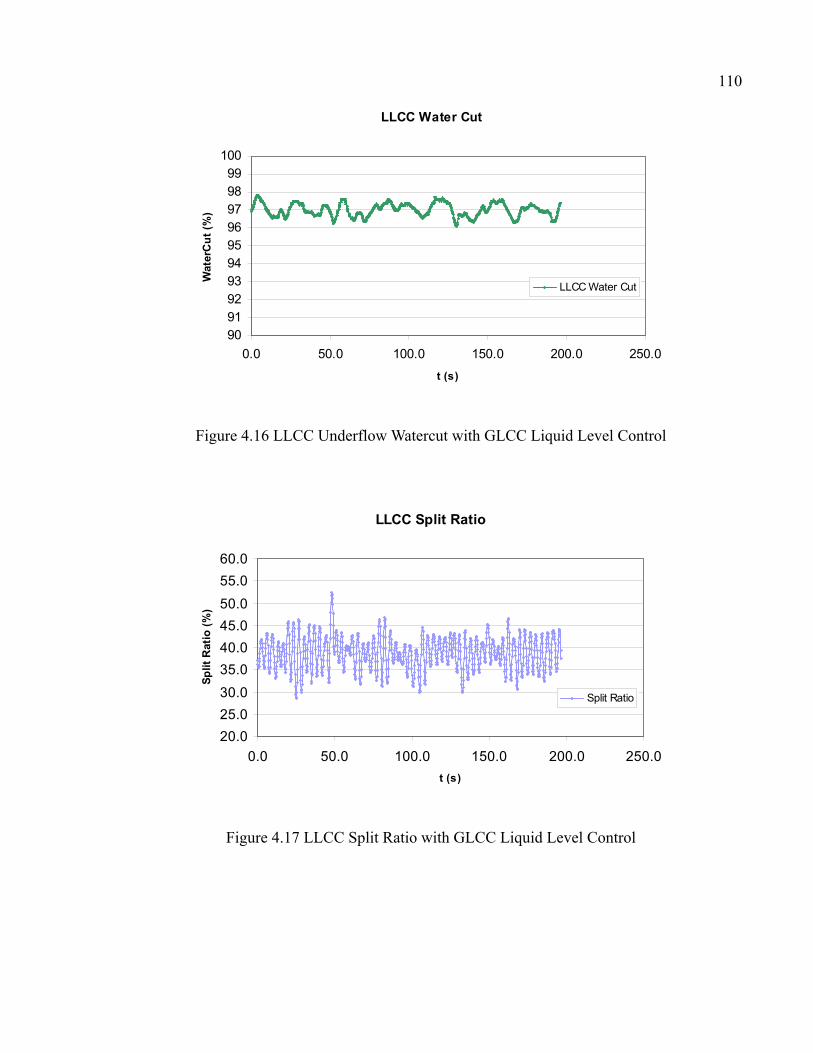
110

LLCC Water Cut

90919293949596979899

100

0.0 50.0 100.0 150.0 200.0 250.0t (s)

Wat

erC

ut (%

)

LLCC Water Cut

Figure 4.16 LLCC Underflow Watercut with GLCC Liquid Level Control

LLCC Split Ratio

20.025.030.035.040.045.050.055.060.0

0.0 50.0 100.0 150.0 200.0 250.0t (s)

Split

Rat

io (%

)

Split Ratio

Figure 4.17 LLCC Split Ratio with GLCC Liquid Level Control

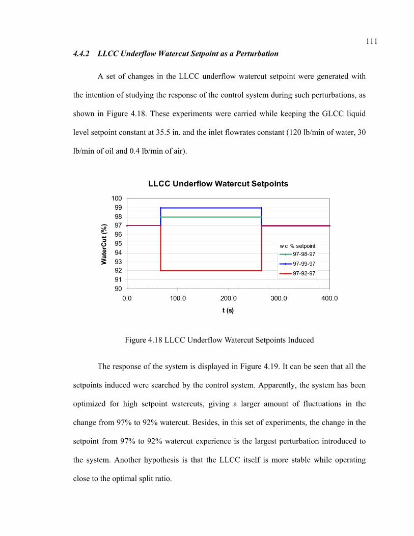
111 4.4.2 LLCC Underflow Watercut Setpoint as a Perturbation

A set of changes in the LLCC underflow watercut setpoint were generated with

the intention of studying the response of the control system during such perturbations, as

shown in Figure 4.18. These experiments were carried while keeping the GLCC liquid

level setpoint constant at 35.5 in. and the inlet flowrates constant (120 lb/min of water, 30

lb/min of oil and 0.4 lb/min of air).

LLCC Underflow Watercut Setpoints

90919293949596979899

100

0.0 100.0 200.0 300.0 400.0

t (s)

Wat

erC

ut (%

)

97-98-97

97-99-97

97-92-97

w c % setpoint

Figure 4.18 LLCC Underflow Watercut Setpoints Induced

The response of the system is displayed in Figure 4.19. It can be seen that all the

setpoints induced were searched by the control system. Apparently, the system has been

optimized for high setpoint watercuts, giving a larger amount of fluctuations in the

change from 97% to 92% watercut. Besides, in this set of experiments, the change in the

setpoint from 97% to 92% watercut experience is the largest perturbation introduced to

the system. Another hypothesis is that the LLCC itself is more stable while operating

close to the optimal split ratio.

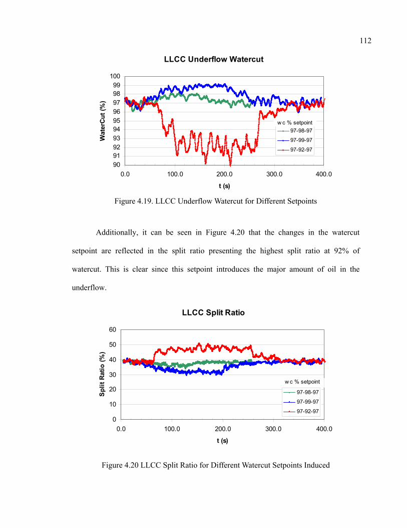
112

LLCC Underflow Watercut

90919293949596979899

100

0.0 100.0 200.0 300.0 400.0

t (s)

Wat

erC

ut (%

)

97-98-97

97-99-97

97-92-97

w c % setpoint

Figure 4.19. LLCC Underflow Watercut for Different Setpoints

Additionally, it can be seen in Figure 4.20 that the changes in the watercut

setpoint are reflected in the split ratio presenting the highest split ratio at 92% of

watercut. This is clear since this setpoint introduces the major amount of oil in the

underflow.

LLCC Split Ratio

0

10

20

30

40

50

60

0.0 100.0 200.0 300.0 400.0

t (s)

Spl

it R

atio

(%)

97-98-97

97-99-97

97-92-97

w c % setpoint

Figure 4.20 LLCC Split Ratio for Different Watercut Setpoints Induced

113 4.4.3 Inlet Flowrates and Watercut as a Perturbation for the GLCC/LLCC System

At this point and after testing the system for different setpoints in the GLCC

liquid level and the LLCC underflow watercut, additional tests of the behavior of the

system for different flow conditions are presented. The setpoints of the GLCC liquid

level and the LLCC underflow watercut are kept constant at 35.5 in and 97%

respectively. The changes in air mass flowrates are common for all tests as shown in

Figure 4.21. The oil mass flowrate is kept constant as shown in Figure 4.22.

Air Mass Flow In

0

0.1

0.2

0.3

0.4

0.5

0 100 200 300 400 500

t (s)

Mas

s flo

w ra

te (l

b/m

in)

Air Mass Flow In

Figure 4.21 Inlet Air Mass Flowrate

The inlet water mass flowrate was changed at different values, as displayed in

Figure 4.23, defining cases 1, 2 and 3. This kind of perturbation was done with a dual

purpose: one, to alter the GLCC steady-state simultaneously with the change in the air

mass flow in, and two, to change the LLCC steady-state since the watercut of the mixture

is modified.

114

Oil Mass Flow In

0

5

10

15

20

25

30

35

0 100 200 300 400 500

t (s)

Mas

s flo

w ra

te (l

b/m

in)

Oil Mass Flow In

Figure 4.22 Inlet Oil Mass Flowrate

Water Mass Flowrate In

0

20

40

60

80

100

120

140

0 100 200 300 400 500

t (s)

Mas

s flo

w r

ate

(lb/m

in)

Case 1

Case 2

Case 3

Figure 4.23 Inlet Water Mass Flow

In Figure 4.24, the oscillations due to the action of the control system in order to

keep the GLCC liquid level around the setpoint can be observed. The overshoot in the

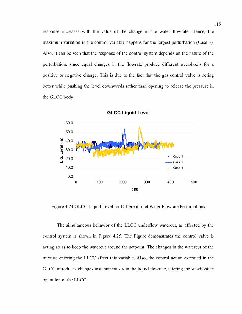
115 response increases with the value of the change in the water flowrate. Hence, the

maximum variation in the control variable happens for the largest perturbation (Case 3).

Also, it can be seen that the response of the control system depends on the nature of the

perturbation, since equal changes in the flowrate produce different overshoots for a

positive or negative change. This is due to the fact that the gas control valve is acting

better while pushing the level downwards rather than opening to release the pressure in

the GLCC body.

GLCC Liquid Level

0.0

10.0

20.0

30.0

40.0

50.0

60.0

0 100 200 300 400 500

t (s)

Liq.

Lev

el (i

n)

Case 1

Case 2

Case 3

Figure 4.24 GLCC Liquid Level for Different Inlet Water Flowrate Perturbations

The simultaneous behavior of the LLCC underflow watercut, as affected by the

control system is shown in Figure 4.25. The Figure demonstrates the control valve is

acting so as to keep the watercut around the setpoint. The changes in the watercut of the

mixture entering the LLCC affect this variable. Also, the control action executed in the

GLCC introduces changes instantaneously in the liquid flowrate, altering the steady-state

operation of the LLCC.

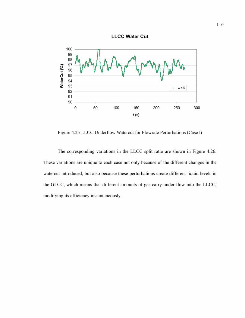
116

LLCC Water Cut

90919293949596979899

100

0 50 100 150 200 250 300

t (s)

Wat

erC

ut (%

)

w c%

Figure 4.25 LLCC Underflow Watercut for Flowrate Perturbations (Case1)

The corresponding variations in the LLCC split ratio are shown in Figure 4.26.

These variations are unique to each case not only because of the different changes in the

watercut introduced, but also because these perturbations create different liquid levels in

the GLCC, which means that different amounts of gas carry-under flow into the LLCC,

modifying its efficiency instantaneously.

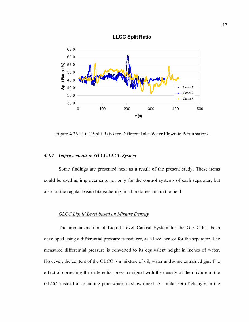
117

LLCC Split Ratio

30.0

35.0

40.0

45.0

50.0

55.0

60.0

65.0

0 100 200 300 400 500

t (s)

Split

Rat

io (%

)

Case 1

Case 2

Case 3

Figure 4.26 LLCC Split Ratio for Different Inlet Water Flowrate Perturbations

4.4.4 Improvements in GLCC/LLCC System

Some findings are presented next as a result of the present study. These items

could be used as improvements not only for the control systems of each separator, but

also for the regular basis data gathering in laboratories and in the field.

GLCC Liquid Level based on Mixture Density

The implementation of Liquid Level Control System for the GLCC has been

developed using a differential pressure transducer, as a level sensor for the separator. The

measured differential pressure is converted to its equivalent height in inches of water.

However, the content of the GLCC is a mixture of oil, water and some entrained gas. The

effect of correcting the differential pressure signal with the density of the mixture in the

GLCC, instead of assuming pure water, is shown next. A similar set of changes in the

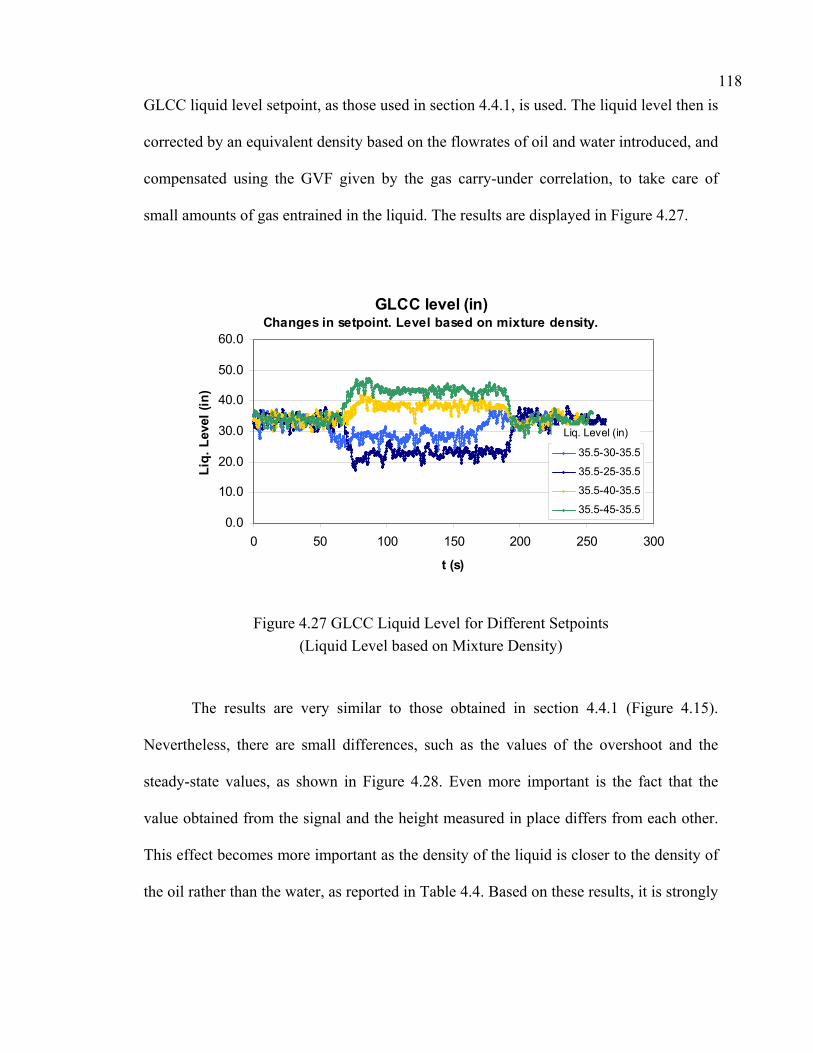
118 GLCC liquid level setpoint, as those used in section 4.4.1, is used. The liquid level then is

corrected by an equivalent density based on the flowrates of oil and water introduced, and

compensated using the GVF given by the gas carry-under correlation, to take care of

small amounts of gas entrained in the liquid. The results are displayed in Figure 4.27.

GLCC level (in)Changes in setpoint. Level based on mixture density.

0.0

10.0

20.0

30.0

40.0

50.0

60.0

0 50 100 150 200 250 300

t (s)

Liq.

Lev

el (i

n)

35.5-30-35.5

35.5-25-35.5

35.5-40-35.5

35.5-45-35.5

Liq. Level (in)

Figure 4.27 GLCC Liquid Level for Different Setpoints (Liquid Level based on Mixture Density)

The results are very similar to those obtained in section 4.4.1 (Figure 4.15).

Nevertheless, there are small differences, such as the values of the overshoot and the

steady-state values, as shown in Figure 4.28. Even more important is the fact that the

value obtained from the signal and the height measured in place differs from each other.

This effect becomes more important as the density of the liquid is closer to the density of

the oil rather than the water, as reported in Table 4.4. Based on these results, it is strongly

119 recommended to include the effect of the true-liquid density in the GLCC liquid level

control for low watercut systems.

GLCC level (in)Changes in setpoint (35.5 in to 45 in)

0.0

10.0

20.0

30.0

40.0

50.0

60.0

0.0 50.0 100.0 150.0 200.0 250.0 300.0

t (s)

Liq.

Lev

el (i

n)

in H2O

mix. Density

OS=5.1%

OS=6.8%

Figure 4.28 GLCC Liquid Level Measurement Comparison with and without Mixture Density Correction

Table 4.4 Offset in Liquid Level Signal with and without Mixture Density Correction

wc% density (g/cc)

Setpoint (in)

Actual level (in)

Offset (in) %error

80.0 1.000 35.5 37.6 2.1 5.58 80.0 0.954 35.5 35.4 -0.1 0.20 20.0 1.000 35.5 44.7 9.2 20.55 20.0 0.872 35.5 36.4 0.9 2.50

120 LLCC Split Ratio for Different LLCC Underflow Watercut Setpoints

Once the concept for a proper watercut measurement performance in the presence

of gas is proven, as shown in section 4.2.3, it was necessary to consider the effect of the

type of watercut measurement for different conditions in the system studied. As a first

case, it is shown how the performance of the LLCC for different watercut setpoints is

evaluated, while a constant liquid level is kept at the GLCC. Also, the flowrates are kept

constant during these runs. Actually, this set of experiments is carried under exactly the

same conditions as those in section 4.4.2 (LLCC Underflow Watercut Setpoint as a

Perturbation). The changes induced to the system are also as those shown in Figure 4.18.

Comparison between the watercut measurement using Micromotion and using

Micromotion with GVF compensation are shown in Figure 4.29, Figure 4.30 and Figure

4.31 for different changes in watercut setpoint.

LLCC WaterCut97%-98%-97% Setpoint

90919293949596979899

100

0 50 100 150 200 250 300

t (s)

Wat

erCu

t (%

)

GVF correction

Micromotion

Figure 4.29 LLCC Underflow Watercut (97%-98%-97% Setpoint)

121

LLCC WaterCut97%-99%-97% Setpoint

90919293949596979899

100

0 50 100 150 200 250 300

t (s)

Wat

erCu

t (%

)

GVF correction

Micromotion

Figure 4.30 LLCC Underflow Watercut (97%-99%-97% Setpoint)

LLCC WaterCut97%-92%-97% Setpoint

90919293949596979899

100

0 50 100 150 200 250 300 350 400

t (s)

Wat

erCu

t (%

)

GVF correction

Micromotion

Figure 4.31 LLCC Underflow Watercut (97%-92%-97% Setpoint)

122 As can be seen, the watercut measurement values obtained correspond to the

setpoints imposed for each case studied. The main difference is the higher noise level

presented in the GVF compensated signal. This noise is due to the fact that the GVF

compensated signal contains the original signal given by Micromotion and is also

affected by the noise from the GLCC liquid level signal since this variable is used to

compute the amount of gas carry-under transported to the LLCC.

Apparently there is no added value adopting the GVF compensated signal since

both sets of experiments report the same watercut with similar dynamics. However, if the

performance of the LLCC for both cases is compared through the Split Ratio, it is clear

that the GVF compensated method results in higher split ratios than when using the

original signal from Micromotion, as seen on Figure 4.32 and Figure 4.33. This

phenomenon is explained by the fact that the original signal from Micromotion does not

take into account the presence of gas in the mixture. Thus, the watercut reported using

Micromotion is actually higher, since the gas present in the mixture is taken as part of the

oil phase. Thus, it is highly recommended to include the effect of the gas in watercut

meters in order to optimize the performance of separators, such as the LLCC.

123

LLCC Split RatioWatercut measured using Micromotion

0

10

20

30

40

50

60

0.0 100.0 200.0 300.0 400.0

t (s)

Split

Rat

io (%

)

97-98-97

97-99-97

97-92-97

w c % setpoint

Figure 4.32 LLCC Split Ratio Obtained using Micromotion to Measure Watercut

LLCC Split Ratio Watercut measured using Micromotion GVF compensated

0

10

20

30

40

50

60

0 100 200 300 400

t (s)

Split

Rat

io (%

)

97-98-97

97-99-97

97-92-97

w c % setpoint

Figure 4.33 LLCC Split Ratio Obtained using GVF Compensated Micromotion to Measure Watercut

124 LLCC Split Ratio for Different GLCC Liquid Level Setpoints

As mentioned in the previous section, it is important to consider the effect of gas

in a watercut meter, since this instrument determines the proper control of a liquid-liquid

separator. With the intention of continuing the study of the GLCC/LLCC system

performance while measuring watercut with or without gas void fraction correction, some

additional experiments were conducted. The set of experiments is similar as those

performed in section 4.4.1 (GLCC Liquid Level Setpoint as a Perturbation) aiming at

comparing both sets of experiments. Similar step changes in the GLCC liquid level

setpoint were induced, as those displayed in Figure 4.14. The responses of the GLCC

liquid level control system for each perturbation are shown in Figure 4.34.

GLCC Liquid Level

0.0

10.0

20.0

30.0

40.0

50.0

60.0

0 100 200 300 400 500

t (s)

Liq.

Lev

el (i

n)

35.5-45-35.5

35.5-40-35.5

35.5-30-35.5

35.5-25-35.5

35.5-20-35.5

Liq. Level (in)

Figure 4.34 GLCC Liquid Level for Different Setpoints

It is critical to note that the performance of the LLCC depends on the GLCC

liquid level setpoint, which corresponds to a different value of gas carry-under. As

125 explained before, the amount of gas injected to the LLCC affects its performance. For a

fixed LLCC underflow watercut setpoint of 97%, the Split Ratio obtained, using

Micromotion as the watercut meter, was below 40% for all the runs, as seen in Figure

4.35.

Figure 4.35 LLCC Split Ratio for Different GLCC Liquid Level Setpoints (Watercut Measured using Micromotion)

However, for those runs for which the GVF compensated Micromotion was used

as a watercut meter, the Split Ratio achieved was increased progressively as the GLCC

liquid level setpoint was decreased, as shown in Figure 4.36. This occurs as a result of the

increment in the gas carry-under that corresponds to lowering the GLCC liquid level. As

reported by Contreras (2002), the gas introduced to the LLCC may increase its efficiency,

yet there is a limit where beyond which this effect is completely reversed. In Figure 4.36,

the experiment for which the GLCC liquid level setpoint was changed from 35.5 to 20

inches demonstrates the highest Split Ratio as compared to other runs. However,

126 observations indicated that for the amount of gas into the LLCC in this run, the LLCC

collapsed since most of the gas diverted into the overflow of the LLCC, creating a slug

flow pattern in the LLCC body.

For the 35.5 to 25 inches liquid level setpoint run, the Split Ratio reaches values

higher than 55%. This high performance of the LLCC can be attributed to the fact that the

gas carry-under in the GLCC was overpredicted. Hence, the gas presence is over

compensated in the reading given by Micromotion.

For the other cases studied (liquid level closer to the GLCC inlet), the gas carry-

under prediction is within a range for which the gas void fraction correction is valid for

the GLCC/LLCC system. As can be seen in Figure 4.36 (Micromotion GVF

compensated) the Split Ratios vary between 42% and 51%, while in Figure 4.35

(Micromotion not compensated) the Split Ratio values obtained are below 40%.

LLCC Split Ratio for different Liq. Level setpointsWaterCut measured using Micromotion GVF compensated

30.0

35.0

40.0

45.0

50.0

55.0

60.0

65.0

70.0

0 100 200 300 400 500

t (s)

Spl

it Ra

tio (%

)

35.5-45-35.535.5-40-35.535.5-30-35.535.5-25-35.535.5-20-35.5

Liq. Level (in)

Figure 4.36 LLCC Split Ratio for Different GLCC Liquid Level Setpoints (Watercut Measured using Micromotion GVF Compensated)

127

5. RESULTS AND DISCUSSION

This chapter presents a discussion on the GLCC/LLCC system mathematical

model developed in this study. Also, discussion of the experimental results, including an

uncertainty analysis, is presented. Finally the direction future investigations might pursue

is presented.

5.1 Mathematical Modeling Discussion

The GLCC/LLCC dynamic simulator developed in Matlab/Simulink® was

successfully tested for different scenarios, including moving setpoints and changes in

input flowrates. The main contribution of this simulator is not only to simulate the

integrated control system for the GLCC and LLCC working simultaneously, but also to

incorporate other phenomena occurring in the system. Models such as gas carry-under,

liquid carry-over, pressure drops, dead time, gas effect on LLCC peformance and others

are included to provide a more realistic performance prediction of the real system.

However, the integrated control system is still based on the linearizations made by Wang

(2000) and Mathiravedu (2001), extending these differential models for an absolute value

model. The next stage in this process is to compare the advantages that a truly absolute

model, based on the original differential equations for the system, would provide instead

of using a differential model. Nevertheless, it has been proven that the proposed approach

is capable of providing more insight, as the simulator is sensitive to the setpoints, and

also since simulations for start-up operations and two-stage LLCC are now available.

128 5.2 Experimental Program Discussion

Before testing the GLCC/LLCC system dynamics in the experimental program, it

was revealed how important it was to validate the proper performance of watercut meters

in the presence of gas. This was demonstrated to be critical in order to improve the

quality of the system investigation. As shown in Chapter 4, it is important to consider the

presence of gas, since this factor improved the readings obtained by Micromotion, while

comparing the results with a watercut meter, such as the Starcut, which is not sensitive to

gas. The inclusion of an uncertainty analysis in this comparison is significant in order to

validate the experimental investigation. In addition, it was essential to validate the values

obtained for the other control variable, the GLCC liquid level. As shown in Chapter 4, the

method used to convert the GLCC differential pressure to liquid height is crucial while

comparing it with the actual level.

5.2.1 Uncertainty Analysis for Watercut Meters

The uncertainty analysis for the watercut meters was based on the data collected

by Contreras (2002), who compared the watercut measurements from Micromotion with

the values obtained using Starcut, while simultaneously taking representative samples of

the mixture to verify the real watercut. The discrepancies between the actual watercuts

and the values reported by the watercut meters were assumed to be equivalent to the

systematic errors given by each instrument. This criterion was established in order to take

into account not only the uncertainty claimed by the manufacturer, but also the real

uncertainty of the instrument installed in place.

129 The uncertainty model used was the simplified U95, as described by Dieck (1997),

namely,

( )2

1

2,

2

95,95,95

+

⋅±= RX

R StBtU

νν (5.1)

where: BR: normally distributed systematic uncertainty at 95% confidence

RXS ,: standard deviation of one result. It is the random uncertainty.

tν,95 : student’s t95 for a given number of degrees of freedom

An example of the results obtained using the uncertainty model for the watercut

meters is shown in Table 5.1. For an input mixture of 95% watercut, the U95 for

Micromotion is 2.978 wc% and the U95 for Starcut is 1.663 wc%.

Table 5.1 Uncertainty Analysis for Watercut Meters

Average WC% t95 BR SX,R U95 Rel. Uncert. (%)Micromotion 95.80 2 2.91 0.5238 2.978 3.11

Starcut 94.91 2.571 0.69 0.5945 1.663 1.75

The validation data for the watercut meters, including the error given by the

uncertainty analysis procedure, are plotted in Figure 5.1. The error bars in this figure are

within the ±5% discrepancy range, mainly for watercuts higher than 65%. A closer look

on the validation data, including the error bars, is seen in Figure 5.2, where the range

from 90 to 100% watercut is plotted. The values obtained with Micromotion differ from

the values obtained with Starcut in the ±1% range. However, the uncertainty bars are

larger than this range.

130

Micromotion vs. StarCut0% gas

50

60

70

80

90

100

50 60 70 80 90 100

wc StarCut (%)

wc

Mic

rom

otio

n (%

)

+ 5%

- 5%

Figure 5.1 Starcut Watercut Meter Validation using Single-Phase Measurements with Micromotion (0% Gas, 50%-100% Watercut Range)

Micromotion vs. StarCut0% gas

90

92

94

96

98

100

90 92 94 96 98 100

wc StarCut (%)

wc

Mic

rom

otio

n (%

)

+ 1%

- 1%

Figure 5.2 Starcut Watercut Meter Validation using Single-Phase Measurements with Micromotion (0% Gas, 90%-100% Watercut Range)

131 Including the uncertainty bars in the comparison for the watercut meters

performance in the presence of gas between Micromotion and Starcut, it is important to

notice that the offset in the watercut given by Micromotion is larger than the uncertainty

of the instrument, as shown in Figure 5.3. This is relevant in order to prove the significant

distortion in the readings obtained by Micromotion in the presence of gas.

Micromotion vs. StarCut

86

88

90

92

94

96

98

100

86 88 90 92 94 96 98 100

wc StarCut (%)

wc

Mic

rom

otio

n (%

)

+ 5%

- 5%

Figure 5.3 Watercut Measurement Performance Comparison in the Presence of Gas

On the other hand, when the comparison between the Micromotion reading

compensated for gas and the values obtained with Starcut, including the uncertainty bars,

as seen on Figure 5.4, are plotted, not only a significant improvement is observed, since

the data is between the ±2% discrepancy range, but also the uncertainty bars are

overlapping the ±2% discrepancy range.

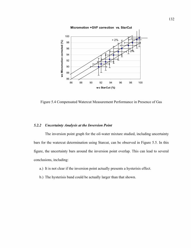
132

Micromotion +GVF correction vs. StarCut

86

88

90

92

94

96

98

100

86 88 90 92 94 96 98 100

wc StarCut (%)

wc

Mic

rom

otio

n co

rrec

ted

(%) + 2%

- 2%

Figure 5.4 Compensated Watercut Measurement Performance in Presence of Gas

5.2.2 Uncertainty Analysis at the Inversion Point

The inversion point graph for the oil-water mixture studied, including uncertainty

bars for the watercut determination using Starcut, can be observed in Figure 5.5. In this

figure, the uncertainty bars around the inversion point overlap. This can lead to several

conclusions, including:

a.) It is not clear if the inversion point actually presents a hysterisis effect.

b.) The hysterisis band could be actually larger than that shown.

133

Continuous Phase based on StarCut

0

0.5

1

44 45 46 47 48 49 50

wc (%)

Con

tinuo

us P

hase

Water Continuous

Oil Continuous

Figure 5.5 Inversion Point for Oil-Water Mixture based on Starcut

5.2.3 Uncertainty Analysis for GLCC Liquid Level Determination

Additionally, the uncertainty model described by Dieck (1997) has been applied

to the GLCC liquid level determination. As shown in Table 5.2, the systematic error

changes, based on which method is used to convert the measured differential pressure

into equivalent liquid height. The criterion to determine the systematic error (BR) is

similar to that applied for the watercut measurement uncertainty. As explained in Chapter

4, there is a difference between the value obtained for the liquid height assuming water

density or mixture density, and the actual value measured in place. It is assumed that this

difference includes not only the uncertainty of the instrument, but also the additional

uncertainties related to its installation in place. Subsequently, even the results for the

uncertainty in the GLCC liquid level show a difference in the systematic errors,

depending on the method used to compute the equivalent liquid height, the values for U95

134 due to the standard deviation contribution, result in similar values for the ultimate U95

(2.948 inches while assuming pure water and 2.829 inches using a mixture density).

Table 5.2 Uncertainty Analysis for GLCC Liquid Level Determination

Actual level (in) t95 BR SX,R U95

Rel. Uncert. (%)

in H2O 37.6 2 2.10 1.0352 2.948 7.84 mix. Density 35.4 2 0.07 1.4138 2.829 7.99

GLCC level Changes in setpoint (35.5 in to 45 in)

0.0

10.0

20.0

30.0

40.0

50.0

60.0

0.0 50.0 100.0 150.0 200.0 250.0 300.0

t (s)

Liq.

Lev

el (i

n)

in H2O

mix. Density

OS=5.1%

OS=6.8%

Figure 5.6 GLCC Liquid Level Comparison With and Without Mixture Density Correction

The differences in the GLCC liquid level when assuming pure water or when

using a mixture density criterion can be observed in Figure 5.6. The respective

uncertainty bars are displayed as well. The U95 values obtained for both criterions are

similar to each other and at the same time, these values are equivalent, as compared to

their respective overshoots.

135 5.2.4 Transient Data Discussion

The measurements based on the GLCC liquid level and the LLCC underflow

watercut can be analyzed after validating these two most important variables for the

GLCC/LLCC system, considering that both of them are the variables to be controlled in

the investigation.

The experiments performed using the GLCC/LLCC system include the response

of the GLCC liquid level control and LLCC watercut control system for different

conditions, as described in Chapter 4. The values reported for the GLCC liquid level in

each run present larger changes than the values found for the uncertainty of this

measurement for most of the experiments. This means that the results obtained for the

GLCC liquid level are conclusive, even if the offset between the real liquid level and the

value measured is not considered. This offset is neglected because all the experiments

were performed using high watercut mixtures, and as discussed previously, for these

cases the offset is not as large as it would be for a low watercut mixture.

On the other hand, the values acquired for the LLCC underflow watercut for some

particular cases such as changes in the watercut setpoint from 97% to 98% (Section

4.4.2), the uncertainty of the measurement is actually larger than the change imposed on

the setpoint of the equipment. Based on this, it can be implied that for such small changes

in the watercut, the action of the control system is affected by the uncertainty of the

instruments. Thus, in order to fine-tune the operation of the separator, improvements in

the watercut metering accuracy would be required.

136

6. CONCLUSIONS AND RECOMMENDATIONS

6.1. Conclusions

The study of the GLCC/LLCC system is not a trivial problem. Even though

separate investigations of each of the existing parts of the system have already been

executed, once integrated in a system, the complexity of the real interactions between the

separators and their control systems might lead to operational problems, such as

instabilities and dramatic reduction in separation efficiency. On the other hand, a proper

management of the resources of the GLCC/LLCC system can also lead to improvement

of the separation efficiency of each stage separately, achieving enhancements in the

performance of the system, not possible before combining them.

Based on the detailed theoretical and experimental investigations of this study, the

following conclusions can be drawn:

1. The complexity of the GLCC©/LLCC© system can be analyzed combining their

linear models for the control systems and auxiliary models, aimed at the study of its

actual performance.

• The developed GLCC©/LLCC© system simulator has been successfully tested for

different perturbations. The set of perturbations included changes in the GLCC

liquid level setpoint, changes in the LLCC underflow watercut setpoint and

changes in the inlet gas and liquid flowrates and inlet mixture watercut,

simultaneously.

• The fact that the control models are based on the physics of the separation

systems, while the auxiliary models help to understand the interaction of the

137

control systems with the surrounding components, provides a more realistic

approach in the simulator developed.

• Even though the control models were developed using a differential approach,

the methodology of the simulator is to express the results in terms of absolute

values that are easier to understand.

• Extended capability has been demonstrated for additional field operations.

Different applications including start-up operations and multiple stage separators

can be studied based on the approach proposed in this study.

2. Improvements in the instrumentation of the GLCC©/LLCC© system can improve the

efficiency of the system.

• Proper GLCC liquid level measurement is crucial in order to avoid an offset

between the value of the control variable being monitored and the actual value in

place. The difference between the real liquid height and the value obtained using

differential pressure transducers can be minimized by correcting the liquid height

for the density of the liquid mixture inside the GLCC body. The correction for

the mixture density becomes more important as the watercut of the liquid mixture

decreases.

• In a separation system such as the GLCC/LLCC system, proper watercut meter

selection can make a significant difference in the optimal performance achieved

by the control systems. Since the LLCC is connected to the GLCC, the use of

watercut meters, which are not sensitive to gas, is crucial in order to accomplish

the optimal split ratio in the LLCC and even avoid instabilities in the system.

138

3. The LLCC© performance can be optimized by manipulating the GLCC© operation.

Given that the operation of the GLCC liquid level control produces substantial

changes in the amount of gas carry-under, and as the LLCC efficiency is affected by

the gas fraction in the mixture, any change in the GLCC liquid level may improve or

deteriorate the LLCC operation. If the GLCC liquid level setpoint is lowered below

the inlet level, the LLCC split ratio increases as the gas carry-under contributes to

improve the liquid-liquid separation efficiency. However, there is a limit (7%)

beyond which the amount of gas carry-under is so large that the effect is reversed and

the LLCC performance is then compromised.

6.2. Recommendations

The following recommendations are made for further studies to expand the scope

of this investigation:

1. Improvements in the control models can be performed by solving fundamental

differential equations, which are non-linear. As explained before, the previous

investigations accomplished for the control systems in the GLCC and the LLCC are

based on linearizations of the basic equations for each system. A more detailed

evaluation of the dynamics involved is necessary so as to consider factors such as

initial conditions and the dampening that the system could provide for different

perturbations under particular conditions.

2. GLCC© liquid level measurement improvements taking into account the liquid

mixture density are strongly recommended mainly for low watercut applications. It is

important to avoid an offset in the liquid level signal since this could mean that the

139

real value is actually larger or smaller than the desired value leading to detriments in

the GLCC performance.

3. The use of watercut meters, which are not sensitive to gas, for the LLCC© underflow

watercut control is crucial, in particular if the inlet liquid mixture is from the GLCC©

liquid leg. As it was demonstrated, the performance of the LLCC can be improved by

proper selection of the watercut meter.

140

NOMENCLATURE

Symbols

A = Constant for linear control valve characteristics

C = Overall flow coefficient

1C = Constant for gas control valve: v

g

CC

gC = Gas control valve flow coefficient

oC = Control valve response time, t, seconds

vC = Liquid control valve flow coefficient

d = GLCC diameter, L, ft

1D = Constant for GLCC geometry

2D = Constant for liquid flow rate calculation

3D = Constant for gas mass balance

4D = Constant for gas flow rate calculation

5D = Constant for effect of pressure on liquid flow rate

6D = Constant for effect of liquid level on pressure

7D = Constant for effect of pressure on gas flow rate

e = Error signal

E = Controller output

f = Friction factor

Fgl = empirical factor

141

g = Acceleration due to gravity

GVF = Gas Void Fraction (%)

cg = Factor of proportionality defined by Newton's second law

( )sG = Feed forward loop transfer function

H = Liquid level, L, ft

( )sH = Feed back loop transfer function

j = Volumetric Flux

k = Controller gain

K = Gain

L = Length of pipe segments

M = Molecular weight

n = Mole number

p = Pneumatic pressure, m/Lt2, psi

P = GLCC pressure, m/Lt2, psi

( )sPD = PD compensator transfer function

( )sPI = PI compensator transfer function

( )sPID = PID compensator transfer function

Q = Volumetric flow rate, L3/t, /sft3

R = Universal gas constant, 10.7317 (lbf/in.2)-ft3/lbmol-R

s = Laplace variable

S.R = Split Ratio (%)

142

t = Time, t, seconds

T = Temperature, T, o R

u = Controller output

U = Controlled variable

V = Volume, L3, ft 3

sgV = Superficial gas velocity, L/t, ft/s

slV = Superficial liquid velocity, L/t, ft/s

V& = Net volume rate, L3/t, ft 3 /s

We = Weber Number

W.C. = Water Cut (%)

x = Control valve position, %

z = Compensator zero

Z = Compressibility factor

Greek Letters

α = gas void fraction

γ = Specific gravity

κ = Fitting flow coefficient

ρ = Density, m/L3, lbm/ft3

τo = Time constant, t, seconds

∆ = Incremental deviation

π = 3.141592…

143

µ = Viscosity

Superscripts

' = Denotes parameters in the gas control loop

mod = Modified variable

Subscripts

c = Controller

Deg = Degree

d = Derivative

G = Gas

GCV = Gas control valve

GLCC = Gas-liquid cylindrical cyclone

i = Integral

in = Into GLCC

L = Liquid

LCV = Liquid control valve

lim = Limit

LLCC = Liquid-liquid cylindrical cyclone

max = Maximum

min = Minimum

m = Number of fittings

144

n = Number of pipe segments

o = oil phase

out = Out of GLCC

p = Proportional

s = System

sl = Superficial-liquid

sg = Superficial-gas

s , set = Set point

test = Test

T = Transmitter

v = Valve

w = water phase

145

REFERENCES

1. Afanador E.: “Oil-Water Separation in Liquid-Liquid Cylindrical Cyclone

Separators,” M.S. Thesis, The University of Tulsa, 1999.

2. Agar, J.: “Method and apparatus for net oil measurement,” U.S Patent 4774680,

September 27, 1988.

3. Al-Mubarak, A.M.: “A new method in calculating Watercut and Oil and Water

volumes using Coriolis Meter”, SPE 38786, presented at SPE Annual Technical

Conference, San Antonio, October 5-8, 1997.

4. Arpandi I.A., Joshi A.R., Shoham, O., Shirazi, S. and Kouba, G.E.: “Hydrodynamics

of Two-Phase Flow in Gas-Liquid Cylindrical Cyclone Separators,” SPE 30683

presented at SPE 70th Annual Meeting, Dallas, October 22-26, 1995, SPE Journal,

December 1996, pp. 427-436.

5. Bandyopadhyay, P.R., Pacifico, G.C. and Gad-el-Hak, M.: “Gas Core Configurations

in a Cyclone-Type Gas-Liquid Separator,” Naval Undersea Warfare Center Division,

Division Newport, Rhode Island, Technical report No. 10308, January 1994.

6. Bednarski, S. and Listewnik, J.: “Hydrocyclones for Simultaneous Removal of Oil

and Solid Particles from Ships' Oily Waters,” Filtration and Separation, March/April

1988, pp. 92-97.

7. Cobb: “Ultrasonic Fluid Composition Meter,” U.S. Patent 5473934, December 12,

1995.

146

8. Contreras, W.: “The effect of inlet gas void fraction on the performance of liquid-

liquid cylindrical cyclone (LLCC©) separator,” M.S. Thesis, The University of Tulsa,

2002.

9. Cowie, D.: “Vertical Caisson Slugcatcher Performance,” presented at the Institution

of Chemical Engineers Conference “Subsea Separation and Transport III,” London,

May 23-24, 1991, Trans IChemE., Vol. 70, part A, January 1992, pp. 25-31.

10. Davies, E.E.: “Compact Separators for Offshore Production,” Proceedings of the 2nd,

New Technology for the Exploration & Exploitation of Oil and Gas Resources

Symposium. Luxembourg, 5 Dec. 1984. London, BP Research Center, 1985, Vol. 1,

pp. 621-629.

11. Davies, E.E. and Watson, P.: “Miniaturized Separators for Offshore Platforms,”

Proceedings of the 1st New Technology for Exploration & Exploitation of Oil and

Gas Reserves Symposium, Luxembourg, April 1979, pp. 75-85.

12. Dieck, R.: “Measurement Uncertainty: Methods and Applications,” ISA, 1997, pp 45.

13. Durrett, M.G., Marrelli, J.D., Hatton, G.J. and Helms, D.A.: “Texaco watercut

Monitor- Microwave Based Technology,” Proceedings Indonesian Petroleum

Association, Eighteenth Annual Convention, Indonesia, October 1989.

14. Fekete, L.A.: “Vortex Tube Separator May Solve Weight/Space Limitations,” World

Oil, July 1986, pp. 40-44.

15. Fisher Controls Product Catalog, USA, 1998.

147

16. Gaisford, S.G., Watjen, J.P. and Bjornsen, B.G.: “Composition Monitor and

Monitoring Process using Impedance Measurements,” U.S. Patent 5103181, April 7,

1992.

17. Gay, J.C., Triponey, G., Bezard, C. and Schummer, P.: “Rotary Cyclone Will

Improve Oily Water Treatment and Reduce Space Requirement/Weight on Offshore

Platforms,” SPE 16571, 1987.

18. Genceli, H., Kuenhold, K., Shoham, O. and Brill, J.P.: “Dynamic Simulation of Slug

Catcher Behavior,” presented at the SPE 63rd Annual Meeting, Houston, October 2-

5, 1988.

19. Gomez C.H.: “Oil-Water Separation in Liquid-Liquid Hydrocyclones (LLHC)

Experiment and Modeling,” M.S. Thesis, The University of Tulsa, 2001.

20. Gomez, L.E.: “A State-of-the Art Simulator and Field Application Design of Gas-

Liquid Cylindrical Cyclone Separators,” M.S. Thesis, The University of Tulsa, 1998.

21. Gomez, L.E.: “Dispersed Two-Phase Swirling Flow Characterization for Predicting

Gas Carry-Under in Gas-Liquid Cylindrical Cyclone Compact Separators,” Ph.D.

Dissertation, The University of Tulsa, 2001.

22. Hinze, J.O.: “Fundamentals of the Hydrodynamic Mechanism of Splitting in

Dispersion Processes,” AIChE Journal, 1955, Vol. 1, No. 3, pp. 289-295.

23. Ishii, M. and Mishima, K.: “Droplet entrainment correlation in annular two-phase

flow,” Int. J. Heat Mass Transfer, 1989, Vol. 32, No. 10, pp. 1835-1846.

148

24. Janssen, P.H.: “Emulsion Formation in a Model Choke-valve,” SPE 71473, presented

at the 2001 SPE Annual Technical Conference and Exhibition, New Orleans,

Louisiana, September 30-October 3, 2001.

25. Kartinen, E.D. and Lewis, R.W.: “Centrifugal Separator Discharge Control System,”

U.S. Patent 3791575, February 12, 1974.

26. Kouba, G.E. and Shoham, O.: “A Review of Gas-Liquid Cylindrical Cyclone

(GLCC) Technology,” presented at the “Production Separation Systems”

International Conference, Aberdeen, England, April 23-24, 1996.

27. Lew, S.H.: “Nuclear Magnetic Resonance Flow Meter,” U.S. Patent 4782295,

November 1, 1988.

28. Lievois.: “Narrow Band Infrared Watercut Meter,” U.S.Patent 6076049, June 13,

2000.

29. Listewnik, J.: “Some Factors Influencing the Performance of De-Oiling

Hydrocyclones for Marine Applications,” Second International Conference on

Hydrocyclones, England, September 19-21 1984.

30. Marrelli, J.D., Tallet, M., Yocum, B., Dunbar, D., Mohan, R.S., Shoham, O. and

Rubel, M.T.: “Methods for Optimal Matching of Separation and Metering Facilities

for Performance, Cost, and Size: Practical Examples from Duri Area 10 Expansion,”

ETCE00-ER-10165, Proceedings of ASME ETCE 2000 ASME Energy Sources

Technology Conference and Exhibition, Houston, TX, Feb. 14-17, 2000.

149

31. Marti, S., Erdal, F., Shoham, O., Shirazi, S. and Kouba, G.: “Analysis of Gas Carry-

Under in Gas-Liquid Cylindrical Cyclones,” presented at the Hydrocyclones 1996

International Meeting, St. John College, Cambridge, England, April 2-4, 1996.

32. Mathiravedu, R.S.: “Design, Performance and Control Strategy Development of

Liquid-Liquid Cylindrical Cyclone (LLCC) Separator,” M.S. Thesis, The University

of Tulsa, 2001.

33. Mathiravedu, R., Wang, S., Mohan, R.S., Shoham, O. & Marrelli, J.D.: "Performance

and Control of Liquid-Liquid Cylindrical Cyclone Separators," ETCE2002/MANU-

29103, proceedings of ASME Engineering Technology Conference on Energy,

Houston, TX, Feb. 4-6, 2002.

34. Movafaghian, S., Jaua-Marturet, J., J., Mohan, R., Shoham, O. and Kouba, G.: “The

Effects of Geometry, Fluid Properties and Pressure on the Hydrodynamics of Gas-

Liquid Cylindrical Cyclone Separators,” Int. J. Multiphase Flow, June 2000, Vol. 6,

No. 6, pp. 999-1018.

35. Nebrensky, N.T., Morgan, G.E. and Oswald, B.J.: “Cyclone for gas/oil separation,”

Proceedings of the International Conference on Hydrocyclones, Churchill College,

Cambridge, UK, 1980, Paper No.12, pp. 167-177.

36. Oranje, I. L.: “Cyclone-type Separators Score High in Comparative Tests,” Oil &

Gas Journal, January 1990, Vol. 88, No. 4, pp. 54-57.

150

37. Oropeza, C. “Multiphase Separation in Liquid-Liquid Cylindrical Cyclone and Gas-

Liquid-Liquid Cylindrical Cyclone Compact Separators,” PhD. Dissertation, The

University of Tulsa, 2001.

38. Seyda, B.: “Separation of a Light Dispersion in a Cylindrical Vortex Chamber,”

Report, Michigan State University, 1991.

39. Wang, S.: “Control System Analysis of Gas-Liquid Cylindrical Cyclone Separators,”

M.S. Thesis, The University of Tulsa, 1997.

40. Wang, S., Mohan, R.S., Shoham, O. and Kouba, G.E.: “Dynamic Simulation and

Control System Design for Gas-Liquid Cylindrical Cyclone Separators,” SPE 49175,

presented at the SPE 73rd SPE Annual Meeting, New Orleans, LA, Sep. 27-30,

1998, SPE Journal 6 (2)/236-247, June 2001.

41. Wang, S.: “Dynamic Simulation, Experimental Investigation and Control System

Design of Gas-Liquid Cylindrical Cyclone Separators,” Ph.D. Dissertation, The

University of Tulsa, 2000.

42. Wang, S., Mohan, R., Shoham, O., Marrelli, J. and Kouba, G.: “Control System

Simulators for Gas-Liquid Cylindrical Cyclone Separators,” ETCE00-ER-036,

proceedings of the ASME Energy Sources Technology Conference and Exhibition,

ETCE '00, New Orleans, February 14-17, 2000.

43. Weingarten, J.S., Kolpak, M.M., Mattison, S.A. and Williamson, M.J.: “New Design

for Compact Liquid-Gas Partial Separation: Downhole and Surface Installations for

151

Artificial Lift Applications,” SPE 30637, presented at the SPE 70th Annual Meeting,

Dallas, October 22-25, 1995.

44. Zhikharev, A.S., Kutepov, A.M. and Solov’ev, V.V.: “Study of the Action of a

Cylones Classifier for Separating Gas-Liquid Mixtures,” Journal of Applied

Chemistry of the USSR, 1985, vol. 58, No. 1, pp. 169-172, Translated from Moscow

Institute of Chemical Engineering, Zhurnal Prikladnoi Khimli, January 1985, pp. 180-

183.

152

APPENDIX