T H E U N I V E R S I T Y O F T U L S A THE GRADUATE ... Orkun_Er_ Thesis _2010.pdf · the graduate...

i

T H E U N I V E R S I T Y O F T U L S A

THE GRADUATE SCHOOL

ONSET TO SEPARATED WATER-LAYER IN

THREE-PHASE STRATIFIED FLOW

by Mehmet Orkun Er

A thesis submitted in partial fulfillment of

the requirements for the degree of Master of Science

in the Discipline of Petroleum Engineering

The Graduate School

The University of Tulsa

2010

iii

ABSTRACT

Mehmet Orkun Er (Master of Science in Petroleum Engineering)

Onset to Separated Water-Layer in Three-Phase Stratified Flow

Directed by Dr. Ovadia Shoham and Dr. Ram Mohan

96 pp., Chapter 6: Conclusions and Recommendations

(283 words)

The onset to separated water-layer in three-phase gas-oil-water stratified flow is

studied theoretically and experimentally, aimed at the determination of the transition

boundary between the separated liquid-phase and the dispersed liquid-phase.

An experimental facility was constructed, enabling data acquisition under three-

phase stratified flow. A total of 75 experimental runs were conducted for five

superficial gas velocities between 0.3 and 6.1 m/s and three superficial liquid

velocities, from 0.01 to 0.03 m/s. The water cut ranged between 5% and 40% for each

superficial liquid velocity. The experimental transition boundary between the

separated and dispersed liquid-phase was determined based on visual observations for

all the runs. The results are presented in the form of flow pattern maps, including the

transition boundary between the two liquid-phase flow configurations. For low

superficial liquid velocities, Separated-Liquid-Phase Stratified-Smooth flow occurs.

Increasing the superficial gas velocity promotes transition to dispersed liquid-phase,

iv

for low water cuts. The transition mechanism is the occurrence of large waves at the

oil-water interface. These waves reach the bottom of the pipe, swiping the water layer

and dispersing it. The resulting flow pattern is Dispersed-Liquid-Phase Stratified-

Wavy flow.

A mechanistic model was developed for the prediction of the transition boundary

between the separated and dispersed liquid-phase under three-phase stratified flow.

The proposed model requires as input the three-phase stratified flow variables, which

are determined based on the Taitel et al. (1994) model. The transition boundary is

then predicted based on the proposed flow mechanism, utilizing a simple Froude

number criterion. The model predictions show a good agreement with the acquired

experimental data on the liquid-phase flow behavior. Uncertainty analysis shows a

7.3% average error for the water height and 18% average error for the oil height

measurements.

v

ACKNOWLEDGEMENTS

I would like to express sincere thanks to Dr. Ovadia Shoham for his support and

great ideas throughout this study. My special thanks are given to co-advisor Dr. Ram

Mohan. I am grateful for the guidance and suggestions of Dr. Carlos Avila and Dr. Gene

Kouba who cooperated in a kind and effective way. Appreciation is extended to Eduardo

Pereyra, Jose Lopez and Dr. Jose Gamboa for sharing their ideas and experiences with

me. Mrs. Judy Teal deserves special thanks for her kind support.

I am very grateful for the financial support given by the Tulsa University

Separation Technology Projects (TUSTP), Chevron TU-CoRE (Tulsa University Center

of Research Excellence), NSF-I/UCRC-MTP (Natural Science Foundation-

Industry/University Cooperation on Multiphase Transport Phenomena) and Turkish

Petroleum Corporation (TPAO).

Special gratitude is given to my friends at The University Tulsa and (TUSTP).

Thanks are extended to Turkish community in Tulsa for their friendship and support. I

also want to thank Jim Rowe for his patience and help, Haitham Othman for his

friendship and Babatunde Adekola for his assistance during the experiments.

This work is dedicated to my parents, Ali Er and Havva Er, and my siblings, Hilal

Er and Tarik Alperen Er, for their love and encouragement.

vi

TABLE OF CONTENTS

Page

ABSTRACT ………………………………………………………………………….. iii

ACKNOWLEDGEMENTS ……………..………………………………………….. v

TABLE OF CONTENTS ……………………..…………………………………….. vi

LIST OF TABLES ……………………...…………………………………………… viii

LIST OF FIGURES ………………………………………………………………….. ix

CHAPTER 1: INTRODUCTION ……………………...…………………………… 1

CHAPTER 2: LITERATURE REVIEW …………………..…………..………….. 5 2.1 Three-Phase Flow Experimental Studies ..………………………..……….. 5 2.2 Three-Phase Flow Modeling Studies ………..……………………………... 8 2.3 Oil-Water Two-Phase Flow Studies ………………………………..………. 10

CHAPTER 3: EXPERIMENTAL PROGRAM ……………….....………………... 15 3.1 Experimental Facility ……………………………………………………….. 15 3.1.1 Storage/Metering Section ………………..……………………….……... 17 3.1.2 Test Section …………………………………………………………..….. 19 3.1.3 Data Acquisition System ……………………………………………..….. 22 3.2 Test Matrix …………………...……………………………………………… 23 3.2.1 Test Fluids …………………………..……………………………….….. 23 3.2.2 Test Conditions …………..…………………………………………….... 25 3.2.3 Test Procedure …………..…………..……...………………………….... 28 3.3 Experimental Results …………..………………………….………………... 30 3.3.1 Flow Patterns ……………………………...…………………….….…... 30 3.3.2 Experimental Results ………………………………………..………….. 32

CHAPTER 4: MODEL DEVELOPMENT ………...………...………………..….. 39 4.1 Three-Phase Stratified Flow Model…………………………………….…... 39 4.2 Transition between Separated and Dispersed Liquid-Phase……………… 44 4.2.1 Transition Mechanism……………………...…………………….….…... 45 4.2.2 Transition Criterion………………………...…………………….….…... 46 CHAPTER 5: RESULTS AND DISCUSSION ……………………………………. 48

vii

5.1 Comparison of Height of Oil and Water Layer …………………......…….. 48 5.1.1 Water Height………………………………...…………………….….…... 48 5.1.2 Oil Height………….………………………...…………………….….…... 50 5.2 Transition Lines between Separated and Dispersed Liquid-Phase...…….. 52 5.3 Uncertainty Analysis...……………………………………………………..... 55 5.4 Sensitivity Analysis…………………………………………………………... 60 5.4 Scale-Up Example...…………………………………………………….….. 66

CHAPTER 6: CONCLUSIONS AND RECOMMENDATIONS ………………... 70

NOMENCLATURE …………………………………..………………….………….. 75

BIBLIOGRAPHY ……………..………..……………………………….………….. 77

APPENDIX A: EXPERIMENTAL DATA ……………………………………….. 82 APPENDIX B: SEPARATED WATER-LAYER ONSET MODEL PREDICTION FOR REAL FIELD DATA……………………...

85

B.1 Input Data.................................................................…….……….………...... 85 B.2 Gas-Liquid Flow Pattern ……………………………...………...….…….… 86 B.2 Oil-Water Flow Pattern ………..……………………...………...….…….… 88 APPENDIX C: COMPUTER CODE FOR GAS-LIQUID SPLITTING …….…. 91 C.1 Computer Code in Microsoft Excel Spread Sheet…….……….………...... 91 C.2 Computer Code Predictions for Actual Field Data …………...….…….… 95

viii

LIST OF TABLES

2.1 Three-Phase (Gas-Oil-Water) Flow Experimental Studies ……………….…...... 6

2.2 Three-Phase (Gas-Oil-Water) Flow Modeling Studies …………......................... 9

2.3 Two-Phase (Oil-Water) Flow Studies ……………………………………...….... 9

3.1 Physical Properties of Tap Water ………………………………………..……… 23

3.2 Three-Phase Stratified Flow Test Matrix ……....……………………………….. 26

3.3 Experimental Results………………………………………………....……...…... 37

5.1 Results of Uncertainty Analysis for Stratified Smooth Data Points …..………... 59

5.2 Results of Uncertainty Analysis for Stratified Wavy Data Points ……….…..…. 60

5.3 Sensitivity Analysis Results (ΔP = ±50%)………………………………………. 64

5.4 Sensitivity Analysis Results (ΔP = ±100%)……………………………………... 65

B.1 Chevron Field (Case 1) Flow Conditions……………………...………………... 85

C.1 Coordinates of Flow Line Sections …...…..…………………………….……… 96

C.2 Chevron Field (Case 2) Flow Conditions ……...……………..……………....... 97

C.3 Comparison between the OLGA and Computer Code Predictions …………….. 97

ix

LIST OF FIGURES

1.1 Splitting in Looped Lines ……………………..………………………………… 2

1.2 Three-Phase Stratified Flow with Separated Liquid-Phase …………...………… 2

1.3 Liquid-Phase Behaviors in Three-Phase Stratified Flow ………………..…...…. 2

2.1 Oil-Water Flow Patterns…………………………………………………………. 12

2.2 Experimental Oil-Water Flow Pattern Map……………………………………... 12

3.1 Experimental Facility: Schematic of Three-Phase Flow Loop ………….…….... 16

3.2 Experimental Facility: Photograph of Storage and Metering Section ………...… 18

3.3 Experimental Facility: Schematic of Test Section ……..................................….. 19

3.4 Experimental Facility: Photograph of Inlet Section…………………………...… 20

3.5 Experimental Facility: Photograph of Horizontal Test Section ……..………….. 20

3.6 Experimental Facility: Photograph of Visualization Box ….………………..….. 21

3.7 Front Panel of LabView Software …………………………………………...…. 22

3.8 Density of Tulco Tech 80 Mineral Oil ……………………………………...….. 24

3.9 Viscosity of Tulco Tech 80 Mineral Oil ………………………………………... 24

3.10 Stratified to Non-Stratified Transition Boundaries…………………………….. 26

3.11 Test Matrix ……………………………………………………………...….... 27

3.12 Schematic of Flow Patterns …………………………………………....….…... 31

x

3.13 Observed Three-Phase Flow Patterns (vSG =0.3 m/s)………………………..…. 33

3.14 Observed Three-Phase Flow Patterns (vSG =1.5 m/s)……………...………..….. 33

3.15 Observed Three-Phase Flow Patterns (vSG =3 m/s)………………...………...… 35

3.16 Observed Three-Phase Flow Patterns (vSG =4.6 m/s)........................................... 35

3.17 Observed Three-Phase Flow Patterns (vSG =6.1 m/s)........................................... 36

4.1 Schematic of Three-Phase Stratified Flow………………………………...…...... 40

4.2 Schematic of Acting Forces on Gas, Oil and Water Phases …………………….. 40

4.3 Mechanism of Liquid-Phase Transition ……………………………..………….. 45

5.1 Comparisons of Model Predictions and Experimental Data for Water Height….. 49

5.2 Comparisons of Model Predictions and Experimental Data for Water Height

as Function of Superficial Gas Velocity……………………...…...……………..

49

5.3 Comparisons of Model Predictions and Experimental Data for Oil Height…...... 51

5.4 Comparisons of Model Predictions and Experimental Data for Oil Height

as Function of Superficial Gas Velocity……………………...…...……………..

51

5.5 Comparison between Model Predictions and Experimental Data (vSG=6.1 m/s)... 53

5.6 Comparison between Model Predictions and Experimental Data (vSG=4.6 m/s)... 53

5.7 Comparison between Model Predictions and Experimental Data (vSG=3 m/s)….. 54

5.8 Effect of Pressure Change on Water Height (hW)………………………………..

5.9 Effect of Pressure Change on Actual Gas Velocity (vG)…………………………

61

61

5.10 Effect of Pressure Change on Gas Density (ρG) and Froude Number (Fr)…….. 63

5.11 Predicted Transition Lines for Various Pressures (ID=6”, vSG=4.6 m/s)…..….. 67

5.12 Predicted Transition Lines for Various Pressures (ID=6”, vSG=6.1 m/s)…..….. 67

5.13 Predicted Transition Lines for Various Oil Viscosities (ID=6”, vSG=6.1 m/s).... 69

B.1 Gas-Liquid Flow Pattern Map (β=0° horizontal)………………………….…….. 86

xi

B.2 Gas-Liquid Flow Pattern Map (β=-1° downward)...…………………………….. 87

B.3 Gas-Liquid Flow Pattern Map (β=1° upward)..………………………..……….. 87

B.4 Liquid-Phase Flow Behavior under Three-Phase Stratified Flow

(β=0°, WC vs. VSG)……………………………………………………………… 88

B.5 Liquid-Phase Flow Behavior under Three-Phase Stratified Flow

(β=-1°, WC vs. VSG)…………………………………………………………...… 89

B.6 Liquid- Phase Flow Behavior under Three-Phase Stratified Flow

(β=0°, VSL vs. VSG)………………………………………………………………. 89


(β=-1°, VSL vs. VSG)……………………………………………………………… 90


(Close Up, β=-1°, VSL vs. VSG)…………………………………………………... 90

C.1 Input Profile Screen …………………………………………....……………….. 92

C.2 Input Flow Condition Screen …………….…………..…………........................ 92

C.3 Input PVT Correlations Screen ………..………………….…….…..………….. 94

C.4 Results Screen ……………...……....................................................................... 94

C.5 Schematic of Flow Line Profile ………………………….……..…..………….. 96

1

CHAPTER 1

INTRODUCTION

The Petroleum Industry utilizes looped lines, shown schematically in Figure 1.1,

to transport crude oil and natural gas, in order to increase the flow capacity and reduce

the pressure drop. The challenge faced for the design and operation of looped lines is

that the split of the flow between the two lines is unequal, depending on the respective

resistance to flow of each line. Moreover, the Gas Oil Ratio (GOR) is usually not the

same in the two parallel lines, and is also different than the inlet GOR upstream of the

splitting tee.

When the resistance to flow of one of the looped lines is high, in comparison to

the resistance of the other line, low flow rates of gas, oil and water will result in this line.

This promotes stratified flow in the higher resistance line. In three-phase stratified flow

with separated liquid-phase, as shown in Figure 1.2, the phases are separated whereby the

water flows at the bottom of the pipe, the oil in the middle and the gas at the top. Figure

1.3 shows a schematic of looped lines, where one of the lines operates under stratified

flow. As shown in the figure, two possible flow configurations of the liquid-phase may

occur. The first flow configuration is separated liquid-phase, namely, the oil and the

water flow separately as layers. On the other hand, a second flow configuration may

occur, whereby the liquid-phase is dispersed.

2

Figure 1.1 Splitting in Looped Lines

Figure 1.2 Three-Phase Stratified Flow with Separated Liquid-Phase

Figure 1.3 Liquid-Phase Behaviors in Three-Phase Stratified Flow

3

The flow configuration of the liquid-phase in a three-phase stratified flow pipeline

can affect the operation of the line. When the liquid-phase is separated, water can

accumulate in lower locations along the pipeline. The water accumulation may increase

the pressure upstream, and eventually the accumulated water will be pushed by the gas in

the form of a water slug. The water slug may cause operational problems in downstream

separation facilities, namely, water carry-over into the gas outlet, which might require

shutdown of the system. Additionally, water accumulation may lead to Under Deposit

Corrosion as reported by Darwin et al. (2010). Thus, it is desirable to operate a three-

phase stratified flow pipeline under dispersed liquid-phase conditions, avoiding

accumulation and slugging of water in the pipeline.

The objective of this study is to acquire data and to develop a model for the

prediction of the transition boundary between separated liquid-phase and dispersed

liquid-phase regimes in three-phase flow. In other words, the scope is to predict the onset

of a separated water-layer, which to be avoided in the operation of pipelines under three-

phase stratified flow. This represents a novel study, since no studies have been conducted

on this topic before.

The next chapter (Chapter 2) presents a relevant literature review on the onset to

separated liquid-phase in three-phase stratified flow. Chapter 3 presents a description of

the experimental facility, the test matrix, the fluid physical properties, the test procedure

and the acquired data on the liquid-phase behavior. In Chapter 4, the three-phase

stratified flow model and the developed criterion to determine the liquid-phase behavior

are given. The transition lines predicted by the model and a comparison between the

model predictions and experimental data are presented in Chapter 5.

4

In addition, Chapter 5 presents uncertainty analysis, sensitivity analysis and a

field case example utilizing the developed three-phase stratified model. The last chapter

(Chapter 6) presents the conclusions of the study and some recommendations for future

work.

5

CHAPTER 2

LITERATURE REVIEW

This chapter presents relevant studies on experimental research and modeling of

gas-oil-water three-phase flow. In addition, pertinent oil-water two-phase flow studies are

presented. There are several publications on stratified three-phase flow; however, most of

them focus on the interaction between the gas and liquid phases. No studies have been

carried out on the interaction between the oil and water phases under three-phase

stratified flow conditions.

2.1. Three-Phase Flow Experimental Studies

Table 2.1 summarizes previously published experimental studies on gas-oil-water

three-phase flow. Hall et al. (1993) conducted a study on three-phase flow investigating

the effect of the water-phase on the flow. They acquired data for 100 different flow

conditions, all of which were in the slug flow regime.

Oddie et al. (2003) conducted a study on two-phase and three-phase flow in large

diameter (8-in.) horizontal, inclined and vertical pipes. Gas-liquid flow pattern maps were

generated for different flow conditions. The Petalas and Aziz (2000) model predictions

were compared with the acquired experimental data. No information about the flow

behavior of liquid-phase was presented.

6

Table 2.1 Three-Phase (Gas-Oil-Water) Flow Experimental Studies

AUTHORS YEAR TITLE TEST MATRIX PIPE

Banwart, A. C.

Rodriguez, O. M.

G. Trevisan, F. F.

2008 Experimental Investigation on

Liquid-Liquid-Gas Flow: Flow

Patterns and Pressure-Gradient

vSO = 0.01m/s - 2.5 m/s

vSW= 0.04 m/s - 0.5 m/s

vSG= 0.03m/s - 10 m/s

1-in OD

3- in. OD

Hall, A. R. W.

Hewitt, G. F.

Fisher, S. A.

1993 An Experimental Investigation of

the Effects of the Water-Phase in

Multiphase Flow of Water-Oil-Gas

vSW= 0 - 0.83 m/s

vSO= 0 - 0.54 m/s

vSG= 0.98 m/s - 4.1 m/s

3-in. OD

Hewitt, G. F.

2005

Three Phase Gas-Liquid-Liquid

Flows in the Steady and Transient

States

vSW= 0.16m/s- 0.15m/s

vSO= 0.1 m/s

vSG= 2.3m/s , 4.8 m/s

WC= 0-100%

2-in. OD

Dong, H.

2007

An Experimental Study of Low

Liquid Loading Gas-Oil-Water

Flow in Horizontal Pipes

vSG= 5, 10, 15, 17.5 m/s

LL= 50-1200 m3/MMsm3

WC=5, 10, 15, 20, 50, 100%

6-in. ID

Oddie, G.

Shi, H.

Durlofsky, L. C.

Aziz, K.

2003

Experimental Study of Two and

Three-Phase Flows in Large

Diameter Inclined Pipes

vSW=0.013, 0.065, 0.65 m/s

vSO =0.013, 0.065, 0.65 m/s

vSG= 0.032, 0.065, 0.80 m/s

WC= 5, 17, 20, 50, 83, 95%

8-in. OD

Poesio, P.

Strazza, D.

Sotgia, G.

2008 Very Viscous Oil-Water-Air Flow

through Horizontal Pipes: Pressure

Drop Measurement

vSW= 0.04 m/s - 0.67 m/s

vSO= 0.46 m/s - 1.08 m/s

vSG= 0.06 m/s - 4 m/s

1-in. OD

Spedding, P. L.

Donnely, G. F.

Cole, J. S.

2005 Three Phase Oil-Water-Gas

Horizontal Co-Current Flow

-------------

1-in OD

2-in. OD

Wegmann, A.

Melke, J.

von Rohr, R.

2006

Three-Phase Liquid-Liquid-Gas

Flows in 5.6 mm and 7 mm

ID Pipes

vSW= 0.1m/s - 0.2 m/s

vSO= 0.1m/s - 1.0 m/s

vSG= 0.2m/s - 6.77 m/s

5.6 mm

ID

vSW= 0.04m/s - 1.3 m/s

vSO= 0.1m/s - 1.0 m/s

vSG= 0.2m/s - 4.33 m/s

7 mm ID

7

A review of the experimental three-phase flow data acquired by Khor (1998) was

presented by Hewitt (2005). The data were obtained for 2.3 and 4.8 m/s superficial gas

velocities. Two sets of data were acquired: in the first set, the superficial water velocity

was fixed at 0.15 m/s and the water cut was changed from 2% to 100% by varying the oil

flow rate. In the second set, the superficial oil velocity was set at 0.1 m/s, while the water

cut was varied from 0 to 98%, by varying the water flow rate. Oil and water holdups were

measured and reported.

Hewitt (2005) also compared the data acquired by Odozi (2000) for three-phase

slug and annular flow with the flow pattern map presented by Acikgoz et al. (1992). The

acquired data did not show good agreement with the flow pattern map.

Three-phase flow data in 1- and 2-in. diameter horizontal pipes were reported by

Spedding et al. (2005). Although the flow pattern of liquid-phase in three-phase flow was

well defined in this study, only gas-liquid interaction was considered and presented in

experimental results.

Wegmann et al. (2006) presented an experimental study on three-phase flow in

5.6 and 7 mm diameter pipes. The observed gas-liquid flow patterns were annular and

intermittent, and stratified flow was not considered.

A study on low liquid loading three-phase flow in horizontal pipes was carried out

by Dong (2007). He acquired data in a 6 in. ID pipe, with liquid loadings between 50 and

1200 m3/MMsm3, and superficial gas velocities between 5 and 17.5 m/s. The water cut

varied in the entire range between 0 and 100%. Both the gas-liquid and the oil-water

interface interactions were studied. However, the liquid-phase was dispersed for most of

the flow conditions due to the high gas velocities. The reported liquid-phase was

8

separated only for a few runs. However, these data were not sufficient to define the

transition between separated and dispersed liquid-phase under three-phase stratified flow

conditions.

Banwart et al. (2008) collected laboratory and field data, reporting three-phase

flow patterns and pressure drops. Experiments were conducted in 1- and 3-in.-ID pipes,

utilizing a high viscosity oil of 3400 cp and density of 970 kg/m3. The gas, oil and water

superficial velocities ranged, respectively, from 0.03 to 10 m/s, 0.01 to 2.5 m/s and 0.04

to 0.5 m/s. The liquid-phase flow behavior was reported but most of the data points were

not in stratified flow. This study focused mainly on bubble, annular and intermittent gas-

liquid flow, whereby the effect of the different flow patterns on the pressured drop was

studied. Finally, they made a comparison between the pressure drops in single-, two- and

three-phase flow.

A recent experimental study on three-phase flow in a 1-in.-ID horizontal pipe

was conducted by Poesio et al. (2008). Owing to the high superficial velocities and the

small pipe diameter, the observed flow pattern was annular for all flow conditions.

2.2. Three-Phase Flow Modeling Studies

Pertinent modeling studies on three-phase flow are summarized in Table 2.2. Khor et al.

(1997) compared the prediction of different friction factor correlations and the respective

oil-phase and water-phase holdups with the Sobocinski (1955) and Khor et al. (1996)

data. More recently, Spedding et al. (2006) presented a comparison between the

predictions of published correlations with several two-phase and three-phase data sets.

9

Table 2.2 Three-Phase (Gas-Oil-Water) Flow Modeling Studies

AUTHORS YEAR TITLE

Ghorai, S.

Suri, V.

Nigam, K. D. P.

2005 Numerical Modeling of

Three-Phase Stratified Flow in Pipes

Khor, S. H.

Tatsis, A. M.

Hewitt, G. F.

1997

One Dimensional Modeling of

Phase Holdups in

Three-Phase Stratified Flow

Spedding, P. L.

Benard, E.

Donnelly, G. F.

2006 Prediction of Pressure Drop in

Multiphase Horizontal Pipe Flow

Taitel, Y.

Barnea, D.

Brill J. P

1994 Stratified Three-Phase Flow in

Horizontal Pipes

Zhang H.

Sarica, C.

2005 Unified Modeling of Gas-Oil-Water

Pipe Flow-Basic Approaches and

Preliminary Validation

Table 2.3 Two-Phase (Oil-Water) Flow Studies

AUTHORS YEAR TITLE

Al-Wahaibi, T.

Angeli, P.

2007 Transition Between Stratified

and Non-Stratified Horizontal

Oil-Water Flows

Al-Wahaibi, T.

Angeli, P.

2009 Predictive Model of The

Entrained Fraction in Horizontal

Oil-Water Flows

Angeli, P.

Hewitt, G. F. 2000 Flow Structure in Horizontal

Oil-Water Flow

Trallero, J. L.: 1995 Oil-Water Flow Patterns

in Horizontal Pipes

Xiao, X. 2007 Study On Oil-Water Two-Phase Flow

in Horizontal Pipelines

10

A model for predicting holdup and pressure gradient in three-phase stratified flow

was developed by Ghorai et al. (2005). They reported the effects of oil viscosity and gas

liquid ratio (GLR) on the model predictions.

A unified model for three-phase flow was published by Zhang and Sarica (2005).

The study focused on the prediction of the pressure drop in three-phase flow, particularly

slug flow. Different approaches were used for the slug body and the liquid film regions.

The liquid film was treated as three-phase stratified flow, whereby the combined

momentum balance equations were developed for this region. Finally, a comparison

between model predictions and previously acquired three-phase flow data sets was also

presented.

One of the key studies on three-phase stratified flow was published by Taitel et al.

(1994). The authors proposed a mechanistic model to predict the oil and water heights in

three-phase stratified flow. Taitel et al.’s approach will be used as the starting point of the

model developed in this study for predicting the liquid-phase flow behavior under three-

phase stratified flow.

2.3. Oil-Water Two-Phase Flow Studies

Previously published important oil-water two-phase flow studies are listed in

Table 2.3. Trallero (1995) developed a preliminary mechanistic model for the prediction

of the transition boundaries among the different flow patterns. He also proposed the

following oil-water flow patterns classification (see Figure 2.1):

11

• Stratified flow (ST). In this flow pattern, the two liquid phases flow as layers

with the heavier, usually water, at the bottom and the lighter (usually oil)

at the top. Some waviness can be observed at the interface.

• Stratified flow with mixing at the interface (ST & MI). This is a stratified

flow pattern with an instable interface, generating a mixing zone. The

mixing zone at the interface can be significant, but still pure fluids exist at

the top and the bottom of the pipe.

• Dispersion of oil in water with a water layer (D O/W&W). The water in this

flow pattern is distributed across the entire pipe. A layer of clean water

flows at the bottom and dispersed droplets of oil in water flow at the top.

• Dispersion of oil in water (D O/W). In this flow pattern, the entire pipe cross

sectional area is occupied by water containing dispersed oil droplets.

• Dispersion of water in oil (D W/O). The oil is the continuous-phase and the

water is present as droplets across the entire pipe cross sectional area.

• Dual dispersion (D O/W&W/O). Two different layers occur in this flow

pattern. Both phases are present across the entire pipe, but at the top the

continuous-phase is the oil, containing droplets of water. In the lower

region of the pipe, the continuous-phase is water and the oil exists as

dispersed droplets.

12

Figure 2.1 Oil-Water Flow Patterns (after Trallero, 1995)

Figure 2.2 Experimental Oil-Water Flow Pattern Map (after Trallero, 1995)

13

Fig. 2.2 presents an experimental flow pattern map for oil-water flow in a 2-in.-ID

horizontal pipe, acquired by Trallero (1995). Different flow pattern regions, separated by

the transition boundaries are also shown in Figure 2.2. Also shown are photos of the flow

patterns, as presented by Angeli and Hewitt (2000b).

Angeli and Hewitt (2000) acquired data on phase distribution, phase holdup and

flow patterns for oil-water flow in 1-in.-ID horizontal pipe. Al-Wahaibi and Angeli

(2007) studied wave characteristics at the oil-water interface in stratified flow and

proposed a model based on the Kelvin-Helmholthz stability analysis for wave growth and

wave instability. The developed model was compared with the analysis presented by

Trallero (1995). The authors concluded that the required wave length for instability

decreases with increase of oil water viscosity ratio.

In a subsequent study, Al-Wahaibi and Angeli (2009) developed a model for

predicting the rate of oil droplets in the water-phase and the rate of water droplets in the

oil-phase. They also compared their predictions with several published two-phase flow

experimental studies.

Xiao (2007) reviewed published studies on oil-water two-phase flow. He reported

the published literature in three groups. These include related flow pattern classification

and transitions, oil-water phase inversion prediction and pressure drop prediction. Each

group included several experimental and modeling studies.

The literature review reveals that extensive studies have been carried out on gas-

oil-water three-phase flow in horizontal pipes. However, neither experimental studies nor

modeling have been carried out on the flow behavior of the oil-water liquid-phase under

three-phase stratified flow conditions. As mentioned in the introduction, it is of practical

14

interest to predict whether the liquid-phase is separated (oil at the top and water at the

bottom) or dispersed, namely, the onset to water-layer. This has a significant effect on the

transportation and separation of the fluids. This is the gap that the present study attempts

to address.

15

CHAPTER 3

EXPERIMENTAL PROGRAM

This chapter provides details of the three-phase flow experimental facility used to

investigate the flow behavior of the liquid-phase in three-phase stratified flow. The test

matrix, fluid physical properties, and testing procedure are also presented, as well as the

acquired data on the liquid-phase flow behavior.

3.1 Experimental Facility

The three-phase oil-water-gas flow loop utilized in this study, shown

schematically in Figure 3.1, is housed in the College of Engineering and Natural Sciences

Research building located at the North Campus of The University of Tulsa. The gas-oil-

water indoor flow loop is a fully instrumented state-of-the-art facility, enabling

experimental investigations throughout the year. The three-phase flow loop consists of

two major sections: 1) the storage and metering section and 2) the test section, which are

described briefly next.

Figure 3.1 Schematic of Three-Phase Flow Loop

16

17

3.1.1 Storage and Metering Section

Figure 3.2 shows a photograph of the storage and metering section. Two separate

tanks exist for oil and water storage with a capacity of 400 gallons each. The oil and

water flow from the three-phase separator into the respective storage tanks.

There are two 3656 model pumps connected to each of the tanks in order to

deliver oil and water to the test section. The pumps are equipped with return lines to the

respective tanks. One of the pump’s size is 1x2-8 with a 10 HP motor, delivering 25 gpm

rotating at 3600 rpm. The size of the second pump is 1.5x2-10 with a 25 HP motor,

delivering 110 gpm rotating at 3600 rpm. Gas is provided by a compressor, which

delivers 240 scfm at 100 psig.

The fluids pass through the metering section before reaching the test section. Oil,

water, and gas densities and flow rates are measured in the metering section utilizing

Micromotion® Coriolis mass flow meters, and the flow rates are controlled by control

valves. Pressure transducers, temperature transducers, and check valves are also installed

in the metering section.

The oil and water are mixed in an impacting tee, which is located upstream of a

second impacting tee that combines the gas with the oil and water mixture to obtain gas-

oil-water flow.

Figure 3.2 Photograph of Storage and Metering Section

18

19

3.1.2 Test Section

Clear PVC has been used for construction of the test section, shown schematically

in Figure 3.3., to enable visual observations.

The inlet section, as shown in Figure 3.4, is a vertical 2-in.-ID, 2-ft. long PVC

pipe. A mixer is installed at the bottom of the inlet, to ensure well mixed gas-oil-water

flow. The gas-oil-water mixture flows through the vertical inlet section into the

horizontal test section.

The length of the test section is 33.8 ft (10.3 m), constructed of a 3-in.-ID PVC

pipe. The elevation of the test section is 5.6 ft. (around eye level), facilitating visual

observations. Figure 3.5 shows a photograph of the horizontal test section. A three-phase

separator is located downstream of the test section, operating at 7 psig, where the phases

are separated. The air is discharged to the atmosphere, and the separated oil and water

flow back into their respective storage tanks.

Figure 3.3 Schematic of Test Section

20

Figure 3.4 Photograph of Inlet Section

Figure 3.5 Photograph of Horizontal Test Section

21

Three visualization boxes, as shown in Figure 3.6, have been installed along the

test section. These boxes are filled with Glycerin to avoid light reflection, making

observations and measurements more accurate. The visualization boxes are located at 1.5,

4.5, and 7.5 m from the inlet. The first visualization box is used to verify that all fluids

are well mixed. The two others are used to observe the liquid-phase flow behavior and to

measure the heights of the oil and water layers. A pressure gauge is installed at the inlet

of the test section in order to obtain the average pressure in the test section and adjust the

gas flow rate accordingly.

Figure 3.6 Photograph of Visualization Box

22

3.1.3 Data Acquisition System

The measured oil, water and gas flow rates and densities are transferred to a

computer through LabView software. The mass flow rates are controlled by using the

front panel of the program. Volumetric flow rates, superficial velocities, densities and

system pressure and temperature are also depicted on the front panel, as shown in Figure

3.7. The program presents the measured variables digitally and graphically. The acquired

data can be saved in an Excel file for further analysis.

Figure 3.7 Front Panel of LabView Software

23

3.2. Test Matrix

A total of 75 experiments were conducted in this study. Each run was repeated 3

times. The physical properties of test fluids, detailed information on the test matrix and

test procedure are presented next.

3.2.1 Test Fluids

The working fluids used in this study are air, tap water and Tulco Tech 80 oil. The

Tulco Tech 80 oil was selected because of its fast separability and stability. Figure 3.8

and Figure 3.9 show the density and viscosity of the Tulco Tech 80 mineral oil at

different temperatures. For all the experimental runs, the temperature was between 67 to

70º F and the average pressure was around 21.4 psia. The physical properties of tap water

at atmospheric conditions can be seen in Table 3.1.

Table 3.1 Physical Properties of Tap Water

Density (ρ) @ 70 0F

1.0 ± 0.003 g/cm3

Viscosity (µ) @ 70 0F 1.25 ± 0.15 cP

Surface Tension @ 77 0F 71.97 dyne/cm

24

Figure 3.8 Density of Tulco Tech 80 Mineral Oil

Figure 3.9 Viscosity of Tulco Tech 80 Mineral Oil

25

3.2.2 Test Conditions

The experimental flow conditions have been determined by considering stratified

flow condition. Figure 3.10 shows the stratified flow boundaries for both oil-gas and

water-gas flow. The transition between the stratified and intermittent flow for oil-water-

gas three-phase flow is expected to be in between the red and blue lines. The superficial

liquid velocities used in this study, which are represented with black markers in Figure

3.10, were chosen below the gas-oil transition, in order to ensure stratified flow condition

and avoid intermittent flow.

The experimental test matrix is shown in Figure 3.11. The horizontal and vertical

axes represent, respectively, vSW and vSO, namely the water and oil superficial velocities.

Three different liquid superficial velocities, vSL, are used, namely 0.01, 0.02, and 0.03

m/s. The liquid superficial velocities are chosen to ensure that stratified gas-liquid flow

occurs. The superficial liquid velocity is fixed on each of the three lines, varying the

water cut with values of 5, 10, 20, 30 and 40%. In this way, the liquid-phase flow

behavior for the same liquid flow rate but for different ratios of oil and water flow rates

could be observed. Thus, a total of 5x3=15 data points were acquired for each superficial

gas velocity. Data were acquired for five different superficial gas velocities, vSG, i.e.: 0.3,

1.5, 3.0, 4.6 and 6.1 m/s. Therefore, the test program consists of 5x15=75 data points.

Table 3.2 shows the vSG, vSL and WC values used in this study.

26

Figure 3.10 Stratified to Non-Stratified Transition Boundaries

Table 3.2 Three-Phase Stratified Flow Test Matrix

VSL (m/s) 0.01 0.02 0.03

Water cut (%) 5 10 20 30 40

VSG (m/s) 0.3 1.5 3 4.6 6.1

Figure 3.11 Test Matrix: Oil and Water Su perficial Velocities Map

27

28

3.2.3 Test Procedure

The following steps have been followed during each experimental run.

1. Check the control valves between the three-phase separator and the storage tanks.

• The 3 in. flow (green) control valves must be closed.

• The 3 in. check valves connecting the separator and tanks must be open.

2. Check the connection between tanks and pumps.

• The valve open to atmosphere must be closed.

• The valves connecting tanks to the pumps must be open.

3. Check the valve configurations on gas, oil and water phase lines from the pumps

and compressor to the test section.

• The valve in the gas line coming from the wall must be open

• The control valves on gas, oil and water inlet lines must be set in order to

obtain desired flow condition.

4. Check the test section valves.

• The inlet valve must be open.

• The outlet valve must be open

5. Check the valves on separator.

• The ¼ -in. relief valve on the gas outlet of the separator must be closed.

• The ¼ -in. valve, used to pressurize the separator must be partially open.

• The pressure regulator valve set at 8 psig, (which releases gas to the

atmosphere) must be open

6. Turn on the compressor.

7. Turn on the 10 HP oil and water pumps using the wall switches box.

29

8. Press the run button of oil and water 10 HP motor speed boxes, which are located

on the controller panel.

9. Open and run the LabView data acquisition system.

10. Create a folder to save the real time data.

11. Wait until separator pressure reaches 7 psig.

11. Set the required oil mass flow rate and wait until clear oil flows through the inlet.

12. Set the required water mass flow rate.

13. Set the required gas mass flow rate.

All experiments have been carried out at an average pressure of 21.4 psia. The

mass flow rates for each run were controlled and adjusted utilizing the LabView control

panel. The flow rates were regulated for different data points by opening the check valve

or increasing the pump motor speed. The mass flow rate of water was controlled

manually. The water check valve is set to 100% open, and the control valve on the water

line is choked until reaching the desired water flow rate. The mass flow rate of oil is also

controlled manually for the 0.01 m/s superficial liquid velocity data points, in order to

avoid fluctuations in low oil flow rates. When the gas, oil and water flows reach steady-

state flow at the desired flow rates, the real time data are acquired and saved in an Excel

file. The test section level was checked regularly to ensure horizontal condition. This

ensures accurate and consistent reading throughout the visualization boxes.

30

3.3 Experimental Results

The experimental results include the observed flow behavior of the liquid-phase

for all the runs given in the test matrix, namely, separated or dispersed oil and water flow.

Also, the heights of the oil and water layers (for separated liquid-phase) or the liquid-

phase height (for dispersed liquid-phase) are presented.

3.3.1 Flow Patterns

In this study, the flow patterns for three-phase stratified flow are defined

according to gas-liquid and oil-water interactions as shown in Figure 3.12. As mentioned

before, the main focus of this study is the onset to water layer at the bottom of the pipe.

Therefore, the definition of the liquid-phase configuration (separated or dispersed) is

required.

The oil-water interaction has been classified into two cases as: separated or

dispersed liquid-phase. Photographs of separated and dispersed liquid-phase in three-

phase stratified flow are shown in Figure 3.12. As can be seen, the separated liquid-phase

represents the condition where a water layer accumulates at the bottom of pipe and an oil

layer flows on top of the water layer. On the other hand, the oil and water are completely

mixed for the dispersed liquid-phase configuration.

The gas-liquid interface is also considered in the flow pattern classification. For

each of the liquid-phase cases, depending on the configuration of the gas-liquid interface,

either stratified smooth or stratified wavy can occur.

Figure 3.12 Schematic of Flow Patterns (Gas-White, Oil-Red, Water-Blue)

31

32

Thus, a total of four flow patterns are classified as follows: Separated-Liquid-

Phase Stratified-Smooth, Separated-Liquid-Phase Stratified-Wavy, Dispersed-Liquid-

Phase Stratified-Smooth and Dispersed-Liquid-Phase Stratified-Wavy flow, as shown in

Figure 3.12.

3.3.2 Experimental Results

The experimental results are presented in Figures 3.13 through 3.17, each of

which is for a fixed superficial gas velocity. The flow patterns classified in the previous

section are represented with different symbols and colors. The gas-liquid interaction is

depicted as follows: diamonds represent stratified smooth and triangles represent

stratified wavy gas-liquid interface. Colors are used to define the oil-water interaction.

Red and black represent the separated and the dispersed liquid-phase, respectively. For

instance a data point represented by a red diamond indicates that the liquid-phase is

separated and the gas-liquid interface is smooth. As another example, black triangle

stands for dispersed liquid-phase and wavy gas-liquid interface. The cross marker (x)

represents inlet perturbation, which is defined later.

As shown in Figure 3.13, for a 0.3 m/s superficial gas velocity, the oil and water

are separated and the gas-liquid interface is smooth, namely, Separated-Liquid-Phase

Stratified-Smooth flow, for 5, 10, and 20% water cuts of all liquid superficial velocities.

For 30% water cut with 0.01 m/s superficial liquid velocity, Separated-Liquid-Phase

Stratified-Smooth flow occurs. At the same superficial gas velocity, inlet perturbations

are observed for 30% and 40% water cuts with 0.02 and 0.03 m/s superficial liquid

velocities.

33

Figure 3.13 Observed Three-Phase Flow Patterns (vSG =0.3 m/s)


34

The inlet perturbations occur due to the vertical inlet section. When operating at

low superficial gas velocities, liquid accumulates in the vertical section due to slippage.

Periodically the gas pushes the accumulated liquid from the vertical inlet section into the

test section. This inlet perturbation creates a wave disturbance in the test section for high

water cut values.

The disturbances occurred once every 2 minutes, and just before the disturbance

Separated-Liquid-Phase Stratified-Smooth flow is observed for these four points.

Therefore, it is expected that the inlet perturbed data are also separated liquid-phase, as

are all the other data points for this case.

Similarly the experimental results for a 1.5 m/s superficial gas velocity are shown

in Figure 3.14. The flow behavior for a 1.5 m/s superficial gas velocity is similar to the

behavior of the 0.3 m/s superficial gas velocity. For 30% and 40% water cuts with 0.02

m/s and 0.03 m/s superficial liquid velocities, inlet perturbations occur. All other points

show Separated-Liquid-Phase Stratified-Smooth flow.

For the 3 m/s superficial gas velocity results, dispersed liquid-phase occurs at

some data points, as shown in Figure 3.15. The liquid-phase is dispersed for the lowest

water cut value, namely, 5% with 0.01, 0.02, and 0.03 m/s superficial liquid velocities.

For higher water cuts, oil and water are separated from each other. The gas-liquid

interface is still smooth for all the data points of this case. Moreover, no inlet

perturbations are observed for the 3 m/s and higher superficial gas velocities.

The results for 4.6 m/s superficial gas velocity can be seen in Figure 3.16. For 5%

and 10% water cuts, the liquid-phase is dispersed for all three superficial liquid

velocities.

35

Figure 3.15 Observed Three-Phase Flow Patterns (vSG =3 m/s)


36

With increase in water cut, transition from separated liquid-phase to dispersed liquid-

phase occurs. Another effect of the increasing water cut is observed on the gas-liquid

interface. Wave amplitude and frequency reduce with the increase of water cut. When

water cut reaches 30%, the gas-liquid interface becomes smooth.

Figure 3.17 presents the experimental results for the highest superficial gas

velocity of this study, namely, 6.1 m/s. The oil and water phases are separated for 30%

and 40% water cuts with 0.03 m/s superficial liquid velocity, and 40% water cut for

0.02 m/s liquid superficial velocity. The gas-liquid interface is wavy for all data points,

and the wave frequency is higher, as compared to the lower gas velocity runs.

In addition to flow pattern observations, the oil and water layers’ heights were

also measured. Table 3.3 provides measured water and oil heights, along with

corresponding flow patterns.


37

Table 3.3.a Experimental Results VSG (m/s)

VSL (m/s)

WC (%)

Liquid‐Phase Gas‐Liquid hW (cm)

hO (cm)

hL(cm)

0.3

0.01

5 SEPARATED SMOOTH 0.36 3.12 3.4810 SEPARATED SMOOTH 0.84 2.64 3.4820 SEPARATED SMOOTH 1.08 2.40 3.4830 SEPARATED SMOOTH 1.20 2.16 3.3640 SEPARATED SMOOTH 1.32 2.04 3.36

0.02

5 SEPARATED SMOOTH 0.48 3.72 4.2010 SEPARATED SMOOTH 0.84 3.36 4.2020 SEPARATED SMOOTH 1.08 3.12 4.2030 PERTURBATION PERTURBATION ‐‐‐‐ ‐‐‐‐ ‐‐‐‐40 PERTURBATION PERTURBATION ‐‐‐‐ ‐‐‐‐ ‐‐‐‐

0.03


1.5

0.01

5 SEPARATED SMOOTH 0.36 2.64 3.0010 SEPARATED SMOOTH 0.84 2.04 2.8820 SEPARATED SMOOTH 0.96 1.92 2.8830 SEPARATED SMOOTH 1.08 1.80 2.8840 SEPARATED SMOOTH 1.20 1.68 2.88

0.02


0.03


3.0

0.01

5 DISPERSED SMOOTH ‐‐‐‐ ‐‐‐‐ 2.2810 SEPARATED SMOOTH 0.60 1.56 2.1620 SEPARATED SMOOTH 0.84 1.32 2.1630 SEPARATED SMOOTH 0.96 1.08 2.0440 SEPARATED SMOOTH 1.08 0.96 2.04

0.02


0.03


38

Table 3.3.b Experimental Results (continued)

VSG (m/s)

VSL (m/s)

WC (%)

Liquid‐Phase Gas‐Liquid hW (cm)

hO (cm)

hL (cm)

4.6

0.01

5 DISPERSED WAVY ‐‐‐‐ ‐‐‐‐ 1.3210 DISPERSED WAVY ‐‐‐‐ ‐‐‐‐ 1.3220 SEPARATED WAVY 0.48 0.84 1.3230 SEPARATED SMOOTH 0.72 0.60 1.3240 SEPARATED SMOOTH 0.84 0.48 1.32

0.02


0.03


6.1

0.01

5 DISPERSED WAVY ‐‐‐‐ ‐‐‐‐ 0.8410 DISPERSED WAVY ‐‐‐‐ ‐‐‐‐ 0.8420 DISPERSED WAVY ‐‐‐‐ ‐‐‐‐ 0.8430 DISPERSED WAVY ‐‐‐‐ ‐‐‐‐ 0.8440 DISPERSED WAVY ‐‐‐‐ ‐‐‐‐ 0.84

0.02

5 DISPERSED WAVY ‐‐‐‐ ‐‐‐‐ 1.0810 DISPERSED WAVY ‐‐‐‐ ‐‐‐‐ 1.0820 DISPERSED WAVY ‐‐‐‐ ‐‐‐‐ 1.0830 DISPERSED WAVY ‐‐‐‐ ‐‐‐‐ 0.9640 SEPARATED WAVY 0.60 0.36 0.96

0.03

5 DISPERSED WAVY ‐‐‐‐ ‐‐‐‐ 1.0810 DISPERSED WAVY ‐‐‐‐ ‐‐‐‐ 1.0820 DISPERSED WAVY ‐‐‐‐ ‐‐‐‐ 1.0830 SEPARATED WAVY 0.60 0.36 0.9640 SEPARATED WAVY 0.60 0.36 0.96

39

CHAPTER 4

MODEL DEVELOPMENT

This chapter presents the developed mechanistic model for predicting the

transition between separated and dispersed liquid-phase under horizontal three-phase

stratified flow conditions, namely, the onset to water layer. The model consists of two

parts. The first part consists of the three-phase stratified flow model developed by Taitel

et al. (1994). The second part of the model utilizes the results of the first part to develop a

criterion for the transition between separated and dispersed liquid-phase conditions.

4.1. Three-Phase Stratified Flow Model

Three-phase stratified flow consists of three separated layers of gas, oil, and

water. The location of the three phases depends on their respective densities; the gas

flows on the top, oil in the middle and water at the bottom of the pipe.

The Taitel et al. (1994) model for three-phase stratified flow was developed using

the momentum balance equations for the gas, oil and water phases. As shown in Figure

4.2, the acting forces on the phases are:

• gas forces: gas-wall shear stress and gas-liquid interfacial stress,

• oil forces: oil-wall shear stress, oil-water and oil-gas interfacial stresses,

• water forces: water-wall shear stress and water-oil interfacial stress,

40

Figure 4.1 Schematic of Three-Phase Stratified Flow

Figure 4.2 Schematic of Acting Forces on Gas, Oil and Water Phases

41

Neglecting the rate of change of momentum (steady-state), the momentum

balance equation reduces to a force balance. The momentum (force) balance equations

for inclined flow for the gas, oil and water are given, respectively, by

,0sin =−−−⎟⎠⎞

⎜⎝⎛− βρττ gASS

dLdpA GGGOGOGG

GG (4.1)

,0sin =−+−−⎟⎠⎞

⎜⎝⎛− βρτττ gASSS

dLdpA OGOGOOWOWOO

OO

and

(4.2)

.0sin =−+−⎟⎠⎞


dLdpA WWOWOWWW

WW

(4.3)

The momentum balance equation for the total liquid-phase (oil and water) can be

obtained by summing the oil and water momentum equations. Adding Eqs. 4.2 and 4.3

yields

,0sin =−+−⎟⎠⎞


dLdpA LLGOGOLLL (4.4)

where

,OWL AAA += (4.4.a)

,

L

OOWWL A

AA ρρρ

+=

(4.4.b)

and

.OOWWLL SSS τττ += (4.4.c)

In Equations 4.4 - 4.4.c, A is cross sectional area, / is pressure gradient, τ is the

shear stress, S is the perimeter, ρ is the density, g is the acceleration of gravity, and β is

the inclination angle. Gas, oil, water, and total liquid-phase are represented by subscripts

42

G, O, W, and L, respectively. The subscripts GO and OW represent, respectively, the gas-

oil and oil-water interfaces.

The cross-sectional areas and perimeters are calculated utilizing geometric

relationships based on the pipe diameter and the heights of the water layer, hW, and oil

layer, hO, as shown in Figure 4.2. Refer to Shoham (2006) for these geometrical

relationships. On the other hand, determination of the wall and interfacial shear stresses is

more complex, which can be obtained by different correlations. The shear stresses

between each phase and the pipe wall are determined as follows:

,2

2GG

GGv

fρ

τ = (4.5)

,2

2OO

OOv

fρ

τ =

and

(4.6)

.2

2WW

WWv

fρ

τ = (4.7)

The interfacial shear stresses are calculated using

( ),

2WOWOO

OWOW

vvvvf

−⋅−=

ρτ

and

(4.8)

( ).

2OGOGG

GOGO

vvvvf

−⋅−=

ρτ

(4.9)

The friction factors between pipe wall and the gas, oil and water phases is calculated by

the Blasius correlation (for smooth pipes), namely,

nCf −⋅= Re (4.10)

43

where Re is the Reynolds number and C and n are constants: C =0.046 and n =0.2 for

turbulent flow and C=16 and n=1 for laminar flow.

The Reynolds numbers of the gas, oil, and water phases are

( ) ,4ReGGOG

GGGG SS

Avμ

ρ+

⋅=

(4.11.a)

,4

ReOO

OOOO S

Avμ

ρ⋅=

and

(4.11.b)

.4

ReWW

WWWW S

Avμ

ρ⋅=

(4.11.c)

There are several correlations for the interfacial shear stress friction factor. Taitel et al.

(1994) followed the Cohen and Hanratty (1968) correlation, as follows:

If 0.014 then 0.014, otherwise ,

and

If 0.014 then 0.014, otherwise ,

where and are friction factors of gas-oil and oil-water interface and and

are the gas-wall and water-wall friction factors.

Equating the pressure gradient terms in the gas and liquid momentum balance

equations, namely, Equations 4.1 and 4.4, yields the combined momentum balance

equation of the gas and liquid phases given by

( ) .0sin11=−−⎟⎟

⎠

⎞⎜⎜⎝

⎛+++− βρρτ

ττg

AAS

AS

AS

GLGL

GOGOG

GG

L

LL (4.12)

44

Similarly, equating the pressure gradient terms in the oil and water momentum

equations, which are given in Equations 4.2 and 4.3, results in a second combined

momentum balance equation of the oil and water phases, namely,

( ) sin11−−⎟⎟

⎠

⎞⎜⎜⎝

⎛++−+− βρρτ

τττg

AAS

AS

AS

AS

OWOW

OWOWO

GOGO

O

OO

W

WW

(4.13)

The two combined momentum equations are implicit equations for the heights of

the oil and water layers, hO and hW, (see Shoham, 2006). Equations 4.12 and 4.13 must be

solved simultaneously in order to obtain hO and hW.

The occurrence of multiple (three) solutions for steady-state three-phase stratified

flow were discussed by Taitel et al. (1994). They concluded that the only physical

solution is the solution with the lowest liquid level. Thus, in the present study the initial

values of the liquid levels for the iteration process on the two combined equations are

chosen as very small numbers, in order to ensure proper convergence to the smallest roots

of the equations.

4.2. Transition between Separated and Dispersed Liquid-Phase

The three-phase stratified flow model presented in the previous section is used to

find the oil and water layer heights under a given set of flow conditions. However, these

heights represent the equilibrium heights of the oil and water layers. Thus, the three-

phase flow model does not address the liquid-phase flow behavior, which is the main

objective of the current study. A simple mechanistic model is developed in this study for

determining the transition between separated and dispersed liquid-phase under three-

phase stratified flow.

45

4.2.1 Transition Mechanism

The experimental results reveal that dispersion of the oil and water phases in

three-phase stratified flow depends on the gas velocity and water cut. Increasing vG

results in the occurrence of waves at the gas-liquid and oil-water interfaces. If the oil-

water interfacial waves bridge the bottom of the pipe, they sweep the water layer and

disperse it. Illustration of the dispersion mechanism is given in Figure 4.3. As shown in

Figure 4.3.a, wave at oil-water interface may not be sufficiently large to bridge bottom of

the pipe. However, as shown in Figure 4.3.b, for low water cuts the waves reach the

bottom of pipe, and swipe the liquid-phase, generating dispersion. Figure 4.3.c shows the

dispersed liquid-phase with Stratified Wavy Flow. This observation is the basis for

modeling the liquid-phase transition from separated liquid-phase to dispersed liquid-

phase.

a) Separated Liquid-Phase b) Mechanism of Dispersion

c) Dispersed Liquid-Phase

Figure 4.3 Mechanism of Liquid-Phase Transition

46

4.2.2 Transition Criterion

Based on the physical phenomena presented in the previous section, a simple

transition criterion for the liquid-phase based on the Froude number is proposed. The

Froude number has previously been used by several authors for different applications.

Taitel and Dukler (1976) utilized the Froude number for characterization of transition

boundary between stratified to non-stratified flow in gas-liquid flow. The Froude number

was also used by Petalas and Aziz (1998) to determine the occurrence of waves in two-

phase stratified flow. Hong et al. (2001) found that corrosion inhibitor film are washed

away from the pipe surface under high Froude number condition.

The Froude number is defined as the ratio of inertial forces to the gravitational

forces, given by

( ) βρρρ

cos

22

W

G

GW

G

hgv

Fr⋅

⋅−

= (4.14)

where is actual gas velocity, is water height, g is the acceleration due to gravity, β

is the inclination angle and and are the gas and water densities, respectively. Note

that is a function of the oil and the water heights (which are outputs of the Three-

Phase Stratified Flow Model solution) and is a function of pressure. Therefore, Eq.

4.14 is dependent on the liquid layer thickness and pressure.

The Froude number has been predicted by the proposed model for each of the

experimental runs. It was found that for all cases where the liquid-phase was separated,

the square of the Froude number was less than 1.28 ± 0.145. On the other hand, for all

cases where the liquid-phase was dispersed, the square of the Froude number has to be

equal or greater than 1.28 ± 0.145.

47

Thus, the criterion for the onset of water layer (separated liquid-phase) is given by

28.12 <Fr ± 0.145. (4.15)

The developed transition criterion was also calculated with the measured values of the

variables in the Froude number. The height of the water layer, , was measured

directly and the gas velocity, , was determined based on the measured gas-phase

height, . The calculated Froude number for this approach resulted in the same criterion

as given in Eq. 4.15.

48

CHAPTER 5

RESULTS AND DISCUSSION

A computer code was developed based on the proposed model, enabling

predictions of three-phase stratified flow behavior and the transition boundary between

separated and dispersed liquid-phase. This chapter provides a comparison between the

data and model predictions for the transition boundaries between the separated and the

dispersed liquid-phases. Also, a comparison between the predicted and measured oil and

water layer heights is given. Next, uncertainty and sensitivity analyses are presented.

Finally, a field case example is presented, showing the predictions of the model for flow

in a horizontal 6-in. diameter pipe.

5.1 Comparison of Water and Oil Layers Heights

5.1.1 Water Height

Figures 5.1 and 5.2 show comparisons between the measured and predicted water

layer heights. The vertical axes represent the height error, and the horizontal axes are,

respectively, the water height and superficial gas velocity. The height error is defined as

. (5.1)

49

Figure 5.1 Error between Model Predictions and Experimental Data for Water Height as Function of Water Height

Figure 5.2 Error between Model Predictions and Experimental Data for Water Height as Function of Superficial Gas Velocity

50

As shown in Figure 5.1, the majority of points are within the ±20% error lines.

Figure 5.2 provides a comparison of observed and predicted water heights as a function

of the superficial gas velocity. The proposed model over-predicts the water height for the

0.3 m/s superficial gas velocity case, with errors as high as 40%. However, the average

water height error is 19% with a standard deviation of ±12%.

5.1.2 Oil Height

Similar comparisons between the measured and predicted oil heights are

presented in Figures 5.3 and 5.4. As can be seen in Figure 5.3, most of the errors are

within the ±20% lines, whereas some points are out of the 30% lines. The points that

have higher errors can be traced in Figure 5.4, which shows the oil height errors as a

function of the superficial gas velocity. The oil height error is higher for the 6.1 m/s

superficial gas velocity case, for which the gas-liquid interface is highly wavy. Because

of the wavy interface, the wave height average was considered for determining the oil

height. Note that the waves at the gas-liquid interface are always larger than the waves at

the oil-water interface. This causes larger errors in the oil height, as compared to the

water height. Even though the gas-oil interface is wavy for some points for the 4.6 m/s

superficial gas velocity case, the oil height is measured more accurately for this velocity,

as compared to the measurement for 6.1 m/s, due to the lower wave frequency.

Note that the three-phase stratified model applies the same friction factor method

for both the smooth and wavy interfaces. Utilizing different friction factors for the two

flow patterns may result in better predictions.

51

Figure 5.3 Error between Model Predictions and Experimental Data for Oil Height as Function of Oil Height

Figure 5.4 Error between Model Predictions and Experimental Data for Oil Height as Function of Superficial Gas Velocity

52

The model predictions and experimental results show good agreement for the 1.5

m/s and 3 m/s superficial gas velocities. The model over predicts especially the oil height

for the 0.3 m/s superficial gas velocity. Due to the wavy interface, the oil height errors

observed for 4.6 and 6.1 m/s superficial gas velocities are also high. For this case, the

average oil height error is 17.6% with a standard deviation of ±12%.

5.2 Transition Lines between Separated and Dispersed Liquid-Phase

The transition from separated liquid-phase to dispersed liquid-phase, or onset to

liquid layer in three-phase stratified flow, is predicted based on a Froude number criterion

approach. Figures 5.5, 5.6, and 5.7 show the transition lines, which are represented by red

dashed lines, and the experimental data for 3 m/s, 4.6 m/s and 6.1 m/s superficial gas

velocities, respectively. Because the predicted Froude number is less than 1.28 for the .3

m/s and 1.5 m/s superficial gas velocity cases, the predicted liquid-phase configuration is

always separated. Therefore, for these cases, the transition line does not exist, as

confirmed by the experimental results.

As shown in Figure 5.5, the predicted transition line for the 6.1 m/s superficial gas

velocity case accurately separates the dispersed liquid-phase data points from the

separated liquid-phase data points. The predicted transition line between the separated

and dispersed liquid-phase occurs at 46% water cut for 0.01 m/s, 33% water cut for 0.02

m/s and 28% water cut for 0.03 m/s superficial liquid velocity. All the data points on the

left of transition line are indeed separated liquid-phase, while the points on the right of

transition line are dispersed liquid-phase.

53

Figure 5.5 Comparison between Model Predictions and Experimental Data (vSG=6.1 m/s)

Figure 5.6 Comparison between Model Predictions and Experimental Data (vSG=4.6 m/s)

54

A comparison between model predictions and experimental data for the 4.6 m/s

superficial gas velocity case is shown in Figure 5.6. The predicted transition line between

separated and dispersed liquid-phase passes around 12% water cut. Similarly, the

transition line occurs between the separated liquid-phase and the dispersed liquid-phase

data points, showing a good agreement.

Figure 5.7 shows similar comparison for the 3 m/s superficial gas velocity runs.

Although the line does not pass between the separated liquid-phase and dispersed liquid-

phase data points, it passes very close to the separated liquid-phase boundary. The

transition line occurs around 3% water cut while, the observed transition occurs at 5%

water cut values, which constitutes a fair agreement. This slight difference is due to the

uncertainty of the water height at low water cuts, which will be addressed next.

Figure 5.7 Comparison between Model Predictions and Experimental Data (vSG=3 m/s)

55

5.3 Uncertainty Analysis

The acquired data of this study include the water and oil heights, hW and hO,

respectively. An uncertainty analysis of the water and oil heights is presented in this

section, in which the propagation error equation is utilized in order to obtain the

uncertainty of both layers’ height measurements. The water holdup in stratified flow is

defined as,

.P

WW A

AH =

Based on the propagation error equation,

(5.2)

( ) ,22

2⎟⎟⎠

⎞⎜⎜⎝

⎛Δ

∂∂

+⎟⎟⎠

⎞⎜⎜⎝

⎛Δ

∂∂

=Δ PP

WW

W

WW A

AH

AAH

H (5.3.a)

( ) ( ) ,12

2

2

2

⎟⎟

⎠

⎞

⎜⎜

⎝

⎛Δ−+⎟

⎟⎠

⎞⎜⎜⎝

⎛Δ=Δ p

p

WW

pW A

AA

AA

H

and

(5.3.b)

.222

⎟⎟⎠

⎞⎜⎜⎝

⎛ Δ+⎟⎟

⎠

⎞⎜⎜⎝

⎛ Δ=⎟⎟

⎠

⎞⎜⎜⎝

⎛ Δ

P

P

W

W

W

W

AA

AA

HH

(5.3.c)

The pipe area error is negligible compared to the uncertainty of the other variables;

hence,

.W

W

W

W

AA

HH Δ

≈Δ

(5.4)

The water-phase cross-sectional area is given by Shoham (2006):

.12

11212cos4

21

2

⎥⎥

⎦

⎤

⎢⎢

⎣

⎡⎟⎠

⎞⎜⎝

⎛ −−⎟⎠

⎞⎜⎝

⎛ −+⎟⎠

⎞⎜⎝

⎛ −−= −

Dh

Dh

DhDA WWW

W π (5.5)

56

The propagation error equation for water-phase cross-sectional area is

( ) ,22

2 ⎟⎠

⎞⎜⎝

⎛ Δ∂

∂+⎟⎟

⎠

⎞⎜⎜⎝

⎛Δ

∂∂

=Δ DD

Ah

hA

A WW

W

WW (5.6)

where DΔ is negligible yielding

,WW

WW h

hA

A Δ∂∂

=Δ

and

(5.7)

.12

1124

12cos44

221

22

⎟⎟

⎠

⎞

⎜⎜

⎝

⎛⎟⎠

⎞⎜⎝

⎛ −−⎟⎠

⎞⎜⎝

⎛ −+⎟⎠

⎞⎜⎝

⎛ −−∂

∂=

∂∂ −

Dh

DhD

DhDD

hhA WWW

WW

W π (5.8)

Rewriting Eq. 5.8 we obtain

.1

2112

412cos

4

221

2

4444444 34444444 2144444 344444 21II

WW

W

I

W

WW

W

Dh

DhD

hDhD

hhA

⎟⎟

⎠

⎞

⎜⎜

⎝

⎛⎟⎠

⎞⎜⎝

⎛−−⎟

⎠

⎞⎜⎝

⎛−

∂∂

+⎟⎟⎠

⎞⎜⎜⎝

⎛⎟⎠

⎞⎜⎝

⎛−

∂∂

−=∂∂ −

Expanding the term I gives

(5.9)

.

121

12

12

121

14

12cos4

22

2

12

⎟⎟⎟⎟⎟⎟

⎠

⎞

⎜⎜⎜⎜⎜⎜

⎝

⎛

⎟⎠

⎞⎜⎝

⎛ −−

−=⎟⎠⎞

⎜⎝⎛

⎟⎟⎟⎟⎟⎟

⎠

⎞

⎜⎜⎜⎜⎜⎜

⎝

⎛

⎟⎠

⎞⎜⎝

⎛ −−

−=

⎟⎟⎠

⎞⎜⎜⎝

⎛⎟⎠

⎞⎜⎝

⎛ −∂

∂= −

Dh

DD

Dh

D

DhD

hI

WW

W

W

(5.9.a)

The term II is expanded as

.12

1124

124

12

1

12

1124

2222

22

4444 34444 21444 3444 21IV

W

W

W

III

W

W

W

WW

W

Dh

hDhD

DhD

hDh

Dh

DhD

h

⎟⎟⎟

⎠

⎞

⎜⎜⎜

⎝

⎛⎟⎠

⎞⎜⎝

⎛−−

∂∂

⎟⎠

⎞⎜⎝

⎛−+⎟⎟

⎠

⎞⎜⎜⎝

⎛⎟⎠

⎞⎜⎝

⎛−

∂∂

⎟⎠

⎞⎜⎝

⎛−−=

⎟⎟⎟

⎠

⎞

⎜⎜⎜

⎝

⎛⎟⎠

⎞⎜⎝

⎛−−⎟

⎠

⎞⎜⎝

⎛−

∂∂

(5.9.b)

57

Term III can be evaluated as

,2

24

124

22 DD

DDhD

hW

W

=⎟⎠⎞

⎜⎝⎛=⎟⎟

⎠

⎞⎜⎜⎝

⎛⎟⎠

⎞⎜⎝

⎛ −∂

∂

(5.9.c)

while term IV is

.2

12

1

12

212

2

12

1

121

12

1

22

2

D

Dh

Dh

DDh

Dh

Dh

h

W

W

W

W

W

W

⎟⎟⎟⎟⎟⎟

⎠

⎞

⎜⎜⎜⎜⎜⎜

⎝

⎛

⎟⎠

⎞⎜⎝

⎛ −−

⎟⎠

⎞⎜⎝

⎛ −−=⎟⎟

⎠

⎞⎜⎜⎝

⎛⎟⎠

⎞⎜⎝

⎛ −−

⎟⎟⎟⎟⎟⎟

⎠

⎞

⎜⎜⎜⎜⎜⎜

⎝

⎛

⎟⎠

⎞⎜⎝

⎛ −−

=

⎟⎟

⎠

⎞

⎜⎜

⎝

⎛⎟⎠

⎞⎜⎝

⎛ −−∂

∂

(5.9.d)

Substituting Eq. 5.9.c and 5.9.d into Eq. 5.9.b results in

.

12

1

12

21

21

2

2

12

1

12

124

12

12

12

1124

2

2

2

2

22

22

⎟⎟⎟⎟⎟⎟

⎠

⎞

⎜⎜⎜⎜⎜⎜

⎝

⎛

⎟⎠

⎞⎜⎝

⎛ −−

⎟⎠

⎞⎜⎝

⎛ −−⎟

⎠

⎞⎜⎝

⎛ −−=

⎟⎟⎟⎟⎟⎟

⎠

⎞

⎜⎜⎜⎜⎜⎜

⎝

⎛

⎟⎠

⎞⎜⎝

⎛ −−

⎟⎠

⎞⎜⎝

⎛ −−⎟

⎠

⎞⎜⎝

⎛ −+⎟⎠

⎞⎜⎝

⎛ −−=

⎟⎟

⎠

⎞

⎜⎜

⎝

⎛⎟⎠

⎞⎜⎝

⎛ −−⎟⎠

⎞⎜⎝

⎛ −∂

∂

Dh

Dh

DDhD

D

Dh

Dh

DhD

DhD

Dh

DhD

h

W

W

W

W

W

WW

WW

W

(5.9.e)

Substituting Eq. 5.9.a and 5.9.e into Eq.5.9 yields

.

12

1

12

21

21

2121

12 2

2

2

2

⎟⎟⎟⎟⎟⎟

⎠

⎞

⎜⎜⎜⎜⎜⎜

⎝

⎛

⎟⎠

⎞⎜⎝

⎛ −−

⎟⎠

⎞⎜⎝

⎛ −−⎟

⎠

⎞⎜⎝

⎛ −−+

⎟⎟⎟⎟⎟⎟

⎠

⎞

⎜⎜⎜⎜⎜⎜

⎝

⎛

⎟⎠

⎞⎜⎝

⎛ −−

=∂∂

Dh

Dh

DDhD

Dh

DhA

W

W

W

WW

W

(5.10)

58

.

12

1

12

12

1

121

12 2

2

2

2

⎥⎥⎥⎥⎥⎥

⎦

⎤

⎢⎢⎢⎢⎢⎢

⎣

⎡

⎟⎟⎟⎟⎟⎟

⎠

⎞

⎜⎜⎜⎜⎜⎜

⎝

⎛

⎟⎠

⎞⎜⎝

⎛−−

⎟⎠

⎞⎜⎝

⎛−

−⎟⎠

⎞⎜⎝

⎛−−+

⎟⎟⎟⎟⎟⎟

⎠

⎞

⎜⎜⎜⎜⎜⎜

⎝

⎛

⎟⎠

⎞⎜⎝

⎛−−

=∂∂

Dh

Dh

Dh

Dh

DhA

W

W

W

WW

W

(5.11)

The standard deviation of water height, WhΔ , is also required in order to obtain WAΔ

value in Eq. 5.7.

Standard deviation of each value from the average is calculated as

√

(5.12)

where is number of data points and is the standard deviation, which is defined as

1

/

. (5.13)

The results of the uncertainty analysis for the water and oil phases under stratified

smooth flow condition are given in Table 5.1. The analysis presented above is used to

determine the water-phase height uncertainty. The uncertainty of the oil-phase height is

obtained by following the same procedure and using the oil-phase holdup, oil-phase

cross-sectional area and oil-phase standard deviation, in the propagation error equation.

As shown in Table 5.1, the water holdup uncertainty is higher for low water cut

values. Similarly, the oil holdup uncertainty increases when the oil height decreases. The

average uncertainty for the water holdup is 7.3%, while the average oil holdup

uncertainty is 18.0%. Table 5.2 shows uncertainty analysis results for the stratified wavy

data points. For this case, the average water holdup uncertainty is 7.7% and the average

oil holdup uncertainty increases to 26.5%.

59

Table 5.1 Results of Uncertainty Analysis for Stratified Smooth Data Points

vSG (m/s)

vSL (m/s)

WC (%)

hW (cm)

hO (cm)

HO Uncertainty

(%)

Hw Uncertainty

(%)

0.3

0.01

5 0.36 3.12 12.62 16.42 10 0.84 2.64 13.88 6.97 20 1.08 2.40 14.90 5.38 30 1.20 2.16 16.41 4.82 40 1.32 2.04 17.20 4.37

0.02

5 0.48 3.72 9.93 12.31 10 0.84 3.36 10.55 6.96 20 1.08 3.12 11.14 5.38

0.03

5 0.48 4.40 7.94 12.31 10 0.96 3.92 8.52 6.08 20 1.32 3.56 9.17 4.37

1.5

0.01

5 0.36 2.64 15.13 16.42 10 0.84 2.04 18.20 6.97 20 0.96 1.92 19.01 6.07 30 1.08 1.80 19.98 5.38 40 1.20 1.68 21.20 4.83

0.02

5 0.48 3.36 11.25 12.30 10 0.84 3.00 12.07 6.97 20 1.08 2.76 12.81 5.38

0.03

5 0.60 3.48 10.58 9.81 10 0.84 3.24 11.03 6.97 20 1.20 2.76 12.61 4.82

3.0

0.01

10 0.60 1.56 24.59 9.82 20 0.84 1.32 27.87 6.96 30 0.96 1.08 33.22 6.07 40 1.08 0.96 36.76 5.38

0.02

10 0.60 2.04 18.89 9.82 20 0.96 1.44 25.24 6.07 30 1.2 1.2 29.32 4.82 40 1.32 1.08 32.25 4.37

0.03

10 0.60 2.28 16.83 9.82 20 1.08 1.8 20.00 5.38 30 1.32 1.44 24.35 4.37 40 1.44 1.32 26.25 3.98

Average Uncertainty

% 18.0

% 7.3

60

Table 5.2 Results of Uncertainty Analysis for Stratified Wavy Data Points

vSG (m/s)

vSL (m/s)

WC (%)

hW(cm)

hO (cm)

HO Uncertainty

(%)

Hw Uncertainty

(%)

4.6

0.01

20 0.48 0.84 45.09 12.30 30 0.72 0.60 59.07 8.16 40 0.84 0.48 71.78 6.96

0.02

20 0.60 0.96 38.90 9.82 30 0.72 0.84 43.31 8.15 40 0.84 0.72 49.27 6.97

0.03

20 0.60 1.08 34.96 9.81 30 0.84 0.84 42.63 6.97 40 0.84 0.84 42.67 6.97

6.1 0.01 ‐‐‐‐ ‐‐‐‐ ‐‐‐‐ ‐‐‐‐ ‐‐‐‐ 0.02 40 0.60 0.36 60.05 9.82

0.03 30 0.60 0.36 60.02 9.82 40 0.60 0.36 60.09 9.82

5.4 Sensitivity Analysis

A sensitivity analysis is conducted in order to determine the effect of model

variables on its predictions. Here, sensitivity analysis was carried out on the developed

model for onset to water layer in three-phase stratified flow, namely, the Froude number

criterion. The goal was to determine the effect of pressure on the liquid-phase transition

model, namely, separated or dispersed liquid phase. This was carried out by increasing

and decreasing the pressure value by 50% and 100% from the value of the actual run,

demonstrating the effect of pressure on the model predictions. The experimental runs

selected to perform the sensitivity analysis have the same superficial liquid velocity,

namely, 0.02 m/s and the same water cut value of 10%, but different superficial gas

velocities of 3, 4.6 and 6.1 m/s.

61

Figure 5.8 Effect of Pressure Change on Water Height (hW)

Figure 5.9 Effect of Pressure Change on Actual Gas Velocity (vG)

62

As given in Eq. 4.14, the Froude number is function of gas and water densities,

actual gas velocity and water-layer height. Figure 5.8 presents the variation of the water-

layer height with pressure. The dark and light green color lines represent +100% and -

100% change of pressure, whereas the dark and light blue lines show the results for +50%

and -50% of pressure change. As can be seen, the water-layer height decreases with

increasing of pressure. The water-layer height variation is about ±10% for ±100%

pressure change and ±5% for ±50% pressure change.

The effect of pressure on the actual gas velocity is presented in Figure 5.9.

Similarly to the water-layer height, the actual gas velocity also decreases with increasing

pressure. However, the effect of pressure on the actual gas velocity is not as significant,

namely, around ±3.5% for ±100% change of pressure and ±1.5% for ±50% change of

pressure.

Moreover, the actual gas velocity is directly proportional to the Froude number,

whereby the water-layer height is inversely proportional to the square of Froude number.

Therefore, the effect of the actual gas velocity change on the Froude number is almost

compensated by the water-layer height change. In other words, the combined effects of

the water-layer height and actual gas velocity changes with pressure do not make a

significant effect on the Froude number. Therefore, the impact of pressure on the Froude

number is through the gas density term in Froude number equation. This statement can be

validated by Figure 5.10, Tables 5.3 and 5.4 in a clear way.

Figure 5.10 shows the variation of both the gas density and the Froude number

with pressure. The straight colorful lines represent the variation of the Froude number

and dashed lines represent rate of change of the gas density. As can be seen in Figure

63

5.10, the same color of straight and dashed lines is very close to each other, which means

that pressure has a similar effect on both the Froude number and the gas density. The

Froude number and gas density variations are about ±35% for ±100% pressure change,

and when the pressure change is ±50%, the Froude number and gas density change is

around ±16%. Tables 5.3 and 5.4 present the results of the sensitivity analysis

numerically for 45 different flow conditions.

In conclusion, pressure changes result in a small variation in the water-layer

height and in the actual gas velocity. However, as can be seen in Equation 4.14, the

actual gas velocity and water height terms appear in the numerator and the denominator

of the equation, respectively, resulting in the variations of water-layer height and in the

actual gas velocity canceling each other. Thus, the liquid-phase transition model,

namely, the Froude number criterion, is dependent upon pressure through the gas density

term.

Figure 5.10 Effect of Pressure Change on Gas Density (ρG) and Froude Number (Fr)

64

Table 5.3 Sensitivity Analysis Results (ΔP = ±50%)

VSG (m/s)

VSL (m/s)

WC (%)

ΔP (+50%) ΔP (‐50%) ΔVG ΔhW ΔFr ΔρG ΔVG ΔhW ΔFr ΔρG

3.0

0.01

20 ‐1.6% ‐4.6% 18.8% 16.5% 1.4% 3.6% ‐16.1% ‐15.9%30 ‐1.5% ‐3.7% 17.9% 16.5% 1.3% 3.4% ‐16.0% ‐15.9%40 ‐1.5% ‐4.7% 19.3% 16.5% 1.3% 3.9% ‐16.4% ‐15.9%

0.02

5 ‐2.3% ‐4.2% 16.7% 16.5% 2.0% 3.4% ‐14.9% ‐15.9%10 ‐2.2% ‐4.1% 16.8% 16.5% 1.9% 3.3% ‐14.9% ‐15.9%20 ‐2.1% ‐3.3% 16.1% 16.5% 1.8% 2.7% ‐14.5% ‐15.9%30 ‐2.0% ‐3.2% 16.1% 16.5% 1.7% 2.8% ‐14.8% ‐15.9%40 ‐1.9% ‐3.8% 17.0% 16.5% 1.7% 3.2% ‐15.2% ‐15.9%

0.03

5 ‐2.6% ‐3.8% 15.5% 16.5% 2.2% 3.0% ‐14.2% ‐15.9%10 ‐2.5% ‐3.7% 15.5% 16.5% 2.2% 3.0% ‐14.2% ‐15.9%20 ‐2.4% ‐3.3% 15.2% 16.5% 2.1% 2.5% ‐13.9% ‐15.9%30 ‐2.4% ‐2.7% 14.7% 16.5% 2.0% 2.1% ‐13.7% ‐15.9%40 ‐2.3% ‐3.2% 15.5% 16.5% 2.0% 2.7% ‐14.3% ‐15.9%

4.6

0.01

5 ‐1.2% ‐5.4% 20.8% 16.5% 1.0% 4.4% ‐17.2% ‐15.9%10 ‐1.2% ‐5.4% 20.8% 16.5% 1.0% 4.4% ‐17.3% ‐15.9%20 ‐1.1% ‐5.3% 20.9% 16.5% 1.0% 4.3% ‐17.3% ‐15.9%30 ‐1.1% ‐5.2% 20.9% 16.5% 0.9% 4.2% ‐17.3% ‐15.9%40 ‐1.0% ‐4.5% 20.2% 16.5% 0.8% 3.1% ‐16.5% ‐15.9%

0.02

5 ‐1.6% ‐4.9% 19.1% 16.5% 1.4% 4.0% ‐16.3% ‐15.9%10 ‐1.6% ‐4.9% 19.2% 16.5% 1.4% 3.9% ‐16.3% ‐15.9%20 ‐1.5% ‐4.5% 19.0% 16.5% 1.3% 3.6% ‐16.2% ‐15.9%30 ‐1.4% ‐4.5% 19.1% 16.5% 1.2% 3.5% ‐16.2% ‐15.9%40 ‐1.4% ‐4.4% 19.1% 16.5% 1.2% 3.4% ‐16.2% ‐15.9%

0.03

5 ‐1.9% ‐4.6% 18.0% 16.5% 1.7% 3.7% ‐15.6% ‐15.9%10 ‐1.9% ‐4.5% 18.1% 16.5% 1.6% 3.6% ‐15.7% ‐15.9%20 ‐1.8% ‐4.3% 17.9% 16.5% 1.5% 3.4% ‐15.6% ‐15.9%30 ‐1.7% ‐4.2% 18.0% 16.5% 1.5% 3.3% ‐15.6% ‐15.9%40 ‐1.7% ‐4.2% 18.1% 16.5% 1.4% 3.3% ‐15.7% ‐15.9%

6.1

0.01

5 ‐0.9% ‐5.7% 21.8% 16.5% 0.8% 4.7% ‐17.8% ‐15.9%10 ‐0.9% ‐5.7% 21.9% 16.5% 0.8% 4.7% ‐17.9% ‐15.9%20 ‐0.9% ‐5.6% 22.0% 16.5% 0.7% 4.6% ‐17.9% ‐15.9%30 ‐0.8% ‐5.6% 22.0% 16.5% 0.7% 4.6% ‐17.9% ‐15.9%40 ‐0.8% ‐5.3% 21.8% 16.5% 0.7% 4.3% ‐17.8% ‐15.9%

0.02

5 ‐1.3% ‐5.3% 20.3% 16.5% 1.1% 4.3% ‐17.0% ‐15.9%10 ‐1.3% ‐5.2% 20.4% 16.5% 1.1% 4.3% ‐17.1% ‐15.9%20 ‐1.2% ‐5.0% 20.3% 16.5% 1.0% 4.0% ‐17.0% ‐15.9%30 ‐1.1% ‐5.0% 20.4% 16.5% 1.0% 4.0% ‐17.0% ‐15.9%40 ‐1.1% ‐5.0% 20.5% 16.5% 1.0% 4.0% ‐17.1% ‐15.9%

0.03

5 ‐1.6% ‐5.0% 19.4% 16.5% 1.4% 4.0% ‐16.4% ‐15.9%10 ‐1.5% ‐4.7% 19.2% 16.5% 1.3% 3.8% ‐16.3% ‐15.9%20 ‐1.4% ‐4.7% 19.3% 16.5% 1.2% 3.8% ‐16.4% ‐15.9%30 ‐1.4% ‐4.7% 19.5% 16.5% 1.2% 3.8% ‐16.5% ‐15.9%40 ‐1.4% ‐4.7% 19.6% 16.5% 1.2% 3.8% ‐16.6% ‐15.9%

Average

‐1.6% ‐4.6% 18.9% 16.5% 1.4% 3.7% ‐16.2% ‐15.9%

65

Table 5.4 Sensitivity Analysis Results (ΔP = ±100%)

VSG (m/s)

VSL (m/s)

WC (%)

ΔP (+100%) ΔP (‐100%) ΔVG ΔhW ΔFr ΔρG ΔVG ΔhW ΔFr ΔρG

3.0

0.01

20 ‐2.7% ‐7.9% 37.3% 34.7% 3.7% 9.1% ‐32.9% ‐31.8%30 ‐2.6% ‐6.4% 35.6% 34.7% 3.5% 8.8% ‐32.9% ‐31.8%40 ‐2.5% ‐8.0% 38.2% 34.7% 3.3% 9.9% ‐33.8% ‐31.8%

0.02

5 ‐3.8% ‐7.2% 33.3% 34.7% 5.1% 8.4% ‐30.5% ‐31.8%10 ‐3.7% ‐7.1% 33.4% 34.7% 5.0% 8.3% ‐30.6% ‐31.8%20 ‐3.5% ‐5.9% 32.2% 34.7% 4.8% 6.3% ‐29.6% ‐31.8%30 ‐3.4% ‐5.3% 31.6% 34.7% 4.6% 7.3% ‐30.5% ‐31.8%40 ‐3.3% ‐6.5% 33.7% 34.7% 4.4% 8.1% ‐31.2% ‐31.8%

0.03

5 ‐4.4% ‐6.6% 30.8% 34.7% 5.9% 7.6% ‐29.0% ‐31.8%10 ‐4.3% ‐6.5% 30.9% 34.7% 5.7% 7.4% ‐29.0% ‐31.8%20 ‐4.1% ‐5.8% 30.4% 34.7% 5.6% 6.0% ‐28.4% ‐31.8%30 ‐4.0% ‐5.0% 29.7% 34.7% 5.4% 5.8% ‐28.5% ‐31.8%40 ‐3.8% ‐5.3% 30.5% 34.7% 5.2% 7.0% ‐29.5% ‐31.8%

4.6

0.01

5 ‐2.0% ‐9.2% 41.2% 34.7% 2.8% 11.3% ‐35.3% ‐31.8%10 ‐2.0% ‐9.2% 41.4% 34.7% 2.7% 11.2% ‐35.4% ‐31.8%20 ‐1.8% ‐9.1% 41.5% 34.7% 2.5% 11.0% ‐35.5% ‐31.8%30 ‐1.8% ‐8.9% 41.5% 34.7% 2.4% 10.4% ‐35.3% ‐31.8%40 ‐1.6% ‐7.9% 40.3% 34.7% 2.2% 8.6% ‐34.4% ‐31.8%

0.02

5 ‐2.8% ‐8.4% 37.9% 34.7% 3.8% 10.1% ‐33.3% ‐31.8%10 ‐2.7% ‐8.3% 38.1% 34.7% 3.6% 10.0% ‐33.5% ‐31.8%20 ‐2.5% ‐7.8% 37.7% 34.7% 3.4% 9.1% ‐33.2% ‐31.8%30 ‐2.4% ‐7.7% 37.9% 34.7% 3.3% 8.7% ‐33.1% ‐31.8%40 ‐2.3% ‐7.6% 38.0% 34.7% 3.1% 7.8% ‐32.8% ‐31.8%

0.03

5 ‐3.3% ‐7.8% 35.7% 34.7% 4.4% 9.3% ‐32.0% ‐31.8%10 ‐3.1% ‐7.8% 35.9% 34.7% 4.3% 9.1% ‐32.1% ‐31.8%20 ‐3.0% ‐7.3% 35.6% 34.7% 4.1% 8.5% ‐32.0% ‐31.8%30 ‐2.9% ‐7.3% 35.9% 34.7% 3.9% 8.3% ‐32.0% ‐31.8%40 ‐2.8% ‐7.3% 36.1% 34.7% 3.8% 8.0% ‐32.0% ‐31.8%

6.1

0.01

5 ‐1.6% ‐9.7% 43.3% 34.7% 2.2% 12.1% ‐36.5% ‐31.8%10 ‐1.5% ‐9.7% 43.5% 34.7% 2.1% 12.0% ‐36.6% ‐31.8%20 ‐1.4% ‐9.6% 43.6% 34.7% 2.0% 11.9% ‐36.7% ‐31.8%30 ‐1.4% ‐9.5% 43.7% 34.7% 1.9% 11.7% ‐36.7% ‐31.8%40 ‐1.3% ‐9.1% 43.3% 34.7% 1.8% 10.8% ‐36.3% ‐31.8%

0.02

5 ‐2.2% ‐9.0% 40.4% 34.7% 3.0% 11.0% ‐34.8% ‐31.8%10 ‐2.1% ‐8.9% 40.6% 34.7% 2.9% 10.9% ‐35.0% ‐31.8%20 ‐2.0% ‐8.5% 40.3% 34.7% 2.7% 10.2% ‐34.8% ‐31.8%30 ‐1.9% ‐8.5% 40.5% 34.7% 2.6% 10.2% ‐34.9% ‐31.8%40 ‐1.9% ‐8.5% 40.7% 34.7% 2.5% 10.2% ‐35.0% ‐31.8%

0.03

5 ‐2.6% ‐8.5% 38.4% 34.7% 3.6% 10.2% ‐33.7% ‐31.8%10 ‐2.5% ‐8.1% 38.1% 34.7% 3.5% 9.9% ‐33.7% ‐31.8%20 ‐2.4% ‐8.1% 38.4% 34.7% 3.3% 9.6% ‐33.7% ‐31.8%30 ‐2.3% ‐8.1% 38.6% 34.7% 3.2% 9.6% ‐33.8% ‐31.8%40 ‐2.3% ‐8.1% 38.9% 34.7% 3.1% 9.6% ‐33.9% ‐31.8%

Average

‐2.6% ‐7.9% 37.5% 34.7% 3.6% 9.3% ‐33.1% ‐31.8%

66

5.5 Scale-Up Example

Mechanistic models can be scaled-up to different conditions with some

confidence, as they incorporate the flow mechanism and important variables controlling

the flow. These are geometrical parameters (pipe diameter and inclination angle),

operational parameters (phase flow rate) and the liquid physical properties. In this

section, the developed model for the onset to water-layer in three-phase stratified flow in

horizontal pipe is applied to a horizontal 6-in.-ID field pipeline to check the effects of

pressure and oil viscosity on the developed model (on the liquid-phase flow behavior).

The goal is to predict the transition from separated liquid-phase to dispersed

liquid-phase for this case. Similar to the experimental testing, three different fixed

superficial liquid velocities are run, 0.01, 0.02 and 0.03 m/s. The water cut ranges from

5% to 100% for each superficial liquid velocity. Figure 5.11 shows the model predictions

for the 6-in. pipe with a 4.6 m/s superficial gas velocity. The transition lines are predicted

for five different pressures, namely, 7, 20, 30, 50 and 100 psig. The transition lines for

the different pressures are represented by different colors of dashed lines, as shown in

Figure 5.11 and 5.12. On the left hand side of the transition line are the conditions where

dispersed liquid-phase region occurs, and the liquid-phase is separated for the conditions

to the right of the transition line.

Figure 5.11 presents the model predictions for the 4.6 m/s superficial gas velocity

case. As can be seen, when the pressure increases, transition from separated liquid-phase

to dispersed liquid-phase occurs at higher water cuts. The density of gas increases with

the pressure, causing an increase in the gas-liquid interfacial shear. As a result, the water

height reduces with the increase of pressure for the same operational conditions. Since

67

Figure 5.11 Predicted Transition Lines for Various Pressures (ID=6”, vSG=4.6 m/s)

Figure 5.12 Predicted Transition Lines for Various Pressures (ID= 6”, vSG=6.1 m/s)

68

the Froude number, Fr, is directly proportional to the gas density and inversely

proportional to the water height, increasing pressure results in larger Froude numbers.

Thus, the end result is that higher pressure causes larger Froude number, which results in

a shift of the transition to separated liquid-phase to the right, to higher water cuts.

Model predictions for the 6.1 m/s superficial gas velocity case are shown in

Figure 5.12. Similar to the results of the previous case (for vSG = 4.6 m/s), the transition

between separated and dispersed liquid-phase occurs at higher water cuts with the

increase in pressure. In addition, the liquid-phase is dispersed for all water cuts for 0.01

m/s, 0.02 m/s and 0.03 m/s superficial liquid velocities at 50 psig and 100 psig.

Therefore, the transition line does not exist for the 50 psig and 100 psig system pressure.

Figure 5.13 shows the effect of oil viscosity on the liquid phase flow behavior.

Red, blue and purple dashed lines represent, respectively, 30 cp, 50 cp and 100 cp oil

viscosity transition lines for 6.1 m/s superficial gas velocity at 7 psig. As can be seen,

although increasing the oil viscosity leads to transition from dispersed liquid-phase to the

separated liquid-phase at higher water cuts for the 0.01 m/s superficial liquid velocity, it

does not have a significant effect on the liquid-phase behavior for 0.02 m/s and 0.03 m/s

superficial liquid velocities.

69

Figure 5.13 Predicted Transition Lines for Various Oil Viscosities (ID= 6”, vSG=6.1 m/s)

70

CHAPTER 6

CONCLUSIONS AND RECOMMENDATIONS

The onset to separated water layer in three-phase gas-oil-water stratified flow is

studied theoretically and experimentally. The goal of the study is to determine the

transition between separated liquid-phase and the dispersed liquid-phase under these

conditions. The summary of this study are presented below followed by conclusions and

recommendations:

• An experimental facility was designed and constructed, enabling data acquisition

under three-phase stratified flow. Several visualization boxes were installed to

avoid light reflection and to allow more accurate observations and measurements.

• The testing program included five different superficial gas velocities, vSG, i.e, 0.3,

1.5, 3.0, 4.6 and 6.1 m/s. For each superficial gas velocity, three different

superficial liquid velocities, vSL, were used, namely 0.01, 0.02, and 0.03 m/s. Data

were acquired for five different water cuts, WC, namely, 5%, 10%, 20%, 30% and

40%, for each fixed superficial liquid velocity. Thus, a total of 75 experimental

runs were made. Each experimental run has been repeated at least three times.

• For each of the experimental runs, observations were made to determine whether

the liquid-phase was separated or dispersed. For separated liquid-phase runs, the

heights of the water and oil layers were measured.

71

• The experimental results reveal that for low superficial gas velocities the water

and oil layers flow separately and the gas-liquid and oil-water interfaces are

smooth: Separated-Liquid-Phase Stratified-Smooth flow occurs. Increasing the

superficial gas velocity creates waves at the gas-liquid and oil-water interfaces. If

the oil-water interfacial waves are sufficient to reach the bottom of the pipe, they

sweep the water causing dispersion in the liquid-phase. For low water cut values,

for low water layer heights, the waves are sufficiently large to reach the bottom of

the pipe, causing the water-phase to disperse in the oil-phase. In addition, the

wave amplitude and frequency increase with increasing superficial gas velocity,

resulting in Dispersed-Liquid-Phase Stratified-Wavy flow.

• The mechanistic model for three-phase stratified flow developed by Taitel et al.

(1994) is used for the prediction of the flow variables, including the oil layer and

water layer heights and the respective phase velocities. The model predictions are

compared with the measured oil and water heights. Good agreement was found

between the predicted and observed heights, with an average oil height error of

17.6% and average water height error of 19%.

• A new mechanistic model was developed for the prediction of the transition

between the separated and dispersed liquid-phase under three-phase flow

conditions. The model, based on a simple Froude number criterion, requires the

predicted variables of the three-phase stratified flow model. The model

predictions show a good agreement with the acquired experimental data for the

liquid-phase flow behavior. Although the difference between the predicted and

experimental transition line is 2% water cut for 3 m/s superficial gas velocity, the

72

predicted transition lines for 6.1 m/s and 4.6 m/s superficial gas velocities

separate accurately the dispersed liquid-phase data points from the separated

liquid-phase data points.

• Sensitivity analysis reveals that the liquid-phase transition model, the Froude

number criterion, is dependent on pressure through the gas density term, ρG.

• Uncertainty analysis of the water and oil height measurements shows that the

water height measurement error is higher for low water cut values. The oil height

error increases with increasing gas velocity due to the occurrence of large waves.

The wavy interfaces cause larger oil height measurement errors. Moreover, the oil

height standard deviation is higher than the water height standard deviation,

owing to higher variation of the oil heights. In general, the average error for the

water height measurement is 7.3% and average error for the oil height

measurement is 18%.

• When uncertainty effects are taken into consideration, the transition between

separated and dispersed liquid-phase occurs at 3% higher water cuts for 6.1 m/s

and 4.6 m/s superficial gas velocities and at a 1% higher water cut for the 3 m/s

superficial gas velocity case. The transition lines for 6.1 m/s and 4.6 m/s

superficial gas velocities still show good agreement with experimental data. The

predicted transition line for the 3 m/s superficial gas velocity case gets closer to

the experimental transition, but it still passes at approximately a 4 % water cut.

73

The following recommendations are provided:

• Conduct experiments with different oil viscosities to investigate the effect of

viscosity on the onset of the separated water layer in three-phase stratified flow.

• Conduct experiments with 6-in. diameter pipe, to verify the applicability of the

developed model for field conditions.

• Improve the three-phase stratified flow model, utilizing different interfacial

friction factors, especially for wavy interfaces.

• Improve the method of height measurement, utilizing a device to measure the

heights more accurately.

• Compare model performance with actual oil field data observations.

74

NOMENCLATURE

A = Cross sectional area , (in2)

D = Pipe inner diameter , (in)

/ = Pressure gradient, (psi/ft)

f = Friction factor

Fr = Froude number

g = Gravity constant, (m/s2)

h = Height, (cm)

H = Hold-up

GOR = Gas oil ratio

GLR = Gas liquid ratio

N = Number of data points

P = Pressure, (psi)

S = Perimeter, (in)

Sxi = Standard deviation

= Mean standard deviation

T = Temperature, (F0)

v = Velocity, (m/s)

= Value of a data point

75

Greek Letters

β = Inclination angle, (degree)

ρ = Density, (kg/m3)

µ = Viscosity, (cp)

τ = Shear Stress

∑ = Summation

Subscript

G = Gas-Phase

GO = Gas-Oil interface

L = Liquid-Phase

O = Oil-Phase

OW = Oil-Water interface

P = Pipe

SG = Superficial Gas

SL = Superficial Liquid

SO = Superficial Oil

SW = Superficial Water

W = Water-Phase Superscript ®

=

Registered Trade Mark

= Average value of data points

WC = Water cut, (%)

76

BIBLIOGRAPHY

1. Acikgoz, M.; Franca, L. and Lahey, R. T.: “An Experimental Study of Three-

Phase Flow Regimes,” International Journal of Multiphase Flow, Vol.18, pp.

327-336, (1992).

2. Al-Wahaibi, T. and Angeli, P.: “Transition between Stratified and Non-Stratified

Horizontal Oil-Water Flows,” Chemical Engineering Science, Vol.62, pp. 2915-

2928, (2007).

3. Al-Wahaibi, T. and Angeli, P.: “Predictive Model of the Entrained Fraction in

Horizontal Oil-Water Flows,” Chemical Engineering Science, Vol.66, pp. 2817-

2825, (2009).

4. Alvarez, L.: “Multiphase Flow Splitting in Parallel/Looped Lines,” M.Sc Thesis,

The University of Tulsa, Oklahoma, (2009).

5. Angeli, P. and Hewitt, G. F.: “Flow Structure in Horizontal Oil-Water Flow,”

International Journal of Multiphase Flow, Vol. 26, pp. 1117-1140, (2000).

6. Bannwart, A. C.; Rodriguez, O. M. H.; Trevisan, F. E.; Vieria, F. F. and Carvalho,

C. H. M.: “Experimental Investigation on Liquid-Liquid-Gas Flow: Flow Patterns

and Pressure Gradient,” Journal of Petroleum Science and Engineering, Vol. 65,

pp. 1-13, (2008).

77

7. Barnea, D. and Taitel, Y.: “Structural and Interfacial Stability of Multiple

Solutions for Stratified Flow”, International Journal of Multiphase Flow 18, 325-

332, (1992).

8. Cohen, S. L. and Hanratty, T. J.: “Effects of Waves at a Gas-Liquid Interface on a

Turbulent Air Flow”, Journal of Fluid Mechanics 31, 467-469, (1968).

9. Darwin A., Annadorai, K., Heidersbach K.: “Prevention of Corrosion in Carbon

Steel Pipelines Containing Hydrotest Water – An Overview,” NACE Corrosion

Conference & Expo, Paper No. 10401, (2010).

10. Dieck, R. H.: “Measurement Uncertainty Methods and Applications,” 4th edition,

ISA, (2007).

11. Dong, H.: “Experimental Investigation of Low Liquid Loading Gas-Oil-Water

Flow in Horizontal Pipes,” M.Sc. Thesis, The University of Tulsa, Tulsa,

Oklahoma, (2007).

12. Ghorai, S.; Suri, V. and Nigam, K. D. P.: “Numerical Modeling of Three-Phase

Stratified Flow in Pipes,” Chemical Engineering Science, Vol.60, pp. 6637-6648,

(2005).

13. Hall, A. R. W.; Hewitt, G. F. and Fisher, S.A.: “An Experimental Investigation of

the Effects of the Water Phase in the Multiphase Flow of Oil,” International

Journal of Multiphase Flow, Vol. 4, pp. 251-272, (1993).

14. Hewitt, G. F: “Three-Phase Gas-Liquid-Liquid Flows in the Steady and Transient

States,” Nuclear Engineering and Design, Vol. 235, pp. 1303-1316, (2005).

78

15. Hong, T., Sun, Y. H. and Jepson, W. P.: “Study on Corrosion Inhibitor in Large

Pipelines under Multiphase Flow using EIS” NSF I/UCRC Corrosion in

Multiphase System Center, Institute for Corrosion and Multiphase Technology,

Ohio University, Ohio, USA, (2001).

16. Khor, T.; Mendes-Tatsis, M. A. and Hewitt, G. F.: “Experimental Study of Air-

Oil-Water Stratified Flows at Different Pressures in Horizontal Pipes,” WASP

Report, No.24, Imperial College, University of London, U.K. (1996).

17. Khor, T.; Mendes-Tatsis, M. A. and Hewitt, G. F.: “One Dimensional Modeling

of Phase Holdups in Three-Phase Stratified Flow,” International Journal of

Multiphase Flow, Vol. 23, pp. 885-897, (1997).

18. Khor, S.H.; “Three-Phase Gas-Liquid-Liquid Stratified Flow in Pipelines,” Ph.D.

Thesis, University of London, (1998)

19. Oddie, L.; Shi, H.; Durlofsky, L. J.; Aziz, K.; Pfeffer, B. and Holmes, J. A.:

“Experimental Study of Two and Three-Phase Flows in Large Diameter Inclined

Pipes,” International Journal of Multiphase Flow, Vol. 29, pp. 527-558, (2003).

20. Odozi, U.A.; “Three-Phase Gas-Liquid-Liquid Slug Flow,” Ph.D. Thesis,

University of London, (2000).

21. Petalas, N. and Aziz, K.: “A Mechanistic Model for Multiphase Flow in Pipes”,

The Petroleum Society of the Canadian Institute of Mining, Paper No. 98-39,

Alberta, Canada, (1998).

22. Petalas, N. and Aziz, K.: “A Mechanistic Model for Multiphase Flow in Pipe,”

Journal of Canadian Petroleum Technology, Vol. 39, pp. 43-55, (2000).

79

23. Poesio, P.; Strazza, D. and Sotgia, G.: “Very Viscous Oil-Water-Air Flow through

Horizontal Pipes: Pressure Drop Measurement and Prediction,” Chemical

Engineering Science, Vol. 64, pp. 1136-1142, (2008).

24. Shoham, O.: “Mechanistic Modeling of Gas-Liquid Two-Phase Flow in Pipes,”

SPE Books IBSN: 978-1-55563-109-9, (2006).

25. Sobocinski, D. P.: “Horizontal Co-Current Flow at Water, Gas-Oil and Air,”

M.Sc. Thesis, University of Oklahoma, Oklahoma, (1955).

26. Spedding, P. L.; Donnelly, G. F. and Cole, J. S.: “Three-Phase Oil-Water-Gas

Horizontal Co-Current Flow,” Chemical Engineering Research and Design, Vol.

83, pp.401-411, (2005).

27. Spedding, P. L.; Benard, E. and Donnelly, G. F.: “Prediction of Pressure Drop in

Multiphase Horizontal Pipe Flow,” International Communications in Heat and

Mass Transfer, Vol. 33, pp.1053-1062, (2006).

28. Taitel, Y.; Barnea, D. and Brill, J. P.: “Stratified Three-Phase Flow in Pipes,”

International Journal of Multiphase Flow, Vol. 21, pp. 53-60, (1994).

29. Trallero, J. L.: “Oil-Water Flow Patterns in Horizontal Pipes,” PhD Thesis, The

University of Tulsa, Oklahoma, (1995).

30. Wegmann, A.; Melke, J. and Rudolf von Rohr P.: “ Three-Phase Liquid-Liquid-

Gas Flows in 5.6 mm and 7 mm Inner Diameter Pipes,” International Journal of

Multiphase Flow, Vol. 33, pp. 484-497, (2006).

31. Woods, D. B. and Hanratty, T. J.: “Infuence of Froude Number on Physical

Processes Determining Frequency of Slugging in Horizontal Gas-Liquid Flows”,

Department of Chemical Engineering, University of Illinois, USA, (1999).

80

32. Xiao, X.: “Study on Oil-Water Two-Phase Flow in Horizontal Pipes,” Journal

Petroleum Science and Engineering, Vol. 59, pp. 43-58, (2007).

33. Zang, H. Q. and Sarica, C.: “Unified Modeling of Gas-Oil-Water Pipe Flow-Basic

Approaches and Preliminary Validation,” Society of Petroleum Engineers,

SPE-95749, (2006).

81

APPENDIX A

EXPERIMENTAL DATA

Notation:

1) O-W (Oil-Water Interaction):

1.a) SL: Separated Liquid-Phase

1.b) DL: Dispersed Liquid-Phase

2) G-L (Gas-Liquid Interaction):

2.a) SS: Stratified Smooth

2.b) SW: Stratified Wavy

No vSG (m/s)

vSL (m/s)

WC (%)

vSO (m/s)

vSW (m/s)

ρO (kg/m3)

ρW (kg/m3)

ρG (kg/m3)

T (F0)

P (psi)

O‐W G‐L

1 0.31 0.010 6 0.0095 0.0006 846 997 1.6 68 21.1 SL SS 2 0.30 0.010 10 0.0087 0.0010 846 997 1.6 68 21.1 SL SS 3 0.28 0.010 20 0.0078 0.0020 848 997 1.6 69 21.2 SL SS 4 0.30 0.011 31 0.0074 0.0033 848 996 1.6 70 21.3 SL SS 5 0.30 0.010 41 0.0058 0.0040 846 997 1.6 70 21.4 SL SS 6 0.26 0.020 6 0.0188 0.0012 854 997 1.6 70 21.3 SL SS 7 0.27 0.020 10 0.0180 0.0020 851 997 1.6 68 21.4 SL SS 8 0.27 0.020 19 0.0160 0.0037 851 996 1.6 68 21.3 SL SS 9 0.30 0.020 30 0.0141 0.0059 851 998 1.6 68 21.4 ‐‐‐ ‐‐‐‐ 10 0.32 0.020 40 0.0119 0.0079 856 998 1.6 67 21.2 ‐‐‐ ‐‐‐‐ 11 0.29 0.030 5 0.0282 0.0015 851 991 1.6 70 21.4 SL SS 12 0.30 0.030 10 0.0268 0.0029 858 997 1.6 65 21.2 SL SS 13 0.28 0.029 19 0.0237 0.0057 854 997 1.6 69 21.5 SL SS 14 0.31 0.030 30 0.0207 0.0089 856 998 1.6 67 21.2 ‐‐‐ ‐‐‐‐ 15 0.33 0.030 40 0.0178 0.0121 856 998 1.6 67 21.2 ‐‐‐ ‐‐‐‐ 16 1.53 0.010 5 0.0095 0.0005 846 997 1.6 68 21.1 SL SS 17 1.53 0.010 10 0.0090 0.0010 846 997 1.6 68 21.1 SL SS 18 1.53 0.010 20 0.0078 0.0020 848 995 1.6 69 21.2 SL SS 19 1.53 0.011 29 0.0079 0.0032 847 997 1.5 71 21.4 SL SS 20 1.53 0.010 40 0.0061 0.0041 846 997 1.5 71 21.4 SL SS 21 1.52 0.020 6 0.0189 0.0011 854 997 1.6 70 21.3 SL SS 22 1.52 0.020 10 0.0180 0.0021 851 997 1.6 68 21.4 SL SS 23 1.49 0.020 19 0.0160 0.0037 851 996 1.6 67 21.3 SL SS 24 1.51 0.020 30 0.0141 0.0059 851 998 1.6 68 21.4 ‐‐‐‐ ‐‐‐‐ 25 1.52 0.020 40 0.0121 0.0079 851 997 1.6 69 21.4 ‐‐‐‐ ‐‐‐‐

82

No vSG (m/s)

vSL (m/s)

WC (%)

vSO (m/s)

vSW (m/s)

ρO (kg/m3)

ρW (kg/m3)

ρG (kg/m3)

T (F0)

P (psi)

O‐W G‐L

26 1.51 0.030 5 0.0282 0.0016 851 991 1.6 70 21.4 SL SS 27 1.54 0.030 10 0.0269 0.0030 858 997 1.6 65 21.2 SL SS 28 1.52 0.029 19 0.0238 0.0056 854 998 1.6 68 21.5 SL SS 29 1.51 0.030 30 0.0210 0.0091 857 997 1.6 67 21.2 ‐‐‐‐ ‐‐‐‐ 30 1.50 0.030 40 0.0178 0.0121 856 998 1.6 67 21.2 ‐‐‐‐ ‐‐‐‐ 31 3.09 0.010 6 0.0096 0.0006 846 997 1.5 67 21.0 DL SS 32 3.09 0.010 10 0.0087 0.0010 846 997 1.5 67 21.0 SL SS 33 3.09 0.010 20 0.0079 0.0020 852 997 1.6 57 21.1 SL SS 34 3.10 0.010 30 0.0073 0.0031 851 997 1.6 63 21.3 SL SS 35 3.10 0.010 42 0.0058 0.0042 845 996 1.6 68 21.1 SL SS 36 3.08 0.020 5 0.0187 0.0010 851 991 1.6 70 21.4 DL SS 37 3.09 0.020 10 0.0178 0.0019 858 997 1.6 65 21.3 SL SS 38 3.10 0.020 20 0.0160 0.0039 857 997 1.6 64 21.2 SL SS 39 3.07 0.020 30 0.0141 0.0060 856 998 1.6 64 21.2 SL SS 40 3.08 0.020 40 0.0120 0.0080 849 996 1.6 65 21.3 SL SS 41 3.10 0.030 5 0.0283 0.0016 851 991 1.6 70 21.4 DL SS 42 3.10 0.030 10 0.0268 0.0029 858 997 1.6 65 21.2 SL SS 43 3.10 0.030 20 0.0238 0.0061 857 997 1.6 64 21.2 SL SS 44 3.06 0.030 30 0.0209 0.0090 849 998 1.6 66 21.3 SL SS 45 3.09 0.030 40 0.0180 0.0122 850 997 1.6 67 21.3 SL SS 46 4.66 0.010 5 0.0096 0.0005 846 997 1.5 67 21.0 DL SW 47 4.66 0.010 12 0.0086 0.0012 846 997 1.5 67 21.0 DL SW 48 4.64 0.010 20 0.0079 0.0020 851 996 1.6 59 21.2 SL SW 49 4.64 0.010 31 0.0070 0.0032 851 997 1.6 65 21.3 SL SS 50 4.66 0.010 41 0.0058 0.0041 845 997 1.5 68 21.1 SL SS

83

No vSG (m/s)

vSL (m/s)

WC (%)

vSO (m/s)

vSW (m/s)

ρO (kg/m3)

ρW (kg/m3)

ρG (kg/m3)

T (F0)

P (psi)

O‐W G‐L

51 4.71 0.020 5 0.0190 0.0011 854 997 1.6 70 21.3 DL SW 52 4.65 0.020 10 0.0178 0.0019 849 997 1.5 65 21.3 DL SW 53 4.65 0.020 21 0.0159 0.0041 857 997 1.6 64 21.2 SL SW 54 4.67 0.020 30 0.0141 0.0060 856 997 1.6 64 21.2 SL SS 55 4.67 0.020 40 0.0119 0.0079 849 997 1.6 65 21.3 SL SS 56 4.73 0.030 5 0.0283 0.0015 852 993 1.6 71 21.4 DL SW 57 4.65 0.030 10 0.0268 0.0031 857 997 1.6 64 21.2 DL SW 58 4.65 0.030 20 0.0238 0.0060 856 997 1.6 64 21.2 SL SW 59 4.62 0.031 31 0.0209 0.0096 850 998 1.6 68 21.4 SL SS 60 4.68 0.030 41 0.0180 0.0123 850 997 1.6 67 21.3 SL SS 61 6.19 0.010 6 0.0095 0.0006 846 995 1.6 67 21.1 DL SW 62 6.19 0.009 11 0.0084 0.0010 846 995 1.6 67 21.1 DL SW 63 6.19 0.010 20 0.0082 0.0021 851 995 1.6 60 21.2 DL SW 64 6.17 0.010 30 0.0071 0.0031 851 997 1.6 66 21.4 DL SW 65 6.14 0.010 41 0.0058 0.0040 845 997 1.5 68 21.1 DL SW 66 6.18 0.020 5 0.0190 0.0011 854 997 1.6 70 21.3 DL SW 67 6.17 0.020 10 0.0180 0.0020 854 995 1.5 70 21.3 DL SW 68 6.18 0.020 21 0.0159 0.0042 854 996 1.5 70 21.3 DL SW 69 6.21 0.020 30 0.0140 0.0061 854 997 1.6 69 21.3 DL SW 70 6.15 0.020 40 0.0119 0.0080 855 998 1.6 69 21.2 SL SW 71 6.14 0.030 5 0.0283 0.0016 854 996 1.5 70 21.3 DL SW 72 6.17 0.030 11 0.0268 0.0033 855 996 1.5 70 21.3 DL SW 73 6.17 0.030 20 0.0239 0.0061 855 997 1.5 69 21.3 DL SW 74 6.18 0.030 30 0.0209 0.0091 856 998 1.5 67 21.2 SL SW 75 6.15 0.030 41 0.0178 0.0123 855 997 1.6 70 21.3 SL SW

84

85

APPENDIX B

SEPARATE WATER-LAYER ONSET MODEL PREDICTION

FOR ACTUAL FIELD DATA (Case 1)

B.1 Input Data

Table B.1 shows the input data used from case 1 to test the separate water-layer

onset model in an actual oil field application where this issue has been reported. In

addition to given data, 5000, 15000 and 30000 STB/d oil flow rates and 10% water cut

values were also added to the flow conditions.

Table B.1 Chevron Field (Case 1) Flow Conditions

Pipe diameter 18 in Pipe roughness 4.57E-05 m Angle -1 deg

0 deg 1 deg

Qoil 3000 STB/d 45000 STB/d

GOR 2500 scf/STB WC 0.5 %

4 % Pout 50 barg T 56.6 C0

Gas density 3.12191 lb/ft3 Oil density 44.2083 lb/ft3 Water density 61.6304 lb/ft3 Gas viscosity 0.033532 lb/ft-h Oil viscosity 1.04452 lb/ft-h Water viscosity 1.20543 lb/ft-h Surface tension gas/oil 0.010503 N/m Surface tension water/oil 0.046969 N/m

86

B.2 Gas-Liquid Flow Pattern

The model developed for onset to separated water-layer in three-phase stratified

flow is applicable only for gas-liquid stratified flow conditions. Therefore, it is essential

to first check the applicability of model for the data provided by Chevron. This can be

carried out by plotting the flow pattern maps for the pipeline under the 3 different

inclination angle cases, utilizing the Flowpatn 2.2 program (Shoham 2006). Figures B.1,

B.2 and B.3 show the gas-liquid flow pattern maps for horizontal, -1° downward inclined

and 1° upward inclined configurations.

As can be seen in Figures B.1 and B.2, the highest two superficial gas velocities,

VSG, promote annular flow in horizontal and -1° downward inclined flow lines. Moreover,

for the 1° upward inclined pipeline non-stratified flow occurs; whereby for all the VSG

conditions the flow is either annular or slug. Therefore, the model is not applicable to the

1° upward inclined configuration.

Figure B.1 Gas-Liquid Flow Pattern Map (β=0° horizontal)

87

Figure B.2 Gas-Liquid Flow Pattern Map (β= -1° downward)

Figure B.3 Gas-Liquid Flow Pattern Map (β=1° upward)

88

B.3 Oil-Water Flow Pattern

The liquid-phase flow behavior of the stratified flow data points are shown in

Figures B.4 and B.5, in terms of water cut vs. superficial gas velocity, WC vs. VSG.

Figures B.6 and B.7 present the same data in terms of VSL vs. VSG. A close view of

the two lowest VSG data (in blue circle in Figure B.7) can be seen in Figure B.8. Note that

VSG and VSO are constant for each group (consisting of three data points) and three data

points are showing three different water cut values as 0.5, 4 and 10 %.

Figure B.4 Liquid-Phase Flow Behavior under Three-Phase Stratified Flow

(β=0°, WC vs. VSG)

89

Figure B.5 Liquid-Phase Flow Behavior under Three-Phase Stratified Flow

(β=-1°, WC vs. VSG)

Figure B.6 Liquid- Phase Flow Behavior under Three-Phase Stratified Flow

(β=0°, VSL vs. VSG)

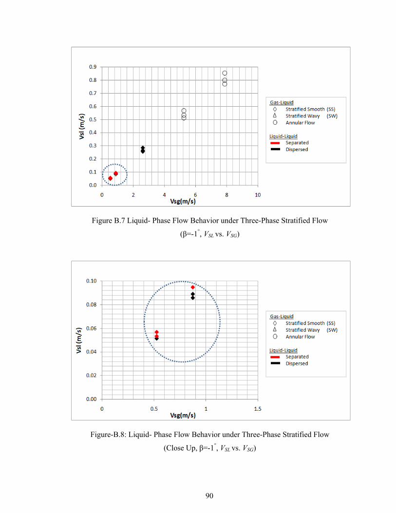
90

Figure B.7 Liquid- Phase Flow Behavior under Three-Phase Stratified Flow

(β=-1°, VSL vs. VSG)

Figure-B.8: Liquid- Phase Flow Behavior under Three-Phase Stratified Flow

(Close Up, β=-1°, VSL vs. VSG)

91

APPENDIX C

COMPUTER CODE FOR GAS-LIQUID SPLITTING (Case 2)

This section presents a computer code developed in this study for the prediction

of the gas-liquid splitting in looped lines, which is an extension of a unique experimental

study on gas-liquid splitting in parallel and looped lines carried out by Alvarez (2009).

C.1 Computer Code in Microsoft Excel Spread Sheet

The computer code was developed in an Excel spread sheet, which consists of

four screens. Figure C.1 shows the first of the four screens, namely, the input pipeline

profiles. Each flow line profile should be specified in the input profile screen by entering

length, inclination angle and diameter of respective flow lines. Schematics of flow line

profiles are generated automatically below the input profile tables of each flow line based

on the input data.

Figure C.2 shows the input flow condition screen. Total gas and liquid flow rates,

water cut and the specific gravities of oil, water and gas, outlet pressure and temperature

are specified in the input flow conditions screen.

92

Figure C.1 Input Profile Screen

Figure C.2 Input Flow Condition Screen

93

Several options exist for each fluid property as shown in Figure C.3. The

correlation list can be seen by clicking the arrows next to the PVT correlations. The

pressure drop method must also be selected from twelve pressure drop models and

correlations. The liquid specific heat, constant volume gas specific heat and isobaric gas

specific heat correlations were also added for further improvement of the program.

The code is based on a pressure drop balance, whereby the pressure drop in the

two looped lines should be equal to each other, this is due to the inlet pressure and outlet

pressure being same for both flow lines, owing to the looped lines configuration. Equal

GOR in both pipelines is assumed in this tool in order to solve the problem. Using the

solver application of Microsoft Excel and setting the pressure drop difference between

the flow lines equal to zero, convergence on the flow splitting in the looped lines can be

achieved. The program provides the inlet pressure, outlet pressure, pressure drop, flow

rate and fraction of gas, water and oil for each flow line. Figure C.4 shows the results

screen.

94

Figure C.3 Input PVT Correlations Screen

Figure C.4 Results Screen

95

C.2 Computer Code Predictions for Actual Field Data

The developed gas-liquid splitting computer code was run for a real field case,

case 2, provided by Chevron. Predictions of the study’s computer code were also

compared with OLGA simulation predictions for this case.

Figure C.5, Table C.1 and Table C.2 show the field data provided by Chevron.

Total gas and liquid is split into two flow lines, which are 6-in. and 8-in.-OD pipes

respectively. Each of the flow lines has the same profile, consisting of five different

sections. Table C.1 presents the coordinates of each section of the lines. The

configurations of the five sections are horizontal, downward vertical, downward inclined,

upward vertical and horizontal as shown in Figure C.5. In addition, the flow conditions

are given in Table C.2 in terms of the gas, water and oil specific gravities, total flow

rates, water cuts and separator pressures and temperatures.

Table C.3 shows a comparison between OLGA’s predictions and the developed

computer code predictions of gas and liquid splitting in the looped lines. The developed

computer code’s predicted that 31.47% of the gas and liquid flows in the 6 in. pipe and

68.53% of the gas and liquid flows in the 8 in. pipe. As shown in Table C.3, liquid and

gas fraction predictions show good agreement with the OLGA predictions and the

splitting predictions are almost equal for both methods. The small difference between the

gas fraction predictions is due to the constant GOR assumption of this study’s code.

96

Table C.1 Coordinates of Flow Line Sections

Figure C.5 Schematic of Flow Line Profile

X (ft) Y(ft)

0 0

169 0

169 -248

6796 -260.2

6796 -17.2

7005 -17.2

97

Table C.2 Chevron Field (Case 2) Flow Conditions

Table C.3 Comparison between the OLGA and Computer Code Predictions

Gas Specific Gravity 0.761

Water Specific Gravity 1.02

Oil Specific Gravity 32.2 API

Total Gas Flow Rate 1.3 MMscf/d

Total Liquid Flow Rate 25581 STB/d

Water Cut 46%

Separator Temperature 115 F0

Separator Pressure 85 psig

OLGA CURRENT STUDY

Diameter (in) 6" 8" 6" 8"

fliquid (%) 31 69 31.47 68.53

fgas (%) 27 73 31.47 68.53

T H E U N I V E R S I T Y O F T U L S A THE GRADUATE ... Orkun_Er_ Thesis _2010.pdf · the graduate...

Documents

Transcript of T H E U N I V E R S I T Y O F T U L S A THE GRADUATE ... Orkun_Er_ Thesis _2010.pdf · the graduate...