T DEMARCATION OF LAND AND THE ROLE OF · PDF fileTHE DEMARCATION OF LAND AND THE ROLE OF...
65
THE DEMARCATION OF LAND AND THE ROLE OF COORDINATING INSTITUTIONS GARY D. LIBECAP AND DEAN LUECK Abstract. This paper examines the economic effects of the two dominant land demarcation systems: metes and bounds (MB) and the rectangular system (RS). Under MB property is demarcated by its perimeter as indicated by natural features and human structures and linked to surveys within local political jurisdictions. Under RS land demarcation is governed by a common grid with uniform square shapes, sizes, alignment, and geographically-based addresses. In the U.S. MB is used principally in the original 13 states, Kentucky, and Tennessee. The RS is found elsewhere under the Land Ordinance of 1785 that divided federal lands into square-mile sections. We develop an economic framework for examining land demarcation systems and draw predictions. Our empirical analysis focuses on a 39-county area of Ohio where both MB and RS were used in adjacent areas as a result of exogenous historical factors. The results indicate that topography influences parcel shape and size under a MB system; that parcel shapes are aligned under the RS; and that the RS is associated with higher land values, more roads, more land transactions, and fewer legal disputes than MB, all else equal. The comparative limitations of MB appear to have had negative long-term effects on land values and economic activity in the sample area. July 16, 2009 JEL Codes: D23, K11, N50, O17, Q15 Libecap: University of California, Santa Barbara, [email protected] . Lueck: University of Arizona, [email protected] . Research support was provided by the National Science Foundation through grants SES-0518572 and 0817249; the Cardon Endowment for Agricultural and Resource Economics at the University of Arizona; and the International Centre for Economic Research (ICER), in Torino, Italy. We also acknowledge the exceptional research assistance of Trevor O’Grady, Adrian Lopes, and Sarah McDonald and other research assistants including Chris Brooks, Sean Small, Andrew Knauer, Maxim Massenkoff, and Andrew Smithey, as well as the staff at the Ohio State Library. Helpful comments were provided by Benito Arruńada, Roger Bolton, Karen Clay, Robert Ellickson, Joe Ferrie, David Haddock, Richard Hornbeck, Matt Kotchen, Sumner LaCroix, Anup Malani, Trevor O’Grady, Steve Salant, Steve Shavell, Henry Smith, Peter Temin, and Ian Wills as well as participants in the NBER (DAE) Summer Institute, 2008; the American Law and Economics Association Meetings, 2008; the International Society for New Institutional Economics Meetings, 2008; ASSA Meetings, 2008; the UCSB Occasional Conference on Environmental and Resource Economics, 2008; the Latin American and Caribbean Economics Association meetings, and seminars at Yale, Stanford, Michigan, Hawaii, UC Berkeley, UC Irvine, UCLA, Northwestern, Arizona, University of Chicago, Cornell, Oregon State University, Hong Kong Polytechnic Institute, and Peking University.
Transcript of T DEMARCATION OF LAND AND THE ROLE OF · PDF fileTHE DEMARCATION OF LAND AND THE ROLE OF...

THE DEMARCATION OF LAND AND THE ROLE OF COORDINATING INSTITUTIONS
GARY D. LIBECAP AND DEAN LUECK
Abstract. This paper examines the economic effects of the two dominant land demarcation systems: metes and bounds (MB) and the rectangular system (RS). Under MB property is demarcated by its perimeter as indicated by natural features and human structures and linked to surveys within local political jurisdictions. Under RS land demarcation is governed by a common grid with uniform square shapes, sizes, alignment, and geographically-based addresses. In the U.S. MB is used principally in the original 13 states, Kentucky, and Tennessee. The RS is found elsewhere under the Land Ordinance of 1785 that divided federal lands into square-mile sections. We develop an economic framework for examining land demarcation systems and draw predictions. Our empirical analysis focuses on a 39-county area of Ohio where both MB and RS were used in adjacent areas as a result of exogenous historical factors. The results indicate that topography influences parcel shape and size under a MB system; that parcel shapes are aligned under the RS; and that the RS is associated with higher land values, more roads, more land transactions, and fewer legal disputes than MB, all else equal. The comparative limitations of MB appear to have had negative long-term effects on land values and economic activity in the sample area. July 16, 2009 JEL Codes: D23, K11, N50, O17, Q15 Libecap: University of California, Santa Barbara, [email protected]. Lueck: University of Arizona, [email protected]. Research support was provided by the National Science Foundation through grants SES-0518572 and 0817249; the Cardon Endowment for Agricultural and Resource Economics at the University of Arizona; and the International Centre for Economic Research (ICER), in Torino, Italy. We also acknowledge the exceptional research assistance of Trevor O’Grady, Adrian Lopes, and Sarah McDonald and other research assistants including Chris Brooks, Sean Small, Andrew Knauer, Maxim Massenkoff, and Andrew Smithey, as well as the staff at the Ohio State Library. Helpful comments were provided by Benito Arruńada, Roger Bolton, Karen Clay, Robert Ellickson, Joe Ferrie, David Haddock, Richard Hornbeck, Matt Kotchen, Sumner LaCroix, Anup Malani, Trevor O’Grady, Steve Salant, Steve Shavell, Henry Smith, Peter Temin, and Ian Wills as well as participants in the NBER (DAE) Summer Institute, 2008; the American Law and Economics Association Meetings, 2008; the International Society for New Institutional Economics Meetings, 2008; ASSA Meetings, 2008; the UCSB Occasional Conference on Environmental and Resource Economics, 2008; the Latin American and Caribbean Economics Association meetings, and seminars at Yale, Stanford, Michigan, Hawaii, UC Berkeley, UC Irvine, UCLA, Northwestern, Arizona, University of Chicago, Cornell, Oregon State University, Hong Kong Polytechnic Institute, and Peking University.

Libecap & Lueck -- The Demarcation of Land
1
“The beauty of the land survey…was that it made buying simple, whether by squatter, settler or speculator. The system gave every parcel of virgin ground a unique identity, beginning with the township. Within the township, the thirty-six sections were numbered …, beginning with section 1 in the north-east corner, and continuing first westward then eastward, back and forth, …. And long before the United States Postal Service ever dreamed of zip codes, every one of these quarter-quarter sections had its own address, as in ¼ South-West, ¼ Section North-West, Section 8, Township 22 North, Range 4 West, Fifth Principal Meridian.” (Description of the American rectangular system in Linklater, 2002, 180-81) “Beginning at a white oak in the fork of four mile run called the long branch & running No 88o Wt three hundred thirty eight poles to the Line of Capt. Pearson, then with the line of Person No 34o Et One hundred Eighty-eight poles to a Gum on the So Wt side of the run corner to persons red oak & chestnut land.” (Description of parcel demarcated by metes and bounds from C.W. Stetson, 1935, 90). I. INTRODUCTION
The demarcation of land defines property boundaries and location and is a
foundation for land use and markets. Although it seems self-evident that a system of
demarcating rights to land will have long-term effects on land use and value, the literatures
in economics and in law have not addressed these issues.1 The two dominant demarcation
systems are metes and bounds (MB) and the rectangular system (RS).2 Metes and bounds is
found worldwide and is the default practice.3 Rectangular systems, however, are found in
large areas of the U.S. and Canada, as well as parts of Australia, and elsewhere.4 In the
1 We find no legal or economic scholarship on this topic and even major property law treatises (e.g., Dukeminier and Krier 2002, Merrill and Smith 2007) merely describe the dominant American system. Neither of the comprehensive treatises on law and economics by Posner (2002) and Shavell (2007) mentions land demarcation. Holmes and Lee (2008, 2009) make reference to spatial issues regarding land use, but do not examine the underlying demarcation structure. 2 The term ‘metes and bounds’ is primarily an English term although we use it to describe any decentralized, topography-based demarcation system. Geographers (e.g., Thrower 1966) use the term ‘indiscriminant’ survey. 3 Historically most land has been and is currently demarcated using indiscriminate or unsystematic systems like MB (Brown 1996, Estopinal 1993, Gates 1968, Hubbard 2009, Linklater 2002, McEntyre 1978, Price 1995, Thrower 1966). 4 The Romans actually extensively used a rectangular system called the centuria quadrata that was started in the 2nd Century BC. The Dutch also used rectangular systems in large drained areas. Both of these systems are still visible in modern European landscape. Libecap and Lueck (forthcoming) discuss these and other rectangular demarcation systems.

Libecap & Lueck -- The Demarcation of Land
2
U.S. the RS was established in the 18th century with the Land Ordinance of 1785, while
Canada and Australia both implemented the RS in the 19th Century.5
Under MB land is demarcated by natural features (e.g. trees, streams, rocks) and
relatively permanent human structures (e.g., walls, bridges, monuments). Parcels are
described independently by their perimeter and linked to a specific survey within a local
political jurisdiction. Individuals take little account of the spatial and temporal impacts of
their demarcation choices. Demarcation is vague, imprecise, and idiosyncratic. There are no
uniform addresses, boundaries, shapes, sizes, or alignments.
By contrast, under a centralized and coordinated RS, plots are described by a
geographically-based address that is part of a large, uniform grid of identical squares that
define shape, size, and (directional) alignment. This network communicates the precise
location of each parcel, even to those remote from the site. Boundaries are positioned to
avoid overlap and dispute and situated for the development of market roads along property
lines.
In this paper we exploit a natural experiment in land demarcation in Ohio that
provides us with an opportunity to examine MB and RS in adjacent areas and to compare
their effects on land markets. We examine counties within and adjoining the Virginia
Military District (VMD) in central Ohio, where land was demarcated by metes and bounds
and was (and still is) surrounded by land demarcated under the rectangular system. The
VMD was granted to Virginia in 1784, prior to settlement of the region and was governed
5Canada established the Dominion Land Survey in 1871. The RS began in Australia after 1834 in South Australia and after 1858 in Victoria See Crowley (1980), Jeans (1975), Priestly (1984), Powell (1970), and Williams (1974) for Australia; Taylor (1975) and Thompson (1967) for Canada; and Hubbard (2009) for the U.S.

Libecap & Lueck -- The Demarcation of Land
3
by MB under Virginia Law. The rest of Ohio was placed under RS by Congress following
enactment of the Federal Land Law in 1785. Ohio became a state in 1803.
We find that the coordinated RS resulted in more uniform parcel sizes, shapes, and
alignment, relative to individualized MB, where the perimeters, dimensions, and
positioning of tracts of land were far more variable and haphazard. In flat areas where
terrain we find that MB land parcels vary dramatically in shape, size and positioning with
respect to one another, compared to parcels under the RS. The standard deviation in the
number of parcel sides, reflecting differences in shape, is almost 4 times greater; the
coefficient of variation of parcel size under MB is almost twice that found in RS where
uniformity was the objective, and the standard deviation of parcel alignment is an order of
magnitude higher, revealing the differences in the configuration of parcels under MB,
compared to RS.
Additionally, topography factored heavily into the demarcation process under
individual, uncoordinated claiming with MB relative to demarcation under the RS, where it
played almost no role. Further, with unsystematic demarcation, property boundary and title
disputes were much more common under MB, with almost 18 times the conflict rate as in
RS regions during the 19th century. Lacking straight property boundaries for the
coordinated placement of roads, MB also retarded road investment. MB townships had over
24 percent lower road density than was found in RS townships, all else equal.
With regularly-shaped, sized, and aligned parcels as well as standardized property
descriptions and addresses, land markets were more active under RS. In our sample, there
were 50 percent fewer conveyances in MB counties. All of this lowered land values per

Libecap & Lueck -- The Demarcation of Land
4
acre under the MB by more than 10 percent, depending on the sample and whether
township or farm level data are used.
The distinction between these two land demarcation systems illustrates basic,
important differences in how institutions can coordinate economic activity. Our analysis
draws on the work of Coase (1960), Williamson (1975), Libecap (1989), Baird, Gertner and
Picker (1994), Dixit (2003), and Farrell and Klemperer (2007) on the roles of legal
institutions in expanding markets and coordinating economic activity. In doing so we
develop a framework that merges the economics of property rights with the economics of
networks.
The paper is organized as follows. We begin in section II with a brief history of the
U.S. land demarcation systems. In section III we develop an economic framework for
analyzing the demarcation of land under both metes and bounds and the rectangular survey,
and for analyzing the effects of the rectangular survey on land use, land markets, property
disputes and public land-based infrastructure. Section IV is an empirical analysis of land
demarcation, land markets, and property disputes. In Section V we summarize our findings
and discuss their implications.
II. A BRIEF HISTORY OF U.S. LAND DEMARCATION SYSTEMS
In the United States MB was inherited from England and is thus found in the 13
original states. It also exists in Kentucky, Tennessee, parts of Maine, Vermont, West
Virginia, and where Spanish and Mexican land grants were prevalent in Texas, New
Mexico, California, and Arizona.6 MB in the United States ended with the enactment of the
6 Louisiana recognized early French and Spanish descriptions, particularly in the southern part of the state, which has features of both MB and RS. Hawaii has a traditional indiscriminate system that can be classified as MB as well. Texas was not carved out of federal land, in non Spanish land grant areas, the state has its own system of rectangular surveys that are not linked to the U.S. system of meridians and baselines. Libecap,

Libecap & Lueck -- The Demarcation of Land
5
Land Ordinance of 1785 (Hubbard 2009).7 The law required that the federal public domain
be surveyed prior to settlement and that it follow a rectangular system. Land sales were to
be the primary source of revenue for the federal government, and the government bore the
initial costs of survey to provide a uniform grid of property boundaries that were standard
regardless of location and terrain. The RS applied to most of the U.S. west and north of the
Ohio River and west of the Mississippi north of Texas as indicated in Figure 1.
- FIGURE 1 HERE -
The American rectangular system uses a network of meridians, baselines,
townships, and ranges to demarcate land.8 The survey begins with the establishment of an
Initial Point with a precise latitude and longitude. Next, a Principal Meridian (a true north-
south line) and a Baseline (an east-west line perpendicular to the meridian) are run through
the Initial Point. On each side of the Principal Meridian, land is divided into square (six
miles by six miles) units called townships. A tier of townships running north and south is
called a “range.” Each township is divided into 36 sections; each section is one mile square
and contains 640 acres. These sections are numbered 1 to 36 beginning in the northeast
corner of the township.9 Each section can be subdivided into halves and quarters (or aliquot
parts).10 Each quarter section (160 acres) is identified by a compass direction (NE, SE, SW,
NW). Each township is identified by its location relative to the Principal Meridian and Lopes, and Lueck (2009) analyze the impact of the MB system on land values in the land grant areas of California. 7 See text at http://memory.loc.gov/cgi-bin/query/r?ammem/bdsdcc:@field(DOCID+@lit(bdsdcc13201) accessed June 28, 2009. It was replaced by the Land Ordinance of 1787, the Northwest Ordinance that allowed for larger individual allotments – see text at http://rs6.loc.gov/cgi-bin/ampage?collId=llsl&fileName=001/llsl001.db&recNum=173 accessed June 28, 2009. 8 Townships under the RS are grid locations. They are different from the political jurisdictions that are found in many U.S. counties. The RS system is officially known as the Public Land Survey System or PLSS; http://www.nationalatlas.gov/articles/boundaries/a_plss.html accessed June 30, 2009. 9 Some of the earliest surveys in the rectangular system had slightly different numbering systems but by the mid 1800s this system was in place (Hubbard 2009, Thrower 1966). Canada’s system uses a slightly different numbering system but also has 36 sections in a 6 by 6 mile township like the US system. 10 And urban developers may also subdivide into smaller parcels within this system.

Libecap & Lueck -- The Demarcation of Land
6
Baseline. For example, the Seventh Township north of the baseline and Third Township
west of the First Principal Meridian would be T7N, R3W, First Principal Meridian. In this
manner, properties are positioned relative to one another in a standardized way.
There are 34 sets of Principal Meridians/Baselines—31 in the continental United
States and 3 in Alaska, all shown in Figure 1. The rectangular system began with the first
survey in eastern Ohio on the Pennsylvania border at what is now called the Point of
Beginning (Hubbard 2009, Linklater 2002). Proceeding westward across the federal
domain, the system was made more uniform by establishing one major north-south line
(principal meridian) and one east-west (base) line that control descriptions for an entire
state or region. The meridians and baselines are defined by longitude and latitude.11 The
differences between MB and RS are summarized in Table 1.
- TABLE 1 HERE –
III. ECONOMICS OF LAND DEMARCATION SYSTEMS
We develop an economic framework for a comparative analysis of RS and MB by
first considering how land would be demarcated under MB. Next we consider the potential
gains from a centralized and coordinated land demarcation system that covers a large
region. Finally we analyze how the RS generates different ownership patterns and
incentives for land use, land markets, investment, and border disputes.
A. Individual Land Demarcation in a Decentralized System: Metes and Bounds
To start we examine a case in which non-cooperative agents claim and enforce
separate plots in order to maximize the value of their land, net of demarcation and
11 County lines frequently follow the survey, so most counties in the western two-thirds of the US that are highly linear and often rectangular. Individual properties tend not to overlap county boundaries in order to designate administrative jurisdiction and taxing authority See (Hubbard 2009, Libecap and Lueck forthcoming) on political jurisdictions and borders.

Libecap & Lueck -- The Demarcation of Land
7
enforcement costs. Consider a tract of land of A acres, whose external boundary is
enforced collectively or otherwise by a sovereign, so that individual decision makers
consider only internal and shared borders. Each claimant can only choose and demarcate a
single parcel. Within the external borders, there is no coordination or contracting among
claimants.12
In this setting each potential claimant chooses the number of acres to claim and the
length of boundary to enforce in order to maximize profits net of enforcement costs.13
Formally each claimant will solve
(1) ,
1
max ( , , ) ( , , )
. .i i
i i i i i i i i ia p
n
i i
V y a p t c a p t
s t a A=
= −
=∑
where ai is the area claimed (e.g., acres) by each of the n claimants; pi is the plot perimeter
(e.g., miles); ti is an indicator of the land’s topographical features (e.g., ruggedness) or land
quality; yi(ai,pi,ti) is the total value function that depends on the acres claimed, perimeter
(and implicitly, the parcel shape), and land characteristics; ci(ai,pi,ti) is a demarcation and
enforcement cost function that also depends on a, p, and t. The non-cooperative Nash
equilibrium solution to this problem is the optimal size (a) and perimeter (p) pair -- * *( , )i ia p -
- which implies a plot shape.
Consider the simple case in where claimants have the same productivity
( , )i jv v i j= ≠ , the same enforcement costs ( , )i jc c i j= ≠ , and value does not depend on
12 We ignore the optimal time to claim under first possession rules that are associated with an open access resource (Lueck 1995). Similarly we assume that a claimant obtains rights akin to fee simple (perpetual) ownership of the parcel and not just a one-time claim to a flow of output from the land asset. Also, it is likely that even with MB there are legal and social rules (e.g., custom, norms) enforcing the right to claim and define rights to land using geographic and topographic landmarks. 13 We lump demarcation and enforcement costs together though in practice there are likely to be distinctions such as costs of surveying, costs of maintaining fences for livestock, costs of observing intruders, and so on. We also assume that the claims are made simultaneously rather than sequentially.

Libecap & Lueck -- The Demarcation of Land
8
topography or shape. The problem for each party is to simply minimize the border
demarcation and enforcement costs, constrained by the productivity of the land. If the land
is perfectly flat, these costs might simply be c kp= where k is a parameter, so the question
is what perimeter, and by implication what shape, will minimize these costs for a give area?
Alternatively the question is what shape generates the largest area (and thus the lower
enforcement costs per area) for a given perimeter. Put this way, the question is the ancient
and famous isoperimetric problem.14
The answer to the isoperimetric problem is that a circle will maximize the area for a
given perimeter, providing the lowest perimeter to area (p/a) ratio. Consider a circular plot
with a four-mile perimeter. The area will be 4 / 1.27π = square miles and /p a π= .15 In
contrast, a square parcel with a four-mile perimeter will have an area of just one square
mile and / 4.0p a = .16 If enforcement costs simply depend on the perimeter or the
perimeter relative to area, we should see circular plots as a Nash equilibrium, rather than
squares.17 A more likely situation is that the total land constraint will be binding and a
pattern of circular plots will leave large areas of unclaimed land. In fact the unclaimed
corners in circular pattern amount to about 22 percent of the total tract.18 These unclaimed
14 See Dunham (1994) for history and analysis; also see http://en.wikipedia.org/wiki/Isoperimetry for an overview of this problem. In our notation the solution to the isoperimetric problem is the inequality 4πa ≤ p2
and only a circle will make the equality hold. The literature on the economics of location (e.g., Lösch 1954) develops a similar model in which the landowner’s objective is to minimize transportation costs to the central farm site. 15 The area of a circle is a = πr2 and the perimeter is p =2πr where r is the radius. 16 For a circle p/a = 2/r and for a square p/a = 4/s where s is the length of each side. 17 To our knowledge circular parcels are rare. Libecap and Lueck (forthcoming) discuss circular plots used in Cuba, which created many problems of overlapping claims and boundary disputes. The circular areas observed while flying across the Great Plains are due to irrigation equipment that pivot from a central point. 18 For a circle with a diameter of 1 mile the area is 0.785 square miles, or 21.5 percent less that a 1 mile square section. If you count the corners as 4 separate plots then the total perimeter of the circular plot and the corner plots is 7.142 miles compared to just 4 miles for a single square. This total is obtained from adding the perimeter of the circle (3.142 miles) to that of the square.

Libecap & Lueck -- The Demarcation of Land
9
open access areas would not only dissipate potential rents, but might create locales where
intruders could raise demarcation and enforcement costs.
Regular polygons are a possible alternative to circles as equilibrium parcel shapes
because they have the potential to eliminate unenclosed waste between parcels (a problem
for circles) and because they are likely to be more valuable shapes because of their linear
sides.19 Regular polygons maximize the area enclosed by a given perimeter and thus have
the lowest p/a ratio for any n-sided polygon (Dunham 1994). Further, there are only three
regular polygons – triangles, rectangles (squares), and hexagons – that can create patterns,
with a common vertex and have no interstitial space (Dunham 1994, pp.108-111).
The choice among triangles, squares, and hexagons can be explored by further
analysis of parcel perimeter demarcation and enforcement costs as well as the contribution
of shape to the value of output. The perimeter to area ratio (p/a) will be lowest for
hexagons, then squares, and finally triangles. Survey and fencing (enclosure) costs are
lower for plots with fewer angles and longer straight boundaries (Johnson 1976). This
clearly favors squares over triangles and hexagons. Finally, squares are more valuable for
agriculture land use because they allow for rectangular fields are more productively
efficient by eliminating redundant effort from excessive turns and travel in fieldwork and
simplifying calculations for seeding and harvest.20 The combination of these factors leads
to our first prediction:
19 A regular polygon is a polygon with all sides the same length and all angles the same. The sum of the angles of a polygon with n sides, where n is 3 or more, is 180(n - 2) degrees. A triangle comprises 180 degrees, a square 360 degrees, and so on. 20 Studies by Barnes (1935), Lee and Sallee (1974), and Amiama, Bueno, and Alvarez (2008) show production advantages in rectangular fields where the operator works parallel to the longest sides of the field. Johnson (1976, 153) describes 19th Century farming, showing why rectangular fields were optimal.

Libecap & Lueck -- The Demarcation of Land
10
Prediction 1: With homogeneous (flat) land and homogeneous parties (in both productive and enforcement ability) a decentralized (uncoordinated) metes and bounds system will yield a land ownership pattern of identical square parcels.
If demarcation and enforcement costs (surveying-fencing-policing) and land value
depend on terrain, borders will roughly follow topography. We expect the non-cooperative
Nash equilibrium to yield a pattern of parcel sizes and shapes that depends on the character
of the land (e.g., topography, vegetation, soil quality) and of the potential claimants
(farming productivity, violence and monitoring productivity).21 Thus:
Prediction 2: With heterogeneous land and parties (in both productivity and enforcement ability) a decentralized (uncoordinated) metes and bounds system will yield a land ownership pattern of parcels whose borders mimic the topography and vary in size with no particular alignment.
B. Land Demarcation a Centralized Rectangular System
It is apparent that there are potential gains from centralized demarcation (Hubbard
2009). First, there can be enforcement cost savings from coordinating common borders,
eliminating gaps and gores. Second, similarly aligned properties will eliminate odd-shaped,
unproductive parcels that arise with unsynchronized demarcation of large areas. A
common alignment of parcels (e.g., north-south) requires either a strong social convention
or centralized authority.22 Third, a coordinated survey of heterogeneous land prior to
allocation fixes individual parcel borders and sizes, and precludes the incentives of agents
to “float” boundaries to cover the most productive land. Such opportunistic border
adjustments could result in costly, long-term boundary disputes among adjacent properties
as new information is revealed about land productivity.23 Fourth, a common demarcation
21 With heterogeneity agents enclose will only the best land and leave unclaimed areas -- the so-called ‘gaps and gores’ described by many historians of MB systems. 22 Sugden’s (1990) theory of conventions is based on repeated games which have little application for a MB system where claimants do not repeat the interaction. 23 Clay and Wright (2005) describe the process of moving or floating claims to mineral land during the early

Libecap & Lueck -- The Demarcation of Land
11
pattern provides information about the position of individual parcels. This information
reduces potential for overlapping and conflicting claims; allows for a common address
system; and importantly, lowers transaction costs, promoting land markets. Hence,
coordinated demarcation is a public good network that will have greater value as it is
spread over a large region.
The economic decision to adopt a centralized RS can be examined by comparing the
total value of land under both arrangements, which is the sum of parcel values less the costs
of the systems themselves. To do so, assume the region governed by a system is A acres,
split into n parcels, each of size a, so that A = na. In addition we incorporate a temporal
dimension to account for difference in system setup and continuation costs.
Under MB the net value of the land is the sum of individual values and costs, less
the continuing costs associated with adjustments resulting from the lack of coordination, so
that the total present value of the land in the region is
(2)
( ) 010
( *, *; ) ( *, *; ) ( , *; )T n
MB MB ri
iv p a t c a p t C A a t e dV ττ τ τ−
=
⎛ ⎞= − −⎜ ⎟⎠⎝
∑∫ ,
where * * *( , ; )i iv v p a tτ τ= is the optimal parcel value under MB at time τ, T is the time
horizon, r is a discount rate, c0(a*,p*;t) is the one-time demarcation cost function, and
( , *; ) 0MBC A a tτ ≥ are the continuing costs of MB as described above, including individual
enforcement, border disputes, and misaligned parcels. Under MB land demarcation and
output begin immediately at time τ = 0 and the continuing costs associated with MB are
assumed to be increasing in the size of the region (A) and rising over time (τ) as these
problems accumulate.
California gold rush when the location of ore was uncertain. During this initial period mineral claims were uncoordinated under MB.

Libecap & Lueck -- The Demarcation of Land
12
Unlike MB, RS is a coordinated framework, and the net value of land reflects its
results. Following Farrell and Klemperer (2007), we assume the network effects of RS are
such that a person’s or group’s use benefits others and that it further increases the incentive
of others to use the system.24 The network benefits are the public goods of common
addresses, survey coordination, and standardized, aligned and fixed parcel boundaries.
These network and coordination benefits come, however, at the cost of a necessarily
extensive system.25 Under RS there are upfront costs of design, survey, and controlling
access until demarcation is completed.
Individual land claimants within RS are assumed not to face demarcation costs as
with MB. There are only system costs to consider. Under these assumptions the total
present value of the land in the region governed by RS is
(3) ( )'
1' 0
( , , ; ) ( , ; ) ,T n
RS r RS ri
iv a p n t e d C A a t e dV
ττ τ
τ ττ τ
τ τ− −
= =
⎛ ⎞= −⎜ ⎟⎠⎝
∑∫ ∫
where ( , , ; )i iv v p a n tτ τ= is the optimal value for parcel i under RS at time τ where
/ 4.0p a = under the structure of squares; T is the time horizon, r is a discount rate;
( , ; ) 0RSC A a tτ ≥ is the cost of the system that occurs prior to claiming and use. Network
effects are incorporated into the parcel value function, which is increasing in the number of
parcels governed by the RS, where /n A a= .26 RS system costs are increasing in A, but at a
decreasing rate, revealing network economies. These costs are also increasing in
24 Farrell and Klemperer (2007) use the term ‘adoption’ as they are concerned with a firm’s decision to choose a new good with network effects. Baird, Gertner and Picker (1994) discuss how legal institutions (e.g., provide information, coordinate agents) can solve collective action problems. 25 Our MB – RS cost distinction is similar to Dixit’s (2003) distinction between local (informal) and large (formal-legal) trading systems, where the latter have greater setup costs like RS. 26 We ignore the optimal choice of square parcel size and take it as a constraint that is consistent with our understanding of the American RS.

Libecap & Lueck -- The Demarcation of Land
13
topography.27 Because RS requires surveying before parcel selection, the time horizon for
generating value from the land begins at τ’ > 0.
It is efficient to implement RS when RS MBV V− > 0 and some predictions can be
generated under simplifying assumptions. First let nii
V v=∑ and * *nii
V v= ∑ to simplify
notation. Second, assume that the land is flat (t = 0) and that the RS parcel shapes and sizes
are the same as would be chosen under decentralized MB ( *, *)a a p p= = then
(4) )( )('
* *0
' 0 0
( ) .T T
RS MB r RS r MB rV V V n V e d V C e d c C e dτ
τ τ ττ τ τ τ
τ
τ τ τ− − −− = − − + + +∫ ∫ ∫
This difference has four terms that illustrate the tradeoffs between RS and MB. The
first term comprises the network gains from RS over MB. The second term is the gains
from MB that would be sacrificed during the period the RS is being implemented, in terms
of output under MB and RS setup costs. The third term is the foregone individual
demarcation costs under MB not required under RS, and the fourth term is the avoided
continued costs of MB over the time horizon. From (4) comparatives statics emerge: the
net value of RS will increase in the size of the governed land area (A), increase in the
expected time horizon (T), and decrease in the time of RS implementation (τ). This leads to
the following predictions:
Prediction 3. A rectangular system is more likely to be adopted when a) agents (e.g., national governments, land companies, suburban developers) can control large tracts of land, b) when the time horizon is longer, and c) when implementation can be rapid.
Considering forces likely to change the model parameters can illuminate these
predictions. For instance, more rugged topography would reduce net gains from RS by
27 These effects are greater than with MB because squares are required.

Libecap & Lueck -- The Demarcation of Land
14
increasing the costs and time of RS implementation and perhaps even by reducing the
losses of sub-optimal parcel shape.28 Similarly one might expect that a region where no
incumbent demarcation system existed would lower RS implementation costs.29 Finally,
political authority and stability will increase the expected time horizon and make RS
adoption more likely.
The structure of the RS value function in (3) has economic implications for land
markets once RS has been adopted. Because parcel boundaries are standardized and
aligned, there are fewer overlapping borders and unclaimed gaps outside property
descriptions.30 These factors imply another prediction:
Prediction 4: There will be fewer legal disputes (and litigation) over boundaries and titles under the rectangular survey than under metes and bounds.
RS lowers the cost of using the market, thus allowing plots to be reorganized as
market conditions change (Barzel 1982). This should be observed as a greater number of
transactions, such as mortgages and conveyances per unit of land than under MB. This
should also increase the value of land and lead to more uniform sizes and shapes of parcels
in a region. For example, in a competitive market with access to a common technology,
farms within homogeneous regions should be similarly sized and shaped.31 This discussion
leads to three related predictions:
28 It is possible that had the federal frontier been comprised of very mountainous terrain across the continent rather than the Great Plains that the RS might not have been adopted in a broad scale. In areas of extremely rugged terrain forcing a square grid on the landscape could lead to high costs for surveys, fence lines, and roads (Johnson 1976, 19). MB boundaries tend to avoid such areas, lowering those costs. 29 Although we observe the purchase of agricultural lands for subdivision into suburban lots we do not observe large scale reorganization of agricultural MB properties into RS. The value of the added gains may not be sufficient to offset the uncertainty associated with the productivity of land to be included in any reconfigured property. Agricultural lands typically are consolidated into larger holdings rather than subdivided as with urban lands. 30 See Priest and Klein (1984) who similarly argue that uncertain legal rules result in more litigation. 31 Even though the original plots are square, consolidation under RS might lead to combinations of rectangles as the plots are subdivided into quarter sections and so on.

Libecap & Lueck -- The Demarcation of Land
15
Prediction 5: (A) There will be less variance in the size and shape of parcels under RS than MB. (B) There will be more land transactions under the rectangular survey than under metes and bounds. (C) There will be higher (per acre) land values under the rectangular survey than under metes and bounds. The coordinated clarity of RS is also expected to have an impact on public
infrastructure, such as roads that require long rights-of-way. Contiguous linear borders
should lower the cost of assembling rights of way along parcel boundaries.32 This
implies another prediction:
Prediction 6: There will be more roads per unit of land under the rectangular system than under metes and bounds.
All of these predictions will be tested in the following section using a combination of
statistical data and historical accounts.
IV. EMPIRICAL ANALYSIS
In this section we test our predictions against a wide variety of data taken primarily
from 19th Century Ohio where historical events created a landscape in which an area of MB
demarcation is surrounded by RS demarcation. The source of this exogenous institutional
setting lies in the early history of American public land policy. The historical record and
available data from the Virginia Military District (VMD) and the surrounding region clearly
show that the two demarcation systems can be treated as a natural experiment, allowing us
to analyze the economic effects.
The analysis begins with an examination of the demarcation of land under MB in
the VMD in order to test Predictions 1 and 2 that posit a relationship between topography
and parcel demarcation. Next we present a historical analysis of the adoption of large
rectangular systems as a test of Prediction 3. We then examine legal disputes over
property title and boundaries in the Ohio courts (Prediction 4). Next we examine 32 Johnson (1976, 167) discusses the value of straight roads and benefits for surveyors and civil engineers.

Libecap & Lueck -- The Demarcation of Land
16
Predictions 5A-C that focus on the effects of land demarcation systems on land markets and
roads as local public goods (Prediction 6). The section ends with estimates of the net gains
from RS demarcation for our sample area.
A. Ohio and the Virginia Military District: Exogenous Land Demarcation Systems.33
The state of Ohio was created in 1803 out of the Northwest Territory, the first part
of an extensive public domain held by the United States government. It was comprised of
11 large land areas opened separately for survey and settlement by Congress.34 Some of
these were sold directly to large land companies or speculators, such as the 1787 Symmes
Purchase of 248, 250 acres in the southwest and the 1788 Ohio Company Purchase of 1.5
million acres in the east. Others such as Congressional Lands were surveyed and sold in
somewhat smaller allotments by Congress to developers and settlers.35 A third area, the
U.S. Military District, in the center of the state, was reserved in 1796 to compensate federal
veterans through the issuing of land warrants to soldiers with land grants varying according
to rank. Typically, veterans sold these warrants to land developers, who then transferred
them to actual settlers.36
The Virginia Military District (VMD) was another of these land areas. Prior to the
creation of the federal domain, colonies, and later states, had claims to western lands.
Virginia had one of the largest, based on its 1609 colonial charter from England ranging to
the Mississippi River and into the Great Lakes region (Hubbard 2009). Virginia agreed to
cede much of its claims north of the Ohio River in return for retention of a large tract of its
33 Hubbard (2009) provides a detailed history of this period and the demarcation of land. 34 These areas are shown in http://lib.oh.us/evolution/index.html and discussed in Knepper (2002). 35 Federal land authorizations often prescribed minimum-sized allocations. For example, from 1785-86, land was sold by the federal land office in plots of 640 acres. 36 Warrants in the U.S. Military District granted major generals 1,100 acres and solders 100 acres. As noted, most veterans sold their warrants, often to large developers. Indeed Knepper (2002, 41) finds that of the 1,043,460 acres covered by the warrants, just 22 people patented nearly 600,000 acres.
Libecap & Lueck -- The Demarcation of Land
17
choosing and in 1784 was granted the VMD. The area Virginia selected was a triangular-
shaped region of 4.2 million acres land along the northern border of the Ohio River,
between the Scioto and Little Miami Rivers.37 As with the U.S. Military District, this land
was to be used to compensate Virginia’s veterans through the granting of land warrants
according to a formula that gave larger acreages to those with higher rank and longer terms
of service (Hubbard 2009).38 As elsewhere in Ohio, these warrants were then sold to
individual migrants, land developers, or speculators.39
Indeed, the major objective for all of the Ohio lands was their ultimate transfer to
actual agricultural settlers. Migrants to the state were substantially the same, immigrating
from the Northeastern U.S., the South, and by 1840, from Germany.40 And for the most
part, the state’s terrain, soil, and climate were quite similar.
All of the lands in Ohio, except those in the VMD, were distributed under the
Federal Land Law of 1785 that required demarcation under the new rectangular system.41
Under the RS, an initial point was chosen and then two controlling survey lines were
established, a (principal) meridian and accompanying baseline. The land was surveyed,
often marking out boundaries of the townships with monuments or notches on trees to
establish the grid. In Ohio the surveys were conducted both by private parties and
government surveyors, but later government surveyors dominated. Land was then sold to
individuals or land companies, sometimes in large blocks, but always in square units. All of
37 The state of Ohio comprises 26.5 million acres so the VMD is roughly 16 percent of the state’s area. 38 Once a certificate of rank and service was presented to a court of law in Virginia for authorization, the Virginia Land Office in Richmond issued a warrant, either to the veteran or his heir or assignee. 39 This meant that land was quickly transferred into the hands of those who had a comparative advantage in using the land and not held by veterans who were often not familiar with the Ohio land or its use. 40 See http://lib.oh.us/evolution/regions/vamd.html for migration patterns in Ohio accessed on June 28, 2009. 41 The RS system varied somewhat in its early years, but the general practice across Ohio was consistent (Hubbard, 2009, Knepper, 2002, Pattison 1957, White 1983). Hubbard (2009) discusses the evolution of the RS. This experimentation with the early RS biases our statistical results against finding a positive RS effect.
Libecap & Lueck -- The Demarcation of Land
18
the land within each square was included in the sale, regardless of quality, making it
impossible to leave gaps and gores of unclaimed land under the RS. Any large blocks
generally were subdivided into half, quarter, or 1/8th sections (320, 160, or 80-acre plots)
and sold.
In contrast, VMD lands were demarcated under metes and bounds as practiced in
Virginia. In the VMD, purchasers could claim land by making an “entry” or “location” and
marking its perimeter on trees and other natural or human monuments (Thrower 1966, 43).
Unlike the requirements elsewhere in Ohio under the RS, the land entry did not have to be
contiguous; could be of virtually any shape; and could be split into multiple plots to cover
only the best lands. The entry was then described in a “call” filed at the local land office,
often the county seat. Once the entry and call were recorded, the claimant then hired a
surveyor to survey the claim’s boundaries and calculate the size of the entry. Upon filing
the survey at the land office, title or patent was granted.
Thus, as a result of exogenous Congressional actions regarding the distribution of
Ohio lands, the two major demarcation systems came to govern adjacent and nearly
identical lands and can be viewed as separate, imposed institutions: MB in the VMD and
the RS in the rest of Ohio. For our study, in order to control for other factors as much as
possible, we will constrain the analysis to the VMD and adjacent counties. The two maps in
Figure 2 show the location of the VMD within Ohio, as well as the neighboring counties.
- FIGURE 2 HERE -
Our primary region of analysis comprises 39 of Ohio’s 88 counties: 8 counties lie
wholly within the VMD and 5 additional counties have 50 percent or more of their territory
in the region. Of the 26 counties that surround the VMD, 17 are completely outside it and 9

Libecap & Lueck -- The Demarcation of Land
19
have less than 50 percent of their territory within the VMD. Table 2 provides comparative
statistics on various natural and economic characteristics for the VMD and surrounding
counties. In the table, VMD counties are those with at least 50 percent of their area within
the VMD and the remaining counties make up the surrounding counties group. The table
shows that the VMD and adjacent counties are virtually identical except for their land
demarcation systems. Indeed, we cannot reject the null hypothesis that two areas have the
same land characteristics (e.g., soil quality, terrain ruggedness, stream density) and initial
patterns of human settlement (e.g., place of birth, occupation). As shown, VMD lands have
slightly higher quality, are somewhat flatter, and have lower stream density (less swampy)
than the neighboring RS lands.42
- TABLE 2HERE –
B. Data and Empirical Strategy
The data used in the analysis are described in the Data Appendix, available on
request. Observations include information on land use outcomes (e.g. land values,
conveyances, roads), demarcation systems (MB or RS), original parcel characteristics (e.g.
shape, size, alignment), natural parameters (e.g., topography, soils, river density), and
economic parameters (e.g., market distance, population, roads). The data are at the
individual farm, original parcel, township, and county levels and are from the U.S.
population and agricultural census schedules, various Ohio state records, and Ohio court
opinions for the 19th Century, as well as contemporary USGS and USDA measurements.
Original parcels refer to very early land holdings that appear often to have been
42 Because Virginia chose the VMD prior to the implementation of the RS it is likely that the land was perceived of higher quality than adjacent territory which Virginia might have alternatively chosen. This selection bias would actually make estimates of the effects of land demarcation biased against the rectangular system.

Libecap & Lueck -- The Demarcation of Land
20
subsequently subdivided and sold. They do not generally correspond to farms as recorded
in the 1850 or 1860 censuses.43
Our focus on the early period of settlement allows us to examine land demarcation
effects in a relatively simple economic setting where the institutions differ at their points of
origin. Table 3 shows the variable definitions and summary statistics for the six different
data sets used in our empirical analysis.
1. Data.
Part A of Table 3 presents summary statistics for the 153 townships that are found
within the VMD. This sample is used to estimate the shape, size, and alignment of the
parcels demarcated under MB. Parcel shape data come from a digitized a map of early land
subdivisions in Ohio as chronicled by Sherman (1922). We have two measures of shape,
perimeter-area ratio and number of sides. The perimeter-area ratio comes directly from our
model and is measured as p/√a to keep units comparable. A perfect square would have a
value of 4.0 and the data show a township mean of 4.64, and the minimum value of 4.06 is
close to a square. Parcel sides (s) come from the same digitized database. The data show a
mean of 5.97 and a minimum of 4.08, again close to a square. These data indicate that even
under MB some townships had parcels with shapes that on average are nearly square.
Alignment variation captures the effects of ruggedness in disrupting parcel
placement when individuals were free to position their property. Parcels that are perfectly
aligned on a north-south axis imply a standard deviation of alignment to equal zero. We 43 The data appendix describes the variables that are used in the analysis. Sherman (1922) mapped “original” parcels and these have been digitized. Original parcels were not the initial purchases from the federal government or Virginia, which often were much larger as described in the text. They probably were the earliest subdivisions of those properties. Generally, they appear to be larger than most farms included in the census, suggesting that they were subdivided further. This process of subdivision was similar in both MB and RS areas as part of widespread land speculation on the agricultural frontier, but under the MB original parcels could be of any shape and alignment as compared to those in the RS that had to conform to its requirements for squares.

Libecap & Lueck -- The Demarcation of Land
21
see that this is generally not the case in VMD townships, as the mean of the sample shows a
standard deviation of alignment of 10.5 degrees. This is slightly lower than 13, the
standard deviation we would expect if the position of parcels was completely random.44 In
contrast, the maximum value of 18.3 is greater than 13. This suggests that some townships
may have homogenous parcel alignment within smaller groups, but a relatively sharp
contrast in alignment between groups. The size data in the table reveal that early parcels
were relatively large in the VMD, ranging from 139 acres to nearly 2,500 acres. Finally,
topography is measured by RUGGEDNESS, an index measure of slope, varying from 0 (flat)
to 1 (perpendicular cliff). As shown by the values in the table, there is terrain variation, but
the VMD is relatively flat.
- TABLE 3 HERE –
Part B summarizes data from 437 townships in the 39-county VMD region. We use
these data to estimate parcel alignment, shape, and size differences as well as road densities
in the two demarcation systems.45 In this dataset and most others, we measure demarcation
as the fraction of the jurisdiction governed by MB (i.e., % VMD). The table shows on
average 31 percent of township area in the sample is under metes and bounds. RUGGEDNESS
for the region is presented, again revealing how comparatively flat the entire area is, as well
as various measures of distance to markets. Cincinnati was the principal urban area to the
southwest and county seats typically were the major local market towns. Distance to
railroads and major waterways and road density reflect access to transportation options.
44 Since we do not expect any single alignment angle to be more likely than another, we assume alignment angles follow a continuous uniform random distribution with the range [0,45]. The standard deviation of this distribution is 12.99. 45 Number of parcels per township: MB — mean = 36, std = 225; RS—mean = 46, std = 58. Parcel size: MB – mean = 813, std = 611; RS – mean = 637, std = 113.
Libecap & Lueck -- The Demarcation of Land
22
Part C summarizes the data sample from the 437 townships in the 39-county VMD
region. There are 768 observations, which are mean township values for individual farmer
entries in the 1850 and 1860 manuscript censuses.46 These data are used to estimate land
values and include all the township variables shown in part B as well as variables on land
quality (PRIME FARMLAND) and demographics (LANDOWNER AGE, VIRGINIA BORN). All
farmland value data are in 1860 dollars, and the mean value is $35.37 per acre.47
Part D summarizes a sample of data from 39 counties in the VMD region and is
used to estimate land transactions as measured by mortgages and conveyances, reported by
the State of Ohio in 1858 and 1859. We report the mean values for those two years by
county, and on average there were 678 mortgages and 288 conveyances. The 1860 Census
reports an average of 1,925 farms per county.48 In addition to demarcation and topography
we also include data on the agricultural market (e.g., number of farms, farm acreage, farm
value).
Part E summarizes a sample of data from 456 farms from Warren County that is
used to estimate land values in a small, relatively homogenous area split into MB and RS.
These data are from 1867 farm maps of Warren County matched with 1870 Census
information to give the most micro level information on the impact of demarcation on land
value.49 Because we can determine whether or not a farm is in the VMD, a dummy variable
46 1850 is the first year the US Census contains detailed information on agriculture. We sampled both 1850 and 1860 censuses and matched agricultural and population census entries for both years. There are 3,938 matched individual observations in 1850 and 2,800 in 1860. We then calculated township mean values for the 437 townships in the VMD region for 1850 and 1860. As the appendix notes some 1860 census data has been lost for certain townships. As a result rather than having 874 observations (437x2) we have 768. 47 Number of Observations: (1850) MB – 123, RS – 289; (1860) MB – 120 RS – 242. Mean Number of Farms per Township Average: (1850) MB – 10.7, RS – 9.4; (1860) MB – 7.0, RS – 7.8. Farm Size (acres): (1850) MB – mean = 173, std = 235; RS – mean = 130, std = 59. (1860) MB – mean = 157, std = 235; RS – mean = 130, std = 59. 48 The reported averages for counties governed (in majority) by MB and RS are 1,817 and 1,978 respectively. 49 An 1867 plat map of farms with farmer names in Warren County (A. Warner, Philadelphia—see data

Libecap & Lueck -- The Demarcation of Land
23
is used for land demarcation. In our sample 42 percent of the farms are in the VMD and
thus governed by MB. Most of the independent variables are the same as in Part C,
although actual farm observations. RUGGEDNESS is the township value where the farm is
located.
2. Empirical Strategy.
We follow a consistent empirical strategy to identify the determinants of parcel
demarcation under MB and to identify the effects of demarcation (MB versus RS) on
economic outcomes.
The estimating equation for analysis of the impact of terrain on demarcation in the
VMD is
(5) yi = αi + Riβ + εi,
where yi measures average shape, size, or standard deviation of alignment for parcels in the
ith township; Rs is township i RUGGEDNESS; β is an unknown coefficient; and εt is a random
error term.
For the estimates of land use outcomes we use various tests so the specific level of
aggregation and set of variables depend on the samples. For example, for township-level
analysis we use township averages and the fraction of township land within the VMD to
denote land demarcation. The basic estimating equation is of the following form:
(6) yi = αi + Xiβ + MBiθ + εi,
where yi is an outcome measure (e.g., land value, conveyance, road density) for the ith
observation (parcels, townships, counties); Xi is a row vector of exogenous variables (e.g.,
land quality, topography, market variables), and a slope coefficient β is a column vector of
appendix) was matched to the 1870 agricultural and population census manuscripts for Warren County.

Libecap & Lueck -- The Demarcation of Land
24
unknown values; MBi is the land demarcation variable (VMD) for observation i, θ is an
unknown coefficient; and εs is a random error term. For market activities, our predictions
imply that θ < 0, or that MB will reduce outcome values such as land values, land
transactions, and road density. We estimate (5) and (6) both using OLS and techniques that
correct the standard errors for spatial dependence.50 When using aggregate data (e.g.,
townships) we weight the values by the number of parcels in the township or by fraction of
farmland in the relevant county.
C. Land Demarcation under Metes and Bounds in the Virginia Military District
Predictions 1 and 2 state that under MB the demarcation of parcels will depend on
the topography of the land. In relatively flat, homogeneous terrain we predict squares, and
in relatively rugged terrain, where land is heterogeneous we predict that the parcel shapes,
sizes, and alignment will follow local features, such as ridges and rivers that influence the
costs of demarcation c(p/a;t) and the (productivity) value of the land v(p/a;t). We test these
predictions by estimating the relationship between the topography of the land and the size,
shape, and alignment of the original MB-determined parcels in the VMD. For comparison
with RS, we also expand the sample to include townships in the adjacent counties. We
anticipate greater variation in size, alignment, and shape in the VMD because there are no
constraints on size, shape, and alignment as with the RS.
1. Size, Shape, and Alignment of Parcels within the VMD.
We begin the analysis with visual inspection of topography and parcel size and
shape within the central VMD. Figure 3, Panel A shows a section of flat land in Highland
50 We use Conley’s (1999) cross-sectional model that corrects for spatial dependence of an unknown form. This model assumes that spatial dependence will decline as the distances between observations increases. Without having information on the nature and potential causes of spatial correlation in our study, Conley’s spatial error model is appropriate.

Libecap & Lueck -- The Demarcation of Land
25
and Clermont counties.51 It is evident that the parcels are rectangular and even square as
predicted. As we noted above, there were large areas of land that had been assembled by
speculators who purchased warrants from veterans. The pattern shows evidence of
coordinated surveying, where groups of tracts are aligned in the same directions, but not
typically north-south as in the RS. This pattern is consistent with Prediction 3 regarding
the incentives to provide systematic demarcation when large tracts of land were owned.
Because we do not have detailed information about the first purchases of land for the VMD,
we cannot directly test the prediction that larger landowners more often implemented a
coordinated survey. Outside a particular large tract, however, surveys run in different
directions, and whenever groups of coordinated parcels abutted one another, the
configurations clashed, resulting in oddly-shaped and perhaps, unusable plots of land.
- FIGURE 3 HERE –
In contrast Panel B shows a similarly sized area in Pike County (eastern VMD)
where the terrain is more rugged. 52 Here the parcels tend to have much more variation in
parcel shape and size, with the boundaries often following land contours and other natural
features. There is no evidence of coordinated parcel boundary alignment in some areas as
seen in Panel A.53
- TABLE 4 HERE –
To further test predictions 1 and 2 we estimate (5), using data from 153 townships
in the VMD (Table 3, Part A). The estimation results are presented in Table 4. We expect
51 In Highland County the mean value for RUGGEDNESS is 0.027 and the standard deviation is 0.03; for Clermont County the mean is 0.034 and the standard deviation is 0.43. 52 In Pike County the mean RUGGEDNESS is 0.088 and the standard deviation is 0.067. 53 The major scholar of Ohio lands, William Peters (1930, 30, 135) pointed to the many gaps of vacant land found between parcels in the VMD. He noted that by 1852 when all military warrants had been used for land claiming, 76,735 acres of land remained unclaimed. To find some legal use of the properties, An Act of Congress transferred un-located and un-surveyed land in the VMD to the state of Ohio in 1871.
Libecap & Lueck -- The Demarcation of Land
26
that under MB parcel shape will tend to deviate more from a square, adding more sides, and
that the perimeter-area ratio will become larger as the land becomes more rugged. As
shown in all specifications terrain RUGGEDNESS has a statistically significant positive effect
on the average parcel perimeter-area ratio, number of sides, and standard deviation of
alignment within the VMD townships. RUGGEDNESS also has a significantly negative effect
on average parcel size. To illustrate, we compare the predicted parcel characteristics with
RUGGEDNESS at its mean and maximum values from our sample.54 This change increases
the average number of parcel sides from 6.6 to 9.2; the perimeter-area ratio from 4.8 to
5.9;55 and the standard deviation of alignment from 11.3 to 14.6. It also reduces the average
parcel size from 585 to 160 acres. These results suggest that as predicted under MB,
property boundaries and size are molded by topography. As the land deviates from flat
terrain, parcel shapes become less and less like squares; more haphazardly positioned; and
more variable in size.
2. The Effect of Demarcation System on Size, Shape, and Alignment of Parcels: MB vs. RS.
To examine the effects of the demarcation systems on parcel shape, alignment, and
size we modify (5) and estimate the following equation:
(7) yi = αi + Riβ1 + %VMDβ2 + (%VMD*R)iβ3+ εi
where yi is the standard deviation of parcel alignment, coefficient of variation of parcel
size, or standard deviation of our two parcel shape measures for the ith township; Ri is
RUGGEDNESS for township i; β is an unknown coefficient; VMD is the portion of the
township area under MB, and εt is a random error term. We use data from all 437 townships
54 In general, our sample is of rather flat terrain. The mean value is 0.025 and the maximum is 0.141. 55 For an 841-acre parcel (the sample average), perimeter-area ratios of 4.8 and 5.9 translate into boundary perimeters of about 5.5 and 6.2 miles respectively.

Libecap & Lueck -- The Demarcation of Land
27
in the 39 counties within and adjacent to the VMD (Table 3, part B). We anticipate that
parcels under MB will have a larger standard deviation of shape and alignment and a
greater coefficient of variation of size compared to a coordinated RS.56 We also expect
RUGGEDNESS to amplify these effects within MB areas where agents were not constrained
in the configuration of their parcels, as was the case within RS areas. Accordingly, we
include an interaction term. The estimates are reported in Table 5.
- TABLE 5 HERE –
The estimated coefficients for the VMD variable are positive and significant at the 1
percent level. By setting RUGGEDNESS equal to zero we can interpret the impact
demarcation systems have on shape, alignment, and size in flat terrain.57 We find the
standard deviation of the parcel perimeter-area ratio is more than doubled under MB; the
standard deviation of the number of parcel sides is almost 4 times greater; the standard
deviation of parcel alignment is an order of magnitude higher; and the coefficient of
variation of parcel size under MB is almost twice that in RS.
We also generally find a positive effect for the interaction term as predicted.
Because an interaction term is present, the effects of the demarcation system and
RUGGEDNESS are conditional on the value of the other variable. We can interpret the effect
that RUGGEDNESS has on shape, alignment, and size in the RS and MB by setting the VMD
variable equal to zero and one respectively. RUGGEDNESS has no statistically significant
impact on the variation of parcel shape or size under RS, although there is evidence that it 56We use the coefficient of variation instead of the standard deviation for the analysis of parcel size. As shown earlier under individual claiming, more rugged terrain encourages substantially smaller plots on average. Scaled down plot sizes in these areas likely lead to smaller standard deviations that reflect the decreasing mean values rather than an increase in homogeneity. The coefficient of variation, however, is normalized by the mean and better isolates the effect of our regressors on parcel size variation. This problem is less of concern for parcel alignment, parameter/area ratio and number of parcel sides, where we use standard deviation. 57 If R = 0 then Y = α + %VMD β2 + ε.
Libecap & Lueck -- The Demarcation of Land
28
did increase the standard deviation of parcel alignment.58 In contrast, we find that the effect
of RUGGEDNESS on variation of parcel shape, however measured, is around an order of
magnitude greater under MB; that its impact on the variation in parcel alignment is about
four times larger; and the effect of topography on variation in parcel size is around seven
times as large in the VMD compared to the RS.
D. Large Land Owners and Incentives to Establish a Rectangular System
Prediction 3 states that large landowners or sovereigns are more likely to adopt a
centralized rectangular system because it provides the public goods of systematic location
of properties, coordinated survey, reduced title conflict, and greater infrastructure
investment. We also note that there are higher initial costs than with the individualized
MB, so that the RS would be adopted only when these benefits could be internalized to
offset the costs of systematic survey. Governments, large land grantees or land speculators
who planned to subsequently subdivide and sell, as well as suburban real estate developers
are examples of cases where the RS would be used. These owners would capture the
resulting higher land values.
In the case of the Land Ordinance of May 20, 1785 for disposing lands in the
western territory Thomas Jefferson and others in the Continental Congress pushed for the
establishment of the RS (Linklater, 2002, 116, 117; Ford, 1910, 55; Treat, 1910, 16;
Pattison, 1957, 87; Webster, 1791, 493-95; White, 1983, 9). Congress rejected the
pervasive Virginia method of MB and instead called for survey before occupation with
properties to be marked in squares, aligned with each other, “so that no land would be left
58 The early RS surveying was not perfect in aligning with true north and as we point out above, there were several RS efforts in Ohio as the new federal survey was put into place. Topography appears to have had some impact. For instance, see McEntyre (1978, 49-50, 105-9) for discussion of early RS surveys in Ohio to adjust to true North and to accommodate meanders of streams and other topographical barriers.

Libecap & Lueck -- The Demarcation of Land
29
vacant,” to prevent overlapping claims, and to simplify registering deeds (Linklater, 2002,
68-70; White, 1983, 9). Under this approach the U.S. could sell land to raise money.
Squares also reduced survey costs because only two sides of each township and smaller
parcels had to be surveyed (Burnett, 1934, 563). Alexander Hamilton emphasized: “The
public lands should continue to be surveyed and laid out as a grid before they were sold.”
Prior survey was seen as a means generating information about the value of federal lands
before sale (Taylor, 1922, 12).
Other large landowners followed similar practices. Although MB was common in
New York, in the northwestern part of the state large tracts of land were secured by land
developers who then divided their holdings into townships to be surveyed before sale. In
subdivisions, such as Cooper’s tract, a rectangular grid was used dividing the lands into 100
square lots of up to 600 acres each (Price, 1995, 232-6). Additionally, the Holland land
company bought 3.3 million acres and used a grid to promote the rapid “lucrative” resale of
subdivided properties. The chief surveyor ruled out MB: "We admit of no zigzag lines on
this purchase, where we can avoid it consistent with the Interest of our Principals” (Wycoff,
1986, 142-3). The grid was simple and regular, and viewed as the most efficient, least
expensive way of selling large amounts of land (Linklater (2002, 81).59
Finally, urban areas developed under land grants or subdivisions, like Philadelphia,
Charleston, and New York were placed into grids to promote commercial activity (Ford,
1910, 13). By contrast, Washington D.C., which was supposed to be a city of political
59 Other examinations of land company practices are found in Ford (1910), Livermore (1968), and Price (1995).

Libecap & Lueck -- The Demarcation of Land
30
administration, rather than of commerce, was designed with stars and circles (Linklater,
2002, 116-17,187).60
E. Property Disputes under the Two Demarcation Systems.
Prediction 4 states that there would be more legal disputes over property boundaries
and titles under MB than under RS. Indeed, the last section showed that controlling for
topography, properties demarcated under MB have greater variation in shape, size, and
alignment than those demarcated under RS, all of which are expected to increase the
potential for disputes. To test prediction 4 we examine historical accounts and 19th century
case law in Ohio courts.
1. Historical Accounts.
The historical literature on American land policy repeatedly references conflicts
over boundaries and titles in MB areas. Richard Anderson, who was a surveyor of military
bounty or warrant lands in the VMD and Kentucky in the late 18th and early 19th centuries,
reported that the practice of using ‘perishable’ or moveable landmarks such as trees and
stones, allowed settlers to pick the best land by adjusting the markers as necessary, often
creating multiple claims to the same property and inviting disputes.61 In his examination of
Ohio lands, William Peters (1930, 26, 30, 135) concluded that there was more litigation due
to overlapping entries, uncertainty of location, unreliable local property markers, and
confusion of ownership in the 19th century in the VMD than in the rest of Ohio combined.
During the congressional debate over the 1785 Land Law, even southern delegates
supported RS because of “the thousands of boundary disputes in the courts” under MB in
the South (White, 1983, 9).
60 Linklater (2002, 116-17,187). Libecap and Lueck (forthcoming) discuss of RS used around the world. 61 See http://www.library.uiuc.edu/ihx/rcanderson.htm, Richard Clough Anderson Papers, University of Illinois Library.

Libecap & Lueck -- The Demarcation of Land
31
Lacking a coordinated framework for positioning and demarcating properties under
MB, properties in the VMD were delineated with respect to one another. If adjacent
property corners could not be verified conclusively, if that survey were found to cover too
much land, or if the surveys overlapped, then titles for each of the affected properties could
be voided by the courts. The 1835 case, Porter v. Robb (7 O (Pt 1) 206, 211), illustrates the
problem of boundary mistakes in an uncoordinated system: 62
…. Stephenson’s entry calls for the upper line of Dandridge; Waters’ calls for
the upper line of Stephenson; Crawford’s for that which is the north line of
Waters’….The return of the county surveyor shows that Dandridge’s upper line
is twenty poles too far up the creek….This twenty poles is on Stephenson’s
entry…This threw Stephenson twenty poles on Waters’ entry…. This caused
Crawford, by having to begin at a corner of Waters’, to be thrown a considerable
distance farther from the Ohio….
Additionally, it was not uncommon for a survey registered with the local land office
to have property descriptions that were too vague for a succeeding claimant to know
exactly where the property was situated in order to locate around it. Indeed, Hutchinson
(1927, 117) and Rubenstein (1986, 240) described a practice of surveyors in the VMD and
in adjacent Kentucky of recording claims very broadly and vaguely in an effort to preempt
later claimants, who would be challenged with assertions of superior equitable title.63
2. Ohio Court Opinions.
Ohio courts repeatedly noted the difficulty of titles in the VMD. A typical comment
is found in a 1840 property dispute in Nash v. Atherton (10 O 163, 167): “This case
involves principles which are important, and upon its correct decision must depend in some
62 The quote from Porter v. Robb clearly illustrates the continuing costs described in equation (2) above of uncoordinated land demarcation. 63 This practice is similar to the use of so-called “submarine” patents (Gallini 2002, 147).
Libecap & Lueck -- The Demarcation of Land
32
measure the security of titles within the Virginia military district, which at the best, have
been heretofore considered as somewhat precarious, and have been, and still continue to be,
subject to much litigation.”64 These indistinct property boundaries resulted in competing
land claims. For example, in an 1827 boundary case from Warren County, McCoy’s Lessee
v. Galloway (3O 282), adjacent entries covered the same land. The dispute centered on the
plaintiff’s corner monuments, which the court found to be too indefinite to support: “They
cannot change a sugar-tree to a hickory, or an ash to a beech.”
Property conflicts under MB could linger for long periods of time with uncertain
titles. For example, in 1880 in Morrison v. Balkins (6 Ohio Dec. Reprint 882), the Court of
Common Pleas for Hardin County in the VMD, ruled on an effort to quiet title to some
120,000 acres of unpatented lands, occupied for over 21 years by parties who could not
effectively document their claims. The properties had been claimed in 1822, so that at least
for almost 60 years there was no clear title. In another case, Kerr and Others v. Mack (1
Ohio 161, Ohio Lexis, December 1823), the Ohio Supreme Court ruled on a case in Adams
County in the VMD regarding conflicting surveys and land claims that began in 1792 and
continued through 1807. The survey of the plaintiff was vague and uncertain so that Kerr,
the defendant, alleged he “did not know where it was intended to lie.” The disputes
between the parties simmered for over 20 years.
3. Analysis of Ohio Supreme Court Cases.
To more systematically examine the prediction of excessive litigation over property
in MB counties, we searched compendiums of 19th century Ohio court cases and then
64 See also Porter v Robb (7 O (Pt 1) 206, 210-211): “To relieve would shake more than half the titles between the Scioto and Little Miami rivers ...;” and Lessee of Cadwallader Wallace v Richard Seymour and H. Rennick (7 O 156, 158): “…a variety of questions are presented of more than ordinary difficulty, in consequence of the nature of the titles in the Virginia military district…”.
Libecap & Lueck -- The Demarcation of Land
33
turned to Westlaw and Lexis/Nexis for case reports (see Appendix for details). The cases
covered are those argued before the Ohio Supreme Court. These had the greatest
implications for case law, but leave out conflicts presented before the lower Courts of
Common Pleas.65 Table 6 summarizes the results of the analysis.
- TABLE 6 HERE –
The second and third columns in Table 6 show the dispute rates per 1,000 parcels
under MB and RS respectively. The fourth column shows the ratio of these dispute rates:
MB rates (for parcels in the VMD) divided by RS rates (for parcels outside the VMD). It is
clear that the rates are far higher for MB land than RS land in all three categories of
disputes. Overall, the data show that there was nearly 18 times the dispute rate under MB
for this period than in the rest of Ohio.66
Within the RS, boundary dispute cases seem to be more typical adverse possession
cases. They generally involve a conflict between adjacent landowners over a small strip of
land located along their common property boundary. The validity of title cases in RS
generally involves failure to comply with some procedural requirement for obtaining a
patent or filing with county recorders or land offices. Survey dispute rates are much less
frequent under RS, reflecting the requirement that individual surveys follow section lines,
that parcels be squares, and the use of government-hired surveyors to lay out sections,
townships, and ranges in the grid prior to entry under the provisions of the federal land law.
65 The effect of any bias in this sample is unclear. The Supreme Court might have addressed the higher valued cases, so that we are missing smaller boarder disputes. 66 This is consistent with the prediction made by Priest and Klein (1984) that when legal rules become more uncertain there is more litigation, as noted above in Section III.
Libecap & Lueck -- The Demarcation of Land
34
This provision appears to have reduced error and the associated opportunistic use of
surveys by claimants that was prevalent under MB.67
F. The Market for Land in and around the Virginia Military District.
The empirical analysis in this section uses county, township, and parcel-level data to
examine how the land market and land values are affected by land demarcation systems
(Predictions 5A-C). In all cases we estimate various permutations of equation (6).
1. Market Transactions in Ohio Counties.
To begin we analyze the impact of MB using Ohio county data on the mean number
of mortgages and conveyances in 1858 and 1859. The sample includes the 39 counties
within and adjacent to the VMD (Table 3, part E). We anticipate that market activity
(largely for agricultural land) as reflected in these measures will be positively affected by
population, number of farms, total county farm acreage, soil quality, and negatively
affected by ruggedness and MB demarcation.68
- TABLE 7 HERE –
As can be seen from estimates in Table 7, controlling for other factors, there are
substantially fewer land transactions in the VMD relative to adjacent RS counties.
Conveyances are nearly 50 percent less in those counties governed by MB than in RS
counties. The other control variables generally have the predicted signs. These results are
consistent with the expected negative impact of MB on land markets due to boundary
conflicts, lack of coordination in parcel alignment and shape, the absence of a uniform
67 Because agricultural land was the most valuable asset in 19th century Ohio, the heightened litigation over land boundaries and titles under MB leads to a related prediction that there were more lawyers per capita in VMD counties than elsewhere in the state. Using number of lawyers from the 1880 U.S. Population Census (provided by Joe Ferrie, Department of Economics, Northwestern University) as the dependent variable and controlling for population density, percentage of land in farms and manufacturing density we find a positive relationship between MB counties and the number of lawyers per capita significant at the 5% level. 68 We estimated the models also using value per acre as a control and the results were very similar.

Libecap & Lueck -- The Demarcation of Land
35
system of coordinating addresses, and less transportation infrastructure. To address these
issues more directly, we turn to estimates of land values in the two institutional regimes.
2. Adjacent Land Value Estimates.
To more precisely examine the impact of land demarcation on land markets we use
1850-1860 land value census data for individual farms from the 39-county VMD region.
Prediction 5C states that land values will be higher under the RS. We use two approaches
to test this prediction. First we examine land values from a small sample of 26 adjacent
townships along the border of the VMD. Second, we use farm-level data for 456 farms in
1870 for Warren County, a relatively homogeneous county that had both RS and MB
portions, to estimate equation (6).
Paired Township Land Values
By examining townships along the VMD border we can control for many economic,
demographic, and landscape variables. Figure 4 shows the pairs of adjacent townships used
in our sample.69 The selection of pairs is discussed in the data appendix. Within a given pair
in the sample, the distance between townships is 5.8 miles on average and never exceeds 10
miles.70 By examining these adjacent pairs along the VMD border we control for many
economic, demographic, and landscape characteristics that may vary over a larger space.
The results of the pair-wise comparison of mean township land values are reported in Table
8 and indicate that – as predicted – the value of land outside the VMD, using the
rectangular survey, has higher values than nearby, similar land governed by metes and
bounds demarcation. In this case, average land value is 14 percent higher in RS townships.
69 Data limitations prevent us from using all adjacent township pairs. 70 Distances are measured from the center of each township.

Libecap & Lueck -- The Demarcation of Land
36
- FIGURE 4, TABLE 8 HERE -
Farm Level Estimates in Warren County, Ohio.
To further test the prediction about adjacent land values we use farm map data from
Warren County from 1867 (Table 3, Part F), where both MB and RS occur in a small
relatively flat uniform area. The farm map data are matched to farm data from the 1870
census. Figure 5 shows the location of Warren County with respect to the VMD as well as
the townships found in the county. Table 9 provides comparative statistics for the MB and
RS regions of the county and shows that they are similar in terrain ruggedness (very flat)
and age of landowner. They differ statistically in soil quality and stream density, factors we
control for in the analysis. Because we can identify the location of each farm, the VMD
variable is a MB dummy variable for each farm’s demarcation.
- FIGURE 5, TABLES 9 & 10 HERE -
The estimates of per-acre land value (6) are presented in Table 10, where we use the
natural logarithm of per-acre farmland values as the dependent variable. Controls include
soil quality (% PRIME FARM LAND), RUGGEDNESS, STREAM DENSITY, distance to a river,
farm size, a variety of market variables that should influence land value (e.g., distance from
market towns-county seats and Cincinnati-the major urban market, distance from a railroad,
road density), and age to reflect farm experience. Because farm size and road density might
be influenced by the land demarcation system (fewer land transactions and infrastructure),
we present estimates with and without those variables. The results show that a farm
governed by MB has a statistically significant lower value (14 – 18 percent) compared to
land governed by rectangular demarcation, a finding similar to the paired township tests.
Other variables have predictable effects with soil quality and roads significantly and

Libecap & Lueck -- The Demarcation of Land
37
positively influencing land value. RUGGEDNESS, market distances, and distance to railroads
reduce value. STREAM DENSITY shows a significantly negative impact and distance to rivers
a significant positive impact on land values, results that indicate the greater prevalence of
low-valued swamplands in the VMD portion of Warren County (see stream density in
Table 9).71
3. Township Mean Values: VMD and Surrounding Area
To further examine the impact of the demarcation system on land values, we expand
the sample drawn from the 1850-1860 censuses to include 774 observations of mean farm
data by township across the 39-county region (Table 3, Part C). We estimate equation (6)
with substantially the same variables as in the Warren, County land value analysis above.72
The VMD variable is the fraction of the township within the VMD.73 Because of greater
terrain variability across the sample, we can interact RUGGEDNESS with %VMD to
determine how the MB system influenced the ability of claimants to adjust to topography to
claim the best land. We thus predict a positive value for the estimated coefficient.
Table 11 shows estimates of the natural logarithm of average per-acre farmland
values per township. The results reveal a negative and statistically coefficient estimates for
the VMD variable, which supports our hypothesis that the RS leads to higher land values
compared to MB. When ROAD DENSITY, FARM SIZE, or both are removed we find an
increase in the coefficient for the VMD variable, suggesting indirect value effects from the
71 This assessment also is based on conversations between the authors and officials at the Warren County Soil and Water Conservation District office, as well as surveyors and real estate attorneys in Lebanon, Warren County, Ohio. Moreover, the correlation between township stream density and distance to river is 0.66. 72 Although land value data are drawn from the 1850 and 1860 censuses, all values are in constant $1860, and we add a dummy variable for the year 1860 to account for overall growth in land values between the census years. In addition to age, we experimented with other individual control variables for percent born in Virginia and Ohio to see if these demographic settlement factors might have affected the relationship between the demarcation system and observed land values, but we found no such effects. 73 We use township mean values because we cannot identify the precise locations of the census farm entries within the township.
Libecap & Lueck -- The Demarcation of Land
38
demarcation system through road provision and smaller average farm size. The other
variables have anticipated effects with soil quality and farmer age improving farmland
value; terrain RUGGEDNESS, distance to market and transportation options reducing it. The
coefficient on the interaction variable is positive and significant implying that within the
VMD, farmers could more easily adjust to topography and avoid lower quality lands, an
option not available under the RS. Because the magnitude of the VMD effect depends on
the value of RUGGEDNESS, we first evaluate the estimated equations at the mean of
RUGGEDNESS.74 At the mean, we find that MB reduces the per-acre value of land between 8
and 11%. However, RUGGEDNESS is not distributed symmetrically around its mean as it
exhibits considerable right-skew in our sample. With this in mind, we also evaluate the
equations at the median value of RUGGEDNESS, which more closely represents a typical
township in our sample. At this value, we find that MB reduces the per-acre value of land
between 15 and 19%, a result that closely aligns with our findings in the farm-level
analysis.
- TABLE 11 HERE –
G. Public Infrastructure: Roads.
Prediction 6 states that investment in public roads will be more extensive under a
rectangular system where roads could run along defined, uniform property boundaries than
under MB, where boundaries were irregular and vague. Indeed, scholars of land
demarcation have noted this possibility. In his detailed study of the RS and MB in parts of
four counties in northwestern Ohio in 1955 Thrower (1966, 86, 88-97, 123) stated that:
“perhaps the most obvious difference between the systematic and the unsystematic surveys
74 All other dependent variables are held at their mean values for these calculations.

Libecap & Lueck -- The Demarcation of Land
39
is the nature of the road network developed under these contrasting types of land
subdivision” with greater road density in the RS areas.
We estimate equation (6) using a sample of 437 townships in the VMD region
(Table 3, part B). The dependent variable is the natural log of road density, which is the
ratio of road length in a township to the square root of township area. Controls include
RUGGEDNESS and a variety of market variables (e.g., distance from county seats, the city of
Cincinnati, railroad, river). The part of a township within the VMD measures MB
demarcation. We expect a negative coefficient for the variable. The results are in Table
12.
-TABLE 12 HERE -
Consistent with our prediction, the estimations show a significantly negative
coefficient on the VMD variable. We find that road density was 24 percent lower under MB
than in RS.75 This result is consistent with the prediction that MB demarcation increases the
costs of adding roads as public infrastructure.
H. The Net Benefits of the RS and Path Dependence.
Although there were large gains in land value from the RS, they required added
initial survey costs prior to settlement. Stewart (1935, 13, 28, 62), Pattison (1957, 159-229),
and White (1983, 48) discuss early survey costs, and they ranged from $2 to $3 per mile. It
was common that only sections or half-sections were surveyed along with township and
range lines by federal surveyors.
We can use this information to calculate the net present value of the RS for the 26
counties adjacent to the VMD, wholly or partially outside the MB. Equation (4) can be
75 Railroads, which were more capital intensive and designed to link major markets, may have been less affected by the property survey system. Empirically, there are relatively few railroads at this time, and most of the townships in the 39-county region have no railroads crossing their territory.

Libecap & Lueck -- The Demarcation of Land
40
interpreted as the net present value of the RS where the alternative is the MB system. We
do not have a complete set of data to calculate the value of (4), but we can modify it to
create a framework for a simple calculation of the net present value of having the RS in
place. In particular we use:
(8) NPVRS = ∫∫ −− −+−'
0'
* ))((τ
ττ
τττ ττ deCdeCVnV rRSr
TMB
where the first term is gains from RS during the period in which both MB and RS are in
place and the second term is the set-up cost of the RS prior to it implementation. Adjusting
(8) to incorporate available data gives:
(8’) NPVRS =[RS premium per-acre*Acres in RS] –[RS survey costs per-acre*Acres in RS]
Using a 10 percent decrease in value under MB as the lower bound of the RS
benefit, and the farmland area under RS in the 39-county region of 5,950,774 in 1860, the
benefit of the RS system was $22,184,485.76 Counting township borders (avoiding
duplication for adjacent townships), section, and half section lines in the RS region, and
using the higher survey costs of $3/mile gives total survey costs of $82,081 or $122,689,
depending on whether sections or half sections were surveyed.77 Even though these survey
cost measures are rough estimates, they clearly are swamped by the benefits of the RS.
Given the economic advantages of RS, one might expect that many previous metes
and bounds regions would be converted to the grid. But in agricultural areas, this has not
76 Multiplying the mean RS 1860 $/acre ($37.28) by 0.10 (a 10% reduction from MB) gives a per-acre benefit is $3.73. 77 As described in the Data Appendix, we used ArcGIS and the spatial dataset cited above to measure county and township borders ant to specify a border was shared to avoid double counting. Using the total number of non-VMD townships in each county, we add 60 miles of surveying per township for our estimate of costs using sections, and 96 miles of surveying per township for our estimate of townships with half-sections. The total mileage from the categories is multiplied by $3 for total cost.

Libecap & Lueck -- The Demarcation of Land
41
been the case. The VMD in Ohio remains in MB, and indeed, the general division of land
between MB and RS as reflected in Figure 1 in the U.S., for example, has remained fixed
for two centuries. This institutional inertia suggests important costs in redefining property
rights to agricultural land from MB to RS. These costs likely arise from uncertainty
associated with the redefinition of boundaries. Those MB parcels that had included areas
of exceptional land might lose them with readjusted boundaries. Additional costs of re-
fencing and any adjustments in agricultural production would also play a role in limiting
acceptance of the imposition of a grid on metes and bounds. Further, as we have argued, the
location and coordination benefits of the RS are public goods that would not be internalized
by individual landowners, reducing their incentives to support institutional change.78
V. CONCLUDING REMARKS
We exploit a natural experiment in land demarcation systems in Ohio to examine
the effect of property rights institutions – metes and bounds and the rectangular system --
on economic performance. We develop a framework to generate hypotheses about their
structure and consequences and test them against 19th century Ohio data. We find
significant net economic benefits in the area where the Federal Government imposed a
rectangular system. These advantages from the demarcation system were critical in a
developing, agricultural society where land was the major asset and where land markets
78 Urban areas, by contrast, are routinely converted from MB to RS, an issue we are exploring elsewhere (Libecap and Lueck, forthcoming). For agricultural lands, the experience of the Parliamentary enclosures in England in the 17th and 18th centuries supports the notion of high transaction costs. The Parliamentary enclosures were aimed at placing irregular, scattered plots into larger, more consolidated, uniform grids. State powers were used when tenant opposition led to the breakdown of private enclosure negotiations. The benefits of implementing grids as part of enclosures are discussed by Yelling (1977, 120, 131). Opposition to private enclosure that led to resort to Parliamentary intervention is discussed by Bradley (1918, 83). Once implemented, the enclosures were credited with large increases in the output and value of English agriculture (Mingay (1997, 83-101).
Libecap & Lueck -- The Demarcation of Land
42
were important parts of the overall economy. This vital role of demarcation has not been
systematically examined previously.
As we show, the rectangular demarcation system is a coordinating institution that
reduces uncertainty, information costs and other transaction expenses throughout the
network. These system-wide benefits expand land markets by reducing title and boundary
disputes; by defining property with uniform and useful boundaries, shapes, sizes, and
alignment; by providing standardized addresses; and by assisting road and other
infrastructure investment. In this manner, the demarcation system smoothes interaction
among agents, broadening the range of economic activities that are possible and thereby,
increases welfare.
Libecap & Lueck -- The Demarcation of Land
43
References
Amiama, C., J. Bueno, and C.J. Alvarez, 2008, “Influence of the Physical Parameters of Fields and of Crop Yield on the Effective Field Capacity of a Self-propelled Forage Harvester,” Biosystems Engineering 100: 198–205.
Baird, Douglas C., Robert H. Gertner, and Randal C. Picker, 1994, Game Theory and the Law, Cambridge: Harvard University Press.
Barnes, Carlton P., 1935, “Economies of the Long Lot Farm”, Geographical Review, 25 (April): 298-301.
Barzel, Yoram, 1982, “Measurement Cost and the Organization of Markets,” Journal of Law and Economic 25:27-48.
Brown, Curtis M. 1996, Boundary Control and Legal Principles 4th ed., New York: John Wiley and Sons.
Burnett, Edmund C., ed., 1934, Letters of the Members of the Continental Congress. Vol. 7. Washington, D.C.: Carnegie Institution of Washington.
Clay, Karen and Gavin Wright, 2005, “Order without Law? Property Rights during the California Gold Rush,” Explorations in Economic History 42 155-83.
Coase, Ronald H., 1960, “The Problem of Social Cost.” Journal of Law and Economics, 3: 1-44.
Dixit, Avinash. 2003. “Trade Expansion and Contract Enforcement,” Journal of Political Economy 111:1293-1317.
Douglas, David H. and Thomas K. Peucker, 1973, “Algorithms for the Reduction of the Number of Points Required to Represent a Digitized Line or Its Caricature,” Canadian Cartographer, 10 (2): 112-22.
Dukeminier, Jesse and James E. Krier, 2002, Property 5th ed. New York: Aspen Law and Business
Dunham, William,1994, The Mathematical Universe: An Alphabetic Journey through the Great Proofs, Problems and Personalities, New York: John Wiley and Sons.
Estopinal, Stephen V., 1998, A Guide to Understanding Land Surveys 2nd ed. New York: John Wiley and Sons.
Estrich, Willis A., 1934, Ohio Jurisprudence: A Complete Statement of the Law and Practice of the State of Ohio, vol. 32, Rochester New York: The Lawyers Cooperative Publishing Company.
Farrell, Joseph, and Paul Klemperer, 2007, “Coordination and Lock-In: Competition with Switching Costs and Network Effects,” Handbook of Industrial Organization, Vol 3, Chapter 31, Amsterdam: Elsevier.
Ferrie, Joseph P., 1994, “The Wealth Accumulation of Antebellum European Immigrants to the U.S., 1840-60,” Journal of Economic History, 54 (1), 1-33.
Ford, Amelia Clewley, 1910, Colonial Precedents of Our National Land System As It Existed in 1800: Bulletin of the University of Wisconsin No 352, Madison: Wisconsin University Press.
Gallini, Nancy T. 2002, “The Economics of Patents: Lessons from Recent U.S. Patent Reform,” Journal of Economic Perspectives, 16(2): 131-54.
Gates, Paul W., 1968, History of Public Land Law. Washington, D.C: Public Land Law Review Commission .

Libecap & Lueck -- The Demarcation of Land
44
Holmes, Thomas J. and Sanghoon Lee, 2008, “Cities as Six-by-Six-Mile Squares: Zipf’s Law?” Working paper, University of Minnesota Department of Economics.
Holmes, Thomas J. and Sanghoon Lee, 2009, “Economies of Density versus Natural Advantage: Crop Choice on the Back Forty,” Working Paper 14704, Cambridge: National Bureau of Economic Research.
Hubbard, Bill Jr. 2009. American Boundaries: The Nation, The States and the Rectangular Survey, Chicago: University of Chicago Press.
Hutchinson, William Thomas, 1927, The Bounty Lands of the American Revolution in Ohio, University of Chicago PhD dissertation.
Johnson, Hildegard Binder, 1976, Order Upon the Land: The U.S. Rectangular Land Survey and the Upper Mississippi Country, New York: Oxford University Press.
Knepper, George W. 2002. The Official Ohio Lands Book, Columbus: Ohio State Auditor. Lee, D. R., and G. T. Sallee, 1974, “Theoretical Patterns of Farm Shape and Central Place
Location,” Journal of Regional Science, 14:3, pp. 423–30. Libecap, Gary D. 1989. Contracting for Property Rights, New York: Cambridge University
Press. Libecap, Gary D. and Dean Lueck, forthcoming “Land Demarcation Systems” in Kenneth
Ayotte and Henry E. Smith ed. Research Handbook on the Economics of Property Law, Research Handbooks in Law and Economics, Northampton, MA: Edward Elgar.
Libecap, Gary D., Dean Lueck, and Adrian Lopes,“The Effect of Land Demarcation Systems on Agriculture in 19th Century California.” Manuscript 2009.
Linklater, Andro. 2002, Measuring America London: Harper Collins. Livermore, Shaw, 1968, Early American Land Companies. New York: Octagon Books. Lösch, A. 1954, The Economics of Location New Haven: Yale University Press. Lueck, Dean. 1995, “The Rule of First Possession and the Design of the Law,” Journal of
Law and Economics 38: 393-436. McDonald, James, Wells, J.G., Wright, J.W., Steck, C.D., Wickstrom, L.H., Gara, B.D.,
and Van Nguyen, Lap, 2006, Original land subdivisions of Ohio: MG-2, version 2.1, Columbus: Ohio Division of Geological Survey.
McEntyre, John G., 1978, Land Survey Systems, New York: John Wiley and Sons. Merrill, Thomas and Henry Smith, 2007, Property: Principles and Policies, New York:
Foundation Press Mingay, G. E. 1997, Parliamentary Enclosure in England: An Introduction to Its Causes,
Incidence, and Impact, 1750-1850. New York: Longman. Ohio Department of Natural Resources. “Shaded Elevation Map of Ohio.”
http://www.ohiodnr.com/Portals/10/pdf/sem_spec.pdf (accessed 11/3/07) Pattison, William D., 1957, Beginning of the American Rectangular Land Survey System,
1784-1800. University of Chicago Department of Geography Research Paper 50. Peters, William E.1930, Ohio Lands and their History, 3rd Ed., Athens, Ohio: Lawhead Press. Price, Edward T. 1995, Dividing the Land: Early American Beginnings of Our Private
Property Mosaic, Chicago: University of Chicago Press. Posner, Richard A. 2002, Economic Analysis of the Law, 6th ed. Boston: Little, Brown. Powell, J.M., 1970, The Public Lands of Australia, London: Oxford University Press,
1970.

Libecap & Lueck -- The Demarcation of Land
45
Priest, George. and Benjamin Klein. 1984. “The Selection of Disputes for Litigation,” Journal of Legal Studies 13:1-55.
Rubenstein, Asa Lee, 1986, Richard Clough Anderson, Nathaniel Massie, and the Impact of Government on Western Land Speculation and Settlement, 1774-1830, University of Illinois, PhD Dissertation.
Shavell, Steven 2004. Foundations of Economic Analysis of Law Cambridge: Harvard University Press.
Sherman, C.E. 1922. Map of Ohio Showing Original Land Subdivisions to Accompany Volume III, Final Report: Ohio Topographic Survey. Columbus: State of Ohio Press.
Stetson, C.W. 1935. Four Mile Run Land Grants, Washington: D.C.: Mimeoform Press. Stewart, Lowell O. 1935. Public Land Surveys: History, Instructions, Methods.
Minneapolis, MN: Meyers Printing Co. Taylor, Howard C. 1922, The Educational Significance of the Early Federal Land
Ordinances. New York: Teachers College, Columbia University. Thrower, Norman W. 1966, Original Survey and Land Subdivision. Monograph Series of
the American Association of Geographers, Chicago: Rand McNally and Company. Treat, Payson J. 1910, The National Land System, 1785-1820. New York: E.B. Treat. U.S. Census Bureau. “Non-Population Census Schedules for Ohio, 1850-1880.” Microfilm
Rolls1-11; 16-27, 42. Washington D.C.: National Archives. U.S. Census Bureau. “1850-1870, Federal Population Censuses of Ohio.” Ancestry.com Webster, Pelatiah., 1791, Political Essays on the Nature and Operation of Money, Public
Finances, and Other Subjects: Published During the American War, and Continued Up to the Present Year, 1791. Philadelphia: Joseph Crukshank. Early American Imprints. 11 July 2008 <http://docs.newsbank.com.proxy.library.ucsb.edu:2048/openurl?ctx_ver=z39.88-2004&rft_id=info:sid/iw.newsbank.com:EVANL>.
White, C A., 1983, A History of the Rectangular Survey System. Washington, D.C.: U.S. Dept. of the Interior, Bureau of Land Management.
Wycoff, William, 1986 “Land Subdivision on the Holland Purchase in Western New York State, 1797-1820,” Journal of Historical Geography 12 (2): 142-61.
Williamson, Oliver E, 1975, Markets and Hierarchies, Analysis and Antitrust Implications: A Study in the Economics of Internal Organization, New York: Free Press.

Libecap & Lueck – The Demarcation of Land
Figure 1: The Rectangular System in the United States. Source: http://www.landprints.com/LpRectangularSurveySystem.htm
Panel A- VMD Region: VMD and Adjacent Counties Panel B- Ohio Relief Map with VMD Figure 2: The Virginia Military District (VMD) in Ohio.
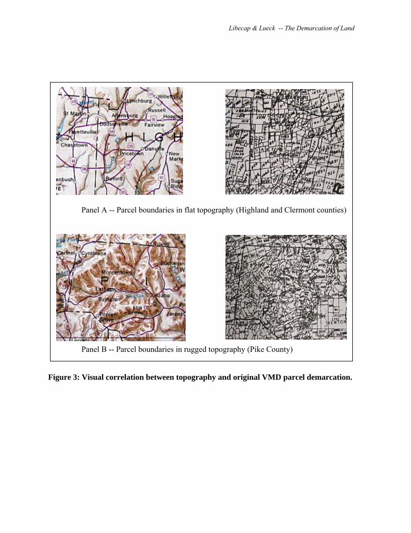
Libecap & Lueck -- The Demarcation of Land
Panel A -- Parcel boundaries in flat topography (Highland and Clermont counties)
Panel B -- Parcel boundaries in rugged topography (Pike County)
Figure 3: Visual correlation between topography and original VMD parcel demarcation.
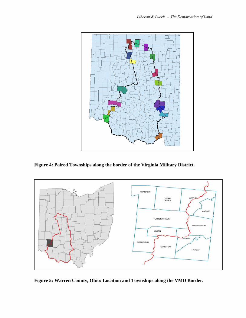
Libecap & Lueck -- The Demarcation of Land
Figure 4: Paired Townships along the border of the Virginia Military District.
` Figure 5: Warren County, Ohio: Location and Townships along the VMD Border.

Libecap & Lueck -- The Demarcation of Land
Table 1—COMPARISON OF METES AND BOUNDS AND US RECTANGULAR SYSTEMS FEATURE Metes & Bounds Rectangular Survey
Legal institutions State, common law Federal law Parcel shape Varies, idiosyncratic Square (sections) – linked to chains, acres Parcel description Perimeter – natural features Township location system Survey before claim No Yes Alignment None North-South Information Local Nationwide system

Libecap & Lueck -- The Demarcation of Land
Table 2 -- A COMPARISON OF VMD AND ADJACENT COUNTIES
CHARACTERISTIC VMD region
VMD
Counties
Surrounding
Counties
VMD value as % of Surrounding
County Value Number of Counties 39 13 26 ----
Number of Townships 437 139 298 ---- Average size of counties (miles2) 468 488 458 107 LAND CHARACTERISTICS
Soil Quality (percent prime farmland) 24.5 26.8 23.3 115 Terrain Ruggedness (0 = flat, 1 = vertical) .033 .031 .034 91 Stream Density (miles/√miles) 12.30 11.4 12.7 89 DEMOGRAPHIC CHARACTERISTICS
Average Age of Land Owner (years) 44 44 44 100 Farmers (%) 94 94 94 100 Born in Ohio (%) 37 44 34 129 Born in Virginia (%) 17 23 18 127 Notes: Averages are reported for county size and natural characteristics. A two-sample t-test between the groups was performed for each natural feature. In each case the mean value from the VMD counties was not statistically different from the mean value from the surrounding counties at the 5% level (Soil Quality: t = .81, df = 37, P = .23; Terrain Ruggedness: t = -.32, df = 37, P = .75; Stream Density: t = -.96, df = 37, P = .34; Average Age: t = -.03, df = 37; Percent Farmer: t = .06, df = 37; Percent Virginian: t = 1.76, df = 37.) The demographic variables are drawn from the 1850 and 1860 population census schedules.
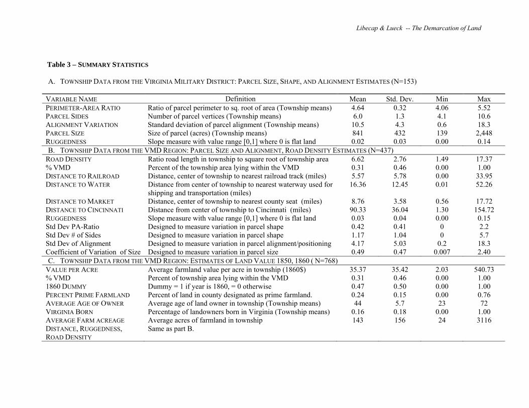
Libecap & Lueck -- The Demarcation of Land
Table 3 – SUMMARY STATISTICS A. TOWNSHIP DATA FROM THE VIRGINIA MILITARY DISTRICT: PARCEL SIZE, SHAPE, AND ALIGNMENT ESTIMATES (N=153)
VARIABLE NAME Definition Mean Std. Dev. Min Max PERIMETER-AREA RATIO Ratio of parcel perimeter to sq. root of area (Township means) 4.64 0.32 4.06 5.52 PARCEL SIDES Number of parcel vertices (Township means) 6.0 1.3 4.1 10.6 ALIGNMENT VARIATION Standard deviation of parcel alignment (Township means) 10.5 4.3 0.6 18.3 PARCEL SIZE Size of parcel (acres) (Township means) 841 432 139 2,448 RUGGEDNESS Slope measure with value range [0,1] where 0 is flat land 0.02 0.03 0.00 0.14 B. TOWNSHIP DATA FROM THE VMD REGION: PARCEL SIZE AND ALIGNMENT, ROAD DENSITY ESTIMATES (N=437)
ROAD DENSITY Ratio road length in township to square root of township area 6.62 2.76 1.49 17.37 % VMD Percent of the township area lying within the VMD 0.31 0.46 0.00 1.00 DISTANCE TO RAILROAD Distance, center of township to nearest railroad track (miles) 5.57 5.78 0.00 33.95 DISTANCE TO WATER
Distance from center of township to nearest waterway used for shipping and transportation (miles)
16.36 12.45 0.01 52.26
DISTANCE TO MARKET Distance, center of township to nearest county seat (miles) 8.76 3.58 0.56 17.72 DISTANCE TO CINCINNATI Distance from center of township to Cincinnati (miles) 90.33 36.04 1.30 154.72 RUGGEDNESS Slope measure with value range [0,1] where 0 is flat land 0.03 0.04 0.00 0.15 Std Dev PA-Ratio Designed to measure variation in parcel shape 0.42 0.41 0 2.2 Std Dev # of Sides Designed to measure variation in parcel shape 1.17 1.04 0 5.7 Std Dev of Alignment Designed to measure variation in parcel alignment/positioning 4.17 5.03 0.2 18.3 Coefficient of Variation of Size Designed to measure variation in parcel size 0.49 0.47 0.007 2.40 C. TOWNSHIP DATA FROM THE VMD REGION: ESTIMATES OF LAND VALUE 1850, 1860 ( N=768)
VALUE PER ACRE Average farmland value per acre in township (1860$) 35.37 35.42 2.03 540.73 % VMD Percent of township area lying within the VMD 0.31 0.46 0.00 1.00 1860 DUMMY Dummy = 1 if year is 1860, = 0 otherwise 0.47 0.50 0.00 1.00 PERCENT PRIME FARMLAND Percent of land in county designated as prime farmland. 0.24 0.15 0.00 0.76 AVERAGE AGE OF OWNER Average age of land owner in township (Township means) 44 5.7 23 72 VIRGINIA BORN Percentage of landowners born in Virginia (Township means) 0.16 0.18 0.00 1.00 AVERAGE FARM ACREAGE Average acres of farmland in township 143 156 24 3116 DISTANCE, RUGGEDNESS, ROAD DENSITY
Same as part B.

Libecap & Lueck -- The Demarcation of Land
D. COUNTY DATA FOR THE VMD REGION (1858, 1859): ESTIMATES OF MARKET TRANSACTIONS (N=39)
E. FARM DATA FROM WARREN COUNTY (1868, 1870): ESTIMATES OF LAND VALUES (N=456) VALUE PER ACRE Value of farm divided by farm acreage 89.36 61.68 12.43 766.36 VMD Dummy = 1 if farm location is in VMD; = 0 otherwise 0.42 0.49 0.00 1.00 PERCENT PRIME FARMLAND Percent of farm in Land Capability Class of prime farmland 0.51 0.19 0.03 0.96 DISTANCE TO ROAD Distance from center of farm to the nearest road 0.17 0.07 0.07 0.56 DISTANCE TO RAILROAD Distance from center of farm to the nearest railroad track 2.21 1.77 0.07 6.57 DISTANCE TO WATER Distance from center of farm to the nearest waterway used for
shipping and transportation 4.99 3.11 0.05 14.20
DISTANCE TO MARKET Distance from center of farm to the county seat, Lebanon, Oh 8.88 2.94 1.63 14.99 STREAM DENSITY miles/√miles in a township 3.63 4.92 0 33.32 RUGGEDNESS Township slope measure, value range [0,1] where 0 is flat land 0.03 0.01 0.00 0.09 AGE OF OWNER Age of landowner in years 51 13 14 85 FARM ACREAGE Total acres of farm 123 78.5 3 526
Sources: See Data Appendix
MORTGAGES Number of farm mortgages recorded (1858, 1859 mean) 678 394 160 2280 CONVEYANCES Number of property conveyances (1858-1859 mean) 288 232 39 1228 % VMD Percent of county area lying within the VMD 0.35 0.40 0.00 1.00 POPULATION Population of county in 1860 29,184 32,072 13,015 216,410 NUMBER OF FARMS Total number of farms in county 1860 1925 588 1045 3520 TOTAL FARM ACREAGE Total acreage of farmland in county 1860 242,017 52,002 140,352 388,823 FARM VALUE PER ACRE Average value per acre in county 1860 34.59 16.28 13.57 98.47 RUGGEDNESS Slope measure with value range [0,1] where 0 is flat land 0.03 0.03 0.01 0.12

Libecap &Lueck – The Demarcation of Land
Table 4 -- ESTIMATES OF PARCEL SHAPE (VMD TOWNSHIPS ONLY)
INDEPENDENT VARIABLES
(1) (2) (3) (4) Perimeter-Area
Ratio Number of
Sides Std. Dev of Alignment Parcel Size
RUGGEDNESS 6.219*** 25.45*** 31.06*** -4060*** [0.537] [2.114] [7.227] [695.4] CONSTANT 4.572*** 5.638*** 10.20*** 732.5*** [0.0285] [0.112] [0.383] [36.87] Observations (townships) 153 153 153 153 R2 0.471 0.490 0.109 0.184 F-Statistic 134.3 144.9 18.47 34.09 Notes: Results are reported from weighted regression models of parcel shape characteristics. The dependent variables are labeled at the top of each column. The parameter estimates for the independent variables are reported with their standard errors listed below in brackets (*** p<0.01, ** p<0.05, * p<0.1). Observations were weighted by the number of parcels in a township. When using standard errors that are corrected for spatial dependence (not reported) significance levels of the independent variables do not change.

Libecap & Lueck -- The Demarcation of Land
Table 5 -- ESTIMATES OF VARIATION IN PARCEL SHAPE, SIZE, AND ALIGNMENT (VMD AND ADJACENT TOWNSHIPS)
INDEPENDENT VARIABLES
(1) (2) (3) (4) Std. Dev.
Perimeter-Area Ratio
Std. Dev. Number of Sides
Std. Dev. of Alignment
Coeff. of Var. Parcel Size
% VMD 0.456*** 1.757*** 9.022*** 0.334*** [0.0511] [0.0930] [0.365] [0.0689] RUGGEDNESS -0.343 0.739 9.049** -0.100 [0.527] [0.959] [3.761] [0.711] INTERACTION 3.577*** 7.952*** 23.76*** 7.041*** [0.867] [1.578] [6.189] [1.169] CONSTANT 0.331*** 0.615*** 0.926*** 0.470*** [0.0263] [0.0479] [0.188] [0.0355] Observations (townships) 437 437 437 437 R2 0.401 0.702 0.777 0.335 F-Statistic 96.0 337.1 498.1 72.2 Notes: Results are reported from weighted regression models of parcel shape characteristics. The dependent variables are labeled at the top of each column. The parameter estimates for the independent variables are reported with their standard errors listed below in brackets (*** p<0.01, ** p<0.05, * p<0.1). Observations are weighted by the number of parcels in a township.
Table 6-- 19TH CENTURY OHIO SUPREME COURT PROPERTY DISPUTE RATES Disputes (per 1,000 parcels)
VMD metes & bounds
non-VMD rectangular system
Ratio of dispute rates: MB/RS
Boundary
1.46 0.37 3.95
Validity of Entry/patent
8.61 0.26 33.12
Validity of Survey
2.48 0.08 31.00
TOTAL 12.54 0.71 17.66 Notes: The Ohio Supreme Court data is normalized by dividing by the total number of parcels corresponding to each group and multiplying by 1,000. Parcel source data comes from the geospatial dataset Ohio Original Land Subdivisions (McDonald et al, Ohio Division of Geological Survey, Columbus, OH, 2002). Total number of parcels in VMD = 6,856 and Non-VMD = 61,688.

Libecap & Lueck -- The Demarcation of Land
Table 7 -- ESTIMATES OF LAND TRANSACTIONS IN VMD REGION (1860) INDEPENDENT Mortgages Conveyances
VARIABLES Total Per Acre Per 1,000
People Total Per Acre Per 1,000
People %VMD -0.0862 -0.204 -0.117 -0.486*** -0.527*** -0.489*** [0.125] [0.121] [0.130] [0.173] [0.159] [0.155] SOIL QUALITY 0.871* 0.823* 0.206 0.633 0.930 -0.0768 [0.458] [0.422] [0.477] [0.631] [0.553] [0.569] RUGGEDNESS -3.093* -4.815*** -5.005*** -6.485*** -7.678*** -7.917*** [1.636] [1.673] [1.684] [2.254] [2.193] [2.005] POPULATION/1000 0.00407** 0.0061*** -- 0.00757*** 0.00862*** -- [0.00197] [0.00195] -- [0.00272] [0.00255] -- FARMS/1000 0.533*** 0.333*** -0.0787 0.344 0.297* -0.0853 [0.148] [0.118] [0.111] [0.204] [0.154] [0.132] FARM ACRES/1000 -0.000410 -- 0.000681 0.00199 -- 0.00221 [0.00150] -- [0.00148] [0.00206] -- [0.00176] CONSTANT 5.247*** -0.0911 3.334*** 4.282*** -0.866*** 2.316*** [0.247] [0.226] [0.256] [0.340] [0.296] [0.305] Observations (counties) 39 39 39 39 39 39 R-squared 0.76 0.72 0.28 0.73 0.72 0.46 F Statistic 16.77 17.27 2.54 14.12 17.11 5.64 Notes: Results are reported from regression models of market transactions. The parameter estimates for the independent variables are reported with their standard errors listed below in brackets (*** p<0.01, ** p<0.05, * p<0.1). When using standard errors that are corrected for spatial dependence (not reported) significance levels of the independent variables do not change.

Libecap & Lueck -- The Demarcation of Land
Table 8 - Pair-wise Comparison of Mean Township Per-Acre Land Values Non-VMD VMD
Mean $36.14 $31.69 Standard Deviation $16.56 $12.30 Observations 26 26 T-statistic (P-value, 1-tail) 1.88 (0.036)
Table 9 -- WARREN COUNTY SAMPLE - COMPARISON OF MB AND RS FARMS
Characteristics RS farms MB farms AREA (miles2) 234 173 NUMBER OF FARMS 265 191
Land Characteristics SOIL QUALITY (% prime farmland) 60 38 RUGGEDNESS (0 = flat, 1 = vertical) 0.025 0.025 STREAM DENSITY (miles/√miles) 1.44 6.67 Land Characteristics AVERAGE AGE OF LAND OWNER (years) 51 50 Notes: Sample mean values are reported with standard deviations in brackets. A two-sample t-test between groups was performed on the variables with the exception of the Farmer Dummy Variable in which Fisher’s exact test was used. (Soil Quality: t = 14.9, df = 454, P = .000; Ruggedness: t = .33, df = 454, P = .74; Stream Density: t = -13.14, df = 454, P = .000; Age: t = 1.01, df = 454)

Libecap & Lueck -- The Demarcation of Land
Table 10 – ESTIMATES OF PER-ACRE FARMLAND VALUE IN WARREN COUNTY, OHIO ($1870) INDEPENDENT VARIABLES 1 2 3 4 VMD (dummy for MB) -0.14** -0.16** -0.17** -0.18** [0.072] [0.073] [0.074] [0.076] % PRIME FARMLAND 0.90*** 0.90*** 0.90*** 0.90*** [0.15] [0.15] [0.15] [0.15] RUGGEDNESS -4.05* -4.44* -3.79 -4.18* [2.34] [2.38] [2.49] [2.53] STREAM DENSITY -0.062*** -0.050*** -0.054*** -0.042** [0.018] [0.017] [0.019] [0.018] DISTANCE TO RIVER 0.037*** 0.036*** 0.033*** 0.032*** [0.0092] [0.0093] [0.0092] [0.0093] FARM ACREAGE -0.0011*** -0.0011*** [0.00031] [0.00031] ROAD DENSITY 0.048*** 0.048** [0.018] [0.019] DISTANCE TO RAILROAD -0.042** -0.028 -0.032 -0.019 [0.020] [0.019] [0.020] [0.019] DISTANCE TO MARKET -0.018 -0.022* -0.015 -0.018 [0.011] [0.011] [0.012] [0.012] DISTANCE TO CINCINNATI -0.0056 -0.0093 -0.0062 -0.0099 [0.0061] [0.0061] [0.0063] [0.0063] AGE 0.0029 0.0020 0.0017 0.00080 [0.0096] [0.0096] [0.0099] [0.0099] AGE2 -0.000025 -0.000014 -0.000020 -8.8e-06 [0.000093] [0.000093] [0.000096] [0.000096] CONSTANT 3.98*** 4.61*** 3.84*** 4.46*** [0.36] [0.30] [0.37] [0.31] Observations (farms) 456 456 456 456 Adjusted R-squared 0.29 0.28 0.268 0.259 F Statistic 26.0 28.1 26.8 29.4 Notes: Results are reported from regression models of land value. The parameter estimates for the independent variables are reported with robust standard errors in brackets (*** p<0.01, ** p<0.05, * p<0.1).

Libecap & Lueck -- The Demarcation of Land
Table 11– ESTIMATES OF LAND VALUE PER ACRE (1860$)
INDEPENDENT VARIABLES (1)
(2)
(3) (4) %VMD -0.24*** -0.26*** -0.25*** -0.28*** [0.060] [0.061] [0.065] [0.065] RUGGEDNESS -3.62*** -3.80*** -3.72*** -3.91*** [0.73] [0.73] [0.73] [0.72] %VMD*RUGGEDNESS 4.77*** 4.90*** 4.84*** 4.98*** [1.43] [1.46] [1.43] [1.46] 1860 DUMMY 0.53*** 0.53*** 0.53*** 0.53*** [0.023] [0.023] [0.023] [0.023] % PRIME FARMLAND 0.40** 0.43** 0.38** 0.40** [0.19] [0.18] [0.19] [0.19] AVERAGE FARM SIZE -0.00037* -0.00037* [0.00020] [0.00019] ROAD DENSITY 0.017** 0.017** [0.0080] [0.0081] DISTANCE TO RAILROAD -0.026*** -0.027*** -0.026*** -0.027*** [0.0039] [0.0039] [0.0039] [0.0040] DISTANCE TO RIVER -0.0071*** -0.0077*** -0.0073*** -0.0079*** [0.0016] [0.0016] [0.0016] [0.0016] DISTANCE TO MARKET -0.015** -0.015** -0.015** -0.016** [0.0058] [0.0059] [0.0060] [0.0060] DISTANCE TO CINCINNATI -0.0070*** -0.0075*** -0.0069*** -0.0075*** [0.00098] [0.00098] [0.00099] [0.00100] AGE 0.051* 0.051* 0.052* 0.052* [0.029] [0.029] [0.029] [0.029] AGE2 -0.00051 -0.00052 -0.00051 -0.00052 [0.00032] [0.00032] [0.00032] [0.00032] CONSTANT 2.74*** 2.91*** 2.68*** 2.85*** [0.68] [0.69] [0.68] [0.68]
Observations (townships) 774 774 774 774 Adjusted R-squared 0.550 0.547 0.541 0.538 F Statistic 91.1 97.0 101 108 Notes: Results are from weighted regression models in which the dependent variable is the natural logarithm of average land value per acres from 1850 and 1860. Land values are in $1860. The parameter estimates for the independent variables are reported with their standard errors, clustered at the township-level, listed below in brackets (*** p<0.01, ** p<0.05, * p<0.1). Observations were weighted by percent farmland in the corresponding county.

Libecap & Lueck -- The Demarcation of Land
Table 12 – ESTIMATES OF ROAD DENSITY INDEPENDENT VARIABLES
Roads VMD % -0.243*** [0.0478] DISTANCE TO RAILROAD -0.00720* [0.00394] DISTANCE TO RIVER -0.00454** [0.00184] DISTANCE TO MARKET -0.00264 [0.00529] DISTANCE TO CINCINNATI -0.00507*** [0.000532] RUGGEDNESS -2.722*** [0.588] CONSTANT 2.559*** [0.0589] Observations (townships) 437 F Statistic 36.66 R-squared 0.261 Notes: Results are reported from regression models in which the dependent variable is the natural log of road density in a township. The dependent variables are labeled at the top of each column. The parameter estimates for the independent variables are reported with their standard errors listed below in brackets (*** p<0.01, ** p<0.05, * p<0.1). When using standard errors that are corrected for spatial dependence (not reported) significance levels of the independent variables do not change.

Libecap & Lueck -- The Demarcation of Land
Data Appendix CONSTRUCTED VARIABLES Geographical Polygon Features (counties, townships, parcels, VMD)
Geographical boundaries for Ohio counties, townships, parcels, and the Virginia Military District were obtained from the digital map Original Land Subdivisions of Ohio (Ohio Department of Natural Resources, 2006). The map represents the digital compilation of the original land subdivisions in Ohio, styled after Sherman’s (1922) map. Each unit in the map is represented by a distinct polygon in the spatial dataset. All polygon measures of area, perimeter, and centroid location used in the analysis are calculated from this dataset using geographical information systems (GIS) software. The “original” land subdivisions likely represent very early ownership patterns. They do not appear to have been the first sales of federal or Virginia land to private claimants. Some of those transactions were very large and no parcel is of that size. Land speculation and subdivision was common throughout the Ohio frontier, and these parcels were subdivided as census data on farm sizes reveal. Farms were much smaller still. The mean of parcel size in the RS was 637 acres with SD 113; for the VMD the mean was 813 with a SD of 611. Farm Size (acres): (1850) MB – mean = 173, sd = 235; RS – mean = 130, sd = 59. (1860) MB – mean = 157, sd = 235; RS – mean = 130, sd = 59 (parcels from Sherman and farm sizes from the 1850 and 1860 census sample). Perimeter-Area Ratio of Parcel
Using the Original land subdivisions of Ohio dataset, we relate the perimeter of a parcel’s boundary to the parcel’s area with the metric:
√
Number of Parcel Sides To calculate this metric we intentionally modified our source data of parcel boundaries to
make meaningful counts of polygon vertices. Polygons in our parcel dataset contain many vertices that are an artifact of the digitization process. To correct for this, the polygon shape file is modified using a simple algorithm based on a method developed by Douglas and Peucker (1973) to remove redundant points, such as over-digitized vertices.∗ The remaining sample represents the unique vertices of the original polygons. Counting them gives the value for the variable NUMBER OF PARCEL SIDES. Parcel Alignment
We define alignment by the angle θ of the longest side of a parcel where θ is measured from a true North-South baseline. The orientation angle θ is measured in decimal degrees and has the range [-90, 90]. When coordinating rectangles in a grid, a value of θ and its right angle counterparts will all represent the same alignment of the parcel. For example, the measurements θ = -90, θ = 0, and θ = 90, are all consistent with an alignment based on true north. To equate values which represent the same alignment we use ALIGNMENT min |0 |, 90 | | which has the range [0, 45]. For more information, contact the authors. Ruggedness
From the USGS National Elevation Dataset we calculate the slope of the area covered by the digital elevation models, DEM. The slope of a given cell in the DEM is calculated using the change in elevation from its eight neighboring cells. From this the rate of change in elevation is calculated and then used to develop a slope measure with a range of [0, 90], where 0 represents flat land. Terrain ruggedness is then calculated as slope/90 with a possible range of [0,1]. When used
∗ Technical paper, ESRI Inc., "Automation of Map Generalization: The Cutting-Edge Technology", 1996. It can be found in the White Papers section of ArcOnline at this Internet address: http://downloads.esri.com/support/whitepapers/ao_/mapgen.pdf
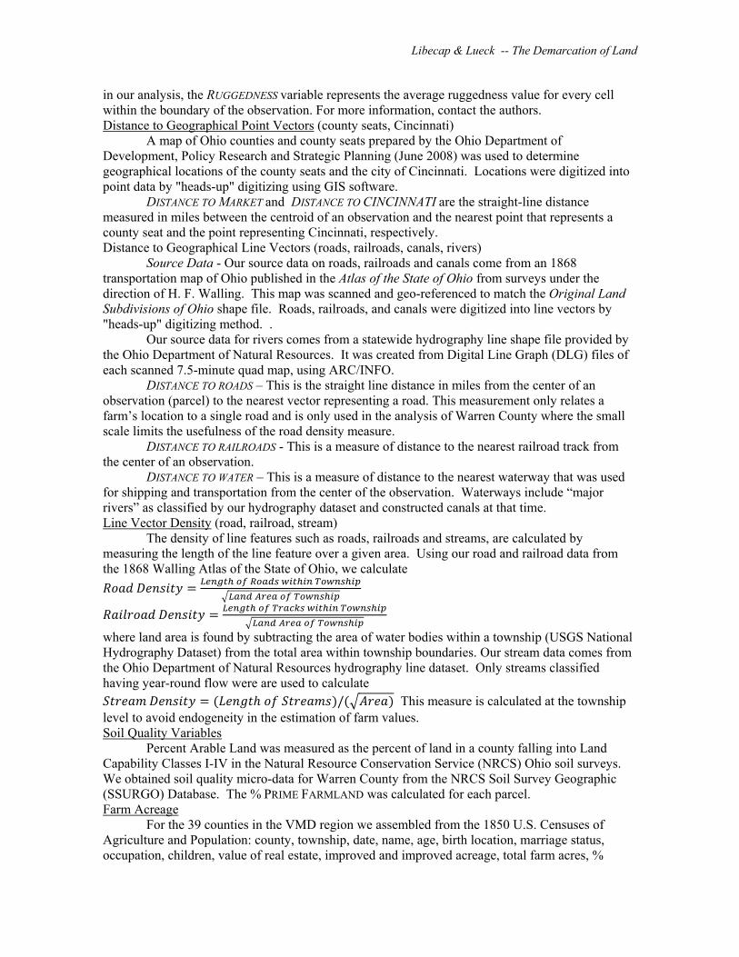
Libecap & Lueck -- The Demarcation of Land
in our analysis, the RUGGEDNESS variable represents the average ruggedness value for every cell within the boundary of the observation. For more information, contact the authors. Distance to Geographical Point Vectors (county seats, Cincinnati)
A map of Ohio counties and county seats prepared by the Ohio Department of Development, Policy Research and Strategic Planning (June 2008) was used to determine geographical locations of the county seats and the city of Cincinnati. Locations were digitized into point data by "heads-up" digitizing using GIS software.
DISTANCE TO MARKET and DISTANCE TO CINCINNATI are the straight-line distance measured in miles between the centroid of an observation and the nearest point that represents a county seat and the point representing Cincinnati, respectively. Distance to Geographical Line Vectors (roads, railroads, canals, rivers)
Source Data - Our source data on roads, railroads and canals come from an 1868 transportation map of Ohio published in the Atlas of the State of Ohio from surveys under the direction of H. F. Walling. This map was scanned and geo-referenced to match the Original Land Subdivisions of Ohio shape file. Roads, railroads, and canals were digitized into line vectors by "heads-up" digitizing method. .
Our source data for rivers comes from a statewide hydrography line shape file provided by the Ohio Department of Natural Resources. It was created from Digital Line Graph (DLG) files of each scanned 7.5-minute quad map, using ARC/INFO.
DISTANCE TO ROADS – This is the straight line distance in miles from the center of an observation (parcel) to the nearest vector representing a road. This measurement only relates a farm’s location to a single road and is only used in the analysis of Warren County where the small scale limits the usefulness of the road density measure. DISTANCE TO RAILROADS - This is a measure of distance to the nearest railroad track from the center of an observation.
DISTANCE TO WATER – This is a measure of distance to the nearest waterway that was used for shipping and transportation from the center of the observation. Waterways include “major rivers” as classified by our hydrography dataset and constructed canals at that time. Line Vector Density (road, railroad, stream)
The density of line features such as roads, railroads and streams, are calculated by measuring the length of the line feature over a given area. Using our road and railroad data from the 1868 Walling Atlas of the State of Ohio, we calculate
where land area is found by subtracting the area of water bodies within a township (USGS National Hydrography Dataset) from the total area within township boundaries. Our stream data comes from the Ohio Department of Natural Resources hydrography line dataset. Only streams classified having year-round flow were are used to calculate
/ This measure is calculated at the township level to avoid endogeneity in the estimation of farm values. Soil Quality Variables
Percent Arable Land was measured as the percent of land in a county falling into Land Capability Classes I-IV in the Natural Resource Conservation Service (NRCS) Ohio soil surveys. We obtained soil quality micro-data for Warren County from the NRCS Soil Survey Geographic (SSURGO) Database. The % PRIME FARMLAND was calculated for each parcel. Farm Acreage
For the 39 counties in the VMD region we assembled from the 1850 U.S. Censuses of Agriculture and Population: county, township, date, name, age, birth location, marriage status, occupation, children, value of real estate, improved and improved acreage, total farm acres, %

Libecap & Lueck -- The Demarcation of Land
improved, farm land value, farm land value per acre, number of livestock, livestock value, total farm value, total farm value per acre, crops, and value of slaughtered animals. From the 1860 U.S. Censuses, we assembled the same variables, calculating farm size. Farm Value
The U.S. Census of Agriculture reports farmland value that includes the value of land and buildings as well as total farm value that includes the value of livestock and implements. In the paper we report estimates using the farmland value, although we have also estimated our specification using total farm value and found similar results.
PAIRED TOWNSHIP TESTS Selecting Pairs: The sample of paired townships was created following these steps.
1. Townships were selected that bordered the VMD. 2. A township with more than 80% of its area within the VMD was identified as a MB
township, and a township with more than 80% of its area outside of the VMD was identified as a RS township. If we use only pairs of townships where one is completely within the VMD and the other is completely outside the VMD, we would only get a sample size of 6 pairs.
3. If a MB and RS township shared a boundary at any point, they were considered a potential pair.
4. Potential pairs were then matched to the available summary data on townships from the 1850 and 1860 Agricultural Census (‘farm townships’ tab in the master dataset). Data from 1850 and 1860. Pairs were only kept in the sample if both townships were represented in the same census.
Several townships were paired with more than one township. The final pairs were selected by maximizing the total length of shared boundaries in the sample with the constraint that each township could only be represented in one pair. Farm value data were converted to 1860 prices. Mean land values were compared both with the full sample and with dropping two outliers outside and within the VMD that had much higher land values would have biased the test in favor of finding higher values outside the VMD. Data Sampling VMD and Adjacent Counties.
The 39 counties included in the analysis are listed with (% in VMD) Adams (100), Allen (0), Auglaize (0), Brown (100), Butler (0), Champaign (32), Clark (18), Clermont (100), Clinton (100), Crawford (0), Delaware (.14), Fairfield (0), Fayette (100), Franklin (40), Greene (67), Hamilton (9), Hancock (0), Hardin (41), Highland (100), Hocking (0), Jackson (0), Knox (0), Lawrence (0), Licking (0), Logan (58), Madison (100), Marion (15), Miami (0), Montgomery (0), Morrow (0), Pickaway (57), Pike (64), Ross (70), Scioto (48), Shelby (0), Union (100), Vinton (0), Warren (42), and Wyandot (0). Township Level Analysis.
Ohio data from the 1850 and 1860 Censuses of Agriculture and Population, were entered into excel from microfilm copies of the original schedules. The population schedules were obtained from Ancestry.com and Geneology.com and the agriculture schedules from the National Archives. Both census years were sampled to secure a sample of sufficient size for analysis. We were not able to match census entries with the original parcel maps, which apparently is a common problem. Counties partially or completely in the VMD, as well as counties adjacent to the district, were sampled. For 1850, these included Adams, Allen, Auglaize, Brown, Butler, Delaware, Fairfield, Franklin, Fayette, Greene, Hamilton, Hancock, Hardin, Highland, Hocking, Knox, Lawrence, Licking, Logan, Madison, Marion, Miami, Montgomery, Ross, Scioto, Shelby, Union, Vinton, Warren, and Wyandot. For 1860 the same counties were sampled, except for Miami, Shelby, Union, Vinton, Warren, and Wyandot, which were unavailable because these original surveys were destroyed prior to microfilming. In the analysis individual observations are averaged by township.

Libecap & Lueck -- The Demarcation of Land
Because of the lost county data for 1860, we have 768 township observations, rather than potentially 874 (437 townships in the VMD and adjacent counties x 2). The 1850 census was sampled at approximately a 10 percent rate, but a 5 percent rate was used for the more comprehensive 1860 census. Data from the Census of Agriculture were matched to the farmer’s population census records for the corresponding years. The matches were made using a searchable electronic database available by description at Ancestry.com. For both census periods, we were able to match an average of over 60 percent of the farms. Warren County Analysis.
1867 Parcel maps of farms in Warren County, Ohio (split by the VMD) were obtained from http://www.rootsweb.ancestry.com/~ohwarren/maps/1867map.htm. "Map of Warren Co Ohio from actual Surveys by G. P. Sanford, J. Silliman Higgins & R. H. Harrison, Civil Engineers; A. Warner Publisher; Philadelphia, 1867." Names from the 1867 plat map were matched to names from the 1870 population census via Ancestry.com. These names were then matched to farmer names on the 1870 agricultural census schedule on microfilm (National Archives, Non Population Census Records: Ohio, 1870, T1159, Role 42. We recorded the value of land and buildings and total value of farms (value of land and buildings, value of livestock, value of implements and machinery). County Level Analysis
Annual conveyance and mortgage data are from Second Annual Report of the Commissioner of Statistics, to the General Assembly of Ohio: For the Fiscal Year 1858. Columbus, Ohio: Richard Nevins, State Printer. 1859 and the Third Annual Report of the Commissioner of Statistics, to the General Assembly of Ohio: For the Fiscal Year 1859 Columbus, Ohio: Richard Nevins, State Printer. 1860. The mean value for the two years is used in the regressions. 1860 was not available to us. Population and county size are from 1860 Census, Geospatial & Statistical Data Center; see http://fisher.lib.virginia.edu/collections/stats/histcensus/php/county.php .
OHIO COURT ANALYSIS
We searched compendiums of Ohio court cases in the 19th century and then turned to Westlaw and Lexis/Nexis for case reports: Page’s Ohio Digest: A Digest of All Reported Decisions of the Courts of Ohio from the Earliest Period to Date, John L. Mason Editor in Chief, Volume One, Part One, Abandonment to Assault and Battery; Part Two, Assignments to Charities, Volume Four, Deeds to Equity, Volume Eight, Subrogation to Youthful Employee, Cincinnati: The W.H. Anderson Company, 1914; A Digest of All Reported Decisions of the Courts of Ohio from the Earliest Period to Date, Lifetime Edition, edited by William Herbert Page, Volume 10, Parties to Receipts, Volume Twelve, Part One, Taxation to Venditioni Exponas, Cincinnati: W.H. Anderson Company, 1936. Ohio Jurisprudence: A Complete Statement of the Law and Practice of the State of Ohio with Forms, Editor in Chief: Willis A. Estrich, Consulting Editor William M. McKinney, Managing Editor, George S. Gulick, Volume 1, 1928, Historical Introduction to Adverse Possession; Volume 5, Bail to Boundaries, 1929, Volume 15, 1931, Easements to Encumbrance, Volume 32, 1934; Pledges to Public Schools, Volume 39, 1935, Taxpayers’ Actions to Trial, Rochester, New York: The Lawyers Co-operative Publishing Company. The Lexis/Nexis search used terms: boundary, quiet title, trespass, and ejectment. Survey Validity Issues:
These cases involve a dispute where two different surveys claim the same land, for example, McArthur v. Phoebus, 2 Ohio 415 (1826). In these, the general question is which survey was valid and which was invalid. This should be differentiated from cases where two parties claim the same land because the survey, or several competing surveys, does not clearly delineate a line between the properties. These cases generally hinge on whether the survey was correctly recorded or implemented. In general, these cases are more common in VMD areas, but do exist in RS areas of Ohio, but the issues are far easier to resolve in the latter, generally hinging on resolving a clear surveying error, rather than conflicting land claims. See Hamil v. Carr, 21 O.S. 258 (Ohio 1871).

Libecap & Lueck -- The Demarcation of Land
Boundary Issues: This is a broader area of conflict, and includes cases where there is a dispute about where a
boundary line actually stands. The majority of relevant cases fall in this area and typically occur because the survey, or multiple surveys, do not make it legally clear where the boundary line stands. These cases also frequently occur when a deed does not make clear part of a plat it is granting. oth these disputes occur in VMD and non-VMD areas, although the former are generally far more omplex, hinge on far less clear legal principles, and occur with greater frequency than in RS (non-VMD) area Validity of Deeds/Patents:
These cases occur frequently and all hinge on whether a deed or patent was valid. While these are actually two fairly different legal issues, they generally depend on the same type of questions, namely was the deed/patent correctly recorded under the relevant statute and does the deed/patent correctly describe the land it grants. If not, the deed/patent is generally invalid. For the most part, these cases do not involve any boundary disputes, except in the cases where the validity of a patent is used as a collateral attack on cases of overlapping surveys. It is worth noting, however, that patent validity seems to be an issue mostly in VMD cases, largely due to the complexity of the issues involved. The case, Ohio (Pt 1) 206 Porter v Robb from Clermont County illustrates some of the boundary problems found in the VMD, especially where there was a chain of entries and surveys. See also Huston v McArthur, 7 O (Pt 2) 54.
NET PRESENT VALUE CALCULATIONS To determine survey costs, we counted the number of townships or parts of townships in the counties adjacent to the VMD that are part of our 39 county study area. There was no double counting of township borders. All township lines are 6 miles. A township has 4, 6-mile boundary lines, 10, 6-mile internal section lines, and 16 6-mile internal half section lines. $3/mile is used as the survey cost as described in the text. We break down total survey distance into three categories: 1) borders that are both county and township lines; 2) township borders within a county; and 3) section and half-section lines within townships. We used ArcGIS and the spatial dataset cited in the paper to measure county borders and specify when the border was shared with another one of the 39 counties in the sample. We put the cost of shared borders on the county that would have been surveyed first assuming surveyors started in the north east corner of the sample and traveled outward (south and west). The total length of township borders within a county was also calculated using ArcGIS and the spatial dataset. (We made sure that these distances did not include county borders). Lastly, using the total number of non-VMD townships in each county, we add 60 miles of surveying per township for our estimate of costs using sections, and 96 miles of surveying per township for our estimate of townships with half-sections. The total mileage is multiplied by $3 for total cost. Total cost is divided by total non-VMD farm acreage ([1-%VMD]*farmland) to get survey cost per acre of farmland. Survey costs were $82,081 if sections were surveyed and $122,689 if half sections were surveyed. The RS counties had 5,950,774 acres of farm land in 1860, calculated from the 1860 agricultural census, meaning that average survey costs were $.0138 or $.0206/ acre.