Systems of interacting diffusions with partial annihilationthrough membranes ∗

Zhen-Qing Chen and Wai-Tong (Louis) Fan

April 4, 2014

Abstract

We introduce an interacting particle system in which two families of reflected diffusionsinteract in a singular manner near a deterministic interface I. This system can be usedto model the transport of positive and negative charges in a solar cell or the populationdynamics of two segregated species under competition. A related interacting random walkmodel with discrete state spaces has recently been introduced and studied in [9]. In thispaper, we establish the functional law of large numbers for this new system, thereby extendingthe hydrodynamic limit in [9] to reflected diffusions in domains with mixed-type boundaryconditions, which include absorption (harvest of electric charges). We employ a new anddirect approach that avoids going through the delicate BBGKY hierarchy.

AMS 2000 Mathematics Subject Classification: Primary 60F17, 60K35; Secondary 92D15

Keywords and phrases: hydrodynamic limit, interacting diffusion, reflected diffusion, anni-hilation, non-linear boundary condition, coupled partial differential equation, martingales

1 Introduction

With motivation to model and analyze the transport of positive and negative charges in solarcells, an interacting random walk model in domains has recently been introduced in [9]. In thatmodel, a bounded domain in Rd is divided into two adjacent sub-domains D+ and D− by aninterface I. The subdomains D+ and D− represent the hybrid medias which confine the positiveand the negative charges, respectively. At microscopic level, positive and negative charges aremodeled by independent continuous time random walks on lattices inside D+ and D−. Thesetwo types of particles annihilate each other at a certain rate when they come close to eachother near the interface I. This interaction models the annihilation, trapping, recombinationand separation phenomena of the charges. Such a stochastic system can also model populationdynamics of two segregated species under competition near their boarder. Under an appropriatescaling of the lattice size, the speed of the random walks and the annihilation rate, we provedin [9] that the hydrodynamic limit is described by a system of nonlinear heat equations that are

∗Research partially supported by NSF Grants DMR-1035196 and DMS-1206276.

1

coupled on the interface and satisfy Neumann boundary condition at the remaining part of theboundary.

While the random walk model in [9] is more amenable to computer simulation, it is subjectto technical restrictions associated with the discrete approximations of both the diffusions per-formed by the particles and the underlying domains D±. Furthermore, that model does notconsider harvest of charges.

In this paper, a new continuous state stochastic model is introduced and investigated. Thismodel is different from that of [9] in three ways: the particles perform reflected diffusions oncontinuous state spaces rather than random walks over discrete state spaces, particles are ab-sorbed (harvested) at some regions (harvest sites) away from the interface I, and the annihilationmechanism near I is different. The model in this paper allows more flexibility in modeling theunderlying spatial motions performed by the particles and in the study of their various proper-ties. In particular, it is more convenient to work with when we study the fluctuation limit (or,functional central limit theorem) of the interacting diffusion system, which is the subject of anon-going project [10].

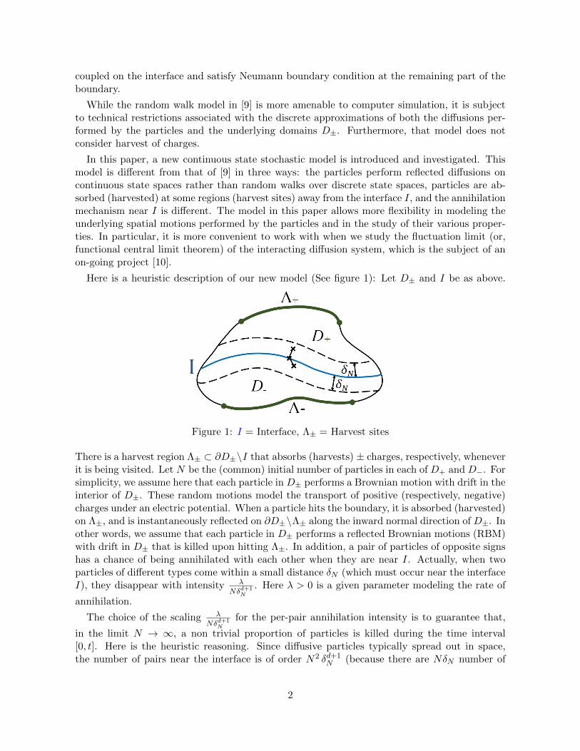
Here is a heuristic description of our new model (See figure 1): Let D± and I be as above.

Figure 1: I = Interface, Λ± = Harvest sites

There is a harvest region Λ± ⊂ ∂D±\I that absorbs (harvests) ± charges, respectively, wheneverit is being visited. Let N be the (common) initial number of particles in each of D+ and D−. Forsimplicity, we assume here that each particle in D± performs a Brownian motion with drift in theinterior of D±. These random motions model the transport of positive (respectively, negative)charges under an electric potential. When a particle hits the boundary, it is absorbed (harvested)on Λ±, and is instantaneously reflected on ∂D±\Λ± along the inward normal direction of D±. Inother words, we assume that each particle in D± performs a reflected Brownian motions (RBM)with drift in D± that is killed upon hitting Λ±. In addition, a pair of particles of opposite signshas a chance of being annihilated with each other when they are near I. Actually, when twoparticles of different types come within a small distance δN (which must occur near the interfaceI), they disappear with intensity λ

Nδd+1N

. Here λ > 0 is a given parameter modeling the rate of

annihilation.

The choice of the scaling λNδd+1

N

for the per-pair annihilation intensity is to guarantee that,

in the limit N → ∞, a non trivial proportion of particles is killed during the time interval[0, t]. Here is the heuristic reasoning. Since diffusive particles typically spread out in space,the number of pairs near the interface is of order N2 δd+1

N (because there are NδN number of

2

particles in D+ near I, and each of them is near to NδdN number of particles in D−). Withthe above choice of per-pair annihilation intensity, the expected number of pairs killed within tunits of time is about (N2 δd+1

N ) ( λNδd+1

N

t) = λNt when t > 0 is small. This implies that a non

trivial proportion of particle is annihilated during [0, t] and accounts for the boundary term inthe hydrodynamic limit.

1.1 Main result and applications

We consider the normalized empirical measures

XN,+t (dx) :=1

N

∑α:α∼t

1X+α (t)(dx) and XN,−t (dy) :=

1

N

∑β:β∼t

1X−β (t)(dy).

Here 1y(dx) stands for the Dirac measure concentrated at the point y, while α ∼ t (resp. β ∼ t)denotes the condition that particle X+

α (resp. X−β ) is alive at time t.

Our main result (Theorem 5.2) implies the following: Suppose each particle in D± is aRBM with gradient drift 1

2 ∇(log ρ±), where ρ± is a strictly positive function on D±. Sup-

pose δN tends to zero and lim infN→∞N δdN ∈ (0,∞]. If (XN,+0 , XN,−0 ) converges in distribu-

tion, then the random measures (XN,+t , XN,−t ) converge in distribution to a deterministic limit(u+(t, x)ρ+(x)dx, u−(t, y)ρ−(y)dy) for any t > 0, where (u+, u−) is the unique solution of thecoupled heat equations

∂u+

∂t=

1

2∆u+ +

1

2∇(log ρ+) · ∇u+ on (0,∞)×D+

u+ = 0 on (0,∞)× Λ+

∂u+

∂~n+=

λ

ρ+u+u− 1I on (0,∞)× ∂D+ \ Λ+

(1.1)

and ∂u−∂t

=1

2∆u− +

1

2∇(log ρ−) · ∇u− on (0,∞)×D−

u− = 0 on (0,∞)× Λ−

∂u−∂~n−

=λ

ρ−u+u− 1I on (0,∞)× ∂D− \ Λ−,

(1.2)

where ~n± is the inward unit normal vector field on ∂D± of D± and 1I is the indicator functionon I. Note that ρ± = 1 corresponds to the particular case when there is no drift.

Remark 1.1. Generalizations and Applications: Actually, Theorem 5.2 is general enough todeal with any general symmetric reflected diffusions and covers the case when the constant λis replaced by any continuous function λ(x) on I. It is routine to generalize to any continuoustime-dependent function λ(t, x) and the details are left to the readers. Moreover, it is likelythat a further generalization to tackle multiple deletion of particles near the interface (similarto that in [17]) can be done in an analogous way. As an immediate application of Theorem 5.2,we obtain an analytic formula for the asymptotic mass of positive charges harvested during thetime interval [0, T ], which is

1−∫D+

u+(T, x)ρ+(x) dx− λ∫ T

0

∫Iu+(s, z)u−(s, z) dσ(z) ds.

3

Remark 1.2. The condition lim infN→∞N δdN ∈ (0,∞] is an upper bound for the rate at whichthe annihilations distance δN tends to 0. Such kind of condition is necessary by the followingreason: The dimension of I is d + 1 lower than that of D+ × D−. So we can choose δN smallenough so that particles of different types cannot ‘see’ each other in the limit N →∞, resultinga decoupled linear system of PDEs with Dirichlet boundary condition on Λ± and Neumannboundary condition on ∂D± \ Λ±. See Example 5.3 for a rigorous statement and proof.

1.2 Key ideas

Theorem 3.2.39 of [22] from geometric theory asserts that

limδ→0

H2d(Iδ)

cd+1 δd+1= Hd−1(I), (1.3)

where Iδ := (x, y) ∈ D+ ×D− : |x − z|2 + |y − z|2 < δ2 for some z ∈ I, cd+1 is the volumeof the unit ball in Rd+1, and Hm is the m-dimensional Hausdorff measure. In Lemma 7.2, westrengthen it to

limδ→0

1

cd+1 δd+1

∫Iδf(x, y) dxdy =

∫If(z, z) dHd−1(z) (1.4)

uniformly in f from any equi-continuous family in C(D+ ×D−). Property (1.4) leads us to thefollowing key observation that

limδ→0

limN→∞

1

cd+1 δd+1E∫ T

0XN,+s ⊗ XN,−s (Iδ) ds = lim

N→∞limδ→0

1

cd+1 δd+1E∫ T

0XN,+s ⊗ XN,−s (Iδ) ds.

This interchange of limit in turn allows us to characterize the mean of any subsequential limit of(XN,+, XN,−) by comparing the integral equations (4.1) satisfied by the hydrodynamic limit withits stochastic counterpart (7.6) . Using a similar argument, we can identify the second momentof any subsequential limit, and hence characterize any subsequential limit of (XN,+, XN,−). Wepoint out here that 1

cd+1 δd+1

∫ t0 XN,+s ⊗ XN,−s (Iδ) ds quantifies the amount of interaction among

the two types of particles, and is related (but different from) the collision local time introducedin [20]. The direct approach developed in this paper to establish the hydrodynamic limit avoidsgoing through the delicate BBGKY hierarchy as was done in [9].

1.3 Literature

Interacting diffusion systems have been studied by many authors and they continue to be thesubject of active research. See [30] and [32] for such a system on a circle whose hydrodynamiclimit is established using the entropy method. We also mention [16] for a recent large deviationresult for a system of diffusions in R interacting through their ranks. This large deviationprinciple implies convergence of the system to the hydrodynamic limit. However, the methodsin these papers do not seem to work (at least not in a direct way) for our annihilating diffusionmodel due to the singular interaction on the interface.

An extensively studied class of stochastic particle systems is reaction-diffusion systems (R-Dsystems in short), whose hydrodynamic limits are described by R-D equations ∂u

∂t = 12∆u+R(u),

where R(u) is a function in u which represents the reaction. R-D systems is an important classof interacting particle systems arising from various contexts. They were investigated by many

4

authors in both the discrete setting (particles perform random walks) and the continuous setting(particles perform continuous diffusions). For instance, for the case R(u) is a polynomial in u,these systems were studied in [17, 18, 28, 29] on a cube with Neumann boundary conditions,and in [3, 4] on a periodic lattice. See also [7] for a survey of a class of discrete (lattice) modelscalled the Polynomial Model which contains the Schlogl’s model. Recently, perturbations ofthe voter models which contain the Lotka-Volterra systems are considered in [13]. The authorsshowed that the hydrodynamic limits are R-D equations and established general conditions forthe existence of non-trivial stationary measures and for extinction of the particles. Anotherstochastic particle systems which are related to our annihilation-diffusion model is the Fleming-Viot type systems ([5, 6, 24]). In [6], Burdzy and Quastel studied an annihilating-branchingsystem of two families of random walks on a domain. In their model, when a pair of parti-cles of different types meet, they annihilate each other and they are immediately reborn at asite chosen randomly from the remaining particles of the same type. So the total number ofparticles of each type remains constant over the time, and thus this Fleming-Viot type systemis different from the annihilating random walk model of [9]. The hydrodynamic limit of themodel in [6] is described by a linear heat equation with zero average temperature. An elegantresult obtained by P. Dittrich [17] is on a system of reflected Brownian motion on the unitinterval [0, 1] with multiple deletion of particles. More precisely, any k-tuples (2 ≤ k ≤ n) ofparticles with distances between them of order ε, say (xi1 , · · · , xik), disappear with intensityck(k − 1)!εk−1

∫[0,1] p(ε

2, xi1 , y) · · · p(ε2, xik , y) dy, where ck > 0 are constants and p(t, x, y) is

the transition density of the reflected Brownian motion on [0, 1]. The hydrodynamic limit is aR-D equation with reaction term R(u) = −

∑nk=2 cku

k and Neumann boundary condition. Incontrast to [17], our model has two types of particles instead of one. Moreover, the interactionof our model is singular near the boundary and gives rise to a boundary integral term in thehydrodynamic limit.

The rest of the paper is organized as follows. Preliminary materials on setup, reflecting diffu-sions, and notations are given in Section 2. A rigorous description of the interacting stochasticparticle system we are going to study in this paper is presented in Section 3. In section 4, wegive an existence and uniqueness result of solution of a coupled heat equation with non-linearboundary condition, analogous to [9, Proposition 2.19]. The full statement of our main result(Theorem 5.2) of this paper is given in section 5. Section 6 is devoted to the proof of Theorem5.2. The proof of a key proposition that identifies the first and second moments of subsequentiallimits of empirical distributions is given in Section 7.

2 Preliminaries

2.1 Reflected diffusions killed upon hitting a closed set Λ ⊂ D

Let D ⊂ Rd be a bounded Lipschitz domain, and

W 1,2(D) = f ∈ L2(D; dx) : ∇f ∈ L2(D; dx).

Consider the bilinear form on W 1,2(D) defined by

E(f, g) :=1

2

∫D∇f(x) · a∇g(x) ρ(x) dx,

5

where ρ ∈ W 1,2(D) is a positive function on D which is bounded away from zero and infinity,a = (aij) is a symmetric bounded uniformly elliptic d × d matrix-valued function such thataij ∈W 1,2(D) for each i, j. Since D is Lipschitz boundary, (E ,W 1,2(D)) is a regular symmetricDirichlet form on L2(D; ρ(x)dx) and hence has a unique (in law) associated ρ-symmetric strongMarkov process X (cf. [8]).

Definition 2.1. Let (a, ρ) and X be as in the preceding paragraph. We call X an (a, ρ)-reflected diffusion. A special but important case is when a is the identity matrix, in whichX is called a reflected Brownian motion with drift 1

2 ∇(log ρ). If in addition ρ = 1, then X iscalled a reflected Brownian motion (RBM).

Denote by ~n the unit inward normal vector of D on ∂D. The Skorokhod representation of Xtells us (see [8]) that X behaves like a diffusion process associated to the elliptic operator

A :=1

2 ρ∇ · (ρa∇) (2.1)

in the interior of D, and is instantaneously reflected at the boundary in the inward conormaldirection ~ν := a~n. It is well known (cf. [2, 25] and the references therein) that X has atransition density p(t, x, y) with respect to the symmetrizing measure ρ(x)dx (i.e., Px(Xt ∈dy) = p(t, x, y) ρ(y)dy and p(t, x, y) = p(t, y, x)), that p is locally Holder continuous and hencep ∈ C((0,∞) × D × D), and that we have the followings: for any T > 0, there are constantsc1 ≥ 1 and c2 ≥ 1 such that

1

c1td/2exp

(−c2|y − x|2

t

)≤ p(t, x, y) ≤ c1

td/2exp

(−|y − x|2

c2 t

)(2.2)

for every (t, x, y) ∈ (0, T ]×D×D. Using (2.2) and the Lipschitz assumption for the boundary,we can check that

supx∈D

sup0<δ≤δ0

1

δ

∫Dδp(t, x, y) dy ≤ C1√

t+ C2 for t ∈ (0, T ] and (2.3)

supx∈D

∫∂D

p(t, x, y)σ(dy) ≤ C1√t

+ C2 for t ∈ (0, T ], (2.4)

where C1, C2, δ0 > 0 are constants which depends only on d, T , the Lipschitz characteristics ofD, the ellipticity of a and the lower and upper bound of ρ. Here Dδ := x ∈ D : dist(x, ∂D) < δ.In fact (2.4) follows from (2.3) via Lemma 7.1.

Now we consider an (a, ρ)-reflected diffusion killed upon hitting a closed subset Λ of D. Inparticular, Λ can be subset of ∂D (this is the case for Λ± in figure 1). Define

X(Λ)t :=

Xt, t < TΛ

∂, t ≥ TΛ,(2.5)

where ∂ is a cemetery point and TΛ := inf t > 0 : Xt ∈ Λ is the first hitting time of X onΛ. Since D \ Λ is open in D, Theorem A.2.10 of [23] asserts that X(Λ) is a Hunt process on(D \ Λ) ∪ ∂ with transition function PΛ

t (x,A) = Px(Xt ∈ A, t < TΛ). The characterizationof the Dirichlet form of X(Λ) can be found in [11, Theorem 3.3.8] or [23, Theorem 4.4.2]; inparticular, it implies that the semigroup PΛ

t t≥0 of X(Λ) is symmetric and strongly continuous

6

on L2(D \ Λ, ρ(x)dx). Clearly, X(Λ) has a transition density p(Λ) with respect to ρ(x)dx (i.e.PΛt (x, dy) = p(Λ)(t, x, y) ρ(y) dy). Note that p(Λ)(t, x, y) ≤ p(t, x, y) for all x, y ∈ D and t > 0.

So far Λ is only assumed to be closed in D. We will also need the following regularityassumption.

Definition 2.2. Λ ⊂ D is said to be regular with respect to X if Px(TΛ = 0) = 1 for all x ∈ Λ,where TΛ := inf t > 0 : Xt ∈ Λ.

This regularity assumption implies that p(Λ)(t, x, y) is jointly continuous in x and y up to theboundary. In particular, p(Λ)(t, x, y) is continuous for x and y in a neighborhood of I. We nowgather some basic properties of p(Λ)(t, x, y) for later use.

Proposition 2.3. Let X be an (a, ρ)-reflected diffusion defined in Definition 2.1, and p(Λ)(t, x, y)be the transition density, with respect to ρ(x)dx, of XΛ defined in (2.5). Suppose Λ is closed andregular with respect to X. Then p(Λ)(t, x, y) ≥ 0 and p(Λ)(t, x, y) = p(Λ)(t, y, x) for all x, y ∈ Dand t > 0. Moreover, p(Λ)(t, x, y) can be extended to be jointly continuous on (0,∞) ×D ×D.The last property implies that the semigroup PΛ

t t≥0 of XΛ is strongly continuous on the Ba-nach space C∞(D \Λ) := f ∈ C(D) : f vanishes on Λ equipped with the uniform norm on D.

The domain of the Feller generator of P (Λ)t t≥0, denoted by Dom(A(Λ)), is dense in C∞(D\Λ).

Proof Define, for all (t, x, y) ∈ (0,∞)×D ×D,

q(Λ)(t, x, y) := p(t, x, y)− r(t, x, y), where r(t, x, y) := Ex [ p(t− TΛ, XTΛ, y); t ≥ TΛ ] .

Using the fact that x 7→ Px(TΛ < t) is lower semi-continuous (cf. Proposition 1.10 in ChapterII of [1]), it is easy to check that if Λ is closed and regular, then

limn→∞

Pxn(TΛ < t) = 1 (2.6)

whenever t > 0 and xn ∈ D converges to a point in Λ. Recall that p(t, x, y) is symmetric in(x, y), has two-sided Gaussian estimates (2.2), and is jointly continuous on (0,∞) × D × D.Using these properties of p together with (2.6), then applying the same argument of section 4of Chapter II in [1], we have

(a) q(Λ)(t, x, y) is a density for the transition function XΛ.

(b) q(Λ)(t, x, y) ≥ 0 and q(Λ)(t, x, y) = q(Λ)(t, y, x) for all x, y ∈ D and t > 0.

(c) q(Λ)(t, x, y) is jointly continuous on (0,∞)×D ×D.

From (c), the semigroup P (Λ)t of X(Λ) is strongly continuous by a standard argument. C∞(D\

Λ) is a Banach space since it is a closed subspace of C(D). The Feller generator Dom(A(Λ)) of

P (Λ)t is dense in C∞(D \Λ) because any f ∈ C∞(D \Λ) is the strong limit limt↓0

1t

∫ t0 P

(Λ)s fds

in C∞(D \ Λ), and∫ t

0 P(Λ)s fds ∈ Dom(A(Λ)).

2.2 Assumptions and notations

We now return to our annihilating diffusion system. Recall that before being annihilated bya particle of the opposite kind near I, a particle in D± performs a reflected diffusion with

7

absorption on Λ± ⊂ ∂D± \ I. If a particle is absorbed (in Λ±) rather than annihilated (near I),it is considered to be harvested.

The following assumptions are in force throughout this paper.

Assumption 2.4. (Geometric setting) Suppose D+ and D− are given adjacent bounded Lip-schitz domains in Rd such that I := D+ ∩ D− = ∂D+ ∩ ∂D− is Hd−1-rectifiable. Λ± is aclosed subset of D± \ I which is regular with respect to the (a±, ρ±)-reflected diffusion X±,where ρ± ∈W (1,2)(D±)∩C(D±) is a given strictly positive function, a± = (aij±) is a symmetric,

bounded, uniformly elliptic d× d matrix-valued function such that aij± ∈W 1,2(D±) for each i, j.

Assumption 2.5. (Parameter of annihilation) Suppose λ ∈ C+(I) is a given non-negativecontinuous function on I. Let λ ∈ C(D+ ×D−) be an arbitrary but fixed extension of λ in thesense that λ(z, z) = λ(z) for all z ∈ I. (Such λ always exists.)

Assumption 2.6. (The annihilation distance) lim infN→∞N δdN ∈ (0,∞], where δN ⊂ (0,∞)converges to 0 as N →∞.

Assumption 2.7. (The annihilation potential) We choose annihilation potential functions

`δ : δ > 0 ⊂ C+(D+ ×D−) in such a way that `δ ≤ λcd+1 δd+1 1Iδ on D+ ×D− and

limδ→0

∥∥∥`δ − λ

cd+1 δd+11Iδ∥∥∥L2(D+×D−)

= 0 (2.7)

Assumption 2.7 is natural in view of (1.3). Intuitively, if N is the initial number of particles,then δN is the annihilation distance and IδN controls the frequency of interactions. As remarkedin the introduction, we need to assume that the annihilation distance δN does not shrink toofast. This is formulated in Assumption 2.6.

Convention: To simplify notation, we suppress Λ± and write X± in place of XΛ± for a(a±, ρ±)-reflected diffusions on D± killed upon hitting Λ±. We also use p±(t, x, y), P±t and A±to denote, respectively, the transition density w.r.t. ρ±, the semigroup associated to p±(t, x, y)and the C∞(D± \Λ±)-generator (called the Feller generator) of X± = XΛ± . Under Assumption2.4, X± is a Hunt (hence strong Markov) process on

D∂± :=

(D± \ Λ±

)∪ ∂±,

where ∂± is the cemetery point for X± (see Proposition 2.3).

For reader’s convenience, we list other notations that we will adopt here:

B(E) Borel measurable functions on EBb(E) bounded Borel measurable functions on EB+(E) non-negative Borel measurable functions on EC(E) continuous functions on ECb(E) bounded continuous functions on EC+(E) non-negative continuous functions on ECc(E) continuous functions on E with compact supportD([0,∞), E) space of cadlag paths from [0,∞) to E

equipped with the Skorokhod metric

8

C∞(D \ Λ) f ∈ C(D) : f vanishes on ΛC

(n,m)∞

Φ ∈ C(D

n+ ×D

m− ) : Φ vanishes outside (D+ \ Λ+)n × (D− \ Λ−)m

,

see Subsection 7.2

Hm m-dimensional Hausdorff measureIδ (x, y) ∈ D+ ×D− : |x− z|2 + |y − z|2 < δ2 for some z ∈ I,cd+1 the volume of the unit ball in Rd+1

`δ the annihilating potential functions in Assumption 2.7

X(N)t the configuration process defined in Subsection 3.1

SN ∪Nm=1

(D∂

+(m)×D∂−(m)

)∪ ∂, the state space of (X

(N)t )t≥0

(XN,+t , XN,−t ) the normalized empirical measure defined in Subsection 3.2

EN ∪NM=1E(M)N ∪ 0∗, the state space of (XN,+t , XN,−t )t≥0

M+(E) space of finite non-negative Borel measures on E, with weak topologyM≤1(E) µ ∈M+(E) : µ(E) ≤ 1M M≤1(D+ \ Λ+)×M≤1(D− \ Λ−), see Section 5FXt : t ≥ 0 filtration induced by the process (Xt), i.e. FXt = σ(Xs, s ≤ t)1x indicator function at x or the Dirac measure at x

(depending on the context)L−→ convergence in law of random variables (or processes)〈f, µ〉

∫f(x)µ(dx)

x ∨ y maxx, yx ∧ y minx, y

3 Annihilating diffusion system

In this section, we fixN ∈ N and construct the normalized empirical measure process (XN,+, XN,−)and the configuration process X(N) for our annihilating particle system. In the construction,we will label (rather than annihilate) pairs of particles to keep track of the annihilated parti-cles. This provides a coupling of our annihilating particle system and the corresponding systemwithout annihilation.

Let m ∈ 1, 2, · · · , N (in fact, m can be any positive integer). Starting with m points ineach of D∂

+ and D∂−, we perform the following construction:

Let X±i = XΛ±i mi=1 be (a±, ρ±)-reflected diffusions on D± killed upon hitting Λ±, starting

from the given points in D∂±. These 2m processes are constructed to be mutually independent.

In case X±i starts at the cemetery point ∂±, we have X±i (t) = ∂± for all t ≥ 0. Let Rkmk=1 bei.i.d. exponential random variables with parameter one which are independent of X+

i mi=1 andX−i mj=1.

Define the first time of labeling (or annihilation) to be

τ1 := inf

t ≥ 0 :1

2N

∫ t

0

m∑i=1

m∑j=1

`δN (X+i (s), X−j (s)) ds ≥ R1

. (3.1)

9

In the above, `δN (x, y) = 0 if either x = ∂+ or y = ∂−. Hence particles absorbed at Λ± donot contribute to rate of labeling (or annihilation). At τ1, we label exactly one pair in (i, j)according to the probability distribution given by

`δN (X+i (τ1−), X−j (τ1−))∑m

p=1

∑mq=1 `δN (X+

p (τ1−), X−q (τ1−))assigned to (i, j).

Denote (i1, j1) to be the labeled pair at τ1 (think of the labeled pair as begin removed due toannihilation of the corresponding particles).

We repeat this labeling procedure using the remaining unlabeled 2(m−1) particles. Precisely,for k = 2, 3, · · · ,m, we define

τk := inf

t ≥ 0 :1

2N

∫ τ1+···+τk−1+t

τ1+···+τk−1

∑i/∈i1,··· ,il−1

∑j /∈j1,··· ,jl−1

`δN (X+i (s), X−j (s)) ds ≥ Rk

.

At σk := τ1 + τ2 + · · · + τk−1 + τk, the k-th time of labeling (annihilation), we label exactlyone pair (ik, jk) in (i, j) : i /∈ i1, · · · , ik−1, j /∈ j1, · · · , jk−1 according to the probabilitydistribution given by

`δN (X+i (σk−), X−i (σk−))∑

i/∈i1,··· ,ik−1∑

j /∈j1,··· ,jk−1 `δN (X+i (σk−), X−i (σk−))

assigned to (i, j).

We will study the evolution of the unlabeled (or surviving particles, which is described indetail below.

3.1 The configuration process X(N)

We denote D∂±(m) the space of unordered m-tuples of elements in D∂

± :=(D± \ Λ±

)∪ ∂±.

The configuration space for the particles is defined as

SN := ∪Nm=1

(D∂

+(m)×D∂−(m)

)∪ ∂, (3.2)

where ∂ is a cemetery point (different from ∂±).

We define X(N)t ∈ SN to be the following unordered list of (the position of) unlabeled (sur-

viving) particles at time t. That is,

X(N)t :=

(X+

1 (t), · · · , X+m(t), X−1 (t), · · · , X−m(t)

), if t ∈ [0, σ1 = τ1);(

X+i (t)i/∈i1,··· ,ik−1, X

−j (t)j /∈j1,··· ,jk−1

), if t ∈ [σk−1, σk), for k = 2, 3, · · · ,m;

∂, if t ∈ [σm, ∞).

By definition, X(N)t ∈ D∂

+(m−k+ 1)×D∂−(m−k+ 1) when t ∈ [σk−1, σk), and X

(N)t = ∂ if and

only if all particles are labeled (annihilated) at time t (in particular, none of them is absorbed

at Λ±). We call X(N) = (X(N)t )t≥0 the configuration process.

Denote (Ω,F , ℘) the ambient probability space on which the above random objects X+i mi=1,

X−i mj=1, Rimi=1 and (i1, j1), · · · , (im, jm) are defined. For any z ∈ SN , we define Pz to be

the conditional measure ℘(· |X(N)

0 = z). From the construction, we have

10

Proposition 3.1. X(N) is a strong Markov processes under Pz : z ∈ SN.

The key is to note that the choice of (ik, jk) depends only on the value of X(N)σk −, and that

τk+1 = inft ≥ 0 : A(k)t > Rk+1, where A

(k)t =

1

2N

∫ σk+t

σk

∑i=1

∑j=1

`δN (X+i (s), X−j (s)) ds.

Hence X(N) is obtained through a patching procedure reminiscent to that of Ikeda, Nagasawaand Watanabe [26]. The proof is standard and is left to the reader.

3.2 The normalized empirical process (XN,+, XN,−)

Next, we consider EN := ∪NM=1E(M)N ∪ 0∗, where

E(M)N :=

1

N

M∑i=1

1xi ,1

N

M∑j=1

1yj

: xi ∈ D∂+, yj ∈ D∂

−

and 0∗ is an abstract point isolated from ∪NM=1E

(M)N . We define the normalized empirical

measure (XN,+, XN,−) by

(XN,+t , XN,−t ) := UN (X(N)t ), (3.3)

where UN : SN → EN is the canonical map given by UN (∂) := 0∗ and

UN : (x, y) = (x1, · · · , xm, y1, · · · , ym) 7→

1

N

m∑i=1

1xi ,1

N

m∑j=1

1yj

For comparison, we also consider the empirical measure for the independent reflected diffusions

without annihilation:

(XN,+

, XN,−

) :=

1

N

m∑i=1

1X+i (t) ,

1

N

m∑j=1

1X−j (t)

. (3.4)

For any µ ∈ EN , we define Pµ to be the conditional measure ℘(· | (XN,+0 , XN,−0 ) = µ

). From

Proposition 3.2, we have

Proposition 3.2. (XN,+,XN,−) is a strong Markov processes under Pµ : µ ∈ EN.

4 Coupled heat equation with non-linear boundary condition

Denote by C∞([0, T ];D \Λ) the space of continuous functions on [0, T ] taking values in C∞(D \Λ) := f ∈ C(D) : f vanishes on Λ. We equip the Banach space C∞([0, T ];D+ \ Λ+) ×C∞([0, T ];D− \ Λ−) with norm ‖(u, v)‖ := ‖u‖∞ + ‖v‖∞, where ‖ · ‖∞ is the uniform norm.Using a probabilistic representation and the Banach fixed point theorem in the same way as wedid in the proof of the existence and uniqueness result for the PDE in [9, Propostion 2.19], wehave the following:

11

Proposition 4.1. Let T > 0 and u±0 ∈ C∞(D±\Λ±). Then there is a unique element (u+, u−) ∈C∞([0, T ];D+ \ Λ+)× C∞([0, T ];D− \ Λ−) that satisfies the coupled integral equation

u+(t, x) = PΛ+

t u+0 (x)− 1

2

∫ t0

∫I p

Λ+(t− r, x, z)[λ(z)u+(r, z)u−(r, z)]dσ(z) dr

u−(t, y) = PΛ−t u−0 (y)− 1

2

∫ t0

∫I p

Λ−(t− r, y, z)[λ(z)u+(r, z)u−(r, z)]dσ(z) dr.(4.1)

Moreover, (u+, u−) satisfiesu+(t, x) = Ex

[u+

0 (XΛ+

t ) exp(−∫ t

0(λ · u−)(t− s, XΛ+

s ) dLI,+s

)]u−(t, y) = Ey

[u−0 (XΛ−

t ) exp(−∫ t

0(λ · u+)(t− s, XΛ−

s ) dLI,−s

)],

(4.2)

where LI,± is the boundary local time of XΛ± on the interface I, i.e. the positive continuousadditive functional having Revuz measure σ|I , the surface measure σ restricted to I.

It can be shown that continuous functions (u+, u−) satisfying (4.1) is weakly differentiableand satisfies the following PDE (4.3)-(4.4) in the distributional sense.

Definition 4.2. We call the unique solution (u+, u−) ∈ C∞([0, T ];D+ \Λ+)×C∞([0, T ];D− \Λ−) of (4.1) the weak solution to the following coupled PDEs starting from (u+

0 , u−0 ):

∂u+

∂t= A+u+ on (0,∞)×D+

u+ = 0 on (0,∞)× Λ+

∂u+

∂ ~ν+=

λ

ρ+u+u− 1I on (0,∞)× ∂D+ \ Λ+

(4.3)

and ∂u−∂t

= A−u− on (0,∞)×D−

u− = 0 on (0,∞)× Λ−

∂u−∂ ~ν−

=λ

ρ−u+u− 1I on (0,∞)× ∂D− \ Λ−,

(4.4)

where ~ν± := a±~n± is the inward conormal vector field on ∂D±. Here 1I is the indicatorfunction of I.

5 Main result: rigorous statement

Denote by M≤1(D± \ Λ±) the space of non-negative Borel measures on D± \ Λ± with mass atmost 1 and set

M := M≤1(D+ \ Λ+)×M≤1(D− \ Λ−),

equipped with the topology of weak convergence.

Remark 5.1. M is in fact a Polish space. Let fn;n ≥ 1 and gn;n ≥ 1 be sequences ofcontinuous functions with |fn| ≤ 1 and |gn| ≤ 1 whose linear span are dense in C∞(D+ \ Λ+)and C∞(D− \ Λ−), respectively. For µ = (µ+, µ−) and ν = (ν+, ν−) in M, define

%(µ, ν) :=∞∑n=1

2−n(∣∣∣∣∫

D+

fn(x)(µ+ − ν+)(dx)

∣∣∣∣+

∣∣∣∣∫D−

gn(y)(µ− − ν−)(dy)

∣∣∣∣) .12

It is well known that M is a complete separable metric space under the metric %.

Regard 1∂± as 0± and 0∗ as (0+,0−), where 0± is the zero measure on D±, respectively.Clearly, EN ⊂M for all N , and the processes (XN,+, XN,−) have sample paths in D([0,∞), M),the Skorokhod space of cadlag paths in M.

We can now rigorously state our main result. In what follows,L−→ denotes convergence in

law.

Theorem 5.2. (Hydrodynamic Limit) Suppose that Assumptions 2.4 to 2.7 hold. If as N →∞,

(XN,+0 , XN,−0 )L−→ (u0

+(x)ρ+(x)dx, u0−(y)ρ−(y)dy) in M, where u0

± ∈ C∞(D± \ Λ±), then

(XN,+,XN,−)L−→ (u+(t, x)ρ+(x)dx, u−(t, y)ρ−(y)dy) in D([0, T ],M)

for any T > 0, where (u+, u−) is the unique weak solution of (4.3)-(4.4) with initial value(u0

+, u0−).

As mentioned in Remark 1.2 in the introduction, an assumption on the rate at which δNtends to zero, such as Assumption 2.6, is necessary for Theorem 5.2 to hold. Below is a counter-example.

Example 5.3. Suppose that X+i (t)∞i=1 and X−j (t)∞j=1 are RBMs on D+ and D−, respec-

tively, and they are all mutually independent. Note that X+i and X−j never meet in the sense

thatP(X+i (t) = X−j (t) for some t ∈ [0,∞) and i, j ∈ 1, 2, 3, · · ·

)= 0. (5.1)

This implies that there exists δN so that∑∞

N=1 αN <∞, where

αN := P(

(X+i (t), X−j (t)) ∈ IδN for some t ∈ [0,∞) and i, j ∈ 1, 2, · · · , N

). (5.2)

Hence by Borel-Cantelli lemma, we know that with probability 1, there will be no annihila-tion for the particle system (which occurs only when a pair of particles are in IδN ) when N issufficiently large. In this case, (XN,+t , XN,−t ) converges to (P+

t u+0 (x)dx, P−t u

−0 (y)dy) in distri-

bution in D([0, T ],M) instead, provided that (XN,+0 , XN,−0 ) converges to (u+0 (x)dx, u−0 (y)dy) in

distribution in M.

Question. We will see from Theorem 6.6 below that the tightness of (XN,+t , XN,−t ) holds without

Assumption 2.6. Can we characterize all limit points of (XN,+t , XN,−t ) without Assumption 2.6?Is lim infN→∞N δdN ∈ (0,∞] the sharpest condition for Theorem 5.2 to hold?

6 Hydrodynamic limit

Recall that Assumptions 2.4 to 2.7 are in force throughout this paper.

6.1 Martingales and tightness

In this subsection, we present some key martingales that are used to establish tightness of(XN,+, XN,−). More martingales related to the time dependent process (t, (XN,+t , XN,−t )) willbe given in subsection 7.2.

13

6.1.1 Martingales for reflected diffusions

We will need the following collection of fundamental martingales, together with their quadraticvariations, for reflected diffusions.

Lemma 6.1. Suppose XΛ is an (a, ρ)-reflected diffusion in a bounded Lipschitz domain D killedupon hitting Λ. Suppose all assumptions in Proposition 2.3 hold, and f is in the domain of theFeller generator Dom(A(Λ)). Then we have

M(t) := f(XΛ(t))− f(XΛ(0))−∫ t

0A(Λ)f(XΛ(s)) ds (6.1)

is an FXΛ

t -martingale that is bounded on each compact time interval and has quadratic variation∫ t0 (a∇f · ∇f) (XΛ(s)) ds under Px for any x ∈ D \Λ. Moreover, if X1 and X2 are independent

copies of XΛ, and if Mi is the above M with XΛ replaced by Xi, then the cross variation〈M1, M2〉t = 0.

Proof For f ∈ Dom(A(Λ)), M(t) defined in (6.1) is an FXΛ

t -martingale that is bounded on eachcompact time interval. Since D is bounded, f is clearly in the domain of the L2-generator ofXΛ. Hence it follows from the Fukushima decomposition of f(XΛ

t ) (see [11, Theorems 4.2.6 and4.3.11] that M(t) is a martingale additive functional of XΛ of finite energy having quadraticvariation 〈M(t)〉t =

∫ t0 (a∇f · ∇f)(XΛ(s))ds. If X1 and X2 are independent copies of XΛ, then

M1 and M2 are independent and so 〈M1,M2〉 = 0.

An immediate consequence of Lemma 6.1 is∫ t

0PΛs (a∇f · ∇f)(x) ds = Ex[M(t)2] ≤ 8(‖f‖2 + ‖A(Λ)f‖2 t2) for x ∈ D, (6.2)

where ‖g‖ is the uniform norm of g on D.

6.1.2 Martingales for annihilating diffusion system

Theorem 6.2. Fix any positive integer N . Suppose F ∈ Cb(EN ) is a bounded continuousfunction and G ∈ B(EN ) is a Borel measurable function on EN such that

M t := F (XN,+t ,X

N,−t )−

∫ t

0G(X

N,+s ,X

N,−s ) ds

is an F (XN,+

,XN,−

)t -martingale under Pµ for any µ ∈ EN . Then

Mt := F (XN,+t ,XN,−t )−∫ t

0(G+KF )(XN,+s ,XN,−s ) ds

is a F (XN,+,XN,−)t -martingale under Pµ for any µ ∈ EN , where

KF (ν) := − 1

2N

M∑i=1

M∑j=1

`δN (xi, yj)(F (ν) − F

(ν+ −N−11xi, ν

− −N−11yj))

(6.3)

whenever ν =(

1N

∑Mi=1 1xi,

1N

∑Mj=1 1yj

)∈ E(M)

N , and KF (0∗) := 0.

14

Remark 6.3. (i) Theorem 6.2 indicates the infinitesimal generator of (XN,+,XN,−) on Cb(EN )

is given by L + K, where L is the infinitesimal generator of (XN,+

,XN,−

) on Cb(EN ). Notethat G is merely assumed to be Borel measurable, the above provides us with a broader class of

martingales (such as N(φ+,φ−)t in Corollary 6.4) than from using the Cb(EN )-generator.

(ii) Theorem 6.2 can be generalized to deal with time-dependent functions Fs ∈ Cb(EN )(s ≥ 0). See Theorem 7.6 in subsection 7.2.

Proof of Theorem 6.2. We adopt the abbreviation X := (XN,+,XN,−) when there is no confusion.

In particular, we write FXt in place of F (XN,+,XN,−)

t . By Markov property for X, it suffices toshow that for all t ≥ 0 and ν ∈ EN ,

Eν[F (Xt)− F (X0)−

∫ t

0(G+KF )(Xs) ds

]= 0. (6.4)

The idea is to spit the time interval [0, t] into pieces according to the jumping times of F (Xs) (s ∈[0, t]) caused by annihilation (excluding the jumps caused by absorbtion at the harvest sites Λ±),then apply M in each piece and take into account the jump distributions.

Suppose ν = (ν+, ν−) = ( 1N

∑mi=1 1xi ,

1N

∑mj=1 1yj ) ∈ E

(m)N . Recall that σi := τ1 + · · · τi

(i = 1, 2, · · · ,m) is the time of the i-th labeling (annihilation) of particles. write

F (Xt)− F (X0) =

m∑i=0

(F (X(t∧σi+1)−)− F (Xt∧σi)

)+

m∑j=1

(F (Xt∧σj )− F (X(t∧σj)−)

), (6.5)

where σ0 := 0, σm+1 :=∞ and Xs− := limrsXr. Hence it suffices to show that

Eν[F (X(t∧σi+1)−)− F (Xt∧σi)−

∫ t∧σi+1

t∧σiG(Xs) ds

]= 0 and (6.6)

Eν[F (Xt∧σj )− F (X(t∧σj)−)−

∫ t∧σj

t∧σj−1

KF (Xs) ds]

= 0 (6.7)

for i ∈ 0, 1, 2, · · · ,m and j ∈ 1, 2, · · · ,m.The left hand side of (6.6) equals

Eν[Eν[F (X(t∧σi+1)−)− F (Xt∧σi)−

∫ t∧σi+1

t∧σiG(Xs) ds

∣∣∣FXt∧σi

] ]= Eν

[EXσi

[F (X(t∧σi+1−σi)−)− F (X0)−

∫ t∧σi+1−σi

0G(Xs) ds

]1t>σi

]= Eν

[EXσi

[F (X((t−σi)∧τi+1)−)− F (X0)−

∫ (t−σi)∧τi+1

0G(Xs) ds

]1t>σi

].

The first equality follows from the strong Markov property of X (applied to the stopping timeσi) and the fact that the expression inside the expectation vanishes when t ≤ σi. Note thatσi is regarded as a constant w.r.t. the expectation EXσi , because FX

σi contains the sigma-algebra generated by σi. The second equality follows from the easy fact that (t ∧ σi+1) − σi =(t − σi) ∧ (σi+1 − σi) = (t − σi) ∧ τi+1 on t > σi. Therefore, to establish (6.6), it is enough toshow that for any η ∈ EN and w ≥ 0, we have

Eη[F (X(w∧τ)−)− F (X0)−

∫ w∧τ

0G(Xs) ds

]= 0, (6.8)

15

where τ is the time of the first annihilation for X starting from η (i.e. τ = τ1 under Pη where τ1

is defined by (3.1)).

(6.8) obviously holds if η is the zero measure since both sides vanish. Suppose η ∈ E(n)N .

Observe that τ is a stopping time for FXt := σ(FX

t , Ri; 1 ≤ i ≤ n) and that M t is a FXt -

martingale under Pη since Ri is independent of X under Pη. Hence, by the optional samplingtheorem, (6.8) is true, and so is (6.6).

Following the same arguments as above, the left hand side of (6.7) equals

Eν[EXσj−1

[F (X(t−σj−1)∧τj )− F (X((t−σj−1)∧τj)−) +

∫ (t−σj−1)∧τj

0KF (Xs) ds

]1t>σj−1

],

where σj−1 is regarded as a constant w.r.t. the expectation EXσj−1 . Therefore, (6.7) holds if forany η ∈ EN and θ ≥ 0, we have

Eη[F (Xθ∧τ )− F (X(θ∧τ)−)−

∫ θ∧τ

0KF (Xs) ds

]= 0, (6.9)

where τ is the time of the first killing for X starting from η.

Suppose η = ( 1N

∑ni=1 1xi ,

1N

∑nj=1 1yj ) ∈ E

(n)N and Xτ− = ( 1

N

∑ni=1 1X+

i (τ−),1N

∑nj=1 1X−j (τ−)),

where X±k : k = 1, · · · , n are reflected diffusions killed upon hitting Λ± in the construc-tion of X. At time τ , one pair of particles among (X+

i , X−j ) : 1 ≤ i, j ≤ n is labeled

(annihilated), where the pair (X+i , X

−j ) is chosen to be labeled (annihilated) with probability

`δN (X+i (τ−), X−j (τ−))∑n

p=1

∑nq=1 `δN (X+

p (τ−), X−q (τ−)). Hence

Eη[F (X(θ∧τ)−)− F (Xθ∧τ )

](6.10)

= Eη[Eη[F (Xτ−)− F (Xτ )

∣∣∣FXτ−

]; τ < θ

]= Eη

[ n∑i=1

n∑j=1

`δN (X+i (τ−), X−j (τ−))∑n

p=1

∑nq=1 `δN (X+

p (τ−), X−q (τ−))(6.11)(

F (Xτ−) − F(Xτ− − (

1

N1X+

i (τ−),1

N1X−j (τ−))

)); τ < θ

]= Eη

[−(2N)KF (Xτ−)∑n

p=1

∑nq=1 `δN (X+

p (τ−), X−q (τ−)); τ < θ

]= Eη

[ ∫ θ

0−KF (Xs) ds

].

The last equality follows from the fact that

τ = inft ≥ 0 :

1

2N

∫ t

0

n∑p=1

n∑q=1

`δN (X+p (s), X−q (s)) ds ≥ R

,

where R is an independent exponential random variable of parameter 1 under Pη (see Proposition2.2 of [12] for a rigorous proof). Hence (6.9) is established and the proof is complete.

The following corollary is the key to the tightness of (XN,+,XN,−). Recall that A± is theFeller generator of the diffusion X± = XΛ± on D± \ Λ±, respectively.

16

Corollary 6.4. Fix any positive integer N . For any φ± ∈ Dom(A±), we have

M(φ+,φ−)t := 〈φ+,X

N,+t 〉+ 〈φ−,XN,−t 〉

−∫ t

0〈A+φ+, X

N,+s 〉+ 〈A−φ−, XN,−s 〉 − 1

2〈`δN (φ+ + φ−), XN,+s ⊗ XN,−s 〉 ds

is an F (XN,+,XN,−)t -martingale under Pµ for any µ ∈ EN , where

〈f(x, y), µ+(dx)⊗ µ−(dy)〉 :=1

N2

∑i

∑j

f(xi, yj) whenever µ = (N−1∑i

1xi , N−1∑j

1yj ).

Moreover, M(φ+,φ−)t has quadratic variation

[M (φ+,φ−)]t =1

N

∫ t

0

(〈a+∇φ+ · ∇φ+, X

N,+s 〉+ 〈a−∇φ− · ∇φ−, XN,−s 〉

+1

2〈`δN (φ+ + φ−)2, XN,+s ⊗ XN,−s 〉

)ds (6.12)

and supt∈[0,T ] Eµ[(M(φ+,φ−)t )2] ≤ C

N for some constant C that is independent of N and µ.

Proof From Lemma 6.1, we have the following two F (XN,+

,XN,−

)t -martingales for φ± ∈ Dom(A±):

M(φ+,φ−)t := 〈φ+,X

N,+t 〉+ 〈φ−,X

N,−t 〉 −

∫ t

0〈A+φ+, X

N,+s 〉+ 〈A−φ−, X

N,−s 〉 ds and

N(φ+,φ−)t := (〈φ+,X

N,+t 〉+ 〈φ−,X

N,−t 〉)2

−∫ t

02(〈φ+,X

N,+s 〉+ 〈φ−,X

N,−s 〉

)(〈A+φ+,X

N,+s 〉+ 〈A−φ−,X

N,−s 〉

)+

1

N

(〈a+∇φ+ · ∇φ+, X

N,+s 〉+ 〈a−∇φ− · ∇φ−, X

N,−s 〉

)ds.

Note that F1(µ) = F1(µ+, µ−) := 〈φ+, µ+〉 + 〈φ−, µ−〉 is a function in C(EN ), with the

convention that φ±(∂±) := 0 and F1(0∗) := 0. A direct calculations shows that

KF1(µ) =−1

2〈`δN (φ+ + φ−), µ+ ⊗ µ−〉

Therefore, by Theorem 6.2, M(φ+,φ−)t is an F (XN,+,XN,−)

t -martingale. Similarly, F2(µ) := (〈φ+, µ+〉+

〈φ−, µ−〉)2 ∈ C(EN ) and

KF2(µ) = −(〈φ+, µ

+〉+ 〈φ−, µ−〉)〈`δN (φ+ + φ−), µ+ ⊗ µ−〉+

1

2N〈`δN (φ+ + φ−)2, µ+ ⊗ µ−〉.

Hence Theorem 6.2 asserts that

N(φ+,φ−)t :=

(〈φ+,X

N,+t 〉+ 〈φ−,XN,−t 〉

)2

−∫ t

02(〈φ+,X

N,+s 〉+ 〈φ−,XN,−s 〉

)(〈A+φ+,X

N,+s 〉+ 〈A−φ−,XN,−s 〉

)17

+1

N

(〈a+∇φ+ · ∇φ+, X

N,+s 〉+ 〈a−∇φ− · ∇φ−, XN,−s 〉

)−(〈φ+,X

N,+s 〉+ 〈φ−,XN,−s 〉)〈`δN (φ+ + φ−), XN,+s ⊗ XN,−s 〉

+1

2N〈`δN (φ+ + φ−)2, XN,+s ⊗ XN,−s 〉 ds

is an F (XN,+,XN,−)t -martingale. Since

(M

(φ+,φ−)t

)2−N (φ+,φ−)

t is equal to the right hand side of

(6.12), which is a continuous process of finite variation, it has to be [M (φ+,φ−)]t. This proves(6.12). Therefore,

Eµ[(M(φ+,φ−)t )2] = Eµ

[[M (φ+,φ−)]t

]≤ 1

N

(∫ t

0〈P+

s

(a+∇φ+ · ∇φ+

), XN,+0 〉 ds+

∫ t

0〈P−s

(a−∇φ− · ∇φ−

), XN,−0 〉 ds

+1

2‖(φ+ + φ−)2‖

∫ t

0〈`δN , X

N,+s ⊗ XN,−s 〉

)ds

≤ 1

N

(8(‖φ+‖2 + ‖A+φ+‖2 t2

)+ 8(‖φ−‖2 + ‖A−φ−‖2 t2

)+

1

2‖(φ+ + φ−)2‖

∫ t

0〈`δN , X

N,+s ⊗ XN,−s 〉

)ds,

where we have used (6.2) in the last inequality. Finally, we show that

supµ∈EN

∫ t

0Eµ[〈`δN , X

N,+s ⊗ XN,−s 〉] ≤ 1. (6.13)

Let (XN,+, XN,−) be the normalized empirical measure corresponding to the case Λ± being

empty sets. By applying the martingale M(φ+,φ−)t to the case Λ± being empty sets and φ± = 1

(now 1 is in the domain of the Feller generator), we have∫ t

0E[〈`δN , X

N,+s ⊗ XN,−s 〉] ds =

(〈1, XN,+0 〉 − E[〈1, XN,+t 〉]

)≤ 1.

We then obtain (6.13) by a coupling of (XN,+, XN,−) and (XN,+, XN,−). The idea is that(XN,+, XN,−) dominates (XN,+, XN,−). This coupling can be constructed by labeling (ratherthan killing) particles which hit Λ±, using the same method of subsection 3.1. Hence we obtain

the desired bound for Eµ[(M(φ+,φ−)t )2].

6.1.3 Tightness

The proof of tightness for (XN,+, XN,−) is non-trivial because E[〈`δN , X

N,+s ⊗ XN,−s 〉2

]blows

up near s = 0 in such a way that limN→∞∫ t

0 E[〈`δN , X

N,+s ⊗ XN,−s 〉2

]ds =∞. To deal with this

singularity at s = 0, we will use the following lemma whose proof is based on the Prohorov’stheorem. We omit the proof here since it is simple. A proof can be found in [21].

Lemma 6.5. Let YN be a sequence of real-valued processes such that t 7→∫ t

0 YN (r) dr iscontinuous on [0, T ] a.s., where T ∈ [0,∞). Suppose (i) and (ii) below holds.

18

(i) There exists q > 1 such that limN→∞ E[∫ Th |YN (r)|q dr] <∞ for any h > 0,

(ii) limα0 limN→∞ P(∫ α

0 |YN (r)| dr > ε0) = 0 for any ε0 > 0.

Then ∫ t

0 YN (r) drN∈N is tight in C([0, T ],R).

Here is our tightness result for (XN,+,XN,−). Note that it does not require Assumption 2.6.

Theorem 6.6. (Tightness) Suppose δN tends to 0. Then (XN,+,XN,−) is tight in D([0, T ],M)and any of subsequential limits is carried on CM[0, T ]. Moreover, JN is tight in C([0, T ]),where JN (t) :=

∫ t0 〈`δN , X

N,+s ⊗ XN,−s 〉 ds.

Proof Recall from Remark 5.1 that M is a complete separable metric space. Since Dom(A±)is dense in C∞(D± \ Λ±), we only need to check a ”weak tightness criteria” (cf. Proposition1.7 of [27]), i.e. it suffices to check that (〈φ+,X

N,+〉, 〈φ−,XN,−〉)N is tight in D([0, T ],R2)for any φ± ∈ Dom(A±). By Prohorov’s theorem (see Theorem 1.3 and Remark 1.4 of [27]),(〈φ+,X

N,+〉, 〈φ−,XN,−〉)N is tight in D([0, T ],R2) if the following two properties (a) and (b)hold:

(a) For all t ∈ [0, T ] and ε0 > 0, there exists a compact set K(t, ε0) ⊂ R2 such that

supN

P(

(〈φ+,XN,+t 〉, 〈φ−,XN,−t 〉) /∈ K(t, ε0)

)< ε0.

(b) For all ε0 > 0,

limγ→0

limN→∞

P

sup|t−s|<γ0≤s,t≤T

∣∣∣(〈φ+,XN,+t 〉, 〈φ−,XN,−t 〉

)−(〈φ+,X

N,+s 〉, 〈 φ−, XN,−

s 〉)∣∣∣

R2> ε0

= 0.

Property (a) is true since we can always take K = [−‖φ+‖∞, ‖φ+‖∞]× [−‖φ−‖∞, ‖φ−‖∞]. Toverify property (b), we only need to focus on XN,+. Note that (writing φ = φ+ for simplicity)by Corollary 6.4, we have

〈φ,XN,+t 〉− 〈φ,XN,+s 〉 =

∫ t

s〈A+φ, XN,+r 〉 dr− 1

2

∫ t

s〈`δN φ, X

N,+r ⊗XN,−r 〉 dr+ (MN (t)−MN (s)),

(6.14)where MN (t) is a martingale. So we only need to verify (b) with 〈φ,XN,+t 〉 − 〈φ,XN,+s 〉 replacedby each of the three terms on the right hand side of (6.14).

The first term of (6.14) is obvious since 〈A+φ, XN,+r 〉 ≤ ‖A+φ‖. For the third term of (6.14),recall that limN→∞ E

[MN (t)2

]= 0 by Corollary 6.4. Hence, by applying Chebyshev’s inequality

and then Doob’s maximal inequality, we see that (b) is satisfied by the third term of (6.14).

For the second term of (6.14), we show that

limγ→0

limN→∞

P

sup|t−s|<γ0≤s,t≤T

∫ t

s〈`δN , X

N,+r ⊗ XN,−r 〉 dr > ε0

= 0. (6.15)

19

Observe that, since 〈`δN , XN,+r ⊗XN,−r 〉 is non-negative, it suffices to prove (6.15) for the domi-

nating case where Λ± are empty. We now prove this together with the tightness of JN at onestroke by applying Lemma 6.5 to the special case q = 2 and YN (r) = 〈`δN , X

N,+r ⊗ XN,−r 〉.

Using the Gaussian upper bound (2.2) for the heat kernel of the reflected diffusions, we have

limN→∞

∫ T

hE[〈`δN , X

N,+s ⊗ X

N,−s 〉2] ds ≤ C(d,D+, D−)‖ρ+‖ ‖ρ−‖

∫ T

hs−2d ds <∞.

The hypothesis (i) of Lemma 6.5 is therefore satisfied, since (XN,+

, XN,−

) dominates (XN,+, XN,−).

It remains to verify hypothesis (ii) of Lemma 6.5, that is, to prove that for any ε0 > 0,limα→0 limN→∞ P(Jn(α) > ε0) = 0. By Corollary 6.4 again, for any φ ∈ Dom(A+), we have

1

2

∫ t

0〈`δNφ, X

N,+s ⊗ XN,−s 〉 ds = 〈φ,XN,+0 〉 − 〈φ,XN,+t 〉+

∫ t

0〈A+φ, XN,+s 〉 ds+MN (t), (6.16)

where MN (t) is a martingale and limN→∞ E[(MN (t))2

]= 0 for all t > 0. Note that the left

hand side of (6.16) is comparable to JN (t) whenever we pick φ ∈ Dom(A+) in such a waythat `δNφ ≈ `δN . The idea is to pick φ ≈ 1(D+)r , then let r → 0 to bound JN (t) from above.Here 1(D+)r is the set of points in D+ whose distance from the boundary is less than r. More

specifically, for any r > 0, let ψr ∈ C(D+) be such that ψr = 1 on (D+)r, ψr = 0 on D+ \(D+)2r

and 0 ≤ ψ ≤ 1. Let φr ∈ Dom(A+) ∩ C+(D+) be such that ‖φr − ψr‖∞ = o(r). Such φr existssince Dom(A+) is dense in C(D+). Then (6.16) implies

0 ≤ JN (α)

≤∣∣∣ ∫ α

0〈`δN − `δNφr, X

N,+s ⊗ XN,−s 〉 ds

∣∣∣+ 〈φr,XN,+0 〉 − 〈φr,XN,+α 〉+ ‖A+φr‖α+ |MN (α)|

≤ o(r)JN (α) + 〈φr,XN,+0 〉+ ‖A+φr‖α+ |MN (α)| whenever r > 2δN .

This is because when r > 2δN , φr(x) is close to 1 on (D+)δN . Hence we have, for r > 2δN ,

(1− o(r)) JN (α) ≤ 〈φr,XN,+0 〉+ ‖A+φr‖α+ |MN (α)|.

From this, we have

limα→0

limN→∞

P(JN (α) > 3ε0) ≤ limN→∞

P(〈φr,XN,+0 〉 > ε0(1− o(r))

).

Note that 0 ≤ φr ≤ 1(D+)2r+ o(r). So for r > 0 small enough,

P(〈φr,XN,+0 〉 > ε0(1− o(r))

)≤ P(〈1(D+)2r

,XN,+0 〉 > ε0/2).

Moreover, since XN,+0L−→u+

0 (x)dx with u+0 ∈ C(D), we have

limr→0

limN→∞

P(〈1(D+)2r,XN,+0 〉 > ε0/2) = 0.

Hence the second hypothesis of Lemma 6.5 is verified. We have shown that (ii) is true. Thus(XN,+, XN,−) is relatively compact. Property (ii) above also tells us that any subsequential limithas law concentrated on C([0,∞),M) (detail can be found in [21]).

20

6.2 Identifying subsequential limits

Recall that we have already established tightness of (XN,+,XN,−);N ≥ 1 in Theorem 6.6.Hence any subsequence has a further subsequence which converges in distribution inD([0, T ],M).Let P∞ be the law of an arbitrary subsequential limit (X∞,+, X∞,−). Then P∞((X∞,+, X∞,−) ∈C([0,∞),M)) = 1 by Theorem 6.6. Our goal is to show that

(X∞,+, X∞,−) = (u+(t, x)ρ+(x)dx, u−(t, y)ρ−(y)dy) P∞ − a.s.

An immediate question is whether X∞,+ and X∞,− have densities with respect to the Lebesque

measure. For this, we can compare (XN,+,XN,−) with (XN,+

, XN,−

) to get an affirmative an-swer. The construction in subsection 3.1 provides a natural coupling between (XN,+,XN,−)and (XN,+,XN,−). We summarize some preliminary information about (X∞,+, X∞,−) in thefollowing lemma. Its proof can be found in [21].

Lemma 6.7.

P∞(〈X∞,+t , φ+〉ρ+

≤ 〈P+t u

+0 , φ+〉ρ+

and 〈X∞,−t , φ−〉ρ− ≤ 〈P−t u−0 , φ−〉ρ−

for t ≥ 0 and φ± ∈ C∞(D± \ Λ±)

)= 1.

In particular, both X∞,+t and X∞,−t are absolutely continuous with respect to the Lebesque measurefor t ≥ 0. Moreover, (X∞,+t , X∞,−t ) = (v+(t, x)ρ+(x)dx, v−(t, y)ρ−(y)dy) for some v±(t) ∈Bb(D±) with v+(t, x) ≤ P+

t u+0 (x) and v−(t, y) ≤ P−t u

−0 (y) for a.e. (x, y) ∈ D+ ×D−.

The characterization (X∞,+, X∞,−) will be accomplished by the following result of “mean-variance analysis”:

Proposition 6.8. For all φ± ∈ C∞(D± \ Λ±) and t ≥ 0, we have

E∞[〈v±(t), φ±〉ρ± ] = 〈u±(t), φ±〉ρ± , (6.17)

E∞[〈v±(t), φ±〉2ρ± ] = 〈u±(t), φ±〉2ρ± . (6.18)

where v± is the density of X∞,±, w.r.t. ρ±(x)dx, stated in Lemma 6.7.

We postpone the proof of Proposition 6.8 to Section 7, and proceed to present the proof ofTheorem 5.2.

6.3 Proof of Theorem 5.2

Proof Tightness of (XN,+,XN,−) was proved in Theorem 6.6. It remains to identify anysubsequential limit. We conclude from (6.17) and (6.18) that

〈X∞,+t , φ+〉 = 〈u+(t), φ+〉ρ+and 〈X∞,−t , φ−〉 = 〈u−(t), φ−〉ρ− P∞-a.s.

for any fixed t > 0 and φ± ∈ C∞(D± \ Λ±). Recall that (X∞,+, X∞,−) ∈ C([0,∞),M) byTheorem 6.6 and that C∞(D± \ Λ±) is separable. Hence through rational numbers and acountable dense subsets of C∞(D± \ Λ±) to strengthen the previous statement to

P∞(

(X∞,+t , X∞,−t ) = (u+(t, x)ρ+(x)dx, u−(t, y)ρ−(y)dy) ∈M for every t ≥ 0)

= 1.

This completes the proof of Theorem 5.2.

21

7 Characterization of the mean and the variance

The goal of this last section is to prove Proposition 6.8. We first strengthen a result fromGeometric Measure Theory .

7.1 Minkowski content for (z, z) : z ∈ I

We first look at a single domain and prove a related result.

Lemma 7.1. Let D ⊂ Rd be a bounded Lipschitz domain. If F ⊂ C(D) is an equi-continuousand uniformly bounded family of functions on D, then

limε→0

supf∈F

∣∣∣1ε

∫Dε

f(x)dx−∫∂D

f(x)σ(dx)∣∣∣ = 0.

Proof The result holds trivially when d = 1, by the uniform continuity of f . We will onlyconsider d ≥ 2. The idea is to cut ∂D into small pieces so that f is almost constant in eachpiece, and then apply (1.3) in each piece.

Fix η > 0. There exists δ > 0 such that |f(x) − f(y)| < η whenever |x − y| ≤ δ. Since Dis bounded and Lipschitz (or by a more general result by G. David in [14] or [15, Section 2]),we can reduce to local coordinates to obtain a partition QiNi=1 of ∂D in such a way that forany i, Qi is the Lipschitz image of a bounded subset of Rd−1 (hence it is (Hd−1)-rectifiable),diam(Qi) ≤ δ and ∂Qi is (Hd−2)-rectifiable. Here ∂Qi is the boundary of Qi with respect tothe topology induced by ∂D.

Let (Qi)ε := x ∈ D : dist(x,Qi) < ε and (∂Qi)ε := x ∈ D : dist(x, ∂Qi) < ε. Since(Qi)ε \ (∂Qi)εNi=1 are disjoint and ∪Ni=1(Qi)ε \ (∂Qi)ε ⊂ Dε ⊂ ∪Ni=1(Qi)ε, we have

∣∣∣ N∑i=1

∫(Qi)ε

f dx−∫Dε

f dx∣∣∣ ≤ N∑

i=1

∫(∂Qi)ε

|f | dx. (7.1)

Therefore, we have∣∣∣1ε

∫Dε

f dx−∫∂D

f dσ∣∣∣

≤∣∣∣1ε

∫Dε

f dx− 1

ε

N∑i=1

∫(Qi)ε

f dx∣∣∣+∣∣∣1ε

N∑i=1

∫(Qi)ε

f dx−∫∂D

f dσ∣∣∣

≤ 1

ε

N∑i=1

∫(∂Qi)ε

|f | dx+N∑i=1

∣∣∣1ε

∫(Qi)ε

f dx−∫Qi

f dσ∣∣∣ by (7.1)

≤N∑i=1

(‖f‖∞

|(∂Qi)ε|ε

+∣∣∣1ε

∫(Qi)ε

f − f(ξi) dx∣∣∣+ |f(ξi)|

∣∣∣ |(Qi)ε|ε− σ(Qi)

∣∣∣+∣∣∣ ∫

Qi

f − f(ξi) dσ∣∣∣)

≤ η

N∑i=1

(|(Qi)ε|ε

+ σ(Qi)

)+ ‖f‖∞

N∑i=1

(|(∂Qi)ε|

ε+∣∣∣ |(Qi)ε|

ε− σ(Qi)

∣∣∣) .

22

Since ∂Qi and (Qi)ε are (Hd−2)-rectifiable and (Hd−1)-rectifiable, respectively, [22, Theorem3.2.39] tells us that

limε→0

|(∂Qi)ε|c2ε2

= Hd−2(∂Qi) and limε→0

|(Qi)ε|ε

= Hd−1(Qi),

where cm := |x ∈ Rm : |x| < 1|. Thus,

limε→0

∣∣∣1ε

∫Dε

f dx−∫∂D

f dσ∣∣∣ ≤ 2η

∑i

σ(Qi) = 2σ(∂D) η.

Since η > 0 is arbitrary and the above estimate is uniform over f ∈ F , we get the desired result.

Now we prove an analogous result for the interface I.

Lemma 7.2. Under our geometric setting in Assumption 2.4, if F ⊂ C(D+ ×D−) is an equi-continuous and uniformly bounded family of functions on D+ ×D−, then

limδ→0

supf∈F

∣∣∣(cd+1 δd+1)−1

∫Iδf(x, y) dx dy −

∫If(z, z) dσ(z)

∣∣∣ = 0.

Proof By the same argument as in the proof of Lemma 7.1, we can construct a nice partitionQiNi=1 of I and apply [22, Theorem 3.2.39 (p. 275)]. The only essential difference is that nowwe require ∂Qi \ ∂I to be (Hd−2)−rectifiable, where ∂I is the boundary of I with respect to thetopology induced by ∂D+, or equivalently by ∂D−. Moreover, instead of (7.1), we now have

∣∣∣ N∑i=1

∫(Qi)δ

f dxdy −∫Iδf dxdy

∣∣∣ ≤ N∑i=1

∫(∂Qi\∂I)δ

|f | dxdy. (7.2)

Note that we do not need any assumption on ∂I.

Corollary 7.3. Suppose F ⊂ C(D+×D−) is a family of equi-continuous and uniformly boundedfunctions on D+ ×D−. Then

limε→0

supf∈F

∣∣∣ ∫D+

∫D−

`ε(x, y)f(x, y) dxdy −∫If(z, z)σ(dz)

∣∣∣ = 0.

Remark 7.4. Following the same proof as above, clearly we can strengthen Lemma 7.2 andCorollary 7.3 by only requiring F to be equi-continuous and uniformly bounded on a neigh-borhood of the interface I. We can also generalize Lemma 7.1 to deal with

∫J f(x) dσ(x) for

any closed Hd−1-rectifiable subset of J of ∂D, and by requiring F to be equi-continuous anduniformly bounded on a neighborhood of J .

7.2 Martingales for space-time processes

In this subsection, we collect some integral equations satisfied by (XN,+, XN,−) that will be usedlater to identify the limit. These integral equations can be viewed as the Dynkins’ formulaefor our annihilating diffusion system, and will be proved rigorously by considering suitablemartingales associated with the process (t, (XN,+t , XN,−t )).

23

Lemma 7.5. Suppose XΛ is an (a, ρ)-reflected diffusion in a bounded Lipschitz domain D killedupon hitting a closed subset Λ of ∂D that is regular with respect to X. Then for any T > 0 andbounded measurable function φ on D \ Λ, we have

PΛT−sφ(XΛ

s ) is a FXΛ

s -martingale for s ∈ [0, T ], (7.3)

under Px for any x ∈ D\Λ. Moreover, its quadratic variation is∫ s

0 a∇PΛT−rφ·∇PΛ

T−rφ(XΛ(r)) dr.

Proof (7.3) follows from the Markov property of XΛ. Denote by L(Λ) the L2-generator of X(Λ).Then for every t ∈ [0, T ), PΛ

T−sφ ∈ Dom(L(Λ)). It follows from the spectral representation of

L(Λ) that ∥∥∥∂PΛT−sφ

∂s

∥∥∥L2

= ‖ − L(Λ)PΛT−sφ‖L2 ≤

‖φ‖L2

T − s.

Thus (s, x) 7→ PΛT−sφ(x) for s ∈ [0, T ) and x ∈ D \ Λ is in the domain of the Dirichlet form

for the space-time process (s,X(Λ)s ). By an application of the Fukushima decomposition in the

context of time-dependent Dirichlet forms, one concludes that the quadratic variation of themartingale s 7→ PΛ

T−sφ(XΛs ) is

∫ s0 a∇PΛ

T−rφ · ∇PΛT−rφ(XΛ(r)) dr; see [31, Example 6.5.6].

As mentioned in Remark 6.3, a time-dependent version of Theorem 6.2 is valid. We now stateit precisely. A proof can be obtained by following the same argument in the proof of Theorem6.2, but now to the time dependent process (t, (XN,+t ,XN,−t )). The detail is left to the reader.

Theorem 7.6. Let T > 0, and fs ∈ Cb(EN ) and gs ∈ B(EN ) for s ∈ [0, T ]. Suppose

M s := fs(XN,+s ,X

N,−s )−

∫ s

0gr(X

N,+r ,X

N,−r ) dr

is a F (XN,+

,XN,−

)s -martingale for s ∈ [0, T ], under Pµ for any µ ∈ EN . Then

Ms := fs(XN,+s ,XN,−s )−

∫ s

0(gr +Kfr)(X

N,+r ,XN,−r ) dr

is a F (XN,+,XN,−)r -martingale for s ∈ [0, T ], under Pµ for any µ ∈ EN , where the operator K is

given by (6.3).

Consider X(n,m) := (X+1 , · · · , X+

n , X−1 , · · · , X−m) ∈ (D∂

+)n × (D∂−)m, which consists of inde-

pendent copies of X±’s. The transition density of X(n,m) w.r.t. ρ(n,m) is p(n,m), where

p(n,m)(t, (~x, ~y), (~x′, ~y′)) :=n∏i=1

p+(t, xi, x′i)

m∏j=1

p−(t, yj , y′j)

ρ(n,m)(~x, ~y) :=

n∏i=1

ρ+(xi)

m∏j=1

ρ−(yj).

The semigroup of X(n,m), denoted by P(n,m)t , is strongly continuous on

C(n,m)∞ :=

Φ ∈ C(D

n+ ×D

m− ) : Φ vanishes outside (D+ \ Λ+)n × (D− \ Λ−)m

(7.4)

Clearly, C(1,0)∞ = C∞(D+ \ Λ+) and C

(0,1)∞ = C∞(D− \ Λ−).

24

Corollary 7.7. Let n and m be any non-negative integers, T > 0 be any positive number and

Φ ∈ C(n,m)∞ . Consider the function f : [0, T ]×EN → R defined as follows: f(s,0∗) := 0 and for

an arbitrary element µ ∈ EN \ 0∗, we can write µ = ( 1N

∑i∈A+

1xi ,1N

∑j∈A− 1yj ) for some

index sets A+ and A−, then

f(s, µ) :=∑

i1,··· ,indistinct

∑j1,··· ,jmdistinct

P(n,m)T−s Φ(xi1 , · · · , xin , yj1 , · · · , yjm),

where the first summation is on the collection of all n-tuples (i1, · · · , in) chosen from distinctelements of A+, the second summation is on the collection of all m-tuples (j1, · · · , jm) chosenfrom distinct elements of A−. Then we have

f(s, (XN,+s ,XN,−s )

)−∫ s

0Kf(r, ·)(XN,+r ,XN,−r ) dr

is a F (XN,+,XN,−)s -martingale for s ∈ [0, T ], under Pν , for any ν ∈ EN .

Proof Clearly, f(s, ·) ∈ Cb(EN ) for s ∈ [0, T ]. By Lemma 7.5, we have f(s,Xs) is a FXs -

martingale for s ∈ [0, T ] for all T ≥ 0. Hence we can take gr to be constant zero and fr to bef(r, ·) in Theorem 7.6 to finish the proof.

As an immediate consequence, we obtain the Dynkin’s formula for our system: For 0 ≤ t ≤ T ,we have

E[f(T, (XN,+T ,XN,−T )

)− f

(t, (XN,+t ,XN,−t )

)−∫ T

tKf(r, ·)(XN,+r ,XN,−r ) dr

]= 0 (7.5)

Corollary 7.7 is the key to obtain the system of equations satisfied by the correlation functionsof the particles in the annihilating diffusion system. This system of equations, usually calledBBGKY hierarchy, will be formulated in the forthcoming paper [10]. The specific integralequations that we need to identify subsequential limits of (XN,+,XN,−) are stated in thefollowing lemmas. These equations are a part of the BBGKY hierarchy.

Lemma 7.8. For any φ± ∈ C∞(D± \ Λ±) and 0 ≤ t ≤ T <∞, we have

E[〈φ+, X

N,+T 〉+ 〈φ−, XN,−T 〉

]− E

[〈P+

T−tφ+, XN,+t 〉+ 〈P−T−tφ−, X

N,−t 〉

](7.6)

= −1

2

∫ T

tE[〈`δN (P+

T−rφ+ + P−T−rφ−), XN,+r ⊗ XN,−r 〉]dr

and

E[〈φ+, X

N,+T 〉2

]− E

[〈P+

T−tφ+, XN,+t 〉2

](7.7)

= −∫ T

tE[〈P+

T−rφ+,XN,+r 〉 〈`δN (P+

T−rφ+), XN,+r ⊗ XN,−r 〉]dr + +o(N),

where o(N) is a term which tends to zero as N → ∞. A similar formula for (7.7) holds forXN,−.

25

Proof Since Dom(A±) is dense in C∞(D± \ Λ±). Therefore, it suffices to check the lemma forφ± ∈ Dom(A±).

Identity (7.6) follows directly from Corollary 7.7 by taking f(s, µ) = 〈P+T−sφ+, µ

+〉+〈P−T−sφ−, µ−〉.

For (7.7), we can apply Lemma 7.5 and Theorem 7.6, with fs(µ) = 〈P+T−sφ+, µ

+〉2 and

gs(µ) = 1N 〈a+∇P+

T−sφ+ · ∇P+T−sφ+, µ

+〉, to obtain

E[〈φ+, X

N,+T 〉2]− E[〈P+

T−tφ+, XN,+t 〉2

]= −

∫ T

tE[〈P+

T−rφ+,XN,+r 〉 〈`δN (P+

T−rφ+), XN,+r ⊗ XN,−r 〉]dr

+1

2N

∫ T

tE[2a+∇P+

T−sφ+ · ∇P+T−sφ+, X

N,+r 〉+ 〈`δN (P+

T−rφ+)2, XN,+r ⊗ XN,−r 〉]dr.

Note that the term with a factor 1N converges to zero as N → ∞. This can be proved by the

same argument for the bound of the quadratic variation Eµ[(M(φ+,φ−)t )2] in Corollary 6.4. Hence

we have (7.7).

We now derive the integral equations satisfied by the integrands (with respect to dr) on theright hand side of (7.6) and (7.7). The integrand (with respect to dr) of the right hand side of(7.7) is of the form

〈φ, µ+〉〈ϕ, µ+ ⊗ µ−〉 =1

N3

(∑i

∑j

φ(xi)ϕ(xi, yj) +∑`

∑i 6=`

∑j

φ(x`)ϕ(xi, yj)),

where ϕ ∈ B(D+ ×D−), φ = φ+ ∈ B(D+) and µ = ( 1N

∑i 1xi ,

1N

∑j 1yj ) ∈ EN . We define

P(∗)t (〈φ, µ+〉〈ϕ, µ+ ⊗ µ−〉) (7.8)

:=1

N3

(∑i

∑j

P(1,1)t (φϕ)(xi, yj) +

∑`

∑i 6=`

∑j

P(2,1)t (φϕ)(x`, xi, yj)

)= 〈P (2,1)

t (φϕ)(x1, x2, y), µ+(dx1)⊗ µ+(dx2)⊗ µ−(dy)〉

+1

N〈P (1,1)

t (φϕ)(x, y)− P (2,1)t (φϕ)(x, x, y), µ+(dx)⊗ µ−(dy) 〉,

In P(1,1)t (φϕ), we view φϕ as the function of two variables (a, b) 7→ φ(a)ϕ(a, b); in P

(2,1)t (φϕ),

we view φϕ as the function of three variables (a1, a2, b) 7→ φ(a1)ϕ(a2, b). The definition of P(∗)t

is motivated by the fact that f(s, µ) := P(∗)T−s〈φ+ϕ, µ

+ ⊗ µ+ ⊗ µ−〉 is of the same form as thefunction in Corollary 6.4.

Lemma 7.9. For any ϕ ∈ C(1,1)∞ , φ± ∈ C∞(D± \ Λ±) and 0 ≤ t ≤ T <∞, we have

E[〈ϕ, XN,+T ⊗ XN,−T 〉]− E[〈P (1,1)T−t ϕ, X

N,+t ⊗ XN,−t 〉]

= −1

2

∫ T

tE[⟨

`δN (x, y)

(〈Fr(x, ·), XN,−r 〉+ 〈Fr(·, y), XN,+r 〉 − 1

NFr(x, y)

),

XN,+r (dx)⊗ XN,−r (dy)⟩]

dr (7.9)

26

and

E[〈φ+, XN,+T 〉〈ϕ, XN,+T ⊗ XN,−T 〉]− E

[P

(∗)T−t 〈φ+ϕ, X

N,+t ⊗ XN,+t ⊗ XN,−t 〉

]= −1

2

∫ T

tE[⟨

`δN (x, y)

(〈Hr(x, ·, ·), XN,+r ⊗ XN,−r 〉

+〈Hr(·, x, ·), XN,+r ⊗ XN,−r 〉+ 〈Hr(·, ·, y), XN,+r ⊗ XN,+r 〉

− 1

N

[〈2Hr(x, x, ·), XN,−r 〉+ 〈Hr(·, x, y), XN,+r 〉+ 〈Hr(x, ·, y), XN,+r 〉

]+

1

N

[〈Gr(x, ·), XN,−r 〉+ 〈Gr(·, y), XN,+r 〉 − 〈Hr(·, ·, y), XN,+r 〉

]+

1

N2[2Hr(x, x, y)−Gr(x, y)]

), XN,+r (dx)⊗ XN,−r (dy)

⟩]dr, (7.10)

where Fr = P(1,1)T−r ϕ, Gr = P

(1,1)T−r (φ+ϕ) and Hr = P

(2,1)T−r (φ+ϕ). A similar formula for (7.10)

holds for E[〈φ−, XN,−T 〉 〈ϕ, XN,+T ⊗ XN,−T 〉

].

Proof We first prove (7.9). Consider, for s ∈ [0, T ], fs(µ) = f(s, µ) := 〈P (1,1)T−s ϕ, µ

+ ⊗ µ−〉.Then (7.9) follows from Corollary 6.4 by directly calculating E[K(fr)(X

N,+r ,XN,−r )] as follows:

If UN (~x, ~y) = µ where (~x, ~y) ∈ E(m)N , then

−Kfr(µ) =1

2N

m∑i=1

m∑j=1

`δN (xi, yj)

(fr(µ)− fr(µ+ − 1

N1xi, µ

− − 1

N1yj)

)

=1

2N

m∑i=1

m∑j=1

`δN (xi, yj)

(1

N2

(∑l

Fr(xi, yl) +∑k

Fr(xk, yj)− Fr(xi, yj)

))

=1

2N

m∑i=1

m∑j=1

`δN (xi, yj)

(1

N〈Fr(xi), µ−〉+

1

N〈Fr(yj), µ+〉 − 1

N2Fr(xi, yj)

)=

1

2

⟨`δN (〈Fr, µ−〉+ 〈Fr, µ+〉 −N−1Fr), µ

+ ⊗ µ−⟩.

For (7.10), we choose fs(µ) := P(∗)T−s〈φ+ϕ, µ

+⊗µ+⊗µ−〉 instead and follow the same argumentas above. The expression on the right hand side of (7.10) follows from the observation that, forfixed (i, j), we have

N3

(gr(µ)− gr(µ+ − 1

N1xi, µ

− − 1

N1yj)

)=

∑q

∑`

Hr(xi, xq, y`) +∑p

∑`

Hr(xp, xi, y`) +∑p

∑q

Hr(xp, xq, yj)

−∑`

Hr(xi, xi, y`)−∑p

Hr(xp, xi, yj)−∑q

Hr(xi, xq, yj) +Hr(xi, xi, yj)

+∑`

Gr(xi, y`) +∑p

Gr(xp, yj)−Gr(xi, yj)

−∑`

Hr(xi, xi, y`)−∑p

Hr(xp, xp, yj) +Hr(xi, xi, yj).

27

The above expression can be obtained by using the Inclusion-Exclusion Principle.

The next two sections will be devoted to the proof of (6.17) and (6.18), respectively.

7.3 First moment

The goal of this subsection is to prove (6.17) in Proposition 6.8. The following key lemma allowsus to interchange limits. This is a crucial step in our characterization of (X∞,+, X∞,−), and isthe step where Assumption 2.6 that lim infN→∞N δdN ∈ (0,∞] is used.

Lemma 7.10. Suppose Assumption 2.6 holds. Then for any t > 0 and any φ ∈ C(1,1)∞ , as

ε → 0, each of E∞ [〈`εφ, v+(t)ρ+ ⊗ v−(t)ρ−〉] and E[〈`εφ, XN,+t ⊗ XN,−t 〉

]converges uniformly

in N ∈ N and in any initial distributions (XN,+0 ,XN,−0 ). Moreover,

Aφ(t) := limε→0

E [〈`εφ, v+(t)ρ+ ⊗ v−(t)ρ−〉] = limN ′→∞

limε→0

E[〈`εφ, XN

′,+t ⊗ XN

′,−t 〉

]for any subsequence N ′ along which (XN,+,XN,−)N converges to (X∞,+,X∞,−) in distribu-tion in D([0, T ],M). Furthermore, |Aφ(t)| ≤ ‖φ‖ ‖P+

t f‖ ‖P−t g‖ ‖ρ+‖ ‖ρ−‖σ(∂I).

Proof Since ρ± ∈ C(D±) and is strictly positive, for notational simplicity, we assume withoutloss of generality that ρ± = 1. (The general case can be proved in the same way.) Recall from

(7.9) that for any ϕ ∈ C(1,1)∞ , φ± ∈ C∞(D± \ Λ±) and 0 ≤ s ≤ t <∞, we have

E[〈ϕ, XN,+t ⊗ XN,−t 〉

]− E

[〈P (1,1)

t−s ϕ, XN,+s ⊗ XN,−s 〉

](7.11)

= −1

2

∫ t

sE[⟨

`δN

(〈P (1,1)

t−r ϕ, XN,−r 〉+ 〈P (1,1)

t−r ϕ, XN,+r 〉 − 1

NP

(1,1)t−r ϕ

), XN,+r ⊗ XN,−r

⟩]dr.

Note that `εφ ∈ C(1,1)∞ for ε small enough since I is disjoint from Λ±. We fix s ∈ (0, t). Putting

`ε1φ and `ε2φ, respectively, in the place of ϕ in (7.11) and then subtract, we have

Θ :=∣∣∣E[〈`ε1φ, X

N,+t ⊗ XN,−t 〉]− E[〈`ε2φ, X

N,+t ⊗ XN,−t 〉]

∣∣∣ (7.12)

=∣∣∣E [〈Fs, XN,+s ⊗ XN,−s 〉

]− 1

2

∫ t

sE[ ⟨

`δN

(〈Fr, XN,−r 〉+ 〈Fr, XN,+r 〉 − 1

NFr

), XN,+r ⊗ XN,−r

⟩ ]dr∣∣∣

≤ E[〈∣∣Fs∣∣, XN,+s ⊗ X

N,−s 〉

]+

1

2

∫ t

sE[ ⟨

`δN 〈∣∣Fr∣∣, XN,−r 〉, XN,+r ⊗ X

N,−r

⟩ ]+

1

2E[ ⟨

`δN 〈∣∣Fr∣∣, XN,+r 〉, XN,+r ⊗ X

N,−r

⟩ ]+

1

2NE[ ⟨ ∣∣`δN Fr∣∣, XN,+r ⊗ X

N,−r

⟩ ]dr

≤∥∥P (1,1)

s (|Fs|)∥∥+

1

2

∫ t

s(A1 +A2 +A3) dr,

where Fr := P(1,1)t−r (`ε1φ− `ε2φ), A1 :=

∥∥∥P (1,1)r

(`δN P

(0,1)r (|Fr|)

)∥∥∥, A2 :=∥∥∥P (1,1)

r

(`δN P

(1,0)r (|Fr|)

)∥∥∥,

and A3 := 1N

∥∥∥P (1,1)r

(∣∣`δN Fr∣∣) ∥∥∥.

Clearly∥∥P (1,1)

s (|Fs|)∥∥ ≤ ‖Fs‖. By applying Lemma 7.2 to the equi-continuous and uniformly

bounded family

(x, y) 7→ φ(x) p(t− s, (a, b), (x, y)) : (a, b) ∈ D+ ×D− ⊂ C(1,1)∞ ⊂ C(D+ ×D−),

28

we see that ‖Fs‖ converges to zero uniformly for N ∈ N and for any initial configuration, as ε1

and ε2 both tend to zero.

By definition of A1, (1.3), the Gaussian upper bound estimate (2.2) for the transition densityp of the reflected diffusion, we have

A1 = sup(a,b)

∫D+

∫D−

`δN (x, y)

(supyP−r (|Fr|) (x, y)

)p(r, (a, b), (x, y)) dxdy

≤

(sup(x,y)

P−r (|Fr|) (x, y)

)C(d,D+, D−)

sdif N ≥ N(d,D+, D−).

Using this bound, we have∫ t

sA1dr

≤ C

sd

∫ t

ssup(x,y)

P−r

(|P (1,1)t−r (`ε1φ− `ε2φ) |

)(x, y) dr

=C

sd

∫ t−s

0sup(x,y)

P−t−w

(|P (1,1)w (`ε1φ− `ε2φ) |

)(x, y) dw

=C

sd

∫ t−s

0

(sup(x,y)

∫D−

∣∣∣∣ ∫D+

∫D−

(`ε1φ− `ε2φ) (x, y)p(w, (x, b), (x, y)) dx dy

∣∣∣∣ p−(t− w, y, b) db)dw

≤ C

sd

(∫ α

0

2C√wt−d/2 dw +

∫ t−s

α

∥∥∥P (1,1)w (`ε1φ− `ε2φ)

∥∥∥ dw) . (7.13)

The last inequality holds for any α ∈ (0, t− s). This is because

sup(x,y)

∫D−

∫D+

∫D−

`ε(x, y) p(w, (x, b), (x, y)) dx dy p−(t− w, y, b) db

= sup(x,y)

∫D−

∫D+

`ε(x, y) p+(w, x, x) p−(t, y, y) dx dy

by Chapman-Kolmogorov equation for p−

≤ 2C(d,D+, D−, T )√w

t−d/2 by applying the bound (2.3) on D+.

Hence, from (7.13), by letting α ↓ 0 suitably and applying Lemma 7.2 to the equi-continuousand uniformly bounded family

(x, y) 7→ φ(x) p(w, (a, b), (x, y)) : (a, b) ∈ D+ ×D−, w ∈ [α, t− s]⊂ C(D+ ×D−),

we see that∫ ts A1 dr converges to 0 as ε1 and ε2 tends to 0 uniformly for N large enough. The

same conclusion hold for∫ ts A2 dr by the same argument.

So far we have not used the Assumption 2.6 of lim infN→∞N δdN ∈ (0,∞]. We now use this

assumption to show that∫ ts A3 dr tends to 0 uniformly for N large enough, as ε1 and ε2 tend to

0. By a change of variable r 7→ t− w,∫ t

sA3dr ≤

∫ t−s

0sup(a,b)

∫D+

∫D−

p(t− w, (a, b), (x, y))1

N`δN (x, y)

∣∣P (1,1)w (`ε1φ− `ε2φ) (x, y)

∣∣ dxdy dw29

≤ 2C1

sd/2 td/2

∫ α

0

1√wdw +

C2

N sd

∫ t−s

α

∥∥P (1,1)w (`ε1φ− `ε2φ)

∥∥ dw.The last inequality holds for any α ∈ (0, t − s), where C1 = C1(d,D+, D−, T, φ) and C2 =C2(d,D+, D−). This is because for ε > 0,

sup(a,b)

∫ ∫ (∫ ∫p(w, (x, y), (x, y)) `ε(x, y) dx dy

)p(t− w, (a, b), (x, y))

1

N`δN (x, y) dxdy

≤ |Iε|cd+1εd+1

sup(a,b)

sup(x,y)

1

cd+1Nδd+1N

∫DδN+

∫D−∩B(x,δN )

p(w, (x, y), (x, y))p(t− w, (a, b), (x, y)) dydx

≤ |Iε|cd+1εd+1

C(d,D−)

td/2supa

supx

1

cd+1Nδd+1N

∫DδN+

p+(w, x, x)p+(t− w, a, x) dx

≤ |Iε|cd+1εd+1

C(d,D−)

td/2C(d,D+)

sd/2supx

1

cd+1Nδd+1N

∫DδN+

p+(w, x, x) dx

by the Gaussian upper bound (2.2) for p+

≤ |Iε|cd+1εd+1

C(d,D+, D−)

sd/2 td/21√w

for N ≥ N(d,D+),

by the assumption lim infN→∞

N δdN ∈ (0,∞] and the bound (2.3) on D+.

In conclusion, we have shown thatE[〈`εφ, XN,+t ⊗ XN,−t 〉]

ε>0

is a Cauchy family and con-

verges as ε→ 0 to a number in [−∞,∞]. Furthermore, the convergence is uniformly for N largeenough and for any initial configuration. On other hand, since (XN,+,XN,−)N converges indistribution to a continuous process to (v+(·, x)dx, v−(·, y)dy) and (µ+, µ−) 7→ 〈`εφ, µ+ ⊗ µ−〉is a bounded continuous function on M, we have

E∞ [〈`εφ, v+(t)⊗ v−(t)〉] = limN ′→∞

E[〈`εφ, XN

′,+t ⊗ XN

′,−t 〉

]for all t ≥ 0. Hence the proof for the convergence of limε→0 E∞ [〈`εφ, v+(t)⊗ v−(t)〉] is the same.Finally, the bound for |Aφ(t)| follows directly from Lemma 6.7 and Lemma 7.2. This bound alsotells us that Aφ(t) actually lies in R.

From the above lemma, we immediately have

Corollary 7.11. Suppose that Assumption 2.6 holds and N ′ is any subsequence along which(XN,+,XN,−)N converges to (X∞,+,X∞,−) in distribution in D([0, T ],M). Then for φ ∈C∞(D+ \ Λ+) ∪ C∞(D− \ Λ−), we have

limN ′→∞

E[〈`δN′φ, XN ′,+r ⊗ XN

′,−r 〉] = Aφ(r) for r > 0, and

limN ′→∞

∫ t

sE[〈`δN′φ, X

N ′,+r ⊗ XN

′,−r 〉

]dr =

∫ t

sAφ(r) dr for 0 < s ≤ t <∞. (7.14)

Question. It is an interesting question if one can strengthen (7.14) to include s = 0.

We can now present our proof for (6.17) by applying a Gronwall type argument to (7.18).

30

Proof of (6.17). Without loss of generality, we continue to assume ρ± = 1. Recall from (7.6)that for φ+ ∈ C∞(D+ \ Λ+) and 0 < s ≤ t <∞, we have

E[〈φ+,X

N,+t 〉

]− E

[〈P+

t−sφ+,XN,+s 〉

]= −1

2

∫ t

sE[〈`δN P

+t−rφ+,X

N,+r ⊗ XN,−r 〉

]dr. (7.15)

By (7.14), we can let N →∞ to obtain

E∞[〈φ+, v+(t)〉]− E∞[〈P+t−sφ+, v+(s)〉] = −1

2E∞

[∫ t

sAP

+t−rφ+(r) dr

](7.16)

for 0 < s ≤ t <∞. Now let s→ 0. By the uniform bound for (v+, v−) given by Lemma 6.7, thecontinuity of (v+(s), v−(s)) in s and Lebesgue dominated convergence theorem, we obtain

E∞[〈φ+, v+(t)〉]− 〈P+t φ+, u

+0 〉 = −1

2

∫ t

0limε→0

E∞[〈`ε P+

t−rφ+, v+(r)⊗ v−(r)〉]dr. (7.17)

Using the first equation in (4.1) in the definition of (u+, u−), the above equation (7.17) alsoholds if we replace (v+, v−) by (u+, u−). On subtraction, we get⟨

φ+, u+(t)− E∞[v+(t)]⟩

(7.18)

= −1

2

∫ t

0limε→0

∫D−

∫D+

`ε(x, y)P+t−rφ+(x)

(u+(r, x)u−(r, y)− E∞[v+(r, x)v−(r, y)]

)dxdy dr.

The above equation holds for φ+ ∈ C∞(D+\Λ+) (and since ρ+ has support in the entire domainD+), so we have

u+(t)− E∞[v+(t)] (7.19)

= −1

2

∫ t

0limε→0

∫D−

∫D+

`ε(x, y) p+(t− r, x, ·)(u+(r, x)u−(r, y)− E∞[v+(r, x)v−(r, y)]

)dxdy dr

almost everywhere in D+.

Let w±(t) := u±(t)−E∞[v±(t)] ∈ Bb(D±) and ‖w±(r)‖± be the L∞ norm in D±. Then by thea.s. bound of v± in Lemma 6.7 and a simple use of triangle inequality, we have ‖u+(r, x)u−(r, y)−E∞[v+(r, x)v−(r, y)]‖ ≤ (‖u+

0 ‖ ‖w−(r)‖+ ‖u−0 ‖ ‖w+(r)‖). On other hand,∫D−

∫D+

`ε(x, y) p+(t− r, x, a) dxdy (7.20)

=1

cd+1εd+1

∫Iεp+(t− r, x, a) dxdy

≤ 1

cd+1εd+1

∫Dε+

∫B(x,ε)∩Dε−

p+(t− r, x, a) dydx

≤|B(x, ε) ∩Dε

−|cd+1εd+1

∫Dε+

p+(t− r, x, a) dx

≤ C(d,D+)√t− r

+ C(d,D+) uniformly for a ∈ D+, for ε < ε(d,D+).

31

Using these observations, it is easy to check that (7.19) implies

‖w+(t)‖+ ≤∫ t

0(‖u+

0 ‖ ‖w−(r)‖+ ‖u−0 ‖ ‖w+(r)‖) C(d,D+, T )√t− r

dr. (7.21)

By the same argument, we have

‖w−(t)‖− ≤∫ t

0(‖u+

0 ‖ ‖w−(r)‖+ ‖u−0 ‖ ‖w+(r)‖) C(d,D−, T )√t− r

dr. (7.22)

Adding (7.21) and (7.22), we have, for C = C(‖u+0 ‖, ‖u

−0 ‖, d,D+, D−, T ),

‖w+(t)‖+ + ‖w−(t)‖− ≤ C∫ t

0(‖w−(r)‖+ ‖w+(r)‖) 1√

t− rdr. (7.23)

By a “Gronwall type” argument (cf. [21]), we have ‖w+(t)‖+ + ‖w−(t)‖− = 0 for all t ∈ [0, T ].Since T > 0 is arbitrary, we have ‖w+(t)‖+ + ‖w−(t)‖− = 0 for all t ≥ 0. This completes theproof for (6.17).

7.4 Second moment

In this subsection, we give a proof for (6.18) in Proposition 6.8. We start with a key lemma thatis analogous to Lemma 7.10.

Lemma 7.12. Suppose Assumption 2.6 holds. Then for any t > 0 and any φ ∈ C∞(D+\Λ+), as

ε→ 0, each of E∞[〈φ, v+(t)〉ρ+

〈`εφ, v+(t)ρ+ ⊗ v−(t)ρ−〉]

and E[〈φ, XN,+t 〉〈`εφ, XN,+t ⊗ XN,−t 〉

]converges uniformly for N ∈ N and for any initial distributions (XN,+

0 ,XN,−0 ). Moreover, wehave

Bφ(t) := limε→0

E∞[〈φ, v+(t)〉ρ+

〈`εφ, v+(t)ρ+ ⊗ v−(t)ρ−〉]

= limN ′→∞

limε→0

E[〈φ, XN

′,+t 〉〈`εφ, XN

′,+t ⊗ XN

′,−t 〉

]∈ R

for any subsequence N ′ along which (XN,+,XN,−)N converges to (X∞,+,X∞,−) in distri-bution in D([0, T ],M). Similar results hold for φ ∈ C∞(D− \ Λ−), but with 〈φ, v−(t)〉ρ− and

〈φ, XN,−t 〉 in place of 〈φ, v+(t)〉ρ+and 〈φ, XN,+t 〉 respectively.

Proof The proof follows the same strategy as that of Lemma 7.10, based on (7.10) ratherthan (7.9). We only provide the main steps. Without loss of generality, assume φ = φ+ ∈C∞(D+ \ Λ+) and ρ± = 1.

Suppose t > 0 and s ∈ (0, t) are fixed. Then (7.10) implies that

Θ :=∣∣∣E(〈φ, XN,+t 〉〈`ε1φ, X

N,+t ⊗ XN,−t 〉 − 〈φ, XN,+t 〉〈`ε2φ, X

N,+t ⊗ XN,−t 〉

) ∣∣∣ (7.24)

≤∣∣∣E(P (∗)

t−s 〈φ(x1)(`ε1(x2, y)− `ε2(x2, y))φ(x2), XN,+t (dx1)⊗ XN,+t (dx2)⊗ XN,−t (dy) 〉) ∣∣∣

+1

2

∫ t

sE[⟨

`δN (x, y)

(〈Hr(x, ·, ·), XN,+r ⊗ XN,−r 〉

+〈Hr(·, x, ·), XN,+r ⊗ XN,−r 〉+ 〈Hr(·, ·, y), XN,+r ⊗ XN,+r 〉

32

+1

N

[〈2Hr(x, x, ·), XN,−r 〉+ 〈Hr(·, x, y), XN,+r 〉+ 〈Hr(x, ·, y), XN,+r 〉

]+

1

N

[〈Gr(x, ·), XN,−r 〉+ 〈Gr(·, y), XN,+r 〉+ 〈Hr(·, ·, y), XN,+r 〉

]+

1

N2[2Hr(x, x, y)−Gr(x, y)]

), XN,+r (dx)⊗ XN,−r (dy)

⟩]dr,

where

Gr :=∣∣∣P (1,1)t−r

(φ2(x) (`ε1(x, y)− `ε2(x, y))

)∣∣∣ ∈ C(1,1)∞ ⊂ C(D+ ×D−) and

Hr :=∣∣∣P (2,1)t−r

(φ(x1)φ(x2) (`ε1(x2, y1)− `ε2(x2, y1))

)∣∣∣ ∈ C(2,1)∞ ⊂ C(D

2+ ×D−).

In the formula for Gr above, P(1,1)t−r (ϕ(x, y)) ∈ C(D+ ×D−) is defined as

(a, b) 7→∫D+×D−

p(1,1)(t− r, (a, b), (x, y)) dxdy.

The expression P(2,1)t−r (ϕ(x, y)) is defined in a similar way.

Comparison with (XN,+

, XN,−

) then yields

Θ ≤ (1 +1

N) ‖Hs‖+

1

N‖Gs‖+

∫ t

s

(9∑i=1

Ai +B1 +B2

)dr, (7.25)

where, with abbreviations that will be explained,

A1 :=∥∥∥P (1,1)

r

(`δN (x, y)

∥∥P (1,1)r Hr(x, ·, ·)

∥∥)∥∥∥A2 :=

∥∥∥P (1,1)r

(`δN (x, y)

∥∥P (1,1)r Hr(·, x, ·)

∥∥)∥∥∥A3 :=

∥∥∥P (1,1)r

(`δN (x, y)

∥∥P (2,0)r Hr(·, ·, y)

∥∥)∥∥∥A4 :=

2

N

∥∥∥P (1,1)r

(`δN (x, y)

∥∥P (0,1)r Hr(x, x, ·)

∥∥)∥∥∥A5 :=

1

N

∥∥∥P (1,1)r

(`δN (x, y)

∥∥P (1,0)r Hr(·, x, y)

∥∥)∥∥∥A6 :=

1

N

∥∥∥P (1,1)r

(`δN (x, y)

∥∥P (1,0)r Hr(x, ·, y)

∥∥)∥∥∥A7 :=

1

N

∥∥∥P (1,1)r

(`δN (x, y)

∥∥P (0,1)r Gr(x, ·)

∥∥)∥∥∥A8 :=

1

N

∥∥∥P (1,1)r

(`δN (x, y)

∥∥P (1,0)r Gr(·, y)

∥∥)∥∥∥A9 :=

1

N

∥∥∥P (1,1)r

(`δN (x, y)

∥∥P (1,0)r Hr(·, ·, y)

∥∥)∥∥∥B1 :=

2

N2

∥∥∥P (1,1)r (`δN (x, y)Hr(x, x, y))

∥∥∥B2 :=

1

N2

∥∥∥P (1,1)r (`δN (x, y)Gr(x, y))

∥∥∥In the above, the first P

(1,1)r acts on the (x, y) variable, while the second P

(i,j)r in each Ai acts

on the ‘ · ’ variable. Beware of the difference between P(2,0)r Hr(·, ·, y) and P

(1,0)r Hr(·, ·, y) in

33

A3 and A9 respectively. In fact, P(2,0)r Hr(·, ·, y) is defined as the function on D

2+ which maps

(a1, a2) to∫D2

+p(2,0)(r, (a1, a2), (x1, x2))Hr(x1, x2, y) d(x1, x2), while P

(1,0)r Hr(·, ·, y) is defined

as the function on D+ which maps a1 to∫D+

p(1,0)(r, a1, x)Hr(x, x, y) dx.

The rest of the proof goes in the same way as that for Lemma 7.10. For example, note that

‖Hs‖ = sup(a1,a2,b1)

∣∣∣ ∫D2

+×D−φ(x1)φ(x2) (`ε1(x2, y1)− `ε2(x2, y1))

p(2,1)(t− s, (a1, a2, b1), (x1, x2, y1)) d(x1, x2, y1)∣∣∣.

By applying Lemma 7.2 to the equi-continuous and uniformly bounded family(x1, x2, y) 7→ φ(x1)φ(x2) p(2,1)(t−s, (a1, a2, b), (x1, x2, y)) : (a1, a2, b) ∈ D

2+×D−

⊂ C(D

2+×D−),

we see that ‖Hs‖ converges to zero uniformly for N large enough and for any initial configu-ration, as ε1 and ε2 both tend to zero. The integral term with respect to dr can be estimatedas in the proof of Lemma 7.10, using the bound (2.3), Lemma 7.2 and Assumption 2.6 thatlim infN→∞N δdN ∈ (0,∞].

We have shown thatE[〈φ, XN,+t 〉〈`εφ, XN,+t ⊗ XN,−t 〉

]ε>0

is a Cauchy family which con-

verges, as ε → 0, uniformly for N large enough and for any initial configuration. Hence Bφ(t)in the statement of the lemma exists in [−∞,∞]. Finally, we have Bφ(t) ∈ R since |Bφ(t)| <∞by Lemma 6.7 and Lemma 7.2.

From the above lemma, we immediately obtain

Corollary 7.13. Suppose Assumption 2.6 holds and N ′ is a subsequence along which (XN,+,XN,−)converges to (X∞,+,X∞,−) in distribution in D([0, T ],M). Then for φ ∈ C∞(D+ \ Λ+),

limN ′→∞

E[〈φ, XN ′,+r 〉〈`δN′φ, X

N ′,+r ⊗ XN

′,−r 〉

]= Bφ(r) for r > 0, and

limN ′→∞

∫ t

sE[〈φ, XN ′,+r 〉〈`δN′φ, X

N ′,+r ⊗ XN

′,−r 〉

]dr =

∫ t

sBφ(r) dr for 0 < s ≤ t <∞. (7.26)

We are now ready to give the

Proof of (6.18). As before, without loss of generality we assume ρ± = 1. Recall from (7.7) thatfor φ = φ+ ∈ C∞(D+ \ Λ+) and 0 < s ≤ t <∞, we have

E[〈φ,XN,+t 〉2]− E[〈P+t−sφ,X

N,+s 〉2] (7.27)

= −1

2

∫ t

sE[ 〈P+

t−rφ,XN,+r 〉 〈`δN (P+

t−rφ), XN,+r ⊗ XN,−r 〉 ] dr + o(N).

Letting N ′ →∞ in (7.26), we get

E∞[〈φ, v+(t)〉2]− E∞[〈P+t−sφ, v+(s)〉2 = −1

2

∫ t

sBP+

t−rφ(r) dr

34

for 0 < s ≤ t <∞. Now let s→ 0. By the uniform bound for (v+, v−) given by Lemma 6.7, thecontinuity of (v+(s), v−(s)) in s and the Lebesgue dominated convergence theorem, we obtain

E∞[〈φ+, v+(t)〉2

]− 〈P+

t φ, u+0 〉

2 = −1

2

∫ t

0limε→0

E∞[〈P+

t−rφ, v+(r)〉〈`εP+t−rφ, v+(r)⊗ v−(r)〉

]dr.

(7.28)

Using the definition of (u+, u−), the above equation (7.28) also holds if we replace (v+, v−)by (u+, u−). On subtraction, we get

E∞[〈φ, v+(t)〉2]− 〈φ, u+(t)〉2 =1

2

∫ t

0limε→0

E∞[〈P+

t−rφ, u+(r)〉 〈`εP+t−rφ, u+(r)⊗ u−(r)〉

−〈P+t−rφ, v+(r)〉 〈`εP+

t−rφ, v+(r)⊗ v−(r)〉]dr. (7.29)

The left hand side of (7.29) equals E∞[〈φ, v+(t)− u+(t)〉2] because E∞[〈φ, v+(t)〉] = 〈φ, u+(t)〉.Since E∞[〈`εP+

t−rφ, v+(r)⊗ v−(r)〉] = 〈`εP+t−rφ, u+(r)⊗u−(r)〉, the integrand in the right hand

side of (7.29) with respect to dr equals

limε→0

E∞[〈`εP+

t−rφ, v+(r)⊗ v−(r)〉 (〈P+t−rφ, u+(r)− v+(r)〉)

]≤ C E∞

[ ∣∣∣〈P+t−rφ, u+(r)− v+(r)〉

∣∣∣ ] .The constant C = C(φ, f, g,D+, D−) above arises from the uniform bound for v(r) in Lemma6.7 and the bound (2.3). Hence we have

E∞[〈φ, v+(t)− u+(t)〉2] ≤ C∫ t

0E∞

[ ∣∣∣〈P+t−rφ, u+(r)− v+(r)〉

∣∣∣ ] dr.Letting w+(t) = u+(t)− v+(t), we obtain

E∞[〈φ, w+(t)〉2] ≤ C∫ t

0E∞[〈P+

t−rφ, w+(r)〉2] dr. (7.30)

We can then deduce by a ”Gronwall-type” argument that E∞[〈φ, w+(t)〉2] = 0 for all t ≥ 0. Infact, by Fubinni’s theorem, the left hand side of (7.30) equals∫

D+

∫D+

φ(x1)φ(x2)E∞[w+(t, x1)w+(t, x2)] dx1 dx2, (7.31)

and the integrand with respect to dr of the right hand side of (7.30) is∫D+

∫D+

φ(a1)φ(a2)

∫D+

∫D+

p+(t−r, x1, a1)p+(t−r, x2, a2)E∞[w+(t, x1)w+(t, x2)] dx1dx2da1da2.

Hence for a.e. a1, a2 ∈ D+, we have

E∞[w+(t, a1)w+(t, a2)]

≤ C

∫ t

0

∫D+

∫D+

p+(t− r, x1, a1)p+(t− r, x2, a2)E∞[w+(t, x1)w+(t, x2)] dx1 dx2 dr.

Let f(t) , sup(a1,a2)∈D2

+

∣∣E∞[w+(t, a1)w+(t, a2)]∣∣, then the above equation asserts that f(t) ≤

C∫ t

0 f(r) dr. Note that f(r) ∈ L1[0, t] since it is bounded. Hence by Gronwall’s lemma, we

have f(t) = 0 for all t ≥ 0. This together with (7.31) yields E∞[〈φ, w+(t)〉2] = 0. HenceE∞[〈φ, v+(t)〉2] = 〈φ, u+(t)〉2. The same holds for v−. This completes the proof for (6.18).

35

References

[1] R.F. Bass. Probabilistic Techniques in Analysis. Springer, New York, 1995.

[2] R.F. Bass and P. Hsu. Some potential theory for reflecting Brownian motion in holder andlipschitz domains. Ann. Probab. 19 (1991), 486-508.

[3] C. Boldrighini, A. De Masi and A. Pellegrinotti. Nonequilibrium fluctuations in particlesystems modelling reaction-diffusion equations. Stoch. Proc. Appl. 42 (1992), 1-30.

[4] C. Boldrighini, A. De Masi, A. Pellegrinotti and E. Presutti. Collective phenomena ininteracting particle systems. Stoch. Proc. Appl. 25 (1987), 137-152.

[5] K. Burdzy, R. Holyst and P. March. A Fleming-Viot particle representation of DirichletLaplacian. Comm. Math. Phys. 214 (2000), 679-703.

[6] K. Burdzy and J. Quastel. An annihilating-branching particle model for the heat equationwith average temperature zero. Ann. Probab. 34 (2006), 2382-2405.

[7] M. F. Chen. From Markov Chains to Non-Equilibrium Particle Systems. 2nd ed. WorldScientific, 2003.

[8] Z.-Q. Chen. On reflecting diffusion processes and Skorokhod decompositions. Probab. The-ory Relat. Fields 94 (1993), 281-316.

[9] Z.-Q. Chen and W.-T. Fan. Hydrodynamic limits and propagation of chaos for interactingrandom walks in domains. Preprint, 2013.

[10] Z.-Q. Chen and W.-T. Fan. Fluctuation limits for systems of interacting diffusions withannihilations through membranes. In preparation.

[11] Z.-Q. Chen and M. Fukushima. Symmetric Markov Processes, Time Change and BoundaryTheory. Princeton. University Press, 2012.

[12] Z.-Q. Chen and Z. Zhao. Potential theory for elliptic systems. Ann. Probab. 24 (1996),293-319.

[13] J.T. Cox, R. Durrett and E. Perkins. Voter model perturbations and reaction diffusionequations. Asterisque 349, 2013.

[14] G. David. Morceaux de graphes lipschitziens et intgrales singulires sur une surface. Rev.Mat. Iberoamericana. 4 (1988), 73-114 (French).

[15] G. David and S. Semmes. Singular integrals and rectifiable sets in Rn: Beyond Lipschitzgraphs. Asterisque. 193 (1991), 152.

[16] A. Dembo, M. Shkolnikov, S. R. S. Varadhan, and O. Zeitouni. Large deviations for diffu-sions interacting through their ranks. (2012) arXiv preprint arXiv:1211.5223.

[17] P. Dittrich. A stochastic model of a chemical reaction with diffusion. Probab. Theory Relat.Fields. 79 (1988), 115-128.

36

[18] P. Dittrich. A stochastic partical system: Fluctuations around a nonlinear reaction-diffusionequation. Stochastic Processes. Appl. 30 (1988), 149-164.

[19] S.N. Ethier and T.G. Kurtz. Markov processes. Characterization and Convergence. Wiley,New York, 1986.

[20] S. N. Evans, and E. A. Perkins. Collision local times, historical stochastic calculus, andcompeting superprocesses. Electron. J. Probab. 3(5) (1998) 120.

[21] W.-T. Fan. Systems of reflected diffusions with interactions through membranes. PhD thesis.In preparation, 2014.

[22] H. Federer. Geometric Measure Thoery. Berlin Heidelberg New York, Springer, 1969.

[23] M. Fukushima, Y. Oshima and M. Takeda. Dirichlet Forms and Symmetric Markov Pro-cesses. deGruyter, Berlin, 1994.

[24] I. Grigorescu, and M. Kang. Hydrodynamic limit for a Fleming-Viot type system. StochasticProcess. Appl. 110 (2004), 111-143.

[25] P. Gyrya and L. Saloff-Coste. Neumann and Dirichlet Heat Kernels in Inner Uniform Do-mains. Asterisque 336 (2011), viii+144 pp.

[26] N. Ikeda, M. Nagasawa, and S. Watanabe. A construction of Markov processes by piecingout. Proc. Japan Acad. Ser. A Math. Sci. 42 (1966), 370-375.

[27] C. Kipnis and C. Landim. Scaling Limits of Interacting Particle Systems. Springer, 1998.

[28] P. Kotelenez. Law of large numbers and central limit theorem for linear chemical reactionswith diffusion. Ann. Probab. 14 (1986), 173-193

[29] P. Kotelenez. High density limit theorems for nonlinear chemical reactions with diffusion.Probab. Theory Relat. Fields 78 (1988), 11-37.

[30] S. Olla and S. R. S. Varadhan. Scaling limit for interacting Ornstein-Uhlenbeck processes.Commun. Math. Phys. 135(2) (1991), 355-378.

[31] Y. Oshima, Semi-Dirichlet Forms and Markov Processes. Walter de Gruyter, 2013.

[32] S. R. S. Varadhan. Scaling limit for interacting diffusions. Commun. Math. Phys. 135(2)(1991), 313-353.

Zhen-Qing Chen

Department of Mathematics, University of Washington, Seattle, WA 98195, USA

Email: zqchen@uw.edu

Wai-Tong (Louis) Fan

Department of Mathematics, University of Washington, Seattle, WA 98195, USA

Email: louisfan@math.washington.edu

37