Systems Dynamics and Control, Proposed Course …ajer.org/papers/v5(12)/ZR05120334349.pdf ·...

American Journal of Engineering Research (AJER) 2016

American Journal of Engineering Research (AJER)

e-ISSN: 2320-0847 p-ISSN : 2320-0936

Volume-5, Issue-12, pp-334-349

www.ajer.org

Research Paper Open Access

w w w . a j e r . o r g

Page 334

Systems Dynamics and Control, Proposed Course Overview and

Education Oriented Approach for Mechatronics Engineering

Curricula

Farhan A. Salem1, 3, *

, Ahmad A. Mahfouz2, 3

1Mechatronics Engineering Program, Department of Mechanical Engineering, College of Engineering, Taif

University, Taif, Saudi Arabia 2Department of Automatic and Mechatronics Systems, Vladimir State University, Vladimir, Russian Federation

3Alpha Center for Engineering Studies and Technology Researches, Amman, Jordan

ABSTRACT: Mechatronics engineer is expected to design engineering systems with synergy and integration

toward constrains like higher performance, speed, precision, efficiency, lower costs and functionality. To meet

such integrated abilities and knowledge requirements, it is desired that Mechatronics engineering curricula, to

include a proper integrated courses' description, with specific topics, lab sessions, student projects and methods

of integrated abilities and knowledge delivery. This paper proposes, a proper for Mechatronics education,

Systems Dynamics and Control course detailed description, topics with specific learning objectives,

prerequisites, administration, simple but effective teaching approach supported by simple and easy to memorize

education oriented steps and tables, that integrate course outcomes, to solve control problems, all intended to

support educators in teaching process, help students in concepts understanding, maximum knowledge and skills

transfer / gaining in solving controller/algorithm selection and design problems as a stage of Mechatronics

system design stages, to equip students with the key abilities and knowledge, required for further courses in

Mechatronics curricula.

Keywords: Mechatronics Education, Teaching Approach, Course Description, Dynamics Control Design,

Modeling

I. INTRODUCTION The continuous progress in information technology and the synergetic implementation of different

engineering aspects caused the engineering problems to be harder, scientific problems are normally

multidisciplinary and to solve them we require a multidisciplinary engineering systems procedures, such

systems are used to be called Mechatronic systems. In the same time engineers affront hard challenges and

in competitive market they must provide high attendance by presenting their selves as innovative,

integrative, conceptual, and multidisciplinary. Engineers must be capable of treating in depth different

engineering disciplines with a balance between theory and practice, therefore, they must have breadth in

business and human values, an engineer with such qualifications is called Mechatronics engineer.

Mechatronics engineer is hoped to design engineering systems with synergy and integration toward

constrains like higher performance, speed, precision, efficiency, lower costs and higher functionality.

Role of Control Subsystem in Mechatronics System and Its Design; Mechatronics can be defined as a

multidisciplinary concept, where mechanical engineering, electric engineering, electronic systems, information

technology are integrated, morover intelligent control system, and computer hardware and software are involved

to manage complexity, uncertainty, and communication through the design and manufacture of products and

processes from the very start of the design process, thus enabling complex decision making. Modern products

are used to be called Mechatronics products, when the comprehensive systems are fully integrated. Today for

improving development processes in industry two top drivers are considered: shorter product-development

schedules and increased customer demand for better performing products, The Mechatronic system design

process is a modern interdisciplinary design procedure, it is the concurrent selection, evaluation, synergetic

integration, and optimization of the whole system and all its sub-systems and components as a whole and

concurrently, where all the design procedures should work in parallel and collaborative manner throughout the

design and development process to produce an overall optimal design [1, 3].

Integration refers to combining disparate data or systems so they work as one system. The



Page 335

integration within a Mechatronics system can be performed in two kinds, a) through the integration of

components (hardware integration) and b) through the integration by information processing (software

integration) based on advanced control function. The integration of components results from designing the

Mechatronics system as an overall system, and embedding the sensor, actuators, and microcomputers into the

mechanical process, the microcomputers can be integrated with actuators, the process, or sensor or be

arranged at several places. Integrated sensors and microcomputers lead to smart sensors, and integrated

actuators and microcomputers developed into smart actuators. For large systems bus connections will replace

the many cable. Hence, there are several possibilities to build up an integrated overall system by proper

integration of the hardware. Synergy refers to the creation of a whole final products that is better than the

simple sum of its parts, the principle of synergy in Mechatronics means, an integrated and concurrent design

should result in a better product than one obtained through an uncoupled or sequential design, synergy can be

generated by the right combination of parameters, [1, 14]

Mechatronics systems are supposed to be designed with synergy and integration toward constrains like

higher performance, speed, precision, efficiency, lower costs and functionality and operate with exceptional high

levels of accuracy and speed despite adverse effects of system nonlinearities, uncertainties and disturbances,

Therefore, one of important decisions in Mechatronics system design process are, two directly related to each

other subsystems, the control unit (physical-unit) and control algorithm subsystems selection, design and

synergistic integration. During the concurrent design of Mechatronic systems, it is important that changes in the

mechanical structure and other subsystems be evaluated simultaneously; a badly designed mechanical system

will never be able to give a good performance by adding a sophisticated control system, therefore, Mechatronic

systems design requires that a mechanical system, dynamics and its control system structure be designed as an

integrated system (this desired that (sub-) models be reusable), modelled and simulated to obtain unified model

of both, that will simplify the analysis and prediction of whole system effects, performance, and generally to

achieve a better performance, a more flexible system, or just reduce the cost of the system. Possible physical-

control subsystem and algorithm options are shown in Figure 1. As shown, three components can be identified at

this level; the control system, control algorithm and the electronic unit subsystems. The control unit is the

central and most important part (brain) of Mechatronic system, it commands, controls and optimizes the process,

by reading the input signals representing the state of the system and environment, compares them to the desired

states, and according to control algorithm, outputs signals to the actuators to control and optimise the physical

system and meeting specifications. Control subsystem must ensure excellent steady-state and dynamic

performance [1, 7].

PC

Mechatronics system design approach

( The concurrent, selection , evaluation, synergistic integration and optimization of the system and all its components & subsystems as a

whole and concurrently)

Control stage

Control system

(Unit) subsystem

Electronic s unit

subsystem

Concurrency Integration

Programmable Control system

Control algor ithm

subsystem

Microcomputer

Microcontroller

DSP

ASICs

ON-OFF

PID-modes

Feedforward

Adaptive

Intelligent

PLC

Fuzzy logic Neural network

Geneticalgorithm

Expert Systems

Synergy

Figure 1a. Components at control stage; Control system, algorithm and electronic unit subsystems.



36

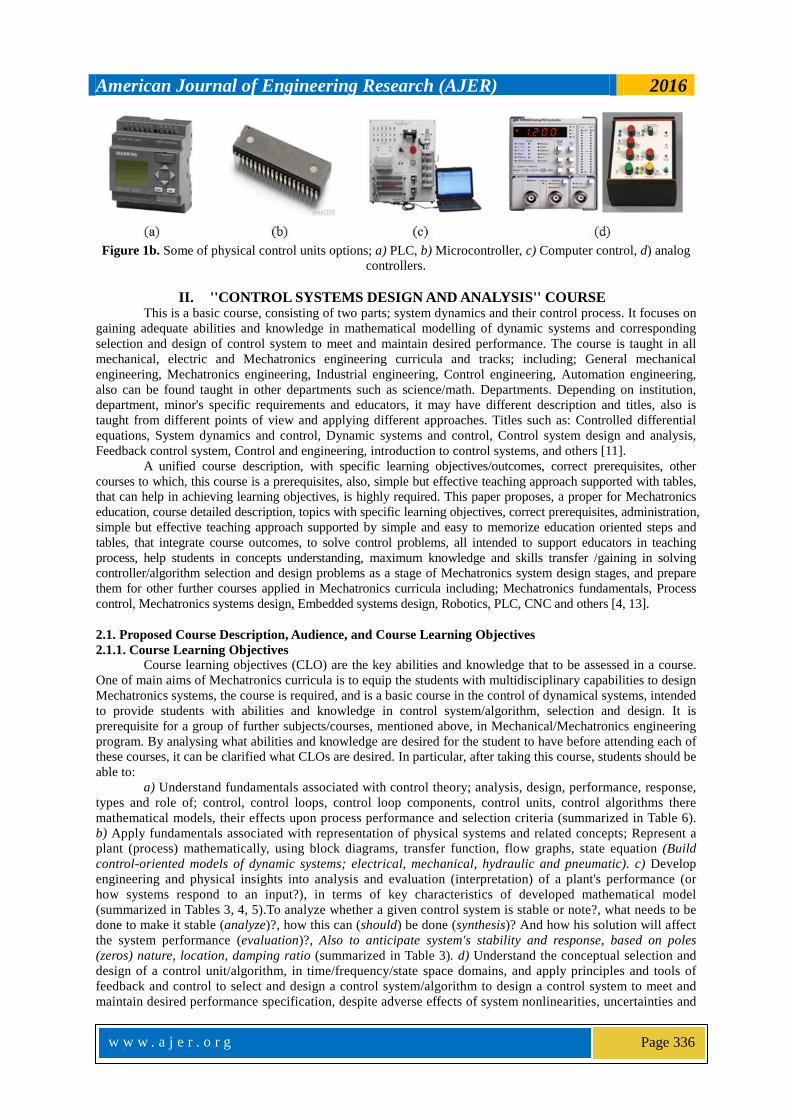
Figure 1b. Some of physical control units options; a) PLC, b) Microcontroller, c) Computer control, d) analog

controllers.

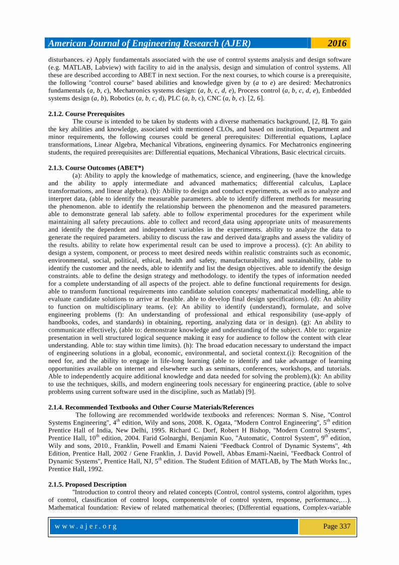
II. ''CONTROL SYSTEMS DESIGN AND ANALYSIS'' COURSE This is a basic course, consisting of two parts; system dynamics and their control process. It focuses on

gaining adequate abilities and knowledge in mathematical modelling of dynamic systems and corresponding

selection and design of control system to meet and maintain desired performance. The course is taught in all

mechanical, electric and Mechatronics engineering curricula and tracks; including; General mechanical

engineering, Mechatronics engineering, Industrial engineering, Control engineering, Automation engineering,

also can be found taught in other departments such as science/math. Departments. Depending on institution,

department, minor's specific requirements and educators, it may have different description and titles, also is

taught from different points of view and applying different approaches. Titles such as: Controlled differential

equations, System dynamics and control, Dynamic systems and control, Control system design and analysis,

Feedback control system, Control and engineering, introduction to control systems, and others [11].

A unified course description, with specific learning objectives/outcomes, correct prerequisites, other

courses to which, this course is a prerequisites, also, simple but effective teaching approach supported with tables,

that can help in achieving learning objectives, is highly required. This paper proposes, a proper for Mechatronics

education, course detailed description, topics with specific learning objectives, correct prerequisites, administration,

simple but effective teaching approach supported by simple and easy to memorize education oriented steps and

tables, that integrate course outcomes, to solve control problems, all intended to support educators in teaching

process, help students in concepts understanding, maximum knowledge and skills transfer /gaining in solving

controller/algorithm selection and design problems as a stage of Mechatronics system design stages, and prepare

them for other further courses applied in Mechatronics curricula including; Mechatronics fundamentals, Process

control, Mechatronics systems design, Embedded systems design, Robotics, PLC, CNC and others [4, 13].

2.1. Proposed Course Description, Audience, and Course Learning Objectives

2.1.1. Course Learning Objectives

Course learning objectives (CLO) are the key abilities and knowledge that to be assessed in a course.

One of main aims of Mechatronics curricula is to equip the students with multidisciplinary capabilities to design

Mechatronics systems, the course is required, and is a basic course in the control of dynamical systems, intended

to provide students with abilities and knowledge in control system/algorithm, selection and design. It is

prerequisite for a group of further subjects/courses, mentioned above, in Mechanical/Mechatronics engineering

program. By analysing what abilities and knowledge are desired for the student to have before attending each of

these courses, it can be clarified what CLOs are desired. In particular, after taking this course, students should be

able to:

a) Understand fundamentals associated with control theory; analysis, design, performance, response,

types and role of; control, control loops, control loop components, control units, control algorithms there

mathematical models, their effects upon process performance and selection criteria (summarized in Table 6).

b) Apply fundamentals associated with representation of physical systems and related concepts; Represent a

plant (process) mathematically, using block diagrams, transfer function, flow graphs, state equation (Build

control-oriented models of dynamic systems; electrical, mechanical, hydraulic and pneumatic). c) Develop

engineering and physical insights into analysis and evaluation (interpretation) of a plant's performance (or

how systems respond to an input?), in terms of key characteristics of developed mathematical model

(summarized in Tables 3, 4, 5).To analyze whether a given control system is stable or note?, what needs to be

done to make it stable (analyze)?, how this can (should) be done (synthesis)? And how his solution will affect

the system performance (evaluation)?, Also to anticipate system's stability and response, based on poles

(zeros) nature, location, damping ratio (summarized in Table 3). d) Understand the conceptual selection and

design of a control unit/algorithm, in time/frequency/state space domains, and apply principles and tools of

feedback and control to select and design a control system/algorithm to design a control system to meet and

maintain desired performance specification, despite adverse effects of system nonlinearities, uncertainties and



Page 337

disturbances. e) Apply fundamentals associated with the use of control systems analysis and design software

(e.g. MATLAB, Labview) with facility to aid in the analysis, design and simulation of control systems. All

these are described according to ABET in next section. For the next courses, to which course is a prerequisite,

the following ''control course'' based abilities and knowledge given by (a to e) are desired: Mechatronics

fundamentals (a, b, c), Mechatronics systems design: (a, b, c, d, e), Process control (a, b, c, d, e), Embedded

systems design (a, b), Robotics (a, b, c, d), PLC (a, b, c), CNC (a, b, c). [2, 6].

2.1.2. Course Prerequisites

The course is intended to be taken by students with a diverse mathematics background, [2, 8]. To gain

the key abilities and knowledge, associated with mentioned CLOs, and based on institution, Department and

minor requirements, the following courses could be general prerequisites: Differential equations, Laplace

transformations, Linear Algebra, Mechanical Vibrations, engineering dynamics. For Mechatronics engineering

students, the required prerequisites are: Differential equations, Mechanical Vibrations, Basic electrical circuits.

2.1.3. Course Outcomes (ABET*)

(a): Ability to apply the knowledge of mathematics, science, and engineering, (have the knowledge

and the ability to apply intermediate and advanced mathematics; differential calculus, Laplace

transformations, and linear algebra). (b): Ability to design and conduct experiments, as well as to analyze and

interpret data, (able to identify the measurable parameters. able to identify different methods for measuring

the phenomenon. able to identify the relationship between the phenomenon and the measured parameters.

able to demonstrate general lab safety. able to follow experimental procedures for the experiment while

maintaining all safety precautions. able to collect and record data using appropriate units of measurements

and identify the dependent and independent variables in the experiments. ability to analyze the data to

generate the required parameters. ability to discuss the raw and derived data/graphs and assess the validity of

the results. ability to relate how experimental result can be used to improve a process). (c): An ability to

design a system, component, or process to meet desired needs within realistic constraints such as economic,

environmental, social, political, ethical, health and safety, manufacturability, and sustainability, (able to

identify the customer and the needs, able to identify and list the design objectives. able to identify the design

constraints. able to define the design strategy and methodology. to identify the types of information needed

for a complete understanding of all aspects of the project. able to define functional requirements for design.

able to transform functional requirements into candidate solution concepts/ mathematical modelling, able to

evaluate candidate solutions to arrive at feasible. able to develop final design specifications). (d): An ability

to function on multidisciplinary teams. (e): An ability to identify (understand), formulate, and solve

engineering problems (f): An understanding of professional and ethical responsibility (use-apply of

handbooks, codes, and standards) in obtaining, reporting, analyzing data or in design). (g): An ability to

communicate effectively, (able to: demonstrate knowledge and understanding of the subject. Able to: organize

presentation in well structured logical sequence making it easy for audience to follow the content with clear

understanding. Able to: stay within time limits). (h): The broad education necessary to understand the impact

of engineering solutions in a global, economic, environmental, and societal context.(i): Recognition of the

need for, and the ability to engage in life-long learning (able to identify and take advantage of learning

opportunities available on internet and elsewhere such as seminars, conferences, workshops, and tutorials.

Able to independently acquire additional knowledge and data needed for solving the problem).(k): An ability

to use the techniques, skills, and modern engineering tools necessary for engineering practice, (able to solve

problems using current software used in the discipline, such as Matlab) [9].

2.1.4. Recommended Textbooks and Other Course Materials/References

The following are recommended worldwide textbooks and references: Norman S. Nise, ''Control

Systems Engineering'', 4th

edition, Wily and sons, 2008. K. Ogata, ''Modern Control Engineering'', 5th

edition

Prentice Hall of India, New Delhi, 1995. Richard C. Dorf, Robert H Bishop, ''Modern Control Systems'',

Prentice Hall, 10th

edition, 2004. Farid Golnarghi, Benjamin Kuo, ''Automatic, Control System'', 9th

edition,

Wily and sons, 2010., Franklin, Powell and Emami Naieni ''Feedback Control of Dynamic Systems'', 4th

Edition, Prentice Hall, 2002 / Gene Franklin, J. David Powell, Abbas Emami-Naeini, ''Feedback Control of

Dynamic Systems'', Prentice Hall, NJ, 5th

edition. The Student Edition of MATLAB, by The Math Works Inc.,

Prentice Hall, 1992.

2.1.5. Proposed Description

''Introduction to control theory and related concepts (Control, control systems, control algorithm, types

of control, classification of control loops, components/role of control system, response, performance,…).

Mathematical foundation: Review of related mathematical theories; (Differential equations, Complex-variable



Page 338

theory and Laplace & z-transforms). System representation; mathematical modelling represent physical systems

(electrical, mechanical, hydraulic and pneumatic) using the following forms; differential equations, Block

diagrams (and corresponding algebra), transfer function (poles, zeros, pole zero map), state space equation, and

signal flow graphs (Mason’s gain formula). Analysis and evaluation of system (plant) performance (transient

and steady state response measures of I and II order system, dominant poles of higher order systems). Selection

and design of control system/compensators in time domain, to meet and maintain desired overall system

performance. Analysis and design in frequency domain. Analysis and design in state space domain''. Control

systems analysis and design software (e.g. MATLAB, Labview) with facility to aid in the analysis, design and

simulation of control systems, (MATLAB built-in function for analysis and plotting systems' response,

Introduce control system toolbox sisotool and rltool and corresponding design and analysis) [9].

2.1.6. Proposed Simple and Easy to Memorized and Follow Control System Design Teaching Approach,

To support educators in knowledge delivery, and help students in achieving CLOs abilities and

knowledge and solve control problems, the course topics and CLOs/outcomes are organized and integrated in

simple and easy to memorized and follow steps, to select and design a control system to meet and maintain a

desired performance. These steps are shown in Figure 2. Depending on institution, Department and minor,

educator's back ground, these steps are given in different forms/details, shown in Figures 2a, b, c.

To evaluate concepts and gain required associated integrated abilities and knowledge desired for further

courses, the description and the teaching approach, are supported with tables (1c: 7) and graphs, that are

recommended to provide students with, and ask to bring on every lecture, where: In Table 1, the proposed

course description and topics is explained in details, in particular, main topics mapped with their specific

subtitles, objectives, number of lectures and weeks. In Table 2: Some basic rules of block diagram algebra. In

Table 3a,b first and second order systems modelling, response measures and general forms of transfer function.

In Table 3c the nature of second order system poles (roots) and the effect of changing damping and undamped

natural frequency on systems response. In Table 4: the steady state error dependence on input signal and system

type. In table 5 Control systems/algorithms transfer function, actions, selection criteria and root locus sketching

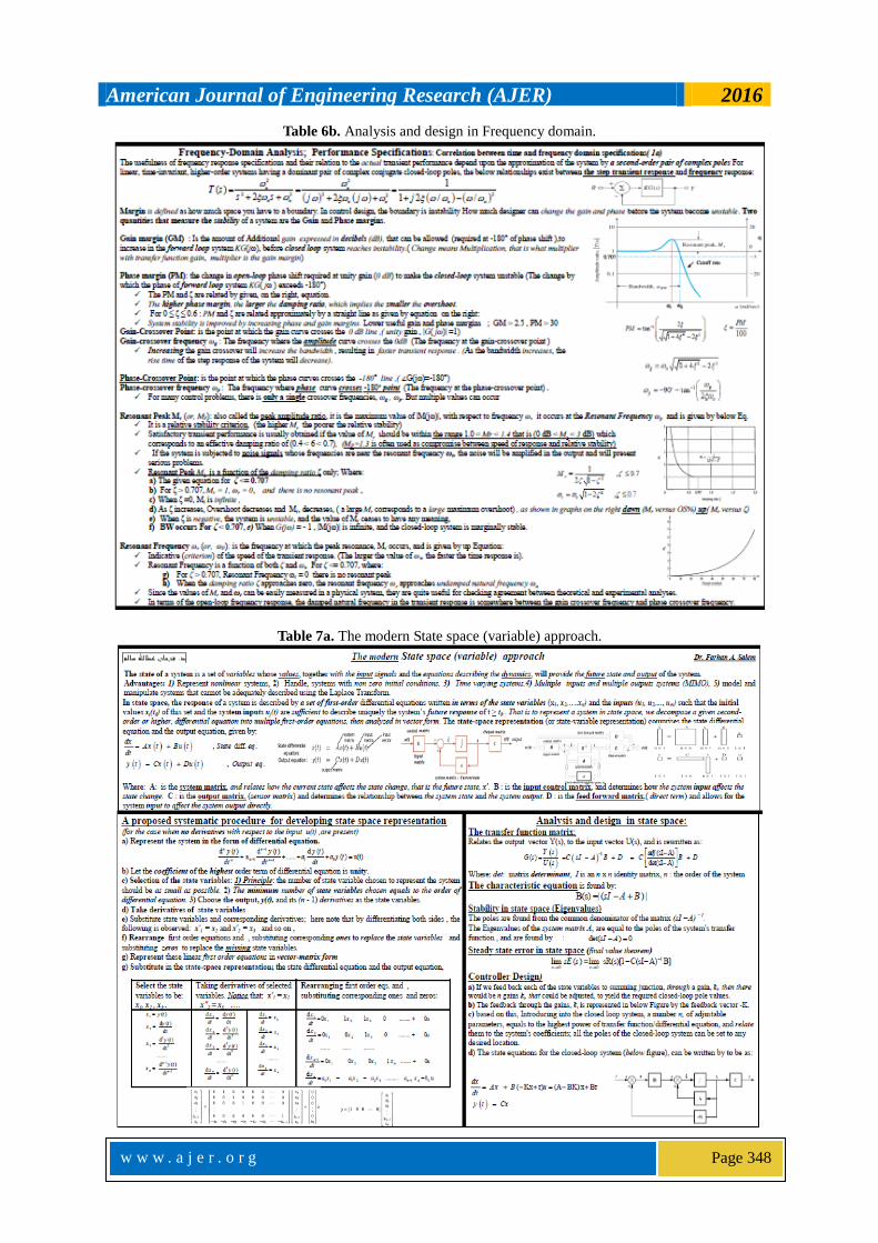
rules. Table 6 analysis and design in Frequency domain [12]. Table 7 analysis and design- the modern State

space (variable) approach. [10].

2.1.7. Recommend Course Administration

The course is taught in 14/15 weeks, with two (I and II) midterm exams, 3 Lab session (to convey

concepts when possible, along with simulations and interactive MATLAB sessions), Course Project,

Homework sets, and a final exam.

2.1.8. Class Schedule

4 Credits hours, (4: 2, 1, 1): 100-minutes lecture per week, 100-minutes tutorial per week, and 150-minutes

laboratory hours every three weeks:

Table 1a. Class schedule. Activity Name Hours per Week Sessions per Week Weeks per Semester

Lecture 2 1 14

Tutorial 2 1 14

Labs 3/every three weeks 1/every three weeks 3

2.1.9. Recommended Grading System

Table 1b. Recommended grading system. Class performance (Atten., particip., assignments) 10%

Labs (3) 15%

Quizzes/ Tests (3-5) 10%

First Exam I 10%

Second exam II 10%

Project; Written/Oral; (Report + Presentation) 15%

Final 30%

Total 100%

2.1.10. Pre-course

A special pre-course recommended to be offered in the week before the course begins. This pre-course

gives a concise introduction to four main topics: linear algebra, ordinary differential equations, complex theory

and dynamical systems.



Page 339

III. TEACHING PLAN AND TOPICS EXPLAINED Table 1c. Teaching plan and explained topics of the course.

Topics to be covered

1) Introduction to control theory and related concepts.

(T1:1, 1, 2): First Week, 1 Lecture, 2 Hours. a) Course overview: first day materials; describe course structure, objectives, administration,.

b) Definition of main control concepts and terminologies; Control, control system, Controller, control algorithm, control system

components; Sensor, Actuator, Plant, Process. Input, output, disturbance, test input signals, response and plots (transient & steady state), performance, steady state error, performance evaluation, Control low, Design, Analysis, Control history.

c) Advantages of control systems and application examples.

d) Definition and classifications/types of each of: Control (automatic and manual), Processes (SISO, MIMO), Control systems (Discrete (ON/Off), Multistep, Continuous (P-, PI, PD, PID, Lead, Lag…)), control loops (A single variable control loop

(Feedback, Feedforward), Multivariable Control loop (Feedback plus Feedforward, cascade control, ratio control)).

e) Introduce (proposed) steps for control system selection and design Figure 2a, b, c. f) Introduce role of control systems analysis and design software (e.g. MATLAB, Labview) to aid in the analysis, design and

simulation of control systems.

2) Mathematical foundation: Review of related mathematical theories; differential equations, Complex-variable theory and Laplace

transform.

(T2:1, 1, 2): First week, 1 lecture, 2 hours.

a) Ordinary differential equations (First and Second order HODE, solving/ plotting solution, relating differential equation terminologies with control system terminologies (e.g. solution/response, particular integrate/transient response, forced

function/steady state response, characteristic equation …).

b) Complex variables (complex plane, complex conjugate, phase, magnitude, Complex Arithmetic. c) Laplace transform and elements of the Laplace transform (Laplace table)

3) System representation-mathematical modelling: represent physical systems (electrical, mechanical, hydraulic and pneumatic) using

differential equations, Block diagrams, transfer function, state space equation, and signal flow graphs.

(T3:2-4, 5, 10): II by IV Week, 5 Lectures, 10 Hours. a) Introducing I & II order systems, why in control engineering, we most interested in study of such systems?.

b) Modeling basics and definition of concepts. Forms of mathematical models;(differential equations, state space equations, transfer

function, block diagrams...). Developing mathematical model in the form of differential equations for mechanical systems (translational, rotational, and combination, mechanical elements; Spring, Mass, Damper), Electric systems (circuits & elements;

resistor, capacitor, inductor RC, RLC circuits), electromechanical (DC motor), hydraulic and pneumatic systems, including; First

order systems (car spring-damper suspension system, car cruise control, tank level control, pressure control, RC circuit), and Second order systems (Two tank system, Spring-mass-damper…), higher order system (e.g. DC motor, Two-degrees-of freedom

system), analogies.

c) Linearization of nonlinear systems. d) Representing system using state equations. Concepts, definition and equations development.

e) Representing system using Block diagram and Block diagram algebra; block diagrams reduction techniques (Table 2),

Representing system using signal flow graphs, Mason’s gain formula. f) Representing system using transfer function: forward, open loop, closed loop, overall transfer function, Poles, Zeros, Pole-Zero

map.

(Most of proposed is recommended to be taught in parallel, e.g. derive mathematical model of a given system in the form of differential equation, (and/or write state equations), apply Laplace transform, develop transfer function, find Poles, Zeros, and plot

pole-zero map.

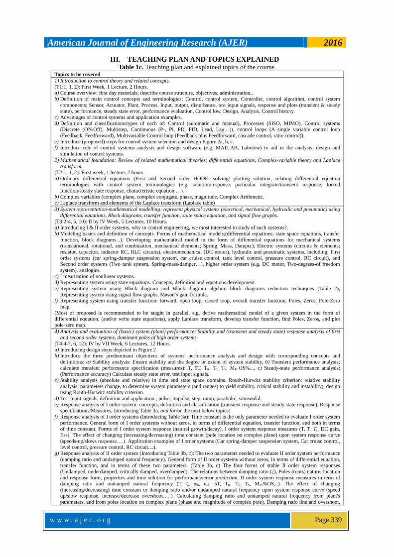
4) Analysis and evaluation of (basic) system (plant) performance; Stability and (transient and steady state) response analysis of first and second order systems, dominant poles of high order systems.

(T4:4-7, 6, 12): IV by VII Week, 6 Lectures, 12 Hours.

a) Introducing design steps depicted in Figure 2 b) Introduce the three predominant objectives of systems' performance analysis and design with corresponding concepts and

definitions; a) Stability analysis: Ensure stability and the degree or extent of system stability, b) Transient performance analysis;

calculate transient performance specification (measures): T, 5T, TR, TP, TS, MP, OS%..., c) Steady-state performance analysis; (Performance accuracy) Calculate steady state error, test input signals.

c) Stability analysis (absolute and relative) in time and state space domains. Routh-Hurwitz stability criterion: relative stability

analysis: parameters change, to determine system parameters (and ranges) to yield stability, critical stability and instability), design using Routh-Hurwitz stability criterion.

d) Test input signals, definition and application.; pulse, impulse, step, ramp, parabolic, sinusoidal.

e) Response analysis of I order system: concepts, definition and classification (transient response and steady state response). Response specifications/Measures, Introducing Table 3a, and for/or the next below topics:

f) Response analysis of I order systems (Introducing Table 3a): Time constant is the only parameter needed to evaluate I order system

performance. General form of I order systems without zeros, in terms of differential equation, transfer function, and both in terms of time constant. Forms of I order system response (natural growth/decay). I order system response measures (T, Tr, Ts, DC gain,

Ess). The effect of changing (increasing/decreasing) time constant (pole location on complex plane) upon system response curve

(speeds-up/slows response….). Application examples of I order systems (Car spring-damper suspension system, Car cruise control, level control, pressure control, RC circuit....).

g) Response analysis of II order system (Introducing Table 3b, c): The two parameters needed to evaluate II order system performance

(damping ratio and undamped natural frequency). General form of II order systems without zeros, in terms of differential equation, transfer function, and in terms of these two parameters. (Table 3b, c) The four forms of stable II order system responses

(Undamped, underdamped, critically damped, overdamped). The relations between damping ratio (ξ), Poles (roots) nature, location

and response form, properties and time solution for performance/error prediction. II order system response measures in term of damping ratio and undamped natural frequency (T, ζ, ωn, ωd, 5T, TR, TP, TS, MP,%OS,..). The effect of changing

(increasing/decreasing) time constant or damping ratio and/or undamped natural frequency upon system response curve (speed up/slow response, increase/decrease overshoot…..). Calculating damping ratio and undamped natural frequency from plant's

parameters, and from poles location on complex plane (phase and magnitude of complex pole). Damping ratio line and overshoot,



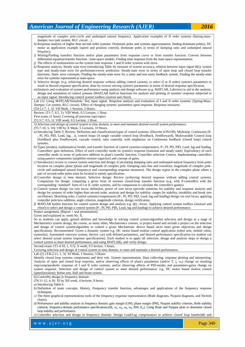
Page 340

magnitude of complex pole-circle and undamped natural frequency. Application examples of II order systems (Spring-mass-

damper, two tank system, RLC circuit…). h) Response analysis of higher than second order systems: Dominant poles and systems approximation, finding dominant pole(s), DC

motor as application example (speed and position control), dominant poles in terms of damping ratio and undamped natural

frequency. i) Writing/Finding transfers function and/or plant parameters from response curve or from transfer function. Convert between

differential equation/transfer function / state-space models. Finding time response from the state-space representation.

j) The effects of nonlinearities on the system time response. I and II order systems with zeros. k) Response analysis; Steady state error (introducing Table 4): measure of system accuracy, relation between input signal R(s), system

type and steady-state error for performance/error prediction. Steady-state error in terms of open loop and closed loop transfer

functions. Static error constants. Finding the steady-state error for a unity and non unity feedback system. Finding the steady-state error for systems represented in state-space.

l) Selective design: (e.g. achieving desired response without adding control system), to select (I or II order) system's parameters to

result in desired response specification, done by reverse solving system's parameters in terms of desired response specification. m) Analysis and evaluation of system performance using analysis and design software (e.g. MATLAB, Labview) to aid in the analysis,

design and simulation of control systems (MATLAB built-in functions for analysis and plotting of systems' response subjected to

an input signal. Introducing control system toolbox sisotool and rltool).

Lab (1): Using MATLAB/Simulink: Test input signal. Response analysis and evaluation of I and II order systems' (Spring-Mass-

Damper, Car system, RLC circuit). Effect of changing systems' parameters upon response. Response measures.

(T4-L1:7, 1, 3): VII Week, 1 Session, 3 Hours.

Review: (T1-7, 0.5, 1): VIII Week, 0.5 Lecture, 1 Hour. First exam: (1 hour): Covering all previous (up) topics

(T1:5:7, 0.5, 1): VIII week, 0.5 Lecture, 1 Hour.

5) Selection and design of control system in time domain, to meet and maintain desired overall system performance. (T5:7-10, 5, 10): VIII by X Week, 5 Lectures, 10 Hours.

a) Introducing Table 5: Review: Definition and classifications/types of control systems; (Discrete (ON/Off), Multistep, Continuous (P-

, PI, PD, PID, Lead, lag…)), control loops (A single variable control loop (Feedback, Feedforward), Multivariable Control loop (Feedback plus Feedforward, cascade control, ratio control)), with emphasize on Continuous feedback (closed loop) control

systems.

b) Types (modes), mathematical model, and transfer function of control systems/compensators; P-, PI, PD, PID, Lead, lag and leadlag. Controllers' gain definition. Effect of each controller mode on system's response (transient and steady state). Equivalency of each

controller mode in terms of pole/zero addition to plant's transfer function. Controller selection Criteria. Implementing controllers

using passive components (amplifier-resistor-capacitor) and concept of gains. c) Introductory review to control system selection and design: (Calculating damping ratio and undamped natural frequency from poles

location on complex plane (phase and magnitude of complex pole. Damping ratio line and overshoot, magnitude of complex pole-

circle and undamped natural frequency) and corresponding response measures). The design region in the complex plane where a pair of second-order poles must be located to satisfy specification.

d) Controller design in time domain: Selective design: Review (achieving desired response without adding control system).

Comparison for design: comparing a given form of systems closed-loop transfer function (e.g. with P-controller) with the corresponding "standard" form of I or II -order systems, and by comparison to calculate the controller's gain(s).

e) Control system design via root locus; definition, power of root locus (provide solutions for stability and response analysis and

design for systems of order higher than second order, analysis and design for stability; ranges for stability, instability and break into oscillation). Sketching rules. Control systems/compensators (P-, PI, PD, PID, Lead, lag and leadlag) design via root locus; applying

controller pole/zero addition, angle criterion, magnitude criterion, design verification.

f) MATLAB builtin function for control system design and analysis e.g. tf(), rlocus. Applying control system toolbox (sisotool and rltool) to select and design a control system (P-, PI, PD, PID, Lead, lag and leadlag) to achieve desired performance.

Project assignment, (Report + oral presentation):

Given and explained in: week No. X. So as students can apply, gained abilities and knowledge in solving control system/algorithm selection and design as a stage of

Mechatronics system design, the course, as many other, Mechatronics courses, is project-based and include a project on the selection

and design of control system/algorithm to control a given Mechatronic device based on/to meet given objectives and design specifications. Recommended: Given a dynamic system e.g. DC motor based motion control application (robot arm, mobile robot,

suntracker, Automated conveyer system, electric car) with defined parameters, and desired performance specification (or student can

select desired actual system response specifications). Each student is to apply all selection, design and analysis steps to design a control system to meet desired performance, and using MATLAB), and verify design.

Second exam: (T1-4:10, 1, 0.5): X week, 0.5 lecture, 1 hours.

Covering selection and design of control system in time domain, to meet and maintain a desired performance.

Lab (2): (T4L2:11, 1, 3): XI Week, 1 Session, 3 Hours Identify closed loop systems components and their role. System representation. Data collecting, response plotting and interpreting:

Analysis of open and closed loop response, and/or observing effects of plant's parameters (and/or T, ζ, ωn) change on resulting

step/ramp/parabolic response of I and II order systems, and/or observing effects of PID-modes and parameters-gains change on system response. Selection and design of control system to meet desired performance: e.g. DC motor based motion control

(speed/position); Robot arm, Ball and beam system.

6) Controller design in frequency domain: (T6:11-12, 4, 8): XI by XII week, 4 lectures, 8 hours.

a) Introducing Table 6.

b) Definition of main concepts; History, Frequency transfer function, advantages and applications of the frequency response techniques.

c) The three graphical representations tools of the frequency response representation (Bode diagrams, Nyquist diagrams, and Nichols

charts). d) Performance and stability analysis in frequency domain; gain margin (GM), phase margin (PM), Nyquist stability criterion, Bode stability

criterion, frequency-domain performance specifications;(Mr, ωr, ωp, ωg, ωb, BW, Ess). Using Bode and Nyquist plots to determine closed

loop stability and performance. e) Controller selection and design in frequency domain: Design Lead/Lag compensators to achieve closed loop bandwidth and



Page 341

stability margins

7) Introduction to analysis and design in state-space:

(T7:13, 2, 4): XIII week, 2 lectures, 4 hours. a) Introducing Table 7,

b) The general state-space representation,

c) Stability analysis in state space, d) Steady-state error for systems in state space,

e) Controller design in state space (pole placement)

Lab (3): frequency response (T4L3:14, 1, 3): XIV Week, 1 session, 3 Hours.

Course Project defense: (Report + Oral)

(T1-7:14, 1, 2): XIV Week, 1 Lecture, 2 Hours.

Course Review of; objectives / gained abilities and knowledge, Selection and design examples, relation to other subjects. (T1-7:14, 1, 2): XIV week, 1 lecture, 2 hours.

TOTAL: 7 Topics, 15 weeks, 28 lectures, 2 lectures for Midterms +quizzes, 60 hours, 3 Lab sessions 9 hours.

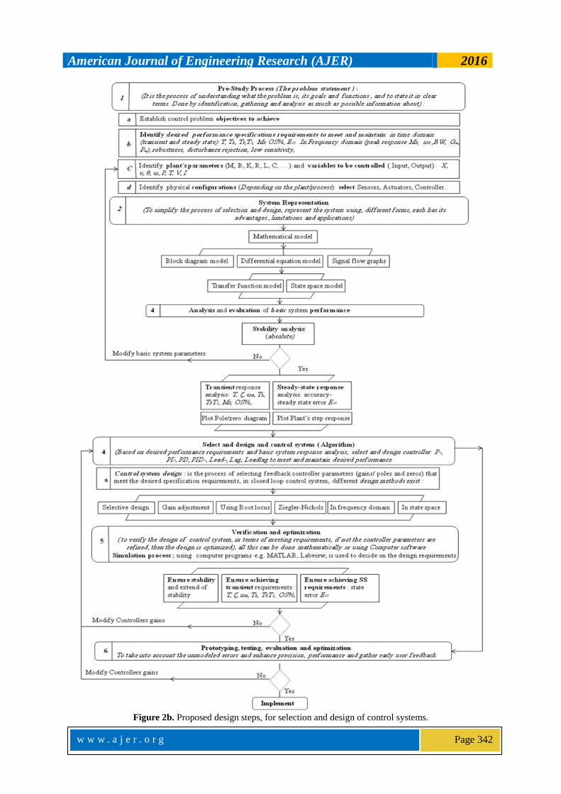
Pre-Study Process (The problem statement ) :

(It is the process of understanding what the problem is, its goals and functions , and to state it in clear terms. Done by identification, gathering and analysis as much as possible information about) :

1

System Representation

(To simplify the process of selection and design, represent the system using, different forms, each has its advantages , limitations and applications)

2

Reduce whole system block diagram model; (apply block diagram algebra)3

Solve mathematical model and plot the solution ( response) of ( differential equation or transfer function, or

state space model), subject the system to test input signal ( step, ramp, parabolic, sinusoidal….), Analyze

and Evaluate resulted, the three predominant objectives of systems analysis and evaluation are

a

Select and design and control system ( Algor ithm)

(Based on desired ( performance) requirements and basic system response analysis, select and design controller: P-, PI-, PD, PID-, Lead-, Lag, Leadlag;)

4

a

Prototyping, testing, evaluation and optimization

To take into account the unmodeled errors and enhance precision, performance and gather early user feedback6

Manufactur ing and Commercialization7 Support, Service and Market feedback Analysis 8

Step

s for

cont

rol s

ystem

selec

tion

and

desig

n

Establish control problem objectives to achievea

Simulation process ; using computer programs e.g. MATLAB, Labview, is used to decide on the design

requirements.

Requirements

analysis and

identifications

b

Functional requirements: what is system’s major function to perform?, is it performing it?

Performance requirements: How well the system does what it is suppose to do?

Desired performance specifications requirements to meet and maintain : in time domain (transient and steady state): T, TR, TP,TS, MP, OS%, ESS. . In Frequency domain (peak response MP, ωP ,BW, Gm, Pm), robustness, disturbance rejection, low sensitivity,

Environmental requirements: Under what conditions, does the system have to work and

meet performance goals?

Identify physical configurations (Depending on the plant/process): select Sensors, Actuators, Controller.. d

Develop (draw) physical model: based on objectives and requirements, describe the physical system in

terms of principle of working, components and interconnections, to simplify the picture some phenomena

can be neglected/ approximateda

b

Develop (draw) functional block diagram model: translate objective, physical model, and qualitative

description, into functional block diagram describing components, subsystems (sensors, actuators, controller,

amplifier,..) interconnections, inputs, outputs, math. model of each component can be placed in each blocks

c

Develop mathematical (differential equations) model: using physical law (Newton’s, Kirchhoff's, …) to

represent (model) each components/subsystem, then according to developed block diagram model, develop

whole system mathematical model with input and output as identified in step (1-c)

each subsystem/component is represented using block diagram with input and output , these then connected

to develop whole system block diagram model.

Differential equation model Transfer function modelBlock diagram model State space model

Simplicity VS accuracy: the more accurate the mathematical description of each subsystem, the more

complex the modeling equations are. It is necessary to ignore a certain inherent physical properties of

system, it is desirable to first built simplified model, later more accurate model for accurate analysis is built

d

Develop mathematical transfer function model: only applied for linear systems, and is defined as the

ratio of the Laplace transform of the output to the Laplace transform of the input, represented by G(s),

transfer function gives more intuitive information than differential equation, and useful in modeling

interconnections, and rapidly sense the effect of parameters change

e Develop mathematical state space model: applied for systems that can‘t be represented using lineardifferential equations ( by transfer function),also are used to model systems for simulation on computer

a

Applying block diagram algebra, whole system block diagram, with all subsystem’s models ( sensor,

actuator, dynamics…) is simplified to single block model, with one mathematical model ( or one transfer

function), that represent the whole system from input to output

4 Analysis and evaluation of basic system performance

Physical model Schematic model Mathematical model

Signal flow

Stability analysis: absolute ( is the system stable (all

pole’s real part are negative? Yes, No) & relative stab.(using Routh-Horwitz criterion, plot pole zero diagram.

Transient response

analysis: T, TR, TP,TS, MP, OS%,.

Steady-state response

analysis: accuracy-

steady state error ESS

Based on calculated response measures (T, TR, TP,TS, MP, OS%, Ess), plot response curve and evaluate responseb

Gain adjust. Using RlocusSelective design Ziegler-Nichols

aControl system design : is the process of selecting feedback controller parameters (gains/poles/zeros) that meet

& maintain the desired specification requirements, in closed loop control system, different design methods exist :

In state spaceIn frequency domain

Verification and optimization

( to verify the design of control system, in terms of meeting requirements, if not the controller parameters are refined, then the design is optimized), all this can be done mathematically or using Computer software

5

Identify plant’s parameters (M, B, K, R, L, C, ….) and var iables to be controlled ( Input, Output): X, υ, θ, ω, P, T, V, I

C

P. Placement

Figure 2a. Course proposed design steps, for selection and design of control systems.



Page 342

Figure 2b. Proposed design steps, for selection and design of control systems.



Page 343

Pre-Study Process (The problem statement )

Identify var iables to be controlled ( Input,

Output): X, υ, θ, ω, P, T, V, I

System Representation

Select and design and control system ( Algor ithm)

Prototyping, testing, evaluation and optimization

To take into account the unmodeled errors and enhance precision, performance and gather early user feedback.

Implement

Establish control problem objectives to achieve

Identify physical configurations (Depending on the plant/process

select Sensors, Actuators, amplifier……. and parameters)

Differential equation model

Transfer function model

Block diagram model

State space model

Physical model

Schematic model

Mathematical model

Signal flow graph model

In state space

Testing &Verification of Control system selection & design, meeting

requirements? (Mathematically or using computer simulation( e.g. MATLAB)

Identify desired performance specifications

requirements to meet and maintain

In time domain (transient and steady

state): T, TR, TP,TS, MP, OS%, ESS.

In Frequency domain(peak response

MP, ωP ,BW, Gm, Pm),

TF frequency model

Analysis and evaluation

Transient response analysis

Stability analysis

Steady state response analysis

No

Yes

Modify basic system parameters

P-, PI-, PD, PID-, Lead-, Lag, Leadlag

Gain adjustment Using Root locusSelective design Ziegler-Nichols In frequency domain

Plot Root locus

Find Dominant pole(s) from desired response specification

(transient and steady state): T, TR, TP,TS, MP, OS%, ESS.

Apply angle and magnitude cr iter ions to select gains

Bode plots

Nyquist diagram

Nichols charts

No

Yes

Refine controller parameters,

Ensure achieving desired

Transient response

Ensuring Stability Ensure achieving desired

steady state response

Robustness Disturbance rejection Low sensitivity

No

Yes

Refine controller parameters,

Mr, ωr , BW, ωb ,CR

Select Controller’s gains

Figure 2c. Flowchart; proposed design steps, for selection and design of control systems.



Page 344

Table 2. Some basic rules of block diagram algebra [3].

Table 3a. I order systems modelling, response analysis, Performance measures, control loop, and general forms

of transfer function G(s).



Page 345

Table 3b. II order systems modelling, response analysis, Performance measures and general forms of transfer

function G(s).

Table 3c. The nature of second order system poles (roots) and the effect of changing damping and undamped

natural frequency on systems response.



Page 346

Table 4. The steady state error dependence on input signal and system type.

Table 5a. Control systems/algorithms transfer function, actions, selection criteria.



Page 347

Table 5b. Control algorithm design via root locus.

Table 6a. Analysis and design in Frequency domain.



Page 348

Table 6b. Analysis and design in Frequency domain.

Table 7a. The modern State space (variable) approach.



Page 349

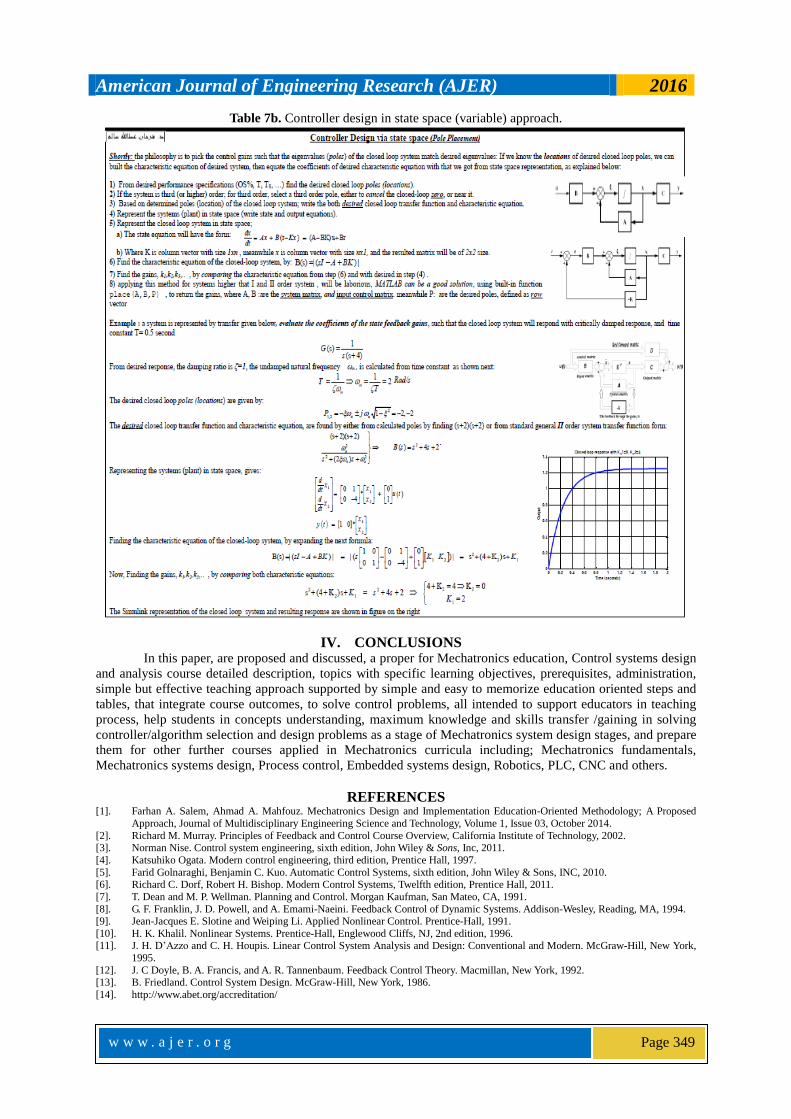
Table 7b. Controller design in state space (variable) approach.

IV. CONCLUSIONS In this paper, are proposed and discussed, a proper for Mechatronics education, Control systems design

and analysis course detailed description, topics with specific learning objectives, prerequisites, administration,

simple but effective teaching approach supported by simple and easy to memorize education oriented steps and

tables, that integrate course outcomes, to solve control problems, all intended to support educators in teaching

process, help students in concepts understanding, maximum knowledge and skills transfer /gaining in solving

controller/algorithm selection and design problems as a stage of Mechatronics system design stages, and prepare

them for other further courses applied in Mechatronics curricula including; Mechatronics fundamentals,

Mechatronics systems design, Process control, Embedded systems design, Robotics, PLC, CNC and others.

REFERENCES [1]. Farhan A. Salem, Ahmad A. Mahfouz. Mechatronics Design and Implementation Education-Oriented Methodology; A Proposed

Approach, Journal of Multidisciplinary Engineering Science and Technology, Volume 1, Issue 03, October 2014.

[2]. Richard M. Murray. Principles of Feedback and Control Course Overview, California Institute of Technology, 2002. [3]. Norman Nise. Control system engineering, sixth edition, John Wiley & Sons, Inc, 2011.

[4]. Katsuhiko Ogata. Modern control engineering, third edition, Prentice Hall, 1997.

[5]. Farid Golnaraghi, Benjamin C. Kuo. Automatic Control Systems, sixth edition, John Wiley & Sons, INC, 2010. [6]. Richard C. Dorf, Robert H. Bishop. Modern Control Systems, Twelfth edition, Prentice Hall, 2011.

[7]. T. Dean and M. P. Wellman. Planning and Control. Morgan Kaufman, San Mateo, CA, 1991.

[8]. G. F. Franklin, J. D. Powell, and A. Emami-Naeini. Feedback Control of Dynamic Systems. Addison-Wesley, Reading, MA, 1994. [9]. Jean-Jacques E. Slotine and Weiping Li. Applied Nonlinear Control. Prentice-Hall, 1991.

[10]. H. K. Khalil. Nonlinear Systems. Prentice-Hall, Englewood Cliffs, NJ, 2nd edition, 1996. [11]. J. H. D’Azzo and C. H. Houpis. Linear Control System Analysis and Design: Conventional and Modern. McGraw-Hill, New York,

1995.

[12]. J. C Doyle, B. A. Francis, and A. R. Tannenbaum. Feedback Control Theory. Macmillan, New York, 1992. [13]. B. Friedland. Control System Design. McGraw-Hill, New York, 1986.

[14]. http://www.abet.org/accreditation/

Systems Dynamics and Control, Proposed Course …ajer.org/papers/v5(12)/ZR05120334349.pdf ·...

Documents

Transcript of Systems Dynamics and Control, Proposed Course …ajer.org/papers/v5(12)/ZR05120334349.pdf ·...