SYSTEMIC CRISES AND GROWTH - UCLA · PDF fileSYSTEMIC CRISES AND GROWTH Romain Ranciere Aaron...
41
SYSTEMIC CRISES AND GROWTH Romain Ranciere Aaron Tornell Frank Westermann May 13, 2007. Forthcoming Quarterly Journal of Economics Abstract Countries that have experienced occasional nancial crises have, on average, grown faster than countries with stable nancial conditions. Because nancial crises are realizations of down- side risk, we measure their incidence by the skewness of credit growth. Unlike variance, negative skewness isolates the impact of the large, infrequent and abrupt credit busts associated with crises. We nd a robust negative link between skewness and GDP growth in a large sample of countries over 1960-2000. This suggests a positive e/ect of systemic risk on growth. To explain this nding, we present a model in which contract enforceability problems generate borrowing constraints and impede growth. In nancially liberalized economies with moderate contract enforceability, systemic risk taking is encouraged and increases investment. This leads to higher mean growth, but also to greater incidence of crises. In the data, the link between skewness and growth is indeed strongest in such economies. JEL Classication No. F34, F36, F43, O41. Key Words: Financial-Liberalization, Globalization, Lending-Booms, Skewness, Systemic-Risk, Volatility. We thank Christopher Barr, Jess Benhabib, Ariel Burstein, Mike Callen, Roberto Chang, Antonio Ciccone, Daniel Cohen, Carl-Johan Dalgaard, Raquel Fernandez, Bob Flood, Pierre Gourinchas, Thorvaldur Gylfason, Jürgen von Hagen, Lutz Hendricks, Olivier Jeanne, Kai Konrad, Andrei Levchenko, Paolo Mauro, Fabrizio Perri, Thomas Piketty, Joris Pinkse, Assaf Razin, Carmen Reinhart, Thomas Sargent, Hans-Werner Sinn, Carolyn Sissoko, Thierry Tressel, Jaume Ventura, Fabrizio Zilibotti, and seminar participants at Bonn, DELTA, ESSIM, ECB, Harvard, IIES, IMF, Munich, NBER and NYU for helpful comments. We also thank the editor, Robert Barro, and three anonymous referees for valuable suggestions. Katja Drechsel, Chiarra Sardelli, and Mary Yang provided excellent research assistance. The views expressed herein are those of the authors and should not be attributed to the IMF, its Executive Board, or its management. Financial support from UC Mexus-Conacyt for Tornell and from the Ministerio de Ciencia y Tecnologia (SEC2004-03619) for Ranciere are gratefully acknowledged. The appendix to this paper can be dowloaded at http://www.romainranciere.com/unpublished_appendix1.pdf
Transcript of SYSTEMIC CRISES AND GROWTH - UCLA · PDF fileSYSTEMIC CRISES AND GROWTH Romain Ranciere Aaron...
SYSTEMIC CRISES AND GROWTH �
Romain Ranciere Aaron Tornell Frank Westermann
May 13, 2007.
Forthcoming Quarterly Journal of Economics
Abstract
Countries that have experienced occasional �nancial crises have, on average, grown faster
than countries with stable �nancial conditions. Because �nancial crises are realizations of down-
side risk, we measure their incidence by the skewness of credit growth. Unlike variance, negative
skewness isolates the impact of the large, infrequent and abrupt credit busts associated with
crises. We �nd a robust negative link between skewness and GDP growth in a large sample of
countries over 1960-2000. This suggests a positive e¤ect of systemic risk on growth. To explain
this �nding, we present a model in which contract enforceability problems generate borrowing
constraints and impede growth. In �nancially liberalized economies with moderate contract
enforceability, systemic risk taking is encouraged and increases investment. This leads to higher
mean growth, but also to greater incidence of crises. In the data, the link between skewness and
growth is indeed strongest in such economies.
JEL Classi�cation No. F34, F36, F43, O41.
Key Words: Financial-Liberalization, Globalization, Lending-Booms, Skewness, Systemic-Risk,
Volatility.
�We thank Christopher Barr, Jess Benhabib, Ariel Burstein, Mike Callen, Roberto Chang, Antonio Ciccone,Daniel Cohen, Carl-Johan Dalgaard, Raquel Fernandez, Bob Flood, Pierre Gourinchas, Thorvaldur Gylfason, Jürgenvon Hagen, Lutz Hendricks, Olivier Jeanne, Kai Konrad, Andrei Levchenko, Paolo Mauro, Fabrizio Perri, ThomasPiketty, Joris Pinkse, Assaf Razin, Carmen Reinhart, Thomas Sargent, Hans-Werner Sinn, Carolyn Sissoko, ThierryTressel, Jaume Ventura, Fabrizio Zilibotti, and seminar participants at Bonn, DELTA, ESSIM, ECB, Harvard,IIES, IMF, Munich, NBER and NYU for helpful comments. We also thank the editor, Robert Barro, and threeanonymous referees for valuable suggestions. Katja Drechsel, Chiarra Sardelli, and Mary Yang provided excellentresearch assistance. The views expressed herein are those of the authors and should not be attributed to the IMF, itsExecutive Board, or its management. Financial support from UC Mexus-Conacyt for Tornell and from the Ministeriode Ciencia y Tecnologia (SEC2004-03619) for Ranciere are gratefully acknowledged. The appendix to this paper canbe dowloaded at http://www.romainranciere.com/unpublished_appendix1.pdf

I. Introduction
In this paper we show that over the last four decades countries that have experienced �nancial
crises have, on average, grown faster than countries with stable �nancial conditions. To explain
this fact we present a theoretical mechanism in which systemic risk taking mitigates �nancial
bottlenecks and increases growth in countries with weak institutions. Systemic risk, however, also
leads to occasional crises. We then show that the set of countries to which our mechanism applies
in theory is closely identi�ed with the countries that have experienced fast growth and crises in the
data.
We use the skewness of real credit growth as a de facto measure of systemic-risk. During
a systemic crisis there is a large and abrupt downward jump in credit growth. Since crises only
happen occasionally, these negative outliers tilt the distribution to the left. Thus, in a large enough
sample, crisis-prone economies tend to exhibit lower skewness than economies with stable �nancial
conditions. We provide evidence of a strong correspondence between skewness and several crisis
indexes. In particular, we show that crises are the principal source of negative skewness once we
have controlled for major exogenous shocks such as wars and large scale deterioration in the terms
of trade.
We choose not to use variance to capture the uneven progress associated with �nancial fragility
because high variance captures not only rare, large and abrupt contractions, but also frequent or
symmetric shocks. In contrast, skewness speci�cally captures asymmetric and abnormal patterns
in the distribution of credit growth and thus can identify the risky paths that exhibit rare, large
and abrupt credit busts.
We estimate a set of regressions that adds the three moments of credit growth to standard
growth equations. We �nd a negative link between per-capita GDP growth and the skewness of
real credit growth. This link is robust across alternative speci�cations and sample periods. It can
be interpreted as a positive e¤ect of systemic risk on growth, and it is con�rmed when banking
crisis indicators are used instead of skewness. We also �nd that the link between skewness and
growth is independent of the negative link between variance and growth that is typically found in
the literature.
Thailand and India illustrate the choices available to countries with weak institutions. While
India followed a path of slow but steady growth, Thailand experienced high growth, lending booms
and crisis (see Figure I). GDP per capita grew by only 114 percent between 1980 and 2002 in India,
whereas Thailand�s GDP per capita grew by 162 percent, despite the e¤ects of a major crisis.
The link between skewness and growth is economically important. Our benchmark estimates
indicate that about a third of the di¤erence in growth between India and Thailand can be attributed
to systemic risk taking. Needless to say this �nding does not imply that �nancial crises are good
for growth. It suggests, however, that high growth paths are associated with the undertaking of
2

systemic risk and with the occurrence of occasional crises.
To interpret the link between skewness and growth we present a model in which high growth
and a greater incidence of crises are part of an internally consistent mechanism. In the model,
contract enforceability problems imply that growth is stymied by borrowing constraints. In a
�nancially liberalized economy, systemic risk taking reduces the e¤ective cost of capital and relaxes
borrowing constraints. This allows for greater investment and growth as long as a crash does not
occur. Of course, when a crash does occur the short-term e¤ects of the sudden collapse in �nancial
intermediation are severe. Since a crash is inevitable in a risky economy, whether systemic risk
taking is growth enhancing or not is open to question. The key contribution of our model is to
show that whenever systemic risk arises, it increases mean growth even if crises have arbitrarily
large output and �nancial distress costs.
Our theoretical mechanism implies that the link between systemic risk and growth is strongest
in the set of �nancially liberalized economies with a moderate degree of contract enforceability.
In the second part of our empirical analysis, we test this identi�cation restriction and �nd strong
support for it.
This paper is structured as follows. Section II presents the model. Section III presents the
empirical analysis. Sections IV and V present a literature review and our conclusions. Finally,
an unpublished appendix contains the proofs, the description of the data used in the regression
analysis, and presents some additional empirical results.
[Figure I]
II. Model
Here, we present a stochastic growth model where growth depends on the nature of the �nan-
cial system. We consider an economy where imperfect contract enforceability generates borrowing
constraints as agents cannot commit to repay debt. This �nancial bottleneck leads to low growth
because investment is constrained by �rms�internal funds. When the government promises �either
explicitly or implicitly�to bail out lenders in case of a systemic crisis, �nancial liberalization may
induce agents to coordinate in undertaking insolvency risk. Since taxpayers will repay lenders
in the eventuality of a systemic crisis, risk taking reduces the e¤ective cost of capital and allows
borrowers to attain greater leverage. Greater leverage allows for greater investment, which leads
to greater future internal funds, which in turn will lead to more investment and so on. This is
the leverage e¤ect through which systemic risk increases investment and growth along the no-crisis
path. Systemic risk taking, however, also leads to aggregate �nancial fragility and to occasional
crises.
Crises are costly. Widespread bankruptcies entail severe deadweight losses. Furthermore, the
resultant collapse in internal funds depresses new credit and investment, hampering growth. But
3
is it possible for systemic risk taking to increase long-run growth by compensating for the e¤ects
of enforceability problems? Yes. Notice, however, that the positive e¤ects of systemic risk do not
arise in just any economy. It is necessary that contract enforceability problems are severe �so that
borrowing constraints arise�but not too severe �so that the leverage e¤ect is strong. Furthermore,
in the presence of decreasing returns, if an economy is rich enough, systemic risk does not arise.
When income reaches a certain threshold, the economy must switch to a safe path.
Finally, notice that the bailouts are �nanced by taxing �rms in no-crisis times. We establish
conditions for the expected present value of income net of taxes to be greater in a risky than in a
safe equilibrium.
Setup. The economy can be either in a good state (t = 1); with probability u; or in a
bad state (t = 0). To allow for the endogeneity of systemic risk, we assume that there are two
production technologies: a safe one and a risky one. Under the safe technology, production is
perfectly uncorrelated with the state, while under the risky one, the correlation is perfect:
(1) qsafet+1 = g(Ist ); qriskyt+1 =
(f(Irt ) prob u; u 2 (0; 1);0 prob 1� u;
where Ist is the investment in the safe technology and Irt is the investment in the risky one.
1
Production is carried out by a continuum of �rms with measure one. The investable funds of a
�rm consist of its internal funds wt plus the one-period debt it issues bt: Thus, the �rm�s budget
constraint is
(2) wt + bt = Ist + I
rt :
The debt issued by �rms promises to repay Lt+1 := bt[1 + �t] in the next period. It is acquired by
international investors who are competitive risk-neutral agents with an opportunity cost of funds
equal to the international interest rate r:
In order to generate both borrowing constraints and systemic risk, we follow Schneider and
Tornell [2004 and 2005] and assume that �rm �nancing is subject to two credit market imperfections:
contract enforceability problems and systemic bailout guarantees. We model these imperfections
by assuming that �rms are run by overlapping generations of managers who live for two periods
and cannot commit to repay debt. In the �rst period of her life, for example t; a manager chooses
investment and whether to set up a diversion scheme. At t + 1; the �rm is solvent if revenue is
greater than the promised debt repayment:
(3) �t+1 = qt+1 � Lt+1 > 0:
If the �rm is solvent at t + 1 and there is no diversion, the now old manager receives [d � � ]�t+1
4
and consumes it, the government is paid taxes of ��t+1, the young manager receives [1�d]�t+1 andlenders get their promised repayment. If the �rm is insolvent at t+1; all output is lost in bankruptcy
procedures. In this case, old managers get nothing, no tax is paid, and lenders receive the bailout
if any is granted. If the �rm is solvent and there is diversion, the �rm defaults strategically, the
old manager takes [d� � ]qt+1; and the rest of the output is lost in bankruptcy procedures. Lendersreceive the bailout if any is granted. Finally, if the �rm defaults, the young manager receives an aid
payment from the government (at+1) that can be arbitrarily small.2 Thus, a �rm�s internal funds
evolve according to
(4) wt+1 =
([1� d]�t+1 if qt+1 > Lt+1 and no diversion,
at+1 otherwise.
In the initial period internal funds are w0 = [1� d]w�1 and the tax is �w�1: For concreteness, wemake the following two assumptions.
Contract Enforceability Problems. If at time t the manager incurs a non-pecuniary cost
h � [wt + bt][d� � ]; then at t+ 1 she will be able to divert provided the �rm is solvent.
Systemic Bailout Guarantees. If a majority of �rms becomes insolvent, the government pays
lenders the outstanding debts of all defaulting �rms. Otherwise, no bailout is granted.
Since guarantees are systemic, the decisions of managers are interdependent and are determined
in the following credit market game. During each period, every young manager proposes a plan
Pt = (Irt ; Ist ; bt; �t) that satis�es the budget constraint (2). Lenders then decide whether to fund
these plans. Finally, every young manager makes a diversion decision �t, where �t = 1 if the
manager sets up a diversion scheme, and zero otherwise. The problem of a young manager is thus
to choose an investment plan Pt and a diversion strategy �t to maximize her expected payo¤:
(5) maxPt;�t
�Et�t+1 ([1� �t][qt+1 � Lt+1] + �tqt+1) � h[wt + bt]
�[d� � ] subject to (2),
where �t+1 = 1 if qt+1 > Lt+1, and zero otherwise.
Bailouts are �nanced by taxing solvent �rms�pro�ts at a rate � < d: The tax rate is set such that
the expected present value of taxes equals the expected present value of bailout plus aid payments.
To ensure that the bailout scheme does not involve a net transfer from abroad, we impose the
following �scal solvency condition
(6) Et1Pj=0
�j�t��t+j+1�t+j+1� � [1� �t+j+1][at+j+1 + Lt+j+1]
j�<d = 0; � �
1
1 + r:
Finally, we de�ne �nancial liberalization as a policy environment that does not constrain risk
5

taking by �rms and thus allows �rms to �nance any type of investment plan that is acceptable to
international investors.
II.A. Discussion of the Setup
The mechanism linking growth with the propensity to crisis requires that both borrowing con-
straints and systemic risk arise simultaneously in equilibrium in a �nancially liberalized economy.
In most of the literature, there are models with either borrowing constraints or systemic risk, but
not both. In our setup, in order to have both it is necessary that enforceability problems interact
with systemic bailout guarantees. If only enforceability problems were present, lenders would be
cautious and the equilibrium would feature borrowing constraints, but lenders would not allow
�rms to risk insolvency. If only systemic guarantees were present, there would be no borrowing
constraints, so risk taking would not be growth enhancing.
It is necessary that guarantees be systemic. If bailouts were granted whenever there was an
idiosyncratic default, borrowing constraints would not arise because lenders would always be repaid
�by the government.
The government�s only role is to transfer �scal resources from no-crisis states to crisis states.
The �scal solvency condition (6) implies that in crisis times the government can borrow at the world
interest rate �or that it has access to an international lender of last resort�to bail out lenders, and
that it repays this debt in no-crisis times by taxing solvent domestic �rms. In the appendix, we
present evidence on bailouts that supports these assumptions.
Managers receive an exogenous share d of pro�ts. The advantage of this assumption and of
the overlapping generations structure is that we can analyze �nancial decisions period-by-period.
Among other things, we do not have to take into account the e¤ect of the �rm�s value �i.e. the
future discounted pro�ts of the �rm� on a manager�s decision to default strategically. This is
especially useful in our setting, where �nancial decisions are interdependent across agents due to
the systemic nature of bailout guarantees.
There are only two states of nature, and the agents�choice of production technology determines
whether or not systemic risk arises. This is a simple way to represent the basic mechanism under-
lying more realistic situations like currency mismatch, where insolvency risk arises endogenously
because �rms that produce for the domestic market issue debt denominated in foreign currency.
Modelling currency mismatch makes the analysis more complicated because one needs to consider
two sectors and characterize the behavior of their relative price. In Ranciere et al. [2003], we
describe how a mechanism analogous to ours emerges in a two-sector economy where systemic risk
is generated by currency mismatch.
We will consider two types of production technologies: one with constant and one with de-
creasing returns to investment. The constant returns setup allows us to simplify the presentation
dramatically, but it has implausible implications for the world income distribution and the world
6

interest rate in the very long run. We then show that with decreasing returns systemic risk accel-
erates growth if the level of income is su¢ ciently low, but does not increase growth inde�nitely.
When the economy becomes rich, it must switch to a safe path.
II.B. Constant Returns Technologies
Here, we consider the case in which the production functions in (1) are linear:
(7) g(I) = �I; f(I) = �I; with ��1 � 1 + r � u� < � < �:
In the good state the risky return (�) is greater than the safe one (�). However, to make it clear
that the positive link between growth and systemic risk in our mechanism does not derive from
the assumption that risky projects have a greater mean return than safe ones, we restrict the risky
technology to have an expected return (u�) that is lower than the safe one (�):3 The condition
1 + r � u� guarantees that both projects have a positive net present value.
Equilibrium Risk Taking
Here, we characterize the conditions under which borrowing constraints and systemic risk can
arise simultaneously in a symmetric equilibrium. De�ne a systemic crisis as a situation where a
majority of �rms goes bust, and denote the probability at date t that this event occurs in the next
period by 1��t+1; where �t+1 equals either u or 1: Then, a plan (Irt ; Ist ; bt; �t) is part of a symmetricequilibrium if it solves the representative manager�s problem, taking �t+1 and wt as given.
The next proposition characterizes symmetric equilibria at a point in time. It makes three key
points. First, binding borrowing constraints arise in equilibrium, and investment is constrained by
internal funds only if contract enforceability problems are severe:
(8) 0 � h < [1 + r]�t+1 � �ht+1; �t+1 2 f1; ug:
Lenders are willing to lend up to the point where borrowers do not �nd it optimal to divert. When
(8) does not hold, the expected debt repayment is lower than the diversion cost h[wt + bt] for all
levels of bt, and no diversion takes place. Thus, when (8) does not hold, lenders are willing to lend
any amount. Secondly, systemic risk taking eases, but does not eliminate, borrowing constraints
and allows �rms to invest more than under a safe plan. This is because systemic risk taking allows
agents to exploit the subsidy implicit in the guarantees and thus they face a lower expected cost
of capital. Thirdly, systemic risk may arise endogenously in a liberalized economy only if bailout
guarantees are present. Guarantees, however, are not enough. It is also necessary that a majority of
agents coordinates in taking on insolvency risk, that crises be rare, and that contract enforceability
7

problems are not �too severe�(h>h):
(9) h :=� � �u22(1� u) �
�(� � �u2)2 � 4u��1(1� u)(� � �u)
�1=22(1� u) :
When h is too small, taking on risk does not pay because the increase in leverage is too small to
compensate for the risk of insolvency.
Proposition 1 (Symmetric Credit Market Equilibria (CME)) Borrowing constraints arise
in equilibrium only if the degree of contract enforceability is not too high: h < �ht+1: If this condition
holds, then:
1. There always exists a �safe�CME in which all �rms only invest in the safe technology and a
systemic crisis in the next period cannot occur (�t+1 = 1).
2. Under �nancial liberalization there also exists a �risky�CME in which �t+1 = u and all �rms
invest in the risky technology if and only if crises are rare events (u > 1=2) and h > h.
3. In both safe and risky CMEs, credit and investment are constrained by internal funds:
(10) bt = [mt � 1]wt; It = mtwt; with mt =1
1� h�(�t+1)�1:
The intuition underlying the safe equilibrium is the following. Given that all other managers
choose a safe plan, a manager knows that no bailout will be granted next period. Since lenders
must break even, the manager must internalize the insolvency risk. Thus, she will choose a safe
technology, which has a greater expected return than the risky technology (i.e., � > u�): Since
the �rm will not go bankrupt in any state, the interest rate that the manager has to o¤er satis�es
1 + �t = 1 + r: It follows that lenders will be willing to lend up to an amount that makes the no
diversion constraint binding: (1 + r)bt � h(wt + bt): By substituting this borrowing constraint inthe budget constraint we can see that there is a �nancial bottleneck: investment equals internal
funds times a multiplier (Ist = wtms, where ms = (1� h�)�1):4
Consider now the risky equilibrium. Given that all other managers choose a risky plan, a young
manager expects a bailout in the bad state, but not in the good state. The key point is that since
lenders will get repaid in full in both states, the interest rate allowing lenders to break even is again
1 + �t = 1 + r: It follows that the bene�ts of a risky no-diversion plan derive from the fact that,
from the �rm�s perspective, expected debt repayments are reduced from 1 + r to [1 + r]u; as the
government will repay debt in the bad state. A lower cost of capital eases the borrowing constraint
as lenders will lend up to an amount that equates u[1+r]bt to h[wt+bt]: Thus, investment is higher
than in a safe plan. The downside of a risky plan is that it entails a probability 1�u of insolvency.Will the two bene�ts of a risky plan �more and cheaper funding�be large enough to compensate
8
for the cost of bankruptcy in the bad state? If h is su¢ ciently high, the leverage e¤ect ensures
that expected pro�ts under a risky plan exceed those under a safe plan: u�rt+1 > �st+1: Note that
the requirement that crises be rare events (i.e. that u be large) is necessary in order to prevent
diversion. A high u rules out scams where the manager o¤ers a very large repayment in the bad
state and diverts all funds in the good state. Since the �rm must be solvent in order for diversion
to occur, when u is large enough the manager will not �nd it optimal to o¤er a diversion plan.
Finally, there is no CME in which both Ir > 0 and Is > 0: The restrictions on returns and the
existence of bankruptcy costs rule out such an equilibrium. Since in a safe equilibrium no bailout
is expected, a �rm has no incentive to invest any amount in the risky technology as its expected
return, u�; is lower than the safe return, �: In a risky equilibrium, �rms have no incentive to invest
any amount in the safe technology as in the bad state all output is lost in bankruptcy procedures,
and in the good state the risky return is greater than the safe (� < �):5
Economic Growth
We have loaded the dice against �nding a positive link between growth and systemic risk. First,
we have restricted the expected return on the risky technology to be lower than the safe return
(�u < �). Secondly, we have allowed crises to have large �nancial distress costs as internal funds
collapse in the wake of crisis, i.e., the aid payment (at+1) can be arbitrarily small.
Here, we investigate whether systemic risk is growth-enhancing in the presence of borrowing
constraints by comparing two symmetric equilibria, safe and risky. In a safe (risky) equilibrium in
every period agents choose the safe (risky) plan characterized in Proposition 1. We ask whether
average growth in a risky equilibrium is higher than in a safe equilibrium. The answer to this
question is not straightforward because an increase in the probability of crisis, 1� u; has opposinge¤ects on growth. One the one hand, when 1 � u increases, so does the subsidy implicit in thebailout guarantee. This in turn raises the leverage ratio of �rms and the level of investment and
growth along the lucky no-crisis path. On the other hand, an increase in 1 � u also makes crisesmore frequent, which reduces average growth.
In what follows, we assume that the aid payment is a share � of the internal funds that the �rm
would have received had no crisis occurred:
(11) at+1 = �[1� d]�rt+1j(t+1=1); � 2 (0; 1):
The smaller �; the greater the �nancial distress costs of crises. Assumption (11) implies that
although a richer economy experiences a greater absolute loss than a poor economy, in the after-
math of crisis the richer economy remains richer than the poor economy. Below, we discuss the
implications of assuming instead that at+1 is a constant.
In a safe symmetric equilibrium, crises never occur, i.e. �t+1 = 1 in every period. Thus, internal
funds evolve according to wst+1 = [1� d]�st+1; where pro�ts are �st+1 = [�� h]mswt: It follows that
9

the growth rate, gs; is given by
(12) 1 + gs = [1� d][� � h]ms � s; ms =1
1� h� :
Since � > 1+r; the lower h; the lower the growth rate. Consider now a risky symmetric equilibrium.
Since �rms use the risky technology, �t+1 = u every period. Thus, there is a probability u that
�rms will be solvent at t + 1 and their internal funds will be wt+1 = [1 � d]�rt+1; where �rt+1 =[� � u�1h]mrwt: However, with probability 1� u �rms will be insolvent at t+ 1 and their internalfunds will equal the aid payment: wt+1 = at+1: Since crises can occur in consecutive periods, growth
rates are independent and identically distributed over time. Thus, the mean growth rate is
(13) E(1 + gr) = [u+ �(1� u)] n � r; n � [1� d][� � u�1h]mr; mr =1
1� u�1h� :
The following proposition compares the mean growth rates in (12) and (13) and establishes condi-
tions for systemic risk to be growth enhancing.6
Proposition 2 (Growth and Systemic Risk) Given the proportional aid payment (11), for
any �nancial distress costs of crisis (i.e., for any � 2 (0; 1)) :
1. A �nancially liberalized economy that follows a risky path experiences higher average growth
than one that follows a safe path.
2. The greater the degree of contract enforceability, within the bounds (h; h); the greater the
growth enhancing e¤ects of systemic risk.
3. Guarantees are fundable via domestic taxation.
The Leverage E¤ect. A shift from a safe to a risky equilibrium increases the likelihood of crisis from
0 to 1�u: This shift results in greater leverage ( brtwt� bstwt= mr�ms); which increases investment and
growth in periods without crisis. We call this the leverage e¤ect. However, this shift also increases
the frequency of crises and the resultant collapse in internal funds and investment, which reduces
growth. Proposition 2 states that the leverage e¤ect dominates the crisis e¤ect if the degree of
contract enforceability is high, but not too high. If h is su¢ ciently high, the undertaking of
systemic risk translates into a large increase in leverage, which compensates for the potential losses
caused by crises. Of course, if h were excessively high, there would be no borrowing constraints to
begin with and risk taking would not enhance growth.
An increase in the degree of contract enforceability �a greater h within the range (h; �h)�leads
to higher pro�ts and growth in both risky and safe economies. An increase in h can be seen as a
relaxation of �nancial bottlenecks allowing greater leverage in both economies. However, such an
10
institutional improvement bene�ts the risky economy to a greater extent as the subsidy implicit in
the guarantee ampli�es the e¤ect of better contract enforceability.7
Notice that whenever systemic risk arises, it is growth enhancing. This is because the thresholds
h and �h in Propositions 1 and 2 are the same. Managers choose the risky technology when the
expected return of the risky plan is greater than that of the safe plan. The resulting systemic risk
is associated with higher mean growth because in an Ak world with an exogenous savings rate,
the expected growth rate of the economy equals the expected rate of return times the savings rate.
The tiny aid payment after a crash does not undermine this result because it does not a¤ect the
return expected ex-ante by managers.
Skewness and Growth
In a risky equilibrium, �rms face endogenous borrowing constraints and credit is constrained by
internal funds. As long as a crisis does not occur, internal funds accumulate gradually. Thus, credit
grows fast but only gradually. In contrast, when a crisis erupts there are widespread bankruptcies,
internal funds collapse and credit falls abruptly. The upshot is that in a risky equilibrium the
growth rate can take on two values: low in the crisis state or high in the no crisis state.
Figure II illustrates the limit distribution of growth rates by plotting di¤erent paths of log(wt)
corresponding to di¤erent realizations of the risky growth process. This �gure makes it clear that
greater long-run growth comes at the cost of occasional busts. We can see that over the long run the
risky paths generally outperform the safe path, with the exception of a few unlucky risky paths.
If we increased the number of paths, the cross section distribution would converge to the limit
distribution.8 The choice of parameters used in the simulation depicted in Figure II is detailed in
the appendix. The probability of crisis (4.13 percent) corresponds to the historical probability of
falling into a systemic banking crisis in our sample of 58 countries over 1981-2000.9 The �nancial
distress costs are set to 50 percent, which is a third more severe than our empirical estimate derived
from the growth di¤erential between tranquil times and a systemic banking crisis. The degree of
contract enforceability is set just above the level necessary for risk taking to be optimal (h = 0:5).
Finally, the mean return on the risky technology is 2 percent below the safe return. Nevertheless,
growth in the risky equilibrium is on average 3 percent higher than in the safe equilibrium.
[Figure II]
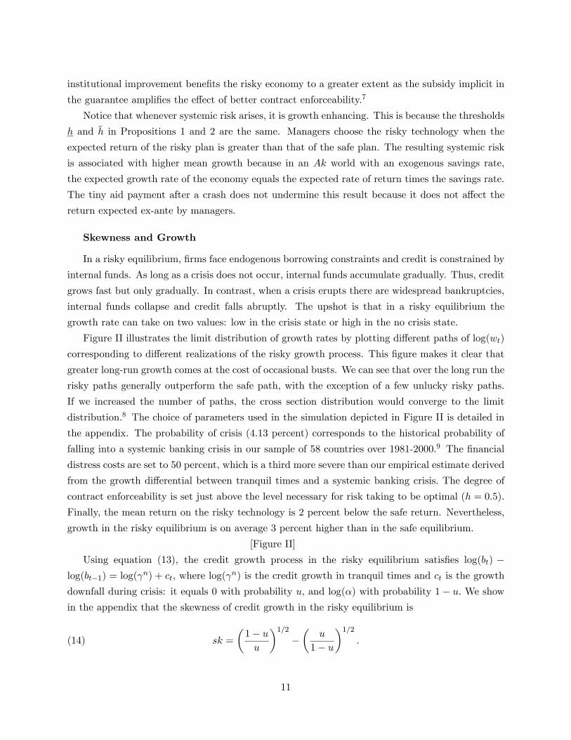
Using equation (13), the credit growth process in the risky equilibrium satis�es log(bt) �log(bt�1) = log( n) + ct; where log( n) is the credit growth in tranquil times and ct is the growth
downfall during crisis: it equals 0 with probability u; and log(�) with probability 1� u: We showin the appendix that the skewness of credit growth in the risky equilibrium is
(14) sk =
�1� uu
�1=2��
u
1� u
�1=2:
11
We know from Proposition 1 that a risky equilibrium exists only if crises are rare events. In
particular, the probability of crisis 1 � u must be less than half. Thus, the distribution of growthrates must be negatively skewed in a risky equilibrium. In contrast, in the safe equilibrium there is
no skewness as the growth process is smooth. Since systemic risk arises in equilibrium only when
it is growth enhancing (by Proposition 2), our model predicts that there is a positive link between
mean growth and negative skewness. Since the probability of falling into a systemic banking crisis in
our sample is 4:13 percent; (14) implies that the credit growth distribution in the risky equilibrium
exhibits large negative skewness: �4:6:
Net Expected Value of Managers�Income
There are �scal costs associated with systemic risk because along a risky path bailouts must
be granted during crises, and these bailouts are �nanced by taxing �rms during good times.
Proposition 2 states that bailouts are fundable, but is the expected present value of managers�
income net of taxes greater along a risky path than along a safe path? To address this question
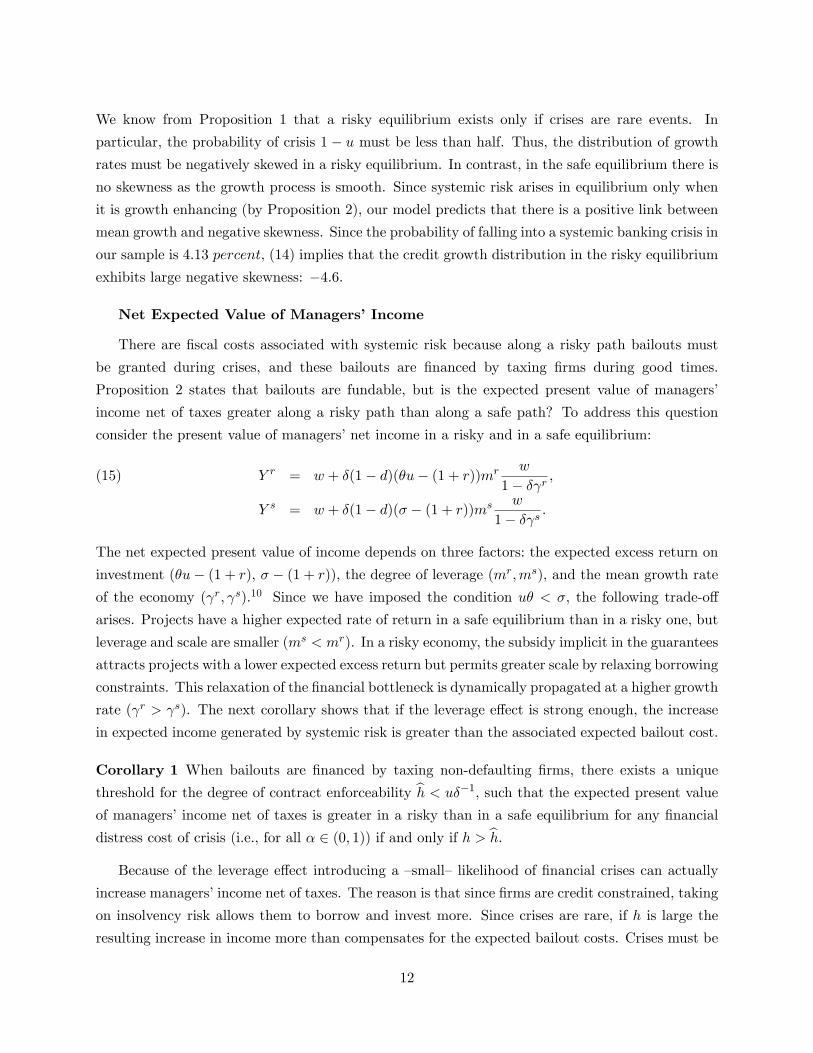
consider the present value of managers�net income in a risky and in a safe equilibrium:
Y r = w + �(1� d)(�u� (1 + r))mr w
1� � r ;(15)
Y s = w + �(1� d)(� � (1 + r))ms w
1� � s :
The net expected present value of income depends on three factors: the expected excess return on
investment (�u� (1 + r); � � (1 + r)), the degree of leverage (mr;ms), and the mean growth rate
of the economy ( r; s).10 Since we have imposed the condition u� < �; the following trade-o¤
arises. Projects have a higher expected rate of return in a safe equilibrium than in a risky one, but
leverage and scale are smaller (ms < mr). In a risky economy, the subsidy implicit in the guarantees
attracts projects with a lower expected excess return but permits greater scale by relaxing borrowing
constraints. This relaxation of the �nancial bottleneck is dynamically propagated at a higher growth
rate ( r > s). The next corollary shows that if the leverage e¤ect is strong enough, the increase
in expected income generated by systemic risk is greater than the associated expected bailout cost.
Corollary 1 When bailouts are �nanced by taxing non-defaulting �rms, there exists a unique
threshold for the degree of contract enforceability bh < u��1, such that the expected present valueof managers�income net of taxes is greater in a risky than in a safe equilibrium for any �nancial
distress cost of crisis (i.e., for all � 2 (0; 1)) if and only if h > bh:Because of the leverage e¤ect introducing a �small� likelihood of �nancial crises can actually
increase managers�income net of taxes. The reason is that since �rms are credit constrained, taking
on insolvency risk allows them to borrow and invest more. Since crises are rare, if h is large the
resulting increase in income more than compensates for the expected bailout costs. Crises must be
12

rare in order for them to occur in equilibrium. If the probability of crisis were high, agents would
not �nd it pro�table to take on risk in the �rst place. Notice that since the threshold h might be
higher than the risk taking threshold h; there may be a range (h; h) where systemic risk increases
mean growth but reduces Y:
Finally, we would like to stress that our risk-neutral setup is not designed to analyze the welfare
e¤ects of a greater propensity to crisis. For such analysis it would be more appropriate to consider
a setup with risk aversion, so that one could tradeo¤ the growth-enhancing e¤ect of systemic risk
taking against the costs of greater income uncertainty.11
II.C. Decreasing Returns Technologies
Here, we consider the case in which the production functions in (1) are concave. We show that
systemic risk may accelerate growth in a transition phase, but not inde�nitely. At some point, an
economy must switch to a safe path.
To capture the parameter restrictions in (1) we let the safe production function be proportional
to the risky one (g(I) � � � f(I)) and use the following parametrization:
(16) f(I) = I�; g(I) = � � I�; � 2 (0; 1); 0 < u < � < 1:
Since u < � < 1; the risky technology yields more than the safe technology in the good state but
has a lower expected return. This captures the same idea as u� < � < �: Meanwhile, since f(I) is
concave, the condition analogous to 1 + r < u� only holds for low levels of capital.
In order to reduce the number of cases we need to consider, we assume that at any point in time,
either the risky or the safe technology can be used but that both cannot be used simultaneously.
Also, we assume that when a majority of �rms is insolvent a bailout is granted to the lenders of
insolvent �rms that did not divert funds. The rest of the model remains the same. Under these
assumptions one can derive the following proposition, which is the analogue of Proposition 1.
Proposition 3 Borrowing constraints arise in equilibrium only if the degree of contract enforce-
ability is not too high (h < �t+1��1): If this condition holds, then:
� For all levels of w there exists a �safe�CME in which all �rms only invest in the safe technologyand a systemic crisis in the next period cannot occur: �t+1 = 1.
� There is a unique threshold for internal funds w� 2 ( ~Imr ; ~I), such that there also exists a risky
CME in which �t+1 = u if and only if w < w� and h 2 (hy; �h); where hy is de�ned in theappendix.
� In the safe and risky CME borrowing constraints bind for internal funds lower than Ims and
~Imr ; respectively. Investment is given by
13
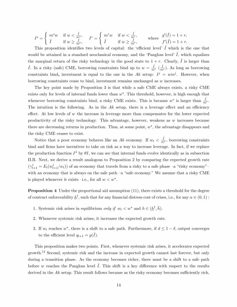
Is =
(msw if w < I
ms ;
I if w � Ims ;
Ir =
(mrw if w <
~Imr ;
~I if w � ~Imr ;
whereg0(I) = 1 + r;
f 0(~I) = 1 + r:
This proposition identi�es two levels of capital: the �e¢ cient level� I which is the one that
would be attained in a standard neoclassical economy, and the �Pangloss level� ~I; which equalizes
the marginal return of the risky technology in the good state to 1 + r. Clearly, ~I is larger than
I. In a risky (safe) CME, borrowing constraints bind up to w =~Imr (
Ims ): As long as borrowing
constraints bind, investment is equal to the one in the Ak setup: Ij = wmj . However, when
borrowing constraints cease to bind, investment remains unchanged as w increases.
The key point made by Proposition 3 is that while a safe CME always exists, a risky CME
exists only for levels of internal funds lower than w�: This threshold, however, is high enough that
whenever borrowing constraints bind, a risky CME exists. This is because w� is larger than~Imr :
The intuition is the following. As in the Ak setup, there is a leverage e¤ect and an e¢ ciency
e¤ect. At low levels of w the increase in leverage more than compensates for the lower expected
productivity of the risky technology. This advantage, however, weakens as w increases because
there are decreasing returns in production. Thus, at some point, w�; the advantage disappears and
the risky CME ceases to exist.
Notice that a poor economy behaves like an Ak economy. If wt <~Imr ; borrowing constraints
bind and �rms have incentives to take on risk as a way to increase leverage. In fact, if we replace
the production function I� by �I; we can see that internal funds evolve identically as in subsection
II.B. Next, we derive a result analogous to Proposition 2 by comparing the expected growth rate
( jt+1 = Et(wjt+1=wt)) of an economy that travels from a risky to a safe phase �a �risky economy��
with an economy that is always on the safe path �a �safe economy.�We assume that a risky CME
is played whenever it exists �i.e., for all w < w�.
Proposition 4 Under the proportional aid assumption (11), there exists a threshold for the degree
of contract enforceability hy; such that for any �nancial distress cost of crises, i.e., for any � 2 (0; 1) :
1. Systemic risk arises in equilibrium only if wt < w� and h 2 (hy; �h):
2. Whenever systemic risk arises, it increases the expected growth rate.
3. If wt reaches w�; there is a shift to a safe path. Furthermore, if d � 1� �; output convergesto the e¢ cient level qt+1 = g(I):
This proposition makes two points. First, whenever systemic risk arises, it accelerates expected
growth.12 Second, systemic risk and the increase in expected growth cannot last forever, but only
during a transition phase. As the economy becomes richer, there must be a shift to a safe path
before w reaches the Pangloss level ~I: This shift is a key di¤erence with respect to the results
derived in the Ak setup. This result follows because as the risky economy becomes su¢ ciently rich,
14

borrowing constraints cease to bind, so the leverage bene�ts due to risk taking go away. Recall that
on a risky path, borrowing constraints are binding up to w =~Imr ; which is less than w�: Finally,
we show in the proof that under the condition d � 1� �; the transition curve is always above the45-degree line in the (wt; wt+1) space. Thus, the economy will not cycle between the safe and risky
phases. Once it reaches the safe phase, it stays there forever. In this case, output converges to
g(I); and the excess of w over I is saved and thus earns the world interest rate.
III. Systemic Risk and Growth: The Empirical Link
The empirical analysis of the link between systemic risk and growth faces several challenges.
The �rst challenge is measurement. In subsection III.A, we discuss why skewness of credit growth is
a good de facto measure of systemic risk and how skewness is linked to �nancial crisis indexes. The
second challenge is the identi�cation of a channel linking systemic risk and growth. In subsection
III.B, after having established a robust and stable partial correlation between the skewness of credit
growth and GDP growth, we test an identifying restriction derived from our theoretical mechanism:
the link between skewness and growth is strongest in the set of �nancially liberalized countries with
moderately weak institutions. The third challenge is robustness. In subsection III.C, we present
an alternative analysis of the link between systemic risk and growth based on several indexes of
�nancial crises. In subsection III.D, we test a further implication of our theoretical mechanism
which is that skewness increases growth via its e¤ect on investment. Finally, subsection III.E
presents a set of additional robustness tests.
III.A. Measuring Systemic Risk
We use the skewness of real credit growth as a de facto indicator of �nancial systemic risk.
The theoretical mechanism that links systemic risk and growth implies that �nancial crises are
associated with higher mean growth only if they are rare and systemic. If the likelihood of crisis
were high, there would be no incentives to take on risk. If crises were not systemic, borrowers could
not exploit the subsidy implicit in the guarantees and increase leverage. These restrictions �rare
and systemic crises�are the conditions under which negative skewness arises. During a crisis there
is a large and abrupt downward jump in credit growth. If crises are rare, such negative outliers
tend to create a long left tail in the distribution and reduce skewness.13 When there are no other
major shocks, rare crisis countries exhibit strictly negative skewness.14
To illustrate how skewness is linked to systemic risk, the kernel distributions of credit growth
rates for India and Thailand are given in Figure III.15 India, the safe country, has a lower mean and
is quite tightly distributed around the mean, with skewness close to zero. Meanwhile, Thailand,
the risky fast-growing country, has a very asymmetric distribution with large negative skewness.
15

Negative skewness can also be caused by forces other than �nancial systemic risk. We control
explicitly for the two exogenous events that we would expect to lead to a large fall in credit: severe
wars and large deteriorations in the terms of trade. Our data set consists of all countries for which
data are available in the World Development Indicators and International Financial Statistics for
the period 1960-2000. Out this set of eighty-three countries we identify twenty-�ve as having a
severe war or a large deterioration in the terms of trade.16
Crises are typically preceded by lending booms. However, the typical boom-bust cycle generates
negative, not positive, skewness. Even though during a lending boom credit growth rates are large
and positive, the boom typically takes place for several years and in any given year is not as large
in magnitude as the typical bust.17 [Figure III]
Correspondence Between Skewness and Crisis Indexes
In principle, the sample measure of skewness can miss cases of risk taking that have not yet led to
crisis. This omission, however, makes it more di¢ cult to �nd a negative relationship between growth
and realized skewness. Thus, it does not invalidate our empirical strategy. What is important,
though, is that skewness captures mostly �nancial crises once we control for wars and large terms
of trade deteriorations. To investigate this correspondence, we consider ten standard indexes: three
of banking crises, four of currency crises and two of sudden stops.18 We then identify two types of
crises: coded crises, which are classi�ed as a crisis by any one of the indexes, and consensus crises.
The latter are meant to capture truly severe crises and are de�ned as follows: First, the episode is
identi�ed by at least two banking crises indexes or two currency crises indexes or two sudden stop
indexes. Second, it has not been going on for more than ten years, and, third, it does not exhibit
credit growth of more than 10 percent.19
First, we �nd that our skewness measure captures mostly coded crises as: (i) the elimination
of 2 (or 3) extreme negative credit growth observations suppresses most of the negative skewness;
and (ii) at least 79 percent of these extreme observations correspond to coded crises. Table I, panel
A shows that among the countries with negative skewness, 90 percent (79 percent) of the 2 (3)
extreme negative observations are coded as a crisis. Moreover, if we eliminate the 2 (3) extreme
observations, skewness increases on average from -0.7 to +0.16 (0.36), and in 79 percent (90 percent)
of the cases, skewness increases to more than -0.2, which is close to a symmetric distribution. These
are particularly high numbers given the fact that we forced each country to have 2 (3) outliers. It
remains, in theory, a possibility that skewness is a¤ected by non-extreme observations. To consider
this possibility, for each country we eliminate the three observations whose omission results in the
highest increase in skewness. Panel B in Table I shows that this procedure eliminates virtually all
negative skewness. Moreover, 79 percent of the omitted observations correspond to coded crises.20
[Table I]
Second, there is signi�cantly less negative skewness once we exclude consensus crises. Table I,
16
panel C, shows that if we eliminate the observations with a consensus crisis, skewness increases
in 32 out of the 35 crisis countries.21 On average, skewness increases from -0.41 to 0.32 and the
percentage of crisis countries with skewness below -0.2 shrinks from 63 percent to 11 percent.22
In sum, there is a fairly close correspondence between both measures. There are, however,
advantages and disadvantages to the use of both skewness and crisis indexes as proxies for systemic
risk. On the one hand, skewness simply looks for abnormal patterns in an aggregate �nancial
variable and does not use direct information about the state of the �nancial system. On the other
hand, it is objective and can be readily computed for large panels of countries over long time
periods. Furthermore, skewness signals in a parsimonious way the severity of rare credit busts. In
contrast, de jure banking crisis indexes are based on more direct information. Unfortunately, they
are subjective, limited in their coverage over countries and time, and do not provide information
on the relative severity of crises.23 Other �nancial crisis indexes �e.g., currency crisis and sudden
stops�are, like skewness, de facto indexes.24 However, the rules followed to construct these indexes
di¤er from one author to another. As a result, it is not unusual for these crisis indexes to identify
di¤erent episodes.
Finally, consider Thailand as an example to illustrate the two procedures. Figure IV, panel A
exhibits Thailand�s credit growth rates. We see two severe busts with negative growth rates (1980
and 1998-2000), and a slowdown with small positive growth rates (1985-86). Figure IV, panel
B displays the same information using histograms and kernel distributions, which are smoothed
histograms. The �rst panel covers the entire sample, in which skewness is -0.90. The second panel
eliminates the consensus crisis years: 1998-2000 and 1985-87. We see that although coded crises
indexes capture the well-known 1998-2000 crisis, they do not report the severe 1980 bust and place
the mild 1985-1986 episode on an equal footing with the severe 1998-2000 crisis episode.25 As a
result, when 1985-1987 and 1998-2000 are eliminated, skewness remains almost unchanged at -0.99.
If instead we eliminate the major negative outliers (1998-2000 and 1980), the third panel shows
that skewness shrinks abruptly to -0.196. If we also eliminate 1986, the year with the next smallest
growth rate, skewness becomes virtually zero (+0.04).
[Figure IV]
Variance and Excess Kurtosis
Rare and severe crises are associated not only with negative skewness but also with high variance
and excess kurtosis. We consider each in turn.
Variance is the typical measure of volatility. For the purpose of identifying systemic risk there
are, however, two key di¤erences between variance and skewness. First, variance re�ects not only
large and abrupt busts that occur during crises, but may also re�ect other more symmetric shocks.
In contrast, skewness captures speci�cally asymmetric and abnormal patterns in the distribution
of credit growth.26 Second, if crises were not rare but the usual state of a¤airs, unusually high
17

variance, not large negative skewness, would arise.27 Therefore, unlike variance, skewness isolates
the incidence of severe and rare crises from other sources of more frequent or more symmetric
volatility.
Our model does not make predictions on how symmetric shocks a¤ect growth.28 As we shall
show below, our regression results do not contradict the negative link between variance and growth
found by Ramey and Ramey [1995] and others.
Excess kurtosis captures both the fatness of the tails and the peakedness of a distribution
relative to those of a normal distribution.29 Positive excess kurtosis can be generated either by
extreme events or by a cluster of observations around the mean that a¤ect the peakedness of the
distribution.30 Consider the sample of 35 countries with at least one consensus crisis. For the vast
majority of countries, excess kurtosis is driven by extreme observations associated with crises. In
about one �fth of the sample, however, excess kurtosis is predominantly a¤ected by observations
near the center of the distribution. As a result, in our sample, the link between skewness and crises
is empirically stronger than the link between excess kurtosis and crises.31
III.B. Skewness and Growth
We start by presenting baseline evidence of the link between skewness and growth based on
cross-section regressions estimated by OLS, and panel regressions estimated by GLS using ten-year
non-overlapping windows. We then test the identifying restriction of our theoretical mechanism by
introducing interaction term e¤ects in the growth regressions. The sample used in the regressions
consists of the 58 countries that have experienced neither a severe war nor a large deterioration in
the terms of trade.
Baseline Estimation
In the �rst set of equations we estimate, we include the three moments of credit growth in a
standard growth equation:32
(17) �yit = 0Xit + �1��B;it + �2��B;it + �3sk�B;it + �t + "it;
where �yit is the average growth rate of per-capita GDP; ��B;it; ��B;it and sk�B;it are the mean,
standard deviation, and skewness of the growth rate of real bank credit to the private sector,
respectively; Xit is a vector of control variables; �t is a period dummy and "it is the error term.33
Here, we consider a simple control set that includes initial per-capita GDP and the initial ratio of
secondary schooling. In section III.E we show that similar results are obtained with an extended
control set that includes the simple set plus the in�ation rate, the ratio of government consumption
to GDP, a measure of trade openness and life expectancy at birth.34 We do not include investment
in (17) as we expect the three moments of credit growth, our variables of interest, to a¤ect GDP
18
growth through investment.35
We consider three sample periods: 1961-2000, 1971-2000 and 1981-2000.36 In the cross-sections,
the moments of credit growth are computed over the sample period and initial variables are mea-
sured in 1960, 1970 or 1980. In the panels, the moments of credit growth are computed over each
decade and the initial variables are measured in the �rst year of each decade.37 All panel regressions
are estimated with time e¤ects.38
Table II reports the estimation results. The novel �nding is the negative partial correlation
between the skewness of real credit growth and real GDP growth. Skewness always enters with a
negative point estimate that ranges between -0.244 and -0.334. These estimates are signi�cant at
the 5 percent level in the cross-section regressions and at the 1 percent level in the panel regressions.
The positive partial correlation between the mean of credit growth and GDP growth is standard
in the literature (e.g., Levine and Renelt [1992]). The negative partial correlation between the
standard deviation and GDP growth is consistent with the �nding of Ramey and Ramey [1995] on
the negative link between growth and variance.
[Table II]
Are these estimates economically meaningful? To address this question consider India and
Thailand over the period 1981-2000. India has near zero skewness, and Thailand a skewness of
about minus one.39 The cross-sectional estimate of -0.32 for 1981-2000 implies that a one unit
decline in skewness (from 0 to -1) is associated with a 0.32 percent increase in annual real per capita
growth. This �gure corresponds to a little less than a third of the per-capita growth di¤erential
between India and Thailand over the same period.
The negative partial correlation between skewness and growth is consistent with our model�s
prediction that a risky economy grows, on average, faster than a safe one. This is because the
former exhibits negative skewness, while the latter has no skewness. The baseline estimation
assumes an homogenous and linear e¤ect of skewness on growth. Below we relax the homogeneity
assumption and test whether the link between skewness and growth depends on the degree of
�nancial liberalization and of contract enforceability. In the robustness subsection, we relax the
linearity assumption and enter negative and positive skewness separately in the growth regression.
Identi�cation of the Mechanism
Here, we test an identi�cation restriction implied by the equilibria of our model. Namely,
whether the link between skewness and growth is stronger in the set of �nancially liberalized
countries with a medium degree of contract enforceability than in other countries.40
In the model, systemic guarantees are equally available to all countries. However, countries di¤er
crucially in their ability to exploit these guarantees by taking on systemic risk. First, an equilibrium
with systemic risk exists and is growth enhancing only in the set of �nancially liberalized countries
with a �medium�degree of contract enforceability h. On the one hand, borrowing constraints arise
19
in equilibrium only if contract enforceability problems are �severe�: h < �h so borrowers may �nd it
pro�table to divert funds. On the other hand, risk taking is individually optimal and systemic risk
is growth enhancing only if h > h: Only if h is large enough can risk taking induce enough of an
increase in leverage to compensate for the distress costs of crises. Second, the mechanism requires
not only weak institutions but also policy measures that are conducive to the emergence of systemic
risk. Financial liberalization can be viewed as such a policy measure. In non-liberalized economies,
regulations do not permit agents to take on systemic risk. Next, we exploit cross-country di¤erences
in �nancial liberalization and contract enforceability to test this identifying restriction.
We use the law and order index of the Political Risk Service Group in 1984 to construct the
set of countries with a medium degree of contract enforceability (MEC).41 We classify as MECs
the countries with an index in 1984 ranging between 2 and 5.42 We use three alternative indexes
of �nancial liberalization: First, a de facto binary index based on the identi�cation of trend breaks
in capital �ows, which is equal to one if a country is liberalized in a given year and zero otherwise.
By averaging this index over 10 years, we obtain the share of liberalized years in a given decade.
Second, the de jure index of Quinn [2001] that reports on a zero to one scale the intensity of
capital account liberalization based on the International Monetary Fund report on capital account
restrictions. Third, the de jure index of Abiad and Mody [2004]. The de facto index is computed
for the full sample of 58 countries for the period 1981-2000. The two other indexes cover fewer
countries, but are available for a longer time period.43
We generate a composite index by combining an MEC dummy �that equals one for MEC
countries and zero otherwise�with one of the liberalization indexes. For each country i and each
of our non-overlapping ten-year windows (t; t+ 9); the index equals
(18) MECi_FLi;t =MECi �1
10
9Xj=0
fli;t+j , t 2 f1961; 1971; 1981; 1991g:
For each liberalization index, we interact the MEC_FL index with the three moments of credit
growth and add them to regression equation (17).44 Table III shows that, consistent with the
restrictions imposed by the model, the e¤ect of skewness on growth is strongest among MEC_FL
countries. The interaction term skewness �MEC_FL enters negatively and signi�cantly at the1 percent level in the three regressions. Its point estimate ranges between -1.00 and -0.75. By
contrast, the coe¢ cient of skewness is not signi�cantly di¤erent from zero. It ranges between -0.08
and -0.01. The di¤erence between the two estimates indicates that the link between skewness and
growth is not only stronger in the MEC_FL set, but that it also only exists within this set.
By adding up the interacted and non-interacted skewness coe¢ cients, we obtain the e¤ect of
skewness on growth for a fully liberalized MEC country. The point estimates of this e¤ect �
reported at the bottom of Table III� range between -1.02 and -0.81 and are signi�cant at the 1
20

percent level.An estimate of -0.81 means that a one unit increase in negative skewness for a fully
liberalized MEC country is associated with a 0.81 percentage point increase in annual GDP growth.
This e¤ect is three times larger than the homogenous e¤ect estimated in Table II. [Table III]
We have shown that the negative link between skewness and growth emerges only in the set
of �nancially liberalized countries with a medium level of contract enforceability. By validating
the identifying restrictions of our theoretical mechanism, this �nding supports our hypothesis that
systemic risk is growth enhancing.
III.C. Crisis Indexes and Growth
In subsection III.A we showed that our skewness measure coincides closely with several �nancial
crisis indexes. Here we show that, for the subsamples covered by crisis indexes, the same link is
also evident when we replace skewness with crisis indexes in our growth regressions.
We consider three banking crisis indexes (Caprio-Klingebiel, Demirguc-Detragiache and a con-
sensus index), a sudden stop consensus index and a currency crisis consensus index.45 For each
crisis index we set a dummy equal to one if the country has experienced a crisis during the decade
and zero otherwise. Using a crisis dummy computed over ten years allows us to capture the aver-
age medium-run growth impact of crises rather than just the growth shortfall experienced during
a crisis.46 [Table IV]
The empirical speci�cation is the same as in the panel analysis of Table II, substituting the
crisis dummies for skewness. Table IV shows that the three banking crisis dummies enter positively
(with point estimates ranging from +0.22 to +0.26) and signi�cantly at the 5 percent level. Thus,
we �nd that countries that experienced a systemic banking crisis in a given decade also experience
on average a 0.24 percent annual increase in per-capita GDP growth. Interestingly, this e¤ect is
similar in magnitude to that of a one unit change in skewness (see Table II). Turning to the other
crisis indexes, we �nd a similar positive growth e¤ect of sudden stops, but we do not �nd any
signi�cant growth e¤ect of currency crises.47 Finally, in Table EA1, in the appendix we show that
the results of Table IV persist when the estimation is done with the full set of control variables.
III.D. Skewness and Investment
In our mechanism, systemic risk taking leads to higher mean growth because it helps relax
borrowing constraints and thus allows �rms to invest more. Although the link between investment
and growth has been extensively analyzed in the literature, the link between systemic risk and
investment has not. Here we analyze this link by adding the skewness of credit growth to a panel
investment regression. Following Barro [2001], we regress the investment-to-GDP ratio on our
controls and the lagged investment rate, which captures the high degree of serial correlation in the
investment rate. We calculate investment rates in two ways: using real PPP-converted prices and
21

using domestic prices. [Table V]
Table V, panel A presents the results of the GLS and GMM panel estimations performed over
the period 1971-2000 for the two investment rates using the simple set of control variables.48 ;49 The
estimation yields very similar results for the two investment rates. Skewness enters negatively and
is signi�cant at the 1 percent level in the GLS estimations and at the 5 percent level in the GMM
estimation. Furthermore, investment is positively correlated with the mean of credit growth and
negatively with the standard deviation. The e¤ect of skewness on investment is slightly larger in
the GMM estimation. In the GMM (GLS) estimation, a one unit increase in skewness is associated
with a 1.1 (0.77) percentage point direct e¤ect on the investment rate at domestic prices.50
In order to relate the investment e¤ects to growth outcomes, we present in Table V, panel B,
a set of growth regressions in which the investment rate replaces the moments of credit growth.
Investment enters signi�cantly at the 1 percent level with point estimates close to 0.2, a standard
value in the growth literature (e.g., Levine and Renelt [1992]). By combining the e¤ect of skewness
on investment (0.77) with the corresponding e¤ect of investment on growth (0.22), one obtains
�0:17: This �gure is of the same order of magnitude as the direct e¤ect of skewness on growthin the panel regression presented in Table II for the same sample period ( � 0:24), although it isslightly lower.51
The identi�cation of a negative link between skewness and investment and a positive link be-
tween investment and growth reinforces the support we have found for our theoretical mechanism
where systemic-risk taking a¤ects growth through an investment channel.
III.E. Robustness
Here, we summarize a series of robustness tests of the link between skewness and growth.
Generalized Method of Moments System Estimation. In order to control for unobserved time- and
country-speci�c e¤ects, and account for some endogeneity in the explanatory variables, we use a
GMM system estimator developed by Blundell and Bond [1998]. The system is estimated over the
period 1970-2000. Tables EA6 and EA7 in the appendix show that (i) the negative link between
skewness and growth is signi�cant in the GMM estimation and its point estimate is actually larger
than in the GLS estimation; (ii) relaxing the exogeneity on skewness while treating the other
regressors as jointly endogenous, has little e¤ect on the estimates; and (iii) the interaction e¤ects
presented in subsection III.B are also signi�cant in the GMM speci�cation. The details of the GMM
estimation are presented in the appendix.52
Extended Set of Control Variables. Table EA8 in the appendix presents the panel estimates
obtained with the extended control set for the three estimation periods. The coe¢ cients of the
moments of credit growth are very similar to the panel estimates obtained in Table II. Notice also
that in most of the regressions, the control variables enter with the expected sign and their point
22

estimates are signi�cant.53
Alternative MEC Sets. Table EA9 in the appendix shows the results of section III.B are robust
to alternative de�nitions of the set of countries with a medium degree of contract enforceability.
In the three regressions presented in Table EA9, we exclude successively from the MEC set: (i)
countries with an index of 2, (ii) countries with an index of 5, and (iii) countries with an index
equal to either 2 or 5. In the �rst regression, the link between skewness and growth is only present
in the MEC_FL set, while in the two other regressions, this negative link is at least three times
larger in this set.54
Negative Skewness and Growth. Table EA10 in the appendix shows that the negative link between
skewness and growth re�ects mainly a positive relationship between the magnitude of negative
skewness and growth. The magnitude of negative (positive) skewness is computed as a variable
equal to the absolute value of skewness if skewness is negative (positive) and equal to zero otherwise.
When these two variables are introduced in place of skewness in our benchmark panel estimations
(Table II, regressions 4 to 6), we �nd that (i) the magnitude of negative skewness enters positively
and signi�cantly at the one percent con�dence level, with point estimates ranging between 0.48 and
0.55; and (ii) the magnitude of positive skewness enters negatively but not signi�cantly di¤erent
from zero.
Skewness vs. Crises Indexes. In order to run a horse race between coded crisis indexes and
skewness, we add the skewness of credit growth to each of the regressions presented in Table IV.
The results are presented in Table EA11 of the appendix. The skewness coe¢ cients are signi�cant
and their point estimates are only slightly lower than the coe¢ cient estimated in the baseline
regression (Table II, regression 6). In contrast, the coe¢ cients of systemic banking crises indexes
and the coe¢ cient of the sudden stops index lose their signi�cance, and their point estimate fall
sharply once skewness is introduced.
The Full Sample of Countries. In order to interpret the link between skewness and growth as the
result of endogenous systemic risk taking, in our benchmark estimation we have controlled for two
other main sources of skewness: war and large terms-of-trade shocks. These shocks are exogenous
and we do not expect them to re�ect the relaxation of �nancial bottlenecks induced by systemic
risk taking. Nevertheless, to investigate whether the negative link between skewness and growth
is observed in an unconditional sample, we re-estimate the panel regression presented in Table II
including the full sample of 83 countries for which we have available data. Table EA12 shows that
skewness still enters negatively and remains statistically signi�cant at the 1 percent level, although
the magnitude of the average point estimate is reduced from -0.29 to -0.22.
Outliers. To test whether the link between skewness and growth may be driven by outliers, we
consider the GLS panel regression performed with the simple control set over 1961-2000 (regression
23

4, Table II). There are 13 country-decades whose residuals deviate by more than two standard
deviations from the mean.55 As Table EA13 shows, the exclusion of outliers does not change
our results. In particular, the coe¢ cient on skewness ranges between -0.30 and -0.35, excluding
individual outliers, and is -0.24 when all outliers are excluded. These estimates are signi�cant at
the one percent con�dence level and are quite similar to our benchmark estimate of -0.33.
IV. Related Literature
A novelty of this paper is to use skewness to analyze economic growth. In the �nance literature,
skewness has been used to capture asymmetry in risk in order to explain the cross-sectional varia-
tion of excess returns. If, holding mean and variance constant, investors prefer positively skewed to
negatively skewed portfolios, the latter should exhibit higher expected returns. Kraus and Litzen-
berger [1976] show that adding skewness to the CAPM model improves its empirical �t. Harvey and
Siddique [2000] �nd that coskewness has a robust and economically important impact on equity
risk-premia even when factors based on size and book-to-market are controlled for.56 Veldkamp
[2005] rationalizes the existence of skewness in assets markets in a model with endogenous �ows
of informations. In the macroeconomic literature, Barro [2006] measures the frequency and size of
large GDP drops over the twentieth century and shows that these rare disasters can explain the
equity premium puzzle.
In our empirical analysis, the negative link between skewness and growth coexists with the
negative link between variance and growth identi�ed by Ramey and Ramey [1995], Fatas and
Mihov [2003] and others. The contrasting growth e¤ects of di¤erent sources of risk are also present
in Imbs [2004], who �nds that aggregate volatility is bad for growth, while sectoral volatility is
good for growth.
Most of the empirical literature on �nancial liberalization and economic performance focuses
either on growth or on �nancial fragility and excess volatility. On the one hand, Bekaert, Harvey and
Lundblad [2005] �nd a robust and economically important link between stock market liberalization
and growth; Henry [2002] �nds similar evidence by focusing on private investment; while Klein
[2005] �nds that �nancial liberalization is growth enhancing only among middle-income countries.
On the other hand, Kaminsky and Reinhart [1998] and Kaminsky and Schmukler [2002] show
that the propensity to crisis and stock market volatility increase in the aftermath of �nancial
liberalization. Our �ndings help to integrate these contrasting views.
Obstfeld [1994] demonstrates that �nancial openness increases growth if international risk-
sharing allows agents to shift from safe to risky projects with a higher return. In our framework,
risky projects have a lower expected return than safe ones. The growth gains are obtained because
�rms that take on more risk can attain greater leverage.
In our paper, liberalization policies that discourage hedging can induce higher growth because
24

they help ease borrowing constraints. Tirole and Pathak [2006] reach a similar conclusion in a
di¤erent setup. In their framework, a country pegs the exchange rate as a means to signal a strong
currency and attract foreign capital. Thus, it must discourage hedging and withstand speculative
attacks in order for the signal to be credible.
By focusing on the growth consequences of imperfect contract enforceability, this paper is con-
nected with the growth and institutions literature. For instance, Acemoglu et. al. [2003] show that
better institutions lead to higher growth, lower variance and less frequent crises. In our model,
better institutions also lead to higher growth, and it is never optimal for countries with strong
institutions to undertake systemic risk. Our contribution is to show how systemic risk can enhance
growth by counteracting the �nancial bottlenecks generated by weak institutions.
The cycles in this paper are di¤erent from schumpeterian cycles in which the adoption of new
technologies and the cleansing e¤ect of recessions play a key role. Our cycles resemble Juglar�s credit
cycles in which �nancial bottlenecks play a dominant role. Juglar (1862) characterized asymmetric
credit cycles along with the periodic occurrence of crises in France, England, and the United States
during the nineteenth century.
V. Conclusions
Our �nding that fast growing countries tend to experience occasional crises sheds light on two
contrasting views of �nancial liberalization. In one view, �nancial liberalization induces excessive
risk taking, increases macroeconomic volatility and leads to more frequent crises. In another view,
liberalization strengthens �nancial development and contributes to higher long-run growth. Our
�ndings indicate that, while liberalization does lead to systemic risk taking and occasional crises,
it also raises growth rates, even when the costs of crises are taken into account.
In order to uncover the link between systemic risk and growth, it is essential to distinguish
between booms punctuated by rare, abrupt busts and up-and-down patterns that are more frequent
or more symmetric. While both of these patterns will increase variance, only the former causes a
decline in skewness. This is why we use the skewness of credit growth, not variance, to capture
the volatility generated by crises. An innovation in this paper is the use of skewness as a de facto
indicator of �nancial systemic risk in order to study economic growth.
We analyze the relationship between systemic risk and growth by developing a theoretical
mechanism based on the existence of �nancial bottlenecks. In countries with institutions that are
weak �but not too weak, �nancial liberalization may give rise to systemic risk, enabling �nancially
constrained �rms to attain greater leverage and to increase investment and growth along a path
without crises. This is the leverage e¤ect. We show that in the set of �nancially liberalized countries
with moderate institutional problems, the leverage e¤ect is strong enough that the gains from larger
investment will dominate the losses from occasional �nancial crises.
25

The data strongly supports the empirical hypotheses associated with these theoretical results:
over the last four decades, the link between skewness and growth is strongest in �nancially liber-
alized countries with a moderate degree of contract enforceability. Furthermore, investment is the
main channel through which skewness a¤ects growth.
We would like to emphasize that the fact that systemic-risk can be good for growth does not
mean that it is necessarily good for welfare. Furthermore, as the decreasing returns version of
the model demonstrates, systemic risk taking is not a strategy for increasing growth that can be
pursued in the very long-run. Once a country becomes rich enough, it must shift to a safe path.
Finally, within the model there are several policies that could increase investment without
incurring crisis costs. A major improvement in the contract enforceability environment eliminates
�nancial bottlenecks. However, it often takes a long time for this institutional reform to be achieved.
An alternative policy is to grant failure-unrelated subsidies to �rms. However, in the real world,
such a policy might lead to cronyism and rampant corruption.
International Monetary Fund Research Department
University of California Los Angeles and N.B.E.R.
University of Osnabruck and CESifo
References
[1] Abiad, Abdul, and Ashoka Mody, �Financial Reform: What Shakes it? What Shapes it?�
American Economic Review, XCV (2005), 66-88.
[2] Acemoglu, Daron, Simon Johnson, James Robinson, and Yunyong Thaicharoen, �Institutional
Causes, Macroeconomic Symptoms: Volatility, Crises and Growth,�Journal of Monetary Eco-
nomics, L (2003), 49-103.
[3] Aghion, Philippe, Philippe Bacchetta, Romain Ranciere, and Kenneth Rogo¤, �Exchange Rate
Volatility and Productivity Growth: The Role of Financial Development,� NBER Working
Paper 12117, 2006.
[4] Barlevy, Gadi, �The Cost of Business Cycles under Endogenous Growth,�American Economic
Review, XCIV (2004), 964-990.
[5] Barro, Robert J., �Economic Growth in East Asia Before and After the Financial Crisis,�
NBER Working Paper 8330, 2001.
[6] ________, �Rare Disasters and Asset Markets in the Twentieth Century,�Quarterly Jour-
nal of Economics, CXXI (2006), 823-866.
26
[7] ________, �On the Welfare Costs of Consumption Uncertainty,�Mimeo, Harvard Univer-
sity, 2007.
[8] Bekaert, Geert, Campbell R. Harvey, and Christian Lundblad, �Does Financial Liberalization
Spur Growth?�Journal of Financial Economics, LXXVII (2005), 3-56.
[9] Bernanke, Ben S., Mark Gertler, and Simon G. Gilchrist, �The Financial Accelerator in a
Quantitative Business Cycle Framework,�in John B. Taylor and Michael Woodford eds., Hand-
book of Macroeconomics (Amsterdam: North-Holland, 1999).
[10] Blundell, Richard, and Stephen Bond, �Initial Conditions and Moment Conditions in Dynamic
Panel Data Models,�Journal of Econometrics, LXXXVII (1998), 115-143.
[11] Fatás, Antonio, and Ilian Mihov, �The Case For Restricting Fiscal Policy Discretion,�The
Quarterly Journal of Economics, CXVIII (2003), 1419-1447.
[12] Harvey, Campbell R., and Akhtar R. Siddique, �Conditional Skewness in Asset Pricing,�The
Journal of Finance, LV (2000), 1263-1295.
[13] Hauk, William R., and Romain Wacziarg, �A Monte Carlo Study of Growth Regressions,�
NBER Technical Working Paper 0296, 2004.
[14] Henry, Peter Blair, �Do Stock Market Liberalizations Cause Investment Booms,�Journal of
Financial Economics, LVIII (2002), 301-334.
[15] Imbs, Jean, �Growth and Volatility,�Journal of Monetary Economics, 2004, forthcoming.
[16] Juglar, Clément, Des Crises Commerciales et Leur Retour Periodique en France, en Angleterre
et aux Etats-Unis (Paris: Guillaumin, 1862).
[17] Kaminsky, Graciela L., and Carmen Reinhart, �The Twin Crises: The Causes of Banking and
Balance of Payments Problems,�The American Economic Review, LXXXIX (1999), 473-500.
[18] ________, and Sergio Schmukler, �Short-Run Pain, Long-Run Gain: The E¤ects of Fi-
nancial Liberalization,�Mimeo, The Worldbank, 2002.
[19] Kiyotaki, Nobuhiro, and John Moore, �Credit Cycles,�The Journal of Political Economy, CV
(1997), 211-248.
[20] Klein, Michael W., �Capital Account Liberalization, Institutional Quality and Economic
Growth: Theory and Evidence,�NBER Working Paper 11112, 2005.
[21] Kotz, Samuel, and Norman L. Johnson, �Kurtosis,�Encyclopedia of Statistical Sciences (New
York: John Wiley & Sons, 1983).
27
[22] Kraus, Alan, and Robert H. Litzenberger, �Skewness Preference and the Valuation of Risky
Assets,�The Journal of Finance, XXXI (1976), 1085-1100.
[23] Levine, Ross, Norman Loayza, and Thorsten Beck, �Financial Intermediation and Growth:
Causality and Causes,�Journal of Monetary Economics, XLVI (2000), 31-77.
[24] ________, and David Renelt, �A Sensitivity Analysis of Cross-Country Growth Regres-
sions,�American Economic Review, LXXXII (1992), 942-963.
[25] Obstfeld, Maurice, �Risk-Taking, Globalization, and Growth,�American Economic Review,
LXXXIV (1994), 1310-1329.
[26] Quinn, Dennis, �The Correlated Changes in International Financial Regulation,� Americal
Political Science Review, XCI (1997), 531-551.
[27] Rajan, Raghuram G., and Luigi Zingales, �Financial Dependence and Growth,� American
Economic Review, LXXXVIII (1998), 559-586.
[28] Ramey, Garey, and Valerie A. Ramey, �Cross-Country Evidence on the Link between Volatility
and Growth,�American Economic Review, LXXXV (1995), 1138-1151.
[29] Ranciere, Romain, Aaron Tornell, and Frank Westermann, �Crises and Growth: A Re-
evaluation,�NBER Working Paper 10073, 2003.
[30] Schneider, Martin, and Aaron Tornell, �Balance Sheet E¤ects, Bailout Guarantees and Finan-
cial Crises,�The Review of Economic Studies, LXXI (2004), 883-913.
[31] ________, �Concentrated Ownership and Bailout Guarantees,�Mimeo, New York Uni-
versity, 2005.
[32] Tirole, Jean, and Parag A. Pathak, �Pegs, Risk Management, and Financial Crises,� IDEI
Working Paper 438 , 2006.
[33] Tornell, Aaron, and Frank Westermann, �Boom-Bust Cycles: Facts and Explanation,� Inter-
national Monetary Fund Sta¤ Papers, XLIX (2002), 111-155.
[34] Veldkamp, Laura, �Slow Boom, Sudden Crash,�Journal of Economic Theory, CXXIV (2005),
230-257.
28

Notes
1Since we will focus on symmetric equilibria, we will not distinguish individual from aggregate variables.
2The aid payment is necessary to restart the economy in the wake of a systemic crisis.
3 In other words, because higher average growth derives from an increase in borrowing ability due to the
undertaking of systemic risk, the mechanism does not depend on the existence of a �mean-variance�channel.
That is, the mechanism does not require that high variance technologies have a higher expected return than
low variance technologies.
4This is a standard result in the macroeconomics literature on credit market imperfections, e.g. Bernanke
et. al. [2000] and Kiyotaki and Moore [1997].
5Taxes in our current setup do not distort the incentives to divert income. In the proof of Proposition 1,
we also consider an extension with a distortionary setup where old managers of solvent non-diverting �rms are
taxed, but those of diverting �rms are not taxed. We �nd that the equilibria of Proposition 1 exist provided
�old < dh=u� and u is large enough.
6Although expected pro�ts are greater in the risky than in the safe equilibrium, it does not follow that the
risky equilibrium must be played every period. Proposition 2 simply compares situations where a safe equilibrium
is played every period with situations where a risky equilibrium is played every period.
7Needless to say, the �rst best is to improve �nancial institutions dramatically, so that h exceeds �h and
borrowing constraints are no longer binding. However, we are considering economies where such institutional
changes may not be possible in the medium-run.
8 If instead of (11), the aid payment were a constant, the result in Proposition 2 illustrated in Figure II would
have to be quali�ed. This is because over time it would become more and more unlikely that the level of output
along the risky path overtakes the safe one as along a safe path w grows without bound, while along a risky
path crises would reset w to a constant with probability 1� u:9Notice that this is the probability of shifting from a non-crisis state to a crisis state, which is di¤erent from
the share of years spent in a crisis state. The probability of falling into a crisis is given by �11��2 ; where �1 is the
unconditional probability that a crisis starts in a given year, and �2 is the unconditional probability of being
in a crisis in given year.
10The sums Y r and Y s converge if and only if the manager�s payout rate d is greater than d de�ned in the
appendix.
11Barro (2007) considers a rare disasters setup and shows that, in the presence of risk aversion, changes in
the probability of disaster have major implications for welfare.
12This follows because the thresholds for wt and h are the same as those in Proposition 3. The intuition is
the same as in Proposition 2.
13Skewness is a measure of the degree of asymmetry of a distribution and is computed as sk = 1n
Xn
i=1
(yi�y)3
var3=2;
where �y is the mean and var is the variance. If the left tail is more pronounced that the right tail, the distribution
is said to have negative skewness. If the reverse is true, it has positive skewness.
14We use the skewness of real credit rather than GDP growth because the former re�ects more accurately
the e¤ects of crisis on credit constrained �rms. In middle-income countries, there is a pronounced sectoral
asymmetry in the response to crisis: while large export oriented �rms expand due to the real depreciation,
29
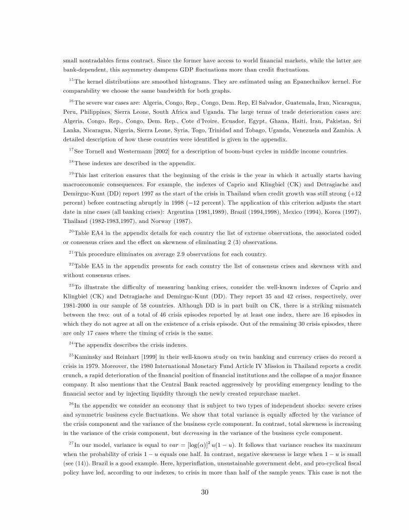
small nontradables �rms contract. Since the former have access to world �nancial markets, while the latter are
bank-dependent, this asymmetry dampens GDP �uctuations more than credit �uctuations.
15The kernel distributions are smoothed histograms. They are estimated using an Epanechnikov kernel. For
comparability we choose the same bandwidth for both graphs.
16The severe war cases are: Algeria, Congo, Rep., Congo, Dem. Rep, El Salvador, Guatemala, Iran, Nicaragua,
Peru, Philippines, Sierra Leone, South Africa and Uganda. The large terms of trade deterioration cases are:
Algeria, Congo, Rep., Congo, Dem. Rep., Cote d�Ivoire, Ecuador, Egypt, Ghana, Haiti, Iran, Pakistan, Sri
Lanka, Nicaragua, Nigeria, Sierra Leone, Syria, Togo, Trinidad and Tobago, Uganda, Venezuela and Zambia. A
detailed description of how these countries were identi�ed is given in the appendix.
17See Tornell and Westermann [2002] for a description of boom-bust cycles in middle income countries.
18These indexes are described in the appendix.
19This last criterion ensures that the beginning of the crisis is the year in which it actually starts having
macroeconomic consequences. For example, the indexes of Caprio and Klingbiel (CK) and Detragiache and
Demirguc-Kunt (DD) report 1997 as the start of the crisis in Thailand when credit growth was still strong (+12
percent) before contracting abruptly in 1998 (�12 percent): The application of this criterion adjusts the startdate in nine cases (all banking crises): Argentina (1981,1989), Brazil (1994,1998), Mexico (1994), Korea (1997),
Thailand (1982-1983,1997), and Norway (1987).
20Table EA4 in the appendix details for each country the list of extreme observations, the associated coded
or consensus crises and the e¤ect on skewness of eliminating 2 (3) observations.
21This procedure eliminates on average 2.9 observations for each country.
22Table EA5 in the appendix presents for each country the list of consensus crises and skewness with and
without consensus crises.
23To illustrate the di¢ culty of measuring banking crises, consider the well-known indexes of Caprio and
Klingbiel (CK) and Detragiache and Demirguc-Kunt (DD). They report 35 and 42 crises, respectively, over
1981-2000 in our sample of 58 countries. Although DD is in part built on CK, there is a striking mismatch
between the two: out of a total of 46 crisis episodes reported by at least one index, there are 16 episodes in
which they do not agree at all on the existence of a crisis episode. Out of the remaining 30 crisis episodes, there
are only 17 cases where the timing of crisis is the same.
24The appendix describes the crisis indexes.
25Kaminsky and Reinhart [1999] in their well-known study on twin banking and currency crises do record a
crisis in 1979. Moreover, the 1980 International Monetary Fund Article IV Mission in Thailand reports a credit
crunch, a rapid deterioration of the �nancial position of �nancial institutions and the collapse of a major �nance
company. It also mentions that the Central Bank reacted aggressively by providing emergency lending to the
�nancial sector and by injecting liquidity through the newly created repurchase market.
26 In the appendix we consider an economy that is subject to two types of independent shocks: severe crises
and symmetric business cycle �uctuations. We show that total variance is equally a¤ected by the variance of
the crisis component and the variance of the business cycle component. In contrast, total skewness is increasing
in the variance of the crisis component, but decreasing in the variance of the business cycle component.
27 In our model, variance is equal to var = [log(�)]2 u(1 � u). It follows that variance reaches its maximumwhen the probability of crisis 1� u equals one half. In contrast, negative skewness is large when 1� u is small(see (14)). Brazil is a good example. Here, hyperin�ation, unsustainable government debt, and pro-cyclical �scal
policy have led, according to our indexes, to crisis in more than half of the sample years. This case is not the
30

standard in our sample, as in most countries crises are rare. Across the �nancially liberalized countries in our
sample only 9 percent of country-years are coded as having a consensus crisis by the ten indexes we consider.
28See Barlevy [2004] for an example of an Ak model in which symmetric �uctuations reduce long-run growth
because of adjustment costs in the installation of capital.
29Excess kurtosis is computed as ek = 1n
Xn
i=1
(yi�y)4var2
� 3; where �y is the mean and �ar is the variance. Weshow in the appendix that in the risky equilibrium of the model, excess kurtosis of credit growth is 1
u(1�u) � 6;which is positive and large when crises are rare.
30According to Kotz and Johnson [1983], excess kurtosis indicates �an excess of values in the neighborhood
of the mean, as well as far away from it.� (p. 424). To illustrate this point, in the appendix we present a
theoretical example in which excess kurtosis can be created by adding mass either at the mean or at the tails
of a Normal distribution.
31The details of this analysis are included in the appendix.
32The complete description of the variables used in the regression analysis is presented in the appendix.
33 In cross-section regressions, �t is a constant, and in panel regressions it corresponds to time e¤ects.
34These control variables are standard in the empirical growth literature, e.g. Levine, Loayza and Beck [2000].
35 In section III.D, we analyze the link between investment and the three moments of credit growth.
36By using three sample periods, we make the baseline estimation results presented in this section comparable
to the results of all the regressions presented in this paper.
37For example, if the sample period is 1981-2000, two sets of moments of credit growth are computed (over
1981-1990 and 1991-2000) and the initial variables are measured in 1980 and 1990. To compute the moments
of credit growth, we impose a minimum of 8 annual observations over each non-overlapping ten-year window.
38We do not include �xed-e¤ects in our baseline regressions. The GMM estimation presented in the robustness
section is the standard method to deal with the presence of country �xed e¤ects in a dynamic equation. Moreover,
Hauk and Wacziarg [2004] have shown, using Monte-Carlo simulations, that, in the presence of measurement
error, the typical growth regression can be better estimated with the simple pooled estimators used in this
section. When within group estimators are used, they exacerbate measurement error problems.
39A one unit increase in skewness also corresponds to the average change resulting from eliminating, for each
country, the three lowest observations in the set of countries with negative skewness. See Table I.
40A similar empirical strategy is followed by Rajan and Zingales [1998] to analyze the e¤ect of �nancial
development on growth.
41This index rates countries on a 1 to 6 scale according to the quality of enforceability of the legal system.
We use the index in 1984 as it is the earliest available date. For a small number of countries for which the index
is not available in 1984, we use 1985 instead.
42Table EA9 in the appendix shows that our estimation results are robust to alternative de�nitions of the
MEC set.
43See the appendix for a detailed description of the three �nancial liberalization indexes.
44For each regression, the estimation period corresponds to the time coverage of the liberalization index.
45As described before, consensus indexes are designed to capture systemic crisis events. For each crisis type,
they record episodes that are con�rmed by at least two indexes.
31

46Using panel regression with �ve-year windows, Barro [2001] �nds that a negative contemporaneous link
between crisis and growth can coexist with a positive link when the same crisis dummy is lagged by one
�ve-year interval.
47Aghion, Bachetta, Rogo¤ and Ranciere [2006] also �nd that, on average, there is no signi�cant growth e¤ect
associated with exchange rate regime collapses.
48The speci�cation with lagged investment prevents us from estimating the investment regression over 1960-
2000. In Table EA2 in the appendix, we present similar results obtained with the extended set of control
variables.
49The GMM estimation is performed using the GMM system estimator proposed by Blundell and Bond [1998].
The details of the estimation technique are presented in the appendix.
50This number amounts to a long run e¤ect of 2.9 (2.7) percentage points, given the dynamic nature of
the investment regression. This long run e¤ect is computed as �1�� with � the skewness coe¢ cient and � the
coe¢ cient of the lagged investment rate.
51Note that by combining the two coe¢ cients, we only consider the direct e¤ect of skewness on investment and
ignore the additional dynamic e¤ect stemming from the persistence in the investment rate. More importantly,
this �gure (�0:17) is not an estimate of the indirect e¤ect of skewness on growth through an investment channel.Such an estimation would require us to estimate jointly a growth and an investment equation in a dynamic
set-up and goes beyond the purpose of this section.
52Table EA3 in the appendix shows that similar results are obtained with a three stage least squares estimation
procedure.
53An exception is initial secondary schooling that is only signi�cant with the simple set of controls.
54The signi�cant link between skewness and growth outside the MEC_FL set is the consequence of having
a more restrictive de�nition of the MEC set: it excludes some countries for which the systemic risk-taking
mechanism may be at play.
55The 13 outliers are: Bolivia (sixties), Niger (seventies and eighties), Senegal (seventies), Jordan (eight-
ies), Papua New Guinea (eighties), Brazil (seventies), Indonesia seventies), Singapore (seventies), Bostwana
(eighties), Korea (eighties), Japan (sixties) and China (nineties).
56Coskewness is the component of an asset�s skewness that is related to the skewness of the market portfolio.
32

Complete credit growth distributions
Observations eliminated Percentage of crisis years Average skewness Average skewness Share of countries with skewness >-0.2
Share of countries with skewness >0 or reduced by 80% in absolute value
2 90% -0.70 0.16 79% 65%3 79% -0.70 0.36 90% 87%
Source: Table EA4 in the appendix.
Complete credit growth distributions
Observations eliminated Percentage of crisis years Average skewness Average skewness Share of countries with skewness >-0.2
Share of countries with skewness>0 or reduced by 80% in absolute value
2 75% -0.70 0.22 86% 72%3 79% -0.70 0.45 97% 97%
Number of countries with increased skewness after elimination of crisis years
Complete distributions32 -0.41
Source: Table EA5 in the appendix.
0.32
Table ISkewness, Crises and Extreme Observations
Panel B: Observations with highest impact on skewness, coded crises and skewness
Panel A: Extreme observations, coded crises and skewnessSample: 29 countries with negative skewness (1981-2000)
Panel C: Consensus crisis years and skewnessSample: 35 countries with at least one consensus crisis (1981-2000)
Note: Panel C assesses whether the exclusion of crises increases skewness. For each country we exclude consensus crises and compute the effect on skewness. Average skewness figures correspond to cross-country averages across the sample of 35 countries with at least one consensus crisis. Consensus crises are meant to capture truly severe crises. They are defined in subsection III.A. The sample period is 1981-2000.
Note: Panel B considers the possibility that negative skewness can also be affected by non-extreme credit growth observations. We look at the countries with negative skewness, and for each country we eliminate the 2 (3) observations whose joint omission results in the highest increase in skewness. The sample period is 1981-2000.
Lowest extreme observations
Observations with highest impact on skewness Credit growth distribution without observations with highest impact on skewness
Credit growth distributions without extreme observations
Note: Panel A assesses whether extreme credit growth observations drive negative skewness. We consider the countries with negative skewness, and for each country we eliminate the 2 (or 3) lowest credit growth observations. We then compute the effect of these extreme observations on skewness and determine whether they are coded as a crisis by any of the ten crisis indexes we list in the appendix. Average skewness figures correspond to cross-country averages across the sample of 29 countries with negative skewness. The sample period is 1981-2000.
Sample: 29 countries with negative skewness (1981-2000)
Average skewness of credit growth
Distributions without crisis years

Estimation period 1961-2000 1971-2000 1981-2000 1961-2000 1971-2000 1981-2000Estimation techniqueUnit of observations
[1] [2] [3] [4] [5] [6]Moments of real credit growth:Real credit growth - mean 0.339 *** 0.348 *** 0.313 *** 0.156 *** 0.149 *** 0.159 ***
0.05 0.056 0.053 0.011 0.011 0.012Real credit growth - standard deviation -0.032 -0.068 ** -0.071 ** -0.049 *** -0.064 *** -0.048 ***
0.024 0.03 0.029 0.01 0.009 0.009Real credit growth - skewness -0.274 ** -0.334 ** -0.315 ** -0.333 *** -0.244 *** -0.268 ***
0.129 0.131 0.143 0.073 0.075 0.071
Control variables:Initial secondary schooling 0.031 ** 0.024 * 0.019 0.016 *** 0.021 *** 0.026 ***
0.013 0.013 0.018 0.004 0.004 0.003Initial income per capita -0.222 -0.283 -0.344 -0.022 -0.182 * -0.209 *** (in logs) 0.247 0.273 0.348 0.093 0.095 0.062
No. countries / No. observations 58/58 58/58 58/58 58/209 58/166 58/114
* significant at 10%; ** significant at 5%; *** significant at 1%
Note: Regressions 1 to 3 are cross-section regressions estimated by Ordinary Least Squares (OLS). Heteroskedasticity robust standard errors are reported. Regressions 4 to 6 are panel regressions estimated by Feasible Generalized Least Squares (FGLS). All the FGLS specifications include time effects. Coefficients for period dummies are not reported.
Cross-section Non-overlapping 10 year windowsOLS FGLS
Table IISkewness and Growth: Baseline Estimations
Dependent variable: Real per capita GDP growth(Standard errors are presented below the corresponding coefficient.)

Estimation period 1981-2000 1961-2000 1971-2000Unit of observationsFinancial liberalization indicator De facto De jure (Quinn) De jure (Mody)
[1] [2] [3]Moment of credit growth:Real credit growth - mean 0.105 *** 0.091 *** 0.091 ***
0.018 0.025 0.033Real credit growth - standard deviation -0.058 *** -0.077 *** -0.098 ***
0.009 0.014 0.016Real credit growth - skewness -0.011 -0.081 -0.019
0.085 0.109 0.133
Moment of credit growth interacted:Mean credit growth * MEC_FL 0.131 *** 0.170 *** 0.151 ***
0.034 0.044 0.055Standard deviation of credit growth * MEC_FL 0.047 ** 0.020 0.043
0.018 0.028 0.030Skewness of credit growth * MEC_FL -0.802 *** -0.750 *** -1.002 ***
0.165 0.244 0.275
MEC_FL -0.145 -0.026 -0.048(Medium contract enforceability*financial liberalization) 0.230 0.376 0.412
Control variables:Initial secondary schooling 0.019 *** 0.013 *** 0.000
0.006 0.005 0.008Initial income per capita -0.236 * -0.164 -0.074 (in logs) 0.140 0.123 0.152
Skewness (fully liberalized MEC countries; MEC_FL=1):Coefficient -0.810 -1.020 -0.850Standard error 0.120 0.040 0.210F-test Ho: Coefficient=0 (P-value) 0.000 0.000 0.000
No. countries / No. observations 58/114 49/163 32/96
* significant at 10%; ** significant at 5%; *** significant at 1%
Non-overlapping 10 year windows
Note: See Section III.B for the construction of the composite index of medium enforceability of contracts and financial liberalization (MEC_FL). Coefficients for period dummies are not reported.
Table IIISkewness and Growth: Country Grouping Estimations
Dependent variable: Real per capita GDP growthEstimation: Panel feasible GLS
(Standard errors are presented below the corresponding coefficient.)
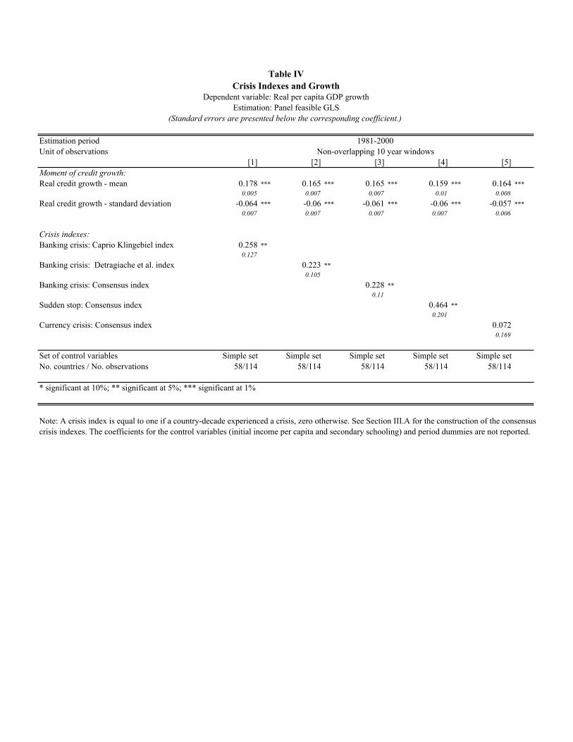
Estimation periodUnit of observations
[1] [2] [3] [4] [5]Moment of credit growth:Real credit growth - mean 0.178 *** 0.165 *** 0.165 *** 0.159 *** 0.164 ***
0.005 0.007 0.007 0.01 0.008Real credit growth - standard deviation -0.064 *** -0.06 *** -0.061 *** -0.06 *** -0.057 ***
0.007 0.007 0.007 0.007 0.006
Crisis indexes:Banking crisis: Caprio Klingebiel index 0.258 **
0.127Banking crisis: Detragiache et al. index 0.223 **
0.105Banking crisis: Consensus index 0.228 **
0.11Sudden stop: Consensus index 0.464 **
0.201Currency crisis: Consensus index 0.072
0.169
Set of control variables Simple set Simple set Simple set Simple set Simple setNo. countries / No. observations 58/114 58/114 58/114 58/114 58/114
* significant at 10%; ** significant at 5%; *** significant at 1%
1981-2000
Note: A crisis index is equal to one if a country-decade experienced a crisis, zero otherwise. See Section III.A for the construction of the consensus crisis indexes. The coefficients for the control variables (initial income per capita and secondary schooling) and period dummies are not reported.
Non-overlapping 10 year windows
Table IVCrisis Indexes and Growth
Dependent variable: Real per capita GDP growthEstimation: Panel feasible GLS
(Standard errors are presented below the corresponding coefficient.)
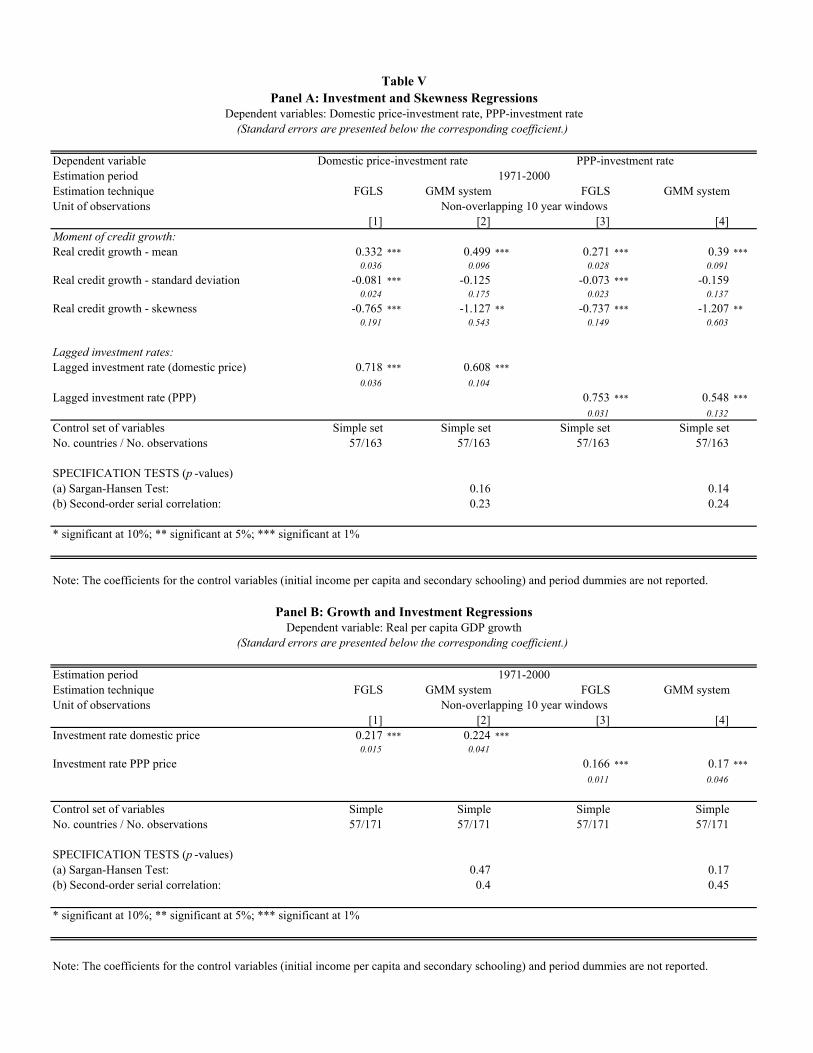
Dependent variable Estimation periodEstimation technique FGLS GMM system FGLS GMM systemUnit of observations
[1] [2] [3] [4] Moment of credit growth:Real credit growth - mean 0.332 *** 0.499 *** 0.271 *** 0.39 ***
0.036 0.096 0.028 0.091Real credit growth - standard deviation -0.081 *** -0.125 -0.073 *** -0.159
0.024 0.175 0.023 0.137Real credit growth - skewness -0.765 *** -1.127 ** -0.737 *** -1.207 **
0.191 0.543 0.149 0.603
Lagged investment rates:Lagged investment rate (domestic price) 0.718 *** 0.608 ***
0.036 0.104Lagged investment rate (PPP) 0.753 *** 0.548 ***
0.031 0.132Control set of variables Simple set Simple set Simple set Simple setNo. countries / No. observations 57/163 57/163 57/163 57/163
SPECIFICATION TESTS (p -values)(a) Sargan-Hansen Test: 0.16 0.14(b) Second-order serial correlation: 0.23 0.24
* significant at 10%; ** significant at 5%; *** significant at 1%
Estimation periodEstimation technique FGLS GMM system FGLS GMM systemUnit of observations
[1] [2] [3] [4] Investment rate domestic price 0.217 *** 0.224 ***
0.015 0.041Investment rate PPP price 0.166 *** 0.17 ***
0.011 0.046
Control set of variables Simple Simple Simple SimpleNo. countries / No. observations 57/171 57/171 57/171 57/171
SPECIFICATION TESTS (p -values)(a) Sargan-Hansen Test: 0.47 0.17(b) Second-order serial correlation: 0.4 0.45
* significant at 10%; ** significant at 5%; *** significant at 1%
Table VPanel A: Investment and Skewness Regressions
Dependent variables: Domestic price-investment rate, PPP-investment rate(Standard errors are presented below the corresponding coefficient.)
Note: The coefficients for the control variables (initial income per capita and secondary schooling) and period dummies are not reported.
Note: The coefficients for the control variables (initial income per capita and secondary schooling) and period dummies are not reported.
Non-overlapping 10 year windows
Non-overlapping 10 year windows
1971-2000
Panel B: Growth and Investment RegressionsDependent variable: Real per capita GDP growth
(Standard errors are presented below the corresponding coefficient.)
PPP-investment rateDomestic price-investment rate1971-2000

0
2
4
6
8
10
12
14
80 82 84 86 88 90 92 94 96 98 00 02
India Thailand
Figure I. Safe vs. Risky Growth Path: A Comparison of India and Thailand, 1980–2002
Real Credit GDP per capita
Note: The values for 1980 are normalized to one. The figures display annual credit and per-capita GDP series.
0.8
1.2
1.6
2.0
2.4
2.8
80 82 84 86 88 90 92 94 96 98 00 02
India Thailand

0 10 20 30 40 50 60 70 80-1
0
1
2
3
4
5
LO
G (W
)
SAFE
RISKY: 2 CRISES
RISKY: 6 CRISES
RISKY: 4 CRISES
TIME
Figure II. Model Economy: Growth and Crises
parameters: σ = 1.10 θ = 1.12 r = 0.051 d = 0.10 α = 0.5 1-u = 0.0413 h = 0.5

0
1
2
3
4
5
6
-.4 -.3 -.2 -.1 .0 .1 .2 .3 .40
1
2
3
4
-.4 -.3 -.2 -.1 .0 .1 .2 .3 .4
Figure III. Kernel Distributions of Real Credit Growth 1980-2002
Kernel Density (Epanechnikov, h = 0.10000) Kernel Density (Epanechnikov, h = 0.1000)
-0.8240.132Skewness
0.1260.055Standard Deviation
0.0940.064Mean
ThailandIndia
Moments of real credit growth (1980-2002)
India Thailand
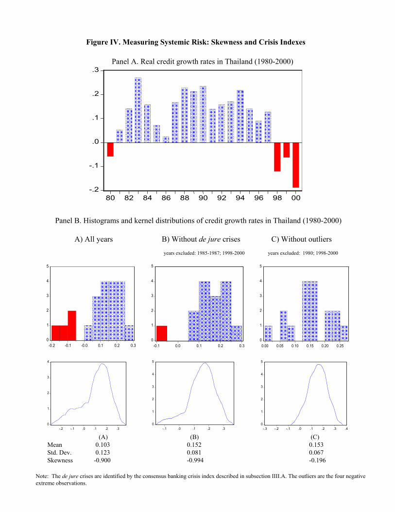
Panel A. Real credit growth rates in Thailand (1980-2000)
80 82 84 86 88 90 92 94 96 98 00-.2
-.1
.0
.1
.2
.3
Panel B. Histograms and kernel distributions of credit growth rates in Thailand (1980-2000)
A) All years B) Without de jure crises C) Without outliers
years excluded: 1985-1987; 1998-2000 years excluded: 1980; 1998-2000
0
1
2
3
4
5
-0.2 -0.1 -0.0 0.1 0.2 0.3
0
1
2
3
4
5
0.00 0.05 0.10 0.15 0.20 0.25
0 1 2 3 4 5
-0.1 0.0 0.1 0.2 0.3
0
1
2
3
4
-.2 -.1 .0 .1 .2 .30
1
2
3
4
5
-.1 .0 .1 .2 .3
0
1
2
3
4
5
-.3 -.2 -.1 .0 .1 .2 .3 .4
(A) (B) (C)Mean 0.103 0.152 0.153Std. Dev. 0.123 0.081 0.067Skewness -0.900 -0.994 -0.196
Figure IV. Measuring Systemic Risk: Skewness and Crisis Indexes
Note: The de jure crises are identified by the consensus banking crisis index described in subsection IIII.A. The outliers are the four negative extreme observations.