Systematic investigations of calcium phosphates produced ...
201
Systematic investigations of calcium phosphates produced by wet chemistry method and supercritical processing techniques by Midhat Nabil Ahmad Salimi A thesis submitted to the School of Chemical Engineering of the University of Birmingham for the degree of Doctor of Philosophy Chemical Engineering University of Birmingham Edgbaston, Birmingham B15 2TT, UK
Transcript of Systematic investigations of calcium phosphates produced ...

Systematic investigations of calcium
phosphates produced by wet chemistry
method and supercritical processing
techniques
by Midhat Nabil Ahmad Salimi
A thesis submitted to the School of Chemical Engineering of the
University of Birmingham
for the degree of
Doctor of Philosophy
Chemical Engineering
University of Birmingham
Edgbaston, Birmingham
B15 2TT, UK

University of Birmingham Research Archive
e-theses repository This unpublished thesis/dissertation is copyright of the author and/or third parties. The intellectual property rights of the author or third parties in respect of this work are as defined by The Copyright Designs and Patents Act 1988 or as modified by any successor legislation. Any use made of information contained in this thesis/dissertation must be in accordance with that legislation and must be properly acknowledged. Further distribution or reproduction in any format is prohibited without the permission of the copyright holder.

Abstract
Calcium phosphate (CaP) based material, especially hydroxyapatite (HAp) nanoparticles
have a wide range of applications in a number of fields, such as drug delivery, gene therapy,
bone cements, dental applications, chromatography and waste water remediation. Depending
on the application, there is often a need for the nanoparticles to be in a particular size range.
One of the potential applications of HAp is for drug delivery; as a transfection vector in
specific. The main aim of this study was to evaluate the potential of various produced CaP
nanoparticles for this matter. The HAp and CaP nanoparticles in this study were
systematically investigated and produced by several methods, firstly by the wet chemistry
method of sol-gel, where the process conditions of varying its stirring rates and temperatures
were taken into consideration; secondly by the supercritical fluid techniques of Gas Anti-
Solvent (GAS) and Solution Enhanced Dispersion of Supercritical Fluids (SEDS), where the
process conditions of varying the processing temperature, pressure and supply of antisolvent
flowrate were investigated. Lastly, several phases of CaPs were produced by a systematic
investigation of CaP precipitation processes (via direct precipitation method and SEDS
processing technique) by varying the Ca/P ratios. The processing conditions such as the
stirring rate, temperature, pressure and antisolvent flowrate played a significant role on the
nanoparticle size and morphology. The produced HAp and CaP nanoparticles were then
complexed with plasmid DNA (pDNA) to evaluate the pDNA binding efficiencies and thus
their potential as a transfection vector in NIH/3T3 fibroblastic and MC3T3 osteoblastic cell
lines via in-vitro transfection study. It had been shown that the particle size played a
significant role on the pDNA binding efficiencies and also on the green fluorescence protein
(GFP) expression in the transfection results obtained.
i

Acknowledgments
This thesis would not have been possible unless with the superior encouragement, guidance
and support from my wonderful supervisors, Dr. Gary A. Leeke, Dr. Liam M. Grover and Dr.
Rachel H. Bridson, from the initial to the final level enabled me to develop an understanding
of the subject.
I would like to thank to the academic staff in the School of Chemical Engineering, including
Dr. Ping Ding, Dr. Shangfeng Du and Dr. James Bowen. I would also like to thank Dr.
Adrian Wright who is in the School of Chemistry for the usage of the XRD facility. I would
like to express my gratitude to all technicians and staff who have helped with a number of
aspects of my PhD in Biochemical Engineering, School of Chemistry and Centre for
Microscopy. Especially, thank to Dr. Jennifer Paxton, Mrs. Elaine Mitchell and Mrs. Theresa
Morris.
Most importantly, I would like to thank my parents, Dato’ Haji Ahmad Salimi Ismail and
Datin Badriyah Md. Tamin who are always near to my heart and for their continuing
emotional support and encouragement.
Lastly, I offer my regards and blessings to all of those who supported me in any respect
during the completion of the project, especially to Norsyafina Roslan, who had been through
thick and thin of this wonderful journey.
Thank you.
Midhat Nabil Ahmad Salimi ii

Table of contents
Chapter 1 Introduction ..............................................................................................................1
1.1 The production of calcium phosphate for biomedical usage …………………....……...…1
1.2 Objectives of the Present Work ……………………………...……………………………2
Chapter 2 Literature Survey ......................................................................................................3
2.1 Types of calcium phosphates ..............................................................................................3
2.1.1 Calcium phosphates ..............................................................................................4
2.1.2 Monocalcium phosphate (monohydrate and anhydrous) .....................................9
2.1.3 Dicalcium phosphate (dehydrate – brushite and anhydrate – monetite) ..……..10
2.1.4 Octacalcium phosphate ………………………………………………………...11
2.1.5 Tricalcium phosphates and whitlockite ………………………………………..12
2.1.6 Hydroxyapatite ………………………………………………………………...13
2.1.7 Tetracalcium phosphate (Hilgenstockite) ……………………………………...17
2.2 Particle formation ………………………………………………………………………..19
2.2.1 The effect of temperature on particle size ……………………………………..24
2.2.2 The effect of stirring rate on the particle size ………………………………….24
2.3 Supercritical fluid processing ……………………………………………………………25
2.3.1 Definition of a supercritical fluid ……………………………………………...26
2.3.2 Particle production techniques using supercritical carbon dioxide (scCO2) …..30
2.3.2.1 Particles prepared by RESS and PGSS ……………………………………...31
2.3.2.1.1 RESS (Rapid Expansion of a Supercritical Solution) ……………..31
2.3.2.1.2 PGSS (Particles from Gas – Saturated Solution) ………………….33
iii

2.3.2.2 Particles prepared by antisolvent techniques, GAS, SAS and SEDS ………..35
2.3.2.2.1 GAS (Gas Anti-Solvent) …………………………………………..35
2.3.2.2.2 SAS (Supercritical Anti-Solvent) ………………………………….37
2.3.2.2.3 SEDS (Solution Enhanced Dispersion of Supercritical Fluids) …...40
2.4 Layout of this Thesis ……………………………………...……………………………..44
2.5 References ……………………………………………………………………………….45
Chapter 3 Hydroxyapatite (HAp) prepared by Sol-gel method ..............................................52
3.1 Introduction .......................................................................................................................52
3.2 Experimental ……………………………………………………………………….……53
3.2.1 Materials and methods ………………………………………………………...53
3.2.1.1 Preparation of Hydroxyapatite particles ….……………..….………..54
3.2.1.2 Preparation of Hydroxyapatite particles with Mg2+
(HAp – Mg) …...55
3.3 Particle characterisation techniques ……………………………………………………..56
3.3.1 Fourier Transform Infrared Spectroscopy (FTIR) ……………………………..56
3.3.2 X-ray Diffraction (XRD) ………………………………………………………56
3.3.3 Scanning Electron Microscopy (SEM) ………………………………………...57
3.3.4 Transmission Electron Microscope (TEM) ……………………………………57
3.3.5 Dynamic Light Scattering (DLS) ……………………………………………...58
3.4 Results and discussion …………………………………………………………………...59
3.4.1 Fourier Transform Infrared Spectroscopy (FTIR) ……………………………..59
3.4.2 X-ray Diffraction (XRD) ………………………………………………………63
3.4.2.1 Hydroxyapatite – sintered …………………………………………...63
3.4.2.2 Mg intercalated calcium phosphate – sintered ………………………64
iv

3.4.2.3 Hydroxyapatite – pre-sintered ………………………………...……..65
3.4.3 Scanning Electron Microscopy (SEM) ………………………………………...66
3.4.4 Transmission Electron Microscope (TEM) ……………………………………69
3.4.5 Dynamic Light Scattering (DLS) ……………………………………………...73
3.4.6 Effect of agitation rate on particle size ………………………………………...76
3.4.7 Effect of temperature …………………………………………………………..79
3.5 Conclusions ……………………..……………………………………………………….82
3.6 References ……………………………………………………………………………….83
Chapter 4 Hydroxyapatite (HAp) prepared by Anti-solvent processing .................................86
4.1 Introduction ……………………………………………………………………………...86
4.1.1 SCF methods selection ....……………………………………………………...87
4.1.1.1 Gas Anti-Solvent (GAS) method ……………………………………87
4.1.1.2 Solution Enhanced Dispersion by Supercritical fluids (SEDS) ……..89
4.1.2 Solvent selection ………………………………………………………………91
4.1.2.1 Classes of solvents …………………………………………………..91
4.1.2.2 Solvent screening ……………………………………………………91
4.1.2.3 Dimethyl sulfoxide (DMSO) ………………………………………..93
4.2 Experimental ………………………………………………………………………….....95
4.2.1 Materials and methods ………………………………………………………...95
4.2.1.1 Preparation of HAp particles by GAS method ………………………95
4.2.1.2 Preparation of HAp particles by SEDS method ……………………..96
v

4.3 Particle characterisation techniques ……………………………………………………..98
4.4 Results and discussion ……………………………………………………………….......99
4.5 Conclusions …………..…………………………………………………………...……107
4.6 References ………………………………………………………………………...……108
Chapter 5 A systematic investigation of Calcium Phosphates (CaP) precipitation
processes ………………………………………………………………………....................110
5.1 Introduction …..…………………………………………………………………...……110
5.2 Materials and methods ……………………………………………………………...….110
5.2.1 Materials …………………………………………………………….………..110
5.2.2 Direct precipitation method ……………………………………..……………111
5.2.3 SEDS method ………………………………………………………….…..…112
5.2.4 Particle characterisation techniques ……………………………………….…113
5.3 Results and discussion ………………………………………………………………....113
5.3.1 Effect of molar ratios on the precipitates collected …………………………..113
5.3.1.1 Direct precipitation method ……………………………………..….113
5.3.1.2 SEDS method …………………………………………………..…..117
5.3.1.3 Ca/P phase formation …………………………………………..…..119
5.3.2 Effect of molar ratios on particle size and morphology …………..……….…123
5.3.2.1 Direct precipitation method ………………………………………...123
5.3.2.2 SEDS method ………………………………………………………125
5.4 Conclusions ………………………………………………………………………...…..126
5.5 References ……………...………………………………………………………………127
vi

Chapter 6 Attachment of calcium phosphate particles prepared by sol-gel, supercritical anti-
solvent and new calcium phosphate route with plasmid DNA (pDNA) and in-vitro
transfection studies of CaP-pDNA post co-precipitation complexes …………………...….129
6.1 Introduction ……………………………………………………………………….……129
6.2 Experimental methods ………………………………………………………………….130
6.2.1 pDNA attachment ……………………………………………………...……..130
6.2.1.1 In-situ co-precipitation attachment by GAS Anti-Solvent (GAS) and
Solution Enhanced Dispersion by Supercritical fluids (SEDS) techniques ..130
6.2.1.2 Post co-precipitation attachment of pDNA on calcium phosphates (CaP)
particles produced by other processing techniques ...…………………….....132
6.2.2 Gel electrophoresis ………………………………………………………...…132
6.2.3 Binding efficiency analysis (pDNA mass balance) …………………..………134
6.2.4 In –vitro transfection studies ...…………………………………………...…..135
6.2.4.1 Materials ...…………………………………………….....................135
6.2.4.2 Cell culture preparation ...……………………………………......... 135
6.2.4.3 CaP-pDNA complexes preparation and in-vitro transfection
procedure…………………………………………………………. 136
6.3 Results and discussion ………………………………………………………………….137
6.3.1 pDNA attachment in-situ onto particles using the GAS and SEDS
techniques …..………………………………………………………………...137
6.3.2 pDNA post co-precipitation attachment …………………………………...…139
6.3.3 Binding efficiencies …………………………………………………………..141
6.3.4 Comparison of analytical data from the post co-precipitation attachment of sol-
gel, anti-solvent methods (GAS & SEDS) and new CaP route with pDNA ……….144
vii

6.3.5 GFP expression ……………………………………………………...……….146
6.3.6 Fluoresence quantification ……………...……………………………………151
6.4 Conclusions …………………………………………………………………………….154
6.5 References ……………………………………………………………………….……..156
Chapter 7 Overall conclusions ..............................................................................................158
Chapter 8 Future work ...........................................................................................................162
8.1 More characterisation of the produced HAp and CaP nanoparticles ..............................162
8.2 HAp produced by other supercritical processing techniques ..........................................162
8.3 In-vivo study of the CaP-pDNA complex ……………………………………………...163
Chapter 9 Appendix ..............................................................................................................164
viii

List of Figures
Figure 2.1 Solubility isotherm of calcium phosphate phases in the ternary system Ca(OH)2-
H3PO4-H2O at 37 oC; log [Ca] versus pH [reproduced from Hoffmann
(2003)] ...........................................................................................................................7
Figure 2.2 pH variation of ionic concentration for phosphoric acids solutions [Lynn &
Bonfield (2003)] ............................................................................................................8
Figure 2.3 Incorporation of crystal forming elements on the surface of a growing crystal
[Sangwal (1998)] .........................................................................................................21
Figure 2.4 a – c Two dimensional growth [Mullin (1961)] ...................................................22
Figure 2.5 Spiral growth from a screw [Burton et al. (1951)] ................................................23
Figure 2.6 Generic phase diagram illustrating critical point and supercritical phase region
[York (1999)] ........................................................................................................27
Figure 2.7 Illustration of reduced complexity of supercritical fluid processing for
nano and microparticle formation [York (1999)] ..................................................29
Figure 2.8 Schematic diagram of RESS equipment ...............................................................32
Figure 2.9 Schematic diagram of PGSS equipment ...............................................................33
Figure 2.10 Schematic diagram of GAS equipment ...............................................................36
Figure 2.11 Schematic diagram of SAS equipment ...............................................................38
Figure 2.12 A typical SEDS coaxial nozzle diagram .............................................................40
Figure 2.13 Schematic diagram of SEDS equipment .............................................................41
Figure 3.1 FTIR spectra for some of HAp samples produced at 20 oC ..................................59
Figure 3.2 FTIR spectra for some of HAp samples produced at 40 oC ..................................60
Figure 3.3 FTIR spectra for 60 mM MgCl2 at 200, 2200 and 7000 rpm ................................62
Figure 3.4 FTIR spectra for 140 mM MgCl2 at 200, 2200 and 7000 rpm ..............................62
Figure 3.5 XRD patterns for some of HAp samples produced at 20 oC .................................63
Figure 3.6 XRD patterns for some of HAp samples produced at 40 oC .................................64
Figure 3.7 XRD patterns of hydroxyapatite samples prepared with 0 mM, 20 mM, 80 mM
and 140 mM MgCl2 at 2200 rpm and 20 oC .........................................................65
Figure 3.8 XRD spectra of a pre-sintered HAp sample produced at 1200 rpm and 20 oC .....66
Figure 3.9 SEM of pre-sintered HAp particles produced at 2200 rpm and 20 oC ..................67
ix

Figure 3.10 SEM of pre-sintered intercalated HAp-Mg particles produced using 140 mM
MgCl2. The crystallinity decreased slightly from 63% without MgCl2 to 58%
(as calculated from Equation 3.2) when 140 mM was added .............................67
Figure 3.11 SEM images of HAp after processing at different agitation rates and
temperatures .......................................................................................................69
Figure 3.12 Effect of Power on Particle size (nm) at 20 oC and 40
oC ..................................77
Figure 3.13 Influence of Re Numbers on Particle size (nm) at 20 oC and 40
oC ...................77
Figure 3.14 Effect of Mg2+
intercalation on HAp particle size for different MgCl2
concentrations and agitation rates at 20 oC .........................................................81
Figure 4.1 Schematic diagram of the GAS rig .......................................................................88
Figure 4.2 Schematic diagram of the SEDS rig .....................................................................90
Figure 4.3 The SEDS coaxial nozzle diagram used in this work ...…………………………90
Figure 4.4 Data of CO2 interaction with DMSO [Lucien et al. (2004)] .................................94
Figure 4.5 FTIR spectra of some GAS & SEDS processed HAp samples ...........................100
Figure 4.6 XRD patterns of some GAS & SEDS HAp samples ..........................................101
Figure 4.7 SEM images of some of the GAS and SEDS samples ........................................104
Figure 4.8 TEM images of some of the GAS and SEDS samples .......................................106
Figure 5.1 XRD patterns of the precipitates for the Ca/P ratios of 2.50, 1.67 and 1.33 .......114
Figure 5.2 XRD patterns of the precipitates for the Ca/P ratios of 1.00, 0.75 and 0.40 .......115
Figure 5.3 FTIR spectra for the precipitates from the direct precipitation method for Ca/P
ratios of 2.50, 1.67, 1.33, 1.00, 0.75 and 0.40 .....................................................116
Figure 5.4 XRD patterns of the precipitates from the SEDS method for Ca/P ratios of 3.00,
1.00 and 0.33 .......................................................................................................118
Figure 5.5 FTIR spectra for the precipitates produced by the SEDS method for Ca/P ratios of
3.00, 1.00 and 0.33 ..............................................................................................119
Figure 6.1 Gel electrophoresis of in-situ co-precipitation of GAS technique particles with
pDNA. Lane 1: M.W. marker, Lane 2 - 4: GAS at 40 oC, 50
oC and 60
oC in-situ
(i.e under pressure) co-precipitation. All GAS samples were carried out at a
pressure of 150 bar ..............................................................................................138
x

Figure 6.2 Gel electrophoresis of HAp post co-precipitation with pDNA for sol-gel and GAS
particle processing methods. Lane 1: M.W. marker, Lane 2: HAp prepared by sol-
gel at 200 rpm, Lane 3: HAp prepared by sol-gel at 2200 rpm, Lane 4: HAp
prepared by sol-gel at 7000 rpm, Lane 5: HAp prepared by GAS at 40 oC, Lane 6:
HAp prepared by GAS at 50 oC and Lane 7: HAp prepared by GAS at 60
oC. All
GAS samples were carried out at a pressure of 150 bar ......................................140
Figure 6.3 Gel electrophoresis of new CaP route post co-precipitation with pDNA. Lane 1:
M.W. marker, Lane 2: CaP prepared by direct precipitation with Ca/P ratio of
0.40, Lane 3: CaP prepared by direct precipitation with Ca/P ratio of 1.00, Lane 4:
CaP prepared by direct precipitation with Ca/P ratio of 2.50, Lane 5: CaP
prepared by SEDS method with Ca/P ratio of 0.33, Lane 6: CaP prepared by
SEDS method with Ca/P ratio of 1.00 and Lane 7: CaP prepared by SEDS method
with Ca/P ratio of 3.00 ........................................................................................140
Figure 6.4 Transfection efficiencies of the CaP-pDNA complexes which were compared to
PolyFect in NIH/3T3 fibroblast cells. ...............................................................151
Figure 6.5 Transfection efficiencies of the CaP-pDNA complexes which were compared to
PolyFect in MC3T3 osteoblast cells. .................................................................152
xi

List of Tables
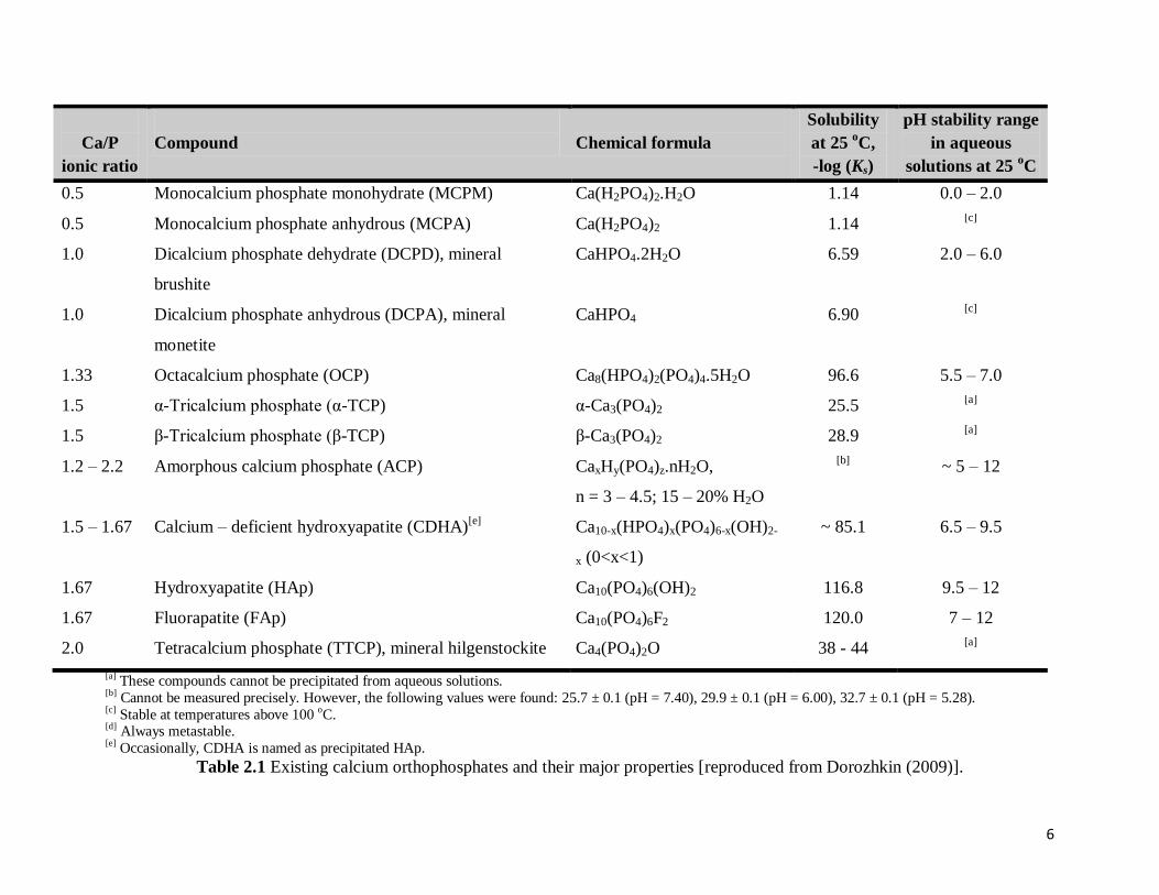
Table 2.1 Existing calcium orthophosphates and their major properties [reproduced from
Dorozhkin (2009)] ....................................................................................................6
Table 2.2 Chemical composition of human bone and HAp [reproduced from Dorozhkin et al.
(2007)] .....................................................................................................................14
Table 2.3 Positions of different vibrations of hydroxyl, phosphate, and carbonate in FTIR
analysis of HAp and carbonated substituted apatite (CHAp) .................................17
Table 2.4 Critical values of some common substances [Reid et al. (1987)] ..........................26
Table 2.5 Typical selected properties for materials in gas, liquid and supercritical phases
[reproduced from Raynie (1997)] ...........................................................................28
Table 2.6 Comparison of various SCF particle processes [Knez (2000)] ..............................42
Table 3.1 TEM images and particle size estimations based upon the images and Scherrer’s
formula (Eqn. 1) for HAp samples produced with the overhead stirrer .................71
Table 3.2 TEM images and particle size estimations based upon the images and Scherrer’s
formula (Eqn. 1) for HAp samples produced with the homogeniser .....................72
Table 3.3 Particle size measurement by DLS (unfiltered) ......................................................74
Table 3.4 Particle size measurement by DLS (filtered) ..........................................................75
Table 4.1 Solubility (x1) of CO2 (1) in DMSO (2) at various temperatures ...........................94
Table 4.2 GAS experimental conditions ……………………………………………………95
Table 4.3 SEDS experimental conditions ...............................................................................97
Table 4.4 Particle sizing for HAp produced by GAS technique ...........................................102
Table 4.5 Particle sizing for HAp produced by SEDS technique .........................................103
Table 5.1 Ca/P molar ratio studied for the direct precipitation method ...............................113
Table 5.2 Ca/P molar ratios studied for the SEDS method ..................................................117
Table 5.3 SEM, TEM & DLS particle size data obtained from the direct precipitation
method ..................................................................................................................124
Table 5.4 SEM, TEM and DLS particle size data obtained from the SEDS method ...........125
Table 6.1 Binding efficiency data of various CaP-pDNA complex .....................................143
Table 6.2 Fluorescence light micrographs of NIH/3T3 fibroblast and MC3T3 osteoblast cell
lines transfected with some of the CaP-pDNA complexes ………......................147
xii


1
1.0 Introduction
Specific characteristics of particles (size, shape, surface, crystal structure and morphology) are
among the important factors needed to control technological and biopharmaceutical properties of
drug products. In general, morphology (crystal habit) can influence the physical and chemistry
stability of solid dosage forms, a narrow size distribution is important to obtain content
uniformity, while spherical particles allow good flowability and tablettability. Furthermore,
micronisation increases the surface area with a consequent increase of dissolution rate and
bioavalability of the drug, thus promoting the formulation of active principle ingredients which
may be insoluble or slightly soluble in aqueous media.
1.1 The production of calcium phosphate for biomedical usage
Calcium phosphate nanoparticles have a range of applications in a number of fields, such as drug
delivery, gene therapy, bone cements, dental applications, chromatography and waste water
remediation. Each application has a need for the nanoparticles to be of a particular size range.
There are various techniques reported in the literature for the production of nanosized calcium
phosphate particles. These include mechano-chemical synthesis [Kano et al. (2006)], combustion
preparation [Tas (2000)], and various wet chemistry techniques, such as direct precipitation from
aqueous solutions [Rodriquez-Clemente et al. (2000)], sol-gel procedures [Weng & Baptista
(1997)], hydrothermal preparation [Yoshmura et al. (1994)] and emulsion synthesis routes [Lim
et al. (1999)]. The production of this material by supercritical fluid processing has never been
reported. It is anticipated that by this method, particles can be produced with higher purity,
different morphology, narrow size distribution and fewer processing steps.

2
1.2 Objectives of the Present Work
The objectives of this work were firstly to examine the literature and summarise the background
to supercritical fluid technology and the work carried out to date in the area of particle formation.
Secondly, to construct a suitable apparatus to study the production of calcium phosphate based
biomaterial powders using supercritical carbon dioxide as an anti-solvent under various
conditions. These powders were to be characterised using a variety of analytical techniques to
obtain information on their physical properties such as its chemical phase, functional groups,
particle size and morphology. Objectives also cover the investigations of process parameters of
wet chemistry precipitation, the comparison of particles produced by wet chemistry precipitation
to supercritical fluid (SCF) processing and loading of calcium phosphate (CaP) particles with
plasmid DNA (pDNA) to test efficacy as potential gene vector in in vitro transfection studies.

3
2.0 Literature Survey
2.1 Types of calcium phosphates
Calcium phosphates are of interest for many biomedical applications owing to their good
biocompatibility and bioactivity. Hydroxyapatite (HAp) has been used in implant coatings [Sun
et al. (2001)] and bone substitutes [LeGeros (1991)]. Amorphous calcium phosphate (ACP) are
used as remineralisation agents both in-situ [Tung et al. (1997)] and in tooth restorative materials
[Skrtic et al. (2004)]. Dicalcium phosphate anhydrous (DCPA) and dicalcium phosphate
dehydrate (DCPD) [Brown & Chow (1986)], octacalcium phosphate (OCP) [Bermudez et al.
(1994)] and other calcium phosphate compounds [Mejdoubi et al. (1994), Ginebra et al. (1997),
Lee et al. (1999)] are used either as components or form as products of calcium phosphate bone
cements.
Previous studies on nano-calcium phosphates have focused almost exclusively on nano-HAp,
primarily because it is considered as a prototype of bioapatites, which are in nano-crystalline
forms [LeGeros (1991)]. Most of these preparations were done in a solution environment, such
as chemical precipitation [Tas (2000) & Bertoni et al. (1998)], sol-gel [Chai & Ben-Nissan
(1994) & Layrolle et al (1998)], microemulsion [Bose & Saha (2003) & Lim et al. (1999)],
electro-deposition [Shirkhanzadeh (1998)], and mechanochemical preparation followed by
hydrothermal treatment [Suchanek et al. (2004)]. These methods generally can be used for
preparing nano-HAp only because HAp is the least soluble calcium phosphate under most
solution conditions; hence it is the phase that would form exclusively [Dorozhkin (2007 &

4
2009)]. Nanoparticles of the more soluble calcium phosphate phases, such as monocalcium
phosphate monohydrate (MCPM), dicalcium phosphate monohydrate (DCPA), dicalcium
phosphate dehydrate (DCPD), octacalcium phosphate (OCP), and amorphous calcium phosphate
(ACP) have not been prepared by these methods. Their preparations are discuss in respective
calcium phosphate phase later in this chapter.
In this section, the details of the existing calcium phosphates are briefly explained, with respect
to their properties and synthesis process methods. Some particle characterisation techniques are
also explained.
2.1.1 Calcium phosphates
By definition, all calcium orthophosphates consist of three major chemical elements; calcium
(oxidation state +2), phosphorus (oxidation state +5) and oxygen (reduction state -2), as part of
orthophosphate anions. There are a large variety of calcium phosphates in existence, which are
distinguished by the type of the phosphate anion: ortho- (PO43-
), meta- (PO3-) or pyro- (P2O7
4-)
and poly- ((PO3)nn-
). Several phases of crystallised calcium phosphates can be formed which
depend on temperature, partial pressure of water and impurities [Dorozhkin (2009)]. The
different phases of calcium phosphate are summarised in Table 2.1. It is interesting to note that,
the lower the Ca/P molar ratio, the more acidic and water soluble the calcium phosphate is, due
to the solubility criteria and the kinetics of precipitate formation and transformation [Elliott
(1994)]. The solubility isotherm profile shown in Figure 2.1 indicates the likely conditions
required for synthesis of a variety of calcium phosphates. The saturation boundary is represented

5
by the curve of each phosphate composition. The calcium phosphate compositions below the
curve are supersaturated, whereas those above are under-saturated. From the figure, it can be
seen that hydroxyapatite (HAp) is the least soluble calcium phosphates at a pH value of > 4.2
(the most stable calcium phosphate phase). Therefore, above this pH all calcium phosphates are
likely to hydrolyse to HAp.
6
Ca/P
ionic ratio
Compound
Chemical formula
Solubility
at 25 oC,
-log (Ks)
pH stability range
in aqueous
solutions at 25 oC
0.5 Monocalcium phosphate monohydrate (MCPM) Ca(H2PO4)2.H2O 1.14 0.0 – 2.0
0.5 Monocalcium phosphate anhydrous (MCPA) Ca(H2PO4)2 1.14 [c]
1.0 Dicalcium phosphate dehydrate (DCPD), mineral
brushite
CaHPO4.2H2O 6.59 2.0 – 6.0
1.0 Dicalcium phosphate anhydrous (DCPA), mineral
monetite
CaHPO4 6.90 [c]
1.33 Octacalcium phosphate (OCP) Ca8(HPO4)2(PO4)4.5H2O 96.6 5.5 – 7.0
1.5 α-Tricalcium phosphate (α-TCP) α-Ca3(PO4)2 25.5 [a]
1.5 β-Tricalcium phosphate (β-TCP) β-Ca3(PO4)2 28.9 [a]
1.2 – 2.2 Amorphous calcium phosphate (ACP) CaxHy(PO4)z.nH2O,
n = 3 – 4.5; 15 – 20% H2O
[b] ~ 5 – 12
1.5 – 1.67 Calcium – deficient hydroxyapatite (CDHA)[e]
Ca10-x(HPO4)x(PO4)6-x(OH)2-
x (0<x<1)
~ 85.1 6.5 – 9.5
1.67 Hydroxyapatite (HAp) Ca10(PO4)6(OH)2 116.8 9.5 – 12
1.67 Fluorapatite (FAp) Ca10(PO4)6F2 120.0 7 – 12
2.0 Tetracalcium phosphate (TTCP), mineral hilgenstockite Ca4(PO4)2O 38 - 44 [a]
[a] These compounds cannot be precipitated from aqueous solutions. [b] Cannot be measured precisely. However, the following values were found: 25.7 ± 0.1 (pH = 7.40), 29.9 ± 0.1 (pH = 6.00), 32.7 ± 0.1 (pH = 5.28). [c] Stable at temperatures above 100 oC. [d] Always metastable. [e] Occasionally, CDHA is named as precipitated HAp.
Table 2.1 Existing calcium orthophosphates and their major properties [reproduced from Dorozhkin (2009)].

7
Figure 2.1 Solubility isotherm of calcium phosphate phases in the ternary system Ca(OH)2-
H3PO4-H2O at 37 oC; log [Ca] versus pH [reproduced from Hoffmann (2003)].
Variations in pH alter the relative concentrations of the four polymorphs of orthophosphoric acid
(Figure 2.2) and thus both the chemical composition and the amount of calcium orthophosphates
that forms by direct precipitation [Lynn & Bonfield (2003)].

8
Figure 2.2 pH variation of ionic concentration for phosphoric acids solutions [Lynn & Bonfield
(2003)].

9
2.1.2 Monocalcium phosphate (monohydrate and anhydrous)
Monocalcium phosphate can either form the monohydrate (MCPM) or anhydrous salt
(MCPA). MCPM has a chemical formula of Ca(H2PO4)2.H2O and its chemically correct
name is calcium dihydrogen phosphate monohydrate. Meanwhile, MCPA has a chemical
formula of Ca(H2PO4)2 and its chemically correct name is calcium dihydrogen phosphate
anhydrous. With a Ca/P ratio of 0.5, MCPM and MCPA are the most acidic and water soluble
calcium phosphates as shown on Table 2.1 [Dorozhkin (2009)].
MCPM can be produced by the ‘triple superphosphate’ reaction for phosphorus-containing
fertilizer production [Becker (1989)]. In this process, MCPM is produced by the reaction of
concentrated phosphoric acid with powdered phosphate rock. At temperatures above 100 oC,
it releases a molecule of water and transforms into MCPA.
The presence of MCPM and MCPA can be distinguished from the peaks of an XRD pattern
at 7o, 23 - 24
o, and 24 - 26
o 2θ. In addition, the HPO4
2- group is present at 870 cm
-1 in the
FTIR spectrum. Both have the crystallographic structure of triclinic space group.
Although MCPM is not biocompatible (due to being the most acidic calcium phosphate
compound), in medicine, it is used as a component of several self-hardening calcium
orthophosphate cements [Bermudez et al. (1994)]. There is no current application of MCPA
in medicine.

10
2.1.3 Dicalcium phosphate (dehydrate - brushite and anhydrate - monetite)
Dicalcium phosphate dihydrate (DCPD) or better known as the mineral brushite can easily be
crystallised from aqueous solutions at pH <6.5. Briefly, DCPD crystals consist of CaHPO4
chains arranged parallel to each other, while lattice water molecules are interlayed between
them. DCPD can be precipitated by mixing a calcium hydroxide, Ca(OH)2 suspension and an
orthophosphoric acid, H3PO4 solution in equimolar quantities at room temperature [Oliveira
et al. (2007)]. DCPD is also formed by neutralising dilute H3PO4 by the addition of calcium
sucrate (calcium carbonate and sucrose) [St. Pierre (1995)]. It transforms into dicalcium
phosphate anhydrous (DCPA) at temperatures above 80 oC. DCPD has the crystallographic
structure of monoclinic space group. In medicine, DCPD is used in calcium orthophosphate
cements [Bermudez et al. (1994)] and as an intermediate for tooth remineralisation. DCPD is
added to toothpaste both for dental caries protection (it is coupled with F-containing
compounds such as NaF and/or Na2PO3F) and as a gentle polishing agent [Crall & Bjerga
(1987)].
Meanwhile, dicalcium phosphate anhydrous (DCPA) or better known as the mineral monetite
is the anhydrous form of DCPD. It is less soluble than DCPD due to the absence of water
inclusions. Unlike DCPD, DCPA occurs in neither normal nor pathological calcifications.
DCPA has the crystallographic structure of triclinic space group. It is used in calcium
phosphate cements [Takagi et al. (1998)]. Other applications include uses as a polishing
agent, a source of calcium and phosphate in nutritional supplements, a tabletting aid and a
toothpaste component [Budavari et al. (1996)].

11
2.1.4 Octacalcium phosphate
Octacalcium phosphate (OCP) has a chemical formula of Ca8(HPO4)2(PO4)4.5H2O and is
often found as an unstable transient intermediate during the precipitation of the
thermodynamically more stable HAp in aqueous solutions. OCP has a similar structure to
HAp, in which it has apatitic layers separated by hydrated layers [LeGeros (1991) & Elliot
(1994)].
OCP can be synthesised by means of homogeneous crystallisation, where a solution of
calcium nitrate tetrahydrate and disodium hydrogen orthophosphate are held at temperatures
between 45 and 55 oC and a pH between 6.49 and 7.15 for 48 h [Shelton et al. (2006)]. Pure
OCP can be precipitated by the addition of calcium acetate to an equal volume of sodium and
phosphorus at pH 4.5 at 70 oC for 1 h or pH 4 at 80
oC for 1 h [LeGeros (1985)]. OCP
hydrolyses to HAp in water, depending on the availability of calcium ions [Elliot (1994)].
The hydrolysis reaction is represented by the chemical formula:
Ca8H2(PO4)65H2O + 2Ca2+
→ Ca10(PO4)6(OH)2 + 3H2O + 4H+
Equation 2.1
OCP has the crystallographic structure of triclinic space group. Intense peaks for OCP on the
XRD patterns are at 26o and 32
o 2θ. It exhibits HPO4
2- bands at 865 and 910 cm
-1 on FTIR
spectra.

12
2.1.5 Tricalcium phosphates and whitlockite
Tricalcium phosphates (TCPs) can exist in either α-TCP or β-TCP crystal form. β-TCP
cannot be precipitated from aqueous solutions. β-TCP can be prepared by addition of Na3PO4
solution to a CaCl2 solution at a Ca/P molar ratio of 1.5. The reaction conditions are at pH
value of 9 and temperature of 5 oC. As it is a high temperature phase, β-TCP can also be
prepared by thermal decomposition (> 800 oC) of calcium defficient HAp (CDHAp) or by
solid-state interaction of acidic calcium orthophosphates, e.g., DCPA with a base, e.g., CaO.
Apart from the chemical preparation route, ion-substituted β-TCP can be prepared by
calcining bones: such types of β-TCP are occasionally called “bone ash” [Dorozhkin (2009)].
α-TCP is stable at temperatures between 1180 – 1400 oC and is formed by the phase
transformation of β-TCP. At temperatures above ~ 1125 oC, β-TCP transforms into the high-
temperature phase, α-TCP. Whitlockite is the Mg-substituted form of β-TCP.
Although α-TCP and β-TCP have exactly the same chemical composition, they differ in term
of their solubility, where β-TCP is found to be more stable than the α-phase [Yin et al.
(2003)]. Hence, α-TCP is more reactive in aqueous systems, has higher specific energy and
can be hydrolysed to a mixture of other calcium phosphates. α-TCP has the crystallographic
structure of monoclinic space group, meanwhile, β-TCP has the crystallographic structure of
rhombohedral space group.
β-TCP is widely used as calcium orthophosphate bone cements [Mirtchi et al. (1990)], gentle
polishing agent in toothpaste and complexes in multivitamin. Meanwhile, α-TCP is used
mainly as calcium orthophosphate cements [Bermudez et. al. (1994)]. In terms of FTIR

13
analysis, the phosphorus absorption (P-O) is present at 600 cm-1
as a single band for α-TCP,
but at 550 and 616 cm-1
as split bands for β-TCP. For whitlockite, there is a P-OH stretching
band at 850 cm-1
[Elliott (1994)]. In terms of XRD, it is denoted by the peak occurring at 22o
and the overlapping of peaks at 2θ range of 31.7 – 33o.
2.1.6 Hydroxyapatite
Hydroxyapatite (HAp) has the chemical formula of Ca5(PO4)3(OH), but is usually written as
Ca10(PO4)6(OH)2 as to denote that the crystal unit cell comprises of two molecules. HAp is
the second most stable and least soluble calcium orthophosphate in water with a Ks of –log
116.8 after fluoroapatite, FAp; Ks of –log 120.0 (refer to Table 2.1). Pure HAp has a
stoichiometric Ca/P ratio of 1.67, above this, it indicates the presence of calcium rich HAp or
carbonated HAp, whereas, a Ca/P ratio below 1.67 indicates the apatite is calcium deficient
or contains other impurity phases [Hench and Wildson (1993)]. HAp has attracted significant
interest as a biomaterial because of its similarity in composition to the mineral component of
bone [Shi (2004)]. A table comparing both compositions is shown on the next page (Table
2.2):

14
Composition Bone (wt%) HAp (wt%)
Calcium as C 34.80 39.60
Phosphorus as P 15.20 18.50
Ca/P (molar ratio) 1.71 1.67
Sodium 0.90 -
Magnesium 0.72 -
Potassium 0.03 -
Carbonate as CO32- 7.4 -
Fluoride 0.03 -
Chloride 0.13 -
Pyrophosphate as P2O74- 0.07 -
Total inorganic components 65 100
Total organic components 25 -
H2O 10 -
Table 2.2 Chemical composition of human bone and HAp
[reproduced from Dorozhkin et al. (2007)].
Several techniques can be used for HAp preparation, in general, they can be divided into
solid-state reactions (materials chemistry) and wet methods [Briak-Ben et al. (2008)], which
include precipitation, hydrothermal and hydrolysis of other calcium orthophosphates. One of
the wet methods is by mixing exact stoichiometric quantities of Ca- and PO4- containing
solutions at pH > 9, followed by boiling for several days in CO2-free atmosphere (the ageing
or maturation stage), followed by filtration, drying and, usually sintering at about 1000 oC
[LeGeros (1993)].

15
To obtain stoichiometric HAp (s-HAp) by direct precipitation, the reactants used must be
H3PO4 and Ca(OH)2 or salts of calcium and phosphates with ions such as nitrates or
ammonium, which are unlikely to be incorporated in the apatitic phase. Because of the low
solubility of apatites, if the calcium and phosphate ions have exact molar values in the
reaction medium, s-HAp can be obtained.
In the sol-gel technique, HAp powder is obtained by reacting phosphoric pentoxide (P2O5)
and calcium nitrate tetrahydrate (Ca(NO3)2. 4H2O). In this technique, a sintering step at 600
oC was included as to obtain s-HAp [Feng et al. (2005)]. In hydrothermal precipitation, HAp
whiskers were prepared by a precipitation-hydrolysis method in moderately acid solutions at
a temperature between 85 to 95 oC for 48 to 120 h [Zhang et al. (2003)]. In emulsion
synthesis of HAp, calcium hydroxide, Ca(OH)2 aqueous solution was mixed with potassium
dihydrogenphosphate (KH2PO4) for 24 h under intense agitation at 50 oC and calcined at 650
oC for 1 h [Sonoda et al. (2002)].
Hydroxyapatite can be synthesised through solid-state reaction by using calcium
pyrophosphate (Ca2P2O7) and calcium carbonate (CaCO3). The two powders were mixed in
acetone and water, respectively, and the single phase of hydroxyapatite was observed to
occur during heat treatment at 1100 oC for 1 h [Rhee (2002)].
The deposition of HAp coatings onto prostheses can be accomplished by spontaneously
nucleating and growing HAp using metastable synthetic body fluids composed of an
inorganic salt composition [Ferraz et al. (2004)]. The thickness of HAp coating is usually in

16
the range of 200 to 400 μm. Other techniques of HAp coating include plasma spraying,
sputter coating, laser deposition and sol-gel processing. Plasma spraying uses a stream of gas
such as pure argon or a mixture of argon and other gases to carry HAp powders, which are
then passed through plasma produced using a low voltage, and high current electrical
discharge. Plasma spraying, however has its own problems including: binding between
coatings and the substrates, and the alteration of HAp structure [Yang et al. (2005)]. Like
plasma spraying, sputter coating deposits HAp layers on the substrate, but with low pressure
during sputtering. Laser deposition uses an active medium to produce the optical gain under
proper pumping conditions, and the optical resonator is composed of a pair of mirrors and
reflects to produce optical feedback and amplified beam [Paital et al. (2008)].
The crystallographic structure of HAp could either be monoclinic or hexagonal space group.
The FTIR spectra of HAp has been summarised in Table 1.3 [Elliot (1994)]. HAp has a
characteristic HPO42-
ion adsorption at 870 cm-1
. However, the carbonate ion absorption
appears at 870 cm-1
because of the out-of-plane stretching. Therefore, it will interfere with the
analysis of HAp. In addition to PO43-
bands, the OH- band is expected at 3600 cm
-1.

17
Sample
PO43-
ν1
Stretching
mode
(cm-1
)
PO43-
ν2
Vibration
mode
(cm-1
)
PO43-
ν3
Stretching
mode
(cm-1
)
PO43-
ν4
Bending
mode
(cm-1
)
CO32-
ν2
Vibration
mode
(cm-1
)
CO32-
ν2
Stretching
mode
(cm-1
)
CO32-
ν2
Bending
mode
(cm-1
)
OH-
Rotary
mode
(cm-1
)
HAp 963 470 1029
1092
536
603
876 - - 635
679
CHAp 960 - 1023 561
603
875 1409
1486
- -
Table 2.3 Positions of different vibrations of hydroxyl, phosphate, and carbonate in FTIR
analysis of HAp and carbonated substituted apatite (CHAp).
HAp is widely used as a coating on orthopaedic prostheses, and also with biological
components (e.g. pDNA) for drug delivery due to the similarity to bone and teeth [Dorozhkin
(2007)].
2.1.7 Tetracalcium phosphate (Hilgenstockite)
Tetracalcium phosphate (TTCP or TetCP) has a Ca/P ratio of 2.0 and is the most basic among
all of the existing calcium phosphate orthophosphates. However, its solubility in water is
higher than that of HAp. TTCP can not be synthesised in an aqueous environment (owing to
the oxygen atom in its formula, Ca4(PO4)2O [Jalota et al. (2005)], precipitates formed in basic
aqueous solutions will incorporate hydroxyl ions, and therefore, always consist of carbonate-
and/or hydroxyl ion-containing apatitic phases. Hence, common methods for the synthesis of
TTCP are limited to solid-state reactions at high temperatures [Matsuya et al. (1999)]. These
methods are usually based on mixtures of calcium carbonate (CaCO3) and dicalcium
phosphate anhydrate (CaHPO4), which are then heated to 1400 – 1500 oC for 6 – 12 h. The
reaction is given by the following equation:

18
2CaHPO4 + 2CaCO3 → Ca4(PO4)2O + 2CO2 + H2O Equation 2.2
After heating, the mixture must be rapidly quenched to room temperature in order to avoid
the formation of undesired secondary phases, such as HAp, CaO, CaCO3 and β-TCP. TTCP
has the monoclinic space group.
Miao et al. [Miao et al. (2204)] have reported on the use of TTCP as scaffolds in tissue
engineering.

19
2.2 Particle formation
In a crystallisation process, size and morphology are regarded as important properties of the
crystalline product. One of the main aims of the crystallisation process can be for the
synthesis of single crystals of very small size, if a high specific surface area is the desired
property. Crystallisation process involves complex mechanisms but its theories can be
simplified into 3 major steps which are achievement of supersaturation or supercooling,
nucleation (formation of crystal nuclei) and crystal growth [Mackellar et al. (1994)]. The
achievement of supersaturation can be done by cooling or evaporating a solution or by the
addition of other substance(s), such that a deviation from equilibrium solubility is achieved.
The crystal development is initiated by the collision of molecules of solute that form embryos
[Florence & Attwood (1998)]. When solute molecules aggregate around each other and when
nuclei occur spontaneously, nucleation is termed homogeneous. Embryos can also be formed
by the addition of a seed crystal, a dust particle or by migrated particles from a container’s
wall. This is termed heterogeneous nucleation and occurs when nuclei are induced artificially.
Homogeneous and heterogeneous mechanisms form the primary nucleation [Mullin (2000)].
Surface energy, temperature and supersaturation are the most important variables that affect
nucleation [Myerson & Ginde (1993)]. In heterogeneous nucleation, the consequences of
added solid particles reduce the surface free energy and thus induce nucleation.
Secondary nucleation results from the presence of solute particles in a supersaturated solution
[Boistelle & Astier (1998)]. The solute crystals catalyse the nucleation; hence, nucleation
occurs at relatively low supersaturation. Secondary nucleation has been recognised as being
the major source of nuclei in many industrial crystallisers.

20
The next step of nucleation in a crystallisation process is crystal growth. The crystal growth is
governed by a 4-step process, by which a growth unit passes from the bulk solution to the
crystal lattice. Initially, the growth unit moves from the bulk solution to the crystal surface,
where it adsorbs onto the surface. Then, possible diffusion of the growth units to a more
favourable site may occur. Finally, growth units integrate into the crystal lattice [Zipp &
Rodríguez (1993)]. The rate-limiting steps for crystal growth are generally considered to be
the rate of transport of growth units to the crystal surface (diffusion-controlled) and/or
integration into the crystal lattice [Mackellar et al. (1994)].
Adsorption of the crystal forming elements (depicted as a cube) on the surface structure of a
growing crystal may occur at three possible sites [Sangwal (1998)]:
[1] Ledge sites (incorporation at a flat surface (terrace) having only one site of intermolecular
interaction available),
[2] Step sites (incorporation at a surface having two sites of intermolecular interactions
available), or
[3] Kink sites (three possible sites of intermolecular interactions).

21
Figure 2.3 Incorporation of crystal forming elements on the surface of a growing crystal
[Sangwal (1998)].
Because crystal forming elements with the highest coordination number are bound most
strongly to the surface, incorporation at a kink site will provide a new kink site; the kink site
is thus a ‘repeatable-step’ in the formation of the crystal. For example, HAp
(Ca10(PO4)6(OH)2) has Ca2+
as its central cation, which has a coordination number of 8.
Crystal growth can follow two possible mechanisms, two-dimension nucleation or spiral
growth at screw-dislocations. In two-dimension growth, before growth can occur a
monolayer island nucleus, usually called a ‘two-dimensional nucleus’, must come into
existence on an existing layer (Figure 2.4 a). This island becomes the source of new steps and
kink sites at which additional units can join the surface. Subsequent crystal forming elements
will tend to incorporate at sites where attractive forces are greatest, i.e. they will migrate
towards the energetically favourable kink sites (Figure 2.4 b). The step-growth will advance
until the whole plane is completed (Figure 2.4 c) and a new two-dimensional nucleus has to
be generated before growth can advance [Mullin (1961), Garside & Davey (2000)].

22
Figure 2.4 a – c Two dimensional growth [Mullin (1961)].
At low supersaturation, growth occurs along screw dislocations (Burton-Cabrera-Frank
(BCF) model) [Burton et al. (1951)]. This model (Figure 2.4 a, b and c) is based on a defect
in the structure of the crystal lattice formed by stress inside the crystal lattice, which produces
spiralling mounds. From Figure 2.5, it can be seen that these screw dislocations in the crystal
are a continuous source of new steps and that this screw mechanism provides a way for steps
to grow uninterrupted.

23
Figure 2.5 Spiral growth from a screw [Burton et al. (1951)].
Significant changes in the particle size, shape and purity can be due to minor changes of the
crystallisation conditions, such as supersaturation, cooling rate and impurities. A condition
where supersaturation is very high and fast will dramatically affect the nucleation rate, which
usually leads to a decrease in the mean size of the particles.
Surfactants are commonly used in pharmaceutical suspensions in order to lower the
interfacial tension between the solid and the solvent facilitating wetting of the solid. They can
also be used as colloids to improve the stability of the suspension. Surfactants have been
found to promote, to slow down, or to prevent crystal growth in solutions.

24
2.2.1 The effect of temperature on particle size
Cooling of a solution is one of the most widely used methods for achieving the
supersaturation essential for crystallisation. Cooling temperature is known to influence the
rate of growth and size of crystals through its effect on supersaturation [Jones (1974),
Myerson & Ginde (1993), Mullin (2000), Chernyshev (2009) & Seoudi et al. (2010)]. In
general, the crystal size decreases at higher levels of supersaturation due to increased
nucleation rates. Therefore, a larger number of small crystals can be achieved with low
cooling temperatures. A minor factor influencing the nucleation and crystal growth as the
temperature decreases is the resulting increase in the viscosity of the solution, causing
diminished molecular movement. This, in turn, slows down both nuclei formation and growth
rate on the nuclei formed [Mullin (2000)].
2.2.2 The effect of stirring rate on the particle size
It is known that the stirring rate has a strong influence upon the nucleation rate. While gentle
stirring causes nucleation in solutions that are otherwise stable, strong stirring creates an even
greater tendency to form nuclei [Mullin & Raven (1961)]. The reduced crystal size observed
with increased stirring rates is therefore likely to result from secondary nucleation.
Nucleation has been considered as a 2-step process: first, the diffusional transport step,
followed by integration of molecules into the crystal lattice [Mullin & Raven (1961), Dogua
& Simon (1978)]. Secondary nucleation is critically dependent on stirring rates. It is well
known that as stirring rates increase, so does the secondary nucleation [Mullin (2000)]. It is
also known that the stirring rate has a strong influence upon the nucleation rate of solutions
until a particular stirring rate is reached. After this no increase occurs because solute
diffusion is maximised.

25
2.3 Supercritical fluid processing
Supercritical fluids, the properties of which can be tuned by changing the fluid density
between those of liquid and gases, have been adopted or are being explored as: (a) alternative
solvents for classical separation processes such as crystallisation, adsorption, fractionation,
extraction and chromatography, (b) as reaction media as in polymerisation or
depolymerisation, or (c) simply as a reprocessing fluid as in the production of fibers, particles
or foams. A wide variety of organic and inorganic materials have been processed in the form
of particles, fibers, films and foams, employing supercritical fluids as solvent or antisolvents.
The history of supercritical fluids started when Baron Cagniard de la Tour, a French engineer
and physicist discovered the critical point of a substance in his famous cannon barrel
experiments in 1822 [Berche et al. (2009)]. He observed the critical temperature by listening
to the discontinuities in the sound of a rolling flint ball in sealed cannon filled with fluids at
various temperatures. The densities of the liquid and gas phases become equal above this
temperature and the distinction between them disappears, resulting in a single supercritical
fluid phase. Hanny and Hogarth [Hanny & Hogarth (1879)] are considered as pioneers in
laying the fundamental properties of supercritical fluids, based on their basic concept of
Rapid Expansion of Supercritical Solutions (RESS). They described that when the solid is
precipitated by suddenly reducing the pressure, it is crystalline, and may be brought down as
a ‘snow’ in the gas. This concept was further understood and developed after the pioneering
works of Krukonis [Krukonis (1984)] and especially the Battelle Institute Research team
[Smith et al. (1987)] that described and modelled the flow pattern and nucleation process.
Since the mid 1980s, a lot of work on particle production using supercritical fluids, and
especially supercritical carbon dioxide (scCO2) has been carried out [Jung & Perrut (2001)].

26
Jung and Perrut have described in detail about a number of techniques for the production of
particles using SCFs. These details can be found in section 2.3.2.
2.3.1 Definition of a supercritical fluid
A supercritical fluid (SCF) can be defined as any substance that is above both of its critical
pressure (Pc) and critical temperature (Tc). Some of the common substances and their critical
conditions are shown in Table 2.4.
Name Tc (oC) Pc (bar)
Nitrogen -147.1 33.9
Carbon dioxide 31.0 73.8
Butane 153.0 36.5
Water 374.2 221.9
Table 2.4 Critical values of some common substances [Reid et al. (1987)].

27
Solid Liquid Supercritical fluid
Pressure
Triple point Critical point
Gas
Temperature
Figure 2.6 Generic phase diagram illustrating critical point and supercritical phase
region [York (1999)].
From Figure 2.6, it can be noted that above the critical point condition (denoted by the critical
point), the fluid is no longer in a gas or a liquid phase, but midway between these two phases.
At this condition, it can diffuse into solids like a gas, and dissolve materials like a liquid. This
means that SCFs have higher diffusivities than corresponding liquids and higher densities
than the equivalent gases [Tsutsumi et al. (1995)]. In term of its viscosity, it is lower than that
of the same liquid but more equivalent to that of the gas phase. Close to the critical point,
small changes in pressure or temperature will result in large changes in density, allowing
many properties of a supercritical fluid to be “fine –tuned” [Tsutsumi et al. (1995)]. Table 2.5
shows the density, diffusivity and viscosity for a typical gas, liquid and supercritical phases:

28
Phase Density (kg/m3) Diffusivity (m
2s
-1) Viscosity (Ns m
-2)
Gas 6 -20 (1 – 4) x 10-5
(1 – 3) x 10-5
Liquid 600 - 1600 (2 – 20) x 10-10
(2 – 30) x 10-4
Supercritical 200 - 1000 (2 – 7) x 10-8
(1 – 9) x 10-5
Table 2.5 Typical selected properties for materials in gas, liquid and supercritical
phases [reproduced from Raynie (1997)].
A SCF makes a good solvent due to its density and diffusivity properties (solvating power is
directly linked to density), thus it is the main principle behind the bulk of SCF processing.
Once the system is expanded to atmospheric conditions, the SCF is no longer a solvent thus
causing the solute to disengage. This leaves the solute ‘residue-free’ [Weidner et al. (1994)],
which is of use for industries with high regulatory control, such as the pharmaceutical
industry.
There are many industrial uses for SCFs, such as extraction, chromatography, chemical
reactions, micro and nano particle formation, supercritical water oxidation, supercritical
water power generation, biodiesel production and for storage of carbon capture. An in depth
review on some of these other uses for SCFs can be gained by texts published by McHugh
[McHugh & Krukonis (1994)] and Clifford [Clifford (1999)]. One of the main advantages of
using SCF to produce nano and micro particles is the reduction in the amount of process steps
(mostly being a single step process) as compared to conventional particle production
techniques and the use of milder temperature conditions if the SCF is CO2. Figure 2.7

29
illustrates the comparison between a crystallisation and milling process to that of a SCF
process for a pharmaceutical drug production.
(a) Crystallisation and milling
Drug Solvent
Crystallisation
Harvesting
Drying
Sieving
Milling
Nano & Micron – sized product
(b) Supercritical fluid processing
Drug Solvent Supercritical fluid
Nano & Micron – sized product
Figure 2.7 Illustration of reduced complexity of supercritical fluid processing for
nano and microparticle formation [York (1999)].

30
2.3.2 Particle production techniques using supercritical carbon dioxide (scCO2)
Jung and Perrut [Jung & Perrut (2001)] have described in detail a number of techniques for
the production of particles using SCFs. These techniques include the Rapid Expansion of a
Supercritical Solution (RESS), Supercritical Anti-Solvent (SAS), Gas Anti-Solvent (GAS),
Solution Enhanced Dispersion of Supercritical fluid (SEDS) and Particles from Gas-Saturated
Solutions (PGSS). Fages et al. (2004) have described particle generation for pharmaceutical
applications using SCF technology, which include antibiotics, ibuprofen, cyclodextrins,
naproxen, poly-lactic acid (PLA) and poly-ethylene-glycol (PEG) polymers. Meanwhile,
Reverchon and Adami (2006) have described in detail the production of nanomaterials by
SCFs processing. The categories of nanomaterials mentioned were nanofibres, nanowires,
nanotubes, nanofilms and nanocomposite materials. Tang et al. (2006 & 2007) have
described in detailed on the production of catalysts particles (e.g., titanium dioxide and
cerium oxide) using supercritical carbon dioxide (scCO2).

31
2.3.2.1 Particles prepared by RESS and PGSS
2.3.2.1.1 RESS (Rapid Expansion of a Supercritical Solution)
This technique is the oldest of all the supercritical fluid (SCF) particle production techniques
to be reported, with the basic concept of RESS first described by the pioneers Hannay and
Hogarth [Hannay & Hogarth (1879)]. Then, in 1984, Krukonis [Krukonis (1984)]
demonstrated this technique after years of development. In 1996, Mishima et al. (1996)
claimed the formation of polymeric microcapsules by a process called rapid expansion from
supercritical solution with a non solvent (n-RESS). A polymer dissolved in the supercritical
fluid containing a co-solvent is sprayed at atmospheric pressure. The co-solvent has to be
chosen in order to increase the polymer solubility into the supercritical fluid but must be a
non solvent of the polymer at atmospheric pressure to avoid particle agglomeration.
Microcapsule formation is claimed by making a suspension of active in the supercritical
solution of polymer. In this technique, the SCF is used as a solvent in the crystallisation
processes, in fact, with RESS the solute is first dissolved in a SCF, and then the solutions
rapidly expanded (decompressed) by passing through a heated nozzle at supersonic velocity.
During the rapid expansion of the supercritical solution, the density and solvent power
decrease dramatically, leading to a supersaturation of the solution and subsequent
precipitation of solute particles. This is different to other particle production techniques
where supersaturation is controlled only by temperature and stirring rate or mixing rate. A
schematic diagram of RESS equipment is shown in Figure 2.8.

32
Figure 2.8 Schematic diagram of RESS equipment.
Several groups have studied the RESS process for substances, which have applications in
various fields, such as pharmacy, electronic industry, cosmetics and food industry [Knez
(2001)]. Recent work on this technique include the formation of retinyl palmitate-loaded
poly(L-lactide) nanoparticles for multipurpose delivery applications [Sane & Limtrakul
(2009)], precipitation of polydisperse poly(lactic acid) for medical and pharmaceutical
applications [Imran ul-haq et al. (2010)] and formation of cephalexin particles, a
semisynthetic cephalosporin antibiotic intended for oral administration [Hezave &
Esmaelzadeh (2010)].

33
2.3.2.1.2 PGSS (Particles from Gas-Saturated Solutions)
PGSS is a process where a supercritical fluid is dissolved in a melted substrate, or a solution
of the substrate in an organic solvent, or a suspension of the substrate in an organic solvent,
followed by a rapid expansion of the saturated solution through a nozzle. A schematic
diagram of PGSS equipment is shown in Figure 2.9.
Figure 2.9 Schematic diagram of PGSS equipment.
Supercritical CO2 is dissolved in an autoclave into a liquid, which can be either a solution of
the crystallised compound (sometimes a suspension) or a melted solid. A gas-saturated
solution is obtained, which after some time is then expanded through a nozzle in an
expansion chamber. Generation of solid particles (or liquid droplets) is induced in expansion
chamber which are then collected after completion of the process.

34
In 1979, Best et al. (1979) described a procedure for preparing very finely divided
carotenoids using supercritical gases. Crystalline substrates were dissolved in a mixture of
supercritical gas and entrainer. The solution was then dispersed in a colloidal matrix before
being decompressed resulting in active precipitation into the matrix. PGSS has been mainly
used for polymers [Jung & Perrut (2001)] in which high amounts of CO2 can be dissolved. In
addition, the properties of the polymer, such as its glass transition and melting temperature or
density, can be modified. If a third component is previously dissolved or suspended in the
polymer, the final depressurisation may lead to polymer microspheres with an embedded
substance. Particle sizes of 0.3 to 400 µm can be obtained with the PGSS process, depending
on the substrates to be atomised [Jung & Perrut (2001)].
Recent work based on PGSS include the production of polyethylene glycol (PEG) [Martin et
al. (2010)], encapsulation of biopesticide Cydia pomonella granulovirus [Pemsel et al.
(2010)] and formulation of lavadin essential oil with biopolymers [Varona et al. (2010)].

35
2.3.2.2 Particles prepared by antisolvent techniques, GAS, SAS and SEDS
2.3.2.2.1 GAS (Gas Anti-Solvent)
Francis (1954) did pioneering work on binary and ternary systems involving carbon dioxide
which led to the GAS concept as far back as 1954. Generally, in the GAS technique, the
target active substance is dissolved in a suitable organic solvent. The vessel is partially filled
with the solution then CO2 is pumped in until the final pressure is reached; CO2 may also be
added once the pressure is reached. The organic solvent is progressively removed by the CO2,
leading to the precipitation of the active. Adding scCO2 as an antisolvent expands the organic
solution causing a reduction of the organic solvent power towards the active, which leads to
supersaturation of the solution. The active nucleates and particles are formed as the active
looses its affinity in the organic solvent. The SCF is preferably introduced through the bottom
of the vessel to achieve a better mixing of solvent and antisolvent [Hanna (1995)]. The
particles produced from GAS process using CO2 are relatively free from solvent residue, as
they are often cleaned using fresh CO2. The process allows both the original solvent and the
CO2 to be recycled if required. A schematic diagram of GAS equipment is shown in Figure
2.10.

36
Figure 2.10 Schematic diagram of GAS equipment.
GAS has been used extensively for working with explosive substances, nitroguanidine &
cyclotrimethylenetrinitramine (RDX) [Gallagher et al. (1989 & 1992)] as well as
pharmaceutical compounds, such as insulin [Thiering (2000)] and even some polymer
products [Dillow (1997)]. More recent attempts of GAS include the precipitation of β-
carotene nanoparticles for use as natural colorants and antioxidants [Mattea et al. (2009)], the
precipitation of an acrylate-methacrylate copolymer for drug delivery systems [Garay et al.
(2010)] and the precipitation of γ-Indomethacin (IMC) as non-steroidal anti-inflammatory
drug (NSAID) [Varughese et. al. (2010)]. Like RESS, GAS is inherently a batch process as
the particles are retained in the pressure vessel during the process. The cost of pressure
vessels with large volume limits scale-up.
37
2.3.2.2.2 SAS (Supercritical Anti-Solvent)
This technique is also known as the aerosol solvent extraction system (ASES) or the
precipitation with a compressed antisolvent (PCA) process. A liquid solution contains the
solute to be micronized. At the process conditions the supercritical fluid should be completely
miscible with the liquid solvent, whereas, the solute should be insoluble in the SCF.
Therefore, contacting the liquid solution with SCF either by coaxial nozzles, impinging jet
nozzles or triaxial nozzles induces the formation of a solution, producing supersaturation and
precipitation of the solute. The formation of this liquid mixture is very fast due to the
enhanced mass transfer rates in the jet as well as those that characterise supercritical fluids
and, as a result, nanoparticles can be produced. A schematic diagram of SAS equipment is
shown in Figure 2.11.

38
Figure 2.11 Schematic diagram of SAS equipment.
The formation of a single supercritical phase is the key step for the successful production of
nanoparticles by this technique. The washing step with pure supercritical antisolvent at the
end of the precipitation process is also fundamental to avoid the condensation of the liquid
phase that otherwise rains on the precipitate, modifying its characteristics.
In this process, the mass transfer and the nucleation occur at the surface of solution droplets
in a continuous flow of anti-solvent. There is a competition between two phenomena that
occur simultaneously:

39
The anti-solvent effect, i.e. the dissolution of the anti-solvent into the solution. The
consequence is the swelling of the solution droplets;
The evaporation of the solvent into the anti-solvent. The consequence is the shrinking
of the solution droplets. This leads to supersaturation and nucleation, thus the
formation of particles.
Bradford Particle Design patented particle formation of lipophilic substances and low polarity
materials with this technique [Hanna et al. (1999)]. Recent application of the SAS technique
include the precipitation of amoxicilin, an Active Pharmaceutical Ingredient (API) [Montes et
al. (2010)], the precipitation of cellulose acetate filaments as matrix for adsorbent beads and
membranes [de Marco & Reverchon (2010)] and the recrystallisation of erlotinib
hydrochloride and fulvestrant, two anti-cancer APIs have also been reported [Tien at al.
(2010)]. Particle sizes of 0.01 to 500 µm can be obtained with the SAS process, depending on
the substrates to be processed [Jung & Perrut (2001)].

40
2.3.2.2.3 SEDS (Solution Enhanced Dispersion of Supercritical Fluids)
In this technique, the solute solution and the supercritical fluid are introduced simultaneously
into the particle formation vessel (where temperature and pressure are controlled) through a
co-axial nozzle with a mixing chamber (Figure 2.12). The high velocity of the SCF allows the
production of droplets of very small size, while the good mixing of the solvent with the SCF
inside the mixing chamber leads to an increase of mass transfer of SCF into the solvent and
vice versa. The particle formation is determined by the mass transfer of the SCF into the
sprayed droplet and by the rate of solvent transfer into the supercritical phase. In particular, a
high mass transfer allows a faster nucleation and a smaller particle size with less
agglomeration. Supersaturation takes place inside the mixing chamber as shown in the figure
below.
Liquid solution containing active
Supercritical antisolvent Supercritical antisolvent
Mixing chamber
Particle formation
Figure 2.12 A typical SEDS coaxial nozzle diagram.

41
SEDS has been further developed to process water-soluble compounds (e.g. peptides and
proteins) by introducing the organic solvent, the SCF, and the aqueous solution as separate
streams into a co-axial three-component nozzle [Hanna (1995)]. This arrangement helps to
overcome the problems associated with the limited solubility of water in supercritical CO2.
All these characteristics (efficient mixing of solution and antisolvent & fast supersaturation)
make SEDS a highly controlled, reproducible technique compared to other antisolvent-based
SCF processes. The SEDS process is suitable for scaling-up and manufacturing according to
GMP requirements. A schematic diagram of SEDS equipment is shown in Figure 2.13.
Figure 2.13 Schematic diagram of SEDS equipment.

42
The chief developers of SEDSTM
, Bradford Particle Design, have successfully applied the
process to numerous situations, including processing of dyes [Hanna (1994)], polystyrene
[Hanna (1998)] and lactose [Hanna (1995)]. Other workers have successfully manufactured
proteins of a smaller and more uniform nature than conventional techniques [Sloan et al.
(1998)]. The major success of SEDSTM
is in the production of intrapulmonary delivery
systems [Okamoto & Danjo (2008)], where the particle size needs to be small (<5 μm) but
the distribution needs to be very tight.
Recent developments on the SEDS based application include the precipitation of β-carotene
microparticles for use in food industry [Franceschi et al. (2009) & Priamo et al. (2010)] and
the precipitation of Astaxanthin to be used as a natural colorants [Hong et al. (2009)]. As a
summary, Knez reviewed the CO2 assisted micronisation techniques as follows in Table 2.6
[Knez (2000)]:
RESS GAS PGSS SEDS
Establishing
equilibrium
Discontinuous Semi
discontinuous
Continuous Continous
Gas demand High Medium Low Low
Pressure High Low to medium Low to medium Low to medium
Solvent None Yes None None
Volume of equipment Large* Medium to large Small Small
Gas/solid separation Can be difficult Easy Easy Easy
Gas/solvent
separation
N/A Difficult N/A N/A
* can be small if in-line mixer is used.
Table 2.6 Comparison of various SCF particle processes [Knez (2000)].

43
SCF assisted methods for manufacture and processing of materials have been successfully
demonstrated up to pilot scale and have great potential for the production of particulate
materials of high purity, small size and narrow size distribution for use in industries as
diverse as pharmaceuticals to industrial plastics manufacture.
The GAS and SEDS techniques are used in this work as suitable basis for the production of
CaP particles for drug delivery.
44
2.4 Layout of this Thesis
Chapter 3 of this thesis discusses the production of hydroxyapatite (HAp) particles by a wet
chemistry method (sol-gel) and evaluating the effects of reaction temperature, stirring rate
and addition of Mg2+
on the particle size. Chapter 4 discusses the recrystallisation of HAp
using two supercritical antisolvent techniques, which are Gas Anti-Solvent (GAS) and
Solution Enhanced Dispersion of Supercritical Fluids (SEDS). The effects of process
temperature, pressure and supercritical fluid to solvent molar ratio on particle size are
evaluated. Particles produced in both chapters were characterised for their physical properties
by X-ray diffraction, XRD (phase analysis), Fourier Transform InfraRed spectroscopy, FTIR
(functional groups analysis), Dynamic Light Scattering, DLS (particle size analysis),
Scanning electron microscopy, SEM (morphology & particle size analysis) and Transmission
electron microscopy, TEM (morphology & particle size analysis).
In Chapter 5, an investigation of calcium phosphate (CaP) precipitation processes, both by
wet chemistry and SEDS technique is discussed. Here, a systematic study on the formation of
CaP based on calcium to phosphorus ratio is reported. Chapter 6 discusses the co-
precipitation of the calcium phosphate based particles with plasmid DNA (pDNA). The
binding efficiencies between HAp and the CaP materials produced by the wet chemistry
method, GAS and SEDS techniques are evaluated. Also in this chapter, a transfection study
using CaP-pDNA complexes is discussed. This was undertaken in order to evaluate the
potential of these complexes as a gene vector in gene therapy.

45
2.5 References:
Becker, P. 1989. Phosphates and phosphoric acid: raw materials technology and economics
of the wet process. 2nd
Ed. In Fertilizer Science and Technology series. Marcel Decker: New
York, USA, 760.
Berche, B. Henkel, M. Kenna, R. 2009. Critical Phenomena: 150 Years since Cagniard de la
Tour. Journal of Physical Studies 13: 3201.
Bermudez, O. Boltong, M. G. Driessens, F. C. M. Planell, J. A. 1994. Optimization of a
calcium orthophosphate cement formulation occurring in the combination of monocalcium
phosphate monohydrate with calcium oxide. J. Mater. Sci. Mater. Med. 5: 67 – 71.
Bermudez, O. Boltong, M. G. Driessens, F. C. M. Planell, J. A. 1994. Development of some
calcium phosphate cements from combinations of α-TCP, MCPM and CaO. J. Mater. Sci.
Mater. Med. 160-163.
Bermudez, O. Boltong, G. M. Driessens, F. C. M. Planell, J. A. 1994. Development of an
octacalcium phosphate cement. J. Mater. Sci. Mater. Med. 5: 144 – 146.
Bertoni, E. Bigi, A. Cojazzi, G. Gandolfi, M. Panzavolta, S. Roveri, N. 1998. Nanocrystals of
magnesium and fluoride substitute hydroxyapatite. J. Inorg. Biochem. 72: 29 – 35.
Best, W. Muller, F. J. Schmieder, K. Frank, R. Paust, J. 1979. German Patent 2 943 267
(BASF AG).
Bose, J. Saha, S. K. 2003. Synthesis and characterization of hydroxyapatite. Nanopowders by
emulsion technique. Chem. Mater. 15: 4464 – 4469.
Boistelle, R. Astier, J. P. 1988. Crystallisation mechanisms in solution. J. Cryst. Growth. 90:
14 – 30.
Briak-Ben, E. Abdeslam, H. Ginebra, M. P. Vert, M. Boudeville, P. 2008. Wet or dry
mechanochemical content on DCPD-CaO reaction kinetics. Acta Biomaterials 4: 378 – 386.
Brown, W. E. Chow, L. C. 1986. Cements Research Progress. American Ceramic Society,
352 – 379.
Budavari, S. O’Neil, M. J. Smith, A. Heckelman, P. E. Kinneary, J. F. 1996. The Merck
Index: an encyclopedia of chemicals, drugs and biological. Chapman & Hall, USA, 12th Ed.
1741.
Burton, W. K. Cabrera, N. Frank, F. C. 1951. Phi. Trans. Roy. Soc. Lond. 234A: 299 – 358.
Chai, C. S. Ben-Nissan, B. 1999. Bioactive nanocrystalline sol-gel hydroxyapatite coatings. J.
Mater. Sci. Mater. Med. 10: 465 – 469.
Chernyshev, A. P. 2009. Effect of nanoparticle size on the onset tempearature of surface
melting. Materials Letters. 63:17, 1525 – 1527.

46
Crall, J. J. Bjerga, J. M. 1987. Effects of DCPD/APF application and prolonged exposure to
fluoride on caries-like lesion formation in vitro. J. Oral Pathol. Med. 16: 488 – 491.
De Marco, I. Reverchon, E. 2010. Nanostructured cellulose acetate filaments produced by
supercritical antisolvent precipitation. J. of Supercritical Fluids. 55:3, 1095 – 1103.
Dogua J. Simon, B. Crystallisation of sodium perborate from aqueous solution. J. Cryst.
Growth. 44: 265 – 279.
Dorozhkin, S. V. 2007. Calcium orthophosphates. J. Mater. Sc. 42: 1061-1095.
Dorozhkin, S. V. 2009. Nanodimensional and Nanocrystalline Apatites and Other Calcium
Orthophosphates in Biomedical Engineering, Biology and Medicine. J. Mater. Sc. 2: 1975 –
2045.
Elliott, J.C. 1994. Studies in Inorganic Chemistry, Vol. 18. Structure and Chemistry of the
apatite and other calcium orthophosphates. Elsevier Science, Amsterdam.
Feng, W. Mu-Sen, L. Yu-peng, L. Yong-xin, Q. 2005. A simple sol-gel technique for
preparing hydroxyapatite nanopowders. Materials Letters 59: 916 – 919.
Ferraz, M. P. Monteiro, F. J. Manuel, C. M. 2004. Hydroxyapatite nanoparticles. A review of
preparation methodologies. J. Appl. Biomater. & Biomech. 2: 74 – 80.
Florence, A. T. Attwood, D. 1998. Physicochemical Principles of Pharmacy. Basingstoke,
UK. Macmillan Press Ltd.
Franceschi, E. De Cesaro, A. M. Ferreira, S. R. S. Oliviera, J. V. 2009. Precipitation of β-
carotene microparticles from SEDS technique using supercritical CO2. Journal of Food
Engineering 95: 656 – 663.
Francis, A. W. 1954. Jornal of Physics. 58, 1099.
Gallagher, P. M. Coffey, M. P. Krukonis, V. J. Klasutis, N. 1989. In Supercritical Fluid
science and Technology. Johnston, K. P. Penniger, J. M. L. Eds. ACS Symposium Series
406, American Chemical Society, Washington DC.
Gallagher, P. M. Coffey, M. P. Krukonis, V. J. 1992. Gas Anti-Solvent Recrystallisation of a
Difficult to Comminute Explosive. J. of Supercritical Fluids 5: 130 – 142.
Garay, I. Pocheville, A. Madariaga, L. 2010. Polymeric microparticles prepared by
supercritical antisolvent precipitation. Powder Technology 197: 211 – 217.
Garside, J. Davey, R. J. 2000. From molecules to crystallizers – An introduction to
Crystallization, Oxford University Press, New York.
Ginebra, M. P. Fernandez, E. De Maeyer, E. A. P. Veerbeck, R. M. H. Boltong, M. G.
Ginebra, F. Driessens, F. C. M. Planell, J. A. 1997. Setting reaction and hardening of an
apatitic calcium phosphate cement. J. Dent. Res. 76: 905 – 912.

47
Hanna, M. York, P. Hanna, M. H. 1999. Patent WO 9959710.
Hannay, J. B. Hogarth, J. 1879. On the solubility of solids in gases. Proc. Roy. Sec.
(London), 29: 324.
Hench, L. L. Wilson, J. 1993. An introduction to bioceramics. World Scientific Singapore. pp
1 – 24.
Hezave, A. Z. Esmaelzadeh, F. 2010. Investigation of rapid expansion of supercritical
solution parameters effects on size and morphology of cephalexin particles. J. of Aerosol
Science 41: 1090 – 1112.
Hofmann, M. P. 2003. Physikalische Charakterisierung von Calciumphosphat-Pulvern zur
Einstellung von Prozessparametern für dieHerstellung von Knochenzement. PhD thesis,
University of Wüerzburg.
Hong, H. L. Suo, Q. L. Han, L. M. Li, C. P. 2009. Study on Precipitation of Astaxanthin in
Supercritical Fluid. Powder Technology 191 (3): 294 – 298.
Imran ul-haq, M. Acosta-Ramirez, A. Mehrkhodavandi, P. Signorell, R. 2010. Influence of
polydispersity of poly(lactic acid) on particle formation by rapid expansion of supercritical
CO2 solutions. J. of Supercritical Fluids 51: 376 – 383.
Kano, J. Zhang, Q. Saito, F. Baron, M. Nzihou, A. 2006. Synthesis of hydroxyapatite with the
mechanochemical treatment products of PVC and CaO. Process Safety and Environmental
Protection 84: 309 – 312.
Knez, Z. 2000. Micronisation of pharmaceuticals using supercritical fluids. Antibes (France)
vol. 1, ISASF International Society for Advancement of Supercritical Fluids, Nancy, France,
21 -26.
Knez, W. E. 2001. Precipitation of solids with dense gases. In: Bertucco, A. Vetter, G.
editors. High pressure process technology: fundamentals and applications. Amsterdam,
London: Elsevier, pp. 587 – 611.
Layrolle, P. Ito, A. Tateishi, T. 1998. Sol-gel synthesis of amorphous calcium phosphate and
sintering into microporous hydroxyapatite bioceramics. J. Amer. Ceram. Soc. 81: 1421 –
1428.
Lee, D. D. Tofighi, A. Aiolova, M. Chakravarthy, P. Catalano, A. Majahad, A. Knaack, D.
1999. A biomimetic bone substitute and drug delivery vehicle, Clin. Orthop. Suppl. 367.
LeGeros, R. Z. 1985. Preparation of octacalcium phosphate (OCP): a direct fast method.
Calcif. Tissue Int. 37: 194 – 197.
LeGeros, R. Z. 1991. Calcium Phosphates in Oral Biology and Medicine. Karger, Basel, H.
M. Myers, ed. 110 – 118.
LeGeros, R. Z. 1991. Calcium Phosphates in Oral Biology and Medicine. Karger, Basel, H.
M. Myers, ed. 154 – 157.

48
LeGeros, R. Z. LeGeros, J. P. 1993. Dense hydroxyapatite. In An introduction to
bioceramics, Hench, L. L. Wilson, J. Eds. World Scientrific: London, UK. pp 134 – 180.
Lehr, J. R. Brown, E. H. Frazier, A. W. Smith, J. P. Thrasher, R. D. 1963. Crystallographic
properties of fertilizer compounds. Chemical Engineering Bulletin No 6. Muscle Shoals,
Tennessee Valley Authority.
Lim, G. K. Wang, J. Ng, S. C. Gan, L. M. 1999. Formation of nanocrystalline hydroxyapatite
in nonionic surfactant emulsion. Langmuir 15: 7472 – 7477.
Lim, G. K. Wang, J. Ng, S. C. Gan, L. M. 1999. Nanosized hydroxyapatite powders from
microemulsions and emulsions stabilised by a biodegradable surfactant. J. Mater. Chem. 9:
1635.
Lu, T. Blackburn, S. Dickinson, C. Rosseinsky, M. J. Hutchings, G. Axon, S. Leeke, G. A.
2009. Production of titania nanoparticles by a green process route. Powder Technology 188:3
264 – 271.
Lynn, A. K. Bonfield, W. 2005. A novel method for the simultaneous, titrant-free control of
pH and calcium phosphate mass yield. Acc. Chem. Res. 38: 202 – 207.
Mackellar, A. J. Buckton, G. Newton, J. M. Chowdhry, B. Z. Orr, C. A. 1994. The controlled
crystallization of a model power. I. The effects of altering the stirring rate and the
supersaturation profile and the incorporation of a surfactant (Poloxamer 188). Int. J. Pharm.
112: 56 – 78.
Matsuya, Y. Matsuya, S. Antonacci, J. M. Takagi, S. Chow, L.C. Akamine, A. 1999. Effect
of powder grinding on hysdroxyapatite formation in a polymeric calcium phosphate cement
prepared from tetracalcium phosphate and poly(methyl vinyl ether maleic-acid). Biomaterials
20: 691 – 697.
Mattea, F. Martin, A. Matias-gago, A. Cocero, M. J. 2009. Supercritical antisolvent
precipitation from an emulsion: β-carotene nanoparticle formation. J. of Supercritical Fluids
51: 238 – 247.
Martin, A. Pham, H. M. Kilzer, A. Kareth, S. Weidner, E. 2010. Micronization of
polyethylene glycol by PGSS (Particles from Gas Saturated Solutions)-drying of aqueous
solutions. Chemical Engineering and Processing 49: 1259 – 1266.
Mejdoubi, E. Lacout, J. L. Heughebaert, J. C. Michaud, P. 1994. Optimization of a hydraulic
calcium phosphate cement. Adv. Mater. Res. 163 – 171.
Miao, X. Hu, Y. Liu, J. Wong, A. P. 2004. Porous calcium phosphate ceramics prepared by
coating polyurethane foams with calcium phosphate cements. Materials Letters 58: 397 – 402
Mishima, K. Yamaguchi, S. Umemoto, H. 1996. Patent JP 8-104830.
Montes, A. Tenorio, A. Gordillo, M. D. Pereyra, C. Martinez dela Ossa, E. J. 2010. Screening
design of experiment applied to supercritical antisolvent precipitation of amoxicillin:
Exploring new miscible conditions. J. of Supercritical Fluids 51: 399 – 403.
49
Mullin, J. W. 1964. Crystallisation, Butterworth & Co., London.
Mullin, J. W. 2000. Crystallisation. Oxford, UK: Butterworth-Heinemann.
Myerson, A. S. Ginde, R. 1993. Crystals, crystal growth and nucleation. Handbook of
Industrial Crystallisation. St. Louis, Butterworth-Heinemann, 33 – 63.
Okamoto, H. Danjo, K. 2008. Application of supercritical fluid to preparation of powders of
high-molecular weight drugs for inhalation. Advanced Drug Delivery Reviews 60: 433 – 446.
Oliveira, C. Rocha, F. Ferreira, A. 2007 Dicalcium phosphate dehydrate precipitation,
Characterisation and crystal growth, Trans IChemE, Part A, 1655 – 1661.
Paital, S. R. Danotre, N. B. 2008. Review of laser based biomimetic and bioactive Ca-P
coatings. Mater. Sci. and Tech. 24: 1144 – 1161.
Pemsel, M. Schwab, S. Scheurer, A. Freitag, D. Schatz, R. Schlucker, E. 2010. Advanced
PGSS process for the encapsulation of the biopesticide Cydia pomonella granulovirus. J. of
Supercritical Fluids 53: 174 – 178.
Priamo, W. L. De Cezaro, A. M. Ferreira, S. R. S. Oliviera, J. V. 2010. Precipitation and
encapsulation of β-carotene in PHBV using carbon dioxide as anti-solvent. J. of Supercritical
Fluids 54: 103 – 109.
Rodriquez-Clemente, R. Lopez-Macipe, A. Gomez-Morales, J. Torrent-Burgues, J. Castano,
V. M. 1998. Hydroxyapatite precipitation: A case of nucleation-aggregation-agglomeration-
growth mechanishm. J. Eur. Ceram. Soc. 18: 1351 – 1356.
Rhee, S-H. 2002. Synthesis of hydroxyapatite via mechanochemical treatment. Biomaterials
23: 1147 – 1152.
Sane, A. Limtrakul, J. 2009. Formation of retinyl palmitate-loaded poly(L-lactide)
nanoparticles using rapid expansion of supercritical solutions into liquid solvents (RESOLV).
J. of Supercritical Fluids 51: 230 – 237.
Sangwal, K. 1998. Prog. Cryst. Growth and Charact. 36: 163 - 167.
Seoudi, R. Shabaka, A. Eisha, W. H. Anies, B. Farage, N. M. 2010. Effect of the prepared
temperature on the size of CdS and ZnS nanoparticle. Physica B: Condensed Matter, 405:3,
919 – 924.
Shelton, R. M. Liu, Y. Cooper, P. R. Gbureck, U. German, M. J. Barralet, J. E. 2006. Bone
marrow cell gene expression and tissue construct assembly using octacalcium phosphate
microscaffolds. Biomaterials 27: 2874 – 2881.
Shi, D. 2004. Biomaterials and tissue engineering. Springer, New York. pp 1 – 26.
Shirkhanzadeh, M. 1998. Direct formation of nanophase hydroxyapatite on cathodically
polarized electrode. J. Mater. Sci. Mater. Med. 9: 67 – 72.

50
Skrtic, D. Antonucci, J. M. Eanes, E. D. Eidelman, N. 2004. Dental composites based on
hybrid and surface-modified amorphous calcium phosphates. Biomaterials 25: 1141 – 1150.
Sonoda, K. Furuzono, T. Walsh, D. Sato, K. Tanaka, J. 2002. Influence of emulsion on
crystal growth of hydroxyapatite solid state ionics 151: 321 – 327.
Suchanek, W. L. Byrappa, K. Shuk, P. Riman, R. E. Janas, V. F. TenHuisen, K. S. 2004.
Mechanochemical-hydrothermal synthesis of calcium phosphate powders with coupled
magnesium and carbonate substitution. J. Solid State Chem. 177: 793 – 799.
Sun, L. Berndt, C. C. Kucuk, A. Gross, K. A. 2001. Material fundamentals and clinical
performance of plasma sprayed hydroxyapatite coatings – Review Appl. Biomat. 58 (5): 570
– 592.
St. Pierre, P. D. S. 1955. The preparation of dicalcium phosphate dehydrate and calcium
pyrophosphate. J. Am. Chem. Soc. 77: 2197-2198.
Takagi, S. Chow, L. C. Ishikawa, K. 1998. Formation of hydroxyapatite in new calcium
phosphate cements. Biomaterials 19: 1593 – 1599.
Tang, Z-R. Bartley, J. K. Taylor, S. H. Hutchings, G. J. 2006. Preparation of TiO2 using
supercritical CO2 antisolvent precipitation (SAS): A support for high activity gold catalysts.
Studies in Surface Science and Catalysts 162, 219 – 226.
Tang, Z-R. Edwards, J. K. Bartley, J. K. Taylor, S. H. Carley, A. F. Herzing, A. A. Kiely, C.
J. Hutchings, G. J. 2007. Nanocrystalline cerium oxide produced by supercritical antisolvent
precipitation as support for high-activity gold catalysts. Journal of catalysts 29:2 208 – 219.
Tas, A. C. 2000. Combustion synthesis of calcium phosphate bioceramic powders. J. Eur.
Ceram. Soc. 20: 2389.
Tas, A. C. 2000. Synthesis of biomimetic Ca-hydroxyapatite powders at 37 oC in synthetic
body fluids. Biomaterials 21: 1429 – 1438.
Tien, Y. C. Su, C. S. Lien, L. H. Chen, Y. P. 2010. Recrystallisation of erlontinib
hydrochloride and fulvestrant using supercritical antisolvent process. J. of Supercritical
Fluids 55 (1): 292 – 299.
Tung, M. Eichmiller, F. Gibson, H. Ly, A. Skrtic, D. Schumacher G. 1997. Dentin
Desensitization by in situ Formulation of Calcium Phosphate. J. Dent. Res. 76: 2985.
Varona, S. Kareth, S. Martin, A. Cocero, M. J. 2010 Formulation of lavadin essential oil with
biopolymers by PGSS for application as biocide in ecological agriculture. J. of Supercritical
Fluids 54: 369 – 377.
Varughese, P. Li, J. Wang, W. Winstead, D. 2010. Supercritical antisolvent processing of γ-
Indomethacin: Effects of solvent, concentration, pressure and temperature on SAS processed
Indomethacin. Powder Technology 201: 64 – 69.

51
Weng, W. J. Baptista, J. L. 1997. A new synthesis of hydroxyapatite. J. Eur. Ceram. Soc. 17:
1151-1156.
Yang, Y-Z. Kim, K-H. Ong, J. L. 2005. A review on calcium phosphate coatings produced
using a sputtering process as an alternative to plasma spraying. Biomaterials 26: 327 – 337.
Yin, X. Stott, M. J. Rubio, A. α- and β-tricalcium phosphate: a density functional study. Phys.
Rev. B 68: 205.
Yoshmura, M. Suda, H. Okmoto, K. Loku, K. 1994. Hydrothermal synthesis of
biocompatible whiskers. J. Mater. Sci. 29: 3399.
Zhang, H. Wang, Y. Yan, Y. Li, S. 2003. Precipitation of biocomp[atible hydroxyapatite
whiskers from moderately acid solution. Ceramics International 29: 413 – 418.
Zipp, G. L. Rodríguez-Hornedo N. 1993. The mechanism of phenytoin crystal growth. Int. J.
Pharm. 98: 189 – 201.
Zou, C. Weng, W. Deng, X. Cheng, K. Liu, X. Du, P. Shen, G. Han, G. 2005. Preparation
andcharacterization of porous β-tricalcium phosphate/collagen composites with an integrated
structure. Biomaterials 26: 5276 – 5284.

52
3.0 Hydroxyapatite (HAp) prepared by Sol-gel method
3.1 Introduction
Hydroxyapatite (Ca10(PO4)6(OH)2) nanoparticles have a range of applications in a number of
fields, such as drug delivery [Feng et al. (2010)], gene therapy [Ichiro et al. (2004)], bone
cements [Ni et al. (2006)], dental applications [Balamurugan et al. (2008)], chromatography
[Deppert & Lukacin (1999)] and waste water remediation [Molle et al. (2005)]. Depending
on the application, there is often a need for the nanoparticles to be in a particular size range.
There are various techniques reported in the literature for the production of nanosized
hydroxyapaptite (HAp) particles, but none report the effects of processing parameters on
particle size and morphology. These techniques include mechano-chemical synthesis [Kano
et al. (2006)], combustion preparation [Tas (2000)], and various wet chemistry techniques,
such as direct precipitation from aqueous solutions [Rodriquez-Clemente (1998)], sol-gel
procedures [Weng & Baptista (1997)], hydrothermal preparation [Yoshmura et al. (1994)]
and emulsion synthesis routes [Lim et al. (1999)]. The sol-gel technique has advantages over
other techniques as it does not require pH control, high temperature and long hydrolysis
times, which contribute to it being one of the most commonly used processing methods for
nanomaterials [Feng et al. (2005)]. In the sol-gel method there has been little attempt to
investigate the effect of processing conditions on HAp particle size. The only processing
variable reported is the effect of calcination temperature on particle size [Feng et al. (2005),
Fathi et al. (2007 & 2008)].

53
Mg2+
intercalation into the hydroxyapatite structure has been reported to influence HAp
particle size [Chowdhury et al. (2004)], and consequently, this effect was also investigated at
different magnesium concentrations and agitation rates. In this chapter, hydroxyapatite
nanoparticles were prepared by the sol-gel technique as reported by Feng et al. (2005) and
Fathi et al. (2008). A systematic study on the effects of processing temperature, agitator
selection and agitation rate on particle size and morphology was undertaken for HAp and
intercalated HAp-Mg particles. In all tests, particles were sized by the following techniques:
dynamic light scattering (DLS), SEM, TEM and by Scherrer’s formula (using X-ray
diffraction data).
The work in this chapter formed part of a paper submitted to the Journal of Powder
Technology (see Appendix for Chapter 3, Appendix 3 A).
3.2 Experimental
3.2.1 Materials and methods
Calcium nitrate tetrahydrate (Ca(NO3)2.4H2O) [CAS No: 13477-34-4], phosphorus pentoxide
(P2O5) [1314-56-3], calcium chloride [10043-52-4], magnesium chloride [7786-30-3],
sodium chloride [7647-14-5], potassium chloride [7447-40-7], sodium phosphate
(Na2HPO4.2H2O) [10028-24-7], sodium pyrophosphate (Na4P2O7.10H2O) [13472-36-1],
absolute ethanol [64-17-5] and HEPES buffered solution [7365-45-9, which contains 140
mM NaCl, 5 mM KCl, 25 mM HEPES pH 7.05 containing 75 mM Na2HPO4.2H2O] were
obtained from Sigma-Aldrich UK and were used without further purification.

54
3.2.1.1 Preparation of Hydroxyapatite particles
Stoichiometric amounts of calcium nitrate tetrahydrate and phosphorus pentoxide were
dissolved in two separate ethanol solutions at room temperature. The concentrations of these
precursors were fixed at 100 mM Ca(NO3)2.4H2O and 30 mM P2O5, which when mixed to
give a Ca salt/P salt molar ratio of 10:3; the ratio observed in stoichiometric hydroxyapatite
[Fathi et al. (2008)]. HAp particle synthesis was carried out by adding the precursors (100
ml) at a fixed flowrate of 20 ml/min into a 500 ml beaker and agitating for 30 minutes [Fathi
et al. (2008)]. The agitation rates were varied from 200 rpm, 400 rpm, 600 rpm, 800 rpm,
1000 rpm, 1200 rpm, 1400 rpm, 1600 rpm, 1800 rpm, 2000 rpm and 2200 rpm, using an
overhead stirrer (Heildolph Co., Type RZR1) fitted with a Ruston turbine impeller. Higher
agitation rates of 3000 rpm, 4000 rpm, 5000 rpm, 6000 rpm and 7000 rpm were also
investigated using a mechanical blade-type homogeniser (Verso Laboratory Mixer
Emulsifier, Silverson Machines Ltd.). The experiments were carried out at 20 oC and 40
oC.
Higher temperatures could not be used due to solvent evaporation. After agitation at the
desired temperature the beaker and contents were transferred to a magnetic stirrer plate and
the agitation rate was fixed at 200 rpm at 20 oC. The solution slowly transforms into a gel
under continuous stirring at the respective temperatures after 24 hours. The as-formed gel
was aged for a further 24 hours at room temperature and then dried for 24 hours in an air
oven at 80 oC. The dried gel was then sintered at a temperature of 600
oC with a heating rate
of 5 °C/min in a muffle furnace (Carbolite Co.) and was placed in air for cooling to ambient
temperature. Finally, the sintered product was ground using an agate mortar and pestle for 20
minutes.

55
3.2.1.2 Preparation of Hydroxyapatite particles with Mg2+
(HAp-Mg)
The method described is similar to that used for the preparation of hydroxyapatite particles
with some modifications. Particles were prepared by adding 50 ml 125 mM calcium chloride
ethanolic solution at 20 ml/min to an agitated solution of 50 ml magnesium chloride ethanolic
solution and 100 ml HEPES buffer at 20 oC. The mixture was agitated at either 200 rpm,
1200 rpm, 2200 rpm, 3000 rpm or 7000 rpm for 30 minutes. The concentration of magnesium
chloride in the ethanol solution was varied from 0 mM, 20 mM, 40 mM, 60 mM, 80 mM, 100
mM, 120 mM and 140 mM. The mixture was then agitated at 200 rpm, 20 oC for 24 hours,
aged for a further 24 hours and air dried for another 24 hours. The product was sintered at
600 oC and ground into powder form (as described for the hydroxyapatite particles in section
3.2.1.1).

56
3.3 Particle characterisation techniques
3.3.1 Fourier Transform Infrared Spectroscopy (FTIR)
FTIR was conducted using a Nicolet 380 instrument (Thermo Electron Corporation). 3 mg of
particles was placed onto an ATR sample holder and pressed down to ensure contact. All of
the spectra were collected in the 400 to 4000 cm-1
wavenumber range region with 2 cm-1
resolution and 64 scans.
3.3.2 X-ray Diffraction (XRD)
The phase analysis was undertaken using a Bruker D8 Advance Diffractometer with a
monochromatic Cu Kα source operated at 40 kV and 30 mA. The analysis was recorded over
the 2θ range of 20 to 80o at a scan rate of 0.02
o/min. The peak broadening of XRD reflection
was used to estimate the crystallite size in a direction perpendicular to the crystallographic
plane based on Scherrer’s formula as follows [Jenkins & Synder (1996)]:
cos
9.0
FWHMX S Equation 3.1
where Xs is the crystallite size (nm), λ is the wavelength of x-ray beam (λ = 0.15406 nm for
Cu Kα radiation), FWHM is the full width at half maximum for the diffraction peak under
consideration (rad), and θ is the diffraction angle (o). The diffraction peak at 26
o [Fathi et al.
(2008)] was chosen for calculation of the crystallite size since it was sharper and isolated
from the others.

57
The fraction of the crystalline phase (Xc) in the hydroxyapatite powders can be evaluated by
[Landi et al. (2000)]:
300
300/1121I
VX c Equation 3.2
where I300 is the intensity of (300) diffraction peak and V112/300 is the intensity of the hollow
between (112) and (300) diffraction peaks of hydroxyapatite, which completely disappears in
non-crystal samples.
3.3.3 Scanning Electron Microscopy (SEM)
SEM was performed using a Philips XL30 FEG SEM instrument operating at 20 kV on gold
coated powder samples. The particles were gold coated using a SC500 Sputter (Emscope) for
3 minutes to give a thickness of approximately 10 nm.
3.3.4 Transmission Electron Microscope (TEM)
TEM was undertaken using a Philips Tecnai F20 TEM. A small amount of particles were
dispersed in ethanol before one drop was place on a carbon film and analysed by TEM. The
morphology and mean diameter of the particles were obtained from the SEM and TEM
images. The number of particles counted was in agreement with the criteria used to constitute
the minimal set to be analysed to get basic information on size and shape of powders [Pons et
al. (2002)]: a minimum of 500 particles were counted.
58
3.3.5 Dynamic Light Scattering (DLS)
DLS particle size measurements for both HAp and intercalated HAp-Mg particles were
carried out using a High Performance Particle Sizer (Malvern Instruments) to obtain mean
intensity particle sizes and polydispersity indices. One mg of particles was transferred into a
250 ml glass bottle, which contained 100 ml of distilled water (solubility of HAp in water is 6
mg/L [Epple & Sokolova (2008)]) and sodium pyrophosphate as a surfactant (10 ml). Before
the DLS measurements were carried out, the solution was sonicated for one hour in order to
disperse the particles within the solution. Then, 2 ml of the sonicated solution was transferred
into a plastic disposable cuvette and placed inside the sample holder. The DLS measurements
were repeated three times for each sample and three samples were analysed.

59
3.4 Results and discussion
Several authors have reported the influence of sintering duration and sintering temperature on
HAp particle size [Feng et al. (2005), Fathi et al. (2007 & 2008)], however, the work in this
chapter is the first to study the effect of agitation rate, agitator selection and process
temperature on HAp particle size and morphology. These parameters are important as HAp
nanoparticles have uses in a number of fields where the required particle size distribution and
morphology can be application specific.
3.4.1 Fourier Transform Infrared Spectroscopy (FTIR)
Phosphate and hydroxide absorption peaks for hydroxyapatite were seen in the FTIR spectra.
FTIR data for some HAp samples prepared at various agitation rates at 20 oC and 40
oC are
shown in Figures 3.1 and 3.2, respectively.
0
0.5
1
1.5
2
2.5
400 600 800 1000 1200 1400 1600 1800 2000 2200 2400 2600 2800 3000
Wavenumber (cm-1
)
Arb
itra
ry
P - O
C - O
O - H
7000 rpm at 20 oC
P - O
C - O
1200 rpm at 20 oC
200 rpm at 20 oC
2200 rpm at 20 oC
3000 rpm at 20 oC
5000 rpm at 20 oC474
Figure 3.1 FTIR spectra for some of HAp samples produced at 20 oC.

60
0
0.5
1
1.5
2
2.5
400 600 800 1000 1200 1400 1600 1800 2000 2200 2400 2600 2800 3000
Wavenumber (cm-1
)
Arb
itra
ry
P - O
C - O
O - H
7000 rpm at 40 oC
P - O
C - O
1200 rpm at 40 oC
200 rpm at 40 oC
2200 rpm at 40 oC
3000 rpm at 40 oC
5000 rpm at 40 oC
Figure 3.2 FTIR spectra for some of HAp samples produced at 40 oC.
The formation of hydroxyapatite was denoted by the broad phosphate band centered from
about 1000 to 1100 cm-1
[Varma & Babu (2005)] with bands at 960 to 965 cm-1
and 565 to
601 cm-1
, which corresponded to the PO43-
ion [Kawata et al. (2004), Miyaji et al. (2005)].
Major peaks for the phosphate group were between 1100 cm-1
to 960 cm-1
and 601 cm-1
to
567 cm-1
.
The bands assigned to the stretching modes of hydroxyl groups in hydroxyapatite were seen
at 1800 cm-1
, 632 cm-1
and 474 cm-1
[Varma & Babu (2005), Kawata et al. (2004)]. The
stretching modes of the carbonyl from the carbonate groups have been reported to be at 1550
cm-1
, 1457 cm-1
and 880 cm-1
for type A substitution, and 1462 cm-1
, 1418 cm-1
and 876 cm-1
for type B substitution [Krajewski et al. (2005)]. The hydroxyapatite formed in this study
was type B substitution, whereby carbonate ions substituted some of the phosphate ions in the
61
apatitic structure. The source of carbonate would have originated from CO2 in the
atmosphere. The presence of type B carbonate in the apatite lattice has been shown to cause
an increase in solubility both in vitro and in vivo tests [Krajewski et al. (2005)]. The FTIR
spectra obtained for all of the HAp samples showed that they are all the same, whereby
processing conditions does not effect on particle composition.
FTIR analysis of HAp-Mg intercalated particles showed the presence of hydroxyapatite with
the occurrence of phosphate (PO43-
) and hydroxide peaks. Note, there are no FT-IR bands
which correspond to Mg vibrational and stretching modes in the wavenumber range. When
the concentration of MgCl2 was increased from 20 to 140 mM, there was a decrease in the
intensity of the O-H vibrational modes at 630, 2000 and 3570 cm-1
and also a broadening of
the PO43-
bands with respect to the HAp sample without the addition of MgCl2 [Fadeev et al.
(2003), Suchanek et al. (2004)]. These observations are typical for synthesised Mg-
substituted hydroxyapatites and can be explained by the increased lattice disorder due to
HPO42-
and PO43-
substitutions, the latter usually increased with the Mg2+
content [Suchanek
et al. (2004), Bigi et al. (1993), Kannan et al. (2005)]. FT-IR data for some HAp-Mg samples
prepared at 60 and 140 mM are shown in Figures 3.3 and 3.4, respectively. Figure 3.3
exhibits a peak at 600 cm-1
which is not seen on Figure 3.4 and corresponds to the PO43-
(this
peak was also observed for the 20 mM and 40 mM MgCl2 concentrations). The 140 mM
MgCl2 concentration does not show this peak because the produced partcles is in the OCP
phase.
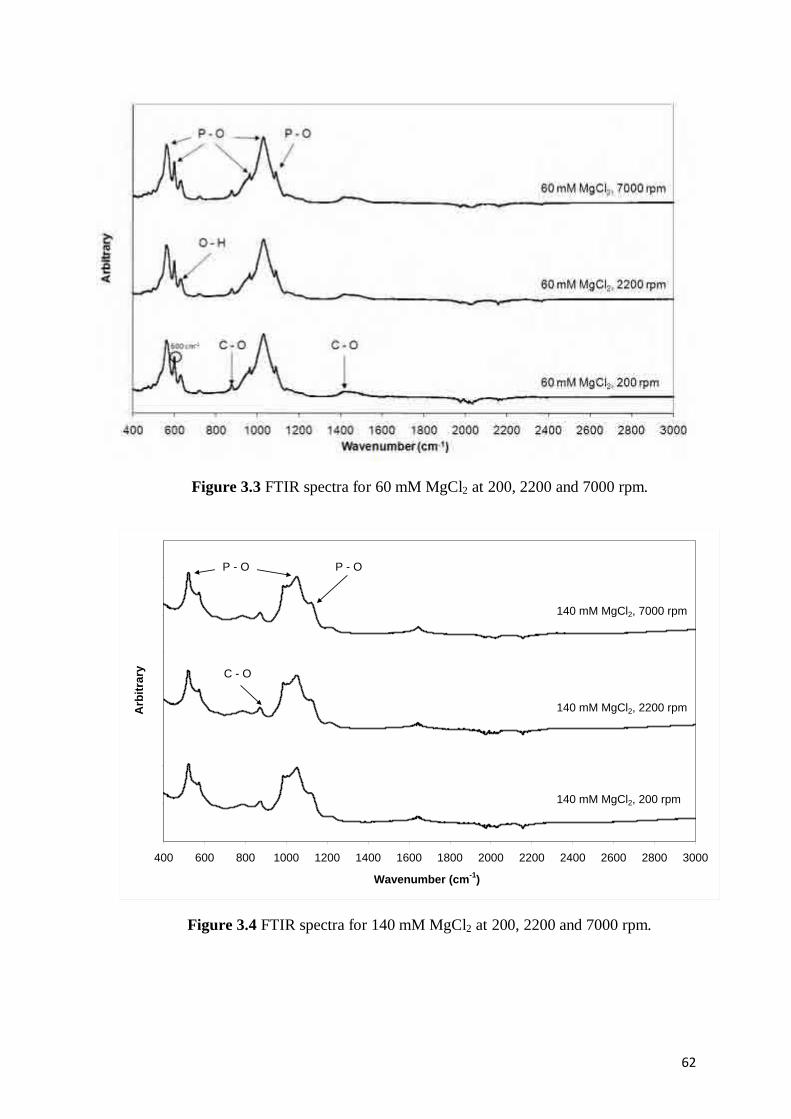
62
Figure 3.3 FTIR spectra for 60 mM MgCl2 at 200, 2200 and 7000 rpm.
0.4
0.6
0.8
1
1.2
1.4
1.6
1.8
2
400 600 800 1000 1200 1400 1600 1800 2000 2200 2400 2600 2800 3000
Wavenumber (cm-1
)
Arb
itra
ry
140 mM MgCl2, 200 rpm
140 mM MgCl2, 2200 rpm
140 mM MgCl2, 7000 rpm
P - O
C - O
P - O
Figure 3.4 FTIR spectra for 140 mM MgCl2 at 200, 2200 and 7000 rpm.

63
3.4.2 X-ray Diffraction (XRD)
3.4.2.1 Hydroxyapatite - sintered
The formation of hydroxyapatite was indicated by the characteristic peak occurring at 2θ =
31.8o which appeared on all of the HAp samples [Shimbayashi et al. (2000)] and was verified
by the pattern for HAp from the JCPDS catalogue. The narrow peaks in the XRD spectra
indicate a high degree of crystallinity in the hydroxyapatite particles (an average of 63 %
calculated by equation 2). After sintering at 600 oC, no other phase besides hydroxyapatite
was identified. The XRD patterns obtained for all of the HAp samples showed that they are
all the same, whereby processing conditions does not effect on the resultant phase. XRD data
for some HAp samples prepared at various agitation rates at 20 oC and 40
oC are shown in
Figures 3.5 and 3.6, respectively.
0
500
1000
1500
2000
2500
3000
3500
4000
4500
5000
20 25 30 35 40 45 50 55 60 65 70 75 80
2θ (o)
Arb
itra
ry
200 rpm at 20 oC
1200 rpm at 20 oC
2200 rpm at 20 oC
3000 rpm at 20 oC
5000 rpm at 20 oC
7000 rpm at 20 oC
HAp
Figure 3.5 XRD patterns for some of HAp samples produced at 20 oC.

64
0
500
1000
1500
2000
2500
3000
3500
4000
4500
5000
20 25 30 35 40 45 50 55 60 65 70 75 80
2θ (o)
Arb
itra
ry
200 rpm at 40 oC
1200 rpm at 40 oC
2200 rpm at 40 oC
3000 rpm at 40 oC
5000 rpm at 40 oC
7000 rpm at 40 oC
HAp
Figure 3.6 XRD patterns for some of HAp samples produced at 40 oC.
3.4.2.2 Mg intercalated calcium phosphate - sintered
XRD analysis of HAp-Mg intercalated particles did not show any detectable evidence of Mg
for the 20 to 40 mM concentrations. It has been reported that the addition of MgCl2 at these
concentrations will not change significantly the Ca/P ratio of the hydroxyapatite composition;
the Ca:P ratio is equal to 1.64 for 20 mM and 1.57 for 40 mM [Chowdhury et al. (2004)].
Only when 60 mM MgCl2 was added the Ca/P ratio changed to 1.29 and showed the
characteristic peak for octacalcium phosphate (OCP) [Ca4-x-Mgx(PO4)3] at 21o. At 140 mM
MgCl2 addition hydroxyapatite is transformed to OCP as evidenced by the intensity of the 21o
peak, with a Ca/P ratio of 1.17. XRD data of some of the HAp-Mg samples are shown in
Figure 3.7.

65
Figure 3.7 XRD patterns of hydroxyapatite samples prepared with 0 mM, 20 mM, 80 mM
and 140 mM MgCl2 at 2200 rpm and 20 oC.
3.4.2.3 Hydroxyapatite- pre-sintered
XRD analysis of pre-sintered HAp particles shows that the Ca/P formed was calcium nitrate
before being reverted to hydroxyapatite upon sintering. XRD data of a pre-sintered HAp
sample are shown in Figure 3.8.

66
0
200
400
600
800
1000
1200
20 25 30 35 40 45 50 55 60 65 70 75 80
2θ (o)
Arb
itra
ry
Pre-sintered material
Calcium nitrate
Figure 3.8 XRD spectra of a pre-sintered HAp sample produced at 1200 rpm and 20 oC.
3.4.3 Scanning Electron Microscopy (SEM)
Prior to sintering HAp shows a plate-like morphology approximately 50 x 20 µm as seen in
Figure 3.9. Fathi et al. [Fathi et al. (2008)] reported 200 µm agglomerated particles sizes
before sintering, but the lack of process agitation rate details makes it difficult to make a
comparison. Meanwhile, prior to sintering HAp-Mg shows a flower-like morphology as seen
in Figure 3.10.

67
Figure 3.9 SEM of pre-sintered HAp particles produced at 2200 rpm and 20 oC.
Figure 3.10 SEM of pre-sintered intercalated HAp-Mg particles produced using 140 mM
MgCl2. The crystallinity decreased slightly from 63% without MgCl2 to 58% (as calculated
from Equation 3.2) when 140 mM was added.
Typical SEMs of post-sintered HAp nanoparticles are shown in Figure 3.11. It can be seen
that the fully processed particles form agglomerates of approximately <1 to 5 µm with no
obvious difference in morphologies.

68
(a) 200 rpm 20 oC (b) 200 rpm 40 oC
(c) 1200 rpm 20 oC (d) 1200 rpm 20 oC
(e) 2200 rpm 20 oC (f) 2200 rpm 40 oC
(g) 3000 rpm 20 oC (h) 3000 rpm 40 oC

69
Figure 3.11 SEM images of HAp after processing at different agitation rates and
temperatures.
3.4.4 Transmission Electron Microscope (TEM)
Table 3.1 and 3.2 shows TEMs of post-sintered HAp particles obtained from processing with
the overhead stirrer and homogeniser, respectively. The mean size range of the particles
obtained is between 43 and 68 nm. The particles are generally cuboid-like at lower rpm with
the overhead stirrer (images in Table 3.1; while particles with an elongated ellipse-like
morphology were obtained at higher rpm with the homogeniser (images in Table 3.2). (Note,
the equivalent particle diameter was used for the non-uniform particles obtained at higher
agitation rates). This behaviour can be explained by the shear produced by the agitation
equipment. The overhead stirrer and homogeniser operate on similar concepts in that they
both induce shear into the fluid. The homogeniser is a mechanical blade-type and at high rpm
would have induced high shear in the mixing zone, creating a vortex which built up
aggressive flow behaviour within the system. The Rushton turbine impeller attached to the
overhead stirrer would have also produced shear but at a lower level as a result of less energy
(i) 7000 rpm 20 oC (j) 7000 rpm 40 oC

70
input at the lower rpm. At high rpm, the high energy dissipation would lead to increased
nucleation rates, which would lead to smaller particles, and at the same time affect
mechanism of crystal growth and the subsequent morphology [Ding et al. (2008)].
Feng et al. (2005) used TEM images to report average HAp particle diameters between 10 to
15 nm with an ellipse-like morphology. Fathi et al. (2007 & 2008) also reported an ellipse-
like morphology with particle sizes between 20 to 35 nm that were dependent on the aging
duration and sintering temperature. Particle sizing was also carried out from XRD analyses in
conjunction with Scherrer’s formula and the sizes are also reported in Table 3.1 and 3.2. Fathi
et al. (2007 & 2008) used this method to estimate the primary size of particles and then
corroborated their calculations with TEM images. However, neither Feng nor Fathi’s paper
mentioned the type of agitator and the agitation rate used. In a similar light, Krajewski et al.
(2005) produced carbonated hydroxyapatite particles, however they have not shown TEM
images of their particles to enable a comparison to be made. The particle sizes of 43 to 68 nm
seen in the TEM images above compare well with those of Fathi et al. (2007) and signify the
grain particle size.

71
Stirring
Temp.200 rpm 800 rpm 1200 rpm 1800 rpm 2200 rpm
20 oC
Particle Size
TEM
64 ± 8 nm
Scherrer’s
56 nm
TEM
61 ± 7 nm
Scherrer’s
53 nm
TEM
60 ± 9 nm
Scherrer’s
49 nm
TEM
57 ± 5 nm
Scherrer’s
48 nm
TEM
54 ± 6 nm
Scherrer’s
45 nm
40 oC
Particle Size
TEM
68 ± 9 nm
Scherrer’s
54 nm
TEM
63 ± 6 nm
Scherrer’s
53 nm
TEM
61 ± 8 nm
Scherrer’s
50 nm
TEM
57 ± 8 nm
Scherrer’s
48 nm
TEM
56 ± 8 nm
Scherrer’s
46 nm
Table 3.1 TEM images and particle size estimations based upon the images and Scherrer’s formula (Eqn. 1) for HAp samples produced with the overhead stirrer.

72
Stirring
Temp.3000 rpm 4000 rpm 5000 rpm 6000 rpm 7000 rpm
20 oC
Particle Size
TEM
47 ± 5 nm
Scherrer’s
41 nm
TEM
60 ± 9 nm
Scherrer’s
50 nm
TEM
54 ± 6 nm
Scherrer’s
45 nm
TEM
47 ± 5nm
Scherrer’s
41 nm
TEM
43 ± 4 nm
Scherrer’s
38 nm
40 oC
Particle Size
TEM
52 ± 6 nm
Scherrer’s
45 nm
TEM
61± 8 nm
Scherrer’s
49 nm
TEM
56 ± 8 nm
Scherrer’s
46 nm
TEM
52 ± 6nm
Scherrer’s
45 nm
TEM
45 ± 5 nm
Scherrer’s
39 nm
Table 3.2 TEM images and particle size estimations based upon the images and Scherrer’s formula (Eqn. 1) for HAp samples produced with the homogenizer.

73
3.4.5 Dynamic Light Scattering (DLS)
Particle sizing measurements by DLS was undertaken for all HAp samples for both reaction
temperatures and are shown in Table 3.3 (unfiltered) and Table 3.4 (filtered). Generally it can
be observed that a lower agitation rate led to larger sized agglomerates. Samples were
sonicated for one hour to disperse the particles prior to DLS measurements. Sonication is a
commonly used technique to disperse agglomerates, as it can pull the liquid apart to form
evacuated cavities. The formation and destruction of these cavities can impose a shear force
on agglomerates, capable of overcoming the van der Waals force holding them together.
Simultaneously, cavity formation and destruction can also enhance agglomeration in the
liquid by promoting interactions and contact of particles by kinetic coagulation. The DLS
measurements showed a disparity in the particle size compared to the sizes seen in the SEM
images (Figure 3.10). Average values between 145 to 219 nm (P<0.05) were obtained and
indicated that kinetic coagulation had occurred as the particle size could not be further
reduced by sonication. The polydispersity indice (PDI) values for the filtered samples (0.108
to 0.167) indicate that the particles formed as agglomerates and that a single species is not
present, which reflected in the microscopic images. A near-monodisperse system would have
a PDI value of 0.1 or lower, which the filtered samples are close to this value. In the
unfiltered samples, the particles aggregated to form agglomerates. The filtered samples
resulted in smaller particles but the PDI values still implied that aggregation of the primary
particles had occurred but to less extent. Filtering removes larger agglomerates and this leads
to small size fraction of the HAp particles.

74
*standard deviation of the mean for 3 batches with 3 replicates for each batch
Table 3.3 Particle size measurement by DLS (unfiltered).
Stirring rate (rpm) Temperature (oC) Particle Size by DLS *(nm) PDI
200
20 372 ± 18 0.249
40 405 ± 13 0.269
400
20 531 ± 14 0.276
40 473 ± 15 0.256
800
20 384 ± 17 0.253
40 427 ± 16 0.233
1000
20 533 ± 16 0.245
40 386 ± 15 0.232
1200
20 352 ± 22 0.251
40 426 ± 16 0.231
1400
20 502 ± 20 0.254
40 465 ± 15 0.243
1800
20 512 ± 16 0.234
40 467 ± 18 0.265
2000
20 431 ± 15 0.253
40 535 ± 16 0.231
2200
20 496 ± 12 0.235
40 465 ± 17 0.256
3000
20 376 ± 19 0.238
40 432 ± 16 0.245
4000
20 408 ± 13 0.250
40 503 ± 16 0.217
6000
20 390 ± 16 0.245
40 453 ± 18 0.256
7000
20 465 ± 13 0.275
40 488 ± 17 0.265
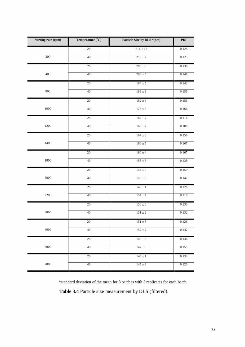
75
*standard deviation of the mean for 3 batches with 3 replicates for each batch
Table 3.4 Particle size measurement by DLS (filtered).
Stirring rate (rpm) Temperature (oC) Particle Size by DLS *(nm) PDI
200
20 211 ± 12 0.128
40 219 ± 7 0.125
400
20 203 ± 8 0.136
40 206 ± 5 0.146
800
20 184 ± 5 0.143
40 182 ± 3 0.155
1000
20 182 ± 6 0.156
40 178 ± 5 0.164
1200
20 162 ± 7 0.114
40 166 ± 7 0.108
1400
20 164 ± 3 0.156
40 166 ± 5 0.167
1800
20 160 ± 4 0.167
40 156 ± 6 0.138
2000
20 154 ± 5 0.159
40 153 ± 6 0.147
2200
20 148 ± 1 0.126
40 154 ± 4 0.118
3000
20 150 ± 6 0.130
40 151 ± 2 0.132
4000
20 151 ± 3 0.126
40 152 ± 2 0.142
6000
20 146 ± 5 0.136
40 147 ± 6 0.155
7000
20 145 ± 1 0.133
40 145 ± 3 0.120

76
The particle size estimations by Scherrer’s formula are much more comparable to those
observed in the TEM images, whereas the DLS measurements gave the sizes of agglomerated
particles and not of the primary nanoparticles.
3.4.6 Effect of agitation rate on particle size
The Power number (Np) is a useful parameter to determine the power required for agitation,
whereas the Reynolds number (Re) is used to characterise the flow regimes in a stirred tank,
which are either laminar (Re < 2000), turbulent (Re > 10,000) or transitional flow (Re 2000 –
10,000) [Ding et al. (2008)]. Both the Power number and Reynolds number vary with
agitation rate. The Power number is given by:
Power Number = 53Dn
PNp
Equation 3.3
where, P is power (W), ρ is ethanol density (kg m-3
), n is rotational speed (rpm 60-1
) and D is
the diameter of the impeller (0.05 m for the overhead stirrer and 0.019 m for the
homogeniser). The values of Np were obtained from power curve correlations given in
references by Ding et al. (2008) and Sinnott for the two agitators based on the respective Re
numbers. 0.4 was used for the Rushton turbine and 4.5 for the homogenizer.
The impeller Reynolds number is given by:
2
ReND
Equation 3.4
where ρ is ethanol density (kg m-3
), N is rotational speed (rpm 60-1
), D is the diameter of
impeller (dimensions as Equation 3) and µ is ethanol viscosity (kg m-1
s-1
). The densities and
viscosities of ethanol at the temperature conditions were obtained from the literature [Paul et
al. (2004)]. The relationship between power and particle size and Re number and particle size

77
for the two particle sizing methods (TEM and DLS) at 20 oC and 40
oC are shown in Figures
3.12 and 3.13, respectively.
20
60
100
140
180
220
260
0 2 4 6 8 10 12 14
Power, P (W)
Pa
rtic
le s
ize
(n
m)
DLS 20 oC DLS 40 oC TEM 20 oC TEM 40 oC
7000
rpm
3000
rpm
2200
rpm
1200
rpm
200
rpm
DLS
TEM
Figure 3.12 Effect of Power on Particle size (nm) at 20 oC and 40
oC.
20
60
100
140
180
220
260
0 50000 100000 150000 200000
Reynolds number, Re
Part
icle
siz
e (
nm
)
DLS 20 oC DLS 40 oC TEM 20 oC TEM 40 oC
200
rpm
1200
rpm 2200
rpm
3000
rpm
7000
rpm
DLS
TEM
Figure 3.13 Influence of Re Numbers on Particle size (nm) at 20 oC and 40
oC.

78
It can be seen that for all particle sizing methods higher power resulted in smaller particle
sizes. A similar trend is seen for the effect of Re number on particle size. As the power
increases the energy introduced into the system would affect the kinetics of nuclei
aggregation leading to the formation of smaller particles. At lower Re values, there is less
inertia force accumulating in the system. At higher Re numbers there is high energy
dissipation and turbulence in the mixing zone, which would lead to increased nucleation rate
and also the break-up of larger aggregates into smaller secondary aggregates as evidenced by
the decreased sizes for the respective TEM and DLS data [Lange (1967)]. It can be seen from
Figure 3.13 and Table 3.4 that the agitation rate has an influence upon the filtered
agglomerate size obtained by DLS until higher agitation rates (>2200 rpm) and Re numbers
(turbulence) are reached. Around this rpm it can be inferred that kinetic coagulation occurred,
which led to the formation of stable aggregates and therefore particle size tends to become
less dependent on agitation rate.
The effect of agitation rate on primary particle size can be seen by comparing the TEM sizing
results at 200 rpm and 7000 rpm for both temperatures (see Table 3.1 and 3.2 and Figure
3.13). It can be seen that the primary particle size decreased steadily with an increase in
agitation rate. While gentle agitation causes nucleation in solutions that are otherwise stable,
increased agitation creates an even greater tendency to form secondary nuclei [Pacek et al.
(2007)] and would explain the reduction in the primary particle size over the agitation rates
studied.

79
3.4.7 Effect of temperature
Lower temperatures are known to influence the rate of growth and size of crystals through its
effect on supersaturation [Mullin (1960 & 2000), Myerson & Ginde (1993), Jones & Mullin
(1974)]. In this work, both TEM and DLS data (see Tables 3.1, 3.2 and 3.4) show very small
differences for both the agglomerated and primary particle sizes obtained at 20 and 40 oC,
with slightly larger sizes being obtained at higher temperature. On one hand, higher
temperature would lead to a decrease in solution viscosity which would accelerate the
collision rate of nuclei and therefore lead to smaller particles, however at 40 oC a higher
collision rate may have also led to increased probability of coalescence and the observed
small increase in particle size [Cheng & Li (2009)]. The temperature has less effect on the
agglomerate sizes obtained by DLS at higher rpm. This can be attributed to the formation of
stable aggregates in the mixing zone.
3.4.8 Effect of Mg2+
on HAp particle size
The effect of incorporating Mg2+
ions into the HAp nanoparticles has been reported to
transform larger particles (2500 to 500 nm) to more smaller particles of 100 to 500 nm as a
result of varying the concentration of the Mg2+
and precipitation rate [Chowdhury et al.
(2004)]. Chowdhury et al. (2004) have produced Ca-Mg hydroxyapatite particles
approximately between 100 to 500 nm depending on the Mg fraction. In a similar light,
Miyaji et al. (2005) have produced zinc-substituted calcium hydroxyapatite between
approximately 200 to 1100 nm depending on the Zn fraction, and Krajewski et al. (2005)
have reported carbonated hydroxyapatites, though particle sizes were not given. In this
chapter a series of experiments were undertaken to study the effects of agitation rate and

80
magnesium concentrations on particle size using the sol gel technique at 20 oC and therefore
extended the work of Chowdhury et al. (2004).
Post sintering the primary particles exhibited similar morphologies to those of HAp particles
over the range of agitation rates. TEM and filtered DLS particle size data obtained at different
agitation rates and magnesium concentrations are shown in Figure 3.14. As for HAp particles,
an increase in agitation rate also led to a decrease in the primary particle and agglomerate
sizes for the reasons discussed earlier. In general, the primary particle and agglomerate sizes
decreased with higher concentrations of MgCl2. The inhibitory effect of Mg2+
on particle
growth creates a distorted atomic structure within the hydroxyapatite due to the replacement
of Ca2+
with Mg2+
, which subsequently slows the growth of the particles [Miyaji et al.
(2005)] and results in the smaller particle sizes. The relatively smaller ionic radius of the
Mg2+
ions (0.65 Å) compared to the Ca2+
ions (0.99 Å) [Blumenthal (1989)], could further
contribute to the effect on the HAp particle size. At higher MgCl2 concentrations (60 to 140
mM) the particle size became less dependent on concentration for agitation rates above 2200
rpm due to the stronger influence of agitation rate over concentration.

81
140
150
160
170
180
190
200
210
220
200 1200 2200 3000 7000
Stirring rate (rpm)
Pa
rtic
le s
ize
(n
m)
0.0 mM MgCl2 20 mM MgCl2 40 mM MgCl2 60 mM MgCl2 140 mM MgCl2
DLS
Stirring rate (rpm)
40
45
50
55
60
65
70
75
80
200 1200 2200 3000 7000
Stirring rate (rpm)
Pa
rtic
le s
ize
(n
m)
0.0 mM MgCl2 0.0 mM MgCl2 20 mM MgCl2 40 mM MgCl2 60 mM MgCl2 140 mM MgCl2
TEM
Figure 3.14 Effect of Mg2+
intercalation on HAp particle size for different MgCl2
concentrations and agitation rates at 20 oC.

82
3.5 Conclusions
The effect of process conditions on the particle size of HAp and intercalated HAp-Mg
particles are reported. It can be concluded that the primary particle size for both HAp and
HAp-Mg particles decreased with higher agitation rates and can be explained in terms of the
power input and turbulence within the mixing zone influencing the nucleation rate. At higher
agitation rates the filtered DLS data showed the formation of stable agglomerates above 2200
rpm as the agitation rate did not significantly affect the particle size. An increase in
temperature from 20 to 40 oC had a slight effect on particle size. The intercalation of Mg into
the HAp structure led to a decrease in particle size with increased MgCl2 concentration and
increased agitation rate, although this became less significant at agitation rates above 2200
rpm. Different particle morphologies can be obtained at different agitation rates, which are
dependant on equipment selection. Cuboid-like particles were obtained at lower agitation
rates with the overhead stirrer while elongated particles can be obtained at higher agitation
rate using the homogeniser.

83
3.6 References:
Balamurugan, A. Rebelo, A. H. S. Lemos, A. F. Rocha, J. H. G. Ventura, J. M. G. Ferreira, J.
M. F. 2008. Suitability evaluation of sol-gel derived Si-substituted hydroxyapatite for dental
and maxillofacial applications through in vitro osteoblasts response. Dental Materials 24:
1374 – 1380.
Bigi, A. Falini, G. Foresti, E. Gazzano, M. Ripamonti, A. Roveri, N. 1993. Magnesium
influence on hydroxyapatite crystallization, J. Inorg. Biochem 49: 69 – 78.
Blumenthal, N. C. 1989. Mechanisms of inhibition of calcification. Clin. Orthop. 247: 279 –
289.
Cheng, W. Li, Z. 2009. Precipitation of nesquehonite from homogeneous supersaturated
solutions. Cryst. Res. Technol., 44: 937 – 947.
Chowdhury, E. H. Kunou, M. Nagaoka, M. Kundu, A. K. Hoshiba, T. Akaike, T. 2004. High-
efficiency gene delivery for expression in mammalian cells by nanoprecipitates of Ca-Mg
phosphate. Gene 341: 77 – 82.
Deppert, W. R. Lukacin, R. 1999. Chapter 5 Hydroxyapatite Chromatography. Protein Liquid
Chromatography 271 – 299.
Ding, P. Pacek, A. W. 2008. De-agglomeration of goethite nano-particles using ultrasonic
comminution device. Powder Technology, 187: 1 -10.
Epple, M. Sokolova, V. 2008. Inorganic Nanoparticles as Carriers of Nucleic Acids into
Cells. Angew. Chem. Int. Ed. 47: 1382 – 1395.
Fadeev, I. V. Shvorneva, L. I. Barinov, S. M. Orlovskii, V. P. 2003. Synthesis and structure
of magnesium-substituted hydroxyapatite, Inorg. Mater., 39 (9): 947 – 950.
Fathi, M. H. Hanifi, A. 2007. Evaluation and characterization of nanostructure
hydroxyapatite powder prepared by simple sol-gel method. Materials Letters 61: 3978 –
3983.
Fathi, M. H. Hanifi, A. Mortazavi, V. 2008. Preparation and bioactivity evaluation of bone-
like hydroxyapatite nanopowder. Journal of Materials Processing Technology 202: 536 –
542.
Feng, W. Mu-sen, L. Yu-peng, L. Yong-xin, Q. 2005. A simple sol-gel technique for
preparing hydroxyapatite nanopowders, Materials Letters 59: 916 – 919.
Feng, Y. Haifeng, G. Haijiao, Z. Xiulan, H. 2010. Polymeric micelle-templated synthesis of
hydroxyapatite hollow nanoparticles for a drug delivery system. Acta Biomaterialia 6: 2212 –
2218.
Hannay, J. B. Hogarth, J. 1879. On the solubility of solids in gases. Proc. Roy. Sec. (London)
29: 324.

84
Ichiro, O. Toshiharu, Y. Hai-Ying, J. Yoshinori, I. Hirobumi, H. Yoshikiyo, A. Masanori, N.
Tetsunori, O. Kowichi, J. 2004. Combination of porous hydroxyapatite and cationic
liposomes as a vector for BMP-2 gene therapy. Biomaterials 25: 4709 – 4718.
Jenkins, R. Synder, R. L. 1996. Introduction to X-ray Powder Diffractometry. John Wiley
and Sons: New York.
Jones, A. G. Mullin, J. W. 1974. Programmed cooling crystallization of potassium sulphate
solutions. Chem. Eng. Sci. 29: 105 – 118.
Kannan, S. Lemos, I. A. F. Rocha, J. H. G. Ferreira, J. M. F. 2005. Synthesis and
characterisation of magnesium substituted biphasic mixtures of controlled hydroxyapatite/β-
tricalcium phosphate ratios. J. Solid State Chem. 178: 3190 – 3196.
Kano, J. Zhang, Q. Saito, F. Baron, M. Nzihou, A. 2006. Synthesis of hydroxyapatite with the
mechanochemical treatment products of PVC and CaO. Process Safety and Environmental
Protection 84: 309 – 312.
Kawata, M. Uchida, H. Itatani, K. Okada, I. Koda, S. Aizawa, M. 2004. Development of
porous ceramics with well-controlled porosites and pore sizes from apatite fibers and their
evaluations. J. Mater. Sci. Mater. Med. 817 – 823.
Krajewski, A. Mazzocchi, M. Buldini, P. L. Ravaglioli, A. Tinti, A. Taddei, P. Fagnano, C.
2005. Synthesis of carbonated hydroxyapatites: efficiency of the substitution and critical
evaluation of analytical methods. Journal of Molecular Structure, 744 – 747: 221 – 228.
Landi, E. Tampieri, A. Celotti, G. Sprio, S. 2000. Densification behaviour and mechanisms of
synthetic hydroxyapatites. J. Eur. Ceram. Soc. 20: 2377 – 2387.
Lange’s Handbook of Chemistry 1967. 10th Ed. McGraw-Hill, New York.
Lim, G. K. Wang, J. Ng, S. C. Gan, L. M. 1999. Nanosized hydroxyapatite powders from
microemulsions and emulsions stabilised by a biodegradable surfactant. J. Mater. Chem. 9:
1635.
Miyaji, F. Kono, Y. Suyama, Y. 2005. Formation and structure of zinc-substituted calcium
hydroxyapatite. Mater. Res. Bull. 40: 209 – 213.
Molle, P. Lienard, A. Gramsik, A. 2005. Apatite as an interesting seed to remove phosphorus
from waste-water in constructed wetlands. Water Sci. Technol. 51:193 – 203.
Mullin, J. W. Raven, K. D. 1960. Nucleation in agitated solutions. Nature, 190:251.
Mullin, J. W. 2000. Crystallization. Oxford, UK: Butterworth-Heinemann.
Myerson, A. S. Ginde, R. 1993. Crystals, crystal growth and nucleation. In: Handbook of
Industrial Crystallization. St. Louis, MO: Butterworth-Heinemann; 33 – 63.

85
Ni, G. X. Lu, W. W. Xu, B. Chiu, K. Y. Yang, C. Li, Z. Y. Lam, W. M. Luk, K. D. K. 2006.
Interfacial behaviour of strontium-containing hydroxyapatite cement with cancellous and
cortical bone. Biomaterials 27:5127 – 5133.
Pacek, A. W. Ding, P. Utomo, A. T. 2007. Effect of energy density, pH and temperature on
de-aggregation in nano-particles/water suspensions in high shear mixer. Powder Technology
173: 203 – 210.
Paul, E. L. Atiemo-Obeng, V. A. Kresta, S. M. 2004. Handbook of Industrial Mixing. Wiley-
Interscience.
Pons, M-N. Vivier, H. Delcour, V. Authelin, J-R. Paillères-Hubert, L. 2002. Morphological
analysis of pharmaceutical powders. Powder Tech. 128: 276-286.
Rodriquez-Clemente, R. Lopez-Macipe, A. Gomez-Morales, J. Torrent-Burgues, J. Castano,
V. M. 1998. Hydroxyapatite precipitation: A case of nucleation-aggregation-agglomeration-
growth mechanishm. J. Eur. Ceram. Soc. 18: 1351 – 1356.
Shimbayashi, S. Hashimoto, N. Kawamura, H. Uno, T. Mineral Scale Formation and
Inhibition. In: Amjad, Z (Ed.), Plenum Press: New York, 14 – 15.
Sinnott, R. K. Coulson & Richardson’s Chemical Engineering. Volume 6: Chemical
Engineering Design, 4th ed. (Butterworth – Heinemann), 473 – 474.
Suchanek, W. L. Byrappa, K. Shuk, P. Riman, R. E. Janas, V. F. TenHuisen, K. S. 2004.
Preparation of magnesium-substituted hydroxyapatite powders by the mechanochemical-
hydrothermal method. Biomaterials 25: 4647 – 4657.
Tas, A. C. 2000. Combustion synthesis of calcium phosphate bioceramic powders. J. Eur.
Ceram. Soc. 20: 2389.
Varma, H. Babu, S. S. 2005. Synthesis of calcium phosphate bioceramics by citrate gel
pyrolysis method. Ceram. Int. 31: 109 – 114.
Weng, W. J. Baptista, J. L. 1997. A new synthesis of hydroxyapatite. J. Eur. Ceram. Soc. 17:
1151-1156.
Yoshmura, M. Suda, H. Okmoto, K. Loku, K. 1994. Hydrothermal synthesis of
biocompatible whiskers. J. Mater. Sci. 29: 3399.

86
4.0 Hydroxyapatite (HAp) prepared by Anti-solvent processing
4.1 Introduction
Supercritical fluid (SCF) technology has found its place in many industrial applications, such
as nanoparticle fabrication, food processing (decaffeination of coffee beans as an example),
chemical manufacturing, extraction, dry cleaning, polymer processing, waste treatment and
particle coating [Palakodaty et al. (2002), Adschiri & Arai (2002), Hay & Khan (2002)]. It is
chosen as an alternative processing method, as it can avoid the use of harsh and toxic organic
solvent. SCF technology, specifically supercritical carbon dioxide (scCO2) is considered a
‘green technology’, as CO2 is benign, environmentally friendly, a GRAS solvent, easily
available and recyclable [DeSimone (2002)].
SCF technology can be applied to the manufacture of nanoparticles for advanced drug
delivery and drug formulations systems. The particles once formed need not undergo further
processing or treatment and this feature makes SCF technology amenable to process
biomolecules and other sensitive compounds in their native pure state [Chattopadhyay &
Gupta (2002)]. There are many routes to produce particles by scCO2; these include for
example, Rapid Expansion of Supercritical Solutions (RESS), Gas Anti-Solvent precipitation
(GAS), Precipitation from Compressed Antisolvent (PCA), Supercritical Antisolvent process
(SAS), and Solution Enhanced Dispersion by Supercritical fluids (SEDS), the process
selection depends on the solubility of the active compound in scCO2 [Byrappa et al. (2008)].
In this section, HAp formed from the wet chemistry method is recrystallised by SCF
processing using GAS and SEDS methods in order to evaluate the potential of SCF in
producing HAp particles. The selection of the GAS method is based on the simplest method
of all of the SCF methods, while for the SEDS method has been selected in order to evaluate

87
the effect of rapid supersaturation and solvent removal on particle formation. The
recrystallised particles produced were then characterised by Fourier Transform Infrared
Spectroscopy (FTIR), X-ray Diffraction (XRD), High Performance Particle Sizer (HPPS),
Scanning Electron Microscopy (SEM) and Transmission Electron Microscopy (TEM).
4.1.1 SCF methods selection
4.1.1.1 Gas Anti-Solvent (GAS) method
Gallagher [Gallagher et al. (1989 & 1992)] first reported using this technique in the
recrystallisation of explosive substances of nitroguanidine & cyclotrimethylenetrinitramine
(RDX). Generally, in the GAS method, the target active is dissolved in a suitable organic
solvent. Adding scCO2 as an antisolvent expands the organic solution causing a reduction of
the organic solvent power which leads to the supersaturation of the solution. The particles of
the active solute are formed as the active losses its affinity in the organic solvent. The solvent
expanded with the scCO2 antisolvent is purged, and the produced particles are washed with
additional scCO2 to remove remaining organic solvent. The principle of the antisolvent
process is based on a rapid decrease in the solubilisation power of a solvent by addition of a
second fluid as antisolvent. Particle size distribution can be controlled by adjusting the values
of temperature, pressure and composition [Mishima (2008)]. The main disadvantage of the
GAS precipitation process is the difficulty to remove the remaining solvent completely
because the process is carried out in a batch process. An additional wash-out treatment with
scCO2 may be required for the production of a pharmaceutical product on an industrial scale.
The schematic diagram of the GAS rig is shown in Figure 4.1. The method of this technique
is given in detail in section 4.2.1.1.

88
Figure 4.1 Schematic diagram of the GAS rig.

89
4.1.1.2 Solution Enhanced Dispersion by Supercritical fluids (SEDS) method
The chief developers of SEDSTM
, Bradford University, have successfully applied the process
to numerous situations, including processing of dyes [Hanna (1994)], lactose [Hanna (1995)]
and polystyrene [Hanna (1998)]. Other workers have successfully manufactured proteins of a
smaller and more uniform nature than conventional techniques [Sloan et al. (1998)]. The
major success of SEDSTM
is in the production of intrapulmonary delivery systems, where the
particle size needs to be small (<5 μm) but the distribution needs to be very tight. In the
SEDS method, particle formation is initiated by the mass transfer of the supercritical fluid
into the sprayed droplet and by the rate of solvent transfer into the supercritical phase. In
particular, a high mass transfer allows a faster nucleation and a smaller particle size with less
agglomeration [Palakodaty et al. (1998)]. The schematic diagram of the SEDS rig and its
coaxial nozzle diagram are shown in Figure 4.2 and 4.3 respectively. The method of this
technique is given in detail in section 4.2.1.2.

90
Figure 4.2 Schematic diagram of the SEDS rig.
DMSO containing HAp
Supercritical CO2
Mixing chamber
Particle formation
Figure 4.3 The SEDS coaxial nozzle diagram used in this work.

91
4.1.2 Solvent selection
4.1.2.1 Classes of solvents
Solvents and solutes can be broadly classified into polar (hydrophilic) and non-polar
(hydrophobic). The polarity can be measured as the relative permittivity or the dipole
moment of a compound. The polarity of a solvent determines the type of compounds it is able
to dissolve and with which other solvents or liquid compounds it is miscible. As a rule of
thumb, polar solvents best dissolve polar compounds and non-polar solvents best dissolve
non-polar compounds, i.e. ‘like dissolves like’. The Hildebrand solubility parameter is a
useful approach for evaluating the solubility of a compound in another [Goodarzi et al.
(2010)]. The solubility parameter is a numerical value that indicates the relative solvency of a
specific solvent. It is derived from the cohesive energy density of the solvent, which in turn is
derived from the heat of vaporisation. Polar solvents can be classified into two categories,
which are the polar aprotic solvents (cannot donate hydrogen bonds, but have high dielectric
constants and high polarity) and the polar protic solvents (can participate in hydrogen
bonding and contains dissociable H+).
4.1.2.2 Solvent screening
Solvent screening was done in this study as to select a solvent which not only dissolves HAp
but is also compatible with supercritical CO2. In total, 26 solvents were screened. The non-
polar solvents tested were benzene, chloroform, cyclohexane, dichloromethane, diethyl ether,
ethyl acetate, heptane, hexane and methyl cyclohexane. The polar aprotic solvents tested
were 1,4 – dioxane, acetone, acetonitrile, dimethyl formamide (DMF), dimethyl sulfoxide
(DMSO), ethyl acetate, isopropyl acetate, methyl ethyl ketone (MEK), N-methyl 2-

92
pyrrolidone (NMP) and tetrahydrofuran (THF). The polar protic solvents tested were n-
butanol, ethanol, isopropanol, methanol, n-propanol, octanol and water.
Solvent screening in this study is based on the solubility of phosphate determined by
spectrophotometry. The phosphate dissolved in a solvent was complexed with molybdate-
vanadate reagent and its quantity calculated photometrically at 400 nm. The obtained
absorbance was then compared with a standard phosphate calibration curve with known
amount of phosphate. An amount of 0.1 mg, 0.5 mg, 1.0 mg, 1.5 mg and 2.0 mg of HAp were
dissolved in 100 ml of respective solvent that was tested. The solution was then filtered and
complexed with molybdate-vanadate until the colour of the solution turned yellow. The
calculation of HAp solubility is shown in Chapter 4 Appendix (Appendix 4 A).
HAp is an inorganic and ionic compound. Therefore, it will not dissolve in non-polar
solvents, as these solvents do not provide the polarity for the interactions of ions between the
solvent and the solute. This was further proven by the insolubilities of any amount of HAp in
the non-polar solvents. HAp can easily be dissolved in acidic solution such as acetic acid and
formic acid, but the use of these acids is not suitable for the supercritical processing due to
their extremely low solubilities in the CO2 antisolvent. Furthermore, these acids will damage
some parts of the supercritical rig which consisted of plastic parts such as the pump tubing,
pipings and ‘o’ ring seals. For the polar aprotic solvents, only DMF and DMSO showed that
HAp can be soluble with an amount of 2 mg/l and 3 mg/l respectively. However, due to the
toxicity of DMF, this solvent was omitted. Lastly, for the polar protic solvents, an amount of
6 mg/l of HAp can be solubilised in water. Due to the low solubility of water in supercritical
CO2, water will not be used as a solvent in the supercritical processings.
93
4.1.2.3 Dimethyl sulfoxide (DMSO)
Dimethyl sulfoxide (DMSO) is a chemical compound with the formula of (CH3)2SO. It is a
colourless liquid and is a polar aprotic solvent. It is readily miscible in a wide range of
organic solvents as well as water. It is less toxic than other members of this class, such as
dimethyl formamide, dimethyl acetamide, N-methyl-2-pyrrolidone and HMPA [Kenneth &
Artie (2003)]. DMSO is frequently used as a solvent for chemical reactions.
DMSO has been selected as the solvent to dissolve HAp. It showed that it can dissolve 3mg
of HAp per litre of DMSO. Furthermore, DMSO has a mutual solubility with CO2 and has an
appreciable volume expansion when used in supercritical processing. This is important for
the removal of DMSO by scCO2 antisolvent. A solubility of 0.49 mole fraction of CO2 (x1)
and a volume expansion of 135 % (E %) were reported at the processing condition of 8 MPa
and 45 oC [Lucien et al. (2004)]. The solubility data for CO2 in DMSO are shown in Table
4.1 and Figure 4.4 on the next page:
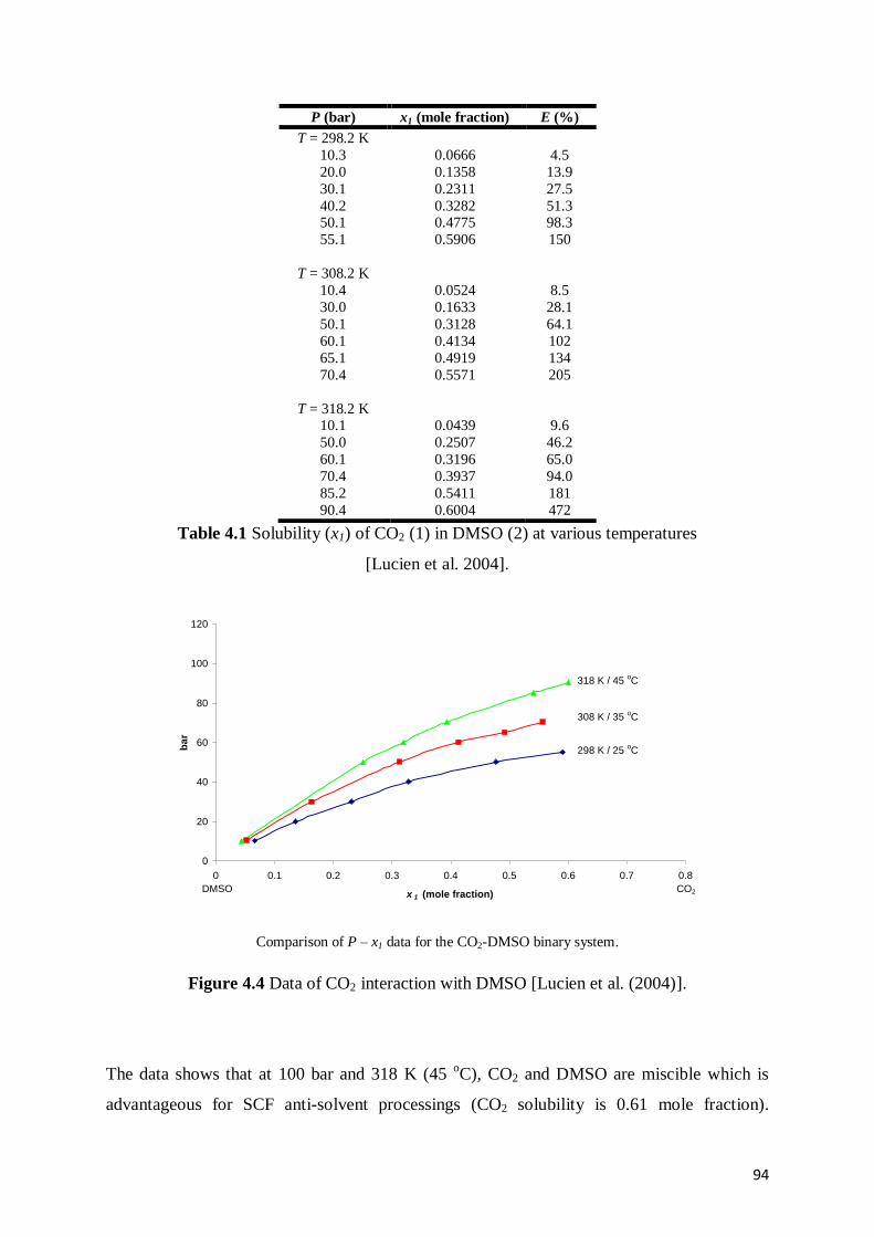
94
P (bar) x1 (mole fraction) E (%)
T = 298.2 K
10.3 0.0666 4.5
20.0 0.1358 13.9
30.1
40.2 50.1
55.1
T = 308.2 K
10.4
30.0
50.1
60.1
65.1
70.4
T = 318.2 K 10.1
50.0
60.1
70.4
85.2
90.4
0.2311
0.3282 0.4775
0.5906
0.0524
0.1633
0.3128
0.4134
0.4919
0.5571
0.0439
0.2507
0.3196
0.3937
0.5411
0.6004
27.5
51.3 98.3
150
8.5
28.1
64.1
102
134
205
9.6
46.2
65.0
94.0
181
472
Table 4.1 Solubility (x1) of CO2 (1) in DMSO (2) at various temperatures
[Lucien et al. 2004].
0
20
40
60
80
100
120
0 0.1 0.2 0.3 0.4 0.5 0.6 0.7 0.8
x 1 (mole fraction)
ba
r
DMSO CO2
318 K / 45 oC
298 K / 25 oC
308 K / 35 oC
Comparison of P – x1 data for the CO2-DMSO binary system.
Figure 4.4 Data of CO2 interaction with DMSO [Lucien et al. (2004)].
The data shows that at 100 bar and 318 K (45 oC), CO2 and DMSO are miscible which is
advantageous for SCF anti-solvent processings (CO2 solubility is 0.61 mole fraction).
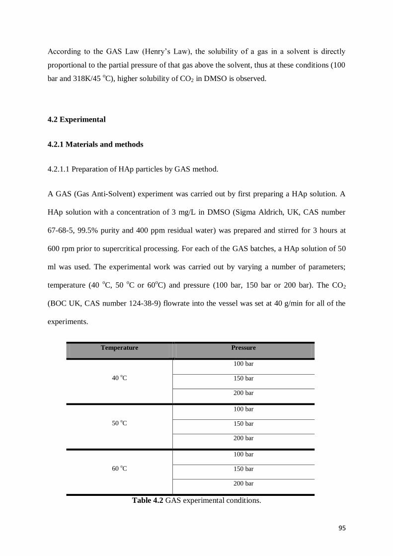
95
According to the GAS Law (Henry’s Law), the solubility of a gas in a solvent is directly
proportional to the partial pressure of that gas above the solvent, thus at these conditions (100
bar and 318K/45 oC), higher solubility of CO2 in DMSO is observed.
4.2 Experimental
4.2.1 Materials and methods
4.2.1.1 Preparation of HAp particles by GAS method.
A GAS (Gas Anti-Solvent) experiment was carried out by first preparing a HAp solution. A
HAp solution with a concentration of 3 mg/L in DMSO (Sigma Aldrich, UK, CAS number
67-68-5, 99.5% purity and 400 ppm residual water) was prepared and stirred for 3 hours at
600 rpm prior to supercritical processing. For each of the GAS batches, a HAp solution of 50
ml was used. The experimental work was carried out by varying a number of parameters;
temperature (40 oC, 50
oC or 60
oC) and pressure (100 bar, 150 bar or 200 bar). The CO2
(BOC UK, CAS number 124-38-9) flowrate into the vessel was set at 40 g/min for all of the
experiments.
Temperature Pressure
40 oC
100 bar
150 bar
200 bar
50 oC
100 bar
150 bar
200 bar
60 oC
100 bar
150 bar
200 bar
Table 4.2 GAS experimental conditions.

96
The GAS processing rig consisted of a 500 ml pressure vessel (Parr, Moline, USA) in which
a beaker containing the HAp solution was placed. The CO2 flowrate was set by the CO2
pump, using integral software (Thar Instrument Process Suite, version 2.05). Prior to GAS
processing, the rig was heated to the desired operating temperature (to within ± 1 oC), also by
the integral software. CO2 was then introduced into the system to reach the respective set
pressure. A back pressure regulator was used to maintain the pressure within the system (to
within ± 1 bar). After 6 hours the CO2 supply was stopped and the supercritical processing rig
was depressurised and cooled down. During the process, the CO2 had stripped the DMSO
which led to supersaturation and the formation of HAp particles. The particles produced were
retained inside the beaker and were removed for analysis. The waste DMSO solvent was
collected by opening the cyclone valve and was disposed in a safe manner. Before disposal,
the DMSO was analysed for any HAp content. Each GAS experimental condition was
repeated 6 times. The results were reproducible and the experimental data is presented in
Appendix 4B.
4.2.1.2 Preparation of HAp particles by SEDS method.
HAp powder used in the SEDS processing was prepared via the wet chemistry method as
mentioned in Chapter 3. The HAp solution was prepared by dissolving 3 mg of HAp in a litre
of dimethyl sulfoxide (DMSO), (Sigma Aldrich, UK, CAS number 67-68-5) acted as the
solvent. The solution was stirred at 600 rpm for 3 hours prior to supercritical processing. For
each SEDS experiment, a HAp solution of 500 ml was used. The experimental work was
carried out by varying a number of parameters: solvent flowrate (1 ml/min and 2 ml/min),
CO2 flowrate (20 g/min, 40 g/min and 60 g/min) and temperature (40 oC and 50
oC), as
shown in Table 4.3. The operating pressure was set at 150 bar for all of the experimental
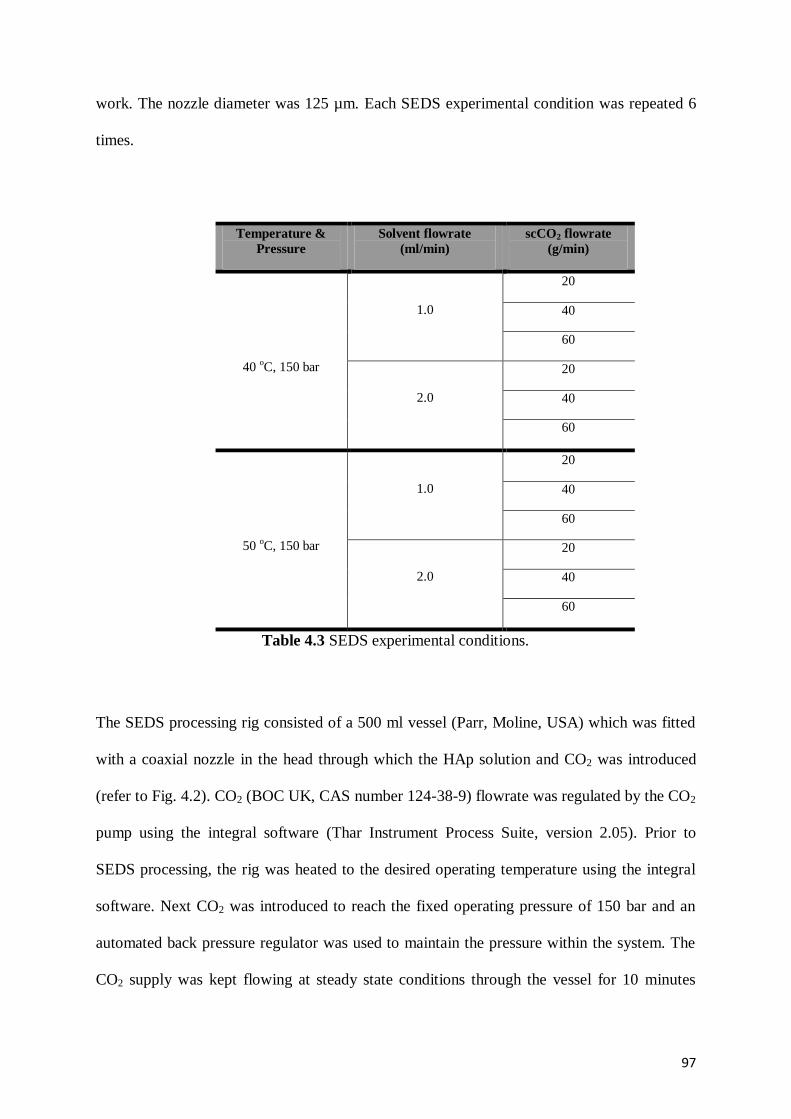
97
work. The nozzle diameter was 125 µm. Each SEDS experimental condition was repeated 6
times.
Temperature &
Pressure
Solvent flowrate
(ml/min)
scCO2 flowrate
(g/min)
40 oC, 150 bar
1.0
20
40
60
2.0
20
40
60
50 oC, 150 bar
1.0
20
40
60
2.0
20
40
60
Table 4.3 SEDS experimental conditions.
The SEDS processing rig consisted of a 500 ml vessel (Parr, Moline, USA) which was fitted
with a coaxial nozzle in the head through which the HAp solution and CO2 was introduced
(refer to Fig. 4.2). CO2 (BOC UK, CAS number 124-38-9) flowrate was regulated by the CO2
pump using the integral software (Thar Instrument Process Suite, version 2.05). Prior to
SEDS processing, the rig was heated to the desired operating temperature using the integral
software. Next CO2 was introduced to reach the fixed operating pressure of 150 bar and an
automated back pressure regulator was used to maintain the pressure within the system. The
CO2 supply was kept flowing at steady state conditions through the vessel for 10 minutes

98
(ensuring constant and stable pressure within the system) before the HAp solution was
introduced into the supercritical vessel. When the HAp solution was finished, CO2 was kept
flowing for 30 minutes in order to purge any residual solvent that might remain in the vessel.
The CO2 supply was then stopped and the supercritical processing rig was depressurised and
cooled down. The particles produced were collected at the bottom of the vessel on a steel
mesh filter. The waste DMSO solvent was collected by opening the cyclone valve and was
disposed in a safe manner. Before disposal, the DMSO was analysed for any HAp content.
4.3 Particle characterisation techniques
The particle characterisation techniques are the same as mentioned in Chapter 3, section 3.3.
99
4.4 Results and discussion
This study was carried out to evaluate the potential of supercritical fluid (SCF) processing,
specifically by the GAS Anti-Solvent (GAS) and Solution Enhanced Dispersion by
Supercritical Fluids (SEDS) methods in producing nanoparticles of hydroxyapatite (HAp).
This work is the first report in the production of HAp by SCF methods. The only other work
that utilises SCF and HAp is the work of Barry [Barry et al. (2008)] who published an in vitro
study of hydroxyapatite based photocurable polymer composites prepared by laser
stereolithography and SCF extraction. The work in this thesis was carried out in order to
compare HAp particles produced from the sol-gel (wet chemistry) technique and SCF
methods and assessing any advantages and disadvantages among these two procedures. In
addition, the potential of using the SCF technique to produce a non-viral gene vector was also
evaluated. SEDS method has been shown to achieve better mixing through turbulent flow
which can lead to a change in particle size when compared to those produced by GAS
[Palakodaty et al. (1998)]. The particles produced from the GAS method were compared to
those from the SEDS method. The characterisations undertaken were to determine the
functional groups (FTIR), phase analysis (XRD), morphology (SEM) and the particle size
estimations (TEM & HPPS) of the as prepared SCF processed HAp.
The FTIR analysis showed the occurrence of absorption peaks for HAp for both SCF
methods, which consisted of peaks representing the phosphate groups (PO43-
) and hydroxide
groups (OH-) for all the particle samples obtained. The FTIR spectra of some of the particle
samples obtained from both methods are combined in Figure 4.5 below:

100
0
0.5
1
1.5
2
2.5
400 600 800 1000 1200 1400 1600 1800 2000 2200 2400 2600 2800 3000
Wavelength (cm-1
)
Arb
itra
ry
P - O
O - H
C - O
GAS, 40 oC, 150 bar
GAS, 50 oC, 150 bar
SEDS, 40 oC, 1ml/min, 60 g CO2/min
SEDS, 40 oC, 2 ml/min, 60 g CO2/min
SEDS, 50 oC, 1 ml/min, 60 g CO2/min
SEDS, 50 oC, 2 ml/min, 60 g CO2/min
C - O
Figure 4.5 FTIR spectra of some GAS & SEDS processed HAp samples.
FTIR results indicated the presence of HAp by the bands for the P-O stretching vibration at
565 – 601 cm-1
and 960 – 965 cm-1
which corresponded to the phosphate (PO43-
) ions
[Kawata et al. (2004) & Miyaji et al. (2005)]. The peaks assigned to the stretching modes of
hydroxyl groups (OH-) in hydroxyapatite were at 632 cm
-1 and 3571 cm
-1 [Miyaji et al.
(2005), Varma & Babu (2005)]. The HAp formed by both approaches in this study is still
shown to be of type B substitution (whereby carbonate ions, CO32-
have substituted some of
the PO43-
ions in the apatitic structure) by the C-O peaks observed at 1418 cm-1
and 1462 cm-1
[Varma & Babu (2005)] as previously observed by the wet chemistry technique (refer to Fig.
4.5). The presence of type B carbonate in the apatite lattice has been shown to cause an
increase in its solubility both in vitro and in vivo tests [Krajewski et al. (2005)].

101
In terms of the XRD analysis, the formation of hydroxyapatite is indicated by the
characteristic peak occurred at 2θ = 31.8o as shown on Figure 4.6 [Shimbayashi et al. (1996)].
The narrow peaks on the XRD spectra indicated a high degree of crystallinity (averages of 68
%) of the hydroxyapatite crystals formed.
0
500
1000
1500
2000
2500
3000
3500
4000
4500
5000
20 25 30 35 40 45 50 55 60 65 70 75 80
2θ (o)
Arb
itra
ry GAS 40 oC, 100 bar
HAp
GAS 50 oC, 150 bar
SEDS 40 oC, 1, 60
SEDS 40 oC, 2, 60
SEDS 50 oC, 1, 60
SEDS 50 oC, 2, 60
Figure 4.6 XRD patterns of some GAS & SEDS HAp samples.
In the DLS analyses, the HAp produced by the GAS technique, showed that the particle size
decreased slightly at a lower temperature and also at higher pressure. As an example, for
HAp produced by GAS technique at operating temperature of 50 oC and a pressure of 100
bar, particles with an average size of 177 nm were obtained. Meanwhile, at an operating
temperature of 50 oC and pressure of 150 bar, particles with an average size of 173 nm were
produced. Particles produced at 60 oC had an average size of 186 nm. This can be explained
by the interactions between the scCO2 and DMSO at specific temperatures and pressures. At
lower operating temperatures for a given pressure, there is a higher solubility of CO2 in

102
DMSO and expansion of DMSO will occur as reported by Lucien [Lucien et al. (2004)]. This
is due to the increase in the density of CO2 and the corresponding increase in the solubility of
CO2 in the liquid phase. Higher amount of CO2 leads to smaller particles induced by higher
supersaturation. The DLS data for the GAS technique is shown in Table 4.4.
GAS sample
(Temperature oC,
pressure, bar)
Particle size by
DLS, filtered
(nm)
40, 150 168 ± 5
50, 150 173 ± 3
60, 150 186 ± 4
50, 100 177 ± 5
50, 200 163 ± 6
Table 4.4 Particle sizing for HAp produced by GAS technique.
For the SEDS samples, the particle size decreased with temperature and antisolvent to solvent
ratio. In respect of operating temperature, at a given solvent flowrate (1 ml/min) and
antisolvent flowrate (60 g/min), the HAp particles produced at 40 oC have average particle
sizes of 131 nm. For the same given solvent and antisolvent flowrate but at temperature of 50
oC, the average particle size is 141 nm. In term of antisolvent to solvent ratio, the particle size
decreased with higher ratio of antisolvent to solvent. The HAp sample produced at operating
conditions of temperature at 40 oC, with 1 ml/min of solvent flowrate and 60 g/min of
antisolvent (antisolvent to solvent ratio of 60) gave particle size of 131 nm. In contrast, the
HAp sample produced at operating conditions of temperature at 40 oC, with 2 ml/min of
solvent flowrate and 60 g/min of antisolvent (antisolvent to solvent ratio of 30) gave particle
size of 153 nm. This could be explained by the better mixing of the scCO2 with the solvent,
thus increasing the solvent extraction. More CO2 anti-solvent within the system, leads to

103
faster supersaturation that forms smaller nuclei. The DLS data for the SEDS technique is
shown in Table 4.5.
SEDS sample
(Temperature, solvent
flowrate, CO2 flowrate)
CO2 / solvent ratio
flowrate
Particle size by
DLS filtered
(nm)
40, 1, 20 20 152 ± 3
40, 1, 40 40 144 ± 3
40, 1, 60 60 131 ± 4
40, 2, 20 10 167 ± 6
40, 2, 40 20 154 ± 5
40, 2, 60 30 153 ± 4
50, 1, 20 20 166 ± 5
50, 1, 40 40 149 ± 4
50, 1, 60 60 141 ± 5
50, 2, 20 10 185 ± 3
50, 2, 40 20 164 ± 4
50, 2, 60 30 159 ± 3
Table 4.5 Particle sizing for HAp produced by SEDS technique.
The DLS data showed that the particle size produced by the SEDS technique gave smaller
particle size as compared to the GAS technique. As an example, the SEDS processed HAp at
40 oC and scCO2 for a solvent ratio flowrate of 60 produced an average particle size of 131
nm, whereas the GAS technique at 40 oC, 150 bar and scCO2 of 40 g/min, gave an average
particle size of 168 nm. This would be due to the faster and better mixing of antisolvent to
solvent in the SEDS technique as compared to the GAS technique which is slower.
SEM images reveal the morphology of the produced particles, which exhibit a circular
appearance. The images show that the particles consist of smaller units which agglomerate
into larger units when contacted with each other. Some of the SEM images for the GAS and
SEDS processed HAp are shown in Figure 4.7.

104
a) GAS at 40 oC and 150 bar
b) GAS at 50 oC and 150 bar
c) SEDS at 40 oC, 1 ml/min,
60 gCO2/min
d) SEDS at 50 oC, 1 ml/min,
60 gCO2/min
e) SEDS at 40 oC, 2 ml/min,
60 gCO2/min
f) SEDS at 50 oC, 2 ml/min,
60 gCO2/min
Figure 4.7 SEM images of some of the GAS and SEDS samples.

105
TEM is a very useful tool in estimating the particle size of nanomaterials [Ma & Liu
(2009)]. From the SEDS processing, it was shown that the particle size decreased with
higher ratio of CO2 flowrate with the solvent flowrate. This regime facilitates rapid
supersaturation, extracting the solvent more efficiently which leads to nucleation and
subsequent production of particles [Palakodaty et. al. (1998)]. Other workers have
reported that the dispersion in the jet at the nozzle outlet facilitates rapid (< 1 second)
formation of particles of small size [Hanna (1994)]. This study also showed that HAp can
be recrystallised by GAS and SEDS processing with particles size decreased in respect of
the processing conditions of temperature, pressure and scCO2 to solvent flowrate.

106
Figure 4.8 TEM images of some of the GAS and SEDS samples.
(a) GAS at 40 oC and 150 bar (b) GAS at 60
oC and 150 bar
DLS: 168 ± 5 nm
DLS: 186 ± 4 nm
(c) GAS at 50 oC and 100 bar (d) GAS at 50
oC and 200 bar
DLS: 177 ± 5 nm
DLS: 163 ± 6 nm
(e) SEDS at 40 oC, 1 ml/min and
60 g/min of CO2
(f) SEDS at 40 oC, 2 ml/min and
60 g/min of CO2
DLS: 131 ± 4 nm
DLS:153 ± 4 nm
(g) SEDS at 50 oC, 1 ml/min and
60 g/min of CO2
(h) SEDS at 50 oC, 2 ml/min and
60 g/min of CO2
DLS:141 ± 5 nm
DLS:159 ± 3 nm
107
4.5 Conclusions
In this study, HAp particles were recrystallised by the GAS and SEDS supercritical
processing techniques. The HAp samples produced by both techniques gave similar
characterisations in term of FTIR, XRD and SEM analyses. They only differ in the
particle size. The particle size decreased with respect to the operating conditions of
temperature, pressure and antisolvent to solvent ratio. Overall, SEDS technique yield
smaller particle size as compared to GAS technique.

108
4.6 References:
Adschiri, T. Arai, K. 2002. Hydrothermal synthesis of metal oxide nanoparticles
under supercritical conditions, In: Ya-Ping Sun (Ed.), Supercritical Fluid Technology
in Material Science and Engineering, Marcel Dekker Inc., New York, pp. 311 - 325.
Barry, J .J. A. Evseev, A. V. Markov, M. A. Upton, C. E. Scotchford, C. A. Popov, V.
K. Howdle, S. M. 2008. In vitro study of hydroxyapatite-based photocurable polymer
composites prepared by laser stereolithography and supercritical fluid extraction, Acta
Biomaterialia 4, Issue 6: 1603 – 1610.
Byrappa, K. Ohara, S. Adschiri, T. 2008. Nanoparticles synthesis using supercritical
fluid technology – towards biomedical applications, Advanced Drug Delivery Review
60: 299 – 327.
Chattopadhyay, P. Gupta, R. B. 2002. Supercritical CO2 based production of
magnetically responsive micro- and nanoparticles for drug targeting, Ind. Eng. Chem.
Res. 41: 6049 – 6058.
DeSimone, J. M. 2002. Practical approaches to green solvents, Science 297: 799 –
803.
Epple, M. Sokolova, V. 2008. Inorganic Nanoparticles as Carriers of Nucleic Acids
into Cells, Angew. Chem. Int. Ed. 47: 1382 – 1395.
Gallagher, P. M. Coffey, M. P. Krukonis, V. J. Klasutis, N. 1989. In Supercritical
Fluid science and Technology. Johnston, K. P. Penniger, J. M. L. Eds. ACS
Symposium Series 406, American Chemical Society, Washington DC.
Gallagher, P. M. Coffey, M. P. Krukonis, V. J. 1992. Gas Anti-Solvent
Recrystallisation of a Difficult to Comminute Explosive. J. of Supercritical Fluids 5:
130 – 142.
Goodarzi, M. Duchowicz, P. R. Freitas, M. P. Fernandez, F. M. 2010. Prediction of
the Hildebrand parameter of various solvents using linear and nonlinear approaches.
Fluid Phase Equilibria 293: 130 – 136.
Hanna, M. York, P. 1994. Patent WO 95/0122 1.
Hay, J. N. Khan, A. 2002. Environmentally friendly coatings using carbon dioxide as
the carrier medium, J. Mater. Sci. 37: 4743 – 4752.
Jenkins, R. Synder, R. L. 1996. Introduction to X-ray Powder Diffractometry, John
Wiley and Sons, New York.
Kawata, M. Uchida, H. Itatani, K. Okada, I. Koda, S. Aizawa, M. 2004. Development
of porous ceramics with well-controlled porosites and pore sizes from apatite fibers
and their evaluations, J. Mater. Sci. Mater. Med. 817 – 823.

109
Kenneth, T. D. Artie, M. 2003. Dimethylsulfoxide (DMSO) solvent formulation for
exterior aircraft coatings removal. 2003 Aerospace Coatings Removal and Coatings
Conference. 1 – 10.
Krajewski, A. Mazzocchi, M. Buldini, P. L. Ravaglioli, A. Tinti, Taddei, P. Fagnano,
C. 2005. Synthesis of carbonated hydroxyapatites: efficiency of the substitution and
critical evaluation of analytical methods, Journal of Molecular Structure. 744: 221 –
228.
Lucien, F. P. Rajasingam, R. Lioe, L. Tuan Pham, Q. 2004. Solubility of carbon
dioxide in dimethylsulfoxide and N-methyl-2-pyrrolidone at elevated pressure.
Journal of Supercritical Fluids 31: 227 – 234.
Ma, G. Liu, X. Y. 2009. Hydroxyapatite: Hexagonal or Monoclinic?, Crystal Growth
& Design Vol. 9, No. 7: 2991 – 2994.
Mishima, K. 2008. Biodegradable particle formation for drug and gene delivery using
supercritical fluid and dense gas, Advanced Drug Delivery Reviews 60: 411 – 432.
Miyaji, F. Kono, Y. Suyama, Y. 2005. Formation and structure of zinc-substituted
calcium hydroxyapatite, Mater. Res. Bull. 40: 209 – 213.
Palakodaty, S. York, P. Pritchard, J. 1998. Supercritical fluid processing of materials
from aquoes solutions: the application of SEDS to lactose as a model substance,
Pharm. Res. 15: 1835 – 1843.
Palakodaty, S. Sloan, R. Kordikowski, A. 2002. Pharmaceutical and biological
materials processing with supercritical fluids, In: Ya-Ping Sun (Ed.), Supercritical
Fluid Technology in Material Science and Engineering, Marcel Dekker Inc., New
York, pp. 439 – 490.
Pons, M. N. Vivier, H. Delcour, V. Authelin, J. R. Pailleres-Hubert, L. 2002.
Morphological analysis of pharmaceutical powders, Powder Tech. 128: 276 – 286.
Shimbayashi, S. Hashimoto, N. Kawamura, H. Uno, T. 1996. Mineral Scale
Formation and Inhibition, In: Amjad, Z (Ed.), Plenum Press: New York, 14 – 15.
Tservistas, M. Levy, M. S. Lo-Yim, M. Y .A. O’Kennedy, R .D. York, P. Humphrey,
G. O. Hoare, M. 2001. The formation of Plasmid DNA loaded Pharmaceutical
Powders Using Supercritical Fluid Technology, John Wiley & Sons, Inc.
Varma, H. Babu, S. S. 2005. Synthesis of calcium phosphate bioceramics by citrate
gel pyrolysis method, Ceram. Int. 31: 109 – 114.

110
5.0 A systematic investigation of Calcium Phosphates (CaP) precipitation
processes
5.1 Introduction
A systematic study on the formation of calcium phosphates by varying the calcium to
phosphorus ratio is reported in this chapter. The calcium precursor used is calcium
nitrate tetrahydrate, Ca(NO3)2.4H2O, the same calcium precursor as used in the sol-gel
method and supercritical fluid (SCF) work mentioned in Chapter 3 and 4. Meanwhile,
the phosphate precursor is diammonium phosphate, (NH4)2HPO4, substituting
phosphorus pentoxide (P2O5) as the phosphate precursor. This new calcium phosphate
investigation was carried out by two methods, the wet chemistry (direct precipitation)
and supercritical anti-solvent (SEDS) methods.
5.2 Materials and methods
5.2.1 Materials
Calcium nitrate tetrahydrate, Ca(NO3)2.4H2O [CAS number 13477-34-4],
diammonium phosphate (NH4)2HPO4 [CAS number 7783-28-0], concentrated
aqueous ammonia (NH4OH) [CAS number 7664-41-7] and dimethyl sulfoxide,
DMSO [CAS number 67-68-5, 99.5% purity and 400 ppm residual water)] were
obtained from Sigma-Aldrich UK and were used without further purification. The
CO2 for SEDS processing [CAS number 124-38-9] was supplied by BOC UK (99%
purity).

111
5.2.2 Direct precipitation method
The direct precipitation method was carried out according to the procedure reported
by Jarcho et al. (1979). The molar ratio studies conducted for the Ca/P were
1.00:2.50, 1.50:2.00, 1.50:1.50, 2.00:1.50, 1.67:1.00 and 2.50:1.00. This study was
based upon the main Ca/P ionic ratios mentioned on Table 2.1. As an example, for the
Ca/P molar ratio of 1.50:1.50, 150 mM each of calcium nitrate tetrahydrate and
diammonium phosphate precursors were dissolved in 100 ml of double distilled water.
The pH of both solutions was corrected between 11 and 12 by adding concentrated
aqueous ammonia (35% concentration). The calcium nitrate solution was vigorously
stirred at 1200 rpm at a temperature of 20 oC and then the diammonium phosphate
solution was added dropwise for a duration of 30 minutes (dropwise flowrate of 3.33
ml/min). The reaction mixture was stirred for 12 hours and then centrifuged at 2000
rpm for 10 minutes, the supernatant decanted and the precipitate was resuspended in
double distilled water. This washing procedure was repeated a further two times. The
centrifuged precipitate was then dried at 80 oC for 24 hours and ground with a pestle
and mortar.

112
5.2.3 SEDS method
The SEDS method was carried out according to the procedure described earlier in
Chapter 3. The molar ratios studied for this method were based upon the flowrate of
the calcium and phosphate precursors dissolved in DMSO into the reaction vessel, via
two separate nozzles. An additional peristaltic pump (Thar Tech. Inc.) was used to
deliver the calcium precursor solution into the reaction vessel. The flowrates studied
were 1) 0.50 ml/min of calcium precursor : 1.50 ml/min of phosphate precursor
(molar ratio of 0.33), 2) 1.00 ml/min of calcium precursor : 1.00 ml/min of phosphate
precursor (molar ratio of 1.00) and 3) 1.50 ml/min of calcium precursor : 0.50 ml/min
of phosphate precursor (molar ratio of 3.00) at fixed concentrations of 100 mM for
both precursors. This study was based upon the main Ca/P ionic ratios mentioned on
Table 2.1, but fewer Ca/P molar ratios were studied compared to the direct
precipitation method due to the limitation of the peristaltic pump used for introducing
the calcium precursor solution into the reaction vessel. The SEDS processing
conditions were set at 50 oC and 150 bar for all of the experimental work. These
conditions were chosen as CO2 has high solubility (0.30 mole fraction) and volume
expansion (50%) in DMSO. The CO2 supply into the reaction vessel was maintained
at 60 g/min which provided a high antisolvent to solvent ratio within the system.
These conditions produced smaller HAp particles as observed in Chapter 4. Each
molar ratio processed by SEDS was repeated 6 times. The results were reproducible
and the experimental data is presented in Appendix for Chapter 5.

113
5.2.4 Particle characterisation techniques
Particle characterisation techniques undertaken were similar to those mentioned in
Chapter 3 and 4, namely X-ray Diffraction (XRD) for phase analysis, FTIR analysis
for determining the functional groups, Dynamic Light Scattering (DLS) and
Transmission Electron Microscope (TEM) and Scanning Electron Microscope (SEM)
for particle size estimation and particle morphology.
5.3 Results and discussion
5.3.1 Effect of molar ratios on the precipitates collected
5.3.1.1 Direct precipitation method
The molar ratio studies conducted for the direct precipitation method were at the Ca/P
ratios as shown in Table 5.1 below:
Ca/P precursor concentration
(mM/mM)
Ca/P ratio
100/250 0.40
150/200 0.75
150/150 1.00
200/150 1.33
167/100 1.67
250/100 2.50
Table 5.1 Ca/P molar ratio studied for the direct precipitation method.

114
The XRD patterns for Ca/P ratios 2.50, 1.67 and 1.33 showed the occurrence of
dicalcium phosphate dihydrate (DCPD) phase, otherwise known as brushite, due to
the most intense peak occurring at 20.9o
2θ and other corresponding peaks at 29.2o,
30.5o, 31.3
o, 34.2
o, 34.4
o, 37.1
o, 41.6
o, 42.0
o, 43.4
o, 50.2
o, and 59.5
o. The XRD
patterns for Ca/P ratios of 2.50, 1.67 and 1.33 are shown in Figure 5.1 below:
0
1000
2000
3000
4000
5000
6000
7000
8000
9000
20 25 30 35 40 45 50 55 60 65 70 75 80
2 theta (o)
Arb
itra
ry
Dicalcium phosphate dihydrate (DCPD)
Ca/P ratio = 1.33
Ca/P ratio = 1.67
Ca/P ratio = 2.50
Figure 5.1 XRD patterns of the precipitates for the Ca/P ratios of
2.50, 1.67 and 1.33.

115
The XRD patterns for the Ca/P ratios of 1.00, 0.75 and 0.40 are shown in Figure 5.2.
The Ca/P ratios of 1.00 and 0.75 also showed the occurrence of the dicalcium
phosphate dihydrate (DCPD)/brushite phase. For the Ca/P ratio of 0.40, the phase
determination from its XRD peaks is unclear. This maybe due to the low
concentrations of both precursors used, which induces incomplete reaction as a result
of a low pH (5.58) within the formation process.
0
1000
2000
3000
4000
5000
6000
7000
8000
9000
20 25 30 35 40 45 50 55 60 65 70 75 80
2 theta (o)
Arb
itra
ry
Dicalcium phosphate dihydrate (DCPD)
Ca/P ratio = 1.00
Ca/P ratio = 0.75
Ca/P ratio = 0.40
Figure 5.2 XRD patterns of the precipitates for the Ca/P ratios of
1.00, 0.75 and 0.40.
The FTIR spectra revealed that for the Ca/P ratios of 2.50, 1.67, 1.33, 1.00 and 0.75
have similar absorbance patterns, due to their phase identified as brushite from the
XRD analysis. The bands at 526 and 577 cm-1
correspond to the medium intensity for
P-O bending. Meanwhile, the bands at 660 and 790 correspond to the medium
intensity for OH out of plane bending. Strong intensities for P-O (H) stretching are
observed for the 875 and 985 bands. The 1060 and 1135 bands correspond to the

116
strong intensity for PO stretching. The 1217 band corresponds to strong intensity for
motion of hydroxyl group and lastly, the 1652 band corresponds to strong intensity for
inplane bending of water molecule [Petrov et al. (1967), Kawata et al. (2004) and
Mijaya et al. (2005)]. For the Ca/P ratio of 0.40, the peaks assigned to the phosphate
group are observed to be much broader, indicating the excess phosphate ions in the
precipitates as compared to other Ca/P ratios. The FTIR spectra for the Ca/P ratios of
2.50, 1.67, 1.33, 1.00, 0.75 and 0.40 are shown in Figure 5.3.
0
0.5
1
1.5
2
2.5
400 600 800 1000 1200 1400 1600 1800 2000
Wavenumber (cm-1
)
Arb
itra
ry
Ca/P ratio = 2.50
Ca/P ratio = 1.67
Ca/P ratio = 1.33
Ca/P ratio = 1.00
Ca/P ratio = 0.75
Ca/P ratio = 0.40
P-O P-OO-H O-HO-H
Figure 5.3 FTIR spectra for the precipitates from the direct precipitation
method for Ca/P ratios of 2.50, 1.67, 1.33, 1.00, 0.75 and 0.40.

117
5.3.1.2 SEDS method
The Ca/P precursor flowrates investigated in the SEDS experiments are shown in
Table 5.2 below:
Ca/P precursor flowrate
(ml/ml per min, at fixed 100mM
concentration for each precursor)
Ca/P ratio
1.50/0.50 3.00
1.00/1.00 1.00
0.50/1.50 0.33
Table 5.2 Ca/P molar ratios studied for the SEDS method.
Fewer Ca/P molar ratios were studied compared to the direct precipitation method due
to the limitation of the peristaltic pump used for introducing the calcium precursor
solution into the reaction vessel. The XRD patterns for the Ca/P ratios of 3.00 and
1.00 showed the occurrence of dicalcium phosphate anhydrous (DCPA) phase,
otherwise known as monetite by the most intense peak occurring at 30.3o 2θ and other
corresponding peaks at 26.5o, 32.5
o, 33.0
o, 35.9
o, 47.5
o, 49.3
o and 53.1
o. The phase
for the Ca/P ratio of 0.33 might be monocalcium phosphate anhydrous, MCPA which
has intense peaks at 26.6o, 29.4
o, 30.2
o and 39.0
o. The XRD patterns for the Ca/P
ratios of 3.00, 1.00 and 0.33 are shown in Figure 5.4.

118
0
1000
2000
3000
4000
20 25 30 35 40 45 50 55 60 65 70 75 80
2 theta (o)
Arb
itra
ry
Dicalcium phosphate anhydrous (DCPA)
Ca/P ratio = 3.00
Ca/P ratio = 1.00
Ca/P ratio = 0.33
Figure 5.4 XRD patterns of the precipitates from the SEDS method for Ca/P
ratios of 3.00, 1.00 and 0.33.
The FTIR spectra for the Ca/P ratios of 3.00 and 1.00 showed the presence of medium
intensity for P-O bending for 526 cm-1
band. The 750 and 825 cm-1
band correspond
to medium intensity for OH out of plane bending. Meanwhile, the 960 cm-1
band
corresponds to strong intensity for P-O (H) stretching and the 1008 and 1060 cm-1
band correspond for strong intensities for PO stretching. The presence of carbonate
(CO32-
) was identified by the broad peak at 1418 - 1462 cm-1
, which is not seen in the
FTIR spectra of the direct precipitation method (see Figure 5.3). Lastly, the 1652 cm-1
band correspond to strong intensity for inplane bending of water molecule [Petrov et
al. (1967), Kawata et al. (2004) and Mijaya et al. (2005)]. The FTIR spectra for the
Ca/P ratios of 3.00, 1.00, and 0.33 are shown in Figure 5.5.

119
0
0.2
0.4
0.6
0.8
1
1.2
1.4
1.6
400 600 800 1000 1200 1400 1600 1800 2000
Wavenumber (cm-1
)
Arb
itra
ry
Ca/P ratio = 0.33
Ca/P ratio = 1.00
Ca/P ratio = 3.00
P-O O-H P-O C-O O-H
Figure 5.5 FTIR spectra for the precipitates produced by the SEDS method
for Ca/P ratios of 3.00, 1.00 and 0.33.
5.3.1.3 Ca/P phase formation
Precipitation of solids from a homogeneous solution involves generation of
supersaturation followed by nucleation and crystal growth. Aqueous calcium
phosphate solution comprises of many different ions. The composition of these ions
depends on the solution pH. The generation of supersaturation is highly dependent on
the calcium and phosphorus concentration, the pH and temperature, and in the case of
the SEDS method, pressure.
Brushite (dicalcium phosphate dehydrate, DCPD) was the only precipitated phase in
the majority of the direct precipitation experiments, except for the experiment with a
Ca/P ratio of 0.40, which did not show the intense peaks corresponding to the brushite

120
phase. This is in agreement with the identification of brushite phase from the literature
[Boistelle and Lopez-Velero (1990), Elliot (1994), Madsen and Christaensson (1991),
Ferreira et al. (20053), Marshall and Nancollas (1969), Abbona et al. (1998) and Wu
and Nancollas (1998)]. The formation of brushite at a pH lower than 6.5 has been
reported by numerous investigators [Boistelle and Lopez-Velero (1990), Elliot (1994),
Madsen and Christaensson (1991), Faffeira et al. (2005), Marshall and Nancollas
(1969), Abbona et al. (1998)]. Boistelle and Lopez-Valero (1990) and Abbona et al.
(1998) reported that below pH 6.5, brushite is the dominant phase, whereas, above pH
6.5, formation of amorphous calcium phosphate (ACP) and octacalcium phosphate
(OCP) is more likely. On the other hand, Wu and Nancollas (1998) claimed that
although brushite and octacalcium phosphate readily precipitate from solution, they
are thermodynamically metastable with respect to hydroxyapatite, HAp, and serve as
a precursor phase. It has been reported that the kinetic coefficients of OCP and HAp
are smaller than that of DCPD by 10 and 18 orders of magnitude at pH 6.5 [Boistelle
& Lopez-Velero (1990)]. Even though the initial pH of the calcium and phosphorus
precursor solution were brought between 11 and 12, the pH decreased during the
precipitation process due to the presence of water in the solutions (200 ml of distilled
water was used for each precipitation sample) and the slow absorption of carbon
dioxide (CO2) from the environment. This in turn would have lead to the formation of
carbonic acid within the reaction solution, which made the solution acidic (pH 6.0).
Furthermore, as the concentration of calcium and phosphorus was increased in the
reaction vessel (beaker), the nucleation occurred at a lower pH. Even for the same
calcium concentration, the nucleation pH was lower for a higher phosphate
concentration. The following equilibrium takes place during the precipitation process:

121
H2PO4-H
+ = HPO4
2- + 2H
+,
Ca2+
+ H2PO4- = CaH2PO4
+,
Ca2+
+ HPO42-
= CaHPO4.
The consumption of phosphate ion in the formation and growth of brushite would
decrease the pH of the solution because of the release of the hydrogen ions from
H2PO42-
dissociation. The higher the initial reagent concentration, the higher was the
concentration of the remaining acid and the lower was the nucleation pH
[Christoffersen et al. (1990), Boistelle & Lopez-Velero (1990), Hlabse & Walton
(1965)] (the pH values range was between 5.58 and 6.55 for the direct precipitation
for CaP ratios of 0.40 to 2.50).
The formation of brushite (direct precipitation method) and monetite (SEDS method)
phases are observed in the present condition of the study. The order of their
precipitation from a supersaturated solution is not only governed by the
thermodynamic solubility product, but also by kinetic factors. The precipitated phase
may undergo solution mediated transformation to more stable phases [Abbona et al.
(1986)].
At room temperature, the occurrence of mainly three crystalline phases has been
reported in the literature [Boistelle and Lopez-Velero (1990)]. In order of decreasing

122
solubility in water (H2O), they are brushite, octacalcium phosphate and
hydroxyapatite. In addition, amorphous calcium phosphate also precipites at room
temperature. Supersaturation needed for the formation of hydroxyapatite (HAp),
octacalcium phosphate (OCP) and brushite (DCPD) are in the order of HAp > OCP >
DCPD. Brushite nucleates more easily than OCP and HAp at low pH (in the pH range
of 5 to 6) [Boistelle and Lopez-Velero (1990)]. Therefore the formation and growth of
brushite is favoured in the present conditions of the study.
Meanwhile, for the SEDS method, monetite (dicalcium phosphate anhydrous, DCPA)
was the only precipitated phase observed for two of the CaP ratios, which are ratios of
3.00 and 1.00. Monetite is the anhydrous form of brushite (DCPD) and it is less
soluble than DCPD due to the absence of water inclusions. The formation of monetite
in these conditions was due to the lower pH as a result of a CO2 rich environment
within the system and also the use of DMSO instead of distilled water in dissolving
the precursors. The residual water in the DMSO is 400 ppm (Sigma Aldrich, UK,
CAS number 67-68-5, 99.5% purity), thus even with this small amount of water, the
formation of carbonic acid is possible inside a CO2 rich environment.

123
5.3.2 Effect of molar ratios on particle size and morphology
5.3.2.1 Direct precipitation method
A summary table containing the data for SEM, TEM and DLS for the direct
precipitation method is shown in Table 5.3. The brushite crystals produced had plate-
like morphology as observed by SEM. This morphology is in agreement with the
morphology observed by Arifuzzaman & Rohani (2004). TEM images for each of the
Ca/P ratios showed that the primary crystals are within the nanosized range
(approximately 50 – 80 nm). Since all of the wet precipitation samples are identified
as brushite, except for the Ca/P ratio of 0.40, they have similar characteristics in terms
of their morphologies and particle sizes. The particle size data showed that the mean
crystal sizes of the agglomerates are insensitive to the variation of initial calcium and
phosphorus concentration.
The particle sizes reported here are the filtered precipitation samples prior to the DLS
measurements. In the unfiltered samples, the particles rapidly aggregated to form
agglomerates while the filtered samples, the particles formed stable agglomerates. The
filtered samples resulted in smaller particles but the sizes still implied that aggregation
of the primary particles had occurred.

124
Table 5.3 SEM, TEM & DLS particle size data obtained from the direct precipitation
method.
Ca/P ratio SEM (scalebar = 20 μm) TEM DLS, filtered (nm)
0.40
216 ± 2
0.75
214 ± 3
1.00
215 ± 4
1.33
214 ± 2
1.67
218 ± 6
2.50
219 ± 7

125
5.3.2.2 SEDS method
A summarised table containing the data for SEM, TEM and DLS for the SEDS
method is shown in Table 5.4. The monetite crystals produced had grain-like
morphology as investigated by SEM (agglomerates with sizes approximately 50 µm).
The TEM images showed the fractured particles (particle sizes approximately
between 50 – 80 nm) from the larger particles shown in the SEM images.
Ca/P ratio
SEM (scalebar = 20
μm)
TEM
DLS, filtered
(nm)
0.33
218 ± 3
1.00
215 ± 6
3.00
217 ± 5
Table 5.4 SEM, TEM and DLS particle size data obtained from the SEDS method.

126
5.4 Conclusions
The particles produced by the direct precipitation method were identified to be mostly
the brushite phase. Meanwhile, the particles produced by the SEDS method were
observed to be the monetite phase. The pH of the reaction solution during the
precipitation process played an important role in forming these phases of CaP. It was
noted that the pH decreased during the direct precipitation process due to the presence
of carbonic acid by the mixture of water from the precursor solution and CO2 from the
environment, which made the reaction solution acidic. The decrease in the pH was
also due to the release of the hydrogen ions from the H2PO42-
dissociation. A further
investigation is to control the pH of the reaction solution throughout the precipitation
process.
It was the similar case for the SEDS method, where the CO2 rich environment within
the system has lowered the pH during the precipitation process due to the minute
amount of residual water in the DMSO (400 ppm) which may have turned it acidic
due to the formation of carbonic acid. DMSO was used to dissolve the precursors due
to its solubility with supercritical CO2 and produced monetite (DCPA), the anhydrous
form of brushite (DCPD).

127
5.5 References:
Abbona, F. Lundager-Madsen, H. E. Boistelle, R. 1986. The initial phases of calcium
and magnesium phosphates precipitated from solutions of high medium
concentrations, Journal of Crystal Growth, 74: 581 – 590.
Abbona, F. Christiansson, F. Angela, M. F. Lundager-Madsen, H. E. 1998. Crystal
habit and growth conditions of brushite, CaHPO4.2H2O, Journal of Crystal Growth,
131: 331 – 346.
Arifuzzaman, S. M. Rohani, S. 2004. Experimental study of brushite precipitation,
Journal of Crystal Growth, 267: 624 – 634.
Boistelle, R. Lopez-Velero, I. 1990. Growth units and nucleation: The case of calcium
phosphates, Journal of Crystal Growth, 102: 609 – 617.
Christoffersen, M. R. Christoffersen, J. Kibalczyc, W. 1990. Apparent solubilities of
two amorphous calcium phosphates and of octacalcium phosphate in the temperature
range 30 – 42 oC, Journal of Crystal Growth, 106: 349 – 354.
Elliot, J. C. 1994. Structure and Chemistry of the Apatites and Other Calcium
Orthophosphates, Elsevier, Amsterdam.
Ferreira, A. Oliveira, C. Rocha, F. 2003. The different phases in the precipitation of
dicalcium phosphate dihydrate, Journal of Crystal Growth, 252: 599 – 611.
Hlabse, T. Walton, A. G. 1965. The nucleation of calcium phosphate from solution,
Analytica Chimica Acta, 33: 373 – 377.
Jarcho, M. Salsbury, L. Thomas, M. B. Doremus, R. H. 1979. Synthesis and
fabrication of beta-tricalcium phosphate (whitlockite) ceramics for potential prosthetic
applications, Journal of Materials Science, 14: 142 – 150.
Kawata, M. Uchida, H. Itatani, K. Okada, I. Koda, S. M. Aizawa, M. 2004.
Development of porous ceramics with well-control porosites and pore sizes from
apatite fibers and their evaluations, Journal of Material Science. Med., 817 – 823.
Lundager-Madsen, H. E. Christaensson, F. 1991. precipitation of calcium phosphate
at 40 oC from neutral solution, Journal of Crystal Growth 114: 613 – 618.
Miyaji, F. Kono, Y. Suyama, Y. 2005. Formation and structure of zinc-substituted
calcium hydroxyapatite, Materials Reserach Bulletin 40: 209 – 213.
Marshall, R. W. Nancollas, G. H. 1969. The kinetics of crystal growth of dicalcium
phosphate dihydrate, Journal of Physical Chemistry, 73 (11): 3838 – 3833.
Petrov, I. Soptrajanov, B. Fuson, N. Lawson, J. R. 1967. Spectrochim Acta 23A:
2637.

128
Wu, W. Nancollas, G. H. 1998. The dissolution and growth of sparingly soluble
inorganic salts: A kinetic and surface energy approach, Pure Applied Chemistry, 70
(10): 1867 – 1872.

129
6.0 Attachment of calcium phosphate particles prepared by sol-gel, supercritical
anti-solvent and new calcium phosphate route with plasmid DNA (pDNA) and
in-vitro transfection studies of CaP-pDNA post co-precipitation complexes
6.1 Introduction
The technique of calcium phosphate co-precipitation with plasmid DNA (pDNA) for
in vitro transfection is used as a routine laboratory procedure [James et al. (1987)].
This method relies heavily on the fact that divalent metal cations, such as Ca2+
, Mg2+
,
Mn2+
, and Ba2+
can form ionic complexes with the helical phosphates of DNA
[Bloomfield (1997) and Truong-Le (1999)]. Calcium phosphate can therefore form
complexes with the nucleic acid backbone and thus may impart a stabilising function
to certain DNA structures. DNA is reported to bind with HAp particles by the strong
affinity between the phosphate groups of the DNA, which are negatively charged and
the calcium ions of HAp [Okazaki et al. (2001)]. Calcium has a small hydrodynamic
radius and therefore a high charge-to-surface area [Kulkarni et al. (2006)]. The
complexes can then be carried across cell membrane via ion channel mediated
endocytosis [Truong-Le (1999)]. The specificity of calcium over other divalent metals
is because it not only effectively condenses DNA, but does it in such a way that it is
still functional following successful delivery to the cell nucleus, which is a result of
Coulombic interactions [Walters & Welsh (1999)]. Calcium phosphate has been used
to effectively transfect bone tissue in vivo recently [Kuroda et al. (2005) & Endo et al.
(2006)].

130
In-vitro transfection studies of calcium phosphate – plasmid DNA (CaP-pDNA) post
co-precipitation on two cell cultures, the NIH/3T3 fibroblasts and MC3T3 osteoblasts
is reported in this chapter. The calcium phosphates that formed the complexes were
from the particles produced by the sol-gel method (Chapter 3), supercritical fluid,
SCF (Chapter 4) and new calcium phosphate precipitation process route (Chapter 5) .
This transfection investigation was carried out as to evaluate the effectiveness of the
CaP-pDNA complexes as pDNA carrier into the cells.
6.2 Experimental methods
6.2.1 pDNA attachment
6.2.1.1 In-situ co-precipitation attachment by Gas Anti-solvent (GAS) and
Solution Enhanced Dispersion by Supercritical fluids (SEDS) techniques.
The pDNA used in this work is the pDNA mammalian expression vector encoding for
green fluorescent protein (gWIZTM
– GFP) and was sourced from GenoVac, Germany
(pDNA stock concentration of 5 g/L). In-situ co-precipitation of hydroxyapatite
(HAp) particles by GAS method with plasmid DNA (pDNA) was carried out by
adding 1 ml of TE-CaCl2 buffer (Tris-EDTA), which contained 10 µg of pDNA
(pDNA concentration of 10 mg/L) to a 30 ml volume of HAp in DMSO [Sigma
Aldrich, UK, CAS number 67-68-5] solution in a 50 ml beaker. The concentration of
HAp in the DMSO solution was 3 mg/L. The final solution volume was 31 ml. The
GAS method processing rig consisted of a 500 ml pressure vessel (Parr, Moline,
USA) in which the beaker containing the HAp and pDNA solution was placed inside
(refer to Figure 4.1 in Chapter 4). The carbon dioxide (CO2) [BOC UK, CAS number

131
124-38-9] flowrate supply was set by the CO2 pump, using an integral software (Thar
Instrument Process Suite). Prior to the GAS processing, the rig was heated to the
desired operating temperature, which was also controlled by the integral software.
The CO2 flow was then introduced into the system to reach the respective set pressure.
A back pressure regulator was used to maintain the pressure within the system. The
CO2 supply was then stopped after 5 hours and the GAS processing rig was
depressurised and cooled down. During the anti-solvent process, the CO2 expanded
the DMSO solvent, which led to supersaturation and the formation of the HAp-pDNA
containing particles. The particles produced were retained inside the beaker and were
removed for further analysis. The waste DMSO solvent was collected by opening the
cyclone valve and was further analysed for pDNA detection. The experimental work
was carried out at 40 oC, 50
oC or 60
oC at a fixed pressure of 150 bar. The CO2
flowrate supply into the vessel was set at 40 g/min for all of the experimental work.
The GAS experiments were repeated for 6 times.
In-situ co-precipitation of hydroxyapatite (HAp) particles by SEDS method with
plasmid DNA (pDNA) was carried out by adding 17 ml of TE-CaCl2 buffer (Tris-
EDTA), which contained 170 µg of pDNA (pDNA concentration of 10 mg/L) to a
500 ml volume of HAp in DMSO solution. The SEDS processing procedure is the
same as mentioned in section 4.2.1.2 in Chapter 4.

132
6.2.1.2 Post co-precipitation attachment of pDNA on calcium phosphates (CaP)
particles produced by other processing techniques.
This experimental work is based on Barralet et al’s work [Barralet et al. (2008)]. In
the post co-precipitation of CaP particles from the sol-gel technique (refer to Chapter
3), anti-solvent techniques, GAS and SEDS (refer to Chapter 4) and new calcium
phosphate route (refer to Chapter 5), the concentration of pDNA used was 50 mg/L.
10 µg (2µl) of pDNA from a stock solution of 5 g/L was dissolved in 198 µl of TE-
CaCl2 buffer (Tris-EDTA), giving a final volume of 200 µl. This solution was then
mixed with 150 µg of CaP samples for each, which was vortexed for 15 seconds
(Vortex Genie 2, Scientific Industries Inc., USA). The CaP-pDNA complex was
incubated for 10 minutes at room temperature. Each post co-precipitation attachment
of pDNA was repeated for 6 times.
6.2.2 Gel electrophoresis
In this work, Tris/Borate/EDTA (TBE), the running buffer for separating the pDNA
was used. This buffer contained a mixture of 90 mM Tris, 90 mM boric acid and 2
mM EDTA at pH 8, which was made up a 5x concentration stock. The running buffer
of 0.5x was prepared by diluting 100 ml of the 5x concentration stock into a 1 L
volumetric flask with distilled water (dH2O). 1% agarose matrix was prepared by
dissolving 1 gram of agarose Type II powder [Sigma Aldrich, UK, CAS number
9012-36-6] in 100 ml of 1x TBE buffer and the agarose solution was poured into the
gel rack container. The wells/slots were prepared by inserting a comb at one side of
the agarose matrix, located about 5 - 10 mm from the end of the gel rack container.
The agarose matrix was let to set for 30 minutes. Once it became solid, it was put into

133
the electrophoresis tank, and 0.5x TBE running buffer (500 ml) was poured until the
agarose matrix was completely submerged under the running buffer solution.
The wells were then filled with pDNA loaded CaP samples and pDNA marker was
filled at the first well as reference of the pDNA molecular weight size. The
electrophoresis measurements were undertaken at 75 volt (V) for 1 hour. When the
electrophoresis measurement has stopped, the gel matrix was transferred into a
container and ethidium bromide was poured to stain the pDNA for 45 minutes. The
gel was washed several times with distilled water. Lastly, the gel was placed in an
Ultraviolet Transilluminator device and images were taken using the Kodak UV
Imagersoftware.

134
6.2.3 Binding efficiency analysis (pDNA mass balance)
The binding efficiency analysis was done by first making a standard curve (R2 = 0.9988, see
Appendix for Chapter 6) for the unbound pDNA. Different amount of pDNA from stock solution
of 5 mg/L (0 µg in 200 µl of TE-CaCl2 buffer, 2.5 µg in 199.5 µl of TE-CaCl2 buffer, 5.0 µg in
199 µl of TE-CaCl2 buffer, 7.5 µg in 198.5 µl of TE-CaCl2 buffer and 10.0 µg in 198 µl of TE-
CaCl2 buffer) were prepared and its absorbance was taken at 260 nm using a UVIKON 922
spectrophotometer (Kontron Instruments). After the CaP-pDNA complex was incubated for 10
minutes at room temperature, the particles were separated by centrifugation (Centrifuge 5418,
Eppendorf A. G. Germany) at 7000 rpm for 5 minutes and the supernatant absorbance was once
again measured at 260 nm. The amount of unbound pDNA was quantified by comparing the
absorbance to the standard curve. The amount of bound pDNA was obtained by extracting the
known amount of unbound pDNA with the initial amount of pDNA used in the post co-
precipitation experimental work (10 µg) to complete the mass balance.

135
6.2.4 In-vitro transfection studies
6.2.4.1 Materials
NIH/3T3 fibroblast and MC3T3 osteoblast cell lines were donated by the School of Dentistry,
University of Birmingham. 10 % Dulbecco’s Modified Eagle’s Medium (MEM), 10 % foetal
bovine serum (FBS) and Dulbecco’s Phosphate-Buffered Saline (PBS) solution were obtained
from Sigma-Aldrich UK. Buffer P2 lysis buffer and PolyFect were obtained from Qiagen UK.
The 24-well cell culture dish was supplied by Corning Costar.
6.2.4.2 Cell culture preparation
NIH/3T3 fibroblast and MC3T3 osteoblast cell cultures were grown in 10 % Dulbecco’s
Modified Eagle’s Medium (MEM) supplemented with 10 % foetal bovine serum (FBS). Before
transfection experiments, cells were plated 24 hour in advance at a density of 2 x 10⁴ cells/well
(1 ml volume) in a 24-well cell culture dish. Cells were plated into each well by using a 1000 μl
capacity pippette with steriled pippette tip.

136
6.2.4.3 CaP-pDNA complexes preparation and in-vitro transfection procedure
The CaP-pDNA complexes were prepared by mixing 2 µl (10 µg) of gWiz-GFP pDNA
mammalian expression vector encoding green fluorescent protein (GFP) into 198 µl of TE-CaCl2
buffer which were then mixed with 150 µg of each of the CaP sample, which were also vortexed
for 15 seconds (Vortex Genie 2, Scientific Industries Inc., USA). The CaP-pDNA complex was
incubated for 10 minutes at room temperature.
Each CaP-pDNA complex was then transfer to a cell wall plated 24 hour before transfection by
using a 1000 μl capacity pippette with steriled pippette tip. PolyFect (Qiagen UK) was used as a
positive control to monitor consistency of the transfection experiments. Controls included cells
without any treatment and cells transfected with only the CaP particles. GFP expression was
monitored 24 and 48 hour post-transfection by fluorescence microscopy (Carl Zeiss Axiolab) and
fluorescence light micrographs taken by Canon PowerShot G5 camera mounted on top of the
microscope. Fluorescence was quantified in cell lysates using a microplate reader (Promega
Glomax Multi Detection System) 48 hour post-transfection. Cells were lysed by using Buffer P2
lysis buffer. In this procedure, each well was washed with 1 ml PBS to remove residual media.
Then, 400 µl of the cell lysis buffer were added to each well. The culture dish was incubated on
ice for 5 minutes. Cells were scraped and sonicated briefly. Lastly, the extract was centrifuged
for 10 minutes at 14,000 rpm in a cold microfuge and supernatant removed for fluorescence
quantification analysis by using a micropate reader.

137
6.3 Results and discussion
6.3.1 pDNA attachment in-situ onto particles using the GAS and SEDS techniques
pDNA in-situ co-precipitation on particles by the GAS technique showed inefficient binding of
the pDNA onto the HAp particles obtained. The amount of unbound (free) pDNA in the
recovered DMSO solution was found to be in the region of 88 to 92 %. One reason for the low
co-precipitation of HAp with pDNA by the GAS technique was assumed to be due to the low
concentration of the pDNA within the prepared solution. The final concentration of pDNA in the
prepared solution was only 0.32 mg/L (10 μg of pDNA in 31 ml of HAp-DMSO solution). This
was the similar case for the pDNA in-situ co-precipitation on particles by the SEDS technique.
SEDS has high rates of mass transfer and the affinity of pDNA to HAp particles would been in
competition with pDNA and DMSO, which would have led to pDNA being stripped from the
system before it could attach onto the HAp particles. For the post precipitation attachment (CaP
by sol-gel, GAS, SEDS and new calcium phosphate route), the final pDNA concentration within
the incubation system was 50 mg/L. A higher concentration would have led to an increase in the
electrostatic interaction between the pDNA and the HAp crystals. Furthermore, as the GAS
method is a slow anti-solvent precipitation process (compared to SEDS), the pDNA, which is
naturally polar due to its negatively charged phosphate backbone [Truong-Le (1999)] and total
miscibility in the DMSO solution, may have easily been stripped away by the supercritical CO2
and DMSO mixture. The low concentration of the HAp in the prepared solution (3 mg/L) might
also have affected the co-precipitation process. A gel for detecting the presence of pDNA for the
pDNA attachment in-situ by the GAS method is shown in Figure 6.1 It clearly shows that there
were no detectable bands for all of the conditions for the co-precipitation by this technique.
Tservistas et al. (2000) have reported on the processing of nucleic acids by the SEDS technique,

138
to produce dry powder formulations of pDNA with mannitol as the main excipient from aqueous
solution. They showed that the pDNA was degraded as a result of the low pH within the
processing system due to the presence of carbonic acid. The DMSO used in this study for pDNA
attachment in-situ onto HAp particles using the GAS and SEDS techniques had residual water
content of 400 ppm, thus even with this small amount of water, the formation of carbonic acid is
possible inside a CO2 rich environment. This would have led to a pH drop during processing and
might degrade the pDNA in this study.
Figure 6.1 Gel electrophoresis of in-situ co-precipitation of GAS technique particles with
pDNA. Lane 1: M.W. marker, Lane 2 - 4: GAS at 40 oC, 50
oC and 60
oC in-situ (i.e
under pressure) co-precipitation. All GAS samples were carried out at a pressure of 150
bar. SEDS samples also showed similar behavior to the GAS samples.

139
6.3.2 pDNA post co-precipitation attachment
The gels for the post-precipitation attachment showed the presence of pDNA on/within the
particles by the bands on the respective gel. These are clearly shown in Fig. 6.2 and 6.3. The
pDNA molecular weight used in these studies can be determined from the pDNA standard
molecular weight ladder (shown on Lane 1 of each respective gel). The molecular weight of the
pDNA used is 5757 base pair (5.7 kb) shown by the position of the last strip of the band
(representing the open circular pDNA), which is located between the 5 kb and 6 kb of the
standard pDNA ladder. The post co-precipitation method is therefore an efficient method to bind
pDNA to CaP particles as compared to in-situ co-precipitation. Many previous studies by other
groups have showed the efficiency of post co-precipitation, for example James et al. (1987),
Truong-Le (1999) and Elliott (1994). Jordan et al. (1996) reported that pDNA-calcium phosphate
co-precipitates can arise spontaneously in supersaturated solutions, but only in a narrow range of
physico-chemical conditions, with principally the calcium and phosphate concentrations being
the most significant.

140
Figure 6.2 Gel electrophoresis of HAp post co-precipitation with pDNA for sol-gel and
GAS particle processing methods. Lane 1: M.W. marker, Lane 2: HAp prepared by sol-
gel at 200 rpm, Lane 3: HAp prepared by sol-gel at 2200 rpm, Lane 4: HAp prepared by
sol-gel at 7000 rpm, Lane 5: HAp prepared by GAS at 40 oC, Lane 6: HAp prepared by
GAS at 50 oC and Lane 7: HAp prepared by GAS at 60
oC. All GAS samples were
carried out at a pressure of 150 bar.
Figure 6.3 Gel electrophoresis of new CaP route post co-precipitation with pDNA. Lane
1: M.W. marker, Lane 2: CaP prepared by direct precipitation with Ca/P ratio of 0.40,
Lane 3: CaP prepared by direct precipitation with Ca/P ratio of 1.00, Lane 4: CaP
prepared by direct precipitation with Ca/P ratio of 2.50, Lane 5: CaP prepared by SEDS
method with Ca/P ratio of 0.33, Lane 6: CaP prepared by SEDS method with Ca/P ratio
of 1.00 and Lane 7: CaP prepared by SEDS method with Ca/P ratio of 3.00.

141
Barralet et al.’s method [Barralet et al. (2008)] showed the efficiency of the post co-precipitation
and they reported a binding efficiency as high as 97% for co-precipitation of the same pDNA
used in this work with their CaP nanoparticles which had primary particle size in the range of 20
– 150 nm determined by DLS.
6.3.3 Binding efficiencies
To determine the binding efficiency for each of the post co-precipitate CaP samples, the amount
of unbound pDNA was analysed. The amount of unbound pDNA was quantified by comparing
the absorbance of the supernatant after the incubated post co-precipitation with the standard
curve (see 6.2.3). The amount of bound (attached) pDNA was obtained by extracting the known
amount of unbound (free) pDNA from the standard curve with the initial amount of pDNA used
which was 10 µg in all of the CaP samples. In all cases, the error was no worse than ± 4% as
shown in Table 6.1.

142
An example calculation for the determination of post- co-precipitation bound pDNA onto a CaP
sample for the GAS method at 40 oC and 150 bar is shown below:
Mass balance of pDNA (equation from the standard curve),
Value of supernatant obtained by spectrometry, y = mx + c
0.151* = 0.100 x – 0.003
0.151 + 0.003 = 0.100 x
0.154 = 0.100 x
x = 1.540 µg
* absorbance reading from spectrophotometry
pDNA unbound (%) = 1.540 µg / 10 µg = 15.40 % ≈ 15 %
pDNA bound (%) = (100 – 15) % = 85 %
This result is shown as number 8 on Table 6.1
All other binding calculations are tabulated in Appendix for Chapter 6. A table for the pDNA
binding efficiency for various CaP samples prepared by post co-precipitate is shown in Table 6.1
The binding efficiency investigated is based upon selecting several CaP particle size and
processing technique samples.

143
Table 6.1 Binding efficiency data of various CaP-pDNA complexes.
* most pDNA stripped away and recovered in cyclone (97 %).
Sample Binding efficiency CaP non pDNA particle,
sized by DLS (nm)
1) In-situ GAS co-precipitate
2) Sol-gel at 200 rpm and 20 oC
~ 3 % *
84 ± 2 %
196 ± 8
211 ± 3
3) Sol-gel at 200 rpm and 40 oC 82 ± 3 % 219 ± 3
4) Sol-gel at 2200 rpm and 20 oC 88 ± 2 % 148 ± 1
5) Sol-gel at 2200 rpm and 40 oC 87 ± 2 % 152 ± 2
6) Sol-gel at 7000 rpm and 20 oC 91 ± 1 % 145 ± 1
7) Sol-gel at 7000 rpm and 40 oC 92 ± 2 % 145 ± 3
8) GAS at 40 oC and 150 bar 85 ± 2 % 168 ± 5
9) GAS at 50 oC and 150 bar 84 ± 3 % 173 ± 3
10) GAS at 60 oC and 150 bar 82 ± 2 % 186 ± 4
11) GAS at 50 oC and 100 bar 84 ± 3 % 177 ± 5
12) GAS at 50 oC and 200 bar 86 ± 2 % 163 ± 6
13) SEDS at 40 oC, 1 ml/min and 60 g/min of CO2 94 ± 2 % 131 ± 4
14) SEDS at 40 oC, 2 ml/min and 60 g/min of CO2 88 ± 2 % 153 ± 4
15) SEDS at 50 oC, 1 ml/min and 60 g/min of CO2 92 ± 2 % 141± 5
16) SEDS at 50 oC, 2 ml/min and 60 g/min of CO2 86 ± 3 % 159 ± 3
17) New CaP route at 0.40 Ca/P ratio 80 ± 2 % 216 ± 2
18) New CaP route at 0.75 Ca/P ratio 82 ± 3 % 214 ± 3
19) New CaP route at 1.00 Ca/P ratio 83 ± 2 % 215 ± 4
20) New CaP route at 1.33 Ca/P ratio 83 ± 2 % 214 ± 2
21) New CaP route at 1.67 Ca/P ratio 83 ± 2 % 218 ± 6
22) New CaP route at 2.50 Ca/P ratio 83 ± 2 % 219 ± 7
23) New CaP route (0.33 Ca/P ratio by SEDS) 79 ± 3 % 218 ± 3
24) New CaP route (1.00 Ca/P ratio by SEDS) 83 ± 2 % 215 ± 6
25) New CaP route (3.00 Ca/P ratio by SEDS) 83 ± 2 % 217 ± 5

144
6.3.4 Comparison of analytical data from the post co-precipitation attachment of sol-gel,
anti-solvent methods (GAS & SEDS) and new CaP route with pDNA.
There is little difference in pDNA binding efficiencies between one CaP sample and the other.
Overall, it can be said that smaller particle sizes led to better binding efficiencies. Theoretically,
with smaller particle size and higher ratio of Ca2+
ions in the CaP structure, its binding capacity
is higher [Truong-Le (1999)]. This would lead to larger specific area for the smaller particles and
greater potential for binding interaction between the phosphate backbones of pDNA with more
Ca2+
ions in the apatitic structure. For the sol-gel method, HAp particles produced at higher
stirring rates gave higher binding capacity. As an example, HAp produced at sol-gel conditions
of 7000 rpm at 40 oC (with average particle size of 145 nm) had binding capacity of 92 %, as
compared to the HAp produced at 200 rpm at 40 oC (with average particle size of 211 nm),
which the binding capacity was 82 %. For the HAp samples produced by the supercritical
technique, the GAS post co-precipitation samples showed binding efficiencies between 83 to 86
%. The limited range of these values showed that GAS process conditions (temperature and
pressure) were insignificant to the binding efficiencies based upon the resultant particle sizes.
For the SEDS post co-precipitation samples, the HAp at 40 oC, solvent flowrate of 1 ml/min and
antisolvent flowrate of 60 g/min (with average particle size of 131 nm) showed a binding
capacity of 94 %, giving the highest binding capacity among all of the samples analysed. Once
again, this high binding capacity was due to the small particle size of the mentioned SEDS
sample. In contrast, for the HAp SEDS processed sample at 50 oC, solvent flowrate of 1 ml/min
and antisolvent flowrate of 60 g/min (with average particle size of 141 nm), the binding capacity

145
was 92 %. Lastly, for the new CaP route by direct precipitation, the Ca/P ratio of the 2.50 (with
average particle size of 219 nm) gave a binding capacity of 83 % and the Ca/P ratio of 0.40 (with
average particle size of 216 nm) gave a binding capacity of 80 %. As the particle sizes produced
by the new CaP route by direct precipitation are similar, the higher binding efficiency could be
due to the amount of calcium present in respective sample, though this is only an assumption and
may be insignificant. For the new CaP route by SEDS processing, the Ca/P ratio of 3.00 (with
average particle size of 217 nm) gave a binding capacity of 83 % and the Ca/P ratio of 0.33 (with
average particle size of 218 nm) gave a binding capacity of 79 %. Again this could be an effect
of the amount of calcium present in the respective sample. Varying the Ca/P ratio had no
noticeable effect on the binding efficiency for these particles.
The binding efficiencies results obtained will be used for the transfection studies, where some of
the best and poor binding efficiencies will be considered. For the fluorescence quantification
analysis, the best CaP binding efficiency sample from each production technique (CaP by sol-
gel, GAS, SEDS and new calcium phosphate route) will be chosen and compared with the
commercial transfection agent, PolyFect. The cellular uptake of gene vector is by endocytosis
mechanism, where a particle size limit of around 200 nm has been reported [Xiang et al. (2006)].
All the particles produced are within this size limit.

146
6.3.5 GFP expression
Transfection was detected by fluorescence microscopy after the incubation of the NIH/3T3
fibroblast and MC3T3 osteoblast cell lines with the CaP-pDNA complexes. From the GFP
expression observed by the fluoresence microscopy, it was noted that all of the CaP-pDNA
complexes were taken up by both cell lines and the gWiz-GFP pDNA mammalian expression
vector encoding green fluorescent protein fluoresced under the fluorescence microscope.
PolyFect, a commercial transfection vector which was used as a positive control to monitor
consistency of the transfection experiments also showed that the pDNA bound to it were taken
up by both cell lines. In this study, controls included cells without any treatment and cells
transfected in the absence of pDNA (just CaP particles). Fluoresence light micrographs for both
controls in the two cell lines showed no GFP expression, just as expected. The fluorescence light
micrographs of some of the transfected CaP-pDNA complexes in the NIH/3T3 fibroblast and
MC3T3 osteoblast cell lines are shown in Table 6.2. The green fluorescence indicates the pDNA
uptake by the cells and subsequently the GFP expression.

147
Sample
Cell culture
NIH/3T3 fibroblasts MC3T3 osteoblasts
1) Cells
without CaP-
pDNA
complex
(control).
2) Cells with
only CaP
particles
(control).
3) HAp
produced at
200 rpm and
20 oC by
agitator.
4) HAp
produced at
2200 rpm
and 20 oC by
agitator.

148
Sample
Cell culture
NIH/3T3 fibroblasts MC3T3 osteoblasts
5) HAp
produced at
3000 rpm
and 20 oC by
homogeniser.
6) HAp
produced at
7000 rpm
and 20 oC by
homogeniser.
7) HAp
produced by
GAS at 40
oC and 150
bar.
8) HAp
produced by
SEDS at 50
oC, 1 ml/min
of solvent
flowrate and
60 g/min of
CO2.

149
Sample
Cell culture
NIH/3T3 fibroblasts MC3T3 osteoblasts
9) New route
at Ca/P ratio
of 0.40.
10) New
route by
SEDS at
Ca/P ratio of
3.00.
11) New
route by
SEDS at
Ca/P ratio of
0.33.
12)PolyFect
(positive
control).
Table 6.2 Fluoresence light micrographs of the NIH/3T3 fibroblast and MC3T3 osteoblast cell
lines transfected with some of the CaP-pDNA complexes (scale bar unit is 250 µm). The green
fluorescence indicates the pDNA uptake by the cells and subsequently the GFP expression.

150
Calcium phosphate has been used for transfecting therapeutic genes into mammalian cell lines
since 1973. In that year, Graham and van der Eb (1973) prepared the calcium phosphate carrier
for transfection by mixing of calcium chloride solution with DNA and a subsequent addition of
phosphate-buffered saline solution produced nano- and microparticles of calcium phosphate with
DNA. This dispersion is then added to a cell suspension, and the nanoparticles were taken up by
the cells. There are a number of reported works on using calcium phosphate as a gene vector
includes Chowdhury et al. (2004), where they reported a high-efficiency gene delivery for
expression in mammalian cells (HeLa and NIH/3T3 cell lines) by nanoprecipitates of Ca-Mg
phosphate with particle size range of 120 – 500 nm, determined by DLS. Meanwhile, Epple et al.
(2004 and 2006) reported the effectiveness of transfection of cells with multi-shell calcium
phosphate-DNA nanoparticles with particle size range of 10 – 20 nm, determined by TEM in T-
HUVEC (transformed human umbilical vein endothelial cells), HeLa (human transformed and
cervix epithelial cells) and LTK (mouse L cells lacking thymidine kinase) cell lines. Maitra et al.
(2005) reported on a highly efficient non-viral vector for gene delivery by using pDNA loaded
calcium phosphate nanoparticles with particle size range of 100 – 120 nm, determined by DLS in
HeLa cell line.
Most recent works included that of Giger et al. (2011) who reported on gene delivery with
biphosphonate-stabilised calcium phosphate nanoparticles with particles sizes of around 200 nm
determined by DLS. Olton et al. (2011) reported on the intracellular trafficking pathways
involved in the gene transfer of nano-structured calcium phosphate-pDNA particles, however,
they have not reported on the particle size.

151
6.3.6 Fluorescence quantification
The quantity of GFP expressed by transfected cells was determined by quantifying the
fluorescence of the cell lysates. Transfection of NIH/3T3 fibroblast cell line with CaP-pDNA
complexes was consistently around 20 – 30 % less than that of the commercial transfection agent
PolyFect; however, gene expression levels were similar with that achieved with PolyFect in
MC3T3 osteoblast cell line. This shows that the cell type has influence on the efficiency of gene
expression. Transfection efficiencies of the CaP-pDNA complexes which were compared to
PolyFect in NIH/3T3 and MC3T3 cell lines are shown in Figure 6.4 and 6.5 respectively.
NIH/3T3 Fibroblast cells
0
1
2
3
4
5
6
7
8
9
10
Sol-gel at 7000
rpm and 40 oC
GAS at 50 oC
and 200 bar
SEDS at 40oC,
1 ml/min
flowrate and 60
g/min of CO2
New CaP route
at 2.50 Ca/P
ratio
PolyFect Control
(CaP particles
without pDNA)
GF
P e
xp
ress
ion
(re
lati
ve
un
its)
Figure 6.4 Transfection efficiencies of some of the CaP-pDNA complexes which were
compared to PolyFect in NIH/3T3 fibroblast cell line.

152
MC3T3 Osteoblast cells
0
1
2
3
4
5
6
7
8
9
10
Sol-gel at 7000
rpm and 40 oC
GAS at 50 oC
and 200 bar
SEDS at 40 oC,
1 ml/min
flowrate and 60
g/min of CO2
New CaP route
at 2.50 Ca/P
ratio
PolyFect Control
(CaP particles
without pDNA)
GF
P e
xp
ress
ion
(re
lati
ve
un
its)
Figure 6.5 Transfection efficiencies of some of the CaP-pDNA complexes which were
compared to PolyFect in MC3T3 osteoblast cell line.
The CaP-pDNA complexes were shown to be a reliable transfection vector in both the NIH/3T3
fibroblast and MC3T3 osteoblast cell lines. The CaP-pDNA complexes were readily taken up by
the cells as shown by the fluorescence light micrographs in Table 6.2. Lee et al. (1999),
Chowdhury et al. (2004) and Fu et al. (2005) had tested NIH/3T3 fibroblasts previously for
transfection in vitro, as this cell line is a common cell choice given the abundance of fibroblasts
in connective tissue.
Meanwhile, MC3T3 osteoblast cell line has been transfected using calcium phosphate previously
by Kuroki et al. (1994). An osteoblastic cell line was chosen to demonstrate the potential for the

153
transfection of bone tissue which may have application in enhanced healing or tissue engineering
of hard tissues. Kuroda et al. (2005) and Endo et al. (2006) have reported on calcium phosphate
that has been used to effectively transfect bone tissue in vivo.
Barralet et al. (2008) reported in their work that they have achieved a transfection in their
NIH/3T3 fibroblast cells of around 40 – 50 % as compared to the commercial transfection agent
PolyFect; however, gene expressions levels were found to be often greater than three times than
that achieved with PolyFect in their MC3T3-E1 osteoblastic cells. The differences in the results
between this work and theirs may be due to the differences in the calcium phosphate particle size
(they reported a primary particle size range of 20 – 150 nm by DLS) and also the strains of
NIH/3T3 fibroblast and MC3T3-E1 osteoblast cell lines that they used. In this study, the
fluorescence quantification for the SEDS sample produced at the conditions of 40 oC, solvent
flowrate of 1 ml/min and CO2 flowrate of 60 g/min showed the highest value as compared to
three other best CaP samples produced by different methods in both cell lines. This may be due
once again to the resultant particle size (with average particle size of 131 nm) which gave higher
binding efficiency as mentioned earlier, thus higher GFP expression in both cell lines. This
sample also showed that it was around 20 % less efficient as compared to the commercial
transfection agent, PolyFect in the NIH/3T3 cell line; however, gene expression levels were
around 20 % higher than that achieved with Polyfect in the MC3T3 cell line.

154
6.4 Conclusions
The in-situ co-precipitation of pDNA and HAp particles by the GAS and SEDS techniques had
shown that it was not successful due to low concentration of bound pDNA as a result of it being
removed by the CO2 and DMSO mixture. pDNA would have greater affinity to DMSO than CaP
under the process conditions. Furthermore, the residual water content in the DMSO solvent
would have led to the formation of carboxylic acid, thus lowering the pH and might degrade the
pDNA. Post co-precipitation results have shown that high pDNA binding efficiencies are
achievable with binding efficiencies between 79 to 94 %. The lowest value of 79 % was obtained
for the CaP sample of new CaP route for a Ca/P ratio of 0.33 obtained by SEDS processing. The
highest value of 94 % was the HAp SEDS processed sample at 40 oC, solvent flowrate of 1
ml/min and antisolvent flowrate of 60 g/min (with average particle size of 131 nm). This sample
also showed good gene expression as determined by the fluorescence quantification in both the
NIH/3T3 and MC3T3 cell lines. The binding efficiencies were shown to be affected primarily by
the respective particle size and also the amount of calcium present in the samples, but this effect
is only an assumption and may be insignificant.
It was noted that all of the CaP-pDNA complexes were taken up by the NIH/3T3 fibroblastic and
MC3T3 osteoblastic cell lines as evidenced from the qualitative fluorescence light micrographs.
The CaP-pDNA complexes were also observed to be less effective (around 20 – 30 % less) as the
commercial transfection vector, PolyFect in the NIH/3T3 fibroblastic cell line, however similar
gene expression levels were observed with that achieved with PolyFect in MC3T3 osteoblastic
cell line, as observed by the quantified fluorescence from the cell lysates. The HAp SEDS

155
processed sample at 40 oC, solvent flowrate of 1 ml/min and antisolvent flowrate of 60 g/min
showed good gene expression in relation to PolyFect, as compared to three other best CaP
samples produced from three different methods.

156
6.5 References:
Barralet, J. E. Pedraza, E. C. Bassett, D. C. McKee, M. D. Nelea, V. Gbureck, U. 2008. The
importantce of particle size and DNA condenstation salt for calcium phosphate nanoparticle
transfection. Biomaterials 29: 3384 – 3392.
Bloomfield, V. A. 1997. DNA condensation by multivalent cations. Biopolymers 44(3): 269 –
282.
Chowdhury, E. H. Kunou, M. Nagaoka, M. Kundu, A. K. Hoshiba, T. Akaike, T. 2004. High-
efficiency gene delivery for expression in mammalian cells by nano-precipitates of Ca-Mg
phosphate. Gene. 341: 77 – 82.
Elliot, J. C. 1994. Structure and Chemistry of the Apatites and Other Calcium Orthophosphates,
Elsevier, Amsterdam.
Endo, M. Kuroda, S. Kondo, H. Maruoka, Y. Ohya, K. Kasugai, S. 2006. Bone regeneration by
modified gene-activated matrix: effectiveness in segmental tibial defects in rats. Tissue
Engineering 12(3): 489 – 497.
Epple, M. Welzel, T. Radtke, I. Meyer-Zaika, W. Heumann, R. 2004. Transfection of cells with
custom-made calcium phosphate nanoparticles coated with DNA. Journals of Materials
Chemistry. 14: 2213 – 2217.
Epple, M. Sokolova, V. V. Radtke, I. Heumann, R. 2006. Effective transfection of cells with
multi-shell calcium phosphate-DNA nanoparticles. Biomaterials. 27: 3147 – 3153.
Fu, H. H. Hu, Y. H. McNelis, T. Hollinger, J. O. 2005. A calcium phosphate-based gene delivery
system. Journal of Biomedical Materials Research Part A. 74A(1): 40 – 48.
Giger, E. V. Puigmarti-Luis, J. Schlatter, R. Castagner, B. Dittrich, P. S. Leroux, J. C. 2011.
Gene delivery with biphosphonate-stabilised calcium phosphate nanoparticles. Journal of
Controlled Release. 150: 87 – 93.
Graham, F. L. van der Eb, A. J. 1973. Transformation of rat cells by DNA of human adenovirus
5. Virology. 52: 456 – 467.
James, R. F. L. Grosveld, F. G. 1987, Techniques in molecular biology. In: Walker, J. M.,
Gaastra, W. (Eds.) 187 - 202.
Jordan, M. Schallhorn, A. Wurm, F. M. 1996. Transfecting mammalian cells. Optimization of
critical parameters affecting calcium-phosphate precipitate formation. Nucleic Acids Res. 24:
596 – 601.
Kulkarni, V. I. Shenoy, V. S. Dodiya, S. S. Rajyaguru, T. H. Murthy, R. R. 2006. Role of
calcium in gene therapy. Expert opinion on Drug Delivery. 3(2): 235 – 245.

157
Kuroda, S. Kondo, H. Ohya, K. Kasugi, S. 2005. A new technique with calcium phosphate
precipitate enhances efficiency of in vivo plasmid DNA gene transfer. Journal of
Pharmacological Sciences. 97(2): 227 – 233.
Kuroki, Y. Shiozawa, S. Sugimoto, T. Kanatani, M. Kaji, H. Miyauchi, A. 1994. Constitutive c-
fos expression in osteoblastic mc3t3-e1 cells stimulates osteoclast maturation and osteoclastic
bone-resorption. Clinical and Experimental Immunology. 95(3): 536 – 539.
Lee, J. H. Zabner, J. Welsh, M. J. 1999. Delivery of an adenovirus vector in a calcium phosphate
co-precipitate enhances the therapeutic index of gene transfer to airway epithelia. Human Gene
Therapy. 10: 603 – 613.
Maitra, A. Bisht, S. Bhakta, G. Mitra, S. 2004. pDNA loaded calcium phosphate nanoparticles:
highly efficient non-viral vector for gene delivery. International Journal of Pharmaceutics. 288:
157 – 168.
Okazaki, M. Yoshida, Y. Yamaguchi, S. Kaneno, M. Elliot, J. C. 2001 Affinity binding
phenomena of DNA onto apatite crystals, Biomaterials 22: 2459 – 2464.
Olton, Y. E. D. Close, J. M. Sfeir, C. S. Kumta, P. N. 2011. Intracellular trafficking pathways
involved in the gene transfer of nano-structured calcium phosphate-pDNA particles.
Biomaterials. 32: 7662 – 7670.
Truong-Le, V. L. Walsh, S.M. Schwabert, E. Mao, H. Q. Guggino, W. B. August, J. T. Leong,
K. W. 1999. Gene transfer by DNA-Gelstin nanospheres. Arch. Biochem. Biophys. 47 - 56.
Tservistas, M. Levy, M. S. Lo-Yim, M. Y. A. O’Kennedy, R. D. York, P. Humphrey, G. O.
Hoare, M. 2001. The formation of plasmid DNA loaded pharmaceutical powders using
supercritical fluid technology. John Wiley & Sons, Inc.
Walters, R. W. Welsh, M. J. 1999. Mechanism by which calcium phosphate coprecipitation
enhances adenovirus-mediated gene transfer. Gene Therapy. 6(11): 1845 – 1850.
Xiang, S.D. Scholzen, A. Minigo, G. David, C. Apostolopoulus, V. Mottram, P. L. 2006.
Pathogen recognition and development of particulate vaccines: does size matter?, Methods 40
(1): 1 – 9.

158
7.0 Overall conclusions
For the HAp and intercalated HAp – Mg particles produced by sol-gel method in chapter 3, it can
be concluded that the primary particle size for both the HAp and HAp – Mg particles decreased
with higher agitation rates and can be explained in terms of the power input and turbulence
within the mixing zone, which influences the nucleation rate. At higher agitation rates the filtered
DLS data showed the formation of stable agglomerates as the agitation rate did not significantly
affect the particle size above 2200 rpm. An increase in temperature from 20 to 40 oC had a slight
effect on particle size. The intercalation of Mg into the HAp structure led to a decrease in particle
size with increased MgCl2 concentration and increased agitation rate, although this became less
significant at agitation rates above 2200 rpm. The HAp particles produced at process conditions
of 20 oC and 7000 rpm had an average size of 145 nm obtained by filtered DLS measurements,
which was the smallest particle size for the HAp produced by the sol-gel method. Meanwhile,
the intercalated HAp – Mg particles produced at process conditions of 20 oC, 7000 rpm and 140
mM MgCl2 concentration had an average size of 141 nm obtained by filtered DLS
measurements, which was the smallest particle size for the intercalated HAp – Mg produced by
the sol-gel method. Different particle morphologies can be obtained at different agitation rates,
which are dependant on equipment selection. Cuboid-like particles were obtained at lower
agitation rates with the overhead stirrer while elongated particles can be obtained at higher
agitation rate using the homogeniser.

159
From the supercritical processing techniques of GAS and SEDS that were carried out, HAp
particles were successfully recrystallised. The HAp samples produced by both techniques gave
similar characteristics in term of their FTIR, XRD and SEM analyses. They only differ in the
particle size, where it can be concluded that SEDS processing technique yield smaller particle
size as compared to GAS processing technique. The HAp particles produced by the SEDS
technique at process conditions of 40 oC, 1 ml/min solvent flowrate and 60 g/min of CO2
flowrate had an average particle size of 131 nm obtained by filtered DLS measurements. The
SEDS technique was much superior than that of the GAS technique, due to the rate of
supersaturation that it created whitin the sytem, where more CO2 antisolvent interaction led to
faster supersaturation and smaller nuclei. The particle size was shown to decreased with respect
to the operating conditions of temperature, pressure and antisolvent to solvent ratio.
The particles produced by the direct precipitation method were identified to be mostly the
brushite or dicalcium phosphate dihydrate (DCPD) phase as characterized by the intensed peak
of 20.9o 2θ on the XRD patterns. Meanwhile, the particles produced by the SEDS method were
observed to be the monetite or dicalcium phosphate anhydrous (DCPA) phase, as characterized
by the intensed peak of 30.3o 2θ on the XRD patterns. The formation of these phases of CaP was
due to the pH of the reaction solution during the precipitation process. It was noted that the pH
decreased during the direct precipitation process due to the presence of carbonic acid by the
mixture of water from the precursor solution and the CO2 from the environment, which made the
reaction solution acidic. The decrease in the pH was also due to the release of the hydrogen ions
from the H2PO42-
dissociation. The particle size data by the filtered DLS measurements for the

160
direct precipitation process showed that the mean crystal sizes of the agglomerates are
insensitive to the variation of initial calcium and phosphorus concentration.
In the SEDS method, the CO2 rich environment within the system has lowered the pH during the
precipitation process due to the minute amount of residual water in the DMSO (400 ppm) which
may turn it acidic due to the formation of carbonic acid. DMSO was used to dissolve the
precursors due to its solubility with supercritical CO2 and produced monetite (DCPA), the
anhydrous form of brushite (DCPD). Once again, the particle size data by the filtered DLS
measurement for the SEDS technique showed that the mean crystal sizes of the agglomerates are
insensitive to the variation of initial calcium and phosphorus ratio.
The in-situ co-precipitation of pDNA and HAp by the GAS method had shown that it was not
successful due to low concentration of the pDNA and the stripping of the DMSO solvent by CO2
which contained it. pDNA has much greater affinity to DMSO than CaP under the process
conditions. Post co-precipitation results have shown that binding efficiency are achievable with
efficiency binding between 79 to 94%, the lowest being the CaP sample of new CaP route at
Ca/P ratio of 0.33 by SEDS processing, which was 79% and the highest was the HAp SEDS
processed sample at 40 oC, solvent flowrate of 1 ml/min and antisolvent flowrate of 60 g/min
(particle size of 131 nm).

161
The binding efficiencies were shown to be affected primarily by the respective particle size and
also the amount of calcium present in the samples. The binding efficiency results could be
further proven by undertaking transfection studies.

162
8.0 Future work
8.1 More characterisation of the produced HAp and CaP nanoparticles.
The HAp and CaP nanoparticles produced in this thesis by the wet chemistry method,
supercritical fluid techniques of GAS and SEDS and also by the new route synthesis have shown
to be a useful transfection vector in NIH/3T3 fibrolastic and MC3T3 osteoblastic cell lines. For
this vector to be used intensively in in-vitro or in vivo studies, it will be necessary to further
characterize both the specific surface area and the surface charge of the resultant nanoparticles.
The specific surface area of the nanoparticles gives the surface area measurement that is
available for the attachment of the plasmid DNA. Surface charge measurement by zeta potential
gives information of the surface charge before and after the CaP-pDNA co-precipitation. Besides
that the investigation on the complex study of CaP crystal habit can be carried out in order to
evaluate the changing crystal habit that may form amorphous or crystalline particles.
8.2 HAp produced by other supercritical processing techniques.
It is interesting to evaluate other potential supercritical processing techniques, such as
Supercritical Anti-Solvent (SAS), which is similar in procedure with the Solution Enhanced
Dispersion of Supercritical Fluids (SEDS) for the formation of HAp and CaP particles. Besides
that, different solvent system can be investigated, such as using supercritical water. As the
previous supercritical processings studies yield HAp and CaP particles in small quantities, the
investigation of scale up in the respective supercritical processing will be of interest.

163
8.3 In-vivo study of the CaP-pDNA complex.
A further step, after the in-vitro transfection study, is to evaluate the potential of the produced
CaP-pDNA complexes to be used in in vivo study. This will further explore its usage as a potent
transfection vector. Besides that, the usage of other transfection vector other than the commercial
transfection vector, PolyFect used in this work could be investigated. Different type of plasmid
DNA could also be considered for future work.

164
9.0 Appendix
Appendix for Chapter 3
Appendix 3 A
‘Effect of processing conditions on the formation of hydroxyapatite nanoparticles’,
a paper submitted to the Journal of Powder Technology.

165
Appendix 3 B
Crystallinity
By using the following equation :
300
300/1121I
VX c
where I300 is the intensity of (300) diffraction peak and V112/300 is the intensity of the hollow
between (112) and (300) diffraction peaks of hydroxyapatite, which completely disappears in
non-crystal samples.
For the HAp sample produced at 200 rpm and 20 oC, the V112/300 and I300 data obtained from the
XRD database are 520 counts and 1404 counts respectively.
So, value of Xc = 1 – (520/1404)
= 1 – 0.37
= 0.63 @ 63%.

166
Apendix 3 C
Scherrer’s formula calculation example
where, Xs = crytsllite size (nm)
λ = wavelength of X-ray beam (λ = 0.15406 nm for Cu Kα radiation)
FWHM = full width at half maximum for the difrractionpeak under consideration
(rad)
θ = diffraction angle (o) (2θ = 26.04o)
Xs = 0.9 (0.15406)
[ 0.151o x π ] x cos 13.02
180o
= 0.13865
2.63545 x 10-3 x 0.97429
= 0.13865 / 2.56769 x 10-3
= 54.00 nm
(for HAp particles produced at processing conditions of 200 rpm and 40 oC)

167
Appendix 3 D
Particle sizing for HAp by DLS produced by sol-gel method (unfiltered)
Record Number Sample Name
Measurement Date
and Time Temperature (°C) Z-Average (nm) PDI
1 200 (Unfiltered) 20oC 16/12/2008 12:18 25 384.9 0.252
2 200 (Unfiltered) 20oC 16/12/2008 12:21 25 368.4 0.235
3 200 (Unfiltered) 20oC 16/12/2008 12:24 25 364.2 0.232
4 200 (Unfiltered) 20oC 16/12/2008 12:27 25 342.8 0.224
5 200 (Unfiltered) 20oC 16/12/2008 12:30 25 372.9 0.246
6 200 (Unfiltered) 20oC 16/12/2008 12:33 25 388.7 0.268
7 200 (Unfiltered) 20oC 16/12/2008 12:37 25 395.4 0.296
8 200 (Unfiltered) 20oC 16/12/2008 12:40 25 349.5 0.222
9 200 (Unfiltered) 20oC 16/12/2008 12:43 25 383.7 0.266
Record Number Sample Name
Measurement Date
and Time Temperature (°C) Z-Average (nm) PDI
1 200 (Unfiltered) 40oC 16/12/2008 12:53 25 423 0.297
2 200 (Unfiltered) 40oC 16/12/2008 12:57 25 387.8 0.263
3 200 (Unfiltered) 40oC 16/12/2008 13:00 25 413.2 0.298
4 200 (Unfiltered) 40oC 16/12/2008 13:04 25 406.6 0.235
5 200 (Unfiltered) 40oC 16/12/2008 13:08 25 388.5 0.261
6 200 (Unfiltered) 40oC 16/12/2008 13:12 25 411.2 0.281
7 200 (Unfiltered) 40oC 16/12/2008 13:16 25 415.4 0.254
8 200 (Unfiltered) 40oC 16/12/2008 13:19 25 408.6 0.276
9 200 (Unfiltered) 40oC 16/12/2008 13:23 25 389.8 0.259
Record Number Sample Name
Measurement Date
and Time Temperature (°C) Z-Average (nm) PDI
1 1200 (Unfiltered) 20oC 16/12/2008 13:31 25 332.5 0.271
2 1200 (Unfiltered) 20oC 16/12/2008 13:34 25 365.1 0.287
3 1200 (Unfiltered) 20oC 16/12/2008 13:37 25 324.4 0.226

168
4 1200 (Unfiltered) 20oC 16/12/2008 13:40 25 360.2 0.277
5 1200 (Unfiltered) 20oC 16/12/2008 13:43 25 383.5 0.238
6 1200 (Unfiltered) 20oC 16/12/2008 13:47 25 369.1 0.261
7 1200 (Unfiltered) 20oC 16/12/2008 14:00 25 366.8 0.238
8 1200 (Unfiltered) 20oC 16/12/2008 14:03 25 340.6 0.215
9 1200 (Unfiltered) 20oC 16/12/2008 14:06 25 323.9 0.245
Record Number Sample Name
Measurement Date
and Time Temperature (°C) Z-Average (nm) PDI
1 1200 (Unfiltered) 40oC 16/12/2008 14:21 25 453.2 0.217
2 1200 (Unfiltered) 40oC 16/12/2008 14:24 25 432.7 0.256
3 1200 (Unfiltered) 40oC 16/12/2008 14:28 25 414.2 0.273
4 1200 (Unfiltered) 40oC 16/12/2008 14:31 25 406.4 0.249
5 1200 (Unfiltered) 40oC 16/12/2008 14:34 25 428.6 0.236
6 1200 (Unfiltered) 40oC 16/12/2008 14:38 25 417.5 0.254
7 1200 (Unfiltered) 40oC 16/12/2008 14:53 25 425 0.266
8 1200 (Unfiltered) 40oC 16/12/2008 14:56 25 410.3 0.272
9 1200 (Unfiltered) 40oC 16/12/2008 14:59 25 446.1 0.283

169
Particle sizing for HAp by DLS produced by sol-gel method (filtered)
Record
Number Sample Name
Measurement
Date and Time
Temperature
(°C) Z-Average (nm) PDI
1 200 (Filtered) 20oC 19/03/2009 16:56 25 219.8 0.132
2 200 (Filtered) 20oC 19/03/2009 17:00 25 213.9 0.115
3 200 (Filtered) 20oC 19/03/2009 17:05 25 201.4 0.133
4 200 (Filtered) 20oC 19/03/2009 17:10 25 215.9 0.118
5 200 (Filtered) 20oC 19/03/2009 17:14 25 218.8 0.131
6 200 (Filtered) 20oC 19/03/2009 17:19 25 207.2 0.115
7 200 (Filtered) 20oC 19/03/2009 17:25 25 219.7 0.156
8 200 (Filtered) 20oC 19/03/2009 17:30 25 216.9 0.108
9 200 (Filtered) 20oC 19/03/2009 17:34 25 185.1 0.14
Record
Number Sample Name
Measurement
Date and Time
Temperature
(°C) Z-Average (nm) PDI
1 200 (Filtered) 40oC 19/03/2009 18:57 25 222.9 0.136
2 200 (Filtered) 40oC 19/03/2009 19:00 25 205.2 0.124
3 200 (Filtered) 40oC 19/03/2009 19:03 25 221.7 0.12
4 200 (Filtered) 40oC 19/03/2009 19:06 25 209.5 0.115
5 200 (Filtered) 40oC 19/03/2009 19:09 25 222.7 0.124
6 200 (Filtered) 40oC 19/03/2009 19:12 25 223.1 0.132
7 200 (Filtered) 40oC 19/03/2009 19:18 25 221.9 0.112
8 200 (Filtered) 40oC 19/03/2009 19:21 25 219.8 0.135
9 200 (Filtered) 40oC 19/03/2009 19:24 25 220 0.127
Record
Number Sample Name
Measurement
Date and Time
Temperature
(°C) Z-Average (nm) PDI
1 1200 (Filtered) 20oC 20/03/2009 10:46 25 164.7 0.137
2 1200 (Filtered) 20oC 20/03/2009 10:51 25 152.9 0.115
3 1200 (Filtered) 20oC 20/03/2009 10:55 25 169 0.109
4 1200 (Filtered) 20oC 20/03/2009 11:00 25 154.5 0.124
5 1200 (Filtered) 20oC 20/03/2009 11:04 25 168.4 0.097
6 1200 (Filtered) 20oC 20/03/2009 11:08 25 160.8 0.115

170
7 1200 (Filtered) 20oC 20/03/2009 12:03 25 169.7 0.124
8 1200 (Filtered) 20oC 20/03/2009 12:08 25 162.3 0.14
9 1200 (Filtered) 20oC 20/03/2009 12:12 25 155.6 0.069
Record
Number Sample Name
Measurement
Date and Time
Temperature
(°C) Z-Average (nm) PDI
1 1200 (Filtered) 40oC 20/03/2009 15:48 25 174.4 0.14
2 1200 (Filtered) 40oC 20/03/2009 15:51 25 159.1 0.113
3 1200 (Filtered) 40oC 20/03/2009 15:56 25 162.3 0.13
4 1200 (Filtered) 40oC 20/03/2009 15:59 25 163.8 0.117
5 1200 (Filtered) 40oC 20/03/2009 16:02 25 177.2 0.119
6 1200 (Filtered) 40oC 20/03/2009 16:05 25 158.2 0.067
7 1200 (Filtered) 40oC 20/03/2009 16:08 25 163.5 0.101
8 1200 (Filtered) 40oC 20/03/2009 16:12 25 172.8 0.114
9 1200 (Filtered) 40oC 20/03/2009 16:15 25 167 0.068

171
Appendix for Chapter 4
Appendix 4 A
Phosphate calibration curve
y = 0.3207x + 0.0086
R2 = 0.9999
0.00
0.20
0.40
0.60
0.80
1.00
0.0 1.0 2.0 3.0
mg/dm3

172
Phosphate determination of HAp was done by using Molybdate – vanadate reagent and its absorbance was determined photometrically
at 400 nm. A 100 mg P/dm3 solution was prepared by dissolving 0.11 g of KH2PO4 in 250 cm
3 of distilled water. Then, 100 cm
3 was
transferred to a 250 cm3 volumetric flask.
Known P concentrations (mg/dm3),
P (mg) 0.3 0.6 0.9 1.2 1.5 1.8 2.1 2.4 2.7 3.0
Volume
(ml)
7.5 15 22.5 30 37.5 45 52.5 60 67.5 75
For solubility of HAp in DMSO, absorbance obtained = 0.188, P = 0.5594 mg
Concentration of HAp in DMSO = 3.02 ± 0.02 mg

173
Appendix 4B
Particle sizing for HAp by DLS produced by GAS technique (filtered)
Record
Number Sample Name
Measurement Date
and Time Temperature (°C) Z-Average (nm) PDI
1 HAp 40, 150 17/8/2009 11:48 25 163.5 0.136
2 HAp 40, 150 17/8/2009 11:51 25 166.9 0.122
3 HAp 40, 150 17/8/2009 11:54 25 174.6 0.132
4 HAp 40, 150 17/8/2009 11:58 25 165.5 0.131
5 HAp 40, 150 17/8/2009 12:01 25 170.2 0.128
6 HAp 40, 150 17/8/2009 12:04 25 169.1 0.126
7 HAp 40, 150 17/8/2009 12:07 25 175.1 0.133
8 HAp 40, 150 17/8/2009 12:10 25 160.6 0.124
9 HAp 40, 150 17/8/2009 12:13 25 169.2 0.135
Record
Number Sample Name
Measurement Date
and Time Temperature (°C) Z-Average (nm) PDI
1 HAp 50, 150 17/8/2009 12:19 25 176.2 0.131
2 HAp 50, 150 17/8/2009 12:22 25 173.1 0.123
3 HAp 50, 150 17/8/2009 12:25 25 172.3 0.131
4 HAp 50, 150 17/8/2009 12:35 25 174.6 0.124
5 HAp 50, 150 17/8/2009 12:38 25 177.1 0.135
6 HAp 50, 150 17/8/2009 12:41 25 170.1 0.129
7 HAp 50, 150 17/8/2009 12:49 25 173.2 0.123
8 HAp 50, 150 17/8/2009 12:52 25 171.4 0.132
9 HAp 50, 150 17/8/2009 12:55 25 169.3 0.138
Record
Number Sample Name
Measurement Date
and Time Temperature (°C) Z-Average (nm) PDI
1 HAp 60, 150 17/8/2009 14:16 25 190.7 0.129
2 HAp 60, 150 17/8/2009 14:20 25 184.3 0.132
3 HAp 60, 150 17/8/2009 14:23 25 187.3 0.122

174
4 HAp 60, 150 17/8/2009 14:28 25 185.9 0.127
5 HAp 60, 150 17/8/2009 14:31 25 180.4 0.133
6 HAp 60, 150 17/8/2009 14:34 25 186.7 0.135
7 HAp 60, 150 17/8/2009 14:39 25 183.2 0.127
8 HAp 60, 150 17/8/2009 14:42 25 186.4 0.123
9 HAp 60, 150 17/8/2009 14:45 25 192.3 0.141
Record
Number Sample Name
Measurement Date
and Time Temperature (°C) Z-Average (nm) PDI
1 HAp 50, 100 17/8/2009 15:30 25 173.8 0.114
2 HAp 50, 100 17/8/2009 15:33 25 175 0.107
3 HAp 50, 100 17/8/2009 15:36 25 181.4 0.126
4 HAp 50, 100 17/8/2009 15:47 25 176.4 0.131
5 HAp 50, 100 17/8/2009 15:50 25 171.7 0.127
6 HAp 50, 100 17/8/2009 15:53 25 180.7 0.132
7 HAp 50, 100 17/8/2009 15:57 25 173.5 0.134
8 HAp 50, 100 17/8/2009 16:00 25 186.2 0.124
9 HAp 50, 100 17/8/2009 16:03 25 171.3 0.138
Record
Number Sample Name
Measurement Date
and Time Temperature (°C) Z-Average (nm) PDI
1 HAp 50, 200 17/8/2009 16:20 25 158.7 0.123
2 HAp 50, 200 17/8/2009 16:23 25 165.1 0.128
3 HAp 50, 200 17/8/2009 16:26 25 172.5 0.131
4 HAp 50, 200 17/8/2009 16:31 25 156 0.121
5 HAp 50, 200 17/8/2009 16:33 25 168.3 0.129
6 HAp 50, 200 17/8/2009 16:37 25 163.8 0.125
7 HAp 50, 200 17/8/2009 16:40 25 160.6 0.124
8 HAp 50, 200 17/8/2009 16:43 25 169.7 0.137
9 HAp 50, 200 17/8/2009 16:46 25 156.4 0.115

175
Particle sizing for HAp by DLS produced by SEDS technique (filtered)
Record
Number Sample Name
Measurement Date
and Time Temperature (°C) Z-Average (nm) PDI
1 HAp 40, 1, 20 24/8/2009 09:36 25 155.5 0.133
2 HAp 40, 1, 20 24/8/2009 09:39 25 150.4 0.127
3 HAp 40, 1, 20 24/8/2009 09:42 25 152.2 0.119
4 HAp 40, 1, 20 24/8/2009 09:50 25 147.1 0.124
5 HAp 40, 1, 20 24/8/2009 09:53 25 153.7 0.136
6 HAp 40, 1, 20 24/8/2009 09:57 25 156.3 0.131
7 HAp 40, 1, 20 24/8/2009 10:02 25 155 0.126
8 HAp 40, 1, 20 24/8/2009 10:05 25 150.2 0.119
9 HAp 40, 1, 20 24/8/2009 10:08 25 151.8 0.122
Record
Number Sample Name
Measurement Date
and Time Temperature (°C) Z-Average (nm) PDI
1 HAp 40, 1, 60 24/8/2009 10:28 25 130.5 0.123
2 HAp 40, 1, 60 24/8/2009 10:31 25 134.6 0.134
3 HAp 40, 1, 60 24/8/2009 10:34 25 133.3 0.127
4 HAp 40, 1, 60 24/8/2009 10:39 25 126.4 0.114
5 HAp 40, 1, 60 24/8/2009 10:42 25 131.2 0.135
6 HAp 40, 1, 60 24/8/2009 10:45 25 134.5 0.141
7 HAp 40, 1, 60 24/8/2009 10:50 25 135.3 0.129
8 HAp 40, 1, 60 24/8/2009 10:53 25 125.5 0.132
9 HAp 40, 1, 60 24/8/2009 10:56 25 131.8 0.119
Record
Number Sample Name
Measurement Date
and Time Temperature (°C) Z-Average (nm) PDI
1 HAp 40, 2, 40 24/8/2009 12:11 25 159.9 0.118
2 HAp 40, 2, 40 24/8/2009 12:14 25 150.4 0.122
3 HAp 40, 2, 40 24/8/2009 12:17 25 156.5 0.135
4 HAp 40, 2, 40 24/8/2009 12:22 25 156.3 0.133
5 HAp 40, 2, 40 24/8/2009 12:25 25 152.3 0.128
6 HAp 40, 2, 40 24/8/2009 12:28 25 146.2 0.12

176
7 HAp 40, 2, 40 24/8/2009 12:34 25 155.1 0.119
8 HAp 40, 2, 40 24/8/2009 12:37 25 159.4 0.127
9 HAp 40, 2, 40 24/8/2009 12:40 25 150.1 0.136
Record
Number Sample Name
Measurement Date
and Time Temperature (°C) Z-Average (nm) PDI
1 HAp 50, 1, 20 24/8/2009 12:50 25 161.2 0.133
2 HAp 50, 1, 20 24/8/2009 12:53 25 175.1 0.126
3 HAp 50, 1, 20 24/8/2009 12:56 25 165.3 0.123
4 HAp 50, 1, 20 24/8/2009 13:01 25 163.8 0.118
5 HAp 50, 1, 20 24/8/2009 13:04 25 168.9 0.128
6 HAp 50, 1, 20 24/8/2009 13:07 25 160.1 0.13
7 HAp 50, 1, 20 24/8/2009 13:11 25 167.6 0.125
8 HAp 50, 1, 20 24/8/2009 13:14 25 163.3 0.129
9 HAp 50, 1, 20 24/8/2009 13:17 25 169.5 0.133
Record
Number Sample Name
Measurement Date
and Time Temperature (°C) Z-Average (nm) PDI
1 HAp 50, 1, 60 24/8/2009 15:33 25 136.9 0.117
2 HAp 50, 1, 60 24/8/2009 15:36 25 143.3 0.125
3 HAp 50, 1, 60 24/8/2009 15:39 25 140.4 0.128
4 HAp 50, 1, 60 24/8/2009 15:43 25 141.1 0.134
5 HAp 50, 1, 60 24/8/2009 15:46 25 147.6 0.13
6 HAp 50, 1, 60 24/8/2009 15:49 25 133.3 0.126
7 HAp 50, 1, 60 24/8/2009 15:55 25 146.4 0.119
8 HAp 50, 1, 60 24/8/2009 15:58 25 140.1 0.127
9 HAp 50, 1, 60 24/8/2009 16:01 25 144.2 0.132
Record
Number Sample Name
Measurement Date
and Time Temperature (°C) Z-Average (nm) PDI
1 HAp 50, 2, 40 24/8/2009 16:12 25 166.8 0.126
2 HAp 50, 2, 40 24/8/2009 16:15 25 162.3 0.118
3 HAp 50, 2, 40 24/8/2009 16:18 25 169.4 0.132
4 HAp 50, 2, 40 24/8/2009 16:22 25 161.3 0.133
5 HAp 50, 2, 40 24/8/2009 16:25 25 159.7 0.124

177
6 HAp 50, 1, 60 24/8/2009 16:28 25 166.5 0.128
7 HAp 50, 1, 60 24/8/2009 16:33 25 160.2 0.13
8 HAp 50, 1, 60 24/8/2009 16:36 25 164.4 0.119
9 HAp 50, 1, 60 24/8/2009 16:39 25 167.8 0.122

178
Appendix for Chapter 5
Particle sizing for Ca/P by DLS produced by direct precipitation method (filtered)
Record
Number Sample Name
Measurement Date
and Time Temperature (°C) Z-Average (nm) PDI
1 Ca/P 0.40 14/4/2010 10:05 25 213.8 0.13
2 Ca/P 0.40 14/4/2010 10:08 25 216.5 0.121
3 Ca/P 0.40 14/4/2010 10:11 25 218.6 0.128
4 Ca/P 0.40 14/4/2010 10:15 25 214.7 0.117
5 Ca/P 0.40 14/4/2010 10:18 25 215.9 0.124
6 Ca/P 0.40 14/4/2010 10:21 25 217.8 0.129
7 Ca/P 0.40 14/4/2010 10:26 25 216.6 0.132
8 Ca/P 0.40 14/4/2010 10:29 25 214.3 0.133
9 Ca/P 0.40 14/4/2010 10:32 25 217.3 0.118
Record
Number Sample Name
Measurement Date
and Time Temperature (°C) Z-Average (nm) PDI
1 Ca/P 0.75 14/4/2010 10:40 25 213.3 0.142
2 Ca/P 0.75 14/4/2010 10:43 25 218.9 0.134
3 Ca/P 0.75 14/4/2010 10:46 25 215.1 0.126
4 Ca/P 0.75 14/4/2010 10:51 25 215.4 0.135
5 Ca/P 0.75 14/4/2010 10:54 25 211.2 0.129
6 Ca/P 0.75 14/4/2010 10:57 25 214.5 0.117
7 Ca/P 0.75 14/4/2010 11:02 25 210.7 0.122
8 Ca/P 0.75 14/4/2010 11:05 25 216.4 0.128

179
9 Ca/P 0.75 14/4/2010 11:08 25 213.1 0.116
Record
Number Sample Name
Measurement Date
and Time Temperature (°C) Z-Average (nm) PDI
1 Ca/P 1.00 14/4/2010 11:12 25 218.1 0.117
2 Ca/P 1.00 14/4/2010 11:15 25 211.8 0.131
3 Ca/P 1.00 14/4/2010 11:18 25 216.2 0.128
4 Ca/P 1.00 14/4/2010 11:22 25 212.5 0.124
5 Ca/P 1.00 14/4/2010 11:25 25 219.3 0.133
6 Ca/P 1.00 14/4/2010 11:28 25 214.5 0.139
7 Ca/P 1.00 14/4/2010 11:34 25 212.8 0.123
8 Ca/P 1.00 14/4/2010 11:37 25 221.7 0.119
9 Ca/P 1.00 14/4/2010 11:40 25 211.4 0.126
Record
Number Sample Name
Measurement Date
and Time Temperature (°C) Z-Average (nm) PDI
1 Ca/P 1.33 14/4/2010 12:00 25 215.6 0.124
2 Ca/P 1.33 14/4/2010 12:03 25 217.8 0.128
3 Ca/P 1.33 14/4/2010 12:06 25 212.3 0.133
4 Ca/P 1.33 14/4/2010 12:11 25 214.5 0.141
5 Ca/P 1.33 14/4/2010 12:14 25 216.3 0.129
6 Ca/P 1.33 14/4/2010 12:17 25 213.4 0.117
7 Ca/P 1.33 14/4/2010 12:21 25 216.2 0.121
8 Ca/P 1.33 14/4/2010 12:24 25 213.8 0.136
9 Ca/P 1.33 14/4/2010 12:27 25 210.1 0.126
Record
Number Sample Name
Measurement Date
and Time Temperature (°C) Z-Average (nm) PDI
1 Ca/P 1.67 14/4/2010 15:36 25 220.9 0.14
2 Ca/P 1.67 14/4/2010 15:39 25 211.8 0.131
3 Ca/P 1.67 14/4/2010 15:42 25 219.5 0.126
4 Ca/P 1.67 14/4/2010 15:46 25 218.7 0.122

180
5 Ca/P 1.67 14/4/2010 15:49 25 221.6 0.118
6 Ca/P 1.67 14/4/2010 15:52 25 214.8 0.123
7 Ca/P 1.67 14/4/2010 15:57 25 205.8 0.13
8 Ca/P 1.67 14/4/2010 16:00 25 224.1 0.125
9 Ca/P 1.67 14/4/2010 16:03 25 220.3 0.128
Record
Number Sample Name
Measurement Date
and Time Temperature (°C) Z-Average (nm) PDI
1 Ca/P 2.50 14/4/2010 16:13 25 221.9 0.129
2 Ca/P 2.50 14/4/2010 16:16 25 207.8 0.134
3 Ca/P 2.50 14/4/2010 16:19 25 222.7 0.118
4 Ca/P 2.50 14/4/2010 16:24 25 218.8 0.127
5 Ca/P 2.50 14/4/2010 16:27 25 222.6 0.131
6 Ca/P 2.50 14/4/2010 16:30 25 221.5 0.124
7 Ca/P 2.50 14/4/2010 16:34 25 207.2 0.136
8 Ca/P 2.50 14/4/2010 16:37 25 224 0.129
9 Ca/P 2.50 14/4/2010 16:40 25 221.8 0.116

181
Particle sizing for Ca/P by DLS produced by SEDS method (filtered)
Record
Number Sample Name
Measurement Date
and Time Temperature (°C) Z-Average (nm) PDI
1 Ca/P 0.33 19/5/2010 10:33 25 217.8 0.121
2 Ca/P 0.33 19/5/2010 10:36 25 214.5 0.126
3 Ca/P 0.33 19/5/2010 10:39 25 218.9 0.139
4 Ca/P 0.33 19/5/2010 10:45 25 218.3 0.117
5 Ca/P 0.33 19/5/2010 10:48 25 219.8 0.125
6 Ca/P 0.33 19/5/2010 10:51 25 216.6 0.128
7 Ca/P 0.33 19/5/2010 10:55 25 219.7 0.133
8 Ca/P 0.33 19/5/2010 10:58 25 212.5 0.141
9 Ca/P 0.33 19/5/2010 11:01 25 219.5 0.127
Record
Number Sample Name
Measurement Date
and Time Temperature (°C) Z-Average (nm) PDI
1 Ca/P 1.00 19/5/2010 11:10 25 211.5 0.118
2 Ca/P 1.00 19/5/2010 11:13 25 220.8 0.127
3 Ca/P 1.00 19/5/2010 11:16 25 218.6 0.13
4 Ca/P 1.00 19/5/2010 11:21 25 217.9 0.131
5 Ca/P 1.00 19/5/2010 11:24 25 207.3 0.126
6 Ca/P 1.00 19/5/2010 11:27 25 219.6 0.123
7 Ca/P 1.00 19/5/2010 11:32 25 218.6 0.121
8 Ca/P 1.00 19/5/2010 11:35 25 215.9 0.116
9 Ca/P 1.00 19/5/2010 11:38 25 205.7 0.135
Record
Number Sample Name
Measurement Date
and Time Temperature (°C) Z-Average (nm) PDI
1 Ca/P 3.00 19/5/2010 11:44 25 218.3 0.14
2 Ca/P 3.00 19/5/2010 11:47 25 220.6 0.128

182
3 Ca/P 3.00 19/5/2010 11:50 25 216.4 0.131
4 Ca/P 3.00 19/5/2010 11:55 25 218.7 0.122
5 Ca/P 3.00 19/5/2010 11:58 25 214.9 0.116
6 Ca/P 3.00 19/5/2010 12:01 25 219.8 0.138
7 Ca/P 3.00 19/5/2010 12:05 25 219.5 0.134
8 Ca/P 3.00 19/5/2010 12:08 25 214.7 0.126
9 Ca/P 3.00 19/5/2010 12:11 25 205.8 0.136

183
Appendix for Chapter 6
Standard curve of unbound plasmid DNA by spectrophotometry method
y = 0.1x - 0.003
R2 = 0.9988
0
0.2
0.4
0.6
0.8
1
0 2.5 5 7.5 10
pDNA amount (ug)
Ab
so
rban
ce @
260 n
m

184
Calculation for the determination of post- co-precipitation bound pDNA onto a CaP
sample for the Sol-gel method at 200 rpm and 20 oC is shown below:
Mass balance of pDNA (equation from the standard curve),
Value of supernatant obtained by spectrometry, y = mx + c
0.154* = 0.100 x – 0.003
0.154 + 0.003 = 0.100 x
0.157 = 0.100 x
x = 1.570 µg
* absorbance reading from spectrophotometry
pDNA unbound (%) = 1.570 µg / 10 µg = 15.70 % ≈ 16 %
pDNA bound (%) = (100 – 16) % = 84 %

185
Tabulated data for the determination of post- co-precipitation bound pDNA onto CaP samples
CaP sample Absorbance reading from
spectrophotometry
Amount of unbound pDNA (μg)
(Initial amount of 10 μg pDNA)
Percentage of
bound pDNA
1) Sol-gel method at 200 rpm and 40 oC. 0.180 1.830 82 %
2) Sol-gel method at 2200 rpm and 20 oC. 0.112 1.150 88 %
3) Sol-gel method at 2200 rpm and 40 oC. 0.125 1.280 87 %
4) Sol-gel method at 7000 rpm and 20 oC. 0.088 0.910 91 %
5) Sol-gel method at 7000 rpm and 40 oC. 0.076 0.790 92 %
6) GAS method at 40 oC and 150 bar. 0.146 1.490 85 %
7) GAS method at 50 oC and 150 bar. 0.152 1.550 84 %
8) GAS method at 60 oC and 150 bar. 0.172 1.750 82 %
9) GAS method at 50 oC and 100 bar. 0.159 1.620 84%
10) GAS method at 50 oC and 200 bar. 0.134 1.370 86 %
11) SEDS method at 40 oC, solvent flowrate of
1 ml/min and 60 g/min of CO2.
0.057 0.600 94 %

186
12) SEDS method at 40 oC, solvent flowrate of
2 ml/min and 60 g/min of CO2.
0.118 1.210 88 %
13) SEDS method at 50 oC, solvent flowrate of
1 ml/min and 60 g/min of CO2.
0.077 0.800 92 %
14) SEDS method at 50 oC, solvent flowrate of
2 ml/min and 60 g/min of CO2.
0.141 1.440 86 %
15) New CaP route at 0.40 Ca/P ratio. 0.201 2.040 80 %
16) New CaP route at 0.75 Ca/P ratio. 0.174 1.770 82 %
17) New CaP route at 1.00 Ca/P ratio. 0.169 1.720 83 %
18) New CaP route at 1.33 Ca/P ratio. 0.162 1.650 83 %
19) New CaP route at 1.67 Ca/P ratio. 0.165 1.680 83 %
20) New CaP route at 2.50 Ca/P ratio. 0.170 1.730 83 %
21) New CaP route at 0.33 Ca/P ratio by
SEDS.
0.211 2.140 79 %
22) New CaP route at 1.00 Ca/P ratio by
SEDS.
0.167 1.700 83%
23) New CaP route at 3.00 Ca/P ratio by
SEDS.
0.171 1.740 83 %


![Citrate‐Based Tannin‐Bridged Bone Composites for Lumbar Fusion PDF... · 2020-04-30 · organic/inorganic bone composites as bone substitutes.[5,6,8,9] Calcium phosphates (CaPs),](https://static.fdocuments.us/doc/165x107/5ed58d48e4e9005a3e7b07e4/citrateabased-tanninabridged-bone-composites-for-lumbar-fusion-pdf-2020-04-30.jpg)


![Silicon Substitution in Biphasic Calcium Phosphate ......Si-substituted calcium phosphates with respect to unsubstituted calcium phosphates [15],[16],[17]. Various methods of synthesis](https://static.fdocuments.us/doc/165x107/606853c6531e020f385e429b/silicon-substitution-in-biphasic-calcium-phosphate-si-substituted-calcium.jpg)