System Identification Toolbox - Institute For Systems and...
407
For Use with MATLAB ® User’s Guide Version 6 System Identification Toolbox Lennart Ljung
Transcript of System Identification Toolbox - Institute For Systems and...

For Use with MATLAB®
User’s GuideVersion 6
System IdentificationToolbox
Lennart Ljung
How to Contact The MathWorks:
www.mathworks.com Webcomp.soft-sys.matlab Newsgroup
[email protected] Technical [email protected] Product enhancement [email protected] Bug [email protected] Documentation error [email protected] Order status, license renewals, [email protected] Sales, pricing, and general information
508-647-7000 Phone
508-647-7001 Fax
The MathWorks, Inc. Mail3 Apple Hill DriveNatick, MA 01760-2098
For contact information about worldwide offices, see the MathWorks Web site.
System Identification Toolbox User’s Guide COPYRIGHT 1988 - 2004 by The MathWorks, Inc. The software described in this document is furnished under a license agreement. The software may be used or copied only under the terms of the license agreement. No part of this manual may be photocopied or repro-duced in any form without prior written consent from The MathWorks, Inc.
FEDERAL ACQUISITION: This provision applies to all acquisitions of the Program and Documentation by or for the federal government of the United States. By accepting delivery of the Program, the government hereby agrees that this software qualifies as "commercial" computer software within the meaning of FAR Part 12.212, DFARS Part 227.7202-1, DFARS Part 227.7202-3, DFARS Part 252.227-7013, and DFARS Part 252.227-7014. The terms and conditions of The MathWorks, Inc. Software License Agreement shall pertain to the government’s use and disclosure of the Program and Documentation, and shall supersede any conflicting contractual terms or conditions. If this license fails to meet the government’s minimum needs or is inconsistent in any respect with federal procurement law, the government agrees to return the Program and Documentation, unused, to MathWorks.
MATLAB, Simulink, Stateflow, Handle Graphics, and Real-Time Workshop are registered trademarks, and TargetBox is a trademark of The MathWorks, Inc.
Other product or brand names are trademarks or registered trademarks of their respective holders.
Printing History: April 1988 First printingJuly 1991 Second printingMay 1995 Third printingNovember 2000 Fourth printing Revised for Version 5.0 (Release 12)April 2001 Fifth printingJuly 2002 Online only Revised for Version 5.0.2 (Release 13)June 2004 Online only Revised for Version 6.0 (Release 14)

i
Contents
Preface
What Is the System Identification Toolbox? . . . . . . . . . . . . . viii
Related Products . . . . . . . . . . . . . . . . . . . . . . . . . . . . . . . . . . . . . . ix
About the Author . . . . . . . . . . . . . . . . . . . . . . . . . . . . . . . . . . . . . . xi
1The System Identification Problem
Basic Questions About System Identification . . . . . . . . . . . . 1-2
Common Terms Used in System Identification . . . . . . . . . . 1-4
Basic Information About Dynamic Models . . . . . . . . . . . . . . 1-6The Signals . . . . . . . . . . . . . . . . . . . . . . . . . . . . . . . . . . . . . . . . . 1-6The Basic Dynamic Model . . . . . . . . . . . . . . . . . . . . . . . . . . . . . . 1-7Variants of Model Descriptions . . . . . . . . . . . . . . . . . . . . . . . . . 1-7How to Interpret the Noise Source . . . . . . . . . . . . . . . . . . . . . . . 1-9Terms to Characterize the Model Properties . . . . . . . . . . . . . . 1-10
The Basic Steps of System Identification . . . . . . . . . . . . . . . 1-12
A Startup Identification Procedure . . . . . . . . . . . . . . . . . . . . 1-14Step 1: Looking at the Data . . . . . . . . . . . . . . . . . . . . . . . . . . . 1-14Step 2: Getting a Feel for the Difficulties . . . . . . . . . . . . . . . . 1-14Step 3: Examining the Difficulties . . . . . . . . . . . . . . . . . . . . . . 1-15Step 4: Fine Tuning Orders and Disturbance Structures . . . . 1-16Multivariable Systems . . . . . . . . . . . . . . . . . . . . . . . . . . . . . . . 1-18
Reading More About System Identification . . . . . . . . . . . . 1-21
ii Contents
2The Graphical User Interface
The Big Picture . . . . . . . . . . . . . . . . . . . . . . . . . . . . . . . . . . . . . . . 2-2The Model and Data Boards . . . . . . . . . . . . . . . . . . . . . . . . . . . . 2-2The Working Data . . . . . . . . . . . . . . . . . . . . . . . . . . . . . . . . . . . . 2-4The Views . . . . . . . . . . . . . . . . . . . . . . . . . . . . . . . . . . . . . . . . . . . 2-4The Validation Data . . . . . . . . . . . . . . . . . . . . . . . . . . . . . . . . . . . 2-4The Work Flow . . . . . . . . . . . . . . . . . . . . . . . . . . . . . . . . . . . . . . . 2-4Management Aspects . . . . . . . . . . . . . . . . . . . . . . . . . . . . . . . . . . 2-5Workspace Variables . . . . . . . . . . . . . . . . . . . . . . . . . . . . . . . . . . 2-6Help Texts . . . . . . . . . . . . . . . . . . . . . . . . . . . . . . . . . . . . . . . . . . 2-6
Handling Data . . . . . . . . . . . . . . . . . . . . . . . . . . . . . . . . . . . . . . . . 2-7Getting Data into the GUI . . . . . . . . . . . . . . . . . . . . . . . . . . . . . . 2-8Taking a Look at the Data . . . . . . . . . . . . . . . . . . . . . . . . . . . . . 2-11Preprocessing Data . . . . . . . . . . . . . . . . . . . . . . . . . . . . . . . . . . 2-12Checklist for Data Handling . . . . . . . . . . . . . . . . . . . . . . . . . . . 2-14Simulating Data . . . . . . . . . . . . . . . . . . . . . . . . . . . . . . . . . . . . . 2-15
Estimating Models . . . . . . . . . . . . . . . . . . . . . . . . . . . . . . . . . . . 2-17Direct Estimation of the Impulse Response . . . . . . . . . . . . . . . 2-17Direct Estimation of the Frequency Response . . . . . . . . . . . . . 2-18Estimation of Simple Process Model . . . . . . . . . . . . . . . . . . . . . 2-19Estimation of Parametric Models . . . . . . . . . . . . . . . . . . . . . . . 2-22ARX Models . . . . . . . . . . . . . . . . . . . . . . . . . . . . . . . . . . . . . . . . 2-26ARMAX, Output-Error (OE), and Box-Jenkins (BJ) Models . . 2-28State-Space Models . . . . . . . . . . . . . . . . . . . . . . . . . . . . . . . . . . 2-30User-Defined Model Structures . . . . . . . . . . . . . . . . . . . . . . . . . 2-32
Examining Models . . . . . . . . . . . . . . . . . . . . . . . . . . . . . . . . . . . 2-33Views and Models . . . . . . . . . . . . . . . . . . . . . . . . . . . . . . . . . . . 2-33The Plot Windows . . . . . . . . . . . . . . . . . . . . . . . . . . . . . . . . . . . 2-33Frequency Response and Disturbance Spectra . . . . . . . . . . . . 2-35Transient Response . . . . . . . . . . . . . . . . . . . . . . . . . . . . . . . . . . 2-35Poles and Zeros . . . . . . . . . . . . . . . . . . . . . . . . . . . . . . . . . . . . . 2-36Compare Measured and Model Outputs . . . . . . . . . . . . . . . . . . 2-36Residual Analysis . . . . . . . . . . . . . . . . . . . . . . . . . . . . . . . . . . . . 2-37Text Information . . . . . . . . . . . . . . . . . . . . . . . . . . . . . . . . . . . . 2-38LTI Viewer . . . . . . . . . . . . . . . . . . . . . . . . . . . . . . . . . . . . . . . . . 2-39
iii
Further Analysis in the MATLAB Workspace . . . . . . . . . . . . . 2-39
Some Further GUI Topics . . . . . . . . . . . . . . . . . . . . . . . . . . . . . 2-41Troubleshooting in Plots . . . . . . . . . . . . . . . . . . . . . . . . . . . . . . 2-42Layout Questions and idprefs.mat . . . . . . . . . . . . . . . . . . . . . . 2-42Customized Plots . . . . . . . . . . . . . . . . . . . . . . . . . . . . . . . . . . . . 2-43What Cannot Be Done Using the GUI . . . . . . . . . . . . . . . . . . . 2-43
3Tutorial
Overview . . . . . . . . . . . . . . . . . . . . . . . . . . . . . . . . . . . . . . . . . . . . . 3-2
The Toolbox Commands . . . . . . . . . . . . . . . . . . . . . . . . . . . . . . . 3-3
An Introductory Example to Command Mode . . . . . . . . . . . . 3-5Example Details . . . . . . . . . . . . . . . . . . . . . . . . . . . . . . . . . . . . . . 3-5
The System Identification Problem . . . . . . . . . . . . . . . . . . . . . 3-9Polynomial Representation of Transfer Functions . . . . . . . . . 3-11State-Space Representation of Transfer Functions . . . . . . . . . 3-13Continuous-Time State-Space Models . . . . . . . . . . . . . . . . . . . 3-14Estimating Impulse Responses . . . . . . . . . . . . . . . . . . . . . . . . . 3-15Estimating Spectra and Frequency Functions . . . . . . . . . . . . . 3-15Estimating Parametric Models . . . . . . . . . . . . . . . . . . . . . . . . . 3-16Subspace Methods for Estimating State-Space Models . . . . . . 3-17The advice Command . . . . . . . . . . . . . . . . . . . . . . . . . . . . . . . . . 3-18
Data Representation and Nonparametric Model Estimation . . . . . . . . . . . . . . . . . . . . . 3-19
Correlation Analysis . . . . . . . . . . . . . . . . . . . . . . . . . . . . . . . . . 3-20Spectral Analysis . . . . . . . . . . . . . . . . . . . . . . . . . . . . . . . . . . . . 3-20More on the Data Representation in iddata . . . . . . . . . . . . . . . 3-23
Parametric Model Estimation . . . . . . . . . . . . . . . . . . . . . . . . . 3-28ARX Models . . . . . . . . . . . . . . . . . . . . . . . . . . . . . . . . . . . . . . . . 3-29AR Models . . . . . . . . . . . . . . . . . . . . . . . . . . . . . . . . . . . . . . . . . . 3-29
iv Contents
General Polynomial Black-Box Models . . . . . . . . . . . . . . . . . . . 3-30Process Models . . . . . . . . . . . . . . . . . . . . . . . . . . . . . . . . . . . . . . 3-31State-Space Models . . . . . . . . . . . . . . . . . . . . . . . . . . . . . . . . . . 3-32Optional Variables . . . . . . . . . . . . . . . . . . . . . . . . . . . . . . . . . . . 3-33
Defining Model Structures . . . . . . . . . . . . . . . . . . . . . . . . . . . . 3-39Polynomial Black-Box Models: the idpoly Model . . . . . . . . . . . 3-40Process Models: the idproc Model . . . . . . . . . . . . . . . . . . . . . . . 3-41Multivariable ARX Models: the idarx Model . . . . . . . . . . . . . . 3-43Black-Box State-Space Models: the idss Model . . . . . . . . . . . . 3-46Structured State-Space Models with Free Parameters: the idss Model . . . . . . . . . . . . . . . . . . . . . . . . . . . . . . . . . . . . . . 3-48State-Space Models with Coupled Parameters: the idgrey Model . . . . . . . . . . . . . . . . . . . . . . . . . . . . . . . . . . . . . 3-51State-Space Structures: Initial Values and Numerical Derivatives . . . . . . . . . . . . . . . . 3-54Estimating Continuous-Time Models: General Remarks . . . . 3-54
Examining Models . . . . . . . . . . . . . . . . . . . . . . . . . . . . . . . . . . . 3-57Parametric Models: idmodel and Its Children . . . . . . . . . . . . . 3-57Frequency Function Format: the idfrd Model . . . . . . . . . . . . . 3-63Graphs of Model Properties . . . . . . . . . . . . . . . . . . . . . . . . . . . . 3-64Transformations to Other Model Representations . . . . . . . . . 3-67Discrete- and Continuous-Time Models . . . . . . . . . . . . . . . . . . 3-68
Model Structure Selection and Validation . . . . . . . . . . . . . . 3-70Comparing Different Structures . . . . . . . . . . . . . . . . . . . . . . . . 3-70Impulse Response to Determine Delays . . . . . . . . . . . . . . . . . . 3-73Checking Pole-Zero Cancellations . . . . . . . . . . . . . . . . . . . . . . . 3-73Residual Analysis . . . . . . . . . . . . . . . . . . . . . . . . . . . . . . . . . . . . 3-73Model Error Models . . . . . . . . . . . . . . . . . . . . . . . . . . . . . . . . . . 3-74Noise-Free Simulations . . . . . . . . . . . . . . . . . . . . . . . . . . . . . . . 3-75Assessing the Model Uncertainty . . . . . . . . . . . . . . . . . . . . . . . 3-75Comparing Different Models . . . . . . . . . . . . . . . . . . . . . . . . . . . 3-77Selecting Model Structures for Multivariable Systems . . . . . . 3-77
Dealing with Data . . . . . . . . . . . . . . . . . . . . . . . . . . . . . . . . . . . . 3-81Outliers and Bad Data; Multiple-Experiment Data . . . . . . . . 3-81Missing Data . . . . . . . . . . . . . . . . . . . . . . . . . . . . . . . . . . . . . . . 3-82Filtering Data: Focus . . . . . . . . . . . . . . . . . . . . . . . . . . . . . . . . . 3-82
v
Feedback in Data . . . . . . . . . . . . . . . . . . . . . . . . . . . . . . . . . . . . 3-83Delays . . . . . . . . . . . . . . . . . . . . . . . . . . . . . . . . . . . . . . . . . . . . . 3-84
Recursive Parameter Estimation . . . . . . . . . . . . . . . . . . . . . . 3-85The Basic Algorithm . . . . . . . . . . . . . . . . . . . . . . . . . . . . . . . . . 3-85Choosing an Adaptation Mechanism and Gain . . . . . . . . . . . . 3-86Available Algorithms . . . . . . . . . . . . . . . . . . . . . . . . . . . . . . . . . 3-88Segmentation of Data . . . . . . . . . . . . . . . . . . . . . . . . . . . . . . . . 3-90
Some Special Topics . . . . . . . . . . . . . . . . . . . . . . . . . . . . . . . . . . 3-92Time-Series Modeling . . . . . . . . . . . . . . . . . . . . . . . . . . . . . . . . 3-92Periodic Inputs . . . . . . . . . . . . . . . . . . . . . . . . . . . . . . . . . . . . . . 3-94Connections Between the Control System Toolbox and the System Identification Toolbox . . . . . . . . . . . . . . . . . . . . . . . . . . 3-95Memory/Speed Tradeoffs . . . . . . . . . . . . . . . . . . . . . . . . . . . . . . 3-96Local Minima . . . . . . . . . . . . . . . . . . . . . . . . . . . . . . . . . . . . . . . 3-97Initial Parameter Values . . . . . . . . . . . . . . . . . . . . . . . . . . . . . . 3-97Initial State . . . . . . . . . . . . . . . . . . . . . . . . . . . . . . . . . . . . . . . . 3-98Initial States for Frequency Domain Data . . . . . . . . . . . . . . . . 3-99The Estimated Parameter Covariance Matrix . . . . . . . . . . . . 3-100No Covariance . . . . . . . . . . . . . . . . . . . . . . . . . . . . . . . . . . . . . 3-100nk and InputDelay . . . . . . . . . . . . . . . . . . . . . . . . . . . . . . . . . . 3-101Linear Regression Models . . . . . . . . . . . . . . . . . . . . . . . . . . . . 3-102Spectrum Normalization and the Sampling Interval . . . . . . 3-103Interpretation of the Loss Function . . . . . . . . . . . . . . . . . . . . 3-105Enumeration of Estimated Parameters . . . . . . . . . . . . . . . . . 3-106Complex-Valued Data . . . . . . . . . . . . . . . . . . . . . . . . . . . . . . . 3-107Strange Results . . . . . . . . . . . . . . . . . . . . . . . . . . . . . . . . . . . . 3-107
4Function Reference
Help Functions . . . . . . . . . . . . . . . . . . . . . . . . . . . . . . . . . . . . . . . 4-2The Graphical User Interface . . . . . . . . . . . . . . . . . . . . . . . . . . . 4-2Simulation and Predictions . . . . . . . . . . . . . . . . . . . . . . . . . . . . . 4-3Data Manipulation . . . . . . . . . . . . . . . . . . . . . . . . . . . . . . . . . . . . 4-3Nonparametric Estimation . . . . . . . . . . . . . . . . . . . . . . . . . . . . . 4-4Parameter Estimation . . . . . . . . . . . . . . . . . . . . . . . . . . . . . . . . . 4-4
vi Contents
Model Structure Creation . . . . . . . . . . . . . . . . . . . . . . . . . . . . . . 4-5Manipulating Model Structures . . . . . . . . . . . . . . . . . . . . . . . . . 4-5Model Conversions . . . . . . . . . . . . . . . . . . . . . . . . . . . . . . . . . . . . 4-6Model Analysis and Presentation . . . . . . . . . . . . . . . . . . . . . . . . 4-7Model Validation . . . . . . . . . . . . . . . . . . . . . . . . . . . . . . . . . . . . . 4-7Assessing Model Uncertainty . . . . . . . . . . . . . . . . . . . . . . . . . . . 4-8Model Structure Selection . . . . . . . . . . . . . . . . . . . . . . . . . . . . . . 4-8Recursive Parameter Estimation . . . . . . . . . . . . . . . . . . . . . . . . 4-8General . . . . . . . . . . . . . . . . . . . . . . . . . . . . . . . . . . . . . . . . . . . . . 4-9
Index
Preface
What Is the System Identification Toolbox? (p. viii)
A brief overview of the System Identification Toolbox
Related Products (p. ix) Lists products that may be relevant to the kind of tasks you can perform with the System Identification Toolbox
About the Author (p. xi) A brief descripton of the author, Lennart Ljung

Preface
viii
What Is the System Identification Toolbox?The System Identification Toolbox is for building accurate, simplified models of complex systems from noisy time-series data.
It provides tools for creating mathematical models of dynamic systems based on observed input/output data. The toolbox features a flexible graphical user interface that aids in the organization of data and models. The identification techniques provided with this toolbox are useful for applications ranging from control system design and signal processing to time-series analysis and vibration analysis.
For Simulink users, the System Identification Toolbox provides a library, slident, that contains blocks for performing system identification in the Simulink block diagram environment. In addition, you can use this library to do the following:
• Simulate any idmodel with or without noise
• Use iddata objects as data sources and sinks

Related Products
ix
Related ProductsThe MathWorks provides several products that are especially relevant to the kinds of tasks you can perform with the System Identification Toolbox. The System Identification Toolbox requires
• MATLAB®
For more information about MATLAB and any of the products listed below, see either
• The online documentation for that product, if it is installed or if you are reading the documentation from the CD
• The MathWorks Web site, at http://www.mathworks.com; see the “products” section
Note The products listed below complement the functionality of the System Identification Toolbox.
Product Description
Control System Toolbox Design and analyze feedback control systems
Data Acquisition Toolbox Acquire and send out data from plug-in data acquisition boards
Financial Time Series Toolbox
Analyze and manage financial time series data
Financial Toolbox Model financial data and develop financial analysis algorithms
Fuzzy Logic Toolbox Design and simulate fuzzy logic systems
µ-Analysis and Synthesis Toolbox
Design multivariable feedback controllers for systems with model uncertainty
Neural Network Toolbox Design and simulate neural networks
Optimization Toolbox Solve standard and large-scale optimization problems
Robust Control Toolbox Design robust multivariable feedback control systems
Preface
x
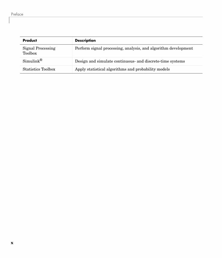
Signal Processing Toolbox
Perform signal processing, analysis, and algorithm development
Simulink® Design and simulate continuous- and discrete-time systems
Statistics Toolbox Apply statistical algorithms and probability models
Product Description

About the Author
xi
About the AuthorLennart Ljung received his PhD in Automatic Control from Lund Institute of Technology in 1974. Since 1976 he is Professor of the chair of Automatic Control in Linkoping, Sweden, and is currently Director of the Center for the “Information Systems for Industrial Control and Supervision” (ISIS). He has held visiting positions at Stanford and MIT and has written several books on System Identification and Estimation. He is an IEEE Fellow, an IFAC Advisor, a member of the Royal Swedish Academy of Sciences (KVA) and of the Royal Swedish Academy of Engineering Sciences (IVA), and has received honorary doctorates from the Baltic State Technical University in St Petersburg and from Uppsala University.

Preface
xii
1 The System Identification Problem
Basic Questions About System Identification (p. 1-2)
A quick look at the issues basic to system identification.
Common Terms Used in System Identification (p. 1-4)
A glossary of common system identification terms.
Basic Information About Dynamic Models (p. 1-6)
A discussion of properties of dynamic models, and variations of model descriptions.
The Basic Steps of System Identification (p. 1-12)
A global view of the system identification process.
A Startup Identification Procedure (p. 1-14)
A qualitative look at system identification procedure.
Reading More About System Identification (p. 1-21)
References to standard texts in system identification.

1 The System Identification Problem
1-2
Basic Questions About System Identification
What is System Identification?System Identification allows you to build mathematical models of a dynamic system based on measured data.
How is that done?Essentially by adjusting parameters within a given model until its output coincides as well as possible with the measured output.
How do you know if the model is any good?A good test is to take a close look at the model’s output compared to the measured one on a data set that wasn’t used for the fit (“Validation Data”).
Can the quality of the model be tested in other ways?It is also valuable to look at what the model couldn’t reproduce in the data (“the residuals”). This should not be correlated with other available information, such as the system's input.
What models are most common?The techniques apply to very general models. Most common models are difference equations descriptions, such as ARX and ARMAX models, as well as all types of linear state-space models.
Do you have to assume a model of a particular type?For parametric models, you have to specify the structure. This could be as easy as just selecting a single integer, the model order, or may involve several choices.If you just assume that the system is linear, you can directly estimate its impulse or step response using Correlation Analysis or its frequency response using Spectral Analysis. This allows useful comparisons with other estimated models.
What does the System Identification Toolbox contain?It contains all the common techniques to adjust parameters in all kinds of linear models. It also allows you to examine the models’ properties, and to check if they are any good, as well as to preprocess and polish the measured data.

Basic Questions About System Identification
1-3
Isn’t it a big limitation to work only with linear models?No, actually not. Many common model nonlinearities are such that the measured data should be nonlinearly transformed (like squaring a voltage input if you think that it’s the power that is the stimuli). Use physical insight about the system you are modeling and try out such transformations on models that are linear in the new variables, and you will cover a lot!
How do I get started?If you are a beginner, browse through Chapter 2, “The Graphical User Interface.” Then try out a couple of the data sets that come with the toolbox. Use the graphical user interface (GUI) and check out the built-in help functions to understand what you are doing.
Is this really all there is to System Identification?Actually, there is a huge amount written on the subject. Experience with real data is the driving force to understand more. It is important to remember that any estimated model, no matter how good it looks on your screen, has only picked up a simple reflection of reality. Surprisingly often, however, this is sufficient for rational decision making.
1 The System Identification Problem
1-4
Common Terms Used in System Identification This section defines some of the terms that are frequently used in System Identification:
• Estimation Data is the data set that is used to fit a model to data. In the GUI this is the same as the Working Data.
• Validation Data is the data set that is used for model validation purposes. This includes simulating the model for these data and computing the residuals from the model when applied to these data.
• Model Views are various ways of inspecting the properties of a model. They include looking at zeros and poles, transient and frequency response, and similar things.
• Data Views are various ways of inspecting properties of data sets. A most common and useful thing is just to plot the data and scrutinize it. So-called outliers could be detected then. These are unreliable measurements, perhaps arising from failures in the measurement equipment. The frequency contents of the data signals, in terms of periodograms or spectral estimates, are also most revealing to study.
• Model Sets or Model Structures are families of models with adjustable parameters. Parameter Estimation amounts to finding the “best” values of these parameters. The System Identification problem amounts to finding both a good model structure and good numerical values of its parameters.
• Parametric Identification Methods are techniques to estimate parameters in given model structures. Basically it is a matter of finding (by numerical search) those numerical values of the parameters that give the best agreement between the model’s (simulated or predicted) output and the measured one.
• Nonparametric Identification Methods are techniques to estimate model behavior without necessarily using a given parameterized model set. Typical nonparametric methods include Correlation Analysis, which estimates a system’s impulse response, and Spectral Analysis, which estimates a system’s frequency response.

Common Terms Used in System Identification
1-5
• Model Validation is the process of gaining confidence in a model. Essentially this is achieved by “twisting and turning” the model to scrutinize all aspects of it. Of particular importance is the model’s ability to reproduce the behavior of the validation data sets. Thus it is important to inspect the properties of the residuals from the model when applied to the validation data.
1 The System Identification Problem
1-6
Basic Information About Dynamic ModelsSystem Identification is about building dynamic models. Some knowledge about such models is therefore necessary for successful use of the toolbox. The topic is treated in several places in Chapter 3, “Tutorial.” Also, there is a wide range of textbooks available for introductory and in-depth studies. For basic use of the toolbox, it is sufficient to have quite superficial insights about dynamic models. This section describes such a basic level of knowledge.
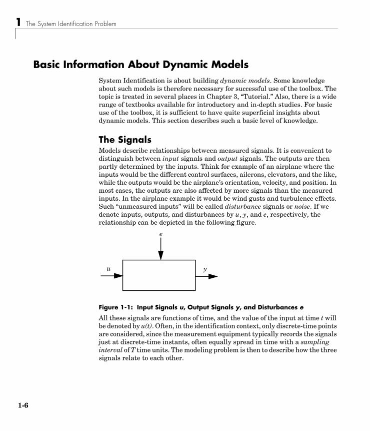
The SignalsModels describe relationships between measured signals. It is convenient to distinguish between input signals and output signals. The outputs are then partly determined by the inputs. Think for example of an airplane where the inputs would be the different control surfaces, ailerons, elevators, and the like, while the outputs would be the airplane’s orientation, velocity, and position. In most cases, the outputs are also affected by more signals than the measured inputs. In the airplane example it would be wind gusts and turbulence effects. Such ‘‘unmeasured inputs’’ will be called disturbance signals or noise. If we denote inputs, outputs, and disturbances by u, y, and e, respectively, the relationship can be depicted in the following figure.
Figure 1-1: Input Signals u, Output Signals y, and Disturbances e
All these signals are functions of time, and the value of the input at time t will be denoted by u(t). Often, in the identification context, only discrete-time points are considered, since the measurement equipment typically records the signals just at discrete-time instants, often equally spread in time with a sampling interval of T time units. The modeling problem is then to describe how the three signals relate to each other.
y
e
u
Basic Information About Dynamic Models
1-7
The Basic Dynamic ModelThe basic relationship is the linear difference equation. An example of such an equation is the following one.
Such a relationship tells us, for example, how to compute the output y(t) if the input is known and the disturbance can be ignored.
The output at time t is thus computed as a linear combination of past outputs and past inputs. It follows, for example, that the output at time t depends on the input signal at many previous time instants. This is what the word dynamic refers to. The identification problem is then to use measurements of u and y to figure out:
• The coefficients in this equation (i.e., -1.5, 0.7, etc.).
• How many delayed outputs to use in the description (two in the example:
y(t-T) and y(t-2T)).
• The time delay in the system is (2T in the example: you see from the second equation that it takes 2T time units before a change in u will affect y).
• How many delayed inputs to use (two in the example: u(t-2T) and u(t-3T)). The number of delayed inputs and outputs are usually referred to as the model order(s).
Variants of Model DescriptionsThe model given above is called an ARX model. There are a handful of variants of this model known as Output-Error (OE) models, ARMAX models, FIR models, and Box-Jenkins (BJ) models. These are described later on in the manual. At a basic level it is sufficient to think of them as variants of the ARX model allowing also a characterization of the properties of the disturbances e.
Linear state-space models are also easy to work with. See the next page for some basic definitions. The essential structure variable is just a scalar: the model order. This gives just one knob to turn when searching for a suitable model description.
y t( ) 1.5y t T–( )– 0.7y t 2T–( )+ 0.9u t 2T–( ) 0.5u t 3T–( )+= ARX( )
y t( ) 1.5y t T–( ) 0.7y t 2T–( )– 0.9u t 2T–( ) 0.5u t 3T–( )+ +=
1 The System Identification Problem
1-8
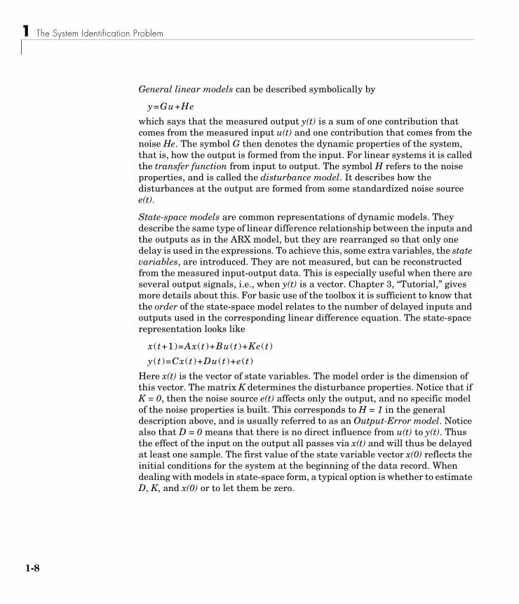
General linear models can be described symbolically by
y=Gu+He
which says that the measured output y(t) is a sum of one contribution that comes from the measured input u(t) and one contribution that comes from the noise He. The symbol G then denotes the dynamic properties of the system, that is, how the output is formed from the input. For linear systems it is called the transfer function from input to output. The symbol H refers to the noise properties, and is called the disturbance model. It describes how the disturbances at the output are formed from some standardized noise source e(t).
State-space models are common representations of dynamic models. They describe the same type of linear difference relationship between the inputs and the outputs as in the ARX model, but they are rearranged so that only one delay is used in the expressions. To achieve this, some extra variables, the state variables, are introduced. They are not measured, but can be reconstructed from the measured input-output data. This is especially useful when there are several output signals, i.e., when y(t) is a vector. Chapter 3, “Tutorial,” gives more details about this. For basic use of the toolbox it is sufficient to know that the order of the state-space model relates to the number of delayed inputs and outputs used in the corresponding linear difference equation. The state-space representation looks like
x(t+1)=Ax(t)+Bu(t)+Ke(t)
y(t)=Cx(t)+Du(t)+e(t)
Here x(t) is the vector of state variables. The model order is the dimension of this vector. The matrix K determines the disturbance properties. Notice that if K = 0, then the noise source e(t) affects only the output, and no specific model of the noise properties is built. This corresponds to H = 1 in the general description above, and is usually referred to as an Output-Error model. Notice also that D = 0 means that there is no direct influence from u(t) to y(t). Thus the effect of the input on the output all passes via x(t) and will thus be delayed at least one sample. The first value of the state variable vector x(0) reflects the initial conditions for the system at the beginning of the data record. When dealing with models in state-space form, a typical option is whether to estimate D, K, and x(0) or to let them be zero.
Basic Information About Dynamic Models
1-9
How to Interpret the Noise SourceIn many cases of system identification, the effects of the noise on the output are insignificant compared to those of the input. With good signal-to-noise ratios (SNR), it is less important to have an accurate disturbance model. Nevertheless it is important to understand the role of the disturbances and the noise source e(t), whether it appears in the ARX model or in the general descriptions given above.
There are three aspects of the disturbances that should be stressed:
• Understanding white noise
• Interpreting the noise source
• Using the noise source when working with the model
These aspects are discussed one by one.
How can we understand white noise? From a formal point of view, the noise source e will normally be regarded as white noise. This means that it is entirely unpredictable. In other words, it is impossible to guess the value of e(t) no matter how accurately we have measured past data up to time t-1.
How can we interpret the noise source? The actual disturbance contribution to the output, H e, has real significance. It contains all the influences on the measured y, known and unknown, that are not contained in the input u. It explains and captures the fact that even if an experiment is repeated with the same input, the output signal will typically be somewhat different. However, source of the noise. e need not have a physical significance. In the airplane example mentioned earlier, the disturbance effects are wind gusts and turbulence. Describing these as arising from a white noise source via a transfer function H, is just a convenient way of capturing their character.
How can we deal with the noise source when using the model? If the model is used just for simulation, i.e., the responses to various inputs are to be studied, then the disturbance model plays no immediate role. Since the noise source e(t) for new data will be unknown, it is taken as zero in the simulations, so as to study the effect of the input alone (a noise-free simulation). Making another simulation with e being arbitrary white noise will reveal how reliable the result of the simulation is, but it will not give a more accurate simulation result for the actual system’s response. It is a different thing when the model is used for prediction: Predicting future outputs from inputs and previously measured outputs means that also future disturbance contributions have to be predicted.
1 The System Identification Problem
1-10
A known, or estimated, correlation structure (which really is the disturbance model H) for the disturbances will allow predictions of future disturbances, based on the previously measured values.
The need and use of the noise model can be summarized as follows:
• It is, in most cases, required to obtain a better estimate for the dynamics, G.
• It indicates how reliable noise-free simulations are.
• It is required for reliable predictions and stochastic control design.
Terms to Characterize the Model PropertiesThe properties of an input-output relationship like the ARX model follow from the numerical values of the coefficients and the number of delays used. This is however a fairly implicit way of talking about the model properties. Instead a number of different terms are used in practice:
Impulse ResponseThe impulse response of a dynamic model is the output signal that results when the input is an impulse, i.e., u(t) is zero for all values of t except t=0, where u(0)=1. It can be computed as in the equation following (ARX), by letting t be equal to 0, T, 2T, ... and taking y(-T)=y(-2T)=0 and u(0)=1.
Step ResponseThe step response is the output signal that results from a step input, i.e., u(t) is zero for negative values of t and equal to one for positive values of t. The impulse and step responses together are called the model’s transient response.
Frequency ResponseThe frequency response of a linear dynamic model describes how the model reacts to sinusoidal inputs. If we let the input u(t) be a sinusoid of a certain frequency, then the output y(t) will also be a sinusoid of this frequency. The amplitude and the phase (relative to the input) will however be different. This frequency response is most often depicted by two plots: one that shows the amplitude change as a function of the sinusoid’s frequency and one that shows the phase shift as function of frequency. This is known as a Bode plot.
Basic Information About Dynamic Models
1-11
Zeros and PolesThe zeros and the poles are equivalent ways of describing the coefficients of a linear difference equation like the ARX model. The poles relate to the “output side” and the zeros relate to the “input side” of this equation. The number of poles (zeros) is equal to the number of sampling intervals between the most and least delayed output (input). In the ARX example in the beginning of this section, there are consequently two poles and one zero.
1 The System Identification Problem
1-12
The Basic Steps of System IdentificationThe System Identification problem is to estimate a model of a system based on observed input-output data. Several ways to describe a system and to estimate such descriptions exist. This section gives a brief account of the most important approaches.
The procedure to determine a model of a dynamical system from observed input-output data involves three basic ingredients:
• The input-output data
• A set of candidate models (the model structure)
• A criterion to select a particular model in the set, based on the information in the data (the identification method)
The identification process amounts to repeatedly selecting a model structure, computing the best model in the structure, and evaluating this model’s properties to see if they are satisfactory. The cycle can be itemized as follows:
1 Design an experiment and collect input-output data from the process to be identified.
2 Examine the data. Polish it so as to remove trends and outliers, and select useful portions of the original data. Possibly apply filtering to enhance important frequency ranges.
3 Select and define a model structure (a set of candidate system descriptions) within which a model is to be found.
4 Compute the best model in the model structure according to the input-output data and a given criterion of fit.
5 Examine the obtained model’s properties.
6 If the model is good enough, then stop; otherwise go back to Step 3 to try another model set. Possibly also try other estimation methods (Step 4) or work further on the input-output data (Steps 1 and 2).
The Basic Steps of System Identification
1-13
The System Identification Toolbox offers several functions for each of these steps.
For Step 2 there are routines to plot data, filter data, and remove trends in data, as well as to resample and reconstruct missing data.
For Step 3 the System Identification Toolbox offers a variety of nonparametric models, as well as all the most common black-box input-output and state-space structures, and also general tailor-made linear state-space models in discrete and continuous time.
For Step 4 general prediction error (maximum likelihood) methods, as well as instrumental variable methods and sub-space methods are offered for parametric models, while basic correlation and spectral analysis methods are used for nonparametric model structures.
To examine models in Step 5, many functions allow the computation and presentation of frequency functions and poles and zeros, as well as simulation and prediction using the model. Functions are also included for transformations between continuous-time and discrete-time model descriptions and to formats that are used in other toolboxes such as the Control System Toolbox and the Signal Processing Toolbox.
1 The System Identification Problem
1-14
A Startup Identification ProcedureThere are no standard and secure routes to good models in System Identification. Given the number of possibilities, it is easy to get confused about what to do, what model structures to test, and so on. This section describes one route that often works well, but there are no guarantees. The steps refer to functions within the GUI, but you can also go through them in command mode. For the basic commands, see Chapter 4, “Function Reference.”
Step 1: Looking at the Data Plot the data. Look at it carefully. Try to see the dynamics with your own eyes. Can you see the effects in the outputs of the changes in the input? Can you see nonlinear effects, like different responses at different levels, or different responses to a step up and a step down? Are there portions of the data that appear to be “messy” or carry no information? Use this insight to select portions of the data for estimation and validation purposes.
Do physical levels play a role in your model? If not, detrend the data by removing their mean values. The models will then describe how changes in the input give changes in output, but not explain the actual levels of the signals. This is the normal situation.
The default situation, with good data, is that you detrend by removing means, and then select the first half or so of the data record for estimation purposes, and use the remaining data for validation. This is what happens when you select Preprocess -> Quickstart in the main ident window.
Step 2: Getting a Feel for the DifficultiesSelect Estimate -> Quickstart in the main ident window. This will compute and display the spectral analysis estimate and the correlation analysis estimate, as well as a fourth-order ARX model with a delay estimated from the correlation analysis and a default order state-space model computed by n4sid. This gives three plots. Look at the agreement between
• Spectral analysis estimate and the ARX and state-space models’ frequency functions
• Correlation analysis estimate and the ARX and state-space models’ transient responses
A Startup Identification Procedure
1-15
• Measured validation data output and the ARX and state-space models’ simulated outputs
If these agreements are reasonable, the problem is not so difficult, and a relatively simple linear model will do a good job. Some fine tuning of model orders, and noise models have to be made, and you can proceed to Step 4. Otherwise go to Step 3.
Step 3: Examining the DifficultiesThere may be several reasons why the comparisons in Step 2 did not look good. This section discusses the most common ones, and how they can be handled.
Model UnstableThe ARX or state-space model may turn out to be unstable, but could still be useful for control purposes. Change to a 5- or 10-step ahead prediction instead of simulation in the Model Output View.
Feedback in DataIf there is feedback from the output to the input, due to some regulator, then the spectral and correlations analysis estimates are not reliable. Discrepancies between these estimates and the ARX and state-space models can therefore be disregarded in this case. In the Model Residuals View of the parametric models, feedback in data can also be visible as correlation between residuals and input for negative lags.
Disturbance ModelIf the state-space model is clearly better than the ARX model at reproducing the measured output, this is an indication that the disturbances have a substantial influence, and it will be necessary to model them carefully.
Model OrderIf a fourth-order model does not give a good Model Output plot, try eighth-order. If the fit clearly improves, it follows that higher order models will be required, but that linear models could be sufficient.
Additional Inputs If the Model Output fit has not significantly improved by the tests so far, think over the physics of the application. Are there more signals that have been, or
1 The System Identification Problem
1-16
could be, measured that might influence the output? If so, include these among the inputs and try again a fourth-order ARX model from all the inputs. (Note that the inputs need not at all be control signals, anything measurable, including disturbances, should be treated as inputs).
Nonlinear Effects If the fit between measured and model output is still bad, consider the physics of the application. Are there nonlinear effects in the system? In that case, form the nonlinearities from the measured data and add those transformed measurements as extra inputs. This could be as simple as forming the product of voltage and current measurements, if you realize that it is the electrical power that is the driving stimulus in, say, a heating process, and temperature is the output. This is of course application dependent. It does not take very much work, however, to form a number of additional inputs by reasonable nonlinear transformations of the measured ones, and just test if inclusion of them improves the fit.
Still Problems?If none of these tests leads to a model that is able to reproduce the validation data reasonably well, the conclusion might be that a sufficiently good model cannot be produced from the data. There may be many reasons for this. It may be that the system has some quite complicated nonlinearities, which cannot be realized on physical grounds. In such cases, nonlinear, black-box models could be a solution. Among the most used models of this character are the Artificial Neural Networks (ANN).
Another important reason is that the data simply do not contain sufficient information, e.g., due to bad signal to noise ratios, large and nonstationary disturbances, varying system properties, etc.
Otherwise, use the insights of which inputs to use and which model orders to expect and proceed to Step 4.
Step 4: Fine Tuning Orders and Disturbance Structures For real data there is no such thing as a “correct model structure.” However, different structures can give quite different model quality. The only way to find this out is to try out a number of different structures and compare the
A Startup Identification Procedure
1-17
properties of the models obtained. There are a few things to look for in these comparisons.
Fit Between Simulated and Measured Output Keep the Model Output View open and look at the fit between the model’s simulated output and the measured one for the validation data. Formally, you could pick that model, for which this number is the highest. In practice, it is better to be more pragmatic, and also take into account the model complexity and whether the important features of the output response are captured.
Residual Analysis Test You should require of a good model that the cross correlation function between residuals and input does not go significantly outside the confidence region. Otherwise there is something in the residuals that originate from the input, and has not been properly taken care of by the model. A clear peak at lag k shows that the effect from input u(t-k) on y(t) is not correctly described. A rule of thumb is that a slowly varying cross correlation function outside the confidence region is an indication of too few poles, while sharper peaks indicate too few zeros or wrong delays.
Pole Zero Cancellations If the pole-zero plot (including confidence intervals) indicates pole-zero cancellations in the dynamics, this suggests that lower order models can be used. In particular, if it turns out that the orders of ARX models have to be increased to get a good fit, but that pole-zero cancellations are indicated, then the extra poles are just introduced to describe the noise. Then try ARMAX, OE, or BJ model structures with an A or F polynomial of an order equal to that of the number of noncanceled poles.
What Model Structures Should be Tested? Well, you can spend any amount of time to check out a very large number of structures. It often takes just a few seconds to compute and evaluate a model in a certain structure, so that you should have a generous attitude to the testing. However, experience shows that when the basic properties of the system’s behavior have been picked up, it is not much use to fine- tune orders ad absurdum just to press the fit by fractions of percents.
Many ARX models: There is a very cheap way of testing many ARX structures simultaneously. Enter in the Orders text field many combinations of orders,

1 The System Identification Problem
1-18
using the colon (:) notation. You can also click the Order Selection button. When you select Estimate, models for all combinations (easily several hundreds) are computed and their (prediction error) fit to validation data is shown in a special plot. By clicking in this plot the best models with any chosen number of parameters will be inserted into the Model Board, and evaluated as desired.
Many state-space models: A similar feature is also available for black-box state-space models, estimated using n4sid. When a good order has been found, try the PEM estimation method, which often improves on the accuracy.
ARMAX, OE, and BJ models: Once you have a feel for suitable delays and dynamics orders, it is often useful to try out ARMAX, OE, and/or BJ with these orders and test some different orders for the disturbance transfer functions (C and D). Especially for poorly damped systems, the OE structure is suitable.
There is a quite extensive literature on order and structure selection, and anyone who would like to know more should consult the references.
Multivariable Systems Systems with many input signals and/or many output signals are called multivariable. Such systems are often more challenging to model. In particular systems with several outputs could be difficult. A basic reason for the difficulties is that the couplings between several inputs and outputs lead to more complex models. The structures involved are richer and more parameters will be required to obtain a good fit.
Available ModelsThe System Identification Toolbox as well as the GUI handle general, linear multivariable models. All models mentioned earlier are supported in the single-output, multiple-input case. For multiple outputs, ARX models and state-space models are covered. Multiple-output ARMAX and OE models are covered via state-space representations: ARMAX corresponds to estimating the K-matrix, while OE corresponds to fixing K to zero. (These are options in the GUI model order editor.)
Generally speaking, it is preferable to work with state-space models in the multivariable case, since the model structure complexity is easier to deal with. It is essentially just a matter of choosing the model order.
A Startup Identification Procedure
1-19
Working with Subsets of the Input-Output ChannelsIn the process of identifying good models of a system, it is often useful to select subsets of the input and output channels. Partial models of the system’s behavior will then be constructed. It might not, for example, be clear if all measured inputs have a significant influence on the outputs. That is most easily tested by removing an input channel from the data, building a model for how the output(s) depends on the remaining input channels, and checking if there is a significant deterioration in the model output’s fit to the measured one. See also the discussion under Step 3 above.
Generally speaking, the fit gets better when more inputs are included and often gets worse when more outputs are included. To understand the latter fact, you should realize that a model that has to explain the behavior of several outputs has a tougher job than one that must just account for a single output. If you have difficulties obtaining good models for a multioutput system, it might be wise to model one output at a time, to find out which are the difficult ones to handle.
Models that are just to be used for simulations could very well be built up from single-output models, for one output at a time. However, models for prediction and control will be able to produce better results if constructed for all outputs simultaneously. This follows from the fact that knowing the set of all previous output channels gives a better basis for prediction than just knowing the past outputs in one channel. Also, for systems where the different outputs reflect similar dynamics, using several outputs simultaneously will help estimating the dynamics.
Some Practical AdviceBoth the GUI and command-line operation will do useful bookkeeping for you, handling different channels. You could follow the steps of this agenda:
• Import data and create a data set with all input and output channels of interest. Do the necessary preprocessing of this set in terms of detrending, etc., and then select a Validation Data set with all channels.
• Then select a Working Data set with all channels, and estimate state-space models of different orders using n4sid for these data. Examine the resulting model primarily using the Model Output view.
• If it is difficult to get a good fit in all output channels or you would like to investigate how important the different input channels are, construct new data sets using subsets of the original input/output channels. Use the menu

1 The System Identification Problem
1-20
item Preprocess -> Select Channels for this. Don’t change the validation data. The GUI will keep track of the input and output channels. It will “do the right thing” when evaluating the channel-restricted models using the validation data. It might also be appropriate to see if improvements in the fit are obtained for various model types, built for one output at a time.
• If you decide on a multioutput model, it is often easiest to use state-space models. Use n4sid as a primary tool and try out pem when a good order has been found.
Reading More About System Identification
1-21
Reading More About System IdentificationThere is substantial literature on System Identification. The following textbook deals with identification methods from a perspective like this toolbox’s, and also describes methods for physical modeling:
• Ljung, L., and T. Glad, Modeling of Dynamic Systems, Prentice Hall, Englewood Cliffs, N.J., 1994.
For more details about the algorithms and theories of identification,
• Ljung, L., System Identification – Theory for the User, Prentice Hall, Upper Saddle River, N.J., 2nd edition, 1999.
• Söderström, T., and P. Stoica, System Identification, Prentice Hall International, London. 1989.
For more about system and signals,
• Oppenheim, J., and A.S. Willsky, Signals and Systems, Prentice Hall, Englewood Cliffs, N.J., 1985.
The following textbook deals with the underlying numerical techniques for parameter estimation:
• Dennis, J.E., Jr., and R.B. Schnabel, Numerical Methods for Unconstrained Optimization and Nonlinear Equations, Prentice Hall, Englewood Cliffs, N.J., 1983.

1 The System Identification Problem
1-22

2The Graphical User Interface
The Big Picture (p. 2-2) A quick overview of the Ident GUI
Handling Data (p. 2-7) Importing, preprocessing, and viewing data
Estimating Models (p. 2-17) A discussion of direct and parametric identification methods
Examining Models (p. 2-33) Examining, comparing, and validating identified models using frequency and transient responses, poles and zeros, and model outputs and residuals
Some Further GUI Topics (p. 2-41) Additional topics about the Ident GUI, including troubleshooting and customizing plots, reconfiguring the default layout, and limitations of the Ident GUI
2 The Graphical User Interface
2-2
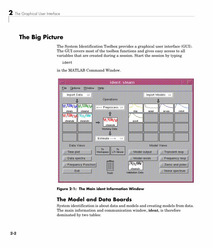
The Big PictureThe System Identification Toolbox provides a graphical user interface (GUI). The GUI covers most of the toolbox functions and gives easy access to all variables that are created during a session. Start the session by typing
ident
in the MATLAB Command Window.
Figure 2-1: The Main ident Information Window
The Model and Data BoardsSystem identification is about data and models and creating models from data. The main information and communication window, ident, is therefore dominated by two tables:
The Big Picture
2-3
• A table over available data sets, each represented by an icon
• A table over created models, each represented by an icon
These tables are referred to as the model board and the data board in this chapter. You enter data sets into the data board by
• Opening earlier saved sessions
• Importing them from the MATLAB workspace
• Creating them by detrending, filtering, transforming, and selecting subsets of another data set in the data board
Imports are handled under the menu Data while creation of new data sets is handled under the menu Preprocess. “Handling Data” on page 2-7 deals with this in more detail. The GUI supports three kinds of data objects for estimation. Both objects and vector- or matrix-valued signals can be imported:
• Time-domain input/output signals (in the iddata object format). These are marked by a white background color.
• Frequency-domain input/output signals (in the iddata object format). These are marked by a light green background color.
• Frequency functions (in the idfrd object format). These are estimates of the system’s frequency function (frequency response), obtained either by special data acquisition equipment (frequency analyzers) or as estimates from measured input-output data. These data sets are marked by a light brown background color.
You enter the models into the summary board by
• Opening earlier saved sessions
• Importing them from the MATLAB workspace
• Estimating them from data
Imports are handled under the menu Models, while all the different estimation schemes are reached under the menu Estimate. More about this in “Estimating Models” on page 2-17.
You can rearrange the data and model boards by dragging and dropping. More boards open automatically when necessary or when asked for (under menu Options).

2 The Graphical User Interface
2-4
The Working DataAll data sets and models are created from the working data set. This is the data that is given in the center of the ident window. To change the working data set, drag and drop any data set from the data board on the working data icon.
The ViewsBelow the data and model boards are buttons for different views. These control what aspects of the data sets and models you would like to examine, and are described in more detail in “Handling Data” on page 2-7 and in “Examining Models” on page 2-33. To select a data set or a model so that its properties are displayed, click its icon. A selected object is marked by a thicker line in the icon. To clear it, click again. You can examine an arbitrary number of data/model objects simultaneously. To obtain more information about an object, double-click (or right-click or Ctrl+click) its icon.
The Validation DataThe two model views Model Output and Model Residuals illustrate model properties when applied to the validation data set. This is the set marked in the box below these two views. To change the validation data, drag and drop any data set from the data board on the validation data icon.
It is good and common practice in identification to evaluate an estimated model’s properties using a “fresh” data set, that is, one that was not used for the estimation. It is thus good advice to let the validation data be different from the working data, but they should of course be compatible with these.
The Work FlowYou start by importing data (under menu Data); you examine the data set using the Data Views. You probably remove the means from the data and select subsets of data for estimation and validation purposes using the items in the menu Preprocess. You then continue to estimate models, using the possibilities under the menu Estimate, perhaps first doing a quickstart. You examine the obtained models with respect to your favorite aspects using the different Model Views. The basic idea is that any selected view shows the properties of all selected models at any time. This function is “live” so models and views can be checked in and out at will in an online fashion. You select/deselect a model by clicking its icon.
The Big Picture
2-5
Inspired by the information you gain from the plots, you continue to try out different model structures (model orders) until you find a model you are satisfied with.
Management AspectsDiary: It is easy to forget what you have been doing. By double-clicking a data/model icon, you get a complete diary of how this object was created, along with other key information. At this point you can also add comments and change the name of the object and its color.
Layout: To have a good overview of the created models and data sets, it is good practice to try rearranging the icons by dragging and dropping. In this way models corresponding to a particular data set can be grouped together, etc. You can also open new boards (Options -> Extra model/data boards) to further rearrange the icons. These can be dragged across the screen between different windows. The extra boards are also equipped with notepads for your comments.
Sessions: The model and data boards with all models and data sets together with their diaries can be saved (under menu item File) at any point, and reloaded later. This is the counterpart of save/load workspace in the command-driven MATLAB. The four most recent sessions are listed under File for immediate open.
Cleanliness: The boards will hold an arbitrary number of models and data sets (by creating clones of the board when necessary). It is however advisable to clear (delete) models and data sets that no longer are of interest. Do that by dragging the object to the trash can icon. (Double-clicking the trash can will open it. You can retrieve its contents.) Empty the trash can if you run into memory problems.
Warnings: Several messages from the underlying computations can show up in warning dialog boxes. You can turn off these warnings using an item in the Options menu.
Window Culture: Dialog and plot windows are best managed by the GUI’s close function (submenu item under File menu). Alternatively, select Close or select/clear the corresponding View box. It is generally not suitable to iconify the windows — the GUI’s handling and window management system is usually a better alternative.
2 The Graphical User Interface
2-6
Workspace VariablesThe models and data sets created within the GUI are normally not available in the MATLAB workspace. Indeed, the workspace is not at all littered with variables during the sessions with the GUI. You can, however, export the variables to the workspace at any time, by dragging and dropping the object icon on the To Workspace box. They will then carry the name in the workspace that marked the object icon at the time of export. You can work with the variables in the workspace, using any MATLAB commands, and then perhaps import modified versions back into the GUI. Note that models and data are exported as the toolbox objects idmodel, idfrd, and iddata. For how to extract information and work with these objects, see “Data Representation” on page 3-19 and “Model Conversions” on page 4-6.
The GUI’s names of data sets and models are suggested by default procedures. Normally, you can enter any other name of your choice at the time of creation of the variable. Names can be changed (after double-clicking the icon) at any time. Unlike the workspace situation, two GUI objects can carry the same name (i.e., the same string in their icons).
Help TextsThe GUI contains some 100 help texts that are accessible in a nested fashion when required. The main ident window contains general help topics under the Help menu. This is also the case for the various plot windows. In addition, every dialog box has a Help button for current help and advice.
Handling Data
2-7
Handling Data
Data Representation In the System Identification Toolbox, signals and observed data are represented as column vectors, for example:
The entry in row number k, i.e., u(k), will then be the signal’s value at sampling instant number k. It is generally assumed in the toolbox that data is sampled at equidistant sampling times, and the sampling interval T is supplied as a specific argument.
For frequency-domain data, u(k) is interpreted as the Fourier transform of the input at frequency w(k), where the frequency vector w is defined along with the input.
We generally denote the input to a system by the letter u and the output by y. If the system has several input channels, the input data is represented by a matrix, where the columns are the input signals in the different channels.
The same holds for systems with several output channels.
The observed input-output data record is represented in the System Identification Toolbox by the iddata object that is created from the input and output signals by
Data = iddata(y,u,Ts)
where Ts is the sampling time. For frequency-domain data, the object is defined as
Data = iddata(y,u,Ts,'Domain','Frequency','Freq',w)
where w is the vector of frequencies.
u
u 1( )u 2( )……
u N( )
=
u u1 u2 … um=
2 The Graphical User Interface
2-8
The iddata object can also be created from the input and output signals when the data is inserted into the GUI.
Another data representation that can be used for model estimation is frequency responses (frequency functions). This consists of the frequency response from input to output G(w) (which the transfer function evaluated on the unit circle or the imaginary axis). The frequency function G(w) is a complex number, whose absolute value describes how a sinusoid of frequency w is amplified by the system, and whose argument (phase) described how the same signal is shifted (phase-lagged) by the system. Frequency response data is contained in the idfrd object:
Datfr = idfrd(G,w,Ts)
Also idfrd objects can be created from the basic signals when they are imported into the GUI.
Getting Data into the GUITo bring data into the GUI, select the menu Import Data in the main GUI window. This gives you three choices:
• Time-domain data
• Frequency-domain data (covers also frequency response data)
• Data object
Depending on what you choose, slightly different dialog windows open up.
For input/output data, the information about a data set that should be supplied to the GUI is as follows:
• The input and output signals
• The name you give to the data set
• The sampling interval Ts. (Ts = 0 denotes time continuous data, which then must be frequency domain.)
For frequency-domain data, you also have to supply the
• Frequency vector
In addition to this mandatory information, you can add further properties that will help in the bookkeeping:
Handling Data
2-9
• The starting time for the sampling (for frequency-domain data, enter instead the frequency unit, Hz or rad/s)
• Input and output channel names
• Input and output channel units
• Periodicity and intersample behavior of the input
• Data notes: These are notes for your own information and bookkeeping that will follow the data and all models created from it.
Note that the sampling interval and the input intersample properties are relevant also for frequency-domain data, since they determine how to interpret the information in the data.
In the case of frequency-response data, you have to enter
• The response function, either as a vector of complex values or as amplitude and phase
• The corresponding vector of frequencies
• The underlying sampling interval Ts. Use Ts = 0 if the response corresponds to a continuous time system.
If the system has nu inputs and ny outputs, and the response is given at nf frequencies, the response function is an ny-by-nu-by-nf 3-D array. In this case also, you can supply bookkeeping information as above.
As you select the menu Data Import and choose the relevant item, a dialog box will open where you can enter the information listed above.

2 The Graphical User Interface
2-10
Figure 2-2: The Dialog for Importing Data into the GUI
Clicking More makes more fields visible.
For the time-domain data case, the fields are as follows:
Input and Output: Enter the variable names of the input and output respectively. These should be variables in your MATLAB workspace, so you might have to load some disk files first.
Actually, you can enter any MATLAB expressions in these fields, and they will be evaluated to compute the input and the output before inserting the data into the GUI.
Data name: Enter the name of the data set to be used by the GUI. This name can be changed later on.
Handling Data
2-11
Starting time and Sampling interval: Fill these out for correct time and frequency scales in the plots.
On the extra page you can optionally fill out
Channel names: Enter strings for the different input and output channel names. Separate the strings by commas. The number of names must be equal to the number of channels. If these entries are not filled out, default names, for example, y1, y2, ..., u1, u2, ..., are used.
Channel units: Enter, in analogous format, the units in which the measurements are made. These will follow to all models built from data, but are used only for plot information.
Period: If the input is periodic, enter the period length. Inf means a nonperiodic input, which is the default.
Intersample: Choose the intersample behavior of the input as ZOH (zero-order hold, i.e., the input signal is piecewise constant between the samples) or FOH (first-order hold, i.e., the input signal is piecewise linear between the samples) or BL (band-limited, i.e., the continuous time input signal has no power above the Nyquist frequency). ZOH is the default.
The box at the bottom is for Notes, where you can enter any text you want to accompany the data for bookkeeping purposes.
Finally, select Import to insert the data into the GUI. When no more data sets are to be inserted, select Close to close the dialog box. Selecting Reset will empty all the fields of the box.
The procedure just described creates an iddata object, with all its properties (or correspondingly an idfrd object, in the frequency-response data case.) If you already have an iddata or idfrd object available in the workspace, you can import that directly by selecting the item Data Object in the menu Import Data.
Taking a Look at the DataThe first thing to do after inserting the data set into the data board is to examine it. By selecting the Data View item Time plot, a plot of the input and output signals is shown for the data sets that are selected. You select/clear the data sets by clicking them. For multivariable data, you can choose the different combinations of input and output signals under the menu item Channel in the
2 The Graphical User Interface
2-12
plot window. Using the zoom function (drawing rectangles with the left mouse button down), you can examine different portions of the data in more detail.
To examine the frequency contents of the data, select the Data View item Data spectra. The function is analogous to Time plot, but the signals’ spectra are shown instead. By default the periodograms of the data are shown, i.e., the absolute square of the Fourier transforms of the data. You can change the plot to any chosen frequency range and a number of different ways of estimating spectra, using the Options menu item in the spectra window.
The purpose of examining the data in these ways is to find out if there are portions of the data that are not suitable for identification, if the information contents of the data are suitable in the interesting frequency regions, and if the data has to be preprocessed in some way before it can be used for estimation.
Another way of examining data is the Data View item Frequency Function. For a frequency response data set this shows the amplitude and phase of the frequency function. For time- or frequency-domain input/output data, this view shows the empirical transfer function estimate (etfe) based on the data.
Preprocessing DataThe menu Preprocess gives access to a number of methods to modify and transform the data sets on the data board. The commands are applied to the currently chosen Working Data. The actual menu of choices depends on this data set. Not all choices are applicable to all kinds of data sets.
DetrendingDetrending the data involves removing the mean values or linear trends from the signals (the means and the linear trends are then computed and removed from each signal individually). You access this function under the menu Preprocess by selecting item Remove Means or Remove Trends. More advanced detrending, such as removing piecewise linear trends or seasonal variations, cannot be accessed within the GUI. We generally recommend that you remove at least the mean values of the data before the estimation phase. There are, however, situations when it is not advisable to remove the sample means. It could be, for example, that the physical levels are built into the underlying model, or that integrations in the system must be handled with the right level of the input being integrated.
Handling Data
2-13
Selecting Data RangesIt is often the case that the whole data record is not suitable for identification, due to various undesired features (missing or “bad” data, outbursts of disturbances, level changes, etc.), so that only portions of the data can be used. In any case, it is advisable to select one portion of the measured data for estimation purposes and another portion for validation purposes. The menu item Preprocess -> Select Range opens a dialog box that facilitates the selection of different data portions, by typing in the ranges, or marking them by drawing rectangles with the mouse button down.
For multivariable data it is often advantageous to start by working with just some of the input and output signals. The menu item Preprocess -> Select Channels allows you to select subsets of the inputs and outputs. This is done in such a way that the input/output numbering and names remain consistent when you evaluate data and model properties, for models covering different subsets of the data.
PrefilteringBy filtering the input and output signals through a linear filter (the same filter for all signals) you can, for example, remove drift and high-frequency disturbances in the data, which should not affect the model estimation. You do this by selecting the menu item Preprocess -> Filter in the main window. The dialog is quite analogous to that of selecting data ranges in the time domain. You mark with a rectangle in the spectral plots the intended passband or stop band of the filter, you select a button to check if the filtering has the desired effect, and then you insert the filtered data into the GUI’s data board.
Prefiltering is a good way of removing high-frequency noise in the data, and is also a good alternative to detrending (by cutting out low frequencies from the pass band). Depending on the intended model use, you can also make sure that the model concentrates on the important frequency ranges. For a model that will be used for control design, for example, the frequency band around the intended closed-loop bandwidth is of special importance.
If you intend to use the data to build models both of the system dynamics and the disturbance properties, we recommend that you do the filtering at the estimation phase. That is achieved by selecting the menu item Estimate -> Parametric Models, and then selecting the estimation Focus to be Filter. This opens the same filter dialog as above. The prefiltering will however apply only for estimating the dynamics from input to output. The disturbance model is determined from the original data.
2 The Graphical User Interface
2-14
ResamplingIf the data turns out to be sampled too fast, it can be decimated, i.e., every kth value is picked, after proper prefiltering (antialias filtering). This is obtained from menu item Preprocess -> Resample.
You can also resample at a faster sampling rate by interpolation, using the same command, and giving a resampling factor of less than one.
Transform DataThe menu item Preprocess -> Transform Data opens a dialog that allows you to transform between time- and frequency-domain input/output data and also to form frequency-response data sets from input/output data.
QuickstartThe menu item Preprocess -> Quickstart performs the following sequence of actions: It opens the Time plot Data view, removes the means from the signals, and splits these detrended data into two halves. The first one is made working data and the second one becomes validation data. All three created data sets are inserted into the data board.
Multiexperiment DataThe System Identification Toolbox allows the handling of data sets that contain several different experiments. Both estimation and validation can be applied to such data sets. This is quite useful to deal with experiments that have been conducted at different occasions but describe the same system. It is also useful to be able to keep together pieces of data that have been obtained by cutting out “informative pieces” from a long data set. Multiexperiment data can be imported and used in the GUI like any iddata object. Selecting a specific part of a multiexperiment data set is done from the menu item Preprocess -> Select Experiment. To merge several data sets in the data board (obtained, for example, by cutting out portions from other data sets) use the menu item Preprocess -> Merge Experiment.
Checklist for Data Handling• Insert data into the GUI’s Data Board.
• Plot the data and examine it carefully.
• Typically detrend the data by removing mean values.
Handling Data
2-15
• Select portions of the data for estimation and for validation. Drag and drop these data sets to the corresponding boxes in the GUI.
Simulating DataThe GUI is intended primarily for working with real data sets, and does not itself provide functions for simulating synthetic data. That has to be done in command mode, and you can use your favorite procedure in Simulink, the Signal Processing Toolbox, or any other toolbox for simulation and then insert the simulated data into the GUI as described above.
The System Identification Toolbox also has several commands for simulation. For example, see the reference pages for idinput and sim for details.
The following example shows how the ARMAX model
is simulated with a random binary input u.
% Create an ARMAX modelmodel1 = idpoly([1 -1.5 0.7],[0 1 0.5],[1 -1 0.2]);u = idinput(400,'rbs',[0 0.3]); e = randn(400,1);y = sim(model1,[u e]);
The input, u, and the output, y, can now be imported into the GUI as data, and the various estimation routines can be applied to them. If you also import the simulation model, model1, into the GUI, its properties can be compared to those of the different estimated models.
To simulate a continuous-time state-space model
with the same input, and a sampling interval of 0.1 second, do the following in the System Identification Toolbox:
A = [-1 1;-0.5 0]; B = [1; 0.5]; C = [1 0]; D = 0; K = [0.5;0.5];Model2 = idss(A,B,C,D,K,'Ts', 0) % Ts = 0 means continuous timeData = iddata([],[u e]);
y t( ) 1.5y t 1–( )– 0.7y t 2–( )+ =u t 1–( ) 0.5u t 2–( ) e t( ) e t 1–( )– 0.2e t 1–( )+ + +
x· Ax Bu Ke+ +=y Cx e+=

2 The Graphical User Interface
2-16
Data.Ts = 0.1y=sim(Model2,Data);
Estimating Models
2-17
Estimating Models
The Basics Estimating models from data is the central activity in the System Identification Toolbox. It is also the one that offers the most variety of possibilities and thus is the most demanding one for the user.
All estimation routines are accessed from the menu Estimate in the ident window. The models are always estimated using the data set that is currently in the Working Data box.
One can distinguish between two different types of estimation methods:
• Direct estimation of the impulse or the frequency response of the system. These methods are often also called nonparametric estimation methods, and do not impose any structure assumptions about the system, other than that it is linear.
• Parametric methods. A specific model structure is assumed, and the parameters in this structure are estimated using data. This opens up a large variety of possibilities, corresponding to different ways of describing the system. Dominating ways are state-space and several variants of difference equation descriptions.
Direct Estimation of the Impulse Response A linear system can be described by the impulse response , with the property that
The name derives from the fact that if the input u(t) is an impulse, i.e., u(t)=1 when t=0 and 0 when t>0, then the output y(t) will be . For a multivariable system, the impulse response will be an ny-by-nu matrix where ny is the number of outputs and nu is the number of inputs. Its i-j element thus describes the behavior of the ith output after an impulse in the jth input.
Choosing menu item Estimate -> Correlation Model opens a dialog window that lets you directly estimate the impulse response coefficients from the
gk
y t( ) gku t k–( )
k 1=
∞
∑=
y t( ) gt=gk
2 The Graphical User Interface
2-18
input/output data using so called correlation analysis. The actual method is described under the command impulse in Chapter 4, “Function Reference.” For a quick action, you can also just type the letter c in the ident window. This is the hot key for correlation analysis.
The resulting impulse response estimate is placed in the model board, under the default name imp. (You can change the name by double-clicking the model icon and then typing in the desired name in the dialog box that opens.)
The best way to examine the result is to select the Model View Transient Response. This gives a graph of the estimated response. This view offers a choice between displaying the impulse or the step response. For a multivariable system, the different channels, i.e., the responses from a certain input to a certain output, are selected under menu item Channel.
The number of lags for which the impulse response is estimated, i.e., the length of the estimated response, is determined as one of the options in the Transient Response view.
Direct Estimation of the Frequency ResponseThe frequency response of a linear system is the Fourier transform of its impulse response. This description of the system gives considerable engineering insight into its properties. The relation between input and output is often written
y(t)=G(z)u(t)+v(t)
where G is the transfer function and v is the additive disturbance. The function
as a function of (angular) frequency ω is then the frequency response or frequency function. T is the sampling interval. If you need more details on the different interpretations of the frequency response, see “The System Identification Problem” on page 3-9 or any textbook on linear systems.
The system’s frequency response is directly estimated using spectral analysis by the menu item Estimate -> Spectral Model, and then selecting the Estimate button in the dialog box that opens. The result is placed on the model board under the default name spd. The best way to examine it is to plot it using the Model View Frequency Response. This view offers a number of different options on how to graph the curves. You can also select the frequencies for
G eiωT( )
Estimating Models
2-19
which to estimate the response by specifying the number of frequencies and the spacing (linear or logarithmic) in the Spectral Model dialog box. The spectral analysis command also estimates the spectrum of the additive disturbance v(t) in the system description. This estimated disturbance spectrum is examined under the Model View item Noise Spectrum.
The spectral analysis estimate is stored as an idfrd object. If you need to work further with the estimates, you can export the model to the MATLAB workspace and retrieve the responses directly from this object or by using the nyquist or bode command. See idfrd, bode, and nyquist in Chapter 4, “Function Reference,” for more information. (Export a model by dragging and dropping it over the To Workspace icon.)
A few options that affect the spectral analysis estimate can be set in the dialog box. The most important choice is the frequency resolution. This is a number, M, (the size of the lag window) that affects the frequency resolution of the estimates. Essentially, the frequency resolution is about 2 /M radians/(sampling interval). The choice of M is a tradeoff between frequency resolution and variance (fluctuations). A large value of M gives good resolution but fluctuating and less reliable estimates. The default choice of M is good for systems that do not have very sharp resonances and may have to be adjusted for more resonant systems.
The options also offer a choice between the Blackman-Tukey windowing method spa (which is the default); a variant with frequency dependent resolution, spafdr; and a method based on smoothing direct Fourier transforms, etfe. etfe has an advantage for highly resonant systems in that it is more efficient for large values of M. It however has the drawbacks that it requires linearly spaced frequency values, does not estimate the disturbance spectrum, and does not provide confidence intervals. The actual methods are described in more detail in Chapter 4, “Function Reference,” under spa, spafdr, and etfe. To obtain the spectral analysis model for the current settings of the options, you can just type the hot key s in the ident window.
Estimation of Simple Process ModelThe System Identification Toolbox allows you to estimate simple continuous-time process models characterizing the static gain, dominating time constants, and possible time delays (dead time). They are variants of the transfer function model structure
π
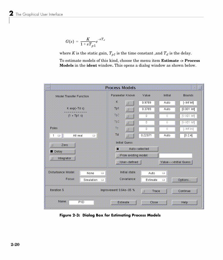
2 The Graphical User Interface
2-20
where K is the static gain, Tp1 is the time constant ,and Td is the delay.
To estimate models of this kind, choose the menu item Estimate -> Process Models in the ident window. This opens a dialog window as shown below.
Figure 2-3: Dialog Box for Estimating Process Models
G s( ) K1 sTp1+----------------------e
sTd–=
Estimating Models
2-21
In this dialog you enter how many time constants (poles) to estimate and whether to include a time-delay term and an extra zero in the numerator of the transfer function. You can also enforce an integration for self-regulating processes. Moreover, there is a choice to force all time constants to be real or to allow underdamped modes (complex poles).
The dialog can handle an arbitrary amount of inputs, but only one output signal.
Some Further Estimation OptionsThe dialog box also has four menus that offer further options.
Disturbance Model allows you to include a first- or second-order model for the additive disturbances to the output.
Focus allows you to choose between a frequency weighting that concentrates on the model’s prediction or simulation performance. Another alternative is prefiltering, which was described in “Prefiltering” on page 2-13.
Moreover, the menu InitialState gives options to estimate the initial state or to fix it to zero. The value Auto makes an automatic choice among these options.
Finally, the menu Covariance allows the choice between Estimate and None. The normal situation is that the covariance of the model is estimated, so that various uncertainty measures can be displayed in the plots.
Initial Parameter Values and Parameter BoundsIf no prior knowledge is available about the parameters, a startup routine is invoked to come up with initial parameter estimates. These are further iterated upon to give the best possible model fit to the data. The text AUTO is used to indicate that no initial guess is provided and an automatic process is invoked to estimate the initial values. If no qualified guess is available, this is usually a better alternative than entering an ad hoc value. However, if the estimation process gives parameter values that seem unreasonable, it might be worthwhile to try out various initial guesses and upper and/or lower limits of the parameters. Note that if you estimate a time delay, you must always provide un upper limit for the delay in order to secure efficient algorithms. The default value of this upper bound is 30 sampling intervals.
2 The Graphical User Interface
2-22
Iteration InformationThe dialog window also gives online information about the progress of the iterative optimization of the fit between data and model. The iteration number, the fit at the current information, as well as the improvement in fit (in percent) compared to the previous iteration, are shown. There is also a possibility to abort the iterations and save the current model, after the current iteration is finished. You access parameters that affect the minimization process by clicking Options.
Estimation of Parametric Models The System Identification Toolbox supports a wide range of model structures for linear systems. Except for process models, they are all accessed by the menu item Estimate -> Parametric Models in the ident window. This opens a dialog box Parametric Models, which contains the basic dialog for all parametric estimation as shown below.
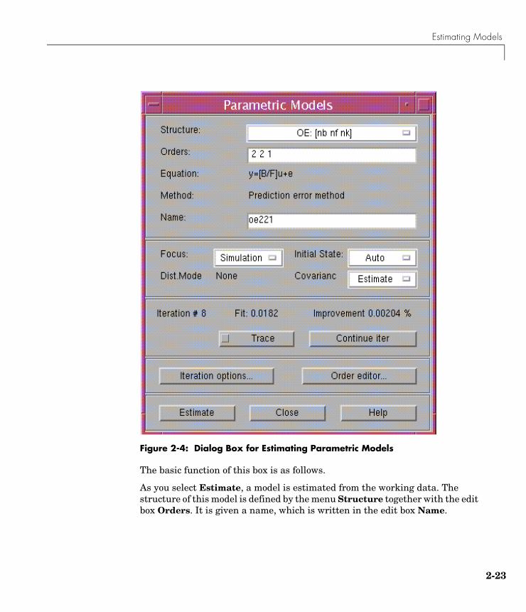
Estimating Models
2-23
Figure 2-4: Dialog Box for Estimating Parametric Models
The basic function of this box is as follows.
As you select Estimate, a model is estimated from the working data. The structure of this model is defined by the menu Structure together with the edit box Orders. It is given a name, which is written in the edit box Name.
2 The Graphical User Interface
2-24
The GUI will always suggest a default model name in the Name box, but you can change it to any string before clicking Estimate. (If you intend to export the model later, avoid spaces in the name.)
The interpretation of the model structure information (typically integers) in the Order box depends on the selected structure in the menu. This covers, typically, six choices:
• ARX models
• ARMAX model
• Output-error (OE) models
• Box-Jenkins (BJ) models
• State-space models
• Model structure defined by initial model (user-defined structures)
You can fill out the Order box yourself at any time, but for assistance you can select Order Editor. This opens another dialog box, depending on the chosen structure, in which the desired model order and structure information can be entered in a simpler fashion.
You can also enter the name of a MATLAB workspace variable in the Order edit box. This variable should then have a value that is consistent with the necessary orders for the chosen structure.
Note For the state-space structure and the ARX structure, you can enter several orders and combinations of orders. Then all corresponding models will be compared and displayed in a special dialog window for you to select suitable ones. This could be a useful tool to select good model orders. This option is described in more detail later in this section. When it is available, a button Order selection is visible.
Estimation Method A common and general method of estimating the parameters is the prediction error approach, where simply the parameters of the model are chosen so that the difference between the model’s (predicted) output and the measured output is minimized. This method is available for all model structures. Except for the ARX case, the estimation involves an iterative numerical search for the best fit.
Estimating Models
2-25
Some information from this search is given online in the dialog box. By clicking Iteration options, you get access to a number of options that govern the search process. (See “Algorithm Properties” on page 4-14.)
For some model structures (the ARX model, and black-box state-space models) methods based on correlation are also available — Instrumental Variable (IV) and Subspace (N4SID) methods. The choice between methods is made in the Parametric Models dialog box.
The dialog box also has three menus that offer further options. Focus allows you to choose between a frequency weighting that concentrates on the model’s prediction or simulation performance. Another alternative is prefiltering, which was described in “Prefiltering” on page 2-13. Moreover, the menu InitialState gives options to estimate the initial state or to fix it to zero. The value Auto makes an automatic choice among these options. Finally, the menu Covariance allows the choice between Estimate and None. The normal situation is that the covariance of the model is estimated, so that various uncertainty measures can be displayed in the plots. However, for high-order state-space models estimated by N4SID, or large multivariable ARX models, the computation of the covariance matrix can take quite a long time. Choosing Covariance: None will then greatly reduce the computation time.
Resulting Models The estimated model is inserted into the GUI’s model board. You can then examine its various properties and compare them with other models’ properties using the Model View plots. More about that in “Examining Models” on page 2-33.
To take a look at the model itself, double-click the model’s icon (or right-click or Ctrl+click). The Data/Model Info window that opens gives you information about how the model was estimated. You can also select the Present button, which will list the model and its parameters with estimated standard deviations in the MATLAB Command Window.
If you need to work further with the model, you can export it by dragging and dropping it over the To Workspace icon, and then apply any MATLAB and toolbox commands to it. (See, in particular, the commands ssdata, tfdata, d2c, and get in Chapter 4, “Function Reference.”)
2 The Graphical User Interface
2-26
How to Know Which Structure and Method to Use There is no simple way to find out “the best model structure”; in fact, for real data, there is no such thing as a best structure. Some routes to find good and acceptable models are described in “A Startup Identification Procedure” on page 1-14. It is best to be generous at this point. It often takes just a few seconds to estimate a model, and by the different validation tools described in the next section, you can quickly find out if the new model is any better than the ones you had before. There is often a significant amount of work behind the data collection, and spending a few extra minutes trying out several different structures is usually worthwhile.
ARX Models
The Structure The most used model structure is the simple linear difference equation
which relates the current output y(t) to a finite number of past outputs y(t-k) and inputs u(t-k).
The structure is thus entirely defined by the three integers na, nb, and nk. na is equal to the number of poles and nb 1 is the number of zeros, while nk is the pure time delay (the dead time) in the system. For a system under sampled-data control, typically nk is equal to 1 if there is no dead time.
For multiinput systems, nb and nk are row vectors, where the ith element gives the order/delay associated with the ith input.
Entering the Order Parameters The orders na, nb, and nk can either be directly entered into the edit box Orders in the Parametric Models window, or selected using the menus in the Order Editor.
Estimating Many Models Simultaneously By entering any or all of the structure parameters as vectors, using the MATLAB colon notation, such as na=1:10, you define many different structures that correspond to all combinations of orders. When you select
y t( ) a1y t 1–( ) … anay t na–( ) =+ + +
b1u t nk–( ) … bnbu t nk– nb– 1+( )+ +

Estimating Models
2-27
Estimate, models corresponding to all of these structures are computed. A special plot window then opens that shows the fit of these models to validation data. By clicking in this plot, you can enter any models of your choice into the model board.
Multiinput models: For multiinput models you can enter each of the input orders and delays as a vector. The number of models resulting from all combinations of orders and delays can, however, be very large. As an alternative, you can enter one vector (such as nb=1:10) for all inputs and one vector for all delays. Then only models that have the same orders and delays from all inputs are computed.
Estimation MethodsThere are two methods to estimate the coefficients a and b in the ARX model structure:
Least Squares: Minimizes the sum of squares of the right side minus the left side of the expression above, with respect to a and b. This is obtained by selecting ARX in the Method box.
Instrumental Variables: Determines a and b so that the error between the right and left sides becomes uncorrelated with certain linear combinations of the inputs. This is obtained by selecting IV in the Method box.
The methods are described in more detail in the reference pages for arx and iv4.
Multioutput Models For a multioutput ARX structure with ny outputs and nu inputs, the difference equation above is still valid. The only change is that the coefficients a are ny-by-ny matrices and the coefficients b are ny-by-nu matrices.
The orders [NA NB NK] define the model structure as follows:
NA: an ny-by-ny matrix whose i-j entry is the order of the polynomial (in the delay operator) that relates the jth output to the ith output
NB: an ny-by-nu matrix whose i-j entry is the order of the polynomial that relates the jth input to the ith output
NK: an ny-by-nu matrix whose i-j entry is the delay from the jth input to the ith output
2 The Graphical User Interface
2-28
The Order Editor dialog box allows the choices
NA = na∗ ones(ny,ny)NB = nb∗ ones(ny,nu)NK = nk∗ ones(ny,nu)
where na, nb, and nk are chosen by the menus.
For custom order choices, construct a matrix [NA NB NK] in the MATLAB Command Window and enter the name of this matrix in the Order edit box in the Parametric Models window.
Note that the possibility to estimate many models simultaneously is not available for multioutput ARX models.
See “Defining Model Structures” on page 3-39 for more information on multioutput ARX models.
ARMAX, Output-Error (OE), and Box-Jenkins (BJ) ModelsThere are several elaborations of the basic ARX model, where different disturbance models are introduced. These include well-known model types, such as ARMAX, Output-Error (OE), and Box-Jenkins (BJ).
The General StructureA general input-output linear model for a single-output system with input u and output y can be written
Here ui denotes input #i, and A, Bi, C, D, and Fi, are polynomials in the shift operator (z or q). (Don’t be intimidated by this: It is just a compact way of writing difference equations; see below.)
The general structure is defined by giving the time-delays nk and the orders of these polynomials (i.e., the number of poles and zeros of the dynamic model from u to y, as well as of the disturbance model from e to y).
A q( )y t( ) Bi q( ) Fi q( ) ]⁄ ui t nki–( ) C q( ) D q( ) ]⁄ e t( )[+[
i 1=
nu
∑=
Estimating Models
2-29
The Special Cases Most often the choices are confined to one of the following special cases.
ARX:
ARMAX:
OE: (Output-Error)
BJ: (Box-Jenkins)
The “shift operator polynomials” are just compact ways of writing difference equations. For example, the ARMAX model in longhand would be
Note that A(q) corresponds to poles that are common between the dynamic model and the disturbance model (useful if disturbances enter the system “close to” the input). Likewise determines the poles that are unique for the dynamics from input # i, and D(q) the poles that are unique for the disturbances.
The reason for introducing all these model variants is to provide for flexibility in the disturbance description and to allow for common or different poles (dynamics) for the different inputs.
Entering the Model Structure Use the Structure menu in the Parametric Models dialog to choose between the ARX, ARMAX, Output-Error, and Box-Jenkins structures. Note that if the working data set has several outputs, only the first choice is available. For time series (data with no input signal) only AR and ARMA are available among these choices. These are the time series counterparts of ARX and ARMAX.
The orders of the polynomials are selected by the menus in the Order Editor dialog window, or by directly entering them in the edit box Orders in the Parametric Models window. When the order editor is open, the default orders, entered as you change the model structure, are based on previously used orders.
A q( )y t( ) B q( )u t nk–( ) e t( )+=
A q( )y t( ) B q( )u t nk–( ) C q( )e t( )+=
y t( ) B q( ) F q( )⁄[ ] u t nk–( ) e t( )+=
y t( ) B q( ) F q( )⁄[ ] u t nk–( ) C q( ) D q( )⁄[ ] e t( )+=
y t( ) a1y t 1–( ) … anay t na–( )+ + + b1u t nk–( ) …+ +=
bnbu t nk– nb– 1+( ) e t( ) c1e t 1–( ) … cnce t nc–( )+ + + +
Fi q( )
2 The Graphical User Interface
2-30
Estimation Method The coefficients of the polynomials are estimated using a prediction error/maximum likelihood method, by minimizing the size of the error term “e” in the expression above. Several options govern the minimization procedure. These are accessed by activating Iteration Control in the Parametric Models window and selecting Options.
The algorithms are further described in Chapter 4, “Function Reference,” under armax, Algorithm Properties, bj, oe, and pem. See also “Parametric Model Estimation” on page 3-28 and “Defining Model Structures” on page 3-39.
Note These model structures are available only for the scalar output case. For multioutput models, the state-space structures offer the same flexibility. Also note that it is not possible to estimate many different structures simultaneously for the input-output models.
State-Space Models
The Model Structure The basic state-space model in innovations form can be written
x(t+1) = A x(t) + B u(t) + K e(t)
y(t) = C x(t) + D u(t) + e(t)
The System Identification Toolbox supports two kinds of parameterizations of state-space models: black-box, free parameterizations, and parameterizations custom-made for the application. The latter are discussed in “User-Defined Model Structures” on page 2-32. First we will discuss the black-box case.
Entering Black-Box State-Space Model Structures The most important structure index is the model order; i.e., the dimension of the state vector x.
Use the menu in the Order Editor to choose the model order, or enter it directly into the Orders edit box in the Parametric Models window. You can further affect the chosen model structure:
Estimating Models
2-31
• Fixing K to zero gives an Output-Error method; i.e., the difference between the model’s simulated output and the measured one is minimized. Formally, this corresponds to an assumption that the output disturbance is white noise. This is done by the menu under Disturbance Model.
• The delays from the input can be chosen independently for each input. It will be a row vector nk, with nu entries. When the delay is larger than or equal to one, the D-matrix in the discrete time model is fixed to zero. For physical systems without a pure time delay that are driven by piecewise constant inputs, nk = 1 is a natural assumption. This is also the default. The delays nk can be set either in the order editor or directly in the Orders box as numbers in square brackets.
• The initial state X0 can either be estimated, set to zero, or “backcast.” This is handled by the menu Initial State.
Estimating Many Models Simultaneously By entering a vector for the model order, using the MATLAB colon notation, (such as 1:10) all indicated orders will be computed using a preliminary method. You can then enter models of different orders into the model board by clicking in a special graph that contains information about the models.
Estimation Methods There are two basic methods for the estimation.
PEM: Standard prediction error/maximum likelihood method, based on iterative minimization of a criterion. The iterations are started up at parameter values that are computed from n4sid. The parameterization of the matrices A, B, C, D, and K is free. The search for minimum is controlled by a number of options. These are accessed from the Option button in the Iteration Control window.
N4SID: Subspace-based method that does not use iterative search. The quality of the resulting estimates may significantly depend on some options called N4Weight and N4Horizon. These options can be chosen in the Order Editor dialog. If N4Horizon is entered with several rows, the models corresponding to the horizons in each row are examined separately using the working data. The best model in terms of prediction (or simulation, if K = 0) performance is selected. A figure is shown that illustrates the fit as a function of the horizon. If the N4Horizon box is left empty, a default choice is made.
See the reference pages for n4sid and pem for more information.
2 The Graphical User Interface
2-32
User-Defined Model Structures
State-Space Structures The System Identification Toolbox supports user-defined linear state-space models of arbitrary structure. Using the idss model structure, known and unknown parameters in the A, B, C, D, K, and X0 matrices can be easily defined both for discrete- and continuous-time models. The idgrey object allows you to use a completely arbitrary graybox structure, defined by an M-file. The model object properties can be easily manipulated. See the reference pages for idss and idgrey and “Structured State-Space Models with Free Parameters: the idss Model” on page 3-48.
To use these structures in conjunction with the GUI, just define the appropriate structure in the MATLAB Command Window. Then use the Structure menu to select By Initial Model, enter the variable name of the structure in the edit box Initial Model in the Parametric Models window, and select Estimate.
Any Model Structure Arbitrary model structures can be defined using the System Identification Toolbox model objects:
• idpoly: Creates input-output structures for single-output models
• idss: Creates linear state-space models with arbitrary free parameters
• idgrey: Creates completely arbitrary parameterizations of linear systems
• idarx: Creates multivariable ARX structures
In addition, all estimation commands create model structures in terms of the resulting models.
Enter the name of any model structure in the box Orders (or Initial model) in the window Parametric Models and then select Estimate. Then the parameters of the model structure are adjusted to the chosen working data set. The method is a standard prediction error/maximum likelihood approach that iteratively searches for the minimum of a criterion. Options that govern this search are accessed by the Option button in the Iteration Control window.
The name of the initial model must be a variable either in the workspace or in the model board. In the latter case you can just drag and drop it over the Orders/Initial model box.
Examining Models
2-33
Examining ModelsEstimating a model is just a first step. It must now be examined, compared with other models, and tested with new data sets. You do this primarily using the six Model View functions at the bottom of the main ident window:
• Frequency response
• Transient response
• Poles and zeros
• Noise spectrum
• Model output
• Model residuals
In addition, you can double-click the model’s icon to get Text Information about the model. Finally, you can export the model to the MATLAB workspace and use any commands for further analysis and model use.
Views and Models The basic idea is that if a certain View window is open (selected), then all models in the Model Summary Board that are selected will be represented in the window. The curves in the View window can be clicked in and out by selecting and clearing the models in an online fashion. You select and clear a model by clicking its icon. A selected model is marked with a thicker line in its icon.
On color screens, the curves are color coded along with the model icons in the model board. Before printing a plot it might be a good idea to separate the line styles (menu item under Style). This could also be helpful on black and white screens.
Note that models that are obtained by spectral analysis only can be represented as frequency response and noise spectra, and that models estimated by correlation analysis only can be represented as transient response.
The Plot Windows The six views all give similar plot windows, with several common features. They have a common menu bar, which covers some basic functions.
2 The Graphical User Interface
2-34
First of all, note that there is a zoom function in the plot window. By dragging with the left mouse button down, you can draw rectangles, which are enlarged when the mouse button is released. Double-clicking restores the original axis scales. For plots with two axes, the x-axes scales are locked to each other. A single click on the left mouse button zooms in by a factor of two, while the middle button zooms out. The zoom function can be deactivated if desired. Just select the menu item Zoom under Style.
Second, pointing to any curve in the plot and pressing the right mouse button identifies the curve with model name and present coordinates.
The common menu bar covers the following functions.
FileFile allows you to copy the current figure to another standard MATLAB figure window. This might be useful, for example, when you intend to print a customized plot. Other File items cover printing the current plot and closing the plot window.
OptionsOptions first of all covers actions for setting the axes scaling. This menu item also gives a number of choices that are specific for the plot window in question, such as a choice between step response or impulse response in the Transient response window.
An important option is the possibility of showing confidence intervals. Each estimated model property has some uncertainty. This uncertainty can be estimated from data. By selecting Show confidence intervals, a confidence region around the nominal curve (model property) will be marked (by dash-dotted lines). The level of confidence can also be set under this menu item.
Note Confidence intervals are supported for most models and properties, except models estimated using etfe, and the k-step ahead prediction property. For n4sid, the covariance properties are actually not fully known. The Cramer-Rao lower limit for the covariance matrix is then used instead.

Examining Models
2-35
StyleThe Style menu gives access to various ways of affecting the plot. You can add gridlines, turn the zoom on and off, and change the line styles. The menu also covers a number of other options, like choice of units and scale for the axis.
ChannelFor multivariate systems, you can choose which input-output channel to examine. The current choice is marked in the figure title.
HelpThe Help menu has a number of items, which explain the plot and its options.
Frequency Response and Disturbance Spectra All linear models that are estimated can be written in the form
y(t)=G(z)u(t)+v(t)
where G(z) is the (discrete-time) transfer function of the system and v(t) is an additive disturbance. The frequency response or frequency function of the
system is the complex-valued function viewed as a function of angular frequency ω.
This function is often graphed as a Bode diagram, i.e., the logarithm of the
amplitude (the absolute value) of as well as the phase (the argument)
of are plotted against the logarithm of frequency ω in two separate plots. These plots are obtained by selecting the Model View Frequency Response in the main ident window.
The estimated spectrum of the disturbance v is plotted as a power spectrum by choosing the Model View Noise Spectrum.
If the data is a time series y (with no input u), then the spectrum of y is plotted under Noise Spectrum, and no frequency functions are given.
Transient ResponseInsight into a model’s dynamic properties is obtained by looking at its step response or impulse response. This is the output of the model when the input
G eiωT( )
G eiωT( )
G eiωT( )
2 The Graphical User Interface
2-36
is a step or an impulse. These responses are plotted when the Model View Transient Response is selected.
It is informative to compare the transient response of a parametric model with the one that was estimated using correlation analysis. If there is good agreement between the two, you can be confident that some correct features have been picked up. It is useful to check the confidence intervals around the responses to see what “good agreement” could mean quantitatively.
Many models provide a description of the additive disturbance v(t).
v(t)=H(z)e(t)
Here H(z) is a transfer function that describes how the disturbance v(t) can be thought of as generated by sending white noise e(t) through it. To display the properties of H, you can choose channels (in the Channel menu) that have noise components as inputs. The names of these channels are like e@ynam, for the noise component that directly affects the output with name ynam.
Poles and ZerosThe poles of a system are the roots of the denominator of the transfer function G(z), while the zeros are the roots of the numerator. In particular the poles have a direct influence on the dynamic properties of the system.
The poles and zeros of G (and H ) are plotted by choosing the Model View Poles and Zeros.
It is useful to turn on the confidence intervals in this case. They will reveal which poles and zeros could cancel each other (their confidence regions overlap). That is an indication that a lower-order dynamic model could be used.
For multivariable systems, it is the poles and zeros of the individual input/output channels that are displayed. To obtain the so-called transmission zeros, you will have to export the model and then apply the command tzero. (This requires the Control System Toolbox.)
Compare Measured and Model Outputs A good way of obtaining insight into the quality of a model is to simulate the model with the input from a fresh data set and compare the simulated output with the measured one. This gives a good feel for which properties of the system have been picked up by the model, and which have not.
Examining Models
2-37
This test is obtained by selecting the Model View Model Output. Then the data set currently in the Validation Data box will be used for the comparison. The fit will also be displayed. This is computed as the percentage of the output variation that is reproduced by the model. So, a model that has a fit of 0% gives the same mean square error as just setting the model output to be the mean of the measured output.
If the model is unstable, or has integration or very slow time constants, the levels of the simulated and the measured output may drift apart, even for a model that is quite good (at least for control purposes). It is then a good idea to evaluate the model’s predicted output rather than the simulated one. With a prediction horizon of k, the k-step ahead predicted output is then obtained as follows:
The predicted value y(t) is computed from all available inputs (used according to the model) and all available outputs up to time t-k, . The simulation case, where no past outputs at all are used, thus formally corresponds to k=∞. To check whether the model has picked up interesting dynamic properties, it is wise to let the predicted time horizon (kT, T being the sampling interval) be larger than the important time constants.
Note here that different models use the information in past output data in their predictors in different ways. This depends on the disturbance model. For example, so called Output-Error models (obtained by fixing K to zero for state-space models and setting na=nc=nd=0 for polynomial models) do not use past outputs at all. The simulated and the predicted outputs, for any value of k, thus coincide.
The character of the comparison depends of the type of validation data. For frequency-domain input/output validation data, the amplitudes of the measured output signal are shown together with the models’ simulated output frequency response (which is the product of the input frequency domain signal and the model frequency response.) In this case, the predictions are not applicable. For frequency-response data the amplitude of the frequency response data is compared to the models’ frequency responses. Note that even though just the amplitudes are shown in the plots, the figure of fit refers to the distance between the functions as complex variables.
Residual Analysis In a model
u s( ) s t≤( )y s( ) s t k–≤( )
2 The Graphical User Interface
2-38
the noise source e(t) represents that part of the output that the model could not reproduce. It gives the “left-overs” or, in Latin, the residuals. For a good model, the residuals should be independent of the input. Otherwise, there would be more in the output that originates from the input and that the model has not picked up.
To test this independence, the cross-correlation function between input and residuals is computed by selecting the Model View Model Residuals. It is wise to also display the confidence region for this function. For an ideal model the correlation function should lie entirely between the confidence lines for positive lags. If, for example, there is a peak outside the confidence region for lag k, this means that there is something in the output y(t) that originates from u(t-k) and that has not been properly described by the model. The test is carried out using the validation data. If these were not used to estimate the model, the test is quite tough. See also “Model Structure Selection and Validation” on page 3-70.
For a model also to give a correct description of the disturbance properties (i.e., the transfer function H), the residuals should be mutually independent. This test is also carried out by the view Model Residuals, by displaying the autocorrelation function of the residuals (excluding lag zero, for which this function by definition is 1). For an ideal model, the correlation function should be entirely inside the confidence region.
For frequency-domain validation data the power spectrum of the residuals is shown, as well as the amplitude of the estimated transfer function from input(s) to residuals.
Text InformationBy double-clicking (right mouse button or Ctrl+click) the model icon, a Data/Model Info dialog box opens, which contains some basic information about the model. It also gives a diary of how the model was created, along with the notes that originally were associated with the estimation data set. At this point you can do a number of things.
PresentClicking the Present button displays details of the model in the MATLAB Command Window. The model’s parameters along with estimated standard deviations are displayed, as well as some other notes.
y t( ) G z( )u t( ) H z( )e t( )+=

Examining Models
2-39
ModifyYou can simply type in any text you want anywhere in the Diary and Notes field of the dialog box. You can also change the name of the model just by editing the text field with the model name. The color, which the model is associated with in all plots, can also be edited. Enter RGB values or a color name (such as 'y') in the corresponding box.
LTI ViewerIf you have the Control System Toolbox, you will see an icon To LTI Viewer in the main window. Dragging and dropping a model onto this icon opens the LTI Viewer. This viewer handles an arbitrary amount of models, but it requires all of them to have the same number of inputs and outputs. Note the the LTI viewer is not fully live when clicking in and out the models on the model board. Instead, the LTI viewer has its own interface for dealing with models and channel (right-click in the plot).
Further Analysis in the MATLAB WorkspaceAny model and data object can be exported to the MATLAB workspace by dragging and dropping its icon over the To Workspace box in the ident window.
Once you have exported the model to the workspace, there are many commands by which you can further transform it, examine it, and convert it to other formats for use in other toolboxes. Some examples of such commands are as follows:
Note that the commands ss, tf, and zkp transform the model to the Control System Toolbox’s LTI models. Moreover, if you have that toolbox, many of its LTI commands can be applied directly to the model objects of the Identification
d2c Transform to continuous time
ss, idss, ssdata Convert to state-space representation
tf, tfdata Convert to transfer function form
zpk, zpkdata Convert to zeros and poles

2 The Graphical User Interface
2-40
Toolbox. See “Connections Between the Control System Toolbox and the System Identification Toolbox” on page 3-95.
Also, if you need to prepare specialized plots that are not covered by the Views, all the System Identification Toolbox commands for computing and extracting simulations, frequency functions, zeros and poles, etc., are available. See Chapter 3, “Tutorial,” and Chapter 4, “Function Reference.”

Some Further GUI Topics
2-41
Some Further GUI TopicsThis section discusses a number of different topics.
Mouse Buttons and HotkeysThe GUI uses three mouse buttons. If you have fewer buttons on your mouse, the actions associated with the middle and right mouse buttons are obtained by Shift+click, Alt+click, or Ctrl+click, depending on the computer.
The Main ident WindowIn the main ident window the mouse buttons are used to drag and drop, to select/clear models and data sets, and to double-click to get text information about the object. You can use the left mouse button for all of this. A certain speedup is obtained if you use the left button for dragging and dropping, the middle one for selecting models and data sets, and the right one for double-clicking (actually for the right button, a single click is sufficient). On a slow machine a double-click from the left button might not be recognized.
The ident window also has a number of hot keys. By pressing a keyboard letter when it is the current window, you can quickly activate some functions. These are
• s: Computes the Spectral Analysis Model using the current options settings. (These can be changed in the dialog window that opens when you choose Spectral Model in the Estimate menu.)
• c: Computes Correlation Analysis Model using the current options settings.
• q: Computes the models associated with the Quickstart.
• d: Opens a dialog window for importing data objects.
Plot WindowsIn the various plot windows the action of the mouse buttons depends on whether zoom is activated or not.
Zoom Active: The left and middle mouse buttons are associated with the zoom functions as in the standard MATLAB zoom. The left button zooms in and the middle one zooms out. In addition, you can draw rectangles with the left button
2 The Graphical User Interface
2-42
to define the area to be zoomed. Double-clicking restores the original plot. The right mouse button is associated with special GUI actions that depend on the window. In the View plots, the right mouse button is used to identify the curves. Point and click a curve, and a box displays the name of the model/data set that the curve is associated with, and also the current coordinate values for the curve. In the Model Selection plots, the right mouse button is used to inspect and select the various models. In the Prefilter and Data Range plots, rectangles are drawn with this mouse button down, to define the selected range.
Zoom not active: The special GUI functions just mentioned are obtained by any mouse button.
The zoom is activated and deactivated under the menu item Style. The default setting differs between the plots.
Note Don’t activate the zoom from the command line! That will destroy the special GUI functions. (If you happen to do so anyway, quit the window and open it again.)
Troubleshooting in PlotsThe function Auto-range, which is found under the menu item Options, sets automatic scales to the plots. It is also a good function to invoke when you think that you have lost control over the curves in the plot. (This might happen, for example, if you zoom in a portion of a plot and then change the data of the plot.)
If the view plots don’t respond the way you expect them to, you can always quit the window and open it again. By quit here we mean using the underlying window system’s own quitting mechanism, which is called different things in the different platforms. The normal way to close a window is to use the Close function under the menu item File or to clear the corresponding check box.
Layout Questions and idprefs.matThe GUI comes with a number of preset defaults. These include the window sizes and positions, the colors of the different models, and the default options in the different View windows.

Some Further GUI Topics
2-43
The window sizes and positions, as well as the options in the plot windows, can be changed during the session in the standard way. If you want the GUI to start with your current window layout and current plot options, select menu item Options -> Save preferences in the main ident window. This saves the information in a file idprefs.mat. This file also stores information about the four most recent sessions with ident. This allows the session File menu to be correctly initialized. The session information is automatically stored upon exit. The layout and preference information is only saved when the indicated option is selected.
The file idprefs.mat is created the first time you close the GUI. It is stored in the same directory as your startup.m file by default. If this default does not work, you are prompted for a directory to store the file. This can be ignored, but then session and preference information cannot be saved.
To change or select a directory for idprefs.mat, use the command midprefs. See the midprefs reference page for details.
To change model colors and default options to your own customized choice, make a copy of the M-file idlayout.m to your own directory (which should be before the basic ident directory in the MATLABPATH), and edit it according to its instructions.
Customized PlotsIf you need to prepare hardcopies of your plots with specialized texts, titles, and so on, make a copy of the figure first, using Copy Figure under the File menu item. This produces a copy of the current figure in a standard MATLAB figure format.
For plots that are not covered by the View windows, (e.g., Nyquist plots), you have to export the model to the MATLAB workspace and construct the plots there.
What Cannot Be Done Using the GUIThe GUI covers primarily everything you would like to do to examine data, estimate models, and evaluate and compare models. It does not cover
• Generation (simulation) of data sets
• Model creation (other than by estimation)
• Model manipulation and conversion
2 The Graphical User Interface
2-44
• Recursive (online) estimation algorithms
To see what M-files are available in the toolbox for these functions, see “The Toolbox Commands” on page 3-3, as well as “Simulation and Prediction” on page 4-3, “Model Structure Creation” on page 4-5, “Manipulating Model Structures” on page 4-6, “Model Conversions” on page 4-6, and “Recursive Parameter Estimation” on page 4-8.
Note that at any point you can export a data set or a model to the MATLAB workspace (by dragging and dropping its icon on the To Workspace icon). There you can modify and manipulate it any way you want and then import it back into ident. You can, for example, construct a continuous-time model from an estimated discrete-time one (using d2c), and then use the model views to compare the two.
3
Tutorial
Overview (p. 3-2) A quick look at the contents of this tutorial
The Toolbox Commands (p. 3-3) An overview of the organization of system identification commands
An Introductory Example to Command Mode (p. 3-5)
An worked out example that uses the command line only.
The System Identification Problem (p. 3-9)
A discussion of the basic issues in system identification
Data Representation and Nonparametric Model Estimation (p. 3-19)
Various ways to represent data
Parametric Model Estimation (p. 3-28) Estimating models using parametric methods
Defining Model Structures (p. 3-39) An overview of available model structures
Examining Models (p. 3-57) How to plot the responses and further examine estimated models
Model Structure Selection and Validation (p. 3-70)
A discussion of the process used to select model structure, and how to validate an identified model
Dealing with Data (p. 3-81) A collection of topics about data preprocessing, such as detrending and filtering
Recursive Parameter Estimation (p. 3-85) An overview of the algorithms used in recursive estimation
Some Special Topics (p. 3-92) Various topics, including time series modeling and connections between The System Identification Toolbox and The Control System Toolbox
3 Tutorial
3-2
OverviewThis chapter has three purposes:
• Gives an overview of system identification theory, the basic models and disturbance descriptions used, and the character of the basic algorithms. It also provides some practical advice for a number of issues that are essential for a successful application.
• Describes the commands and objects of the System Identification Toolbox, their syntax and use. If you primarily use the graphical user interface (GUI), you will not have to bother about these aspects.
• Describes the commands that are not reached from the GUI, that is, simulation, the recursive algorithms, and more advanced model structure definitions.
The Toolbox Commands
3-3
The Toolbox CommandsIt might be useful to recognize several layers of the System Identification Toolbox. Initially concentrate on the first layer of basic tools, which contains the commands from the System Identification Toolbox that any user must master. You can proceed to the next levels whenever an interest or the need from the applications warrants it. The layers are described in the following paragraphs:
Layer 0: Help Functions. Help ident gives an overview of available commands. idhelp gives access to a “micromanual” of command-line help, with several subhelps like idhelp evaluate, etc. There is also a command advice that can be applied to any data set and any model.
advice(data)advice(model)
This gives text information on the screen about the quality of the data/model and some advice on how to proceed.
Layer 1: Basic Tools for Estimating Black-Box Models. The first layer contains the basic tools for estimating models from measured data. It is necessary to know the basics of the data representation and the simple commands to build and evaluate black-box models. The commands are
• For data representation: iddata, plot
• For nonparametric estimation of impulse and frequency response: impulse, step, spa
• For estimating black-box models of state-space and input-output type: pem, arx
• For evaluating models: compare, resid
• For displaying model characteristics: bode, nyquist, pzmap, step, view
• Looking at parametric model characteristics: by field referencing, like Mod.A, Mod.dA, etc.
The corresponding background is given in the next few sections of this tutorial.
Layer 2: Creating Models for Simulation and Transforming Models. To define models, to generate inputs, and to simulate models

3 Tutorial
3-4
idarx, idpoly, idproc, idss, idinput, sim
To transform models to other representations
arxdata, polydata, ssdata, tfdata, zpkdata
Layer 3: Model Structure Selection. The third layer of the toolbox contains some useful techniques to select orders and delays.
arxstruc, selstruc
Layer 4: Structured Models and Further Model Conversions. The fourth layer contains transformations between continuous and discrete time, and functions for estimating completely general model structures for linear systems. The commands are
c2d, d2c, idss, idgrey, pe, predictss, tf, zp, frd (to be used with the Control System Toolbox)
The corresponding material is covered in “Defining Model Structures” on page 3-39 and in “Examining Models” on page 3-57.
Layer 5: Recursive Identification. Recursive (adaptive, online) methods of parameter estimation are covered by the commands
rarmax, rarx, rbj, roe, rpem, rplr
They are covered in “Recursive Parameter Estimation” on page 3-85.
See Chapter 4, “Function Reference,” for a complete list of available functions.
An Introductory Example to Command Mode
3-5
An Introductory Example to Command ModeA demonstration M-file called iddemo.m provides several examples of what might be typical sessions with the System Identification Toolbox. To start the demo, execute iddemo from inside MATLAB.
Before giving a formal treatment of the capabilities and possibilities of the toolbox, this example is designed to get you started with the software quickly. This example is essentially the same as demo #2 in iddemo. You might want to invoke MATLAB at this time, execute the demo, and follow along.
Example DetailsData has been collected from a laboratory scale process. (Feedback’s Process Trainer PT326; see page 526 in Ljung (1999). For more references, see “Reading More About System Identification” on page 1-21.) The process operates much like a common hand-held hair dryer. Air is blown through a tube after being heated at the inlet to the tube. The input to the process is the power applied to a mesh of resistor wires that constitutes the heating device. The output of the process is the air temperature at the outlet, measured in volts by a thermocouple sensor.
One thousand input-output data points were collected from the process as the input was changed in a random fashion between two levels. The sampling interval is 80 ms. The data was loaded into MATLAB in ASCII form and is now stored as the vectors y2 (output) and u2 (input) in the file dryer2.mat.
First load the data.
load dryer2
It contains the input vector u2, the output vector y2. Now form the data object.
dry = iddata(y2,u2,0.08);
To get information about the data, just type the name.
dry
To get an overview of all the information contained in the iddata object dry, type
get(dry)
3 Tutorial
3-6
For better bookkeeping, give names to input and outputs.
dry.InputName = 'Power';
dry.OutputName = 'Temperature';
Select the 300 first values for building a model.
ze = dry(1:300);
Plot the interval from sample 200 to 300.
plot(ze(200:300)),
Remove the constant levels and make the data zero-mean.
ze = detrend(ze);
First estimate the impulse response of the system by correlation analysis to get some idea of time constants and the like.
impulse(ze,'sd',3)
This gives a plot with dash-dotted lines marking a confidence region corresponding to three standard deviations (ca 99.9%). From this it is easy to see if there is a time delay in the system.
Seeing a Time Delay ? The simplest way to get started is to build a state-space model where the order is automatically determined, using a prediction error method.
m1 = pem(ze)
When the calculations are finished, a display of the basic information about m1 is shown. Anytime m1 is typed, this display is shown. Typing present(m1) gives some more information about the model, including uncertainties.
To retrieve the properties of this model we could, for example, find the A matrix of the state space representation by
A = m1.a
m1 is a model object, and
get(m1)
gives a list of all information stored in the model.

An Introductory Example to Command Mode
3-7
m1.EstimationInfo or m1.es for short gives information about the estimation process, loss functions, etc.
How Good Is the ModelHow good is this model? One way to find out is to simulate it and compare the model output with measured output. We then select a portion of the original data that was not used to build the model, for example, from sample 800 to 900.
zv = dry(800:900);zv = detrend(zv);compare(zv,m1);
The Bode plot of the model is obtained by
bode(m1)
An alternative is to consider the Nyquist plot, and mark uncertainty regions at certain frequencies with ellipses, corresponding to three standard deviations.
nyquist(m1,'sd',3)
We can also compare the step response of the model with one that is directly computed from data (ze) in a nonparametric way.
step(m1,ze)
To study a model with prescribed structure, we compute a difference equation model with two poles, one zero, and three delays.
m2 = arx(ze,[2 2 3])
This gives a model of the form
where T is the sampling interval (here 0.08 second). This model, known as an ARX model, tries to explain or compute the value of the output at time t, given previous values of y and u. To compare its performance on validation data with m1, type
compare(zv,m1,m2);
Compare and PlotCompute and plot the poles and zeros of the models.
y t( ) a1y t T–( ) a2y t 2T–( )+ + b1u t 3T–( ) b2u t 4T–( )+=

3 Tutorial
3-8
pzmap(m1,m2)
The uncertainties of the poles and zeros can also be plotted.
pzmap(m1,m2,'sd',3), % '3' denotes the number of standard deviations
Estimate the frequency response by a nonparametric spectral analysis method.
gs = spa(ze);
Compare with the frequency functions from the parametric models.
bode(m1,m2,gs)
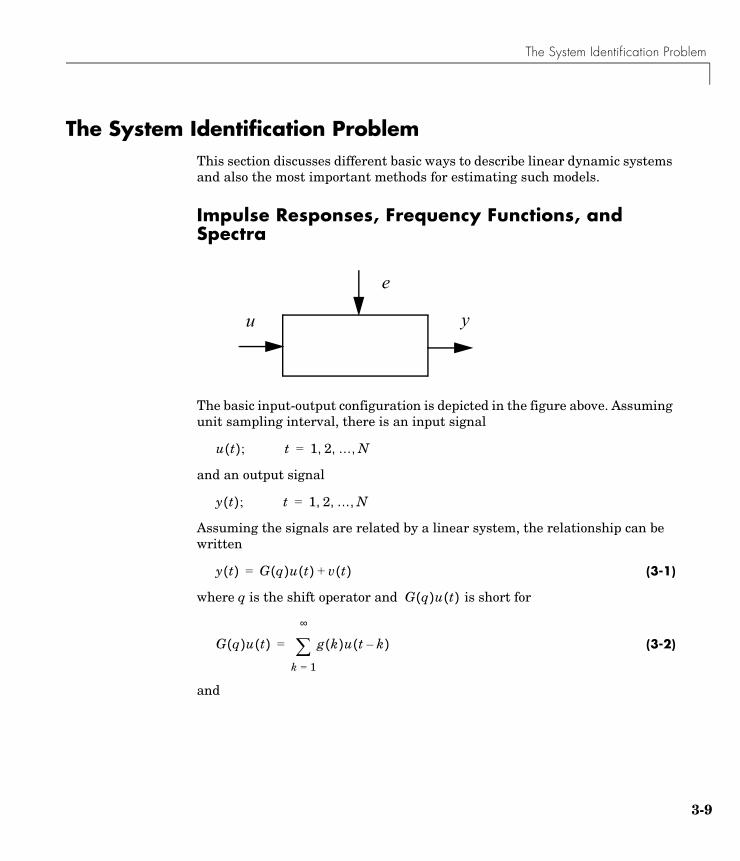
The System Identification Problem
3-9
The System Identification ProblemThis section discusses different basic ways to describe linear dynamic systems and also the most important methods for estimating such models.
Impulse Responses, Frequency Functions, and Spectra
The basic input-output configuration is depicted in the figure above. Assuming unit sampling interval, there is an input signal
and an output signal
Assuming the signals are related by a linear system, the relationship can be written
(3-1)
where q is the shift operator and is short for
(3-2)
and
y
e
u
u t( ); t 1 2 … N, , ,=
y t( ); t 1 2 … N, , ,=
y t( ) G q( )u t( ) v t( )+=
G q( )u t( )
G q( )u t( ) g k( )u t k–( )
k 1=
∞
∑=
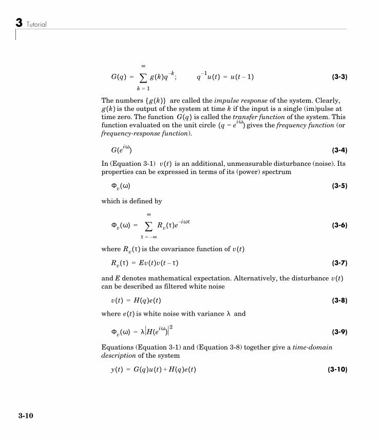
3 Tutorial
3-10
(3-3)
The numbers are called the impulse response of the system. Clearly, is the output of the system at time k if the input is a single (im)pulse at
time zero. The function is called the transfer function of the system. This function evaluated on the unit circle gives the frequency function (or frequency-response function).
(3-4)
In (Equation 3-1) is an additional, unmeasurable disturbance (noise). Its properties can be expressed in terms of its (power) spectrum
(3-5)
which is defined by
(3-6)
where is the covariance function of
(3-7)
and E denotes mathematical expectation. Alternatively, the disturbance can be described as filtered white noise
(3-8)
where is white noise with variance and
(3-9)
Equations (Equation 3-1) and (Equation 3-8) together give a time-domain description of the system
(3-10)
G q( ) g k( )q k– ;
k 1=
∞
∑= q 1– u t( ) u t 1–( )=
g k( ){ }g k( )
G q( )q eiω=( )
G eiω( )
v t( )
Φv ω( )
Φv ω( ) Rv τ( )e iωτ–
τ ∞–=
∞
∑=
Rv τ( ) v t( )
Rv τ( ) Ev t( )v t τ–( )=
v t( )
v t( ) H q( )e t( )=
e t( ) λ
Φv ω( ) λ H eiω( )2
=
y t( ) G q( )u t( ) H q( )e t( )+=
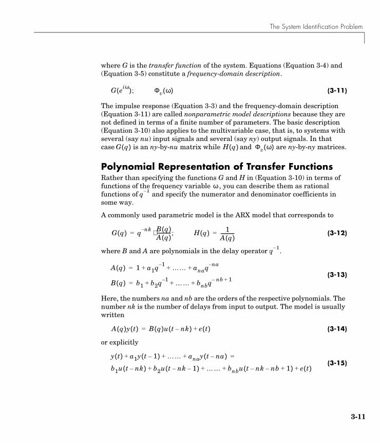
The System Identification Problem
3-11
where G is the transfer function of the system. Equations (Equation 3-4) and (Equation 3-5) constitute a frequency-domain description.
(3-11)
The impulse response (Equation 3-3) and the frequency-domain description (Equation 3-11) are called nonparametric model descriptions because they are not defined in terms of a finite number of parameters. The basic description (Equation 3-10) also applies to the multivariable case, that is, to systems with several (say nu) input signals and several (say ny) output signals. In that case is an ny-by-nu matrix while and are ny-by-ny matrices.
Polynomial Representation of Transfer FunctionsRather than specifying the functions G and H in (Equation 3-10) in terms of functions of the frequency variable , you can describe them as rational functions of and specify the numerator and denominator coefficients in some way.
A commonly used parametric model is the ARX model that corresponds to
(3-12)
where B and A are polynomials in the delay operator .
(3-13)
Here, the numbers na and nb are the orders of the respective polynomials. The number nk is the number of delays from input to output. The model is usually written
(3-14)
or explicitly
(3-15)
G eiω( ); Φv ω( )
G q( ) H q( ) Φv ω( )
ωq 1–
G q( ) q nk– B q( )A q( )------------;⋅= H q( ) 1
A q( )------------=
q 1–
A q( ) 1 a1q 1– …… anaq na–+ + +=
B q( ) b1 b2q 1– …… bnbq nb– 1++ + +=
A q( )y t( ) B q( )u t nk–( ) e t( )+=
y t( ) a1y t 1–( ) …… anay t na–( )+ + + =
b1u t nk–( ) b2u t nk– 1–( ) …… bnbu t nk– nb– 1+( ) e t( )+ + + +
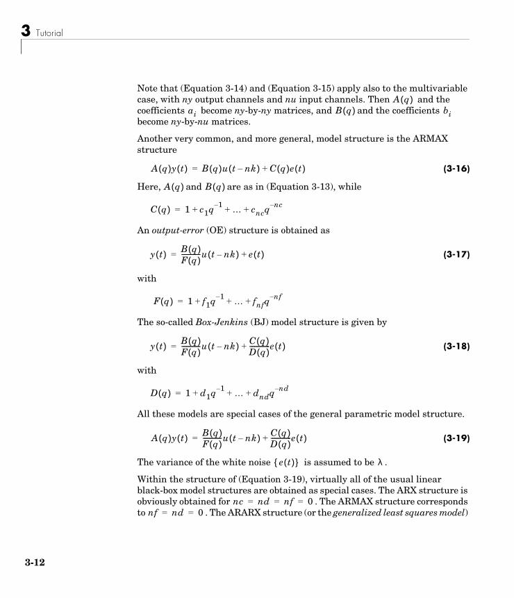
3 Tutorial
3-12
Note that (Equation 3-14) and (Equation 3-15) apply also to the multivariable case, with ny output channels and nu input channels. Then and the coefficients become ny-by-ny matrices, and and the coefficients become ny-by-nu matrices.
Another very common, and more general, model structure is the ARMAX structure
(3-16)
Here, and are as in (Equation 3-13), while
An output-error (OE) structure is obtained as
(3-17)
with
The so-called Box-Jenkins (BJ) model structure is given by
(3-18)
with
All these models are special cases of the general parametric model structure.
(3-19)
The variance of the white noise is assumed to be .
Within the structure of (Equation 3-19), virtually all of the usual linear black-box model structures are obtained as special cases. The ARX structure is obviously obtained for . The ARMAX structure corresponds to . The ARARX structure (or the generalized least squares model)
A q( )ai B q( ) bi
A q( )y t( ) B q( )u t nk–( ) C q( )e t( )+=
A q( ) B q( )
C q( ) 1 c1q 1– … cncq nc–+ + +=
y t( ) B q( )F q( )------------u t nk–( ) e t( )+=
F q( ) 1 f1q 1– … fnfqnf–+ + +=
y t( ) B q( )F q( )------------u t nk–( ) C q( )
D q( )-------------e t( )+=
D q( ) 1 d1q 1– … dndq nd–+ + +=
A q( )y t( ) B q( )F q( )------------u t nk–( ) C q( )
D q( )-------------e t( )+=
e t( ){ } λ
nc nd nf 0= = =nf nd 0= =
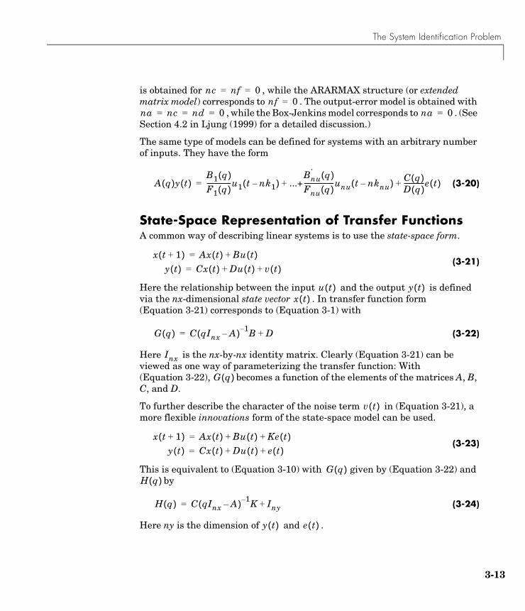
The System Identification Problem
3-13
is obtained for , while the ARARMAX structure (or extended matrix model) corresponds to . The output-error model is obtained with
, while the Box-Jenkins model corresponds to . (See Section 4.2 in Ljung (1999) for a detailed discussion.)
The same type of models can be defined for systems with an arbitrary number of inputs. They have the form
(3-20)
State-Space Representation of Transfer FunctionsA common way of describing linear systems is to use the state-space form.
(3-21)
Here the relationship between the input and the output is defined via the nx-dimensional state vector . In transfer function form (Equation 3-21) corresponds to (Equation 3-1) with
(3-22)
Here is the nx-by-nx identity matrix. Clearly (Equation 3-21) can be viewed as one way of parameterizing the transfer function: With (Equation 3-22), becomes a function of the elements of the matrices A, B, C, and D.
To further describe the character of the noise term in (Equation 3-21), a more flexible innovations form of the state-space model can be used.
(3-23)
This is equivalent to (Equation 3-10) with given by (Equation 3-22) and by
(3-24)
Here ny is the dimension of and .
nc nf 0= =nf 0=
na nc nd 0= = = na 0=
A q( )y t( )B1 q( )F1 q( )---------------u1 t nk1–( ) ...+
Bnu q( )Fnu q( )-------------------
·unu t nknu–( ) C q( )
D q( )-------------e t( )++=
x t 1+( ) Ax t( ) Bu t( )+=y t( ) Cx t( ) Du t( ) v t( )+ +=
u t( ) y t( )x t( )
G q( ) C qInx A–( ) 1– B D+=
Inx
G q( )
v t( )
x t 1+( ) Ax t( ) Bu t( ) Ke t( )+ +=y t( ) Cx t( ) Du t( ) e t( )+ +=
G q( )H q( )
H q( ) C qInx A–( ) 1– K Iny+=
y t( ) e t( )
3 Tutorial
3-14
It is often possible to set up a system description directly in the innovations form (Equation 3-23). In other cases, it might be preferable to describe first the nature of disturbances that act on the system. That leads to a stochastic state-space model
(3-25)
where and are stochastic processes with certain covariance properties. In stationarity and from an input-output view, (Equation 3-25) is equivalent to (Equation 3-23) if the matrix K is chosen as the steady-state Kalman gain. How to compute K from (Equation 3-25) is described in the Control System Toolbox documentation.
Continuous-Time State-Space ModelsIt is often easier to describe a system from physical modeling in terms of a continuous-time model. The reason is that most physical laws are expressed in continuous time as differential equations. Therefore, physical modeling typically leads to state-space descriptions like
(3-26)
Here, means the time derivative of . If the input is piece-wise constant over time intervals , then the relationship between and can be exactly expressed by (Equation 3-21) by taking
(3-27)
and associate with , etc. If you start with a continuous-time innovations form
(3-28)
the discrete-time counterpart is given by (Equation 3-23) where the relationships (Equation 3-27) still hold. The exact connection between and
is somewhat more complicated, though. An ad hoc solution is to use
x t 1+( ) Ax t( ) Bu t( ) w t( )+ +=y t( ) Cx t( ) Du t( ) e t( )+ +=
w t( ) e t( )
x· t( ) Fx t( ) Gu t( )+=y t( ) Hx t( ) Du t( ) v t( )+ +=
x· xkT t k 1+( )T<≤ u k[ ] u kT( )=
y k[ ] y kT( )=
A eFT;= B eFτG τ ;d
0
T
∫= C H=
y tT( ) y t[ ]
x· t( ) Fx t( ) Gu t( ) Ke t( )+ +=y t( ) Hx t( ) Du t( ) e t( )+ +=
KK
The System Identification Problem
3-15
(3-29)
in analogy with G and B. This is a good approximation for short sampling intervals T.
Estimating Impulse ResponsesConsider the descriptions (Equation 3-1) and (Equation 3-2). To directly estimate the impulse response coefficients, also in the multivariable case, it is suitable to define a high-order Finite Impulse Response (FIR) model
(3-30)
and estimate the g-coefficients by the linear least squares method. In fact, to check whether there are noncausal effects from input to output, for example, due to feedback from y in the generation of u (closed loop data), g for negative lags can also be estimated.
(3-31)
If u is white noise, the impulse response coefficients will be correctly estimated, even if the true dynamics from u to y are more complicated than these models. Therefore it is natural to filter both the output and the input through a filter that makes the input sequence as white as possible before estimating the g. This is the essence of correlation analysis for estimating impulse responses.
Estimating Spectra and Frequency FunctionsThis section describes methods that estimate the frequency functions and spectra (Equation 3-11) directly. The cross-covariance function between and is defined as analogously to (Equation 3-7). Its Fourier transform, the cross spectrum, , is defined analogously to (Equation 3-6). Provided that the input is independent of
, the relationship (Equation 3-1) implies the following relationships between the spectra.
K eFτK τ ;d
0
T
∫=
y t( ) g 0( )u t( ) g 1( )u t 1–( ) … g n( )u t n–( )+ + +=
y t( ) g m–( )u t m+( ) … g 1–( )u t 1+( ) g 0( )u t( )+ + + +=g 1( )u t 1–( ) … g n( )u t n–( )+ +
Ryu τ( )y t( ) u t( ) Ey t τ+( )u t( )
Φyu ω( )u t( )
v t( )
3 Tutorial
3-16
(3-32)
By estimating the various spectra involved, the frequency function and the disturbance spectrum can be estimated as follows.
Form estimates of the covariance functions (as defined in (Equation 3-7)) , , and , using
(3-33)
and analog expressions for the others. Then, form estimates of the corresponding spectra
(3-34)
and analogously for and . Here is the so-called lag window and M is the width of the lag window. The estimates are then formed as
(3-35)
This procedure is known as spectral analysis. (See Chapter 6 in Ljung (1999).)
Estimating Parametric ModelsGiven a description (Equation 3-10) and having observed the input-output data u, y, the (prediction) errors in (Equation 3-10) can be computed as
(3-36)
These errors are, for given data y and u, functions of G and H. These in turn are parameterized by the polynomials in (Equation 3-14) through (Equation 3-19) or by entries in the state-space matrices defined in
Φy ω( ) G eiω( )2Φu ω( ) Φv ω( )+=
Φyu ω( ) G eiω( )Φu ω( )=
Ry τ( ) Ryu τ( ) Ru τ( )
Ryu τ( ) 1N---- y t τ+( )u t( )
t 1=
N
∑=
Φˆ
y ω( ) Ryˆ τ( )WM τ( )e iωτ–
τ M–=
M
∑=
Φu Φyu WM τ( )
GN eiω( ) Φˆ
yu ω( )
Φˆ
u ω( )-------------------;= Φ
ˆv ω( ) Φ
ˆy ω( ) Φ
ˆyu ω( )
2
Φˆ
u ω( )-------------------------–=
e t( )
e t( ) H 1– q( ) y t( ) G q( )u t( )–[ ]=
The System Identification Problem
3-17
(Equation 3-26) through (Equation 3-29). The most common parametric identification method is to determine estimates of G and H by minimizing
(3-37)
that is
(3-38)
This is called a prediction error method. For Gaussian disturbances it coincides with the maximum likelihood method. (See Chapter 7 in Ljung (1999).)
A somewhat different philosophy can be applied to the ARX model (Equation 3-14). By forming filtered versions of the input
(3-39)
and by multiplying (Equation 3-14) with , , 2, , na and , , 2, , nb and summing over t, the noise in
(Equation 3-14) can be correlated out and solved for the dynamics. This gives the instrumental variable method, and are called the instruments. (See Section 7.6 in Ljung (1999).)
Subspace Methods for Estimating State-Space ModelsThe state-space matrices A, B, C, D, and K in (Equation 3-23) can be estimated directly, without first specifying any particular parameterization by efficient subspace methods. The idea behind this can be explained as follows: If the sequence of state vectors x(t) were known, together with y(t) and u(t), (Equation 3-23) would be a linear regression, and C and D could be estimated by the least squares method. Then e(t) could be determined, and treated as a known signal in (Equation 3-23), which then would be another linear regression model for A, B, and K. (One could also treat (Equation 3-21) as a linear regression for A, B, C, and D with y(t) and x(t+1) as simultaneous outputs, and find the joint process and measurement noises as the residuals from this regression. The Kalman gain K could then be computed from the
VN G H,( ) e2 t( )
t 1=
N
∑=
GN HN ],[ argmin e2 t( )
t 1=
N
∑=
N q( )s t( ) M q( )u t( )=
s t k–( ) k 1= …u t nk– 1 k–+( ) k 1= …
s t( )

3 Tutorial
3-18
Riccati equation.) Thus, once the states are known, the estimation of the state-space matrices is easy.
How to find the states x(t)? All states in representations like (Equation 3-23) can be formed as linear combinations of the k-step ahead predicted outputs (k = 1,2,...,n). It is thus a matter of finding these predictors, and then selecting a basis among them. The subspace methods form an efficient and numerically reliable way of determining the predictors by projections directly on the observed data sequences. See Sections 7.3 and 10.6 in Ljung (1999). For more details, see the references under n4sid in the reference pages.
The advice CommandA general command, advice, can be applied to any estimated model and to any data set,
advice(model)advice(data)
to provide the user with information about the quality of the model and characteristics, possibilities, and fallacies for the data set.
Data Representation and Nonparametric Model Estimation
3-19
Data Representation and Nonparametric Model EstimationThis and the following sections give an introduction to the basic functions in the System Identification Toolbox. Not all of the options available when using the functions are described here; see Chapter 4, “Function Reference,” and the online Help facility.
Data RepresentationThe observed output and input signals, and , are represented as column vectors y and u. Row k corresponds to sample number k. For multivariable systems, each input (output) component is represented as a column vector, so that u becomes an N-by-nu matrix (N = number of sampled observations, nu = number of input channels). The output-input data is collectively represented in the iddata format. This is the basic object for dealing with signals in the toolbox. It is used by most of the commands. It is created by
Data = iddata(y,u,Ts)
where y is a column vector or an N-by-ny matrix. The columns of y correspond to the different output channels. Similarly u is a column vector or an N-by-nu matrix containing the signals of the input channels. Ts is the sampling interval. This construction is sufficient for almost all purposes.
The data is then plotted by plot(Data) and portions of the data record are selected as in
ze = Data(1:300)
The signals in the output channels are retrieved by Data.OutputData or, for short, Data.y. Similarly the input signals are obtained by Data.InputData or Data.u.
For a time series (no input channels) use Data = iddata(y), or let u = [ ]. An iddata object can also contain just an input, by letting y = [ ].
You can change the sampling interval by using set(Data,'Ts',0.3) or, more simply, by
Data.Ts = 0.3
More details about the iddata object are given at the end of this section.
y t( ) u t( )
3 Tutorial
3-20
Correlation AnalysisThe correlation analysis procedure described in “Estimating Impulse Responses” on page 3-15 is implemented in the function impulse.
impulse(Data)
This function plots the estimated impulse response. Adding an argument 'sd' as in
impulse(Data,'sd',3)
also marks a confidence region corresponding to (in this case) three standard deviations. The result can be stored and replotted.
ir = impulse(Data)impulse(ir,'sd',3)
An alternative is the command step that plots the step response, calculated from the impulse estimate.
step(Data)
Spectral AnalysisThe function spa performs spectral analysis according to the procedure in (Equation 3-35) through (Equation 3-37).
g = spa(Data)
Here Data contains the output-input data in the iddata object as above. g is returned as an idfrd (identified frequency response data) model object, that contains the estimated frequency function and the estimated disturbance spectrum in (Equation 3-37), as well as estimated uncertainty covariances. The idfrd object is described in the idfrd reference page, but for normal use you do not have to bother about these details. The frequency function, or frequency response, G in g can be graphed by the function bode, ffplot, or nyquist. The noise spectrum is retrieved by g('n') ('n' for noise) so
g = spa(Data)bode(g)bode(g('n'))
performs the spectral analysis, and plots first G and then . The bode function gives logarithmic amplitude and frequency scales (in rad/s) and linear
GNΦˆ
v
Φv
Data Representation and Nonparametric Model Estimation
3-21
phase scale, while ffplot gives linear frequency scales (in Hz). The uncertainty of the estimates is displayed by adding the argument 'sd' as in
bode(g,'sd',3)
which displays, by dash-dotted lines, a confidence region around the estimate that corresponds (in this case) to three standard deviations. Adding an argument 'fill' shows the uncertainty region instead as a filled region.
bode(g,'sd',3,'fill')
Similarly
nyquist(g)
gives a Nyquist plot of the frequency function, that is, a plot of the real part versus the imaginary part of G.
If Data = y is a time series, that is, Data has no input channel, spa returns an estimate of the spectrum of that signal.
g= spa(y)ffplot(g)
In the computations (Equation 3-35) through (Equation 3-37), spa uses as a lag window the Hamming window for with a default length M equal to the minimum of 30 and a tenth of the number of data points. You can change this window size M to an arbitrary number using
g = spa(Data,M)
The rule is that as M increases, the estimated frequency functions show sharper details, but are also more affected by random disturbances. A typical sequence of commands that test different window sizes is
g10 = spa(Data,10)g25 = spa(Data,25)g50 = spa(Data,50)bode(g10, g25, g50)
An empirical transfer function estimate is obtained as the ratio of the output and input Fourier transforms with
g = etfe(Data)
W τ( )
3 Tutorial
3-22
This can also be interpreted as the spectral analysis estimate for a window size that is equal to the data length. For time series, etfe gives the periodogram as a spectral estimate. The function also allows some smoothing of the crude estimate; it can be a good alternative for signals and systems with sharp resonances. See Chapter 4, “Function Reference,” for more information.
Estimation of spectra and frequency functions involves a tradeoff between resolution and noise sensitivity. By resolution we mean the finest details (in rad/s) that can be distinguished in the estimate, while noise sensitivity describes how disturbances of different kinds give high variability in the estimates. The number M mentioned above is a way to control this tradeoff globally over the frequency range.
A useful complement to etfe and spa is the possibility of having frequency-dependent resolution, using the command spafdr,
g = spafdr(Data)g = spafrd(Data,Res,Freqs)
with the possibility of defining both the frequencies Freqs for which the estimate should be formed and the resolution Res for the different frequencies. See the spafdr reference page for more details.
Frequency Domain DataThe iddata object can also represent frequency-domain data, that is, input and output signals that are Fourier transforms of time-domain signals. Such data sets are useful in many contexts. You create a frequency-domain data set by
Data = iddata(Y,U,Ts,'Domain,'Frequency','freq',W)
where Y and U are the output and input Fourier transforms (N-by-ny and N-by-nu complex-valued matrices) and W is the vector of associated frequencies. That means that Y(kf,ky) is the frequency component of output number ky at frequency W(kf). Frequency-domain data can also easily be constructed from time-domain data, as in
dataf = fft(data)
A further way to handle frequency-domain information for model estimation is to define a frequency response data object (IDFRD) that contains the frequency-response data of a system, as in Equation 3-11:
datfr = idfrd(G,W,Ts)
Data Representation and Nonparametric Model Estimation
3-23
datfr = idfrd(G,W,Ts,'SpectrumData',Phiv)
Here G is the frequency response function, W is the vector of frequencies, and Ts is the sampling interval. Optionally, you can also include the additive output spectrum Phiv = .
You can also create a frequency-response data object from a model or from data by
datafr = idfrd(model)datafr = spafdr(Data)
(Compare the techniques on page 3-20.) While datafr can be seen as a nonparametric model of the system, it can also be seen as a more compact way of representing the data Data. This representation can be used to further estimate parametric models. Also, in many applications it is common to use frequency analyzers for data acquisition. They deliver data in the frequency-function form rather than as separate input and output signals, in a much more compact form.
More details of this are given on the reference pages for iddata and idfrd. The main message here is that the handling of data in time and frequency domain is essentially transparent. All estimation and representation commands that apply to time-domain data can also be used with the same syntax for frequency-domain data.
Two differences can be noted:
• Noise models cannot be estimated from frequency domain data.
• Frequency-domain data can handle representation of time-continuous signals (Ts = 0). This means that Y and U are the continuous-time Fourier transforms given at a finite number of frequencies.
More on the Data Representation in iddata
Some Bookkeeping FacilitiesThe input and output channels are given default names like y1, y2, u1, u2, etc. The channel names can be set by
set(Data,'InputName',{'Voltage','Current'},'OutputName','Temperature')
Φv ω( )
3 Tutorial
3-24
(two inputs and one output in this example) and these names will then follow the object and appear in all plots. The names are also inherited by models that are estimated from the data.
Similarly, channel units can be specified using the properties OutputUnit and InputUnit. These units, when specified, will be used in plots.
The time points associated with the data samples are determined by the sampling interval Ts and the time of the first sample, Tstart.
Data.Tstart = 24
The actual time-point values are given by the property SamplingInstants, as in
plot(Data.sa,Data.u)
for a plot of the input with correct time points. Autofill is used for all properties, and they are case insensitive. For easy writing, 'u' is synonymous to 'Input' and 'y' to 'Output' when you are referring to the properties.
Manipulating ChannelsAn easy way to set and retrieve channel properties is to use subscripting. The subscripts are defined as
Data(samples,outputs,inputs)
so Dat(:,3,:) is the data object obtained from Dat by keeping all input channels, but only output channel 3. (Trailing “:”s can be omitted so Dat(:,3,:) = Dat(:,3).)
You can also retrieve the channels by their names, so that
Dat(:,{'speed','flow'},[ ])
is the data object where the indicated output channels have been selected and no input channels are selected.
Moreover,
Dat1(101:200,[3 4],[1 3]) = Dat2(1001:1100,[1 2],[6 7])
will change samples 101 to 200 of output channels 3 and 4 and input channels 1 and 3 in the iddata object Dat1 to the indicated values from iddata object

Data Representation and Nonparametric Model Estimation
3-25
Dat2. The names and units of these channels are then also changed accordingly.
To add new channels, use horizontal concatenation of iddata objects.
Dat =[Dat1, Dat2];
See “Adding Channels” on page 3-26 or add the data record directly, so that
Dat.u(:,5) = u
will add a fifth input to Dat.
Nonequal SamplingThe property SamplingInstants gives the sampling instants of the data points. It can always be retrieved by get(Dat,'SamplingInstants') (or Dat.s) and is then computed from Dat.Ts and Dat.Tstart. SamplingInstants can also be set to an arbitrary vector of the same length as the data, so that nonequal sampling can be handled. Ts is then automatically set to [ ]. Most of the estimation routines, though, do not handle unequally sampled data.
Multiple ExperimentsThe iddata object can also store data from separate experiments. The property ExperimentName is used to separate the experiments. The number of data as well as the sampling properties can vary from experiment to experiment, but the input and output channels must be the same. (Use NaN to fill unmeasured channels in certain experiments.) The data records will be cell arrays where the cells contain data from each experiment.
You can define multiple experiments directly by letting the 'y' and 'u' properties as well as 'Ts' and 'Tstart' be cell arrays.
It is normally easier to create multiple-experiment data by merging experiments, as in
Dat = merge(Dat1,Dat2)
See the merge (iddata) reference page. Storing multiple experiments as one iddata object can be very useful to handle experimental data that has been collected on different occasions, or when a data set has been split up to remove “bad” portions of the data. All the toolbox’s routines accept multiple-experiment data.
3 Tutorial
3-26
Experiments can be retrieved by the command getexp, as in getexp(Dat,3) or getexp(Dat,'Period1'). They can also be set and retrieved by subscripting with a fourth index: Dat(:,:,:,3)} is experiment number 3 and Dat(:,:,:,{'Day1','Day4'}) retrieves the two experiments with the indicated names.
The subscripting can be combined: Dat(1:100,[2,3],[4:8],3) gives the 100 first samples of output channels 2 and 3 and input channels 4 to 8 of experiment number 3. It can also be used for subassignment.
Dat(:,:,:,''Run4') = Dat2
adds the data in Dat2 as a new experiment with name 'Run4'. See iddemo #9 for an illustration of how multiple experiments can be used.
iddata PropertiesType get(Dat) or see the iddata reference page for a complete list of iddata properties.
SubreferencingThe samples, outputs, and input channels can be referenced according to
Data(samples,outputs,inputs)
Use a colon (:) to denote all samples/channels and the empty matrix ([ ]) to denote no samples/channels. The channels can be referenced by number or by name. For several names you must use a cell array.
Dat2 = Dat(:,'y3',{'u1','u4'})Dat2 = Dat(:,3,[1 4])
Logical expressions also work.
Dat3 = Dat2(Dat2.sa>1.27&Dat2.sa<9.3)
selects the samples with time marks between 1.27 and 9.3.
Any subreferenced variable can also be assigned.
Data(1:10,1,1) = Dat1(101:110,2,3)
Adding ChannelsDat = [Dat1,Dat2,...,DatN]
Data Representation and Nonparametric Model Estimation
3-27
creates an iddata object Dat, consisting of the input and output channels in Dat1,... DatN. Default channel names ('u1', 'u2', 'y1', 'y2', etc.) are changed so that overlaps in names are avoided, and the new channels are added.
If Datk contains channels with user-specified names that are already present in the channels of Datj, j<k, these new channels are ignored.
Adding SamplesDat = [Dat1;Dat2;... ;DatN]
creates an iddata object Dat whose signals are obtained by stacking those of Datk on top of each other, that is,
Dat.y = [Dat1.y;Dat2.y; ... DatN.y]
and similarly for the inputs. The Datk objects must all have the same number of channels and experiments.
3 Tutorial
3-28
Parametric Model EstimationThe System Identification Toolbox contains several functions for parametric model estimation. They all share the same command structure.
m = function(Data,modstruc)m = ...function(Data,modstruc,'Property1',Value1,...'PropertyN',ValueN)
The argument Data is an iddata object that contains the output and input data sequences, while modstruc specifies the particular structure of the model to be estimated. The resulting estimated model is contained in m. It is a model object that stores various information. The model objects will be described in “Defining Model Structures” on page 3-39, but for most use of the toolbox, you do not have to consider the details of these objects. Just typing the model name
m
will give a concise display of the model. The command
present(m)
gives some more details, while
get(m)
gives a complete list of the model’s properties. The property values can be easily retrieved just by dot-referencing. For example,
m.par
retrieves the estimated parameters.
In the function call (...,'Property1', Value1,...,'PropertyN',ValueN) is a list of properties that can be assigned to affect the model structure, as well as the estimation algorithm. A list of typical properties is given at the end of this section. The model m is also immediately prepared for displaying and analyzing its characteristics as well as for transforming it to other representations, as in
bode(m)compare(Data,m)[A,B,C,D, K] = ssdata(m)
See “Examining Models” on page 3-57 for a detailed discussion of these possibilities.
Parametric Model Estimation
3-29
In the following, Data denotes an iddata object that contains the input output data as described in the previous section. It can also just contain an output signal, that is, a time series.
ARX ModelsTo estimate the parameters and of the ARX model (Equation 3-14), use the function arx.
m = arx(Data,[na nb nk])
Here na, nb, and nk are the corresponding orders and delays in (Equation 3-15) that define the exact model structure. The function arx implements the least squares estimation method, using QR-factorization for overdetermined linear equations.
An alternative is to use the Instrumental Variable (IV) method described in connection with (Equation 3-39). This is obtained with
m = iv4(Data,[na nb nk])
which gives an automatic (and approximately optimal) choice of the filters N and M in (Equation 3-39). (See the procedure (15.21)-(15.26) in Ljung (1999).)
Both arx and iv4 are applicable to arbitrary multivariable systems. If you have ny outputs and nu inputs, the orders are defined accordingly: na is an ny-by-ny matrix whose i-j entry gives the order of the polynomial that relates past values of to the current value of (that is, past values of up to are used when predicting . Similarly, the i-j entries of the ny-by-nu matrices nu and nk, respectively, give the order and delay from input number j when predicting output number i. (See “Multivariable ARX Models: the idarx Model” on page 3-43 and Chapter 4, “Function Reference,” for exact details.)
AR ModelsFor a single output signal , the counterpart of the ARX model is the AR model.
(3-40)
The arx command also covers this special case
m = arx(y,na)
ai bi
yj yi yj yj t na i j,( )–( )yi t )( )
y t( )
A q( )y t( ) e t( )=
3 Tutorial
3-30
but for scalar signals more options are offered by the command
m = ar(y,na)
which has an option that allows you to choose the algorithm from a group of several popular techniques for computing the least squares AR model. Among these are Burg’s method, a geometric lattice method, the Yule-Walker approach, and a modified covariance method. (See “Function Reference” on page 4-1 for details.) The counterpart of the iv4 command is
m = ivar(y,na)
which uses an instrumental variable technique to compute the AR part of a time series.
General Polynomial Black-Box ModelsBased on the prediction error method (Equation 3-38), you can construct models of basically any structure. For the general model (Equation 3-19), there is the function
m = pem(Data,nn)
where nn gives all the orders and delays.
nn = [na nb nc nd nf nk]
The nonzero orders of the model can also be defined as property name/property value pairs as in
m = pem(Data,'na',na,'nb',nb,'nc',nc,'nk',nk)
The input parameters are defined in “Polynomial Representation of Transfer Functions” on page 3-11. The pem command covers all cases of black-box linear system models. For the common special cases
m = armax(Data,[na nb nc nk])m = oe(Data,[nb nf nk])m = bj(Data,[nb nc nd nf nk])
can be used. These handle the model structures (Equation 3-16), (Equation 3-17) and (Equation 3-18), respectively.
All the routines also cover single-output, multiinput systems of the type
Parametric Model Estimation
3-31
(3-41)
where nb, nf, and nk are row vectors of the same lengths as the number of input channels containing each of the orders and delays
nb = [nb1 ... nbnu];nf = [nf1 ... nfnu];nk = [nk1 ... nknu];
These parameter estimation routines require an iterative search for the minimum of the function (Equation 3-39). This search uses a special startup procedure based on least squares and instrumental variables (the details are given as Equation (10.79) in Ljung (1999)). From the initial estimate, a Gauss-Newton minimization procedure is carried out until the norm of the Gauss-Newton direction is less than a certain tolerance. See Ljung (1999), Section 11.2 or Dennis and Schnabel (1983) for details. See also the entry at the end of this section on optional variables associated with the search.
The estimation routines also return the estimated covariance matrix of the estimated parameter vector as part of m. This reflects the reliability of the estimates. The covariance matrix estimate is computed under the assumption that it is possible to obtain a “true” description in the given structure.
The routines pem, armax, oe, and bj can also be started at any initial value mi that is a model object by replacing nn by mi. For example,
m = pem(Data,mi)
While the search is typically initialized using the built-in startup procedure giving just orders and delays (as described above), the ability to force a specific initial condition is useful in several contexts. Some examples are mentioned in “Initial Parameter Values” on page 3-97.
Information about how the minimization progresses can be supplied to the MATLAB Command Window by the property trace. See the list at the end of this section.
Process ModelsFor process control applications, often simple continuous-time models are used, consisting of static gain, time constant(s), and a possible dead time (time delay). Such model are estimated by commands of the kind
A q( )y t( )B1 q( )F1 q( )---------------u1 t nk1–( ) …
Bnu q( )Fnu q( )-------------------unu t nknu–( ) C q( )
D q( )-------------e t( )+ + +=
3 Tutorial
3-32
m = pem(Data,'P1D')
where P1D here indicates one pole (time constant) and a delay. See “Process Models: the idproc Model” on page 3-41 and the reference page for Purpose for more details.
State-Space Models
Black-Box, Discrete Time ParameterizationsSuppose first that there is no particular knowledge about the internal structure of the discrete-time state-space model (Equation 3-15). Any linear model is sought. A simple approach then is to use
m = pem(Data)
This estimates a state-space model of an order (among 1 to 10) that seems reasonable.
To find a black-box model of a certain order n, use
m = pem(Data,n)
To get a plot, from which the order can be determined among a list of orders nn = [n1,n2,...,nN], use
m = pem(Data,'nx',nn)
All these black-box models are initialized by the subspace method n4sid. To obtain the estimate from this routine, use
m = n4sid(Data,n)
Arbitrarily Structured Models in Discrete and Continuous TimeFor state-space models of given structure, most of the effort involved relates to defining and manipulating the structure. This is discussed in “Structured State-Space Models with Free Parameters: the idss Model” on page 3-48. Once the structure is defined as ms, you can estimate its parameters with
m = pem(Data,ms)
When the systems are multioutput, the following criterion is used for the minimization,
Parametric Model Estimation
3-33
(3-42)
which is the maximum likelihood criterion for Gaussian noise with unknown covariance matrix.
The numerical minimization of the prediction error criterion (Equation 3-39) or (Equation 3-42) can be a difficult problem for general model parameterizations. The criterion, as a function of the free parameters, can define a complicated surface with many local minima, narrow valleys, and so on. This may require substantial interaction from the user, in providing reasonable initial parameter values, and also by freezing certain parameter values (using the property FixedParameters) while allowing others to be free. Note that pem easily allows the freezing of any parameters to their current/nominal values. The model structure can also be directly manipulated as described in “Structured State-Space Models with Free Parameters: the idss Model” on page 3-48. A procedure that is often used for state-space models is to allow the noise parameter in the K matrix free only when a reasonable model of the dynamic part has been obtained.
Optional VariablesThe estimation functions accept a list of property name/property value pairs that may affect both the model structure and the estimation algorithm. For complete lists of these properties, see algorithm properties, idarx, idmodel, idpoly, idproc, idss, and idgrey in the “Function Reference” on page 4-1. Some of them are listed here. Note that any property, as well as values that are strings, can be entered as any unambiguous, case-insensitive abbreviation, as is
m = pem(Data,mi,'fo','si').
Note Algorithm is a property of idmodel. Any algorithm property can be separately set as above. Also, if you have a standard algorithm set up that you prefer, you can set those properties simultaneously as inm = pem(Data,mi,'alg',myalg).
det e t( )eT t( )
t 1=
N
∑
3 Tutorial
3-34
Note The algorithm properties, like all other model properties, are inherited by the resulting model m. If you continue the estimation using m as the initial model, all previously set algorithm features will thus apply, unless you specify otherwise.
Applying to All Estimation MethodsThe following properties apply to all estimation methods:
• Focus
• MaxSize
• FixedParameter
Focus: This property affects the weighting applied to the fit between the model and the data. It can be used to assure that the model approximates the true system well over certain frequency intervals. Focus can assume the following values:
• Prediction: This is the default and means that the model is determined by minimizing the prediction errors. It corresponds to a frequency weighting that is given by the input spectrum times the inverse noise model. Typically, this favors a good fit at high frequencies. From a statistical variance point of view, this is the optimal weighting, but then the approximation aspects (bias) of the fit are neglected.
• Simulation: This means that frequency weighting of the transfer function fit is given by the input spectrum. Frequency ranges where the input has considerable power will thus be better described by the model. In other words, the model approximation is such that the model will produce as good simulations as possible, when applied to inputs with the same spectra as used for the estimation. For models that have no disturbance model (A=C=D for idpoly models and K=0 for idss models) there is no difference between the simulation and prediction values. For models with a disturbance description, this is estimated by a prediction error method, keeping the estimated transfer function from input to output fixed. The resulting model is guaranteed to be stable.
• Stability: The algorithm is modified so that a stable model is guaranteed, but the weighing still corresponds to prediction.
Parametric Model Estimation
3-35
• A frequency range for passbands. Focus = [w1 w2] where the interval defines a passband (in rad/s) for the signals. By letting focus have several rows, filtering with several passbands can be defined. The model fit will then be focused to the passband(s) defined in this way.
• Any SISO linear filter. Then the transfer function from input to output is determined by a frequency fit with this filter times the input spectrum as weighting function. The noise model is determined by a prediction error method, keeping the transfer function estimate fixed. To obtain a good model fit over a special frequency range, the filter should thus be chosen with a passband over this range. For a model with no disturbance model, the result is the same as first applying prefiltering to data using idfilt. The filter can be specified as
- Any single-input single-output idmodel
- An ss, tf, or zpk model from the Control System Toolbox
- {A,B,C,D} with the state-space matrices for the filter (notice the curly brackets)
- {numerator, denominator} with the transfer function numerator/denominator of the filter
MaxSize: No matrix with more than MaxSize elements is formed by the algorithm. Instead, for loops are used. MaxSize will thus decide the memory/speed tradeoff, and can prevent slow use of virtual memory. MaxSize can be any positive integer, but the input-output data must contain fewer than MaxSize elements. The default value of MaxSize is Auto, which means that the value is determined in the M-file idmsize. This file can be edited by the user to optimize speed on a particular computer. See also “Memory/Speed Tradeoffs” on page 3-96.
FixedParameter: A list of parameters that will be kept fixed to the nominal/initial values and not estimated. This is a vector of integers containing the indices of the fixed parameters, or a cell array of parameter names. If names are used, wildcard entries apply, which may be convenient if you have groups of parameters in your model. See the reference page for Algorithm Properties.
Algorithm Properties That Apply to n4sid, Estimating State-Space ModelsThe properties that apply to subspace model estimation are
• N4Weight
3 Tutorial
3-36
• N4Horizon
These properties then also apply to pem for estimating black-box state-space models, since pem is then initialized by the n4sid estimate.
N4Weight: This property determines some weighting matrices used in the singular-value decomposition that is a central step in the algorithm. Two choices are offered: moesp, which corresponds to the MOESP algorithm by Verhaegen and cva, which is the canonical variable algorithm by Larimore. The default value is N4Weight = Auto, which gives an automatic choice between the two options.
N4Horizon: Determines the prediction horizons forward and backward used by the algorithm. This is a row vector with three elements: N4Horizon =[r sy su], where r is the maximum forward prediction horizon, that is, the algorithm uses up to r-step ahead predictors. sy is the number of past outputs, and su is the number of past inputs that are used for the predictions. See Ljung (1999), pages 345-348. These numbers can have a substantial influence on the quality of the resulting model, and there are no simple rules for choosing them. Making N4Horizon a k-by-3 matrix means that each row of N4Horizon is tried and the value that gives the best (prediction) fit to data is selected. If you specify only one column in N4Horizon, the interpretation is r=sy=su. The default choice is N4Horizon = Auto, which uses the Akaike Information Criterion (AIC) for the selection of sy and su. See the reference page for n4sid for literature references.
Properties That Apply to Estimation Methods Using Iterative Search for Minimizing a Criterion The properties that govern the iterative search are
• Trace
• LimitError
• MaxIter
• Tolerance
• SearchDirection
• Advanced
These properties apply to armax, bj, oe, and pem.
Parametric Model Estimation
3-37
Trace: This property determines the information about the iterative search that is provided to the MATLAB Command Window:
• Trace = Off: No information is written to the screen.
• Trace = On: Information about criterion values and the search process is given for each iteration.
• Trace= Full: The current parameter values and the search direction are also given (except in the “free” SSParameterization case for idss models).
LimitError: This variable determines how the criterion is modified from quadratic to one that gives linear weight to large errors. Errors larger than LimitError times the estimated standard deviation will carry a linear weight in the criteria. The default value of LimitError is 1.6. LimitError = 0 disables the robustification and leads to a purely quadratic criterion. The standard deviation is estimated robustly as the median of the absolute deviations from the median, divided by 0.7. (See Equations (15.9) and (15.10) in Ljung (1999).)
MaxIter: The maximum number of iterations performed during the search for minimum. The iterations stop when MaxIter is reached or some other stopping criterion is satisfied. The default value of MaxIter is 20. Setting MaxIter = 0 returns the result of the startup procedure. The actual number of iterations used is given by the property EstimationInfo.Iterations.
Tolerance: Based on the Gauss-Newton vector computed at the current parameter value, an estimate is made of the expected improvement of the criterion at the next iteration. When this expected improvement is less than Tolerance %, the iterations are stopped. The default value is 0.01.
SearchDirection: The direction along which a line search is performed to find a lower value of the criterion function. It can assume the following values:
• gn: The Gauss-Newton direction (inverse of the Hessian times the gradient direction). If no improvement is found along this direction, the gradient direction is also tried out.
• gns: A regularized version of the Gauss-Newton direction. Eigenvalues less than pinvtol of the Hessian are neglected, and the Gauss-Newton direction is computed in the remaining subspace. (pinvtol is part of the 'advanced' field: See the Algorithm Properties reference page.
3 Tutorial
3-38
• lm: The Levenberg-Marquardt method is used. This means that the next parameter value is -pinv(H+d*I)*grad from the previous one, where H is the Hessian, I is the identity matrix, and grad is the gradient. d is a number that is increased until a lower value of the criterion is found.
• Auto: A choice between the above is made in the algorithm. This is the default choice.
One property of the returned model is EstimationInfo. That is a structure that contains useful information about the estimation process. See the EstimationInfo reference page for a list of fields.
Another important option is InitialState. See “Initial State” on page 3-98.
For the spectral analysis estimate, you can compute the frequency functions at arbitrary frequencies. If the frequencies are specified in a row vector w, then
g = spa(z,M,w)
results in g being computed at these frequencies. You can generate logarithmically spaced frequencies using the MATLAB logspace function. For example,
w = logspace(-3,pi,128)
Defining Model Structures
3-39
Defining Model StructuresSince the System Identification Toolbox handles a wide variety of different model structures, it is important that these can be defined in a flexible way. In the previous section you saw how models are automatically produced in the right form by the various estimation routines, arx, iv4, oe, bj, armax, and pem, if you just specify model orders and delays.
This section describes how model structures and models can be directly defined. This may be required, for example, when creating a model for simulation. Also, it many be necessary to define model structures that are not of black-box type, but contain more detailed internal structure, reflecting some physical insights into how the system works.
The general way of representing models and model structures in the System Identification Toolbox is by various model objects. This section introduces the commands (apart from the parametric estimation functions themselves) that create these different models.
The model objects will contain a number of properties. For any model you can type
get(m)
to see a list of the model’s properties, and
set(m)
to see what the assignable values are. See the get and set reference pages. Each property value can easily also be retrieved by subreferencing as in
m.A
and set as in
m.b(3) = 27
See the idmodel reference page for complete property lists. Here only examples are given. Note that it is sufficient to use any case-insensitive, unambiguous abbreviation of the property names. Also, 'u' is short for 'input' and 'y' is short for 'output'.

3 Tutorial
3-40
Polynomial Black-Box Models: the idpoly ModelThe general input-output form (Equation 3-19)
(3-43)
is defined by the five polynomials A(q), B(q), C(q), D(q), and F(q). These are represented in the standard MATLAB format for polynomials. Polynomial coefficients are stored as row vectors ordered by descending powers. For example, the polynomial
is represented as
A = [1 a1 a2 ... an]
Delays in the system are indicated by leading zeros in the polynomial. For example, the ARX model
(3-44)
is represented by the polynomials
A = [1 -1.5 0.7]B = [0 0 2.5 0.9]
The idpoly representation of (Equation 3-43) is now created by the command
m = idpoly(A,B,C,D,F,lam,T)
lam is the variance of the white noise source , and T is the sampling interval. Trailing arguments can be omitted for default values. The system (Equation 3-44) can, for example, be represented by
m = idpoly([1 -1.5 0.7],[0 0 2.5 0.9])
In the multiinput case (Equation 3-41), B and F are matrices whose row number k corresponds to the kth input. For time series (no input signal), set B = [] and F = []. (See “Time-Series Modeling” on page 3-92 for more details on time series.) The command idpoly can also be used to define continuous-time systems. See the idpoly reference page for details.
A q( )y t( ) B q( )F q( )------------u t nk–( ) C q( )
D q( )-------------e t( )+=
A q( ) 1 a1q 1– a2q 2– … anq n–+ + + +=
B q( )
y t( ) 1.5y t 1–( )– 0.7y t 2–( )+ 2.5u t 2–( ) 0.9u t 3–( )+=
e t( )
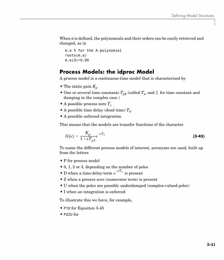
Defining Model Structures
3-41
When m is defined, the polynomials and their orders can be easily retrieved and changed, as in
m.a % for the A-polynomialroots(m.a)m.a(3)=0.95
Process Models: the idproc ModelA process model is a continuous-time model that is characterized by
• The static gain Kp
• One or several time constants Tpk (called Tw and for time constant and damping in the complex case.)
• A possible process zero Tz
• A possible time delay (dead time) Td
• A possible enforced integration
This means that the models are transfer functions of the character
(3-45)
To name the different process models of interest, acronyms are used, built up from the letters
• P for process model
• 0, 1, 2 or 3, depending on the number of poles
• D when a time-delay term is present
• Z when a process zero (numerator term) is present
• U when the poles are possibly underdamped (complex-valued poles)
• I when an integration is enforced
To illustrate this we have, for example,
• P1D for Equation 3-45
• P2ZU for
ζ
G s( )Kp
1 sTp1+----------------------e
sTd–=
esTd–
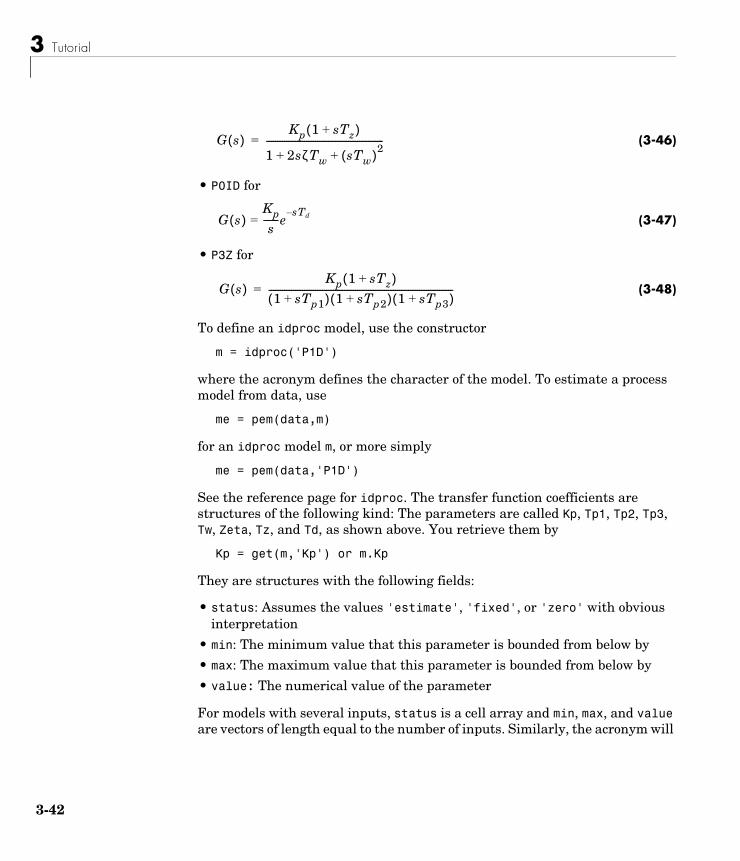
3 Tutorial
3-42
(3-46)
• P0ID for
(3-47)
• P3Z for
(3-48)
To define an idproc model, use the constructor
m = idproc('P1D')
where the acronym defines the character of the model. To estimate a process model from data, use
me = pem(data,m)
for an idproc model m, or more simply
me = pem(data,'P1D')
See the reference page for idproc. The transfer function coefficients are structures of the following kind: The parameters are called Kp, Tp1, Tp2, Tp3, Tw, Zeta, Tz, and Td, as shown above. You retrieve them by
Kp = get(m,'Kp') or m.Kp
They are structures with the following fields:
• status: Assumes the values 'estimate', 'fixed', or 'zero' with obvious interpretation
• min: The minimum value that this parameter is bounded from below by
• max: The maximum value that this parameter is bounded from below by
• value: The numerical value of the parameter
For models with several inputs, status is a cell array and min, max, and value are vectors of length equal to the number of inputs. Similarly, the acronym will
G s( )Kp 1 sTz+( )
1 2sζTw sTw( )2+ +-----------------------------------------------------=
G s( )Kps
-------esTd–
=
G s( )Kp 1 sTz+( )
1 sTp1+( ) 1 sTp2+( ) 1 sTp3+( )-----------------------------------------------------------------------------------=
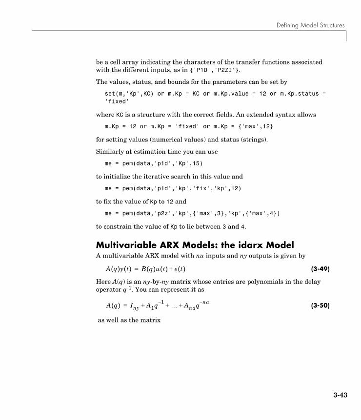
Defining Model Structures
3-43
be a cell array indicating the characters of the transfer functions associated with the different inputs, as in {'P1D','P2ZI'}.
The values, status, and bounds for the parameters can be set by
set(m,'Kp',KC) or m.Kp = KC or m.Kp.value = 12 or m.Kp.status = 'fixed'
where KC is a structure with the correct fields. An extended syntax allows
m.Kp = 12 or m.Kp = 'fixed' or m.Kp = {'max',12}
for setting values (numerical values) and status (strings).
Similarly at estimation time you can use
me = pem(data,'p1d','Kp',15)
to initialize the iterative search in this value and
me = pem(data,'p1d','kp','fix','kp',12)
to fix the value of Kp to 12 and
me = pem(data,'p2z','kp',{'max',3},'kp',{'max',4})
to constrain the value of Kp to lie between 3 and 4.
Multivariable ARX Models: the idarx ModelA multivariable ARX model with nu inputs and ny outputs is given by
(3-49)
Here A(q) is an ny-by-ny matrix whose entries are polynomials in the delay operator q-1. You can represent it as
(3-50)
as well as the matrix
A q( )y t( ) B q( )u t( ) e t( )+=
A q( ) Iny A1q 1– … Anaq na–+ + +=
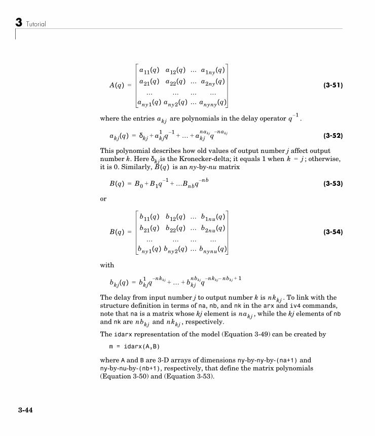
3 Tutorial
3-44
(3-51)
where the entries are polynomials in the delay operator .
(3-52)
This polynomial describes how old values of output number j affect output number k. Here is the Kronecker-delta; it equals 1 when ; otherwise, it is 0. Similarly, is an ny-by-nu matrix
(3-53)
or
(3-54)
with
The delay from input number j to output number k is . To link with the structure definition in terms of na, nb, and nk in the arx and iv4 commands, note that na is a matrix whose kj element is , while the kj elements of nb and nk are and , respectively.
The idarx representation of the model (Equation 3-49) can be created by
m = idarx(A,B)
where A and B are 3-D arrays of dimensions ny-by-ny-by-(na+1) and ny-by-nu-by-(nb+1), respectively, that define the matrix polynomials (Equation 3-50) and (Equation 3-53).
A q( )
a11 q( ) a12 q( ) … a1ny q( )
a21 q( ) a22 q( ) … a2ny q( )
… … … …any1 q( ) any2 q( ) … anyny q( )
=
akj q 1–
akj q( ) δkj akj1 q 1– … akj
nakjqnakj–
+ + +=
δkj k j=B q( )
B q( ) B0 B1q 1– …Bnbq nb–+ +=
B q( )
b11 q( ) b12 q( ) … b1nu q( )
b21 q( ) b22 q( ) … b2nu q( )
… … … …bny1 q( ) bny2 q( ) … bnynu q( )
=
bkj q( ) bkj1 q
nkkj–… bkj
nbkjqnkkj nbkj– 1+–
+ +=
nkkj
nakjnbkj nkkj
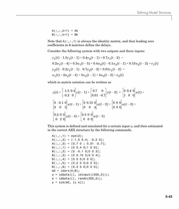
Defining Model Structures
3-45
A(:,:,k+1) = Ak B(:,:,k+1) = Bk
Note that A(:,:,1) is always the identity matrix, and that leading zero coefficients in B matrices define the delays.
Consider the following system with two outputs and three inputs:
which in matrix notation can be written as
This system is defined and simulated for a certain input u, and then estimated in the correct ARX structure by the following commands.
A(:,:,1) = eye(2);A(:,:,2) = [-1.5 0.4; -0.2 0];A(:,:,3) = [0.7 0 ; 0.01 -0.7];B(:,:,1) = [0 0.4 0;1 0 0];B(:,:,2) = [0 -0.1 0;0 0 3];B(:,:,3) = [0 0.15 0;0 0 4];B(:,:,4) = [0 0 0;0 0 0];B(:,:,5) = [0.2 0 0;0 2 0];B(:,:,6) = [0.3 0 0;0 0 0];m0 = idarx(A,B);u = iddata([], idinput([200,3]));e = iddata([], randn(200,2));y = sim(m0, [u e]);
y1 t( ) 1.5y1 t 1–( )– 0.4y2 t 1–( ) 0.7y1 t 2–( )+ + =
0.2u1 t 4–( ) 0.3u1 t 5–( ) 0.4u2 t( ) 0.1u2 t 1–( )– 0.15u2 t 2–( ) e1 t( )+ + + +
y2 t( ) 0.2y1 t 1–( )– 0.7y2 t 2–( )– 0.01y1 t 2–( )+ =
u1 t( ) 2u2 t 4–( ) 3u3 t 1–( ) 4u3 t 2–( ) e2 t( )+ + + +
y t( ) 1.5– 0.40.2– 0
y t 1–( ) 0.7 00.01 0.7–
y t 2–( )+ + 0 0.4 01 0 0
u t( ) +=
0 0.1– 00 0 3
u t 1–( ) 0 0.15 00 0 4
u t 2–( ) 0 0 00 0 0
u t 3–( )+ + +
0.2 0 00 2 0
u t 4–( ) 0.3 0 00 0 0
u t 5–( )+
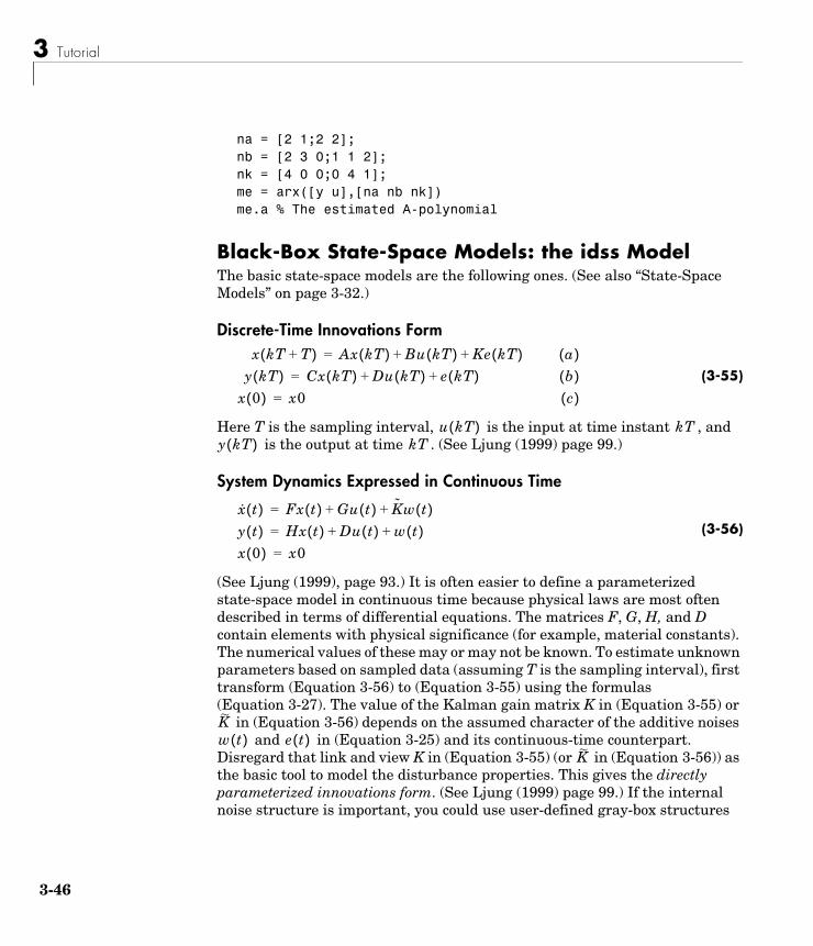
3 Tutorial
3-46
na = [2 1;2 2];nb = [2 3 0;1 1 2];nk = [4 0 0;0 4 1];me = arx([y u],[na nb nk])me.a % The estimated A-polynomial
Black-Box State-Space Models: the idss ModelThe basic state-space models are the following ones. (See also “State-Space Models” on page 3-32.)
Discrete-Time Innovations Form
(3-55)
Here T is the sampling interval, is the input at time instant , and is the output at time . (See Ljung (1999) page 99.)
System Dynamics Expressed in Continuous Time
(3-56)
(See Ljung (1999), page 93.) It is often easier to define a parameterized state-space model in continuous time because physical laws are most often described in terms of differential equations. The matrices F, G, H, and D contain elements with physical significance (for example, material constants). The numerical values of these may or may not be known. To estimate unknown parameters based on sampled data (assuming T is the sampling interval), first transform (Equation 3-56) to (Equation 3-55) using the formulas (Equation 3-27). The value of the Kalman gain matrix K in (Equation 3-55) or
in (Equation 3-56) depends on the assumed character of the additive noises and in (Equation 3-25) and its continuous-time counterpart.
Disregard that link and view K in (Equation 3-55) (or in (Equation 3-56)) as the basic tool to model the disturbance properties. This gives the directly parameterized innovations form. (See Ljung (1999) page 99.) If the internal noise structure is important, you could use user-defined gray-box structures
x kT T+( ) Ax kT( ) Bu kT( ) Ke kT( )+ += a( )y kT( ) Cx kT( ) Du kT( ) e kT( )+ += b( )
x 0( ) x0= c( )
u kT( ) kTy kT( ) kT
x· t( ) Fx t( ) Gu t( ) Kw t( )+ +=y t( ) Hx t( ) Du t( ) w t( )+ +=x 0( ) x0=
K~
w t( ) e t( )K~
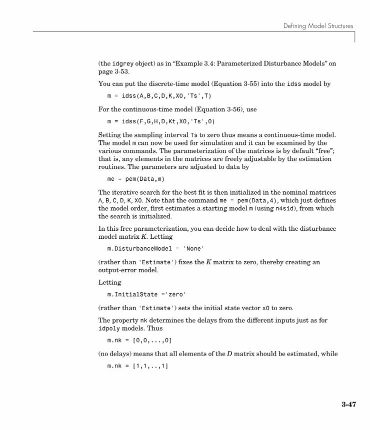
Defining Model Structures
3-47
(the idgrey object) as in “Example 3.4: Parameterized Disturbance Models” on page 3-53.
You can put the discrete-time model (Equation 3-55) into the idss model by
m = idss(A,B,C,D,K,X0,'Ts',T)
For the continuous-time model (Equation 3-56), use
m = idss(F,G,H,D,Kt,X0,'Ts',0)
Setting the sampling interval Ts to zero thus means a continuous-time model. The model m can now be used for simulation and it can be examined by the various commands. The parameterization of the matrices is by default “free”; that is, any elements in the matrices are freely adjustable by the estimation routines. The parameters are adjusted to data by
me = pem(Data,m)
The iterative search for the best fit is then initialized in the nominal matrices A, B, C, D, K, X0. Note that the command me = pem(Data,4), which just defines the model order, first estimates a starting model m (using n4sid), from which the search is initialized.
In this free parameterization, you can decide how to deal with the disturbance model matrix K. Letting
m.DisturbanceModel = 'None'
(rather than 'Estimate') fixes the K matrix to zero, thereby creating an output-error model.
Letting
m.InitialState ='zero'
(rather than 'Estimate') sets the initial state vector x0 to zero.
The property nk determines the delays from the different inputs just as for idpoly models. Thus
m.nk = [0,0,...,0]
(no delays) means that all elements of the D matrix should be estimated, while
m.nk = [1,1,..,1]
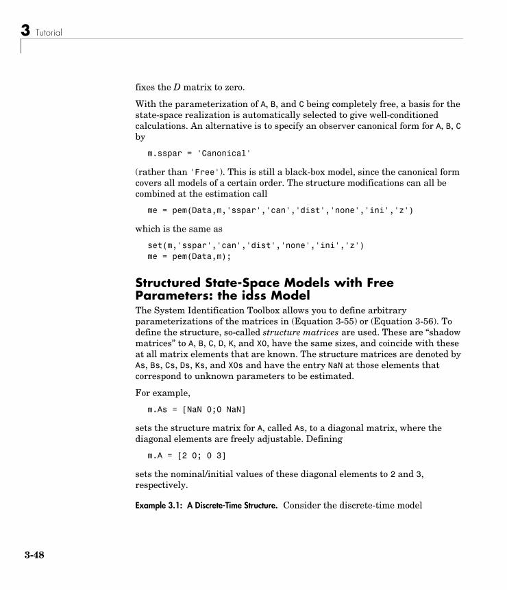
3 Tutorial
3-48
fixes the D matrix to zero.
With the parameterization of A, B, and C being completely free, a basis for the state-space realization is automatically selected to give well-conditioned calculations. An alternative is to specify an observer canonical form for A, B, C by
m.sspar = 'Canonical'
(rather than 'Free'). This is still a black-box model, since the canonical form covers all models of a certain order. The structure modifications can all be combined at the estimation call
me = pem(Data,m,'sspar','can','dist','none','ini','z')
which is the same as
set(m,'sspar','can','dist','none','ini','z')me = pem(Data,m);
Structured State-Space Models with Free Parameters: the idss ModelThe System Identification Toolbox allows you to define arbitrary parameterizations of the matrices in (Equation 3-55) or (Equation 3-56). To define the structure, so-called structure matrices are used. These are “shadow matrices” to A, B, C, D, K, and X0, have the same sizes, and coincide with these at all matrix elements that are known. The structure matrices are denoted by As, Bs, Cs, Ds, Ks, and X0s and have the entry NaN at those elements that correspond to unknown parameters to be estimated.
For example,
m.As = [NaN 0;0 NaN]
sets the structure matrix for A, called As, to a diagonal matrix, where the diagonal elements are freely adjustable. Defining
m.A = [2 0; 0 3]
sets the nominal/initial values of these diagonal elements to 2 and 3, respectively.
Example 3.1: A Discrete-Time Structure. Consider the discrete-time model
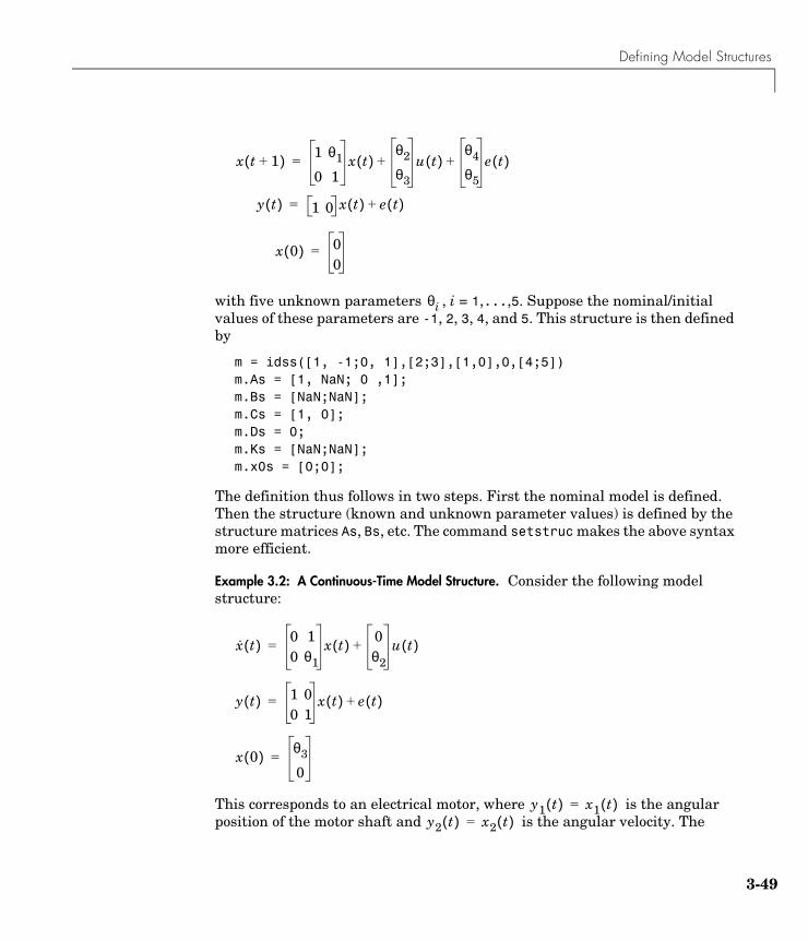
Defining Model Structures
3-49
with five unknown parameters , i = 1,...,5. Suppose the nominal/initial values of these parameters are -1, 2, 3, 4, and 5. This structure is then defined by
m = idss([1, -1;0, 1],[2;3],[1,0],0,[4;5])m.As = [1, NaN; 0 ,1];m.Bs = [NaN;NaN];m.Cs = [1, 0];m.Ds = 0;m.Ks = [NaN;NaN];m.x0s = [0;0];
The definition thus follows in two steps. First the nominal model is defined. Then the structure (known and unknown parameter values) is defined by the structure matrices As, Bs, etc. The command setstruc makes the above syntax more efficient.
Example 3.2: A Continuous-Time Model Structure. Consider the following model structure:
This corresponds to an electrical motor, where is the angular position of the motor shaft and is the angular velocity. The
x t 1+( ) 1 θ1
0 1x t( )
θ2
θ3
u t( )θ4
θ5
e t( )+ +=
y t( ) 1 0 x t( ) e t( )+=
x 0( ) 00
=
θi
x· t( ) 0 10 θ1
x t( ) 0θ2
u t( )+=
y t( ) 1 00 1
x t( ) e t( )+=
x 0( ) θ3
0=
y1 t( ) x1 t( )=y2 t( ) x2 t( )=

3 Tutorial
3-50
parameter is the inverse time constant of the motor and is the static gain from the input to the angular velocity. (See Example 4.1 in Ljung (1999).) The motor is at rest at time 0 but at an unknown angular position. Suppose that is around -1 and is around 0.25. If you also know that the variance of the errors in the position measurement is 0.01 and in the angular velocity measurements is 0.1, you can then define an idss model using
m = idss([0 1;0 ... -1],[0;0.25],eye(2),[0;0],zeros(2,2),[0;0],'Ts',0)
m.as = [0 1; 0 NaN]m.bs = [0 ;NaN]m.cs = m.cm.ds = m.dm.ks = m.km.x0s = [NaN;0]m.noisevar = [0.01 0; 0 0.1]
The structure m can now be used to estimate the unknown parameters from observed data
Data = iddata([y1 y2], u, 0.1)
by
model = pem(Data,m)
The iterative search for minimum is then initialized at the parameters in the nominal model m. The continuous-time model is automatically sampled to agree with the sampling interval of the data. The structure can also be used to simulate the system above with sampling interval T = 0.1 for input u and noise realization e.
e = randn(300,2)u = idinput(300);simdat = iddata([],[u e],'Ts',0.1);y = sim(m,simdat) % The continuous system will automatically be
% sampled using Ts = 0.1.
The nominal parameter values are then used, and the noise sequence is scaled according to the matrix m.noisevar.
When estimating models, you can try a number of “neighboring” structures, such as “what happens if I fix this parameter to a certain value” or “what
θ1– θ2 θ1⁄–
θ1 θ2
θi
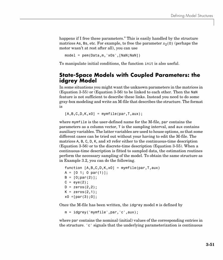
Defining Model Structures
3-51
happens if I free these parameters.” This is easily handled by the structure matrices As, Bs, etc. For example, to free the parameter x2(0) (perhaps the motor wasn’t at rest after all), you can use
model = pem(Data,m,'x0s',[NaN;NaN])
To manipulate initial conditions, the function init is also useful.
State-Space Models with Coupled Parameters: the idgrey ModelIn some situations you might want the unknown parameters in the matrices in (Equation 3-55) or (Equation 3-56) to be linked to each other. Then the NaN feature is not sufficient to describe these links. Instead you need to do some gray-box modeling and write an M-file that describes the structure. The format is
[A,B,C,D,K,x0] = mymfile(par,T,aux);
where mymfile is the user-defined name for the M-file, par contains the parameters as a column vector, T is the sampling interval, and aux contains auxiliary variables. The latter variables are used to house options, so that some different cases can be tried out without your having to edit the M-file. The matrices A, B, C, D, K, and x0 refer either to the continuous-time description (Equation 3-56) or to the discrete-time description (Equation 3-55). When a continuous-time description is fitted to sampled data, the estimation routines perform the necessary sampling of the model. To obtain the same structure as in Example 3.2, you can do the following.
function [A,B,C,D,K,x0] = mymfile(par,T,aux)A = [0 1; 0 par(1)]; B = [0;par(2)];C = eye(2);D = zeros(2,2);K = zeros(2,1);x0 =[par(3);0];
Once the M-file has been written, the idgrey model m is defined by
m = idgrey('mymfile',par,'c',aux);
where par contains the nominal (initial) values of the corresponding entries in the structure. 'c' signals that the underlying parameterization is continuous
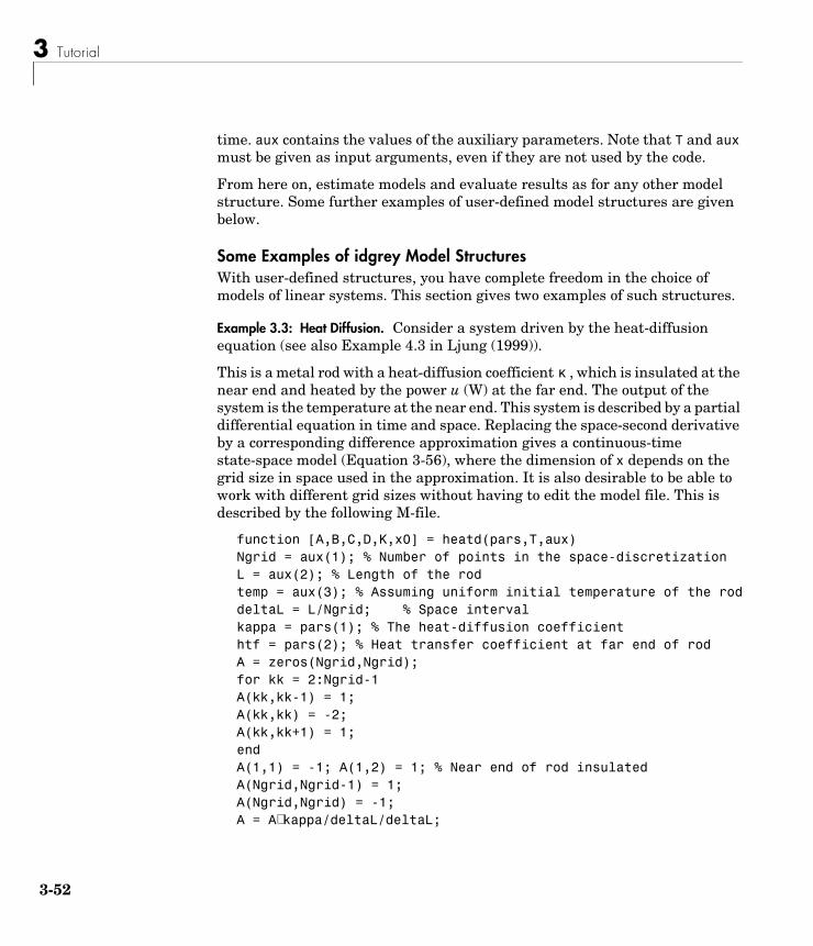
3 Tutorial
3-52
time. aux contains the values of the auxiliary parameters. Note that T and aux must be given as input arguments, even if they are not used by the code.
From here on, estimate models and evaluate results as for any other model structure. Some further examples of user-defined model structures are given below.
Some Examples of idgrey Model StructuresWith user-defined structures, you have complete freedom in the choice of models of linear systems. This section gives two examples of such structures.
Example 3.3: Heat Diffusion. Consider a system driven by the heat-diffusion equation (see also Example 4.3 in Ljung (1999)).
This is a metal rod with a heat-diffusion coefficient , which is insulated at the near end and heated by the power u (W) at the far end. The output of the system is the temperature at the near end. This system is described by a partial differential equation in time and space. Replacing the space-second derivative by a corresponding difference approximation gives a continuous-time state-space model (Equation 3-56), where the dimension of x depends on the grid size in space used in the approximation. It is also desirable to be able to work with different grid sizes without having to edit the model file. This is described by the following M-file.
function [A,B,C,D,K,x0] = heatd(pars,T,aux)Ngrid = aux(1); % Number of points in the space-discretizationL = aux(2); % Length of the rodtemp = aux(3); % Assuming uniform initial temperature of the roddeltaL = L/Ngrid; % Space intervalkappa = pars(1); % The heat-diffusion coefficienthtf = pars(2); % Heat transfer coefficient at far end of rodA = zeros(Ngrid,Ngrid);for kk = 2:Ngrid-1A(kk,kk-1) = 1;A(kk,kk) = -2;A(kk,kk+1) = 1;endA(1,1) = -1; A(1,2) = 1; % Near end of rod insulatedA(Ngrid,Ngrid-1) = 1;A(Ngrid,Ngrid) = -1;A = A∗ kappa/deltaL/deltaL;
κ
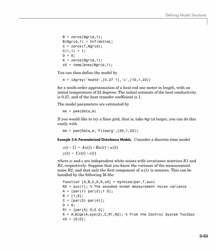
Defining Model Structures
3-53
B = zeros(Ngrid,1); B(Ngrid,1) = htf/deltaL;C = zeros(1,Ngrid);C(1,1) = 1;D = 0;K = zeros(Ngrid,1);x0 = temp ∗ones(Ngrid,1);
You can then define the model by
m = idgrey('heatd',[0.27 1],'c',[10,1,22])
for a tenth-order approximation of a heat rod one meter in length, with an initial temperature of 22 degrees. The initial estimate of the heat conductivity is 0.27, and of the heat transfer coefficient is 1.
The model parameters are estimated by
me = pem(Data,m)
If you would like to try a finer grid, that is, take Ngrid larger, you can do this easily with
me = pem(Data,m,'Filearg',[20,1,22])
Example 3.4: Parameterized Disturbance Models. Consider a discrete-time model
where w and e are independent white noises with covariance matrices R1 and R2, respectively. Suppose that you know the variance of the measurement noise R2, and that only the first component of is nonzero. This can be handled by the following M-file:
function [A,B,C,D,K,x0] = mynoise(par,T,aux)R2 = aux(1); % The assumed known measurement noise varianceA = [par(1) par(2);1 0];B = [1;0];C = [par(3) par(4)];D = 0;R1 = [par(5) 0;0 0];K = A∗ dlqe(A,eye(2),C,R1,R2); % From the Control System Toolboxx0 = [0;0];
x t 1+( ) Ax t( ) Bu t( ) w t( )+ +=y t( ) Cx t( ) e t( )+=
w t( )
3 Tutorial
3-54
State-Space Structures: Initial Values and Numerical DerivativesFor a structured state-space model, it is sometimes difficult to find good initial parameter values at which to start the numerical search for a minimum of (Equation 3-38). It is always best to use physical insight, whenever possible, to suggest such values. For random initialization, the command init is useful. Since there is always a risk that the numerical minimization may get stuck in a local minimum, it is advisable to try several different initialization values for
.
In the search for the minimum, the gradient of the prediction errors with respect to the parameters is computed by numerical differentiation. The step size is determined by the M-file nuderst. In its default version, the step size is simply times the absolute value of the parameter in question (or the number if this is larger). When the model structure contains parameters with different orders of magnitude, try to scale the variables so that the parameters are all roughly the same magnitude. You might need to edit the M-file nuderst to address the problem of suitable step sizes for numerical differentiation.
Estimating Continuous-Time Models: General RemarksIn many cases you want to estimate a continuous-time model. The System Identification Toolbox gives several ways for you to do this:
• Estimate a discrete-time model, and convert it to continuous time by the command d2c. Note that the estimated model contains information about the input intersample properties of the estimation data, and the conversion, by default, will be in accordance with this information. If a polynomial type model (idpoly model) is estimated, the number of numerator and denominator coefficients can be chosen freely for the discrete-time model. Note, however, that the transformed continuous-time model generically has a numerator order that is one less than (or equal to, if nk = 0) the denominator order, regardless of the discrete-time orders.
m = oe(data,[3 4 1]);mc = d2c(m)
θ
e t( )
10 4–
10 7–
Defining Model Structures
3-55
• Use continuous-time frequency-domain data and directly estimate an idpoly continuous-time model. Then the numerator and denominator orders can be chosen freely. In the case below it is assumed that the data is sampled so fast (or that the input is band limited) so that frequencies above the Nyquist frequency in the continuous-time input are negligible.
DF = fft(data)DF.ts = 0 (% treating the frequency data as continuous time)m = oe(DF,[nb nf])
Here nb is the number of numerator coefficients and nf the number of denominator coefficients. The delay order, nk, has no meaning for continuous-time OE models, and should be omitted. This means that for nb = 2, nf = 4 the model is
(3-57)
If the data is sampled fast, it is usually a good idea to apply some low-pass filtering before making the fit. This is most easily done with the focus property.
m = oe(DF,[nb nf],'focus',[0 10])
meaning that only data in the frequency interval between 0 and 10 rad/s is used in the model estimation.
Of course, continuous-time frequency-domain data can also be used to estimate continuous-time state-space models.
m = pem(DF,n)
This will give an nth-order continuous-time state-space model with no direct term (D matrix = 0). To include a D matrix, indicate that “the relative degree” nk is zero.m = pem(DF,n,'nk',0)
• Use continuous-time process models as described in “Process Models: the idproc Model” on page 3-41.m = pem(data,'P1D')
G s( )b1s b2+
s4 f1s3 f2s2 f3s f4+ + + +-----------------------------------------------------------------=
3 Tutorial
3-56
• Build a continuous-time idgrey model as described in “State-Space Models with Coupled Parameters: the idgrey Model” on page 3-51, and in Example 3.3 on page 3-52.
• Build a continuous-time idss model either in structured or in free form as described in “Black-Box State-Space Models: the idss Model” on page 3-46.
In the latter three cases you can directly estimate the continuous-time model from discrete-time data (or continuous-time frequency-domain data) without further information, since the iddata object contains all relevant information to adjust the model to the data.
m = pem(Data,mi)
If you create a state-space model at the same time as you estimate it, you must, however, indicate whether you want to obtain a continuous-time model.
m = n4sid(Data,5,'Ts',0)m = pem(Data,5,'Ts',0,'ss','can')
In the pem example, the ('ss','can') property name/property value pair means that the state-space parameterization ('SSparameterization') is 'Canonical'. Estimation of freely parameterized continuous-time state-space models is not supported.
Examining Models
3-57
Examining ModelsOnce you have estimated a model, you need to investigate its properties. You have to simulate it, test its predictions, and compute its poles and zeros and so on. You thus have to transform the model to various ways of representing and presenting it. This section deals with how this is done. The following topics are covered:
• Parametric models: basic use, accessing properties, simulation, and prediction. Also manipulating channels, in particular the noise input channels.
• Frequency-domain models
• Graphing model properties
• Transformations to other representations
• Transformations between continuous and discrete time
Parametric Models: idmodel and Its Childrenidmodel is an object that the user does not deal with directly. It contains all the common properties of the model objects idarx, idgrey, idpoly, idproc, and idss, which are returned by the different estimation routines.
Basic UseIf you just estimate models from data, the model objects should be transparent. All parametric estimation routines return idmodel results.
m = arx(Data,[2 2 1])
The model m contains all relevant information. Just typing m gives a brief account of the model. present(m) also gives information about the uncertainties of the estimated parameters. get(m) gives a complete list of model properties.
Most of the interesting properties can be directly accessed by subreferencing.
m.am.da
See the property list obtained by get(m), as well as the property lists of idgrey, idarx, idpoly, idproc, and idss in Chapter 4, “Function Reference,” for more details on this.
3 Tutorial
3-58
The characteristics of the model m can be directly examined and displayed by commands like impulse, step, bode, nyquist, and pzmap. The quality of the model is assessed by commands like compare and resid. If you have the Control System Toolbox, typing view(m) gives you access to various display functions. More details about this will be given below.
To extract state-space matrices, transfer function polynomials, etc., you can use these commands:
arxdata, polydata, tfdata, ssdata, zpkdata
To compute the frequency response of the model, you can use idfrd and freqresp.
Simulation and PredictionAny idmodel m can be simulated with
y = sim(m,Data)
where Data is an iddata object with just input channels.
Data = iddata([ ],[u v])
The number of input channels must either be equal to the number of measured input channels in m, in which case a noise-free simulation is obtained, or equal to the sum of the number of input and output channels in m. In the latter case the last input signals (v) are interpreted as white noise. They are then scaled by the NoiseVariance matrix of m and added to the output via the disturbance model
where the matrix L is given from the noise covariance by .
L=chol(m.NoiseVariance)'
The output is returned as an iddata object with just output channels. Here is a typical string of commands.
A = [1 -1.5 0.7];B = [0 1 0.5];m0 = idpoly(A,B,[1 -1 0.2]);u = iddata([],idinput(400,'rbs',[0 0.3]));
y Gu He+=e Lv=
Λ Λ LLT=
Examining Models
3-59
v= iddata([],randn(400,1));y = sim(m0, [u v]);plot(y)
The “inverse model” (Equation 3-38), which computes the prediction errors from given input-output data, is simulated with
e = pe(m,[y u])
To compute the k-step ahead prediction of the output signal based on a model m, the procedure is as follows:
yhat = predict(m,[y u],k)
The predicted value is computed using the information in up to time and information in up to time . The actual way that the information in past outputs is used depends on the disturbance model in m. For example, an output-error model (that is, H = 1 in (Equation 3-10)) maintains that there is no information in past outputs; therefore, predictions and simulations coincide.
predict can evaluate how well a time-series model is capable of predicting future values of the data. In this example y is the original series of monthly sales figures. A model is estimated based on the first half, and then its ability to predict half a year ahead is checked out on the second half of the observations.
plot(y)y1 = y(1:48), y2 = y(49:96)m4 = ar(y1,4)yhat = predict(m4,y2,6)plot(y2,yhat)
The command compare is useful for any comparisons involving sim and predict.
Dealing with Input and Output ChannelsFor multivariable models, you construct submodels containing a subset of inputs and outputs by simple subreferencing. The outputs and input channels can be referenced according to
m(outputs,inputs)
y t t k–( ) u s( )s t= y s( ) s t k–=

3 Tutorial
3-60
Use the colon (:) to denote all channels and the empty matrix ([ ]) to denote no channels. The channels can be referenced by number or by name. For several names, you must use a cell array.
m3 = m('position',{'power','speed'})
or
m3 = m(3,[1 4])
Thus m3 is the model obtained from m by considering the transfer functions from input numbers 1 and 4 (with input names 'power' and 'speed') to output number 3 (with name 'position').
For a single output model m,
m4 = m(inputs)
selects the corresponding input channels, and for a single input model
m5 = m(outputs)
selects the indicated output channels.
Subreferencing is quite useful, for example, when you want a plot of just some channels.
The Noise ChannelsThe estimated models have two kinds of input channels: the measured inputs u and the noise inputs e. For a general linear model m, we have
(3-58)
where u is the nu-dimensional vector of measured input channels and e is the ny-dimensional vector of noise channels. The covariance matrix of e is given by the property 'NoiseVariance'. Occasionally this matrix is written in factored form:
This means that e can be written as
y t( ) G q( )u t( ) H q( )e t( )+=
Λ
Λ LLT=
e Lv=
Examining Models
3-61
where v is white noise with identity covariance matrix (independent noise sources with unit variances).
If m is a time series (nu = 0), G is empty and the model is given by
(3-59)
For the model m in (Equation 3-58), the restriction to the transfer function matrix G is obtained by
m1 = m('measured') or just m1 = m('m')
Then e is set to 0 and H is removed.
Analogously
m2 = m('noise') or just m2 = m('n')
creates a time-series model m2 from m by ignoring the measured input. That is m2 is given by (Equation 3-59).
For a system with measured inputs, bode, step, and many other transformation and display functions just deal with the transfer function matrix G. To obtain or graph the properties of the disturbance model H, it is therefore important to make the transformations m('n'). For example,
bode(m('n'))
will plot the additive noise spectra according to the model m, while
bode(m)
just plots the frequency responses of G.
To study the noise contributions in more detail, it might be useful to convert the noise channels to measured channels, using the command noisecnv.
m3 = noisecnv(m)
This creates a model m3 with all input channels, both measured u and noise sources e, being treated as measured signals. That is, m3 is a model from u and e to y, describing the transfer functions G and H. The information about the variance of the innovations e is then lost. For example, studying the step response from the noise channels does not take into consideration how large the noise contributions actually are.
y t( ) H q( )e t( )=
3 Tutorial
3-62
To include that information, e should first be normalized , so that becomes white noise with an identity covariance matrix.
m4 = noisecnv(m,'Norm')
This creates a model m4 with and treated as measured signals.
For example, the step responses from v to y will now also reflect the typical size of the disturbance influence because of the scaling by L. In both these cases, the previous noise sources that have become regular inputs will automatically get input names that are related to the corresponding output. The unnormalized noise sources e have names like 'e@y1' (noise e at output channel with name y1), while the normalized sources v are called 'v@y1'.
Retrieving Transfer FunctionsThe functions that retrieve transfer function properties, ssdata, tfdata, and zpkdata, will thus work as follows for a model (Equation 3-58) with measured inputs. (fcn is any of ssdata, tfdata, or zpkdata).
fcn(m) returns the properties of G (ny outputs and nu inputs).
fcn(m('n')) returns the properties of the transfer function H (ny outputs and ny inputs).
fcn(noisecnv(m)) returns the properties of the transfer function [G H] (ny outputs and ny+nu inputs).
fcn(noisecnv(m,'Norm')) returns the properties of the transfer function [G HL} (ny outputs and ny+nu inputs. Analogously,
fcn(noisecnv(m('n'),'Norm'))
returns the properties of the transfer function HL (ny outputs and ny inputs).
If m is a time-series model, fcn(m) returns the properties of H, while
fcn(noisecnv(m,'Norm'))
returns the properties of HL.
e Lv= v
u v
y t( ) G q( )u t( ) H q( )Lv t( )+ G HLuv
= =
Examining Models
3-63
Note that the estimated covariance matrix NoiseVariance itself is uncertain. This means that the uncertainty information about H is different from that of HL.
idmodel PropertiesSee the idmodel reference page for a complete list of idmodel properties.
Adding Channelsm = [m1,m2,...,mN]
creates an idmodel object m, consisting of all the input channels in m1,... mN. The output channels of mk must be the same. Analogously,
m = [m1;m2;... ;mN]
creates an idmodel object m consisting of all the output channels in m1, m2,..., mN. The input channels of mk must all be the same.
If you have the Control System Toolbox, interconnections between idmodels, like G1+G2, G1*G2, append(G1,G2), feedback(G1,G2), etc., can be performed just as for LTI objects. However, covariance information is typically lost.
Frequency Function Format: the idfrd ModelFrequency functions and spectra are stored as an idfrd (Identified Frequency Response Data) model object (which is not a child of idmodel). This model format is used by spa,spafdr, and etfe to deliver their results. Moreover, any idmodel can be transformed to an idfrd object.
The frequency function and the disturbance spectrum corresponding to an idmodel m are computed by
h = idfrd(m)
This gives G and in (Equation 3-11) along with their estimated covariances, which are translated from the covariance matrix of the estimated parameters. The frequencies can be specified as in h = idfrd(m,w), but otherwise a default choice of frequencies (based on the dynamics of m) is used. If m corresponds to a continuous-time model, the frequency functions are computed accordingly.
Φˆ
v
3 Tutorial
3-64
The functions are retrieved by h.ResponseData, h.CovarianceData, h.SpectrumData, and h.NoiseCovariance or any case-insensitive abbreviation of the names. The frequency vector is contained in h.Frequency.
In addition, an idfrd model can be defined directly from the frequency functions. See the idfrd reference page, which also contains a list of idfrd properties. The channels of an idfrd model can be manipulated analogously to idmodels.
An alternative is to compute the response functions without storing them as idfrd objects.
[Response,Frequency,Covariance] = freqresp(m)
Graphs of Model PropertiesThere are several commands in the toolbox for graphing model characteristics,.
• bode
• compare
• ffplot
• impulse
• nyquist
• pzmap
• step
They all have the same basic syntax. To look at one model, use
command(Model)
where command is any of the functions listed above.
command(Mod1,Mod2,...,ModN)
shows a comparison of several models. Modk can be any idmodel models. They can be used with any of the Control System Toolbox’s LTI models. For some commands Modk can also be idfrd and iddata objects. For multivariable models, the plots are grouped so that each input/output channel (for all models) is plotted together. The InputName and OutputName properties of the models are used for this. The number of channels need not be the same in the different models, which is quite useful when you are trying to find a good model of a multivariable system.

Examining Models
3-65
command(Mod1,PlotStyle1,...,ModN,PlotStyleN)
allows you to define colors, line styles, and markers associated with the different models. PlotStyle takes values such as 'b' (for blue), 'b:' (for a blue dotted line), or 'b*-' (for a blue solid line with the points marked by a star). This is the same as for the usual plot command.
To show the uncertainty of the model characteristics, use
command(Mod1,...,ModN,'sd',SD)
This will mark, using dash-dotted lines, a confidence region around the nominal model corresponding to SD standard deviations (for the Gaussian distribution). This region is computed using the estimated covariance matrix for the estimated parameters.
command(Mod1,...,ModN,'sd',SD,'fill')
shows the uncertainty region as a filled region instead.
The different commands have some further options to select time or frequency ranges. See the detailed descriptions in Chapter 4, “Function Reference.”
If Model contains measured input channels, the plot shows just the transfer functions from these measured inputs to the outputs, that is, G in (Equation 3-58). To graph the response from the noise sources, use
command(Model('n'))
For the frequency-response graphs, this shows the additive disturbance spectra, that is, the spectra of the signal H(q)e(t) in Equation 3-58, so that the properties of the noise source e are included in the plot.
For the other graphs, the properties of the transfer function H are shown. That is, no noise normalization is done. The same is true if Model is a time series and has no measured input channels. That means that, for example, step shows the step response of the transfer function H, without accounting for the size (covariance matrix) of e. To include such effects, the disturbances should first be converted to normalized noise sources, using the command noisecnv. See “The Noise Channels” on page 3-60.
Model OutputAn important and visually suggestive plot is to compare the measured output signal with the models’ simulated or predicted outputs. This is achieved by
3 Tutorial
3-66
compare(Data,model)
The input signal in Data is used by the model(s) to simulate the output. This simulated output is shown together with the measured output, which reveals what features in the data the model can and cannot reproduce. Also a legend shows the fit between the signals, in terms of how much of the output variation is reproduced by the model(s).
Frequency ResponseThree functions offer graphic display of the frequency functions and spectra: bode, ffplot, and nyquist.
bode(G)
plots the Bode diagram of G (logarithmic scales and frequencies in rad/s). If G is a spectrum, only an amplitude plot (the power spectrum) is given. Here G can be any idmodel or idfrd object.
The command ffplot has the same syntax as bode but works with linear frequency scales and Hertz as the unit. The command nyquist also has the same syntax, but produces Nyquist plots, that is, graphs of the frequency function in the complex plane.
Transient ResponseThe impulse and step responses of the models are shown by
impulse(Model)
and
step(Model)
impulse and step follow the general syntax, but can also accept iddata objects as arguments. For direct estimation of step and impulse responses from data, use the procedure described in “Estimating Impulse Responses” on page 3-15.
Zeros and PolesThe zeros and poles are graphed by
pzmap(Model)
This gives a plot with 'x' marking poles and 'o' marking zeros. Otherwise, pzmap follows the general syntax.

Examining Models
3-67
GeneralIf you have the Control System Toolbox,
view(Model)
opens the LTI viewer with access to a number of model displays. No uncertainty information can be shown, though.
Transformations to Other Model RepresentationsWithin the structure in which the model was created, you can extract parametric information using the get function or by subscripting. For example, for a state-space model, Mod.A is the A matrix, while Mod.dA contains its standard deviations. For a polynomial model, Mod.a and Mod.da are the A polynomial and its standard deviation.
Generally speaking you can transform to another representation by just using the object constructor, as in
modss = idss(Model)modp = idpoly(Model)
Analogously, if you have the Control System Toolbox, you can freely transform between the different idmodel objects and the LTI objects.
syss = ss(Model)systf = tf(Model)Model = idss(Ltisys)
In addition, regardless of the particular model structure, there are a number of commands that compute various model representations. These all have the basic syntax
[G, dG] = command(Model)
where G contains model characteristics and dG their standard deviation or covariance. The transformation commands are
[A,B,C,D,K,X0,dA,dB,dC,dD,dK,dX0] = ssdata(Model)
[a,b,c,d,f,da,db,dc,dd,df] = polydata(Model)
[A,B,dA,dB] =arxdata(Model)
[Num,Den,dNum,dDen] = tfdata(Model)
3 Tutorial
3-68
[Z,P,K,CovZ,CovP,covK] = zpkdata(Model)
G = idfrd(Model)
[H,w,CovH] = freqresp(Model)
The two last commands were described previously. The three first commands clearly transform to the state-space, the polynomial, and the multivariable ARX representations. See “Defining Model Structures” on page 3-39. tfdata and zpkdata compute the transfer functions and zeros, poles and transfer function gains. See Chapter 4, “Function Reference,” for details.
Discrete- and Continuous-Time Models
Continuous-Time ModelsContinuous-time models are created and recognized by the property 'Ts' = 0. All idmodel objects can be created and analyzed as continuous-time models by setting Ts equal to zero at the time of creation, as in
m = idpoly(1,[0 1 1],1,1,[1 2 3],'Ts',0)
for the model
All model characteristics are then computed and graphed for the continuous-time representation. Time and frequency scales are determined based on the dynamics of the system (the pole/zero locations).
For simulation and prediction, the continuous-time models are first converted to discrete time, using the sampling interval and intersample behavior of the data.
Estimating Continuous-Time ModelsThe estimation routines support the estimation of continuous-time state-space models in several different ways. This was described in “Estimating Continuous-Time Models: General Remarks” on page 3-54.
The major reason for identifying continuous-time models is to secure a particular structure of the continuous-time state-space matrices. This would typically reflect a physical interpretation or some gray-box modeling work
y s 1+
s2 2s 3+ +----------------------------u e+=
Examining Models
3-69
done, as for the process models, described in “Process Models: the idproc Model” on page 3-41, or continuous-time idss or idgrey models, as described in “Black-Box State-Space Models: the idss Model” on page 3-46.
TransformationsTransformations between continuous-time and discrete-time model representations are achieved by c2d and d2c. Note that it is not sufficient just to assign a new value of Ts to the model object. The corresponding uncertainty measure (the estimated covariance matrix of the internal parameters) is also transformed in most cases. The syntax is
modc = d2c(modd)modd = c2d(mc,T)
If the discrete-time model has some pure time delays ( ), the default command removes them before forming the continuous-time model, and appends them using the property InputDelay in model modc. This property is used to add appropriate phase lag and shift the data whenever the model is used. d2c also offers an option to approximate the dead time by a finite dimensional system. Note that the disturbance properties are translated by the somewhat questionable formula (Equation 3-29). The covariance matrix is translated by the Gauss approximation formula using numerical derivatives. The M-file nuderst is then invoked. You might want to edit it for applications where the parameters have very different orders of magnitude. See the comments in “State-Space Structures: Initial Values and Numerical Derivatives” on page 3-54.
Here is an example that compares the Bode plots of an estimated model and its continuous-time counterpart.
m= armax(Data,[2 3 1 2]);mc = d2c(m); bode(m,mc)
The transformations between discrete and continuous time depend on the intersample behavior of the input. The formulas are different if the input is assumed to be piecewise constant or piecewise linear between samples ('zoh' or 'foh'). For estimated discrete-time models, the input properties of the estimation data are used for this purpose, by default. To override this, add an extra argument, as described in the reference pages for c2d and d2c.
nk 1>
3 Tutorial
3-70
Model Structure Selection and Validation After you have been analyzing data for some time, you typically end up with a large collection of models with different orders and structures. You need to decide which one is best, and if the best description is an adequate model for your purposes. These are the problems of model validation.
Model validation is the heart of the identification problem, but there is no absolute procedure for approaching it. It is wise to be equipped with a variety of different tools with which to evaluate model qualities. The command advice can be applied to any estimated model for some hints on the model’s quality.
advice(Model)
This section describes the techniques you can use to evaluate model qualities using the System Identification Toolbox.
Comparing Different StructuresIt is natural to compare the results obtained from model structures with different orders. For state-space models, you can easily obtain this by using a vector argument for the order in n4sid or pem.
m = n4sid(Data,1:10)m = pem(Data,'nx',3:15)
This invokes a plot from which a “best” order is chosen. Just omitting the order argument, m = n4sid(Data) or pem(Data) makes a default choice of the best order.
For models of ARX type, various orders and delays can be efficiently studied with the command arxstruc. Collect in a matrix NN all of the ARX structures you want to investigate, so that each row of NN is of the type
[na nb nk]
With
V = arxstruc(Date,Datv,NN)
an ARX model is fitted to the data set Date for each of the structures in NN. Next, for each of these models, the sum of squared prediction errors is computed as they are applied to the data set Datv. The resulting loss functions are stored in V together with the corresponding structures.
Model Structure Selection and Validation
3-71
To select the structure that has the smallest loss function for the validation set Datv, use
nn = selstruc(V,0)
Such a procedure is known as cross validation and is a good way to approach the model selection problem.
It is usually a good idea to visually inspect how the fit changes with the number of estimated parameters. A graph of the fit versus the number of parameters is obtained with
selstruc(V)
This routine prompts you to choose the number of parameters to estimate, based upon visual inspection of the graph. Then it selects the structure with the best fit for that number of parameters.
The command struc helps generate typical structure matrices NN for single-input systems. A typical sequence of commands is
V = arxstruc(Date,Datv,struc(2,2,1:10));nn = selstruc(V,0);nk = nn(3);V = arxstruc(Date,Datv,struc(1:5,1:5,nk-1:nk+1));selstruc(V)
where you first establish a suitable value of the delay nk by testing second-order models with delays between one and ten. The best fit selects the delay, and then all combinations of ARX models with up to five a and b parameters are tested with delays around the chosen value (a total of 75 models).
If the model is validated on the same data set from which it was estimated, that is, if Date = Datv, the fit always improves as the flexibility of the model structure increases. You need to compensate for this automatic decrease of the loss functions. There are several approaches for this. Probably the best known technique is Akaike’s Final Prediction Error (FPE) criterion and his closely related Information Theoretic Criterion (AIC). Both simulate the cross validation situation, where the model is tested on another data set.
3 Tutorial
3-72
The FPE is formed as
where d is the total number of estimated parameters and N is the length of the data record. V is the loss function (quadratic fit) for the structure in question. The AIC is formed as
(See Section 16.4 in Ljung (1999).)
According to Akaike’s theory, in a collection of different models, choose the one with the smallest FPE (or AIC). You can display the FPE values with the model parameters by just typing the model name. It is also one of the fields in EstimationInfo and can be accessed by
FPE = fpe(m)
Similarly, the AIC value of an estimated model is obtained as
AIC = aic(m)
The structure that minimizes the AIC is obtained with
nn = selstruc(V,'AIC')
where V was generated by arxstruc.
A related criterion is Rissanen’s Minimum Description Length (MDL) approach, which selects the structure that allows the shortest overall description of the observed data. This is obtained with
nn = selstruc(V,'MDL')
If substantial noise is present, the ARX models might need to be of high order to describe simultaneously the noise characteristics and the system dynamics. (For ARX models the disturbance model 1/A(q) is directly coupled to the dynamics model B(q)/A(q).)
FPE1 d
N----+
1 dN----–
--------------V=
AIC V 1 2 dN----+
log=
Model Structure Selection and Validation
3-73
Impulse Response to Determine DelaysThe command impulse applied to a data set
impulse(Data,'sd',3)
shows a nonparametric estimate of the impulse response. In the call above, a confidence region around zero is also shown, corresponding to three standard deviations (ca 99.9%). Any part of the impulse response that is outside this region is thus significant. The first sample after t = 0, at which the impulse response estimate crosses the confidence band, is thus a good estimate of the delay in the channel in question.
Significant impulse response estimates for negative time lags are indications of feedback in the data.
Checking Pole-Zero CancellationsA near pole-zero cancellation in the dynamics model is an indication that the model order might be too high. To judge whether a “near” cancellation is a real cancellation, take the uncertainties in the pole and zero locations into consideration
pzmap(mod,'sd',1)
where the 1 indicates how many standard deviations wide the confidence interval is. If the confidence regions of a zero and a pole overlap, try lower model orders.
This check is especially useful when the models have been generated by arx. As mentioned previously, the orders can be pushed up because of the requirement that c/A(q) describe the disturbance characteristics. Checking cancellations in B(q)/A(q) then gives a good indication of which orders to choose from model structures like armax, oe, and bj.
Residual AnalysisThe residuals associated with the data and a given model, as in (Equation 3-38), are ideally white and independent of the input for the model to correctly describe the system. The function
resid(Model,Data)
3 Tutorial
3-74
computes the residuals (prediction errors) e from the model when applied to Data, and performs whiteness and independence analyses. The autocorrelation function of e and the cross-correlation function between e and u are computed and displayed for up to lag 25. Also displayed are 99% confidence intervals for these variables, assuming that e is indeed white and independent of u.
The rule is that if the correlation functions go significantly outside these confidence intervals, do not accept the corresponding model as a good description of the system. Some qualifications of this statement are necessary:
• Model structures like the OE structure (Equation 3-17) and methods like the IV method (Equation 3-41) focus on the dynamics G and less about the disturbance properties H. If you are interested primarily in G, focus on the independence of e and u rather than the whiteness of e.
• Correlation between e and u for negative lags, or current affecting future , is an indication of output feedback. This is not a reason to reject the model. Correlation at negative lags is of interest, because certain methods do not work well when feedback is present in the input-output data (see “Feedback in Data” on page 3-83), but concentrate on the positive lags in the cross-correlation plot for model validation purposes.
• When you are using the ARX model (Equation 3-14), the least squares procedure automatically makes the correlation between and zero for , , , for the data used for the estimation.
The residuals e together with the input u are returned by
E = resid(Model,Data)
as an iddata object. As part of the validation process, you can graph the residuals using
plot(E)
for a simple visual inspection of irregularities and outliers. (See also “Outliers and Bad Data; Multiple-Experiment Data” on page 3-81.)
Model Error ModelsThe residual call
E = resid(Model,Data)
e t( )u t( )
e t( ) u t k–( )k nk= nk 1+ …nk nb 1–+
Model Structure Selection and Validation
3-75
returns the iddata object e, which has the inputs in Data as inputs and the prediction errors (residuals) as outputs. Building models using e will thus reveal if there is any significant influence from u to e left in the data. Such models are called Model Error Models, and examining them is a good complement to traditional residual analysis.
E= resid(Model,Data)impulse(E,'sd',3) % An alternative to residual analysisbode(spa(E),'sd',3) % Shows the frequency ranges
% with significant model errorsm = arx(E,[0 10 0])bode(m,'sd',3)
Note that the resid command has several options to display model error properties rather than correlation functions.
Noise-Free SimulationsTo check whether a model is capable of reproducing the observed output when driven by the actual input, you can run a simulation.
u = Data(:,[],:) % Extracting the input from the datayh = sim(Model,u)y = Data(:,:,[]) % Extracting the output from the dataplot(y,yh)
The same result is obtained by
compare(Data,Model)
It is a much tougher and more revealing test to perform this simulation, as well as the residual tests, on a fresh data set Data that was not used for the estimation of the model Model. This is called cross validation.
Assessing the Model UncertaintyThe estimated model is always uncertain, due to disturbances in the observed data and the lack of an absolutely correct model structure. The variability of the model that is due to the random disturbances in the output is estimated by most of the estimation procedures, and it can be displayed and illuminated in a number of ways. This variability answers the question of how different can the model be if the identification procedure is repeated, using the same model structure, but with a different data set that uses the same input sequence. It
3 Tutorial
3-76
does not account for systematic errors due to an inadequate choice of model structure. There is no guarantee that the “true system” lies in the confidence interval. The rule is that the model should pass a residual analysis (see “Residual Analysis” on page 3-73) test (correlation functions essentially inside the confidence lines) for the uncertainty bounds to be regarded as reliable.
The uncertainty in the different model views is displayed if the argument 'sd' is included in the argument list,
command(Model,'sd',sd)
as explained in “Graphs of Model Properties” on page 3-64.
The uncertainty in the time response is displayed by
simsd(Model,u)
Ten possible models are drawn from the asymptotic distribution of the model Model. The response of each of them to the input u is graphed on the same diagram.
The uncertainty of these responses concerns the external input-output properties of the model. It reflects the effects of inadequate excitation and the presence of disturbances.
You can also directly get the standard deviation of the simulated result by
[ysim,ysimsd] = sim(Model,u)
The uncertainty in internal representations is manifested in the covariance matrix of the estimated parameters
Model.CovarianceMatrix
which is used to give the standard deviations of all model characteristics. The parametric uncertainty is directly available as
Model.da
for the standard deviations of Model.a.
Note that state-space models, estimated in a free parameterization, do not have well-defined standard deviations of the matrix elements. The model still has stored the uncertainty of the input-output behavior, so other model representations and graphs will show the uncertainty. For a state-space model
Model Structure Selection and Validation
3-77
in a free parameterization, it is possible to first transform it to a canonical parameterization and then display the matrix parameter uncertainties.
Model = pem(Data,5)Modelc = ModelModelc.ss = 'canon'Modelc.da
All routines for computing and displaying model characteristics also offer to calculate and show the uncertainties. See “Transformations to Other Model Representations” on page 3-67.
Large uncertainties in these representations are caused by excessively high model orders, inadequate excitation, or bad signal-to-noise ratios.
Comparing Different ModelsIt is a good idea to display the model properties in terms of quantities that have more physical meaning than the parameters themselves. Bode plots, pole-zero plots, and model simulations all give a sense of the properties of the system that have been picked up by the model.
If several models of different characters give very similar Bode plots in the frequency range of interest, you can be fairly confident that these must reflect features of the true, unknown system. You can then choose the simplest model among these.
A typical identification session includes estimation in several different structures, and comparisons of the model properties. Here is an example.
a1 = arx(Data,[1 2 1]);g = spa(Data);bode(g,a1)bode(g('n'),a1('n'))% the output disturbance spectraam2 = armax(Data,[2 2 2 1]);bode(g,am2)pzmap(a1,am2,'sd',3)
Selecting Model Structures for Multivariable SystemsA multivariable (MIMO) system is a system with several input and output channels. All model structures in the toolbox support models with one output
3 Tutorial
3-78
and several inputs. Polynomial models, idpoly, do not handle multioutput models, however.
Model StructuresMultivariable systems offer a potentially richer internal structure. The easiest approach, in the black-box situation, is to think just in terms of input delays and state-space model order.
A recommended approach is to get an idea of input delays from the nonparametric impulse response estimate and determine the vector nk = [nk1,nk2,...,nkm] where nkj is the minimal delay from input j to any of the output channels. Then try state-space models with several orders and with these delays.
impulse(Data,'sd',3)Model = n4sid(Data(1:500),'nx',1:10,'nk',nk)compare(Data(501:1000),Model)
The compare plot will reveal which output channels are easy and which are difficult to reproduce.
An alternative to find the delays is to first estimate a parametric model with delays 1, and then examine the impulse responses of this model and determine the delays.
Model = pem(Data) % This uses 'best' model order.impulse(Model,'sd',3)Model = pem(Data,'nx',1:10,'nk',nk)
To test models with delay 0 in a similar way, use
Model = pem(Data,'best','nk',zeros(size(nk)))
Significant responses at delay 0 must be examined with care, because they might be caused by feedback.
Note that delays nk larger than 1 will be incorporated in the model structure, and thus increase the state-space model order from the nominal one with sum(max(nk-1,zeros(size(nk)))). An alternative is to use the property 'InputDelay'. This leads to a model that has the same delays as for 'nk'. These are not explicitly shown in the model matrices, but stored as a property to be used when necessary. See “nk and InputDelay” on page 3-101. See also the properties of idss on the reference page.

Model Structure Selection and Validation
3-79
If you have detailed knowledge about which orders and delays are reasonable in the different input/output channels, you can use multivariable ARX models in the idarx model format. This allows you to define the orders of the input and output lags, as well as the delays, independently for the different channels.
Black-box parameterizations of multivariable systems require many parameters. Therefore, it might be important to incorporate any essential structure knowledge based on physical insight. You typically do this with continuous-time, custom model parameterizations using structured idss or idgrey models. See “Structured State-Space Models with Free Parameters: the idss Model” on page 3-48 and “State-Space Models with Coupled Parameters: the idgrey Model” on page 3-51.
Channel SelectionA particular aspect of multivariable models is the selection of channels. Models for subselections of input-output channels can be quite useful and informative. Generally speaking the models become “better” when more input channels are used, and “worse” when more output channels are used. The latter observation is due to the fact that such models have “more to explain.”
If you build models with several outputs and find, using compare, a certain output channel to be difficult to reproduce, then try to build a model of this channel alone. This will reveal if there are inherent difficulties with this output, or if it is just too difficult to handle it together with other outputs.
Analogously, if you see that using, for example, step or impulse, a certain input channel seems to have an insignificant influence on the outputs, then remove that channel, and examine whether the corresponding model becomes any worse, for example, in the compare plots.
The toolbox’s data and model objects give full support for the bookkeeping required for these channel subselections. You select channels by direct subreferencing, and the InputName and OutputName properties form the basis for a correct combination of channels. The subreferencing follows:
Data(Samples,Outputs,Inputs)Model(Outputs,Inputs)
3 Tutorial
3-80
Typical command sequences can be
Date = Data(1:500)Datv = Data(501:1000)m = pem(Date)compare(Datv,m)m1 = pem(Date(:,3,4))compare(Datv,m,m1)bode(m,m1)compare(Datv,m(:,4),m1)
Dealing with Data
3-81
Dealing with DataExtracting information from data is not an entirely straightforward task. In addition to the decisions required for model structure selection and validation, the data might need to be handled carefully. This section gives some advice on handling several common situations.
Offset LevelsWhen the data has been collected from a physical plant, it is typically measured in physical units. The levels in these raw input and output measurements might not match in any consistent way. This will force the models to waste some parameters correcting the levels.
Typically, linearized models are sought around some physical equilibrium. In such cases offsets are easily dealt with: subtract the mean levels from the input and output sequences before the estimation. It is best if the mean levels correspond to the physical equilibrium, but if such values are not known, use the sample means.
Data = detrend(Data);
Section 14.1 in Ljung (1999) discusses this in more detail. There are situations when it is not advisable to remove the sample means. It could be, for example, that the physical levels are built into the underlying model, or that integrations in the system must be handled with the right level of the input being integrated.
With the detrend command, you can also remove piecewise linear trends.
Outliers and Bad Data; Multiple-Experiment DataReal data are also subject to possible bad disturbances: an unusually large disturbance, a temporary sensor or transmitter failure, etc. It is important that such outliers are not allowed to affect the models too strongly.
The robustification of the error criterion (described under LimitError in Algorithm Properties on page 4-14) helps here, but it is always good practice to examine the residuals for unusually large values, and to go back and critically evaluate the original data responsible for the large values. If the raw data are obviously in error, they can be smoothed and the estimation procedure repeated.
3 Tutorial
3-82
Often the data has portions with bad behavior. This can, for example, be due to big disturbances or sensor failures over a period of time. It can also be that there are time periods where “nothing happens,” the input is not exciting, etc. Then the best alternative is to break up the data into pieces of informative portions. By merging the pieces into a multiple-experiment iddata object, they can still be used together to build models. Another situation when multiple-experiment data is useful is when several different experiments have been performed on the same plant. The estimation routines take proper action to handle the different pieces. All estimation, simulation, and validation routines in the toolbox handle multiple-experiment data in a transparent fashion. A typical string of commands could be
plot(Data)Datam = merge(Data(1:340),Data(500:897), ...
Data(1001:1200),Data(1550:2000))m =pem(getexp(Datam[1,2,4])) % Portions 1,2 and 4 for estimationcompare(getexp(Datam,3),m) % Portion 3 for validation
Missing DataIn practice it is often the case that certain measurement samples are missing. The reason might be sensor failures or data acquisition failures. It may be that the data are directly reported as missing, or that plots reveal that some values are obviously in error. This can apply both to inputs and outputs. In these cases, replace the missing data by NaN when forming the signal matrices and the iddata object. The routine misdata can then be applied to reconstruct the missing data in a reasonable way.
dat = iddata(y,u,0.2) % y and/or u contain NaN for missing data.dat1 = misdata(dat);plot(dat,dat1) % Checking how the missing data
% have been estimated in dat1m = pem(dat1) % Model estimated using reconstructed missing data
See Section 14.2 in Ljung (1999) for a discussion on missing data.
Filtering Data: FocusDepending upon the application, interest in the model can be focused on specific frequency bands. Filtering the data before the estimation, through filters that enhance these bands, improves the fit in the interesting regions.
Dealing with Data
3-83
This is accomplished in the System Identification Toolbox by the property 'Focus'. For example, to enhance the fit in the frequency band between 0.05 and 1 rad/s, execute one of the following:
m = pem(Data,3,'Foc',[0.05 1])ma = arx(Data,[2 3 1],'Foc',[0.05 1])
This computes and uses a fifth-order Butterworth bandpass filter with passband between the indicated frequencies. The data is filtered through this filter before fitting the transfer function from the measured inputs (G in (Equation 3-58)) to the outputs. The disturbance model (H) is, however, estimated using the unfiltered data. Chapter 14 in Ljung (1999) discusses the role of filtering in more detail.
For a model that does not use a disturbance description (that is, H = 1 in (Equation 3-58), which corresponds to K = 0 for state-space, and na = nc = nd = 0 for polynomial models), the Focus effect is the same as applying the routine to filtered data. That is,
m = pem(Data,3,'Foc',[0.05 1],'dist','none')Df = idfilt(Data,[0.05 1]);m = pem(Df,3,'dist','none')
give the same model.
The System Identification Toolbox contains other useful commands for related problems. For example, if you want to lower the sampling rate by a factor of 5, use
Dat5 = resample(Data,1,5);
Feedback in DataIf the system was operating in closed loop (feedback from the past outputs to the current input) when the data were collected, some care has to be exercised.
Basically, all the prediction error methods work equally well for closed-loop data. Note, however, that the output-error model (Equation 3-17) and the Box-Jenkins model (Equation 3-18) are normally capable of giving a correct description of the dynamics G, even if H (which equals 1 for the output-error model) does not allow a correct description of the disturbance properties. This is no longer true for closed-loop data. You then need to model the disturbance properties more carefully. Another thing to be cautious about is that impulse

3 Tutorial
3-84
response effects at delay 0 very well could be traced to the feedback mechanism and not to the system itself.
The spectral analysis method and the instrumental variable techniques (with default instruments) as well as n4sid can give unreliable results when applied to closed-loop data. Avoid these techniques when feedback is present.
To detect whether feedback is present, use the basic method of applying impulse to estimate the impulse response. Significant values of the impulse response at negative lags is a clear indication of feedback. There is also a command, feedback, that can be applied to the data for direct tests.
When a parametric model has been estimated and the resid command is applied, a graph of the correlation between residuals and inputs is given. Significant correlation at negative lags again indicates output feedback in the generation of the input. Testing for feedback is, therefore, a natural part of model validation.
The advice function applied both to data and to estimated models will also comment on possible feedback effects in the data. See the reference page for feedback.
DelaysThe selection of the delay nk in the model structure is a very important step in obtaining good identification results. You can get an idea about the delays in the system by the impulse response estimate from impulse.
Incorrect delays are also visible in parametric models. Underestimated delays (nk too small) show up as small values of leading estimates compared to their standard deviations. Overestimated delays (nk too large) are usually visible as a significant correlation between the residuals and the input at the lags corresponding to the missing terms in the resid plot.
A good procedure is to start by using arxstruc to test all feasible delays together with a second-order model. Use the delay that gives the best fit for further modeling. When you have found an otherwise satisfactory structure, vary nk around the nominal value within the structure and evaluate the results.
The command delayest directly estimates the delay, based on the arxstruc command.
bk
bk
Recursive Parameter Estimation
3-85
Recursive Parameter EstimationIn many cases it might be necessary to estimate a model on line at the same time as the input-output data is received. You might need the model to make some decision on line, as in adaptive control, adaptive filtering, or adaptive prediction. It might be necessary to investigate possible time variation in the system’s (or signal’s) properties during the collection of data. Terms like recursive identification, adaptive parameter estimation, sequential estimation, and online algorithms are used for such algorithms. Chapter 11 in Ljung (1999) deals with such algorithms in some detail.
The Basic AlgorithmA typical recursive identification algorithm is
(3-60)
Here is the parameter estimate at time t, and is the observed output at time t. Moreover, is a prediction of the value based on observations up to time and also based on the current model (and possibly also earlier ones) at time . The gain determines in what way the current prediction error affects the update of the parameter estimate. It is typically chosen as
(3-61)
where is (an approximation of) the gradient with respect to of . The latter symbol is the prediction of according to the model described by
. Note that model structures like AR and ARX that correspond to linear regressions can be written as
(3-62)
where the regression vector contains old values of observed inputs and outputs, and represents the true description of the system. Moreover,
is the noise source (the innovations). Compare with (Equation 3-14). The natural prediction is and its gradient with respect to becomes exactly .
For models that cannot be written as linear regressions, you cannot recursively compute the exact prediction and its gradient for the current estimate .
θ t( ) θ t 1–( ) K t( ) y t( ) y t( )–( )+=
θ t( ) y t( )y t( ) y t( )
t 1–t 1– K t( )
y t( ) y t( )–
K t( ) Q t( )ψ t( )=
ψ t( ) θ y t θ( )y t( )
θ
y t( ) ψT t( )θ0 t( ) e t( )+=
ψ t( )θ0 t( )
e t( )y t( ) ψT t( )θ t 1–( )= θ
ψ t( )
θ t 1–( )
3 Tutorial
3-86
Then approximations and must be used instead. Section 11.4 in Ljung (1999) describes suitable ways of computing such approximations for general model structures.
The matrix , which affects both the adaptation gain and the direction in which the updates are made, can be chosen in several different ways. This is discussed in the following.
Choosing an Adaptation Mechanism and GainThe most logical approach to the adaptation problem is to assume a certain model for how the “true” parameters change. A typical choice is to describe these parameters as a random walk.
(3-63)
Here is assumed to be white Gaussian noise with covariance matrix
(3-64)
Suppose that the underlying description of the observations is a linear regression (Equation 3-62). An optimal choice of in (Equation 3-60) and (Equation 3-61) can then be computed from the Kalman filter, and the complete algorithm becomes
(3-65)
Here is the variance of the innovations in (Equation 3-62): (a scalar). The algorithm (Equation 3-65) will be called the
Kalman filter (KF) approach to adaptation, with drift matrix . See Equations (11.66) and (11.67) in Ljung (1999). The algorithm is entirely specified by , , , , and the sequence of data , , , 2, .
y t( ) ψ t( )
Q t( )
θ0
θ0 t( ) θ0 t 1–( ) w t( )+=
w t( )
Ew t( )wT t( ) R1=
Q t( )
θ t( ) θ t 1–( ) K t( ) y t( ) y t( )–( )+=
y t( ) ψT t( )θ t 1–( )=K t( ) Q t( )ψ t( )=
Q t( ) P t 1–( )
R2 ψ t( )TP t 1–( )ψ t( )+-------------------------------------------------------------=
P t( ) P t 1–( ) R1P t 1–( )ψ t( )ψ t( )TP t 1–( )
R2 ψ t( )TP t 1–( )ψ t( )+--------------------------------------------------------------------–+=
R2 e t( )R2 Ee2 t( )=
R1
R1 R2 P 0( ) θ 0( ) y t( ) ψ t( ) t 1=
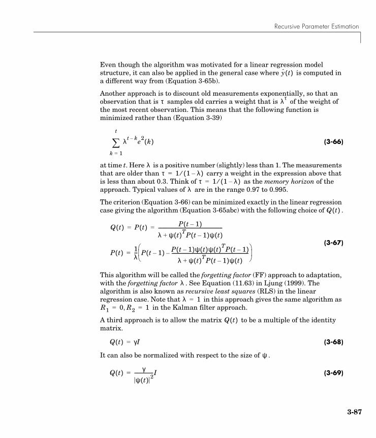
Recursive Parameter Estimation
3-87
Even though the algorithm was motivated for a linear regression model structure, it can also be applied in the general case where is computed in a different way from (Equation 3-65b).
Another approach is to discount old measurements exponentially, so that an observation that is samples old carries a weight that is of the weight of the most recent observation. This means that the following function is minimized rather than (Equation 3-39)
(3-66)
at time t. Here is a positive number (slightly) less than 1. The measurements that are older than carry a weight in the expression above that is less than about 0.3. Think of as the memory horizon of the approach. Typical values of are in the range 0.97 to 0.995.
The criterion (Equation 3-66) can be minimized exactly in the linear regression case giving the algorithm (Equation 3-65abc) with the following choice of .
(3-67)
This algorithm will be called the forgetting factor (FF) approach to adaptation, with the forgetting factor . See Equation (11.63) in Ljung (1999). The algorithm is also known as recursive least squares (RLS) in the linear regression case. Note that in this approach gives the same algorithm as
in the Kalman filter approach.
A third approach is to allow the matrix to be a multiple of the identity matrix.
(3-68)
It can also be normalized with respect to the size of .
(3-69)
y t( )
τ λ τ
λ t k– e2 k( )
k 1=
t
∑
λτ 1 1 λ–( )⁄=
τ 1 1 λ–( )⁄=λ
Q t( )
Q t( ) P t( ) P t 1–( )
λ ψ t( )TP t 1–( )ψ t( )+---------------------------------------------------------= =
P t( ) 1λ--- P t 1–( ) P t 1–( )ψ t( )ψ t( )TP t 1–( )
λ ψ t( )TP t 1–( )ψ t( )+--------------------------------------------------------------------–
=
λ
λ 1=R1 0 R2, 1= =
Q t( )
Q t( ) γI=
ψ
Q t( ) γ
ψ t( ) 2-----------------I=
3 Tutorial
3-88
See Equations (11.45) and (11.46), respectively in Ljung (1999). These choices of move the updates of in (Equation 3-60) in the negative gradient direction (with respect to ) of the criterion (Equation 3-39). Therefore, (Equation 3-68) will be called the unnormalized gradient (UG) approach and (Equation 3-69) the normalized gradient (NG) approach to adaptation, with gain . The gradient methods are also known as least mean squares (LMS) in the linear regression case.
Available AlgorithmsThe System Identification Toolbox provides the following functions that implement all common recursive identification algorithms for model structures in the family (Equation 3-43): rarmax, rarx, rbj, rpem, rplr, and roe. They all share the following basic syntax.
[thm,yh] = rfcn(z,nn,adm,adg)
Here z contains the output-input data as usual. nn specifies the model structure, exactly as for the corresponding offline algorithm. The arguments adm and adg select the adaptation mechanism and adaptation gain listed above.
adm = 'ff'; adg = lam
gives the forgetting factor algorithm (Equation 3-67), with forgetting factor lam.
adm = 'ug'; adg = gam
gives the unnormalized gradient approach (Equation 3-68) with gain gam. Similarly,
adm = 'ng'; adg = gam
gives the normalized gradient approach (Equation 3-69). To obtain the Kalman filter approach (Equation 3-65) with drift matrix R1, enter
adm = 'kf'; adg = R1
The value of is always 1. Note that the estimates in (Equation 3-65) are not affected if all the matrices and are scaled by the same number. You can therefore always scale the original problem so that becomes 1.
The output argument thm is a matrix that contains the current models at the different samples. Row k of thm contains the model parameters, in alphabetical
Q t( ) θθ
γ
R2 θR1 R2, P 0( )
R2
Recursive Parameter Estimation
3-89
order at sample time k, corresponding to row k in the data matrix z. The ordering of the parameters is the same as m.par would give when applied to a corresponding offline model.
The output argument yh is a column vector that contains, in row k, the predicted value of , based on past observations and current model. The vector yh thus contains the adaptive predictions of the outputs, and is useful also for noise canceling and other adaptive filtering applications.
The functions also have optional input arguments that allow the specification of , and . Optional output arguments include the last value of the matrix P and of the vector .
Now, rarx is a recursive variant of arx; similarly rarmax is the recursive counterpart of armax, and so on. Note, though, that rarx does not handle multioutput systems, and rpem does not handle state-space structures.
The function rplr is a variant of rpem, and uses a different approximation of the gradient . It is known as the recursive pseudolinear regression approach, and contains some well-known special cases. See Equation (11.57) in Ljung (1999). When applied to the output-error model (nn=[0 nb 0 0 nf nk]) it results in methods known as HARF ('ff'-case) and SHARF ('ng'-case). The common extended least squares (ELS) method is an rplr algorithm for the ARMAX model (nn=[na nb nc 0 0 nk]).
The following example shows a second-order output-error model, which is built recursively and its time-varying parameter estimates plotted as functions of time.
thm = roe(z,[2 2 1],'ff',0.98);plot(thm)
The next example shows how a second-order ARMAX model is recursively estimated by the ELS method, using Kalman filter adaptation. The resulting static gains of the estimated models are then plotted as a function of time.
[N,dum]=size(z);thm = rplr(z,[2 2 2 0 0 1],'kf',0.01∗ eye(6));nums = sum(thm(:,3:4)')';dens = ones(N,1)+sum(thm(:,1:2)')';stg = nums./dens;plot(stg)
y k( )
θ 0( ) P 0( ), ψ 0( )ψ
ψ
3 Tutorial
3-90
So far, the examples of applications where a batch of data is examined cover studies of the variability of the system. The algorithms are, however, also prepared for true online applications, where the computed model is used for some online decision. You do this by storing the update information in
and information about past data in (and ) and using that information as initial data for the next time step. The following example shows the recursive least squares algorithm being used on line (just to plot one current parameter estimate).
% Initialization, first i/o pair y,u (scalars)[th,yh,P,phi] = rarx([y u],[2 2 1],'ff',0.98);axis([1 50 -2 2])plot(1,th(1),'∗ '),hold%The online loop:for k = 2:50% At time k receive y,u[th,yh,P,phi] = rarx([y u],[2 2 1],'ff',0.98,th',P,phi);plot(k,th(1),'∗ ')end
Execute iddemo #10 to illustrate the recursive algorithms.
Segmentation of DataSometimes the system or signal exhibits abrupt changes during the time when the data is collected. It might be important in certain applications to find the time instants when the changes occur and to develop models for the different segments during which the system does not change. This is the segmentation problem. Fault detection in systems and detection of trend breaks in time series can serve as two examples of typical problems.
The System Identification Toolbox offers the function segment to deal with the segmentation problem. The basic syntax is
thm = segment(z,nn)
with a format like rarx or rarmax. The matrix thm contains the piecewise constant models in the same format as for the algorithms described earlier in this section.
The algorithm that is implemented in segment is based on a model description like (Equation 3-63), where the change term is zero most of the time, but
θ t 1–( ) P t 1–( ), φ t 1–( ) ψ t 1–( )
w t( )

Recursive Parameter Estimation
3-91
now and then it abruptly changes the system parameters . Several Kalman filters that estimate these parameters are run in parallel, each of them corresponding to a particular assumption about when the system actually changed. The relative reliability of these assumed system behaviors is constantly judged, and unlikely hypotheses are replaced by new ones. Optional arguments allow the specification of the measurement noise variance in (Equation 3-62), the probability of a jump, the number of parallel models in use, and also the guaranteed lifespan of each hypothesis. See the segment reference page.
θ0 t( )
R2
3 Tutorial
3-92
Some Special TopicsThis section describes a number of miscellaneous topics. Most of the information here is also covered in other parts of the manual, but since manuals seldom are read from the beginning, you can also check whether a particular topic is brought up here.
Time-Series ModelingWhen there is no input present, the general model (Equation 3-43) reduces to the ARMA model structure.
With you have an AR model structure.
Similarly, a state-space model for a time series is given by
so that the matrices B and D are empty.
Basically all commands still apply to these time-series models, but with natural modifications. They are listed as follows:
m= idpoly(A,[ ],C)e = iddata([],idinput(300,'rgs'))y = sim(m,e)
If a time series s is given as a vector or a matrix, it is put into the iddata format by
y = iddata(s,[],Ts);
Spectral analysis (etfe and spa) returns results in the idfrd model format, which now just contains SpectrumData and its variance. bode will only plot these signal spectra and, if required, the confidence intervals.
g = spa(y)p= etfe(y)bode(g,p,'sd',3)
Note that etfe gives the periodogram estimate p of the spectrum.
A q( )y t( ) C q( )e t( )=
C q( ) 1=
x t 1+( ) Ax t( ) Ke t( )+=y t( ) Cx t( ) e t( )+=
Some Special Topics
3-93
armax and arx work the same way, but need no specification of nb and nk.
th = arx(y,na)th = armax(y,[na nc])
Note that arx also handles multivariable signals, and so do n4sid and pem.
m = n4sid(y) % default orderbode(m)compare(y,m,10) % 10-step ahead predictions being evaluated.
You can build structured state-space models of time series simply by specifying B = [], D = [] in idss and idgrey. resid works the same way for time-series models, but does not provide any input-residual correlation plots.
resid(m,y)
In addition there are two commands that are specifically constructed for building scalar AR models of time series. One is
m = ar(y,na)
which has an option that allows you to choose the algorithm from a group of several popular techniques for computing the least squares AR model. Among these are Burg’s method, a geometric lattice method, the Yule-Walker approach, and a modified covariance method. See Chapter 4, “Function Reference,” for details. The other command is
m = ivar(y,na)
which uses an instrumental variables technique to compute the AR part of a time series.
Finally, when no input is present, the functions bj, iv, iv4, and oe are not of interest.
Here is an example where you can simulate a time series, compare spectral estimates and covariance function estimates, and also the predictions of the model.
ts0 = idpoly([1 -1.5 0.7],[]);ir = sim(ts0,[1;zeros(24,1)]);Ry0 = conv(ir,ir(25:-1:1)); % The true covariance functione = idinput(200,'rgs');y = sim(ts0,e); % y is a vector here
3 Tutorial
3-94
y = iddata(y) % iddata object with sampling time 1.plot(y)per = etfe(y);speh = spa(y);ffplot(per,speh,ts0)ts2 = ar(y,2); % A second-order AR model:ffplot(speh,ts2,ts0,'sd',3)% The covariance function estimates:Ryh = covf(y,25);Ryh = [Ryh(end:-1:2),Ryh]';ir2 = sim(ts2,[1;zeros(24,1)]);Ry2 = conv(ir2,ir2(25:-1:1));plot([-24:24]'∗ ones(1,3),[Ryh,Ry2,Ry0])% The prediction ability of the model:compare(y,ts2,5)
Periodic InputsIt is often an advantage to use a periodic input for identification whenever possible. See Section 13.3 in Ljung (1999). If you import or create a periodic input, as in
u = idinput([300 2 5]) % Period 300, 2 inputs, 5 periods
you should set the corresponding period in the iddata object.
u = iddata([],u,'Period',[300; 300]);
Normally, an even number of periods should be represented in the data. That allows the estimation routines to do the right things. For example, when called with data with periodic inputs, etfe honors the period and computes the frequency response on a suitably chosen frequency grid. Try this.
m0 =idpoly([1 -1.5 0.7],[0 1 0.5]);u = idinput([10 1 150],'rbs');u = iddata([],u,'Period',10);e = iddata([],randn(1500,1));y = sim(m0, [u e])g = etfe([y u])bode(g,'x',m0) % Good fit at the 5 excited frequencies
Some Special Topics
3-95
Connections Between the Control System Toolbox and the System Identification ToolboxThe objects and functions of the Control System Toolbox are quite similar to those of the System Identification Toolbox. This means that the two toolboxes can be run efficiently together.
Function CallsThe function calls are the same for many essential functions. bode, nyquist, step, impulse, ssdata, tfdata, zpkdata, freqresp, minreal, etc., all do the same things with essentially the same syntax. The System Identification Toolbox commands, however, also handle model uncertainty. The System Identification Toolbox commands are used whenever at least one of the objects in the argument list is an idmodel or idfrd object.
Subreferencing channels and concatenations also follow the same syntax.
Moreover, most of the LTI commands for model manipulation, like G1+G2, G1*G2, feedback, append, balreal, augstate, canon, etc., will work (using the Control System Toolbox) in the expected way, returning idmodel objects. However, in most cases covariance information is lost.
Object RelationsSince the System Identification Toolbox can be run without the Control System Toolbox, there are no formal parent/child relations between the objects in the two toolboxes. There are, however, easy transformations between them. The command that creates idmodel, idss, and idpoly will accept any LTI object, zpk, tf, or ss. idfrd can similarly be created from frd objects. If the LTI object has an InputGroup named 'noise' these inputs will be treated as normalized white noise when you are creating the idmodel object with correct disturbance model information.
Analogously, ss, zpk, tf, and frd accept any idmodel or idfrd (in the case of frd) object. The covariance information is then not stored in the LTI objects, but all disturbance information is translated to a group of extra input channels with the group name 'noise'. If these are interpreted as normalized white noise, the LTI objects have the same disturbance properties as the original imdmodel object.
These simple relations also mean that it is easy to use any LTI command in the Control System Toolbox and return to System Identification Toolbox objects.
3 Tutorial
3-96
Mb = idss(balreal(ss(M)))
Plot RelationsAlthough the calls bode, step, etc., have essentially the same syntax, the plots look different. The System Identification Toolbox commands show confidence regions when required, and typically show the different input/output channels as separate plots. The sorting of the channels is based on the InputName and OutputName properties. Therefore the System Identification Toolbox commands allow any mix of models, not necessarily of the same sizes.
The System Identification Toolbox plot commands do not offer the same options and plot interaction facilities as ltiview. However, applying view to one or several idmodel objects invokes the LTI Viewer.
Here is an example of the interplay between the functions in the two toolboxes.
m0 = drss(4,3,2)m0 = idss(m0,'NoiseVar',0.1*eye(3))u = iddata([], idinput([800 2],'rbs'));e = iddata([], randn(800, 3));y = sim(m0, [u e])Data = [y u];m = pem(Data(1:400))tf(m)compare(Data(401:800),m)view(m)
Memory/Speed TradeoffsOn machines with no formal memory limitations, it is still of interest to monitor the sizes of the matrices that are formed. The typical situation is when an overdetermined set of linear equations is solved for the least squares solution. The solution time depends, of course, on the dimensions of the corresponding matrix. The number of rows corresponds to the number of observed data, while the number of columns corresponds to the number of estimated parameters. The property MaxSize used with all the relevant M-files, prevents, whenever possible, the formation of matrices with more than MaxSize elements. Larger data sets and/or higher-order models are handled by for loops. for loops give a linear increase in time when the data record is increased, plus some overhead.
Some Special Topics
3-97
If you regularly work with large data sets and/or high-order models, it is advisable to tailor the memory and speed tradeoff to your machine by choosing MaxSize carefully. You could also change the default value of MaxSize in the M-file idmsize. Then the default value of MaxSize (that is, 'Auto') will be tailored to your needs. Note that this value is allowed to depend on the number of rows and columns of the matrices formed.
Local MinimaThe iterative search procedures in pem, armax, oe, and bj lead to models corresponding to a local minimum of the criterion function (Equation 3-39). Nothing guarantees that this local minimum is also a global minimum. The startup procedure for black-box models in these routines is, however, reasonably efficient in giving initial estimates that lead to the global minimum.
If there is an indication that a minimum is not as good as you expected, try starting the minimization at several different initial conditions, to see if a smaller value of the loss function can be found. The function init can be used for that.
Initial Parameter ValuesWhen only orders and delays are specified, the functions armax, bj, oe, and pem use a startup procedure to produce initial values. The startup procedure goes through two to four least squares and instrumental variables steps. It is reasonably efficient in that it usually saves several iterations in the minimization phase. Sometimes, however, it might pay to use other initial conditions. For example, you can use an iv4 estimate computed earlier as an initial condition for estimating an output-error model of the same structure.
m1 = iv4(Data,[na nb nk]);set(m1,'a',1,'f',m1.a)m2= oe(Data,m1);
Another example is when you want to try a model with one more delay (for example, three instead of two) because the leading b-coefficient is quite small.
m1 = armax(Data,[3 3 2 2]);m1.b(3) = 0m2 = armax(Data,m1);
3 Tutorial
3-98
If you decrease the number of delays, remember that leading zeros in the B-polynomial are treated as delays. Suppose you go from three to two delays in the above example:
m1 = armax(z,[3 3 2 3]);m1.b(3) = 0.00001;m2 = armax(Data,m1);
Note that when you construct homemade initial conditions, the conditions must correspond to a stable predictor (C and F being Hurwitz polynomials), and they should not contain any exact pole-zero cancellations.
For user-defined structured state-space and multioutput models, you must provide the initial parameter values (initial model) when defining the structure in idss or idgrey. The basic approach is to use physical insight to choose initial values of the parameters with physical significance, and try some different (randomized) initial values for the others. The routine init can be used for that.
For “free” state-space parameterizations, it can sometimes be difficult to reach the global minimum. If you see that the minimization routine seems to get stuck (turn trace on and check the improvements per iteration), it may be a good idea to transform state-space matrices to other realizations, as in
m = pem(Data,5,'trace','on')m.ss = 'can';m = pem(Data,m);m = balreal(m); % If you have the Control System Toolboxm = pem(Data,m);
Initial StateThe filter that computes the prediction errors in (Equation 3-36) needs to be properly initialized. For input-output (polynomial) models, values of inputs, outputs, and predictions prior to time t = 0 are required, and state-space models need the initial state x(0). There are several ways to handle these unknown states. A simple one is to take all unknown values as zero. If the model predictor has slow dynamics (that is, the poles of CF or the eigenvalues of A-KC are close to the unit circle), this could have a very bad effect on the parameter estimates. It is particularly pronounced for output-error models, where the noise model cannot be adjusted to handle slow transients from initial conditions.
Some Special Topics
3-99
The toolbox offers a number of options to deal with the initial state of the predictor. They are handled by the model property InitialState. The unknown state can be treated as a vector of unknown parameters (InitialState = 'Estimate'). They can be set to zero (InitialState = 'Zero') or estimated by a backward prediction method (InitialState = 'Backcast'). They can also be fixed to any user-defined value. The default value is InitialState = 'Auto', which makes an automatic choice between the options, guided by the estimation data. For details, see the idss and idpoly reference pages. Basically, the effect of the initial conditions on the prediction errors is tested, and if it seems negligible, 'zero' is chosen, which gives a fast and efficient algorithm. Otherwise the initial state is estimated or “backcast.” EstimationInfo will contain information about which method was chosen in this case.
Proper handling of the initial state is necessary both when models are estimated and when predictions and simulations are compared. The commands predict, pe, sim, and compare all offer options for how to deal with this.
Note that the estimated initial condition x(0) depends both on the model and the estimation data. It is thus a characteristic that does not necessarily have relevance when the model is applied to another data set.
Initial States for Frequency Domain Data The calculations using frequency-domain data essentially assume that the underlying time-domain data is periodic. Otherwise treating convolutions as multiplications in the frequency domain creates end-effect errors. Therefore initial conditions are as important for frequency-domain data as for time-domain data. The proper initial conditions in the frequency domain are those that make up for deviations in periodicity of the original data.
From a formal point of view, these initial conditions can be handled quite analogously to the time-domain case. They can be taken as zero, which is the correct choice if indeed the original data was periodic. They can also be estimated and backcast. Therefore the values of the property InitialState can assume the same values, 'zero', 'estimate', 'backcast', and 'auto', as in the time-domain case.
Note, again, that the estimated value, x0, is tied to the data set for which it was estimated. In particular, you should not make any time-domain interpretation of it in case it was estimated using frequency-domain data.
3 Tutorial
3-100
The Estimated Parameter Covariance MatrixThe estimated parameters are uncertain. The amount of uncertainty is measured and described by the covariance matrix of the estimated parameter vector, (this vector is a random variable, since it depends on the random noise that has affected the output). This covariance (uncertainty) can also be estimated from data, as described, for example, in Chapter 9 of Ljung (1999). The estimated covariance matrix is contained in the estimated model as the property Model.CovarianceMatrix. It is used to compute all relevant uncertainty measures of various model input-output properties (Bode plots, uncertain model output, zeros and poles, etc.).
The estimate of the covariance matrix is based on the assumption that the model structure is capable of giving a correct description of the system. For models that contain a disturbance model (H is estimated), it is assumed that the model will produce white residuals, for the uncertainty estimate to be correct.
However, for output-error models (H fixed to 1, corresponding to K = 0 for state-space models and C = D = A = 1 for polynomial models), it is not assumed that the residuals are white. Instead, their color is estimated, and a correct estimate of the covariance estimate is used. This corresponds to Equation (9.42) in Ljung (1999).
No CovarianceEvaluating and visualizing the uncertainty of the estimated models is a very important aspect of system identification. Handling and translating covariance information takes a major part of the time in many of the routines of the System Identification Toolbox. For example, in n4sid, calculating the Cramer-Rao bound (which in this case is used and an indication of the covariance properties) takes much longer than estimating the actual model. In d2c and c2d, most of the time is spent on covariance handling. If you build models that are of a preliminary nature, and you would like to speed up the calculations, you can add the property name/property value pair 'Covariance'/'None' to the list of arguments in most relevant routines. This will prevent covariance calculations and set a flag not to spend time on this in future use of the model. You can also set this flag in the model at any time by
Model.cov = 'no'
Some Special Topics
3-101
nk and InputDelayWhat’s the difference between the properties nk and InputDelay? InputDelay is defined for all idmodel and idfrd objects, while nk is defined for idarx and idpoly as well as for 'Free' and 'Canonical' idss models. Both properties indicate a delay from the input channels to the outputs. For idarx, nk is a matrix describing the delays in the different input/output channels, but otherwise both nk and InputDelay describe the delay from a certain input channel to all the output channels.
InputDelay is really a flag that tells the model to append the input delays as time lags when the model is simulated, or as phase lags when the frequency functions are computed. The InputDelay does not show up when the model is represented in state-space form, nor as transfer functions, nor in the input-output polynomials. InputDelay can be used both for continuous- and discrete-time models. In the latter case, the InputDelay is measured in number of samples. Moreover, InputDelay can assume negative values in order to handle noncausal models.
The property nk, on the other hand, is a model structure property, requiring the model to contain the indicated number of delays whatever the parameter values. This means that the state-space matrices, the transfer functions, etc., will show these delays in an explicit manner. Consequently, nk is not defined for continuous-time models. (Other than as a flag for free and canonical state-space models whether a D matrix is included (nk = 0) or set to zero (nk = 1).)
Otherwise the two properties can be used in the same way.
m1 = pem(Data,4,'InputDelay',[3 2 0])m2 = pem(Data,4,'nk',[3 2 0])bode(m1,m2)A1 = m1.AA2 = m2.A
gives identical bode plots (up to minor variations due to end effects in the data records), while A1 and A2 are different. In fact while A1 is of size 4-by-4, the matrix A2 is of size 7-by-7, because three extra states are required to accommodate the extra 2+1 input delays.
For continuous-time data, nk can only be used to flag whether a D matrix should be included in a state-space model. Any real delays must be handled by InputDelay.
3 Tutorial
3-102
Df= fft(Dt)Df.Ts = 0: % Bandlimited datam = oe(Df.[1 3],'udel',5); % 5 seconds delay in estimated model
If you build a continuous-time model from discrete-time data, you could use
m = pem(Dt,3,'nk',5,'sspar','can','ts',0)
This will build estimate a preliminary model with a delay of 5 samples (using n4sid), which is then converted to continuous time, where the time delays are taken care of by InputDelay. The pem iterations are then carried out for this continuous-time model.
Note that setting nk to a certain value for a given model gives a model structure that has the indicated delay for any parameter values. The impulse response of the model might however change (not only be shifted) by this assignment.
Linear Regression ModelsA linear regression model is of the type
(3-70)
where and are measured variables and represents noise. Such models are very useful in most applications. They allow, for example, the inclusion of nonlinear effects in a simple way. The System Identification Toolbox function arx allows an arbitrary number of inputs. You can therefore handle arbitrary linear regression models with arx. For example, if you want to build a model of the type
(3-71)
let
Data = iddata(y,[ones(size(u)), u, u.^2, u.^3]);m= arx(Data,'na',0,'nb',[1 1 1 1],'nk',[ 0 0 0 0])
This is formally a model with one output and four inputs, but all the model testing in terms of compare, sim, and resid operates in the natural way for the model (Equation 3-70), once the data set Data is defined as above.
Note that when pem is applied to linear regression structures, by default a robustified quadratic criterion is used. The search for a minimum of the
y t( ) θTϕ t( ) e t( )+=
y t( ) ϕ t( ) e t( )
y t( ) b0 b1u t( ) b2u2 t( ) b3u3 t( )+ + +=
Some Special Topics
3-103
criterion function is carried out by iterative search. Normally, use this robustified criterion. If you insist on a quadratic criterion, then set the argument LimitError in pem to zero. Then pem also converges in one step.
Spectrum Normalization and the Sampling IntervalIn the function spa, the spectrum estimate is normalized with the sampling interval T as
(3-72)
where
(See also (Equation 3-3).) The normalization in etfe is consistent with (Equation 3-72). This normalization means that the unit of is “power per radians/time unit” and that the frequency scale is “radians/time unit.” You then have
(3-73)
In MATLAB, therefore, you have where
y.ts = Tsp = spa(y); phiy = squeeze(sp.spec) % squeeze takes out the spurious dimensionsS1 = sum(phiy)/length(phiy)/T;S2 = sum(y.^2)/size(y,1);
Note that PHIY contains between and with a frequency step of ¼ / (T length(phiy)). The sum S1 is, therefore, the rectangular approximation of the integral in (Equation 3-73). The spectrum normalization
Φy ω( ) T Ry kT( )e iωT– WM k( )
k M–=
M
∑=
Ry kT( ) 1N---- y lT kT–( )y lT( )
l 1=
N
∑=
Φy ω( )
Ey2 t( ) 12π------ Φy ω( ) ωd
π T⁄–
π T⁄
∫=
S1 S2≈
Φy ω( ) ω 0= ω π T⁄=π
3 Tutorial
3-104
differs from the one used by spectrum in the Signal Processing Toolbox, and the above example shows the nature of the difference.
The normalization with T (in Equation 3-72) also gives consistent results when time series are decimated. If the energy above the Nyquist frequency is removed before decimation (as is done in resample), the spectral estimates coincide; otherwise you see folding effects.
Try the following sequence of commands.
m0 = idpoly(1,[ ],[1 1 1 1]); % 4th-order MA-processe = idinput(2000,'rgs')e = iddata([], e, 'Ts', 1);y = sim(m0, e);g1 = spa(y);g2 = spa(y(1:4:2000)); % This code automatically sets Ts to 4.ffplot(g1,g2) % Folding effectsg3 = spa(resample(y,1,4)); % Prefilter appliedffplot(g1,g3) % No folding
For a parametric noise (time-series) model
the spectrum is computed as
(3-74)
which is consistent with (Equation 3-72) and (Equation 3-73). Think of as the spectral density of the white noise source .
When a parametric disturbance model is transformed between continuous time and discrete time and/or resampled at another sampling rate, the functions c2d and d2c in the System Identification Toolbox use formulas that are formally correct only for piecewise constant inputs. (See (Equation 3-29).) This approximation is good when T is small compared to the bandwidth of the noise. During these transformations the variance of the innovations is changed so that the spectral density T . remains constant. This has two effects:
y t( ) H q( )e t( );= Ee2 t( ) λ=
Φy ω( ) λT H eiωT( )2
=
λTe t( )
λ e t( )λ
Some Special Topics
3-105
• The spectrum scalings are consistent, so that the noise spectrum is essentially invariant (up to the Nyquist frequency) with respect to resampling.
• Simulation with noise using sim has a higher noise level when performed at faster sampling.
This latter effect is well in line with the standard description that the underlying continuous-time model is subject to continuous-time white noise disturbances (which have infinite, instantaneous variance), and appropriate low-pass filtering is applied before sampling the measurements. If this effect is unwanted in a particular application, scale the noise source appropriately before applying sim.
Note the following cautions relating to these transformations of disturbance models. Continuous-time disturbance models must have a white noise component. Otherwise the underlying state-space model, which is formed and used in c2d and d2c, is ill-defined. Warnings about this are issued by idpoly and these functions. Modify the C-polynomial accordingly. Make the degree of the monic C-polynomial in continuous time equal to the sum of the degrees of the monic A- and D-polynomials, that is, in continuous time.
length(C)-1 = (length(A)-1)+(length(D)-1)
Interpretation of the Loss FunctionThe value of the quadratic loss function is given as the field LossFcn in the EstimationInfo of the model.
m.es.LossFcn
For multioutput systems, this is equal to the determinant of the estimated covariance matrix of the noise source e.
For most models, you obtain the estimated covariance matrix of the innovations by forming the corresponding sample mean of the prediction errors (squared), computed (using pe) from the model with the data for which the model was estimated.
Note the discrepancy between this value and the values shown during the minimization procedure (in pem, armax, bj, or oe), since these are the values of the robustified loss function (see LimitError). Note also that it is the nonrobustified residuals that are used to estimate the variance of e as stored in
3 Tutorial
3-106
Model.NoiseCovariance. It is also this value that is used to estimate the covariance matrix of the estimated parameters. Outliers can thus influence the estimate of NoiseVariance and the covariance matrix, while the parameter estimates are made robust against them.
Be careful when comparing loss function values between different structures that use very different disturbance models. An output-error model might have a better input-output fit even though it displays a higher value of the loss function than, say, an ARX model.
Note that for ARX models computed using iv4, the covariance matrix of the innovations is estimated using the provisional disturbance model that is used to form the optimal instruments. The loss function therefore differs from what would be obtained if you computed the prediction errors using the model directly from the data. It is still the best available estimate of the innovations covariance. In particular, it is difficult to compare the loss function in an ARX model estimated using arx and one estimated using iv4.
Enumeration of Estimated ParametersIn some cases the parameters of a model are given just as an ordered list. This is the case for m.ParameterVector and also when online information from the minimizatio
Here superscript refers to the input number:
• For a state-space structure defined by idss, the parameters in m.ParameterValues are obtained in the following order. The A matrix is first scanned row by row for free parameters. Then the B matrix is scanned row by row, and so on for the C, D, K, and X0 matrices.
• For a state-space matrix that is defined by idgrey, the ordering of the parameters is the same as in the user-written M-file.
b1nu … bnbnu
nu c1 … cnc d1 … dnc, , , , , , , , ,
pars a1 … ana b11 … b, nb1
1 b12 …bnb2
2 …, , , , , , ,[=
f11 …fnf1
1 … f, 1nu … fnfnu
nu ], , , ,
Some Special Topics
3-107
Multivariable ARX models are internally represented in state-space form. The parameter ordering follows the one described above. The ordering of the parameters might not be transparent, however, so it is better to use idarx and arxdata.
Note that the property PName (for parameter name) might be useful to help with the bookkeeping in these cases, and when you are fixing certain parameters using FixedParameter. The routine setpname may be helpful in automatically setting mnemonic parameter names for black-box models.
Complex-Valued DataSome applications of system identification work with complex-valued data, and thus create complex-valued models. Most of the routines in the System Identification Toolbox support complex data and models. This is true for the estimation routines ar, armax, arx, bj, covf, ivar, iv4, oe, pem, spa, and n4sid. The transformation routines, like freqresp, zpkdata, etc., also work for complex-valued models, but no pole-zero confidence regions are given. Note also that the parameter variance-covariance information then refers to the complex-valued parameters, so no separate information about the accuracy of the real and imaginary parts will be given. Some display functions like compare and plot do not work for the complex case. Use sim and plot real and imaginary parts separately.
Strange ResultsStrange results can of course be obtained in any number of ways. We only point out two cautions: It is tempting in identification applications to call the residuals eps. Don’t do that. This changes the machine , which certainly will give you strange results.
It is also natural to use names like step, phase, etc., for certain variables. Note though that these variables take precedence over M-files with the same names, so be sure you don’t use variable names that also are names of M-files.
ε

3 Tutorial
3-108

4
Function Reference
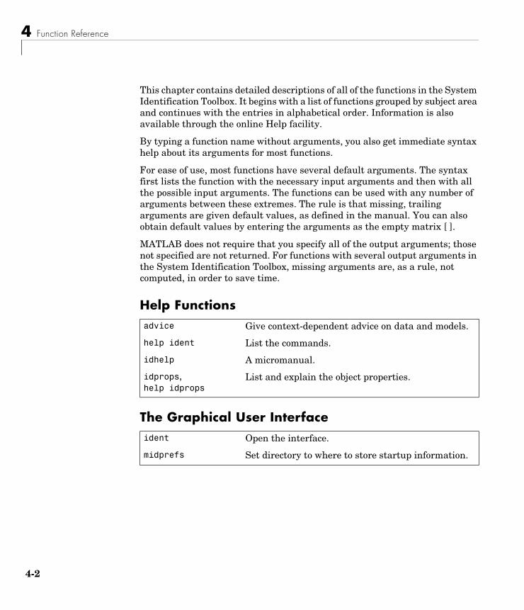
4 Function Reference
4-2
This chapter contains detailed descriptions of all of the functions in the System Identification Toolbox. It begins with a list of functions grouped by subject area and continues with the entries in alphabetical order. Information is also available through the online Help facility.
By typing a function name without arguments, you also get immediate syntax help about its arguments for most functions.
For ease of use, most functions have several default arguments. The syntax first lists the function with the necessary input arguments and then with all the possible input arguments. The functions can be used with any number of arguments between these extremes. The rule is that missing, trailing arguments are given default values, as defined in the manual. You can also obtain default values by entering the arguments as the empty matrix [ ].
MATLAB does not require that you specify all of the output arguments; those not specified are not returned. For functions with several output arguments in the System Identification Toolbox, missing arguments are, as a rule, not computed, in order to save time.
Help Functions
The Graphical User Interface
advice Give context-dependent advice on data and models.
help ident List the commands.
idhelp A micromanual.
idprops, help idprops
List and explain the object properties.
ident Open the interface.
midprefs Set directory to where to store startup information.
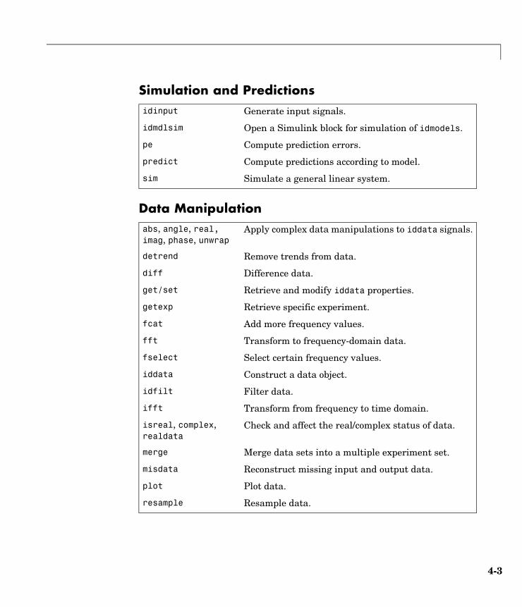
4-3
Simulation and Predictions
Data Manipulation
idinput Generate input signals.
idmdlsim Open a Simulink block for simulation of idmodels.
pe Compute prediction errors.
predict Compute predictions according to model.
sim Simulate a general linear system.
abs, angle, real, imag, phase, unwrap
Apply complex data manipulations to iddata signals.
detrend Remove trends from data.
diff Difference data.
get/set Retrieve and modify iddata properties.
getexp Retrieve specific experiment.
fcat Add more frequency values.
fft Transform to frequency-domain data.
fselect Select certain frequency values.
iddata Construct a data object.
idfilt Filter data.
ifft Transform from frequency to time domain.
isreal, complex, realdata
Check and affect the real/complex status of data.
merge Merge data sets into a multiple experiment set.
misdata Reconstruct missing input and output data.
plot Plot data.
resample Resample data.
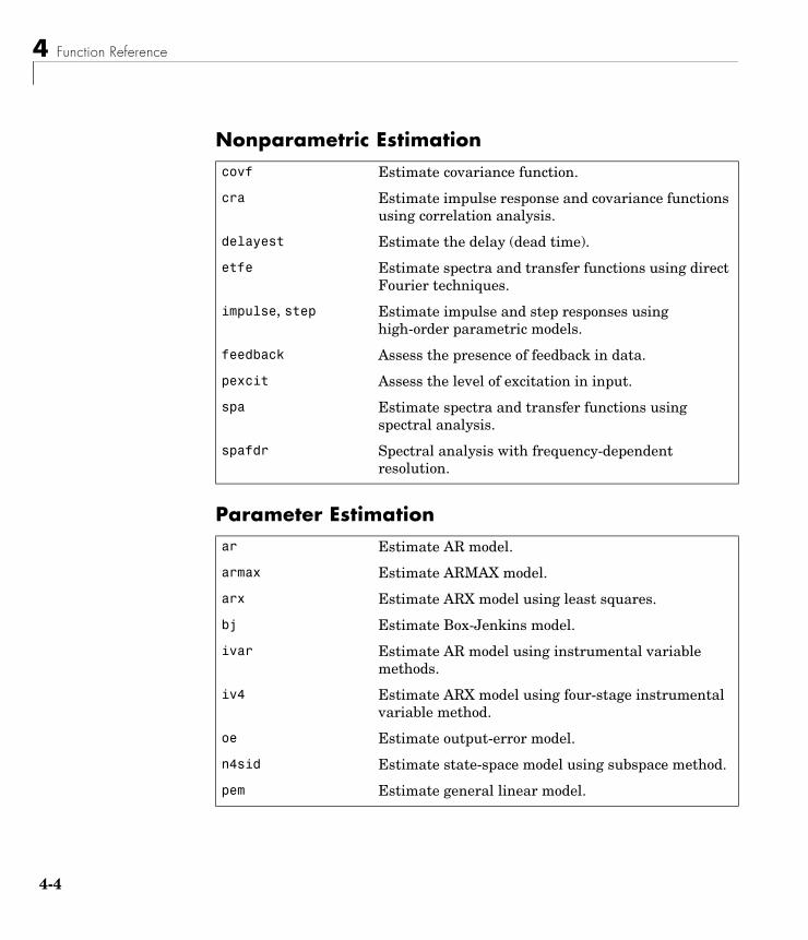
4 Function Reference
4-4
Nonparametric Estimation
Parameter Estimation
covf Estimate covariance function.
cra Estimate impulse response and covariance functions using correlation analysis.
delayest Estimate the delay (dead time).
etfe Estimate spectra and transfer functions using direct Fourier techniques.
impulse, step Estimate impulse and step responses using high-order parametric models.
feedback Assess the presence of feedback in data.
pexcit Assess the level of excitation in input.
spa Estimate spectra and transfer functions using spectral analysis.
spafdr Spectral analysis with frequency-dependent resolution.
ar Estimate AR model.
armax Estimate ARMAX model.
arx Estimate ARX model using least squares.
bj Estimate Box-Jenkins model.
ivar Estimate AR model using instrumental variable methods.
iv4 Estimate ARX model using four-stage instrumental variable method.
oe Estimate output-error model.
n4sid Estimate state-space model using subspace method.
pem Estimate general linear model.
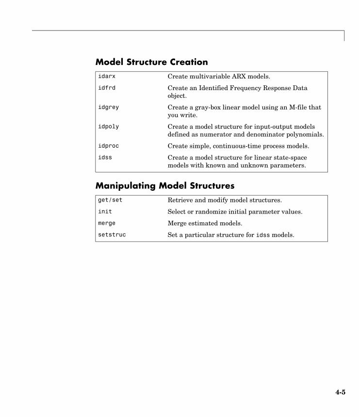
4-5
Model Structure Creation
Manipulating Model Structures
idarx Create multivariable ARX models.
idfrd Create an Identified Frequency Response Data object.
idgrey Create a gray-box linear model using an M-file that you write.
idpoly Create a model structure for input-output models defined as numerator and denominator polynomials.
idproc Create simple, continuous-time process models.
idss Create a model structure for linear state-space models with known and unknown parameters.
get/set Retrieve and modify model structures.
init Select or randomize initial parameter values.
merge Merge estimated models.
setstruc Set a particular structure for idss models.
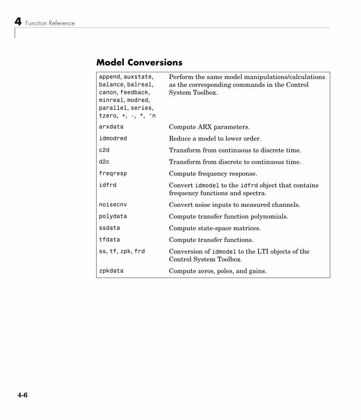
4 Function Reference
4-6
Model Conversionsappend, auxstate, balance, balreal, canon, feedback, minreal, modred, parallel, series, tzero, +, -, *, ^n
Perform the same model manipulations/calculations as the corresponding commands in the Control System Toolbox.
arxdata Compute ARX parameters.
idmodred Reduce a model to lower order.
c2d Transform from continuous to discrete time.
d2c Transform from discrete to continuous time.
freqresp Compute frequency response.
idfrd Convert idmodel to the idfrd object that contains frequency functions and spectra.
noisecnv Convert noise inputs to measured channels.
polydata Compute transfer function polynomials.
ssdata Compute state-space matrices.
tfdata Compute transfer functions.
ss, tf, zpk, frd Conversion of idmodel to the LTI objects of the Control System Toolbox.
zpkdata Compute zeros, poles, and gains.
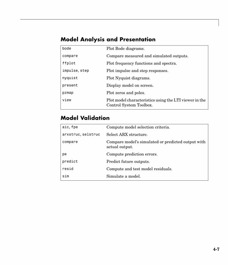
4-7
Model Analysis and Presentation
Model Validation
bode Plot Bode diagrams.
compare Compare measured and simulated outputs.
ffplot Plot frequency functions and spectra.
impulse, step Plot impulse and step responses.
nyquist Plot Nyquist diagrams.
present Display model on screen.
pzmap Plot zeros and poles.
view Plot model characteristics using the LTI viewer in the Control System Toolbox.
aic, fpe Compute model selection criteria.
arxstruc, selstruc Select ARX structure.
compare Compare model’s simulated or predicted output with actual output.
pe Compute prediction errors.
predict Predict future outputs.
resid Compute and test model residuals.
sim Simulate a model.
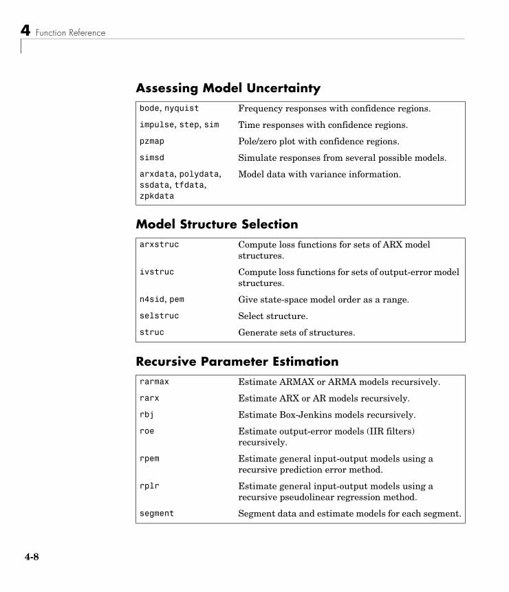
4 Function Reference
4-8
Assessing Model Uncertainty
Model Structure Selection
Recursive Parameter Estimation
bode, nyquist Frequency responses with confidence regions.
impulse, step, sim Time responses with confidence regions.
pzmap Pole/zero plot with confidence regions.
simsd Simulate responses from several possible models.
arxdata, polydata, ssdata, tfdata, zpkdata
Model data with variance information.
arxstruc Compute loss functions for sets of ARX model structures.
ivstruc Compute loss functions for sets of output-error model structures.
n4sid, pem Give state-space model order as a range.
selstruc Select structure.
struc Generate sets of structures.
rarmax Estimate ARMAX or ARMA models recursively.
rarx Estimate ARX or AR models recursively.
rbj Estimate Box-Jenkins models recursively.
roe Estimate output-error models (IIR filters) recursively.
rpem Estimate general input-output models using a recursive prediction error method.
rplr Estimate general input-output models using a recursive pseudolinear regression method.
segment Segment data and estimate models for each segment.
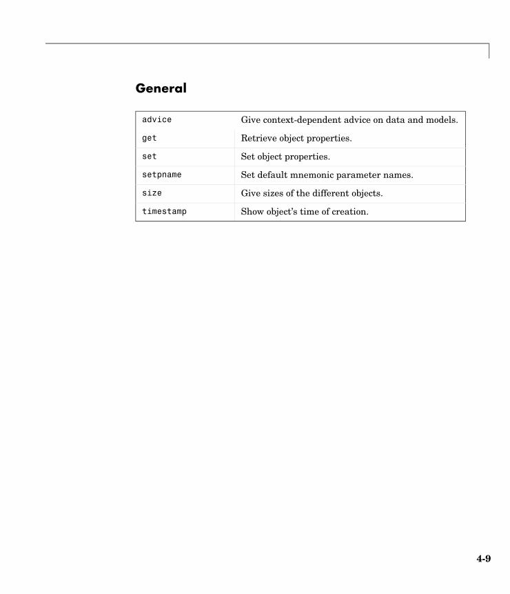
4-9
General
advice Give context-dependent advice on data and models.
get Retrieve object properties.
set Set object properties.
setpname Set default mnemonic parameter names.
size Give sizes of the different objects.
timestamp Show object’s time of creation.

4 Function Reference
4-10
advice
4-11
4 advicePurpose Give the user advice about a data set or an estimated model
Syntax advice(Model)advice(Data)
Description Model is any estimated idmodel (idarx, idgrey, idpoly, idproc, idss).
Data is any data set in the iddata format.
The command gives text information to the Command Window about the data set or the model. Typical advice given is
• For data sets,
- The excitation level of the signals and what consequences this has for what model orders can be supported (see also pexcit)
- Whether detrending should be applied
- Presence of output feedback in the data, and its consequences (see also feedback)
• For models,
- Whether the model appears to have captured the essential dynamics of the system, and/or the disturbance characteristics
- Whether the model seems to be of unnecessarily high order
- Whether significant feedback effects in the validation data can be detected
See Also feedback, pexcit
aic
4-12
4aicPurpose Compute the Akaike Information Criterion for an estimated model
Syntax am = aic(Model1,Model2,...)
Description Model is any estimated idmodel (idarx, idgrey, idpoly, idproc, idss).
am is returned as a row vector with the values of Akaike’s Information Criterion (AIC) for each of the models. The AIC is given as
where V is the loss function, d is the number of estimated parameters, and N is the number of estimation data values.
Here
(4-1)
where is the parameter estimate.
The AIC is formally defined as the value of the negative log-likelihood function at the estimated parameters plus the number of estimated parameters. The connection between this and the expressions above is as follows (cf (7.92)ff in Ljung (1999)):
If the disturbance source is Gaussian with covariance matrix , the logarithm of likelihood function is
Maximizing this analytically with regard to gives, and then maximizing the result with regard to , gives
AIC V( ) 2dN-------+log=
V det 1N---- ε t θN,( ) ε t θN,( )( )
T
1
N
∑
=
θN
Λ
L θ Λ,( ) 12---– ε t θ,( )TΛ 1– ε t θ,( ) N
2---- detlog Λ– const+
1
N
∑=
Λθ
L θ Λˆ
,( ) const Np2
-------- N2---- V( )log+ +=
aic
4-13
where p is the number of outputs and V is defined by (Equation 4-1). After removing constants and suitable normalization, the desired expression is reached.
See Also EstimationInfo, fpe
References Sections 7.4 and 16.4 in Ljung (1999).
Algorithm Properties
4-14
4Algorithm PropertiesPurpose Describe the algorithm properties that affect the estimation process
Syntax idprops algorithmm.algorithm
Description All the idmodel objects in the toolbox, idarx, idss, idpoly, idproc, and idgrey, have a property Algorithm, which is a structure that contains a number of options that govern the estimation algorithms. The fields of this structure can be individually set and retrieved in the usual way, such as get(m,'MaxIter') or m.SearchDirection = 'gn'. Also, autofill applies and the names are case insensitive.
Note Algorithm is a property of idmodel. Any algorithm property can be separately set as above. Also, if you have a standard algorithm setup that you prefer, you can set those properties simultaneously, as in m = pem(Data,mi,'alg',myalg).
Note The algorithm properties, like all other model properties, are inherited by the resulting model m. If you continue the estimation using m as the initial model, all previously set algorithm features will thus apply, unless you specify otherwise.
The fields of Algorithm are as follows:
Applying to All Estimation Methods
• Focus: This property affects the weighting applied to the fit between the model and the data. It can be used to assure that the model approximates the true system well over certain frequency intervals. Focus can assume the following values:
- 'Prediction': This is the default and means that the model is determined by minimizing the prediction errors. It corresponds to a frequency weighting that is given by the input spectrum times the inverse noise model. Typically, this favors a good fit at high frequencies. From a
Algorithm Properties
4-15
statistical variance point of view, this is the optimal weighting, but then the approximation aspects (bias) of the fit are neglected.
- 'Simulation': This means that frequency weighting of the transfer function fit is given by the input spectrum. Frequency ranges where the input has considerable power will thus be better described by the model. In other words, the model approximation is such that the model will produce as good simulations as possible, when applied to inputs with the same spectra as used for the estimation. For models that have no disturbance model, that is y = G u + e, (A=C=D=1 for idpoly models and K = 0 for idss models) there is no difference between 'Simulation' and 'Prediction'. For models with a disturbance description, that is, y = Gu + H e, G is first estimated with H = 1 and then H is estimated by a prediction error method, keeping the estimated transfer function fixed. This option also guarantees a stable transfer function G.
- 'Stability': The resulting model is guaranteed to be stable, but a prediction weighing is still maintained. Note that forcing the model to be stable could mean that a bad model is obtained. Use only when you know the system to be stable.
- A row vector or matrix defining passbands:[wl,wh] or [w1l,w1h;w2l,w2h;w3l,w3h;...]
where wl and wh define upper and lower limits for a passband. With several rows, the union of passbands defined be each row is obtained. The fit between data and model will the be focused on the passband(s) thus defined.
- Any SISO linear filter: The transfer function from input to output is determined by a frequency fit with this filter times the input spectrum as weighting function. The disturbance model is determined by a prediction error method, keeping the transfer function estimate fixed, as in the simulation case. To obtain a good model fit over a special frequency range, the filter should thus be chosen with a passband over this range. For a model with no disturbance model, the result is the same as first applying prefiltering to data using idfilt. The filter can be specified in a few different ways as
Any single-input-single-output idmodel
An ss, tf, or zpk model from the Control System Toolbox
{A,B,C,D} with the state-space matrices for the filter
G
Algorithm Properties
4-16
{numerator, denominator} with the transfer function numerator/denominator of the filter
- For frequency-domain data, 'Focus' can also be given as a column vector of weights. The vector must be of the same size as Data.Frequency. Each input and output response in the data is then multiplied by the corresponding weight at the respective frequencies.
• MaxSize: No matrix with more than MaxSize elements is formed by the algorithm, whenever possible. Instead, for loops are used. MaxSize thus decides the memory/speed tradeoff, and can prevent slow use of virtual memory. MaxSize can be any positive integer, but the input-output data must contain fewer than MaxSize elements. The default value of MaxSize is 'Auto', which means that the value is determined in the M-file idmsize. You can edit this file to optimize speed on a particular computer. Generally speaking, MaxSize does not affect the numerical properties of the estimate. The only exception is when you use InitialState = 'backcast' for frequency-domain data. Then the frequency ranges where the backcasting takes place may depend on MaxSize, resulting in slightly different estimates.
• FixedParameter: A list of parameters that will be kept fixed to the nominal/initial values and not estimated. This is a vector of integers containing the indices of the fixed parameters. The numbering of the parameters is the same as in the model property 'ParameterVector'. The parameter names from the property 'PName' can also be used. For structured state-space models, it is easier to fix/unfix parameters by the structure matrices As, Bs, etc. See idss. When you use parameter names to specify the fixed parameters, Fixedparameter is a cell array of strings. The strings can contain the wildcards '*' (meaning any continuation of the given string) and '?' (meaning any character). For example, if all disturbance model parameters start with 'k', FixedParameter = {'k*'} will fix all these parameters. The function setpname can be useful in this context.
Applying to n4sid, Estimating State-Space Models These also apply to pem for estimating black-box state-space models, since these are initialized by the n4sid estimate.
• N4Weight: This property determines some weighting matrices used in the singular-value decomposition that is a central step in the algorithm. Two choices are offered: 'MOESP', which corresponds to the MOESP algorithm by Verhaegen, and 'CVA', which is the canonical variable algorithm by
Algorithm Properties
4-17
Larimore. See the reference page for n4sid. The default value is 'N4Weight' = 'Auto', which gives an automatic choice between the two options.
• N4Horizon: Determines the prediction horizons forward and backward used by the algorithm. This is a row vector with three elements: N4Horizon = [r sy su], where r is the maximum forward prediction horizon; that is, the algorithm uses up to r step-ahead predictors. sy is the number of past outputs, and su is the number of past inputs that are used for the predictions. For an exact definition of these integers, see pages 209 and 210 in Ljung (1999), where they are called r, s1, and s2. These numbers can have a substantial influence on the quality of the resulting model, and there are no simple rules for choosing them. Making 'N4Horizon' a k-by-3 matrix means that each row of 'N4Horizon' is tried, and the value that gives the best (prediction) fit to data is selected. (This option cannot be combined with selection of model order.) If you specify only one column in 'N4Horizon', the interpretation is r=sy=su. The default choice is 'N4Horizon' = 'Auto', which uses an Akaike Information Criterion (AIC) for the selection of sy and su.
Applying to Estimation Methods Using Iterative Search for Minimizing a Criterion, That Is, armax, bj, oe, and pem
• Trace: This property determines the information about the iterative search that is provided to the MATLAB Command Window.
- 'Trace' = 'Off': No information is written to the screen.
- 'Trace' = 'On': Information about criterion values and the search process is given for each iteration.
- 'Trace' = 'Full': The current parameter values and the search direction are also given (except in the 'Free' SSParameterization case for idss models).
• LimitError: This variable determines how the criterion is modified from quadratic to one that gives linear weight to large errors. Errors larger than LimitError times the estimated standard deviation will carry a linear weight in the criterions.The default value of LimitError is 1.6. LimitError = 0 disables the robustification and leads to a purely quadratic criterion. The standard deviation is estimated robustly as the median of the absolute deviations from the median, divided by 0.7. (See Equations (15.9)

Algorithm Properties
4-18
and (15.10) in Ljung (1999).) When estimating with frequency-domain data, LimitError is set to zero.
• MaxIter: The maximum number of iterations performed during the search for minimum. The iterations stops when MaxIter is reached or some other stopping criterion is satisfied. The default value of MaxIter is 20. Setting MaxIter = 0 returns the result of the startup procedure. The actual number of used iterations is given by the property EstimationInfo.Iterations.
• Tolerance: Based on the Gauss-Newton vector computed at the current parameter value, an estimate is made of the expected improvement of the criterion at the next iteration. When this expected improvement is less than Tolerance, measured in percent, the iterations are stopped. Default value is 0.01.
• SearchDirection: The direction along which a line search is performed to find a lower value of the criterion function. It may assume the following values:
- 'gn': The Gauss-Newton direction (inverse of the Hessian times the gradient direction). If no improvement is found along this direction, the gradient direction is also tried.
- 'gns': A regularized version of the Gauss-Newton direction. Eigenvalues less than GnsPinvTol (see “Advanced” below) of the Hessian are neglected, and the Gauss-Newton direction is computed in the remaining subspace.
- 'lm': The Levenberg-Marquardt method is used. This means that the next parameter value is -pinv(H+d*I)*grad from the previous one, where H is the Hessian, I is the identity matrix, and grad is the gradient. d is a number that is increased until a lower value of the criterion is found.
- 'Auto': A choice among the above is made in the algorithm. This is the default choice.
• Advanced: This is a structure that contains detailed algorithm choices that normally the user does not need to get involved in. For detailed explanations, you must examine the code. 'Advanced' has the following fields:
- Search: Contains fields with relevance for the iterative search:a GnsPinvTol: The tolerance for the pseudoinverse used to compute the gns
direction. See above. Default is 10^-9.
b LmStep: The next value of d in the LM method is lmstep times the previous one. Default is LmStep = 2.
Algorithm Properties
4-19
c StepReduction: In the line search used for directions other than LM, the step is reduced by the factor StepReduction in each try. Default is StepReduction = 2.
d MaxBisection: The maximum number of bisections used by the line search along the search direction. Default is 10.
e LmStartValue: The starting value of d in the LM method. Default is 0.001.
f RelImprovement: The iterations are stopped if the relative improvement of the criterion is less than RelImprovement. Default is RelImprovement = 0.
- Threshold: Contains fields with thresholds for several tests:a Sstability: used for stability test of continuous-time models. Model is
considered stable if its rightmost pole is to the left of Sstability. Default is 0.
b Zstability: used for stability test of discrete-time models. Model is considered stable if all poles are within the distance Zstability from the origin. Default is 1.01.
- AutoInitialState: When InitialState = 'Auto', the state is estimated if the ratio of the prediction error norm with zero initial state to the norm with estimated initial state exceeds AutoInitialState. Default is 1.2.
See Also armax, bj, EstimationInfo, n4sid, oe, pem
References For the iterative minimization, see Dennis, J.E., Jr., and R.B. Schnabel, Numerical Methods for Unconstrained Optimization and Nonlinear Equations, Prentice Hall, Englewood Cliffs, N.J., 1983.
For a general reference to the identification algorithms, see Ljung (1999), Chapter 10.

ar
4-20
4arPurpose Estimate the parameters of an AR model for scalar time series
Syntax m = ar(y,n)[m ,refl] = ar(y,n,approach,window)[m,refl] = ar(y,n,approach,window,Prop1,Value1,Prop2,Value2,...)
Description The parameters of the AR model structure
are estimated using variants of the least squares method.
The iddata object y contains the time-series data (just one output channel). The scalar n specifies the order of the model to be estimated (the number of A parameters in the AR model).
Note that the routine is for scalar time series only. For multivariate data use arx.
The estimate is returned in m and stored as an idpoly model. For the two lattice-based approaches, 'burg' and 'gl' (see below), the variable refl is returned, containing the reflection coefficients in the first row and the corresponding loss function values in the second. The first column is the zeroth-order model, so that the (2,1) element of refl is the norm of the time series itself.
Variable approach allows you to choose an algorithm from a group of several popular techniques for computing the least squares AR model. Available methods are as follows:
approach = 'fb': The forward-backward approach. This is the default approach. The sum of a least squares criterion for a forward model and the analogous criterion for a time-reversed model is minimized.
approach = 'ls': The least squares approach. The standard sum of squared forward prediction errors is minimized.
approach = 'yw': The Yule-Walker approach. The Yule-Walker equations, formed from sample covariances, are solved.
approach = 'burg': Burg’s lattice-based method. The lattice filter equations are solved using the harmonic mean of forward and backward squared prediction errors.
A q( )y t( ) e t( )=
ar
4-21
approach = 'gl': A geometric lattice approach. As in Burg’s method, but the geometric mean is used instead of the harmonic one.
Windowing, within the context of AR modeling, is a technique for dealing with the fact that information about past and future data is lacking. There are a number of variants available:
window = 'now': No windowing. This is the default value, except when approach = 'yw'. Only actually measured data are used to form the regression vectors. The summation in the criteria starts only at time n.
window = 'prw': Prewindowing. Missing past data are replaced by zeros, so that the summation in the criteria can be started at time zero.
window = 'pow': Postwindowing. Missing end data are replaced by zeros, so that the summation can be extended to time N + n (N being the number of observations).
window = 'ppw': Pre- and postwindowing. This is used in the Yule-Walker approach.
The combinations of approaches and windowing have a variety of names. The least squares approach with no windowing is also known as the covariance method. This is the same method that is used in the arx routine. The MATLAB default method, forward-backward with no windowing, is often called the modified covariance method. The Yule-Walker approach, least squares plus pre- and postwindowing, is also known as the correlation method.
Possible property name/property value pairs are
- 'MaxSize'/Integer. See Algorithm Properties for an explanation of maxsize.
- 'Ts'/Real positive number. Setting the sampling time (overriding the sampling time of y.
- 'Covariance'/'None': Suppressing the calculation of the covariance matrix.
Examples Compare the spectral estimates of Burg’s method with those found from the forward-backward nonwindowed method, given a sinusoid in noise signal.
y = sin([1:300]') + 0.5*randn(300,1);y = iddata(y);

ar
4-22
mb = ar(y,4,'burg');mfb = ar(y,4);bode(mb,mfb)
See Also arx, etfe, ivar, spa
References Marple, Jr., S. L., Digital Spectral Analysis with Applications, Prentice Hall, Englewood Cliffs, 1987, Chapter 8.
armax
4-23
4armaxPurpose Estimate the parameters of an ARMAX or ARMA model
Syntax m = armax(data,orders)m = armax(data,'na',na,'nb',nb,'nc',nc,'nk',nk)m = armax(data,orders,'Property1',Value1,...,'PropertyN',ValueN)
Description armax returns m as an idpoly object with the resulting parameter estimates, together with estimated covariances.
armax estimates the parameters of the ARMAX model structure
using a prediction error method.
data is an iddata object containing the output-input data. Only time domain data are supported by armax. Use oe for frequency-domain data instead.The model orders can be specified as (...,'na',na,'nb',nb,...) or by setting the argument orders to
orders = [na nb nc nk]
The parameters na, nb, and nc are the orders of the ARMAX model, and nk is the delay. Specifically,
Alternatively, you can specify the vector as
orders = mi
where mi is an initial guess at the ARMAX model given in idpoly format. See “Polynomial Representation of Transfer Functions” on page 3-11 for more information.
For multiinput systems, nb and nk are row vectors, such that the kth entry corresponds to the order and delay associated with the kth input.
A q( )y t( ) B q( )u t nk–( ) C q( )e t( )+=
na: A q( ) 1 a1q 1– … anaq na–+ + +=
nb: B q( ) b1 b+ 2q 1– … bnbq nb– 1++ +=
nc: C q( ) 1 c1q 1– … cncq nc–+ + +=
armax
4-24
If data has no input channels and just one output channel (that is, it is a time series), then
orders = [na nc]
and armax calculates an ARMA model for the time series
The structure and the estimation algorithm are affected by any property name/property value pairs that are set in the input argument list. Useful properties are 'Focus', 'InitialState', 'Trace', 'MaxIter', 'Tolerance', 'LimitError', and 'FixedParameter'.
See Algorithm Properties, idpoly, and idmodel for details of these properties and their possible values.
armax does not support multioutput models. Use the state-space model for this case (see n4sid and pem).
Algorithm A robustified quadratic prediction error criterion is minimized using an iterative search algorithm, whose details are governed by the properties 'SearchDirection', 'MaxIter', 'Tolerance', and 'Advanced'. The iterations are terminated when MaxIter is reached, when the expected improvement is less than Tolerance, or when a lower value of the criterion cannot be found. Information about the search is contained in m.EstimationInfo.
The initial parameter values for the iterative search, if not specified in orders, are constructed in a special four-stage LS-IV algorithm.
The cutoff value for the robustification is based on the property LimitError as well as on the estimated standard deviation of the residuals from the initial parameter estimate. It is not recalculated during the minimization.
A stability test of the predictor is performed to ensure that only models corresponding to stable predictors are tested. Generally, both and (if applicable) must have all their zeros inside the unit circle.
Information about the minimization is furnished to the screen in case the property 'Trace' is set to 'On' or 'Full'. With 'Trace' = 'Full', current and previous parameter estimates (in column vector form, listing parameters in alphabetical order) as well as the values of the criterion function are given. The
A q( )y t( ) C q( )e t( )=
C q( ) Fi q( )
armax
4-25
Gauss-Newton vector and its norm are also displayed. With 'Trace' = 'On' just criterion values are displayed.
See Also arx, bj, idmodel, idpoly, oe, pem, Algorithm Properties, EstimationInfo
References Ljung (1999), Section 10.2.
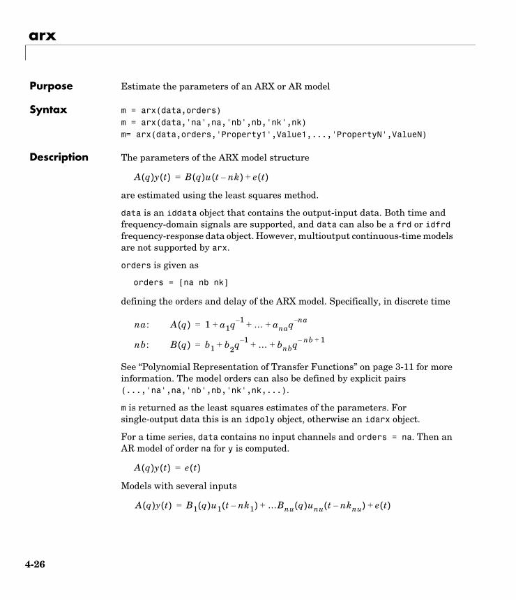
arx
4-26
4arxPurpose Estimate the parameters of an ARX or AR model
Syntax m = arx(data,orders)m = arx(data,'na',na,'nb',nb,'nk',nk)m= arx(data,orders,'Property1',Value1,...,'PropertyN',ValueN)
Description The parameters of the ARX model structure
are estimated using the least squares method.
data is an iddata object that contains the output-input data. Both time and frequency-domain signals are supported, and data can also be a frd or idfrd frequency-response data object. However, multioutput continuous-time models are not supported by arx.
orders is given as
orders = [na nb nk]
defining the orders and delay of the ARX model. Specifically, in discrete time
See “Polynomial Representation of Transfer Functions” on page 3-11 for more information. The model orders can also be defined by explicit pairs (...,'na',na,'nb',nb,'nk',nk,...).
m is returned as the least squares estimates of the parameters. For single-output data this is an idpoly object, otherwise an idarx object.
For a time series, data contains no input channels and orders = na. Then an AR model of order na for y is computed.
Models with several inputs
A q( )y t( ) B q( )u t nk–( ) e t( )+=
na: A q( ) 1 a+ 1q 1– … anaq na–+ +=
nb: B q( ) b1 b+ 2q 1– … bnbq nb– 1++ +=
A q( )y t( ) e t( )=
A q( )y t( ) B1 q( )u1 t nk1–( ) …Bnu q( )unu t nknu–( ) e t( )+ +=
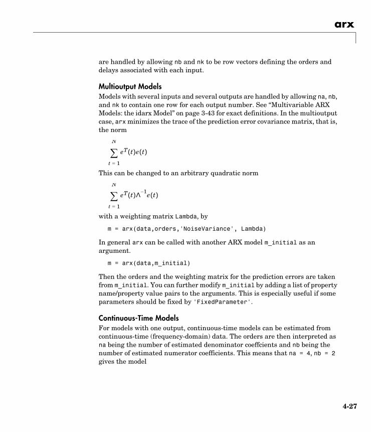
arx
4-27
are handled by allowing nb and nk to be row vectors defining the orders and delays associated with each input.
Multioutput ModelsModels with several inputs and several outputs are handled by allowing na, nb, and nk to contain one row for each output number. See “Multivariable ARX Models: the idarx Model” on page 3-43 for exact definitions. In the multioutput case, arx minimizes the trace of the prediction error covariance matrix, that is, the norm
This can be changed to an arbitrary quadratic norm
with a weighting matrix Lambda, by
m = arx(data,orders,'NoiseVariance', Lambda)
In general arx can be called with another ARX model m_initial as an argument.
m = arx(data,m_initial)
Then the orders and the weighting matrix for the prediction errors are taken from m_initial. You can further modify m_initial by adding a list of property name/property value pairs to the arguments. This is especially useful if some parameters should be fixed by 'FixedParameter'.
Continuous-Time ModelsFor models with one output, continuous-time models can be estimated from continuous-time (frequency-domain) data. The orders are then interpreted as na being the number of estimated denominator coeffcients and nb being the number of estimated numerator coefficients. This means that na = 4, nb = 2 gives the model
eT t( )e t( )
t 1=
N
∑
eT t( )Λ 1– e t( )
t 1=
N
∑
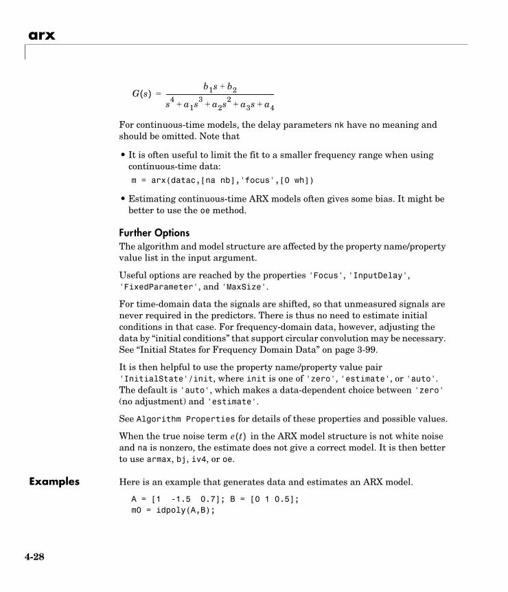
arx
4-28
For continuous-time models, the delay parameters nk have no meaning and should be omitted. Note that
• It is often useful to limit the fit to a smaller frequency range when using continuous-time data:m = arx(datac,[na nb],'focus',[0 wh])
• Estimating continuous-time ARX models often gives some bias. It might be better to use the oe method.
Further OptionsThe algorithm and model structure are affected by the property name/property value list in the input argument.
Useful options are reached by the properties 'Focus', 'InputDelay', 'FixedParameter', and 'MaxSize'.
For time-domain data the signals are shifted, so that unmeasured signals are never required in the predictors. There is thus no need to estimate initial conditions in that case. For frequency-domain data, however, adjusting the data by “initial conditions” that support circular convolution may be necessary. See “Initial States for Frequency Domain Data” on page 3-99.
It is then helpful to use the property name/property value pair 'InitialState'/init, where init is one of 'zero', 'estimate', or 'auto'. The default is 'auto', which makes a data-dependent choice between 'zero' (no adjustment) and 'estimate'.
See Algorithm Properties for details of these properties and possible values.
When the true noise term in the ARX model structure is not white noise and na is nonzero, the estimate does not give a correct model. It is then better to use armax, bj, iv4, or oe.
Examples Here is an example that generates data and estimates an ARX model.
A = [1 -1.5 0.7]; B = [0 1 0.5];m0 = idpoly(A,B);
G s( )b1s b2+
s4 a1s3 a2s2 a3s a4+ + + +-----------------------------------------------------------------------=
e t( )

arx
4-29
u = iddata([],idinput(300,'rbs'));e = iddata([],randn(300,1));y = sim(m0, [u e]);z = [y,u];m = arx(z,[2 2 1]);
Algorithm The least squares estimation problem is an overdetermined set of linear equations that is solved using QR factorization.
The regression matrix is formed so that only measured quantities are used (no fill-out with zeros). When the regression matrix is larger than MaxSize, the QR factorization is performed in a for loop.
See Also ar, ivx, iv4, Algorithm Properties, EstimationInfo
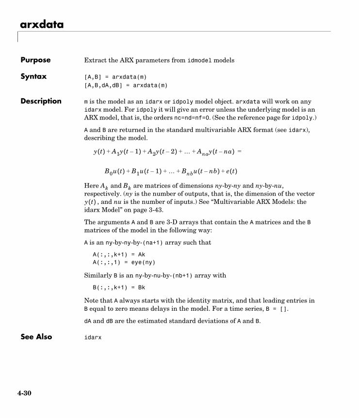
arxdata
4-30
4arxdataPurpose Extract the ARX parameters from idmodel models
Syntax [A,B] = arxdata(m)[A,B,dA,dB] = arxdata(m)
Description m is the model as an idarx or idpoly model object. arxdata will work on any idarx model. For idpoly it will give an error unless the underlying model is an ARX model, that is, the orders nc=nd=nf=0. (See the reference page for idpoly.)
A and B are returned in the standard multivariable ARX format (see idarx), describing the model.
Here and are matrices of dimensions ny-by-ny and ny-by-nu, respectively. (ny is the number of outputs, that is, the dimension of the vector
, and nu is the number of inputs.) See “Multivariable ARX Models: the idarx Model” on page 3-43.
The arguments A and B are 3-D arrays that contain the A matrices and the B matrices of the model in the following way:
A is an ny-by-ny-by-(na+1) array such that
A(:,:,k+1) = AkA(:,:,1) = eye(ny)
Similarly B is an ny-by-nu-by-(nb+1) array with
B(:,:,k+1) = Bk
Note that A always starts with the identity matrix, and that leading entries in B equal to zero means delays in the model. For a time series, B = [].
dA and dB are the estimated standard deviations of A and B.
See Also idarx
y t( ) A1y t 1–( ) A2y t 2–( ) … Anay t na–( )+ + + + =
B0u t( ) B1u t 1–( ) … Bnbu t nb–( ) e t( )+ + + +
Ak Bk
y t( )
arxstruc
4-31
4arxstrucPurpose Compute loss functions for a set of different model structures of single-output ARX type
Syntax V = arxstruc(ze,zv,NN)V = arxstruc(ze,zv,NN,maxsize)
Description NN is a matrix that defines a number of different structures of the ARX type. Each row of NN is of the form
nn = [na nb nk]
with the same interpretation as described for arx. See struc for easy generation of typical NN matrices for single-input systems.
Each of ze and zv is an iddata object containing output-input data. Frequency-domain data and idfrd objects are also supported. Models for each of the model structures defined by NN are estimated using the data set ze. The loss functions (normalized sum of squared prediction errors) are then computed for these models when applied to the validation data set zv. The data sets ze and zv need not be of equal size. They could, however, be the same sets, in which case the computation is faster.
Note that arxstruc is intended for single-output systems only.
The output argument V is best analyzed using selstruc. It contains the loss functions in its first row. The remaining rows of V contain the transpose of NN, so that the orders and delays are given just below the corresponding loss functions. The last column of V contains the number of data points in ze. The selection of a suitable model structure based on the information in v is normally done using selstruc. See “Model Structure Selection and Validation” on page 3-70 for advice on model structure selection and cross validation.
See Algorithm Properties for an explanation of maxsize.
Examples Compare first- to fifth-order models with one delay using cross validation on the second half of the data set. Then select the order that gives the best fit to the validation data set.
NN = struc(1:5,1:5,1);V = arxstruc(z(1:200),z(201:400),NN);nn = selstruc(V,0);m = arx(z,nn);

arxstruc
4-32
See Also arx, ivstruc, n4sid, selstruc, struc
bj
4-33
4bjPurpose Estimate the parameters of a Box-Jenkins model
Syntax m = bj(data,orders)m = bj(data,'nb',nb,'nc',nc,'nd',nd,'nf',nf,'nk',nk)m = bj(data,orders,'Property1',Value1,'Property2',Value2,...)
Description bj returns m as an idpoly object with the resulting parameter estimates, together with estimated covariances. The bj function estimates parameters of the Box-Jenkins model structure
using a prediction error method.
data is an iddata object containing the output-input data. Frequency-domain signals are not supported by bj. Use oe instead.
The model orders can be specified by setting the argument orders to
orders = [ nb nc nd nf nk]
The parameters nb, nc, nd, and nf are the orders of the Box-Jenkins model and nk is the delay. Specifically,
The orders can also be defined as property name/property value pairs (...,'nb',nb,...). Alternatively, you can specify the vector as
orders = mi
where mi is an initial guess at the Box-Jenkins model given in idpoly format. See “Polynomial Representation of Transfer Functions” on page 3-11 for more information.
y t( ) B q( )F q( )------------u t nk–( ) C q( )
D q( )-------------e t( )+=
nf: F q( ) 1 f+ 1q 1– … fnfqnf–+ +=
nb: B q( ) b1 b+ 2q 1– … bnbq nb– 1++ +=
nc: C q( ) 1 c+ 1q 1– … cncq nc–+ +=
nd: D q( ) 1 d+ 1q 1– … dndq nd–+ +=
bj
4-34
For multiinput systems, nb, nf, and nk are row vectors with as many entries as there are input channels. Entry number i then describes the orders and delays associated with the ith input.
The structure and the estimation algorithm are affected by any property name/property value pairs that are set in the input argument list. Useful properties are 'Focus', 'InitialState', 'Trace', 'MaxIter', 'Tolerance', 'LimitError', and 'FixedParameter'.
See Algorithm Properties and the reference pages for idmodel and idpoly for details of these properties and their possible values.
bj does not support multioutput models. Use a state-space model for this case (see n4sid and pem).
Examples Here is an example that generates data and stores the results of the startup procedure separately.
B = [0 1 0.5];C = [1 -1 0.2];D = [1 1.5 0.7];F = [1 -1.5 0.7];m0 = idpoly(1,B,C,D,F,0.1);e = iddata([],randn(200,1));u = iddata([],idinput(200)); y = sim(m0,[u e]);z = [y u];mi = bj(z,[2 2 2 2 1],'MaxIter',0)m = bj(z,mi,'Maxi',10)m.EstimationInfom = bj(z,m); % Continue if m.es.WhyStop shows that maxiter has
% been reached.compare(z,m,mi)
Algorithm bj uses essentially the same algorithm as armax with modifications to the computation of prediction errors and gradients.
See Also armax, idmodel, idpoly, oe, pem
bode
4-35
4bodePurpose Plot frequency functions in Bode diagram form
Syntax bode(m)[mag,phase,w] = bode(m)[mag,phase,w,sdmag,sdphase] = bode(m)bode(m1,m2,m3,...,w)bode(m1,'PlotStyle1',m2,'PlotStyle2',...)bode(m1,m2,m3,..'sd',sd,'mode',mode,'ap',ap)bode(m1,m2,m3,'sd',sd,'mode',mode,'ap',ap,'fill')
Description bode computes the magnitude and phase of the frequency response of idmodel and idfrd models. When invoked without left-hand arguments, bode produces a Bode plot on the screen.
bode(m) plots the Bode response of an arbitrary idmodel or idfrd model m. This model can be continuous or discrete, and SISO or MIMO. The InputNames and OuputNames properties of the models are used to plot the responses for different I/O channels in separate plots. Pressing the Enter key advances the plot from one input-output pair to the next one. Typing Ctrl+C aborts the plotting in an orderly fashion
If m contains information about both I/O channels and output noise spectra, only the I/O channels are shown. To show the output noise spectra, enter m('n') ('n' for 'noise') in the model list. Analogously, you can select specific I/O channels with normal subreferencing m(ky,ku).
Argument wbode(m,w) explicitly specifies the frequency range or frequency points to be used for the plot or for computing the response.
To focus on a particular frequency interval [wmin,wmax], set w = {wmin,wmax} (notice the curly brackets). This plots the response for 100 frequency points logarithmically spaced from wmin to wmax. You can change this to NP points by using w = {wmin,wmax,NP}.
To use particular frequency points, set w to the vector of desired frequencies. Use logspace to generate logarithmically spaced frequency vectors. All frequencies should be specified in rad/s.
bode
4-36
Note that the frequencies cannot be specified for idfrd objects. For those the plot and response are calculated for the internally stored frequencies. However, the plot is restricted to the range {wmin,wmax} if this is specified.
If no frequency range is specified, a default choice is made based on the dynamics of the model.
Property Name/Property Value Pairs 'sd'/sd, 'ap'/ap, and 'mode'/modeThe pairs can appear in any order or be omitted.
• sd: If sd is specified as a number larger than zero, confidence intervals for the functions are added to the graph as dash-dotted curves (of the same color as the estimate curve). They indicate the confidence regions corresponding to sd standard deviations. If an argument 'fill' is included in the argument list, the confidence region is marked as a filled band instead.
• ap: By default, amplitude and phase plots are shown simultaneously for each I/O channel present in m. For spectra, phase plots are omitted. To show amplitude plots only, use ap = 'A'. For phase plots only, use ap = 'P'. The default is ap = 'B' for both plots.
• mode: To obtain all input/output plots in the same diagram use mode = 'same'.
Several Modelsbode(m1,m2,...,mN) or bode(m1,m2,...mN,w) plots the Bode response of several idmodel or idfrd models on a single figure. The models can be mixes of different sizes and continuous/discrete. The sorting of the plots is based on the InputNames and OutputNames. If the frequencies w are specified, these will apply to all non-idfrd models in the list. If you want different frequencies for different models, you should thus first convert them to idfrd objects using the idfrd command.
bode(m1,'PlotStyle1',...,mN,'PlotStyleN') further specifies which color, line style, and/or marker should be used to plot each system, as in
bode(m1,'r--',m2,'gx')
Arguments The output argument w contains the frequencies for which the response is given, whether specified among the input arguments or not. The output arguments mag and phase are 3-D arrays with dimensions
bode
4-37
(number of outputs)x(number of inputs)x(length of w)
For SISO systems, mag(1,1,k) and phase(1,1,k) give the magnitude and phase (in degrees) at the frequency = w(k). To obtain the result as a normal vector of responses, use mag = mag(:) and phase = phase(:).
For MIMO systems, mag(i,j,k) is the magnitude of the frequency response at frequency w(k) from input j to output i, and similarly for phase(i,j,k).
If sdmag and sdphase are specified, the standard deviations of the magnitude and phase are also computed. Then sdmag is an array of the same size as mag, containing the estimated standard deviations of the response, and analogously for sdphase.
See Also etfe, freqresp, idfrd, nyquist, spa, spafdr
ωk

compare
4-38
4comparePurpose Compare measured outputs with model outputs
Syntax compare(data,m);compare(data,m,k)compare(data,m,k,'Samples',sampnr,'InitialState',init,'OutputPlots
',Yplots)compare(data,m1,m2,...,mN)compare(data,m1,'PlotStyle1',...,mN,'PlotStyleN')[yh,fit] = compare(data,m1,'PlotStyle1',...,mN,'PlotStyleN',k)
Description data is the output-input data in the usual iddata object format. data can also be an idfrd object with frequency-response data.
compare computes the output yh that results when the model m is simulated with the input u. The result is plotted together with the corresponding measured output y. The percentage of the output variation that is explained by the model
fit = 100*(1 - norm(yh - y)/norm(y-mean(y)))
is also computed and displayed. For multioutput systems, this is done separately for each output. For frequency-domain data (or in general for complex valued data) the fit is still calculated as above, but only the absolute values of y and yh are plotted.
When the argument k is specified, the k step-ahead prediction of y according to the model m are computed instead of the simulated output. In the calculation of
, the model can use outputs up to time : , , (and inputs up to the current time t). The default value of k is inf, which gives a pure simulation from the input only. Note that for frequency-domain data only simulation (k = inf) is allowed, and for time-series data (no input) only prediction (k not inf) is possible.
Property Name/Property Value PairsThe optional property name/property value pairs 'Samples'/sampnr, 'InitialState'/init, and 'OutputPlots'/Yplots can be given in any order.
The argument Yplots can be a cell array of strings. Only the outputs with OutputName in this array are plotted, while all are used for the necessary computations. If Yplots is not specified, all outputs are plotted.
yh t( ) t k– y s( ) s, t k–= t k– 1– …
compare
4-39
The argument sampnr indicates that only the sample numbers in this row vector are plotted and used for the calculation of the fit. The whole data record is used for the simulation/prediction.
The argument init determines how to handle initial conditions in the models:
• init = 'e' (for 'estimate') estimates the initial conditions for best fit.
• init = 'm' (for 'model') used the model’s internally stored initial state.
• init = 'z' (for 'zero') uses zero initial conditions.
• init = x0, where x0 is a column vector of the same size as the state vector of the models, uses x0 as the initial state.
• init = 'e' is the default.
Several ModelsWhen several models are specified, as in compare(data,m1,m2,...,mN), the plots show responses and fits for all models. In that case data should contain all inputs and outputs that are required for the different models. However, some models might correspond to subselections of channels and might not need all channels in data. In that case the proper handling of signals is based on the InputNames and OutputNames of data and the models.
With compare(data,m1,'PlotStyle1',...mN,'PlotStyle2'), the color, line style, and/or marker can be specified for the curves associated with the different models. The markers are the same as for the regular plot command. For example,
compare(data,m1,'g_*',m2,'r:')
If data contains several experiments, separate plots are given for the different experiments. In this case sampnr, if specified, must be a cell array with as many entries as there are experiments.
Arguments When output arguments [yh,fit] = compare(data,m1,..,mN) are specified, no plots are produced.
yh is a cell array of length equal to the number of models. Each cell contains the corresponding model output as an iddata object.
fit is, in the general case, a 3-D array with fit(kexp,kmod,ky) containing the fit (computed as above) for output ky, model kmod, and experiment kexp.
compare
4-40
Examples Split the data record into two parts. Use the first one for estimating a model and the second one to check the model’s ability to predict six steps ahead.
ze = z(1:250);zv = z(251:500);m= armax(ze,[2 3 1 0]);compare(zv,m,6);compare(zv,m,6,'Init','z') % No estimation of the initial state.
See Also sim, predict
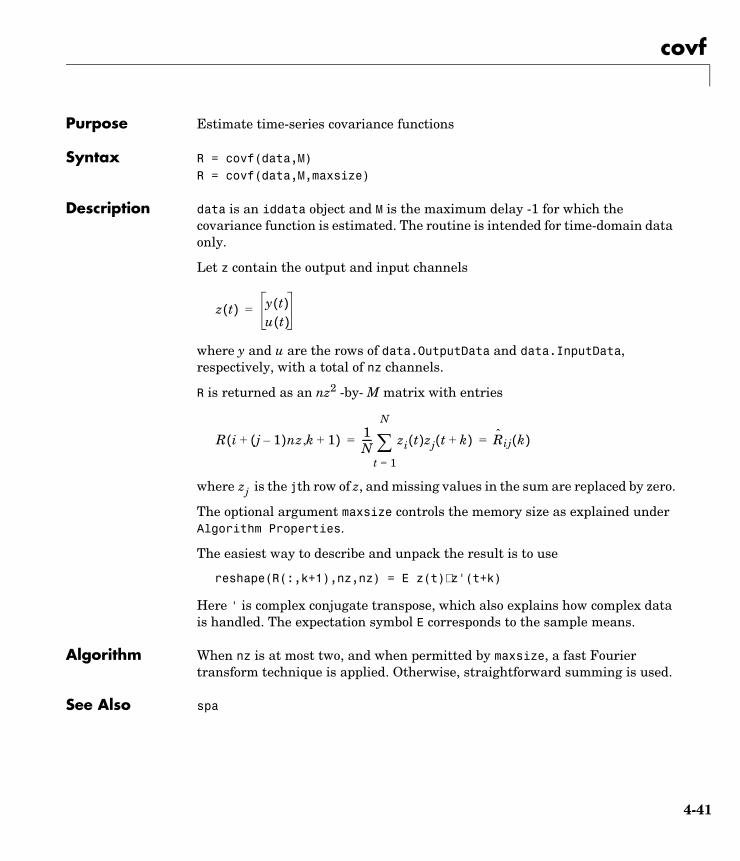
covf
4-41
4covfPurpose Estimate time-series covariance functions
Syntax R = covf(data,M)R = covf(data,M,maxsize)
Description data is an iddata object and M is the maximum delay -1 for which the covariance function is estimated. The routine is intended for time-domain data only.
Let z contain the output and input channels
where y and u are the rows of data.OutputData and data.InputData, respectively, with a total of nz channels.
R is returned as an nz2 -by- M matrix with entries
where is the jth row of z, and missing values in the sum are replaced by zero.
The optional argument maxsize controls the memory size as explained under Algorithm Properties.
The easiest way to describe and unpack the result is to use
reshape(R(:,k+1),nz,nz) = E z(t)∗ z'(t+k)
Here ' is complex conjugate transpose, which also explains how complex data is handled. The expectation symbol E corresponds to the sample means.
Algorithm When nz is at most two, and when permitted by maxsize, a fast Fourier transform technique is applied. Otherwise, straightforward summing is used.
See Also spa
z t( ) y t( )u t( )
=
R i j 1–( )nz k 1+,+( ) 1N---- zi t( )zj t k+( )
t 1=
N
∑ Rij k( )= =
zj
cra
4-42
4craPurpose Perform prewhitening-based correlation analysis and estimate impulse response
Syntax cra(data);[ir,R,cl] = cra(data,M,na,plot);cra(R);
Description data is the output-input data given as an iddata object. The routine is intended for time-domain data only.
The routine only handles single-input-single-output data pairs. (For the multivariate case, apply cra to two signals at a time, or use impulse.) cra prewhitens the input sequence; that is, cra filters u through a filter chosen so that the result is as uncorrelated (white) as possible. The output y is subjected to the same filter, and then the covariance functions of the filtered y and u are computed and graphed. The cross correlation function between (prewhitened) input and output is also computed and graphed. Positive values of the lag variable then correspond to an influence from u to later values of y. In other words, significant correlation for negative lags is an indication of feedback from y to u in the data.
A properly scaled version of this correlation function is also an estimate of the system’s impulse response ir. This is also graphed along with 99% confidence levels. The output argument ir is this impulse response estimate, so that its first entry corresponds to lag zero. (Negative lags are excluded in ir.) In the plot, the impulse response is scaled so that it corresponds to an impulse of height 1/T and duration T, where T is the sampling interval of the data.
The output argument R contains the covariance/correlation information as follows:
• The first column of R contains the lag indices.
• The second column contains the covariance function of the (possibly filtered) output.
• The third column contains the covariance function of the (possibly prewhitened) input.
• The fourth column contains the correlation function. The plots can be redisplayed by cra(R).
cra
4-43
The output argument cl is the 99% confidence level for the impulse response estimate.
The optional argument M defines the number of lags for which the covariance/correlation functions are computed. These are from -M to M, so that the length of R is 2M+1. The impulse response is computed from 0 to M. The default value of M is 20.
For the prewhitening, the input is fitted to an AR model of order na. The third argument of cra can change this order from its default value na = 10. With na = 0 the covariance and correlation functions of the original data sequences are obtained.
plot: plot = 0 gives no plots. plot = 1 (the default) gives a plot of the estimated impulse response together with a 99% confidence region. plot = 2 gives a plot of all the covariance functions.
An often better alternative to cra is the functions impulse and step, which use a high-order FIR model to estimate the impulse response.
Examples Compare a second-order ARX model’s impulse response with the one obtained by correlation analysis.
ir = cra(z);m = arx(z,[2 2 1]);imp = [1;zeros(19,1)];irth = sim(m,imp);subplot(211)plot([ir irth])title('impulse responses')subplot(212)plot([cumsum(ir),cumsum(irth)])title('step responses')
See Also impulse, step
c2d
4-44
4c2dPurpose Convert a model from continuous time to discrete time
Syntax md = c2d(mc,T)md = c2d(mc,T,method)
Description mc is a continuous-time model such as any idmodel object (idgrey, idproc, idpoly, or idss). md is the model that is obtained when it is sampled with sampling interval T.
method = 'zoh' (default) makes the translation to discrete time under the assumption that the input is piecewise constant (zero-order hold).
method = 'foh' assumes the input to be piecewise linear between the sampling instants (first-order hold).
With the Control System Toolbox, methods 'tustin', 'prewarp', and 'matched' are also supported. In these cases the covariance matrix is not transformed.
Note that the innovations variance of the continuous-time model is interpreted as the intensity of the spectral density of the noise spectrum. The noise variance in md is thus given as /T.
idpoly and idss models are returned in the same format. idgrey structures are preserved if their CDMfile property is equal to 'cd'. Otherwise they are transformed to idss objects.
Examples Define a continuous-time system and study the poles and zeros of the sampled counterpart.
mc = idpoly(1,1,1,1,[1 1 0],'Ts',0);md = c2d(mc,0.5);pzmap(md)
See Also Purpose
λ
λ
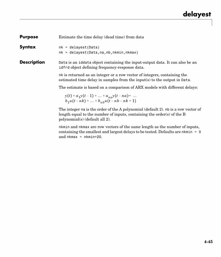
delayest
4-45
4delayestPurpose Estimate the time delay (dead time) from data
Syntax nk = delayest(Data)nk = delayest(Data,na,nb,nkmin,nkmax)
Description Data is an iddata object containing the input-output data. It can also be an idfrd object defining frequency-response data.
nk is returned as an integer or a row vector of integers, containing the estimated time delay in samples from the input(s) to the output in Data.
The estimate is based on a comparison of ARX models with different delays:
The integer na is the order of the A polynomial (default 2). nb is a row vector of length equal to the number of inputs, containing the order(s) of the B polynomial(s) (default all 2).
nkmin and nkmax are row vectors of the same length as the number of inputs, containing the smallest and largest delays to be tested. Defaults are nkmin = 0 and nkmax = nkmin+20.
y t( ) a1y t 1–( ) … anay t na–( ) …b1u t nk–( ) … bnbu t nb– nk– 1+( )+ +
=+ + +
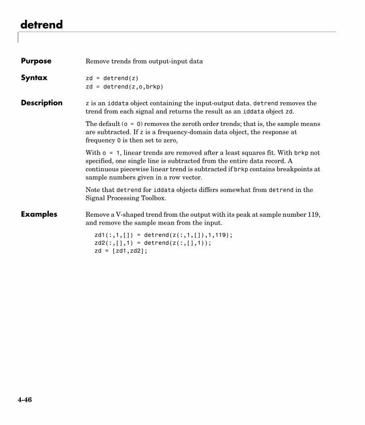
detrend
4-46
4detrend Purpose Remove trends from output-input data
Syntax zd = detrend(z)zd = detrend(z,o,brkp)
Description z is an iddata object containing the input-output data. detrend removes the trend from each signal and returns the result as an iddata object zd.
The default (o = 0) removes the zeroth order trends; that is, the sample means are subtracted. If z is a frequency-domain data object, the response at frequency 0 is then set to zero,
With o = 1, linear trends are removed after a least squares fit. With brkp not specified, one single line is subtracted from the entire data record. A continuous piecewise linear trend is subtracted if brkp contains breakpoints at sample numbers given in a row vector.
Note that detrend for iddata objects differs somewhat from detrend in the Signal Processing Toolbox.
Examples Remove a V-shaped trend from the output with its peak at sample number 119, and remove the sample mean from the input.
zd1(:,1,[]) = detrend(z(:,1,[]),1,119);zd2(:,[],1) = detrend(z(:,[],1));zd = [zd1,zd2];
diff
4-47
4diffPurpose To difference signals in iddata objects
Syntax zdi = diff(z)zdi = diff(z,n)
Description z is a time-domain iddata object. diff(z) and diff(z,n) apply this command to each of the input/output signals in z.
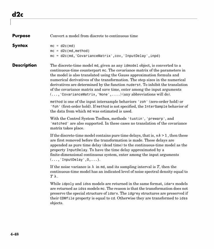
d2c
4-48
4d2cPurpose Convert a model from discrete to continuous time
Syntax mc = d2c(md)mc = d2c(md,method)mc = d2c(md,'CovarianceMatrix',cov,'InputDelay',inpd)
Description The discrete-time model md, given as any idmodel object, is converted to a continuous-time counterpart mc. The covariance matrix of the parameters in the model is also translated using the Gauss approximation formula and numerical derivatives of the transformation. The step sizes in the numerical derivatives are determined by the function nuderst. To inhibit the translation of the covariance matrix and save time, enter among the input arguments (...,'CovarianceMatrix,'None',....) (any abbreviations will do).
method is one of the input intersample behaviors 'zoh' (zero-order hold) or 'foh' (first-order hold). If method is not specified, the InterSample behavior of the data from which md was estimated is used.
With the Control System Toolbox, methods 'tustin', 'prewarp', and 'matched' are also supported. In these cases no translation of the covariance matrix takes place.
If the discrete-time model contains pure time delays, that is, , then these are first removed before the transformation is made. These delays are appended as pure time delay (dead time) to the continuous-time model as the property InputDelay. To have the time delay approximated by a finite-dimensional continuous system, enter among the input arguments (...,'InputDelay',0,...).
If the noise variance is in md, and its sampling interval is T, then the continuous-time model has an indicated level of noise spectral density equal to T .
While idpoly and idss models are returned in the same format, idarx models are returned as idss models mc. The reason is that the transformation does not preserve the special structure of idarx. The idgrey structures are preserved if their CDMfile property is equal to cd. Otherwise they are transformed to idss objects.
nk 1>
λ
λ
d2c
4-49
Note The transformation from discrete to continuous time is not unique. d2c selects the continuous-time counterpart with the slowest time constants consistent with the discrete-time model. The lack of uniqueness also means that the transformation can be ill-conditioned or even singular. In particular, poles on the negative real axis, in the origin, or in the point 1, are likely to cause problems. Interpret the results with care.
Examples Transform an identified model to continuous time and compare the frequency responses of the two models.
m = n4sid(data,3)mc = d2c(m);bode(m.mc,'sd',3)
Note that you can include the transformation to continuous time in the n4sid command by specifying the model to be continuous time.
mc = n4sid(data,3,'Ts',0)
See Also c2d, nuderst
References See “Discrete- and Continuous-Time Models” on page 3-68 and “Spectrum Normalization and the Sampling Interval” on page 3-103.
EstimationInfo
4-50
4EstimationInfoPurpose Provide information about the results of the estimation process
Syntax m.EstimationInfom.esm.es.DataLength, etc
Description Any estimated model has the property EstimationInfo, which is a structure whose fields give information about the results of the estimation. Depending on whether it is an estimated parametric idmodel or an estimated frequency response idfrd, EstimationInfo will contain different fields.
idmodel CaseThe model structure will contain the properties ParameterVector, CovarianceMatrix, and NoiseVariance, which are all calculated in the estimation process (see the reference page for idmodel). In addition, EstimationInfo contains the following fields:
• Status: Information whether the model has been estimated, or modified after being estimated.
• Method: Name of the estimation command that produced the model.
• LossFcn: Value of the identification criterion at the estimate. Normally equal to the determinant of the covariance matrix of the prediction errors, that is, the determinant of NoiseVariance. Note that the loss function for the minimization might be different due to LimitError. The value of the nonrobustified loss function is always stored in LossFcn.
• FPE: Akaike’s Final Prediction Error, defined as LossFcn *(1+d/N}/(1-d/N), where d is the number of estimated parameters and N is the length of the data record.
• DataName: Name of the data set from which the model was estimated. This is equal to the property name of the iddata object. If this was not defined, the name of the MATLAB iddata variable is used.
• DataLength: Length of the data record.
• DataTs: Sampling interval of the data.
• DataDomain: 'Time' or 'Frequency', depending on the data domain.
EstimationInfo
4-51
• DataInterSample: Intersample behavior of the data from which the model was estimated. This equals the property InterSample of the iddata object. (See iddata.)
• WhyStop: For models that have been estimated by iterative search. The stopping rule that caused the iterations to terminate. Assumes values like 'MaxIter reached', 'No improvement possible along the search vector', or 'Near (local) minimum'. The latter means that the expected improvement is less than Tolerance (see Algorithm Properties).
• UpdateNorm: Norm of the Gauss-Newton vector at the last iteration.
• LastImprovement: Relative improvement of the criterion value at the last iteration.
• Iterations: Number of iterations used in the search.
• InitialState: Option actually used when Model.InitialState = 'auto'.
• N4Weight: For n4sid estimates, or estimates that have been initialized by n4sid: the actual value of N4Weight used.
• N4Horizon: For n4sid estimates, or estimates that have been initialized by n4sid: the actual value of N4Horizon used. See n4sid and Algorithm Properties.
idfrd CaseIf the idfrd model is obtained from an estimated parametric model,
g = idfrd(Model)
g.EstimationInfo is the same as Model.EstimationInfo as described above.
For an idfrd model that has been estimated from etfe, spa, or spafdr, EstimationInfo contains the following fields:
• Status: Whether the model is estimated or directly constructed.
• Method: etfe, spa, or spafdr
• WindowSize: Resolution parameter (or vector) used for the estimation
• DataName, DataLength, DataTs, DataDomain, DataInterSample: Properties of the estimation data as above.
See Also idfrd, idmodel

etfe
4-52
4etfePurpose Estimate empirical transfer functions and periodograms
Syntax g = etfe(data)g = etfe(data,M,N)
Description etfe estimates the transfer function g of the general linear model
data contains the output-input data and is an iddata object (time or frequency domain).
g is given as an idfrd object with the estimate of at the frequencies
w = [1:N]/N∗ pi/T
The default value of N is 128.
In case data contains a time series (no input channels), g is returned as the periodogram of y.
When M is specified other than the default value M = [], a smoothing operation is performed on the raw spectral estimates. The effect of M is then similar to the effect of M in spa. This can be a useful alternative to spa for narrowband spectra and systems, which require large values of M.
When etfe is applied to time series, the corresponding spectral estimate is normalized in the way that is defined in “Spectrum Normalization and the Sampling Interval” on page 3-103. Note that this normalization might differ from the one used by spectrum in the Signal Processing Toolbox.
If the (input) data is marked as periodic (data.Period = integer) and contains an even number of periods, the response is computed at the frequencies k*2*pi/period for k = 0 up to the Nyquist frequency.
Examples Compare an empirical transfer function estimate to a smoothed spectral estimate.
ge = etfe(z);gs = spa(z);bode(ge,gs)
y t( ) G q( )u t( ) v t( )+=
G eiω( )
etfe
4-53
Generate a periodic input, simulate a system with it, and compare the frequency response of the estimated model with the true system at the excited frequency points.
m = idpoly([1 -1.5 0.7],[0 1 0.5]);u = iddata([],idinput([50,1,10],'sine'));u.Period = 50;y = sim(m,u);me = etfe([y u])bode(me,'b*',m)
Algorithm The empirical transfer function estimate is computed as the ratio of the output Fourier transform to the input Fourier transform, using fft. The periodogram is computed as the normalized absolute square of the Fourier transform of the time series.
You obtain the smoothed versions (M less than the length of z) by applying a Hamming window to the output fast Fourier transform (FFT) times the conjugate of the input FFT, and to the absolute square of the input FFT, respectively, and subsequently forming the ratio of the results. The length of this Hamming window is equal to the number of data points in z divided by M, plus one.
See Also spa, spafdr
fcat
4-54
4fcatPurpose Concatenate frequency-domain signals in idfrd and iddata objects
Syntax Mc = fcat(M1,M2,...Mn)
Description M1, M2, etc., are all idfrd objects or iddata frequency-domain objects.
Mc is the corresponding object obtained by concatenation of the responses at all the frequencies in Mk.
Note that for iddata objects, this is the same as vertical concatenation (vertcat).
Mc = [M1;M2;..;Mn].
See Also fselect, iddata, idfrd

feedback
4-55
4feedbackPurpose Investigate feedback effects in iddata sets
Syntax [fbck,fbck0,nudir] = feedback(Data)
Description Data is an iddata set with Ny outputs and Nu inputs.
fbck is an Ny-by-Nu matrix indicating the feedback. The ky,ku entry is a measure of feedback from output ky to input ku. The value is a probability P in percent. Its interpretation is that if the hypothesis that there is no feedback from output ky to input ku were tested at the level P, it would have been rejected. An intuitive but technically incorrect way of thinking about this is to see P as “the probability of feedback.” Often only values above 90% are taken as indications of feedback. When fbck is calculated, direct dependence at lag zero between u(t) and y(t) is not regarded as a feedback effect.
fbck0: Same as fbck, but direct dependence at lag 0 between u(t) and y(t) is viewed as feedback effect.
nudir: A vector containing those input numbers that appear to have a direct effect on some outputs, that is, no delay from input to output.
See Also advice. idmodel/feedback
ffplot
4-56
4ffplotPurpose Plot frequency functions and spectra
Syntax ffplot(m)[mag,phase,w] = ffplot(m)[mag,phase,w,sdmag,sdphase] = ffplot(m)ffplot(m1,m2,m3,...,w)ffplot(m1,'PlotStyle1',m2,'PlotStyle2',...)ffplot(m1,m2,m3,..'sd',sd,'mode',mode,'ap',ap)
Description This function has exactly the same syntax as bode. The only difference is that it gives graphs with linear frequency scales and Hz as the frequency unit.
See Also bode, nyquist
fft/ifft
4-57
4fft/ifftPurpose Transform iddata objects between the time and the frequency domains
Syntax Datf = fft(Data), dat = ifft(Datf)Datf = fft(Data,N)Datf = fft(Data,N,'complex')
Description If Data is a time-domain iddata object with real-valued signals and with constant sampling interval Ts, Datf is returned as a frequency-domain iddata object with the frequency values equally distributed from frequency 0 to the Nyquist frequency. Whether the Nyquist frequency actually is included or not depends on the signal length (even or odd). Note that the FFTs are normalized by dividing each transform by the square root of the signal length. That is in order to preserve the signal power and noise level.
In the default case, the length of the transformation is determined by the signal length. A second argument N will force FFT transformations of length N, padding with zeros if the signals in Data are shorter and truncating otherwise. Thus the number of frequencies in the real signal case will be N/2 or (N+1)/2. If Data contains several experiments, N can be a row vector of corresponding length.
For real signals, the default is that Datf only contains nonnegative frequencies. For complex-valued signals, negative frequencies are also included. To enforce negative frequencies in the real case, add a last argument, 'Complex'.
ifft similarily transforms a frequency-domain iddata object to the time domain. It requires the frequencies on Datf to be equally spaced from frequency 0 to the Nyquist frequency. More exactly this means that if there are N frequencies in Datf and the time sampling interval is Ts, then
Datf.Frequency = [0:df:F], where F is pi/Ts if N is odd and F = pi/Ts*(1-1/N) if N is even.
See Also iddata, iddata/complex, iddata/realdata
freqresp
4-58
4freqrespPurpose Compute the frequency function for a model
Syntax H = freqresp(m)[H,w,covH] = freqresp(m,w)
Description m is any idmodel or idfrd object.
H = freqresp(m,w) computes the frequency response H of the idmodel model m at the frequencies specified by the vector w. These frequencies should be real and in rad/s.
If m has ny outputs and nu inputs, and w contains Nw frequencies, the output H is an ny-by-nu-by-Nw array such that H(:,:,k) gives the complex-valued response at the frequency w(k).
For a SISO model, H(:) to obtain a vector of the frequency response.
If w is not specified, a default choice is made based on the dynamics of the model.
Output Arguments[H,w,covH] = freqresp(M,w)
also returns the frequencies w and the covariance covH of the response. covH is a 5-D array where covH(ky,ku,k,:,:) is the 2-by-2 covariance matrix of the response from input ku to output ky at frequency w(k). The 1,1 element is the variance of the real part, the 2,2 element is the variance of the imaginary part, and the 1,2 and 2,1 elements are the covariance between the real and imaginary parts. squeeze(covH(ky,ku,k,:,:)) gives the covariance matrix of the corresponding response.
If m is a time series (no input channels), H is returned as the (power) spectrum of the outputs, an ny-by-ny-by-Nw array. Hence H(:,:,k) is the spectrum matrix at frequency w(k). The element H(k1,k2,k) is the cross spectrum between outputs k1 and k2 at frequency w(k). When k1 = k2, this is the real-valued power spectrum of output k1.
covH is then the covariance of the estimated spectrum H, so that covH(k1,k1,k) is the variance of the power spectrum estimate of output k1 at frequency W(k). No information about the variance of the cross spectra is normally given; that is, covH(k1,k2,k) = 0 for k1 is not equal to k2.)

freqresp
4-59
If the model m is not a time series, use freqresp(m('n')) to obtain the spectrum information of the noise (output disturbance) signals.
Note that idfrd computes the same information as freqresp, and stores it in the idfrd object.
See Also bode, idfrd, nyquist
fpe
4-60
4fpePurpose Compute the Akaike Final Prediction Error for an estimated model
Syntax fp = fpe(Model1,Model2,Model3,...)
Description Model is any estimated idmodel (idarx, idgrey, idpoly, idproc, idss).
fp is returned as a row vector containing the values of the Akaike Final Prediction Error (FPE) for the different models. This is defined as
where V is the loss function, d is the number of estimated parameters, and N is the number of estimation data.
Note that it is technically possible for FPE to become negative, if the number of estimated parameters exceeds the number of data (which could happen for models with many outputs). This is an artifact where the assumption behind the derivation that d/N is small is not valid. In such a case, it is better to use AIC.
See Also EstimationInfo, aic
References Sections 7.4 and 16.4 in Ljung (1999).
FPE V1 d N⁄+1 d N⁄–----------------------=
fselect
4-61
4fselectPurpose Select frequencies from an idfrd object
Syntax idfm = fselect(idf,index)idfm = fselect(idf,Fmin,Fmax)
Description idf is any idfrd object. index is a row vector of frequency indices, so that idfm is the idfrd object that contains the response at frequencies idf.Frequency(Index).
If Fmin and Fmax are specified, idfm contains responses at frequencies between Fmin and Fmax.
Note that the operation is the same as dat(index) for an iddata object.
Examples Select every fifth frequency:
idfm = fselect(idf,5:5:100)
Select the response in the third quadrant:
ph = angle(squeeze(idf.response));idfm = fselect(idf,find(ph>-pi & ph <-pi/2))
See Also fcat
get
4-62
4getPurpose Access/query idmodel, idfrd, and iddata properties
Syntax Value = get(m,'PropertyName')get(m)Struct = get(m)
Description value = get(m,'PropertyName') returns the current value of the property PropertyName of the iddata set or idfrd, or idmodel (idgrey, idarx, idpoly, idss) m. The string 'PropertyName' can be the full property name (for example, 'SSParameterization') or any unambiguous case-insensitive abbreviation (for example, 'ss'). You can specify any generic idmodel property or any property specific to idgrey, idarx, etc. (see iddata, idmodel, idgrey, idarx, idpoly, idss, and Algorithm Properties for lists of properties that can be accessed directly).
Struct = get(m) converts the object m into a standard MATLAB structure with the property names as field names and the property values as field values.
Without a left-hand argument
get(m)
displays all properties of m and their values.
Remarks An alternative to the syntax
Value = get(m,'PropertyName')
is the structure-like referencing
Value = m.PropertyName
See Also arxdata, iddata, idfrd, idmodel, polydata, set, ssdata, tfdata, zpkdata, Algorithm Properties, EstimationInfo
getexp
4-63
4getexpPurpose Retrieve separate experiment(s) from multiple-experiment iddata objects
Syntax d1 = getexp(data,ExperimentNumber)d1 = getexp(data,ExperimentName)
Description data is an iddata object that contains several experiments. d1 is another iddata object containing the indicated experiment(s). The reference can either be by ExperimentNumber, as in d1 = getexp(data,3) or d1 = getexp(data,[4 2]); or by ExperimentName, as in d1 = getexp(data,'Period1') or d1 = getexp(data,{'Day1','Day3'}).
See merge (iddata) and iddata for how to create multiple-experiment data objects.
You can also retrieve the experiments using a fourth subscript, as in d1 = data(:,:,:,ExperimentNumber). Type help iddata/subsref for details on this.
idarx
4-64
4idarxPurpose Construct idarx model from ARX polynomials
Syntax m = idarx(A,B,Ts)m = idarx(A,B,Ts,'Property1',Value1,...,,'PropertyN',ValueN)
Description idarx creates an object containing parameters that describe the general multiinput, multioutput model structure of ARX type.
Here and are matrices of dimensions ny-by-ny and ny-by-nu, respectively. (ny is the number of outputs, that is, the dimension of the vector
, and nu is the number of inputs.) See “Multivariable ARX Models: the idarx Model” on page 3-43.
The arguments A and B are 3-D arrays that contain the A matrices and the B matrices of the model in the following way.
A is an ny-by-ny-by-(na+1) array such that
A(:,:,k+1) = AkA(:,:,1) = eye(ny)
Similarly B is an ny-by-nu-by-(nb+1) array with
B(:,:,k+1) = Bk
Note that A always starts with the identity matrix, and that delays in the model are defined by setting the corresponding leading entries in B to zero. For a multivariate time series take B = [].
The optional property NoiseVariance sets the covariance matrix of the driving noise source in the model above. The default value is the identity matrix.
The argument Ts is the sampling interval. Note that continuous-time models (Ts = 0) are not supported.
The use of idarx is twofold. You can use it to create models that are simulated (using sim) or analyzed (using bode, pzmap, etc.). You can also use it to define initial value models that are further adjusted to data (using arx). The free
y t( ) A1y t 1–( ) A2y t 2–( ) … Anay t na–( )+ + + + =
B0u t( ) B1u t 1–( ) … Bnbu t nb–( ) e t( )+ + + +
Ak Bk
y t( )
e t( )
idarx
4-65
parameters in the structure are consistent with the structure of A and B; that is, leading zeros in the rows of B are regarded as fixed delays, and trailing zeros in A and B are regarded as a definition of lower-order polynomials. These zeros are fixed, while all other parameters are free.
For a model with one output, ARX models can be described both as idarx and idpoly models. The internal representation is different, however.
idarx Properties
• A, B: The A and B polynomials as 3-D arrays, described above
• dA, dB: The standard deviations of A and B. Same format as A and B. Cannot be set.
• na, nb, nk: The orders and delays of the model. na is an ny-by-ny matrix whose i-j entry is the order of the polynomial corresponding to the i-j entry of A. Similarly nb is an ny-by-nu matrix with the orders of B. nk is also an ny-by-nu matrix, whose i-j entry is the delay from input j to output i, that is, the number of leading zeros in the i-j entry of B.
• InitialState: This describes how the initial state (initial values in filtering, etc.) should be handled. For time-domain applications, this is typically handled by starting the filtering when all data are available. For frequency-domain data, though, this requires more attention. See “Initial States for Frequency Domain Data” on page 3-99. The possible values of InitialState are 'zero', 'estimate', and 'auto' (which makes a data-dependent choice between zero and estimate).
In addition to these properties, idarx objects also have all the properties of the idmodel object. See idmodel, Algorithm Properties, and EstimationInfo.
Note that you can set and retrieve all properties either with the set and get commands or by subscripts. Autofill applies to all properties and values, and they are case insensitive.
For a complete list of property values, use get(m). To see possible value assignments, use set(m). See also idprops idarx.

idarx
4-66
Examples Simulate a second-order ARX model with one input and two outputs, and then estimate a model using the simulated data.
A = zeros(2,2,3);B = zeros(2,1,3)A(:,:,1) =eye(2);A(:,:,2) = [-1.5 0.1;-0.2 1.5];A(:,:,3) = [0.7 -0.3;0.1 0.7];B(:,:,2) = [1;-1];B(:,:,3) = [0.5;1.2];m0 = idarx(A,B,1);u = iddata([],idinput(300));e = iddata([],randn(300,2));y = sim(m0,[u e]);m = arx([y u],[[2 2;2 2],[2;2],[1;1]]);
See Also arx, arxdata, idmodel, idpoly
iddata
4-67
4iddataPurpose Package input-output data into the iddata object
Syntax data = iddata(y,u)data = iddata(y,u,Ts,'Property1',Value1,...,'PropertyN',ValueN)data = iddata(y,u,'Frequency',W)data = iddata(idfrd_object)
Description iddata is the basic object for dealing with signals in the toolbox. It is used by most of the commands. It can handle both time- and frequency-domain data. Most estimation and simulation commands can be applied to iddata objects in a transparent manner, regardless of the signal domain.
Basic UseLet y be a column vector or an N-by-ny matrix. The columns of y correspond to the different output channels. Similarly, u is a column vector or an N-by-nu matrix containing the signals of the input channels. For time-domain signals,
data = iddata(y,u,Ts)
creates an iddata object containing these output and input channels. Ts is the sampling interval. This construction is sufficient for most purposes. For frequency-domain data, the vector of frequencies W (length N) at which the signals are defined must be supplied.
data = iddata(y,u,'Frequency',W)
The data is then plotted by plot(data) (see plot), and portions of the data record are selected, as in ze = data(1:300) or zv = data(501:700).
An idfrd object can be transformed to a frequency-domain iddata object by
data = iddata(idfrd_object)
See “Transformations” on page 4-73.
The signals in the output channels are retrieved by data.OutputData, or for short, data.y. Similarly the input signals are obtained by data.InputData or data.u.
For a time series (no input channels), use data = iddata(y), or let u = [].
An iddata object can also contain just an input, if you let y = [].
iddata
4-68
The sampling interval can be changed by set(data,'Ts',0.3) or, more simply, by data.Ts = 0.3.
The input and output channels are given default names like 'y1', 'y2', 'u1','u2', etc. You can set the channel names by
set(data,'InputName',{'Voltage','Current'},'OutputName','Temperature')
(two inputs and one output in this example), and these names will then follow the object and appear in all plots. The names are also inherited by models that are estimated from the data.
Similarly, you can specify channel units using the properties 'OutputUnit' and 'InputUnit'. These units, when specified, are used in plots.
The time points associated with the time-domain data samples are determined by the sampling interval Ts and the time of the first sample, Tstart.
data.Tstart = 24
The actual time point values are given by the property 'SamplingInstants' as in
plot(data.sa,data.u)
for a plot of the input with correct time points. Autofill is used for all properties, and they are case insensitive. For frequency-domain data, the property 'Frequency' picks out the frequency values.
plot(data.fre,abs(data.u))
Manipulating ChannelsAn easy way to set and retrieve channel properties is to use subscripting. The subscripts are defined as
data(Samples,Outputs,Inputs)
so dat(:,3,:) is the data object obtained from dat by keeping all input channels, but only output channel 3. (Trailing “:”s can be omitted, so dat(:,3,:) = dat(:,3).)
The channels can also be retrieved by their names, so that
dat(:,{'speed','flow'},[])
iddata
4-69
is the data object where the indicated output channels have been selected and no input channels are selected.
Moreover,
dat1(101:200,[3 4],[1 3]) = dat2(1001:1100,[1 2],[6 7])
will change samples 101 to 200 of output channels 3 and 4 and input channels 1 and 3 in the iddata object dat1 to the indicated values from iddata object dat2. The names and units of these channels are also changed accordingly.
To add new channels, use horizontal concatenation of iddata objects.
dat =[dat1, dat2];
(see “Horizontal Concatenation” on page 4-73) or add the data record directly. Thus
dat.u(:,5) = U
adds a fifth input to dat.
Nonequal Sampling for Time-Domain DataThe property 'SamplingInstants' gives the sampling instants of the data points. It can always be retrieved by get(dat,'SamplingInstants') (or dat.s) and is then computed from dat.Ts and dat.Tstart. 'SamplingInstants' can also be set to an arbitrary vector of the same length as the data, so that nonequal sampling can be handled. Ts is then automatically set to []. Most of the estimation routines, though, do not handle unequally sampled data.
Multiple ExperimentsThe iddata object can also store data from separate experiments. The property 'ExperimentName' is used to separate the experiments. The number of data as well as the sampling properties can vary from experiment to experiment, but the input and output channels must be the same. (Use NaN to fill possibly unmeasured channels in certain experiments.) The data records will be cell arrays, where the cells contain data from each experiment.
You can define multiple experiments directly by letting the 'y' and 'u' properties, as well as 'Ts' and 'Tstart', be cell arrays. (For frequency-domain data, the frequency vector will be a cell array.)

iddata
4-70
It is normally easier to create multiple-experiment data by merging experiments, as in
dat = merge(dat1,dat2)
See the reference page for merge (data). Storing multiple experiments as one iddata object can be very useful to handle experimental data that has been collected on different occasions, or when a data set has been split up to remove “bad” portions of the data. All the toolbox’s routines accept multiple-experiment data.
Experiments can be retrieved by the command getexp. They can also be retrieved by subscripting with a fourth index: dat(:,:,:,3) is experiment #3, and dat(:,:,:,{'Day1','Day4'}) retrieves the two experiments with the indicated names.
The subscripting can be combined: dat(1:100,[2,3],[4:8],3) gives the 100 first samples of output channels 2 and 3 and input channels 4 to 8 of experiment #3. It can also be used for subassignment:
dat(:,:,:,'Run4') = dat2
which adds the data in dat2 as a new experiment with name 'Run4'. See iddemo #8 for an illustration of how multiple experiments can be used.
iddata Properties
In the list below, N denotes the number of samples of the signals, ny the number of output channels, nu the number of input channels, and Ne the number of experiments.
• Domain: Assumes the value 'Time' or 'Frequency' and denotes whether the data are time-domain or frequency-domain data.
• Name: An optional name for the data set. An arbitrary string.
• OutputData, InputData: The data matrices y and u. In the single-experiment case, y is an N-by-ny matrix and u is an N-by-nu matrix. For multiple experiments, y and u are 1-by-Ne cell arrays, with each cell containing the data for the different experiments.
• OutputName, InputName: Cell arrays of length ny-by-1 and nu-by-1 containing the names of the output and input channels. If not specified, default names {'y1';'y2';...} and {'u1';'u2';...} are given.
iddata
4-71
• OutputUnit, InputUnit: Cell arrays of length ny-by-1 and nu-by-1 containing the units of the output and input channels.
• TimeUnit: The unit for the sampling instants.
• Ts: Sampling interval. A scalar. For multiple-experiment data, Ts is a 1-by-Ne cell array, with each cell containing the sampling interval of the corresponding experiment. For nonequally sampled data, Ts = []. For time-domain signals, Ts has to be positive. For frequency-domain data, Ts = 0 indicates continuous-time data; that is, the inputs and outputs are interpreted as continuous-time Fourier transforms of the signals, given at the frequencies in the frequency vector. Note that Ts is essential also for frequency-domain data, for proper interpretation of how the Fourier transforms were computed: They are interpreted as discrete-time Fourier transforms (DTFT) with the indicated sampling interval.
• Tstart: (For time-domain data only.) The starting time of the data record. A scalar. For multiple-experiment data, Tstart is a 1-by-Ne cell array, with each cell containing the starting time for the corresponding experiment.
• SamplingInstants: (For time-domain data only.) The time values of the sample points. An N-by-1 vector. For multiple-experiment data, SamplingInstants is a 1-by-Ne cell array, with each cell containing the sampling instants of the corresponding experiment. For equally sampled data, SamplingInstants is generated from Ts and Tstart.
• Frequency: (For frequency-domain data only.) The vector of frequencies at which the signals’ transforms are defined. This is a column vector the length of the number of values of OutputData and InputData. For multiple-experiment data, Frequency is a cell array containing the frequencies for each experiment.
• Units: (For frequency-domain data only). The unit in which the frequencies are measured: rad/s or Hz. For multiple-experiment data, units is a cell array denoting the unit for each experiment.
• Period: The period of the input. A nu-by-1 vector, where the kth entry contains the period of the kth input. Period = inf means nonperiodic data. For multiple-experiment data, Period is a 1-by-Ne cell array with each cell containing the period(s) for the input of the corresponding experiment.
• InterSample: Describes the intersample behavior of the input channels. An nu-by-1 cell array where the (k,1) element is 'zoh', 'foh', or 'bl', denoting
iddata
4-72
that input number k is piecewise constant, piecewise linear, or band limited. For multiple-experiment data, InterSample is an nu-by-Ne cell array.
• ExperimentName: A string containing the name of the experiment. For multiple-experiment data, ExperimentName is a 1-by-Ne cell array with each cell containing the name of the corresponding experiment. It can be freely set, and is given names {'Exp1', 'Exp2',...} by default.
• Notes: An arbitrary field to store extra information and notes about the object.
• UserData: An arbitrary field for any possible use.
Note that you can set or retrieve all properties either with the set and get commands or by subscripts. Autofill applies to all properties and values, and they are case insensitive. 'y' and 'u' can be used as short for 'OutputData' and 'InputData'. 'y' and 'u' can also replace 'Output' and 'Input' in the other properties.
data.y=randn(100,2)data.una = 'Voltage'set(data,'tim','minute')p = data.per
For a complete list of property values, use get(data). To see possible value assignments, use set(data).
Subreferencing The samples, outputs and input channels can be referenced according to
data(samples,outputs,inputs)
Use a colon (:) to denote all samples/channels and the empty matrix ([]) to denote no samples/channels. For frequency-domain data, samples corresponds to the frequency vector indices, so that
dat2 = datf([5:30])
picks out the data values at frequencies W(5:30), where W = datf.Frequency.
The channels can be referenced by number or by name. For several names, you must use a cell array.
dat2 = dat(:,'y3',{'u1','u4'})dat2 = dat(:,3,[1 4])
iddata
4-73
Logical expressions will also work.
dat3 = dat2(dat2.sa>1.27&dat2.sa<9.3)
will select the samples with time marks between 1.27 and 9.3.
Subreferencing with a fourth argument refers to the experiment.
data(samples,outputs,inputs,Experiment)
Any subreferenced variable can also be assigned.
data(:,:,:,'Exp3'.y = flow(1:700,:)
data(1:10,1,1) = dat1(101:110,2,3)
Horizontal Concatenation
dat = [dat1,dat2,...,datN]creates an iddata object dat, consisting of the input and output channels in dat1,... datN. Default channel names ('u1', 'u2', 'y1', 'y2', etc.) are changed so that overlaps in names are avoided, and the new channels are added.
If datk contains channels with user-specified names that are already present in the channels of Datj, j<k, these new channels are ignored.
Vertical Concatenation
dat = [dat1;dat2;... ;datN] creates an iddata object dat whose signals are obtained by stacking those of datk on top of each other. That is,
dat.OutputData = [dat1.Ouputdata;dat2.OutputData; ... datN.OutputData]
and similarly for the inputs. The datk objects must all have the same number of channels and experiments.
Transforma-tions
The command fft transforms a time-domain data set to frequency domain. The command ifft transforms a frequency-domain data set (with certain requirements on the frequency vector) to time domain.
An idfrd (frequency-response data) object can be transformed to a frequency-domain iddata object by
datf = iddata(idfrdobj)
The command
datf = iddata(idfrdobj,'me')
iddata
4-74
transforms the idfrd object to a multiple-experiment data set datf where each experiment corresponds to each of the inputs in idfrdobj. By default this transformation strips away frequencies where the response is inf or NaN. To keep these, use datf = iddata(idfrdobj,'inf'). Type help idfrd/iddata.
Dealing with Complex-Valued Data
If Dat is complex valued, abs(Dat), real(Dat), imag(Dat), phase(Dat), angle(Dat), and unwrap(Dat) create iddata objects where each of the signals has been subjected to the indicated operation.
isreal(Dat) returns 1 if Dat contains only real signals, while realdata(Dat) returns 1 if the underlying signal is real. Thus a frequency-domain signal Datf obtained by fft from a real-valued time-domain signal will have
isreal(Datf) = 0 and realdata(Datf) = 1
For a realdata frequency-domain set (which only stores the values for nonnegative frequencies), the command
datc = complex(dat)
adds signal values for negative frequencies (by complex conjugation).
Online Help Functions
See help iddata, idprops iddata, help iddata/subsref, help iddata/subsasgn, help iddata/horzcat, and help iddata/vertcat.
See Also plot (iddata), size, fft, ifft, detrend, idfilt

ident
4-75
4identPurpose Open the graphical user interface
Syntax identident(session,directory)
Description ident by itself opens the main interface window, or brings it forward if it is already open.
session is the name of a previous session with the graphical user interface, and typically has extension .sid. The directory argument is the complete path for the location of this file. If the session file is on the MATLABPATH, directory can be omitted.
When the session is specified, the interface will open with this session active. Typing ident(session,directory) on the MATLAB command line, when the interface is active, will load and open the session in question.
For more information about the graphical user interface, see Chapter 2, “The Graphical User Interface.”
Examples ident('iddata1.sid')ident('mydata.sid','\matlab\data\cdplayer\')
See Also midprefs

idfilt
4-76
4idfiltPurpose Filter data using user-defined passbands or general filters or Butterworth filters
Syntax Zf = idfilt(Z,filter)Zf = idfilt(Z,filter,causality)Zf = odfilt(Z,filter,'FilterOrder',NF)
Description Z is the data, defined as an iddata object. Zf contains the filtered data as an iddata object. The filter can be defined in three ways:
• As an explicit system that defines the filter,
filter = idm or filter = {num,den} or filter = {A,B,C,D}
idm can be any SISO idmodel or LTI model object. Alternatively the filter can be defined as a cell array {A,B,C,D} of SISO state-space matrices or as a cell array {num,den} of numerator/denominator filter coefficients.
• As a vector or matrix that defines one or several passbands,
filter=[[wp1l,wp1h];[ wp2l,wp2h]; ....;[wpnl,wpnh]]
The matrix is n-by-2, where each row defines a passband in rad/s. A filter is constructed that gives the union of these passbands. For time-domain data, it is computed as cascaded Butterworth filters or order NF. The default value of NF is 5.
For example, to define a stopband between ws1 and ws2, use
filter = [0 ws1; ws2,Nyqf]
where Nyqf is the Nyquist frequency.
• For frequency-domain data, only the frequency response of the filter can be specified:
filter = Wf
Here Wf is a vector of possibly complex values that define the filter’s frequency response, so that the inputs and outputs at frequency Z.Frequency(kf) are multiplied by Wf(kf). Wf is a column vector of length = number of frequencies in Z. If the data object has several experiments, Wf is a cell array of length = # of experiments in Z.
idfilt
4-77
For time-domain data, the filtering is carried out in the time domain as causal filtering as default. This corresponds to a last argument causality = 'causal'. With causality = 'noncausal', a noncausal, zero-phase filter is used for the filtering (corresponding to filtfilt in the Signal Processing Toolbox).
For frequency-domain data, the signals are multiplied by the frequency response of the filter. With the filters defined as passband, this gives ideal, zero-phase filtering (“brickwall filters”).
It is common practice in identification to select a frequency band where the fit between model and data is concentrated. Often this corresponds to bandpass filtering with a passband over the interesting breakpoints in a Bode diagram. For identification where a disturbance model is also estimated, it is better to achieve the desired estimation result by using the property 'Focus' (see Algorithm Properties) than just to prefilter the data. The proper values for 'Focus' are the same as the argument filter in idfilt.
Algorithm The Butterworth filter is the same as butter in the Signal Processing Toolbox. Also, the zero-phase filter is equivalent to filtfilt in that toolbox.
References Ljung (1999), Chapter 14.
See Also Algorithm Properties, idresamp, detrend
idfrd
4-78
4idfrdPurpose Create the idfrd (identified frequency-response data) object that stores frequency function and spectrum data along with covariance information
Syntax h = idfrd(Response,Freqs,Ts)h = idfrd(Response,Freqs,Ts,'CovarianceData',Covariance, ...
'SpectrumData',Spec,'NoiseCovariance',Speccov,'property1', ... Value1,'PropertyN',ValueN)
h = idfrd(mod)h = idfrd(mod,Freqs)
Description idfrd creates the idfrd model object.
For a model
stores the transfer function estimate G (see (Equation 3-4) in Chapter 3, “Tutorial,”)
as well as the spectrum of the additive noise ( ) at the output
where is the estimated variance of e(t), and T is the sampling interval.
Creating idfrd from Given ResponsesResponse is a 3-D array of dimension ny-by-nu-by-Nf, with ny being the number of outputs, nu the number of inputs, and Nf the number of frequencies (that is, the length of Freqs). Response(ky,ku,kf) is thus the complex-valued frequency response from input ku to output ky at frequency =Freqs(kf). When defining the response of a SISO system, Response can be given as a vector.
Freqs is a column vector of length Nf containing the frequencies of the response.
Ts is the sampling interval. T = 0 means a continuous-time model.
y t( ) G q( )u t( ) H q( )e t( )+=
G eiω( )
Φv
Φv ω( ) λT H eiωT( )2
=
λ
ω
idfrd
4-79
Covariance is a 5-D array containing the covariance of the frequency response. It has dimension ny-by-nu-by-Nf-by-2-by-2. The structure is such that Covariance(ky,ku,kf,:,:) is the 2-by-2 covariance matrix of the response Response(ky,ku,kf). The 1-1 element is the variance of the real part, the 2-2 element is the variance of the imaginary part, and the 1-2 and 2-1 elements are the covariance between the real and imaginary parts. squeeze(Covariance(ky,ku,kf,:,:)) thus gives the covariance matrix of the corresponding response.
The information about spectrum is optional. The format is as follows:
spec is a 3-D array of dimension ny-by-ny-by-Nf, such that spec(ky1,ky2,kf) is the cross spectrum between the noise at output ky1 and the noise at output ky2, at frequency Freqs(kf). When ky1 = ky2 the (power) spectrum of the noise at output ky1 is thus obtained. For a single-output model, spec can be given as a vector.
speccov is a 3-D array of dimension ny-by-ny-by-Nf, such that speccov(ky1,ky1,kf) is the variance of the corresponding power spectrum. Normally, no information is included about the covariance of the nondiagonal spectrum elements.
If only SpectrumData is to be packaged in the idfrd object, set Response = [].
Creating idfrd from a Given Modelidfrd can also be computed from a given model mod (defined as any idmodel object).
If the frequencies Freqs are not specified, a default choice is made based on the dynamics of the model mod.
If mod has InputDelay different from zero, these are appended as phase lags, and h will then have an InputDelay of 0.
The estimated covariances are computed using the Gauss approximation formula from the uncertainty information in mod. For models with complicated parameter dependencies, numerical differentiation is applied. The step sizes for the numerical derivatives are determined by nuderst.
Frequency responses for submodels can be obtained by the standard subreferencing, h = idfrd(m(2,3)). See idmodel. In particular, h = idfrf(m('measured')) gives an h that just contains the ResponseData
idfrd
4-80
(G) and no spectra. Also h = idfrd(m('noise')) gives an h that just contains SpectrumData.
The idfrd models can be graphed with bode, ffplot, and nyquist, which all accept mixtures of idmodel and idfrd models as arguments. Note that spa, spafdr, and etfe return their estimation results as idfrd objects.
idfrd Properties
• ResponseData: 3-D array of the complex-valued frequency response as described above. For SISO systems use Response(1,1,:) to obtain a vector of the response data.
• Frequency: Column vector containing the frequencies aT which the responses are defined.
• CovarianceData: 5-D array of the covariance matrices of the response data as described above.
• SpectrumData: 3-D array containing power spectra and cross spectra of the output disturbances (noise) of the system.
• NoiseCovariance: 3-D array containing the variances of the power spectra, as explained above.
• Units: Unit of the frequency vector. Can assume the values 'rad/s' and 'Hz'.
• Ts: Scalar denoting the sampling interval of the model whose frequency response is stored. 'Ts' = 0 means a continuous-time model.
• Name: An optional name for the object.
• InputName: String or cell array containing the names of the input channels. It has as many entries as there are input channels.
• OutputName: Correspondingly for the output channels.
• InputUnit: Units in which the input channels are measured. It has the same format as 'InputName'.
• OutputUnit: Correspondingly for the output channels.
• InputDelay: Row vector of length equal to the number of input channels. Contains the delays from the input channels. These should thus be appended as phase lags when the response is calculated. This is done automatically by freqresp, bode, ffplot, and nyquist. Note that if the idfrd is calculated from an idmodel, possible input delays in that model are converted to phase lags, and the InputDelay of the idfrd model is set to zero.
idfrd
4-81
• Notes: An arbitrary field to store extra information and notes about the object.
• UserData: An arbitrary field for any possible use.
• EstimationInfo: Structure that contains information about the estimation process that is behind the frequency data. It contains the following fields (see also the reference page for EstimationInfo).
- Status: Gives the status of the model, for example, 'Not estimated'.
- Method: The identification routine that created the model.
- WindowSize: If the model was estimated by spa, spafdr, or etfe, the size of window (input argument M, the resolution parameter) that was used. This is scalar or a vector.
- DataName: Name of the data set from which the model was estimated.
- DataLength: Length of this data set.
Note that you can set or retrieve all properties either with the set and get commands or by subscripts. Autofill applies to all properties and values, and these are case insensitive:
h.ts = 0loglog(h.fre,squeeze(h.spe(2,2,:)))
For a complete list of property values, use get(m). To see possible value assignments, use set(m). See also idprops idfrd.
Subreferencing The different channels of the idfrd are retrieved by subreferencing.
h(outputs,inputs)
h(2,3) thus contains the response data from input channel 3 to output channel 2, and, if applicable, the output spectrum data for output channel 2. The channels can also be referred to by their names, as in h('power',{'voltage',''speed'}).
h('m')
contains the information for measured inputs only, that is, just ResponseData, while
h('n')
('n' for 'noise') just contains SpectrumData.

idfrd
4-82
Horizontal Concatenation
Adding input channels,
h = [h1,h2,...,hN]
creates an idfrd model h, with ResponseData containing all the input channels in h1,...,hN. The output channels of hk must be the same, as well as the frequency vectors. SpectrumData is ignored.
Vertical Concatenation
Adding output channels,
h = [h1;h2;... ;hN]
creates an idfrd model h with ResponseData containing all the output channels in h1, h2,...,hN. The input channels of hk must all be the same, as well as the frequency vectors. SpectrumData is also appended for the new outputs. The cross spectrum between output channels is then set to zero.
Converting to iddata
You can convert an idfrd object to a frequency-domain iddata object by
Data = iddata(Idfrdmodel)
See iddata.
Examples Compare the results from spectral analysis and an ARMAX model.
m = armax(z,[2 2 2 1]);g = spa(z)g = spafdr(z,[],{0,10})bode(g,m)
Compute separate idfrd models, one containing the frequency function and the other the noise spectrum.
g = idfrd(m('m'))phi = idfrd(m('n'))
See Also bode, etfe, freqresp, nyquist, spa
idgrey
4-83
4idgreyPurpose Package a gray-box model structure defined by a user-written M-file into an idgrey model
Syntax m = idgrey(MfileName,ParameterVector,CDmfile)m = idgrey(MfileName,ParameterVector,CDmfile,FileArgument,Ts,...'Property1',Value1,...,'PropertyN',ValueN)
Description The function idgrey is used to create arbitrarily parameterized state-space models as idgrey objects.
MfileName is the name of an M-file that defines how the state-space matrices depend on the parameters to be estimated. The format of this M-file is given by
[A,B,C,D,K,X0] = mymfile(pars,Tsm,Auxarg)
and is further discussed below.
ParameterVector is a column vector of the nominal/initial parameters. Its length must be equal to the number of free parameters in the model (that is, the argument pars in the example below).
The argument CDmfile describes how the user-written M-file handles continuous and discrete-time models. It takes the following values:
• CDmfile = 'cd': The M-file returns the continuous-time state-space matrices when called with the argument Tsm = 0. When called with a value Tsm > 0, the M-file returns the discrete-time state-space matrices, obtained by sampling the continuous-time system with sampling interval Tsm. The M-file must consequently in this case include the sampling procedure.
• CDmfile = 'c'. The M-file always returns the continuous-time state-space matrices, no matter the value of Tsm. In this case the toolbox’s estimation routines will provide the sampling when you are fitting the model to discrete-time data.
• CDmfile='d'. The M-file always returns discrete-time state-space matrices that may or may not depend on Tsm.
The argument FileArgument corresponds to the auxiliary argument Auxarg in the user-written M-file. It can be used to handle several variants of the model structure, without your having to edit the M-file. If it is not used, enter FileArgument = []. (Default.)
idgrey
4-84
Ts denotes the sampling interval of the model. Its default value is Ts = 0, that is, a continuous-time model.
The idgrey object is a child of idmodel. Therefore any idmodel properties can be set as property name/property value pairs in the idgrey command. They can also be set by the command set, or by subassignment, as in
m.InputName = {'speed','voltage'}m.FileArgument = 0.23
There are also two properties, DisturbanceModel and InitialState, that can be used to affect the parameterizations of K and X0, thus overriding the outputs from the M-file.
idgrey Properties
• MfileName: Name of the user-written M-file.
• CDmfile: How this file handles continuous and discrete-time models depending on its second argument, T.
- CDmfile = 'cd' means that the M-file returns the continuous-time state-space model matrices when the argument T = 0, and the discrete-time model, obtained by sampling with sampling interval T, when T > 0.
- CDmfile= 'c' means that the M-file always returns continuous-time model matrices, no matter the value of T.
- CDmfile = 'd' means that the M-file always returns discrete-time model matrices that may or may not depend on the value of T.
• FileArgument: Possible extra input arguments to the user-written M-file.
• DisturbanceModel: Affects the parameterization of the K matrix. It can assume the following values:
- 'Model': This is the default. It means that the K matrix obtained from the user-written M-file is used.
- 'Estimate': The K matrix is treated as unknown and all its elements are estimated as free parameters.
- 'Fixed': The K matrix is fixed to a given value.
- 'None': The K matrix is fixed to zero, thus producing an output-error model.
Note that in the three last cases the output K from the user-written M-file is ignored. The estimated/fixed value is stored internally and does not change

idgrey
4-85
when the model is sampled, resampled, or converted to continuous time. Note also that this estimated value is tailored only to the sampling interval of the data.
• InitialState: Affects the parameterization of the X0 vector. It can assume the following values:
- 'Model': This is the default. It means that the X0 vector is obtained from the user-written M-file.
- 'Estimate': The X0 matrix is treated as unknown and all its elements are estimated as free parameters.
- 'Fixed': The X0 vector is fixed to a given value.
- 'Backcast': The X0 vector is estimated using a backcast operation analogous to the idss case.
- 'Auto': Makes a data-dependent choice among 'Estimate', 'Backcast', and 'Model'.
• A, B, C, D, K, and X0: The state-space matrices. For idgrey models, only 'K' and 'X0' can be set; the others can only be retrieved. The set 'K' and 'X0' are relevant only when DisturbanceModel/InitialState are Estimate or Fixed.
• dA, dB, dC, dD, dK, and dX0: The estimated standard deviations of the state-space matrices. These cannot be set, only retrieved.
In addition, any idgrey object also has all the properties of idmodel. See Algorithm Properties and the reference page for idmodel.
Note that you can set or retrieve all properties using either the set and get commands or subscripts. Autofill applies to all properties and values, and they are case insensitive.
m.fi = 10;set(m,'search','gn')p = roots(m.a)
For a complete list of property values, use get(m). To see possible value assignments, use set(m). See also idprops and idgrey.
M-File Details The model structure corresponds to the general linear state-space structure

idgrey
4-86
Here is the time derivative for a continuous-time model and for a discrete-time model.
The matrices in this time-discrete model can be parameterized in an arbitrary way by the vector . Write the format for the M-file as follows:
[A,B,C,D,K,x0] = mymfile(pars,T,Auxarg)
Here the vector pars contains the parameters , and the output arguments A, B, C, D, K, and x0 are the matrices in the model description that correspond to this value of the parameters and this value of the sampling interval T.
T is the sampling interval, and Auxarg is any variable of auxiliary quantities with which you want to work. (In that way you can change certain constants and other aspects in the model structure without having to edit the M-file.) Note that the two arguments T and Auxarg must be included in the function head of the M-file, even if they are not used within the M-file.
“State-Space Models with Coupled Parameters: the idgrey Model” on page 3-51 contains several examples of typical M-files that define model structures.
A comment about CDmfile: If a continuous-time model is sought, it is easiest to let the M-file deliver just the continuous-time model, that is, have CDmfile = 'c' and rely upon the toolbox’s routines for the proper sampling. Similarly, if the underlying parameterization is indeed discrete time, it is natural to deliver the discrete-time model matrices and let CDmfile = 'd'. If the underlying parameterization is continuous, but you prefer for some reason to do your own sampling inside the M-file in accordance with the value of T, then let your M-file deliver the continuous-time model when called with T = 0, that is, the alternative CMmfile = 'cd'. This avoids sampling and then transforming back (using d2c) to find the continuous-time model.
Examples Use the M-file mynoise given in “Example 3.4: Parameterized Disturbance Models” on page 3-53 to obtain a physical parameterization of the Kalman gain.
x t( ) A θ( )x t( ) B θ( )u t( ) K θ( )e t( )+ +=
x 0( ) x0 θ( )=
y t( ) C θ( )x t( ) D θ( )u t( ) e t( )+ +=
x t( ) x· t( ) x t Ts+( )
θ
θ

idgrey
4-87
mn = idgrey('mynoise',[0.1,-2,1,3,0.2]','d')m = pem(z,mn)
idinput
4-88
4idinputPurpose Generate signals, typically to be used as inputs for identification
Syntax u = idinput(N)u = idinput(N,type,band,levels)[u,freqs] = idinput(N,'sine',band,levels,sinedata)
Description idinput generates input signals of different kinds, which are typically used for identification purposes. u is returned as a matrix or column vector.
For further use in the toolbox, we recommend that you create an iddata object from u, indicating sampling time, input names, periodicity, and so on:
u = iddata([],u);
N determines the number of generated input data. If N is a scalar, u is a column vector with this number of rows.
N = [N nu] gives an input with nu input channels each of length N.
N = [P nu M] gives a periodic input with nu channels, each of length M*P and periodic with period P.
Default is nu = 1 and M = 1.
type defines the type of input signal to be generated. This argument takes one of the following values:
• type = 'rgs': Gives a random, Gaussian signal.
• type = 'rbs': Gives a random, binary signal. This is the default.
• type = 'prbs': Gives a pseudorandom, binary signal.
• type = 'sine': Gives a signal that is a sum of sinusoids.
The frequency contents of the signal is determined by the argument band. For the choices type = 'rs', 'rbs', and 'sine', this argument is a row vector with two entries
band = [wlow, whigh]
that determine the lower and upper bound of the passband. The frequencies wlow and whigh are expressed in fractions of the Nyquist frequency. A white noise character input is thus obtained for band = [0 1], which is also the default value.

idinput
4-89
For the choice type = 'prbs',
band = [0, B]
where B is such that the signal is constant over intervals of length 1/B (the clock period). In this case the default is band = [0 1].
The argument levels defines the input level. It is a row vector
levels = [minu, maxu]
such that the signal u will always be between the values minu and maxu for the choices type = 'rbs', 'prbs', and 'sine'. For type = 'rgs', the signal level is such that minu is the mean value of the signal, minus one standard deviation, while maxu is the mean value plus one standard deviation. Gaussian white noise with zero mean and variance one is thus obtained for levels = [-1, 1], which is also the default value.
Some PRBS AspectsIf more than one period is demanded (that is, M > 1), the length of the data sequence and the period of the PRBS signal are adjusted so that an integer number of maximum length PRBS periods is always obtained. If M = 1, the period of the PRBS signal is chosen to that it is longer than P = N. In the multiinput case, the signals are maximally shifted. This means P/nu is an upper bound for the model orders that can be estimated with such a signal.
Some Sine AspectsIn the 'sine' case, the sinusoids are chosen from the frequency grid
freq = 2*pi*[1:Grid_Skip:fix(P/2)]/P intersected with pi*[band(1) band(2)]
(for Grid_Skip, see below.) For multiinput signals, the different inputs use different frequencies from this grid. An integer number of full periods is always delivered. The selected frequencies are obtained as the second output argument, freqs, where row ku of freqs contains the frequencies of input number ku. The resulting signal is affected by a fifth input argument, sinedata
sinedata = [No_of_Sinusoids, No_of_Trials, Grid_Skip]
idinput
4-90
meaning that No_of_Sinusoids is equally spread over the indicated band. No_of_Trials (different, random, relative phases) are tried until the lowest amplitude signal is found.
Default: sinedata = [10,10,1];
Grid_Skip can be useful for controlling odd and even frequency multiples, for example, to detect nonlinearities of various kinds.
Algorithm Very simple algorithms are used. The frequency contents are achieved for 'rgs' by an eighth-order Butterworth, noncausal filter, using idfilt. This is quite reliable. The same filter is used for the 'rbs' case, before making the signal binary. This means that the frequency contents are not guaranteed to be precise in this case.
For the 'sine' case, the frequencies are selected to be equally spread over the chosen grid, and each sinusoid is given a random phase. A number of trials are made, and the phases that give the smallest signal amplitude are selected. The amplitude is then scaled so as to satisfy the specifications of levels.
References See Söderström and Stoica (1989), Chapter C5.3. For a general discussion of input signals, see Ljung (1999), Section 13.3.
Examples Create an input consisting of five sinusoids spread over the whole frequency interval. Compare the spectrum of this signal with that of its square. The frequency splitting (the square having spectral support at other frequencies) reveals the nonlinearity involved:
u = idinput([100 1 20],'sine',[],[],[5 10 1]);u = iddata([],u,1,'per',100);u2 = u.u.^2;u2 = iddata([],u2,1,'per',100);ffplot(etfe(u),'r*',etfe(u2),'+')
idmdlsim
4-91
4idmdlsimPurpose Simulate idmodel objects in Simulink
Syntax idmdlsim
Description Typing idmdlsim launches the Idmodel block in Simulink. By clicking the block you can specify the idmodel to simulate, whether to include initial state values, and whether to add noise to the simulation in accordance with the model’s own noise description.
idmodel
4-92
4idmodel Purpose Package all common model properties
Description idmodel is an object that the user does not deal with directly. It contains all the common properties of the model objects idarx, idgrey, idpoly, idproc, and idss, which are returned by the different estimation routines.
Basic UseIf you just estimate models from data, the model objects should be transparent. All parametric estimation routines return idmodel results.
m = arx(Data,[2 2 1])
The model m contains all relevant information. Just typing m will give a brief account of the model. present(m) also gives information about the uncertainties of the estimated parameters. get(m) gives a complete list of model properties.
Most of the interesting properties can be directly accessed by subreferencing.
m.am.da
See the property list obtained by get(m), as well as the property lists of idgrey, idarx, idpoly, and idss in Chapter 4, “Function Reference,” for more details on this. See also idprops.
The characteristics of the model m can be directly examined and displayed by commands like impulse, step, bode, nyquist, and pzmap. The quality of the model is assessed by commands like compare and resid. If you have the Control System Toolbox, typing view(m) gives access to various display functions.
To extract state-space matrices, transfer function polynomials, etc., use the commands arxdata, polydata, tfdata, ssdata, and zpkdata.
To compute the frequency response of the model, use the commands idfrd and freqresp.
Creating and Modifying Model ObjectsIf you want to define a model to use, for example, for simulating data, you need to use the model creator functions:
idmodel
4-93
• idarx, for multivariable ARX models
• idgrey, for user-defined gray-box state-space models
• idpoly, for single-output polynomial models
• idproc, for simple, continuous-time process models
• idss, for state-space models
If you want to estimate a state-space model with a specific internal parameterization, you need to create an idss model or an idgrey model. See the reference pages for these functions.
Dealing with Input and Output ChannelsFor multivariable models, you construct submodels containing a subset of inputs and outputs by simple subreferencing. The outputs and input channels can be referenced according to
m(outputs,inputs)
Use a colon (:) to denote all channels and an empty matrix ([]) to denote no channels. The channels can be referenced by number or by name. For several names, you must use a cell array, such as
m3 = m('position',{'power','speed'})
or
m3 = m(3,[1 4])
Thus m3 is the model obtained from m by looking at the transfer functions from input numbers 1 and 4 (with input names 'power' and 'speed') to output number 3 (with name position).
For a single-output model m,
m4 = m(inputs)
selects the corresponding input channels, and for a single-input model,
m5 = m(outputs)
selects the indicated output channels.
Subreferencing is quite useful, for example, when a plot of just some channels is desired.
idmodel
4-94
The Noise ChannelsThe estimated models have two kinds of input channels: the measured inputs u and the noise inputs e. For a general linear model m, we have
(4-2)
where u is the nu-dimensional vector of measured input channels and e is the ny-dimensional vector of noise channels. The covariance matrix of e is given by the property 'NoiseVariance'. Occasionally this matrix is written in factored form,
This means that e can be written as
where is white noise with identity covariance matrix (independent noise sources with unit variances).
If m is a time series (nu = 0), G is empty and the model is given by
For the model m, the restriction to the transfer function matrix G is obtained by
m1 = m('measured') or just m1 = m('m')
Then e is set to 0 and H is removed.
Analogously,
m2 = m('noise') or just m2 = m('n')
creates a time-series model m2 from m by ignoring the measured input. That is, m2 describes the signal He.
For a system with measured inputs, bode, step, and other transformation and display functions deal with the transfer function matrix G. To obtain or graph the properties of the disturbance model H, it is therefore important to make the transformations m('n'). For example,
bode(m('n'))
plots the additive noise spectra according to the model m, while
y t( ) G q( )u t( ) H q( )e t( )+=
Λ
Λ LLT=
e Lv=
v
y t( ) H q( )e t( )=
idmodel
4-95
bode(m)
just plots the frequency responses of G.
To study the noise contributions in more detail, it is useful to convert the noise channels to measured channels, using the command noisecnv.
m3 = noisecnv(m)
This creates a model m3 with all input channels, both measured u and noise sources e, treated as measured signals,. That is, m3 is a model from u and e to y, describing the transfer functions G and H. The information about the variance of the innovations e is lost. For example, studying the step response from the noise channels does not take into consideration how large the noise contributions actually are.
To include that information, e should first be normalized, , so that becomes white noise with an identity covariance matrix.
m4 = noisecnv(m,'Norm')
This creates a model m4 with u and treated as measured signals.
For example, the step responses from v to y will now reflect the typical size of the disturbance influence because of the scaling by L. In both cases, the previous noise sources that have become regular inputs will automatically get input names that are related to the corresponding output. The unnormalized noise sources e have names like 'e@ynam1' (noise e at output channel ynam1), while the normalized sources v are called 'v@ynam1'.
Retrieving Transfer FunctionsThe functions that retrieve transfer function properties, ssdata, tfdata, and zpkdata, will thus work as follows for a model (Equation 4-2) with measured inputs. (fcn is ssdata, tfdata, or zpkdata.)
fcn(m) returns the properties of G (ny outputs and nu inputs).
fcn(m('n')) returns the properties of the transfer function H (ny outputs and ny inputs).
e Lv= v
v
y t( ) G q( )u t( ) H q( )Lv t( )+ G HLuv
= =
idmodel
4-96
fcn(noisec nv(m,'Norm')) returns the properties of the transfer function [G HL} (ny outputs and ny+nu inputs). Analogously,
m1 = m('n'). fcn(noisecnv(m1,'Norm'))
returns the properties of the transfer function HL (ny outputs and ny inputs).
If m is a time-series model, fcn(m) returns the properties of H, while
fcn(noisecnv(m,'Norm'))
returns the properties of HL.
Note that the estimated covariance matrix NoiseVariance itself is uncertain. This means that the uncertainty information about H is different from that of HL.
idmodel Properties
In the list below, ny is the number of output channels, and nu is the number of input channels:
• Name: An optional name for the data set. An arbitrary string.
• OutputName, InputName: Cell arrays of length ny-by-1 and nu-by-1 containing the names of the output and input channels. For estimated models, these are inherited from the data. If not specified, they are given default names {'y1','y2',...} and {'u1','u2',...}.
• OutputUnit, InputUnit: Cell arrays of length ny-by-1 and nu-by-1 containing the units of the output and input channels. Inherited from data for estimated models.
• TimeUnit: Unit for the sampling interval.
• Ts: Sampling interval. A nonnegative scalar. Ts = 0 denotes a continuous-time model. Note that changing just Ts will not recompute the model parameters. Use c2d and d2c for recomputing the model to other sampling intervals.
• ParameterVector: Vector of adjustable parameters in the model structure. Initial/nominal values or estimated values, depending on the status of the model. A column vector.
• PName: The names of the parameters. A cell array of the length of the parameter vector. If not specified, it will contain empty strings. See also setpname.
idmodel
4-97
• CovarianceMatrix: Estimated covariance matrix of the parameter vector. For a nonestimated model this is the empty matrix. For state-space models in the 'Free' parameterization the covariance matrix is also the empty matrix, since the individual matrix elements are not identifiable then. Instead, in this case, the covariance information is hidden (in the hidden property 'Utility') and retrieved by the relevant functions when necessary. Setting CovarianceMatrix to 'None' inhibits calculation of covariance and uncertainty information. This can save substantial time for certain models. See “No Covariance” on page 3-100.
• NoiseVariance: Covariance matrix of the noise source e. An ny-by-ny matrix.
• InputDelay: Vector of size nu-by-1, containing the input delay from each input channel. For a continuous-time model (Ts = 0) the delay is measured in TimeUnit, while for discrete-time models (Ts > 0) the delay is measured as the number of samples. Note the difference between InputDelay and nk (which is a property of idarx, idss, and idpoly). 'Nk' is a model structure property that tells the model structure to include such an input delay. In that case, the corresponding state-space matrices and polynomials will explicitly contain Nk input delays. The property InputDelay, on the other hand, is an indication that in addition to the model as defined, the inputs should be shifted by the given amount. InputDelay is used by sim and the estimation routines to shift the input data. When computing frequency responses, the InputDelay is also respected. Note that InputDelay can be both positive and negative.
• Algorithm: See the reference page for Algorithm Properties.
• EstimationInfo: See the reference page for EstimationInfo.
• Notes: An arbitrary field to store extra information and notes about the object.
• UserData: An arbitrary field for any possible use.
Note All properties can be set or retrieved either by these commands or by subscripts. Autofill applies to all properties and values, and is case insensitive.
For a complete list of property values, use get(m). To see possible value assignments, use set(m).
idmodel
4-98
Subreferencing The outputs and input channels can be referenced according to
m(outputs,inputs)
Use a colon (:) to denote all channels and an empty matrix ([ ]) to denote no channels. The channels can be referenced by number or by name. For several names, you must use a cell array.
m2 = m('y3',{'u1','u4'})
m3 = m(3,[1 4])
For a single output model m,
m4 = m(inputs)
selects the corresponding input channels, and for a single input model,
m5 = m(outputs)
selects the indicated output channels.
The string 'measured' (or any abbreviation like 'm') means the measured input channels.
m4 = m(3,'m')m('m') is the same as m(:,'m')
Similarly, the string 'noise' (or any abbreviation) refers to the noise input channels. See “The Noise Channels” on page 4-94 for more details.
Horizontal Concatenation
Adding input channels,
m = [m1,m2,...,mN]
creates an idmodel object m, consisting of all the input channels in m1,... mN. The output channels of mk must be the same.
Vertical Concatenation
Adding output channels,
m = [m1;m2;... ;mN]
creates an idmodel object m consisting of all the output channels in m1, m2, ..mN. The input channels of mk must all be the same.

idmodel
4-99
Online Help Functions
See idhelp. idprops idmodel, help idmodel/subsref, help idmodel/subsasgn, help idmodel/horzcat, and help idmodel/vertcat.
See Also noisecnv, nkshift, view, size, idmdlsim, sim
idmodred
4-100
4idmodredPurpose Reduce the order of a model (requires the Control System Toolbox)
Syntax MRED = idmodred(M)MRED = idmodred(M,ORDER,'DisturbanceModel','None')
Description This function reduces the order of any model M given as an idmodel object. The resulting reduced order model MRED is an idss model.
The function requires several routines in the Control System Toolbox.
ORDER: The desired order (dimension of the state-space representation). If ORDER = [], which is the default, a plot will show how the diagonal elements of the observability and controllability Gramians of a balanced realization decay with the order of the representation. You are then prompted to select an order based on this plot. The idea is that such a small element will have a negligible influence on the input-output behavior of the model. We recommend that you choose an order such that only large elements in these matrices are retained.
'DisturbanceModel': If the property DisturbanceModel is set to 'None', then an output-error model MRED is produced, that is, one with the Kalman gain equal to zero (see Equation 3-23 in “Chapter 3, “Tutorial”). Otherwise (default), the disturbance model is reduced.
The function recognizes whether M is a continuous- or discrete-time model and performs the reduction accordingly. The resulting model MRED is of the same kind in this respect as M.
Algorithm The functions balreal and modred from the Control System Toolbox are used. The plot, in case ORDER = [], shows the vector g as returned from balreal.
Examples Build a high-order multivariable ARX model, reduce its order to 3, and compare the frequency responses of the original and reduced models.
M = arx(data,[4∗ ones(3,3),4∗ ones(3,2),ones(3,2)]);MRED = idmodred(M,3);bode(M,MRED)
Use the reduced-order model as an initial condition for a third-order state-space model.
M2 = pem(data,MRED);
idpoly
4-101
4idpolyPurpose Construct an idpoly model for input-output models
Syntax m = idpoly(A,B)m = idpoly(A,B,C,D,F,NoiseVariance,Ts)m = idpoly(A,B,C,D,F,NoiseVariance,Ts,'Property1',Value1,...
'PropertyN',ValueN)
m = idpoly(mi)
Description idpoly creates a model object containing parameters that describe the general multiinput single-output model structure.
A, B, C, D, and F specify the polynomial coefficients.
For single-input systems, these are all row vectors in the standard MATLAB format.
A = [1 a1 a2 ... ana]
consequently describes
A, C, D, and F all start with 1, while B contains leading zeros to indicate the delays. See “Polynomial Representation of Transfer Functions” on page 3-11.
For multiinput systems, B and F are matrices with one row for each input.
For time series, B and F are entered as empty matrices.
B = []; F = [];
NoiseVariance is the variance of the white noise sequence , while Ts is the sampling interval.
Trailing arguments C, D, F, NoiseVariance, and Ts can be omitted, in which case they are taken as 1. (If B = [], then F is taken as [].) The property name/property value pairs can start directly after B.
Ts = 0 means that the model is a continuous-time one. Then the interpretation of the arguments is that
A q( )y t( )B1 q( )F1 q( )---------------u1 t nk1–( )= …
Bnu q( )Fnu q( )-------------------unu t nknu–( ) C q( )
D q( )-------------e t( )+ + +
A q( ) 1 a1q 1– … anaq na–+ + +=
e t( )

idpoly
4-102
A = [1 2 3 4]
corresponds to the polynomial in the Laplace variable s, and so on. For continuous-time systems, NoiseVariance indicates the level of the spectral density of the innovations. A sampled version of the model has the innovations variance NoiseVariance/Ts, where Ts is the sampling interval. The continuous-time model must have a white noise component in its disturbance description. See “Spectrum Normalization and the Sampling Interval” on page 3-103.
For discrete-time models (Ts > 0), note the following: idpoly strips any trailing zeros from the polynomials when determining the orders. It also strips leading zeros from the B polynomial to determine the delays. Keep this in mind when you use idpoly and polydata to modify earlier estimates to serve as initial conditions for estimating new structures. See “Initial Parameter Values” on page 3-97.
idpoly can also take any single-output idmodel or LTI object mi as an input argument. If an LTI system has an input group with name 'Noise', these inputs are interpreted as white noise with unit variance, and the noise model of the idpoly model is computed accordingly.
Properties • na, nb, nc, nd, nf, nk: The orders and delays of the polynomials. Integers or row vectors of integers.
• a, b, c, d, f: The polynomials, described by row vectors and matrices as detailed above.
• da, db, dc, dd, df: The estimated standard deviation of the polynomials. Cannot be set.
• InitialState: How to deal with the initial conditions that are required to compute the prediction of the output. Possible values are
- 'Estimate': The necessary initial states are estimated from data as extra parameters.
- 'Backcast': The necessary initial states are estimated by a backcasting (backward filtering) process, described in Knudsen (1994).
- 'Zero': All initial states are taken as zero.
- 'Auto': An automatic choice among the above is made, guided by the data.
In addition, any idpoly object also has all the properties of idmodel. See idmodel properties and Algorithm Properties.
s3 2s2 3s 4+ + +
idpoly
4-103
Note that you can set or retrieve all properties either with the set and get commands or by subscripts. Autofill applies to all properties and values, and these are case insensitive.
m.a=[1 -1.5 0.7];set(m,'ini','b')p = roots(m.a)
For a complete list of property values, use get(m). To see possible value assignments, use set(m). See also idprops idpoly.
Examples To create a system of ARMAX, type
A = [1 -1.5 0.7];B = [0 1 0.5];C = [1 -1 0.2];m0 = idpoly(A,B,C);
This gives a system with one delay (nk = 1).
Create the continuous-time model
Sample it with T = 0.1 and then simulate it without noise.
B=[0 1;1 3];F=[1 1 0;1 2 4]m = idpoly(1,B,1,1,F,1,0)md = c2d(m,0.1)y = sim(md,[u1 u2])
Note that the continuous-time model is automatically sampled to the sampling interval of the data, when simulated, so the above is also achieved by
u = iddata([],[u1 u2],0.1)y = sim(m,u)
See Also sim, idss
References Ljung (1999) Section 4.2 for the model structure family.
y t( ) 1s s 1+( )--------------------u1 t( ) s 3+
s2 2s 4+ +----------------------------u2 t( ) e t( )+ +=

idpoly
4-104
Knudsen, T., (1994), “A new method for estimating ARMAX models,” In Proc. 10th IFAC Symposium on System Identification, pp. 611-617, Copenhagen, Denmark, for the backcast method.
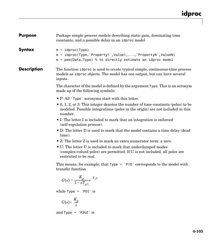
idproc
4-105
4idprocPurpose Package simple process models describing static gain, dominating time constants, and a possible delay in an idproc model
Syntax m = idproc(Type)m = idproc(Type,'Property1',Value1,...,'PropertyN',ValueN)m = pem(Data,Type) % to directly estimate an idproc model
Description The function idproc is used to create typical simple, continuous-time process models as idproc objects. The model has one output, but can have several inputs.
The character of the model is defined by the argument Type. This is an acronym made up of the following symbols:
• P: All 'Type' acronyms start with this letter.
• 0, 1, 2, or 3: This integer denotes the number of time constants (poles) to be modeled. Possible integrations (poles in the origin) are not included in this number.
• I: The letter I is included to mark that an integration is enforced (self-regulation process).
• D: The letter D is used to mark that the model contains a time delay (dead time).
• Z: The letter Z is used to mark an extra numerator term: a zero.
• U: The letter U is included to mark that underdamped modes (complex-valued poles) are permitted. If U is not included, all poles are restricted to be real.
This means, for example, that Type = 'P1D' corresponds to the model with transfer function
while Type = 'P0I' is
and Type = 'P3UZ' is
G s( )Kp
1 sTp1+----------------------e
Tds–=
G s( )Kps
-------=

idproc
4-106
For multiinput systems, Type is a cell array where each cell describes the character of the model from the corresponding input, like Type = {'P1D'.'P0I'} for the two-input model
(4-3)
The parameters of the model are
• Kp: The static gain
• Tp1, Tp2, Tp3: The real-time constants (corresponding to poles in 1/Tp1, etc.)
• Tw and Zeta: The “resonance time constant” and the damping factor corresponding to a denominator factor (1+2 Zeta Tw s + (Tw s)^2). If underdamped modes are allowed, Tw and Zeta replace Tp1 and Tp2. A third real pole, Tp3, could still be included.
• Td: The time delay
• Tz: The numerator zero
These properties contain fields that give the values of the parameters, upper and lower bounds, and information whether they are locked to zero, have a fixed value, or are to be estimated. For multiinput models, the number of entries in these fields equals the number of inputs. This is described in more detail below.
The idproc object is a child of idmodel. Therefore any idmodel properties can be set as property name/property value pairs in the idproc command. They can also be set by the command set, or by subassignment, as in
m.InputName = {'speed','voltage'}m.kp = 12
In the multiinput case, models for specific inputs can be obtained by regular subreferencing.
m(ku)
G s( ) Kp1 Tzs+
1 2ςTws Tws( )2+ +( ) 1 Tp3s+( )-------------------------------------------------------------------------------------=
Y s( )Kp 1( )
1 sTp1 1( )+-------------------------------e
Tds–U1 s( )
Kp 2( )s
---------------U2 s( )+=

idproc
4-107
There are also two properties, DisturbanceModel and InitialState, that can be used to expand the model. See below.
idproc Properties
• Type: A string or a cell array of strings with as many elements as there are inputs. The string is an acronym made up of the characters P, Z, I, U, D and an integer between 0 and 3. The string must start with P, followed by the integer, while possible other characters can follow in any order. The integer is the number of poles (not counting a possible integration), Z means the inclusion of a numerator zero, D means inclusion of a time delay, while U marks that the modes can be underdamped (a pair of complex conjugated poles). I means that an integration in the model is enforced.
• Kp, Tp1, Tp2, Tp3, Tw, Zeta, Tz, Td: These are the parameters as explained above. Each of these is a structure with the following fields:
- value: Numerical value of the parameter.
- max: Maximum allowed value of the parameter when it is estimated.
- min: Minimum allowed value of the parameter when it is estimated. For multiinput models, these are row vectors.
- status: Assumes one of 'Estimate', 'Fixed', or 'Zero'.
'Zero' means that the parameter is locked to zero and not included in the model. Assigning, for example, Type = 'P1' means that the status of Tp2, Tp3, Tw, and Zeta will be 'Zero'.
The value 'Fixed' means that the parameter is fixed to its value, and will not be estimated.
The value 'Estimate' means that the parameter value should be estimated.
For multiinput modes, status is a cell array with one element for each input, while value, max, and min are row vectors.
• DisturbanceModel: Allows an additive disturbance model as in
(4-4)
where G(s) is a process model and e(t) is white noise, and C/D is a first- or second-order transfer function.
DisturbanceModel can assume the following values:
y t( ) G s( )u t( ) C s( )D s( )------------e t( )+=
idproc
4-108
- 'None': This is the default. No disturbance model is included (that is, C=D=1).
- 'arma1': The disturbance model is a first-order ARMA model (that is, C and D are first-order polynomials).
- 'arma2' or 'Estimate': The disturbance model is a second-order ARMA model (that is, C and D are second-order polynomials).
When a disturbance model has been estimated, the property DisturbanceModel is returned as a cell array, with the first entry being the status as just defined, and the second entry being the actual model, delivered as a continuous-time idpoly object.
• InitialState: Affects the parameterization of the initial values of the states of the model. It assumes the same values as for other models:
- 'Zero': The initial states are fixed to zero.
- 'Estimate': The initial states are treated as parameters to be estimated.
- 'Backcast': The initial state vector is adjusted, during the parameter estimation step, to a suitable value, but it is not stored.
- 'Auto': Makes a data-dependent choice among the values above.
• InputLevel: The offset level of the input signal(s). This is of particular importance for those input channels that contain an integration. InputLevel will then define the level from which the integration takes place, and that cannot be handled by estimating initial states. InputLevel has the same structure as the model parameters Kp, etc., and thus contains the following fields:
- value: Numerical value of the parameter. For multiinput models, this is a row vector.
- max: Maximum allowed value of the parameter when it is estimated.
- min: Minimum allowed value of the parameter when it is estimated. For multiinput models, these are row vectors.
- status: Assumes one of 'Estimate', 'Fixed', or 'Zero' with the same interpretations.
In addition, any idproc object also has all the properties of idmodel. See Algorithm Properties, EstimationInfo, and idmodel.
Note that all properties can be set or retrieved using either the set and get commands or subscripts. Autofill applies to all properties and values, and these
idproc
4-109
are case insensitive. Also 'u' and 'y' are short for 'Input' and 'Output', respectively. You can also set all properties at estimation time as property name/property value pairs in the call to pem. An extended syntax allows direct setting of the fields of the parameter values, so that assigning a numerical value is automatically attributed to the value field, while a string is attributed to the status field.
m.kp = 10m.tp1 = 'estimate'm = pem(Data,'P1D','kp',10) % initializing the parameter Kp in 10m = pem(Data,'P1D','kp',10,'kp','fix') % fixing the parameter Kp to the value 10m.= pem(Data,'P2U','kp',{'max',4},'kp',{'min',3}) % constraining Kp to lie between 3 and 4.m = pem(Data,{'P2I','P1D',},'ulevel',{'est','zer'}) % two inputs, estimate the offset level % of the first onem = pem(Data,'P2U','dist','est') % estimate a noise modelm = pem(Data,'P2U','dist',{'fix',noimod}) % use a fixed noisemodel, given by the continuous-time idpoly model noimodm.kp.min(2) = 12 % (minimum Kp for the second input)m.kp.status{2} = 'fix' % fixing the gain for the second input.
For a complete list of property values, use get(m). To see possible value assignments, use set(m). See also idprops and idproc.
Examples m = pem(Data,'P2D','dist','arma1')
idss
4-110
4idssPurpose Package state-space parameterizations into an idss model
Syntax m = idss(A,B,C,D)m = idss(A,B,C,D,K,x0,Ts,'Property1',Value1,...,'PropertyN',ValueN)mss = idss(m1)
Description The function idss is used to construct state-space model structures with various parameterizations. It is a complement to idgrey and deals with parameterizations that do not require the user to write a special M-file. Instead it covers parameterizations that are either 'Free', that is, all parameters in the A, B, and C matrices can be adjusted freely, or 'Canonical', meaning that the matrices are parameterized as canonical forms. The parameterization can also be 'Structured', which means that certain elements in the state-space matrices are free to be adjusted, while others are fixed. This is explained below.
Ts is the sampling interval. Ts = 0 means a continuous-time model. The default is Ts = 1.
The idss object m describes state-space models in innovations form of the following kind:
Here is the time derivative for a continuous-time model and for a discrete-time model.
The model m will contain information both about the nominal/initial values of the A, B, C, D, K, and X0 matrices and about how these matrices are parameterized by the parameter vector (to be estimated).
The nominal model is defined by idss(A,B,C,D,K,X0). If K and X0 are omitted, they are taken as zero matrices of appropriate dimensions.
Defining an idss object from a given model,
mss = idss(m1)
constructs an idss model from any idmodel or LTI system m1.
x t( ) A θ( )x t( ) B θ( )u t( ) K θ( )e t( )+ +=
x 0( ) x0 θ( )=
y t( ) C θ( )x t( ) D θ( )u t( ) e t( )+ +=
x t( ) x· t( ) x t Ts+( )
θ
idss
4-111
If m1 is an LTI system (ss, tf, or zpk) that has no InputGroup called 'Noise', the corresponding state-space matrices A, B, C, D are used to define the idss object. The Kalman gain K is then set to zero.
If the LTI system has an InputGroup called 'Noise', these inputs are interpreted as white noise with a covariance matrix equal to the identity matrix. The corresponding Kalman gain and noise variance are then computed and entered into the idss model together with A, B, C, and D.
ParameterizationsThere are several different ways to define the parameterization of the state-space matrices. The parameterization determines which parameters can be adjusted to data by the parameter estimation routine pem.
• Free black-box parameterizations: This is the default situation and corresponds to letting all parameters in A, B, and C be freely adjustable. You do this by setting the property 'SSParameterization' = 'Free'. The parameterizations of D, K, and X0 are then determined by the following properties:
- 'nk': A row vector of the same length as the number of inputs. The kuth element is the delay from input channel number ku. Thus nk = [0,...,0] means that there is no delay from any of the inputs, and that consequently all elements of the D matrix should be estimated. nk =[1,...,1] means that there is a delay of 1 from each input, so that the D matrix is fixed to be zero.
- 'DisturbanceModel': This property affects the parameterization of K and can assume the following values:
'Estimate': All elements of the K matrix are to be estimated.
'None': All elements of K are fixed to zero.
'Fixed': All elements of K are fixed to their nominal/initial values.
idss
4-112
- 'InitialState': Affects the parameterization of X0 and can assume the following values:
'Auto': An automatic choice of the following is made, depending on data (default).
'Estimate': All elements of X0 are to be estimated.
'Zero': All elements of X0 are fixed to zero.
'Fixed': All elements of X0 are fixed to their nominal/initial values.
'Backcast': The vector X0 is adjusted, during the parameter estimation step, to a suitable value, but it is not stored as an estimation result.
• Canonical black-box parameterizations: You do this by setting the property 'SSParameterization' = 'Canonical'. The matrices A, B, and C are then parameterized as an observer canonical form, which means that ny (number of output channels) rows of A are fully parameterized while the others contain 0’s and 1’s in a certain pattern. The C matrix is built up of 0’s and 1’s while the B matrix is fully parameterized. See Equation (A.16) in Ljung (1999) for details. The exact form of the parameterization is affected by the property 'CanonicalIndices'. The default value 'Auto' is a good choice. The parameterization of the D, K, and X0 matrices in this case is determined by the properties 'nk', 'DisturbanceModel', and 'InitialState'.
• Arbitrarily structured parameterizations: The general case, where arbitrary elements of the state-space matrices are fixed and others can be freely adjusted, corresponds to the case 'SSParameterization' = 'Structured'. The parameterization is determined by the idss properties As, Bs, Cs, Ds, Ks, and X0s. These are the structure matrices that are “shadows” of the state-space matrices, so that an element in these matrices that is equal to NaN indicates a freely adjustable parameter, while a numerical value in these matrices indicates that the corresponding system matrix element is fixed (nonadjustable) to this value.
idss Properties • SSParameterization has the following possible values:
- 'Free': Means that all parameters in A, B, and C are freely adjustable, and the parameterizations of D, K, and X0 depend on the properties 'nk', 'DisturbanceModel', and 'InitialState'.
- 'Canonical': Means that A and C are parameterized as an observer canonical form. The details of this parameterization depend on the property 'CanonicalIndices'. The B matrix is always fully
idss
4-113
parameterized, and the parameterizations of D, K, and X0 depend on the properties 'nk', 'DisturbanceModel', and 'InitialState'.
- 'Structured': Means that the parameterization is determined by the properties (the structure matrices) 'As', 'Bs', 'Cs', 'Ds', 'Ks', and 'X0s'. A NaN in any position in these matrices denotes a freely adjustable parameter, and a numeric value denotes a fixed and nonadjustable parameter.
• nk: A row vector with as many entries as the number of input channels. The entry number k denotes the time delay from input number k to y(t). This property is relevant only for 'Free' and 'Canonical' parameterizations. If any delay is larger than 1, the structure of the A, B, and C matrices will accommodate this delay, at the price of a higher-order model.
• DisturbanceModel has the following possible values:
- 'Estimate': Means that the K matrix is fully parameterized.
- 'None': Means that the K matrix is fixed to zero. This gives a so-called output-error model, since the model output depends on past inputs only.
- 'Fixed': Means that the K matrix is fixed to the current nominal values.
• InitialState has the following possible values:
- 'Estimate': Means that X0 is fully parameterized.
- 'Zero': Means that X0 is fixed to zero.
- 'Fixed': Means that X0 is fixed to the current nominal value.
- 'Backcast': The value of X0 is estimated by the identification routines as the best fit to data, but it is not stored.
- 'Auto': Gives an automatic and data-dependent choice among 'Estimate', 'Zero', and 'Backcast'.
• A, B, C, D, K, and X0: The state-space matrices that can be set and retrieved at any time. These contain both fixed values and estimated/nominal values.
• dA, dB, dC, dD, dK, and dX0: The estimated standard deviations of the state-space matrices. These cannot be set, only retrieved. Note that these are not defined for an idss model with 'Free' SSParameterization. You can then convert the parameterization to 'Canonical' and study the uncertainties of the matrix elements in that form.
• As, Bs, Cs, Ds, Ks, and X0s: These are the structure matrices that have the same sizes as A, B, C, etc., and show the freely adjustable parameters as NaNs in the corresponding position. These properties are used to define the model

idss
4-114
structure for 'SSParameterization' = 'Structured'. They are always defined, however, and can be studied also for the other parameterizations.
• CanonicalIndices: Determines the details of the canonical parameterization. It is a row vector of integers with as many entries as there are outputs. They sum up to the system order. This is the so-called pseudocanonical multiindex with an exact definition, for example, on page 132 in Ljung (1999). A good default choice is 'Auto'. This property is relevant only for the canonical parameterization case. Note however, that for 'Free' parameterizations, the estimation algorithms also store a canonically parameterized model to handle the model uncertainty.
In addition to these properties, idss objects also have all the properties of the idmodel object. See idmodel properties, Algorithm Properties, and EstimationInfo.
Note that all properties can be set and retrieved either by the set and get commands or by subscripts. Autofill applies to all properties and values, and these are case insensitive.
m.ss='can'set(m,'ini','z')p = eig(m.a)
For a complete list of property values, use get(m). To see possible value assignments, use set(m). See also idprops idss.
Examples Define a continuous-time model structure corresponding to
with initial values
x·θ1 0
0 θ2
xθ3
θ4
u+=
y 1 1 x e+=
idss
4-115
and estimate the free parameters.
A = [-0.2, 0; 0, -0.3]; B = [2;4]; C=[1, 1]; D = 0m0 = idss(A,B,C,D);m0.As = [NaN,0;0,NaN];m0.Bs = [NaN;NaN];m0.Cs = [1,1];m0.Ts = 0;m = pem(z,m0);
Estimate a model in free parameterization. Convert it to continuous time, then convert it to canonical form and continue to fit this model to data.
m1 = n4sid(data,3);m1 = d2c(m1);m1.ss ='can';m = pem(data,m1);
All of this can be done at once by
m = pem(data,3,'ss','can','ts',0)
See Also n4sid, pem, setstruc
θ
0.2–0.3–24
=
impulse
4-116
4impulsePurpose Estimate/compute/display impulse response
Syntax impulse(m)impulse(data)impulse(m,'sd',sd,Time)impulse(m,'sd',sd,Time,'fill')impulse(data,'sd',sd,'pw',na,Time)impulse(m1,m2,...,dat1, ...,mN,Time,'sd',sd)impulse(m1,'PlotStyle1',m2,'PlotStyle2',...,dat1,'PlotStylek',...,
mN,'PlotStyleN',Time,'sd',sd)[y,t,ysd] = impulse(m)mod = impulse(data)
Description impulse can be applied both to idmodels and to iddata sets, as well as to any mixture.
For a discrete-time idmodel m, the impulse response y and, when required, its estimated standard deviation ysd, are computed using sim. When called with output arguments, y, ysd, and the time vector t are returned. When impulse is called without output arguments, a plot of the impulse response is shown. If sd is given a value larger than zero, a confidence region around zero is drawn. It corresponds to the confidence of sd standard deviations. In the plots, the impulse is inversely scaled with the sampling interval so that it has the same energy regardless of the sampling interval.
Adding an argument 'fill' among the input arguments gives an uncertainty region marked by a filled area rather than by dash-dotted lines.
Setting the Time IntervalYou can specify the start time T1 and the end time T2 using Time= [T1 T2]. If T1 is not given, it is set to -T2/4. The negative time lags (the impulse is always assumed to occur at time 0) show possible feedback effects in the data when the impulse is estimated directly from data. If Time is not specified, a default value is used.
Estimating the Impulse Response from dataFor an iddata set data, impulse(data) estimates a high-order, noncausal FIR model after first having prefiltered the data so that the input is “as white as
impulse
4-117
possible.” The impulse response of this FIR model and, when asked for, its confidence region, are then plotted. Note that it is not always possible to deliver the demanded time interval when the response is estimated. A warning is then issued. When called with an output argument, impulse, in the iddata case, returns this FIR model, stored as an idarx model. The order of the prewhitening filter can be specified by the property name/property value pair 'pw'/na. The default value is na = 10.
Several Models/Data SetsAny number and any mixture of models and data sets can be used as input arguments. The responses are plotted with each input/output channel (as defined by the model and data set InputName and OutputName properties) as a separate plot. Colors, line styles, and marks can be defined by PlotStyle values. These are the same as for the regular plot command, as in
impulse(m1,'b-*',m2,'y--',m3,'g')
Noise ChannelsThe noise input channels in m are treated as follows: Consider a model m with both measured input channels u (nu channels) and noise channels e (ny channels) with covariance matrix
where L is a lower triangular matrix. Note that m.NoiseVariance = . The model can also be described with unit variance, normalized noise source v:
• impulse(m) plots the impulse response of the transfer function G.
• impulse(m('n')) plots the impulse response of the transfer function H (ny inputs and ny outputs).The input channels have names e@yname, where yname is the name of the corresponding output.
• If m is a time series, that is nu = 0, impulse(m) plots the impulse response of the transfer function H.
Λ
y Gu He+=cov e( ) Λ LL ′= =
Λ
y Gu HLv+=cov v( ) I=
impulse
4-118
• impulse(noisecnv(m)) plots the impulse response of the transfer function [G H] (nu+ny inputs and ny outputs). The noise input channels have names e@yname, where yname is the name of the corresponding output.
• impulse(noisecnv(m,'norm')) plots the impulse response of the transfer function [G HL] (nu+ny inputs and ny outputs). The noise input channels have names v@yname, where yname is the name of the corresponding output.
Arguments If impulse is called with a single idmodel m, the output argument y is a 3-D array of dimension Nt-by-ny-by-nu. Here Nt is the length of the time vector t, ny is the number of output channels, and nu is the number of input channels. Thus y(:,ky,ku) is the response in output ky to an impulse in the kuth input channel.
ysd has the same dimensions as y and contains the standard deviations of y.
If impulse is called with an output argument and a single data set in the input arguments, the output is returned as an idarx model mod containing the high-order FIR model and its uncertainty. By calling impulse with mod, the responses can be displayed and returned without your having to redo the estimation.
Examples impulse(data,'sd',3) estimates and plots the impulse response. To take a closer look at subsystems, do the following:
mod = impulse(data)impulse(mod(2,3),'sd',3)
See Also cra, step
init
4-119
4initPurpose Set initial values for the parameters to be estimated
Syntax m = init(m0)m = init(m0,R,pars,sp)
Description This function randomizes initial parameter estimates for model structures m0 for any idmodel type. m is the same model structure as m0, but with a different nominal parameter vector. This vector is used as the initial estimate by pem.
The parameters are randomized around pars with variances given by the row vector R. Parameter number k is randomized as pars(k) + e*sqrt(R(k)), where e is a normal random variable with zero mean and a variance of 1. The default value of R is all ones, and the default value of pars is the nominal parameter vector in m0.
Only models that give stable predictors are accepted. If sp = 'b', only models that are both stable and have stable predictors are accepted.
sp = 's' requires stability only of the model, and sp = 'p' requires stability only of the predictor. sp = 'p' is the default.
Sufficiently free parameterizations can be stabilized by direct means without any random search. To just stabilize such an initial model, set R = 0. With R > 0, randomization is also done.
For model structures where a random search is necessary to find a stable model/predictor, a maximum of 100 trials is made by init. It can be difficult to find a stable predictor for high-order systems by trial and error.
See Also idss, n4sid, pem

isreal
4-120
4isrealPurpose Check if a model or data set contains real parameters/data
Syntax isreal(Data)isreal(Model)
Description Data is an iddata set and Model is any idmodel. The isreal function returns 1 if all parameters of the model are real and if all signals of the data set are real.
See Also realdata
ivar
4-121
4ivarPurpose Estimate the parameters of an AR model using an approximately optimal choice of instrumental variable procedure
Syntax m = ivar(y,na)m = ivar(y,na,nc,maxsize)
Description The parameters of an AR model structure
are estimated using the instrumental variable method. y is the signal to be modeled, entered as an iddata object (outputs only). na is the order of the A polynomial (the number of A parameters). The resulting estimate is returned as an idpoly model m. The routine is for scalar time-domain signals only.
In the above model, is an arbitrary process, assumed to be a moving average process of order nc, possibly time varying. (Default is nc = na.) Instruments are chosen as appropriately filtered outputs, delayed nc steps.
The optional argument maxsize is explained under Algorithm Properties.
Examples Compare spectra for sinusoids in noise, estimated by the IV method and by the forward-backward least squares method.
y = iddata(sin([1:500]'∗ 1.2) + sin([1:500]'∗ 1.5) + 0.2∗ randn(500,1),[]);miv = ivar(y,4);mls = ar(y,4);bode(miv,mls)
See Also ar, etfe, spa
References Stoica, P., et al., Optimal Instrumental variable estimates of the AR-parameters of an ARMA process, IEEE Trans. Autom. Control, Vol AC-30, 1985, pp. 1066-1074.
A q( )y t( ) v t( )=
v t( )
ivstruc
4-122
4ivstrucPurpose Compute fit between simulated and measured output for a group of model structures
Syntax v = ivstruc(ze,zv,NN)v = ivstruc(ze,zv,NN,p,maxsize)
Description NN is a matrix that defines a number of different structures of the ARX type. Each row of NN is of the form
nn = [na nb nk]
with the same interpretation as described for arx. See struc for easy generation of typical NN matrices for single-input systems.
ze and zv are iddata objects containing output-input data. Only time-domain data is supported. Models for each model structure defined in NN are estimated using the instrumental variable (IV) method on data set ze. The estimated models are simulated using the inputs from data set zv. The normalized quadratic fit between the simulated output and the measured output in zv is formed and returned in v. The rows below the first row in v are the transpose of NN, and the last row contains the logarithms of the condition numbers of the IV matrix
A large condition number indicates that the structure is of unnecessarily high order (see page 498 in Ljung (1999)).
The information in v is best analyzed using selstruc.
If p is equal to zero, the computation of condition numbers is suppressed. For the use of maxsize, see Algorithm Properties.
The routine is for single-output systems only.
Note The IV method used does not guarantee that the models obtained are stable. The output-error fit calculated in v can then be misleading.
ς t( )ϕT t( )∑
ivstruc
4-123
Examples Compare the effect of different orders and delays, using the same data set for both the estimation and validation.
v = ivstruc(z,z,struc(1:3,1:2,2:4));nn = selstruc(v)m = iv4(z,nn);
Algorithm A maximum-order ARX model is computed using the least squares method. Instruments are generated by filtering the input(s) through this model. The models are subsequently obtained by operating on submatrices in the corresponding large IV matrix.
See Also arxstruc, iv4, n4sid, selstruc, struc
ivx
4-124
4ivxPurpose Estimate the parameters of an ARX model using the instrumental variable (IV) method with arbitrary instruments
Syntax m = ivx(data,orders,x)m = ivx(data,orders,x,maxsize)
Description ivx is a routine analogous to the iv4 routine, except that you can use arbitrary instruments. These are contained in the matrix x. Make this the same size as the output, data.y. In particular, if data contains several experiments, x must be a cell array with one matrix/vector for each experiment. The instruments used are then analogous to the regression vector itself, except that y is replaced by x.
Note that ivx does not return any estimated covariance matrix for m, since that requires additional information. m is returned as an idpoly object for single-output systems and as an idarx object for multioutput systems.
Use iv4 as the basic IV routine for ARX model structures. The main interest in ivx lies in its use for nonstandard situations, for example, when there is feedback present in the data, or when other instruments need to be tried out. Note that there is also an IV version that automatically generates instruments from certain filters you define (type help iv).
See Also iv4, ivar
References Ljung (1999), page 222.

iv4
4-125
4iv4Purpose Estimate the parameters of an ARX model using an approximately optimal four-stage instrumental variable (IV) procedure
Syntax m = iv4(data,orders)m = iv4(data,'na',na,'nb',nb,'nk',nk)m= iv4(data,orders,'Property1',Value1,...,'PropertyN',ValueN)
Description This function is an alternative to arx and the use of the arguments is entirely analogous to the arx function. The main difference is that the procedure is not sensitive to the color of the noise term in the model equation.
For an interpretation of the loss function (innovations covariance matrix), see “Interpretation of the Loss Function” on page 3-105.
Examples Here is an example of a two-input, one-output system with different delays on the inputs and .
z = iddata(y, [u1 u2]);nb = [2 2];nk = [0 2];m= iv4(z,[2 nb nk]);
Algorithm The first stage uses the arx function. The resulting model generates the instruments for a second-stage IV estimate. The residuals obtained from this model are modeled as a high-order AR model. At the fourth stage, the input-output data is filtered through this AR model and then subjected to the IV function with the same instrument filters as in the second stage.
For the multioutput case, optimal instruments are obtained only if the noise sources at the different outputs have the same color. The estimates obtained with the routine are reasonably accurate, however, even in other cases.
See Also arx, oe
References Ljung (1999), equations (15.21) through (15.26).
e t( )
u1 u2
LTI Commands
4-126
4LTI CommandsPurpose Allow direct calls to typical LTI commands from idmodel objects. The Control System Toolbox is required for these commands.
Syntax append, augstate, balreal, canon, d2d, feedback, inv, minreal, modred, norm, parallel, series, ss2ss
Description If you have the Control System Toolbox, most of the relevant LTI commands, listed above, can be directly applied to any idmodel (idarx, idgrey, idpoly, idss). You can also use the overloaded operations +, -, and *. The same operations are performed and the result is delivered as an idmodel. The original covariance information is lost most of the time, however.
Examples You have two more or less identical processes connected in series. Estimate a model for one of them, and use that to form an initial estimate for a model of the connected process.
m = pem(data) % data concerns one of the processesm2 = pem(data2,m*m) % data2 is from the whole connected process
merge (iddata)
4-127
4merge (iddata)Purpose Merge different data sets into one iddata object
Syntax dat = merge(dat1,dat2,....,datN)
Description dat collects the data sets in dat1,.. datN into one iddata object, with several experiments. The number of experiments in dat will be the sum of the number of experiments in datk. For the merging to be allowed, a number of conditions must be satisfied:
• All of datk must have the same number of input channels, and the InputNames must be the same.
• All of datk must have the same number of output channels, and the OutputNames must be the same. If some input or output channel is lacking in one experiment, it can be replaced by a vector of NaNs to conform with these rules.
• If the ExperimentNames of datk have been specified as something other than the default 'Exp1', 'Exp2', etc., they must all be unique. If default names overlap, they are modified so that dat will have a list of unique ExperimentNames.
The sampling intervals, the number of observations, and the input properties (Period, InterSample) might be different in the different experiments.
You can retrieve the individual experiments by using the command getexp. You can also retrieve them by subreferencing with a fourth index.
dat1 = dat(:,:,:,ExperimentNumber) or
dat1 = dat(:,:,:,ExperimentName)
Storing multiple experiments as one iddata object can be very useful for handling experimental data that has been collected on different occasions, or when a data set has been split up to remove “bad” portions of the data. All the toolbox’s routines accept multiple-experiment data.
Examples Bad portions of data have been detected around sample 500 and between samples 720 to 730. Cut out these bad portions and form a multiple-experiment data set that can be used to estimate models without the bad data destroying the estimate.
dat = merge(dat(1:498),dat(502:719),dat(719:1000))

merge (iddata)
4-128
m = pem(dat)
Use the first two parts to estimate the model and the third one for validation.
m = pem(getexp(dat,[1,2]));compare(getexp(dat,3),m)
See also iddemo #9.
See Also iddata, getexp
merge (idmodel)
4-129
4merge (idmodel)Purpose Merge different models into one
Syntax m = merge(m1,m2,....,mN)[m,tv] = merge(m1,m2)
Description The models m1,m2,...,mN must all be of the same structure, just differing in parameter values and covariance matrices. Then m is the merged model, where the parameter vector is a statistically weighted mean (using the covariance matrices to determine the weights) of the parameters of mk.
When two models are merged,
[m, tv] = merge(m1,m2)
returns a test variable tv. It is distributed with n degrees of freedom, if the parameters of m1 and m2 have the same means. Here n is the length of the parameter vector. A large value of tv thus indicates that it might be questionable to merge the models.
Merging models is an alternative to merging data sets and estimating a model for the merged data. Consequently,
m1 = arx(z1,[2 3 4]);m2 = arx(z2,[2 3 4]);ma = merge(m1,m2);
and
mb = arx(merge(z1,z2),[2 3 4]);
lead to models ma and mb that are related and should be close. The difference is that merging the data sets assumes that the signal-to-noise ratios are about the same in the two experiments. Merging the models allows one model to be much more uncertain, for example, due to more disturbances in that experiment. If the conditions are about the same, we recommend that you merge data rather than models, since this is more efficient and typically involves better conditioned calculations.
χ2
midprefs
4-130
4midprefsPurpose Select a directory for idprefs.mat, a file that stores the graphical user interface’s startup information
Syntax midprefsmidprefs(path)
Description The graphical user interface ident allows a large number of variables for customized choices. These include the window layout, the default choices of plot options, and names and directories of the four most recent sessions with ident. This information is stored in the file idprefs.mat, which should be placed on the user’s MATLABPATH. The default, automatic location for this file is in the same directory as the user’s startup.m file.
midprefs is used to select or change the directory where you store idprefs.mat. Either type midprefs and follow the instructions, or give the directory name as the argument. Include all directory delimiters, as in the PC case
midprefs('c:\matlab\toolbox\local\')
or in the UNIX case
midprefs('/home/ljung/matlab/')
See Also ident
misdata
4-131
4misdataPurpose Reconstruct missing input and output data
Syntax Datae = misdata(Data)Datae = misdata(Data,Model)Datae = misdata(Data,Maxiter,Tol)
Description Data is time-domain input-output data in the iddata object format. Missing data samples (both in inputs and in outputs) are entered as NaNs.
Datae is an iddata object where the missing data has been replaced by reasonable estimates.
Model is any idmodel (idarx, idgrey, idpoly, idss) used for the reconstruction of missing data.
If no suitable model is known, it is estimated in an iterative fashion using default order state-space models.
Maxiter is the maximum number of iterations carried out (the default is 10). The iterations are terminated when the difference between two consecutive data estimates differs by less than tol%. The default value of tol is 1.
Algorithm For a given model, the missing data is estimated as parameters so as to minimize the output prediction errors obtained from the reconstructed data. See Section 14.2 in Ljung (1999). Treating missing outputs as parameters is not the best approach from a statistical point of view, but is a good approximation in many cases.
When no model is given, the algorithm alternates between estimating missing data and estimating models, based on the current reconstruction.
nkshift
4-132
4nkshiftPurpose Shift data sequences
Syntax Datas = nkshift(Data,nk)
Description Data contains input-output data in the iddata format.
nk is a row vector with the same length as the number of input channels in Data.
Datas is an iddata object where the input channels in Data have been shifted according to nk. A positive value of nk(ku) means that input channel number ku is delayed nk(ku) samples.
nkshift supports both frequency- and time-domain data. For frequency-domain data it multiplies with to obtain the same effect as shifting in the time domain. For continuous-time frequency-domain data (Ts = 0), nk should be interpreted as the shift in seconds.
nkshift lives in symbiosis with the InputDelay property of idmodel:
m1 = pem(dat,4,'InputDelay',nk)
is related to
m2 = pem(nkshift(dat,nk),4);
such that m1 and m2 are the same models, but m1 stores the delay information for use when frequency responses, etc., are computed.
Note the difference from the idss and idpoly property nk.
m3 = pem(dat,4,'nk',nk)
gives a model that itself explicitly contains a delay of nk samples.
See Also idss, Algorithm Properties
einkωT
noisecnv
4-133
4noisecnvPurpose Convert an idmodel with noise channels to a model with only measured channels
Syntax mod1 = noisecnv(mod)mod2 = noisecnv(mod,'norm')
Description mod is any idmodel, idarx, idgrey, idpoly, or idss.
The noise input channels in mod are converted as follows: Consider a model with both measured input channels u (nu channels) and noise channels e (ny channels) with covariance matrix
where L is a lower triangular matrix. Note that mod.NoiseVariance = . The model can also be described with unit variance, normalized noise source v:
• mod1 = noisecnv(mod) converts the model to a representation of the system [G H] with nu+ny inputs and ny outputs. All inputs are treated as measured, and mod1 does not have any noise model. The former noise input channels have names e@yname, where yname is the name of the corresponding output.
• mod2 = noisecnv(mod,'norm') converts the model to a representation of the system [G HL] with nu+ny inputs and ny outputs. All inputs are treated as measured, and mod2 does not have any noise model. The former noise input channels have names v@yname, where yname is the name of the corresponding output. Note that the noise variance matrix factor L typically is uncertain (has a nonzero covariance). This is taken into account in the uncertainty description of mod2.
• If mod is a time series, that is, nu = 0, mod1 is a model that describes the transfer function H with measured input channels. Analogously, mod2 describes the transfer function HL.
Λ
y Gu He+=cov e( ) Λ LL ′= =
Λ
y Gu HLv+=cov v( ) I=
noisecnv
4-134
Note the difference with subreferencing:
• mod('m') gives a description of G only.
• mod('n') gives a description of the noise model characteristics as a time-series model, that is, it describes H and also the covariance of e. In contrast, noisecnv(m('n')) describes just the transfer function H. To obtain a description of the normalized transfer function HL, use noisecnv(m('n'),'norm')
Converting the noise channels to measured inputs is useful to study the properties of the individual transfer functions from noise to output. It is also useful for transforming idmodel objects to representations that do not handle disturbance descriptions explicitly.
nuderst
4-135
4nuderstPurpose Select the step size for numerical differentiation
Syntax nds = nuderst(pars)
Description The function pem uses numerical differentiation with respect to the model parameters when applied to state-space structures. The same is true for many functions that transform model uncertainties to other representations.
The step size used in these numerical derivatives is determined by the M-file nuderst. The output argument nds is a row vector whose kth entry gives the increment to be used when differentiating with respect to the kth element of the parameter vector pars.
The default version of nuderst uses a very simple method. The step size is the maximum of times the absolute value of the current parameter and . You can adjust this to the actual value of the corresponding parameter by editing nuderst. Note that the nominal value, for example 0, of a parameter might not reflect its normal size.
10 4– 10 7–
nyquist
4-136
4nyquistPurpose Plot Nyquist curve of the frequency function
Syntax nyquist(m)[fr,w] = nyquist(m)[fr,w,covfr] = nyquist(m)nyquist(m1,m2,m3,...,w)nyquist(m1,'PlotStyle1',m2,'PlotStyle2',...)nyquist(m1,m2,m3,..'sd*5',sd,'mode',mode)
Description nyquist computes the complex-valued frequency response of idmodel and idfrd models. When invoked without left-hand arguments, nyquist produces a Nyquist plot on the screen, that is, a graph of the frequency response’s imaginary part against its real part.
The argument m is an arbitrary idmodel or idfrd model. This model can be continuous or discrete, and SISO or MIMO. The InputNames and OuputNames of the models are used to plot the responses for different I/O channels in separate plots. Pressing the Enter key advances the plot from one input-output pair to the next one. You can select specific I/O channels with normal subreferencing: m(ky,ku). With mode = 'same', all plots are given in the same diagram.
nyquist(m,w) explicitly specifies the frequency range or frequency points to be used for the plot. To focus on a particular frequency interval [wmin,wmax], set w = {wmin,wmax}. (Notice the curly brackets.) To use particular frequency points, set w to the vector of desired frequencies. Use logspace to generate logarithmically spaced frequency vectors. All frequencies should be specified in rad/s.
nyquist(m1,m2,...,mN) or nyquist(m1,m2,...mN,w) plots the Bode responses of several idmodels or idfrd models on a single figure. The models can be mixes of different sizes, and continuous or discrete. The sorting of the plots is based on the InputNames and OutputNames.
nyquist(m1,'PlotStyle1',...,mN,'PlotStyleN') further specifies which color, line style, and/or marker should be used to plot each system, as in
nyquist(m1,'r--',m2,'gx')
When sd is specified as a number larger than zero, confidence regions are also plotted. These are ellipses in the complex plane and correspond to the region
nyquist
4-137
where the true response at the frequency in question is to be found with a confidence corresponding to sd standard deviations (of the Gaussian distribution).
If the argument indicating standard deviations is given as in 'sd+5', a confidence region is plotted for every 5:th frequency, marking the center point by '+'. The default is 'sd+10'.
Note that the frequencies cannot be specified for idfrd objects. For those, the plot and response are calculated for the internally stored frequencies. If the frequencies w are specified when several models are treated, they will apply to all non-idfrd models in the list. If you want different frequencies for different models, you should first convert them to idfrd objects using the idfrd command.
For time-series models (no input channels), the Nyquist plot is not defined.
Arguments When nyquist is called with a single system and output arguments,
fr = nyquist(m,w) or [fr,w,covfr] = nyquist(m)
no plot is drawn on the screen. If m has ny outputs and nu inputs, and w contains Nw frequencies, then fr is an ny-by-nu-by-Nw array such that fr(ky,ku,k) gives the complex-valued frequency response from input ku to output ky at the frequency w(k). For a SISO model, use fr(:) to obtain a vector of the frequency response. The uncertainty information covfr is a 5-D array where covfr(ky,ku,k,:,:)) is the 2-by-2 covariance matrix of the response from input ku to output ky at frequency w(k). The 1,1 element is the variance of the real part, the 2,2 element is the variance of the imaginary part, and the 1,2 and 2,1 elements are the covariance between the real and imaginary parts.
squeeze(covfr(ky,ku,k,:,:)) gives the covariance matrix of the corresponding response.
If m is a time series (no input), fr is returned as the (power) spectrum of the outputs, an ny-by-ny-by-Nw array. Hence fr(:,:,k) is the spectrum matrix at frequency w(k). The element fr(k1,k2,k) is the cross spectrum between outputs k1 and k2 at frequency w(k). When k1 = k2, this is the real-valued power spectrum of output k1. The covfr is then the covariance of the spectrum fr, so that covfr(k1,k1,k) is the variance of the power spectrum of output k1
nyquist
4-138
at frequency w(k). No information about the variance of the cross spectra is normally given. (That is, covfr(k1,k2,k) = 0 for k1 not equal to k2.)
If the model m is not a time series, use fr = nyquist(m('n')) to obtain the spectrum information of the noise (output disturbance) signals.
Examples g = spa(data)m = n4sid(data,3)nyquist(g,m,3)
See Also bode, etfe, ffplot, idfrd, spa

n4sid
4-139
4n4sidPurpose Estimate state-space models using a subspace method
Syntax m = n4sid(data)m = n4sid(data,order,'Property1',Value1,...,'PropertyN',ValueN)
Description The function n4sid estimates models in state-space form and returns them as an idss object m. It handles an arbitrary number of input and outputs, including the time-series case (no input). The state-space model is in the innovations form
m: The resulting model as an idss object.
If data is continuous-time (frequency-domain) data, a corresponding continuous-time state-space model is estimated.
data: An iddata object containing the output-input data. Both time-domain and frequency-domain signals are supported. data can also be a frd or idfrd frequency-response data object.
order: The desired order of the state-space model. If order is entered as a row vector (as in order = [1:10]), preliminary calculations for all the indicated orders are carried out. A plot is then given that shows the relative importance of the dimension of the state vector. More precisely, the singular values of the Hankel matrices of the impulse response for different orders are graphed. You are prompted to select the order, based on this plot. The idea is to choose an order such that the singular values for higher orders are comparatively small. If order = 'best', a model of “best” (default choice) order is computed among the orders 1:10. This is the default choice of order.
Estimating the D MatrixWhether the D matrix is estimated or not is governed by the property nk, which is further described below. The default is that D is not estimated. By setting the kth entry of nk to 0, the kth column of D (corresponding to the kth input) is estimated. To estimate a full D matrix thus, let nk = zeros(1,nu) as in
m = n4sid(data,order,'nk',[0 .. 0])
This holds for both discrete- and continuous-time models.
x t Ts+( ) Ax t( ) Bu t( ) Ke t( )+ +=y t( ) Cx t( ) Du t( ) e t( )+ +=
n4sid
4-140
Property Name/Property Value PairsThe list of property name/property value pairs can contain any idss and algorithm properties. See idss and Algorithm Properties.
idss properties that are of particular interest for n4sid are
• nk: For time-domain data, this gives delays from the inputs to the outputs, a row vector with the same number of entries as the number of input channels. Default is nk = [1 1... 1]. Note that delays of 0 or 1 show up as zeros or estimated parameters in the D matrix. Delays larger than 1 mean that a special structure of the A, B, and C matrices is used to accommodate the delays. This also means that the actual order of the state-space model will be larger than order. For continuous-time models estimated from continuous-time (frequency-domain) data, the elements of nk are restricted to the values 1 and 0.
• CovarianceMatrix (can be abbreviated to 'co'): Setting CovarianceMatrix to 'None' blocks all calculations of uncertainty measures. These can take the major part of the computation time. Note that, for a 'Free' parameterization, the individual matrix elements cannot be associated with any variance. (These parameters are not identifiable.) Instead, the resulting model m stores a hidden state-space model in canonical form that contains covariance information. This is used when the uncertainty of various input-output properties is calculated. It can also be retrieved by m.ss = 'can'. The actual covariance properties of n4sid estimates are not known today. Instead the Cramer-Rao bound is computed and stored as an indication of the uncertainty.
• DisturbanceModel: Setting DisturbanceModel to 'None' will deliver a model with K = 0. This has no direct effect on the dynamics model other than that the default choice of N4Horizon will not involve past outputs.
• InitialState: The initial state is always estimated for better accuracy. However, it is returned with m only if InitialState = 'Estimate'.
Algorithm properties that are of special interest are
• Focus: Assumes the values 'Prediction' (default), 'Simulation', 'Stability', passbands, or any SISO linear filter (given as an LTI or idmodel object, or as filter coefficients. See Algorithm Properties.) Setting 'Focus' to 'Simulation' chooses weights that should give a better simulation performance for the model. In particular, a stable model is
n4sid
4-141
guaranteed. Selecting a linear filter focuses the fit to the frequency ranges that are emphasized by this filter.
• N4Weight: This property determines some weighting matrices used in the singular-value decomposition that is a central step in the algorithm. Two choices are offered: 'MOESP', corresponding to the MOESP algorithm by Verhaegen, and 'CVA', which is the canonical variable algorithm by Larimore. The default value is 'N4Weight' = 'Auto', which gives an automatic choice between the two options. m.EstimationInfo.N4Weight tells you what the actual choice turned out to be.
• N4Horizon: Determines the prediction horizons forward and backward used by the algorithm. This is a row vector with three elements: N4Horizon = [r sy su], where r is the maximum forward prediction horizon. That is, the algorithm uses up to r step-ahead predictors. sy is the number of past outputs, and su is the number of past inputs that are used for the predictions. See pages 209 and 210 in Ljung (1999) for the exact meaning of this. These numbers can have a substantial influence on the quality of the resulting model, and there are no simple rules for choosing them. Making 'N4Horizon' a k-by-3 matrix means that each row of 'N4Horizon' is tried, and the value that gives the best (prediction) fit to data is selected. (This option cannot be combined with selection of model order.) If the property 'Trace' is 'On', information about the results is given in the MATLAB Command Window.
If you specify only one column in 'N4Horizon', the interpretation is r=sy=su. The default choice is 'N4Horizon' = 'Auto', which uses an Akaike Information Criterion (AIC) for the selection of sy and su. If 'DisturbanceModel' = 'None', sy is set to 0. Typing m.EstimationInfor.N4Horizon will tell you what the final choices of horizons were.
Algorithm The variants of the implemented algorithm are described in Section 10.6 in Ljung (1999).
Examples Build a fifth-order model from data with three inputs and two outputs. Try several choices of auxiliary orders. Look at the frequency response of the model.
z = iddata([y1 y2],[ u1 u2 u3]);m = n4sid(z,5,'n4h',[7:15]','trace','on');bode(m,'sd',3)
n4sid
4-142
Estimate a continuous-time model, in a canonical form parameterization, focusing on the simulation behavior. Determine the order yourself after seeing the plot of singular values.
m = n4sid(m,[1:10],'foc','sim','ssp','can','ts',0)bode(m)
See Also idss, pem, Algorithm Properties
References vanOverschee, P., and B. DeMoor, Subspace Identification of Linear Systems: Theory, Implementation, Applications, Kluwer Academic Publishers, 1996.
Verhaegen, M., “Identification of the deterministic part of MIMO state space models,” Automatica, Vol. 30, pp. 61-74, 1994.
Larimore, W.E., “Canonical variate analysis in identification, filtering and adaptive control,” In Proc. 29th IEEE Conference on Decision and Control, pp. 596-604, Honolulu, 1990.
oe
4-143
4oePurpose Estimate the parameters of an output-error model
Syntax m = oe(data,orders)m = oe(data,'nb',nb,'nf',nf,'nk',nk)m = oe(data,orders,'Property1',Value1,'Property2',Value2,...)
Description oe returns m as an idpoly object with the resulting parameter estimates, together with estimated covariances. The parameters of the output-error model structure
are estimated using a prediction error method.
data is an iddata object containing the output-input data. Both time- and frequency-domain data are supported. Moreover, data can be an frd or idfrd frequency-response data object.
The structure information can either be given explicitly as
(...,'nb',nb,'nf',nf,'nk',nk,...)
or in the argument orders, given as
orders = [nb nf nk]
The parameters nb and nf are the orders of the output-error model and nk is the delay. Specifically,
Alternatively, you can specify the vector as
orders = mi
where mi is an initial guess at the output-error model given in idpoly format. See “Polynomial Representation of Transfer Functions” on page 3-11.
y t( ) B q( )F q( )------------u t nk–( ) e t( )+=
nb: B q( ) b1 b+ 2q 1– … bnbq nb– 1++ +=
nf: F q( ) 1 f+ 1q 1– … fnfqnf–+ +=
oe
4-144
For multiinput systems, nb, nf, and nk are row vectors with as many entries as there are input channels. Entry number i then describes the orders and delays associated with the ith input.
Continuous-Time ModelsIf data is continuous-time (frequency-domain) data, oe estimates a continuous-time model with transfer function
The orders of the numerator and denominator are thus determined by nb and nf just as in the discrete-time case. However, the delay nk has no meaning and should be omitted. For multiinput systems, nb and nf are row vectors with obvious interpretation.
PropertiesThe structure and the estimation algorithm are affected by any property name/property value pairs that are set in the input argument list. Useful properties are 'Focus', 'InitialState', 'InputDelay', 'SearchDirection', 'MaxIter', 'Tolerance', 'LimitError', 'FixedParameter', and 'Trace'.
See Algorithm Properties, idpoly, and idmodel for details of these properties and their possible values.
oe does not support multioutput models. Use a state-space model for this case (see n4sid and pem).
Algorithm oe uses essentially the same algorithm as armax, with modifications to the computation of prediction errors and gradients.
Examples Suppose fast sampled data (Ts = 0.001) is available from a plant with a bandwidth of about 500 rad/s. The data is treated as continuous-time frequency-domain data, and a model of the type
is estimated.
G s( ) B s( )F s( )------------
bnbs nb 1–( ) bnb 1– s nb 2–( ) … b1+ + +
snf fnfsnf 1–( ) … f1+ + +
---------------------------------------------------------------------------------------------------= =
G s( ) b
s3 f1s2 f2s f3+ + +------------------------------------------------=

oe
4-145
z = iddata(y,u,0.001);zf = fft(z);zf.ts = 0;m = oe(zf,[1 3],'foc',[0 500])
See Also armax, bj, idpoly, pem
pe
4-146
4pePurpose Compute the prediction errors associated with a model and a data set
Syntax e = pe(m,data)[e,x0] = pe(m,data,init)
Description data is the output-input data set, given as an iddata object, and m is any idmodel object. Both time-domain and frequency-domain data are supported, and data can also be an idfrd object.
e is returned as an iddata object, so that e.OutputData contains the prediction errors that result when model m is applied to the data.
The argument init determines how to deal with the initial conditions:
• init = 'estimate' means that the initial state is chosen so that the norm of prediction error is minimized. This initial state is returned as x0.
• init = 'zero' sets the initial state to zero.
• init = 'model' uses the model’s internally stored initial state.
• init = x0, where x0 is a column vector of appropriate dimension, uses that value as initial state.
If init is not specified, the model property m.InitialState is used, so that 'Estimate', 'Backcast', and 'Auto' set init = 'Estimate', while m.InitialState = 'Zero' sets init = 'zero', and 'Fixed' and 'Model' set init = 'model'.
The output argument x0 is the value of the initial state used. If data contains several experiments, x0 is a matrix containing the initial states from each experiment.
See Also idmodel, resid
e t( ) H 1– q( ) y t( ) G q( )u t( )–[ ]=
pem
4-147
4pemPurpose Estimate the parameters of general linear models
Syntax m = pem(data)m = pem(data,mi)m = pem(data,mi,'Property1',Value1,...,'PropertyN',ValueN)m = pem(data,orders)m = pem(data,'P1D')m = pem(data,'nx',ssorder)m = pem(data,'na',na,'nb',nb,'nc',nc,'nd',nd,'nf',nf,'nk',nk)m = pem(data,orders,'Property1',Value1,...,'PropertyN',ValueN)
Description pem is the basic estimation command in the toolbox and covers a variety of situations.
data is always an iddata object that contains the input/output data. Both time-domain and frequency-domain signals are supported. data can also be an frd or idfrd frequency-response data object. Estimation of noise models (K in state-space models and A, C, and D in polynomial models) is not supported for frequency-domain data.
With Initial Modelmi is any idmodel object, idarx, idpoly, idproc, idss, or idgrey. It could be a result of another estimation routine, or constructed and modified by the constructors (idarx, idpoly, idss, idgrey, idproc) and set. The properties of mi can also be changed by any property name/property value pairs in pem as indicated in the syntax.
m is then returned as the best fitting model in the model structure defined by mi. The iterative search is initialized at the parameters of the initial/nominal model mi. m will be of the same class as mi.
Black-Box State-Space ModelsWith m = pem(data,n), where n is a positive integer, or m = pem(data,'nx',n), a state-space model of order n is estimated.
x t Ts+( ) Ax t( ) Bu t( ) Ke t( )+ +=y t( ) Cx t( ) Du t( ) e t( )+ +=
pem
4-148
If data is continuous-time (frequency-domain) data, a corresponding continuous-time state space model is estimated.
The default is that it is estimated in a 'Free' parameterization that can be further modified by the properties 'nk', 'DisturbanceModel', and 'InitialState' (see the reference pages for idss and n4sid). The model is initialized by n4sid and then further adjusted by optimizing the prediction error fit.
You can choose among several different orders by
m = pem(data,'nx',[n1,n2,...nN])
and you are then prompted for the “best” order. By
m = pem(data,'best')
an automatic choice of order among 1:10 is made.
m = pem(data)
is short for m = pem(data,'best'). To work with other delays, use, for example, m = pem(data,'best','nk',[0,...0]).
In this case m is returned as an idss model.
Estimating the D, K, and X0 MatricesWhether the D matrix is estimated or not is governed by the property nk, which is further described below. The default is that D is not estimated. By setting the kth entry of nk to 0, the kth column of D (corresponding to the kth input) is estimated. To estimate a full D matrix, let nk = zeros(1,nu), as in
m = pem(data,order,'nk',[0 .. 0])
This holds for both discrete- and continuous-time models.
For frequency-domain data, K is always fixed to 0. For time-domain data, K is estimated by default. To fix K to 0 in this case, use
m = pem(data,order,'DisturbanceModel','none')
Similarily, X0 is estimated if 'InitialState' is set to 'Estimate', and fixed to 0 if 'InitialState' is set to 'Zero'.

pem
4-149
Black-Box Multiple-Input-Single-Output ModelsThe function pem also handles the general multiple-input-single-output structure
The orders of this general model are given either as
orders = [na nb nc nd nf nk]
or with (...'na',na,'nb',nb,...) as shown in the syntax. Here na, nb, nc, nd, and nf are the orders of the model, and nk is the delay(s). For multiinput systems, nb, nf, and nk are row vectors giving the orders and delays of each input. (See “Polynomial Representation of Transfer Functions” on page 3-11 for exact definitions of the orders.) When the orders are specified with separate entries, those not given are taken as zero.
For frequency-domain data, only estimation of B and F is supported. It is simpler to use oe in that case.
In this case m is returned as an idpoly object.
Continuous-Time Process ModelsEntering for the initial model an acronym for a process model, as in
m = pem(data,'P2UI')
will estimate a continuous-time process model of the indicated type. See the reference page for Purpose for details of possible model types and associated property name/property value pairs.
In this case m is returned as an idproc model.
Properties In all cases the algorithm is affected by the properties (see Algorithm Properties for details):
• Focus, with possible values 'Prediction' (default), 'Simulation', or a passband range.
• MaxIter and Tolerance govern the stopping criteria for the iterative search.
A q( )y t( )B1 q( )F1 q( )---------------u1 t nk1–( ) …
Bnu q( )Fnu q( )-------------------unu t nknu–( ) C q( )
D q( )-------------e t( )+ + +=
pem
4-150
• LimitError deals with how the criterion can be made less sensitive to outliers and bad data.
• MaxSize determines the largest matrix ever formed by the algorithm. The algorithm goes into for loops to avoid larger matrices, which can be more efficient than using virtual memory.
• Trace, with possible values 'Off', 'On', and 'Full', governs the information sent to the MATLAB Command Window.
For black-box state-space models, 'N4Weight' and 'N4Horizon' will also affect the result, since these models are initialized with an n4sid estimate. See the reference page for n4sid.
Typical idmodel properties are (see idmodel properties for more details)
• Ts is the sampling interval. Set 'Ts' = 0 to obtain a continuous-time state-space model. For discrete-time models, 'Ts' is automatically set to the sampling interval of the data. Note that, in the black-box case, it is usually better to first estimate a discrete-time model, and then convert that to continuous time using d2c.
• nk is the time delays from the inputs (not applicable to structured state-space models). Time delays specified by 'nk' will be included in the model.
• DisturbanceModel determines the parameterization of K for free and canonical state-space parameterizations, as well as for idgrey models. It also determines whether a noise model should be included for idproc models.
• InitialState: The initial state can have a substantial influence on the estimation result for systems with slow responses. It is most pronounced for output-error models (K = 0 for state-space and na = nc = nd = 0 for input/output models). The default value 'Auto' estimates the influence of the initial state and sets the value to 'Estimate', 'Backcast', or 'Zero' based on this effect. Possible values of 'InitialState' are 'Auto', 'Estimate', 'Backcast', 'Zero', and 'Fixed'. See “Initial State” on page 3-98.
Examples Here is an example of a system with three inputs and two outputs. A canonical form state-space model of order 5 is sought.
z = iddata([y1 y2],[ u1 u2 u3]);m = pem(z,5,'ss','can')
pem
4-151
Building an ARMAX model for the response to output 2,
ma = pem(z(:,2,:),'na',2,'nb',[2 3 1],'nc',2,'nk',[1 2 0])
Comparing the models (compare automatically matches the channels using the channel names),
compare(z,m,ma)
Algorithm pem uses essentially the same algorithm as armax, with modifications to the computation of prediction errors and gradients.
See Also armax, bj, oe, idss, idpoly, idgrey, idmodel, Algorithm Properties, EstimationInfo
pexcit
4-152
4pexcitPurpose Test the degree of excitation of input signals
Syntax Ped = pexcit(Data)[Ped.Maxnr] = pexcit(Data,Maxnr,Threshold)
Description Data is an iddata object with time- or frequency-domain signals.
Ped is the degree or order of excitation of the inputs in Data. A row vector of integers with as many components as there are inputs in Data. The intuitive interpretation of the degree of excitation in an input is the order of a model that the input is capable of estimating in an unambiguous way.
Maxnr is the maximum order tested. Default is min(N/3,50), where N is the number of input data.
Threshold is the threshold level used to measure which singular values are significant. Default is 1e-9.
References Section 13.2 in Ljung (1999).
See Also iddata, advice
plot (iddata)
4-153
4plot (iddata)Purpose Plot input-output iddata
Syntax plot(data)plot(d1,...,dN)plot(d1,PlotStyle1,...,dN,PlotStyleN)
Description data is the output-input data to be graphed, given as an iddata object. A split plot is obtained with the outputs on top and the inputs at the bottom.
One plot for each I/O channel combination is produced. Pressing the Enter key advances the plot. Typing Ctrl+C aborts the plotting in an orderly fashion.
To plot a specific interval, use plot(data(200:300)). To plot specific input/output channels, use plot(data(:,ky,ku)), consistent with the subreferencing of iddata objects (see iddata).
If data.intersample = 'zoh', the input is piecewise constant between sampling points, and it is then graphed accordingly.
To plot several iddata sets d1,...,dN, use plot(d1,...,dN). I/O channels with the same experiment name, input name, and output name are always plotted in the same plot.
With PlotStyle, the color, line style, and marker of each data set can be specified
plot(d1,'y:*',d2,'b')
just as in the regular plot command.
See Also iddata

plot (idmodel)
4-154
4plot (idmodel)Purpose Plot idmodel properties using the LTI viewer. This command is the same as view (idmodel).
Syntax See view.
polydata
4-155
4 polydataPurpose Convert a model to input-output polynomials
Syntax [A,B,C,D,F] = polydata(m)[A,B,C,D,F,dA,dB,dC,dD,dF] = polydata(m)
Description This is essentially the inverse of the idpoly constructor. It returns the polynomials of the general model
as contained in the model m.
dA, dB, etc. are the standard deviations of A, B, etc.
m can be any single-output idmodel, that is, not just idpoly. For multioutput models you can use [A,B,C,D,F] = polydata(m(ky,:)) to obtain the polynomials for the kyth output.
See Also idmodel, idpoly, tfdata
A q( )y t( )B1 q( )F1 q( )---------------u1 t nk1–( ) …
Bnu q( )Fnu q( )-------------------unu t nknu–( ) C q( )
D q( )-------------e t( )+ + +=

predict
4-156
4predictPurpose Predict the output k steps ahead
Syntax yp = predict(m,data)[yp,x0p,mpred] = predict(m,data,k,init)
Description data is the output-input data as an iddata object, and m is any idmodel object (idpoly, idproc, idss, idgrey, or idarx). predict is meaningful only for time-domain data.
The argument k indicates that the k step-ahead prediction of y according to the model m is computed. In the calculation of yp(t), the model can use outputs up to time
and inputs up to the current time t. The default value of k is 1.
The output yp is an iddata object containing the predicted values as OutputData. The output argument mpred contains the k step-ahead predictor. This is given as a cell array, whose kth entry is an idpoly model for the predictor of output number k. Note that these predictor models have as input both input and output signals in the data set. The channel names indicate how the predictor model and the data fit together.
init determines how to deal with the initial state:
• init ='estimate': The initial state is set to a value that minimizes the norm of the prediction error associated with the model and the data.
• init = 'zero' sets the initial state to zero.
• init = 'model' uses the model’s internally stored initial state.
• init = x0, where x0 is a column vector of appropriate dimension, uses that value as initial state.
If init is not specified, the model property m.InitialState is used, so that 'Estimate', 'Backcast', and 'Auto' set init = 'Estimate', while m.InitialState = 'Zero' sets init = 'zero', and 'Model' and 'Fixed' set init = 'model'.
An important use of predict is to evaluate a model’s properties in the mid-frequency range. Simulation with sim (which conceptually corresponds to k = inf) can lead to levels that drift apart, since the low-frequency behavior is
t k– :y s( ) s t= k t k– 1–, …,–,

predict
4-157
emphasized. One step-ahead prediction is not a powerful test of the model’s properties, since the high-frequency behavior is stressed. The trivial predictor
can give good predictions in case the sampling of the data is fast.
Another important use of predict is to evaluate time-series models. The natural way of studying a time-series model’s ability to reproduce observations is to compare its k step-ahead predictions with actual data.
Note that for output-error models, there is no difference between the k step-ahead predictions and the simulated output, since, by definition, output-error models only use past inputs to predict future outputs.
Algorithm The model is evaluated in state-space form, and the state equations are simulated k steps ahead with initial value , where is the Kalman filter state estimate.
Examples Simulate a time series, estimate a model based on the first half of the data, and evaluate the four step-ahead predictions on the second half.
m0 = idpoly([1 -0.99],[],[1 -1 0.2]);e = iddata([],randn(400,1));y = sim(m0,e);m = armax(y(1:200),[1 2]);yp = predict(m,y,4);plot(y(201:400),yp(201:400))
Note that the last two commands are also achieved by
compare(y,m,4,201:400);
See Also compare, sim, pe
y t( ) y t 1–( )=
x t k–( ) x t k–( )= x t k–( )
present
4-158
4presentPurpose Display the information in an idmodel model, including uncertainty
Syntax present(m)
Description The present function displays the model m, together with the estimated standard deviations of the parameters, loss function, and Akaike’s Final Prediction Error (FPE) Criterion (which essentially equals the AIC). It also displays information about how m was created.
present thus gives more detailed information about the model than the standard display function.
pzmap
4-159
4pzmapPurpose Plot zeros and poles
Syntax pzmap(m)pzmap(m,'sd',sd)pzmap(m1,m2,m3,...)pzmap(m1,'PlotStyle1',m2,'PlotStyle2',...,'sd',sd)pzmap(m1,m2,m3,..,'sd',sd,mode,axis)
Description m is any idmodel object: idarx, idgrey, idss, idproc, or idpoly.
The zeros and poles of m are graphed, with o denoting zeros and x denoting poles. Poles and zeros at infinity are ignored. For discrete-time models, zeros and poles at the origin are also ignored.
If sd has a value larger than zero, confidence regions around the poles and zeros are also graphed. The regions corresponding to sd standard deviations are marked. The default value is sd = 0. Note that the confidence regions might sometimes stretch outside the plot, but they are always symmetric around the indicated zero or pole.
If the poles and zeros are associated with a discrete-time model, a unit circle is also drawn. For continuous-time models, the real and imaginary axes are drawn.
When mi contains information about several different input/output channels, you have the following options:
mode = 'sub' splits the screen into several plots, one for each input/output channel. These are based on the InputName and OutputName properties associated with the different models.
mode = 'same' gives all plots in the same diagram. Pressing the Enter key advances the plots.
mode = 'sep' erases the previous plot before the next channel pair is treated.
The default value is mode = 'sub'.
axis = [x1 x2 y1 y2] fixes the axis scaling accordingly. axis = s is the same as
axis = [-s s -s s]

pzmap
4-160
You can select the colors associated with the different models by using the argument PlotStyle. Use PlotStyle = 'b', 'g', etc. Markers and line styles are not used.
The noise input channels in m are treated as follows: Consider a model m with both measured input channels u (nu channels) and noise channels e (ny channels) with covariance matrix
where L is a lower triangular matrix. Note that m.NoiseVariance = . The model can also be described with a unit variance, normalized noise source v.
Then,
• pzmap(m) plots the zeros and poles of the transfer function G.
• pzmap(m('n')) plots the zeros and poles of the transfer function H (ny inputs and ny outputs). The input channels have names e@yname, where yname is the name of the corresponding output.
• If m is a time series, that is nu = 0, pzmap(m) plots the zeros and poles of the transfer function H.
• pzmap(noisecnv(m)) plots the zeros and poles of the transfer function [G H] (nu+ny inputs and ny outputs). The noise input channels have names e@yname, where yname is the name of the corresponding output.
• pzmap(noisecnv(m,'norm')) plots the zeros and poles of the transfer function [G HL] (nu+ny inputs and ny outputs). The noise input channels have names v@yname, where yname is the name of the corresponding output.
Examples mbj = bj(data,[2 2 1 1 1]);mar = armax(data,[2 2 2 1]);pzmap(mbj,mar,'sd',3)
shows all zeros and poles of two models along with the confidence regions corresponding to three standard deviations.
See Also idmodel, zpkdata
Λ
y Gu He+=cov e( ) Λ LL ′= =
Λ
y Gu HLv+=cov v( ) I=
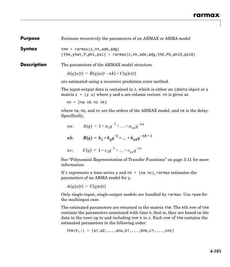
rarmax
4-161
4rarmaxPurpose Estimate recursively the parameters of an ARMAX or ARMA model
Syntax thm = rarmax(z,nn,adm,adg)[thm,yhat,P,phi,psi] = rarmax(z,nn,adm,adg,th0,P0,phi0,psi0)
Description The parameters of the ARMAX model structure
are estimated using a recursive prediction error method.
The input-output data is contained in z, which is either an iddata object or a matrix z = [y u] where y and u are column vectors. nn is given as
nn = [na nb nc nk]
where na, nb, and nc are the orders of the ARMAX model, and nk is the delay. Specifically,
See “Polynomial Representation of Transfer Functions” on page 3-11 for more information.
If z represents a time series y and nn = [na nc], rarmax estimates the parameters of an ARMA model for y.
Only single-input, single-output models are handled by rarmax. Use rpem for the multiinput case.
The estimated parameters are returned in the matrix thm. The kth row of thm contains the parameters associated with time k; that is, they are based on the data in the rows up to and including row k in z. Each row of thm contains the estimated parameters in the following order:
thm(k,:) = [a1,a2,...,ana,b1,...,bnb,c1,...,cnc]
A q( )y t( ) B q( )u t nk–( ) C q( )e t( )+=
na: A q( ) 1 a1q 1– … anaq na–+ + +=
nb: B q( ) b1 b+ 2q 1– … bnbq nb– 1++ +=nb: B q( ) b1 b+ 2q 1– … bnbq nb– 1++ +=
nc: C q( ) 1 c1q 1– … cncq nc–+ + +=
A q( )y t( ) C q( )e t( )=
rarmax
4-162
yhat is the predicted value of the output, according to the current model; that is, row k of yhat contains the predicted value of y(k) based on all past data.
The actual algorithm is selected with the two arguments adm and adg. These are described under rarx.
The input argument th0 contains the initial value of the parameters, a row vector consistent with the rows of thm. The default value of th0 is all zeros.
The arguments P0 and P are the initial and final values, respectively, of the scaled covariance matrix of the parameters. See rarx. The default value of P0 is 104 times the unit matrix. The arguments phi0, psi0, phi, and psi contain initial and final values of the data vector and the gradient vector, respectively. The sizes of these depend on the chosen model orders. The normal choice of phi0 and psi0 is to use the outputs from a previous call to rarmax with the same model orders. (This call could be a dummy call with default input arguments.) The default values of phi0 and psi0 are all zeros.
Note that the function requires that the delay nk be larger than 0. If you want nk = 0, shift the input sequence appropriately and use nk = 1.
Algorithm The general recursive prediction error algorithm (11.44), (11.47) through (11.49) of Ljung (1999) is implemented. See “Recursive Parameter Estimation” on page 3-85 for more information.
Examples Compute and plot, as functions of time, the four parameters in a second-order ARMA model of a time series given in the vector y. The forgetting factor algorithm with a forgetting factor of 0.98 is applied.
thm = rarmax(y,[2 2],'ff',0.98);plot(thm)
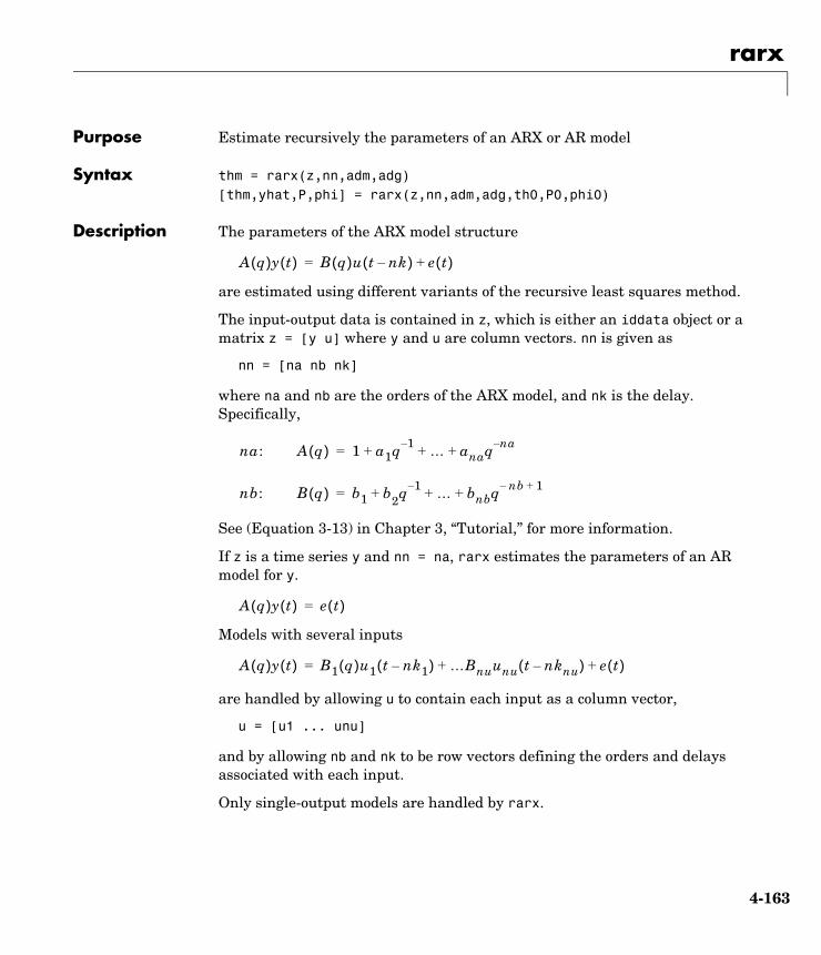
rarx
4-163
4rarxPurpose Estimate recursively the parameters of an ARX or AR model
Syntax thm = rarx(z,nn,adm,adg)[thm,yhat,P,phi] = rarx(z,nn,adm,adg,th0,P0,phi0)
Description The parameters of the ARX model structure
are estimated using different variants of the recursive least squares method.
The input-output data is contained in z, which is either an iddata object or a matrix z = [y u] where y and u are column vectors. nn is given as
nn = [na nb nk]
where na and nb are the orders of the ARX model, and nk is the delay. Specifically,
See (Equation 3-13) in Chapter 3, “Tutorial,” for more information.
If z is a time series y and nn = na, rarx estimates the parameters of an AR model for y.
Models with several inputs
are handled by allowing u to contain each input as a column vector,
u = [u1 ... unu]
and by allowing nb and nk to be row vectors defining the orders and delays associated with each input.
Only single-output models are handled by rarx.
A q( )y t( ) B q( )u t nk–( ) e t( )+=
na: A q( ) 1 a1q 1– … anaq na–+ + +=
nb: B q( ) b1 b+ 2q 1– … bnbq nb– 1++ +=
A q( )y t( ) e t( )=
A q( )y t( ) B1 q( )u1 t nk1–( ) …Bnuunu t nknu–( ) e t( )+ +=
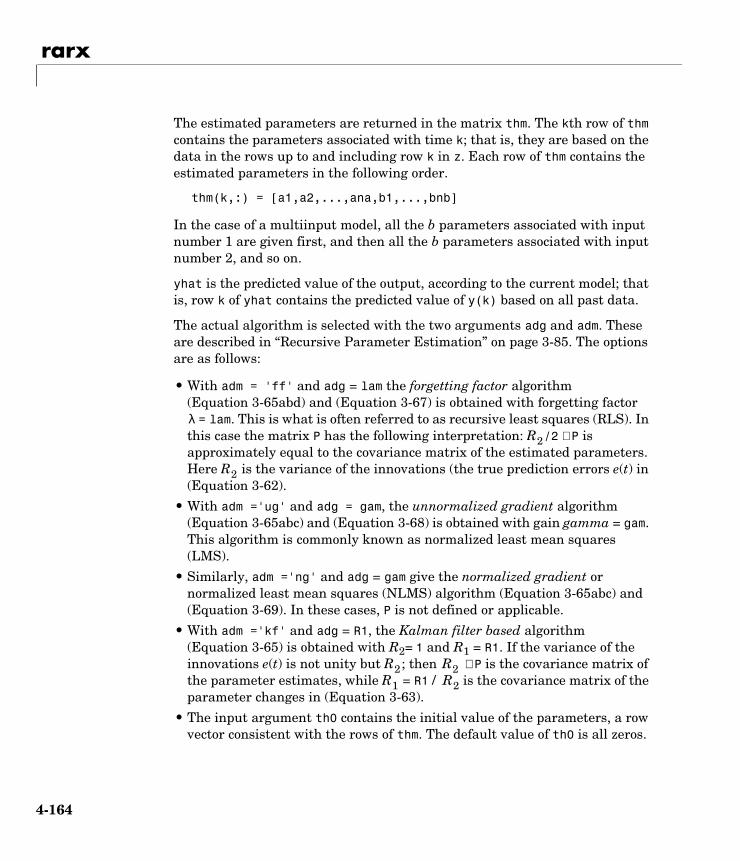
rarx
4-164
The estimated parameters are returned in the matrix thm. The kth row of thm contains the parameters associated with time k; that is, they are based on the data in the rows up to and including row k in z. Each row of thm contains the estimated parameters in the following order.
thm(k,:) = [a1,a2,...,ana,b1,...,bnb]
In the case of a multiinput model, all the b parameters associated with input number 1 are given first, and then all the b parameters associated with input number 2, and so on.
yhat is the predicted value of the output, according to the current model; that is, row k of yhat contains the predicted value of y(k) based on all past data.
The actual algorithm is selected with the two arguments adg and adm. These are described in “Recursive Parameter Estimation” on page 3-85. The options are as follows:
• With adm = 'ff' and adg = lam the forgetting factor algorithm (Equation 3-65abd) and (Equation 3-67) is obtained with forgetting factor = lam. This is what is often referred to as recursive least squares (RLS). In
this case the matrix P has the following interpretation: /2 ∗ P is approximately equal to the covariance matrix of the estimated parameters. Here is the variance of the innovations (the true prediction errors e(t) in (Equation 3-62).
• With adm ='ug' and adg = gam, the unnormalized gradient algorithm (Equation 3-65abc) and (Equation 3-68) is obtained with gain gamma = gam. This algorithm is commonly known as normalized least mean squares (LMS).
• Similarly, adm ='ng' and adg = gam give the normalized gradient or normalized least mean squares (NLMS) algorithm (Equation 3-65abc) and (Equation 3-69). In these cases, P is not defined or applicable.
• With adm ='kf' and adg = R1, the Kalman filter based algorithm (Equation 3-65) is obtained with R2= 1 and R1 = R1. If the variance of the innovations e(t) is not unity but ; then ∗ P is the covariance matrix of the parameter estimates, while = R1 / is the covariance matrix of the parameter changes in (Equation 3-63).
• The input argument th0 contains the initial value of the parameters, a row vector consistent with the rows of thm. The default value of th0 is all zeros.
λR2
R2
R2 R2R1 R2
rarx
4-165
• The arguments P0 and P are the initial and final values, respectively, of the scaled covariance matrix of the parameters. The default value of P0 is 104 times the identity matrix.
• The arguments phi0 and phi contain initial and final values, respectively, of the data vector.
Then, if
z = [y(1),u(1); ... ;y(N),u(N)]
you have phi0 = and phi = . The default value of phi0 is all zeros. For online use of rarx, use phi0, th0, and P0 as the previous outputs phi, thm (last row), and P.
Note that the function requires that the delay nk be larger than 0. If you want nk = 0, shift the input sequence appropriately and use nk = 1. See nkshift.
Examples Adaptive noise canceling: The signal y contains a component that has its origin in a known signal r. Remove this component by estimating, recursively, the system that relates r to y using a sixth-order FIR model together with the NLMS algorithm.
z = [y r];[thm,noise] = rarx(z,[0 6 1],'ng',0.1);% noise is the adaptive estimate of the noise% component of yplot(y-noise)
If the above application is a true online one, so that you want to plot the best estimate of the signal y - noise at the same time as the data y and u become available, proceed as follows.
phi = zeros(6,1); P=1000∗ eye(6);th = zeros(1,6); axis([0 100 -2 2]);plot(0,0,'∗ '), hold on% The loop:while ~abort[y,r,abort] = readAD(time);[th,ns,P,phi] = rarx([y r],'ff',0.98,th,P,phi);plot(time,y-ns,'∗ ')
ϕ t( ) y t 1–( ) … y t na–( ) u t 1–( ) …u t nb– nk– 1+( ), , , ,[ ]=
ϕ 1( ) ϕ N( )

rarx
4-166
time = time +Dtend
This example uses a forgetting factor algorithm with a forgetting factor of 0.98. readAD represents an M-file that reads the value of an A/D converter at the indicated time instant.
rbj
4-167
4rbjPurpose Estimate recursively the parameters of a Box-Jenkins model
Syntax thm = rbj(z,nn,adm,adg)[thm,yhat,P,phi,psi] = ... rbj(z,nn,adm,adg,th0,P0,phi0,psi0)
Description The parameters of the Box-Jenkins model structure
are estimated using a recursive prediction error method.
The input-output data is contained in z, which is either an iddata object or a matrix z = [y u] where y and u are column vectors. nn is given as
nn = [nb nc nd nf nk]
where nb, nc, nd, and nf are the orders of the Box-Jenkins model, and nk is the delay. Specifically,
See “Polynomial Representation of Transfer Functions” on page 3-11 for more information.
Only single-input, single-output models are handled by rbj. Use rpem for the multiinput case.
The estimated parameters are returned in the matrix thm. The kth row of thm contains the parameters associated with time k; that is, they are based on the data in the rows up to and including row k in z. Each row of thm contains the estimated parameters in the following order.
thm(k,:) = [b1,...,bnb,c1,...,cnc,d1,...,dnd,f1,...,fnf]
y t( ) B q( )F q( )------------u t nk–( ) C q( )
D q( )-------------e t( )+=
nb: B q( ) b1 b+ 2q 1– … bnbq nb– 1++ +=
nc: C q( ) 1 c1q 1– … cncq nc–+ + +=
nd: D q( ) 1 d1q 1– … dndq nd–+ + +=
nf: F q( ) 1 f1q 1– … fnfqnf–+ + +=
rbj
4-168
yhat is the predicted value of the output, according to the current model; that is, row k of yhat contains the predicted value of y(k) based on all past data.
The actual algorithm is selected with the two arguments adm and adg. These are described under rarx.
The input argument th0 contains the initial value of the parameters, a row vector consistent with the rows of thm. The default value of th0 is all zeros.
The arguments P0 and P are the initial and final values, respectively, of the scaled covariance matrix of the parameters. See rarx. The default value of P0 is 104 times the unit matrix. The arguments phi0, psi0, phi, and psi contain initial and final values of the data vector and the gradient vector, respectively. The sizes of these depend on the chosen model orders. The normal choice of phi0 and psi0 is to use the outputs from a previous call to rbj with the same model orders. (This call could be a dummy call with default input arguments.) The default values of phi0 and psi0 are all zeros.
Note that the function requires that the delay nk be larger than 0. If you want nk = 0, shift the input sequence appropriately and use nk = 1.
Algorithm The general recursive prediction error algorithm (11.44) of Ljung (1900) is implemented. See also “Recursive Parameter Estimation” on page 3-85.
realdata
4-169
4realdataPurpose Test if an iddata set is based on real-valued signals
Syntax realdata(data)
Description realdata returns 1 if
• data contains only real-valued signals.
• data contains frequency-domain signals, obtained by Fourier transformation of real-valued signals.
Otherwise realdata returns 0.
Notice the difference with isreal:
load iddata1isreal(z1); % returns 1zf = fft(z1);isreal(zf) % returns 0realdata(zf) % returns 1zf = complex(zf) % adds negative frequencies to zfrealdata(zf) % still returns 1
resample
4-170
4resamplePurpose Resample data by interpolation and decimation
Syntax datar = resample(data,P,Q)datar = resample(data,P,Q,,filter_order)
Description data: The data to be resampled, given as an iddata object
datar: The resampled data returned as an iddata object
P, Q: Integers that determine the resampling factor. The new sampling interval will be Q/P times the original one, so resample(z,1,Q) means decimation with a factor Q.
filter_order: Determines the order of the presampling filters used before interpolation and decimation. Default is 10.
Algorithm If the Signal Processing Toolbox is available, the resampling is achieved by calls to the resample function in that toolbox. The intersample character of the input, as described by data.InterSample, is taken into account.
Otherwise, the data is interpolated by a factor P and then decimated by a factor Q. The interpolation and decimation are preceded by prefiltering, and follow the same algorithms as in the routines interp and decimate in the Signal Processing Toolbox.
Examples Resample by increasing the sampling rate by a factor of 1.5 and compare the signals.
plot(u)ur = resample(u,3,2);plot(u,ur)
resid
4-171
4residPurpose Compute and test the residuals (prediction errors) of a model
Syntax resid(m,data)resid(m,data,Type)resid(m,data,Type,M)e = resid(m,data);
Description data contains the output-input data as an iddata object. Both time-domain and frequency-domain data are supported. data can also be an idfrd object.
m is the model to be evaluated on the given data set. It is any idmodel object.
In all cases the residuals e associated with the data and the model are computed. This is done as in the command pe with a default choice of init.
When called without output arguments, resid produces a plot. The plot can be of three kinds depending on the argument Type:
• Type = 'Corr' (only available for time-domain data): The autocorrelation function of e and the cross correlation between e and the input(s) u are computed and displayed. The 99% confidence intervals for these values are also computed and shown as a yellow region. The computation of the confidence region is done assuming e to be white and independent of u. The functions are displayed up to lag M, which is 25 by default.
• Type = 'ir': The impulse response (up to lag M, which is 25 by default) from the input to the residuals is plotted with a 99% confidence region around zero marked as a yellow area. Negative lags up to M/4 are also included to investigate feedback effects. (The result is the same as impulse(e,'sd',2.58,'fill',M).)
• Type = 'fr': The frequency response from the input to the residuals (based on a high-order FIR model) is shown as a Bode plot. A 99% confidence region around zero is also marked as a yellow area.
The default for time-domain data is Type = 'Corr'. For frequency-domain data, the default is Type = 'fr'.
With an output argument, no plot is produced, and e is returned with the residuals (prediction errors) associated with the model and the data. It is an iddata object with the residuals as outputs and the input in data as inputs. That means that e can be directly used to build model error models, that is,
resid
4-172
models that describe the dynamics from the input to the residuals (which should be negligible if m is a good description of the system).
See “Model Structure Selection and Validation” on page 3-70 for more information.
Examples Here are some typical model validation commands.
e = resid(m,data);plot(e)compare(data,m);
To compute a model error model, that is, a model to input to the residuals to see if any essential unmodeled dynamics are left, do the following:
e = resid(m,data);me = arx(e,[10 10 0]);bode(me,'sd',3,fill')
See Also compare, idgrey, idarx, idpoly, idproc, idss, pem
References Ljung (1999), Section 16.6.
roe
4-173
4roePurpose Estimate recursively the parameters of an output-error model
Syntax thm = roe(z,nn,adm,adg)[thm,yhat,P,phi,psi] = roe(z,nn,adm,adg,th0,P0,phi0,psi0)
Description The parameters of the output-error model structure
are estimated using a recursive prediction error method.
The input-output data are contained in z, which is either an iddata object or a matrix z = [y u] where y and u are column vectors. nn is given as
nn = [nb nf nk]
where nb and nf are the orders of the output-error model, and nk is the delay. Specifically,
See “Polynomial Representation of Transfer Functions” on page 3-11 for more information.
Only single-input, single-output models are handled by roe. Use rpem for the multiinput case.
The estimated parameters are returned in the matrix thm. The kth row of thm contains the parameters associated with time k; that is, they are based on the data in the rows up to and including row k in z.
Each row of thm contains the estimated parameters in the following order.
thm(k,:) = [b1,...,bnb,f1,...,fnf]
yhat is the predicted value of the output, according to the current model; that is, row k of yhat contains the predicted value of y(k) based on all past data.
The actual algorithm is selected with the two arguments adg and adm. These are described under rarx.
y t( ) B q( )F q( )------------u t nk–( ) e t( )+=
nb: B q( ) b1 b+ 2q 1– … bnbq nb– 1++ +=
nf: F q( ) 1 f1q 1– … fnfqnf–+ + +=
roe
4-174
The input argument th0 contains the initial value of the parameters, a row vector consistent with the rows of thm. The default value of th0 is all zeros.
The arguments P0 and P are the initial and final values, respectively, of the scaled covariance matrix of the parameters. See rarx. The default value of P0 is 104 times the unit matrix. The arguments phi0, psi0, phi, and psi contain initial and final values of the data vector and the gradient vector, respectively. The sizes of these depend on the chosen model orders. The normal choice of phi0 and psi0 is to use the outputs from a previous call to roe with the same model orders. (This call could be a dummy call with default input arguments.) The default values of phi0 and psi0 are all zeros.
Note that the function requires that the delay nk be larger than 0. If you want nk = 0, shift the input sequence appropriately and use nk = 1.
Algorithm The general recursive prediction error algorithm (11.44) of Ljung (1999) is implemented. See also “Recursive Parameter Estimation” on page 3-85.
See Also oe, rarx, rbj, rplr, rpem, nkshift
rpem
4-175
4rpemPurpose Estimate recursively the parameters of a general multiinput single-output linear model
Syntax thm = rpem(z,nn,adm,adg)[thm,yhat,P,phi,psi] = rpem(z,nn,adm,adg,th0,P0,phi0,psi0)
Description The parameters of the general linear model structure
are estimated using a recursive prediction error method.
The input-output data is contained in z, which is either an iddata object or a matrix z = [y u] where y and u are column vectors. (In the multiinput case, u contains one column for each input.) nn is given as
nn = [na nb nc nd nf nk]
where na, nb, nc, nd, and nf are the orders of the model, and nk is the delay. For multiinput systems, nb, nf, and nk are row vectors giving the orders and delays of each input. See “Polynomial Representation of Transfer Functions” on page 3-11 for an exact definition of the orders.
The estimated parameters are returned in the matrix thm. The kth row of thm contains the parameters associated with time k; that is, they are based on the data in the rows up to and including row k in z. Each row of thm contains the estimated parameters in the following order.
thm(k,:) = [a1,a2,...,ana,b1,...,bnb,... c1,...,cnc,d1,...,dnd,f1,...,fnf]
For multiinput systems, the B part in the above expression is repeated for each input before the C part begins, and the F part is also repeated for each input. This is the same ordering as in m.par.
yhat is the predicted value of the output, according to the current model; that is, row k of yhat contains the predicted value of y(k) based on all past data.
The actual algorithm is selected with the two arguments adg and adm. These are described under rarx.
A q( )y t( )B1 q( )F1 q( )---------------u1 t nk1–( ) …
Bnu q( )Fnu q( )------------------- unu t nknu–( ) C q( )
D q( )-------------e t( )+ + +=
rpem
4-176
The input argument th0 contains the initial value of the parameters, a row vector consistent with the rows of thm. The default value of th0 is all zeros.
The arguments P0 and P are the initial and final values, respectively, of the scaled covariance matrix of the parameters. See rarx. The default value of P0 is 104 times the unit matrix. The arguments phi0, psi0, phi, and psi contain initial and final values of the data vector and the gradient vector, respectively. The sizes of these depend on the chosen model orders. The normal choice of phi0 and psi0 is to use the outputs from a previous call to rpem with the same model orders. (This call could be a dummy call with default input arguments.) The default values of phi0 and psi0 are all zeros.
Note that the function requires that the delay nk be larger than 0. If you want nk = 0, shift the input sequence appropriately and use nk = 1.
Algorithm The general recursive prediction error algorithm (11.44) of Ljung (1999) is implemented. See also “Recursive Parameter Estimation” on page 3-85.
For the special cases of ARX/AR models, and of single-input ARMAX/ARMA, Box-Jenkins, and output-error models, it is more efficient to use rarx, rarmax, rbj, and roe.
See Also pem, rarmax, rarx, rbj, roe, rplr, nkshift
rplr
4-177
4rplrPurpose Estimate recursively the parameters of a general multiinput single-output linear model
Syntax thm = rplr(z,nn,adm,adg)[thm,yhat,P,phi] = rplr(z,nn,adm,adg,th0,P0,phi0)
Description This is a direct alternative to rpem and has essentially the same syntax. See rpem for an explanation of the input and output arguments.
rplr differs from rpem in that it uses another gradient approximation. See Section 11.5 in Ljung (1999). Several of the special cases are well-known algorithms.
When applied to ARMAX models, (nn = [na nb nc 0 0 nk]), rplr gives the extended least squares (ELS) method. When applied to the output-error structure (nn = [0 nb 0 0 nf nk]), the method is known as HARF in the adm = 'ff' case and SHARF in the adm = 'ng' case.
rplr can also be applied to the time-series case in which an ARMA model is estimated with
z = ynn = [na nc]
You can thus use rplr as an alternative to rarmax for this case.
See Also pem, rarmax, rarx, rbj, roe, rpem
segment
4-178
4segmentPurpose Segment data and estimate models for each segment
Syntax segm = segment(z,nn) [segm,V,thm,R2e] = segment(z,nn,R2,q,R1,M,th0,P0,ll,mu)
Description segment builds models of AR, ARX, or ARMAX/ARMA type,
assuming that the model parameters are piecewise constant over time. It results in a model that has split the data record into segments over which the model remains constant. The function models signals and systems that might undergo abrupt changes.
The input-output data is contained in z, which is either an iddata object or a matrix z = [y u] where y and u are column vectors. If the system has several inputs, u has the corresponding number of columns.
The argument nn defines the model order. For the ARMAX model
nn = [na nb nc nk]
where na, nb, and nc are the orders of the corresponding polynomials. See “Polynomial Representation of Transfer Functions” on page 3-11. Moreover, nk is the delay. If the model has several inputs, nb and nk are row vectors, giving the orders and delays for each input.
For an ARX model (nc = 0) enter
nn = [na nb nk]
For an ARMA model of a time series
z = ynn = [na nc]
and for an AR model
nn = na
The output argument segm is a matrix, whose k row contains the parameters corresponding to time k. This is analogous to the output argument thm in rarx and rarmax. The output argument thm of segment contains the corresponding model parameters that have not yet been segmented. That is, they are not
A q( )y t( ) B q( )u t nk–( ) C q( )e t( )+=
segment
4-179
piecewise constant, and therefore correspond to the outputs of the functions rarmax and rarx. In fact, segment is an alternative to these two algorithms, and has a better capability to deal with time variations that might be abrupt.
The output argument V contains the sum of the squared prediction errors of the segmented model. It is a measure of how successful the segmentation has been.
The input argument R2 is the assumed variance of the innovations e(t) in the model. The default value of R2, R2 = [], is that it is estimated. Then the output argument R2e is a vector whose kth element contains the estimate of R2 at time k.
The argument q is the probability that the model undergoes at an abrupt change at any given time. The default value is 0.01.
R1 is the assumed covariance matrix of the parameter jumps when they occur. The default value is the identity matrix with dimension equal to the number of estimated parameters.
M is the number of parallel models used in the algorithm (see below). Its default value is 5.
th0 is the initial value of the parameters. Its default is zero. P0 is the initial covariance matrix of the parameters. The default is 10 times the identity matrix.
ll is the guaranteed life of each of the models. That is, any created candidate model is not abolished until after at least ll time steps. The default is ll = 1. Mu is a forgetting parameter that is used in the scheme that estimates R2. The default is 0.97.
The most critical parameter for you to choose is R2. It is usually more robust to have a reasonable guess of R2 than to estimate it. Typically, you need to try different values of R2 and evaluate the results. (See the example below.) sqrt(R2) corresponds to a change in the value y(t) that is normal, giving no indication that the system or the input might have changed.
segment
4-180
Algorithm The algorithm is based on M parallel models, each recursively estimated by an algorithm of Kalman filter type. Each is updated independently, and its posterior probability is computed. The time-varying estimate thm is formed by weighting together the M different models with weights equal to their posterior probability. At each time step the model (among those that have lived at least 11 samples) that has the lowest posterior probability is abolished. A new model is started, assuming that the system parameters have jumped, with probability q, a random jump from the most likely among the models. The covariance matrix of the parameter change is set to R1.
After all the data are examined, the surviving model with the highest posterior probability is tracked back and the time instances where it jumped are marked. This defines the different segments of the data. (If no models had been abolished in the algorithm, this would have been the maximum likelihood estimates of the jump instances.) The segmented model segm is then formed by smoothing the parameter estimate, assuming that the jump instances are correct. In other words, the last estimate over a segment is chosen to represent the whole segment.
Examples Check how the algorithm segments a sinusoid into segments of constant levels. Then use a very simple model y(t) = b1 * 1, where 1 is a fake input and describes the piecewise constant level of the signal y(t) (which is simulated as a sinusoid).
y = sin([1:50]/3)';thm = segment([y,ones(y)],[0 1 1],0.1);plot([thm,y])
By trying various values of R2 (0.1 in the above example), more levels are created as R2 decreases.
b1
selstruc
4-181
4selstrucPurpose Select model order (structure)
Syntax nn = selstruc(v)[nn,vmod] = selstruc(v,c)
Description selstruc is a function to help choose a model structure (order) from the information contained in the matrix v obtained as the output from arxstruc or ivstruc.
The default value of c is 'plot'. The plot shows the percentage of the output variance that is not explained by the model as a function of the number of parameters used. Each value shows the best fit for that number of parameters. By clicking in the plot you can examine which orders are of interest. When you click 'Select', the variable nn is returned in the workspace as the optimal model structure for your choice of number of parameters. Several choices can be made.
c = 'aic' gives no plots, but returns in nn the structure that minimizes Akaike’s Information Criterion (AIC),
where V is the loss function, d is the total number of parameters in the structure in question, and N is the number of data points used for the estimation. See aic for more details.
c = 'mdl' returns in nn the structure that minimizes Rissanen’s Minimum Description Length (MDL) criterion.
When c equals a numerical value, the structure that minimizes
is selected.
Vmod V 1 2dN-------+
=
Vmod V 1 d N( )logN
----------------------+ =
Vmod V 1 cdN------+
=
selstruc
4-182
The output argument vmod has the same format as v, but it contains the logarithms of the accordingly modified criteria.
Examples V = arxstruc(data(1:200),data(201:400),struc(1:10,1:10,1:10))nn = selstruc(V,0); %best fit to validation datam = arx(data,nn)
set
4-183
4setPurpose Set or modify the properties of models and iddata sets
Syntax set(m,'Property',Value)set(m,'Property1',Value1,...'PropertyN',ValueN)set(m,'Property')set(m)
Description set is used to set or modify the properties of any of the objects in the toolbox (iddata, idmodel, idgrey, idarx, idpoly, idss). See the corresponding reference pages for a complete list of properties.
set(m,'Property',Value) assigns the value Value to the property of the object m specified by the string 'Property'. This string can be the full property name (for example, 'SSParameterization') or any unambiguous case-insensitive abbreviation (for example, 'ss').
set(m,'Property1',Value1,...'PropertyN',ValueN) sets multiple properties with a single statement. In certain cases this might be necessary, since the model m must, for example, have state-space matrices of consistent dimensions after each set statement.
set(m,'Property') displays admissible values for the property specified by 'Property'.
set(m) displays all assignable values of m and their admissible values.
The same result is also obtained by subassignment.
m.Property = Value
setstruc
4-184
4setstrucPurpose Set the structure matrices for idss objects in an efficient manner
Syntax setstruc(M,As,Bs,Cs,Ds.Ks,X0s)setstruc(M,Mods)
Description setstruc(M,As,Bs,Cs,Ds.Ks,X0s)
is the same as
set(M,'As',As,'Bs',Bs,'Cs',Cs,'Ds',Ds,'Ks',Ks,'X0s',X0s)
Use empty matrices for structure matrices that should not be changed. You can omit trailing arguments.
In the alternative syntax, Mods is a structure with fieldnames As, Bs, etc., with the corresponding values of the fields.
See Also idss
setpname
4-185
4setpnamePurpose Assign mnemonic parameter names to black-box model structures
Syntax model = setpname(model)
Description model is an idmodel object of idarx, idpoly, idproc, or idss type. The returned model has the 'PName' property set to a cell array of strings that correspond to the symbols used in this manual to describe the parameters.
For single-input idpoly models, the parameters are called 'a1', 'a2', ...,'fn', as defined in “Polynomial Representation of Transfer Functions” on page 3-11.
For multiinput idpoly models, the b and f parameters have the output/input channel number in parentheses, as in 'b1(1,2)', 'f3(1,2)', etc.
For idarx models, the parameter names are as in '-A(ky,ku)' for the negative value of the ky-ku entry of the matrix in (Equation 3-50) and similarly for the B parameters.
For idss models, the parameters are named for the matrix entries they represent, such as 'A(4,5)', 'K(2,3)', etc.
For idproc models, the parameter names are as described under idproc.
This function is particularly useful when certain parameters are to be fixed. See the property FixedParameter under Algorithm Properties.
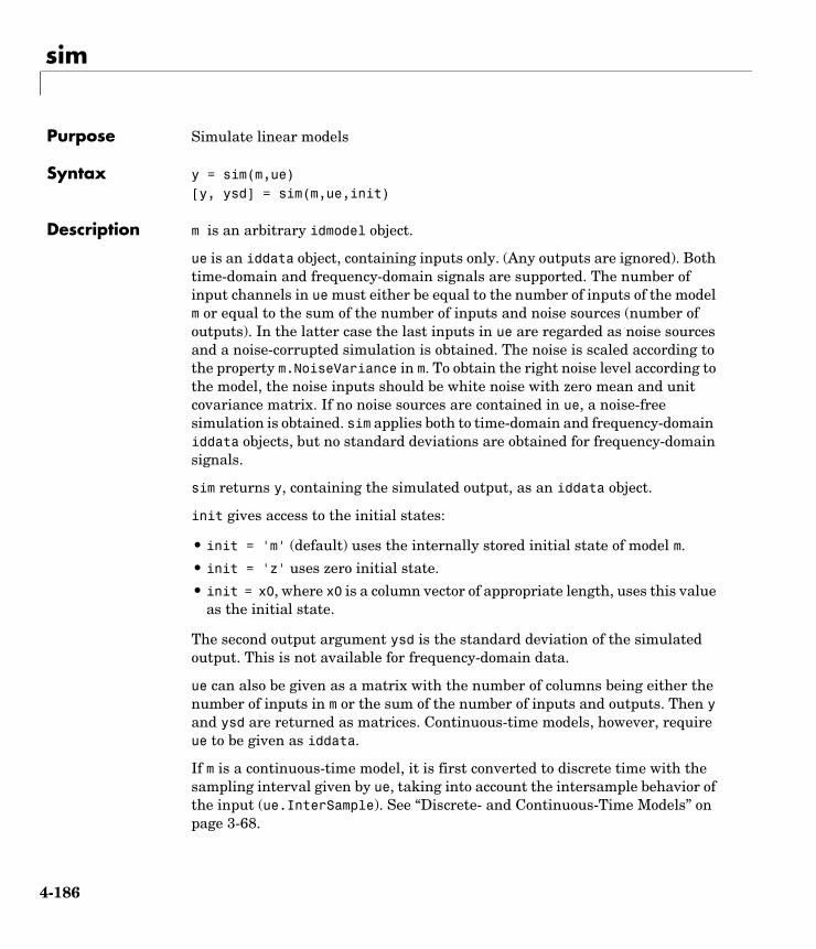
sim
4-186
4simPurpose Simulate linear models
Syntax y = sim(m,ue)[y, ysd] = sim(m,ue,init)
Description m is an arbitrary idmodel object.
ue is an iddata object, containing inputs only. (Any outputs are ignored). Both time-domain and frequency-domain signals are supported. The number of input channels in ue must either be equal to the number of inputs of the model m or equal to the sum of the number of inputs and noise sources (number of outputs). In the latter case the last inputs in ue are regarded as noise sources and a noise-corrupted simulation is obtained. The noise is scaled according to the property m.NoiseVariance in m. To obtain the right noise level according to the model, the noise inputs should be white noise with zero mean and unit covariance matrix. If no noise sources are contained in ue, a noise-free simulation is obtained. sim applies both to time-domain and frequency-domain iddata objects, but no standard deviations are obtained for frequency-domain signals.
sim returns y, containing the simulated output, as an iddata object.
init gives access to the initial states:
• init = 'm' (default) uses the internally stored initial state of model m.
• init = 'z' uses zero initial state.
• init = x0, where x0 is a column vector of appropriate length, uses this value as the initial state.
The second output argument ysd is the standard deviation of the simulated output. This is not available for frequency-domain data.
ue can also be given as a matrix with the number of columns being either the number of inputs in m or the sum of the number of inputs and outputs. Then y and ysd are returned as matrices. Continuous-time models, however, require ue to be given as iddata.
If m is a continuous-time model, it is first converted to discrete time with the sampling interval given by ue, taking into account the intersample behavior of the input (ue.InterSample). See “Discrete- and Continuous-Time Models” on page 3-68.
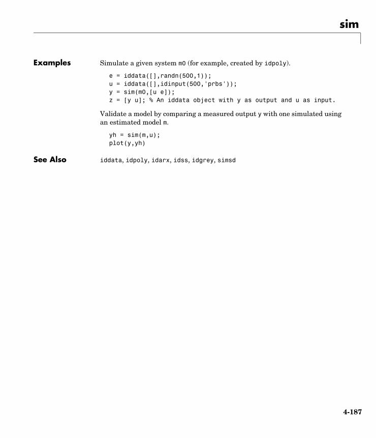
sim
4-187
Examples Simulate a given system m0 (for example, created by idpoly).
e = iddata([],randn(500,1));u = iddata([],idinput(500,'prbs'));y = sim(m0,[u e]);z = [y u]; % An iddata object with y as output and u as input.
Validate a model by comparing a measured output y with one simulated using an estimated model m.
yh = sim(m,u);plot(y,yh)
See Also iddata, idpoly, idarx, idss, idgrey, simsd
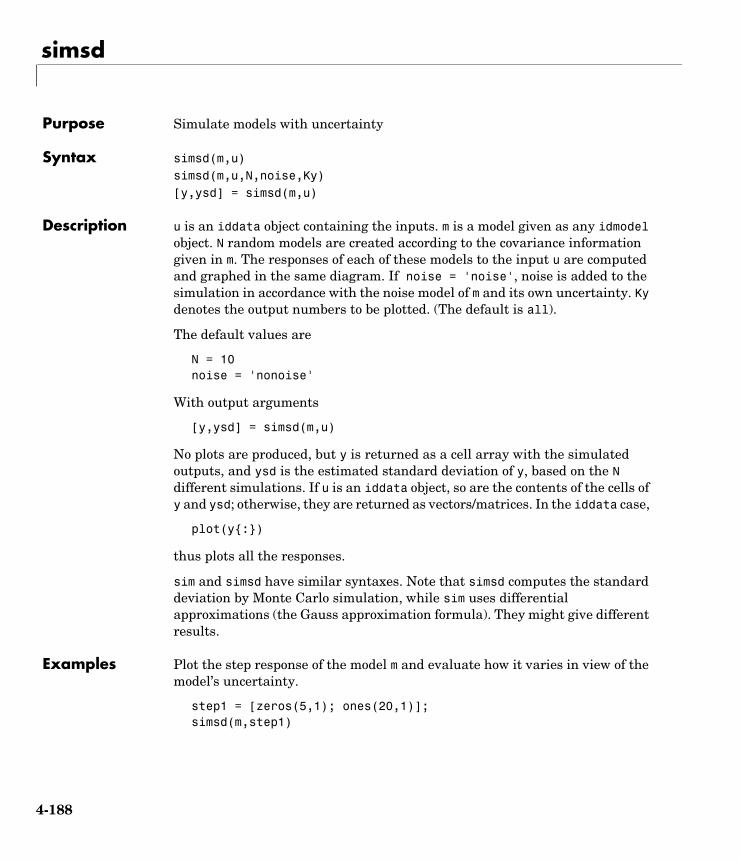
simsd
4-188
4simsdPurpose Simulate models with uncertainty
Syntax simsd(m,u)simsd(m,u,N,noise,Ky)[y,ysd] = simsd(m,u)
Description u is an iddata object containing the inputs. m is a model given as any idmodel object. N random models are created according to the covariance information given in m. The responses of each of these models to the input u are computed and graphed in the same diagram. If noise = 'noise', noise is added to the simulation in accordance with the noise model of m and its own uncertainty. Ky denotes the output numbers to be plotted. (The default is all).
The default values are
N = 10noise = 'nonoise'
With output arguments
[y,ysd] = simsd(m,u)
No plots are produced, but y is returned as a cell array with the simulated outputs, and ysd is the estimated standard deviation of y, based on the N different simulations. If u is an iddata object, so are the contents of the cells of y and ysd; otherwise, they are returned as vectors/matrices. In the iddata case,
plot(y{:})
thus plots all the responses.
sim and simsd have similar syntaxes. Note that simsd computes the standard deviation by Monte Carlo simulation, while sim uses differential approximations (the Gauss approximation formula). They might give different results.
Examples Plot the step response of the model m and evaluate how it varies in view of the model’s uncertainty.
step1 = [zeros(5,1); ones(20,1)];simsd(m,step1)

simsd
4-189
See Also sim
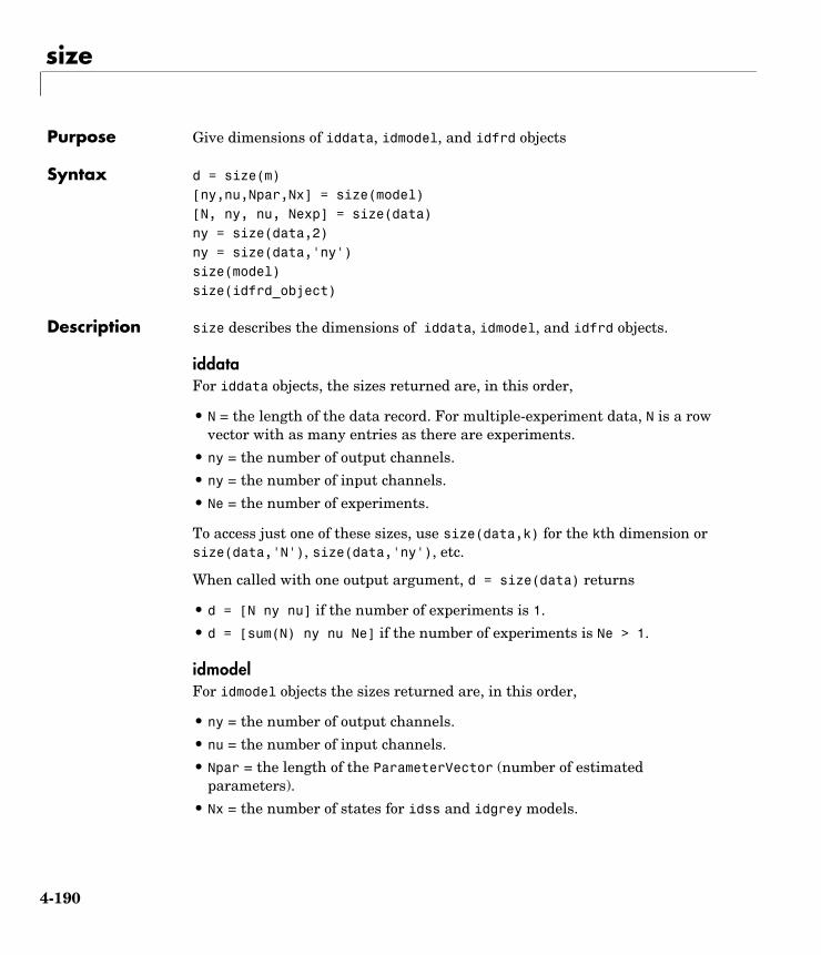
size
4-190
4sizePurpose Give dimensions of iddata, idmodel, and idfrd objects
Syntax d = size(m)[ny,nu,Npar,Nx] = size(model)[N, ny, nu, Nexp] = size(data)ny = size(data,2)ny = size(data,'ny')size(model)size(idfrd_object)
Description size describes the dimensions of iddata, idmodel, and idfrd objects.
iddataFor iddata objects, the sizes returned are, in this order,
• N = the length of the data record. For multiple-experiment data, N is a row vector with as many entries as there are experiments.
• ny = the number of output channels.
• ny = the number of input channels.
• Ne = the number of experiments.
To access just one of these sizes, use size(data,k) for the kth dimension or size(data,'N'), size(data,'ny'), etc.
When called with one output argument, d = size(data) returns
• d = [N ny nu] if the number of experiments is 1.
• d = [sum(N) ny nu Ne] if the number of experiments is Ne > 1.
idmodelFor idmodel objects the sizes returned are, in this order,
• ny = the number of output channels.
• nu = the number of input channels.
• Npar = the length of the ParameterVector (number of estimated parameters).
• Nx = the number of states for idss and idgrey models.

size
4-191
In this case the individual dimensions are obtained by size(mod,2), size(mod,'Npar'), etc.
When size is called with one output argument, d = size(mod), d is given by
[ny nu Npar]
idfrdFor idfrd models, the sizes returned are, in this order,
• ny = the number of output channels.
• nu = the number of input channels.
• Nf = the number of frequencies.
• Ns = the number of spectrum channels.
In this case the individual dimensions are obtained by size(mod,2), size(mod,'Nf'), etc.
When size is called with one output argument, d = size(fre), d is given by
[ny nu Nf Ns]
When size is called with no output arguments, in any of these cases, the information is displayed in the MATLAB Command Window.

spa
4-192
4spaPurpose Estimate frequency response and spectrum by spectral analysis
Syntax g = spa(data)g = spa(data,M,w,maxsize)[g,phi,spe] = spa(data)
Description spa estimates the transfer function g and the noise spectrum of the general linear model
where is the spectrum of .
data contains the output-input data as an iddata object. The data can be complex valued. data can be both time domain and frequency domain. data can also be an idfrd object.
g is returned as an idfrd object (see idfrd) with the estimate of at the frequencies specified by row vector w. The default value of w is
w = [1:128]/128∗ pi/Ts
Here Ts is the sampling interval of data.
g also includes information about the spectrum estimate of at the same frequencies. Both outputs are returned with estimated covariances, included in g. See idfrd.
M is the length of the lag window used in the calculations. The default value is
M = min(30,length(data)/10)
Changing the value of M controls the frequency resolution of the estimate. The resolution corresponding to M is approximately /M rad/sampling interval. The value of M exchanges bias for variance in the spectral estimate. As M is increased, the estimated functions show more detail, but are more corrupted by noise. The sharper peaks a true frequency function has, the higher M it needs. See etfe as an alternative for narrowband signals and systems. The function spafdr allows the frequency resolution to depend on the frequency. See also “Estimating Spectra and Frequency Functions” on page 3-15.
maxsize controls the memory-speed tradeoff (see Algorithm Properties).
Φv
y t( ) G q( )u t( ) v t( )+=
Φv ω( ) v t( )
G eiω( )ω
Φv ω( )
π
spa
4-193
For time series, where data contains no input channels, g is returned with the estimated output spectrum and its estimated standard deviation.
When spa is called with two or three output arguments,
• g is returned as an idfrd model with just the estimated frequency response from input to output and its uncertainty.
• phi is returned as an idfrd model, containing just the spectrum data for the output spectrum and its uncertainty.
• spe is returned as an idfrd model containing spectrum data for all output-input channels in data. That is, if z = [data.OutputData, data.InputData], spe contains as spectrum data the matrix-valued power spectrum of z.
Here win(m) is weight at lag m of an M-size Hamming window and W is the frequency value i rad/s. Note that ' denotes complex-conjugate transpose.
The normalization of the spectrum differs from the one used by spectrum in the Signal Processing Toolbox. See “Spectrum Normalization and the Sampling Interval” on page 3-103 for a more precise definition.
Examples With default frequencies,
g = spa(z);bode(g)
With logarithmically spaced frequencies,
w = logspace(-2,pi,128);g= spa(z,[],w); % (empty matrix gives default)bode(g,'sd',3)bode(g('noise'),'sd',3) % The noise spectrum with confidence interval of 3 standard deviations.
Φv ω( )
S Ez t m+( )z t( )′ iWmT–( )exp win m( )
m M–=
M
∑=
spa
4-194
Algorithm The covariance function estimates are computed using covf. These are multiplied by a Hamming window of lag size M and then transformed using a Fourier transform. The relevant ratios and differences are then formed. For the default frequencies, this is done using a fast Fourier transform, which is more efficient than for user-defined frequencies. For multivariable systems, a straightforward for loop is used.
Note that M = is in Table 6.1 of Ljung (1999). The standard deviations are computed as on pages 184 and 188 in Ljung (1999).
See Also bode, etfe, idfrd, nyquist, spafdr
γ
spafdr
4-195
4 spafdrPurpose Estimate frequency response and spectrum by spectral analysis with frequency dependent resolution
Syntax g = spafdr(data)g = spafdr(data,Resol,w)
Description spafdr estimates the transfer function g and the noise spectrum of the general linear model
where is the spectrum of .
data contains the output-input data as an iddata object. The data can be complex valued, and either time or frequency domain. It can also be an idfrd object containing frequency-response data.
g is returned as an idfrd object (see idfrd) with the estimate of at the frequencies specified by row vector w. g also includes information about the spectrum estimate of at the same frequencies. Both results are returned with estimated covariances, included in g. See idfrd. The normalization of the spectrum is the same as described under spa.
FrequenciesThe frequency variable w is either specified as a row vector of frequencies, or as a cell array {wmin,wmax}. In the latter case the covered frequencies will be 50 logarithmically spaced points from wmin to wmax. You can change the number of points to NP by entering {wmin,wmax,NP}.
Omitting w or entering it as an empty matrix gives the default value, which is 100 logarithmically spaced frequencies between the smallest and largest frequency in data. For time-domain data, this means from 1/N*Ts to pi*Ts, where Ts is the sampling interval of data and N is the number of data.
ResolutionThe argument Resol defines the frequency resolution of the estimates. The resolution (measured in rad/s) is the size of the smallest detail in the frequency function and the spectrum that is resolved by the estimate. The resolution is a tradeoff between obtaining estimates with fine, reliable details, and suffering from spurious, random effects: The finer the resolution, the higher the variance
Φv
y t( ) G q( )u t( ) v t( )+=
Φv ω( ) v t( )
G eiω( )ω
Φv ω( )
spafdr
4-196
in the estimate. Resol can be entered as a scalar (measured in rad/s), which defines the resolution over the whole frequency interval. It can also be entered as a row vector of the same length as w. Then Resol(k) is the local, frequency-dependent resolution around frequency w(k).
The default value of Resol, obtained by omitting it or entering it as the empty matrix, is Resol(k) = 2(w(k+1)-w(k)), adjusted upwards, so that a reasonable estimate is guaranteed. In all cases, the resolution is returned in the variable g.EstimationInfo.WindowSize.
Algorithm If the data is given in the time domain, it is first converted to the frequency domain. Then averages of Y(w)Conj(U(w)) and U(w)Conj(U(w)) are formed over the frequency ranges w, corresponding to the desired resolution around the frequency in question. The ratio of these averages is then formed for the frequency-function estimate, and corresponding expressions define the noise spectrum estimate.
See Also bode, etfe, idfrd, nyquist, spa
ss, tf, zpk, frd
4-197
4ss, tf, zpk, frdPurpose Transform the model objects of the System Identification Toolbox to the LTI models of the Control System Toolbox
Syntax sys = ss(mod)sys = ss(mod,'m')sys = tf(mod)sys = zpk(mod)sys = frd(mod)
Description mod is any idmodel object: idgrey, idarx, idpoly, idproc, idss, idmodel, or idfrd. However, idfrd objects can only be converted to frd objects.
sys is returned as the indicated LTI model. The noise input channels in mod are treated as follows:
Consider a model mod with both measured input channels u (nu channels) and noise channels e (ny channels) with covariance matrix
where L is a lower triangular matrix. Note that mod.NoiseVariance = . The model can also be described with a unit variance, normalized noise source v.
For ss, tf, and zpk, both measured input channels u and normalized noise input channels v in mod will be input channels in sys. The noise input channels will belong to the InputGroup 'Noise', while the others belong to the InputGroup 'Measured'. The names of the noise input channels will be v@yname, where yname is the name of the corresponding output channel. This means that the LTI object realizes the transfer function [G HL].
For frd, no noise information is included.
To transform only the measured input channels in sys, use
sys = ss(mod('m')) or sys = ss(mod,'m')
and analogously for tf and zpk. This will give a representation of just G.
Λ
y Gu He+=cov e( ) Λ LL ′= =
Λ
y Gu HLv+=cov v( ) I=

ss, tf, zpk, frd
4-198
For a time series, (no measured input channels, nu = 0), the LTI representations in ss, tf, zpk, and frd contain the transfer functions from the normalized noise sources v to the outputs, that is, HL. If the model m has both measured and noise inputs, sys = ss(mod('n')) gives a representation of the additive noise. For frd no output is given for a time-series model.
In addition, the normal subreferencing can be used.
sys = ss(mod(1,[3 4]))
If you want to describe [G H] or H (unnormalized noise), from e to y, first use
mod = noisecnv(mod)
to convert the noise channels e to regular input channels. These channels will have the names e@yname.

ssdata
4-199
4ssdataPurpose Transform a model to state-space form
Syntax [A,B,C,D,K,X0] = ssdata(m)[A,B,C,D,K,X0,dA,dB,dC,dD,dK,dX0] = ssdata(m)
Description m is the model given as any idmodel object. A, B, C, D, K, and X0 are the matrices in the state-space description
where is or depending on whether m is a continuous-time or discrete-time model.
dA, dB, dC, dD, dK, and dX0 are the standard deviations of the state-space matrices.
If the underlying model itself is a state-space model, the matrices correspond to the same basis. If the underlying model is an input-output model, an observer canonical form representation is obtained.
For a time-series model (no measured input channels, u = []), B and D are returned as the empty matrices.
Subreferencing models in the usual way (see idmodel properties) will give the state-space representation of the chosen channels. Notice in particular that
[A,B,C,D] = ssdata(m('m'))
gives the response from the measured inputs. This is a model without a disturbance description. Moreover,
[A,B,C,D,K] = ssdata(m('n'))
('n' as in “noise”) gives the disturbance description, that is, a time-series description of the additive noise with no measured inputs, so that B = [] and D = [].
x t( ) Ax t( ) Bu t( ) Ke t( )+ +=
x 0( ) x0=
y t( ) Cx t( ) Dx t( ) e t( )+ +=
x t( ) x· t( ) x t Ts+( )
ssdata
4-200
To obtain state-space descriptions that treat all input channels, both u and e, as measured inputs, first apply the conversion
m = noisecnv(m)
or
m = noisecnv(m,'norm')
where the latter case first normalizes e to v, where v has a unit covariance matrix. See the reference page for noisecnv.
Algorithm The computation of the standard deviations in the input-output case assumes that an A polynomial is not used together with an F or D polynomial in (Equation 3-43). For the computation of standard deviations in the case that the state-space parameters are complicated functions of the parameters, the Gauss approximation formula is used together with numerical derivatives. The step sizes for this differentiation are determined by nuderst.
See Also idmodel, idss, nuderst
step
4-201
4stepPurpose Estimate/compute/display step response
Syntax step(m)step(data)step(m,'sd',sd,Time)step(data,'sd',sd,'PW',na,Time)step(m1,m2,...,dat1, ...,mN,Time,'sd',sd)step(m1,'PlotStyle1',m2,'PlotStyle2',...,dat1,'PlotStylek',...,mN,
'PlotStyleN',Time,'sd',sd)[y,t,ysd] = step(m)mod = step(data)
Description step can be applied both to idmodels and to iddata sets, as well as to any mixture.
For a discrete-time idmodel m, the step response y and, when required, its estimated standard deviation ysd, are computed using sim. When called with output arguments, y, ysd, and the time vector t are returned. When step is called without output arguments, a plot of the step response is shown. If sd is given a value larger than zero, a confidence region around the response is drawn. It corresponds to the confidence of sd standard deviations. If the input argument list contains 'fill', this region is plotted as a filled area.
Setting the Time IntervalThe start time T1 and the end time T2 can be specified by Time = [T1 T2]. If T1 is not given, it is set to -T2/4. The negative time lags (the step is always assumed to occur at time 0) show possible feedback effects in the data when the step is estimated directly from data. If Time is not specified, a default value is used.
Estimating the Step Response from dataFor an iddata set data, step(data) estimates a high-order, noncausal FIR model after first having prefiltered the data so that the input is “as white as possible.” The step response of this FIR model and, when asked for, its confidence region, are then plotted. Note that it might not be possible always to deliver the demanded time interval in this case, because of lack of excitation in the data. A warning is then issued. When called with an output argument, step, in the iddata case, returns this FIR model, stored as an idarx model. The

step
4-202
order of the prewhitening filter can be specified as na. The default value is na = 10.
Several Models/Data SetsAny number and any mixture of models and data sets can be used as input arguments. The responses are plotted with each input/output channel (as defined by the models and data sets InputName and OutputName) as a separate plot. Colors, line styles, and marks can be defined by PlotStyle values, as in
step(m1,'b-*',m2,'y--',m3,'g')
Noise ChannelsThe noise input channels in m are treated as follows: Consider a model m with both measured input channels u (nu channels) and noise channels e (ny channels) with covariance matrix
where L is a lower triangular matrix. Note that m.NoiseVariance = . The model can also be described with a unit variance, normalized noise source v:
• step(m) plots the step response of the transfer function G.
• step(m('n')) plots the step response of the transfer function H (ny inputs and ny outputs).The input channels have names e@yname, where yname is the name of the corresponding output.
• If m is a time series, that is, nu = 0, step(m) plots the step response of the transfer function H.
• step(noisecnv(m)) plots the step response of the transfer function [G H] (nu+ny inputs and ny outputs). The noise input channels have names e@yname, where yname is the name of the corresponding output.
• step(noisecnv(m,'norm')) plots the step response of the transfer function [G HL] (nu+ny inputs and ny outputs). The noise input channels have names v@yname, where yname is the name of the corresponding output.
Λ
y Gu He+=cov e( ) Λ LL ′= =
Λ
y Gu HLv+=cov v( ) I=
step
4-203
Arguments If step is called with a single idmodel m, the output argument y is a 3-D array of dimension Nt-by-ny-by-nu. Here Nt is the length of the time vector t, ny is the number of output channels, and nu is the number of input channels. Thus y(:,ky,ku) is the response in the kyth output channel to a step in the kuth input channel. No plot is produced when output arguments are used.
ysd has the same dimensions as y and contains the standard deviations of y. This is normally computed using sim. However, when the model m contains an estimated delay (dead time) as in certain process models, the standard deviation is estimated with Monte Carlo techniques, using simsd.
If step is called with an output argument and a single data set in the input arguments, the output is returned as an idarx model mod containing the high-order FIR model, and its uncertainty. By calling step with mod, the responses can be displayed and returned without your having to redo the estimation.
Examples step(data,'sd',3) estimates and plots the step response
mod = step(data)step(mod,'sd',3)
See Also cra, impulse
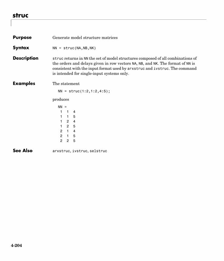
struc
4-204
4strucPurpose Generate model structure matrices
Syntax NN = struc(NA,NB,NK)
Description struc returns in NN the set of model structures composed of all combinations of the orders and delays given in row vectors NA, NB, and NK. The format of NN is consistent with the input format used by arxstruc and ivstruc. The command is intended for single-input systems only.
Examples The statement
NN = struc(1:2,1:2,4:5);
produces
NN = 1 1 4 1 1 5 1 2 4 1 2 5 2 1 4 2 1 5 2 2 5
See Also arxstruc, ivstruc, selstruc
timestamp
4-205
4timestampPurpose Allow bookkeeping of created objects
Syntax timestamp(obj)ts = timestamp(obj)
Description obj is any idmodel, iddata, or idfrd object. timestamp returns or displays a string with information about when the object was created and last modified.
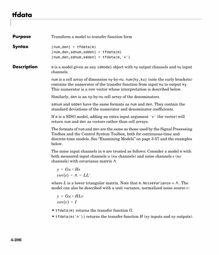
tfdata
4-206
4tfdataPurpose Transform a model to transfer function form
Syntax [num,den] = tfdata(m)[num,den,sdnum,sdden] = tfdata(m)[num,den,sdnum,sdden] = tfdata(m,'v')
Description m is a model given as any idmodel object with ny output channels and nu input channels.
num is a cell array of dimension ny-by-nu. num{ky,ku} (note the curly brackets) contains the numerator of the transfer function from input ku to output ky. This numerator is a row vector whose interpretation is described below.
Similarly, den is an ny-by-nu cell array of the denominators.
sdnum and sdden have the same formats as num and den. They contain the standard deviations of the numerator and denominator coefficients.
If m is a SISO model, adding an extra input argument 'v' (for vector) will return num and den as vectors rather than cell arrays.
The formats of num and den are the same as those used by the Signal Processing Toolbox and the Control System Toolbox, both for continuous-time and discrete-time models. See “Examining Models” on page 3-57 and the examples below.
The noise input channels in m are treated as follows: Consider a model m with both measured input channels u (nu channels) and noise channels e (ny channels) with covariance matrix
where L is a lower triangular matrix. Note that m.NoiseVariance = . The model can also be described with a unit variance, normalized noise source v:
• tfdata(m) returns the transfer function G.
• tfdata(m('n')) returns the transfer function H (ny inputs and ny outputs).
Λ
y Gu He+=cov e( ) Λ LL ′= =
Λ
y Gu HLv+=cov v( ) I=
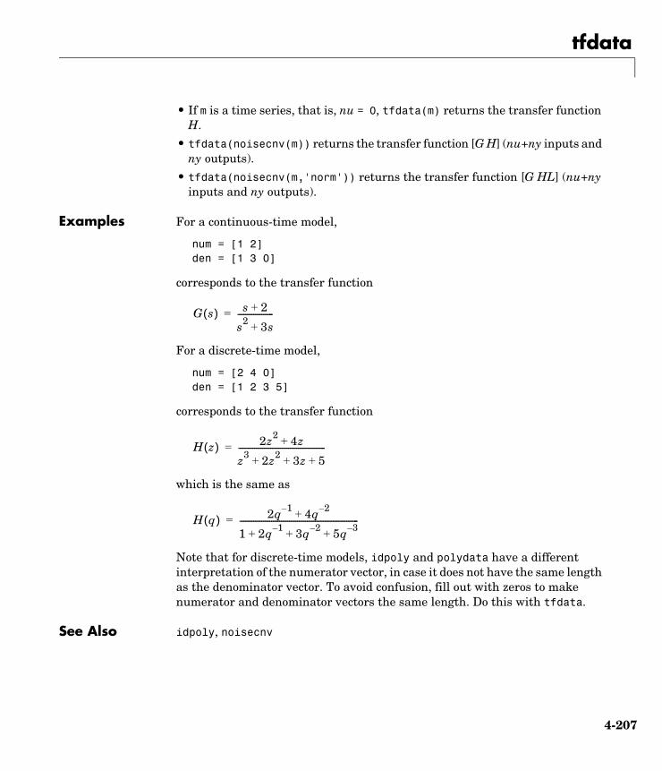
tfdata
4-207
• If m is a time series, that is, nu = 0, tfdata(m) returns the transfer function H.
• tfdata(noisecnv(m)) returns the transfer function [G H] (nu+ny inputs and ny outputs).
• tfdata(noisecnv(m,'norm')) returns the transfer function [G HL] (nu+ny inputs and ny outputs).
Examples For a continuous-time model,
num = [1 2]den = [1 3 0]
corresponds to the transfer function
For a discrete-time model,
num = [2 4 0]den = [1 2 3 5]
corresponds to the transfer function
which is the same as
Note that for discrete-time models, idpoly and polydata have a different interpretation of the numerator vector, in case it does not have the same length as the denominator vector. To avoid confusion, fill out with zeros to make numerator and denominator vectors the same length. Do this with tfdata.
See Also idpoly, noisecnv
G s( ) s 2+
s2 3s+------------------=
H z( ) 2z2 4z+
z3 2z2 3z 5+ + +--------------------------------------------=
H q( ) 2q 1– 4q 2–+
1 2q 1– 3q 2– 5q 3–+ + +------------------------------------------------------------=
view
4-208
4viewPurpose Plot a variety of model characteristics (requires the Control System Toolbox)
Syntax view(m)view(m('n'))view(m1,...,mN,Plottype)view(m1,PlotStyle1,...,mN,PlotStyleN)
Description m is the output-input data to be graphed, given as any idfrd or idmodel object. After appropriate model transformations, the LTI viewer of the Control System Toolbox is invoked. This allows bode, nyquist, impulse, step, and zero/poles plots.
To compare several models m1,...,mN, use view(m1,...,mN). With PlotStyle, the color, line style, and marker of each model can be specified.
view(m1,'y:*',m2,'b')
Adding Plottype as a last argument specifies the type of plot in which view is initialized. Plottype is any of 'impulse', 'step', 'bode', 'nyquist', 'nichols', 'sigma', or 'pzmap'. It can also be given as a cell array containing any collection of these strings (up to 6) in which case a multiplot is shown.
view does not display confidence regions. For that, use bode, nyquist, impulse, step, and pzmap.
The noise input channels in m are treated as follows: Consider a model m with both measured input channels u (nu channels) and noise channels e (ny channels) with covariance matrix
where L is a lower triangular matrix. Note that m.NoiseVariance = . The model can also be described with a unit variance, normalized noise source v:
• view(m) plots the characteristics of the transfer function G.
Λ
y Gu He+=
cov e( ) Λ LLT= =
Λ
y Gu HLv+=cov v( ) I=
view
4-209
• view(m('n')) plots the characteristics of the transfer function HL (ny inputs and ny outputs). The input channels have names v@yname, where yname is the name of the corresponding output.
• If m is a time series, that is, nu = 0, view(m) plots the characteristics of the transfer function HL.
• view(noisecnv(m)) plots the characteristics of the transfer function [G H] (nu+ny inputs and ny outputs). The noise input channels have names e@yname, where yname is the name of the corresponding output.
• view(noisecnv(m,'norm')) plots the characteristics of the transfer function [G HL] (nu+ny inputs and ny outputs). The noise input channels have names v@yname, where yname is the name of the corresponding output.
view does not give access to all of the features of ltiview. Use
ml = ss(m), ltiview(Plottype,ml,...)
to reach these options.
See Also bode, impulse, nyquist, step, pzmap
zpkdata
4-210
4zpkdataPurpose Compute zeros, poles, and transfer function gains of models
Syntax [z,p,k] = zpkdata(m)[z,p,k,dz,dp,dk] = zpkdata(m)[z,p,k,dz,dp,dk] = zpkdata(m,'v')
Description m is a model given as any idmodel object with ny output channels and nu input channels.
z is a a cell array of dimension ny-by-nu. z{ky,ku} (note the curly brackets) contains the zeros of the transfer function from input ku to output ky. This is a column vector of possibly complex numbers.
Similarly, p is an ny-by-nu cell array containing the poles.
k is a ny-by-nu matrix whose ky-ku entry is the transfer function gain of the transfer function from input ku to output ky. Note that the transfer function gain is the value of the leading coefficient of the numerator when the leading coefficient of the denominator is normalized to 1. It thus differs from the static gain. The static gain can be retrieved as Ks = freqresp(m,0).
dz contains the covariance matrices of the zeros in the following way: dz is a ny-by-nu cell array. dz{ky,ku} contains the covariance information about the zeros of the transfer function from ku to ky. It is a 3-D array of dimension 2-by-2-by-Nz, where Nz is the number of zeros. dz{ky,ku}(:,:,kz) is the covariance matrix of the zero z{ky,ku}(kz), so that the 1-1 element is the variance of the real part, the 2-2 element is the variance of the imaginary part, and the 1-2 and 2-1 elements contain the covariance between the real and imaginary parts.
dp contains the covariance matrices of the poles in the same way.
dk is a matrix containing the variances of the elements of k.
If m is a SISO model, adding an extra input argument 'v' (for vector) returns z and p as vectors rather than cell arrays.
Note that the zeros and the poles are associated with the different channel combinations. To obtain the so-called transmission zeros, use tzero.
zpkdata
4-211
The noise input channels in m are treated as follows: Consider a model m with both measured input channels u (nu channels) and noise channels e (ny channels) with covariance matrix
where L is a lower triangular matrix. Note that m.NoiseVariance = . The model can also be described with a unit variance, normalized noise source v.
Then,
• zpkdata(m) returns the zeros and poles of G.
• zpkdata(m('n')) returns the zeros and poles of H (ny inputs and ny outputs).
• If m is a time series, that is, nu = 0, zpkdata(m) returns the zeros and poles of H.
• zpkdata(noisecnv(m)) returns the zeros and poles of the transfer function [G H] (nu+ny inputs and ny outputs).
• zpkdata(noisecnv(m,'norm')) returns the zeros and poles of the transfer function [G HL] (nu+ny inputs and ny outputs).
The procedure handles both models in continuous and discrete time.
Note that you cannot rely on information about zeros and poles at the origin and at infinity for discrete-time models. (This is a somewhat confusing issue anyway.)
Algorithm The poles and zeros are computed using ss2zp. The covariance information is computed using the Gauss approximation formula, using the parameter covariance matrix contained in m. When the transfer function depends on the parameters, numerical differentiation is applied. The step sizes for the differentiation are determined in the M-file nuderst.
Λ
y Gu He+=cov e( ) Λ LL ′= =
Λ
y Gu HLv+=cov v( ) I=

zpkdata
4-212
Index-1
Index
Aadaptive noise cancelling 4-165adaptive parameter estimation 3-85advanced algorithm options 4-18advice
help facility 3-3model validation 3-70
AIC, the Akaike Information Criteriondefinition 3-72formal derivation 4-12
Akaike’s Final Prediction Error (FPE) 3-71AR model
estimation 3-29estimation techniques 3-93
ARARMAX structure 3-13ARMAX model
definition 2-29equation 3-12GUI 2-28
ARX modelcompare many 3-70GUI 2-26
Bbasic tools 3-3BJ 2-29Bode diagram 2-35Bode plot 1-10Box-Jenkins model
definition 3-12equation 2-29GUI 2-28
Burg’s methodAR command 3-93AR option 3-30
Cchannels
noise 3-60selection 3-79
closed-loop system 3-83communication window ident 2-2comparing different models 3-77comparisons using compare 3-59complex-valued data 3-107confidence region
for model validation 3-76GUI 2-34show in plots 3-65
continuous-time model 3-46as idss object 3-46estimation 3-68estimation options 3-54spectrum 3-104transformations 3-68
Control System Toolbox 3-95correlation analysis 1-4correlation between residuals and inputs 3-84covariance matrix
estimation 3-31in c2d/d2c 3-69suppressing calculation 3-100
covariance method 3-30creating models from data 2-2cross correlation function 1-17cross spectrum 3-15cross validation
by simulation 3-75relation to AIC, FPE 3-71
customized plots 2-43
Index
Index-2
Ddata
channels 3-24feedback (impulse response) 3-73feedback (limitations) 3-83feedback (testing) 3-84frequency domain 3-22frequency response 3-22missing data 3-82multiple experiments 3-25
Data Board 2-3data handling checklist 2-14data ranges 2-13data representation 2-7data views 1-4deadtime 3-41delays
definition 3-11delayest 3-84estimating 3-73in d2c 3-69use of nk 3-78
detrending data 2-12difference equation 1-7disturbance 1-6disturbance spectra 2-35drift matrix 3-86dynamic models, introduction 1-6
Eempirical transfer function estimate 3-21enumeration of parameters 3-106estimation
nonparametric 3-19parametric 3-28
estimation data 1-4
estimation focusalgorithm property 4-14continuous time model 3-55in GUI 2-13prefiltering 3-82
estimation methoddirect 2-17instrumental variables 3-17nonparametric 3-19parametric (basic commands) 3-28parametric (GUI) 2-17prediction error approach 2-24
exporting to the MATLAB workspace 2-39extended least squares (ELS) 3-89
Ffault detection 3-90feedback 1-15feedback in data
impulse response 3-73limitations 3-83testing 3-84
filtering datafor model quality 3-82
fixed parameter 4-16focus
algorithm property 4-14continuous time model 3-55in GUI 2-13prefiltering 3-82
forgetting factor 3-87FPE 3-72frequency
function (definition) 3-9function (GUI) 2-18plots 3-9
Index
Index-3
range 3-9resolution (in spa) 4-192resolution (in spafdr) 4-195resolution(concept) 3-22response 2-18scales 3-9
frequency domaindata 3-22description 3-11initial state 3-99
frequency function 3-10frequency response
concept 1-10data (idfrd object) 3-22function 3-10graph 3-66
GGauss-Newton direction 4-18Gauss-Newton minimization 3-31geometric lattice method
AR command 3-93AR option 3-30
graphical user interface (GUI) 2-2greybox-modeling 3-51GUI 2-2
topics 2-41
HHamming window 3-21HARF method 3-89
Iidarx model object 3-43
ident window 2-41identification method
instrumental variables 3-17nonparametric 3-19parametric 3-28prediction error approach 2-24subspace 2-31
identification process, basic steps 1-12idfrd model object 3-20
as data information 3-22as estimated model 3-63
idgrey model object 3-51idpoly model object 3-40idproc model object 3-41idss model object 3-46impulse response
concept 1-10definition 3-10
Information Theoretic Criterion (AIC) 3-71initial condition 3-31initial parameter values
iterative search 3-54startup models 3-97
initial state 3-98frequency domain 3-99in GUI 2-21, 2-25state space model 3-47
innovations form 3-13input signals 1-6instrumental variable 3-17
IV4 method 3-29IVAR method 3-30
iterative search 3-31local minima 3-97use in pem 3-103
Index
Index-4
KKalman filter 3-86Kalman gain 3-14
Llag window
definition 3-16in spa 3-21
layout 2-42least mean squares (LMS) 3-88least squares 2-27Levenberg-Marquard 4-18LimitError 4-17linear regression
recursive algorithms 3-85using ARX 3-102
linear trends 3-81linestyles 3-65local minima 3-97loss function 3-105
Mmain ident window 2-41markers 3-65maximum likelihood
criterion 3-33method 3-17
MaxIter 4-18MaxSize 4-16memory horizon 3-87merge experiments 3-25Minimum Description Length (MDL) 3-72missing data 3-82model
continuous-time 3-46
continuous-time (estimation optiond) 3-54continuous-time (spectrum) 3-104continuous-time(transformations) 3-68nonparametric 3-11output-error 1-8parametric 2-22properties 1-10set 1-4state-space 1-8structure 2-22uncertainty 3-75view functions 2-33views 1-8
Model Board 2-3model error model 3-74model order 1-7model structure 1-4model uncertainty
GUI 2-34show in plots 3-65
model validationavailable methods 3-70definition 1-5
model views 1-4modified covariance method 3-93multi-output models
criterion 3-32multiple experiments 3-25multivariable ARX model 3-43multivariable systems
definition 1-18loss function 3-105model structures 3-77
multivariate signals 3-93
Index
Index-5
NN4Horizon 3-36N4Weight 3-35na,nb,nc,nd,nf
parameter definitions 3-11noise 1-6noise channels 3-60noise model 1-8noise source 1-9noise-free simulation
concept 1-9for model validation 3-75
nonequal sampling 3-25nonparametric estimation 3-19nonparametric identification 1-4Normalized Gradient (NG) Approach 3-88numerical differentiation
for gradients 3-54for transformations 3-69
Nyquist frequency 3-104Nyquist plot 3-21
OOE 2-29offset levels 3-81offsets 3-81online algorithms 3-85order editor 2-24outliers 3-81
feedback 3-74signals 1-4
output feedback 3-74output signals 1-6output-error model
definition 1-8equation 2-29
GUI 2-28prediction 3-59state space model 3-47
Pparametric identification 1-4parametric model 2-22parametric model estimation 3-28periodic input 3-94periodogram
etfe for time series 3-92from etfe 3-22
physical equilibrium, 3-81pole
concept 1-11GUI 2-36
pole-zero cancellation 3-73poorly damped systems 1-18prediction 3-58
error identification 2-24error method 3-17k step ahead 3-59
prediction errordefinition 3-16pe command 3-59
preferencesin GUI 2-43
prefilteringfor model quality 3-82in GUI 2-13
process model 3-31idproc 3-41
QQuickstart menu item 2-14

Index
Index-6
Rrandom walk 3-86recursive identification
basic algorithms 3-85commands 3-4pseudo-linear regression approach 3-89
reference list 1-21regression vector 3-85resampling 2-14residual analysis
concept 1-17resid command 3-73
residuals 1-2resolution
concept 3-22in spa 4-192in spafdr 4-195
robustified criterionagainst outliers 3-81in linear regression 3-103LimitError 4-17relation to loss function 3-105
Ssampling interval 1-6SearchDirection 4-18segmentation problem 3-90sequential estimation 3-85sessions (GUI) 2-5SHARF method 3-89shift operator 2-29simulating data 2-15simulation
concept 3-58noise level 3-105
spectral analysis
concept 1-4time series 3-92
spectral density 3-104spectrum 3-9spectrum normalization 3-103startup identification procedure 1-14state space model
output-error model 3-47state variable 1-8state vector 3-13state-space model
continuous time 3-14definition 1-7equation 3-13GUI 2-30stochastic 3-14
step responseconcept 1-10
structure 1-4structure matrices 3-48subspace method 2-31
Ttesting for feedback 3-84time constant 3-41time delay
definition 1-7in idproc 3-41
time domain description 3-10time series model
prediction 3-59spectral estimation 3-21
time series modelinggeneral remarks 3-92
time-continuous systems 3-40tolerance 4-18

Index
Index-7
trace 3-31transfer function
concept 1-8definition 3-10
transformations of noise models 3-105transient response 1-10
graph 3-66
Uuncertainty
parameter free state-space model 3-76suppressing calculation 3-100
Unnormalized Gradient (UG) Approach 3-88
Vvalidation data 1-2
Wwhite noise 1-9window sizes 3-21working data 1-4Working Data set 2-4
YYule-Walker approach
AR command 3-93AR option 3-30
Zzero
concept 1-11GUI 2-36
zero-pole format 3-64
zeros and polesgraph 3-66