System Identi cation through Online Sparse Gaussian Process Regression with...

System Identification through Online Sparse GaussianProcess Regression with Input Noise

Hildo Bijl [email protected] Center for Systems and ControlDelft University of TechnologyDelft, The Netherlands

Thomas B. Schon [email protected] of Information TechnologyUppsala UniversityUppsala, Sweden

Jan-Willem van Wingerden [email protected] Center for Systems and ControlDelft University of TechnologyDelft, The Netherlands

Michel Verhaegen [email protected]

Delft Center for Systems and Control

Delft University of Technology

Delft, The Netherlands

Abstract

There has been a growing interest in using non-parametric regression methods like GaussianProcess (GP) regression for system identification. GP regression does traditionally havethree important downsides: (1) it is computationally intensive, (2) it cannot efficientlyimplement newly obtained measurements online, and (3) it cannot deal with stochastic(noisy) input points. In this paper we present an algorithm tackling all these three issuessimultaneously. The resulting Sparse Online Noisy Input GP (SONIG) regression algorithmcan incorporate new noisy measurements in constant runtime. A comparison has shownthat it is more accurate than similar existing regression algorithms. When applied tononlinear black-box system modeling, its performance is competitive with existing nonlinearARX models.

Keywords: Nonlinear system identification, Gaussian processes, regression, machinelearning, sparse methods.

1. Introduction

The Gaussian Process (GP) (Rasmussen and Williams, 2006) has established itself as astandard model for nonlinear functions. It offers a representation that is non-parametricand probabilistic. The non-parametric nature of the GP means that it does not rely onany particular parametric functional form to be postulated. The fact that the GP is aprobabilistic model means that it is able to take uncertainty into account in every aspect ofthe model.

c©2017 Hildo Bijl, Thomas B. Schon, Jan-Willem van Wingerden, Michel Verhaegen.

Bijl

The nonlinear system identification problem amounts to learning a nonlinear mathe-matical model based on data that is observed from a dynamical phenomenon under study.Recently there has been a growing interest of using the GP to this end and it has in factallowed researchers to successfully revisit the linear system identification problem and estab-lish new and significantly improved results on the impulse estimation problem (Pillonettoand De Nicolao, 2010; Pillonetto et al., 2011; Chen et al., 2012). There are also older resultson nonlinear ARX type models (Kocijan et al., 2005) and new results on the nonlinear statespace models based on the GP (Svensson and Schon, 2017; Frigola et al., 2013, 2014). Wealso mention the nice overview by Kocijan (2016).

When the basic GP model is used for regression, it results in a computational complexitythat is too high to be practically useful, stochastic inputs cannot be used and it cannot beused in an online fashion. These three fundamental problems of basic GP regression havebeen addressed in many different ways, which we return to in Section 2. The nonlinearsystem identification problem typically requires us to solve these three problems simulta-neously. This brings us to our two main contributions of this paper. (1) We derive analgorithm allowing us to—in an online fashion—include stochastic training points to oneof the classic sparse GP models, the so-called FITC (Fully Independent Training Condi-tional) algorithm. (2) We adapt the new algorithm to the nonlinear system identificationproblem, resulting in an online algorithm for nonlinear system identification. The experi-mental results show that the our new algorithm is indeed competitive compared to existingsolutions.

The system identification formulation takes inspiration from the nonlinear autoregressivemodel with exogenous (ARX) inputs of the following form

yk = φ(yk−1, . . . ,yk−ny ,uk−1, . . . ,uk−nu), (1)

where φ(·) denotes some nonlinear function of past inputs uk−1, . . . ,uk−nu and past out-puts yk−1, . . . ,yk−ny to the system. To this end we develop a non-parametric and proba-bilistic GP model which takes the following vector

xk = (yk−1, . . . ,yk−ny ,uk−1, . . . ,uk−nu), (2)

as its input vector. The crucial part behind our solution from a system identification pointof view is that we continuously keep track of the covariances between respective outputestimates yk, . . . ,yk−ny and inputs uk, . . . ,uk−nu . Every time we incorporate new trainingdata, the respective means and covariances of these parameters are further refined.

The paper is organized as follows. Section 2 starts by examining three important ex-isting problems within GP regression, giving a quick summary of the solutions discussed inliterature. In Section 3 we expand on these methods, enabling GP regression to be appliedin an online manner using noisy input points. This results in the basic version of the newalgorithm. Section 4 subsequently outlines various ways of extending this algorithm, allow-ing it to be applied to system identification problems. Experimental results, first for thebasic algorithm (Algorithm 1) and then for its system identification set-up (Algorithm 2)are shown in Section 5. Section 6 finally gives conclusions and recommendations for futurework along this direction.

2

System Identification through Online Sparse Gaussian Process Regression with Input Noise

2. Backgrounds and limitations of Gaussian process regression

Gaussian process regression is a powerful regression method but, like any method, it hasits limitations. In this section we look at its background, what exact limitations it has andwhat methods are available in literature to tackle these. Also the assumptions made andthe notation used is introduced.

2.1 Regular Gaussian process regression

GP regression (Rasmussen and Williams, 2006) is about approximating a function f(x)through a number of n training points (measurements) (x1, y1), (x2, y2), . . . , (xn, yn). Here,x denotes the training input point and y the measured function output. (For now we assumescalar outputs. Section 4.1 looks at the multi-output case.) We assume that the trainingoutputs are corrupted by noise, such that yi = f(xi) + ε, with ε ∼ N (0, σ2n) being Gaussianwhite noise with zero mean and variance σ2n.

As shorthand notation, we merge all the training points xi into a training set X andall corresponding output values yi into an output vector y. We now write the noiselessfunction output f(X) as f , such that y = f + ε, with ε ∼ N (0,Σn) and Σn = σ2nI.

Once we have the training data, we want to predict the function value f(x∗) at a specifictest point x∗. Equivalently, we can also predict the function values f∗ = f(X∗) at a wholeset of test points X∗. To accomplish this using GP regression, we assume that f∗ and fhave a prior joint Gaussian distribution given by[

f0

f0∗

]∼ N

([m(X)m(X∗)

],

[k(X,X) k(X,X∗)k(X∗, X) k(X∗, X∗)

])= N

([mm∗

],

[K K∗KT

∗ K∗∗

]), (3)

where in the second part of the equation we have introduced another shorthand notation.Note here that m(x) is the prior mean function for the Gaussian process and k(x,x′) isthe prior covariance function. The superscript 0 in f0 and f0

∗ also denotes that we arereferring to the prior distribution: no training points have been taken into account yet. Inthis paper we make no assumptions on the prior mean/kernel functions, but our exampleswill apply a zero mean function m(x) = 0 and a squared exponential covariance function

k(x,x′) = α2 exp

(−1

2

(x− x′

)TΛ−1

(x− x′

)), (4)

with α a characteristic output length scale and Λ a diagonal matrix of characteristic inputsquared length scales. For now we assume that these hyperparameters are known, but inSection 4.3 we look at ways to tune them.

From (3) we can find the posterior distribution of both f and f∗ given y as[fn

fn∗

]∼ N

([µn

µn∗

],

[Σn Σn

∗(Σn

∗ )T Σn∗∗

]),[

µn

µn∗

]=

[(K−1 + Σ−1

n

)−1 (K−1m+ Σ−1

n y)

m∗ +KT∗ (K + Σn)−1 (y −m)

],

[Σn Σn

∗(Σn

∗ )T Σn∗∗

]=

[ (K−1 + Σ−1

n

)−1Σn (K + Σn)−1K∗

KT∗ (K + Σn)−1 Σn K∗∗ −KT

∗ (K + Σn)−1K∗

]. (5)

3

Bijl

Note here that, while we use m and K to denote properties of prior distributions, we useµ and Σ for posterior distributions. The superscript n indicates these are posteriors takingn training points into account, and while a star ∗ subscript denotes a parameter of the testset, an omitted subscript denotes a training parameter.

2.2 Sparse Gaussian process regression

An important limitation of Gaussian process regression is its computational complexityof O(n3), with n the number of training points. This can be tackled through parallelcomputing (Gal et al., 2014; Deisenroth and Ng, 2015) but a more common solution is touse the so-called sparse methods. An overview of these is given by Candela and Rasmussen(2005), summarizing various contributions (Smola and Bartlett, 2001; Csato and Opper,2002; Seeger et al., 2003; Snelson and Ghahramani, 2006b) into a comprehensive framework.With these methods, and particularly with the FITC method that we will apply in thispaper, the runtime can be reduced to being linear with respect to n, with only a limitedreduction in how well the available data is being used.

All these sparse methods make use of so-called inducing input points Xu to reduce thecomputational complexity. Such inducing input points are also used in the more recent workon variational inference (Titsias, 2009; Titsias and Lawrence, 2010). However, as pointedout by McHutchon (2014), these points are now not used for the sake of computational speedbut merely as ‘information storage’. McHutchon (2014) also noted that the correspondingmethods have a large number of parameters to optimize, making the computation of thederivatives rather slow. Furthermore, even though variations have been developed which doallow the application of variational inference to larger data sets (Hensman et al., 2013; Galet al., 2014; Damianou et al., 2016), online methods generally require simpler and fastermethods, like the NIGP (Noisy Input GP) method from McHutchon and Rasmussen (2011),which is what we will focus on.

To apply sparse GP regression, we first find the posterior distribution of the inducingoutputs fu at the corresponding inducing input points Xu. This can be done in O(n3) timethrough (5) (replacing f∗ by fu) or in O(nn2u) time through the FITC regression equation[

fn

fnu

]∼ N

([µn

µnu

],

[Σn Σn

u

(Σnu)T Σn

uu

]),[

µn

µnu

]=

[m+ ΣnΣ−1

n (y −m)

mu + (Σnu)T

(Λ−1n + Σ−1

n

)(y −m)

],

Σn =(Λ−1n + Σ−1

n

)−1+ Σn (Λn + Σn)−1Ku∆−1KT

u (Λn + Σn)−1 Σn,

Σnu = Σn (Λn + Σn)−1Ku∆−1Kuu,

Σnuu = Kuu∆−1Kuu. (6)

Here we have used the shorthand notation ∆ = Kuu + KTu (Λn + Σn)−1Ku and Λn =

diag(K −KT

uK−1uuKu

), with diag being the function that sets all non-diagonal elements of

the given matrix to zero. The FITC regression equation is an approximation, based on theassumption that all function values f(x1), . . . , f(xn) are (a priori) independent given fu.

Once we know the distribution of fu, we calculate the posterior distribution of f∗.Mathematically, this method is equivalent to assuming that f and f∗ are conditionally

4


independent, given fu. It follows that[fnu

fn∗

]∼ N

([µnu

µn∗

],

[Σnuu Σn

u∗Σn∗u Σn

∗∗

]),[

µnu

µn∗

]=

[µnu

m∗ +K∗uK−1uu

(µnu −mu

)] ,[Σnuu Σn

u∗Σn∗u Σn

∗∗

]=

[Σnuu Σn

uuK−1uuKu∗

K∗uK−1uu Σn

uu K∗∗ −K∗uK−1uu (Kuu − Σn

uu)K−1uuKu∗

]. (7)

2.3 Online Gaussian process regression

A second limitation of GP regression is the difficulty with which it can incorporate newtraining points. For regular GP regression, a new measurement n+ 1 can be added to theexisting set of n training points through a matrix update, resulting in an O(n2) runtime.For sparse methods using inducing input (basis) points this can generally be done moreefficiently (Csato and Opper, 2002; Candela and Rasmussen, 2005; Ranganathan et al.,2011; Kou et al., 2013; Hensman et al., 2013). The main downside is that most methodsset requirements on these inducing input points. However, the FITC and the PITC (Par-tially Independent Training Conditional) methods can be set up in an online way withoutsuch constraints (Huber, 2013, 2014; Bijl et al., 2015). We briefly summarize the resultingalgorithm.

Suppose that we know the distribution of fu, given the first n training points. Thisis written as fn

u . Next, consider a new measurement (xn+1, yn+1), whose notation wewill shorten to (x+, y+). To incorporate it, we first predict the posterior distribution off+ = f(x+) based on only the first n training points. Identically to (7), this results in[

fnu

fn+

]∼ N

([µnu

µn+

],

[Σnuu Σn

u+

Σn+u Σn

++

]),[

µnu

µn+

]=

[µnu

m+ +K+uK−1uu

(µnu −mu

)] ,[Σnuu Σn

u+

Σn+u Σn

++

]=

[Σnuu Σn

uuK−1uuKu+

K+uK−1uu Σn

uu K++ −K+uK−1uu (Kuu − Σn

uu)K−1uuKu+

]. (8)

If we subsequently incorporate the new measurement, identically to (5), then we get[fn+1u

fn+1+

]∼ N

([µn+1u

µn+1+

],

[Σn+1uu Σn+1

u+

Σn+1+u Σn+1

++

]),[

µn+1u

µn+1+

]=

[µnu + Σn

u+

(Σn++ + σ2n

)−1 (y+ − µn+

)σ2n(Σn++ + σ2n

)−1µn+ + Σn

++

(Σn++ + σ2n

)−1y+

],[

Σn+1uu Σn+1

u+

Σn+1+u Σn+1

++

]=

[Σnuu − Σn

u+(Σn++ + σ2n)−1Σn

+u Σnu+(Σn

++ + σ2n)−1σ2nσ2n(Σn

++ + σ2n)−1Σn+u σ2n(Σn

++ + σ2n)−1Σn++

]. (9)

This expression (or at least the part relating to fu) is the update law for the FITC algorithm.It tells us exactly how the distribution of fn+1

u (both µn+1u and Σn+1

uu ) depends on x+ andy+. With this distribution, we can subsequently always find the distribution of new testpoint outputs f∗ in an efficient way through (7).

5

Bijl

2.4 Using stochastic input points

The third limitation is that the GP regression algorithm assumes that the input points aredeterministic. This assumption concerns both the training (measurement) points x and thetest points x∗. For noisy (stochastic) test points x∗, we can work around the problem byapplying moment matching (Deisenroth, 2010). This technique can subsequently also beexpanded for noisy training points (Dallaire et al., 2009), but the effectiveness is limitedbecause the method integrates over all possible a priori functions, and not over all possiblea posteriori functions. There are methods that include posterior distributions (Girard andMurray-Smith, 2003) but these often only work for noisy test points and not for noisy train-ing points. The NIGP algorithm (McHutchon and Rasmussen, 2011) is the only previouslyexisting algorithm that we are aware of that is include posterior distributions at the sametime as it can deal with noisy training points. This is the method we will be expandingupon in this paper.

It should be noted that the variational methods mentioned earlier can also deal withstochastic input points, up to a certain degree. However, as also mentioned before, theycannot do so as computationally efficient as the NIGP algorithm or the algorithm that wewill develop, so their applicability to online system identification remains limited. Addition-ally, it is also possible to take into account the effects of noisy training points by assumingthat the noise variance varies over the input space; a feature called heteroscedasticity. Thishas been investigated quite in-depth (Goldberg et al., 1997; Le and Smola, 2005; Wang andNeal, 2012; Snelson and Ghahramani, 2006a) but it would give more degrees of freedomto the learning algorithm than would be required, and as a result these methods have areduced performance for the problems we consider. We will not consider these methodsfurther in this paper.

3. Expanding the algorithm for stochastic training points

This section contains our main contribution: enabling the FITC algorithm to handlestochastic training points in an online way. From a computational point of view, the novelupdate laws given here are simple and efficient, relative to other methods.

3.1 The online stochastic measurement problem

Consider the case where we know the distribution fnu ∼ N

(µnu,Σ

nuu

)(initially we have

f0u ∼ N

(µ0u,Σ

0uu

)= N (mu,Kuu)) and we obtain a new measurement at some unknown

input point x+. As before, the true function output f+ = f(x+) is also unknown. Ourmeasurement only gives us values x+ and f+ approximating these and hence tells us thatx+ ∼ N (x+,Σ+x) and f+ ∼ N (f+,Σ+f

). (Note that f+ and y+ are identical, and so areΣ+f

and σ2n. For the sake of uniform notation, we have renamed them.) We assume thatthe noise on the input and the output is independent, and hence that x+ and f+ are apriori not correlated.

Our main goal is to find the posterior distribution fn+1u , given this stochastic training

point. This can be done through

p(fn+1u |x+, f+,f

nu ) =

∫Xp(fn+1

u |x+, x+, f+,fnu )p(x+|x+, f+,f

nu ) dx+. (10)

6


In the integral, the first probability p(fn+1u |x+, x+, f+,f

nu ) is the update law for fn+1

u if

x+ was known exactly. It directly follows from (9). The second probability p(x+|x+, f+,fnu )

is the posterior distribution of x+, given both fnu and the new measurement. Since this

latter term is more difficult to deal with, we examine it first.

3.2 The posterior distribution of the training point

The posterior distribution of x+ can be found through Bayes’ theorem,

p(x+|f+, x+,fnu ) =

p(f+|x+, x+,fnu )p(x+|x+,f

nu )

p(f+|x+,fnu )

. (11)

Here p(x+|x+,fnu ) = p(x+|x+) = N (x+,Σ+x) and p(f+|x+,f

nu ) equals an unknown

constant (i.e., not depending on x+). Additionally,

p(f+|x+, x+,fnu ) = p(f+|x+,f

nu ) = N

(µn+,Σ

n++ + Σ+f

), (12)

where µn+ and Σn++ follow from (8). Note that both these quantities depend on x+ in a

nonlinear way. Because of this, the resulting probability p(x+|f+, x+,fnu ) will be non-

Gaussian. To work around this problem, we have to make some simplifying assumptions.Similarly to Girard and Murray-Smith (2003), we linearize1 the Gaussian process f+ (whichdepends on x+) around a point x+. That is, we assume that

p(f+|x+,fnu ) = N

(µn+(x+) +

dµn+(x+)

dx+(x+ − x+) ,Σn

++(x+) + Σ+f

). (13)

In other words, we assume that the mean varies linearly with x+, while the covarianceis constant everywhere. This is a necessary assumption for p(x+|f+, x+,f

nu ) to have a

Gaussian solution. It follows as

p(x+|f+, x+,fnu ) = N

(xn+1+ ,Σn+1

+x

),

xn+1+ = x+ + Σn+1

+x

((dµn+(x+)

dx+

)T (Σn++(x+) + Σ+f

)−1

(dµn+(x+)

dx+(x+ − x+) +

(f+ − µn+(x+)

))),

Σn+1+ =

((dµn+(x+)

dx+

)T (Σn++(x+) + Σ+f

)−1(dµn+(x+)

dx+

)+ Σ−1

+x

)−1

. (14)

We are left to choose a linearization point x+. The above equation is easiest to apply when

we choose x+ = x+, but when(f+ − µn+(x+)

)is large, this may result in inaccuracies due

to the linearization. It is generally more accurate to choose x+ as xn+1+ . However, xn+1

+ isinitially unknown, so it may be necessary to apply the above equation multiple times, eachtime resetting x+ to the latest value of xn+1

+ that was found, to find the most accurateposterior distribution of x+.

1. Applying moment-matching like in Section 4.5 does not work here, since we would have to integrate overthe inverse of a matrix k(x,x) that depends on the integration parameter x.

7

Bijl

3.3 Updating the inducing input point function values

Using the above, we can solve (10). This is done by approximating the GP fu(x+) by itsTaylor expansion around xn+1

+ . Element-wise we write this as

fn+1ui

(x+) = fn+1ui

(xn+1+ ) +

dfn+1ui

(xn+1+ )

dx+

(x+ − xn+1

+

)+

1

2

(x+ − xn+1

+

)T d2fn+1ui

(xn+1+ )

dx2+

(x+ − xn+1

+

)+ . . . . (15)

Within this Taylor expansion, Girard and Murray-Smith (2003) made the assumption that

higher order derivatives like d2fnu

dx2+

are negligible, remaining with just a linearization of the

GP. We do not make this assumption, but instead assume that Σ2+x

and higher powers ofΣ+x are negligible. (If the uncertainties in x+ are so large that this assumption does nothold, then any form of Gaussian process regression is likely to fail.) This assumption is notonly more loose—resulting in an extra term in (15)—but it is also easier to verify.

An additional assumption we need to make is that x+ is independent of fu. This isreasonable, as x+ is only contaminated by Gaussian white noise. Applying this, we cansolve (10) through both (14) and (15). The result equals

fn+1u ∼ N

(µn+1u ,Σn+1

uu

),

µn+1ui

= µn+1ui

(xn+1+ ) +

1

2tr

(d2µn+1

ui(xn+1

+ )

dx2+

Σn+1+x

),

Σn+1uiuj

= Σn+1uiuj

(xn+1+ ) +

(dµn+1

uj(xn+1

+ )

dx+

)Σn+1+x

(dµn+1

ui(xn+1

+ )

dx+

)T

+1

2tr

((d2Σn+1

uiuj(xn+1

+ )

dx2+

)Σn+1+x

). (16)

Here, the functions µn+1ui

(x+) and Σn+1uiuj

(x+) (for a given point x+) are given by (9),combined with (8). Finding all the derivatives of these parameters can be a daunting task,especially for non-scalar inputs x+, but the mathematics are relatively straightforward, sofor this we refer to the Appendix.

It is interesting to compare expression (16) with what was used by McHutchon andRasmussen (2011) in their NIGP algorithm. They did not include the term involvingd2µn+1

ui/dx2

+. Later on, in Section 5.1, we will find that exactly this term causes the newalgorithm to perform better than the NIGP algorithm. As such, the above update law (16)also serves as an improvement with respect to the NIGP algorithm.

3.4 The SONIG algorithm

Applying the equations developed so far is done through the Sparse Online Noisy Input GP(SONIG) algorithm, outlined in Algorithm 1. This algorithm is computationally efficient,in the sense that a single updating step (incorporating one training point) can be done inconstant runtime with respect to the number of training points already processed. The

8


runtime does depend on the number of inducing input points through O(n3u), just like itdoes for all sparse GP regression algorithms.

Input:A possibly expanding set of training points (x1, y1), . . . , (xn, yn) in which both xand y are distorted by Gaussian white noise.

Preparation:Either choose the hyperparameters based on expert knowledge, or apply theNIGP hypertuning methods of McHutchon and Rasmussen (2011) on a subset ofthe data (a few hundred points) to find the hyperparameters.Optionally, apply the NIGP regression methods on this subset of data to obtainan initial distribution of fu. Otherwise, initialize fu as N (mu,Kuu).

Updating:while there are unprocessed training points (xn+1, yn+1) do

1. Apply (14) to find the posterior distribution of the training point xn+1

(written as x+).2. Use (16) to update the distribution of fu.3. Optionally, use (17) and (18) to calculate the posterior distribution of thefunction value f(x+) (written as f+).

end

Prediction:Apply (7) to find the distribution f∗ for any set of deterministic test points. Forstochastic test points, use the expansion from Section 4.5.

Algorithm 1: The Sparse Online Noisy Input GP (SONIG) algorithm: an online versionof the FITC algorithm capable of dealing with stochastic (noisy) training points.

4. Extensions of the SONIG algorithm

In the previous section we have presented the basic idea behind the SONIG algorithm. Thereare various further extensions that can be derived and implemented in the algorithm. Forinstance, the algorithm can deal with multi-output functions f(x) (Section 4.1), it can giveus the posterior distribution of the output f+ as well as its correlation with the input x+

(Section 4.2), we can implement hyperparameter tuning (Section 4.3), we can add inducinginput points online (Section 4.4) and we can make predictions f∗ using stochastic test pointsx∗ (Section 4.5). Many of these extensions are necessary to apply the SONIG algorithmfor system identification. The resulting system identification algorithm is summarized inAlgorithm 2.

4.1 Multiple outputs

So far we have approximated functions f(x) with only one output. It is also possible toapproximate functions f(x) with dy > 1 outputs. A common way in which this is donein GP regression algorithms (Deisenroth and Rasmussen, 2011; Alvarez et al., 2012) is byassuming that, given a deterministic input x, all outputs f1(x), . . . , fdy(x) are independent.

9

Bijl

With this assumption, it is possible to keep a separate inducing input point distributionf iu ∼ N

(µiu,Σ

iu

)for each output fi(x). Hence, each output is basically treated separately.

When using stochastic input points (again, see Deisenroth and Rasmussen (2011)) theoutputs do become correlated. We now have two options. If we take this correlation into

account, we have to keep track of the joint distribution of the vectors f1u, . . . ,f

dyu , effectively

merging them into one big vector. This results in a vector of size nudy, giving our algorithm acomputational complexity of O(n3ud

3y). Alternatively, we could also neglect the correlation

between the inducing input point distributions f iu caused by stochastic training points

x+ ∼ N (x+,Σ+x). If we do, we can continue to treat each function output separately,giving our algorithm a runtime of O(n3udy). Because one of our aims in this paper is toreduce the runtime of GP regression algorithms, we will apply the second option.

When each output is treated separately, each output also has its own hyperparameters.Naturally, the prior output covariance α2

i and the output noise σ2nican differ per output f i,

but also the input length scales Λi may be chosen differently for each output. In fact, it iseven possible to specify a fully separate covariance function ki(x,x

′) per output f i, thoughin this paper we stick with the squared exponential covariance function.

Naturally, there are a few equations which we should adjust slightly in the case ofmultivariate outputs. In particular, in equation (14), the parameter Σn

++(x+) would notbe a scalar anymore, but become a matrix. Due to our assumption that the outputs areindependent, it would be a diagonal matrix. Similarly, the derivative dµn+/dx+ would notbe a row vector anymore. Instead, it would turn into the matrix dµn

+/dx+. With theseadjustments, (14) still holds and all other equations can be applied as usual.

4.2 The posterior distribution of the measured output

In Section 3.3 we found the posterior distribution for fu. For some applications (like thesystem identification set-up presented in Section 5.2) we also need the posterior distributionof the measured function value f+, even though we do not exactly know to which input itcorresponds. We can find this element-wise, using the same methods, through

E[f+]i = µn+1+i

(xn+1+ ) +

1

2tr

(d2µn+1

+i(xn+1

+ )

dx2+

Σn+1+x

),

V[f+,f+]i,j = Σn+1+i+j

(xn+1+ ) +

(dµn+1

+i(xn+1

+ )

dx+

)Σn+1+x

(dµn+1

+j(xn+1

+ )

dx+

)T

+1

2tr

((d2Σn+1

+i+j(xn+1

+ )

dx2+

)Σn+1+x

). (17)

Note here that Σn+1++ (xn+1

+ ) is (by assumption) a diagonal matrix, simplifying the aboveequation for non-diagonal terms. As such, the covariance between two different functionoutputs f+i and f+j only depends on the second term in the above expression.

It may occur that we also need to know the posterior covariance between the functionvalue f+ and the function input x+. Using the same method, we can find that

V[f+,x+] =

(dµn+1

+ (xn+1+ )

dx+

)Σn+1+x

. (18)

10


This allows us to find the joint posterior distribution of x+ and f+.

4.3 Applying hyperparameter tuning to the algorithm

So far we have assumed that the hyperparameters of the Gaussian process are known apriori. When this is not the case, they need to be tuned first. While this could be doneusing expert knowledge of the system, it can also be done automatically.

McHutchon and Rasmussen (2011), with their NIGP method, offer an effective methodof tuning the hyperparameters, which also tells us the input noise variance Σ+x . However,this method has a computational complexity of O(n3), with n still the number of trainingpoints. As such, it can only be used for a small number of measurements and it cannot beused online. Hence NIGP does not seem to be applicable to our problem.

However, Chalupka et al. (2013) compare various GP regression algorithms, includingmethods to tune hyperparameters. One of their main conclusions is that the subset-of-data(SoD) method provides a good trade-off between computational complexity and predictionaccuracy. When using the SoD method, we do not apply hyperparameter tuning to our fulldata set, of possibly tens of thousands of input-output pairs. Instead, we randomly take asubset (say, a few hundred) of these data points and tune the hyperparameters only basedon this selection. For this latter step any suitable hyperparameter tuning algorithm can beused, although we use the NIGP method described by McHutchon and Rasmussen (2011).

Chalupka et al. (2013) also conclude that, for the regression problem with known hy-perparameters, the FITC algorithm provides a very good trade-off between complexity andaccuracy. So after having tuned the hyperparameters, it will be an effective choice to usethe online FITC algorithm with stochastic training points (that is, the SONIG algorithm)as our regression method.

4.4 Adjusting the set of inducing input points online

When using an online GP regression algorithm, it is often not known in advance what kindof measured input points x the system will get. As such, choosing the inducing input pointsXu in advance is not always possible, nor wise. Instead, we can adjust the inducing inputpoints while the algorithm is running. There are ways to fully tune the set of inducinginput points, like using the latent variable methods by Titsias (2009); Titsias and Lawrence(2010), but those methods require the optimization of many parameters, resulting in acomputationally complex procedure. To keep the required computations limited, we haveto opt for a simpler method and add/remove inducing input points based on areas of theinput space we are interested in or have data at.

Suppose that we denote the current set of inducing input points by Xu, and that wewant to add an extra set of inducing input points Xu+ . In this case, given all the data that

11

Bijl

we have, the distributions of fu and fu+ satisfy, identically to (7),[fufu+

]∼ N

([µu

µu+

],

[Σuu Σuu+

Σu+u Σu+u+

]),[

µu

µu+

]=

[µu

mu+ +Ku+uK−1uu (µu −mu)

],[

Σnuu Σn

uu+

Σnu+u Σn

u+u+

]=

[Σnuu Σn

uuK−1uuKuu+

Ku+uK−1uu Σn

uu Ku+u+ −Ku+uK−1uu (Kuu − Σn

uu)K−1uuKuu+

]. (19)

With this combined set of old and new inducing input points, we can then continue incor-porating new training points without losing any data.

Additionally, it is possible to remove unimportant inducing input points when desired.An inducing input point can be ‘unimportant’ when it does not provide much information (itcontributes little to the log-likelihood) or when it provides information we are not interestedin, for instance when it lies in a part of the input space we do not care about. In this case, itsentry can simply be removed from fu. Since it is possible to both add and remove inducinginput points, it is naturally also possible to shift them around (first add new points, thenremove old points) whenever deemed necessary.

The way in which we add inducing input points in the SONIG algorithm is as follows.Whenever we incorporate a new training point with posterior input distribution x+ ∼N(xn+1+ ,Σn+1

+x

), we check if xn+1

+ is already close to any existing inducing input point.

To be more precise, we examine the normalized squared distance(xn+1+ − xui

)TΛ−1

(xn+1+ − xui

)(20)

for each inducing input point xui . If there is no inducing input point whose normalizedsquared distance is below a given threshold (often chosen to be roughly 1, but tuned toget a satisfactory number of points), then it means that there is no inducing input pointxui close to our new training point xn+1

+ . As a result, we add xn+1+ to our set of inducing

input points. This guarantees that each training point is close to at least one inducing inputpoint, which always allows the data from the measurement to be taken into account.

Of course there is also a variety of other methods to choose the inducing input points,like distributing them in advance or tuning them along with the hyperparameters. Theabove method has shown to result in a good trade-off between accuracy and computationalcomplexity for many problems, but it always depends on the problem at hand which inducinginput point selection method works best.

4.5 Predictions for stochastic test points

For deterministic test points x∗ we can simply make use of (7) to compute predictions.However, for a stochastic test point x∗ ∼ N (x∗,Σ∗x) it is more challening, since we have tocalculate the distribution of f∗ = f(x∗), requiring us to solve an integration problem. Thiswill not result in a Gaussian distribution, so once more we will apply moment matching.Previously, we had to make additional assumptions, to make sure that the mean vectorand the covariance matrix could be solved for analytically. This time we do not have to.

12


Deisenroth (2010) showed, based on work by Candela et al. (2003); Girard et al. (2003),that for the squared exponential covariance function (and also various other functions) themean vector and the covariance matrix can be calculated analytically. We can apply thesame ideas in our present setting.

For our results, we will first define some helpful quantities. When doing so, we shouldnote that in theory every output fk(x) can have its own covariance function kk(. . .), and assuch its own hyperparameters αk and Λk. (See Section 4.1.) Keeping this in mind, we nowdefine the vectors qk and matrices Qkl element-wise as

qki =

∫Xkk(xui ,x∗)p(x∗) dx∗

=α2k√

|Σ∗x ||Σ−1∗x + Λ−1

k |exp

(−1

2(xui − x∗)

T (Λk + Σ∗x)−1 (xui − x∗)), (21)

Qklij =

∫Xkk(xui ,x∗)kl(x∗,xuj )p(x∗) dx∗

=α2kα

2l√

|Σ∗x ||Σ−1∗x + Λ−1

k + Λ−1l |

exp

(−1

2

(xui − xuj

)T(Λk + Λl)

−1 (xui − xuj

))

exp

(−1

2

(xkluij− x∗

)T ((Λ−1k + Λ−1

l

)−1+ Σ∗x

)−1 (xkluij− x∗

)), (22)

where we have defined

xkluij

=(Λ−1k + Λ−1

l

)−1 (Λ−1k xui + Λ−1

l xuj

). (23)

With these quantities, we can find that

f∗ ∼ N (µ∗,Σ∗),

[µ∗]k =(qk)T (

Kkuu

)−1µku,

[Σ∗]k,k = α2k − tr

((Kk

uu

)−1 (Kk

uu − Σku

)(Kk

uu

)−1Qkk

)+(µku

)T (Kk

uu

)−1Qkk

(Kk

uu

)−1µku − [µ∗]

2k ,

[Σ∗]k,l =(µku

)T (Kk

uu

)−1Qkl

(K l

uu

)−1µlu − [µ∗]k [µ∗]l , (24)

where the latter expression is for the non-diagonal terms of Σ∗ (with k 6= l). Note that thefirst line of the above expression is in fact an approximation. In reality the distribution f∗is not Gaussian. The other two lines, however, are the analytic mean vector and covariancematrix. With these quantities, we can accurately predict the distribution of the output f∗for stochastic test points x∗.

5. Experimental results

In this section we apply the developed algorithm to test problems and compare its perfor-mance to existing state of the art solutions. First we apply the basic SONIG algorithm

13

Bijl

Input:A set of inputs u1,u2, . . . and outputs y1,y2, . . . of a time-invariant system thatis to be identified. Both the input and the output can be disturbed by noise.

Preparation:Define hyperparameters, either through the NIGP algorithm or by using expertknowledge about the system. Optionally, also define an initial set of inducinginput points Xu.

Updating:while there are unprocessed measurements yk+1 do

1. Set up xk+1 (shortened to x+) using its definition in (1). Find its priordistribution using known covariances between system outputsyk, . . . ,yk−(ny−1) and (if necessary) system inputs uk, . . . ,uk−(nu−1). Alsofind the prior distribution of the function output yk+1 (denoted as fk+1 orshortened as f+).

2. Apply (14) to find the posterior distribution N(xk+1+ ,Σk+1

+x

)of x+.

Optionally, use this to update the posterior distribution of the system outputsyk, . . . ,yk−(ny−1) and system inputs uk, . . . ,uk−(nu−1).

3. Optionally, if xk+1+ is far removed from any inducing input point, add it to

the set of inducing inputs Xu using (19). (Or rearrange/tune the inducinginput points in any desired way.)4. Calculate the posterior distribution of the inducing input vector fu foreach of the outputs of φ using (16).5. Calculate the posterior distribution of yk+1 using (17). Additionally,calculate the covariances between yk+1 and each of the previous systemoutputs yk, . . . ,yk−(ny−1) and inputs uk, . . . ,uk−(nu−1) through (18).

end

Prediction:For any deterministic set of previous outputs yk, . . . ,yk−(ny−1) and inputsuk, . . . ,uk−(nu−1), apply (7) to predict the next output yk+1. For stochasticoutputs and inputs, use the expansion from Section 4.5.

Algorithm 2: The steps required to identify nonlinear systems with measurement noisein an online way using the SONIG method.

14


(Algorithm 1) to approximate a sample function, allowing us to compare its performanceto other regression algorithms. The results of this are discussed in Section 5.1. Then weapply the SONIG algorithm with all the extensions from Section 4 (Algorithm 2) to iden-tify a time-invariant2 magneto-rheological fluid damper, the outcome of which is reportedin Section 5.2. All code for these examples, as well as for using the SONIG algorithm ingeneral, is available on GitHub, see Bijl (2017).

5.1 Evaluating the SONIG algorithm through a sample function

To compare the SONIG algorithm with other algorithms, we have set up a basic single-input single-output GP experiment. First, we randomly generate a sample function froma Gaussian process with a squared exponential covariance function (see (4)). This is doneon the range x ∈ [−5, 5], subject to the hyperparameters α = 1 and Λ = 1. Subsequently,we take n training points at random places in the input range and distort both the inputx and the output y with zero-mean Gaussian white noise with standard deviation σx = 0.4and σn = 0.1, respectively. We use n = 200 unless mentioned otherwise. To this data set,we then apply the following algorithms.

(1) GP regression without any input noise and with the exact hyperparameters, givenabove. This serves as a reference case: all other algorithms get noisy input points andtuned hyperparameters.

(2) GP regression with input noise and with hyperparameters tuned through the maximum-likelihood method.

(3) The NIGP algorithm of McHutchon and Rasmussen (2011). This algorithm has its ownmethod of tuning hyperparameters, including σx.

(4) The SONIG algorithm, starting with µ0u = mu and Σ0

uu = Kuu, using the hyperpa-rameters given by (3). We use Xu = {−5,−4.5,−4, . . . , 5}, resulting in nu = 21 evenlydistributed inducing input points.

(5) The same as (4), but now with more training points (800 instead of 200). Becausethe SONIG algorithm is computationally more efficient than the NIGP algorithm, theruntime of this is similar to that of (3), being roughly 2-3 seconds when using Matlab,although this of course does depend on the exact implementation of the algorithms.

(6) NIGP applied on a subset of data (100 training points) to predict the distribution ofthe inducing input points, followed by the SONIG algorithm applied to the remainder(700) of the training set, further updating the inducing input points. The runtime ofthis approach is again similar to that of (3), being 2-3 seconds.

(7) The FITC algorithm, using the hyperparameters of (2). This serves as a reference case.

For all these algorithms, we examine both the Mean Squared Error (MSE) of the re-sulting prediction and the mean variance given by the regression algorithm. The latter is

2. The SONIG algorithm can also be applied to systems that slowly vary in time. In this case old dataneeds to be ‘forgotten‘, for instance by slowly increasing Σuu as time passes.

15

Bijl

Table 1: Comparison of various GP regression algorithms, applied to noisy measurementsof 400 randomly generated sample functions. For details, see the main text.

n MSE Mean variance Ratio

(1) GPR with exact hyperparameters and no input noise 200 0.87 · 10−3 0.85 · 10−3 1.02

(2) GPR with tuned hyperparameters 200 28.0 · 10−3 8.3 · 10−3 3.4

(3) NIGP with its own hyperparameter tuning 200 26.2 · 10−3 5.6 · 10−3 4.7

(4) SONIG using the hyperparameters of (3) 200 21.5 · 10−3 8.1 · 10−3 2.7

(5) SONIG using the hyperparameters of (3) 800 12.5 · 10−3 2.2 · 10−3 5.6

(6) NIGP on a subset, followed by SONIG on the rest 100/700 16.5 · 10−3 2.3 · 10−3 7.1

(7) FITC, using the hyperparameters of (2) 800 19.5 · 10−3 2.7 · 10−3 7.1

basically the estimate by the regression algorithm of the MSE. By comparing it with thereal MSE, we learn about the integrity of the algorithm. As such, the ratio between thesetwo is an indication of the algorithm integrity. We do this whole process 400 times, eachtime for a different randomly generated sample function from the Gaussian process. Theaverage of the results is subsequently shown in Table 1.

There are many things that can be noticed from Table 1. First of all, it is that for thegiven type of functions, and for an equal number of training points, the SONIG algorithmperforms better than the NIGP algorithm. This is surprising, because the SONIG algorithmcan be seen as a computationally efficient approximation of the NIGP algorithm. Furtherexperiments have shown that this is mostly because the SONIG term takes into accountthe second derivative of the mean in its approximation; see µn+1

uifrom (16). The NIGP

algorithm does not, and if SONIG also does not (detailed experiment results not includedhere for sake of brevity) the performance of the two algorithms is comparable.

A second thing that can be noticed is that more training points provide a higher accuracy.In particular, even the FITC algorithm (which does not take input noise into account) with800 training points performs better than the NIGP or SONIG algorithms with 200 trainingpoints. It should be noted here that part of the reason is the type of function used: forfunctions with a steeper slope, it is expected that the NIGP and SONIG algorithms stillperform better than FITC.

Finally, it is interesting to note that all algorithms, with the exception of regular GPregression with the exact hyperparameters, are much more optimistic about their predictionsthan is reasonable. That is, the ratio between the MSE and the mean variance is way largerthan the value of 1 which it should have. Ideally, the predicted variance of all algorithmswould be significantly higher.

Next, we will look at some plots. To be precise, we will examine algorithms (3) and(4) closer, but subject to only n = 30 training points and with Xu = {−5,−4,−3, . . . , 5},giving us nu = 11 inducing input points. The predictions of the two algorithms, for a singlerandom sample function, are shown in Figure 1.

The most important thing that can be noticed here is that (for both methods) the pos-terior standard deviation varies with the slope of the to-be-approximated function. Whenthe input is near −2, and the function is nearly flat, the standard deviation is small (well

16


Figure 1: Predictions of the NIGP algorithm (left) and the SONIG algorithm (right) aftern = 30 training points have been incorporated. Exact conditions are describedin the main text.

below 0.1). However, when the input is near −3 or −1/2, the standard deviation is larger(near 0.2). This is what can be expected, because measurements in these steep regions aremuch more affected/distorted by the noise, and hence provide less information.

A second thing to be noticed is the difference between the two methods. Especially forx > 2, where there are relatively few training points, the SONIG algorithm gives muchhigher variances. There are two reasons for this. The first is inherent to sparse algorithms.(The FITC algorithm would show a similar trend.) The second reason is inherent to theSONIG algorithm. Whereas regular GP regression (and similarly the NIGP algorithm) usesall training points together, the SONIG algorithm only uses data from previous trainingpoints while incorporating a new training point. As a result, when there are relativelyfew measurements in a certain region, and many of these measurements appear early in theupdating process, the accuracy in that region can be expected to be slightly lower. However,as more training points are incorporated, which can be done very efficiently, the problemwill quickly disappear.

5.2 Identifying the dynamics of a magneto-rheological fluid damper

In the next experiment we will apply the developed system identification algorithm (Al-gorithm 2) to a practical problem. In particular, we model the dynamical behavior ofa magneto-rheological fluid damper. The measured data for this example was providedby Wang et al. (2009) and supplied through The MathWorks Inc. (2015), which also dis-cusses various system identification examples using the techniques from Ljung (1999). Thisexample is a common benchmark in system identification applications. It has for instancebeen used more recently in the context of Gaussian Process State Space Models (GP-SSM)by Svensson and Schon (2017) in their Reduced Rank GP-SSM (RR GP-SSM) algorithm.

This example has 3499 measurements provided, sampled every ∆t = 0.05 seconds. Wewill use the first 2000 measurements (10 seconds) for training and the next 1499 measure-

17

Bijl

ments (7.5 seconds) for evaluation. The MathWorks Inc. (2015) recommended to use onepast output and three past inputs to predict subsequent outputs. Based on this, we learna black-box model of the following functional form

yk+1 = φ(yk, uk, uk−1, uk−2). (25)

Hyperparameters were tuned by passing a subset of the data to the NIGP algorithm.Rounded off for simplicity (which did not affect performance) they equaled

Λ = diag(702, 202, 102, 102

), α2 = 702,

Σ+x = diag(22, 0.12, 0.12, 0.12

), Σ+f

= 22. (26)

After processing a measurement yk+1, the SONIG algorithm provided us with a posteriordistribution of yk+1, yk, uk, uk−1 and uk−2. The marginal posterior distribution of yk+1,uk and uk−1 was then used as prior distribution while incorporating the next measurement.Inducing input points were added online, as specified in Section 4.4, which eventually gaveus 32 inducing input points. This is a low number, and as a result, the whole training wasdone in only a few (roughly 10) seconds. As a result, we did not need to remove or shiftinducing input points in any way.

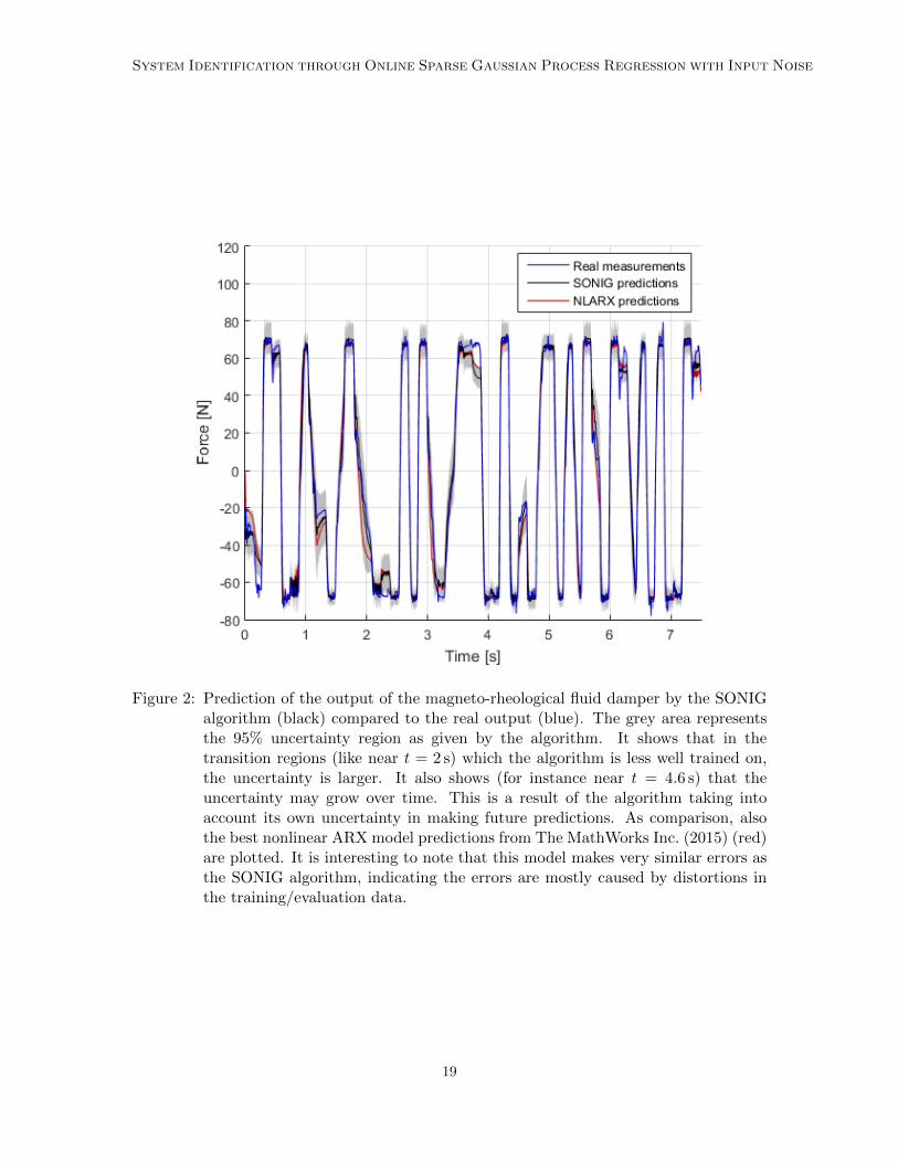
After all training measurements had been used, the SONIG algorithm was given theinput data for the remaining 1499 measurements, but not the output data. It had topredict this output data by itself, using each prediction yk to predict the subsequent yk+1.While doing so, the algorithm also calculated the variance of each prediction yk, taking thisinto account while predicting the next output using the techniques from Section 4.5. Theresulting predictions can be seen in Figure 2.

A comparison of the algorithm with various other methods is shown in Table 2. We alsoadded in regular GP regression and NIGP, applied to the ARX model (1), as comparison.This table shows that the SONIG algorithm, when applied in its system identification set-up, can clearly outperform other black-box modeling approaches. It is better than regularGP regression at taking into account uncertainties and better than NIGP mainly due tothe reasons explained before. It should be noted here, however, that this is all subject tothe proper tuning of hyperparameters and the proper choice of inducing input points. Withdifferent hyperparameters or inducing input point selection strategies, the performance ofthe SONIG algorithm will degrade slightly, though it is still likely to outperform otheridentification algorithms.

6. Conclusions and recommendations

We can conclude that the presented SONIG algorithm works as intended. Just like the FITCalgorithm that it expands upon, it is mainly effective when there are more measurementsthan the NIGP algorithm (or regular GP regression) can handle. The SONIG algorithmcan then include the additional measurements very efficiently—incorporating each trainingpoint in constant runtime—resulting in a higher accuracy than what the NIGP algorithmcould have achieved. However, even when this is not the case, the SONIG algorithm hason average a better performance than the NIGP algorithm, though it still needs the NIGPalgorithm for hyperparameter tuning.

18


Figure 2: Prediction of the output of the magneto-rheological fluid damper by the SONIGalgorithm (black) compared to the real output (blue). The grey area representsthe 95% uncertainty region as given by the algorithm. It shows that in thetransition regions (like near t = 2 s) which the algorithm is less well trained on,the uncertainty is larger. It also shows (for instance near t = 4.6 s) that theuncertainty may grow over time. This is a result of the algorithm taking intoaccount its own uncertainty in making future predictions. As comparison, alsothe best nonlinear ARX model predictions from The MathWorks Inc. (2015) (red)are plotted. It is interesting to note that this model makes very similar errors asthe SONIG algorithm, indicating the errors are mostly caused by distortions inthe training/evaluation data.

19

Bijl

Table 2: Comparison of various system identification models and algorithms when appliedto data from the magneto-rheological fluid damper. All algorithms were given2000 measurements for training and 1499 measurements for evaluation.

Algorithm RMSE Source

Linear OE model (4th order) 27.1 The MathWorks Inc. (2015)

Hammerstein-Wiener (4th order) 27.0 The MathWorks Inc. (2015)

NLARX (3rd order, wavelet network) 24.5 The MathWorks Inc. (2015)

NLARX (3rd order, tree partition) 19.3 The MathWorks Inc. (2015)

NIGP 10.2 This paper

GP regression 9.87 This paper

NLARX (3rd order, sigmoid network) 8.24 The MathWorks Inc. (2015)

RR GP-SSM 8.17 Svensson et al. (2016)

SONIG 7.12 This paper

Though the SONIG algorithm can be used for any type of regression problem, it hasbeen successfully applied, in its system identification set-up, to a nonlinear black-box systemidentification problem. With the proper choice of hyperparameters and inducing inputpoints, it outperformed existing state-of-the-art nonlinear system identification algorithms.

Nevertheless, there are still many improvements that can be made to the SONIG algo-rithm. For instance, to improve the accuracy of the algorithm, we can look at reducing someof the approximating assumptions, like the linearization assumption (13) or the assumptionthat higher order terms of Σ+ are negligible.

Another way to improve the accuracy of the algorithm is to increase the number ofinducing input points, but this will slow down the algorithm. To compensate, we couldlook into updating only the few nearest inducing input points (with the highest covariance)when incorporating a new training point. Experience has shown that updates hardly affectinducing inputs far away from the training point (with a low covariance) so this could leadto more efficient updates.

A final possible improvement would concern the addition of a smoothing step in thealgorithm. Currently, early measurements are used to provide more accuracy for latermeasurements, but not vice versa. If we also walk back through the measurements, like ina smoothing algorithm, a higher accuracy might be obtained.

Acknowledgments

This research is supported by the Dutch Technology Foundation STW, which is part of theNetherlands Organisation for Scientific Research (NWO), and which is partly funded bythe Ministry of Economic Affairs. The work was also supported by the Swedish researchCouncil (VR) via the projects NewLEADS - New Directions in Learning Dynamical Systemsand Probabilistic modeling of dynamical systems (Contract number: 621-2016-06079, 621-2013-5524) and by the Swedish Foundation for Strategic Research (SSF) via the project

20


ASSEMBLE (Contract number: RIT15-0012). We would also like to thank Marc Deisenrothfor fruitful discussion and in particular for pointing us to the NIGP algorithm.

Appendix. Derivatives of prediction matrices

The SONIG update law (16) contains various derivatives of matrices. Using (8) and (9) wecan find them. To do so, we first define the scalar quantity

P = Σn++ + σ2n = K++ + σ2n −K+uK

−1uu (Kuu − Σn

uu)K−1uuKu+. (27)

We also assume that m(x) = 0 for ease of notation. (If not, this can of course be taken intoaccount.) The derivatives of µn+1

u and Σn+1uu can now be found element-wise through

dµn+1u

dx+j

= ΣnuuK

−1uu

(dKu+

dx+j

P−1(y+ −K+uK

−1uuµ

nu

)+Ku+

dP−1

dx+j

(y+ −K+uK

−1uuµ

nu

)− Ku+P

−1dK+u

dx+j

K−1uuµ

nu

),

d2µn+1u

dx+jdx+k

= ΣnuuK

−1uu

(d2Ku+

dx+jdx+k

P−1(y+ −K+uK

−1uuµ

nu

)+dKu+

dx+j

dP−1

dx+k

(y+ −K+uK

−1uuµ

nu

)−dKu+

dx+j

P−1dK+u

dx+k

K−1uuµ

nu +

dKu+

dx+k

dP−1

dx+j

(y+ −K+uK

−1uuµ

nu

)+Ku+

d2P−1

dx+jdx+k

(y+ −K+uK

−1uuµ

nu

)−Ku+

dP−1

dx+j

dK+u

dx+k

K−1uuµ

nu

−dKu+

dx+k

P−1dK+u

dx+j

K−1uuµ

nu −Ku+

dP−1

dx+k

dK+u

dx+j

K−1uuµ

nu −Ku+P

−1 d2K+u

dx+jdx+k

K−1uuµ

nu

),

dΣn+1uu

dx+j

= −ΣnuuK

−1uu

(dKu+

dx+j

P−1K+u +Ku+dP−1

dx+j

K+u +Ku+P−1dK+u

dx+j

)K−1

uu Σnuu,

d2Σn+1uu

dx+jdx+k

= −ΣnuuK

−1uu

(d2Ku+

dx+jdx+k

P−1K+u +dKu+

dx+j

dP−1

dx+k

K+u +dKu+

dx+j

P−1dK+u

dx+k

+dKu+

dx+k

dP−1

dx+j

K+u +Ku+d2P−1

dx+jdx+k

K+u +Ku+dP−1

dx+j

dK+u

dx+k

+dKu+

dx+k

P−1dK+u

dx+j

+Ku+dP−1

dx+k

dK+u

dx+j

+Ku+P−1 d2K+u

dx+jdx+k

)K−1

uu Σnuu. (28)

These expressions contain various additional derivatives. To find them, we need to choosea covariance function. (The above expressions are valid for any covariance function.) If we

21

Bijl

use the squared exponential covariance function of (4), we can derive

dKui+

dx+= α2 exp

(−1

2(xui − x+)T Λ−1 (xui − x+)

)(xui − x+)T Λ−1,

d2Kui+

dx2+

= α2 exp

(−1

2(xui − x+)T Λ−1 (xui − x+)

)(Λ−1 (xui − x+) (xui − x+)T Λ−1 − Λ−1

),

dP−1

dx+= −P−2 dP

dx+= 2P−2

(K+uK

−1uu (Kuu − Σn

uu)K−1uu

dKu+

dx+

),

d2P−1

dx2+

=d

dx+

(−P−2 dP

dx+

)= 2P−3

(dP

dx+

)T ( dP

dx+

)− P−2 d

2P

dx2+

,

dP

dx+= −2K+uK

−1uu (Kuu − Σn

uu)K−1uu

dKu+

dx+,

d2P

dx2+

= −2dK+u

dx+K−1

uu (Kuu − Σnuu)K−1

uu

dKu+

dx+− 2K+uK

−1uu (Kuu − Σn

uu)K−1uu

d2Ku+

dx2+

. (29)

References

Mauricio A. Alvarez, Lorenzo Rosasco, and Neil D. Lawrence. Kernels for vector-valuedfunctions: A review. Foundations and Trends in Machine Learning, 4(3):195–266, 2012.

Hildo Bijl. SONIG source code, 2017. URL https://github.com/HildoBijl/SONIG/tree/v1.0.

Hildo Bijl, Jan-Willem van Wingerden, Thomas B. Schon, and Michel Verhaegen. Onlinesparse Gaussian process regression using FITC and PITC approximations. In Proceedingsof the IFAC symposium on System Identification, SYSID, Beijing, China, October 2015.

Joaquin Q. Candela and Carl E. Rasmussen. A unifying view of sparse approximate Gaus-sian process regression. Journal of Machine Learning Research, 6:1939–1959, 2005.

Joaquin Q. Candela, Agathe Girard, Jan Larsen, and Carl E. Rasmussen. Propagation ofuncertainty in Bayesian kernel models - application to multiple-step ahead forecasting.In Advances in Neural Information Processing Systems, pages 701–704. MIT Press, 2003.

Krzysztof Chalupka, Christopher K. I. Williams, and Iain Murray. A framework for evaluat-ing approximation methods for Gaussian process regression. Machine Learning Research,14:333–350, 2013.

Tianshi Chen, Henrik Ohlsson, and Lennart Ljung. On the estimation of transfer functions,regularizations and Gaussian processes–revisited. Automatica, 48(8):1525–1535, 2012.

Legel Csato and Manfred Opper. Sparse online Gaussian processes. Neural Computation,14(3):641–669, 2002.

Patrick Dallaire, Camille Besse, and Brahim Chaib-draa. Learning Gaussian process modelsfrom uncertain data. In Proceedings of the 16th International Conference on NeuralInformation Processing, December 2009.

22


Andreas C. Damianou, Michalis K. Titsias, and Neil D. Lawrence. Variational inference forlatent variables and uncertain inputs in Gaussian processes. Journal of Machine LearningResearch, 17(42), 2016.

Marc P. Deisenroth. Efficient Reinforcement Learning using Gaussian Processes. PhDthesis, Karlsruhe Institute of Technology, 2010.

Marc P. Deisenroth and Jun W. Ng. Distributed Gaussian processes. In Proceedings of theInternational Conference on Machine Learning (ICML), Lille, France, 2015.

Marc P. Deisenroth and Carl E. Rasmussen. PILCO: A model-based and data-efficientapproach to policy search. In Proceedings of the International Conference on MachineLearning (ICML), Bellevue, Washington, USA, pages 465–472. ACM Press, 2011.

Roger Frigola, Fredrik Lindsten, Thomas B. Schon, and Carl E. Rasmussen. Bayesianinference and learning in Gaussian process state-space models with particle MCMC. InAdvances in Neural Information Processing Systems (NIPS) 26, Lake Tahoe, NV, USA,December 2013.

Roger Frigola, Yutian Chen, and Carl E. Rasmussen. Variational Gaussian process state-space models. In Advances in Neural Information Processing Systems (NIPS), 2014.

Yarin Gal, Mark van der Wilk, and Carl E. Rasmussen. Distributed variational inferencein sparse Gaussian process regression and latent variable models. In Advances in NeuralInformation Processing Systems (NIPS), 2014.

Agathe Girard and Roderick Murray-Smith. Learning a Gaussian process model with un-certain inputs. Technical Report 144, Department of Computing Science, University ofGlasgow, June 2003.

Agathe Girard, Carl E. Rasmussen, Joaquin Q. Candela, and Roderick Murray-Smith.Gaussian process priors with uncertain inputs - application to multiple-step ahead timeseries forecasting. In Advances in Neural Information Processing Systems, pages 529–536.MIT Press, 2003.

Paul W. Goldberg, Christopher K. I. Williams, and Christopher M. Bishop. Regression withinput-dependent noise: A Gaussian process treatment. In Advances in Neural InformationProcessing Systems (NIPS), volume 10, pages 493–499. MIT Press, January 1997.

James Hensman, Fusi Nicolo, and Neil D. Lawrence. Gaussian processes for big data.In Proceedings of the Twenty-Ninth Conference on Uncertainty in Artificial Intelligence(UAI), Bellevue, Washington, USA, 2013.

Marco F. Huber. Recursive Gaussian process regression. In Proceedings of the IEEE Inter-national Conference on Acoustics, Speech and Signal Processing (ICASSP), Vancouver,Canada, pages 3362–3366, May 2013.

Marco F. Huber. Recursive Gaussian process: On-line regression and learning. PatternRecognition Letters, 45:85–91, 2014.

23

Bijl

Jus Kocijan. Modelling and control of dynamic systems using Gaussian process models.Springer, Basel, Switzerland, 2016.

Jus Kocijan, Agathe Girard, Blaz Banko, and Roderick Murray-Smith. Dynamic systemsidentification with Gaussian processes. Mathematical and Computer Modelling of Dy-namical Systems, 11(4):411—424, 2005.

Peng Kou, Feng Gao, and Xiaohong Guan. Sparse online warped Gaussian process for windpower probabilistic forecasting. Applied Energy, 108:410–428, August 2013.

Quoc V. Le and Alex J. Smola. Heteroscedastic Gaussian process regression. In Proceedingsof the International Conference on Machine Learning (ICML), Bonn, Germany, 2005.

Lennart Ljung. System Identification: Theory for the User. Prentice Hall, Upper SaddleRiver, NJ, USA, 1999.

Andrew McHutchon. Nonlinear Modelling and Control using Gaussian Processes. PhDthesis, Churchill College, August 2014.

Andrew McHutchon and Carl E. Rasmussen. Gaussian process training with input noise.In Advances in Neural Information Processing Systems (NIPS), Granada, Spain, pages1341–1349, December 2011.

Gianluigi Pillonetto and Giuseppe De Nicolao. A new kernel-based approach for linearsystem identification. Automatica, 46(1):81—93, 2010.

Gianluigi Pillonetto, Alessandro Chiuso, and Giuseppe De Nicolao. Prediction error iden-tification of linear systems: a nonparametric Gaussian regression approach. Automatica,47(2):291—305, 2011.

Ananth Ranganathan, Ming-Hsuan Yang, and Jeffrey Ho. Online sparse Gaussian processregression and its applications. IEEE Transactions on Image, 20(2):391–404, 2011.

Carl E. Rasmussen and Christopher K.I. Williams. Gaussian Processes for Machine Learn-ing. MIT Press, 2006.

Matthias Seeger, Christopher K.I. Williams, and Neil D. Lawrence. Fast forward selectionto speed up sparse Gaussian process regression. In Proceedings of the Ninth InternationalWorkshop on Artificial Intelligence and Statistics (AISTATS), Key West, FL, USA, Jan-uary 2003.

Alex J. Smola and Peter Bartlett. Sparse greedy Gaussian process regression. In Advancesin Neural Information Processing Systems (NIPS), Vancouver, Canada, pages 619–625,2001.

Edward Snelson and Zoubin Ghahramani. Variable noise and dimensionality reduction forsparse Gaussian processes. In Proceedings of the Twenty-Second Conference on Uncer-tainty in Artificial Intelligence (UAI), Cambridge, Massachusetts, USA, 2006a.

Edward Snelson and Zoubin Ghahramani. Sparse Gaussian processes using pseudo-inputs.In Advances in Neural Information Processing Systems (NIPS), pages 1257–1264, 2006b.

24


Andreas Svensson and Thomas B. Schon. A flexible state space model for learning nonlineardynamical systems. Automatica, 80:189–199, June 2017.

Andreas Svensson, Arno Solin, Simo Sarkka, and Thomas B. Schon. Computationallyefficient Bayesian learning of Gaussian process state space models. In Proceedings of the19th International Conference on Artificial Intelligence and Statistics (AISTATS), Cadiz,Spain, May 2016.

The MathWorks Inc. Nonlinear modeling of a magneto-rheological fluid damper. Exam-ple file provided by Matlab R© R2015b System Identification ToolboxTM, 2015. Avail-able at http://mathworks.com/help/ident/examples/nonlinear-modeling-of-a-magneto-rheological-fluid-damper.html.

Michalis K. Titsias. Variational learning of inducing variables in sparse Gaussian processes.In Proceedings of the International Conference on Artificial Intelligence and Statistics(AISTATS), Clearwater Beach, FL, USA, 2009.

Michalis K. Titsias and Neil D. Lawrence. Bayesian Gaussian process latent variable model.In Proceedings of the Thirteenth International Conference on Artificial Intelligence andStatistics (AISTATS 13), pages 844–851, 2010.

Chunyi Wang and Radford M. Neal. Gaussian process regression with heteroscedastic ornon-Gaussian residuals. Technical report, arXiv.org, 2012.

Jiandong Wang, Akira Sano, Tongwen Chen, and Biao Huang. Identification of Hammer-stein systems without explicit parameterization of nonlinearity. International Journal ofControl, 82(5):937–952, 2009.

25

System Identi cation through Online Sparse Gaussian Process Regression with...

Documents

Transcript of System Identi cation through Online Sparse Gaussian Process Regression with...