Synthetic or Real?

The Equilibrium Effects of Credit Default Swaps

on Bond Markets ∗

Martin Oehmke †

Columbia University

Adam Zawadowski ‡

Boston University

June 29, 2014

Abstract

We provide a model of non-redundant credit default swaps (CDSs), building on the observation

that CDSs are more liquid than bonds. CDS introduction involves a trade-off: It crowds out demand

for the bond, but improves the bond allocation because it allows long-term investors to become levered

basis traders. CDS introduction raises bond prices only when there is a significant liquidity difference

between bond and CDS (both across and within firms). Our framework predicts a negative CDS-bond

basis, turnover and price impact patterns that are consistent with empirical evidence, and shows that

a ban on naked CDSs can raise borrowing costs.

∗For helpful comments and suggestions, we thank Jennie Bai, Snehal Banerjee, Patrick Bolton, Willie Fuchs, HaitaoLi, Xuewen Liu, Konstantin Milbradt, Uday Rajan, Suresh Sundaresan, Dimitri Vayanos, and Haoxiang Zhu, as well asconference and seminar participants at the 2013 Red Rock Conference, 2014 AFA Annual Meeting (Philadelphia), BostonUniversity, Brandeis University, BIS, Vienna GSF, Singapore Management University, Nanyang Technological University,National University of Singapore, HKUST, Humboldt Universitat zu Berlin, Columbia University, Michigan State University,Wharton, the Boston Fed, the 2014 SFS Calvacade, LSE, and the 2014 WFA.†Columbia Business School, 420 Uris Hall, 3022 Broadway, New York, NY 10027, e-mail: moehmke@columbia.edu,

http://www0.gsb.columbia.edu/faculty/moehmke‡Boston University School of Management, 595 Commonwealth Avenue, Boston, MA 02215, e-mail: zawa@bu.edu, http:

//www.people.bu.edu/zawa

1 Introduction

Credit Default Swap (CDS) markets have grown enormously over the last decade. However, while

there is a relatively large literature on the pricing of CDSs, much less work has been done on the

economic role of these markets. For example, in most pricing models, CDSs are redundant securities,

such that the introduction of a CDS market has no effect on the underlying bond market. This

irrelevancy feature makes a meaningful analysis of the economic role of CDS markets difficult.

In this paper, we develop a theory of non-redundant CDS markets, building on a simple, well-

documented empirical observation: Trading bonds is expensive relative to trading CDSs. Based on

this observation, we develop a theory of the interaction of bond and CDS markets and the economic

role of CDSs. Our model provides an integrated framework that matches many of the stylized facts

in bond and CDS markets: the effect of CDS markets on the price of the underlying bond (and

therefore financing cost for issuers), the relative pricing of the CDS and the underlying bond (the

CDS-bond basis), and trading volume in the bond and CDS markets. Our model also provides a

tractable framework to assess policy interventions in CDS markets, such as the recent E.U. ban of

naked CDS positions.

In our model, investors differ across two dimensions. First, investors differ in their investment

horizons: Some investors are unlikely to have to sell their position in the future and are therefore similar

to buy-and-hold investors, such as insurance companies. Other investors are more likely to receive

liquidity shocks and therefore have shorter investment horizons. These investors can be interpreted

as active traders, such as speculators or hedge funds. Second, investors have heterogeneous beliefs

about the bond’s default probability: Optimistic investors view the default of the bond as unlikely,

while pessimists think that a default is relatively more likely. If only the bond is traded, relatively

optimistic investors with sufficiently long trading horizons buy the bond, whereas relatively pessimistic

investors with sufficiently long trading horizons take short positions in the bond. Investors with short

1

investment horizons stay out of the market, because for them the transaction costs of trading the

bond are too high.

The introduction of a CDS affects the underlying bond market through three effects: (1) Some

investors who previously held a long position in the bond switch to selling CDS protection, putting

downward pressure on the bond price. (2) Investors who previously shorted the bond switch to buying

CDS protection because, in equilibrium, the relatively illiquid bond trades at a discount compared

to the CDS. The resulting reduction in short selling puts upward pressure on the bond price. (3)

Some investors become “negative basis traders” who hold a long position in the bond and purchase

CDS protection (i.e., the model endogenously generates the negative basis trade, which has been an

immensely popular trading strategy in recent years). If basis traders cannot take leverage, they do

not affect the price of the underlying bond. If basis traders can take leverage—a natural assumption

given that they hold hedged positions—they push up the bond price. In practice, basis trades are

often highly levered and their leverage varies with financial conditions, leading to time-series variation

in the strength of this third effect.

Taken together, these three effects imply that, in general, CDS introduction is associated with an

ambiguous change in the price of the underlying bond. This prediction is consistent with the empirical

literature, which has found no unconditional effect of CDS introduction on bond or loan spreads (Hirtle

(2009), Ashcraft and Santos (2009)). More importantly, our model identifies the underlying economic

trade-off that determines the effect of CDS introduction. One the one hand, CDS introduction can

crowd out demand for the bond, while on the other hand it leads to an allocational improvement in

the bond market, because the presence of the CDS allows long-term investors to hold more of the

bond supply. The balance of this trade-off critically depends on the relative liquidity of the bond

and the CDS: When the bond and the CDS are similar in terms of their liquidity, the crowding

out effect dominates and CDS introduction lowers bond prices. On the other hand, when there is a

substantial difference in the liquidity of the CDS and the underlying bond, the introduction of the

CDS tends to raise bond prices. The same logic implies that, for firms with multiple bond issues of

2

differing liquidity (e.g., “on-the-run” and “off-the-run” bonds), illiquid bonds benefit relatively more

from CDS introduction. In fact, the price effect of CDS introduction can go in opposite directions for

bonds of differing liquidity issued by the same company; the price of the illiquid bond increases while

the price of the liquid bond decreases.

The endogenous emergence of leveraged basis traders highlights a novel economic role of CDS

markets: The introduction of a relatively more liquid derivative market allows buy-and-hold investors,

who are efficient holders of the illiquid bond, to hedge undesired credit risk in the more liquid CDS

market. In the CDS market, the average seller of CDS protection is relatively optimistic about the

bond’s default probability, but is not an efficient holder of the bond because of more frequent liquidity

shocks. The role of CDS markets is thus similar to liquidity transformation—by repackaging the

bond’s default risk into a more liquid security, they allow the transfer of credit risk from efficient

holders of the bond to relatively more optimistic shorter-term investors, such as hedge funds. Hence,

when bonds are illiquid, a liquid CDS can improve the allocation of credit risk and thus presents an

alternative to recent proposals that aim at making the corporate bond market more liquid, for example

through standardization.1 This liquidity view of CDS markets differs from the traditional view that

the main function of CDSs is simply the separation of credit risk and interest rate risk.2 However,

because the separation of interest rate risk from credit risk is also possible via a simple interest rate

swap, it is unlikely that this traditional view captures the full economic role of CDS markets.

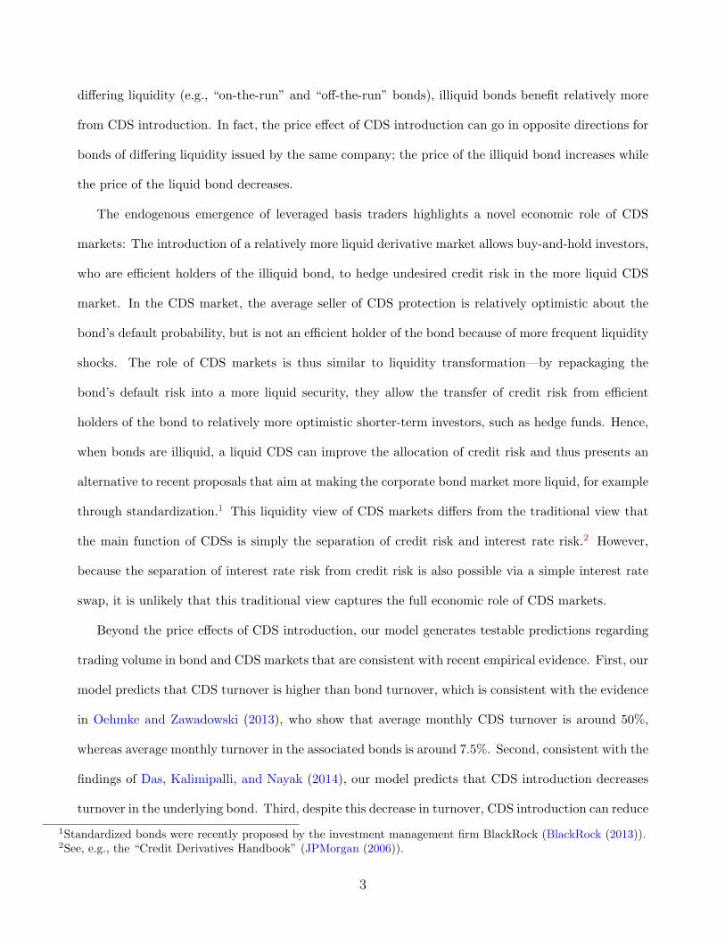
Beyond the price effects of CDS introduction, our model generates testable predictions regarding

trading volume in bond and CDS markets that are consistent with recent empirical evidence. First, our

model predicts that CDS turnover is higher than bond turnover, which is consistent with the evidence

in Oehmke and Zawadowski (2013), who show that average monthly CDS turnover is around 50%,

whereas average monthly turnover in the associated bonds is around 7.5%. Second, consistent with the

findings of Das, Kalimipalli, and Nayak (2014), our model predicts that CDS introduction decreases

turnover in the underlying bond. Third, despite this decrease in turnover, CDS introduction can reduce

1Standardized bonds were recently proposed by the investment management firm BlackRock (BlackRock (2013)).2See, e.g., the “Credit Derivatives Handbook” (JPMorgan (2006)).

3

price impact in the bond market, such that, consistent with Das, Kalimipalli, and Nayak (2014), the

effect of CDS introduction on bond market liquidity can differ depending on which particular illiquidity

measure is used.

From an asset pricing perspective, the prediction that the equilibrium price of the bond is (weakly)

less than the price of a synthetic bond consisting of a risk-free bond and a short position in the CDS

replicates a well-documented empirical phenomenon known as the negative CDS-bond basis (see,

e.g., Bai and Collin-Dufresne (2010) and Fontana (2011)). Here our model generates a number of

predictions regarding both the time-series and cross-sectional variation in the CDS-bond basis: The

basis is more negative if the bond is more illiquid, when there is more disagreement about the bond’s

default probability, and when basis traders are restricted in the amount of leverage they can take.

Finally, our model provides a framework to study regulatory interventions with respect to CDS

markets. For example, a ban on naked CDS positions, as recently imposed by the European Union on

sovereign bonds through EU regulation 236/2012, may, in fact, raise yields for affected issuers. This

can happen because, if pessimistic investors cannot take naked CDS positions, some of them will short

the bond instead. This exerts downward price pressure on bond prices: Due to the liquidity difference

between bonds and CDSs, naked CDS positions and short bond positions are not equivalent because

a different set of investors takes the other side.3

Our paper contributes to a growing literature on derivatives as non-redundant securities.4 In our

framework, the source of non-redundancy is a difference in the market liquidity of the underlying

security and the derivative, which we model using the classic framework of Amihud and Mendelson

(1986). Given the well-documented illiquidity of corporate bonds, we view liquidity as a source of non-

redundancy to be particularly important in the context of the CDS market. Other contributions to

this literature have focused on different (and potentially complementary) sources of non-redundancy,

3In addition to the naked CDS ban, we also briefly explore the effects of banning CDS markets altogether and banningboth CDS markets and short positions in the underlying bond. In general, also these interventions have ambiguous effectson bond yields.

4Hakansson (1979) provides an early discussion of why derivatives should be studied in settings where they are notredundant.

4

including market incompleteness (Detemple and Selden (1991)), the informational effects of derivative

markets (Grossman (1988), Biais and Hillion (1994), Easley, O’Hara, and Srinivas (1998), and Gold-

stein, Li, and Yang (2014)), the possibility that derivatives generate sunspots (Bowman and Faust

(1997)), and changes in the relative bargaining power of debtors and creditors (Bolton and Oehmke

(2011), Arping (2014)).

In addition, a number of recent papers have investigated the role of derivatives in the presence of

short-sale and collateral constraints. Banerjee and Graveline (2014) show that derivatives can relax

binding short-sales constraints when the underlying security is scarce (i.e., on “special”). Fostel and

Geanakoplos (2012) show that, in the presence of collateral constraints in the spirit of Geanakoplos

(2010) and Simsek (2013), the introduction of CDSs can lead to financial busts because they allow

pessimistic investors to bet more effectively against the underlying asset. Che and Sethi (2013) show

that naked CDSs facilitate leveraged negative bets that can increase a firm’s cost of capital. In

contrast to these papers, our approach does not rely on explicit short-sale or collateral constraints (or

their relaxation). This means, for example, that our framework applies also in situations where the

underlying asset can be shorted relatively easily.5 Garleanu and Pedersen (2011) explore the relative

pricing of derivatives and underlying assets when derivatives have lower margin requirements and apply

this framework to the CDS-bond basis. Shen, Yan, and Zhang (2013) develop a model of financial

innovation based on differences in collateral requirements. However, these papers do not focus on the

consequences of derivative introduction on the underlying asset, which is the main focus of our paper.

While, leaning on empirical evidence, we take the difference in market liquidity between the CDS

and the underlying bond as given, a number of search-theoretic models have explored endogenous

differences in liquidity between assets with identical payoffs (Vayanos and Wang (2007), Vayanos and

Weill (2008), Weill (2008)). In this context, Praz (2013) studies the interaction between a (liquid)

5In contrast to some markets where short selling is indeed difficult to impossible, this feature of our model may be relevantwhen it comes to corporate bond markets: Asquith, Au, Covert, and Pathak (2013) document that shorting costs in thecorporate bond market are modest on average and comparable to those in the stock market.

5

Walrasian and a (less liquid) OTC market, while Sambalaibat (2013) studies the effect of naked CDS

trading in search markets.

More generally, our paper contributes to a growing literature on the economic effects of CDS mar-

kets. Duffee and Zhou (2001), Morrison (2005), Parlour and Plantin (2008), Parlour and Winton

(2013), and Thompson (2009) explore how CDS markets allow banks to lay off credit risk and affect

funding and monitoring outcomes. Allen and Carletti (2006) investigate how the availability of CDSs

affects financial stability. Yorulmazer (2013) develops a model of CDSs as a means of regulatory arbi-

trage. Zawadowski (2013) develops a model in which CDSs are used to hedge counterparty exposures

in a financial network. Atkeson, Eisfeldt, and Weill (2012) provide a model of the market structure of

CDS and other OTC derivative markets. Overviews of CDS markets and current policy debates can

be found in Stulz (2010), Jarrow (2011), and Bolton and Oehmke (2013).6

2 Model Setup

We consider a financial market with (up to) two assets: (i) a defaultable bond and (ii) a CDS that

references the bond. The main assumption of our model is that the bond and the CDS, which offer

exposure to the same credit risk, differ in liquidity. This difference in liquidity makes the CDS non-

redundant.7

Illiquidity and high transaction costs in the corporate bond market have been widely documented.8

In contrast, CDS markets tend to be relatively liquid. In fact, it has become standard in the asset

6There is also a growing empirical literature on price discovery in CDS markets (Acharya and Johnson (2007), Hilscher,Pollet, and Wilson (2014)), the effect of CDSs on leverage and maturity (Saretto and Tookes (2013)), the determinants ofCDS market existence and CDS positions (Oehmke and Zawadowski (2013)), the CDS-bond basis (Blanco, Brennan, andMarsh (2005), Bai and Collin-Dufresne (2010), Fontana (2011), Li, Kim, and Zhang (2010)).

7This liquidity view of CDS markets echoes Ashcraft and Santos (2009) who, in their empirical study of the effects ofCDS introduction, point out that “Liquidity in the bond market has been limited because many investors hold their bondsuntil maturity. The secondary market for loans has experienced rapid growth in the recent years, but bank loans remainlargely illiquid. Under these circumstances, the development of the CDS market provided banks and investors with a new,less expensive, way to hedge or lay off their risk exposures to firms.”

8See, e.g., Bessembinder, Maxwell, and Venkataraman (2006), Edwards, Harris, and Piwowar (2007), Mahanti, Nashikkar,Subrahmanyam, Chacko, and Mallik (2008), Bao, Pan, and Wang (2011). Effective trading costs for bonds include bothbid-ask spreads and the market impact of trading and are usually much larger than quoted bid-ask spreads. In a samplethat contains the most liquid bonds in the TRACE database, Bao, Pan, and Wang (2011) estimate effective trading costs forcorporate bonds to be between 74 and 221 basis points, depending on the size of the trade. Transactions costs for less liquid

6

pricing literature to assume that the CDS market is perfectly liquid (see Longstaff, Mithal, and Neis

(2005)).9 Following Amihud and Mendelson (1986), we model illiquidity by assuming that investors

incur trading costs, which we interpret broadly as reflecting both bid-ask spreads and market impact

costs. Our main assumption, based on the evidence discussed above, is that these trading costs are

lower for the CDS than the associated bond.

While we take the difference in liquidity between the bond market and the CDS market as given,

a number of factors contribute to the relative liquidity of CDS markets when compared to bonds or

loans. The first is standardization: The bonds issued by a particular firm are usually fragmented into a

number of different issues which differ in their coupons, maturities, covenants, embedded options, and

other features. The resulting fragmentation reduces the liquidity of these bonds. The CDS market, on

the other hand, provides a standardized venue for the firm’s credit risk (for a more detailed description

see Stulz (2010)). Consistent with this argument, Oehmke and Zawadowski (2013) show that, CDS

markets are more active and more likely to exist for firms whose outstanding bonds are fragmented into

many separate bond issues. Second, a CDS investor who has to terminate an existing CDS position

prior to maturity rarely sells his CDS in the secondary market; rather than selling the original contract

he simply enters an offsetting CDS contract, which is usually cheaper. Third, inventory management

for market makers is generally cheaper for CDS dealers than for market makers in bond markets.

bonds are even higher. Very large trades ($10M+) are hard to execute in the bond market and usually have large transactioncosts (Randall (2013)). CDS trades, on the other hand, are routinely at least $10M, which is the typical unit of trade.

9While this assumption is not literally true, traders and other market participants generally view the CDS market as moreliquid than the market for the underlying bonds. Unfortunately, transaction data to calculate the effective trading costs ofCDSs is not available. However, a rough comparison of CDS and bond trading costs can be obtained by comparing CDSbid-ask spreads to effective bond trading costs. For CDSs, the bid-ask spread should capture most of the effective tradingcosts: Because CDS spreads are generally quoted for large trade sizes, market impact is less important for CDS trading coststhan for bond trading costs. To compare CDS bid-ask spreads to bond trading costs, the CDS bid-ask spread has to bemultiplied by the tenor (maturity) of the CDS. In fact, this approach likely overstates effective CDS roundtrip costs, becauseinvestors typically shop around for the best bid and ask prices, such that the roundtrip cost is the inside bid-ask spread(lowest ask minus highest bid) instead of the average bid-ask spread which is typically reported. Hilscher, Pollet, and Wilson(2014) report bid-ask spreads of 4-6 basis points for five-year credit default swaps on IG bonds, which thus implies tradingcosts of around 20-30 basis points, significantly lower than the implied spreads reported by Bao, Pan, and Wang (2011).In fact, often the liquidity advantage of CDSs can be seen by simply comparing bid-ask spreads. For example, even in thesample of sovereign bonds (which are usually relatively liquid) in Sambalaibat (2013), 75% of the CDSs have lower bid-askspreads than the associated bonds. Finally, the liquidity advantage of CDS markets is also reflected by the fact that CDSmarkets incorporate information before bond markets (see Blanco, Brennan, and Marsh (2005) and Acharya and Johnson(2007)).

7

Because the CDS is a derivative, no ex-ante inventory has to be held. Moreover, regulatory capital

charges for inventory are often larger for bonds than for derivatives.

2.1 Bond

A defaultable bond is traded in positive supply S > 0. We denote the bond’s equilibrium ask price

by p. The bond matures with Poisson arrival rate λ. As will become clear below, the assumption

of Poisson maturity is convenient because is guarantees stationarity. However, none of our results

depend on this assumption.10 For simplicity we assume that the bond does not pay coupons.11 At

maturity, the bond pays back its face value of $1 with probability 1−π. With probability π, the bond

defaults and pays 0.12

We capture illiquidity of the bond market in terms of a bond trading cost cB that arises when the

bond is traded. Specifically, following Amihud and Mendelson (1986), we assume that the bond can

be bought at the ask price p and sold (or short sold) at the bid price p− cB. As discussed above, we

interpret these trading costs broadly as reflecting both the relatively large bid-ask spreads for bonds

and the market impact of executing the bond trade. Beyond the trading cost cB we do not impose any

additional cost on short selling. While it would be straightforward to add this to the model, treating

long and short positions symmetrically highlights that, in contrast to a number of existing paper on

CDS or derivative introduction (Banerjee and Graveline (2014), Che and Sethi (2013), Fostel and

Geanakoplos (2012)), our results do not require short-sale restrictions.13

10For other papers that use Poisson maturity as a tool to guarantee stationarity, see He and Xiong (2012) and Chen, Cui,He, and Milbradt (2013).

11It would be straightforward to allow for coupons. We omit them because the presence of coupons does not affect any ofour results and therefore merely adds notation.

12This implies that default only occurs at maturity. Alternatively, one could assume that default can occur continuouslywith Poisson arrival rate. We chose the setup with default only at maturity because it is particularly tractable and yieldsthe same economic insights as a model with continuous default.

13In fact, the evidence in Asquith, Au, Covert, and Pathak (2013) suggests that on average shorting corporate bond is notsignificantly more costly than shorting stocks, which makes a framework that does not explicitly rely on significant shortingcosts appealing.

8

2.2 Credit default swap

In addition to the bond, a CDS that references the bond is available in zero net supply. The CDS is

an insurance contract on the bond’s default risk: It pays off $1 if the bond defaults at maturity and

zero otherwise.14 For simplicity we assume that the CDS matures at the same time as the bond. We

denote the CDS’s equilibrium ask price by q.15

The (relatively low) trading cost in the CDS market is denoted by cCDS. Hence, an investors can

purchase CDS protection at the ask price q and sell protection at the bid q − cCDS. Trading costs in

the CDS market are lower than in the bond market, such that

cB ≥ cCDS ≥ 0. (1)

For most of our analysis, we follow Longstaff, Mithal, and Neis (2005) in assuming, for simplicity, that

the CDS market involves no transaction costs, such that cCDS = 0. In Section 4.4, we then extend our

analysis to the case in which cCDS > 0

2.3 Investors

There is a mass of risk-neutral, competitive investors who can trade the bond and the CDS. For

simplicity, we set the investors’ rate of time preference to zero. Investors are heterogeneous across two

dimensions: (i) expected holding periods and (ii) beliefs about default probabilities.16

14Hence, the CDS pays off an amount that is exactly equal to the loss given default of $1. We therefore abstract awayfrom potential discrepancies between the CDS payoff and the loss given default that can arise as part of the CDS settlementauction (see Chernov, Gorbenko, and Makarov (2013), Du and Zhu (2013), and Gupta and Sundaram (2013)).

15In practice, CDS contracts have fixed maturities (also known as tenors), the most common being 1, 5 and 10 years. Oursetup, where both the bond and the CDS randomly mature at the same time is comparable to a setup in which investorsmatch maturities of finite-maturity bonds and CDSs. Moreover, CDS premia are usually paid over time (quarterly), with apotential upfront payment at inception of the contract. The CDS price q should thus be interpreted as the present value offuture CDS premia and the upfront payment.

16This assumption captures that both a security’s default risk and its transaction costs matter for investors, and thatthe degree two which they matter differs across investors. As we will see below, both dimensions of heterogeneity play animportant role in our analysis.

9

Expected holding periods differ across investors because investors are hit by liquidity shocks with

Poisson intensity µi ∈ [0,∞]. Investors with low µi can be interpreted as buy-and-hold investors (for

example, insurance companies or pension funds), whereas investors with high µi are investors subject

to more frequent liquidity shocks (for example, hedge funds or other investors that are expressing

shorter-term views). When hit by a liquidity shock, an investor has to liquidate his position exits the

model. To preserve stationarity, we assume that a new investor with the same characteristics enters.

With respect to investor beliefs, we assume that investors agree to disagree about the bond’s default

probability in the sense of Aumann (1976). Specifically, investor i believes that the bond defaults at

maturity with probability πi ∈ [π − ∆2 , π + ∆

2 ]. These differences in subjective default probabilities

among investors lead to differences in valuation of the bond’s cash flows, thereby generating a motive to

trade. More generally, these differences in valuation of the bond could also be generated by differences

in investors’ non-traded endowment risks, which would result in risk-based (rather than beliefs-based)

private valuations of the bond.17

We assume that investors are uniformly distributed on the plane spanned by π and µ, with a mass

one of investors at each liquidity shock intensity µi. This assumption implies a particularly simple

density function f(µ, π) = 1∆ , which allows us to calculate equilibrium prices in closed form.

Investors can take positions in the bond (the “real” asset) and the CDS (the synthetic asset), but

are subject to portfolio restrictions that reflect risk management constraints.18 Specifically, we assume

that each investor can hold up to one unit of credit risk. Accordingly, each investor can either go long

one bond, short one bond, buy one CDS, or sell one CDS. In addition, investors can enter hedged

portfolios. One such option is to take a long position in the bond and insure it by also purchasing a

CDS (a so-called negative basis trade). Alternatively, investors can take a hedge position by taking

a short position in the bond and selling CDS protection (a so-called positive basis trade). Because

hedged positions do not involve credit risk, we allow investors to lever up hedged positions up to

17The differences-in-beliefs setup we use in our model implies that investors do not learn from prices. For a model thatstudies the informational consequences of derivatives such as CDSs see Goldstein, Li, and Yang (2014).

18Given risk neutrality and differences in beliefs among investors, absent portfolio restrictions investors would take infinitepositions.

10

a maximum leverage of L ≥ 1. Hence, L = 1 implies that hedged investors cannot take leverage,

whereas L > 1 implies that hedged investors can lever up their positions. Finally, as an outside option

investors can always hold cash, which yields a zero return.

3 Benchmark: No CDS Market

In this Section, we first briefly consider the benchmark case in which only the bond trades. Building

on this benchmark, we then turn to joint equilibrium in bond and CDS markets and the effects of

CDS introduction in Section 4.

Investors maximize their utility subject to their portfolio constraints. When only the bond is

trading, this means that investors choose between a long or a short position in the bond and holding

cash. Investor i’s net payoff from a long position in the bond is given by

VlongBOND,i = −p+µi

µi + λ(p− cB) +

λ

µi + λ(1− πi). (2)

The interpretation of this expression is as follows. The investor pays the ask price p to purchase the

bond. With probability µiµi+λ

the investor has to sell the bond before maturity. Here, the stationarity

property of Poisson maturity implies that a non-matured bond at some future liquidation date t trades

at the same price p as the bond today. Hence, the investor receives the bid price p− cB when he has

to sell the bond before maturity. If the bond matures before the investor receives a liquidity shock,

the investor receives an expected payoff of 1−πi, where πi is the investor’s subjective belief about the

bond’s default probability. This happens with probability λµi+λ

.

Similarly, investor i’s net payoff from a short position in the bond is given by

VshortBOND,i = p− cB −µi

µi + λp− λ

µi + λ(1− πi). (3)

11

An investor who takes a short position in the bond receives the bid price p− cB today. If the investor

has to cover his short position before maturity, the investor has to purchase the bond at the ask price

p (again using the stationarity property), whereas if the bond matures the investor has to cover his

short position at an expected cost of 1− πi. The probabilities of these two events are µiµi+λ

and λµi+λ

,

respectively.

Figure 1 illustrates the resulting demand for long and short positions.19 Investors that are opti-

mistic about the bonds’ default probability and have sufficiently long trading horizons purchase the

bond, forming a triangle of buyers. On the boundary of the “buy” triangle, investors are indifferent

between a long position in the bond on holing cash, which requires that VlongBOND,i = 0. Similarly,

pessimistic investors with sufficiently long trading horizons short the bond, with the boundary of the

resulting “short” triangle defined by VshortBOND,i = 0. All other investors simply hold cash. The gap

between the triangle of long bondholders and short sellers arises because the bond trading cost cB

drives a wedge between the payoffs from long and short positions, which makes it optimal even for

some investors who do not face liquidity shocks to stay out of the market.

Market clearing requires that the bond price p adjusts such that the overall amount bought by long

investors is equal to the amount shorted plus bond supply S. Solving this market clearing condition

for the bond price p leads to the following Lemma.

Lemma 1. Benchmark: Bond market equilibrium in absence of CDS market. When only

the bond trades, the equilibrium bond price is given by

pnoCDS = 1− π +cB2− cBλ

∆

∆− cBS. (4)

Lemma 1 shows that, in the absence of the CDS, the bond price is given by the average investor’s

belief about the bond’s expected payoff, 1 − π, plus two additional terms that capture the effect of

the bond’s trading costs and supply. The term cB2 captures the wedge that the bond trading cost puts

19We focus on the case in which, in the absence of the CDS, both long and short investors are present. This is the case aslong as the bond supply S is not too large. The exact condition is given in the appendix.

12

buy  

1− p

short  

€

π

( )⎟⎠

⎞⎜⎝

⎛ +−−Δ

+ BB

12

cpc

πλ

€

π −Δ2

λcB

1− p− π −Δ2

#

$%

&

'(

#

$%

&

'(

€

0

€

µ

€

π

€

π +Δ2

1− p+ cB

Figure 1: Bond market equilibrium in the absence of a CDS.

The figure illustrates the equilibrium when only the bond is trading. Investors who are sufficientlyoptimistic about the bond’s default probability and have sufficiently long holding horizons form a “buy”triangle. Investors who are pessimistic about the bond’s default probability and have sufficiently longholding horizons form a “shorting” triangle. Market clearing requires that the bond price adjust suchthat demand from long investors is equal to bond supply plus short positions.

between the payoff from a long and a short position, which increases the bond’s ask price by exactly

half of the bond’s trading cost. The term − cBλ

∆∆−cBS captures that, as the bond supply S increases,

the marginal bond investor becomes less optimistic and has shorter trading horizons, leading to a

decrease in the bond price. Note that unless the bond supply is very small, the bond trades at a

discount to its expected payoff under the average default probability. For the remainder of the paper

we will assume that this condition holds, such that pnoCDS < 1 − π. More formally, this assumption

can be stated as:

Assumption 1. The bond supply satisfies S > λ2

∆−cB∆ .

13

4 Introducing a CDS Market

We now introduce the CDS contract to the analysis. Analogously to before, we determine the demand

for the CDS by calculating the payoffs from positions that involve the CDS: long and short CDS

positions as well as hedged positions in the bond and the CDS. Combining these payoffs with the

payoffs to going long or short in the bond, derived in equations (2) and (3), we then solve for joint

equilibrium in the bond and the CDS market.

The net payoff to investor i of purchasing a CDS on the bond is given by

VbuyCDS,i = −q +µi

µi + λ(q − cCDS) +

λ

µi + λπi. (5)

This expression reflects the purchase price q of the CDS, the payoff q − cCDS from early liquidation

at the bid with probability µiµi+λ

(using stationarity) and the expected CDS payoff of πi in the case

of default at maturity, which happens with probability λµi+λ

. Analogously, the payoff to investor i of

selling a CDS on the bond is given by

VsellCDS,i = q − cCDS −µi

µi + λq − λ

µi + λπi. (6)

In addition to taking directional positions in the bond or the CDS, investors can enter hedged “basis

trade” positions. Because hedged positions can be levered L times, these hedged portfolios pay off

L · (VbuyCDS,i + VlongBOND,i) in the case of a negative basis trade and L · (VsellCDS,i + VshortBOND,i) for

a positive basis trade. Finally, investors can still hold cash as an outside option with zero return.

Solving for equilibrium in the bond and CDS market requires calculating the demand for bond and

CDS positions from the above payoffs and then imposing market clearing to determine the equilibrium

prices of the bond and the CDS. In our main analysis, we will focus on the case in which the CDS

market is frictionless (cCDS = 0). After establishing our main results in the context of this particularly

14

tractable case, we discuss the case where also the CDS market is subject to trading frictions (cCDS > 0)

in Section 4.4.

4.1 The effect of CDS introduction on prices and trading in the bond market

The advantage of assuming that CDS markets are frictionless is that the equilibrium in the CDS

market becomes particularly simple: When cCDS = 0, equations (5) and (6) imply that all investors

with beliefs πi < q are willing to sell CDS protection, while all investors with πi > q are willing to

purchase CDS protection. Given that above any level of µ there is an infinite mass of agents willing

to buy and sell CDS protection, this implies that the equilibrium price of the CDS must be equal to

the average investor belief about the bond’s default probability,20

q = π. (7)

To determine the equilibrium bond price, it therefore suffices to investigate how the availability of the

CDS priced at q = π affects investors’ incentives to take long or short positions in the bond.

Consider first the case in which basis traders cannot take leverage (L = 1), depicted in Figure 2.

The figure shows that the introduction of the CDS has three effects on the equilibrium in the bond

market. First, when the CDS is available, investors with relatively short trading horizons who in

absence of the CDS used to purchase the bond now prefer to sell CDS protection. This can be seen

in Figure 2 by observing that the triangle of long bondholders has been cut off at the top (for ease of

comparison, the triangle of long bond positions in the absence of the CDS is depicted by the dashed

line). This crowding out of long bond investors leads to a reduction in demand for the bond, exerting

downward pressure on the bond price.

Second, the introduction of the CDS eliminates short selling in the bond. In the figure, the triangle

of investors that formerly shorted the bond (depicted by the dotted line on the right) vanishes, because

20Strictly speaking, we are making a limit argument: Consider and upper bound µ for the frequency of the liquidity shockand take the limit µ→∞. As the mass of traders in the CDS market grows, the CDS price q converges to π.

15

buy  bond  

1− p

€

π

λcB

1− p− q( )

sell  CDS  

buy  CDS  

λcB

1− p− π −Δ2

#

$%

&

'(

#

$%

&

'( €

µ

€

π = q

basis  

€

π +Δ2

€

π −Δ2

€

0

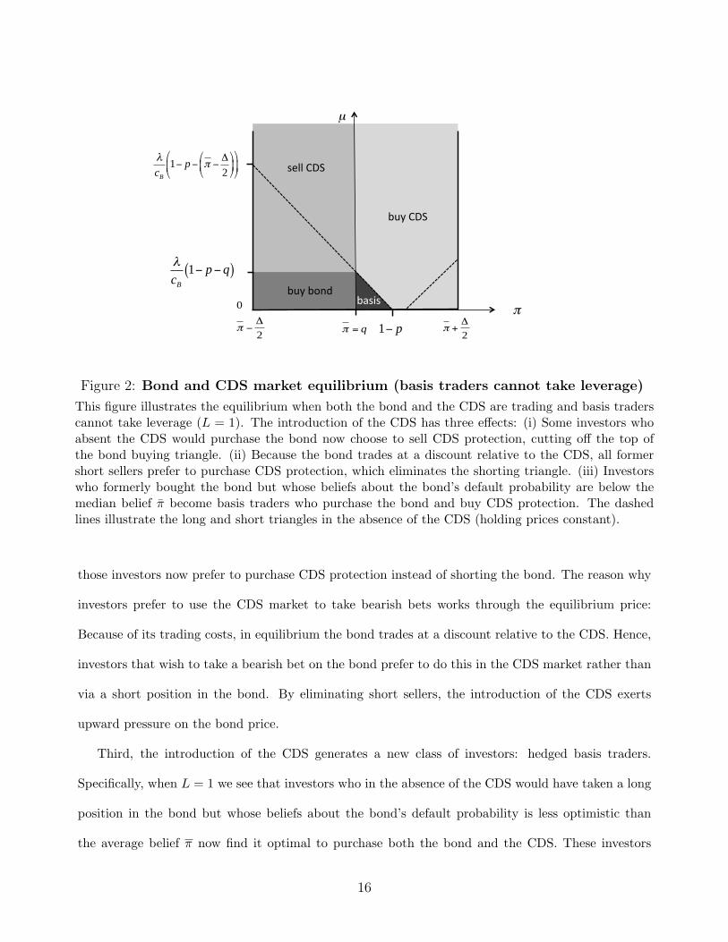
Figure 2: Bond and CDS market equilibrium (basis traders cannot take leverage)

This figure illustrates the equilibrium when both the bond and the CDS are trading and basis traderscannot take leverage (L = 1). The introduction of the CDS has three effects: (i) Some investors whoabsent the CDS would purchase the bond now choose to sell CDS protection, cutting off the top ofthe bond buying triangle. (ii) Because the bond trades at a discount relative to the CDS, all formershort sellers prefer to purchase CDS protection, which eliminates the shorting triangle. (iii) Investorswho formerly bought the bond but whose beliefs about the bond’s default probability are below themedian belief π become basis traders who purchase the bond and buy CDS protection. The dashedlines illustrate the long and short triangles in the absence of the CDS (holding prices constant).

those investors now prefer to purchase CDS protection instead of shorting the bond. The reason why

investors prefer to use the CDS market to take bearish bets works through the equilibrium price:

Because of its trading costs, in equilibrium the bond trades at a discount relative to the CDS. Hence,

investors that wish to take a bearish bet on the bond prefer to do this in the CDS market rather than

via a short position in the bond. By eliminating short sellers, the introduction of the CDS exerts

upward pressure on the bond price.

Third, the introduction of the CDS generates a new class of investors: hedged basis traders.

Specifically, when L = 1 we see that investors who in the absence of the CDS would have taken a long

position in the bond but whose beliefs about the bond’s default probability is less optimistic than

the average belief π now find it optimal to purchase both the bond and the CDS. These investors

16

thus become negative basis traders: They hold a hedged position in the bond and the CDS, thereby

locking in the equilibrium price differential between the underlying bond and the derivative. Rather

than taking bets on credit risk, these investors act as arbitrageurs.

When basis traders cannot take leverage (L = 1), as assumed in Figure 2, their presence does not

affect the bond price. The reason is that the investors in the basis trade triangle would have purchased

the bond anyway, even in absence of the CDS. When basis traders can take leverage (L > 1), on the

other hand, the ability to hedge with the CDS allows basis traders to demand more of the bond, such

that they exert upward pressure on the bond price. This is illustrated in Figure 3. More specifically,

the figure shows that the ability of basis traders to take leverage raises the equilibrium bond price in

two ways. First, holding constant the number of basis traders (i.e., keeping the size of the basis trader

triangle as in Figure 2), the ability to take leverage increases the demand for the bond from this given

set of basis traders, thereby putting upward pressure on the bond price. Second, the ability to take

leverage makes the basis trade more profitable and thereby increases the number of basis traders: As

illustrated in Figure 3, the basis trader triangle expands. In fact, when basis traders can take leverage,

even some investors to the left of π become basis traders. Even though for these investors the CDS

priced at q = π has a negative payoff when seen in isolation, they purchase the CDS because it allows

them to lever up their position in the bond.21

The emergence of basis traders highlights a novel economic role of CDS markets in our model: The

CDS improves the allocation in the bond market by allowing buy-and-hold investors to purchase more

of the bond, thereby allowing efficient holders of the illiquid bond to hold a larger share of the bond

supply. This is possible because the liquid CDS allows buy-and-hold investors to lay off the credit risk

to investors with shorter trading horizons in the CDS market. By allowing to lay off credit risk to

investors with shorter trading horizons the CDS therefore essentially serves as a vehicle for liquidity

transformation. Note that this liquidity-based view of CDSs goes beyond the traditional view that

21When the basis trade becomes extremely profitable, it is possible that the basis trade region extends all the way to theπi = π+∆/2. While this would not affect our results, we rule out this case for simplicity. The exact condition, which requiresthat bond supply or basis trader leverage are not too large, is given in the appendix.

17

buy  bond  

€

π

λcB

1− p− q( )

sell  CDS   buy  CDS  

q− (L −1) ⋅ 1− p− q( ) q+ L ⋅ 1− p− q( )

€

µ

basis  

€

π +Δ2

€

π −Δ2

€

0

€

π = q

Figure 3: Bond and CDS market equilibrium (basis traders can take leverage)

The figure illustrates the equilibrium when both the bond and the CDS are trading and basis traderscan take leverage (L > 1). The ability to take leverage makes the basis trade more attractive, suchthat the basis trade triangle expands compared to Figure 2. Because of the increased demand frombasis traders, more of the bond can be held by investors with long trading horizons, improving theallocation in the bond market. compared to the case when L = 1. For ease of comparison, the dashedline illustrates the rectangle of investors who purchase the bond when basis traders cannot take leverage(L = 1).

CDSs simply allow separate interest rate risk from default risk. In fact, separation of credit risk from

interest rate risk is possible with an interest rate swap and does not require a CDS. In contrast, the

allocational improvement through basis traders that is highlighted here is only possible via a (liquid)

CDS contract.

Given the discussion above, we now solve for the equilibrium bond price. Market clearing in

the bond market requires that the demand from investors with a long position in the bond and the

demand from basis traders add up to the bond supply S. Solving for the bond price p that satisfies

this condition yields the following Lemma.

18

Lemma 2. Bond price in presence of frictionless CDS market. When both the bond and a

frictionless CDS are traded, the CDS price is given by q = π and the equilibrium bond price is equal

to

pwithCDS = 1− π − ∆

2

√1 + 8Φ cB

λS∆ − 1

Φ, (8)

where we define Φ ≡ 1 + 2L(L− 1).

Similar to Lemma 1, the bond price in the presence of the CDS is equal to the average expected

payoff 1− π, plus an adjustment for the bond’s trading cost and bond supply. Note however that in

the presence of the CDS, this supply adjustment depends on the amount of leverage that basis traders

can take. In addition, the ability to (synthetically) short the bond via the CDS without incurring a

trading cost eliminates the wedge between long and short positions and therefore the cB2 term that

was present when no CDS is available.

Based on Lemmas 1 and 2, we are now in a position to characterize the effect of CDS introduction

on the price of the underlying bond.

Proposition 1. The effect of CDS introduction on the bond price. The change in the bond

price due to CDS introduction is given by

pwithCDS − pnoCDS = −cB2

+cBλ

∆

∆− cBS − ∆

2

√1 + 8Φ cB

λS∆ − 1

Φ. (9)

The price effect of CDS introduction on the underlying CDS is ambiguous. CDS introduction is more

likely to raise the bond price when

(i) basis trader leverage L is high,

(ii) disagreement about the default probability ∆ is low, and

(iii) the bond trading cost cB is high.

Equation (9) summarizes the effect of CDS introduction on the price of the underlying bond.

First, setting cB = 0, note that the CDS is redundant when the bond is perfectly liquid and pwithCDS−

19

pnoCDS = 0. In this case, the CDS has no liquidity advantage over the bond and therefore does not

affect the pricing of the bond. As we show in Section 4.4, this generalizes to the case in which both

the bond and the CDS have trading costs: The CDS is redundant whenever trading costs in the CDS

market are equal to trading costs in the bond market.22

Second, for the CDS to increase the bond price, the liquidity difference between the bond and

the CDS must be sufficiently large. Specifically, when the bond trading cost cB is sufficiently small,

the introduction of the CDS reduces the bond price. This can be seen by differentiating equation (9)

with respect to the bond trading cost and evaluating the resulting expression at cB = 0, which yields

−12 −

Sλ < 0. Hence, given that the price change at cB = 0 is zero, for bond trading costs close enough

to zero CDS introduction reduces the bond price. The reason is that when the bond and the CDS

are sufficiently similar in liquidity, the crowding out effect of the CDS dominates, such that the bond

price drops when the CDS is introduced.23

When cB is sufficiently large, on the other hand, CDS introduction can increase the bond price.

However, for CDS introduction to increase the bond price it has to be the case that basis traders can

take sufficient leverage: When L = 1 such that basis traders cannot take leverage, the crowding out

effect of the CDS market dominates and the bond price decreases when the CDS introduced. When L

is sufficiently large, on the other hand, the introduction of the CDS increases the bond price because

a larger share of the bond supply is absorbed by buy-and-hold investors that are less likely to incur

the trading costs of the bond. When basis traders do not face any leverage constraints (L→∞), the

bond price is given by the bond’s average expected payoff 1−π. Under Assumption 1, the bond price

therefore increases in response to CDS introduction when basis trader leverage L is sufficiently high.

Corollary 1. CDS introduction raises the bond price when basis traders can take sufficient leverage.

22More generally, in our model the CDS is redundant whenever trading costs in the CDS market are weakly larger thantrading costs in the bond market: When CDS trading costs exceed bond trading costs, investors do not take positions in theCDS market because, intuitively speaking, the bond market dominates the CDS market. Hence, CDS markets that are lessliquid than the bond require additional frictions, such as restrictions on short selling.

23While in Proposition 1 we keep the CDS trading cost cCDS fixed at 0 and vary the bond trading cost cB we show inSection 4.4 that this insight carries over to the setting where both the bond and the CDS are subject to strictly positivetrading costs.

20

The comparative statics with respect to cB and L highlight the main economic trade-off that arises

when the CDS is introduced. On one hand, CDS introduction crowds out demand for the bond

which puts downward pressure on the equilibrium bond price. On the other hand, CDS introduction

improves the allocation in the bond market because it allows investors with long horizons to hold more

off the illiquid bond, which puts upward pressure on the equilibrium bond price. As shown above,

when the liquidity differential between the bond and the CDS is sufficiently large and when basis

traders can take sufficient leverage, the second effect dominates and the bond price increases when

the CDS is introduced. While we have focused on the uniform investor distribution in characterizing

the trade-off between the crowding out effect and the allocational improvement that is possible in the

presence of the CDS, the underlying economic insight is not distribution-specific. What is distribution

specific, is the result that CDS introduction always reduces the bond price when L = 1 (i.e., that the

crowding out of long bond positions outweighs the reduction in short selling).24

Finally, Proposition 1 shows that CDS introduction is less likely to increase the bond price when

disagreement about the bond’s default probability ∆ is substantial. The intuition for this finding

is as follows. Absent the CDS, the bond price is increasing in disagreement. As can be seen from

Figure 1, an increase in ∆ increases the area of the “buy” triangle more than the area of the “short”

triangle, resulting in an increase in the bond price. This reverses once the CDS is available: After

CDS introduction the bond price is decreasing in disagreement about the bond’s default probability,

which can be seen by inspecting Figure 2. An increase in ∆ leaves the mass of investors in the “buy

bond” rectangle unchanged, but drains investor mass out of the “basis” triangle, thereby leading to a

decrease in the bond price.25

24There are alternative distributions for which the reduction in short selling outweighs the crowding out of long positions,such that CDS introduction raises the bond price even for L = 1. Relative to the uniform distribution, these distributionshave a larger mass of traders with infrequent liquidity shocks (i.e., there are relatively more buy-and-hold investors), suchthat there is a larger mass of investors in the shorting triangle that is eliminated by CDS introduction (low µ) than in thetriangle of long bondholders that are crowded out by the CDS market (higher µ). See Figure 2.

25Note that, even when the CDS is available, we have continued to assume that investors need to liquidate their positionswhen hit by a liquidity shock. One could enrich the framework by assuming that sometimes it suffices that long bondinvestors hedge their bond position with a CDS when hit by a shock. This reduces the effective expected bond trading costsand therefore introduces an additional positive effect of CDS markets on bond markets: investors are more likely to purchase

21

The main empirical prediction of Proposition 1 is that the price effect of CDS introduction on

bond prices is generally ambiguous and depends crucially on bond and firm characteristics. This

is consistent with an emerging empirical literature on the effect of CDSs on the cost of financing for

firms. Ashcraft and Santos (2009) find no evidence that the introduction of CDS contracts has lowered

financing costs for the average borrower, but document modest reductions in spreads for safe firms.

Hirtle (2009) finds only limited evidence that CDSs have improved firms’ access to financing, with

positive effects of CDSs on access to credit concentrated among larger term borrowers. Moreover,

the specific empirical patterns regarding which types of borrowers benefit from CDS introduction

are in line with the predictions of our model. Consistent with the prediction that CDS introduction

is less likely to increase bond prices when there is substantial disagreement, Ashcraft and Santos

(2009) find that firms with high earnings forecast dispersion face increased funding costs once a CDS

is introduced. Ashcraft and Santos (2009), Nashikkar, Subrahmanyam, and Mahanti (2011), and

Shim and Zhu (2014) show evidence consistent with the prediction that bond and CDS must differ

sufficiently in liquidity for CDSs to reduce funding costs. Because we have set cCDS = 0, the relative

liquidity difference in our benchmark model is captured simply by the bond trading cost cB. In Section

4.4 we extend our model to allow for positive CDS trading costs cCDS > 0 and provide a more detailed

discussion of the role of the relative liquidity of the bond and the CDS and the associated empirical

evidence there.

In addition to the result on the effects of CDS introduction on the bond price, our model generates

implications for turnover in the bond and the CDS market. First, our model predicts that CDS

introduction reduces turnover in the bond market (defined as bond trading volume divided by the

supply of the bond S). This can be seen directly from Figure 2. As a result of CDS introduction,

bond investors with relatively short trading horizons switch to selling the CDS, thereby reducing

bond turnover. In addition, the introduction of the CDS eliminates short sellers, which also leads to

a reduction in bond turnover. Second, our model predicts that when both the bond and the CDS are

the bond because sometimes they can use the CDS to hedge ex post. However, subject to this adjustment, all other effectsdescribed above would remain at work.

22

available, turnover in the CDS market (defined as the amount of CDS trading divided by the notional

amount of outstanding CDSs) exceeds turnover in the bond market. This implication follows from

a clientele effect a la Amihud and Mendelson (1986), whereby investors with higher average trading

frequencies hold the CDS whereas investors who trade less hold the bond.26

However, while CDS introduction reduces turnover in the bond market, this does not imply that

the bond market becomes less liquid when looking at price impact. Specifically, when basis traders can

take sufficient leverage, the sensitivity of the bond price with respect to a supply shock, | dpdS |, is smaller

when a CDS is available. Hence, while the allocational changes that results from the introduction of

the CDS reduce bond turnover, the fact that basis traders stand ready to absorb supply shocks reduces

price impact in the bond market. Accordingly, the effect of CDS introduction on bond liquidity may

differ depending on which liquidity measure (e.g., turnover or price impact) is used. We summarize

these results in the following proposition.

Proposition 2. Turnover and price impact in bond and CDS markets.

(i) Turnover in the CDS market is higher than turnover in the bond market.

(ii) Turnover in the underlying bond decreases when the CDS is introduced.

(iii) Price impact in the bond market decreases when the CDS is introduced if basis traders can take

sufficient leverage.

The first two predictions in Proposition 2 follow relatively directly from the differences in trading

costs between the bond and the CDS and the resulting clientele effect that arises as investors sort

themselves into these two assets depending on the frequency of their liquidity shocks. Nonetheless,

these additional predictions are useful because they offer additional dimensions along which we can

link our model to empirical evidence. In fact, consistent with the first prediction in Proposition

2, Oehmke and Zawadowski (2013) document that average monthly CDS turnover (based on CDS

trading data from the DTCC) is 50.8% per month, whereas average turnover in the associated bonds

26This simple comparison of average trading frequencies of investors suffices because there is no short selling when the CDStrades.

23

(as reported by TRACE) is around 7.5% per month. Consistent with the second prediction, Das,

Kalimipalli, and Nayak (2014) show that CDS introduction is indeed associated with a decrease in

turnover in the underlying bond. Hence, the observed turnover patters in bond and CDS markets

match the predictions of our model. Finally, the third prediction in Proposition 2 provides a potential

explanation of why Das, Kalimipalli, and Nayak (2014) find that the effect of CDS introduction on

bond liquidity differs depending on which specific liquidity measure is used: While our framework

predicts a reduction in bond turnover, the effect of CDS introduction on price impact depends on

model parameters, such as basis trader leverage and the outstanding supply of the underlying bond.

Consistent with this prediction, Das, Kalimipalli, and Nayak (2014) do not find a clear directional

effect when investigating the effect of CDS introduction on the Amihud price impact measure (Amihud

(2002)).

4.2 The CDS-bond basis

In this section, we investigate the relative pricing of the bond and the CDS once both instruments

trade. The relative pricing of bonds and CDSs is captured by the CDS-bond basis, which has attracted

considerable attention in the wake of the financial crisis of 2007-2009. The CDS-bond basis is defined

as the difference between the spread of a synthetic bond (composed of a long position in a risk-free

bond of the same maturity and coupon as the risky bond and a short position in the CDS) and

the spread of the actual risky bond. Intuitively speaking, when the CDS-bond basis is negative, the

bond spread is larger than the CDS spread, which means that the physical bond is cheaper than the

payoff-equivalent synthetic bond.

Absent frictions, the CDS-bond basis should be approximately zero. The reason is that a portfolio

consisting of a long bond position and a CDS that insures the default risk of the bond should yield the

risk-free rate.27 Since the financial crisis, the CDS-bond basis has been consistently negative for most

27See Duffie (1999) for conditions under which this arbitrage relationship holds exactly.

24

reference entities, as documented by Bai and Collin-Dufresne (2010), Fontana (2011) and Garleanu

and Pedersen (2011).28

In our framework, a negative basis between bonds and CDSs arises endogenously from the difference

in trading costs of the bond and the CDS. To calculate the basis, note that in our setting a risk-free

bond with the same maturity as the risky bond trades at a price of one (since there is no discounting).

We can then calculate the spread of the risky bond above the risk-free rate by calculating the price

difference between the risk-free and the risky bond and dividing it by the expected time to maturity

1/λ, which yields spreadbond = λ(1−p). Analogously, given the CDS price q we can calculate the CDS

spread (the flow cost of CDS protection) as spreadCDS = λq. Hence, the CDS-bond basis is given by

basis = spreadCDS − spreadbond = −λ (1− p− q) . (10)

Based on the bond and CDS market equilibrium derived above, the CDS-bond basis then satisfies

the following properties.

Proposition 3. The CDS-bond basis. The CDS-bond basis in the presence of frictionless CDS

markets (cCDS = 0) is given by

basis = −λ∆

2

√1 + 8Φ cB

λS∆ − 1

Φ≤ 0, (11)

where Φ ≡ 1 + 2L(L− 1). The CDS-bond basis is more negative when

(i) bond supply S is large,

(ii) basis traders can take less leverage (small L),

(iii) bond trading costs cB are high,

(iv) disagreement about the bond’s default probability ∆ is high.

28Note, however, that positive bases do occur in some cases. They are usually attributed to frictions that are outside ofour model, such as short-selling constraints that arise from imperfections in the repo market, the cheapest-to-deliver option,and control rights associated with the underlying bond (see JPMorgan (2006)).

25

The source of the negative basis in our model is straightforward. Because trading costs for the

bond are higher than those of the CDS, the bond trades at a discount relative to the CDS. This

prediction is in line with a growing empirical literature that documents a negative CDS-bond basis.

In addition, Proposition 3 makes a number of time-series and cross-sectional predictions on the CDS-

bond basis. First, the basis becomes more negative in response to supply shocks in the bond market.

Such supply shocks may capture situations in which investors subject to regulatory constraints are

forced to sell some of their holdings as documented, for example, in Ellul, Jotikasthira, and Lundblad

(2011). Second, higher basis trader leverage compresses the negative basis. This is because higher

leverage for basis traders increases the demand for the bond, pushing up the bond price and thereby

reducing the negative basis. In the time series, this implies that at times when basis traders can take

substantial leverage, the basis should be less negative and closer to zero. In contrast, during times

of tough financing conditions for basis traders, the equilibrium basis will be driven away from zero

and becomes more negative. Empirical evidence suggests that this mechanism was indeed a major

contributor to the widening of the negative basis during the financial crisis, when margins rose and

arbitrageurs had to delever (see Garleanu and Pedersen (2011), Fontana (2011), and Mitchell and

Pulvino (2012)). Choi and Shachar (2014) provide evidence that it was specifically the unwinding

of CDS-bond basis trades by arbitrageurs that was a main cause of the large negative basis in 2008.

Oehmke and Zawadowski (2013) provide evidence that basis traders became relatively more active

again when financing conditions eased in mid 2009.

The remaining two comparative statics in Proposition 3 make cross-sectional predictions on the

CDS-bond basis. First, bonds with high trading costs (relative to trading costs in the associated CDS)

are predicted to have more negative CDS-bond bases. This is consistent with the empirical evidence in

Bai and Collin-Dufresne (2010). Second, our model predicts that bonds for which investors disagree

significantly on default probabilities have more negative bases. In practice, high-yield bonds tend

to be characterized by more disagreement about default probabilities and have higher trading costs.

For both of these reasons, our model therefore predicts that lower-rated bonds should have a more

26

negative basis, which is consistent with the evidence in Bai and Collin-Dufresne (2010) and Garleanu

and Pedersen (2011).

4.3 Two bond issues

In this subsection, we extend our model to a setting where an issuer has multiple bonds outstanding: a

liquid issue and a less liquid issue. One interpretation of this setting is that the liquid issue is a recently

issued “on-the-run” bond, while the less liquid issue is an older “off-the-run” bond. Alternatively, the

liquid bond may be a relatively standard bond issue, whereas the illiquid bond represents a bond

that is more custom-tailored towards a particular clientele and therefore less liquid. Finally, based on

empirical evidence that longer-term bonds are less liquid, the illiquid bond could be interpreted as a

long-term bond.

We continue to assume that the CDS is frictionless (cCDS = 0) and is therefore more liquid than

either of the two bonds, which have strictly positive trading costs of cLB (low trading cost) for the

liquid bond and cHB > cLB (high trading cost) for the illiquid bond.29 Figure 4 illustrates the holding

regions, which can be derived in analogous fashion to the one-bond case. The figure shows that the

illiquid bond is held by investors with longer trading horizons. Moreover, in equilibrium the less liquid

bond has a larger illiquidity discount and therefore a more negative CDS-bond basis.

Because of the difference in ownership patterns for the two bonds, CDS introduction affects the

prices of the two bonds differently. The liquid bond and the CDS are relatively close substitutes (in

terms of liquidity), which means that the liquid bond is affected disproportionately by the crowding-

out effect of CDS introduction. The illiquid bond and the CDS, on the other hand, are less close

substitutes, which implies that the illiquid bond benefits disproportionately from the increased demand

from basis traders. Hence, the illiquid bond generally benefits more from CDS introduction (in a

29To reduce the number of cases discussed in this extension, we assume that cLB is not too small. This simplifies theanalysis because it ensures that absent the CDS investors do not take long-short positions (similar to on-the-run/off-the-runstrategies) in the two bonds. However, this could be incorporated without affecting the main insights of this section.

27

relative sense). Moreover, as we illustrate below, it is possible that the price effect of CDS introduction

goes in opposite directions for the liquid and the illiquid bonds.

λcB

L1− pL − q( )

buy  CDS  

€

µ

€

π

L ⋅ 1− pH − q( )+ qq− (L −1) ⋅ 1− pH − q( )

€

π +Δ2

€

π −Δ2

€

0

buy  liquid  

buy  illiquid  

λcB

H − cBL

pL − pH( )

sell  CDS  

basis  illiquid  

€

π = q

basis    liquid  

Figure 4: Bond and CDS market equilibrium with two bonds of different liquidity.

The figure illustrates the equilibrium when two bonds of different liquidity and a (more liquid) CDS aretraded. Relative to the liquid bond, the illiquid bond is held by investors and basis traders with longertrading horizons. Because the two bonds are held by different investor clienteles, they are affecteddifferently by CDS introduction. The liquid bond is disproportionately affected by the crowding outeffect of the CDS market, the illiquid bond benefits disproportionately from the emergence of basistraders. The illiquid bond therefore benefits more from CDS introduction.

Figure 5 illustrates the price effect of CDS introduction on two bonds of differing liquidity for

specific parameter values. When basis trader leverage is sufficiently small (L < L∗), CDS introduction

reduces the price of both the liquid and the illiquid bond. However, because the liquid bond is affected

more strongly by the crowding out effect of the CDS, the price of the liquid bond drops by more than

the price of the illiquid bond. For an intermediary range of basis trader leverage (L∗ < L < L∗∗), the

prices of the two bonds move in opposite directions when the CDS is introduced—the illiquid bond

benefits from CDS introduction, while the price of the liquid bond decreases. Finally, when basis

28

trader leverage is sufficiently high (L > L∗∗), the prices of both bonds increase in response to CDS

introduction, but the price of the illiquid bond increases by more then the price of the liquid bond.

illiquid bond

liquid bond

2 4 6 8 10 12 14L

-0.010

-0.005

0.005

0.010

0.015

0.020Change in bond price

L* L**

Figure 5: Price change of liquid and illiquid bond due to CDS introduction

This figure illustrate the price change for a liquid and an illiquid bond in response to CDS introduction,as a function of basis trader leverage L. For low levels of basis trader leverage, both bond prices dropin response to CDS introduction, but the price of the illiquid bond drops by less. For an intermediaryrange of basis trader leverage, the price of the illiquid bond increases but the price of the liquid bonddecreases in response to CDS introduction. When basis trader leverage is sufficiently high, both bondprices increase, but the price of the illiquid bond increases by more when the CDS is introduced.Parameters: SH = 0.2, SL = 0 cH = 0.02, cL = 0.01, π = 0.1, ∆ = 0.1, λ = 0.2. Note that the supplyof the liquid bond is set to zero simply because it allows for a particularly tractable way to solve forbond prices when two bonds are trading.

Formally, we can summarize the results on CDS introduction in the presence of two bonds in the

following proposition.

Proposition 4. The effect of CDS introduction on liquid and illiquid bonds of the same

issuer. Assume an issuer has a liquid and an illiquid bond outstanding, with trading costs cLB and

cHB > cLB , respectively. The price change from CDS introduction is larger for the illiquid bond than for

the liquid bond,

pHwithCDS − pHnoCDS > pLwithCDS − pLnoCDS. (12)

Hence, the illiquid bond is more likely to benefit from CDS introduction than the liquid bond.

29

Proposition 4 makes the empirical prediction that for firms that have multiple bond issues, the

price effects of CDS introduction should differ for bonds of differing liquidity, with more illiquid bonds

more likely to benefit from CDS introduction. Because of the relative price changes in response

to CDS introduction, the availability of a CDS may affect the types of bonds that firms issue. In

particular, because more illiquid bonds benefit disproportionately from CDS introduction, this may

lead firms to issue more of these types of bonds. For example, to the extent that liquidity arises from

custom tailoring bonds to particular investor clienteles, the presence of the CDS may allow firms to

tailor their bonds more to particular holders, such as insurance companies or pension funds, given

that the availability of the CDS allows them the take levered hedged positions. Similarly, the result

in Proposition 4 provides a potential explanation of the finding that CDS introduction is associated

with an increase in the average maturity at which firms borrow (Saretto and Tookes (2013)): Because

longer maturity bonds are typically less liquid,30 a larger positive price effect of CDS introduction on

more illiquid bonds makes issuing long-term bonds more attractive.

4.4 CDS market with frictions (cCDS > 0)

In the analysis above, we focused on the particularly tractable case in which CDSs involve no trading

costs (cCDS = 0). This assumption made solving for the equilibrium in the CDS market particularly

easy because it ensured that q = π, which allowed us to solve sequentially for equilibrium prices in the

CDS and in the bond market. When cCDS > 0, on the other hand, we can no longer solve sequentially

for the CDS price q and the bond price p. Rather, we have to solve jointly for the bond and CDS price

pair (p, q). Because now also the CDS price reflects trading frictions it is generally the case that q 6= π.

While closed-form solutions are not available for this case, in this section we demonstrate the main

economic results derived above continue to hold. An advantage of extending our model to cCDS > 0

30For empirical evidence on the positive relationship between maturity and illiquidity of corporate bonds see Longstaff,Mithal, and Neis (2005), Chen, Lesmond, and Wei (2007), Edwards, Harris, and Piwowar (2007), and Bao, Pan, and Wang(2011).

30

is that it allows us to link our findings more precisely to empirical evidence that has investigated the

role of CDS market liquidity on pricing in the bond market.

Figure 6 illustrates the effect of introducing trading costs also in the CDS market. In contrast to

the frictionless CDS case, it is no longer the case that all investors for which πi < π are willing to

sell CDS protection and that all investors with πi > π are willing to purchase CDS protection. The

“sell CDS” and “buy CDS” regions are now triangles—rather than rectangles as in Figures 2 and

3—because some investors now prefer to stay out of the market altogether and hold cash.

Despite these differences, the main qualitative results derived in the frictionless CDS setting above

remain valid. As before, the introduction of a CDS affects the bond market through three effects: (i)

the CDS crowds out some long bondholders, (ii) the CDS eliminates short sellers, and (iii) the CDS

leads to the emergence of hedged, potentially leveraged basis traders. As in the frictionless model,

basis traders are price neutral when L = 1, whereas basis traders exert upward pressure on the bond

price when they can take leverage L > 1.

Proposition 5. CDS introduction when also the CDS market is subject to trading costs.

When also the CDS market is subject to trading costs (0 < cCDS ≤ cB), then:

• the CDS is redundant when cCDS = cB,

• for cCDS sufficiently close to but less than cB, CDS introduction leads to a reduction in the bond

price,

• for CDS introduction to raise bond price, (i) there must be a sufficient difference in liquidity

between the CDS and the bond and (ii) basis traders have to be able to take sufficient leverage.

Proposition 5 highlights that the main trade-off between a crowding-out effect and an improvement

in the allocation of the bond to investors with longer holding horizons survives also in the case when

cCDS > 0: The bond market benefits from CDS introduction only if the bond and the CDS are

sufficiently different with respect to their trading costs and when basis traders can take on sufficient

leverage.

31

λcB − cCDS

1− p− q+ cCDS( )sell  CDS  

buy  CDS  

λcCDS

π +Δ2− q

#

$%

&

'(

€

µ

€

π

€

πbasis  

€

π +Δ2

€

π −Δ2

€

0

q− (L −1) ⋅ 1− p− q( )

λcCDS

q− π −Δ2

#

$%

&

'(− cCDS

#

$%

&

'(

λcB + cCDS

1− p− q( )

1− p+ (L −1) ⋅ 1− p− q( )

buy  bond  

Figure 6: Bond and CDS market equilibrium when cCDS > 0 and L > 1

The figure illustrates the equilibrium when also the CDS involves trading frictions (cCDS > 0) and basistraders can take leverage (L > 1). Compared to Figure 3 (where cCDS = 0) the “sell CDS” and “buyCDS” regions are now triangles, reflecting higher expected CDS trading costs for investors with morefrequent trading needs (higher µ). As in the case with frictionless CDS, the introduction of the CDShas three effects: (i) Some investors who absent the CDS would purchase the bond now choose to sellCDS protection, cutting of the top of the bond buying triangle. (ii) Because of the negative CDS-bondbasis, all former short sellers prefer to purchase a CDS, which eliminates the shorting triangle. (iii)Basis traders (who purchase the bond and buy CDS protection) emerge, putting upward pressure onthe bond price.

This is illustrated in the left panel of Figure 7, which plots the effect of CDS introduction on the

bond price as a function of the CDS trading cost cCDS. Each of the three lines in the plot corresponds

to different levels of basis trader leverage L. When the CDS has the same trading cost as the bond

(cCDS = 0.02), the CDS is redundant and CDS introduction has no effect on the price of the bond.31

When cCDS is slightly smaller than the bond trading cost, the crowding-out effect of the CDS dominates

and CDS introduction leads to a decrease in the bond price, independent of the amount of leverage

that basis traders can take. However, as the liquidity differential between the bond and the CDS

31More generally, the CDS is redundant in our framework whenever CDS trading costs are weakly larger than trading costsin the bond.

32

widens, basis traders emerge in equilibrium. When basis traders can take leverage (the figure depicts

L = 3 and L = 20), they improve the allocation in the bond market and put upward pressure on the

bond price. For the parameter values in this example, basis trader leverage of L = 3 is not sufficient to

generate an increase in the bond price, even as cCDS approaches 0. When L = 20, on the other hand,

CDS introduction increases the bond price when the CDS trading cost cCDS is sufficiently small. The

right panel illustrates the associated equilibrium CDS-bond basis. When calculated at ask prices,32

the CDS-bond basis is positive when cCDS is sufficiently close to cCDS. In this region, basis traders

are not active. Once cCDS is sufficiently smaller than cB, the basis becomes negative and basis traders

enter. As the Figure illustrates, the more leverage basis traders can take, the more aggressively they

lean against the negative CDS-bond basis and compress it towards zero.

The prediction that a more liquid CDS market makes it more likely that CDS introduction has a

positive effect on bond prices is indeed borne out in the data. Ashcraft and Santos (2009) show that,

while there is no reduction in funding costs for average firms in response to CDS introduction, firms

whose CDSs become liquid experience a reduction in the cost of bank loans, which, just like bonds, are

less liquid than CDS contracts.33 Nashikkar, Subrahmanyam, and Mahanti (2011) show that bonds

of firms that have more liquid CDS contracts have lower yields than those of firms for which the

associated CDS is less liquid even after controlling for bond and issuer characteristics. Finally, using

Asian CDS and bond data, Shim and Zhu (2014) find that firms with more liquid CDSs face lower

costs in primary bond markets.

Economically speaking, the prediction that sufficiently liquid CDS markets can improve the allo-

cation in the bond market provides an interesting angle on the recent discussion on standardization in

the bond market. For example, in a recent proposal, BlackRock (2013) argues for more standardized

corporate bonds in order to improve liquidity in the secondary bond market. However, as some have

argued, such standardization may come at the expense of tailoring bond issues to particular clienteles.

32We calculate the basis at ask prices because this reflects the tradeable strategy of a negative basis trader who has topurchase both the bond and the CDS at ask prices.

33Ashcraft and Santos do not find the same effect when looking at at-issue bond spreads, which they attribute to lack ofdata.

33

L=20

L=3

L=1

cCDS = cB

0.005 0.010 0.015 0.020cCDS

-0.015

-0.010

-0.005

0.005

0.010

pCDS-pno CDS

cCDS = cB

L=20

L=3

L=1

0.005 0.010 0.015 0.020cCDS

-60

-40

-20

20

40basis HbpsL

Figure 7: Price effect of CDS introduction and CDS-bond basis when cCDS > 0

The left panel shows the bond price change in response to CDS introduction as a function of the CDStrading cost cCDS. The CDS is redundant when cCDS = cB and reduces the bond price when the bondand the CDS have similar liquidity. When the CDS is sufficiently more liquid than the bond, CDSintroduction can increase the bond price if basis traders can take sufficient leverage. The right panelillustrates the CDS-bond basis. When the CDS trading cost cCDS is close to the bond trading cost cB,the basis (calculated at ask prices) is slightly positive, but no basis traders are active. When the CDSis sufficiently more liquid than the bond, the basis becomes negative and basis traders become activeand lean against the basis. Parameters: S = 0.2, cl = 0.02, π = 0.1, ∆ = 0.12, λ = 0.2, uniforminvestor distribution.

Our analysis suggests that a liquid CDS market can lead to benefits similar to those of bond stan-

dardization, while still allowing issuers to cater their bond issues to specific investor clienteles. Hence,

the introduction of a liquid zero net supply derivative can be seen as a “backdoor” way to some of the

benefits of bond standardization.

5 Policy Implications

In this section, we apply our framework to analyze a number of policy interventions in the CDS market.

Specifically, we consider the effects of (i) banning naked CDS positions (as recently implemented by

the European Union with respect to sovereign bonds), (ii) banning CDS markets altogether, and (iii)

banning both CDSs and short positions in bonds. The motivation for such interventions is usually

to achieve a reduction in bond yields (and thereby borrowing costs) for issuers. While our simple

framework is not rich enough to yield detailed policy prescriptions, it does suggest that the effects

of such interventions on bond yields can be subtle and can potentially go in the “wrong” direction

34

(i.e., contrary to the policymaker’s objective such interventions can in fact increase borrowing costs

for issuers).34

5.1 Banning naked CDS positions

EU regulation No 236/2012, in effect since November 1, 2012, bans purchasing CDS protection as a

means of speculation on sovereign bonds. Specifically, the regulation allows CDS purchases for market

participants who own the underlying bond or have other significant exposure to the sovereign, but

restrict so-called naked CDS positions. Short selling of the bond is allowed under this regulation as

long as the short seller is able to borrow the bond before executing the short sale.

The crucial question in assessing the effect of a ban on naked CDS positions is what investors who

were previously holding naked CDS protection choose to do instead. Our framework suggests that

there are three effects, which are illustrated in Figure 8: First, some of these investors switch from

a naked CDS position to a short position in the bond. Hence, as a result of a ban on naked CDSs,

short sellers reappear, putting downward pressure on the bond price. Second, some investors who

formerly held a naked CDS position become basis traders and hold the bond and the CDS, up to the

maximum leverage L. This second effect increases demand for the bond, resulting in upward pressure

on the bond price. Third, some investors that previously held naked CDS protection switch to simply

holding cash.

The effect of banning naked CDS positions on the cost of borrowing therefore depends on the

relative size of these effects and without further restrictions, can go in either direction. We illustrate

this in Figure 9: since closed form solutions are not possible, we resort to numerical solutions. The

left panel illustrates the effect of a naked CDS ban on the bond spread (solid line) and the CDS spread

(dashed line), plotted as a function of the bond trading cost cB. In this case, the naked CDS ban

generally leads to a decrease in both bond and CDS spreads. The decrease in spreads is larger, the

34While our framework allows us to investigate the positive effects of certain policy interventions, it does not allow us todetermine whether a given policy objective (such as a reduction in yields) is desirable from a normative perspective. Thisreflects the well-known difficulty of making welfare statements in models with heterogeneous beliefs.

35

sell  CDS  

€

µ

€

π

€

π

€

π +Δ2

€

π −Δ2

short  

λcCDS

q− π −Δ2

#

$%

&

'(− cCDS

#

$%

&

'(

λcB − cCDS

1− p− q+ cCDS( ) λcB

π +Δ2+ p−1− cB

#

$%

&

'(

q− (L −1) ⋅ 1− p− q( ) 1− p+ L ⋅ 1− p− q( )+ cB€

0

λcB + cCDS

1− p− q( )buy  bond  

basis  

Figure 8: Banning naked CDS when cCDS > 0 and L > 1

The figure illustrates the equilibrium when naked CDS positions are banned. Compared to Figure6, which depicts the same setup except that naked CDS positions are allowed, there are two majorchanges. Some investors who used to purchase naked CDS protection now choose to short the bond,exerting downward pressure on the bond price. Some investors who used to purchase naked CDSprotection now become basis traders, which exerts upward pressure on the bond price. The dashedline shows the position of CDS buyers and basis traders before the ban (assuming unchanged prices).

more illiquid the underlying bond, whereas the effect of the naked CDS ban are relatively small when

the bond is relatively liquid. Moreover, when the bond and the CDS are sufficiently similar in terms of

their liquidity, the naked CDS ban eliminates the CDS market altogether. The right panel illustrates

a similar example, except that the investor distribution in this example has more mass at low levels

of µi (i.e., there are more investors with longer holding horizons). In this case, the naked CDS ban

still unambiguously reduces the CDS spread, but for low levels of cB is may lead to an increase in

the bond spread, thereby raising the issuer’s financing costs. Moreover, even in the region where the

naked CDS ban reduces the bond spread, in this example the bond spread is significantly less sensitive

to the naked CDS ban than the CDS spread.

36

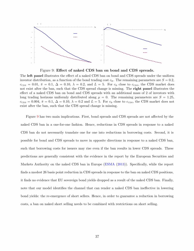
bond

CDS

0.015 0.020 0.025 0.030

cB

-35

-30

-25

-20

-15

-10

-5

spread change HbpsL

bond

CDS

0.005 0.006 0.007 0.008 0.009 0.010

cB

-12

-10

-8

-6

-4

-2

spread change HbpsL

Figure 9: Effect of naked CDS ban on bond and CDS spreads.

The left panel illustrates the effect of a naked CDS ban on bond and CDS spreads under the uniforminvestor distribution, as a function of the bond trading cost cB. The remaining parameters are S = 0.2,cCDS = 0.01, π = 0.1, ∆ = 0.10, λ = 0.2, and L = 5. For cB close to cCDS, the CDS market doesnot exist after the ban, such that the CDS spread change is missing. The right panel illustrates theeffect of a naked CDS ban on bond and CDS spreads with an additional mass of 2 of investors withlong trading horizons uniformly distributed along µ = 0. The remaining parameters are S = 1.25,cCDS = 0.004, π = 0.1, ∆ = 0.10, λ = 0.2 and L = 5. For cB close to cCDS, the CDS market does notexist after the ban, such that the CDS spread change is missing.

Figure 9 has two main implications. First, bond spreads and CDS spreads are not affected by the

naked CDS ban in a one-for-one fashion. Hence, reductions in CDS spreads in response to a naked

CDS ban do not necessarily translate one for one into reductions in borrowing costs. Second, it is

possible for bond and CDS spreads to move in opposite directions in response to a naked CDS ban,

such that borrowing costs for issuers may rise even if the ban results in lower CDS spreads. These

predictions are generally consistent with the evidence in the report by the European Securities and

Markets Authority on the naked CDS ban in Europe (ESMA (2013)). Specifically, while the report

finds a modest 26 basis point reduction in CDS spreads in response to the ban on naked CDS positions,

it finds no evidence that EU sovereign bond yields dropped as a result of the naked CDS ban. Finally,

note that our model identifies the channel that can render a naked CDS ban ineffective in lowering

bond yields: the re-emergence of short sellers. Hence, in order to guarantee a reduction in borrowing

costs, a ban on naked short selling needs to be combined with restrictions on short selling.

37

5.2 Banning the CDS market altogether

The second policy intervention we consider is an outright ban of the CDS market. This amounts to a

comparison of the equilibrium with a CDS market to the equilibrium without CDS. From Proposition

1, we know that the effect of CDS introduction on the bond yield is ambiguous. Hence, banning CDS

markets altogether may either increase or decrease borrowing costs for issuers, depending on the size

of the effects described in Sections 4.1 and 4.4. Accordingly, a ban on CDSs is more likely to lead to

a reduction in funding costs of the liquidity of the bond and the CDS market are similar and when

basis traders are restricted in the amount of leverage they can take.

5.3 Banning CDSs and short selling in the bond

Finally, we briefly consider the effect of banning both the CDS market and short positions in the

bond. This intervention amounts to a comparison of the bond and CDS market equilibrium market

described in Proposition 1 to a setting where only long positions in the bond are allowed and no CDS

is available.35 Perhaps surprisingly even this intervention is not guaranteed to lower bond yields for

issuers. While restricting short positions prevents the reemergence of short sellers in response to a ban

on CDS positions, a trade-off now emerges from the countervailing effects of (i) increased demand for

the bond from investors who formerly sold the CDS but now purchase the bond and (ii) the reduction

in demand for the bond that results from the elimination of basis traders. Because basis traders are

price neutral when they cannot take leverage (L = 1), in this case a joint ban on CDSs and short

selling leads to an unambiguous decrease in the bond yield. When basis traders can take leverage, on

the other hand, bond yields may increase or decrease, depending on the relative size of the two effects.

35This long-only case can be solved analogously to the no-CDS case in Lemma 1. The main difference is that the shortingtriangle in Figure 1 would disappear. Market clearing then requires that demand from the buying triangle equals bondsupply.

38

6 Conclusion

This paper provides a liquidity-based model of CDS markets, bond markets and their interaction. In

our framework, CDSs are non-redundant because they are more liquid than the underlying bonds. Our

model shows that the introduction of a CDS affects the underlying bond market in a non-trivial way

and identifies a fundamental trade-off between a crowding-out effect (the CDS crowds out demand for

the bond) and an improvement in the allocation in the bond market (the CDS leads to the emergence

of levered basis traders, which allows long-term investors to hold more of the illiquid bond).

CDS introduction is more likely to raise the prices of the underlying bond when there is a significant

liquidity difference between the bond and the CDS, and when hedged basis traders can take substantial

leverage. For firms with multiple bond issues, more illiquid bonds (such as off-the-run bonds or

custom-tailored issues) are more likely to benefit from CDS introduction. Beyond characterizing the

impact of CDS introduction on the pricing of the underlying bond, the model also generates empirical

predictions regarding trading volume in bond and CDS markets, as well as the cross-sectional and

time-series properties of the CDS-bond basis. It therefore provides an integrated framework that

matches many of the stylized facts in bond and CDS markets. Finally, our framework can be used

to assess a number of policy measures related to CDS markets, such as the recent E.U. ban on naked

CDS positions.

References

Acharya, V. V., and T. C. Johnson (2007): “Insider Trading in Credit Derivatives,” Journal of

Financial Economics, 84(1), 110–141.

Allen, F., and E. Carletti (2006): “Credit Risk Transfer and Contagion,” Journal of Monetary

Economics, 53, 89–111.

Amihud, Y. (2002): “Illiquidity and stock returns: cross-section and time-series effects,” Journal of

Financial Markets, 5(1), 31 – 56.

39

Amihud, Y., and H. Mendelson (1986): “Asset pricing and the bid-ask spread,” Journal of Fi-

nancial Economics, 17(2), 223–249.

Arping, S. (2014): “Credit protection and lending relationships,” Journal of Financial Stability,

10(0), 7 – 19.

Ashcraft, A. B., and J. A. C. Santos (2009): “Has the CDS Market Lowered the Cost of

Corporate Debt?,” Journal of Monetary Economics, 56(4), 514–523.

Asquith, P., A. S. Au, T. Covert, and P. A. Pathak (2013): “The market for borrowing

corporate bonds,” Journal of Financial Economics, 107(1), 155 – 182.

Atkeson, A. G., A. L. Eisfeldt, and P.-O. Weill (2012): “The Market for OTC Credit Deriva-

tives,” Working paper, UCLA.

Aumann, R. J. (1976): “Agreeing to Disagree,” Annals of Statistics, 4(6), 1236–1239.

Bai, J., and P. Collin-Dufresne (2010): “The Determinants of the CDS-Bond Basis During the

Financial Crisis of 2007-2009,” Working Paper, Swiss Finance Institute.

Banerjee, S., and J. J. Graveline (2014): “Trading in Derivatives when the Underlying is Scarce,”

Journal of Financial Economics, 111(3), 589–608.

Bao, J., J. Pan, and J. Wang (2011): “The Illiquidity of Corporate Bonds,” Journal of Finance,

66(3), 911–46.

Bessembinder, H., W. Maxwell, and K. Venkataraman (2006): “Market transparency, liq-

uidity externalities, and institutional trading costs in corporate bonds,” Journal of Financial Eco-

nomics, 82(2), 251–288.

Biais, B., and P. Hillion (1994): “Insider and liquidity trading in stock and options markets,”

Review of Financial Studies, 7(4), 743–780.

40

BlackRock (2013): “Setting New Standards: The Liquidity Challenge II,” BlackRock Investment

Institute.

Blanco, R., S. Brennan, and I. W. Marsh (2005): “An Empirical Analysis of the Dynamic

Relation between Investment-Grade Bonds and Credit Default Swaps,” The Journal of Finance,

60(5), 2255–2281.

Bolton, P., and M. Oehmke (2011): “Credit Default Swaps and the Empty Creditor Problem,”

Review of Financial Studies, 24(8), 2617–2655.

(2013): “Strategic Conduct in Credit Derivative Markets,” International Journal of Industrial

Organization, 31(5), 652–658.

Bowman, D., and J. Faust (1997): “Options, Sunspots, and the Creation of Uncertainty,” Journal

of Political Economy, 105(5), 957–975.

Che, Y.-K., and R. Sethi (2013): “Credit Market Speculation and the Cost of Capital,” AEJ:

Microeconomics, (forthcoming).

Chen, H., R. Cui, Z. He, and K. Milbradt (2013): “Quantifying Liquidity and Default Risks of

Corporate Bonds over the Business Cycle,” Working Paper, MIT Sloan.

Chen, L., D. A. Lesmond, and J. Wei (2007): “Corporate Yield Spreads and Bond Liquidity,”

The Journal of Finance, 62(1), 119–149.

Chernov, M., A. S. Gorbenko, and I. Makarov (2013): “CDS Auctions,” Review of Financial

Studies, 26(3), 768–805.

Choi, J., and O. Shachar (2014): “Did Liquidity Providers Become Liquidity Seekers? Evidence

from the CDS-Bond Basis During the 2008 Financial Crisis,” Working paper, University of Illinois

at Urbana-Champaign.

41

Das, S., M. Kalimipalli, and S. Nayak (2014): “Did CDS Trading Improve the Market for

Corporate Bonds?,” Journal of Financial Economics, 111(2), 495–525.

Detemple, J., and L. Selden (1991): “A General Equilibrium Analysis of Option and Stock Market

Interactions,” International Economic Review, 32(2), 279–303.

Du, S., and H. Zhu (2013): “Are CDS Auctions Biased and Inefficient?,” Working paper, MIT

Sloan.

Duffee, G. R., and C. Zhou (2001): “Credit derivatives in banking: Useful tools for managing

risk?,” Journal of Monetary Economics, 48(1), 25–54.

Duffie, D. (1999): “Credit Swap Valuation,” Financial Analyst Journal, 55(1), 73–87.

Easley, D., M. O’Hara, and P. Srinivas (1998): “Option Volume and Stock Prices: Evidence on

Where Informed Traders Trade,” Journal of Finance, 53(2), 431–465.

Edwards, A. K., L. E. Harris, and M. S. Piwowar (2007): “Corporate Bond Market Transaction

Costs and Transparency,” Journal of Finance, 62(3), 1421–1451.

Ellul, A., C. Jotikasthira, and C. T. Lundblad (2011): “Regulatory pressure and fire sales in

the corporate bond market,” Journal of Financial Economics, 101(3), 596–620.

ESMA (2013): “Final Report: ESMAs technical advice on the evaluation of the Regulation (EU)

236/2012 of the European Parliament and of the Council on short selling and certain aspects of

credit default swaps,” ESMA/2013/614.

Fontana, A. (2011): “The Negative CDS-bond Basis and Convergence Trading during the 2007/09

Financial Crisis,” Working Paper, Geneva Finance Research Institute.

Fostel, A., and J. Geanakoplos (2012): “Tranching, CDS, and asset prices: How financial

innovation can cause bubbles and crashes,” AEJ: Macroeconomics, 4(1), 190–225.

42

Garleanu, N., and L. H. Pedersen (2011): “Margin-based Asset Pricing and Deviations from the

Law of One Price,” Review of Financial Studies, 24(6), 1980–2022.

Geanakoplos, J. (2010): “The Leverage Cycle,” in NBER Macroeconomics Annual 2009, vol. 24,

pp. 1–65. University of Chicago Press.

Goldstein, I., Y. Li, and L. Yang (2014): “Speculation and Hedging in Segmented Markets,”

Review of Financial Studies, (forthcoming).

Grossman, S. J. (1988): “An Analysis of the Implications for Stock and Futures Price Volatility of

Program Trading and Dynamic Hedging Strategies,” Journal of Business, 61(3), 275–298.

Gupta, S., and R. K. Sundaram (2013): “CDS Auctions and Informative Biases in CDS Recovery

Rates,” Working Paper, NYU.

Hakansson, N. H. (1979): “The Fantastic World of Finance: Progress and the Free Lunch,” Journal

of Financial and Quantitative Analysis, 14(4), 717–734.

He, Z., and W. Xiong (2012): “Dynamic Debt Runs,” Review of Financial Studies, 25(6), 1799–

1843.

Hilscher, J., J. M. Pollet, and M. Wilson (2014): “Are credit default swaps a sideshow? Evi-

dence that information flows from equity to CDS markets,” Journal of Financial and Quantitative

Analysis, (forthcoming).

Hirtle, B. (2009): “Credit Derivatives and Bank Credit Supply,” Journal of Financial Intermedia-

tion, 18(2), 125–150.

Jarrow, R. A. (2011): “The Economics of Credit Default Swaps,” Annual Review of Financial

Economics, 3(2), 1–23.

JPMorgan (2006): “Credit Derivatives Handbook,” .

43

Li, H., G. H. Kim, and W. Zhang (2010): “The CDS-Bond Basis and the Cross Section of Corporate

Bond Returns,” Working Paper, University of Michigan.

Longstaff, F. A., S. Mithal, and E. Neis (2005): “Corporate Yield Spreads: Default Risk

or Liquidity? New Evidence from the Credit Default Swap Market,” Journal of Finance, 60(5),

2213–2253.

Mahanti, S., A. Nashikkar, M. Subrahmanyam, G. Chacko, and G. Mallik (2008): “Latent

liquidity: A new measure of liquidity, with an application to corporate bonds,” Journal of Financial

Economics, 88(2), 272–298.

Mitchell, M., and T. Pulvino (2012): “Arbitrage crashes and the speed of capital,” Journal of

Financial Economics, 104(3), 469 – 490.

Morrison, A. C. (2005): “Credit Derivatives, Disintermediation, and Investment Decisions,” Journal

of Business, 78(2), 621–647.

Nashikkar, A., M. G. Subrahmanyam, and S. Mahanti (2011): “Liquidity and Arbitrage in

the Market for Credit Risk,” Journal of Financial and Quantitative Analysis, 46, 627–656.

Oehmke, M., and A. Zawadowski (2013): “The Anatomy of the CDS Market,” Working Paper,

Columbia University.

Parlour, C. A., and G. Plantin (2008): “Loan Sales and Relationship Banking,” Journal of

Finance, 63(3), 1291–1314.

Parlour, C. A., and A. Winton (2013): “Laying off Credit Risk: Loan Sales versus Credit Default

Swaps,” Journal of Financial Economics, 107, 25–45.

Praz, R. (2013): “Equilibrium Asset Pricing in the Presence of Both Liquid and Illiquid Markets,”

Working Paper, Ecole Polytechnique Federale de Lausanne.

44

Randall, O. (2013): “Pricing and Liquidity in the US Corporate Bond Market,” Working paper,

Emory University.

Sambalaibat, B. (2013): “CDS and Sovereign Bond Market Liquidity,” Working Paper, Carnegie

Mellon University.

Saretto, A., and H. Tookes (2013): “Corporate Leverage, Debt Maturity and Credit Default

Swaps: The Role of Credit Supply,” Review of Financial Studies, 26(5), 1190–1247.

Shen, J., H. Yan, and J. Zhang (2013): “Collateral-Motivated Financial Innovation,” Review of

Financial Studies, (forthcoming).

Shim, I., and H. Zhu (2014): “The impact of CDS trading on the bond market: Evidence from

Asia,” Journal of Banking & Finance, 40(0), 460 – 475.

Simsek, A. (2013): “Belief Disagreements and Collateral Constraints,” Econometrica, 81(1), 1–53.

Stulz, R. M. (2010): “Credit Default Swaps and the Credit Crisis,” Journal of Economic Perspec-

tives, 24(1), 73–92.

Thompson, J. R. (2009): “Credit Risk Transfer: To Sell or to Insure,” Working Paper, University

of Waterloo.

Vayanos, D., and T. Wang (2007): “Search and endogenous concentration of liquidity in asset

markets,” Journal of Economic Theory, 136(1), 66–104.

Vayanos, D., and P.-O. Weill (2008): “A Search-Based Theory of the On-the-Run Phenomenon,”

Journal of Finance, 63(3), 1361–1398.

Weill, P.-O. (2008): “Liquidity premia in dynamic bargaining markets,” Journal of Economic

Theory, 140(1), 66–96.

45

Yorulmazer, T. (2013): “Has Financial Innovation Made the World Riskier? CDS, Regulatory

Arbitrage and Systemic Risk,” Working paper, Federal Reserve Bank of New York.

Zawadowski, A. (2013): “Entangled Financial Systems,” Review of Financial Studies, 26(1), 1291–

1323.

46

A Proofs

Proof of Lemma 1. We focus in the case in which, in the absence of the CDS, both long and short positions

in the bond emerge in equilibrium. This requires that the supply of the bond is not too large, S < 12λcB

(∆−cB)2

∆ .

Evaluating the zero valuation line of a long bond position, VlongBOND,i = 0, at µi = 0 and πi = π − ∆2 yields

a rectangular “buy” triangle with base 1 − p − (π − ∆2 ) and height λ

cB

(1− p− (π − ∆

2 )). Evaluating the zero

valuation line of a short bond position, VshortBOND,i = 0, at µi = 0 and πi = π + ∆2 yields a rectangular “buy”

triangle with base π − ∆2 − (1 − p + cB) and height λ

cB

(π − ∆

2 − (1− p+ cB)). Given the uniform investor

distribution f = 1/∆, market clearing then requires that

1

∆

[1

2

λ

cB

(1− p−

(π − ∆

2

))2

− 1

2

λ

cB

(π − ∆

2− (1− p+ cB)

)2]

= S, (A1)

which yields

pnoCDS = 1− π +cB2− cB

λ

∆

∆− cBS. (A2)

Proof of Lemma 2. Given that for any finite µ there is an infinite mass of investors willing to buy and sell

the CDS at q = π, the CDS price is pinned down at q = π irrespective of pricing in the bond markets. This

allows us to solve sequentially for prices in the CDS and the bond market. When a CDS priced at q = π

is available, solving VsellCDS,i > VlongBOND,i for µi show that any investor with µi >λcB

(1− p− q) strictly

prefers selling a CDS to taking a long position of the bond. Moreover, comparing the payoff from a negative

basis trade L · (VsellCDS,i + VshortBOND,i) to VlongBOND,i and VbuyCDS,i yields a basis trade triangle with base

(2L− 1)(1− p− q) and height λcB

(1− p− q). Note that, for simplicity, we focus on the case in which the basis

trader region is a triangle (i.e., it does not extend to πi = π + ∆2 ), which requires that S ≤ ∆λ(2L2+1)

8L2cB. This

conditions is satisfied when the bond supply S and basis trader leverage L are not too large. The opposite case

could be treated in a similar fashion, but we omit it for brevity as it does not yield any additional insights.

Market clearing in the bond market requires that the demand from long bond investors (the “buy bond

trapezoid”) and basis traders (the “basis trader triangle”) equals the supply of the bond (as discussed in the

text, buying CDS protection dominates short selling, such that no short sellers appear):

1

∆

{1

2

[q −

(π − ∆

2

)+ q − (L− 1)(1− p− q)−

(π − ∆

2

)](λ

cB(1− p− q)

)+

1

2

λ

cB(2L− 1)(1− p− q)2

}= S,(A3)

47

which yields

pwithCDS = 1− π − ∆

2

√1 + 8Φ cB

λS∆ − 1

Φ, (A4)

where we define Φ ≡ 1 + 2L(L− 1).

Proof of Proposition 1. The bond price change in response to CDS introduction can be calculated directly

from Lemmas 1 and 2:

pwithCDS − pnoCDS = −cB2

+cBλ

∆

∆− cBS − ∆

2

√1 + 8Φ cB

λS∆ − 1

Φ. (A5)

The comparative statics then follow from differentiating the price change with respect to L, ∆ and cB.

Proof of Corollary 1. The result follows directly from limL→∞ pwithCDS = 1− π.

Proof of Proposition 2. The introduction of a CDS market changes the bond holding regions in three ways,

all of which lead to lower bond turnover (see Figure 2). The elimination of the shorting triangle unambiguously

decreases bond trading. However, the amount of bonds outstanding S is unchanged, thus turnover decreases.

Also, of the remaining bond buyers (including basis traders) even those with the highest trading frequency have

a lower trading frequency than the bond buyers that have been eliminated through introduction of the CDS

(above the horizontal line). Because the overall required number of bond buyers decreases (the CDS eliminates

short selling), the mass of low turnover investors added to the bond buyers (if any), is smaller than the mass of

former bond buyers who are crowded out into the CDS market. Since these new bond buyers all have a lower

trading frequency than the bond investors crowded out by the CDS market, the amount of equilibrium trading

diminishes. Because the bond supply S is unchanged, turnover in the bond market decreases.

The trading frequency of all investors selling the CDS is higher than the trading frequency of any investor

buying the bond either through a long only trade or a basis trade (see Figure 2). Since turnover is calculated as

CDS trading over open interest (either short or long), the average turnover from CDS sellers is a lower bound

on the turnover of CDS. Trades from CDS buyers further add to the higher turnover of CDS. Thus, turnover

of the CDS is unambiguously higher than that of the bond.

48

To compare price impact with and without the CDS, we can use the expressions in Lemmas 1 and 2 to

calculate

∣∣∣∣dpnoCDS

dS

∣∣∣∣ =cBλ

∆

∆− cB(A6)∣∣∣∣dpwithCDS

dS

∣∣∣∣ =cBλ

2√1 + 8Φ cB

λS∆

, (A7)

which implies that price impact is lower in the presence of the CDS if

∆

∆− cB>

2√1 + 8Φ cB

λS∆

, (A8)

where, as before, Φ ≡ 1 + 2L(L− 1). This condition is satisfied if either basis trader leverage L or bond supply

S are sufficiently large.

Proof of Proposition 3. As discussed in the main text, basis = −λ (1− p− q). Inserting p = pwithCDS and

q = π yields

basis = −λ∆

2

√1 + 8Φ cB

λS∆ − 1

Φ≤ 0, (A9)

where, as before, Φ ≡ 1 + 2L(L− 1). The comparative statics follow from differentiating the basis with respect

to S, L, cB, and ∆.

Proof of Proposition 4. The first part of the proof is based on a geometric argument using Figure 10, which

illustrates the equilibrium with two bonds before the CDS is introduced. The strategy of the proof is to consider

how the equilibrium allocation and equilibrium prices have to change once the CDS is introduced.

Assume for now that basis traders cannot take leverage (L=1) and consider the effect of CDS introduction.

Under the uniform investor distribution and L = 1, the crowding out effect of CDS introduction dominates the

elimination of short sellers. Hence, at pre-CDS prices there is insufficient demand for the liquid bond once the

CDS is available. Now consider lowering the price of the liquid bond pL holding constant the price differential

between the two bonds, pL − pH . We now lower pL (and thus also pH) in this fashion until the liquid bond

market clears. However, now the market for the illiquid bond cannot clear. Because we held pL − pH fixed

when lowering the price of the liquid bond, we also lowered the price of the illiquid bond, shifting to the right

the boundary of the illiquid bond trapezoid. For the illiquid bond market to clear, we now move downward the

liquid bond trapezoid, holding its area fixed, until also the market for the illiquid bond clears. This requires that

49

1− pH 1− pL + cBL

short  liquid  

€

π

λcB

L1− pL − π −

Δ2

#

$%

&

'(

#

$%

&

'(

€

π −Δ2

λcB

L1− π −

Δ2

#

$%

&

'(− pL#

$%

&

'(

€

0

€

µ

€

π

€

π +Δ2

buy  liquid  

buy  illiquid  

λcB

H − cBL

pL − pH( )

Figure 10: Equilibrium with two bonds before CDS introduction.

pL − pH decreases, because the boundary between the liquid bond trapezoid and the illiquid bond trapezoid is

given by µ = λcHB−cL

B(pL−pH). Hence, given L = 1, when CDS introduction reduces the price of the liquid bond

(as is the case under the uniform investor distribution), then the illiquid bond drops by less than the liquid

bond: pLwithCDS − pLnoCDS < pHwithCDS − pHnoCDS < 0.

Having shown that when L = 1, the illiquid bond price drops less when the CDS is introduced, we now show

that the illiquid bond increases faster in basis trader leverage than the price of the liquid bond. To do this, we

solve for the equilibrium prices of the two bonds under the uniform investor distribution in the presence of a

frictionless CDS, allowing for L ≥ 1. Following a similar procedure as before, the equilibrium bond prices are

given by

pHwithCDS = 1− π − ∆

2

√1 + 8Φ

SHcHB

+SLcLB

λ∆ − 1

Φ(A10)

and

pLwithCDS = 1− π − ∆

2

cLBcHB

√1 + 8Φ

SHcHB

+SLcLB

λ∆ +(

1− cLBcHB

)√1 + 8Φ

SLcLB

λ∆ − 1

Φ(A11)

50

where we define Φ ≡ 1 + 2L(L− 1). Differentiating these expressions with respect to L, we see that the illiquid

bond profits more from basis trader leverage:

∂pHwithCDS

∂L>∂pLwithCDS

∂L> 0. (A12)

Proof of Proposition 5. To show that the CDS is redundant when cCDS = cB, we note that when cCDS is

sufficiently close to cB there are no basis traders. In this case, we can solve for the equilibrium prices in closed

form:

pwithCDS = 1− π +∆

2+cCDS (∆− cCDS)

4 (cB − cCDS)− 2cB − cCDS

4 (cB − cCDS)

√(∆− cCDS) 2 + 8∆

S

λ(cB − cCDS) (A13)

q = π +cCDS

2− cCDS (∆− cCDS)

4 (cB − cCDS)+

cCDS

4 (cB − cCDS)

√(∆− cCDS)

2+ 8∆

S

λ(cB − cCDS) (A14)

Taking the limit of (A13) as cCDS → cB shows that the derivative is redundant when CDS and bond trading

costs are equal, which establishes the first part of the proposition. Differentiating (A13) with respect to cCDS

and evaluating the derivative at cCDS = cB yields

dpwithCDS

dcCDS

∣∣∣∣cCDS=cB

> 0, (A15)

which establishes the second part of the proposition (i.e., a small reduction of CDS trading costs starting from

cCDS = cB reduces the bond price.) The final statement in the proposition follows from the observation that

when L = 1 and when cCDS is closet to cB, CDS introduction unambiguously lowers the bond price. Hence, the

only way for the CDS to raise the bond price is that the difference in liquidity between the bond and the CDS

is sufficiently large and the basis traders can take sufficient leverage.

51