Synthesising Correct Concurrent Runtime Monitors in Erlangsvrg/Papers/shml-correct.pdf ·...

TECHNICAL REPORT

Report No. CS2013-01Date: January 2013

Synthesising Correct ConcurrentRuntime Monitors in Erlang

Adrian FrancalanzaAldrin Seychell

University of Malta

Department of Computer ScienceUniversity of MaltaMsida MSD 06MALTA

Tel: +356-2340 2519Fax: +356-2132 0539http://www.cs.um.edu.mt

Synthesising Correct Concurrent RuntimeMonitors in Erlang

Adrian FrancalanzaDepartment of Computer Science

University of MaltaMsida, Malta

[email protected]

Aldrin SeychellDepartment of Computer Science


[email protected]

Abstract: In this paper, we study the correctness of automatedsynthesis for concurrent monitors. We adapt sHML, a subset of theHennessy-Milner logic with recursion, to specify safety properties ofErlang programs. We formalise an automated translation from sHMLformulas to Erlang monitors that analyse systems at runtime and raisea flag whenever a violation of the formula is detected, ans use thistranslation to build a prototype runtime verification tool. Monitorcorrectness for concurrent setting is then formalised, together witha technique that allows us to prove monitor correctness in stages, anduse this technique to prove the correctness of our automated monitorsynthesis and tool.

Synthesising Correct Concurrent RuntimeMonitors in Erlang∗

Adrian FrancalanzaDepartment of Computer Science


[email protected]

Aldrin SeychellDepartment of Computer Science


[email protected]

Abstract: In this paper, we study the correctness of automatedsynthesis for concurrent monitors. We adapt sHML, a subset of theHennessy-Milner logic with recursion, to specify safety properties ofErlang programs. We formalise an automated translation from sHMLformulas to Erlang monitors that analyse systems at runtime and raisea flag whenever a violation of the formula is detected, ans use thistranslation to build a prototype runtime verification tool. Monitorcorrectness for concurrent setting is then formalised, together witha technique that allows us to prove monitor correctness in stages, anduse this technique to prove the correctness of our automated monitorsynthesis and tool.

1 Introduction

Runtime Verification[BFF+10] (RV), is a lightweight verification technique for deter-mining whether the current system run observes a correctness property. Much of thetechnique’s scalability comes from the fact that checking is carried out at runtime, al-lowing it to use information from the current run, such as the execution paths chosen, tooptimise checking. Two crucial aspects of any RV setup are runtime overheads, whichneed to be kept to a minimum so as not to degrade system performance, and monitorcorrectness, which guarantees that the runtime checking carried out by monitors indeedcorresponds to the property being checked for.

Typically, ensuring monitor correctness is non-trivial because correctness properties arespecified using one formalism, e.g., a high-level logic, whereas the respective moni-tors are described using another formalism, e.g., a programming language, making it

∗The research work disclosed in this publication is partially funded by STEPS grant contract number7/195/2012

1

harder to ascertain the semantic correspondence between the two descriptions. Auto-matic monitor synthesis can mitigate this problem by standardising the translation fromthe property logic to the monitor formalism. Moreover, the regular structure of thesynthesised monitors gives greater scope for a formal treatment of monitor correctness.In this work we investigate the monitor-correctness analysis of synthesised monitors,characterised as:

A system violates a property ϕ iff the monitor for ϕ flags a violation. (1)

Recent technological developments have made monitor correctness an even more press-ing concern. In order to keep monitoring overheads low, engineers are increasinglyusing concurrent monitors[CFMP12, MJG+11, KVK+04, SVAR04] so as to exploit theunderlying parallel architectures pervasive to today’s mainstream computers.

Despite the potential for lower overheads, concurrent monitors are harder to analysethan their sequential counterparts. For instance, multiple monitor interleavings ex-ponentially increase the computational space that need to be considered. Concurrentmonitors are also susceptible to elusive errors originating from race conditions, whichmay result in non-deterministic monitor behaviour, deadlocks or livelocks. Whereasdeadlocks may prevent monitors from flagging violations in (1) above, livelocks maylead to divergent processes that hog scarce system resources, severely affecting runtimeoverheads. Moreover, the possibility of non-determinism brings to the fore the im-plicit (stronger) requirement in correctness criteria (1): monitors must flag a violationwhenever it occurs. Stated otherwise, in order to better utilise the underlying parallelarchitectures, concurrent monitors are typically required to have multiple potential in-terleavings which, in turn, means that for particular system runs violating a property, therespective monitors may have interleavings that correctly flag the violations and otherthat do not. This substantially complicates analysis for monitor correctness because allpossible monitor interleaving need to be considered.

To address these issues, we propose a formal technique that alleviates the task of ascer-taining the correctness of synthesised concurrent monitors by performing three separate(weaker) monitor-correctness checks. Since these checks are independent to one an-other, they can be carried out in parallel by distinct analysing entities. Alternatively,inexpensive checks may be carried out before the more expensive ones, thus acting asvetting phases that abort early and keep the analysis cost to a minimum. More impor-tantly however, the three checks together imply the stronger correctness criteria outlinedin (1).

The first monitor-correctness check of the technique is called Violation Detectability. Itrelates monitors to their respective system-property and ensures that violations are de-tectable (i.e., there exists at least one monitor execution path that flags the violation)

2

and, conversely, that the only detectable behaviour is that of violations. The may-analysis required by this check is weaker that the must-requirements of (1), but alsoless expensive; it may therefore also forestall other checks since the absence of a singleflagging computation interleaving obviates the need to consider all potential executions.The second monitor-correctness check is called Detection Preservation and guarantees(observational) determinism, ensuring that monitors behave uniformly for every sys-tem run. In particular this ensures that, for a specific system run, if a monitor flags aviolation for some (internal) interleaving of sub-monitor execution, it is guaranteed toalso flag this violation along any other monitor interleaving. The final monitor check iscalled Monitor Separability and, as the name implies, it guarantees that the system andmonitor executions can be analysed in isolation. What this really means however is thatthe computation of the monitor does not affect the execution of the monitored systemi.e., a form of non-interference check.

The technical development for this technique is carried out for a specific property logicand monitor language. In particular, we focus on actor-style[HBS73] monitors writ-ten in Erlang[CT09, Arm07], an established, industry strength, concurrent languagefor constructing fault-tolerant scalable systems. As an expository logic we consideran adaptation of SafeHML[AI99], a syntactic subset of the more expressive logic, µ-calculus, describing safety properties - which are guaranteed to be monitorable[MP90,CMP92]); the choice of our logic was, in part, motivated by the fact that the full µ-calculus was previously adapted to describe Erlang program behaviour in [Fre01], albeitfor model-checking purposes.

The rest of the paper is structured as follows. Section 2 introduces the syntax and se-mantics of the Erlang subset considered for our study. Section 3 presents the logic andits semantics wrt. Erlang programs, whereas Section 4 defines the monitor synthesisof the logic. Section 5 defines monitor correctness, details our technique for provingmonitor correctness and applies the technique to prove the correctness of the synthe-sis outlined in Section 4. Section 6 collects the technical proofs relating to the threesubconditions of the technique. Finally Section 7 discusses related work and Section 8concludes.

2 The Erlang Language

Our study focusses on a (Turing-complete) subset of the language, following [SFBE10,Fre01, Car01]; in particular, we leave out distribution, process linking and fault-trappingmechanisms. We give a formal presentation for this language subset, laying the founda-tions for the work in subsequent sections.

3

Actors, Expressions, Values and Patterns

A, B,C ∈ Actr ::= i[e / q]m | A ‖ B | (i)Aq, r ∈ MBox ::= ε | v : q

e, d ∈ Exp ::= v | self | e!d | rcv g end | e(d) | spw e| case e of g end | x = e, d | try e catch d | . . .

v, u ∈ Val ::= x | i | a | µy.λx.e | {v, . . . , v} | l | exit | . . .l, k ∈ Lst ::= nil | v : l

g, f ∈ PLst ::= ε | p→ e; gp, o ∈ Pat ::= x | i | a | {p, . . . , p} | nil | p : x | . . .

Evaluation Contexts

C ::= [−] | C!e | v!C | C(e) | v(C) | caseC of g end | x =C, e | . . .

Figure 1: Erlang Syntax

2.1 Syntax

We define a calculus for modelling the computation of Erlang programs. We assumedenumerable sets of process identifiers i, j, h ∈ Pid, atoms a, b ∈ Atom, and variablesx, y, z ∈ Var. The full syntax is defined in Figure 1.

An executing Erlang program is made up of a system of actors, Act, composed in par-allel, A ‖ B, where some identifiers, e.g., i, are scoped, (i)A. Individual actors, i[e / q]m,are uniquely identified by an identifier, i, and consist of an expression, e, executingwrt. a local mailbox, q, (denoted as a list of values) subject to a monitoring-modality,m, n ∈ {◦, •, ∗}, where ◦, • and ∗ denote monitored, unmonitored and tracing resp.; weabuse notation and let v : q denote the mailbox with v at the head of the queue and q asthe tail, but also let q : v denote the mailbox q appended by v at the end.

Top-level actor expressions typically consist of a sequence of variable binding xi = ei,terminated by an expression, en+1, i.e., x1 = e1, . . . ,xn = en, en+1. Expressions are ex-pected to evaluate to values, v, and may also consist of self references (to the actor’s ownidentifier), self, outputs to other actors, e1!e2, pattern-matching inputs from the mail-box, rcv p1→ e1; . . . ; pn→ en end, case-branchings, case e of p1→ e1; . . . ; pn→ en end,function applications, e1(e2) and actor-spawnings, spw e, amongst others. Pattern-matchingconsists of a list of expressions guarded by patterns, pi→ ei. Values may consist of vari-

4

ables, x, process ids, i, recursive functions,1 µy.λx.e , tuples {v1, . . . , vn} and lists, l,amongst others.

Expressions also specify evaluation contexts, denoted as C, also defined in Figure 1. Forinstance, evaluation contexts specify that an expression is only evaluated when at the toplevel variable binding, x =C, e; the other cases are also fairly standard.2 We denote theapplication of a context C to an expression e as C[e].

Shorthand: We write λx.e and d, e for µy.λx.e and y = d, e resp. when y < fv(e).Similarly, for guarded expressions p→ e, we replace x in p with whenever x < fv(e).We write µy.λ(x1, . . . xn).e for µy.λx1. . . . λxn.e. When an actor is monitorable, we elideits modality and write i[e / q] for i[e / q]◦; similarly we elide empty mailboxes, writingi[e] for i[e / ε]. (When the surrounding context makes it absolutely clear, we sometimesalso use the same abbreviation when the contents of the mailbox is not important to ourdiscussion. e.g., i[e] for i[e / q] for some q.)

2.2 Semantics

We give a Labelled Transition System (LTS) semantics for systems of actors where theset of actions Actτ, includes a distinguished internal label, τ, and is defined as follows:

γ ∈ Actτ ::= (~j)i!v (bound output) | i?v (input) | τ (internal)α, β ∈ BAct ::= i!v (output) | i?v (input)

We write Aγ−−→ B in lieu of 〈A, γ, B〉 ∈−→ for the least ternary relation satisfying the

rules in Figures 2, 3 and 4; we also identify a subset of basic actions, α, β ∈ BAct(excluding τ and bound outputs). As usual, we write weak transitions A ===⇒ B andA

γ==⇒ B, for A

τ−→∗

B and Aτ−→∗

·γ−→ ·

τ−→∗

B resp. We let s, t ∈ (Act)∗ range over lists ofbasic actions; the sequence of weak (basic) actions A

α1−→ · · ·

αn−→ B, where s = α1, . . . , αn

is often denoted as As

==⇒ B (or as As

==⇒ when B is unimportant).

The semantics of Figures 2, 3 and 4 assumes well-formed actor systems, whereby everyactor identifier is unique. It is also termed to be a tracing semantics, whereby a distin-guished tracer actor, identified by the modality ∗, receives messages recording the com-putation events of monitored actors. The tracing described by the semantics of Figure 2

1The preceding µy denotes the binder for function self-reference.2Expressions are not allowed to evaluate under a spawn context, spw [−], which differs from the

standard Erlang semantics. This however allows us to describe the spawning of a function application inlightweight fashion. Spawn in Erlang takes the module and function name of the function to be spawned,together with a list of arguments the spawned function is applied to.

5

SndM

j[C[i!v] / q]◦ ‖ h[e / r]∗i!v−−→ j[C[v] / q]◦ ‖ h[e / r:tr(i!v)]∗

RcvMfv(v) = ∅

i[e / q]◦ ‖ h[d / r]∗i?v−−−→ i[e / q:v]◦ ‖ h[d / r:tr(i?v)]∗

SndUm ∈ {•, ∗}

j[C[i!v] / q]m i!v−−→ j[C[v] / q]m

RcvUm ∈ {•, ∗} fv(v) = ∅

i[e / q]m i?v−−−→ i[e / q:v]m

Comj[C[i!v] / q]m ‖ i[e / q]n τ

−→ j[C[v] / q]m ‖ i[e / q:v]n

Rd1mtch(g, v) = e

i[C[g] / (v : q)]m τ−→ i[C[e] / q]m

Rd2mtch(g, v) = ⊥ i[C[rcv g end] / q]m τ

−→ i[C[e] / r]m

i[C[rcv g end] / (v : q)]m τ−→ i[C[e] / (v : r)]m

Cs1mtch(g, v) = e

i[C[case v of g end] / q]m τ−→ i[C[e] / q]m

Cs2mtch(g, v) = ⊥

i[C[case v of g end] / q]m τ−→ i[C[exit] / q]m

Figure 2: Erlang Semantics for Actor Systems (1)

6

Appi[C[µy.λx.e (v)] / q]m τ

−→ i[C[e{µy.λx.e/y}{v/x}] / q]m

Assv , exit

i[C[x = v, e] / q]m τ−→ i[C[e{v/x}] / q]m

Exti[C[x = exit, e] / q]m τ

−→ i[C[exit] / q]m

Tryi[C[try v catch e] / q]m τ

−→ i[C[v] / q]m

Ctci[C[try exit catch e] / q]m τ

−→ i[C[e] / q]m

Spw(m = ◦ = n) or (n = •)

i[C[spw e] / q]m τ−→ ( j)

(i[C[ j] / q]m ‖ j[e / ε]n)

Slfi[C[self] / q]m τ

−→ i[C[i] / q]m


ScpA

γ−−→ B

( j)Aγ−−→ ( j)B

j <(obj(γ) ∪ subj(γ)

)

OpnA

(~h)i!v−−−−→ B

( j)A( j,~h)i!v−−−−−→ B

i , j, j ∈ subj((~h)i!v

)

ParA

γ−−→ A′

A ‖ Bγ−−→ A′ ‖ B

obj(γ)∩fId(B) = ∅ StrA ≡ A′ A′

γ−−→ B′ B′ ≡ B

Aγ−−→ B


7

sComA ‖ B ≡ B ‖ A

sAss(A ‖ B) ‖ C ≡ A ‖ (B ‖ C)

sComi < fId(A)

A ‖ (i)B ≡ (i)(B ‖ A

) sSwp(i)( j)A ≡ ( j)(i)A

sCtxPA ≡ B

A ‖ C ≡ B ‖ CsCtxS

A ≡ B(i)A ≡ (i)B

Figure 5: Structural Equivalence for Actors

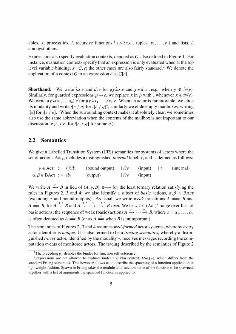
closely follows the mechanism offered by the Erlang Virtual Machine (EVM) [CT09],whereby we choose to only record asynchronous message sends and mailbox messagereceives; see rules SndM and RcvM resp.; in these rules, the tracer actor receives a mes-sage in its mailbox reporting the action, defined through the function3 defined below:

tr(α) def=

{sd, i, v} if α = i!v{rv, i, v} if α = i?v

By contrast, unmonitored actor actions are not traced; see rules SndU and RcvU. Inter-nal communication is not traced either, even when it involves monitored actions, therebylimiting tracing to external interactions (of monitored actors); see rules Com and Par.In Par, the side-condition in Par enforces the single-receiver property of actor systems;for instance, it prevents a transition with an action j!v when actor j is part of the actorsystem B.

Our semantics assumes substitutions, σ ∈ Sub :: Var ⇀ Val, which are partial mapsfrom variables xi to values vi and denoted as {v1, . . . , vn /x1, . . . , xn}. Rules Rd1 and Rd2 (inconjunction with Snd, Rcv and Com) describe how actor communication is not atomic,as opposed to more traditional message-passing semantics [Mil89], but happens in twosteps: an actor first receives a message in its mailbox and then reads it at a later stage.The mailbox reading command includes pattern-matching functionality, allowing theactor to selectively choose which messages to read first from its mailbox whenever apattern from the pattern list is matched; when no pattern is matched, mailbox readingblocks. This differs from pattern matching in case branching, described by the rules Cs1and Cs2: similar to the mailbox read construct, it matches a value to the first appropriatepattern in the pattern list, launching the respective guarded expression with the appro-priate variable bindings resulting from the pattern match; if, however, no match is foundit generates an exception, exit, which aborts subsequent computation, Ext, unless it is

3We elevate tr to basic action sequences s in point-wise fashion, tr(s), where tr(ε) = ε.

8

caught using Ctc.4 Rules Rd1, Rd2, Cs1 and Cs2 make use of the auxiliary functionmtch : PLst × Val→ Exp⊥ defined as follows:

Definition 1 (Pattern Matching) We define mtch and vmtch as follows:

mtch(g, l)def=

⊥ if g = ε

eσ if g = p→ e : f , vmtch(p, v) = σ

d if g = p→ e : f , vmtch(p, v) = ⊥,mtch( f , v) = d⊥ otherwise

vmtch(p, v)def=

∅ if p = v (whenever p is a, i or nil){v/x} if p = x⊎n

i=1 σi if p = {p1, . . . , pn}, v = {v1, . . . , vn} where vmtch(pi, vi) = σi

σ ] {l/x} if p = o : x, v = u : l where vmtch(o, u) = σ

⊥ otherwise

σ1 ] σ2def=

σ1 ∪ σ2 if dom(σ1) ∩ dom(σ2) = ∅

σ1 ∪ σ2 if ∀v ∈ dom(σ1) ∩ dom(σ2).σ1(v) = σ2(v)⊥ if σ1 = ⊥ or σ2 = ⊥

⊥ otherwise

Spawning, using rule Spw, launches a new actor whose scoped identifier is known onlyto the spawning actor, and whose monitoring modality is inherited from the spawningactor when this is either ◦ (monitorable) or • (un-monitorable); if the spawning ac-tor is the tracer process (the ∗ modality), the monitoring modality of the new actor isset to • (un-monitorable). Due to the asynchronous nature of actor communication,scoped actors can send messages to the environment but cannot receive messages fromit. Identifier scope is extended, possibly opened up to external observers, through ex-plicit communication as in standard message-passing systems; see Opn. The functionsin Def. 14 identifies values that include identifiers and thus, extending the identifiersscope. Structural equivalence, A ≡ B, is employed to simplify the presentation of theLTS rules; see rule Str together with Figure 5. The remaining rules in Figure 2 arefairly straightforward.

4In the case of exceptions, let variable bindings x = e, d behave differently from standard let encodingsin terms of call-by-value functions, i.e., λx.d(e), which is why we model them separately.

9

Definition 2 We define obj, subj5 and fId as follows:

obj(γ)def=

∅ if γ = τ

{i} if γ = (~h)i!v or i?v

subj(γ)def=

∅ if γ = τ(idv(v) \ {~h}

)if γ = (~h)i!v

idv(v) if γ = i?v

fId(A)def=

{i} if A = i[e / q]m

fId(B) ∪ fId(C) if A = B ‖ CfId(B) \ {i} if A = (i)(B)

Discussion: Our tracing semantics sits at a slightly higher level of abstraction thanthat offered by the EVM[CT09]. For instance, trace entries typically contain more in-formation. Moreover, in contrast to our semantics, the EVM records internal communi-cation between monitored actors, as an output trace entry immediately followed by thecorresponding input trace entry; here we describe a sanitised trace whereby matchingtrace entries are filtered out. Our tracing semantics is also more restrictive since themonitored actors are fixed: we model a simple (Erlang) monitor instrumentation setupwhereby actors are registered to be monitored upfront before computation commencesor actors that are spawned by other monitored actors. The instrumentation approach isdiscussed in further detail in Section 4.1.

Example 1 (Non-Deterministic behaviour) Actors may exhibit non-deterministic be-haviour as a result of internal choices, but also as a result of external choices [Mil89,HM85]. Consider the actor system:

A , ( j, h, imon)(i[rcv x→ obs!x end / ε]◦ ‖ j[i!v]◦ ‖ h[i!u]◦ ‖ imon[e / q]∗

)According to the semantics defined in Figures 2, 3 and 4, we could have the behaviourwhere actor j sends value v to actor i, (2), i reads it from its mailbox, (3) and subse-quently outputs it to some external actor obs, (4) (while recording the external commu-nication at the monitor’s mailbox as the entry {sd, obs, v}).

Aτ−→ ( j, h, imon)

(i[rcv x→ obs!x end / v]◦ ‖ j[v] ‖ h[i!u] ‖ imon[e / q]∗

)(2)

τ−→ ( j, h, imon)

(i[obs!v / ε]◦ ‖ j[v] ‖ h[i!u] ‖ imon[e / q]∗

)(3)

obs!v−−−−→ ( j, h, imon)

(i[v / ε]◦ ‖ j[v] ‖ h[i!u] ‖ imon[e / q : {sd, obs, v}]∗

)(4)

However, if actor h sends the value u to actor i before actor j, this τ-action would

5The functions idv, ide and idg are defined in the appendix section.

10

amount to an internal choice and we observe the different external behaviour Aobs!u

====⇒ B(for some B); correspondingly the monitor at B would hold the entry {sd, obs, u}.

The actor system A could also receive different external inputs resulting an external

choice. For instance we can derive Ai?v1−−−→ B1 or A

i?v2−−−→ B2 where from B1 we can only

observe the output B1obs!v1

=====⇒ C1 and, dually, B2 can produce the weak external output

B2obs!v2

=====⇒ C2 (for some C1 and C2). Correspondingly, the monitor mailbox at C1 wouldbe appended by the list of entries {rv, i, v1} : {sd, obs, v1} (and dually for C2).

3 A Monitorable Logic for Open Systems

We consider an adaptation of SafeHML (SHML) [AI99], a sub-logic of the Hennessy-Milner Logic (HML) with recursion6 for specifying correctness properties of the actorsystems defined in Section 2. SHML syntactically limits specifications to safety proper-ties which can be monitored at runtime[MP90, CMP92, BLS11].

3.1 Logic

Our logic assumes a denumerable set of formula variables, X,Y ∈ LVar, and is induc-tively defined by the following grammar:

ϕ, ψ ∈ sHML ::= ff | ϕ∧ψ | [α]ϕ | X | max(X, ϕ)

The formulas for falsity, ff, conjunction, ϕ∧ψ, and action necessity, [α]ϕ, are inheriteddirectly from HML[HM85], whereas variables X and the recursion construct max(X, ϕ)are used to define maximal fixpoints; as expected, max(X, ϕ) is a binder for the freevariables X in ϕ, inducing standard notions of open and closed formulas.

We only depart from the standard SHML of [AI99] by limiting necessity formulas tobasic actions α, β ∈ BAct. This is more of a design choice so as keep our technicaldevelopment manageable. The handling of bounded output actions is well understood[MPW93] and do not pose problems to monitoring, apart from making action patternmatching cumbersome. Silent τ labels can also be monitored using minor adaptationsto the monitors we defined later in Section 4; however, they would increase substan-tially the size of the traces recorded, unnecessarily cluttering the tracing semantics ofSection 2.

6HML with recursion has been shown to be as expressive as the µ-calculus[Koz83].

11

3.2 Semantics

The semantics of our logic is defined over sets of actor systems, S ∈ P(Actr). Tradi-tional presentations assume variable environments, ρ ∈ (LVar → P(Actr)), mappingformula variables to sets of actor systems, together with the operation ϕ{ψ/X}, whichsubstitutes free occurances of X in ϕ with ψ without introducing any variable capture,and the operation ρ[X 7→ S ], returning the environment mapping X to S while acting asρ for the remaining variables.

Definition 3 (Satisfaction) For arbitrary variable environment ρ, the set of actors sat-isfying ϕ ∈ sHML, denoted as ~ϕ�ρ, is defined by induction on the structure of ϕ as:

~ff�ρdef= ∅

~ϕ∧ψ�ρdef= ~ϕ�ρ ∩ ~ψ�ρ

~[α]ϕ�ρ def=

{A | B ∈ ~ϕ�ρ whenever A

α==⇒ B

}~X�ρ

def= ρ(X)

~max(X, ϕ)�ρ def=

⋃{S | S ⊆ ~ϕ�ρ[X 7→ S ]}

Whenever ϕ is a closed formula, its meaning is independent of the environment ρ and iswritten as ~ϕ�. When an actor system A satisfies a closed formula ϕ, we write A |=s ϕin lieu of A ∈ ~ϕ�. When restricted to closed formulas, the satisfaction relation |=s canalternatively be specified as Definition 4 (adapted from [AI99].)

Definition 4 (Satisfiability) A relation R ∈ Actr × sHML is a satisfaction relation iff:

(A, ff) ∈ R never(A, ϕ∧ψ) ∈ R implies (A, ϕ) ∈ R and (A, ψ) ∈ R

(A, [α]ϕ) ∈ R implies (B, ϕ) ∈ R whenever Aα

==⇒ B(A,max(X, ϕ)) ∈ R implies (A, ϕ{max(X, ϕ)/X}) ∈ R

Satisfiability, |=s, is the largest satisfaction relation; we write A |=s ϕ in lieu of (A, ϕ) ∈ sat.7

Example 2 (Satisfiability) SHML formulas specify safety properties i.e., prohibited be-haviours that should not be exhibited by satisfying actors. Consider the formula

ϕex , max(X, [α][α][β]ff∧ [α]X ) (5)

7It follows from standard fixed-point theory that the implications of satisfaction relation are bi-implications for Satisfiability.

12

stating that a satisfying actor system cannot perform a sequence of two external actionsα followed by the external action β (through the subformula [α][α][β]ff), and that thiscondition needs to hold after every α action (through the subformula [α]X); effectivelythe formula states that any sequence of external actions α that is greater than two cannotbe followed by an external action β.

An actor system A1 exhibiting (just) the external behaviour A1αβ

==⇒ A′1 for arbitrary A′1satifies ϕex, just as an actor system A2 with (infinite) behaviour A2

α=⇒ A2. An actor sys-

tem A3 with an external action trace A3ααβ

===⇒ A′3 cannot satify ϕex; if, however, (through

some internal choice) it exhibits an alternate external behaviour such as A3β

=⇒ A′′3 wecould not observe any violation since the external trace β is allowed by ϕex.

Because of the potenially non-deterministic nature of actors which may violate a prop-erty along one execution trace but satify it along another, we define a violation relation,Def. 5, characterising actors that violate a property along a specific violating trace.

Definition 5 (Violation) The violation relation, denoted as |=v, is the least relation ofthe form (Actr × Act∗ × sHML) satisfying the following rules:8

A, s |=v ff alwaysA, s |=v ϕ∧ψ if A, s |=v ϕ or A, s |=v ψ

A, αs |=v [α]ϕ if Aα

==⇒ B and B, s |=v ϕ

A, s |=v max(X, ϕ) if A, s |=v ϕ{max(X, ϕ)/X}

Example 3 (Violation) Recall the safety formula ϕex defined in (5). Actor A3, fromEx. 2, together with the witness violating trace ααβ violate ϕex, i.e., (A3, ααβ) |=v ϕex.However, A3 together with trace β do not violate ϕex, i.e., (A3, β) 6|=v ϕex. Def 5 relatesa violating trace with an actor only when that trace leads the actor to a violation. Forinstance, if A3 cannot perform the trace αααβ then we have(A3, αααβ) 6|=v ϕex accordingto Def 5, even though the trace is prohibited by ϕex. Moreover, a violating trace maylead an actor system to a violation before the end of the trace is reached; for instance,we can show that (A3, ααβα) |=v ϕex according to Def 5.

Although it is more convenient to work with Def 5 when reasoning about runtime mon-itors, we still have to show that it corresponds to the dual of Def. 4.

Theorem 1 (Correspondence) ∃s.A, s |=v ϕ iff A 6|= ϕ

8We write A, s |=v ϕ in lieu of (A, s, ϕ) ∈ |=v. It also follows from standard fixed-point theory that theconstrainst of the violation relation are biimplications.

13

Proof For the if case we prove the contrapositive, namely that

∀s.A, s 6|=v ϕ implies A |=s ϕ

by showing that the relation

R = {(γ, ϕ) | ∀s.A, s 6|=v ϕ}

is a satisfaction relation. The proof proceeds by induction on the structure of ϕ:

ff: Contradiction, because from Def. 5 we know we can never have A, s 6|=v ff for any s.

ϕ∧ψ: From the definition ofRwe know that ∀s.A, s 6|=v ϕ∧ψ and, by Def. 5, this impliesthat ∀s.

(A, s 6|=v ϕ and A, s 6|=v ψ

). Distributing the universal quantification yields

∀s.A, s 6|=v ϕ (6)∀s.A, s 6|=v ψ (7)

and by the definition of R, (6) and (7) we obtain (A, ϕ) ∈ R and (A, ψ) ∈ R, asrequired for satisfiability relations by Def. 4.

[α]ϕ: From the definition of R we know that ∀s.A, s 6|=v [α]ϕ. In particular, for alls = αt, we know that ∀t.A, αt 6|=v [α]ϕ. From Def. 5 it must be the case thatwhenever A

α==⇒ B we have that ∀t.B, t 6|=v ϕ, which in turn implies that (B, ϕ) ∈ R

(from the definition of R); this is the implication required by Def. 4.

max(X, ϕ): From the definition of R we know that ∀s.A, s 6|=v max(X, ϕ). For each s,from A, s 6|=v max(X, ϕ) and Def. 5 we obtain A, s 6|=v ϕ{max(X, ϕ)/X} and thus, fromthe definition of R, we conclude that (A, ϕ{max(X, ϕ)/X}) ∈ R as required by Def. 4.

For the only-if case we prove

∃s.A, s |=v ϕ implies A 6|= ϕ

by rule induction on A, s |=v ϕ. Note that A 6|= ϕ means that there does not exist anysatisfiability relation including the pair (A, ϕ).

A, s |=v ff: Immediate by Def. 4.

A, s |=v ϕ∧ψ because A, s |=v ϕ: By A, s |=v ϕ and I.H. we obtain A 6|= ϕ. As a result,we conclude that A 6|= ϕ∧ψ.

A, s |=v ϕ∧ψ because A, s |=v ψ: Similar.

14

A, s |=v [α]ϕ because s = αs′, Aα

==⇒ B and B, s′ |=v ϕ: By B, s′ |=v ϕ and I.H. we obtainB 6|= ϕ, and subsequently, by A

α==⇒ B, we conclude that A 6|= [α]ϕ.

A, s |=v max(X, ϕ) because A, s |=v ϕ{max(X, ϕ)/X}: By A, s |=v ϕ{max(X, ϕ)/X} and I.H. weobtain A 6|= ϕ{max(X, ϕ)/X} which, in turn, implies thatA 6|= max(X, ϕ). �

Def. 5 allows us to show that SHML is a safety language as defined in [MP90, CMP92];this relies on the standard notion of trace prefixes i.e., s ≤ t iff ∃.s′ such that t = ss′.

Theorem 2 (Safety Relation) A, s |=v ϕ and s ≤ t implies A, t |=v ϕ

Proof By Rule Induction on A, s |=v ϕ:

A, s |=v ff: Immediate.

A, s |=v ϕ∧ψ because A, s |=v ϕ: By A, s |=v ϕ, s ≤ t and I.H. we obtainA, t |=v ϕ which, by the same rule, implies A, t |=v ϕ∧ψ.

A, s |=v ϕ∧ψ because A, s |=v ψ: Similar.

A, s |=v [α]ϕ because s = αs′, Aα

==⇒ B and B, s′ |=v ϕ: From s = αs′ and s ≤ t weknow

t = αt′ (8)s′ ≤ t′ (9)

By (9), B, s′ |=v ϕ and I.H. we obtain B, t′ |=v ϕ and by Aα

==⇒ B and (8) we deriveA, t |=v [α]ϕ.

A, s |=v max(X, ϕ) because A, s |=v ϕ{max(X, ϕ)/X}: By A, s |=v ϕ{max(X, ϕ)/X}, s ≤ t andI.H. we obtain A, t |=v ϕ{max(X, ϕ)/X} which implies A, t |=v max(X, ϕ) by the samerule. �

4 Runtime Verifying SHML properties

We define a translation from SHML formulas of Section 3 to programs from Section 2that act as monitors, analysing the behaviour of a system and flagging an alert wheneverthe property denoted by the respective formula is violated by the current execution of the

15

system. Apart from the language translated into, our monitors differ from tests, as de-fined in [AI99], in a number of ways. Firstly, they monitor systems asynchronously andact on traces. By contrast, tests interact with the system directly (potentially inducingcertain system behaviour). More importantly, however, we impose stronger detectionrequirements on monitors as opposed to those defined for test in [AI99]: whereas testsare required to have one possible execution that detects property violations, we requiremonitors to flag violations whenever they occur.9

In terms of our logic, the stronger monitoring requirements are particularly pertinentto conjunction formulas, ϕ1∧ϕ2, whereby a monitor needs to ensure that neither ϕ1

nor ϕ2 are violated. Concurrent monitoring for the subformula ϕ1 and ϕ2 provides anatural translation in terms of the language presented in Section 2, bringing with it theadvantages discussed the Introduction.

Conjunction formulas arise frequently in cases where systems are subject to numerousrequirements from distinct parties. Although the various requirements ϕ1, . . . , ϕn cansometimes be consolidated into a formula without top-level conjunction, it is often con-venient to just monitor for an aggregate formula of the form ϕ1∧ . . .∧ϕn, which wouldtranslate to n concurrent monitors each analysing the system trace independently.

Example 4 (Conjunction Formulas) Consider the formula the two independent for-mulas

ϕno dup ans , [αcall](max(X, [αans][αans]ff∧[αans][αcall]X)

)(10)

ϕreact ans , max(Y, [αans]ff∧[αcall][αans]Y) (11)

Formula ϕno dup ans requires that call actions αcall are at most serviced by a single answeraction αans, whereas ϕreact ans requires that answer actions are only produced in responseto call actions. Even though it is possible to rephrase the conjunction of the two for-mulas as a single formula without a top-level conjunction, it is more straightforward tomonitor for ϕno dup ans∧ϕreact ans using two parallel monitors, one for each subformula.10

Moreover, multiple conjunctions arise indirectly when they are used under fixpoint op-erators in formulas.

Example 5 (Conjuctions and Fixpoints) Recall ϕex, defined in (5) in Ex. 2. Seman-tically, the formula represents the infinite tree depicted in Figure 6(a), comprising of

9There are other discrepancies such as the fact that monitors are required to keep overheads to aminimum, whereas tests typically are not.

10In cases where distinct parties are responsible for each subformula, keeping the subformulas separatemay also facilitate maintainability and increases separation of concerns.

16

∧

[α]

[α]

[β]

ff

[α]

∧

[α]

[α]

[β]

ff

[α]

∧

......

(a) Denotation of ϕex definedin (5)

∧

[α]

[α]

[β]

ff

[α]

X 7→ ϕ

(b) Constructedmonitor for ϕex whereϕ = [α][α][β]ff∧[α]X

∧

[α]

[α]

[β]

ff

[α]

∧

[α]

[α]

[β]

ff

[α]

X 7→ ϕ

(c) First expansion of theconstructed monitor for ϕex

Figure 6: Monitor Combinator generation

17

an infinite number of conjunctions. Although in practice, we cannot generate an infinitenumber of concurrent monitors, ϕex will translate into a number of concurrent monitors.

Monitor synthesis (~−�m : sHML → Exp) described in Def. 6, returns functions thatare parametrised by a map (encoded as a list of tuples) from formula variables to othersynthesised monitors of the same form; the map encodes the respective variable bindingsin a formula and is used for formula recursive unrolling. We only limit monitoring toclosed, guarded11 sHML formulas: monitor instrumentation, performed through thefunction M defined below, spawns the synthesised function applied to the empty map,nil, and then acts as a message forwarder to the spawned process, mLoop, for the traceit receives through the tracing semantics of Section 2.2.

M def= λxfrm.zpid = spw

(~xfrm�

m(nil)), mLoop(zpid)

mLoop def= µyrec.λxpid.rcv z→ xpid!z end, yrec(xpid)

Definition 6 (Monitors)

~ff�m def= λxenv.sup!fail

~ϕ∧ψ�m def=

λxenv. ypid1 = spw

(~ϕ�m(xenv)

),

ypid2 = spw(~ψ�m(xenv)

),

fork(ypid1, ypid2)

~[α]ϕ�m def=

λxenv.rcv tr(α) → ~ϕ�m(xenv);

→ okend

~max(X, ϕ)�m def= λxenv. ~ϕ�

m({′X′, ~ϕ�m} : xenv)

~X�m def=

λxenv. ymon = lookUp(′X′, xenv),ymon(xenv)

11In guarded SHML formulas, formula variables appear only as a subformula of a necessity formula.

18

Auxiliary Function definitions and meta-operators:

forkdef= µyrec.λ(xpid1, xpid2).rcv z→

(xpid1!z, xpid2!z

)end, yrec(xpid1, xpid2)

lookUpdef=

µyrec.λ(xvar, xmap).case xmap of({xvar, zmon} : ) → zmon

: ztl → yrec(xvar, ztl)nil → exit

end

In Def. 6, the monitor translation for ff immediately reports a violation by sending themessage fail to a predefined actor sup handling the violation. The translation of ϕ1∧ϕ2

consists in spawning the respective monitors for ϕ1 and ϕ2 and then forwarding the tracemessages to these spawned monitors through the auxiliary function fork. The translatedmonitor for [α]ϕ behaves as the monitor translation for ϕ once it receives a trace messageencoding the occurrence of action α (see meta-function tr(−)), but terminates if the tracemessage does not correspond to α.

The translations of max(X, ϕ) and X are best understood together: the monitor formax(X, ϕ) behaves like that for ϕ, under the extended map where X is mapped to themonitor for ϕ, effectively modelling the formula unrolling ϕ{max(X, ϕ)/X} from Def. 4;the monitor for X retrieves the monitor translation for the formula it is bound to in themap through using function lookUp, and behaves like this monitor. The assumption thatsynthesised formulas is closed guarantees that map entries are always found by lookUp,whereas the assumption regarding guarded formulas guarantees that monitor executionsdo not produce infinite bound-variable expansions.

Example 6 (Monitor Translation) The generated monitor for ϕex, defined in (5), is

Moni to r = m max ( ’X’ ,m and ( m nec send ( alphaTo , alphaMsg

m nec send ( alphaTo , alphaMsg ,m nec send ( betaTo , betaMsg , m f l s ( ) ) ) ) ,

m nec send ( alphaTo , betaMsg , m var ( ’X ’ ) ) ) ) ,M( Moni to r ) .

where the referenced functions are defined as

m f l s ( ) → fun ( Mappings ) → sup ! f a i l end .

m n e c r e c v ( Rece ive r , Message , Ph i ) →fun ( Mappings ) →

r e c e i v e{ a c t i o n , { recv , Rece ive r , Message } } → Phi ( Mappings ) ;

19

{ a c t i o n , } → okend

end .

m nec send ( To , Message , Ph i ) →fun ( Mappings ) →

r e c e i v e{ a c t i o n , { send , SentFrom , To , Message } } → Phi ( Mappings ) ;{ a c t i o n , } → ok

endend .

m and ( Phi1 , Ph i2 ) →fun ( Mappings ) →

A = spawn ( fun ( ) → Phi1 ( Mappings ) ) ,B = spawn ( fun ( ) → Phi2 ( Mappings ) ) ,f o r k (A, B)

end .

f o r k (A, B) → r e c e i v e Msg →A ! Msg ,B ! Msg

end ,f o r k (A, B ) .

m max ( Var , Ph i ) → fun ( Mappings ) →Phi ( [ { Var , Ph i } | Mappings ] )

end .

m var ( Var ) → fun ( Mappings ) →Moni to r = lookUp ( Var , Mappings ) ,Moni to r ( Mappings )

end .

lookUp ( Var , Mappings ) →case Mappings o f

[ { Var , Moni to r } | O t h e r ] → Moni to r ;[ | T a i l ] → lookUp ( Var , T a i l ) ;[ ] → e x i t

end .

The code in this example first creates the structure of functions that together representthe property that is being verified. The functions called m_form are the direct Erlangtranslation from the Def. 6. The process M is responsible to start up the monitor forthe property generated through the call to these monitor functions and forwarding thetrace messages to these monitors. When spawning the monitor for the property, theproperty is passed an empty environment. The function for the maximum fixpoint ex-tends this environment with a reference to the definition of the property itself and con-

20

tinues to execute the remaining property. When a free instance of the variable X isencountered, the monitor definition is retrieved from the environment using the func-tion lookUp(Var, Mappings) and continues executing as the result of this function.Thus, the actor executing the property for X evolves to an ∧ node while spawning twonew actors, one checking for the subformula [α][α][β]ff, and another one checking forthe formula [α]X. This is depicted in Figure 6(c). Whenever the monitor for the vari-able X is encountered following a sequence of received traces, the same unfolding isrepeated by the rightmost actor in Figure 6(c), thereby increasing the monitor overheadincrementally, as required by the runtime behaviour of the system being monitored.

4.1 Tool Implementation

The monitor generation procedure given in Def. 6 acts as a basis for a prototype imple-mentation of a tool automating monitor synthesis of sHML formula into actual Erlangmonitors. The tool can be downloaded from [Sey13]. Several design decisions weretaken while implementing the tool so as to integrate and instrument the system with thegenerated monitors.

As discussed earlier, we make use of the tracing mechanism that is available in the EVMto gather the trace of a particular process. However, when monitoring a system, we needto collect traces from a collection of processes that are communicating with each otherand also with external processes. In Erlang, the tracing functionality is enabled usingthe trace/2 built-in function where the first argument is the process identifier to traceand the second parameter is a list of flags to specify the type of tracing required. Oneof the flags that is used in our tool is called set_on_spawn that enables tracing onnewly spawned processes. This flag’s behaviour matches the language semantics in therule Spw since if the process spawning a new child process is traceable, the new childprocess is also traceable.

Another challenge that arose when instrumenting the system was that of the approachto use so as to initialise the monitoring tool. The ideal way to initialise the monitor isto enable the monitoring while the system is already executing. In order to be able todo so, a list of all the PIDs of the processes in the system being monitored is required.In order to avoid the race-condition where new processes are spawned while enablingtracing, it would be necessary to suspend the execution of the system through someinstrumentation mechanism. Instead, our tool provides the monitor with the functionthat needs to be called when starting up the system. The monitor spawns a specialinitiator process that blocks its execution immediately using the receive construct. Themonitor then enables the tracing for this newly spawned process with the setting of theset_on_spawn flag, after which it notifies the process that it can resume its executionand start up the system. The result of this setup is that all processes spawned by the

21

system are monitored as well.12

After instrumenting the system to receive trace messages for its actions, the actual mon-itoring needs to take place. The user specifies the correctness property using the sHMLlogic introduced in Section 3. Hence, a parser is also provided in order to translate theproperty in sHML to the actual synthesis presented in this study. This synthesis is usedafter the instrumentation is in place in order to monitor the system for violating traces.

5 Correctness

We now discuss how, in the model of the runtime system, monitors are instrumented toexecute wrt. monitored systems, Section 5.1, how correct monitor behaviour is specifiedin such a setting, Section 5.2.

5.1 System Instrumentation

We limit monitoring to monitorable systems, Def. 7, whereby all actors of a systemare monitorable. This guarantees that all the basic actions produced by the system arerecorded as trace entries at the monitor’s mailbox; note that due to the asynchronousnature of communication, even scoped actors can generate visible actions by sendingmessages to other actors in the environment. An important property for our monitoringsetup is that monitorable systems are closed wrt. weak sequences of basic actions;this is essential for our instrumentation to remain valid over the course of a monitoredexecution.

Definition 7 (Monitorable Systems) An actor system A is said to be monitorable iff

A ≡ (h)(i[e / q]m ‖ B

)implies m = ◦

Lemma 1 A is monitorable and A‖ i[e / q]∗s

=⇒ B‖ i[e′ / q′]∗ implies B is monitorable

Proof By induction on the length of As

==⇒ B and then by rule induction for the inductivecase. Note that in rule Spw, the spawned process inherits the monitoring modality ofthe process spawning it. Since in a monitorable system, all actors are monitored, newspawned actors will be set with a monitorable modality as well. �

12The blocking is necessary so as to prevent the system from spawning new processes that are notmonitored and resulting in the same race condition as before.

22

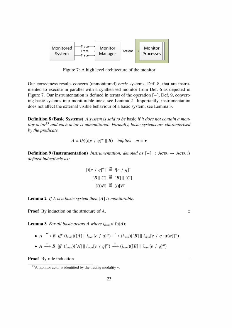
Figure 7: A high level architecture of the monitor

Our correctness results concern (unmonitored) basic systems, Def. 8, that are instru-mented to execute in parallel with a synthesised monitor from Def. 6 as depicted inFigure 7. Our instrumentation is defined in terms of the operation d−e, Def. 9, convert-ing basic systems into monitorable ones; see Lemma 2. Importantly, instrumentationdoes not affect the external visible behaviour of a basic system; see Lemma 3.

Definition 8 (Basic Systems) A system is said to be basic if it does not contain a mon-itor actor13 and each actor is unmonitored. Formally, basic systems are characterisedby the predicate

A ≡ (h)(i[e / q]m ‖ B

)implies m = •

Definition 9 (Instrumentation) Instrumentation, denoted as d−e :: Actr → Actr isdefined inductively as:

di[e / q]medef= i[e / q]◦

dB ‖ Cedef= dBe ‖ dCe

d(i)Be def= (i)dBe

Lemma 2 If A is a basic system then dAe is monitorable.

Proof By induction on the structure of A. �

Lemma 3 For all basic actors A where imon < fn(A):

• Aα−−−→ B iff (imon)

(dAe ‖ imon[e / q]m) α

−−−→ (imon)(dBe ‖ imon[e / q : tr(α)]m)

• Aτ−−→ B iff (imon)

(dAe ‖ imon[e / q]m) τ

−−→ (imon)(dBe ‖ imon[e / q]m)

Proof By rule induction. �

13A monitor actor is identified by the tracing modality ∗.

23

5.2 Monitor Correctness

Specifications relating to monitor correctness are complicated by two factors: systemnon-determinism and system divergence. We deal with the non-determinism of the mon-itored system by requiring proper monitor behaviour only when the system performs aviolating execution; this can be expressed through the violation relation formalised inDef. 5.

System divergence however complicates statements relating to any deterministic de-tection behaviour expected from the synthesised monitor should the monitored systemperform a violating execution: although we would like to require that the monitor mustalways detect and flag a violation whenever it occurs, a divergent system executingin parallel with it can postpone indefinitely this behaviour. Even though we have noguarantees on the behaviour of the system being monitored, the EVM provides fair-ness guarantees[CT09] for actor executions. In such cases, it therefore suffices to re-quire a weaker property from our synthesised monitors, reminiscent of the condition infair/should-testing[RV07].

Definition 10 (Should-α) A ⇓αdef=

(A ===⇒ B implies B

α==⇒

)Definition 11 (Correctness) e ∈ Exp is a correct monitor for ϕ ∈ sHML iff for anybasic actors A ∈ Actr, i < fId(A), and execution traces s ∈ Act∗ \ {sup!fail}:

(i)(dAe ‖ i[e]∗

) s=⇒ B implies

(A, s |=v ϕ iff B ⇓sup!fail

)6 Proving Correctness

Def. 11, defined in the previous section, allows us to state the main result of the paper,Theorem 3.

Theorem 3 (Correctness) For all ϕ ∈ sHML, M(ϕ) is a correct monitor for ϕ.

Proving Theorem 3 directly can be an arduous task because it requires reasoning aboutall the possible execution paths of the monitored system in parallel with the instru-mented monitor. Instead we propose a technique that teases apart three sub-propertiesabout our synthesised monitors from the correctness property of Theorem 3. As arguedin the Introduction, these sub-properties can be checked by distinct analysing entities orused as vetting checks so as to abort early our correctness analysis. More importantly,together, these weaker properties imply the stronger property of Theorem 3.

24

The first sub-property is Violation Detection, Lemma 4, guaranteeing that for everyviolating trace s of formula ϕ there exists an execution by the respective synthesisedmonitor that detects the violation. This property is easier to verify than Theorem 3because it requires us to consider the execution of the monitor in isolation and, moreimportantly, requires us to verify the existence of a single execution path that detects theviolation; concurrent monitors typically have multiple execution paths.

Lemma 4 (Violation Detection) For basic A ∈ Actr and imon < fId(A), As

==⇒ implies:

A, s |=v ϕ iff imon[M(ϕ) / tr(s)]∗sup!fail

=====⇒

Unlike Lemma 4, the next property, called Detection Preservation (Lemma 5), is notconcerned with relating detections to actual violations; instead it guarantees that if amonitor can potentially detect a violation, further reductions do not exclude the possi-bility of this detection. In the case where monitors always have a finite reduction wrt.their mailbox contents (as it turns out to be the case for the monitors given in Def. 6) thiscondition suffices to guarantee that the monitor will deterministically detect violations.More generally, however, in a setting that guarantees fair actor executions, Lemma 5ensures that detection will always eventually occur, even when monitors execute in par-allel with other, potentially divergent, systems.

Lemma 5 (Detection Preservation) For all ϕ ∈ sHML, q ∈ Val∗

imon[M(ϕ) / q]∗sup!fail

=====⇒ and imon[M(ϕ) / q]∗ ===⇒ B implies Bsup!fail

=====⇒

The third sub-property we require is Separability, Lemma 6, which implies that the be-haviour of a (monitored) system is independent of the monitor and, dually, the behaviourof the monitor depends, at most, on the trace generated by the system.

Lemma 6 (Monitor Separability) For all basic actors A ∈ Actr, imon < fId(A), ϕ ∈sHML, s ∈ Act∗ \ {sup!fail},

(imon)(dAe ‖ imon[M(ϕ)]∗

) s=⇒ B implies ∃B′, B′′s.t.

B ≡ (imon)

(B′ ‖ B′′

)A

s=⇒ A′ s.t. B′ = dA′e

imon[M(ϕ) / tr(s)]∗ =⇒ B′′

These three properties suffice to show monitor correctness.

25

Recall Theorem 3 (Monitor Correctness). For all ϕ ∈ sHML, basic actors A ∈ Actr,imon < fn(A), s ∈ Act∗ \ {sup!fail}, whenever (imon)

(dAe ‖ imon[M(ϕ)]∗

) s=⇒ B then:

A, s |=v ϕ iff B ⇓sup!fail

Proof For the only-if case, we assume

(imon)(A ‖ imon[M(ϕ)]∗

) s=⇒ B (12)

A, s |=v ϕ (13)

From Def. 10 we can further assume

B =⇒ B′ (14)

and then be required to prove that B′sup!fail====⇒. From (12) (14) and Lemma 6 we know

∃B′′, B′′′s.t. B′ = (imon)(B′′ ‖ B′′′

)(15)

As

==⇒ A′ for some A′ where dA′e = B′′ (16)imon[M(ϕ) / tr(s)]∗ ===⇒ B′′′ (17)

From (16), (13) and Lemma 4 we obtain

imon[M(ϕ) / tr(s)]∗sup!fail

=====⇒ (18)

and from (17), (18) and Lemma 5 we obtain B′′′sup!fail

=====⇒ and hence, by (15), and by rules

Par and Scp, we obtain B′sup!fail

=====⇒, as required.

For the if case we know:


) s==⇒ B (19)

B ⇓sup!fail (20)

and have to prove that A, s |=v ϕ. From (20) we know Bsup!fail

=====⇒ which, together with(19) implies

∃B′ s.t. (imon)(dAe ‖ imon[M(ϕ)]∗

) s==⇒ B′

sup!fail−−−−−−→ (21)

26

From Lemma 6 and (21) we obtain

∃B′′, B′′′s.t. B′ = (imon)(B′′ ‖ B′′′

)(22)

As

==⇒ A′ for some A′ where dA′e = B′′ (23)imon[M(ϕ) / tr(s)]∗ ==⇒ B′′′ (24)

From (21), (22) and the freshness of sup!fail to A we deduce that B′′sup!fail−−−−−→, and subse-

quently, by (24), we obtain

imon[M(ϕ) / tr(s)]∗sup!fail====⇒ (25)

Finally, by (23), (25) and Lemma 4 we obtain A, s |=v ϕ, as required. �

6.1 Proofs of the Sub-Properties

In this section we detail the proofs of the individual sub-properties identified in Sec. 6;on first reading, the reader may safely skip this section.

6.1.1 Violation Detection

The first sub-property we consider is Lemma 4, Violation Detection. One of the mainLemmas used in the proof, namely Lemma 10, relies on an encoding of formula sub-stitutions, θ :: LVar⇀ sHML, partial maps from formula variables to (possibly open)formulas, to lists of tuples containing a string representation of the variable and therespective monitor translation of the formula as defined in Def. 6. Formula substitu-tions are denoted as lists of individual substitutions, {ϕ1/X1} . . . {ϕn/Xn} where every Xi isdistinct, and empty substitutions are denoted as ε.

Definition 12 (Formula Substitution Encoding)

enc(θ) def=

nil when θ = ε

{′X′, ~ϕ�m} : enc(θ′) if θ = {max(X, ϕ)/X}θ′

We can show that our monitor lookup function of Def. 6 models variable substitution,Lemma 7. We can also show that different representations of the same formula substi-tution do not affect the outcome of the execution of lookUp on the respective encoding,which justifies the abuse of notation in subsequent proofs that assume a single possiblerepresentation of a formula substitution.

27

Lemma 7 θ(X) = ϕ implies i[lookUp(′X′, enc(θ)) / q]m ===⇒ i[~ϕ�m / q]m

Proof By induction on the number of mappings {ϕ1/X1} . . . {ϕn/Xn} in θ. �

Lemma 8 If θ(X) = ϕ then i[lookUp(′X′, enc(θ′)) / q]m ===⇒ i[~ϕ�m / q]m whenever θand θ′ denote the same substitution.

Proof By induction on the number of mappings {ϕ1/X1} . . . {ϕn/Xn} in θ. �

In one direction, Lemma 4 relies on Lemma 10 in order to establish the correspondencebetween violations and the possibility of detections; this lemma, in turn, uses Lemma 9which relates possible detections by monitors synthesised from subformulas to possibledetections by monitors synthesised from conjunctions using these subformulas.

Lemma 9 For an arbitrary θ, (i)(imon[mLoop( j1) / tr(s)]∗ ‖ i[~ϕ1�

m(enc(θ))]•) sup!fail

====⇒

implies (i)(imon[mLoop(i) / tr(s)]∗ ‖ i[~ϕ1∧ϕ2�

m(enc(θ))]•) sup!fail

====⇒ for any ϕ2 ∈ sHML.

Proof By Def. 6 we know that

(i)(imon[mLoop(i) / tr(s)]∗ ‖ i[~ϕ1∧ϕ2�

m(enc(θ))]•)

==⇒

(i)(imon[mLoop(i) / tr(s)]∗ ‖ ( j, h)

(i[fork( j, h)]• ‖ j[~ϕ1�

m(enc(θ))]• ‖ h[~ϕ2�m(enc(θ))]•

))We then prove by induction the structure of s that

(i)(imon[mLoop(i) / tr(s)]• ‖ i[~ϕ1�

m(enc(θ)) / q]•) sup!fail

====⇒ implies

(i)(

imon[mLoop(i) / tr(s)]∗ ‖( j, h)

(i[fork( j, h)]• ‖ j[~ϕ1�

m(enc(θ)) / q]• ‖ h[~ϕ2�m(enc(θ)) / q]•

) )sup!fail====⇒

s = ε: From Def. 6 we know that imon[mLoop(i) / ε]• in the system(i)

(imon[mLoop(i) / tr(s)]• ‖ i[~ϕ1�

m(enc(θ)) / q]•)

is stuck (after one τ-transition).

Thus it must have been the case that i[~ϕ1�m(enc(θ)) / q]•

sup!fail====⇒. The result thus

follows by repeated applications of rules Par and Scp.

s = αt: We have two subcases to consider. Either i[~ϕ1�m(enc(θ)) / q]•

sup!fail====⇒ immedi-

ately, in which case the result follows analogously to the previous case. Alterna-tively, we have

(i)(imon[mLoop(i) / tr(α) : tr(t)]∗ ‖ i[~ϕ1�

m(enc(θ)) / q]•)

==⇒

(i)(imon[mLoop(i) / tr(t)]∗ ‖ i[~ϕ1�

m(enc(θ)) / q : tr(α)]•) sup!fail

====⇒(26)

28

By (26) and I.H. we obtain

(i)

imon[mLoop(i) / tr(t)]∗ ‖

( j, h)(

i[fork( j, h)]• ‖j[~ϕ1�

m(enc(θ)) / q : tr(α)]• ‖ h[~ϕ2�m(enc(θ)) / q : tr(α)]•

) sup!fail====⇒

and the result follows from the fact that

(i)(

imon[mLoop(i) / tr(s)]∗ ‖( j, h)

(i[fork( j, h)]• ‖ j[~ϕ1�

m(enc(θ)) / q]• ‖ h[~ϕ2�m(enc(θ)) / q]•

) )==⇒

(i)

imon[mLoop(i) / tr(t)]∗ ‖

( j, h)(

i[fork( j, h)]• ‖j[~ϕ1�

m(enc(θ)) / q : tr(α)]• ‖ h[~ϕ2�m(enc(θ)) / q : tr(α)]•

) �

Lemma 10 If A, s |=v ϕθ and lenv = enc(θ) then

(i)(imon[mLoop(i) / tr(s)]∗ ‖ i[~ϕ�m(lenv)]•

) sup!fail=====⇒ .

Proof Proof by rule induction on A, s |=v ϕθ:

A, s |=v ffθ: Using Def. 6 for the definition of ~ff�m and the rule App (and Par and Scp),we have

(i)(imon[mLoop(i) / tr(s)]∗ ‖ i[~ff�m(lenv)]•) ==⇒ (i)(imon[mLoop(i) / tr(s)]∗ ‖ i[sup!fail]•)

The result follows trivially, since the process i can transition with a sup!fail actionin a single step using the rule SndU.

A, s |=v (ϕ1∧ϕ2)θ because A, s |=v ϕ1θ: By A, s |=v ϕ1θ and I.H. we have

(i)(imon[mLoop(i) / tr(s)]∗ ‖ i[~ϕ1�m(lenv)]•)

sup!fail====⇒

The result thus follows from Lemma 9, which allows us to conclude that

(i)(imon[mLoop(i) / tr(s)]∗ ‖ i[~ϕ1∧ϕ2�m(lenv)]•)

sup!fail====⇒

A, s |=v (ϕ1∧ϕ2)θ because A, s |=v ϕ2θ: Analogous.

A, s |=v ([α]ϕ)θ because s = αt, Aα

==⇒ B and B, t |=v ϕθ: Using the rule App Scp and Def. 6

29

for the property [α]ϕ we derive (27), by executing mLoop— see Def. 6 — we ob-tain (28), and then by rule Rd1 we derive (29) below.

(i)(imon[mLoop(i) / tr(αt)]∗ ‖ i[~ϕ�m(lenv)]•

) τ−−→ (27)

(i)(imon[mLoop(i) / tr(αt)]∗ ‖ i[rcv (tr(α)→ ~ϕ�m(lenv) ; → ok) end]•

)==⇒ (28)

(i)(imon[mLoop(i) / tr(t)]∗ ‖ i[rcv (tr(α)→ ~ϕ�m(lenv) ; → ok) end / tr(α)]•

) τ−−→

(29)

(i)(imon[mLoop(i) / tr(t)]∗ ‖ i[~ϕ�m(lenv)]•

)By B, t |=v ϕθ and I.H. we obtain

(i)(imon[mLoop(i) / tr(t)]∗ ‖ i[~ϕ�m(lenv)]•

) sup!fail====⇒

and, thus, the result follows by (27), (28) and (29).

A, s |=v (max(X, ϕ))θ because A, s |=v ϕ{max(X, ϕ)/X}θ: By Def. 6 and App for process i,we derive

(i)(imon[mLoop(i) / tr(s)]∗ ‖ i[~max(X, ϕ)�m(lenv)]•

)==⇒

(i)(imon[mLoop(i) / tr(s)]∗ ‖ i[~ϕ�m({′X′, ~ϕ�m} : lenv)]•

)(30)

Assuming the appropriate α-conversion for X in max(X, ϕ), we note that fromlenv = enc(θ) and Def. 12 we obtain

enc({max(X, ϕ)/X}θ) = {′X′, ~ϕ�m} : lenv (31)

By A, s |=v ϕ{max(X, ϕ)/X}ρ, (31) and I.H. we obtain

(i)(imon[mLoop(i) / tr(s)]∗ ‖ i[~ϕ�m({′X′, ~ϕ�m} : lenv)]•

) sup!fail====⇒ (32)

The result follows from (30) and (32). �

In the other direction, Lemma 4 relies on Lemma 15, which establishes a correspon-dence between violation detections and actual violations, as formalised in Def. 5.

Lemma 15 relies on a technical result, Lemma 14 which allows us to recover a violatingreduction sequence for a subformula ϕ1 or ϕ2 from that of the synthesised monitor ofa conjuction formula ϕ1∧ϕ2. Lemma 14 employs Corollary 1, which in turn relies onthe technical Lemmata 11 and 12, which prove the result for the specific cases were theviolation is generated by the synthesised monitor of ϕ1 and ϕ2 resp..

30

Lemma 11 For some l ≤ n:

( j, h)(i[fork( j, h) / q1

frkq2frk

]•‖ j[~ϕ1�

m(lenv) / q]• ‖ h[~ϕ2�m(lenv) / r]•

)(

τ−−→)n

( j, h)(i[e j,h

fork / q2frk

]•‖ A ‖ B

) sup!fail−−−−−→ because A

sup!fail−−−−−→

for some A ≡ (~j′)(j[e / q′]• ‖ A′

)where j[~ϕ1�

m(lenv) / qq1frk]• ==⇒ A

and some B ≡ (~h′)(h[d / r′]• ‖ B′

)where h[~ϕ2�

m(lenv) / rq1frk]• ==⇒ B

implies ( j)(imon[mLoop( j) / q1

frkq2frk]∗ ‖ j[~ϕ1�

m(lenv) / q]•)(

τ−−→)l sup!fail

−−−−−→

and

( j, h)(i[v, h!v, fork( j, h) / q1

frkq2frk

]•‖ j[~ϕ1�


)(

τ−−→)n

( j, h)(i[e j,h

fork / q2frk

]•‖ A ‖ B

) sup!fail−−−−−→ because A


for some A ≡ (~j′)(j[e / q′]• ‖ A′

)where j[~ϕ1�


and some B ≡ (~h′)(h[d / r′]• ‖ B′

)where h[~ϕ2�


implies ( j)(imon[mLoop( j) / q1

frkq2frk]∗ ‖ j[~ϕ1�

m(lenv) / q]•)(


−−−−−→

Proof We prove both statements simultaneously, by induction on the structure of themailbox at actor imon, (q1

frkq2frk).

(q1frkq2

frk) = ε: We prove the first case; the second case is analogous. From the structureof fork, Def. 6, we know that i

[fork( j, h) / ε

]• will get stuck after the functionapplication, which means that it must be the case that j[~ϕ1�

m(lenv) / q]• ==⇒ A,from which the conclusion holds trivially by Par and Scp.

(q1frkq2

frk) = v : q′′frk: We prove the first case again, and leave the second, analogous caseto the reader. We have two subcases to consider:

• Either j[~ϕ1�m(lenv) / q]• ==⇒ A, independently of the actor at imon. The

proof follows as in the base case.

• Or it is not the case that j[~ϕ1�m(lenv) / q]• ==⇒ A. This means that the

31

reduction sequence can be decomposed as

( j, h) i

[fork( j, h) / (q1

frkq2frk)

]•‖ j[~ϕ1�


(τ−−→)k

( j, h)(i[v, h!v, fork( j, h) / q′′frk

]•‖ (~j′)

(j[e / q′ : v]• ‖ A′′′

)‖ B′′

)(

τ−−→)n−k

(33)

( j, h)(i[e j,h

fork / q′frk]•‖ A ‖ B

) sup!fail−−−−−→

for some k = k1 + k2 + 3, where

j[~ϕ1�m(lenv) / q]• (

τ−→)k1 (~j′)

(j[e / q′]• ‖ A′′′

)(34)

B′′ ≡ (~h′)(h[d / r′]• ‖ B′′′

)where h[~ϕ2�

m(lenv) / r]• (τ−→)k2 B′′. (35)

By (33), (34) and (35) we can reconstruct the reduction sequence

( j, h) i

[v, h!v, fork( j, h) / q′′frk

]•‖ j[~ϕ1�

m(lenv) / q : v]• ‖ h[~ϕ2�m(lenv) / r]•

(τ−−→)n−3

( j, h)(i[e j,h

fork / q′frk]•‖ A ‖ B


By and I.H. we deduce that for l ≤ n − 3

( j)(imon[mLoop( j) / q′′frk]∗ ‖ j[~ϕ1�

m(lenv) / q : v]•)(


−−−−−→

Thus, by preceeding this transition sequence by three additional τ-transitionswe obtain

( j)(imon[mLoop( j) / v : q′′frk]∗ ‖ j[~ϕ1�

m(lenv) / q]•)(


−−−−−→

�

32

Lemma 12 For some l ≤ n:

( j, h)(i[fork( j, h) / q1

frkq2frk

]•‖ j[~ϕ1�


)(

τ−−→)n

( j, h)(i[e j,h

fork / q2frk

]•‖ A ‖ B

) sup!fail−−−−−→ because B


for some A ≡ (~j′)(j[e / q′]• ‖ A′

)where j[~ϕ1�


and some B ≡ (~h′)(h[d / r′]• ‖ B′

)where h[~ϕ2�


implies (h)(imon[mLoop(h) / q1

frkq2frk]∗ ‖ h[~ϕ2�

m(lenv) / r]•)(


−−−−−→

and

( j, h)(i[v, fork( j, h) / q1

frkq2frk

]•‖ j[~ϕ1�


)(

τ−−→)n

( j, h)(i[e j,h

fork / q2frk

]•‖ A ‖ B

) sup!fail−−−−−→ because B


for some A ≡ (~j′)(j[e / q′]• ‖ A′

)where j[~ϕ1�


and some B ≡ (~h′)(h[d / r′]• ‖ B′

)where h[~ϕ2�


implies (h)(imon[mLoop(h) / q1

frkq2frk]∗ ‖ h[~ϕ2�

m(lenv) / r]•)(


−−−−−→

Proof Analogous to the proof of Lemma 11. �

Corollary 1 For some l ≤ n:

( j, h)(i[fork( j, h) / qfrk

]•‖ j[~ϕ1�


)(

τ−−→)n sup!fail

−−−−−→

implies ( j)(imon[mLoop( j) / qfrk]∗ ‖ j[~ϕ1�

m(lenv) / q]•)(


−−−−−→

or (h)(imon[mLoop(h) / qfrk]∗ ‖ h[~ϕ2�

m(lenv) / r]•)(


−−−−−→

Proof Follows from Lemma 11 and Lemma 12 and the fact that i[fork( j, h) / qfrk]•

cannot generate the action sup!fail. �

Lemma 14 uses another technical result, Lemma 13, stating that silent actions are, insome sense, preserved when actor-mailbox contents of a free actor are increased; notethat the lemma only applies for cases where the mailbox at this free actor decreases insize or remains unaffected by the τ-action, specified through the sublist condition q′ ≤ q.

Lemma 13 (Mailbox Increase) (~h)(i[e / q]m ‖ A)τ−−→ (~j)(i[e′ / q′]m ‖ B) where i < ~h

and q′ ≤ q implies (~h)(i[e / q : v]m ‖ A)τ−−→ (~j)(i[e′ / q′ : v]m ‖ B)

33

Proof By rule induction on (~h)(i[e / q]m ‖ A)τ−−→ (~j)(i[e′ / q′]m ‖ B). �

Equipped with Corollary 1 and Lemma 13, we are in a position to prove Lemma 14.

Lemma 14 For some l ≤ n

(i)(imon[mLoop(i) / tr(s)]∗ ‖ ( j, h)

(i[fork( j, h) / tr(t)

]•‖ j[~ϕ1�

m(lenv)]• ‖ h[~ϕ2�m(lenv)]•

))(

τ−−→)k sup!fail

−−−−−→

implies (i)(imon[mLoop(i) / tr(ts)]∗ ‖ i[~ϕ1�

m(lenv)]•)(


−−−−−→

or (i)(imon[mLoop(i) / tr(ts)]∗ ‖ i[~ϕ2�

m(lenv)]•)(


−−−−−→

Proof Proof by induction on the structure of s.

s = ε: From the structure of mLoop, we know that after the function application, theactor imon[mLoop(i)]∗ is stuck. Thus we conclude that it must be the case that

( j, h)(

i[fork( j, h) / tr(t)

]•‖ j[~ϕ1�


)(


−−−−−→

where k = n or k = n − 1. In either case, the required result follows from Corol-lary 1.

s = αs′: We have two subcases:

• If

( j, h)(


]•‖ j[~ϕ1�


)(


−−−−−→

for some k ≤ n then, by Cor. 1 we obtain

( j)(imon[mLoop( j) / tr(t)]∗ ‖ j[~ϕ1�

m(lenv)]•)(


−−−−−→

or (h)(imon[mLoop(h) / tr(t)]∗ ‖ h[~ϕ2�

m(lenv)]•)(


−−−−−→

for some l ≤ k. By Lemma 13 we thus obtain

( j)(imon[mLoop( j) / tr(ts)]∗ ‖ j[~ϕ1�

m(lenv)]•)(


−−−−−→

or (h)(imon[mLoop(h) / tr(ts)]∗ ‖ h[~ϕ2�

m(lenv)]•)(


−−−−−→

as required.

34

• Otherwise, it must be the case that

(i)

imon[mLoop(i) / tr(s)]∗

‖ ( j, h)(


]•‖ j[~ϕ1�


) (τ−−→)k (36)

(i)(

imon[mLoop(i) / tr(s′)]∗

‖ ( j, h)(i[efork / q : tr(α)

]•‖ A

) )(

τ−−→)n−k sup!fail

−−−−−→ (37)

For some k = 3 + k1 where

( j, h)(


]•‖ j[~ϕ1�


)(

τ−−→)k1

( j, h)(i[efork / q

]•‖ A

) (38)

By (38) and Lemma 13 we obtain

( j, h)(

i[fork( j, h) / tr(t) : tr(α)

]•‖ j[~ϕ1�


)(

τ−−→)k1

( j, h)(i[efork / q : tr(α)

]•‖ A

)and by (37) we can construct the sequence of transitions:

(i)

imon[mLoop(i) / tr(s′)]∗

‖ ( j, h)(

i[fork( j, h) / tr(t) :α

]•‖ j[~ϕ1�


) (τ−−→)n−3 sup!fail

−−−−−→

Thus, by I.H. we obtain, for some l ≤ n − 3

(i)(imon[mLoop(i) / tr(tαs′)]∗ ‖ i[~ϕ1�

m(lenv)]•)(


−−−−−→

or (i)(imon[mLoop(i) / tr(tαs′)]∗ ‖ i[~ϕ2�

m(lenv)]•)(


−−−−−→

The result follows since s = αs′. �

Lemma 15 If As

==⇒, lenv = enc(θ) and (i)(imon[mLoop(i) / tr(s)]∗ ‖ i[~ϕ�m(lenv)]•

) sup!fail====⇒

then A, s |=v ϕθ, whenever fv(ϕ) ⊆ dom(θ).

Proof By strong induction on (i)(imon[mLoop(i) / tr(s)]∗ ‖ i[~ϕ�m(lenv)]•

)(τ−→)n sup!fail

−−−−−→.

n = 0: By inspection of the definition for mLoop, and by case analysis of ~ϕ�m(lenv)

35

from Def. 6, it can never be the case that

(i)(imon[mLoop(i) / tr(s)]∗ ‖ i[~ϕ�m(lenv)]•


Thus the result holds trivially.

n = k + 1: We proceed by case analysis on ϕ.

ϕ = ff: The result holds immediately for any A and s by Def. 5.

ϕ = [α]ψ: By Def. 6, we know that

(i)(imon[mLoop(i) / tr(s)]∗ ‖ i[~[α]ψ�m(lenv)]•

)(

τ−−→)k1 (39)

(i)(imon[mLoop(i) / tr(s2)]∗ ‖ i[~[α]ψ�m(lenv) / tr(s1)]•

) τ−−→ (40)

(i)

imon[mLoop(i) / tr(s2)]∗ ‖

i[rcv

(tr(α)→ ~ψ�m(lenv) ;→ ok

)end / tr(s1)

]• (τ−→)k2

sup!fail−−−−−→ (41)

where k + 1 = k1 + k2 + 1 and s = s1s2 (42)

From the analysis of the code in (41), the only way for the action sup!failto be triggered is by choosing the guarded branch tr(α)→ ~ϕ�m(lenv) in actori. This means that (41) can be decomposed into the following reductionsequences.

(i)


i[rcv


)end / tr(s1)

]• (τ−→)k3 (43)

(i)


i[rcv


)end / tr(s1s3)

]• τ−−→ (44)

(i)(

imon[mLoop(i) / tr(s4)]∗ ‖i[~ψ�m(lenv) / tr(s5)

]• )(

τ−−→)k4

sup!fail−−−−−→ (45)

where k2 = k3 + k4 + 1 and s1s3 = αs5 and s2 = s3s4 (46)

By (42) and (46) we derive

s = αt where t = s5s4 (47)

36

From the definition of mLoop we can derive

(i)(imon[mLoop(i) / tr(t)]∗ ‖ i[~ψ�m(lenv)]•

)(

τ−−→)k5

(i)(imon[mLoop(i) / tr(s4)]∗ ‖ i

[~ψ�m(lenv) / tr(s5)

]•) (48)

where k5 ≤ k1 + k3. From (47) we can split As

==⇒ as Aα

==⇒ A′t

==⇒ and from(48), (45), the fact that k5 + k4 < k + 1 = n from (42) and (46), and I.H. weobtain

A′, t |=v ψθ (49)

From (49), Aα

==⇒ A′ and Def. 5 we thus conclude A, s |=v([α]ψ

)θ.

ϕ = ϕ1∧ϕ2 From Def. 6, we can decompose the transition sequence as follows

(i)(imon[mLoop(i) / tr(s)]∗ ‖ i[~ϕ1∧ϕ2�

m(lenv)]•)(τ−→)k1 (50)

(i)(imon[mLoop(i) / tr(s2)]∗ ‖ i[~ϕ1∧ϕ2�

m(lenv) / tr(s1)]•) τ−−→ (51)

(i)

imon[mLoop(i) / tr(s2)]∗

‖ i

y1 = spw(~ϕ1�

m(lenv)),

y2 = spw(~ϕ2�

m(lenv)),

fork(y1, y2)/ tr(s1)

•

(τ−→)k2 (52)

(i)


‖ i

y1 = spw(~ϕ1�

m(lenv)),

y2 = spw(~ϕ2�

m(lenv)),

fork(y1, y2)/ tr(s1s3)

•

(τ−→)2 (53)

(i)


‖ ( j)

i[y2 = spw

(~ϕ2�

m(lenv)),

fork( j, y2) / tr(s1s3)]•

‖ j[~ϕ1�m(lenv)]•

(

τ−−→)k3


(54)

where k + 1 = k1 + 1 + k2 + 2 + k3, s = s1s2 and s2 = s3s4 (55)

From (54) we can deduce that there are two possible transition sequenceshow action sup!fail was reached:

1. If sup!fail was reached because

j[~ϕ1�m(lenv)]•(

τ−−→)k4


37

on its own, for some k4 ≤ k3 then, by Par and Scp we deduce

(i)(imon[mLoop(i) / tr(s)]∗ ‖ j[~ϕ1�

m(lenv)]•)(

τ−−→)k4


From (55) we know that k4 < k + 1 = n, and by the premise As

==⇒ andI.H. we obtain A, s |=v ϕ1θ. By Def. 5 we then obtain A, s |=v

(ϕ1∧ϕ2

)θ

2. Alternatively, (54) can be decomposed further as

(i)


‖ ( j)

i[y2 = spw

(~ϕ2�

m(lenv)),

fork( j, y2) / tr(s1s3)]•


(

τ−−→)k4 (56)

(i)


‖ ( j)

i[y2 = spw

(~ϕ2�

m(lenv)),

fork( j, y2) / tr(s1s3s5)]•


(

τ−→)2 (57)

(i)


‖ ( j, h)

i[fork( j, h) / tr(s1s3s5)

]•‖ j[~ϕ1�

m(lenv)]•

‖ h[~ϕ2�m(lenv)]•

(

τ−−→)k5

sup!fail−−−−−→ (58)

wherek3 = k4 + 2 + k5 and s4 = s5s6 (59)

From (58) and Lemma 14 we know that either

(i)(imon[mLoop(i) / tr(s1s3s5s6)]∗ ‖ i[~ϕ1�

m(lenv)]•)(

τ−−→)k6


or (i)(imon[mLoop(i) / tr(s1s3s5s6)]∗ ‖ i[~ϕ2�

m(lenv)]•)(

τ−−→)k6


where k6 ≤ k5

From (55) and (59) we know that s = s1s3s5s6 and that k6 < k + 1 = n.By I.H., we obtain either A, s |=v ϕ1θ or A, s |=v ϕ2θ, and in either case,by Def. 5 we deduce A, s |=v

(ϕ1∧ϕ2

)θ.

ϕ = X By Def. 6, we can deconstruct (i)(imon[mLoop(i) / tr(s)]∗ ‖ i[~X�m(lenv)]•

)(τ−→

38

)k+1 sup!fail−−−−−→ as

(i)(imon[mLoop(i) / tr(s)]∗ ‖ i[~X�m(lenv)]•

)==⇒

τ−→ (60)

(i)(imon[mLoop(i) / tr(s2)]∗ ‖ i[y = lookUp(′X′, lenv), y(lenv) / tr(s1)]•

)==⇒

τ−→

(61)

(i)(imon[mLoop(i) / tr(s4)]∗ ‖ i[y = v, y(lenv) / tr(s1s3)]•

)==⇒

τ−→ (62)

(i)(imon[mLoop(i) / tr(s6)]∗ ‖ i[v(lenv) / tr(s1s3s5)]•

)==⇒

sup!fail−−−−−−→

(63)

where s = s1s2, s2 = s3s4 and s4 = s5s6

Since X ∈ dom(θ), we know that

θ(X) = ψ (64)

for some ψ. By the assumption lenv = enc(θ) and Lemma 7 we obtain thatv = ~ψ�m. Hence, by (60), (61), (62) and (63) we can reconstruct

(i)(imon[mLoop(i) / tr(s)]∗ ‖ i[~ψ�m(lenv)]•

)(τ−→)k1

(i)(imon[mLoop(i) / tr(s6)]∗ ‖ i[~ψ�m(lenv) / tr(s1s3s5)]•

)(τ−→)k2


(65)

where k1 + k2 < k + 1 = n. By (65) and I.H. we obtain A, s |=v ψ, which isthe result required, since by (64) we know that Xθ = ψ.

ϕ = max(X, ψ) By Def. 6, we can deconstruct

(i)(imon[mLoop(i) / tr(s)]∗ ‖ i[~max(X, ψ)�m(lenv)]•

)(τ−→)k+1 sup!fail

−−−−−→

as follows:

(i)(imon[mLoop(i) / tr(s)]∗ ‖ i[~max(X, ψ)�m(lenv)]•

)(τ−→)k1

τ−→

(i)(imon[mLoop(i) / tr(s2)]∗ ‖ i[~ψ�m({′X′, ψ} : lenv) / tr(s1)]•

)(τ−→)k2


from which we can reconstruct the transition sequence

(i)(imon[mLoop(i) / tr(s)]∗ ‖ i[~ψ�m({′X′, ψ} : lenv)]•

)(τ−→)k1+k2

sup!fail−−−−−→ (66)

By the assumption lenv = Γ(θ) we deduce that {′X′, ψ} : lenv = enc({max(X, ψ)/}θ)and, since k1 + k2 < k + 1 = n, we can use (66), A

s==⇒ and I.H. to obtain

39

A, s |=v ψ{max(X, ψ)/X}θ. By Def. 5 we then conclude A, s |=v max(X, ψ)θ. �

We are now in a position to prove Lemma 4; we recall that the lemma was stated wrt.closed sHML formulas.

Recall Lemma 4 (Violation Detection). Whenever As

==⇒ then :

A, s |=v ϕ iff imon[M(ϕ) / tr(s)]∗sup!fail

=====⇒

Proof For the only-if case, we assume As

==⇒ and A, s |=v ϕ and are required to prove

imon[M(ϕ) / tr(s)]∗sup!fail

=====⇒. We recall from Sec. 4 that M was defined as

λxfrm.zpid = spw(~xfrm�

m(nil)), mLoop(zpid). (67)

and as a result we can deduce (using rules such as App, Spw and Par) that

imon[M(ϕ) / tr(s)]∗ ===⇒ (i)(imon[mLoop(i) / tr(s)]∗ ‖ i[~ϕ�m(nil)]•

)(68)

Assumption A, s |=v ϕ can be rewritten as A, s |=v ϕθ for θ = ε, and thus, by Def. 12 weknow nil = enc(θ). By Lemma 10 we obtain

(i)(imon[mLoop(i) / tr(s)]∗ ‖ i[~ϕ�m(nil)]•

) sup!fail=====⇒ (69)

and the result thus follows from (68) and (69).

For the if case, we assume As

==⇒ and imon[M(ϕ) / tr(s)]∗sup!fail

=====⇒ and are required toprove A, s |=v ϕ.

Since ϕ is closed, we can assume the empty list of substitutions θ = ε where, by default,fv(ϕ) ⊆ dom(θ) and, by Def. 12, nil = enc(θ). By (67) we can decompose the transition

sequence imon[M(ϕ) / tr(s)]∗sup!fail

=====⇒ as

imon[M(ϕ) / tr(s)]∗(τ−−→)3

(i)(imon[mLoop(i) / tr(s)]∗ ‖ i[~ϕ�m(nil)]•

) sup!fail====⇒ (70)

The result, i.e., A, s |=v ϕ, follows from (70) and Lemma 15. �

40

6.1.2 Detection Preservation

In order to prove Lemma 5, we are able to require a stronger guarantee, i.e., confluenceunder weak transitions (Lemma 18) for the concurrent monitors described in Def. 6.Lemma 18 relies heavily on Lemma 17.

Definition 13 (Confluence modulo Inputs with Identical Recepients))

cnf(A) def= A

γ−→ A′, A

π−→ A′′ implies

γ = i?v1, π = i?v2 or;γ = π, A′ = A′′ or;

A′π−→ A′′′, A′′

γ−→ A′′′ for some A′′′

Before we embark on showing that our synthesised monitors (Def. 6) remain confluentafter a sequence of silent transitions, Lemma 17 and Lemma 18, we find it convenientto prove a technical result, Lemma 16, identifying the possible structures a monitor canbe in after an arbitrary number of silent actions; the lemma also establishes that the onlypossible external action that a synthesised monitors can perform is the fail action: thisproperty helps us reason about the possible interactions that concurrent monitors mayengage in when proving Lemma 17.

Lemma 16 (Monitor Reductions and Structure) For all ϕ ∈ sHML, q ∈ (Val)∗ andθ :: LVar⇀ sHML if i[~ϕ�m(enc(θ)) / q]•(

τ−→)nA then

1. Aα−−−→ B implies α = sup!fail and;

2. A has the form i[~ϕ�m(enc(θ)) / q]• or, depending on ϕ:

ϕ = ff: A ≡ i[sup!fail / q]• or A ≡ i[fail / q]•

ϕ = [α]ψ: A ≡ i[rcv (tr(α)→ ~ψ�m(enc(θ)) ; → ok) end / q]• or(A ≡ B where i[~ψ�m(enc(θ)) / r]•(

τ−→)kB for some k < n and q = tr(α) : r

)orA ≡ i[ok / r]• where q = u : r

ϕ = ϕ1∧ϕ2: A ≡ i[

y1 = spw(~ϕ1�

m(enc(θ))),

y2 = spw(~ϕ2�

m(enc(θ))), fork(y1, y2) / q

]•orA ≡ ( j1)

(i[e / q]• ‖ (h1)( j1[e1 / q1]• ‖ B)

)where

• e is y1 = j1, y2 = spw(~ϕ2�

m(enc(θ))), fork(y1, y2) or

y2 = spw (~ϕ2�m(enc(θ))) , fork( j1, y2)

41

• j1[~ϕ1�m(enc(θ))]• (

τ−→)k (h1)( j1[e1 / q1]• ‖ B) for some k < n

or

A ≡ ( j1, j2)(

i[y2 = j2, fork( j1, y2) / q]•

‖ (h1)( j1[e1 / q1]• ‖ B) ‖ (h2)( j2[e2 / q2]• ‖ C)

)where

• j1[~ϕ1�m(enc(θ))]• (

τ−→)k (h1)( j1[e1 / q1]• ‖ B) for some k < n

• j2[~ϕ2�m(enc(θ))]• (

τ−→)l (h2)( j2[e2 / q2]• ‖ C) for some l < n

orA ≡ ( j1, j2)

(i[e / r]• ‖ (h1)( j1[e1 / q′1]• ‖ B) ‖ (h2)( j2[e2 / q′2]• ‖ C)

)where

• e is either fork( j1, j2) or(rcv z→ j1!z, j2!z end, fork( j1, j2)

)or j1!u, i2!u, fork( j1, j2) or j2!u, fork( j1, j2)

• j1[~ϕ1�m(enc(θ)) / q1]• (

τ−→)k (h1)( j1[e1 / q′1]• ‖ B) for k < n, q1 < q

• j2[~ϕ2�m(enc(θ)) / q2]• (

τ−→)l (h2)( j2[e2 / q′2]• ‖ C) for l < n, q2 < q

ϕ = X: A ≡ i[y = lookUp(′X′, enc(θ′)), y(enc(θ)) / q]• where θ′ < θ or

A ≡ i

y =

case enc(θ′) of {′X′, zmon} : → zmon;

: ztl→ lookUp(′X′, ztl);nil→ exit;

end

, y(enc(θ)) / q

•

where θ′ < θorA ≡ B where

• i[y = ~ψ�m, y(enc(θ)) / q]• (τ−→)k B

• θ(X) = ψ

or A ≡ i[y = exit, y(enc(θ)) / q]• or A ≡ i[exit / q]•

ϕ = max(X, ψ): A ≡ B where i[~ψ�m({′X′, ~ψ�m} : enc(θ)) / q]•(τ−→)kB

for k < n.

Proof The proof is by strong induction on i[~ϕ�m(lenv) / q]•(τ−→)nA. The inductive case

involved a long and tedious list of case analysis exhausting all possibilities.

n = 0 Trivially, A ≡ i[~ϕ�m(enc(θ)) / q]• and it cannot perform any external actions.

n = k + 1 We have i[~ϕ�m(lenv) / q]•(τ−→)kA′

τ−−→ A. The proof proceeds by case analy-

sis on ϕ. We only consider the case when ϕ = ϕ1∧ϕ2, which is the most involving.The proof for the other cases are analogous but simpler.

42

ϕ = ϕ1∧ϕ2: By I.H., we know that the actor A′ has one of the four stated formsabove; we consider the second subcase, where

A′ ≡ ( j1)

i

y1 = j1,y2 = spw

(~ϕ2�

m(enc(θ))),

fork(y1, y2)/ q

•

‖ (h1)(j1[e1 / q1]• ‖ B

)where

j1[~ϕ1�m(enc(θ))]• (

τ−→)l (h1)

(j1[e1 / q1]• ‖ B

)for some l < k. (71)

Since l < k + 1, by (71) and I.H. we also know that

(h1)(j1[e1 / q1]• ‖ B

) α−−→ B implies α = sup!fail (72)

Thus, from the structure of the expression at actor i and (72) we know thatA′

τ−→ A can be generated as a result of two subcases:

• Par, Scp and

i[y1 = j1, y2 = spw(~ϕ2�

m(enc(θ))), fork(y1, y2) / q]•

τ−→ i[y2 = spw

(~ϕ2�

m(enc(θ))), fork( j1, y2) / q]•

which means that the structure of A′ is included in the cases stated, andby the structure of i[y2 = spw

(~ϕ2�

m(enc(θ))), fork( j1, y2) / q]• and by

(72) Aα−−→ implies α = sup!fail.

• Par, Scp and (h1)(j1[e1 / q1]• ‖ B

) τ−→ (h′1)

(j1[e′1 / q′1]• ‖ B′

). By (71)

we obtain

j1[~ϕ1�m(enc(θ))]• (

τ−→)l+1 (h′1)

(j1[e′1 / q′1]• ‖ B′

)where l + 1 < k + 1

(73)which means that A is of the required structure. Clearly, the expressionat actor i cannot perform external actions, and since l + 1 < k + 1 wecan apply the I.H. on (73) and deduce that (h′1)

(j1[e′1 / q′1]• ‖ B′

) α−−→

implies α = sup!fail. This allows us to conclude that Aα−−→ implies

α = sup!fail. �

Lemma 17 (Translation Confl.) For all ϕ ∈ sHML, q ∈ (Val)∗ and θ :: LVar⇀ sHML,i[~ϕ�m(enc(θ)) / q]• ===⇒ A implies cnf(A).

Proof Proof by strong induction on i[~ϕ�m(enc(θ)) / q]•(τ−→)nA.

43

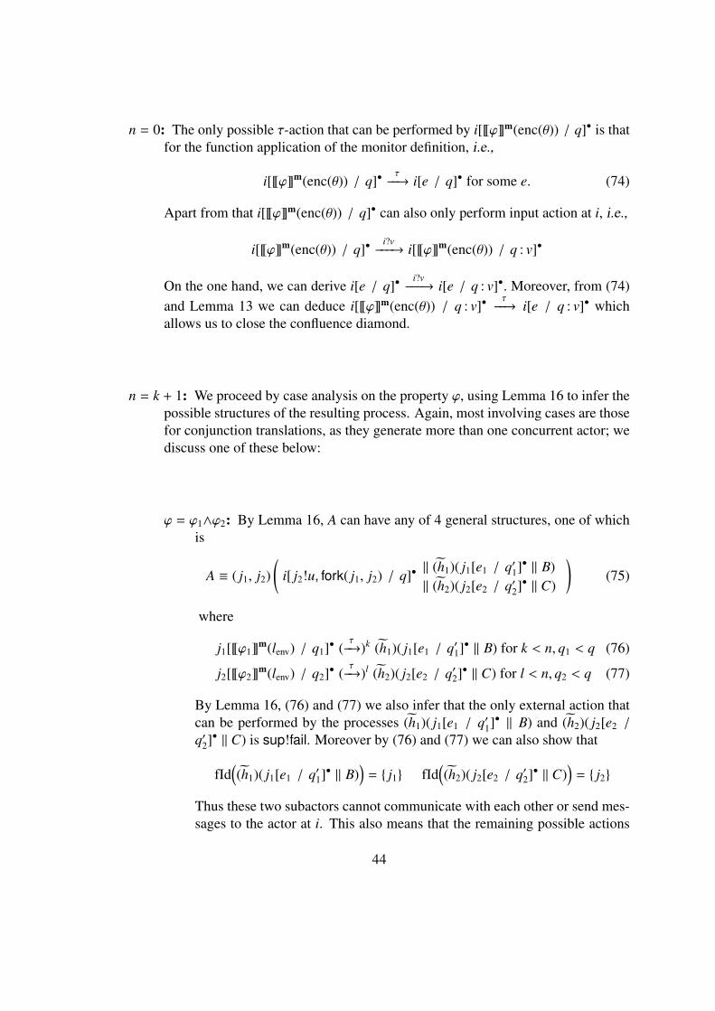
n = 0: The only possible τ-action that can be performed by i[~ϕ�m(enc(θ)) / q]• is thatfor the function application of the monitor definition, i.e.,

i[~ϕ�m(enc(θ)) / q]•τ−−→ i[e / q]• for some e. (74)

Apart from that i[~ϕ�m(enc(θ)) / q]• can also only perform input action at i, i.e.,

i[~ϕ�m(enc(θ)) / q]•i?v−−−→ i[~ϕ�m(enc(θ)) / q : v]•

On the one hand, we can derive i[e / q]•i?v−−−→ i[e / q : v]•. Moreover, from (74)

and Lemma 13 we can deduce i[~ϕ�m(enc(θ)) / q : v]•τ−−→ i[e / q : v]• which

allows us to close the confluence diamond.

n = k + 1: We proceed by case analysis on the property ϕ, using Lemma 16 to infer thepossible structures of the resulting process. Again, most involving cases are thosefor conjunction translations, as they generate more than one concurrent actor; wediscuss one of these below:

ϕ = ϕ1∧ϕ2: By Lemma 16, A can have any of 4 general structures, one of whichis

A ≡ ( j1, j2)(

i[ j2!u, fork( j1, j2) / q]•‖ (h1)( j1[e1 / q′1]• ‖ B)‖ (h2)( j2[e2 / q′2]• ‖ C)

)(75)

where

j1[~ϕ1�m(lenv) / q1]• (

τ−→)k (h1)( j1[e1 / q′1]• ‖ B) for k < n, q1 < q (76)

j2[~ϕ2�m(lenv) / q2]• (

τ−→)l (h2)( j2[e2 / q′2]• ‖ C) for l < n, q2 < q (77)

By Lemma 16, (76) and (77) we also infer that the only external action thatcan be performed by the processes (h1)( j1[e1 / q′1]• ‖ B) and (h2)( j2[e2 /q′2]• ‖ C) is sup!fail. Moreover by (76) and (77) we can also show that

fId((h1)( j1[e1 / q′1]• ‖ B)

)= { j1} fId

((h2)( j2[e2 / q′2]• ‖ C)

)= { j2}

Thus these two subactors cannot communicate with each other or send mes-sages to the actor at i. This also means that the remaining possible actions

44

that A can perform are:

Aτ−−→ ( j1, j2)

(i[u, fork( j1, j2) / q]•

‖ (h1)( j1[e1 / q′1]• ‖ B)‖ (h2)( j2[e2 / q′2 : u]• ‖ C)

)(78)

Aτ−−→ ( j1, j2)

(i[ j2!u, fork( j1, j2) / q]•

‖ (h′1)( j1[e′1 / q′′1 ]• ‖ B′)‖ (h2)( j2[e2 / q′2]• ‖ C)

)because

(h1)( j1[e1 / q′1]• ‖ B)τ−−→ ( h′1 )( j1[e′1 / q′′1 ]• ‖ B′)

(79)

Aτ−−→ ( j1, j2)

(i[ j2!u, fork( j1, j2) / q]•

‖ (h1)( j1[e1 / q′1]• ‖ B)‖ (h′2)( j2[e′2 / q′′2 ]• ‖ C′)

)because

(h2)( j2[e2 / q′2]• ‖ C)τ−−→ ( h′2 )( j2[e′2 / q′′2 ]• ‖ C′)

(80)

Ai?v−−−→ ( j1, j2)

i[ j2!u, fork( j1, j2) / q : v]•

‖ (h1)( j1[e1 / q′1]• ‖ B)‖ (h2)( j2[e2 / q′2]• ‖ C)

(81)

We consider actions (78) and (80) and leave the other combinations for theinterested reader. From (80) and Lemma 13 we derive

(h2)( j2[e2 / q′2 : u]• ‖ C)τ−−→ ( h′2 )( j2[e′2 / q′′2 : u]• ‖ C′)

and by Par and Scp we obtain

( j1, j2)(

i[u, fork( j1, j2) / q]•‖ (h1)( j1[e1 / q′1]• ‖ B)‖ (h2)( j2[e2 / q′2 : u]• ‖ C)

)τ−−→

( j1, j2)(

i[u, fork( j1, j2) / q]•‖ (h1)( j1[e1 / q′1]• ‖ B)‖ (h′2)( j2[e′2 / q′′2 : u]• ‖ C′)

)(82)

45

Using Com, Str, Par and Scp we can derive

( j1, j2)(

i[ j2!u, fork( j1, j2) / q]•‖ (h1)( j1[e1 / q′1]• ‖ B)‖ (h′2)( j2[e′2 / q′′2 ]• ‖ C′)

)τ−−→

( j1, j2)(

i[u, fork( j1, j2) / q]•‖ (h1)( j1[e1 / q′1]• ‖ B)‖ (h′2)( j2[e′2 / q′′2 : u]• ‖ C′)

)(83)

thus we close the confluence diamond by (82) and (83). �

Lemma 18 (Weak Confluence) For all ϕ ∈ sHML, q ∈ Val∗

imon[M(ϕ) / q]∗ ===⇒ A implies cnf(A)

Proof By strong induction on n, the number of reduction steps imon[M(ϕ) / q]∗ (τ−−→)n A.

n = 0 We know A = imon[M(ϕ) / q]∗. It is confluent because it can perform either oftwo actions, namely a τ-action for the function application (see App in Figure 3),or else an external input at imon, (see RcvU in Fig 2). The matching moves can beconstructed by RcvU on the one hand, and by Lemma 13 on the other, analogouslyto the base case of Lemma 17.

n = k + 1 By performing a similar analysis to that of Lemma 16, but for imon[M(ϕ) /q]∗, we can determine that this actor can only weakly transition to either of thefollowing forms:

1. A = imon[M = spw (~ϕ�m(nil)), mLoop(M) / q]∗

2. A ≡ (i)(imon[mLoop(i) / q]∗ ‖ B

)where i[~ϕ�m(lenv) / r]• =⇒ B for

some r.

3. A ≡ (i)(imon[rcv z→ i!z end, mLoop(i) / q]∗ ‖ B

)where

i[~ϕ�m(lenv) / r]• =⇒ B for some r.

4. A ≡ (i)(imon[i!v, mLoop(i) / q]∗ ‖ B


some r.

5. A ≡ (i)(imon[v, mLoop(i) / q]∗ ‖ B


some r.

We here focus on the 4th case of monitor structure; the other cases are analogous.From i[~ϕ�m(lenv) / r]• =⇒ B and Lemma 16 we know that

Bγ−−→ implies γ = sup!fail or γ = τ

B ≡ (~h)(i[e / r]• ‖ C

)where fId(B) = i

46

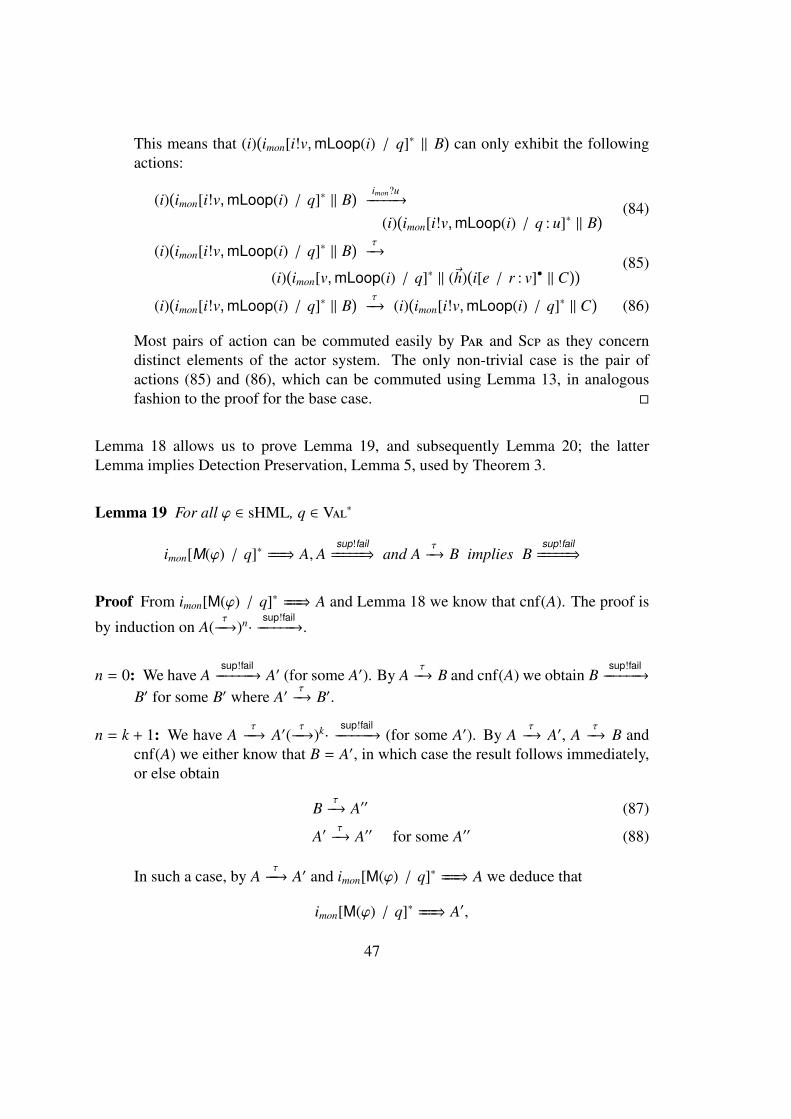
This means that (i)(imon[i!v, mLoop(i) / q]∗ ‖ B

)can only exhibit the following

actions:

(i)(imon[i!v, mLoop(i) / q]∗ ‖ B

) imon?u−−−−−→

(i)(imon[i!v, mLoop(i) / q : u]∗ ‖ B

) (84)


) τ−→

(i)(imon[v, mLoop(i) / q]∗ ‖ (~h)

(i[e / r : v]• ‖ C

)) (85)


) τ−→ (i)

(imon[i!v, mLoop(i) / q]∗ ‖ C

)(86)

Most pairs of action can be commuted easily by Par and Scp as they concerndistinct elements of the actor system. The only non-trivial case is the pair ofactions (85) and (86), which can be commuted using Lemma 13, in analogousfashion to the proof for the base case. �

Lemma 18 allows us to prove Lemma 19, and subsequently Lemma 20; the latterLemma implies Detection Preservation, Lemma 5, used by Theorem 3.

Lemma 19 For all ϕ ∈ sHML, q ∈ Val∗

imon[M(ϕ) / q]∗ ===⇒ A, Asup!fail

=====⇒ and Aτ−→ B implies B

sup!fail=====⇒

Proof From imon[M(ϕ) / q]∗ ===⇒ A and Lemma 18 we know that cnf(A). The proof is

by induction on A(τ−−→)n·

sup!fail−−−−−−→.

n = 0: We have Asup!fail−−−−−−→ A′ (for some A′). By A

τ−→ B and cnf(A) we obtain B


B′ for some B′ where A′τ−→ B′.

n = k + 1: We have Aτ−−→ A′(

τ−−→)k·

sup!fail−−−−−−→ (for some A′). By A

τ−→ A′, A

τ−→ B and

cnf(A) we either know that B = A′, in which case the result follows immediately,or else obtain

Bτ−→ A′′ (87)

A′τ−→ A′′ for some A′′ (88)

In such a case, by Aτ−−→ A′ and imon[M(ϕ) / q]∗ ===⇒ A we deduce that

imon[M(ϕ) / q]∗ ===⇒ A′,

47

and subsequently, by (88), A′(τ−−→)k·

sup!fail−−−−−−→ and I.H. we obtain A′′

sup!fail=====⇒; the

required result then follows from (87). �

Lemma 20 (Detection Confluence) For all ϕ ∈ sHML, q ∈ Val∗

imon[M(ϕ) / q]∗ ===⇒ A, Asup!fail

=====⇒ and A ===⇒ B implies Bsup!fail

=====⇒

Proof By induction on A(τ−−→)nB:

n = 0: The result is immediate since B = A.

n = k + 1: For some B′, We have Aτ−→ B′ and B′(

τ−→)kB. From A

τ−→ B′, A

sup!fail=====⇒,

imon[M(ϕ) / q]∗ ===⇒ A and Lemma 19 we obtain

B′sup!fail

=====⇒ . (89)

By imon[M(ϕ) / q]∗ ===⇒ A and Aτ−→ B′ we obtain imon[M(ϕ) / q]∗ ===⇒ B′ and by

B′(τ−→)kB, (89) and I.H. we obtain B

sup!fail=====⇒. �

Recall Lemma 5 (Detection Preservation). For all ϕ ∈ sHML, q ∈ Val∗

imon[M(ϕ) / q]∗sup!fail

=====⇒ and imon[M(ϕ) / q]∗ ===⇒ B implies Bsup!fail

=====⇒

Proof Immediate, by Lemma 20 for the special case where imon[M(ϕ) / q]∗ ===⇒ imon[M(ϕ) /q]∗. �

6.1.3 Monitor Separability

With the body of supporting lemmata proved thus far, the proof for Lemma 6 turns outto be relatively straightforward. In particular, we make use of Lemma 3, relating thebehaviour of a monitored system to the same system when unmonitored, Lemma 13delineating behaviour preservation after extending mailbox contents at specific actors,and Lemma 16, so as to reason about the structure and generic behaviour of synthesisedmonitors.

48

Recall Lemma 6 (Monitor Separability). For all basic actors ϕ ∈ sHML, A ∈ Actrwhere imon is fresh to A, and s ∈ Act∗ \ {sup!fail},


) s=⇒ B implies ∃B′, B′′s.t.

B ≡ (imon)

(B′ ‖ B′′

)A

s==⇒ A′ s.t. B′ = dA′e

imon[M(ϕ) / tr(s)]∗ ==⇒ B′′

Proof By induction on n in (imon)(dAe ‖ imon[M(ϕ)]∗

)(

γk−−→ )nB, the length of the se-

quence of actions:

n = 0: We know that s = ε and A = (imon)(dAe ‖ imon[M(ϕ)]∗

). Thus the conditions hold

trivially.

n = k + 1: We have (imon)(dAe ‖ imon[M(ϕ)]∗

)(

γk−−→ )kC

γ−−→ B. By I.H. we know that

C ≡ (imon)(C′ ‖ C′′

)(90)

At

==⇒ A′′ s.t. C′ = dA′′e (91)imon[M(ϕ) / tr(t)]∗ ==⇒ C′′ (92)γ = τ implies t = s and γ = α implies tα = s (93)

and by (92) and Lemma 16 we know that

C′′ ≡ (~h)(imon[e / q]∗ ‖ C′′′

)(94)

fId(C′′) = {imon} (95)

We proceed by considering the two possible subcases for the structure of γ:

γ = α: By (93) we know that s = tα. By (95) and (94), it must be the case thatC ≡ (imon)

(C′ ‖ C′′

) α−−→ B happens because

for some B′ C′α−−→ B′ (96)

B ≡ (imon)(B′ ‖ (~h)

(imon[e / q : tr(α)]∗ ‖ C′′′

))(97)

By (96), (91) and Lemma 3 we know that ∃A′ such that dA′e = B′ and thatA′′

α−−→ A′. Thus by (91) and s = tα we obtain

As

==⇒ A′ s.t. B′ = dA′e

49

By (92), (94) and repeated applications of Lemma 13 we also know that

imon[M(ϕ) / tr(t) : tr(α)]∗ = imon[M(ϕ) / tr(s)]∗ ==⇒

(~h)(imon[e / q : tr(α)]∗ ‖ C′′′

)= B′′

The result then follows from (97).

γ = τ: Analogous to the other case, where we also have the case that the reductionis instigated by C′′, in which case the results follows immediately. �

7 Related Work

Runtime monitoring of web services and component-based systems has attracted a con-siderable amount of study, e.g., [FJN+11, GCN+07, CPQFC10] focussing on verifyingsystems with respect to external interactions with clients of the services or components.The type of correctness properties that this body of work describes is similar to theproperties that can be specified using sHML formulas involving external interactions.These systems are generally based on the design by contract principle and RV is appliedto verify whether such systems are satisfying the contract they were designed to satisfy.To the best of our knowledge, none of the works in this area tackles aspects of correctmonitor synthesis but only focus their evaluation on performance benchmarks.

Colombo et al. [CFG11, CFG12] present an RV tool, eLarva, that also makes use of thetracing mechanism in Erlang to gather the execution trace of the system. In eLarva, aspecification of an automata is synthesised into an Erlang program. Several other worksand tools such as MOP [CR03, CR07], Larva [CPS09] and polyLarva [CFMP12] im-plement the monitors using an aspect-oriented programming approach by synthesisingmonitors as aspects that are weaved at runtime with the system under test. The con-currency aspect in these tools is hidden within the AOP library being used, in mostcases AspectJ. Thus, the correctness of the tool also depends on how concurrency iswell-handled in such AOP tools. In these works, the authors do not tackle the issue ofcorrectly synthesising the specification i.e., the correctness of the translation betweenthe specification of the property to the concrete monitor.

The works of Geilen [Gei01] and Sen [SRA04] focus on monitor correctness for LTLformulas defined over infinite strings and give their synthesis in terms of automata andpseudo-code resp.. Leuker et al. [BLS11] also present a translation from LTL to non-deterministic Buchi automata that recognizes good and bad prefixes and as a result actsas monitors for a specified LTL formula. The monitor specifications however sit at ahigher level of abstraction than ours, e.g., Buchi automata, and avoids issues relating toconcurrent monitoring.

50

Fredlund [Fre01] adapted the µ-calculus, which is a variant of HML with recursion, tospecify correctness properties in Erlang albeit for model-checking purposes. Fredlundalso gives a formal semantics for Erlang but does not provide a monitoring semanticsfor the tracing functionality available in the EVM.

Finally, there is work that gives translation of HML with recursion formulas to tests ina process calculus such as CCS [Mil82]. Aceto et al. [AI99] gives such a translation,restricting it to a subset of the HML with recursion for safety properties, similar to thelogic discussed in Section 3. Cerone and Hennessy [CH10] built on this and differen-tiate between may and must testing. None of the synthesised CCS tests are concurrenthowever; we have also already discussed how tests differ from monitors in Section 4.

8 Conclusions

We have studied the problem of ensuring monitor correctness in concurrent settings. Inparticular, we have constructed a formally-specified tool that automatically synthesisesmonitors from sHML formulas so as to asynchronously detect property violation byErlang programs at runtime. We have then showed how the synthesised monitors can beproven correct with respect to a novel definition for monitor correctness in concurrentsettings.

The contributions of the paper are:

1. We present a monitoring semantics for a core subset of Erlang, Figures 2, 3, 4and 5, modelling the tracing mechanism offered by the Erlang VM, and used byasynchronous monitoring tools such as the one presented in this paper and byothers, such as Exago [DWA+10] and eLarva [CFG11, CFG12].

2. We adapt sHML to be able to specify safety Erlang properties, Def. 4. We give analternative, violation characterisation for sHML, Def. 5, that is more amenable toreasoning about violating executions of concurrent (Erlang) programs. We provethat this violation relation corresponds to the dual of the satisfaction definition ofthe same logic, Theorem 1, and also prove that sHML is indeed a safety language,Theorem 2, in the sense of [MP90, CMP92].

3. We give a formal translation form sHML formulas to Erlang expressions fromwhich we construct a tool, available at [Sey13], that allows us to automate concurrent-monitor synthesis.

4. We formalise a novel definition of monitor correctness in concurrent settings,Def. 11, dealing with issues such as non-determinism and divergence.

51

5. We propose a proof technique that teases apart different aspects of the monitorcorrectness definition, Lemma 4, Lemma 5 and Lemma 6, allowing us to provecorrectness in stages. We subsequently apply this technique to prove that oursynthesised monitors are correct, Theorem 3.

Future Work There are many avenues emanating from this work that are worth in-vestigating. The Erlang monitoring semantics of Section 2 can be used as a basis toformally prove existing Erlang monitoring tools such as [CFG11, CFG12]. There isalso substantial work to be done on logics for runtime verification; a simple examplewould be extending sHML to handle limited, monitorable forms of liveness properties(often termed co-safety properties [MP90, CMP92]). It is also worth exploring mecha-nisms for synchronous monitoring, as opposed to asynchronous variant studied in thispaper.

The overheads of the monitors produced by our synthesis need to be assessed better.We also conjecture that more efficient monitor synthesis, perhaps using Erlang featuressuch as process linking and supervision, can be attained; our framework can probablybe extended in straightforward fashion to reason about the correctness of these moreefficient monitors.

Monitor distribution can also be used to lower monitoring overheads even further [CFMP12]and Erlang provides the necessary abstractions to facilitate distribution. Distributedmonitoring can also be used to increase the expressivity of our tool so as to handlecorrectness properties for distributed programs. The latter extension, however, poses adeparture from our setting because the unique trace described by our framework wouldbe replaced by separate independent traces at each location, and the lack of a total or-dering of events may prohibit the detection of certain violations [FGP11, FGP12].

There is also substantial work to be done on how to handle the violations detected,which changes the focus from runtime verification to runtime enforcement [FFM12]. Inthe case of Erlang, corrective actions may range from the complete halting of the sys-tem, to more surgical halting of the violating actors (through exit-killing and trappingmechanism[Arm07, CT09]), to the runtime replacement of the violating sub-systemwith “limp-home” code that provides limited functionality known (a-priori) to be safe;the latter violation handling mechanisms allow for a more pragmatic, graceful degrada-tion of the system being analysed.

52

References

[AI99] Luca Aceto and Anna Ingolfsdottir. Testing Hennessy-Milner Logic withRecursion. In Proceedings of the Second International Conference onFoundations of Software Science and Computation Structure, Held as Partof the European Joint Conferences on the Theory and Practice of Software,ETAPS’99, FoSSaCS ’99, pages 41–55, London, UK, 1999. Springer-Verlag.

[Arm07] Joe Armstrong. Programming Erlang - Software for a Concurrent World.The Pragmatic Bookshelf, 2007.

[BFF+10] Howard Barringer, Ylies Falcone, Bernd Finkbeiner, Klaus Havelund, In-sup Lee, Gordon J. Pace, Grigore Rosu, Oleg Sokolsky, and Nikolai Till-mann, editors. First International Conference, RV 2010, volume 6418 ofLecture Notes in Computer Science. Springer, 2010.

[BLS11] Andreas Bauer, Martin Leucker, and Christian Schallhart. Runtime verifi-cation for ltl and tltl. ACM Trans. Softw. Eng. Methodol., 20:14:1–14:64,September 2011.

[Car01] Richard Carlsson. An introduction to core erlang. In PLI01 (Erlang Work-shop), 2001.

[CFG11] Christian Colombo, Adrian Francalanza, and Rudolph Gatt. Elarva: Amonitoring tool for erlang. In Sarfraz Khurshid and Koushik Sen, editors,Runtime Verification, volume 7186 of Lecture Notes in Computer Science,pages 370–374. Springer Berlin Heidelberg, 2011.

[CFG12] Christian Colombo, Adrian Francalanza, and Ian Grima. Simplifyingcontract-violating traces. In Proceedings Sixth Workshop on Formal Lan-guages and Analysis of Contract-Oriented Software, volume 94 of EPTCS,pages 11–20, 2012.

[CFMP12] Christian Colombo, Adrian Francalanza, Ruth Mizzi, and Gordon J. Pace.polylarva: Runtime verification with configurable resource-aware moni-toring boundaries. In SEFM, pages 218–232, 2012.

[CH10] Andrea Cerone and Matthew Hennessy. Process behaviour: Formulae vs.tests (extended abstract). In EXPRESS’10, pages 31–45, 2010.

[CMP92] Edward Chang, Zohar Manna, and Amir Pnueli. Characterization of tem-poral property classes. In In Proc. Automata, Languages and Program-ming, volume 623 of LNCS, pages 474–486. Springer-Verlag, 1992.

53

[CPQFC10] Tien-Dung Cao, Trung-Tien Phan-Quang, P. Felix, and R. Castanet. Au-tomated runtime verification for web services. In Web Services (ICWS),2010 IEEE International Conference on, pages 76 –82, july 2010.

[CPS09] C. Colombo, G.J. Pace, and G. Schneider. Larva — safer monitoring ofreal-time java programs (tool paper). In Software Engineering and FormalMethods, 2009 Seventh IEEE International Conference on, pages 33 –37,nov. 2009.

[CR03] Feng Chen and Grigore Rosu. Towards monitoring-oriented programming:A paradigm combining specification and implementation. In ElectronicNotes in Theoretical Computer Science, pages 106–125. Elsevier Science,2003.

[CR07] Feng Chen and Grigore Rosu. Mop: An efficient and generic runtimeverification framework. Technical Report UIUCDCS-R-2007-2836, Uni-versity of Illinois at Urbana-Champaign, March 2007.

[CT09] Francesco Cesarini and Simon Thompson. ERLANG Programming.O’Reilly, 2009.

[DWA+10] John Derrick, Neil Walkinshaw, Thomas Arts, Clara Benac Earle,Francesco Cesarini, Lars-Ake Fredlund, Victor Gulias, John Hughes, andSimon Thompson. Property-based testing - the protest project. In FrankS.Boer, MarcelloM. Bonsangue, Stefan Hallerstede, and Michael Leuschel,editors, Formal Methods for Components and Objects, volume 6286 ofLecture Notes in Computer Science, pages 250–271. Springer Berlin Hei-delberg, 2010.

[FFM12] Ylies Falcone, Jean-Claude Fernandez, and Laurent Mounier. What canyou verify and enforce at runtime? STTT, 14(3):349–382, 2012.

[FGP11] Adrian Francalanza, Andrew Gauci, and Gordon J. Pace. Distributed sys-tem contract monitoring. In FLACOS, volume 68 of EPTCS, pages 23–37,2011.

[FGP12] Adrian Francalanza, Andrew Gauci, and Gordon Pace.Distributed system contract monitoring. Accessible athttp://staff.um.edu.mt/afra1/papers/mon-framewk.pdf

(submitted for publication), 2012.

[FJN+11] Ylies Falcone, Mohamad Jaber, Thanh-Hung Nguyen, Marius Bozga, andSaddek Bensalem. Runtime verification of component-based systems. In

54

Software Engineering and Formal Methods (SEFM), volume 7041 of Lec-ture Notes in Computer Science, pages 204–220. Springer, 2011.

[Fre01] Lars-Åke Fredlund. A Framework for Reasoning about Erlang Code. PhDthesis, Royal Institute of Technology, Stockholm, Sweden, 2001.

[GCN+07] Yuan Gan, Marsha Chechik, Shiva Nejati, Jon Bennett, Bill O’Farrell, andJulie Waterhouse. Runtime monitoring of web service conversations. InProceedings of the 2007 conference of the center for advanced studies onCollaborative research, CASCON ’07, pages 42–57, Riverton, NJ, USA,2007. IBM Corp.

[Gei01] Marc Geilen. On the construction of monitors for temporal logic proper-ties. ENTCS, 55(2):181–199, 2001.

[HBS73] Carl Hewitt, Peter Bishop, and Richard Steiger. A universal modular actorformalism for artificial intelligence. In IJCAI, pages 235–245. MorganKaufmann, 1973.

[HM85] Matthew Hennessy and Robin Milner. Algebraic laws for nondeterminismand concurrency. J. ACM, 32(1):137–161, January 1985.

[Koz83] Dexter Kozen. Results on the propositional µ-calculus. Theor. Comput.Sci., 27:333–354, 1983.

[KVK+04] MoonZoo Kim, Mahesh Viswanathan, Sampath Kannan, Insup Lee, andOleg Sokolsky. Java-mac: A run-time assurance approach for java pro-grams. Formal Methods in System Design, 24:129–155, 2004.

[Mil82] R. Milner. A Calculus of Communicating Systems. Springer-Verlag NewYork, Inc., Secaucus, NJ, USA, 1982.

[Mil89] R. Milner. Communication and concurrency. Prentice-Hall, Inc., UpperSaddle River, NJ, USA, 1989.

[MJG+11] Patrick O’Neil Meredith, Dongyun Jin, Dennis Griffith, Feng Chen, andGrigore Rosu. An overview of the MOP runtime verification framework.International Journal on Software Techniques for Technology Transfer,2011. To appear.

[MP90] Zohar Manna and Amir Pnueli. A hierarchy of temporal properties (in-vited paper, 1989). In Proceedings of the ninth annual ACM symposiumon Principles of distributed computing, PODC ’90, pages 377–410, NewYork, NY, USA, 1990. ACM.

55

[MPW93] Robin Milner, Joachim Parrow, and David Walker. Modal logics for mo-bile processes. Theoretical Computer Science, 114:149–171, 1993.

[RV07] Arend Rensink and Walter Vogler. Fair testing. Inf. Comput., 205(2):125–198, February 2007.

[Sey13] Aldrin Seychell. DetectEr, 2013. Accessible athttp://www.cs.um.edu.mt/svrg/Tools/detectEr/.

[SFBE10] Hans Svensson, Lars-Åke Fredlund, and Clara Benac Earle. A unifiedsemantics for future erlang. In Proceedings of the 9th ACM SIGPLANworkshop on Erlang, Erlang ’10, pages 23–32, New York, NY, USA, 2010.ACM.

[SRA04] Koushik Sen, Grigore Rosu, and Gul Agha. Generating optimal lineartemporal logic monitors by coinduction. In ASIAN, volume 2896 of LNCS,pages 260–275. Springer-Verlag, 2004.

[SVAR04] Koushik Sen, Abhay Vardhan, Gul Agha, and Grigore Rosu. Efficientdecentralized monitoring of safety in distributed systems. InternationalConference on Software Engineering, pages 418–427, 2004.

9 Appendix

Definition 14 We define idv, ide and idg as follows:

idv(v)def=

{i} if v = iidv(u) if v = µy.λx.uide(e) if v = µy.λx.e⋃n

i=0 idv(ui) if v = {u0, . . . un}

idv(u) ∪ idv(l) if v = u : l∅ if v = a or x or nil or exit

ide(e)def=

ide(d) if e = spw dide(e′) ∪ ide(d) if e = e′!d or try e′ catch d or x = e′, d or e′(d)idg(g) if e = rcv g endide(d) ∪ idg(g) if e = case d of g end∅ if e = self or x or nil or exit

idg(g)def=

ide(e) ∪ idg( f ) if g = p→ e ; f∅ if g = ε

56

Synthesising Correct Concurrent Runtime Monitors in Erlangsvrg/Papers/shml-correct.pdf ·...

Documents

Transcript of Synthesising Correct Concurrent Runtime Monitors in Erlangsvrg/Papers/shml-correct.pdf ·...