Synthesis of Timing Parameters SatisfyingSafety Properties

Etienne Andre and Romain Soulat

LSV, ENS Cachan & CNRS

Abstract. Safety properties are crucial when verifying real-time con-current systems. When reasoning parametrically, i.e., with unknown con-stants, it is of high interest to infer a set of parameter valuations consis-tent with such safety properties. We present here algorithms based on theinverse method for parametric timed automata: given a reference param-eter valuation, it infers a constraint such that, for any valuation satisfyingthis constraint, the discrete behavior of the system is the same as underthe reference valuation in terms of traces, i.e., alternating sequences oflocations and actions. These algorithms do not guarantee the equalityof the trace sets, but are significantly quicker, synthesize larger sets ofparameter valuations than the original method, and still preserve vari-ous properties including safety (i.e., non-reachability) properties. Thosealgorithms have been implemented in Imitator II and applied to variousexamples of asynchronous circuits and communication protocols.

Keywords: Real-Time Systems, Timed Automata, Verification, Imitator

1 Introduction

Timed Automata are finite-state automata augmented with clocks, i.e., real-valued variables increasing uniformly, that are compared within guards and tran-sitions with timing delays [AD94]. Although techniques can be used in order toverify the correctness of a timed automaton for a given set of timing delays, thesetechniques become inefficient when verifying the system for a large number ofsets of timing delays, and don’t apply anymore when one wants to verify denseintervals of values, or optimize some of these delays. It is therefore interesting toreason parametrically, by assuming that those timing delays are unknown con-stants, or parameters, which give Parametric Timed Automata (PTAs) [AHV93].

We consider here the good parameters problem [FJK08]: “given a PTA Aand a rectangular domain V bounding the value of each parameter, find all theparameter valuations within V such that A has a good behavior”. Such goodbehaviors can refer to any kind of properties. We will in particular focus here onsafety properties, i.e., the non-reachability of a given set of “bad” locations.

Parameters Synthesis for PTAs. The problem of parameter synthesis is knownto be undecidable for PTAs, although semi-algorithms exist [AHV93] (i.e., ifthe algorithm terminates, the result is correct). The synthesis of constraints hasbeen implemented in the context of PTAs or hybrid systems, e.g., in [AAB00]using TReX [CS01], or in [HRSV02] using an extension of Uppaal [LPY97] forlinear parametric model checking. In [HRSV02], decidability results are givenfor a subclass of PTAs, viz., “L/U automata”.

The problem of parameter synthesis for timed automata has been applied inparticular to communication protocols (e.g., the Bounded Retransmission Proto-col [DKRT97] using Uppaal and Spin [Hol03], and the Root Contention Protocolin [CS01] using TReX) and asynchronous circuits (see, e.g., [YKM02,CC07]).

The authors of [KP10] synthesize a set of parameter valuations under which agiven property specified in the existential part of CTL without the next operator(ECTL−X) holds in a system modeled by a network of PTAs. This is done byusing bounded model checking techniques applied to PTAs.

In the framework of Linear Hybrid Automata, techniques based on counterex-ample guided abstraction refinement (CEGAR) [CGJ+00] have been proposed.In [JKWC07], a method of iterative relaxation abstraction is proposed, com-bining CEGAR and linear programming. In [FJK08], when finding a counterex-ample, the system obtains constraints that make the counterexample infeasible.When all the counterexamples have been eliminated, the resulting constraintsdescribe a set of parameters for which the system is safe. Also note that anapproach similar to the inverse method is proposed in [AKRS08], in order tosynthesize initial values for the variables of a linear hybrid system.

Contribution. We introduced in [ACEF09] the inverse method IM for PTAs.Different from CEGAR-based methods, this original semi-algorithm for param-eter synthesis is based on a “good” parameter valuation π0 instead of a set of“bad” states. IM synthesizes a constraint K0 on the parameters such that, forall parameter valuation π satisfying K0, the trace set, i.e., the discrete behav-ior, of A under π is the same as for A under π0. This preserves in particularlinear time properties. However, this equality of trace sets may be seen as a toostrong property in practice. Indeed, one is rarely interested in a strict orderingof the events, but rather in the partial match with the original trace set, or moregenerally in the non-reachability of a given set of bad locations.

We present here several algorithms based on IM , which do not preserve theequality of trace sets, but preserve various properties. In particular, they allpreserve non-reachability: if a location is not reachable in A under π0, it will notbe reachable in A under π, for π satisfying K0. The main advantage is that thesealgorithms synthesize weaker constraints, i.e., larger sets of parameters. Beside,termination is improved when compared to the original IM and the computationtime is reduced, as shown in practice in the implementation Imitator II.

Plan of the Paper. We briefly recall IM in Section 2. We introduce in Section 3algorithms based on IM synthesizing weaker constraints for safety properties,

and show their interest compared to IM . We extend in Section 4 these algo-rithms in order to perform a behavioral cartography of the system. We show inSection 5 the interest in practice by applying these algorithms to models of theliterature. We also introduce algorithmic optimizations for two variants allowingto considerably reduce the state space. We conclude in Section 6.

2 The Inverse Method

Preliminaries. 1 Given a setX of clocks and a set P of parameters, a constraint Cover X and P is a conjunction of linear inequalities on X and P . Given aparameter valuation (or point) π, we write π |= C when the constraint where allparameters within C have been replaced by their value as in π is satisfied by anon-empty set of clock valuations. We denote by ∃X : C the constraint over Pobtained from C after elimination of the clocks in X.

Definition 1. A PTA A is (Σ,Q, q0, X, P,K, I,→) with Σ a finite set of ac-tions, Q a finite set of locations, q0 ∈ Q the initial location, X a set of clocks, Pa set of parameters, K a constraint over P , I the invariant assigning to everyq ∈ Q a constraint over X and P , and → a step relation consisting of elements(q, g, a, ρ, q′), where q, q′ ∈ Q, a ∈ Σ, ρ ⊆ X is the set of clocks to be reset, andthe guard g is a constraint over X and P .

The semantics of a PTA A is defined in terms of states, i.e., couples (q, C)where q ∈ Q and C is a constraint over X and P . Given a point π, we saythat a state (q, C) is π-compatible if π |= C. Runs are alternating sequences ofstates and actions, and traces are time-abstract runs, i.e., alternating sequencesof locations and actions. The trace set of A corresponds to the traces associatedwith all the runs of A. Given A and π, we denote by A[π] the (non-parametric)timed automaton where each occurrence of a parameter has been replaced by itsconstant value as in π. Given two states s1 = (q1, C1) and s1 = (q2, C2), we saythat s1 is included into s2 if q1 = q2 and C1 ⊆ C2, where ⊆ denotes the inclusionof constraints. One defines Post iA(K)(S) as the set of states reachable from a set S

of states in exactly i steps under K, and Post∗A(K)(S) =⋃

i≥0 Post iA(K)(S).

Description. Given a PTA A and a reference parameter valuation π0, the inversemethod IM synthesizes a constraint K0 on the parameters such that, for allπ |= K0, A[π0] and A[π] have the same trace sets [ACEF09]. We recall IM inAlgorithm 1, which consists in two major steps.

1. The iterative removal of the π0-incompatible states, i.e., states whose con-straint onto the parameters is not satisfied by π0, prevents for any π |= K0

the behavior different from π0 (by negating a π0-incompatible inequality J).2. The final intersection of the projection onto the parameters of the constraints

associated with all the reachable states guarantees that all the behaviorsunder π0 are allowed for all π |= K0.

1 Fully detailed definitions are available in [AS11].

Algorithm 1: Inverse method algorithm IM (A, π0)

input : PTA A of initial state s0, parameter valuation π0

output: Constraint K0 on the parameters

1 i← 0 ; K ← true ; S ← {s0}2 while true do3 while there are π0-incompatible states in S do4 Select a π0-incompatible state (q, C) of S (i.e., s.t. π0 6|= C) ;5 Select a π0-incompatible J in (∃X : C) (i.e., s.t. π0 6|= J) ;

6 K ← K ∧ ¬J ; S ←⋃i

j=0 PostjA(K)({s0}) ;

7 if PostA(K)(S) v S then return⋂

(q,C)∈S(∃X : C)

8 i← i+ 1 ; S ← S ∪ PostA(K)(S) ; // S =⋃i

j=0 PostjA(K)({s0})

Item 1 is compulsory in order to prevent the system to enter “bad” (i.e., π0-incompatible) states. However, item 2 can be lifted when one is only interestedin safety properties. Indeed, in this case, it is acceptable that only part of thebehavior of A[π0] is available in A[π] (as long as the behavior absent from A[π0]is also absent from A[π]).

Properties. The main property of IM is the preservation of trace sets. As aconsequence, linear-time properties are preserved. This is the case of propertiesexpressed using the Linear Time Logics (LTL) [Pnu77], but also using the SE-LTL logics [CCO+04], constituted by both atomic state propositions and events.

It has been shown that IM is non-confluent, i.e., several applications of IMcan lead to different results [And10b]. This comes from the non-deterministicselection of a π0-incompatible inequality J (line 5 in Algorithm 1). IM behavesdeterministically when such a situation of choice is non encountered. The non-confluence of IM leads to the non-maximality of the output constraint. In otherwords, given A and π0, there may exist points π 6|= IM (A, π0) such that A[π]and A[π0] have the same trace sets. However, it can be shown that, when IM isdeterministic, the output constraint is maximal.

Reachability analysis is known to be undecidable for PTAs [AHV93]. Hence,although we showed sufficient conditions, IM does not terminate in general.

3 Optimized Algorithms Based on the Inverse Method

A drawback of IM is that the notion of equality of trace sets may be seen astoo strict in some cases. If one is interested in the non-reachability of a certainset of bad states, then there may exist different trace sets avoiding this set ofbad states. We introduce here several algorithms derived from IM : none of themguarantee the strict equality of trace sets, but all synthesize weaker constraintsthan IM and still feature interesting properties. They all preserve in particularsafety properties, i.e., non-reachability of a given location. In other words, if agiven “bad” location is not reached in A[π0], it will also not be reached by A[π],

for π satisfying the constraint output by the algorithm. The corollary is that theset of locations reachable in A[π] is included into the set reachable in A[π0].

We introduce algorithms derived from IM , namely IM⊆, IM ∪, and IM K .We then introduce combinations between these algorithms. For each algorithm,we briefly state that the constraint is weaker than IM (when applicable), studythe termination, and formally state the properties guaranteed by the outputconstraint. (We do not recall the preservation of non-reachability.) The fullydetailed algorithms and all formal properties with proofs can be found in [AS11].

3.1 Algorithm with State Inclusion in the Fixpoint

The algorithm IM⊆ is obtained from IM by terminating the algorithm, not whenall new states are equal to a state computed previously, but when all new statesare included into a previous state.

The constraint output by IM⊆ is weaker than the one output by IM , andIM⊆ entails an earlier termination than IM for the same input, and hence asmaller memory usage because states are merged as soon as one is included intoanother one. IM⊆ preserves the equality of traces up to length n, where n is thenumber of iterations of IM⊆ (i.e., the depth of the state space exploration).

Proposition 1. Suppose that IM⊆(A, π0) terminates with output K0 after niterations of the outer do loop. Then, we have:

1. π0 |= K0,2. for all π |= K0, for each trace T0 of A[π0], there exists a trace T of A[π] such

that the prefix of length n of T0 and the prefix of length n of T are equal,3. for all π |= K0, for each trace T of A[π], there exists a trace T0 of A[π0] such

that the prefix of length n of T0 and the prefix of length n of T are equal.

Proposition 2. Suppose that IM⊆(A, π0) terminates with output K0. Then, forall π |= K0, the sets of reachable locations of A[π] and A[π0] are the same.

3.2 Algorithm with Union of the Constraints

The algorithm IM ∪ is obtained from IM by returning, not the intersection ofthe constraints associated with all the reachable states, but the union of theconstraints associated with the last state of each run. This notion of last state iseasy to understand for finite runs. When considering infinite (and necessarily2

cyclic) runs, it refers to the second occurrence of a same state within a run, i.e.,the first time that a state is equal to a previous state of the same run.

The constraint output by IM ∪ is weaker than the one output by IM . Notethat the constraints output by IM⊆ and IM ∪ are incomparable (see examplein Section 3.6 for which two incomparable constraints are synthesized). Thetermination is the same as for IM .

2 If the runs are infinite but not cyclic, the algorithm does not terminate.

Although the equality of trace sets is no longer guaranteed for π |=IM ∪(A, π0), we have the guarantee that, for all π |= K0, the trace set of A[π] isa subset of the trace set of A[π0]. Furthermore, each trace of A[π0] is reachablefor at least one valuation π |= K0.

Proposition 3. Let K0 = IM ∪(A, π0). Then:

1. π0 |= K0;2. For all π |= K0, every trace of A[π] is equal to a trace of A[π0];3. For all trace T of A[π0], there exists π |= K0 such that the trace set of A[π]

contains T .

Finally note that, due to the disjunctive form of the returned constraint, thesynthesized constraint is not necessarily convex.

3.3 Algorithm with Direct Return

The algorithm IM K is obtained from IM by returning only the constraint Kcomputed during the algorithm instead of the intersection of the constraintsassociated to all the reachable states.

The constraint output by IM K is weaker than the one output by IM . Alsonote that the constraints output by IM⊆ and IM K are incomparable (see ex-ample in Section 3.6). Termination is the same for IM K and IM .

Proposition 4. Let K0 = IM K(A, π0). Then, for all π |= K0, every traceof A[π] is equal to a trace of A[π0].

This algorithm only prevents π0-incompatible states to be reached but, con-trarily to IM and IM ∪, does not guarantee that any “good” state will be reached.Hence, this algorithm only preserves the non-reachability of locations.

3.4 Combination: Inclusion in Fixpoint and Union

One combine the variant of the fixpoint (viz., IM⊆) with the first variant ofthe constraint output (viz., IM ∪), thus leading to IM ∪

⊆. The constraint out-

put by IM ∪ is weaker than the ones output by both IM⊆ and IM ∪. Note thatthe constraints output by IM ∪

⊆ and IM K are incomparable (see example inSection 3.6 for which two incomparable constraints are synthesized). The termi-nation is the same as for IM⊆. This algorithm combines the properties of IM⊆and IM ∪. Although not of high interest in practice, this result implies preser-vation of non-reachability. Finally note that, due to the disjunctive form of thereturned constraint, the output constraint is not necessarily convex.

3.5 Combination: Inclusion in Fixpoint and Direct Return

One can also combine the variant of the fixpoint (viz., IM⊆) with the secondvariant of the constraint output (viz., IM K), thus leading to IM K

⊆ . The con-

straint output by IM K⊆ is weaker than the ones output by both IM K and IM ∪

⊆.Termination is the same as for IM⊆. This algorithm only preserves the non-reachability of locations.

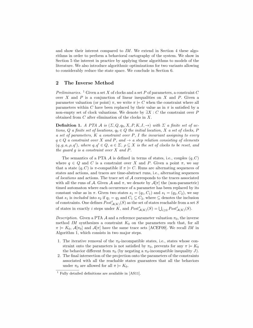
3.6 Summary of the Algorithms

We summarize in Table 1 the properties of each algorithm.

Property IM IM⊆ IM∪ IMK IM∪⊆ IMK⊆

Equality of trace sets√

× × × × ×Equality of trace sets up to n

√ √× × × ×

Inclusion into the trace set of A[π0]√

×√ √

× ×Preservation of at least one trace

√×

√× × ×

Equality of location sets√ √

× × × ×Convex output

√ √×

√×

√

Preservation of non-reachability√ √ √ √ √ √

Table 1. Comparison of the properties of the variants of IM

We give in Figure 1 (left) the relation between terminations: an orientededge from A to B means that, for the same input, termination of variant Aimplies termination of B. We give in Figure 1 (right) the relations between theconstraints synthesized by each variant: for example, given A and π0, we havethat IM (A, π0) ⊆ IM⊆(A, π0). Obviously, the weakest constraint is the onesynthesized by IM K

⊆ . This variant should be thus used when one is interested onlyin safety properties; however, when one is interested in stronger properties (e.g.,preservation of at least one trace of A[π0]), one may want to use another variantaccording to their respective properties. We believe that the most interestingalgorithms are IM , for the equality of trace sets, IM ∪, for the preservation of atleast one maximal trace, and IM K

⊆ , for the sole preservation of non-reachability.

IM IM∪ IMK

IM⊆ IM∪⊆ IMK⊆

IM

IM⊆

IM∪ IMK

IM∪⊆ IMK⊆

⊆

⊆ ⊆

⊆⊆

⊆

⊆

Fig. 1. Comparison of termination (left) and constraint output (right)

Non-maximality. Actually, none of these algorithms synthesize the maximal con-straint corresponding to the property they are characterized with. This is dueto their non-confluence, itself due to the random selection of a π0-incompatibleinequality. However, it can be shown that the constraint is maximal when thealgorithm runs in a fully deterministic way. We address the issue of synthesizinga maximal constraint in Section 4. Also note that the comparison between theconstraints (see Figure 1 (right)) holds only for deterministic analyses.

Comparison Using an Example of PTA. Let us consider the PTA Avar depictedbelow. We consider the following π0: p1 = 1∧p2 = 4. In A[π0], location q4 is notreachable, and can be considered as a “bad” location.

q0 q1 q2

q3

q4

x1 ≤ 2p1∧ x1 ≤ 2 x2 ≤ p2

x1 ≤ p2

ax1 := 0x2 := 0

x1≥ p2c

a

x1≥ 3b

x1 ≥ p1a

x1 := 0

b

c

Fig. 2. A PTA Avar for comparing the variants of IM

Let us suppose that a bad behavior of Avar corresponds to the fact that atrace goes into location q4. Under π0, the system has a good behavior. As aconsequence, by the property of non-reachability of a location met by all algo-rithms, the constraint synthesized by any algorithm also prevents the traces toenter q4. One can show that the parameter valuations allowing the system toenter the bad location q4 are comprised in the domain 2 ∗ p1 ≤ p2 ∧ p2 ≤ 2. Asa consequence, the (non-convex) maximal set of parameters avoiding the badlocation q4 is 2 ∗ p1 > p2 ∨ p2 > 2.

We give below the six constraints synthesized by the six versions of the inversemethod. For each graphics, we depict in dark blue the parameter domain coveredby the constraint, and in light red the parameter domain corresponding to a badbehavior (the constraint itself is given in [AS11]). The “good” zone not coveredby the constraint is depicted in very light gray. The dot represents π0.

This example illustrates well the relationship between the different con-straints. In particular, the constraint synthesized by IM K

⊆ dramatically improvesthe set of parameters synthesized by IM . Also note that we chose on purposean example such that none of the methods synthesizes a maximal constraint(observe that even IM K

⊆ does not cover the whole “good” zone). This will beaddressed in Section 4.

Experimental Validation. The example above shows clearly the gain of the algo-rithms w.r.t. IM . However, for real case studies, although checking the gain ofthese algorithms in terms of computation time is possible, measuring the gain interms of the “size” of the constraints synthesized requires measures of polyhedra,which is not trivial when they are non-convex. Hence, we postpone this studyto the framework of the cartography (see Section 5).

p1

p2

0 1 2 3 4 5 6 7 8

012345678

IM

p1

p2

0 1 2 3 4 5 6 7 8

012345678

IM∪

p1

p2

0 1 2 3 4 5 6 7 8

012345678

IMK

p1

p2

0 1 2 3 4 5 6 7 8

012345678

IM⊆

p1

p2

0 1 2 3 4 5 6 7 8

012345678

IM∪⊆

p1

p2

0 1 2 3 4 5 6 7 8

012345678

IMK⊆

Fig. 3. Comparison of the constraints synthesized for Avar

4 Behavioral Cartography

Although IM has been shown of interest for a large panel of case studies, itsmain shortcoming is the non-maximality of the output constraint. Moreover,the good parameters problem relates to the synthesis of parameter valuationscorresponding to any good behavior, not to a single one.

The behavioral cartography algorithm BC relies on the idea of covering theparameter space within a rectangular real-valued parameter domain V0 [AF10].By iterating IM over all the integer points of V0 (of which there are a finitenumber), one is able to decompose V0 into a list Tiling of tiles, i.e., dense setsof parameters in which the trace sets are the same.

Then, given a property ϕ on trace sets (viz., a linear time property), one canpartition the parameter space between good tiles (for which all points satisfy ϕ)and bad tiles. This can be done by checking the property for one point in eachtile (using, e.g., Uppaal, applied to the PTA instantiated with the consideredpoint). Then the set of parameters satisfying ϕ corresponds to the union of thegood tiles. Note that BC is independent from ϕ; only the partition between goodand bad tiles involves ϕ.

In practice, not only the integer valuations of V0 are covered by Tiling , butalso most of the real-valued space of V0. Furthermore, the space covered by Tilingoften largely exceeds the limits of V0. However, there may exist a finite numberof “small holes” within V0 (containing no integer point) that are not covered byany tile of Tiling . A refinement of BC is to consider a tighter grid, i.e., not onlyinteger points, but rational points multiple of a smaller step than 1. We showedthat, for a rectangle V0 large enough and a grid tight enough, the full coverageof the whole real-valued parameter space (inside and outside V0) is ensured forsome classes of PTAs, in particular for acyclic systems (see [And10b] for details).

Combination with the Variants. By replacing within BC the call to IM by a callto one of the algorithms introduced in Section 3, one changes the properties ofthe tiles: for each tile, the corresponding trace set inherits the properties of theconsidered variant, and does not necessarily preserve the equality of trace sets.However, as shown in Section 3, they all preserve (at least) the non-reachability.

The main advantage of the combination of BC with one of the algorithms,say IM ′, of Section 3 is that the coverage of V0 needs a smaller number of tiles,i.e., of calls to IM ′. Indeed, due to the weaker constraint synthesized by IM ′,and hence larger sets of parameters, one needs less calls to IM ′ in order tocover V0. Furthermore, due to the quicker termination of IM ′ when comparedto IM , the computation time decreases considerably. Finally, due to an earliertermination IM ′ (i.e., less states computed) and the lower number of calls to IM ′

(hence, less trace sets to remember), the memory consumption also decreases.

5 Implementation and Experiments

All these algorithms, as well as the original IM , have been implemented inImitator II [And10a]. We give in Table 2 the summary of various experimentsof parameter synthesis applied to case studies from the literature as well asindustrial case studies. For each case study, we apply each version of BC toa given V0. Then, we split the tiles between good and bad w.r.t. a property.Finally, we synthesize a constraint corresponding to this property. For each casestudy, V0 is either entirely covered, or “almost entirely covered”. We give fromleft to right the name of the case study, the number of parameters varying inthe cartography and the number of points within V0. We then give the numberof tiles and the computation time for each algorithm. We denote by BC⊆ thevariant of BC calling IM⊆ instead of IM (and similarly for the other algorithms).All experiments were performed on an Intel Core 2 Duo 2,33 Ghz with 3,2 Gomemory, using the no-random, no-dot and no-log options of Imitator II.

Example Tiles Time (s)

Name |P | |V0| BC BC∪ BCK BC⊆ BC∪⊆ BCK⊆ BC BC∪ BCK BC⊆ BC∪⊆ BCK

⊆Avar 2 72 14 10 10 7 5 5 0.101 0.079 0.073 0.036 0.028 0.026

Flip-flop 2 644 8 7 7 8 7 7 0.823 0.855 0.696 0.831 0.848 0.699AND–OR 5 151 200 16 14 16 14 14 14 274 7154 105 199 551 68.4

Latch 4 73 062 5 3 3 5 3 3 16.2 25.2 9.2 15.9 25 9.1CSMA/CD 3 2 000 139 57 57 139 57 57 112 276 76.0 46.7 88.0 22.6SPSMALL 2 3 082 272 78 77 272 78 77 894 405 342 894 406 340

Table 2. Comparison of the algorithms for the behavioral cartography

Since V0 is always (at least “almost”) entirely covered by Tiling , the numberof tiles needed to cover V0 gives a measure of the size of each tile in terms ofparameter valuations: the lesser tiles needed, the larger the sets of parametervaluations are, the more efficient the corresponding algorithm is. Since the goodproperty for all case studies is a property of (non-)reachability, the constraint

computed is the same for all versions of BC . The latest version3 of Imitator IIas well as all the mentioned case studies can be found on Imitator II’s Webpage4. Details on case studies can be found in [AS11].

As expected from Section 2, all algorithms bring a significant gain in term ofsize of the constraint, because the number of tiles needed to cover V0 is almostalways smaller than for IM . Only IM⊆ has a number of tiles often equal to IM ;however, the computation is often much quicker for IM⊆. As expected, the mostefficient algorithm is IM K

⊆ : both the number of tiles and the computation timesdecrease significantly. When one is only interested in reachability properties, oneshould then use this algorithm.

The only surprising result is the fact that IM ∪ is sometimes slower than IM ,although the number of tiles is smaller. This is due to the way it is implementedin Imitator II. Handling non-convex constraints is a difficult problem; hence,we compute a list of constraints associated with the last state of each trace.Unfortunately, many of these constraints are actually equal to each other. Forsystems with thousands of traces and hundreds of tiles, we manipulate hundredsof thousands of constraints; every time a new point is picked up, one should checkwhether it belongs to this huge set before calling (or not) IM on this point. Thisalso explains the relatively disappointing speed performance of IM ∪

⊆. Improvingthis implementation is the subject of ongoing work. A possible option would beto remove the constraints equal to each other in this constraint set; this woulddramatically decrease the size of the set, but would induce additional costs forchecking constraint equality.

On-the-fly Computation of K. We finally introduce here another modification ofsome of the algorithms in order to avoid the non-necessary duplication of somereachable states, leading to a dramatic diminution of the state space. Indeed,we met cases where two states (q, C) and (q, C ′) are not equal at the time theyare computed, but are equal with the final intersection K of the constraints, i.e.(q, C∧K) = (q, C ′∧K). Such a situation is depicted in the trace sets of Figure 4,where identical states under IM (A, π0) are unmerged on the left part of thefigure and merged on the right part. We can solve this problem by performingdynamically the intersection of the constraints, i.e., adding ∃X : C to all thestates previously computed, every time a new state (q, C) is computed. This hasthe effect of merging such states, and hence often considerably decreasing thestate space. With this modification, the algorithm only needs to return K at theend of the computation, since the intersection is performed on the fly. We givethis algorithm IM otf in Algorithm 2.

This modification can be extended to IM⊆ in a straightforward manner, byapplying to IM otf the fixpoint modification as described in Section 3.1. However,applying it to other algorithms would modify their correctness, since the finalintersection of the constraints is not performed in the other algorithms.

3 Note that the software named Imitator 3 is an independent fork of Imitator II forhybrid systems [FK11]. The latest version of Imitator for PTAs is Imitator 2.3.

4 http://www.lsv.ens-cachan.fr/Software/imitator/imitator2.3/

Fig. 4. Example of state space explosion due to unmerged states

Algorithm 2: IM otf (A, π0)

input : PTA A of initial state s0, parameter valuation π0

output: Constraint K0 on the parameters

1 i← 0 ; K ← true ; S ← {s0}2 while true do3 foreach s = (q, C) ∈ S do4 if s is π0-incompatible then5 Select a π0-incompatible J in (∃X : C)6 K ← K ∧ ¬J ;7 foreach (q′, C′) ∈ S do8 C′ ← C′ ∧ ¬J

9 else10 K ← K ∧ ∃X : C ;11 foreach (q′, C′) ∈ S do12 C′ ← C′ ∧ ∃X : C

13 if PostA(K)(S) v S then return K

14 i← i+ 1 ; S ← S ∪ PostA(K)(S) ; // S =⋃i

j=0 PostjA(K)({s0})

Using this modification, we successfully computed a set of parameters forthe SPSMALL memory designed by ST-Microelectronics. We analyzed a muchlarger version of the “small” model considered above (see differences betweenthese models in [And10b]). The larger model of this memory contains 28 clocksand 62 parameters. The computation consists in 98 iterations of the outer DOloop of IM . Without this optimization, IM crashed from lack of memory atiteration 27 (on a 2 GB memory machine), but the size of the state space wasexponential, so we believe that the full computation would have required a hugeamount of memory, preventing more powerful machine to perform the compu-tation. Using this optimization, we computed quickly a constraint, made of theconjunction of 49 linear constraints. Full details are available in [And10b].

6 Conclusion

We introduced here several algorithms based on the inverse method for PTAs.Given a PTA A and a reference parameter valuation π0, these algorithms syn-thesize a constraint K0 around π0, all preserving non-reachability properties: if alocation (in general “bad”) is not reached for π0, it is also not reachable for anyπ |= K0. Furthermore, each algorithm preserves different properties: strict equal-ity of trace sets, inclusion within the trace set of A[π0], preservation of at leastone trace of A[π0], etc. The major advantage of these variants is the faster com-putation of K0, and a larger set of parameter valuations defined by K0. Thesealgorithms have been implemented in Imitator II and show significant gains oftime and size of the constraint when compared to the original IM . When used inthe behavioral cartography for synthesizing a constraint w.r.t. a given property,they cover both using less tiles and in general faster the parameter space.

Also recall that, although the algorithms preserve properties based on traces,i.e., untimed behaviors, it is possible to synthesize constraints guaranteeing timedproperties by making use of an observer; this is the case in particular for theSPSMALL memory.

As a future work, the inverse method and the cartography algorithm, as wellas the variants introduced here, could be extended in a rather straightforwardway to the backward case.

Furthermore, we presented in [AFS09] an extension of the inverse method toprobabilistic systems: given a parametric probabilistic timed automaton A anda reference valuation π0, we synthesize a constraint K0 by applying IM to a non-probabilistic version of A and π0. Then, we guarantee that, for all π |= K0, thevalues of the minimum (resp. maximum) probabilities of reachability propertiesare the same in A[π]. Studying what properties each of the algorithms presentedhere preserves in the probabilistic framework is the subject of ongoing work.

It would also be of interest to consider the combination of these algorithmswith the extension of the inverse method to linear hybrid automata [FK11].

References

[AAB00] A. Annichini, E. Asarin, and A. Bouajjani. Symbolic techniques for para-metric reasoning about counter and clock systems. In CAV’00, pages 419–434. Springer-Verlag, 2000.

[ACEF09] E. Andre, T. Chatain, E. Encrenaz, and L. Fribourg. An inverse methodfor parametric timed automata. International Journal of Foundations ofComputer Science, 20(5):819–836, 2009.

[AD94] R. Alur and D.L. Dill. A theory of timed automata. TCS, 126(2):183–235,1994.

[AF10] E. Andre and L. Fribourg. Behavioral cartography of timed automata. InRP’10, volume 6227 of LNCS, pages 76–90. Springer, 2010.

[AFS09] E. Andre, L. Fribourg, and J. Sproston. An extension of the inverse methodto probabilistic timed automata. In AVoCS’09, volume 23 of ElectronicCommunications of the EASST, 2009.

[AHV93] R. Alur, T. A. Henzinger, and M. Y. Vardi. Parametric real-time reasoning.In STOC’93, pages 592–601. ACM, 1993.

[AKRS08] R. Alur, A. Kanade, S. Ramesh, and K. C. Shashidhar. Symbolic analysisfor improving simulation coverage of simulink/stateflow models. In EM-SOFT’08, pages 89–98. ACM, 2008.

[And10a] Etienne Andre. IMITATOR II: A tool for solving the good parametersproblem in timed automata. In INFINITY’10, volume 39 of EPTCS, pages91–99, 2010.

[And10b] Etienne Andre. An Inverse Method for the Synthesis of Timing Param-eters in Concurrent Systems. Ph.d. thesis, Laboratoire Specification etVerification, ENS Cachan, France, 2010.

[AS11] E. Andre and R. Soulat. Synthesis of timing parameters satisfying safetyproperties (full version). Research report, Laboratoire Specification etVerification, ENS Cachan, France, 2011. Available at http://www.lsv.

ens-cachan.fr/Publis/RAPPORTS_LSV/PDF/rr-lsv-2011-13.pdf.[CC07] R. Clariso and J. Cortadella. The octahedron abstract domain. Sci. Comput.

Program., 64(1):115–139, 2007.[CCO+04] S. Chaki, E. M. Clarke, J. Ouaknine, N. Sharygina, and N. Sinha.

State/event-based software model checking. In IFM’04, volume 2999 ofLNCS, pages 128–147. Springer, 2004.

[CGJ+00] E. M. Clarke, O. Grumberg, S. Jha, Y. Lu, and H. Veith. Counterexample-guided abstraction refinement. In CAV’00, pages 154–169. Springer-Verlag,2000.

[CS01] A. Collomb–Annichini and M. Sighireanu. Parameterized reachability anal-ysis of the IEEE 1394 Root Contention Protocol using TReX. In RT-TOOLS’01, 2001.

[DKRT97] P.R. D’Argenio, J.P. Katoen, T.C. Ruys, and G.J. Tretmans. The boundedretransmission protocol must be on time! In TACAS’97. Springer, 1997.

[FJK08] G. Frehse, S.K. Jha, and B.H. Krogh. A counterexample-guided approachto parameter synthesis for linear hybrid automata. In HSCC’08, volume4981 of LNCS, pages 187–200. Springer, 2008.

[FK11] L. Fribourg and U. Kuhne. Parametric verification and test coverage forhybrid automata using the inverse method. In RP’11, volume 6945 of LNCS.Springer, 2011. To appear.

[Hol03] Gerard Holzmann. The Spin model checker: primer and reference manual.Addison-Wesley Professional, 2003.

[HRSV02] T.S. Hune, J.M.T. Romijn, M.I.A. Stoelinga, and F.W. Vaandrager. Lin-ear parametric model checking of timed automata. Journal of Logic andAlgebraic Programming, 2002.

[JKWC07] S.K. Jha, B.H. Krogh, J.E. Weimer, and E.M. Clarke. Reachability forlinear hybrid automata using iterative relaxation abstraction. In HSCC’07,pages 287–300. Springer-Verlag, 2007.

[KP10] M. Knapik and W. Penczek. Bounded model checking for parametric timeautomata. In SUMo’10, 2010.

[LPY97] K.G. Larsen, P. Pettersson, and W. Yi. Uppaal in a nutshell. InternationalJournal on Software Tools for Technology Transfer, 1(1-2):134–152, 1997.

[Pnu77] Amir Pnueli. The temporal logic of programs. In SFCS’77, pages 46–57.IEEE Computer Society, 1977.

[YKM02] T. Yoneda, T. Kitai, and C. J. Myers. Automatic derivation of timingconstraints by failure analysis. In CAV’02, pages 195–208. Springer-Verlag,2002.