Carnegie Mellon UniversityResearch Showcase @ CMU

Department of Chemical Engineering Carnegie Institute of Technology

1996

Synthesis of optimal chemical reactor networksAjay LakshmananCarnegie Mellon University

Lorenz T. Biegler

Carnegie Mellon University.Engineering Design Research Center.

Follow this and additional works at: http://repository.cmu.edu/cheme

This Technical Report is brought to you for free and open access by the Carnegie Institute of Technology at Research Showcase @ CMU. It has beenaccepted for inclusion in Department of Chemical Engineering by an authorized administrator of Research Showcase @ CMU. For more information,please contact research-showcase@andrew.cmu.edu.

NOTICE WARNING CONCERNING COPYRIGHT RESTRICTIONS:The copyright law of the United States (title 17, U.S. Code) governs the makingof photocopies or other reproductions of copyrighted material. Any copying of thisdocument without permission of its author may be prohibited by law.

Synthesis of Optimal Chemical Reactor Networks

Ajay Lakshmanan and Lorenz T. Biegler

EDRC 06-220-96

SYNTHESIS OF OPTIMAL CHEMICAL REACTOR NETWORKS

Ajay Lakshmanan and Lorenz T. Biegler*

Department of Chemical Engineering and

Engineering Design Research Center

Carnegie Mellon University

Pittsburgh, Pa 15213

Abstract

The reactor is the most influential unit operation in many chemical processes. Reaction

systems and reactor design often determine the character of the flowsheet. However,

research in reactor network synthesis has met with limited success because of nonlinear

reaction models, uncertain rate laws, and numerous possible reactor types and networks.

In this paper we take advantage of attainable region properties derived from geometric

targeting techniques to design a concise reactor modules for reactor network synthesis.

The reactor module is made up of a continuous stirred tank reactor (CSTR) and a plug flow

reactor (PFR) (for two dimensional targeting) or a differential sidestream reactors (DSR)

(for higher dimensions). These modules are used to synthesize the optimal reactor network

target with respect to a specific objective function and the problem is formulated as a

compact MINLP. This new algorithm overcomes many of the drawbacks of existing

algorithms. Finally, we solve several example problems to illustrate the feasibility of the

proposed algorithm and discuss applications to simultaneous reactor network and process

synthesis.

1. Introduction

The essence of reactor network synthesis is to find optimal reactor types, sizes and

arrangements which will optimize a specific objective function. Two significant

mathematical programming strategies for synthesis of reactor networks are superstructure

optimization and targeting. In superstructure optimization a fixed network of reactors is

postulated and an optimal subnetwork which maximizes the performance index is derived.

* Author to whom correspondence should be addresses. E-Mail: biegler@cmu.edu. FAX: (412) 268-5229

This approach may be suboptimal since the solution obtained is only as rich as the initial

superstructure chosen and it is difficult to ensure that all possible networks are included in

the initial superstructure. In targeting, an attempt is made to find an achievable bound on

the performance index of the system irrespective of the actual reactor configuration. A

general functional representation is used to model the entire variety of reaction and mixing

states. Bounds are then derived based on limits posed by reaction kinetics on the space of

concentrations available by reaction and mixing. Other mathematical programming

strategies which have been used to synthesize reactor networks include dynamic

programming and the state space approach. A brief review of superstructure optimization

and targeting is given in the next section, a more extensive review on reactor network

synthesis can be found in Hildebrandt and Biegler (1995).

1.1 Superstructure Optimization

Jackson(1968) postulated a reactor superstructure made up of plug flow reactors (PFR)

connected by side streams. Adjoint relations were used to model the effect of flow in the

side streams on the concentration of species at the exit of the reactor network. Chitra and

Govind (1981, 1985 a&b) studied PFR systems with a recycle stream from an intermediate

point along the reactor, they optimized the recycle ratio and the point of recycle. They

suggested that this reactor system could model PFR's, CSTR's and recycle reactors.

Later, they classified different reaction mechanisms and postulated a superstructure

consisting of a series of recycle reactors with bypass streams and heat exchangers at the

reactor inlets. The objective functions in these studies were primarily yield based.

Achenie and Biegler (1986,1988) allowed for component splits and postulated a series

parallel combination of axial dispersion reactors (ADR). The decision variable was the

dispersion coefficient in each ADR. An advantage of this approach was that more general

reactor networks could be considered. Later, they postulated a superstructure of recycle

reactors in series, this superstructure reduced the computational effort involved but was

less general. Kokossis and Floudas (1989, 1990, 1991) considered a large superstructure

of isothermal and nonisothermal networks of PFR's and CSTR's by modeling a PFR as

the limit of a very large number of sub-CSTR's (CSTR's of equal size). Their MINLP

formulation was free of differential equations. Later, the technique was extended to handle

stability of reactor networks and integration with recycle systems. Their approach allows

arbitrarily general network configurations but leads to large MINLP formulations. In this

study, we claim that by taking advantage of attainable region properties, a much smaller

and simpler MINLP formulation results without loss of this generality.

1.2 Attainable region targeting

Targeting for reactor network synthesis is based on the concept of the "attainable

region" in concentration space, which was suggested by Horn (1964). The attainable

region is the convex hull of concentrations that can be achieved starting from the feed point

by reaction and mixing. Recently, Glasser et al (1987) and Hildebrandt et al (1990)

developed geometric concepts for reaction and mixing to map the entire region in the

concentration space that is attainable from a given feed concentration. Alternate plug flow

reactor (PFR) and continuous stirred tank reactor (CSTR) trajectories were drawn to cover

the attainable region and derive an optimal reactor network. Although this is a rigorous and

elegant method, the geometric techniques are difficult to apply beyond three dimensions.

However, Feinberg and Hildebrandt (1992) show that the geometric insights gained from

these attainable region concepts apply to all dimensions and are therefore quite useful for

general problems.

Balakrishna and Biegler (1992 a, b) (B&B) adapted the geometric technique for

targeting to a math programming based framework. They proposed a general targeting

procedure based on optimizing flows between regions of segregation (PFR) and maximum

mixedness as a mixed integer dynamic optimization problem. A simplified form of this

model based on the segregated flow limit (PFR) was postulated as a linear program for

yield and selectivity based objective functions. Reactor extensions which could be an

additional CSTR or PFR were considered; this was done by solving a nonlinear

programming problem. If the objective improved then the reactor extension was necessary

for the network, else the optimal network was assumed to be found. Since this is an

optimization based procedure it overcomes the dimensionality problem of the geometric

technique and could be extended to nonisothermal systems where the temperature profile is

an additional control profile. The essence of the B&B targeting strategy involves:

(1) postulate an initial family of solutions. (In B&B, a segregated flow network was

assumed, which allowed a linear programming formulation.)

(2) optimize the objective with respect to the target chosen:

(3) consider reactor extensions to the candidate solution (which could be CSTR, PFR

or recycle reactor extensions) from the initial target and examine if the reactor

extensions improve the objective. If a reactor extension improves the objective then

additional reactor extensions must be considered;

Typical PFR and CSTR formulations are shown in Table 1. Later, B&B incorporated

analytical expressions for minimum utility consumption (B&B, 1992b; Duran and

Grossmann, 1986) to consider simultaneous energy integration of reactor networks. The

problem was formulated as a nondifferentiable nonlinear program (NLP). The

nondifferentiable max operators involved in the pinch locating constraints were handled

using hyperbolic approximations. Simultaneous reaction and energy synthesis was found

to be significantly more profitable than sequential synthesis. B&B (1993) also developed a

targeting model for reaction, separation and energy management. The separation network

was modeled as sharp splits occurring at the end of each discretized reactor element.

Intermediate degrees of separation were modeled as a sharp split followed by mixing with

the exit stream from the reactor. Hence, this model requires downstream separation units

for component recovery from the system.

The B&B algorithm is simple to apply and yields reactor networks in a straightforward

manner. It is a constructive technique which maximizes or minimizes the objective at each

stage, but it suffers from a drawback in step 3. Here, if the improvement in the objective

function is nonmonotonic, the algorithm could yield suboptimal results. In order to

comprehend this problem, consider the candidate attainable regions given by the thick and

thin lines (Figure 1) with points B and C representing the best objectives in each. Here the

B&B algorithm would first locate point B and if it finds no further extensions from B, it

would stop. However, from the other candidate attainable region with a lower objective

value (point C), an extension, represented by the dotted line, can be found yielding the

optimal point A. Our intention is to develop an optimization based algorithm that will find

this point. In addition, the B&B algorithm does not account directly for parallel reactor

structures or bypasses in the optimal network.

2. Algorithm for Reactor Network Synthesis

Motivated by the disadvantages of previous strategies, we propose a combination of

these two techniques to yield optimal reactor networks. A constructive optimization based

technique which considers multiple reactor paths at each stage, by targeting the attainable

region using reactor modules, is proposed. A lower bound on the objective is first

established by solving a segregated flow model from the feed. The results are used to

initialize the main problem which is formulated as a mixed integer nonlinear program

(MINLP). Also, general reactor structures like the differential sidestream reactor (DSR)

which may occur in higher dimensional reactor network synthesis have been included. In

order to keep the MINLP as compact as possible, the following attainable region properties

are incorporated into it. We therefore take advantage of the following attainable region

properties derived from previous studies.

2.1 Attainable region properties

We first summarize and extend some properties of attainable regions when mixing and

reaction are allowed. These have been derived and applied by Glasser and coworkers and

by Feinberg and Hildebrandt (1992). The MINLP formulation that we develop later in this

section will make direct use of these properties.

1) PFR trajectories do not intersect. A PFR trajectory has a rate vector tangent to

the reactor trajectory at every point and we assume that the rate vector is unique at

every point. Hence, PFR trajectories cannot intersect ench other (HiMoHn^ri? *wd

Glasser, 1990).

2) The attainable region is formed by PFR trajectories and straight lines. This

property was shown by Feinberg and Hildebrandt (1992). As a result, the

boundary of the attainable region is made up only of PFR reactors and their

intersections with straight line segments. These segments are either due to mixing,

or in the case when the intersections are smooth, they can be CSTRs or DSRs.

?) The recycler, annr and.-: vlohrri recycle around a network of reactors are not part

of the attainable region boundary. A candidate region for a recycle network can

always be extended by CSTR's, PFR's and/or mixing lines. This property was

shown for the single recycle reactor in Hildebrandt (1990). For a reactor network in

a recycle loop, we note that the attainable region must at least be the convex hull of

this system and the recycle system itself is strictly inside this convex hull. A simple

illustration of this property is given in Appendix A.

4) For the space represented by N independent variables (concentration,

temperature, residence time etc.) any point on the boundary of the attainable region

may be achieved by N parallel reactor structures and any point on the interior may

be achieved by N+l parallel reactor structures (Feinberg and Hildebrandt, 1992).

This property is illustrated in two dimensions in Appendix A.

5) In 2-dimensional reactor network synthesis the attainable region is mapped by

CSTR's and PFR's only (Hildebrandt et al, 1990). In 3-dimensional systems the

attainable region is mapped by CSTR 's, PFR *s and DSR *s (Glasser et al 1992).

These properties imply that any point in the attainable region may be achieved by a

combination of CSTR, PFR and DSRs. NLP models for PFR's and CSTR's have been

derived in the studies cited above. Also, the use of feed addition as a means of temperature

manipulation resulted in models for cold shot cooling reactors (Lee and Aris, 1963) and

cross flow reactors (Balakrishna and Biegler, 1992b) and these are specific instances of

DSRs. For completeness, we next develop a general DSR model for the building blocks

needed in our MINLP formulation.

2.2 DSR model:

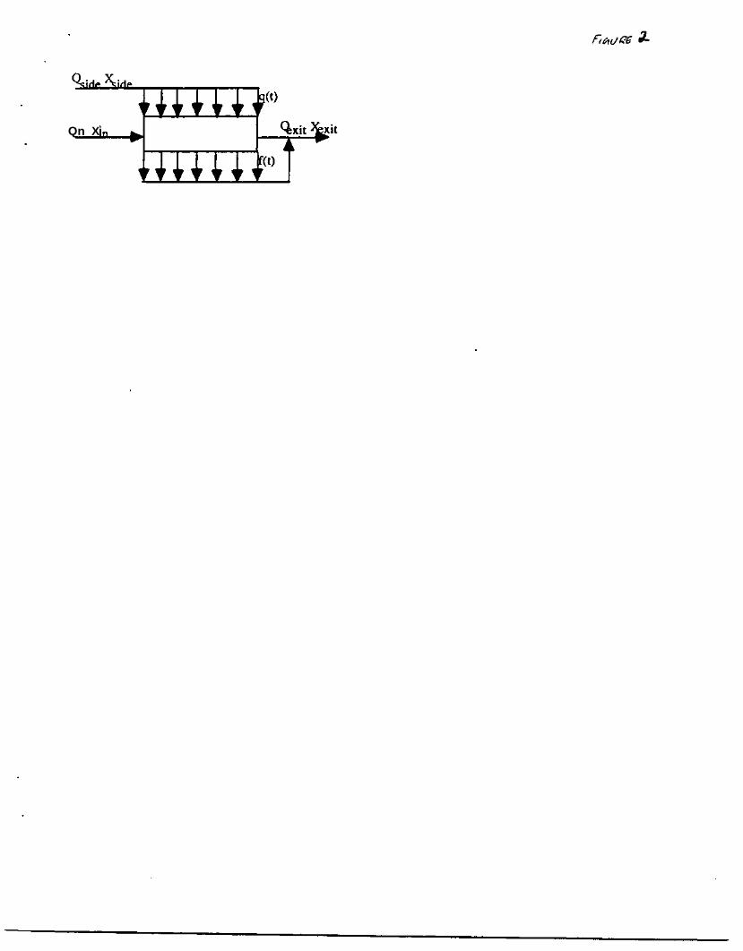
A Differential Sidestream Reactor is a PFR with sidestream addition along the length of

the reactor, as illustrated in Figure 2. Here, Qside. Qin* Qexit and Xside> Xin, Xexit are

the sidestream, feed and exit flowrates and concentrations, respectively. In this model we

assume that the sidestream composition remains constant along the length of the reactor and

instantaneous mixing between the sidestream and the reactor stream occurs. Let a

represent distance along the length of the reactor and consider a segment 5a, f(a)5a is the

fraction of Qexit (i-c. Qside + Qin) which leaves the reactor between a and a+Sa. Here,

let q(a) 5a be the fraction of Qside entering the reactor between a and a + 5a and let

Q(a) be the total molar flow at a (for simplicity we consider constant density systems,

although variable density systems may be considered by a straightforward extension). A

differential mass balance on 5a yields equation (2.1) and the NLP model may be

formulated as in P2.1.

Max J(XDSR exit, t)(P2.1)

q, f,T

dX/da = R(X(a), T(a)) + (q(a) Qside / Q(a)) ( Xside - X(a)) (2.1)

X(0) = Xfeed + q(0) Xside (2.2)

XDSR exit = or f(a) X(a) da (2.3)

1 = oJ °° f«x) da (2.4)

1 = ol °° q(a) da (2.5)

x = oJ °° J a (q(a') Qside / Qexit - f(af)) <*<*' da (2.6)

TDSR exit = J °° f(a) T(a) da (2.7)

where R(T(a), X(a)) is the temperature dependent rate of reaction, and X(a) and T(a) are

the mass concentrations and temperature at a, respectively. Here, XQSRexit and TDSRexit

are the mass concentration and temperature at the exit of the DSR and x is the mean

residence time in the DSR. Equations (2.1) and (2.2) are the differential equation and

initial conditions to the DSR. Equation (2.3) is the mean outlet concentration from the

DSR, equations (2.4) and (2.5) are the normalization equations for f and q. The last two

equations (2.6) and (2.7) give the mean residence time distribution and exit temperature for

the DSR:

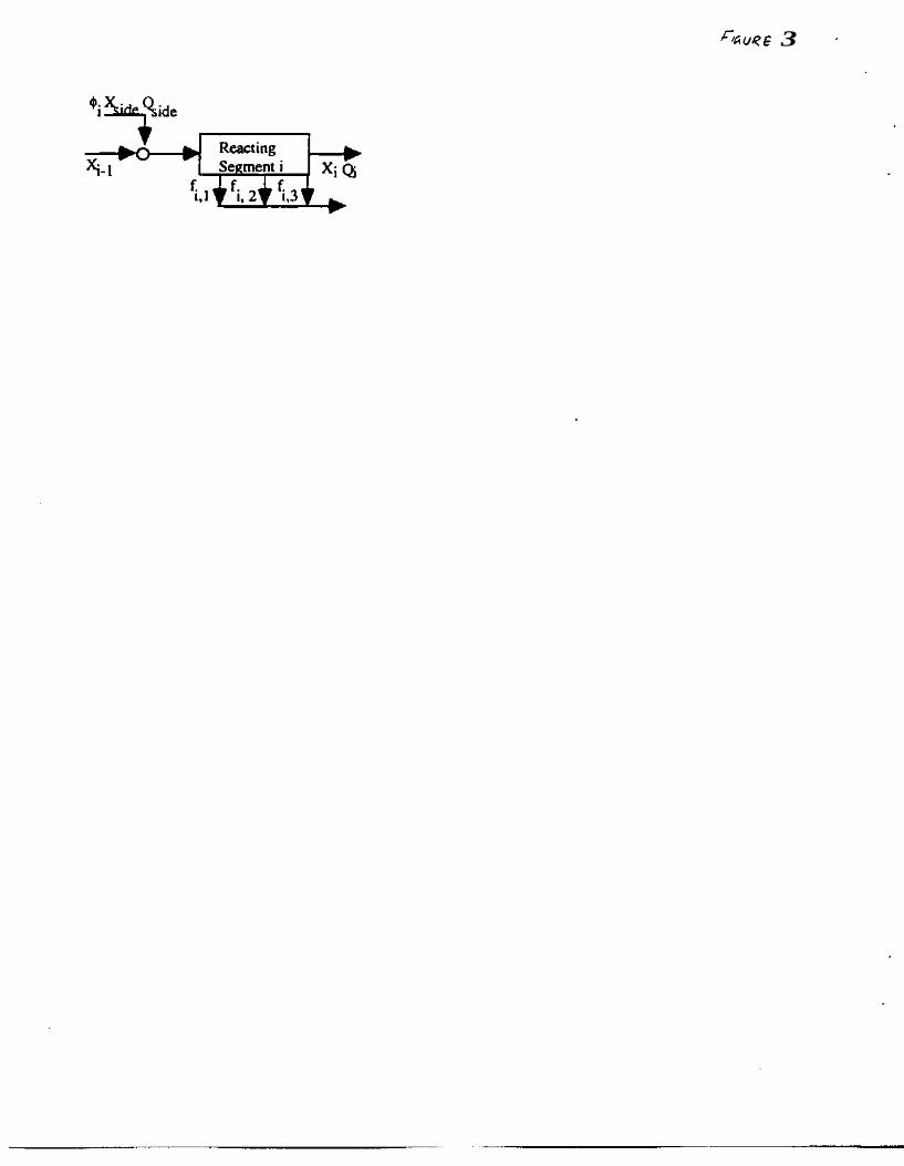
This is an optimal control problc;:: where the control profiles are q, i" und T. The

problem is simplified by discretizing the reactor into elements with finite mixing points in

between as shown in Figure 3. This approximates the DSR by the set of differential

equations for the i* reacting segment:

dXj/da = R(Xi(a), Tj(a)) over a j < a < a i + i , with Xj(ai) = Xi-i + <t>iQside Xside

Here (f>j is the fraction of the flow added at the i**1 reacting element inlet and <J>i Qside is a

discrete approximation to q(a)Qside/Q(o0 in (2.1). This DSR representation simplifies to

the cold shot cooling reactor or cross flow reactor, proposed by Balakrishna and Biegler

(1992b). when the sidestrcam conditions are identical to those of the feed stream.

We next discretize the differential equations in each reacting segment by using

orthogonal collocation, with NE reacting segments or elements and K collocation points in

each element. Figure 3 shows the discretized model, where the subscript m denotes the i1*1

reacting element and j denotes the j1*1 collocation point. Over each finite element, the

concentration, X(a), and the other profiles, are approximated by a piecewise polynomial

represented by Lagrange basis functions (Lk(a)) and defined as:

X(a) = Y Xik Lk(a) for a i o < a < aj+ ] o. and. Lk(a) = n [5LL^ iL]i=O;k

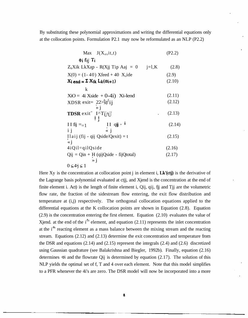
By substituting these polynomial approximations and writing the differential equations only

at the collocation points. Formulation P2.1 may now be reformulated as an NLP (P2.2)

Max J(Xexit,t) (P2.2)

XiO =

XDSR

TDSR

I I fij =

k4i Xside +exit= 22>

» jexit= I^T

i i1 J

= 1

0-4i)MJ

fij

UfU

I I qij

Xi-lend

= i

ZkXik LkXap - R(Xjj Tip Aaj = 0 j=l,K (2.8)

X(0) = (1- 40) Xfeed + 40 Xside (2.9)(2.10)

(2.11)(2.12)

. (2.13)

j (2.14)i j « jI l a i j (fij - qij Qside/Qexit) = t (2.15)« j4iQil=qi lQside (2.16)Qij = Qin + H (qijQside - fijQtotal) (2.17)

» j0 < 4>j < 1

Here Xy is the concentration at collocation point j in element i, Lk'(ctj) is the derivative of

the Lagrange basis polynomial evaluated at ctjj, and Xjend is the concentration at the end of

finite element i. Act) is the length of finite element i, Qij, qij, fjj and Tjj are the volumetric

flow rate, the fraction of the sidestream flow entering, the exit flow distribution and

temperature at (i,j) respectively. The orthogonal collocation equations applied to the

differential equations at the K collocation points are shown in Equation (2.8). Equation

(2.9) is the concentration entering the first element. Equation (2.10) evaluates the value of

Xjend. at the end of the i tn element, and equation (2.11) represents the inlet concentration

at the i t n reacting element as a mass balance between the mixing stream and the reacting

stream. Equations (2.12) and (2.13) determine the exit concentration and temperature from

the DSR and equations (2.14) and (2.15) represent the integrals (2.4) and (2.6) discretized

using Gaussian quadrature (see Balakrishna and Biegler, 1992b). Finally, equation (2.16)

determines <t>i and the flowrate Qij is determined by equation (2.17). The solution of this

NLP yields the optimal set of f, T and 4 over each element. Note that this model simplifies

to a PFR whenever the 4i's are zero. The DSR model will now be incorporated into a more

general reactor module that will be used make up the MINLP formulation for reactor

network synthesis.

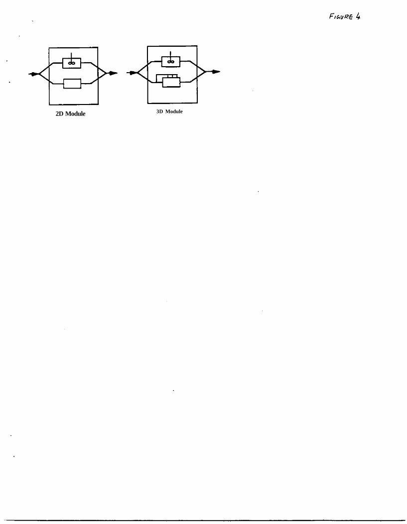
2.3 The Reactor Module

The attainable region properties described in section 2.1 are used to postulate a reactor

module, which can be linked with a forward connectivity to other modules. These

properties suggest that the boundary of the attainable region is formed by PFR segments

and straight lines. The reactor structures which need to be considered are PFR's and

CSTR's when there are only two independent problem dimensions and PFR's, CSTR's

and DSR's for higher dimensions. Recycle systems (both individual recycle reactors and

global recycles around a network of reactors) need not be considered, and this reduces the

complexity of the module. Hence a two dimensional reactor iriodule consists of a PFR and

a CSTR, and for higher dimensional problems it is made up of a DSR and a CSTR (A

separate PFR model need not be considered in higher dimensional problems since the DSR

without the sidestream is a PFR). A typical reactor module is shown in Figure 4, and a

binary variable is associated with each reactor path in a module. For instance, if the DSR is

chosen in the ith reactor module, Yjd, the binary variable associated with it, is set equal to

one. These reactor modules form the key part of the reactor network synthesis algorithm.

2.4 Reactor network synthesis algorithm

The problem is formulated as an MINLP (P2.3) below. Here we link the reactor

modules shown in Figure 4 with a forward connectivity. These links lead to networks that

have bypasses, serial structures and parallel structures embedded within them as shown in

Figures 5 and 6. Note that this formulation does not contain recycle reactors or interunit

recycles as these cannot form the boundary of the attainable region. Within the i* module

we have the equations that describe both CSTRs and DSRs (or PFRs in the two

dimensional case). The feeds to module i are made up of upstream reactions and bypasses,

from modules k. The outlet streams of these modules are then passed downstream until the

exit concentration, Xexit> is determined. The resulting optimization problem is given by:

Max J(Xcxit,T)(P2.3)

q.f.T

XcSTR(i) = R(XcSTR(i) TcSTR(i)) tC(i) + Xo i (2.18)

dXDSR(i)/da=R(X«x)(XDSRO(i) = Xo(i)XDSRexit(i)= ol tmax

1 = 0Jtmax f(ot(i)) da(i)1 = oltmax q(ot(i)) da(i)x = 0 I t m a x o J 0 ^(2.24)TDSRexit(i) = J t m a x

i)) Qside(i)/Qa(i))( Xside(i) -

)) dct(i)

Qside(i) / Qexit(i) -

)) dot(i)

(2.19)(2.20)(2.21)(2.22)(2.23)da ( j )

(2.25)

Fif = 2 FRi-lk=0

(2.26)

FjfXif = I Fid-iXk

k=0(2.27)

Xif = Xjc in = Xid inFif = F ic + FidFjfXi= FjcXi

N

(2.28)(2.29)(2.30)

(2.31)

(2.32)

0<Fic<U*Yic 0<Fid<U*Yid Y i ce{O,l} Yid e {0,1}

Here Fjf is the flowrate at the inlet of the itn reactor module; Fki-1 * Xki-1 are the flowrateand concentration from the exit of the kth stage, which is an inlet stream to the ith stage(k=0, i-1). Xif is the concentration at the inlet to the itn reactor module; Fjc, Fjd are theflowrates of the stream passing through the CSTR and DSR in the itn reactor module; Xjcin, Xjc, Xjd in. and Xjd are the concentration at the inlet and exit of the CSTR and DSRrespectively in the itn reactor module. Finally, Xj is the concentration at the exit of the itn

reactor module and Yjc and Yjd are the binary variables associated with the CSTR and DSRin the itn reactor module. Equations (2.18)-(2.25) constitute the reactor module at stage imade up of a CSTR (2.18) and a DSR (2.19)-(2.25). The inlet conditions to the module

10

and the individual reactors are given by (2.26)-(2.29). Equation (2.30) represents the exit

from the i t h module and equation (2.31) ensures that only one among the two reactors is

chosen in the i th module. The exit from the ith reactor module forms the inlet to any one or

a combination of modules i+1 to N as shown in equation (2.32).

From Figures 5 and 6, serial structures may be easily visualized since the algorithm is a

stepwise constructive technique. In Figure 5 the feed conditions (Fjf, Xjf) to i^1 module

may be the exit conditions of any one or a combination of the previous i-1 modules.

Equations (2.26) and (2.27) illustrate this fact. Hence when the i t h reactor module

extension is considered, bypasses from the exits of the previous i-2 modules and the feed

are automatically considered. Similarly, parallel reactor structures up to the i-lth module

are also accounted for. This structure keeps the constructive MINLP algorithm as compact

as possible. In the i* reactor module either the CSTR or the DSR may be chosen and the

exit conditions from the i**1 reactor module (Xj) are determined appropriately. This is

represented by equations (2.28), (2.29) (2.30) and (2.31). The exit stream from the i th

reactor module forms the inlet stream to any one or a combination of reactor modules i+1 to

N (2.32). Figure 6 depicts the parallel structure; here the feed stream to the ith and i+1^

modules are identical and the exits of these modules combine to form the inlet to the 1+2*

module. Similarly, up to N parallel structures may be realized where N is the number of

reactor modules in the optimization.

The MINLP formulation can be solved directly using standard algorithms such as Outer

Approximation or Generalized Benders Decomposition. Both approaches require alternate

solutions of MILP and NLP subproblems. However, because (P2.3) is a nonconvex

optimization problem, there is a possibility of finding snbopfimal solution when local NLP

methods are applied. Avoiding this difficulty requires the application of global optimization

methods (see, e.g., Floudas and Grossmann, 1995, for a review) and encouraging

approaches for reactor networks are being developed (Pantelides and Smith, 1995). These

methods, however, can still be very expensive for the large problems considered in this

study. Instead, to ensure good solutions we solve an improving sequence of MINLP

problems according to the following steps.

1) Solve a segregated flow model to obtain a lower bound on the solution. This

formulation is usually a linear program with a guaranteed global solution

(Balakrishna and Biegler, 1992a).

11

2) Initialize the first reactor module with the solution obtained from step J and

optimize it with respect to a specific objective. The inlet conditions to the reactor

module are the feed conditions. This yields an initial target to the attainable region.

In addition, it does not eliminate the 'CSTR1 path, but only makes it inactive with a

zero binary variable.

3) Extend the first module with an additional reactor module. The feed to the

second module is the exit from the first or a combination of the fresh feed and the

exit of the first module. If this extension improves the objective then further

extensions need to be considered else the optimal network is assumed to have been

found.

4) Ensure that the feed to the i*h reactor module extension may be the exit of any

one or a combination of the exits of the previous i-1 modules or the initial feed.

5) Account for bypass streams by ensuring that the exit from the ith reactor module

plus the bypasses from the exits of any one or a combination of the previous i-1

modules form the inlet to the i + 1 * reactor module.

An additional disadvantage is that equations (2.27) and (2.30) are bilinear and it is

possible that for some initializations of the binary variables, the MDLP master problem may

eliminate feasible regions and therefore not consider favorable options in the superstructure

(Kocis, 1988). This can be remedied by reformulating the bilinear equations using the

modeling/decomposition strategy with appropriate under-approximators. However these

underestimators may not be easy to generate. Also, initialization of the continuous

variables plays a significant role because of the extreme nonlinearity of the models. In the

examples presented in the next section, a lower bound to the objective was determined by

solving a PFR model, the DSR's in the reactor modules were initialized as PFR's and the

binary variables associated with them were initialized to one. This initialization procedure

was observed to be effective in avoiding these difficulties.

The resulting compact MINLP structure is a constructive technique; alternative reactor

paths are considered by the use of reactor modules. The optimal reactor structure is

determined at each stage but other paths are not eliminated. For instance, parallel reactor

structures or bypass structures up to the i - 1 * module will be realized while considering the

i*h reactor module extension, if they exist at the optimum. The exit streams of the upstream

reactor modules in parallel or bypass mix to form the inlet stream for the next reactor

module. The advantages of this approach are:

12

1) The MINLP combines attainable region properties and superstructure techniques

2) The network is sufficiently rich to yield the optimum network

3) The approach overcomes the need for monotonic objective improvement as in the

B&B approach.

4) The MINLP realizes parallel structures and bypasses automatically if they exist

at the optimum

5) Higher dimensional problems are addressed directly through the MINLP

formulation.

In addition, the algorithm allows for complete forward connectivity in the reactor

network. Hence, reactor structures which are not considered directly in the algorithm can

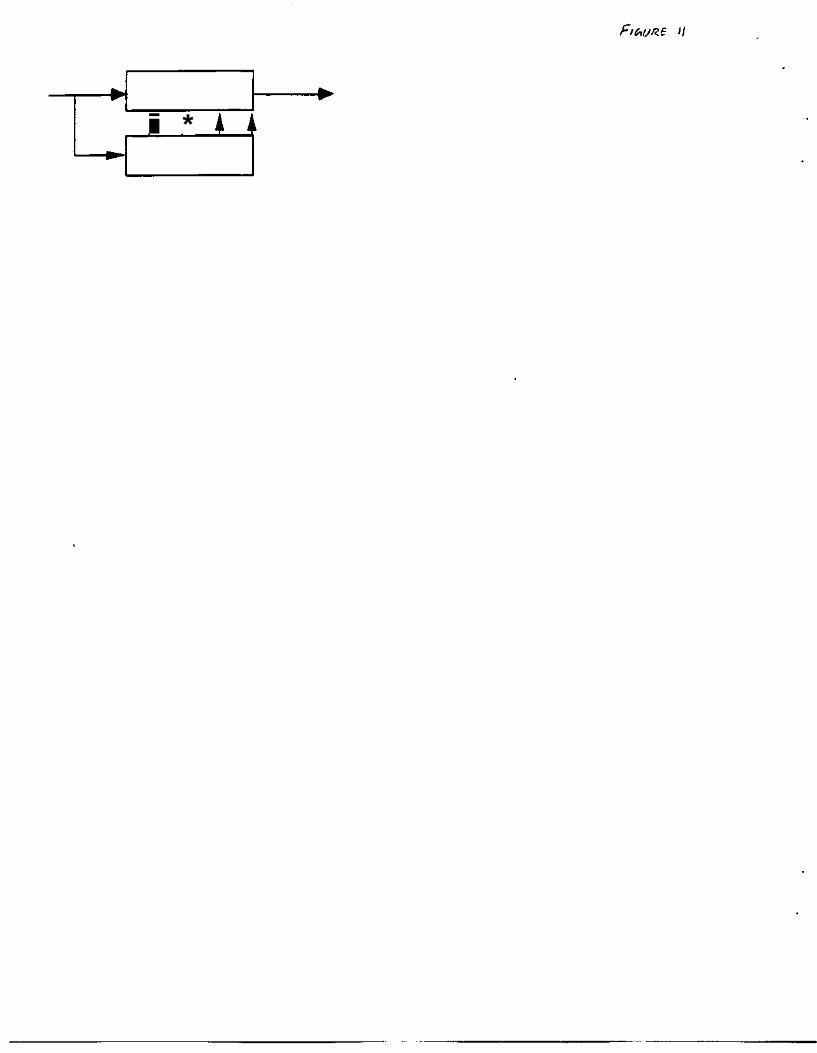
still be realized. An interesting example is a DSR with a variable composition sidestream

feed taken from side exits of a PFR, as shown in Figure 11. Hopley (1995) recently

derived such a network with attainable region constructions and in Appendix B, we show

that such a structure is also allowed by our MINLP formulation. In the next section we

illustrate this MENLP approach on a variety of reactor network synthesis problems.

3. Reactor network examples

In order to demonstrate the performance of the algorithm, five examples from B&B

(1992a) were solved using the new technique. The kinetic models and reaction conditions

are given in Appendix C. The results of the optimization are:

Examplenetwork

sec)

1. a Pinene

2. Trambouze

3. Denbigh I

4. Denbigh II

5. Van do Vusse I

XB

xcxc

XB

XB

Objective

Max

/ ( 1 - X A )

/XD

Optimal Value

(Solution time, sec)

B&B

1.480(0.13)

0.500(0.10)

3.540 (0.22)

1.322(0.07)

0.736 (0.05)

MINLP

1.480(0.16)

0.500(0.11)

3.540 (0.60)

1.322(0.10)

0.736 (0.07)

Reactor

(Residence time,

PFR (60)

CSTR (7.5)

PFR (0.766) +

CSTR (3505)

PFR (0.209)

PFR (0.262)

13

All the MINLP models were solved using DICOPT++ (Viswanathan and Grossmann,

1990), which is interfaced to the GAMS (Brooke et al, 1988) modeling system, on a HP

9000-720 workstation. The MENLP algorithm yields identical solutions as compared to the

earlier algorithm. All of these solutions have been shov\n to be globally optimal

(BalakrishnaandBiegler, 1992a, Hildebrandt et al, 1990). The solution times are slightly

higher than those observed using the B&B algorithm. However the new algorithm allows

the designer to find solutions which involve complex reactor networks and finds the best

solution even if the objective improvement is nonmonotonic as seen in the examples which

follow.

Example 6 (Isothermal Reactor Network Synthesis). The isothermal Van de Vusse

reaction involves four species for which the objective is the maximization of the yield of the

intermediate species B, starting with a feed of pure A. The reaction kinetics is given by

D

R(X) = [ - X A - 20 XA2 , X A - 2 XB, 2 XB, 20 X A

2

The B&B algorithm yields a sub-optimal network of a recycle reactor (recycle ratio =

0.772, T = 0.1005 sec) in series with a PFR (x = 0.09 sec) with a yield of 0.069 and a

computational time of 0.038 sec on a HP-UX 9000-720 workstation.

The constructive MINLP approach was applied to this 2D problem ( X A and XB are the

two independent dimensions). Each reactor module consists of a CSTR and a PFR. The

optimal network was found to be a CSTR (0.302 sec, X = 0.059) followed by a PFR

(0.161 sec, X = 0.0703) with an optimal yield of 0.0703. This solution is confirmed by

the geometrical attainable region technique of Hildebrandt and Glasser (1990). The

computational time on a HP-UX 9000-720 workstation is 0.041 sec, which is almost the

same as that taken by the B&B approach. Attainable region properties 1) and 3) from

section 2.1 were used to make the MINLP as compact as possible.

Note that the B&B algorithm could not identify this network solution because the yield

obtained from the recycle reactor at the end of the first stage (X=0.063) is higher than that

obtained by the CSTR (X=0.059). Hence, the B&B algorithm picked the recycle reactor

and considered extensions from it. However, a PFR extension from this CSTR, which is

14

suboptimal in the first stage, improves the objective more than any extension from the

recycle reactor. The constructive MINLP technique achieves the optimum by not

eliminating suboptimal solutions until the final stage has been reached. Thus, the problem

of nonmonotonic objective improvement is overcome.

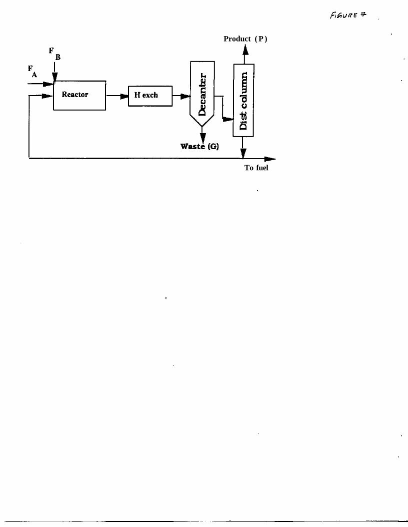
Example 7 (Reactor flowsheet integration). The reactor network synthesis procedure is

coupled with the simultaneous solution strategy for reactor flowsheet integration. The

Williams-Otto flowsheet, a typical flowsheet optimization problem (Ray and Szekely,

1973), is considered in this optimization. The schematic diagram of the flowsheet is

shown in Figure 7. The raw materials A and B are fed to the reactor, where they react to

form an intermediate C, desired product P, byproduct E and waste product G. The rate

vector for the components A, B, C, P, E and G respectively is given by

R(x) = [ -ki X A X B ; - ( ki X A + k 2 X c ) X B ; 2 ki X A X R - 2 k2 X B X(>

k3 Xp Xc; k2 X B X C - k3 Xp Xc; 2 kc X B X C ; 1.5 k3 Xp X c ]

where k i = 110.695 wt frac h'l< ko = 561.088 wt frac h"1, k3 = 1248.748 wt frac h"1

and the X's denote the weight fractions of the components. The reaction scheme is given

by

A + B — V CC + B — ^ P + E

P + C —^ G

The effluent from the reactor is cooled in a heat exchanger, followed by a decanter where

the waste product G is separated from the other components. The waste G is then treated

in a waste treatment plant while the remaining components are fed to a distillation column

which separates the desired product P. Some of the bottoms product from the distillation

column is recycled to the reactor inlet and the rest is used as fuel.

The objective function considered in the optimization is an annualized net profit which

includes sales, cost of raw materials, sales and research expenditure, utility cost,

depreciation costs and the last term annualizes the capital cost.

J = (8400 * ( 0.3 Fp + 0.0068 FD - 0.02 FA - 0.03 Ffi ) - 0.124 *

( 8400 ) * ( 0.3 Fp + 0.0068 FD ) - 2.22 FR - 0.1 * ( 6 FR * t ) -

0.33 * ( 6 F R * t )

!5

where FA, FB and Fp are the flow rates of A, B and pure P. Fp is fixed at the desired

level. FD is the purge flow rate and FR is the total flow of components within the reactor.

The variable t denotes the residence time in the complete reactor network. The reactor cost

is a function of residence time and is irrespective of the reactor type. This assumption is

reasonable since the capital cost of the reactor is usually much smaller than the operating

costs.

The reactor in the flowsheet is replaced by a 3D reactor module consisting of a DSR

and a CSTR. The constructive MINLP algorithm for optimal reactor synthesis is combined

with the constraints imposed by the process flowsheet. The production rate of waste G is

assumed to be constrained by an environmental regulation to be a maximum of 11.5 lb/hr.

The optimal reactor network was found to be a PFR (DSR without sidestream addition) and

the maximum annualized profit was found to be $135.21 * 1000 $/yr for a production rate

of 2720 lb/hr of desired product P. The residence time in the PFR was found to be 0.1 hr.

If the residence time is restricted to a maximum of 0.02 hr, the profit was found to be

$133.21 * 1000 $/yr in a plug flow reactor as in Lakshmanan and Biegler, 1995. Reactor

module extensions did not improve the objective. The computational time taken on HP-UX

9000-720 workstation was 2.09 CPU seconds. Note that the space of initial conditions of

the streams entering the reactor network is not fixed, but is bounded by flowsheet

constraints.

Example 8 (Nonisothermal Reactor Network Synthesis). The sulfur dioxide oxidation

reaction considered in this example is exothermic and reversible. The reaction follows

complex kinetics and it is assumed that the reaction occurs at constant pressure. The extent

of reaction, g is defined as the number of moles of sulfur trioxide formed per unit mass of

mixture.SO2 + 1/2 02 » SO3

R(g,t) = 3.6*103[exp(12.07-50/(l+0.311t)) ((2.5-g)0-5(3.46.0.5g)/(32.01-0.5g)1-5)

- exp(22.75-86.45/( 1+0.31 It)) g(3.46-0.5g)°-5/((32.01-0.5g)(2.5-g)0-5)]

kg mole SO3/hr/kg catalyst

where t= (T-To)/J T is the temperature of the mixture in °C

J is assumed to have an average value of 96.5 K Kg/mol

The specific heat of the mixture is assumed to be constant, so the energy balance is

represented by T-To = J(g-go) where To is the temperature of the mixture at extent go.

The feed has a composition of 7.8 mol % SO2, 10.8 mol % O2 and 81.4 mol % N2 at a

temperature of 37°C, a pressure of 1 atm, and a flowrate of 7731 kg/hr. The feed may be

16

preheated. The objective is to maximize the extent of the reaction. Two cases are

considered, the nonadiabatic and the adiabatic case.

Case a) Nonadiabatic nonisothermal reactor network synthesis

The nonadiabatic case was solved by Balakrishna and Biegler (1992b). They found the

optimal reactor network to be a PFR with a falling temperature profile. The maximum

extent of reaction was a function of the residence time (x) with g=2.42 at x=0.25 sec,

g=2.48 at x=2.5 sec and g reaches 2.5 asymptotically at large residence times. The rate of

the reaction is high at high initial temperatures. Hence, an arbitrarily high preheat

temperature of 600°C was used.

Case b) Adiabatic nonisothermal reactor network synthesis '

Intuitive reasoning suggests that a falling temperature profile would optimize the extent

of reaction since the reaction is exothermic. However, adiabatic restrictions make it

difficult to maintain a falling temperature profile, unless a cold shot cooling reactor or a

DSR with side stream colder than the reactor temperature, were used. Many researchers

have worked on this problem, Lee and Aris (1963) suggested a preheater followed by a 3

stage cold shot cooling reactor. Melange and Villermaux (1967), Helinckx and Van

Rompay (1968) and Melange and Vincent (1972) suggested a preheater followed by a cold

shot cooling reactor with 3 or more stages. Glasser et al (1992) suggested a serial

combination of a preheater followed by a CSTR, PFR, DSR and PFR to be the optimal

reactor network for this reaction.

The constructive MINLP approach was applied to this 3D problem (preheating of the

feed introduces a third dimension T, in addition to g and t ) . The allowable preheat

temperature range was chosen to be 520 °C - 615 °C. Here, the reactor module consists of

a CSTR and a DSR. This problem required four stages of the algorithm. The optimal

preheat temperature was found to be 538.5 °C with an optimal network of a serial

arrangement of a CSTR (X=0.232, T=560.9 °C) followed by a PFR (X=0.283, T=564.3

°C), a DSR (X=2.426, T=398.9 °C) and finally a PFR giving an optimal extent of reaction

of g=2.48 with T=403.9°C. The optimal network is shown in Figure 8. The

computational time taken on a HP-UX 9000-720 workstation was 3.69 CPU sec. The

results of our approach match the results of the graphical technique of Glasser et al (1992).

17

3. Conclusions

A compact MINLP approach to reactor network synthesis which synergistically

combines superstructure and previous targeting techniques has been proposed. This

constructive algorithm targets the attainable region by making use of reactor modules.

Various attainable region and superstructure properties derived from geometric targeting

techniques were used to simplify the reactor module and to ensure that the superstructure is

sufficiently rich to yield optimal reactor networks. Some other features of the algorithm are

that parallel reactor structures and bypasses are identified automatically, if they exist for the

optimal network, and the new algorithm overcomes the need for monotonic improvement

of the objective at each iteration. The constructive MINLP algorithm attempts to find the

best solution with available optimization techniques. It first specifies a lower bound on the

objective by optimizing a segregated flow target from the feed and then uses this solution to

initialize the next module. This procedure ensures that the stagewise solutions steadily

improve without discarding inactive parts of the candidate network. Also, higher

dimensional problems may be solved by using this algorithm. For this purpose complex

reactor structures which appear in higher dimensional problems have been incorporated in

the reactor module.

The nonconvexity of the reactor models and the rate equations require that the algorithm

be made as simple as possible. The constructive nature of the algorithm ensures that only

the simplest model which needs to be considered at each stage is solved. Also, the absence

of recycles reduces the nonlinearity of the model. However, the resulting approach is an

MINLP technique and may be computationally expensive. The feasibility and versatility of

this algorithm is demonstrated by solving a set of examples with varying complexity. Five

small examples were solved initially in order to show the feasibility and dependability of

the algorithm. In addition, Example 6 demonstrates how the algorithm overcomes the need

for monotonic improvement in the objective, Example 7 integrates the synthesis of the

reactor network with the process flowsheet, which could be difficult and tedious using

geometric techniques, and the eighth example demonstrates how complex reactor networks

may be realized by using this constructive technique.

Hence, the MINLP algorithm is quite comprehensive. It is a versatile algorithm which

allows the designer to incorporate additional attainable region properties when necessary.

In addition, reactor structures which are more complex than those considered in the

modules may be realized as shown in Appendix B.

18

AcknowledgmentThis research was partially supported by the Engineering Design Research Center, an NSF

sponsored engineering center at CMU, and the Department of Energy.

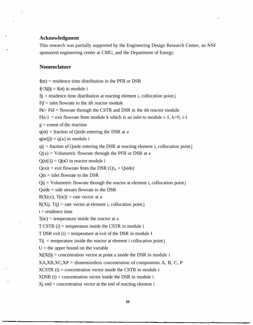
Nomenclature

f(oc) = residence time distribution in the PFR or DSR

f(<X(i)) = f(ot) in module i

fij = residence time distribution at reacting element i, collocation point j

Fjf = inlet flowrate to the ith reactor module

Fic> Fid = flowrate through the CSTR and DSR in the ith reactor module

Fki-1 = exit flowrate from module k which is an inlet to module i-1, k=0, i-1

g = extent of the reaction

q(ot) = fraction of Qside entering the DSR at a

q(oc(j)) = q(a) in module i

qij = fraction of Qside entering the DSR at reacting element i, collocation point j

Q(a) = Volumetric flowrate through the PFR or DSR at a

Q(tt(i)) = Q(oO in reactor module i

Qexit = exit flowrate from the DSR (Qin + Qside)

Qin = inlet flowrate to the DSR

Qij = Volumetric flowrate through the reactor at element i, collocation point j

Qside = side stream flowrate to the DSR

R(X(cc), T(oc)) = rate vector at a

R(Xij. Tij) = rate vector at element i, collocation point j

t = residence time

T(oc) = temperature inside the reactor at a

T CSTR (i) = temperature inside the CSTR in module i

T DSR exit (i) = temperature at exit of the DSR in module I

Tij = temperature inside the reactor at element i collocation point j

U = the upper bound on the variable

X((X(i)) = concentration vector at point a inside the DSR in module i

XA,XB,XC,XP = dimensionless concentration of components A, B, C, P

XCSTR (i) = concentration vector inside the CSTR in module i

XDSR (i) = concentration vector inside the DSR in module i

Xj end = concentration vector at the end of reacting element i

19

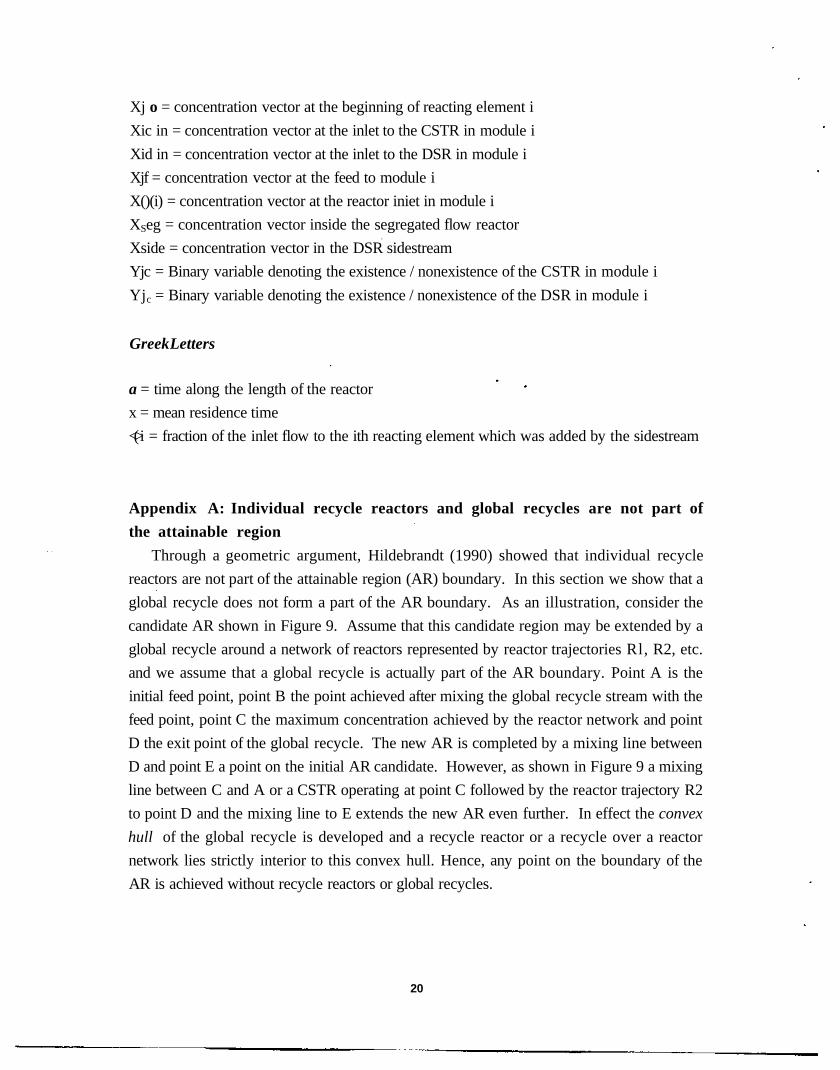
Xj o = concentration vector at the beginning of reacting element i

Xic in = concentration vector at the inlet to the CSTR in module i

Xid in = concentration vector at the inlet to the DSR in module i

Xjf = concentration vector at the feed to module i

X()(i) = concentration vector at the reactor iniet in module i

XSeg = concentration vector inside the segregated flow reactor

Xside = concentration vector in the DSR sidestream

Yjc = Binary variable denoting the existence / nonexistence of the CSTR in module i

Yjc = Binary variable denoting the existence / nonexistence of the DSR in module i

Greek Letters

a = time along the length of the reactor

x = mean residence time

<(>i = fraction of the inlet flow to the ith reacting element which was added by the sidestream

Appendix A: Individual recycle reactors and global recycles are not part of

the attainable region

Through a geometric argument, Hildebrandt (1990) showed that individual recycle

reactors are not part of the attainable region (AR) boundary. In this section we show that a

global recycle does not form a part of the AR boundary. As an illustration, consider the

candidate AR shown in Figure 9. Assume that this candidate region may be extended by a

global recycle around a network of reactors represented by reactor trajectories Rl, R2, etc.

and we assume that a global recycle is actually part of the AR boundary. Point A is the

initial feed point, point B the point achieved after mixing the global recycle stream with the

feed point, point C the maximum concentration achieved by the reactor network and point

D the exit point of the global recycle. The new AR is completed by a mixing line between

D and point E a point on the initial AR candidate. However, as shown in Figure 9 a mixing

line between C and A or a CSTR operating at point C followed by the reactor trajectory R2

to point D and the mixing line to E extends the new AR even further. In effect the convex

hull of the global recycle is developed and a recycle reactor or a recycle over a reactor

network lies strictly interior to this convex hull. Hence, any point on the boundary of the

AR is achieved without recycle reactors or global recycles.

20

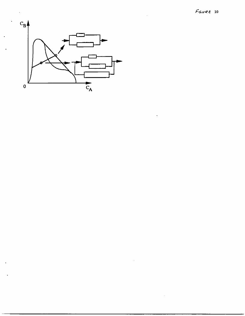
Any point on the boundary of an N dimensional attainable region may

be achieved by N parallel structures: This property was shown by Feinberg and

Hildebrandt (1992) and is illustrated for the two dimensional attainable region formed by a

PFR trajectory with the concavity in the trajectory filled by a mixing line. From Figure 10

we see that any point on the boundary of the attainable region may be achieved by 2 parallel

reactor structures and any point on the interior may be represented by 3 parallel structures.

Appendix B: DSR with the sidestream composition varying along thelength of the reactor.Hopley (1995) suggested that in complicated adiabatic exothermic reversible reactions, a

DSR with the sidestream originating from a PFR may exist (Figure 11). Although such a

DSR is not considered in the reactor module, the fact that the algorithm allows for complete

forward connectivity enables us to approach such a reactor structure in the limit, as shown

in Figure 12a and 12b. Figure 12a shows the structure of the reactor modules which will

be chosen at the optimum, if a DSR like that shown in Figure 11 exists at the optimum.

The PFR (DSR without the sidestream) may be picked in each of the modules resulting in

the structure shown in Figure 12b. This structure is an approximation to the DSR in Figure

11.

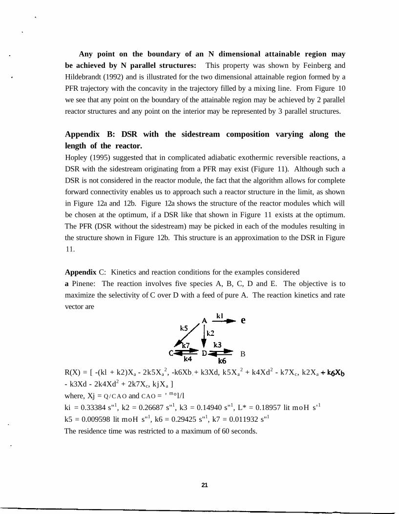
Appendix C: Kinetics and reaction conditions for the examples considered

a Pinene: The reaction involves five species A, B, C, D and E. The objective is to

maximize the selectivity of C over D with a feed of pure A. The reaction kinetics and rate

vector arekl- e

B

R(X) = [ -(kl + k2)Xa - 2k5Xa2, -k6Xb + k3Xd, k5Xa

2 + k4Xd2 - k7Xc, k2Xa

- k3Xd - 2k4Xd2 + 2k7Xc, kjXa ]

where, Xj = Q / C A O and CAO = ' m°l/l

ki = 0.33384 s"1, k2 = 0.26687 s"1, k3 = 0.14940 s"1, L* = 0.18957 lit moH s'1

k5 = 0.009598 lit moH s"1, k6 = 0.29425 s"1, k7 = 0.011932 s"1

The residence time was restricted to a maximum of 60 seconds.

21

Trambouze: The Trambouze reaction involves four components and has the following

reaction schemekl k2 k3

where, kl = 0.025 lit mol"1 min"1, k2 = 0.2 min"1 and k3 = 0.4 lit mol"1 min"1

Denbigh I: The isothermal Denbigh involves five species. The objective is to maximize the

production of C subject to 95% conversion of A. The reaction scheme and rate vector are

A k 1 ^ k2

k3 iD E

R(X) = [ -Xa(k3 + kiXa), k]Xa2 - Xb(k4Xb + k2), k2Xb,

where ki = 6 lit mol'1 s"1, k2 = k3 = 0.6 s"1, k4 = 0.6 lit mol'1 s"1, CAO = 6 mol/1

Denbigh II: The objective function considered is maximize Xb/Xd and the rate vector is

R(X) = [ -Xa(k3 + kiXa), 0.5kiXa2 - Xb(k4Xb + k2), k2Xb, k3Xa,

where k] = 6 lit mol"1 s"1, k2 = k3 = 0.6 s"1, k4 = 0.6 lit mol"1 s"1, Cao = 6 mol/1

and CdO = 0.6 mol/1

Van de Vusse I: The objective is the maximization of the yield of intermediate species B,

given a feed of pure A. The reaction scheme is shown in Example 6) and the rate vector

considered here is

R(X) = [ -10 XA - 0.29 X A2 , 10 XA - XB , XB, 0.29XA

2 ]

References

Achenie, L.E.K.; Biegler, L.T. Algorithmic Synthesis of Chemical Reactor Networks

using Mathematical Programming. I&EC Fund. 1986, 25, 621.

Achenie, L.E.K.; Biegler, L.T. Developing Targets for the Performance Index of a

Chemical Reactor Network. I&EC Research. 1988, 27, 1811.

Balakrishna., S.; Biegler, L.T. A Constructive Targeting Approach for the Synthesis of

Isothermal Reactor Networks. / & EC Research. 1992a, 31(9), 300.

22

Balakrishna., S.; Biegler, L.T. Targeting Strategies for Synthesis and Energy Integration

of Nonisothermal Reactor Networks. / & EC Research. 1992b,31(9), 2152.

Balakrishna., S.; Biegler, L.T. A Unified Approach for the Simultaneous Synthesis of

Reaction, Energy, and Separation Systems. / & EC Research. 1993,32(7), 1372.

Brooke, A.; Kendrick, D.; Meeraus, A. GAMS: A User's Guide; Scientific Press;

Redwood City, CA, 1988.

Chitra, S.P.; Govind, R. Yield Optimization for Complex Reactor Systems. Chem. Eng.

Sci. 1981,36, 1219.

Chitra, S.P.; Govind, R. Synthesis of Optimal Reactor Structures for Homogenous

Reactions. AIChE J. 1985,31(2), 177..

Duran, M.A.; Grossmann, I.E. Simultaneous Optimization and Heat Integration of

Chemical Processes. AIChE J., 1986, 32,123.

Feinberg, M. and D. Hildebrandt, Optimal Reactor Design from a Geometric Viewpoint.

Paper 142c, AIChE Annual Meeting, Miami Beach, FL, 1992.

Floudas, C. and I. E. Grossmann, "Algorithmic Approaches to Process Synthesis: Logic

and Global Optimization," Foundations of Computer Aided Process Design '94, ATChE

Symposium Series, 91, L. T. Biegler and M. F. Doherty (eds.), p. 198 (1995)

Glasser, B.; Hildebrandt,D.; and Glasser,D. Optimal Mixing for Exothermic Reversible

Reactions. Ind. Eng. Chem. Res., 1992, 31(6), 1540.

Glasser, D.;. Crowe, C; Hildebrandt, D. A Geometric Approach to Steady Flow Reactors:

The Attainable Region and Optimization in Concentration Space. / & EC Research. 1987,

26(9), 1803.

Helinckx, L.G.; Van Rompay, P.V. Paper presented at the 97th event of the European

Federation of Chemical Eng., Florence, Italy; April 27-30, 1970.

Hildebrandt, D.; Glasser, D.: Crowe, C. The Geometry of the Attainable Region Generated

by Reaction and Mixing with and without Constraints. / & EC Research. 1990, 29(1), 49.

Hildebrandt, D. and L. T. Biegler, "Synthesis of Reactor Networks," Foundations of

Computer Aided Process Design '94, AIChE Symposium Series, 91, L. T. Biegler and M.

F. Doherty (eds.), p. 52 (1995)

Hopley, F.R. Optimal Reactor Structures: On Teaching and a Novel Optimal Substructure.

M.S. Thesis, University of Witwatersrand, Johannesburg, South Africa, 1995.

Horn, F. Attainable Regions in Chemical Reaction Technique. Presented at the Third

European Symposium on Chemical Reaction Eng., Pergamon, London, 1964.

Jackson, R. Optimization of Chemical Reactors with respect to Flow Configuration. J. opt.

Theory and applns. 1968, 2(4), 240.

23

Kocis, G. R. A Mixed-Integer Nonlinear Programming Approach to Structural Flowsheet

Optimization. Ph. D. thesis, Carnegie Mellon University, Pgh, PA, 1988.

Kokossis, A.C;. Floudas, C.A. Synthesis of Isothermal Reactor-Separator-Recycle

Systems. Presented at the Annual AIChE meeting, San Francisco, CA, 1989.

Kokossis, A.C; Floudas, C.A. Optimization of Complex Reactor Networks — I.

Isothermal Operation. Chem. Eng. ScL 1990, 45 (3), 595.

Kokossis, A.C, Floudas, C.A. Synthesis of Non-isothermal Reactor Networks. Presented

at the Annual AIChE meeting, San Francisco, CA, 1991

Lakshmanan, A. and L.T. Biegler, "Reactor Network Targeting for Waste Minimization,"

in Pollution Prevention via Process and Product Modifications, AIChE Symposium Series,

90, M. El-Halwagi and D. Petrides (eds.), p. 128 (1994)

Lee, K. Y.; Aris,R. Optimal Adiabatic Bed Reactors for Sulfur Dioxide with Cold Shot

Cooling. / & EC Proc. Des. & Dev., 1963, 2(4), 301.

Malenge, J.P.; Villermaux, J. Optimal Design of a Sequence of Adiabatic Reactors with

Cold Shot Cooling. I & EC Chem. Proc. Des. & Dev. 1967, 6, 535.

Malenge, J.P.; Vincent, L.M. Optimal Design of a Sequence of Adiabatic Reactors with

Cold Shot Cooling. I & EC Chem. Proc. Des. & Dev. 1967, 11(4),465.

Pantelides, C. and E. Smith, "A Software Tool for Structural and Parametric Design of

Continuous Processes," presented at Annual AIChE Meeting, Miami Beach (1995)

Viswanathan, J. V.; Grossmann, I.E. A combined penalty function and outer

approximation method for MINLP optimization. Comput. and Chem. Engg. 1990, 14,

769.

24

Table 1: Segregated flow reactor and continuous stirred tank reactor targeting

formulations for isothermal reactor network synthesis

PFR target CSTR target

Max J(Xexit) Max J(Xexit)

Xexit =ol tmaxf(0 Xseg(t)dt Xexit= Xo + R(X) xT = 0Jtmaxtf(t)dtJtmax f ( t ) dt _ i

dXseg/dt =

25

Figurel. An example of candidate attainable regions with nonmonotonic increase in the

objective.

Figure 2. Schematic of a Differential Sidestream Reactor.

Figure 3. Discretized element of a DSR for NLP formulation.

Figure 4. Reactor module for two and three dimensional problems.

Figure 5. Individual reactor module as a building block for the MINLP formulation.

Figure 6. An example of parallel structures from the MINLP formulation.

Figure 7. Williams Otto process flowsheet.

Figure 8. Optimal reactor network for the SO2 oxidation problem.

Figure 9. Illustration that global recycles are not part of the AR boundary.

Figure 10. Two dimension illustration of 2 reactors on the AR boundary and three within

the interior.

Figure 11. A DSR with the sidestream originating from a PFR.

Figure 12a. MINLP structure of the reactor modules at the approximate solution for

Figure 11.

Figure 12b. An approximation to the DSR in Figure 11.

26

0

AR optima

B&B optima

Qn Xj

3

2D Module 3D Module

5

Fki-lXki-l

Feed

Product ( P )

To fuel

4308.99 kg/hr

g=2.426T=398.9

g=2.48

7731 kg/hr

FlC* UJ?£

'BtD

Candidatettainable region

0

10

i *

~H>"\