SYNTHESIS OF MULTIPLE-PATTERN PLANAR ANTENNA ARRAYS WITH SINGLE

PREFIXED OR JOINTLY OPTIMIZED AMPLITUDE DISTRIBUTIONS

J. Brégains, A. Trastoy, F. Ares, E. Moreno

Grupo de Sistemas Radiantes, Departamento de Física Aplicada,

Facultad de Física, Universidad de Santiago de Compostela

15782 Santiago de Compostela, SPAIN

E-mail: faares@usc.es

Fax: +34 981547046

Key words: planar arrays, synthesis of multiple patterns with a common amplitude distribution

ABSTRACT: Previous work on the generation of multiple radiation patterns by a single linear

array antenna with an unchanging excitation amplitude distribution is generalized to planar

arrays. The amplitude distribution common to all the excitation distributions can be prefixed or

optimized jointly with the phase distributions.

1. INTRODUCTION

Since the size of antennas is fixed by physical considerations, the difficulty of accommodating

them on satellites and other facilities with multiple antenna-based functions grows with the

number of such functions if a separate antenna is used for each. In this context it is desirable for a

single antenna to be able to generate multiple radiation patterns, with the excitation

corresponding to each being selectable by suitable switching devices. However, it is also

desirable for the various excitation patterns delivered to a multiple-pattern array antenna to have

a common amplitude distribution, since implementation is technically more difficult for a

variable amplitude distribution than for a variable phase distribution.

Previous papers from our group have described the synthesis of linear multiple-pattern array

antennas in which the amplitude distribution common to all the excitations was prefixed so as to

ensure smoothness [1] or was optimized jointly with the various excitation phase distributions

[2]. In the latter case excitations were optimized directly, in the former a modified Woodward-

Lawson approach was used. The direct optimization method is here generalized, for both prefixed

and jointly optimized amplitudes, to planar array antennas, for which the joint optimization

problem has previously been approached by Bucci et al. [3] using projection operators in pattern

space.

2. DESCRIPTION OF THE METHOD

The array factor F(,) of an NM rectangular array of radiating elements laid out in the (x,y)

plane with its centre at the origin and its m and n axes coinciding with the x and y axes,

respectively, is given by

F I jk x ymn mn mnn

N

m

M

( , ) exp sin cos sin

11

(1)

where Imn is the relative excitation of the mn-th element (located at (xmn,ymn)), k=2/ is the

wavenumber, and and are the usual polar coordinates. Given a prefixed distribution of

excitation amplitudes |Imn| and the required characteristics of P target patterns (e.g. sidelobe

levels, directivity, ripple, etc.), the excitation phase distribution corresponding to each pattern p is

determined using simulated annealing [4] to vary the NM element phases so as to minimize a cost

function constructed from the pattern specifications. For example, if only maximum sidelobe

level and ripple are of interest for pattern p, a suitable cost function is

C c SLL SLL d R Rp p pd p p pd p 2 2

(2)

where the first term represents the deviation of the maximum side lobe level SLLp from the

desired level SLLpd in the out-of-beam region (region A in the examples shown in Fig.1), and the

second does likewise for the ripple level Rp at the top of the beam (region C in Fig.1). The

constant weights cp and dp control the relative importance of the pattern quality goals.

If the excitation amplitude distribution is not prefixed but is nevertheless to be the same for all

patterns, the optimization process varies the NM element amplitudes and the NMP phases all

together. The cost function C is the sum of terms like the Cp of eq.2, and will generally also

include a term or terms C' favouring the smoothness (in some sense) of the amplitude distribution

so as to minimize distortion caused by mutual coupling among the elements (a term widely used

for this purpose is b DRR DRRd 2

, where DRR is the dynamic range ratio |Imax/Imin| of the

excitations and b is a weighting factor):

C C Cpp

P

'1

(3)

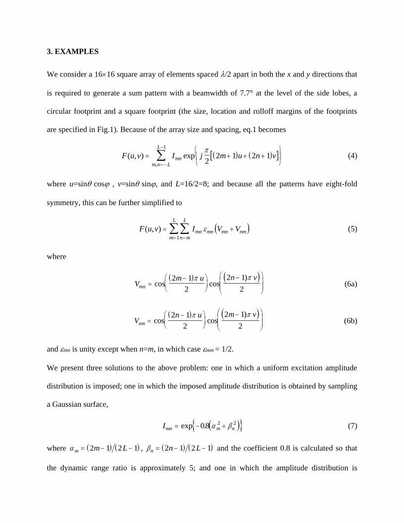
3. EXAMPLES

We consider a 1616 square array of elements spaced /2 apart in both the x and y directions that

is required to generate a sum pattern with a beamwidth of 7.7° at the level of the side lobes, a

circular footprint and a square footprint (the size, location and rolloff margins of the footprints

are specified in Fig.1). Because of the array size and spacing, eq.1 becomes

F u v I j m u n vmnm n L

L

( , ) exp,

22 1 2 1

1

(4)

where u=sin cos , v=sin sin, and L=16/2=8; and because all the patterns have eight-fold

symmetry, this can be further simplified to

F u v I V Vmn mn mn nmn m

L

m

L

( , )

1

(5)

where

V

m u n vmn

cos cos

)2 1

2

2 1

2

(6a)

V

n u m vnm

cos cos

)2 1

2

2 1

2

(6b)

and mn is unity except when n=m, in which case mm = 1/2.

We present three solutions to the above problem: one in which a uniform excitation amplitude

distribution is imposed; one in which the imposed amplitude distribution is obtained by sampling

a Gaussian surface,

Imn m n exp .08 2 2 (7)

where m m L 2 1 2 1 , n n L 2 1 2 1 and the coefficient 0.8 is calculated so that

the dynamic range ratio is approximately 5; and one in which the amplitude distribution is

optimized jointly with the three phase distributions subject only to the condition that the dynamic

range ratio must be less than 20. The first two solutions were obtained using eq.2 for the cost

functions (with the ripple term omitted for the sum patterns), and the third using eq.3 with

C b DRR DRRd' 2. For each condition on the excitation amplitude distribution, the maximum

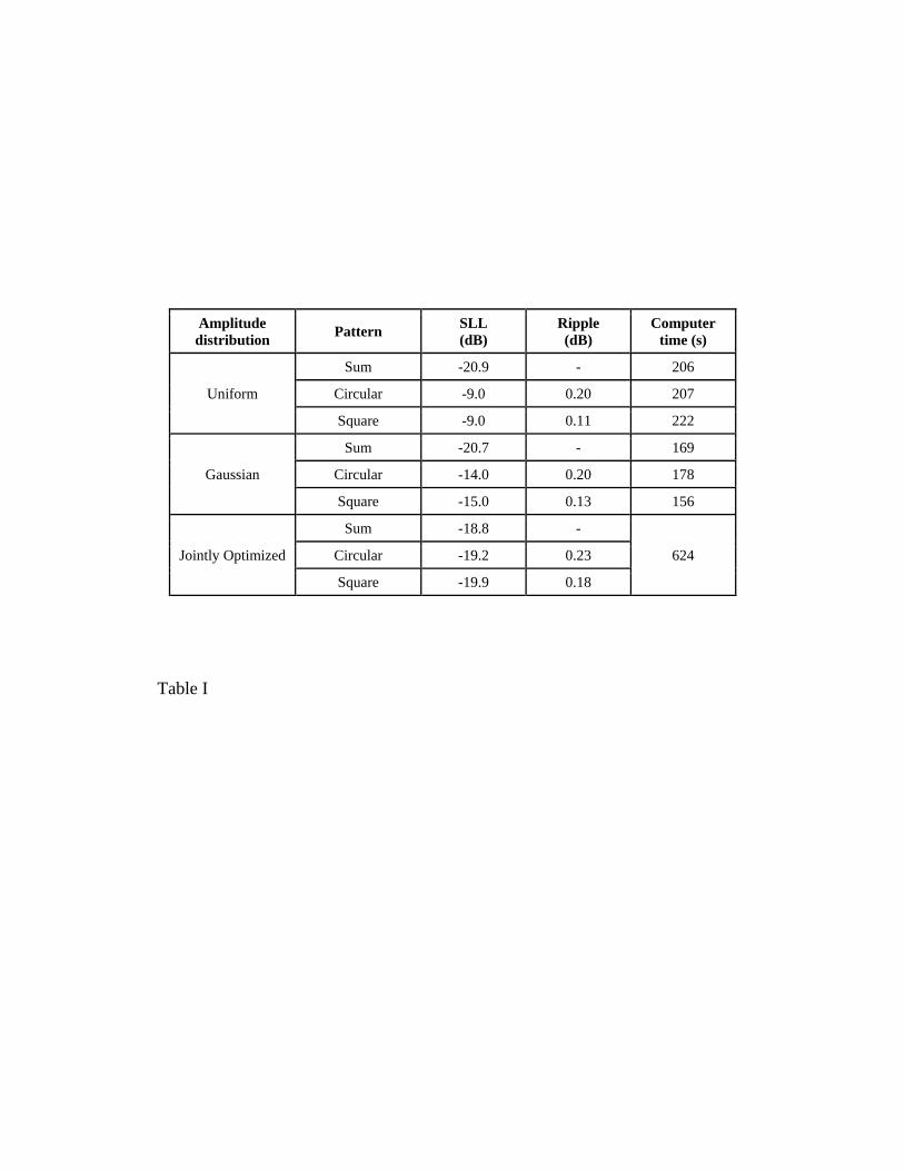
sidelobe and ripple levels of the three patterns are listed in Table I (the ripple values are half the

peak-to-trough differences), together with the time taken to obtain the solution using a computer

with an AMD-K6-2 processor operating at 500 MHz.

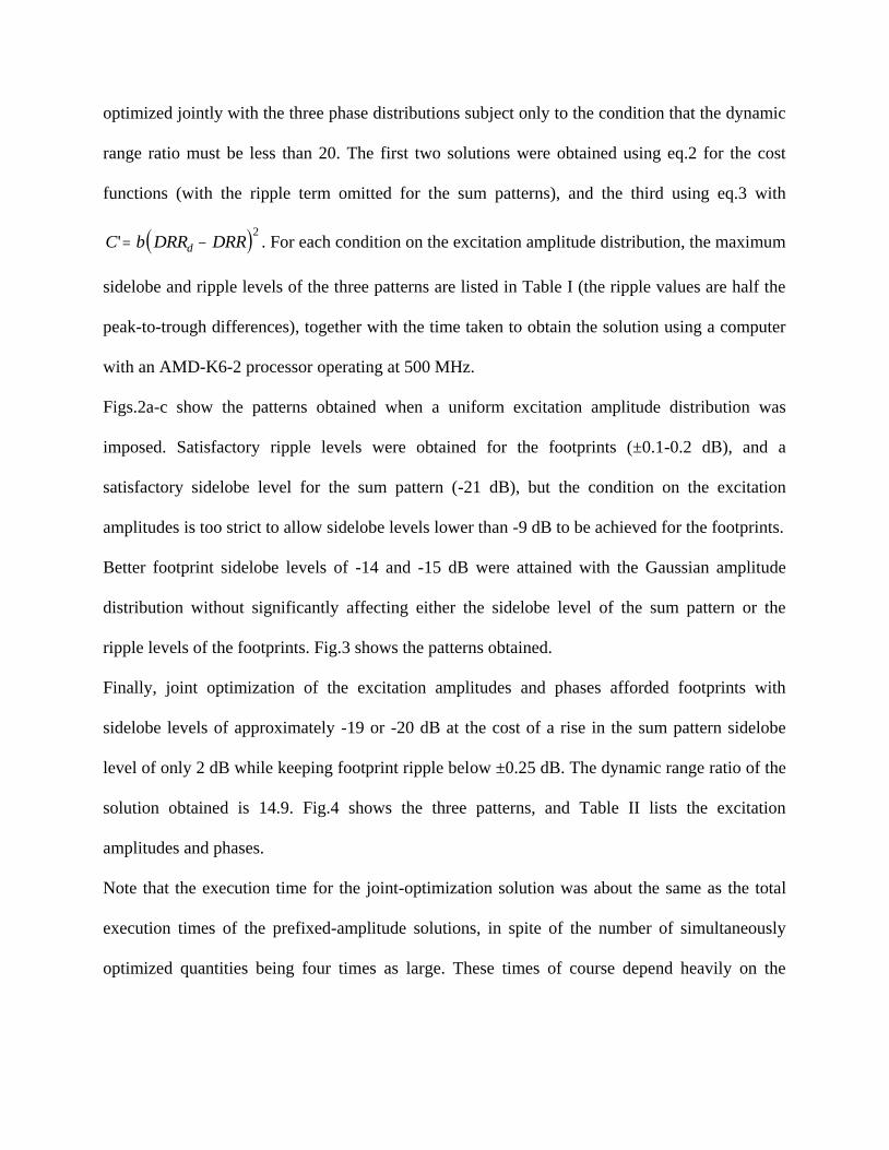
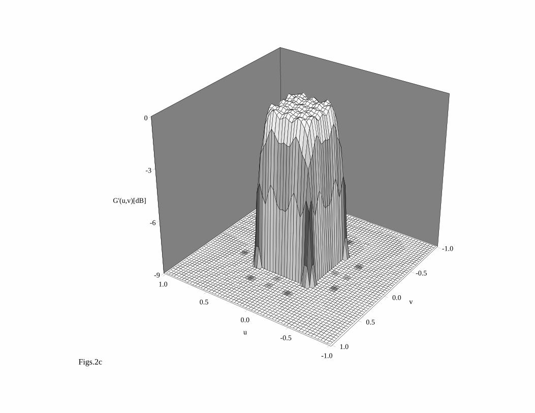
Figs.2a-c show the patterns obtained when a uniform excitation amplitude distribution was

imposed. Satisfactory ripple levels were obtained for the footprints (±0.1-0.2 dB), and a

satisfactory sidelobe level for the sum pattern (-21 dB), but the condition on the excitation

amplitudes is too strict to allow sidelobe levels lower than -9 dB to be achieved for the footprints.

Better footprint sidelobe levels of -14 and -15 dB were attained with the Gaussian amplitude

distribution without significantly affecting either the sidelobe level of the sum pattern or the

ripple levels of the footprints. Fig.3 shows the patterns obtained.

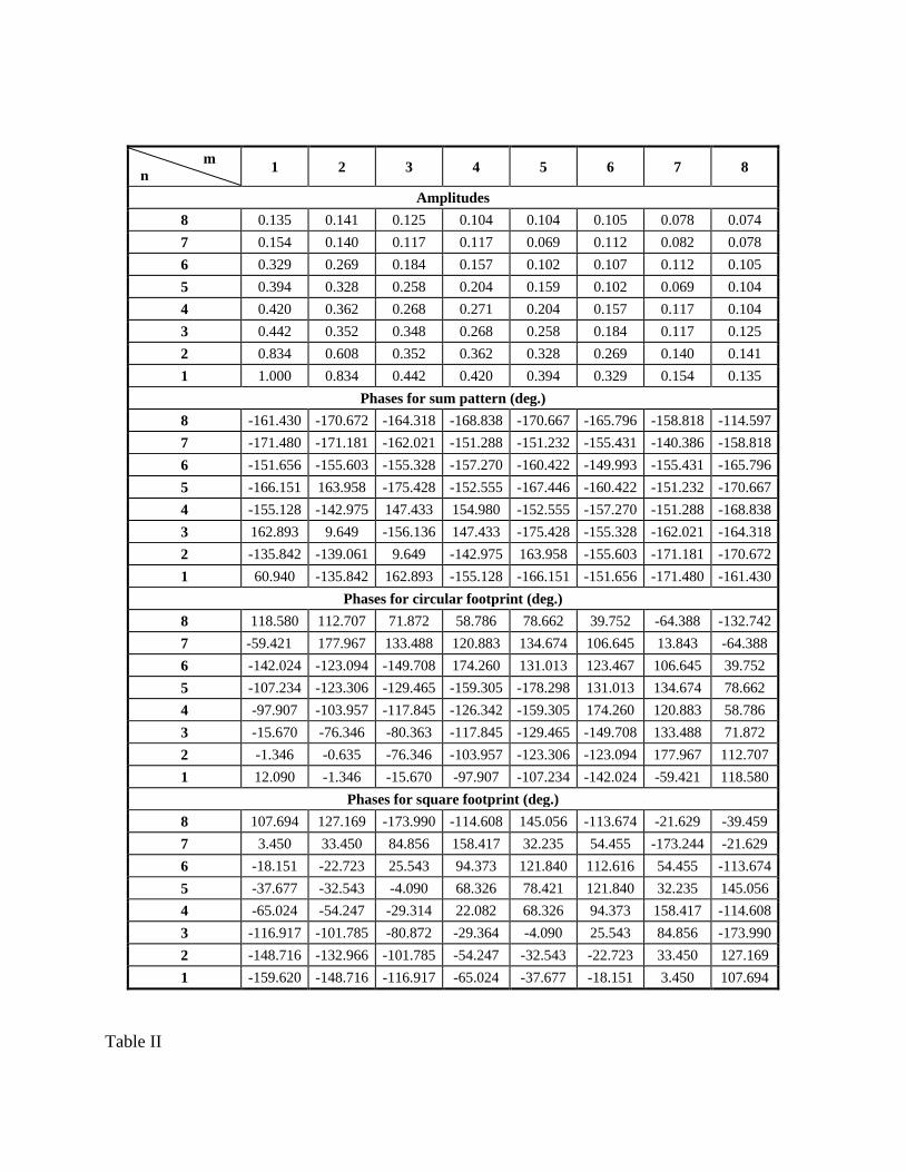
Finally, joint optimization of the excitation amplitudes and phases afforded footprints with

sidelobe levels of approximately -19 or -20 dB at the cost of a rise in the sum pattern sidelobe

level of only 2 dB while keeping footprint ripple below ±0.25 dB. The dynamic range ratio of the

solution obtained is 14.9. Fig.4 shows the three patterns, and Table II lists the excitation

amplitudes and phases.

Note that the execution time for the joint-optimization solution was about the same as the total

execution times of the prefixed-amplitude solutions, in spite of the number of simultaneously

optimized quantities being four times as large. These times of course depend heavily on the

number of points at which the pattern is calculated; in this work the pattern was calculated on a

grid of 6060 points in the (u,v) plane.

4. CONCLUSIONS

Simulated annealing can achieve the synthesis of multi-pattern planar arrays with fixed excitation

amplitude distributions. The amplitude distribution may be prefixed, or optimized jointly with the

pattern-specific phase distributions subject to appropriate smoothness constraints. Computations

can be carried out within reasonable times on conventional desktop computers.

Acknowledgement. This work was supported by the Xunta de Galicia under project

PGIDT00PXI20603PR

REFERENCES

1. M. Dürr, A. Trastoy, and F. Ares, Multiple pattern linear antenna arrays with single prefixed

amplitude distributions: modified Woodward-Lawson synthesis, Electronics Letters, Vol. 36, No.

16, (2000), 1345-1346.

2. X. Díaz, J. A. Rodríguez, F. Ares and E. Moreno, Design of phase-differentiated multiple-

pattern antenna arrays, Microwave and Optical Tecnology Letters, Vol. 26, No. 1, (2000), 53-54.

3. O. M. Bucci, G. Mazzarella, and G. Panariello, Reconfigurable Arrays by Phase-Only Control,

IEEE Trans. Antennas Propagat., Vol. 39, No. 7, (1991), 919-925.

4. W. H. Press, S. A. Teukolsky, W. T. Vetterling and B. P. Flannery, Numerical Recipes in C,

Cambridge University Press, (1992), 444-455.

LEGENDS FOR TABLES

Table I. Sidelobe levels, ripple (half peak-to-trough distance) and computation times of each

pattern obtained under each condition on the excitation amplitude distribution.

Table II. Jointly optimized excitation amplitudes and phases for the three patterns (one quadrant

of the array is shown).

LEGENDS FOR FIGURES

Fig.1. Boundaries defining the base and top perimeters of the circular (a) and square (b)

footprint patterns.

Fig.2. Sum (a), circular footprint (b) and square footprint (c) patterns obtained imposing a

uniform excitation amplitude distribution. G'(u,v) = 20 log(|F(u,v)|/|F(u,v)|max).

Fig.3. As for Fig.2, but for a Gaussian excitation amplitude distribution.

Fig.4. As for Fig.2, but with an excitation amplitude distribution optimized jointly with the three

excitation phase distributions.

Amplitude

distribution Pattern

SLL

(dB)

Ripple

(dB)

Computer

time (s)

Uniform

Sum -20.9 - 206

Circular -9.0 0.20 207

Square -9.0 0.11 222

Gaussian

Sum -20.7 - 169

Circular -14.0 0.20 178

Square -15.0 0.13 156

Jointly Optimized

Sum -18.8 -

624 Circular -19.2 0.23

Square -19.9 0.18

Table I

m

n 1 2 3 4 5 6 7 8

Amplitudes

8 0.135 0.141 0.125 0.104 0.104 0.105 0.078 0.074

7 0.154 0.140 0.117 0.117 0.069 0.112 0.082 0.078

6 0.329 0.269 0.184 0.157 0.102 0.107 0.112 0.105

5 0.394 0.328 0.258 0.204 0.159 0.102 0.069 0.104

4 0.420 0.362 0.268 0.271 0.204 0.157 0.117 0.104

3 0.442 0.352 0.348 0.268 0.258 0.184 0.117 0.125

2 0.834 0.608 0.352 0.362 0.328 0.269 0.140 0.141

1 1.000 0.834 0.442 0.420 0.394 0.329 0.154 0.135

Phases for sum pattern (deg.)

8 -161.430 -170.672 -164.318 -168.838 -170.667 -165.796 -158.818 -114.597

7 -171.480 -171.181 -162.021 -151.288 -151.232 -155.431 -140.386 -158.818

6 -151.656 -155.603 -155.328 -157.270 -160.422 -149.993 -155.431 -165.796

5 -166.151 163.958 -175.428 -152.555 -167.446 -160.422 -151.232 -170.667

4 -155.128 -142.975 147.433 154.980 -152.555 -157.270 -151.288 -168.838

3 162.893 9.649 -156.136 147.433 -175.428 -155.328 -162.021 -164.318

2 -135.842 -139.061 9.649 -142.975 163.958 -155.603 -171.181 -170.672

1 60.940 -135.842 162.893 -155.128 -166.151 -151.656 -171.480 -161.430

Phases for circular footprint (deg.)

8 118.580 112.707 71.872 58.786 78.662 39.752 -64.388 -132.742

7 -59.421 177.967 133.488 120.883 134.674 106.645 13.843 -64.388

6 -142.024 -123.094 -149.708 174.260 131.013 123.467 106.645 39.752

5 -107.234 -123.306 -129.465 -159.305 -178.298 131.013 134.674 78.662

4 -97.907 -103.957 -117.845 -126.342 -159.305 174.260 120.883 58.786

3 -15.670 -76.346 -80.363 -117.845 -129.465 -149.708 133.488 71.872

2 -1.346 -0.635 -76.346 -103.957 -123.306 -123.094 177.967 112.707

1 12.090 -1.346 -15.670 -97.907 -107.234 -142.024 -59.421 118.580

Phases for square footprint (deg.)

8 107.694 127.169 -173.990 -114.608 145.056 -113.674 -21.629 -39.459

7 3.450 33.450 84.856 158.417 32.235 54.455 -173.244 -21.629

6 -18.151 -22.723 25.543 94.373 121.840 112.616 54.455 -113.674

5 -37.677 -32.543 -4.090 68.326 78.421 121.840 32.235 145.056

4 -65.024 -54.247 -29.314 22.082 68.326 94.373 158.417 -114.608

3 -116.917 -101.785 -80.872 -29.364 -4.090 25.543 84.856 -173.990

2 -148.716 -132.966 -101.785 -54.247 -32.543 -22.723 33.450 127.169

1 -159.620 -148.716 -116.917 -65.024 -37.677 -18.151 3.450 107.694

Table II

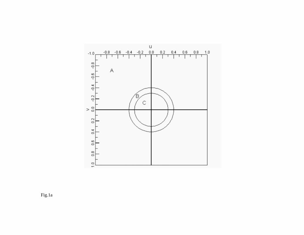
Fig.1a

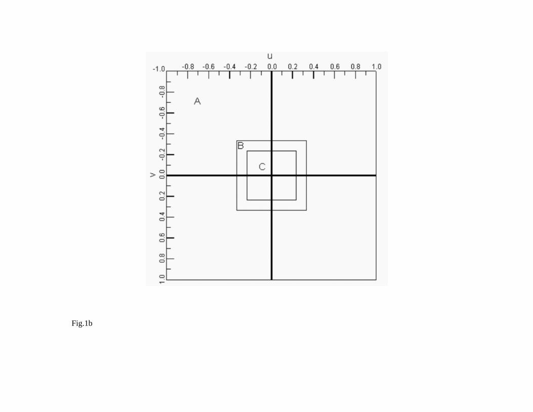
Fig.1b

Fig 2a.-1.0

-0.6

-0.2

0.2

0.6

1.0

u

-1.0

-0.5

0.0

0.5

1.0

v

-20

-15

-10

-5

0

G'(u,v)[dB]

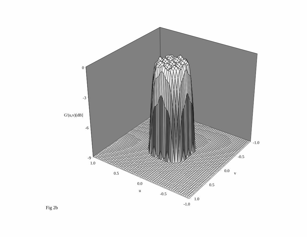
Fig 2b-1.0

-0.5

0.0

0.5

1.0

u

-1.0

-0.5

0.0

0.5

1.0

v

-9

-6

-3

0

G'(u,v)[dB]

Figs.2c-1.0

-0.5

0.0

0.5

1.0

u

-1.0

-0.5

0.0

0.5

1.0

v

-9

-6

-3

0

G'(u,v)[dB]

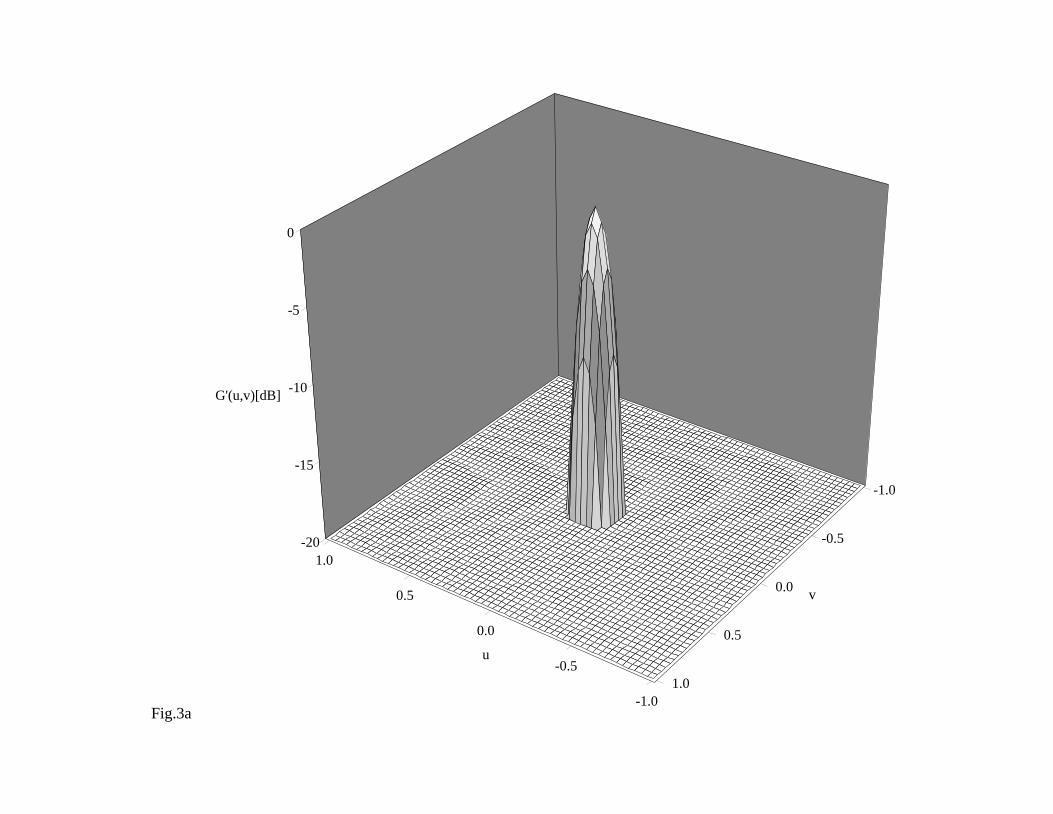
Fig.3a-1.0

-0.5

0.0

0.5

1.0

u

-1.0

-0.5

0.0

0.5

1.0

v

-20

-15

-10

-5

0

G'(u,v)[dB]

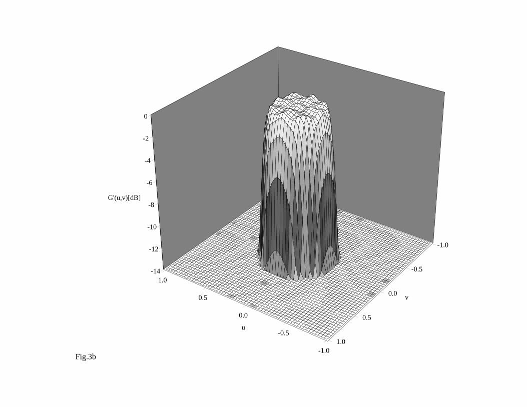
Fig.3b-1.0

-0.5

0.0

0.5

1.0

u

-1.0

-0.5

0.0

0.5

1.0

v

-14

-12

-10

-8

-6

-4

-2

0

G'(u,v)[dB]

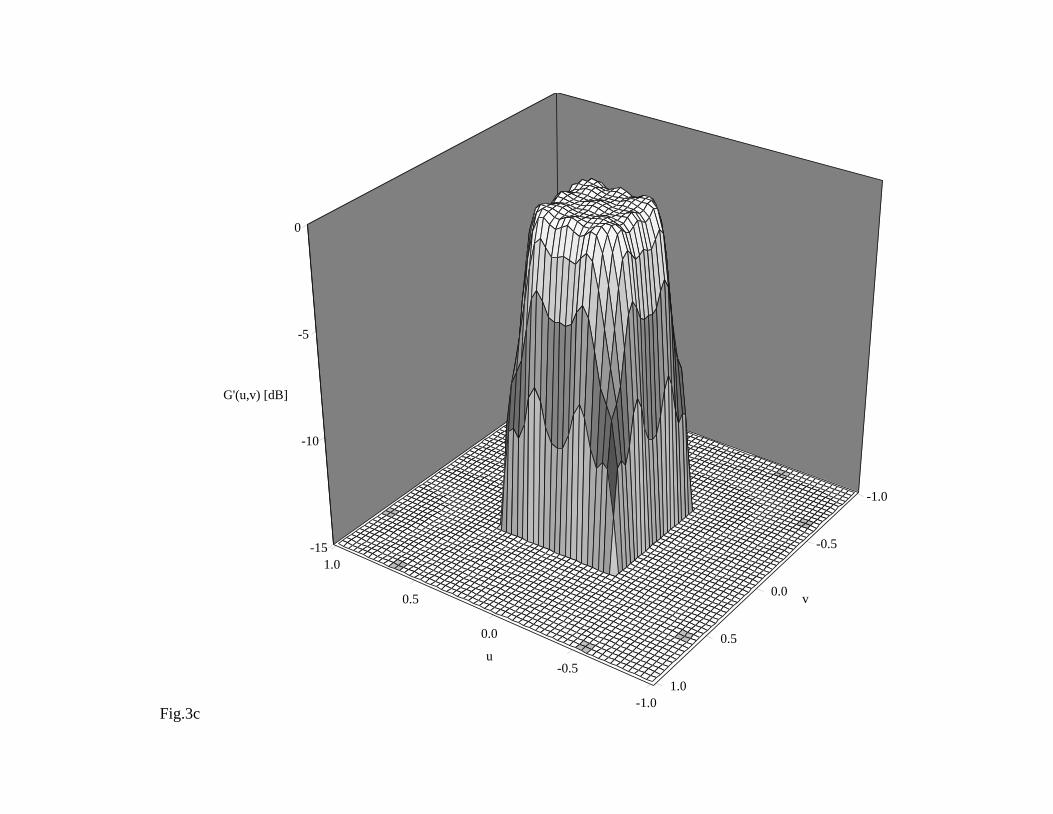
Fig.3c-1.0

-0.5

0.0

0.5

1.0

u

-1.0

-0.5

0.0

0.5

1.0

v

-15

-10

-5

0

G'(u,v) [dB]

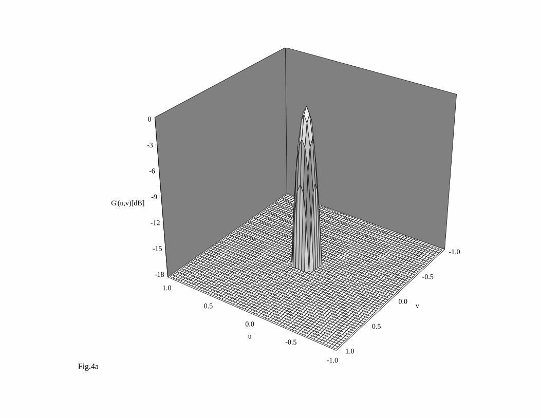
Fig.4a-1.0

-0.5

0.0

0.5

1.0

u

-1.0

-0.5

0.0

0.5

1.0

v

-18

-15

-12

-9

-6

-3

0

G'(u,v)[dB]

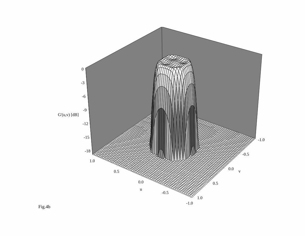
Fig.4b-1.0

-0.5

0.0

0.5

1.0

u

-1.0

-0.5

0.0

0.5

1.0

v

-18

-15

-12

-9

-6

-3

0

G'(u,v) [dB]

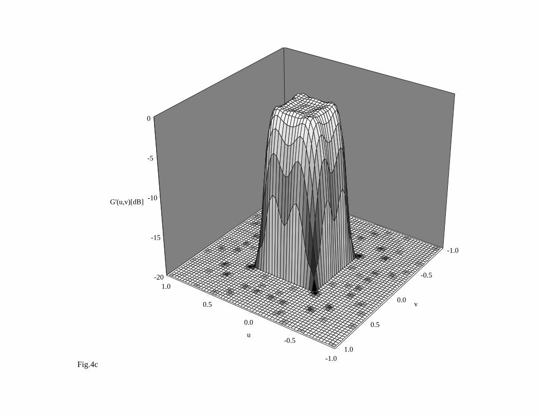
Fig.4c-1.0

-0.5

0.0

0.5

1.0

u

-1.0

-0.5

0.0

0.5

1.0

v

-20

-15

-10

-5

0

G'(u,v)[dB]