Vol. 10, No. 9/September 1993/J. Opt. Soc. Am. A 1953

Synthesis and analysis of planar optical waveguides withprescribed TM modes

Lakshman S. Tamil and Yun Lin

Erik Jonsson School of Engineering and Computer Science and Center for Applied Optics,

University of Texas at Dallas, Box 830688, Richardson, Texas 75083-0688

Received August 31, 1992; revised manuscript received March 9, 1993; accepted March 17, 1993

An inverse-scattering approach to designing optical waveguides with prescribed propagation characteristics of

TM modes is presented. The refractive-index profile of the waveguide is formulated as a solution to a nonlinear

differential equation whose forcing function is the potential obtained from the application of inverse-scattering

theory. This method can reconstruct smooth refractive-index profiles for planar waveguides that support

single modes or multimodes. The cases of both zero and nonzero reflection coefficients characterizing the

transmission properties of waveguides are discussed. A direct analysis technique based on a finite-difference

scheme has been formulated to verify the results obtained by the inverse-scattering method, and the twoapproaches are in excellent agreement.

1. INTRODUCTION

The conventional method of designing optical waveguidingstructures is to assume a refractive-index profile and solvethe governing differential equation to find the variouspropagating modes and their propagation characteristics.If the propagation characteristics do not exhibit the ex-pected behavior, the refractive index is changed and thepropagation characteristics are again evaluated; this isrepeated until the expected propagation behavior of themodes is obtained. Since the procedure is iterative, it istime consuming. Also, to obtain certain arbitrary trans-mission characteristics, one may not be able to guess thecorrect initial refractive-index profile. One normallythinks of initial profiles that have a mathematically closedform, such as parabolic and secant hyperbolic.

The procedure discussed in this paper, as opposed tothe direct method, starts with the required propagationcharacteristics of the waveguide and obtains the refractive-index profile as the end result. We achieve this by trans-forming the wave equation for both the TE and the TMmodes in the planar waveguide to a Schrodinger-type equa-tion and then applying the inverse-scattering theory asformulated by Gel'fand and Levitan' and by Marchenko.2

The inverse-scattering problem encountered here has a di-rect analogy to the inverse-scattering problem of quantummechanics. The refractive-index profile of the planarwaveguide is contained in the potential of the Schr6dinger-type equation, and the propagating modes are the boundstates of quantum mechanics.3

An inverse-scattering theory with a zero reflectioncoefficient characterizing the propagation property wasapplied by Yukon and Bendow to the design of planar wave-guides.4 In that investigation the refractive-index pro-files were constructed only for the prescribed TE modes.The inverse problem of designing optical waveguideswhose transmission property is characterized by a nonzeroreflection coefficient was solved for TE modes by Jordanand Lakshmanasamy.5 In this paper we have applied theinverse-scattering theory with both the zero and the non-

zero reflection coefficients to design planar waveguideswith prescribed TM modes.

In Section 2 we review the problem of electromagneticwave propagation in a planar waveguide for both TE andTM cases,6 then we present a way to transform wave equa-

tions into Schrodinger-type equations. In Section 3 wereview Kay's inverse-scattering theory7 and the Gel'fand-Levitan-Marchenko equation.12 Inverse-scattering the-ory is then applied to planar waveguides for the case of TMmodes in the zero and the nonzero reflection-coefficientconditions separately. We obtain the single-mode and themultimode refractive-index profiles with prescribed TMmodes by solving a nonlinear differential equation, usingthe Runge-Kutta fourth-order approximation method, asdiscussed in Sections 4 and 5. In Section 5 we presentthe construction of the potentials for a single-mode planarwaveguide for the nonzero reflection-coefficient case,using a rational function of wave number to obtain ref lec-tion coefficients.

To verify the results obtained by inverse-scatteringtheory, we have developed an efficient finite-differencemethod to find the propagation constants of guided TEand TM modes, and we present the method in Section 6.We start from the wave equations for TE and TM modesand transform them into a set of finite-difference equa-tions. Then a matrix eigenvalue equation, from whichthe propagation constants can be found, is constructed.The numerical results are obtained for several graded-index waveguides, and we compare these results with pre-viously published analytical solutions and results obtainedby other numerical methods. The conclusions are givenin Section 7.

2. PHYSICAL MODEL OF A PLANARWAVEGUIDE

The wave equations for inhomogeneous planar opticalwaveguides can be derived from Maxwell's equations. Ifwe take z as the propagation direction and let to repre-sent the frequency of laser radiation, we have the follow-

0740-3232/93/091953-10$06.00 © 1993 Optical Society of America

L. S. Tamil and Y Lin

1954 J. Opt. Soc. Am. A/Vol. 10, No. 9/September 1993

e^ n~ikx

r(k) e

_ CORE\-n2

0 d

Fig. 1. Physical structure of the inhomogeneous symmetricalplanar optical waveguide, showing reflection and transmission ofan electromagnetic wave.

ing wave equations for one-dimensional inhomogeneousplanar waveguides6 :

We now need to transfer the wave equation for the TMmodes into a Schrddinger-type equation to apply theinverse-scattering method. In Eq. (2) the first derivativeof EX can be eliminated if we let E.(x) = e

2 (x)D(x).The wave equation then becomes

d( 2 1 d2 e(x) 3 [de(x) 1dx2 2e(x) dx2 4e2 (x) [ dx J

+ [o 2e(x) - 32]( = 0. (6)

We are now able to obtain the equivalent Schrodingerequation,

d '((x) + [k2 - V(x)]@b(x) = 0, (7)dX2

by setting the potential function as

3 [de(X) 2 1 d2 ,E(X) 2V(x) =4e(x) [ dx 2e(x) dx - ko2[e(x) - n.

(8)

and letting

2 = 2= k02n 2

- ,l2.

_X2EY(X) + [ko2 e(x) - p 2]E,(x) = 0 (1)

(9)

for TE modes and

d2 d Fi de(x) 1dX2Ex(x) + dx [e(x) dx E JW

+ Eko2e(x) - p32]E.(x) = (2)

for TM modes. The planar waveguide that we are consid-ering here has a refractive index that varies continuouslyin the x direction. For the planar optical waveguideshown in Fig. 1, our problem is to find the refractive-indexprofile function in the core for a set of prescribed propaga-tion constants.

We assume that this planar waveguide has a refractive-index profile guiding N modes. The propagation con-stants {n} are kon > 1 > 82 > ... ,BfN Ž kon,,, in whichn,. is the value of n(x) as x --. - and n = sup n(x). Thedesign of an optical waveguide is analogous to the inverseproblem encountered in quantum mechanics. We are,in effect, trying to obtain the potential function from thegiven bound states and scattering data. The wave equa-tion for the TE modes can be easily transformed into anequivalent Schr6dinger equation,

-XE,(x) + [k2 - V(x)]E,(x) = 0, (3)

by letting

V(x) = -k02 [n2 (x) - n 2], (4)

k2 = K K 2 = Q 3(2 - k 2n , 2). (5)

We can see that in our case the potential function V(x) iscontinuous and V(x) - 0 as x - -. The TE mode caseshave been solved by Yukon and Bendow4 and Jordan andLakshmanasamy,5 and so our discussion will be restrictedto TM modes.

3. INVERSE-SCATTERING THEORYThe inverse-scattering theory of Kay and Moses8 providesa way to obtain the potential from the reflection coeffi-cient that characterizes the propagation properties of theplanar waveguide. As the potential that we defined van-ishes at infinity, we can apply the Gel'fand-Levitan-Marchenko equation to solve our problem. Let us considera time-dependent formulation of the scattering. We takethe Fourier transform of Eq. (7) [the transform pairs areF(x, k) '= P(x, t) and k '- t to obtain

a2 a2

-X 2(X, t) - -'I'(xt) - V(x)T(x,t) = 0, (10)

in which t is the time variable, with the velocity of lightc -1. The incident plane wave is represented by theunit impulse

P(x,t) = 8(x - t), x < 0, t < 0, (11)

which produces the reflected transient wave function

R(x + t) =-f r(k)exp[-ik(x + t)]dk2 7r _.

N

+ lAn exp[-iKn(x + t)], (12)n-l

where k =-Kn 2 are the discrete eigenvalues of theSchrodinger-type equation [Eq. (7)], r(k) is the complexreflection coefficient, and An are arbitrary constants nor-malizing the wave equation such that

f ) (x)bl*(x)dx = 1. (13)

The reflected transient is produced only after the inci-dent unit impulse has interacted with the inhomogeneous

L. S. Tamil and Y. Lin

Vol. 10, No. 9/September 1993/J. Opt. Soc. Am. A 1955

core of the optical waveguide, and therefore

R(x + t) = 0 for x + t c 0. (14)

A linear transform independent of k can now relate thewave amplitude P(x, t) in the core region with the waveamplitude To(x, t) in the exterior region:

I'(X, t) 'Po(x, t) + J K(x, 6')%(' t)d6' x > 0.

to(X, fxi i (15)

Here the exterior field is

To(x,t) = 8(x - t) + R(x + t). (16)

equations for fn(x):

An E {expiKv K) }f" (x) + f(x) + A. exp(Knx) = 0,

(23)

where n = 1, 2,... N. This system can be convenientlywritten as

Af + B =0, (24)

where f and B are column vectors with fn and Bn =

An exp(Knx), respectively, and A is a square matrix withelements

From physical consideration, since 'I(x, t) is a rightward-moving transient,

T(x, t) = 0 for t < x . (17)

Thus the kernel K(x, t) = 0 for t > x and K(x, t) = 0 fort c -x. We substitute Eq. (16) into Eqs. (15) and useEqs. (14) and (17) to obtain the integral equation

K(x,t) + R(x + t) + L K(x,6')R({' + t)d' = 0,

A = 6wn + A {exp[(KvKn)X]vn v ~Kv + Kn

(25)

in which 5,n is a Kronecker delta. The solution for f isf = -A7'B, and from Eq. (22) K(x, x) = ETf, where E is acolumn vector with element En = exp(Knx) and T denotestranspose. Now

d Avn = A,, exp[(K, + KJ)X] = BnEn, (26)

t < x. (18) and so

By substituting Eqs. (15) into Eq. (10), we can show t

the kernel K(x, t) satisfies a differential equation ofsame form as Eq. (10), provided that the following cotions are imposed:

K(x,-x) = 0,d2-K(x, x) = V(x).

dx

We can now see how the solution of the integral Eq.for the function K(x, t) can lead to the synthesis of optwaveguides.

4. DESIGN EXAMPLE 1: ZEROREFLECTION COEFFICIENT

The reflection coefficient characterizes the propagaproperties of optical waveguides. A zero reflection coi

cient characterizes a system with propagating modes cwhereas a nonzero reflection coefficient characterizsystem with both guided and unguided modes. Lefirst consider the special case of a zero reflection cocient. 8 We substitute Eq. (12) for r(k) = 0 in the Gel'fELevitan-Marchenko equation [Eq. (18)] to obtain

NK(x, t) + >, An exp[Kn(x + t)]

n-1

+ NAnf K(x,6)exp[Kn(t + 6)d6 = 0.n-1 -

It is clear from Eq. (21) that the solution for K(x, t) sbhave the form8

NK(x, t) = f f,(x)exp(Knt).

n=1

dK(x, x) = E~fn = -EnA,,j'B = .'A,

dx(27)

when written with subscript notation and the summationconvention. The K(x, x) given by Eq. (22) can be recog-nized in the form

K(x, x) = tr(A ) = d ln(det A), (28)

and therefore the potential V(x), according to Eq. (20), is

V(x) = -2 dX2 ln(det A) . (29)

Given N modes with desired propagation constants, wecan obtain a potential function as given by Eq. (29). Herewe have N degrees of freedom that are due to N arbitraryconstants {An I n = 1, 2,... N}.

For TE modes the refractive-index profile is simplygiven by

n2(X) = n 2- V(x), (30)

in which ko is the free-space wave number. For TM modesobtaining the refractive-index profile is more complicatedbecause it is a solution to a nonlinear differential equation

(21) [Eq. (8)]. The nonlinear differential equation can besolved only numerically. First we transform Eq. (8) into

ould a convenient form by setting e(x) = exp[y(x)]. We thenobtain

1 d 2y (x)_ 1 dyX 2(22) 2 X

2 4 xJ+ ko exp[y(x)]

We substitute Eq. (22) into Eq. (21) to produce a system of

L. S. Tamil and Y. Lin

2+ [V(x - ko n2l = 0 - 31)

1956 J. Opt. Soc. Am. A/Vol. 10, No. 9/September 1993

2.205

X0

4)

C4

(m)

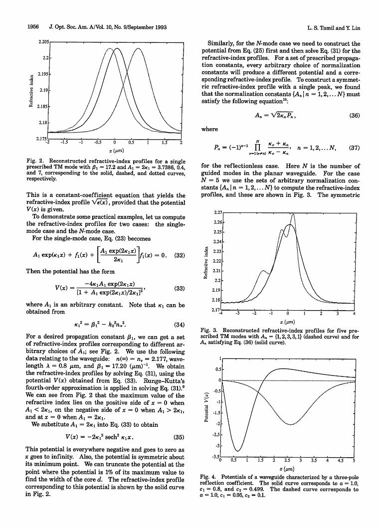
Fig. 2. Reconstructed refractive-index profiles for a singleprescribed TM mode with ,1 = 17.2 and Al = 2KI = 3.7386, 0.4,and 7, corresponding to the solid, dashed, and dotted curves,respectively.

This is a constant-coefficient equation that yields therefractive-index profile \/I , provided that the potentialV(x) is given.

To demonstrate some practical examples, let us computethe refractive-index profiles for two cases: the single-mode case and the N-mode case.

For the single-mode case, Eq. (23) becomes

Similarly, for the N-mode case we need to construct thepotential from Eq. (25) first and then solve Eq. (31) for therefractive-index profiles. For a set of prescribed propaga-tion constants, every arbitrary choice of normalizationconstants will produce a different potential and a corre-sponding refractive-index profile. To construct a symmet-ric refractive-index profile with a single peak, we foundthat the normalization constants {An I n = 1, 2 . . . N} mustsatisfy the following equation":

(36)

where

N K + KnH

v-1('#n) Kv -Kn(37)

for the reflectionless case. Here N is the number ofguided modes in the planar waveguide. For the caseN = 5 we use the sets of arbitrary normalization con-stants {An I n = 1, 2... N} to compute the refractive-indexprofiles, and these are shown in Fig. 3. The symmetric

Al exp(KIx) + f(x) + [A 1 exp(2KCX) = 2K, f()OThen the potential has the form

VWx = -4K 1 Aj exp(2Klx)[1 + Al exp(2Kx)/2Kj]2

(32)

(33)

where Al is an arbitrary constant. Note that K can beobtained from

K12 = P12 - k 2n2. (34)

For a desired propagation constant j,1, we can get a setof refractive-index profiles corresponding to different ar-bitrary choices of Al; see Fig. 2. We use the followingdata relating to the waveguide: n(-) = n = 2.177, wave-length A = 0.8 m, and , = 17.20 (m)-'. We obtainthe refractive-index profiles by solving Eq. (31), using thepotential V(x) obtained from Eq. (33). Runge-Kutta'sfourth-order approximation is applied in solving Eq. (31).9We can see from Fig. 2 that the maximum value of therefractive index lies on the positive side of x = 0 whenAl < 21, on the negative side of x = 0 when Al > 2

KI,

and at x = 0 when A, = 2K1.

We substitute Al = 21 into Eq. (33) to obtain

V(x) = -2K12 sech2KjX.

(m)

Fig. 3. Reconstructed refractive-index profiles for five pre-scribed TM modes with An = {1, 2,3,3, 1} (dashed curve) and forAn satisfying Eq. (36) (solid curve).

X (m)Fig. 4. Potentials of a waveguide characterized by a three-polereflection coefficient. The solid curve corresponds to a = 1.0,c = 0.8, and 2 = 0.499. The dashed curve corresponds toa = 1.0, cl = 0.05, 2 = 0.1.

q

00..

(35)

This potential is everywhere negative and goes to zero asx goes to infinity. Also, the potential is symmetric aboutits minimum point. We can truncate the potential at thepoint where the potential is 1% of its maximum value tofind the width of the core d. The refractive-index profilecorresponding to this potential is shown by the solid curvein Fig. 2.

C)0

S)

C)

L. S. Tamil and Y. Lin

An = 'V2--KnP.,

P = (-1)n-

Vol. 10, No. 9/September 1993/J. Opt. Soc. Am. A 1957

profile obtained from Eq. (36) is shown by the solid curvein the figure.

5. DESIGN EXAMPLE 2: NONZEROREFLECTION COEFFICIENT

In Section 4 we took advantage of the fact that the reflec-tion coefficient was zero, which simplified the problemconsiderably. Now we are going to solve the problem with

a nonzero reflection coefficient. We follow the work ofJordan and Lakshmanasamy. 5

We take the rational-function approximation for ourscattering data. We represent our reflection coefficientby using a three-pole rational function of transverse wavenumber k5. One pole lies on the upper imaginary axis ofthe complex k plane, which represents a discrete spectrumof the function R(x + t) [Eq. (12)] characterizing thepropagating mode. Two symmetric poles lie in the lower

half of the k plane, which represent the continuous spec-trum of R(x + t) characterizing the unguided modes.The three-pole reflection coefficient can be written as

(k - kD(k - k2)(k - k 3)(38)

where r can be determined by the normalization condi-tion r(O) = -1, which ensures total reflection at k = 0.k1 and k2 have the following forms: k = -c 1 - ic 2 andk2 = C1 - ic 2 . The third pole on the positive imaginaryaxis is k 3 = ia.

The pole positions are confined to certain allowed re-gions that are determined by the law of conservation ofenergy, which can be represented by Ir(k)12 c 1 for all realk; see Fig. 3 of Ref. 5 for details.

It has been shown that the reconstructed potential func-tion V(x) has the following form:

[ d[a T(X)] rx)lx d[A(x)]11V) = 2 [dx - aT(x)Ad(x)dx 1A-l(x)b, (39)

in which a and b are column vectors and are given by

aT(x)

= [1 x exp(71lx) exp(-q 1lx) exp(712x) exp(-'q 2x)],(40)

bT = [0 0 0 0 0 -a(c, 2 + c22 )], (41

where

71l = [/2a 2+ C2

2 - 12 + /2(a2 - 4C22 )12 (a2 + 4c2)1/2il/2,

(42

712 [2a 2 + 22 - C1

2 - 1/2 (a2 - 4C22)1/2(a2 + 4c1

2)1 2]11 2.(43

Matrix A(x) is given by

2.184-

2.182 -

2.18

2.178

2.176-

2.17410 0.5 1 1.5 2 2.5 3 3.5 4 4.5 5

(Am)

Fig. 5. Reconstructed refractive-index profiles corresponding tothe potentials shown in Fig. 4.

where

f(x) = x3 + (2c2 - a)x 2

+ (C12 + C22- 2ac2)x - a(c,2 + C2

2). (45)

So it is possible to construct the potential from thethree poles of the reflection coefficient by means of theabove equations. We choose two examples. In example 1,the poles are determined by the parameters a = 1.0,cl = 0.8, and c2 = 0.499; example 2 has different unguidedmodes characterized by cl = 0.05, c2 = 0.1, and the samepropagating mode characterized by a = 1.0. Figure 4shows the plots of the potential functions for examples 1and 2. In example 2 we see that the potential is negativeeverywhere.

Figure 5 shows the refractive index profiles for the TMmode in both of the examples discussed above obtainedwhen one substitutes the potentials into Eq. (31) and solvesfor \/_Y(x. We note that a depressed cladding is obtainedin example 1, and we also see that the profiles that we findresemble the profiles that we normally find in practicaloptical waveguides. 11

6. VERIFICATION BY ANALYSIS

To verify the results obtained by inverse-scattering theory,a finite-difference based analysis scheme is developedhere. We use this method to find the propagation con-stants of the guided TM modes of an optical waveguidewith an arbitrary refractive-index profile. Owing to itssimplicity and flexibility, this method is proved to beeffective.

We consider a symmetric planar waveguide. For theTM modes we have6

0

f(71')0

exp(-71lx)-711 exp(-71 1 x)

7712 exp(-71lx)

0

a(ci 2 + C22)

0

exp(71lx)

7ql exp(7 1 x)

7112 exp(71x)

0

0

f(712)

exp(-71 2x)

712 exp(-712x)

7122 exp(-'7 2 x)

0 1

0 00 01 -X

O -1

0

0 10

a(c 2 + C22)

exp(-72 x)

712 exp(712X)

7122 exp(71 2 x)

y (44)

L. S. Tamil and Y. Lin

L)I

- . 1. . - -

1958 J. Opt. Soc. Am. A/Vol. 10, No. 9/September 1993

tration (see Fig. 6). For the case considered here theboundary conditions are

Ho = 0,

H8 = 0;

_7 COVER

-6 n2

SUBSTRATEn2

0

Fig. 6. Planar optical waveguide showing grid points in the sub-strate, the film, and the cover.

Ey = Hx = Hz = 0,

E. = (W)Hy,

(- = - ;6) -co ax

with the Hy component obeying the wave equation

2 a 1 ay = [2 _ n2 (X)ko2]H(x)n ax kn ax I()

(46)

(54)

(55)

that is, the field vanishes at the ends of the cladding. Anabsorbing boundary condition would have been more ap-propriate; however, it is not used here.

We can write a finite-difference equation at every gridpoint from i = 1 to i = 7. We use the function f(i) to rep-resent the derivative of n(i) that is obtained again by afinite-difference approximation and is denoted by

- dn(i)dx (56)

(47) Note that f goes to zero in the substrate and in the coverregion. The refractive indices in the substrate and thecover are represented by n, and n, respectively. At i = 1

(48) Ho = 0, and so

(49)

(n,2k,2-2 - W) lH + Hi2 = 0.

At i = 2,

(57)

For the one-dimensional graded-index planar waveguide,the refractive index is a function of x, and the wave equa-tion can be transformed into

h (fl.k-

In the film, at i = 3,

,p2- 2)2 + h3 = 0.

d 2HY(x)_ 2 d[n(x)] dHy(x)dx2 n(x) dx dx

+ [n2(x)k02 - f32]H,(x) = 0. (50)

If Hy and its derivative are single-valued, finite, andcontinuous functions of x, we have the following finite-difference approximations to the differentials:

dH _ Hi+, - Hi-,dx 2h

d2H Hj+1 - 2i + Hi-,dx2 h2

(51)

(52)

in which we have used H instead of Hy for simplicity. Wehave Hi,- = H(x - h), H, = H(x), and Hi+ = H(x + h),in which h is the distance between the grid points and i isthe index of the grid point. We obtain Eq. (53) by substi-tuting the finite-difference approximation of the first andthe second derivatives of H into Eq. (50):

(1 1 dn~ i . + (, 2k2 2"(1+ - - Hi- + ni2kO _ '32 - h2Hih2 nh dx / O 2 I

2 nihdxHi+l = 0, (53)

in which n = n(ih) and the value of dni/dx is the deriva-tive of the refractive index n at x = ih.

We have chosen three grid points in each region: thesubstrate, the film, and the cover, for the purpose of illus-

[1 1 WMf(l) H2 + [2(1)k02 _ ,2 - !llf(1)] ) 4 0 ( 9' h n ( 1 ) h I.'n~ l ~

+ h n(1)h f(1)]li4 = * (59)

At i = 4,

[h + 7(2)h f(2) ]H3 + [fn2(2)k 02 p2- 4

+ [ - n(2)h f(2)]Hs = 0. (60)

At i = 5,[ 1 1 1 2 ]h n(3)h f(3) 4 + [n2(3)k 02 - p2

- 2 H

+ [h n(3)h f(3)]li = 0.

At i = 6,

hH6 + [nc2k02 _ -P2- 1H6 + h2H 7 = 0,

At i = 7, since H8 = 0, we have

I + (f2k02 - - 2 = 0.

(61)

(62)

(63)

For convenience, we can rewrite these finite-differenceequations as a matrix equation:

(58)

L. S. Tamil and Y. Lin

Vol. 10, No. 9/September 1993/J. Opt. Soc. Am. A 1959

2 - P c

a3 2 a33

O

0

o 0 0 0 0

a23 0 0 0 0

- 2 a34 0 0 0

a43 a 4 4 -13 2 a4 5 0 0

0 a54 a 5 5 - 32 a5 6 0

0 0 a6 5 a 6 6 - 2 a6 7

o 0 0 a7 6 a 7 7 - f32

in which the elements of matrix A are defined by

2a12 = -- + n2 k0 = aNN,

1a12 = W = aNN-1

and, for 2 c i < N,

which has a nontrivial solution if and only if 132 are eigen-values of B. So, finally, we have

(65){p} = Veig[Bj (73)

(66) for both odd and even modes. For the TE modes the situ-ation is much easier, since the wave equation has a simplerform than that for the TM modes. The field component E,obeys the wave equation 6

2' icN, N+N2<i<N

(i)h(67)

n|1 k 2-- 2-cicN 1, N+N 2<i<N

n(i)h 2

(68)

|n2 ko2 2 c i-cNi, N + N2< i< N

n Wiko-h N1 < i c N1+N2

(69)

f(i) is the derivative of the refractive index at x = ih; N1 ,N2, and N3 are the number of grid points in the substrate,the film, and the cover, respectively; and N = N1 + N2 +

N3 is the total number of grid points. The other elementsof the matrix that are not defined above are zeros.

The matrix A can now be split into

A = B - p32l, (70)

where I is the identity matrix and the matrix B has thefollowing simple form:

a 1

a 2 1

0

0

0

0

0

a 12 0 0 0 0 0

a2 2 a2 3 0 0 0 0

a3 2 a3 3 a3 4 0 0 0

0 a4 3 a4 4 a4 5 0 0

0 0 a54 a55 a56 0

0 0 0 a65 a6 6 a6 7

O 0 0 0 a76 a7 7

a2E,(x) = [2 - n2(x)k02 ]E,(x).

aX2 (74)

We can find a matrix expression similar to the one wefound for the TM modes. In the TE case we need notcalculate the derivative of the refractive-index profile.

For the given refractive-index profile distributionn = n(x) the matrix B can be constructed and the propa-gation constants {/3} can be obtained by solving for theeigenvalues of this matrix.

Before we attempt to analyze the refractive-index pro-files obtained by the application of inverse-scatteringtheory, we would like to see whether the finite-differencetechnique developed here provides the right result. To dothat, we have applied the technique to various refractive-index profiles, such as parabolic and Gaussian, for whichresults are already available in the literature. 12 The re-sults corresponding to TM modes are given in Tables 1and 2 and show that our analysis technique is accurateand powerful.

Having established the accuracy of the finite-differencetechnique, now we can use this technique on the arbitraryrefractive-index profiles that we have obtained. Figure 7shows the dispersion characteristics for the refractive-index profile with the single symmetric peak shown inFig. 3. The normalized frequency V has been determinedfrom the waveguide thickness and the free-space wave-length of the propagating modes. Here we have V =kod \n2 - n2 = 37.6883. The normalized propagationconstant that we used here is defined by

(13/ko)2 -n22

n 2 -n2(75)

(71)

Equation (64) can now be rewritten in the form

B - /321H = 0. (72)

To find the propagation constants of the guided TMmodes, we must solve the eigenvalue problem of Eq. (72),

Here n2 is the refractive index of the cladding and ni is themaximum refractive index of the core. The number ofTM modes present is the same number that we startedwith in reconstructing the profile. When analyzed, therefractive-index profiles corresponding to the nonzero re-flection coefficient, as shown in Fig. 5, yield the dispersioncharacteristics shown in Fig. 8. Again we see the consis-tency in the number of modes obtained by analysis andthe number of modes used in the synthesis of the profile.

a 12

a2 :

all _ 2

a2 l

0

0

0

AH =

0 0

o 0

'H1

H2H3

H4

H5

H6

= 0, (64)

L. S. Tamil and Y Lin

1960 J. Opt. Soc. Am. A/Vol. 10, No. 9/September 1993

Table 1. Mode Spectra pr/ko (TM) of SymmetricTruncated Parabolic Index Profile of Ag-Diffused

Waveguide with n2 = 1.5125, n, = 1.5991,A = 0.6328 tim, and Thickness d = 9.1400 ,um

ModeNumber I3./ko from fy/ko from Finite-Difference Method

(y) Ref. 12 N2 = 84a N2 = 168-

0 1.5966 1.5966 1.59661 1.5915 1.5915 1.59152 1.5864 1.5864 1.58643 1.5813 1.5813 1.58134 1.5762 1.5762 1.57625 1.5711 1.5711 1.57116 1.5659 1.5658 1.56597 1.5607 1.5604 1.56058 1.5556 1.5546 1.55489 1.5503 1.5498 1.5499

10 1.5451 1.5439 1.544311 1.5399 1.5387 1.539012 1.5346 1.5326 1.533613 1.5294 1.5288 1.529014 1.5241 1.5228 1.523115 1.5188 1.5139 1.5143

aN2 is the number grid points in the core.

7. DISCUSSION AND CONCLUSIONSWe have developed a method based on inverse-scatteringtheory that can be used to design planar optical wave-guides that transmit a prescribed number of TM modeswith prescribed propagation constants. The results havebeen verified by means of finite-difference analysis. Thisprocedure, in conjunction with the technique for design-ing planar optical waveguides for prescribed TE modesdeveloped in Refs. 4 and 5, provides the complete inverse-scattering procedure for designing planar optical wave-guides with prescribed propagation characteristics.However, it should be mentioned that only the character-istics of one kind of mode (TE or TM) can be prescribedin a waveguide, as the two kinds of mode are governed bytwo different differential equations.

One important question that should be answered whenwe fabricate actual waveguides with refractive-index pro-files obtained with the technique described here is withwhat precision the nx) should be fabricated to provide thedesired mode configuration. To answer this question wehave changed V(x) [V(x) is related to n(x) through Eq. (30)]uniformly over the spatial distance x by 1%, 5%, and 10%

Table 2. Mode Spectra p,/ko (TM) of SymmetricTruncated Gaussian Index Profile of Ag'-Diffused

Waveguide with n2 = 1.5125, n = 1.6014,A = 0.6328 ,um, and Thickness d = 9.1700 ,um

ModeNumber GY/ko from I3y/ko from Finite-Difference Method

(y) Ref. 12 N2 = 84a N2 = 168a

0 1.5984 1.5984 1.59841 1.5925 1.5925 1.59252 1.5867 1.5868 1.58673 1.5811 1.5812 1.58114 1.5756 1.5757 1.57575 1.5702 1.5704 1.57036 1.5649 1.5651 1.56507 1.5596 1.5598 1.55968 1.5545 1.5542 1.55449 1.5494 1.5487 1.5490

10 1.5444 1.5424 1.543111 1.5395 1.5387 1.539012 1.5347 1.5341 1.534113 1.5297 1.5283 1.528414 1.5251 1.5220 1.522215 1.5204 1.5192 1.5195

W2 is the number grid points in the core.

Though we have shown that the number of modes is cor-rect, this is not sufficient proof that the reconstructedrefractive-index profiles have the same propagation con-stants for each of the specified modes. To check this, wehave compared the propagation constants of various modesthat we used in reconstructing the refractive-index profileof the waveguide with the propagation constants obtainedby analysis for the normalized frequency at which thepropagation constants are prescribed. The results areshown in Table 3, and the last two columns of the tableagree well. This shows that the inverse technique out-lined here can be used to synthesize waveguides with pre-scribed TM modes.

0

c*_

0

C0

oC.*0C)

z

15 20 25 30 35 40Normalized Frequency V

Fig. 7. Dispersion characteristics of the reconstructed refractive-index profile shown as the solid curve in Fig. 3.

C0

C

0

0.004

M.

R

'S

st

0

Z

0 1 2 3 4 5 6 7 8Normalized Frequency V

Fig. 8. Dispersion characteristics of the reconstructed refractive-index profiles shown in Fig. 5.

L. S. Tamil and Y Lin

Table 3. Prescribed TM Mode Spectra Used in Reconstructing Refractive Index of Planar Waveguide andSpectra Obtained by Authors

Number of Modes (N) Mode Number (y) Prescribed Mode Spectra Pf/ko p7/ko Obtained by Our Analysis

1 0 2.18997 2.18995

2 0 2.20556 2.20553

1 2.18417 2.18398

3 0 2.20926 2.20916

1 2.19140 2.19100

2 2.18061 2.18036

5 0 2.21288 2.21266

1 2.20003 2.19968

2 2.18998 2.18968

3 2.18278 2.18254

4 2.17845 2.17797

7 0 2.21466 2.21452

1 2.20473 2.20449

2 2.19630 2.19606

3 2.18927 2.18915

4 2.18397 2.18379

5 2.18010 2.17997

6 2.17778 2.17753

Table 4. Change in Propagation Constant from Uniform Change in V(x) Along x

Effective Index (f3/ko) Obtained by Our Analysis

A&V(x) AV(x) &V(x) AV(X)=0% =1%/ 5% 10%/

Prescribed Effective Index (p/ko) V(x) V(X) V(X) V(X)

2.18997 2.18995 2.18998 2.19016 2.19024

. 2.195 -

2.19-C4

2.185

2.18-

2.175-2 -1.5 -1 -0.5 0 0.5 1 1.5 2

(m)

Fig. 9. Refractive-index profile corresponding to a uniformchange in V(x) along x. The original profile corresponds to thesolid curve. Uniform changes of 1%, 5%, and 10% correspond tothe dashed, dotted, and dashed-dotted curves, respectively.

and have computed the corresponding change in the propa-gation constants for a typical single-mode profile. Fig-ure 9 is a plot of a refractive-index profile corresponding to

a uniform change in V(x) along x, and Table 4 provides thecomputed results of changes in the propagation constant f3due to the uniform change in V(x) along x. We see that a

change in AV/V in the range of 1-5% does not significantlyaffect the mode characteristics of the waveguide.

It is also important to analyze the effect of the arbitraryconstants An on the shape of the resultant refractive-index

profiles. Figure 10 shows the variation in the shape ofthe refractive index as a function of changes in the choiceof the constants {An I n = 1, 2,... N}. Our inference isthat the shape is not highly sensitive to the changes in theconstants An.

The technique developed here may find application inthe design of waveguiding structures for the spatial trans-mission of images and for optical interconnections.

2.26

2.25

2.24-

2.23

. 5 2.22 -

t 2.21-

2.2-

2.19-

2.18

2.175 4 -3 -2 -1 0 1 2 3 4 5

x (Um)

Fig. 10. Refractive-index profile (five modes) with change of val-ues for the constants A.. An satisfying Eq. (36) is shown by thesolid curve. An increase of Al, A2, and A3 by 10% and a decreaseof A4 and A 5 by 10% is shown by the dashed curve. A decrease ofAl, A2, and A 3 by 10% and an increase of A4 and A5 by 10% isshown by the dotted curve.

Vol. 10, No. 9/September 1993/J. Opt. Soc. Am. A 1961L. S. Tamil and Y. Lin

1962 J. Opt. Soc. Am. A/Vol. 10, No. 9/September 1993

ACKNOWLEDGMENTS

The authors thank A. K. Jordan of the Naval ResearchLaboratory for many helpful discussions and the reviewersfor helpful comments. This research was supported inpart by U.S. Office of Naval Research grant N0014-92-J-1030, and this support is gratefully acknowledged.

REFERENCES

1. I. M. Gel'fand and B. M. Levitan, "On the determination of adifferential equation by its spectral function," Transl. Am.Math. Soc. Ser. 21, 253-304 (1955).

2. V A. Marchenko, "Concerning the theory of a differentialoperator of second order," Dokl. Vses. Akad. Skh. Nauk. T2,457-463 (1950).

3. D. Marcuse, Light Transmission Optics (Van Nostrand,Princeton, N.J., 1972), pp. 100-105.

4. S. P. Yukon and B. Bendow, "Design of waveguides with pre-

L. S. Tamil and Y. Lin

scribed propagation constants," J. Opt. Soc. Am. 70, 172-179(1980).

5. A. K. Jordan and S. Lakshmanasamy, "Inverse scatteringtheory applied to the design of single-mode planar opticalwaveguides," J. Opt. Soc. Am. A 6, 1206-1212 (1989).

6. T. Tamir, Guided-Wave Optoelectronics (Springer-Verlag,New York, 1990), Chap. 2.

7. I. Kay, "The inverse scattering problem," Rep. EM-74 (NewYork University, New York, 1955).

8. I. Kay and H. Moses, "Reflectionless transmission throughdielectrics and scattering potentials," J. Appl. Phys. 27, 1503-1508 (1956).

9. H. Levy and E. A. Baggott, Numerical Solution of Differen-tial Equations (Springer-Verlag, New York, 1976).

10. P. Deift and E. Trubowitz, "Inverse scattering on the line,"Comm. Pure Appl. Math. 32, 121-251 (1979).

11. T. Okoshi, Optical Fibers (Academic, New York, 1976),Chap. 7.

12. I. Savatinova and E. Nadjakov, "Modes in diffused opticalwaveguides (parabolic and Gaussian models)," Appl. Phys. 8,245-250 (1975).