Research Article Chaotic Tolerant Synchronization Analysis ...
This article was downloaded by: [Umeå University Library]On: 10 October 2013, At: 04:20Publisher: Taylor & FrancisInforma Ltd Registered in England and Wales Registered Number: 1072954 Registeredoffice: Mortimer House, 37-41 Mortimer Street, London W1T 3JH, UK
International Journal of ComputerMathematicsPublication details, including instructions for authors andsubscription information:http://www.tandfonline.com/loi/gcom20
Synchronization of chaotic attractorswith different equilibrium pointsCristina Morela, Radu Vladb, Jean-Yves Morelc & Dorin Petreusd
a ESEO, 10 Bd. Jeanneteau, 49107 Angers, France;b Management and Systems Engineering Department, TechnicalUniversity of Cluj-Napoca, 103-105 Bd. Muncii, 400641 Cluj-Napoca, Romania;c Electrical Engineering and Computer Science Department,University of Angers, 4 Bd. Lavoisier, 49045 Angers, France;d Applied Electronics Department, Technical University of Cluj-Napoca, 26-28 St. G. Baritiu, 400027 Cluj-Napoca, RomaniaAccepted author version posted online: 21 Aug 2013.Publishedonline: 25 Sep 2013.
To cite this article: Cristina Morel, Radu Vlad, Jean-Yves Morel & Dorin Petreus , InternationalJournal of Computer Mathematics (2013): Synchronization of chaotic attractors withdifferent equilibrium points, International Journal of Computer Mathematics, DOI:10.1080/00207160.2013.829918
To link to this article: http://dx.doi.org/10.1080/00207160.2013.829918
PLEASE SCROLL DOWN FOR ARTICLE
Taylor & Francis makes every effort to ensure the accuracy of all the information (the“Content”) contained in the publications on our platform. However, Taylor & Francis,our agents, and our licensors make no representations or warranties whatsoever as tothe accuracy, completeness, or suitability for any purpose of the Content. Any opinionsand views expressed in this publication are the opinions and views of the authors,and are not the views of or endorsed by Taylor & Francis. The accuracy of the Contentshould not be relied upon and should be independently verified with primary sourcesof information. Taylor and Francis shall not be liable for any losses, actions, claims,proceedings, demands, costs, expenses, damages, and other liabilities whatsoever orhowsoever caused arising directly or indirectly in connection with, in relation to or arisingout of the use of the Content.

This article may be used for research, teaching, and private study purposes. Anysubstantial or systematic reproduction, redistribution, reselling, loan, sub-licensing,systematic supply, or distribution in any form to anyone is expressly forbidden. Terms &Conditions of access and use can be found at http://www.tandfonline.com/page/terms-and-conditions
Dow
nloa
ded
by [
Um
eå U
nive
rsity
Lib
rary
] at
04:
20 1
0 O
ctob
er 2
013

International Journal of Computer Mathematics, 2013http://dx.doi.org/10.1080/00207160.2013.829918
Synchronization of chaotic attractors with differentequilibrium points
Cristina Morela∗, Radu Vladb, Jean-Yves Morelc and Dorin Petreusd
aESEO, 10 Bd. Jeanneteau, 49107 Angers, France; bManagement and Systems Engineering Department,Technical University of Cluj-Napoca, 103-105 Bd. Muncii, 400641 Cluj-Napoca, Romania; cElectricalEngineering and Computer Science Department, University of Angers, 4 Bd. Lavoisier, 49045 Angers,France; dApplied Electronics Department, Technical University of Cluj-Napoca, 26-28 St. G. Baritiu,
400027 Cluj-Napoca, Romania
(Received 18 December 2012; revised version received 7 May 2013; second revision received 18 July 2013;accepted 19 July 2013)
This paper investigates the synchronization of coupled chaotic systems with many equilibrium points. Byaddition of an external switching piecewise-constant controller, the system changes to a new one withseveral independent chaotic attractors in the state space. Then, by addition of a nonlinear state feedbackcontrol, the chaos synchronization is presented. This method can be used in many couples of chaoticsystems characterized by the same equilibrium point or by two different equilibrium points, even they arethe same systems (Lorenz, Jerk, Van der Pol) or two chaotic systems with different structures (Lorenzmodified).
Keywords: anticontrol of chaos; independent periodic attractors; switching piecewise-constant controller;synchronization; paraboloid
2010 AMS Subject Classifications: 65P40; 74H65; 93C10; 93C15
1. Introduction
The strong demand for secure wireless communications is one motivation to study the synchro-nization of chaos. Pecora and Carroll present in [18] a method to synchronize two identical chaoticsystems starting from different initial conditions. There are several types of synchronization [5] ofcoupled chaotic oscillators that have been described theoretically (such as linear/nonlinear feed-back methods, lag synchronization, anticipate synchronization) and observed experimentally. Asingle controller for the synchronization of two Lorenz systems was introduced in [17,26]. Wanget al. [22] studied the impulsive synchronization of a Chua’s oscillator based on a single variable.Chaos synchronization have been obtained between a lot of systems, belonging to different fami-lies [12,23]. In [24], an active controller was designed for achieving the synchronization betweena hyperchaotic Chen system and a hyperchaotic Lü system. Agiza and Yassen [1] proposed tosynchronize the Rössler system with the Chen system, using the same active control.
In this paper, an active control technique is used to achieve chaos synchronization of two similarchaotic systems by addition of a coupling term with the help of Lyapunov stability theorem. The
∗Corresponding author. Email: [email protected]
© 2013 Taylor & Francis
Dow
nloa
ded
by [
Um
eå U
nive
rsity
Lib
rary
] at
04:
20 1
0 O
ctob
er 2
013
2 C. Morel et al.
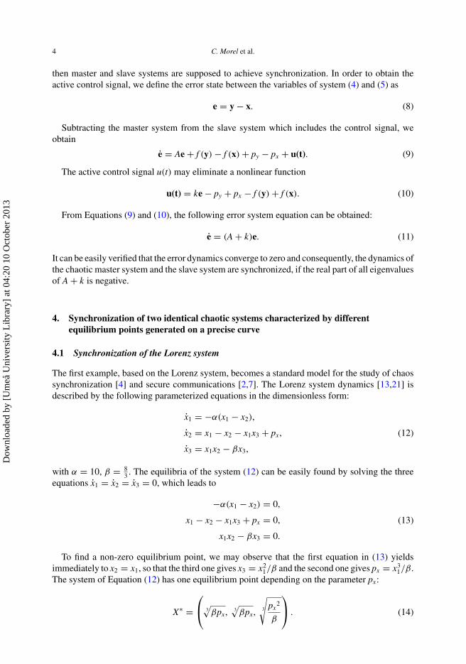
original system Lorenz, Jerk or Van der Pol, is based on a switching piecewise-constant controllerto generated several independent chaotic attractors in a controllable state space area, a curve.Before the chaos synchronization, the two identical chaotic systems are characterized by thesame or by two different stable equilibrium points. Then, by addition of a coupling term, chaossynchronization forces the slave system to leave its own basin of attraction and to trace the mastersystem: the states of two identical systems are globally synchronized.
We introduce a modified Lorenz system to ensure that this method can also be used for twochaotic systems with different structures and with equilibrium points distributed anywhere inthe state space. This original system developed in [16] generates several independent chaoticattractors in a controllable state space area of a paraboloid. In this case, the two chaotic systemsare characterized by two different stable equilibrium points on different parabola either of the sameparaboloid or of different paraboloids. The main goal of this paper is to force the slave system toleave its basin of attraction and to trace the master system, by addition of a coupling term. Thestate variables of the two systems become ultimately the same using the active control technique.
2. Generating independent chaotic attractors in a nonlinear system
Consider a three-dimensional nonlinear autonomous system:
x = fpx (x), x(0) = x0, t ∈ R+, (1)
where x = (x1, x2, x3)T ∈ R
3, px ∈ P ⊆ R is a real parameter and fpx : R3 → R
3 a nonlinear vectorfunction.
The equilibria of the system (1) are found by solving the equations fpx (x) = 0. The graphical rep-resentation of these equilibria in function of the parameter px gives a precise curve in the state spaceR
3. Let us take into account a variation of px ∈ P as follows, for which the equilibria are stable:
a ≤ px ≤ b. (2)
We introduce the following notations: X is the set of all equilibrium points, � is the set of allcorresponding curves and �X∗ is the curve corresponding to the equilibrium point X∗ ∈ X .
Considering the Jacobian matrix for the equilibria and calculating its characteristic equation,we can investigate the stability of each equilibrium based on the Routh–Hurwitz conditions ofthe system characteristic equation. We determine the parameter variation domain such as theequilibria are stable.
Suppose that X∗ is stable for px ∈ [a, b] and the projections of �X∗ are the single intervals[x1a; x1b], [x2a; x2b], [x3a; x3b] (Figure 1).
In this paper, we are interested in generating several independent chaotic attractors on the 3Ddomain on some curve �X∗ , by switching the control parameter px (between the values a and b).
Recently, in [19] a periodic nonlinearity of px such as μ sin(x(t − τ))[1 + ε sin(x2(t − τ))]has been considered. The global behaviour of the delay model shows the co-existence of trivialattractors (fixed point or limit cycle) and chaotic attractors (with stable and unstable equilibria)generated in a precise state space for ε < 1 and μτ < π/2. With another nonlinear function px,ε sin(σx(t − τ)), Wang et al. [21] obtained only two separated chaotic attractors near two stablefixed points for large values of σ . In order to generate independent chaotic attractors [10] for thesystem (1) on the bold curve of Figure 1, a piecewise-constant characteristic [3,9] of the feedbackcontroller px, is defined analytically as follows:
px ={
b, sin(δt) < ε sin(σx1(t)),
a, sin(δt) ≥ ε sin(σx1(t)).(3)
Dow
nloa
ded
by [
Um
eå U
nive
rsity
Lib
rary
] at
04:
20 1
0 O
ctob
er 2
013

International Journal of Computer Mathematics 3
a
aa
Figure 1. Example of system (1) equilibria on three-dimensional state space.
as in [14,21]. The fast switching of the controller of Equation (3) between the levels a and bdetermines small variations of the state variables and an attraction of the state variable x1 first tox1a and then to x1b, and so on.
The dynamical state space trajectory remains around the equilibrium point, inside its ownbasin of attraction without switching to the basin of attraction of the neighbouring attractors, foreach attractor starting from different initial conditions. With the anticontrol switching piecewise-constant controller of Equation (3), the attractors will be chaotic along �X∗ for px ∈ [a, b] (seethe thick line in Figure 1). The study of the chaotic attractors shows an equidistant repartition inthe state space. We have introduced in [14] and further developed in [15,16] that the attractorsperiodicity in the state space depends on the sine anticontrol feedback frequency given by: dx1 =2π/σ , the distance on the x1 axis between two consecutive transitions b → a of px.
3. Problem formulation and synchronization analysis
Consider the chaotic master system, described by the dynamics
x = Ax + f (x) + px, (4)
where x = (x1, x2, . . . , xN )T ∈ RN is the state vector, A ∈ R
N×N is a constant matrix, f (x) is anonlinear function and px is the piecewise-constant controller described by the Equation (3).
The slave system is
y = Ay + f (y) + py + u(t), (5)
where y = (y1, y2, . . . , yN )T ∈ RN , u(t) is the active control signal that is yet to be determined.
For the slave system, py is the piecewise-constant controller defined as follows:
py ={
b, sin(δt) < ε sin(σy1(t)),
a, sin(δt) ≥ ε sin(σy1(t)).(6)
The aim of the active control signal is to force the slave system to follow the master system. Ifthere exists an appropriate control signal u(t) satisfying
limt→∞ e(t) = lim
t→∞(y(t) − x(t)) = 0, (7)
Dow
nloa
ded
by [
Um
eå U
nive
rsity
Lib
rary
] at
04:
20 1
0 O
ctob
er 2
013
4 C. Morel et al.
then master and slave systems are supposed to achieve synchronization. In order to obtain theactive control signal, we define the error state between the variables of system (4) and (5) as
e = y − x. (8)
Subtracting the master system from the slave system which includes the control signal, weobtain
e = Ae + f (y) − f (x) + py − px + u(t). (9)
The active control signal u(t) may eliminate a nonlinear function
u(t) = ke − py + px − f (y) + f (x). (10)
From Equations (9) and (10), the following error system equation can be obtained:
e = (A + k)e. (11)
It can be easily verified that the error dynamics converge to zero and consequently, the dynamics ofthe chaotic master system and the slave system are synchronized, if the real part of all eigenvaluesof A + k is negative.
4. Synchronization of two identical chaotic systems characterized by differentequilibrium points generated on a precise curve
4.1 Synchronization of the Lorenz system
The first example, based on the Lorenz system, becomes a standard model for the study of chaossynchronization [4] and secure communications [2,7]. The Lorenz system dynamics [13,21] isdescribed by the following parameterized equations in the dimensionless form:
x1 = −α(x1 − x2),
x2 = x1 − x2 − x1x3 + px,
x3 = x1x2 − βx3,
(12)
with α = 10, β = 83 . The equilibria of the system (12) can be easily found by solving the three
equations x1 = x2 = x3 = 0, which leads to
−α(x1 − x2) = 0,
x1 − x2 − x1x3 + px = 0,
x1x2 − βx3 = 0.
(13)
To find a non-zero equilibrium point, we may observe that the first equation in (13) yieldsimmediately to x2 = x1, so that the third one gives x3 = x2
1/β and the second one gives px = x31/β.
The system of Equation (12) has one equilibrium point depending on the parameter px:
X∗ =⎛⎝ 3
√βpx, 3
√βpx, 3
√px
2
β
⎞⎠ . (14)
Dow
nloa
ded
by [
Um
eå U
nive
rsity
Lib
rary
] at
04:
20 1
0 O
ctob
er 2
013

International Journal of Computer Mathematics 5
Figure 2. The independent chaotic attractors of the Lorenz system (12) (colour online only).
Table 1. State space equilibria intervals for different values of thepiecewise-constant controller of the Lorenz system.
Group of attractors a b x1, x2 of Equation (15) x3 of Equation (16)
I 0 0.5 [0, 1.1] [0, 0.45]II 1 2 [1.3867, 1.747] [0.721, 1.145]III −1.5 −0.5 [−1.587, −1.1] [0.454, 0.945]
A static variation of px between a and b imposes the intervals to the equilibrium X∗ on the x1,x2 and x3 state space as follows:
on the x1 and x2 axes: [ 3√
aβ, 3√
bβ], (15)
on the x3 axis:
⎡⎣ 3
√a2
β, 3
√b2
β
⎤⎦ . (16)
We consider now a fast dynamics variation of px given by the anticontrol switching piecewise-constant controller px of Equation (3), with γ = 1000, σ = 100 and ε = 5. The independentchaotic attractors of the Lorenz system (12) are generated inside the state space of Equations (15)and (16) from different initial conditions. The attractors are situated in the plane x1 = x2, and onthe parabola x3 = 3x2
1/8 represented in Figure 2 with the fine curve. Table 1 presents the equilibriaintervals on each axis x1, x2 and x3 for three different values of a and b. Figure 2 shows where thegenerated attractors groups are situated inside a precise state space given by Table 1.
In order to synchronize two Lorenz systems (with the same or different regimes of operationof the same attractors group), we consider the master system (12) and the slave system defined asfollows:
y1 = −α(y1 − y2),
y2 = y1 − y2 − y1y3 + py + u,
y3 = y1y2 − βy3.
(17)
Dow
nloa
ded
by [
Um
eå U
nive
rsity
Lib
rary
] at
04:
20 1
0 O
ctob
er 2
013
6 C. Morel et al.
Starting from the same initial conditions and using the slave system, the same group of attractorscan be obtained if the active signal is u(t) = 0.
Subtracting Equation (12) from Equation (17) gives
e1 = α(e2 − e1),
e2 = e1 − e2 − y1y3 + x1x3 + py − px + u,
e3 = y1y2 − x1x2 − βe3,
(18)
where e1 = y1 − x1, e2 = y2 − x2 and e3 = y3 − x3 are the errors. In order to determine thefeedback control signal u(t), the Lyapunov function V is
V(e) = 12 (e2
1 + e22 + e2
3); (19)
it has the time derivative:
V = e1e1 + e2e2 + e3e3 = −αe21 − e2
2 − βe23 + x2e1e3
+ (α + 1)e1e2 − e1e2x3 + e2(py − px + u). (20)
A trivial choice of u is
u(t) = −py + px − (α + 1)e1 + e1x3 + ke2. (21)
In this case Equation (20) becomes
V = (k − 1)e22 − αe2
1 + e1x2e3 − βe23. (22)
The derivative Lyapunov function (22) is V < 0 if k < 1 and x2 <√
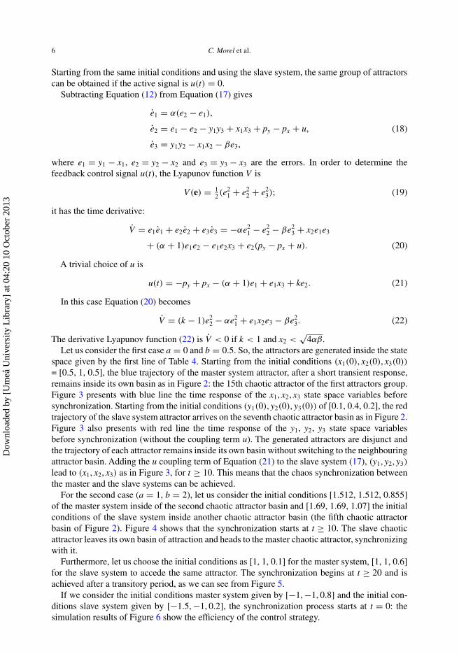
4αβ.Let us consider the first case a = 0 and b = 0.5. So, the attractors are generated inside the state
space given by the first line of Table 4. Starting from the initial conditions (x1(0), x2(0), x3(0))
= [0.5, 1, 0.5], the blue trajectory of the master system attractor, after a short transient response,remains inside its own basin as in Figure 2: the 15th chaotic attractor of the first attractors group.Figure 3 presents with blue line the time response of the x1, x2, x3 state space variables beforesynchronization. Starting from the initial conditions (y1(0), y2(0), y3(0)) of [0.1, 0.4, 0.2], the redtrajectory of the slave system attractor arrives on the seventh chaotic attractor basin as in Figure 2.Figure 3 also presents with red line the time response of the y1, y2, y3 state space variablesbefore synchronization (without the coupling term u). The generated attractors are disjunct andthe trajectory of each attractor remains inside its own basin without switching to the neighbouringattractor basin. Adding the u coupling term of Equation (21) to the slave system (17), (y1, y2, y3)
lead to (x1, x2, x3) as in Figure 3, for t ≥ 10. This means that the chaos synchronization betweenthe master and the slave systems can be achieved.
For the second case (a = 1, b = 2), let us consider the initial conditions [1.512, 1.512, 0.855]of the master system inside of the second chaotic attractor basin and [1.69, 1.69, 1.07] the initialconditions of the slave system inside another chaotic attractor basin (the fifth chaotic attractorbasin of Figure 2). Figure 4 shows that the synchronization starts at t ≥ 10. The slave chaoticattractor leaves its own basin of attraction and heads to the master chaotic attractor, synchronizingwith it.
Furthermore, let us choose the initial conditions as [1, 1, 0.1] for the master system, [1, 1, 0.6]for the slave system to accede the same attractor. The synchronization begins at t ≥ 20 and isachieved after a transitory period, as we can see from Figure 5.
If we consider the initial conditions master system given by [−1, −1, 0.8] and the initial con-ditions slave system given by [−1.5, −1, 0.2], the synchronization process starts at t = 0: thesimulation results of Figure 6 show the efficiency of the control strategy.
Dow
nloa
ded
by [
Um
eå U
nive
rsity
Lib
rary
] at
04:
20 1
0 O
ctob
er 2
013

International Journal of Computer Mathematics 7
0 5 10 15 200
0.2
0.4
0.6
0.8
1
Time t(s)
Stat
e va
riab
les
x 1 and
y1
(a)
0 5 10 15 200.2
0.4
0.6
0.8
1
1.2
Time t(s)
Stat
e va
riab
les
x 2 and
y2
(b)
0 5 10 15 200
0.1
0.2
0.3
0.4
0.5
Time t(s)
Stat
e va
riab
les
x 3 and
y3
(c)
Figure 3. x1(t), x2(t) and x3(t) of the master system (12) starting from the initial conditions(x1(0), x2(0), x3(0)) = [0.5, 1, 0.5] and y1(t), y2(t) and y3(t) of the slave system (17) starting from the initialconditions (y1(0), y2(0), y3(0)) = [0.1, 0.4, 0.2] (colour online only).
0 5 10 15 201.4
1.5
1.6
1.7
1.8
1.9
Time t(s)
Stat
e va
riab
les
x 1 and
y1
(a)
0 5 10 15 201.4
1.5
1.6
1.7
1.8
1.9
Time t(s)
Stat
e va
riab
les
x 2 and
y2
(b)
0 5 10 15 200.85
0.9
0.95
1
1.05
1.1
Time t(s)St
ate
vari
able
s x 3 a
nd y
3
(c)
Figure 4. x1(t), x2(t) and x3(t) of the master system (12) starting from the initial conditions(x1(0), x2(0), x3(0)) = [1.512, 1.512, 0.855] and y1(t), y2(t) and y3(t) of the slave system (17) starting from theinitial conditions (y1(0), y2(0), y3(0)) = [1.69, 1.69, 1.07].
(a) (b) (c)
19 20 21 22 23
1.625
1.63
1.635
1.64
1.645
Time t(s)
Stat
e va
riab
les
x 1 and
y1
19 19.5 20 20.5 21 21.5
1.6
1.61
1.62
1.63
1.64
1.65
1.66
1.67
Time t(s)
Stat
e va
riab
les
x 2 and
y2
18 19 20 21 22 23
0.99
0.995
1
1.005
1.01
Time t(s)
Stat
e va
riab
les
x 3 and
y3
Figure 5. x1(t), x2(t) and x3(t) of the master system (12) starting from the initial conditions(x1(0), x2(0), x3(0)) = [1, 1, 0.1] and y1(t), y2(t) and y3(t) of the slave system (17) starting from the initialconditions (y1(0), y2(0), y3(0)) = [1, 1, 0.6].
(a) (b) (c)
0 2 4 6 8 10−1.5
−1.4
−1.3
−1.2
−1.1
−1
−0.9
−0.8
Time t(s)
Stat
e va
riab
les
x 1 and
y1
0 2 4 6 8 10−1.4
−1.3
−1.2
−1.1
−1
−0.9
−0.8
−0.7
Time t(s)
Stat
e va
riab
les
x 2 and
y2
0 2 4 6 8 100.2
0.3
0.4
0.5
0.6
0.7
0.8
0.9
1
Time t(s)
Stat
e va
riab
les
x 3 and
y3
Figure 6. x1(t), x2(t) and x3(t) of the master system (12) starting from the initial conditions(x1(0), x2(0), x3(0)) = [−1, −1, 0.8] and y1(t), y2(t) and y3(t) of the slave system (17) starting from the initialconditions (y1(0), y2(0), y3(0)) = [−1.5, −1, 0.2].
Dow
nloa
ded
by [
Um
eå U
nive
rsity
Lib
rary
] at
04:
20 1
0 O
ctob
er 2
013

8 C. Morel et al.
Figure 7. Independent chaotic attractors of the Jerk system of Equation (23).
4.2 Synchronization of the Jerk system
Let us take an other example, the Jerk system [25], described by...x + Mx + x = g(x), where M
is a real parameter and g(x) a nonlinear function g(x) = 1 − |x| as in [8,20]. The inclusion of theanticontrol switching piecewise-constant controller px in the Jerk system is determined by
x1 = x2 + px,
x2 = x3,
x3 = −Mx3 − x2 − |x1| + 1.
(23)
Using px as the control parameter, the equilibria of the system (23) leads to: x2 = −px, x3 = 0,and |x1| = 1 − x2. We obtain X∗+ and X∗−, symmetrically placed with respect to the x1-axis:
X∗+ = (px + 1, −px, 0),
and
X∗− = (−px − 1, −px, 0). (24)
The stability of this equilibrium based on the Routh–Hurwitz conditions on the Jerk system (23)characteristic equation can be investigated. Therefore,
P(λ) = λ3 + Mλ2 + λ + 1. (25)
A necessary and sufficient condition for the stability of the equilibrium points X∗+ and X∗− is givenby the condition M − 1 > 0.
Dow
nloa
ded
by [
Um
eå U
nive
rsity
Lib
rary
] at
04:
20 1
0 O
ctob
er 2
013

International Journal of Computer Mathematics 9
Table 2. State space equilibria intervals and different values of the piecewise-constant controller of Jerk system imposingthe x1 state space domain.
Group of attractors c d of Equation (27) x2 of Equations (28) and (35) px
I −3 −2.25 [−2, −1.25] [1.25, 2]II 1.25 2 [−1, −0.25] [0.25, 1]III −0.8 0 [0.2, 1] [−1, −0.2]
This time, we want to have chaotic attractors on the state space between the limits c and d foran x1 axis projection:
on the x1 axis: [c; d]. (26)
The state space domain for an x2 axis projection is
on the x2 axis:
{[1 − d, 1 − c] if c ≥ 0,
[1 + c, 1 + d] if c < 0.(27)
Substituting Equation (27) into x2 = −px, the anticontrol switching piecewise-constant controllerpx has the form:
if c ≥ 0, px ={
c − 1, sin(δt) ≥ ε sin(σx1(t)),
d − 1, sin(δt) < ε sin(σx1(t)),(28)
and
if c < 0, px ={
−1 − d, sin(δt) ≥ ε sin(σx1(t)),
−1 − c, sin(δt) < ε sin(σx1(t)).(29)
For M = 2.017 as in [20], the equilibrium points X∗+ and X∗− are stable.The limits imposed to the state space domain for an x1 axis projection (c and d), the state space
domain for an x2 axis projection calculated with Equation (27), the switch levels of the anticontrolswitching piecewise-constant controller px of Equations (28) and (29) are presented in Table 2.
For three values of the anticontrol switching piecewise-constant controller px (fifth column ofTable 2), Figure 8 presents three groups of independent chaotic attractors.
Let us synchronize two Jerk systems which generate attractors in the same group. We considerthe master system (23) and the slave system chosen as
y1 = y2 + py + u,
y2 = y3,
y3 = −My3 − y2 − |y1| + 1.
(30)
The system (30) is a slave of system (23) if the error system
e1 = e2 + py − px + u,
e2 = e3,
e3 = −Me3 − e2 − |y1| + |x1|(31)
is asymptotically stable at the origin. If we choose a Lyapunov function of the form Equation (19),its derivative along the solution of Equation (31) is
V = e1e2 + e1(py − px) + ue1
− Me23 + e3(|x1| − |y1|). (32)
Dow
nloa
ded
by [
Um
eå U
nive
rsity
Lib
rary
] at
04:
20 1
0 O
ctob
er 2
013

10 C. Morel et al.
If we choose
u(t) = ke1 − e2 + px − py − (|x1| − |y1|)e3
e1, (33)
Equation (32) can then be rewritten as
V = −Me23 + ke2
1. (34)
This means that chaos synchronization between Jerk systems can be achieved if k < 0.For the first or the third groups of independent chaotic attractors, x1, y1 < 0, then |x1| − |y1| =
−x1 + y1 = e1. For the second group of independent chaotic attractors, x1, y1 >0, then |x1| −|y1| = x1 − y1 = −e1. In this case Equation (33) can be written
u(t) ={
ke1 − e2 + px − py − e3, x1, y1 < 0,
ke1 − e2 + px − py + e3, x1, y1 > 0.(35)
The slave system is
y1 = y2 + px + ke1 − e2 − e3,
y2 = y3,
y3 = −My3 − y2 − |y1| + 1,
(36)
or
y1 = y2 + px + ke1 − e2 + e3,
y2 = y3,
y3 = −My3 − y2 − |y1| + 1,
(37)
in function of the attractors group. In these cases, the error dynamics can be written as follows:
e1 = ke1 − e3,
e2 = e3,
e3 = e1 − e2 − Me3,
(38)
or
e1 = ke1 + e3,
e2 = e3,
e3 = −e1 − e2 − Me3.
(39)
Equations (38) and (39) can be rewritten as
e =⎡⎣k 0 −1
0 0 11 −1 −M
⎤⎦ e, (40)
or
e =⎡⎣ k 0 +1
0 0 1−1 −1 −M
⎤⎦ e, (41)
which provide the same characteristic equation:
λ3 + (M − k)λ2 + (2 − Mk)λ − k = 0. (42)
If each eigenvalue is negative, e converges to zero. Designing k = −2, leads to negative real parteigenvalues: −0.45, −1.782 and −1.782.
Dow
nloa
ded
by [
Um
eå U
nive
rsity
Lib
rary
] at
04:
20 1
0 O
ctob
er 2
013

International Journal of Computer Mathematics 11
0 10 20 30 40 50 60−0.4
−0.2
0
0.2
0.4
0.6
0.8
1
Time t(s)
Err
ors
e 1(t),
e2(t
) an
d e 3(t
)(a)
0 10 20 30 40 50 60−0.4
−0.3
−0.2
−0.1
0
0.1
0.2
0.3
0.4
Time t(s)
Err
ors
e 1(t),
e2(t
) an
d e 3(t
)
(b)
0 10 20 30 40 50 60−0.4
−0.3
−0.2
−0.1
0
0.1
0.2
0.3
Time t(s)
Err
ors
e 1(t),
e2(t
) an
d e 3(t
)
(c)
Figure 8. (a) Time history of errors e1(t), e2(t) and e3(t) with the initial conditions (x1(0), x2(0), x3(0)) =[−2.8 − 1.3 0], of the Jerk system (23) and with the initial conditions (y1(0), y2(0), y3(0)) = [−2 − 0.5 0], of theJerk system (30) with the activation of the feedback control after t ≥ 0; (b) Time history of errors e1(t), e2(t) and e3(t)with the initial conditions (x1(0), x2(0), x3(0)) = [−2.8 − 1.3 0], of the Jerk system (23) and with the initial conditions(y1(0), y2(0), y3(0)) = [−2 − 0.5 0], of the Jerk system (30) with the activation of the feedback control after t ≥ 0; (c)time history of errors e1(t), e2(t) and e3(t) with the initial conditions (x1(0), x2(0), x3(0)) = [−0.5 0.7 0], of the Jerksystem (23) and with the initial conditions (y1(0), y2(0), y3(0)) = [−0.7 1 0], of the Jerk system (30) with the activationof the feedback control after t ≥ 20.
For the first group of attractors of Table 2, the chaos synchronization starts at t = 0. Thenumerical results of the uni-directional coupling method are shown in Figure 8. Let us choose theinitial conditions as [1.912 − 0.9130] for the master system, [1.54 − 0.540] for the slave systemof the second group of attractors. The synchronization begins at t ≥ 20 and is achieved after atransitory period, as can be seen from Figure 8. The same phenomena can be observed in Figure 8for the third group of attractors. Then the synchronism process begins, the attractor of the slavesystem is taken out of its own basin of attraction and is attracted towards the master chaoticattractor.
4.3 Synchronization of the Van der Pol system
In this section, independent chaotic attractors are generated from the Van der Pol system [6,11],which can be written by the following equations:
x1 = x2,
x2 = −x1 − 3 · (x21 − 1)x2 + px.
(43)
The equilibria of the system (43) lead to the following relations:
x2 = 0, x1 = px. (44)
The Van der Pol system of Equation (43) has one equilibrium point:
X∗ = (px, 0). (45)
As discussed previously, Equations (44) enable the calculation of equilibria intervals for avariation of px between the limits a and b:
on the x1 axis: [a, b]. (46)
The independent chaotic attractors are generated inside the state space of Equation (46) aroundx2 = 0. Table 3 contains the state domain x1 for three different anticontrol switching piecewiseconstant controllers px.
Dow
nloa
ded
by [
Um
eå U
nive
rsity
Lib
rary
] at
04:
20 1
0 O
ctob
er 2
013

12 C. Morel et al.
Table 3. State space equilibria intervals and different values of thepiecewise-constant controller of the Van der Pol system.
Group ofattractors a b x1 of Equation (46)
I −3 −2 [−3, −2]II 1 2 [1, 2]III 3.5 4.5 [3.5, 4.5]
Figure 9. Independent chaotic attractors of the Van der Pol system of Equation (43).
TheVan der Pol system simulations present independent chaotic attractors, as shown in Figure 9.The attractors, generated from different initial conditions, are situated on the line x2 = 0 repre-sented in Figure 9 with the fine curve. For the three intervals of px, the projections of the attractorsonto x1 − x2 plane show that all attractors are situated inside the state space given by Table 3.
Let us synchronize the master Van der Pol system (43) with the slave Van der Pol system of thefollowing form:
y1 = y2,
y2 = −y1 − 3 · (y21 − 1)y2 + py + u.
(47)
The Van der Pol system error is
e1 = e2,
e2 = −e1 − 3 · (y21 − 1)y2 + 3 · (x2
1 − 1)x2 + py − px + u.(48)
As in the previous examples, the derivative Lyapunov function can be written as
V = e2(py − px + u) + 3e2(x21x2 − y2
1y2 − e2). (49)
We find a controller u defined by
u(t) = px − py + ke2 − 3e2 − 3(x21x2 − y2
1y2), (50)
Dow
nloa
ded
by [
Um
eå U
nive
rsity
Lib
rary
] at
04:
20 1
0 O
ctob
er 2
013

International Journal of Computer Mathematics 13
Figure 10. x1(t) (blue line) with the initial conditions x1(0) = −2.2, x2(0) = −0.25 of the Van der Pol system (43) andy1(t) (red line) with the initial conditions y1(0) = −2.8, y2(0) = 0.2 of the Van der Pol system (47) (colour online only).Phase plot of the synchronization between x1 and y1 and between x2 and y2 (the first 1000 points were omitted).
Figure 11. x1(t) (blue line) with the initial conditions x1(0) = 1.2, x2(0) = −0.25 of the Van der Pol system (43) andy1(t) (red line) with the initial conditions y1(0) = 1.8, y2(0) = 0.2 of the Van der Pol system (47) (colour online only).Phase plot of the synchronization between x1 and y1 and between x2 and y2 (the first 1000 points were omitted).
Figure 12. x1(t) (blue line) with the initial conditions x1(0) = 3.6764, x2(0) = 0 of the Van der Pol system (43) andy1(t) (red line) with the initial conditions y1(0) = 4.4288, y2(0) = 0 of the Van der Pol system (47) (colour online only).Phase plot of the synchronization between x1 and y1 and between x2 and y2 (the first 1000 points were omitted).
such that
V = ke22 (51)
is clearly a negative definite function if k < 0. Then, the error dynamics (48) simplifies to
e =[
0 1−1 k
]e. (52)
This equation leads to negative eigenvalues 12 (k ± √
k2 − 4). The two systems (43) and (47) areglobally asymptotically synchronized under the controller (50), if k is chosen to satisfy k < 0.
The results of the two identical chaotic systems with active control are shown: in Figure 10 forthe first group of attractors, in Figure 11 for the second group of attractors and in Figure 12 forthe third group of attractors described in Table 3.
Let us take different initial values of the two Van der Pol systems for the first attractor group:the initial values of the master Van der Pol system (43) are x1(0) = −2.2, x2(0) = −0.25 and
Dow
nloa
ded
by [
Um
eå U
nive
rsity
Lib
rary
] at
04:
20 1
0 O
ctob
er 2
013

14 C. Morel et al.
the initial values of the slave Van der Pol system (47) are y1(0) = −2.8, y2(0) = 0.2. Figure 10shows the phase portrait of unsynchronized case: the master Van der Pol system (43) joints thethirteenth attractor with blue line and slave Van der Pol system (47) attracts the fourth attractorin red. After synchronization, the slave system is extracted from its stable position and joins thethirteenth attractor of the master Van der Pol system. The synchronizations of the state x1 versus y1
and of the state x2 versus y2 are shown in Figure 10. Simulation results show that the two systemssynchronize well. Starting from different initial values x1(0) = 1.2, x2(0) = −0.25 of the Van derPol system (43) and y1(0) = 1.8, y2(0) = 0.2 of the Van der Pol system (47), the synchronizationprocess starts at the beginning for the second group of attractors. Omitting the first 1000 points ofthe phase plot responses, Figure 11 shows a good synchronization between x1 and y1 and betweenx2 and y2, respectively.
For the third group of attractors, some simulation results are plotted in Figure 12 and verify thevalidity of the synchronization reached by one way coupling, even if the initial systems belong totwo different basins of attraction.
5. Synchronization of two different chaotic systems characterized by differentequilibrium points distributed anywhere in the state space on the paraboloid
In order to illustrate the proposed approach, we consider a system dynamics described by thefollowing parameterized equations:
x1 = α(x2 cos θx − x1 sin θx),
x2 = x1 sin θx − x2 cos θx − x1x3 + px,
x3 = x21 + x2
2 − βxx3,
(53)
which are in the form (1). To find a non-trivial equilibrium point, we may observe that the firstequation in (53) yields to
x2 = x1sin θx
cos θx. (54)
So that the third one gives
x3 = x21 + x2
2
βx= x2
1
βx cos2 θx(55)
and the second one gives
px = x1x3 = x31
βx cos2 θx. (56)
The system (53) has one equilibrium point depending on px. Thus:
X∗ =⎛⎝ 3
√pxβx cos2 θx, sin θx
3
√pxβx
cos θx, 3
√px
2
βx cos2 θx
⎞⎠ . (57)
Dow
nloa
ded
by [
Um
eå U
nive
rsity
Lib
rary
] at
04:
20 1
0 O
ctob
er 2
013
International Journal of Computer Mathematics 15
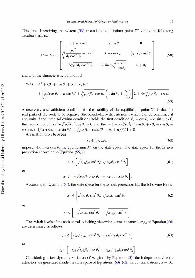
This time, linearizing the system (53) around the equilibrium point X∗ yields the followingJacobian matrix:
λI − JX∗ =
⎡⎢⎢⎢⎢⎢⎢⎣
λ + α sin θx −α cos θx 0
3
√px
2
βx cos2 θx− sin θx λ + cos θx
3√
pxβx cos2 θx
−2 3√
pxβx cos2 θx −2 sin θx3
√pxβx
cos θxλ + βx
⎤⎥⎥⎥⎥⎥⎥⎦
(58)
and with the characteristic polynomial
P(λ) = λ3 + (βx + cos θx + α sin θx)λ2
+[βx(cos θx + α sin θx) + 3
√px
2βx2 cos θx
(2 sin θx + α
βx
)]λ + 3α
3
√px
2βx2 cos θx.
(59)
A necessary and sufficient condition for the stability of the equilibrium point X∗ is that thereal parts of the roots λ be negative (the Routh–Hurwitz criterion), which can be confirmed ifand only if the three following conditions hold: the first condition βx + cos θx + α sin θx > 0,the second condition 3α
3√
px2βx
2 cos θx > 0 and the last −3α3√
px2βx
2 cos θx + (βx + cos θx +α sin θx) · [βx(cos θx + α sin θx) + 3
√px
2βx2 cos θx(2 sin θx + α/βx)] > 0.
A variation of x3 between
x3 ∈ [x3a; x3b] (60)
imposes the intervals to the equilibrium X∗ on the state space. The state space for the x1 axisprojection according to Equation (55) is
x1 ∈[√
x3aβx cos2 θx;√
x3bβx cos2 θx
](61)
or
x1 ∈[−
√x3bβx cos2 θx; −
√x3aβx cos2 θx
].
According to Equation (54), the state space for the x2 axis projection has the following form:
x2 ∈[√
x3aβx sin2 θx;√
x3bβx sin2 θx
](62)
or
x2 ∈[−
√x3bβx sin2 θx; −
√x3aβx sin2 θx
].
The switch levels of the anticontrol switching piecewise-constant controller px of Equation (56)are determined as follows:
px ∈[x3a
√x3aβx cos2 θx; x3b
√x3bβx cos2 θx
](63)
or
px ∈[−x3b
√x3bβx cos2 θx; −x3a
√x3aβx cos2 θx
].
Considering a fast dynamic variation of px given by Equation (3), the independent chaoticattractors are generated inside the state space of Equations (60)–(62). In our simulations, α = 10,
Dow
nloa
ded
by [
Um
eå U
nive
rsity
Lib
rary
] at
04:
20 1
0 O
ctob
er 2
013

16 C. Morel et al.
Table 4. The system (53): α = 10, σ = 100 and ε = 5.
x1 x2 pxParaboloid Curve βx θx x3a x3b Equation (61) Equation (62) Equation (63)
Paraboloid I Parabola 1 83 π/6 0.1 0.6 [0.45, 1.09] [0.26, 0.63] [0.04, 0.66]
Parabola 2 5π/12 0 0.7 [0, 0.35] [0, 1.32] [0, 0.247]Parabola 3 4π/3 0.1 0.75 [−0.71, −0.26] [−1.22, −0.45] [−0.53, −0.026]
Paraboloid II Parabola 4 203 π/3 0.1 0.5 [0.4, 0.91] [0.707, 1.58] [0.04, 0.45]
Parabola 5 7π/6 0.2 0.5 [−1.58, −1] [−0.91, −0.57] [−0.79, −0.2]Parabola 6 17π/12 0 0.5 [−0.47, 0] [−1.76, 0] [−0.434, 0]
Figure 13. First paraboloid: the independent chaotic attractors generation of the system (53) on the curves 1, 2and 3. Second paraboloid: the independent chaotic attractors generation of the system (53) on the curves 4, 5and 6.
σ = 100 and ε = 5. Therefore the equilibrium point X∗ of (57) is stable. We list in Table 4 theequilibria intervals on each axis x1, x2 and x3 (derived from Equations (60)–(62)) for six differentvalues of x3a and x3b.
Figure 13 shows the independent chaotic attractors of the system (53). The attractors, gen-erated from different initial conditions, are situated in the plane x2 = x1(sin θx/ cos θx), and onthe parabola x3 = (x2
1 + x22)/βx represented in Figure 13 with the fine curve. The independent
attractors are generated on this fine curve on a precise zone according to the x3a and x3b valuesof x3 (as for curve 1). With a variation of θx, the attractors are situated on other parabola (curve2 or curve 3). In the 3D state space, the curves are situated on the first paraboloid and the attrac-tors too. Generating attractors to a different paraboloid and different curves is possible accordingto βx.
In order to synchronize two systems with the same or different regime of operation of thesame or different attractors group of the same or different paraboloid, we consider the master
Dow
nloa
ded
by [
Um
eå U
nive
rsity
Lib
rary
] at
04:
20 1
0 O
ctob
er 2
013
International Journal of Computer Mathematics 17
system (53) and the slave system designed as follows:
y1 = α(y2 cos θy − y1 sin θy) + u1,
y2 = y1 sin θy − y2 cos θy − y1y3 + py + u2,
y3 = y21 + y2
2 − βyy3 + u3.
(64)
Starting from the same initial conditions and using the slave system, the same groups of attrac-tors can be obtained if the active signals are u1(t) = 0, u2(t) = 0 and u3(t) = 0. SubtractingEquation (53) from Equation (64) gives
e1 = α(y2 cos θy − y1 sin θy − x2 cos θx + x1 sin θx) + u1,
e2 = y1 sin θy − y2 cos θy − y1y3 + py − x1 sin θx + x2 cos θx + x1x3 − px + u2,
e3 = y21 + y2
2 − βyy3 − x21 − x2
2 + βxx3 + u3,
(65)
where e1 = y1 − x1, e2 = y2 − x2 and e3 = y3 − x3 are the errors. In order to determine thefeedback control signals u1, u2 and u3, the Lyapunov function V is:
V(e) = 12 (e2
1 + e22 + e2
3); (66)
it has the time derivative:
V = e1e1 + e2e2 + e3e3
= e1α(y2 cos θy − y1 sin θy − x2 cos θx + x1 sin θx) + e1u1
+ e2(y1 sin θy − y2 cos θy − y1y3 + py − x1 sin θx + x2 cos θx + x1x3 − px + u2)
+ e3(y21 + y2
2 − βyy3 − x21 − x2
2 + βxx3 + u3). (67)
A trivial choice of u1, u2 and u3 is
u1 = −k1e1 + α(x2 cos θx − x1 sin θx − y2 cos θy + y1 sin θy),
u2 = −k2e2 + px − py + y1y3 − x1x3 − y1 sin θy + y2 cos θy − x2 cos θx + x1 sin θx,
u3 = −k3e3 − e1(x1 + y1) − e2(x2 + y2) + βyy3 − βxx3.
(68)
In this case, Equation (67) becomes
V = −k1e21 − k2e2
2 − k3e32. (69)
The derivative Lyapunov function (69) is V < 0 if k1 > 0, k2 > 0 and k3 > 0.
5.1 Case 1: synchronization of the chaotic attractors which below to the same paraboloid I
Let us consider the first case when the attractors to be synchronized belong to the same paraboloidI (as in Figure 14) and much more to the same parabola 1. In this case, βx = βy = 8
3 and θx =θy = π/6, as in the first line of Table 5.
Starting from the initial conditions (x1(0), x2(0), x3(0)) = [0.1, −0.3, 0.3], the blue trajectoryof the master system attractor, after a short transient response, remains inside its own basin as inFigure 14: the fifth chaotic attractor of the attractors group of parabola 1. Figure 15 presents withblue line the time response of the x1, x2, x3 state space variables before synchronization.
Starting from the initial conditions (y1(0), y2(0), y3(0)) of [1, 1, 0.7], the red trajectory of theslave system attractor arrives on the seventh chaotic attractor basin as in Figure 14. Figure 15 also
Dow
nloa
ded
by [
Um
eå U
nive
rsity
Lib
rary
] at
04:
20 1
0 O
ctob
er 2
013

18 C. Morel et al.
Table 5. Different cases of synchronization: α = 10.
Case 1: Master SlaveFigure 14 Paraboloid I Paraboloid I βx βy θx θy x(0) of Master y(0) of Slave
Figure 15 Parabola 1 Parabola 1 83
83 π/6 π/6 [0.1; −0.3; 0.3] [1; 1; 0.7]
Figure 16 Parabola 3 Parabola 2 83
83 4π/3 5π/12 [0.8; −0.8; 0.3] [1; 1; 0.1]
Figure 17 Parabola 2 Parabola 3 83
83 5π/12 4π/3 [0.2; 1; 0.1] [−1; −1; 0.3]
Figure 14. Synchronization of the chaotic attractors which belong to the same paraboloid I (colour online only).
0 5 10 15 20−0.5
0
0.5
1
1.5
Time t(s)
Stat
e va
riab
les
x 1 and
y1
(a)
0 5 10 15 20−0.4
−0.2
0
0.2
0.4
0.6
0.8
1
Time t(s)
Stat
e va
riab
les
x 2 and
y2
(b)
0 5 10 15 200
0.2
0.4
0.6
0.8
1
Time t(s)
Stat
e va
riab
les
x 3 and
y3
(c)
Figure 15. Case 1 – attractor on parabola 1 of the master system (53) with blue line, attractor on parabola 1 of the slavesystem (64) with red line (colour online only): (a) x1(t) and y1(t) starting from the initial conditions x1(0) = 0.1 andy1(0) = 1; (b) x2(t) and y2(t) starting from the initial conditions x2(0) = −0.3 and y2(0) = 1; (c) x3(t) and y3(t) startingfrom the initial conditions x3(0) = 0.3 and y3(0) = 0.7.
presents with red line the time response of the y1, y2, y3 state space variables before synchronization(without the coupling terms u1, u2 and u3). The generated attractors are disjunct and the trajectoryof each attractor remains inside its own basin without switching to the neighbouring attractor basin.Adding the u1, u2 and u3 coupling terms of Equation (68) to the slave system (64), (y1, y2, y3)
leads to (x1, x2, x3) as in Figure 15, for t ≥ 10. This means that the chaos synchronization betweenthe master and the slave systems can be achieved.
Dow
nloa
ded
by [
Um
eå U
nive
rsity
Lib
rary
] at
04:
20 1
0 O
ctob
er 2
013
International Journal of Computer Mathematics 19
0 5 10 15 20−0.5
0
0.5
1
Time t(s)
Stat
e va
riab
les
x 1 and
y1
(a)
0 5 10 15 20−1
−0.5
0
0.5
1
1.5
Time t(s)
Stat
e va
riab
les
x 2 and
y2
(b)
0 5 10 15 200.1
0.15
0.2
0.25
0.3
0.35
0.4
0.45
0.5
Time t(s)
Stat
e va
riab
les
x 3 and
y3
(c)
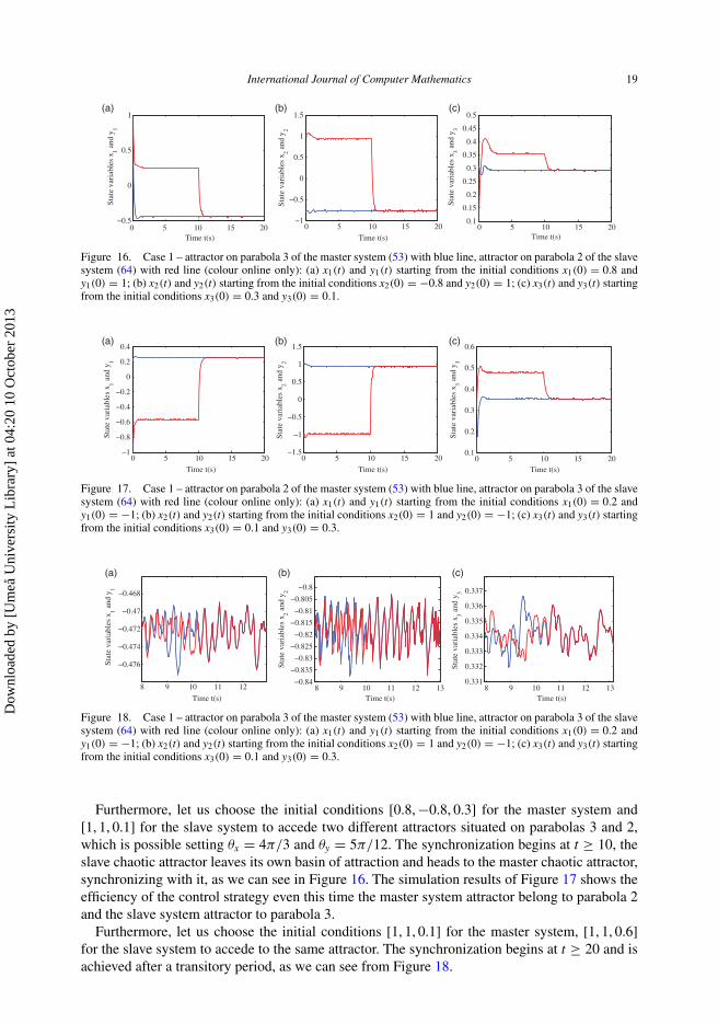
Figure 16. Case 1 – attractor on parabola 3 of the master system (53) with blue line, attractor on parabola 2 of the slavesystem (64) with red line (colour online only): (a) x1(t) and y1(t) starting from the initial conditions x1(0) = 0.8 andy1(0) = 1; (b) x2(t) and y2(t) starting from the initial conditions x2(0) = −0.8 and y2(0) = 1; (c) x3(t) and y3(t) startingfrom the initial conditions x3(0) = 0.3 and y3(0) = 0.1.
(a) (b) (c)
0 5 10 15 20−1
−0.8
−0.6
−0.4
−0.2
0
0.2
0.4
Time t(s)
Stat
e va
riab
les
x 1 and
y1
0 5 10 15 20−1.5
−1
−0.5
0
0.5
1
1.5
Time t(s)
Stat
e va
riab
les
x 2 and
y2
0 5 10 15 200.1
0.2
0.3
0.4
0.5
0.6
Time t(s)
Stat
e va
riab
les
x 3 and
y3
Figure 17. Case 1 – attractor on parabola 2 of the master system (53) with blue line, attractor on parabola 3 of the slavesystem (64) with red line (colour online only): (a) x1(t) and y1(t) starting from the initial conditions x1(0) = 0.2 andy1(0) = −1; (b) x2(t) and y2(t) starting from the initial conditions x2(0) = 1 and y2(0) = −1; (c) x3(t) and y3(t) startingfrom the initial conditions x3(0) = 0.1 and y3(0) = 0.3.
(a) (b) (c)
8 9 10 11 12
−0.476
−0.474
−0.472
−0.47
−0.468
Time t(s)
Stat
e va
riab
les
x 1 and
y1
8 9 10 11 12 13−0.84
−0.835
−0.83
−0.825
−0.82
−0.815
−0.81
−0.805
−0.8
Time t(s)
Stat
e va
riab
les
x 2 and
y2
8 9 10 11 12 130.331
0.332
0.333
0.334
0.335
0.336
0.337
Time t(s)
Stat
e va
riab
les
x 3 and
y3
Figure 18. Case 1 – attractor on parabola 3 of the master system (53) with blue line, attractor on parabola 3 of the slavesystem (64) with red line (colour online only): (a) x1(t) and y1(t) starting from the initial conditions x1(0) = 0.2 andy1(0) = −1; (b) x2(t) and y2(t) starting from the initial conditions x2(0) = 1 and y2(0) = −1; (c) x3(t) and y3(t) startingfrom the initial conditions x3(0) = 0.1 and y3(0) = 0.3.
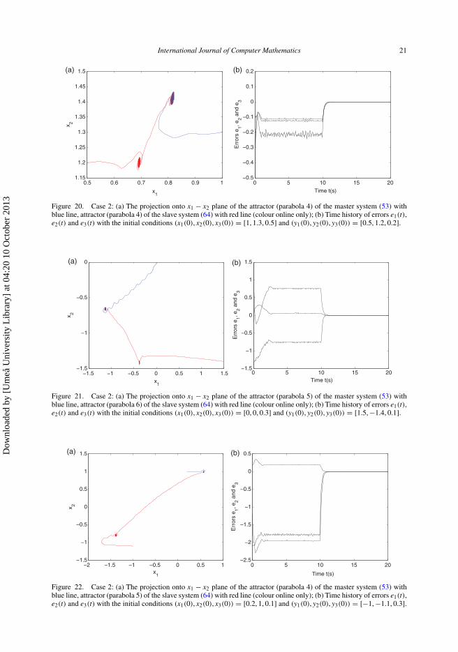
Furthermore, let us choose the initial conditions [0.8, −0.8, 0.3] for the master system and[1, 1, 0.1] for the slave system to accede two different attractors situated on parabolas 3 and 2,which is possible setting θx = 4π/3 and θy = 5π/12. The synchronization begins at t ≥ 10, theslave chaotic attractor leaves its own basin of attraction and heads to the master chaotic attractor,synchronizing with it, as we can see in Figure 16. The simulation results of Figure 17 shows theefficiency of the control strategy even this time the master system attractor belong to parabola 2and the slave system attractor to parabola 3.
Furthermore, let us choose the initial conditions [1, 1, 0.1] for the master system, [1, 1, 0.6]for the slave system to accede to the same attractor. The synchronization begins at t ≥ 20 and isachieved after a transitory period, as we can see from Figure 18.
Dow
nloa
ded
by [
Um
eå U
nive
rsity
Lib
rary
] at
04:
20 1
0 O
ctob
er 2
013
20 C. Morel et al.
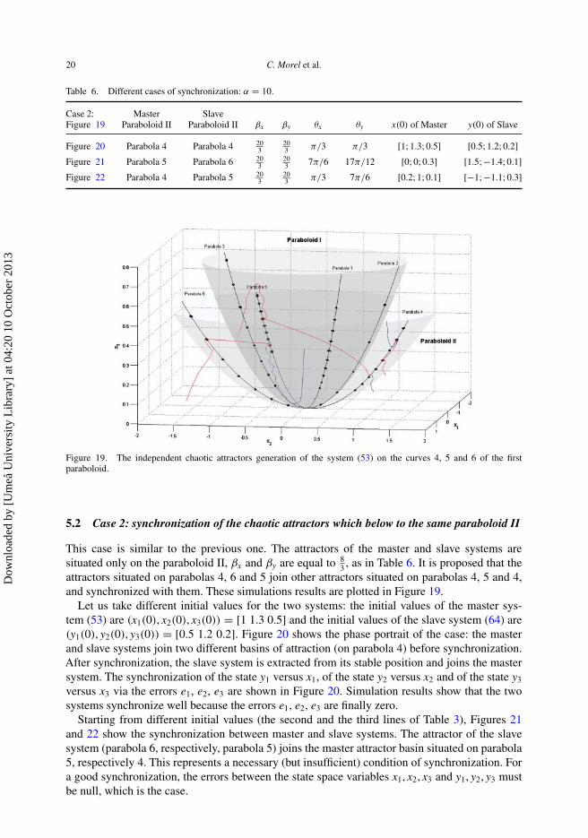
Table 6. Different cases of synchronization: α = 10.
Case 2: Master SlaveFigure 19 Paraboloid II Paraboloid II βx βy θx θy x(0) of Master y(0) of Slave
Figure 20 Parabola 4 Parabola 4 203
203 π/3 π/3 [1; 1.3; 0.5] [0.5; 1.2; 0.2]
Figure 21 Parabola 5 Parabola 6 203
203 7π/6 17π/12 [0; 0; 0.3] [1.5; −1.4; 0.1]
Figure 22 Parabola 4 Parabola 5 203
203 π/3 7π/6 [0.2; 1; 0.1] [−1; −1.1; 0.3]
Figure 19. The independent chaotic attractors generation of the system (53) on the curves 4, 5 and 6 of the firstparaboloid.
5.2 Case 2: synchronization of the chaotic attractors which below to the same paraboloid II
This case is similar to the previous one. The attractors of the master and slave systems aresituated only on the paraboloid II, βx and βy are equal to 8
3 , as in Table 6. It is proposed that theattractors situated on parabolas 4, 6 and 5 join other attractors situated on parabolas 4, 5 and 4,and synchronized with them. These simulations results are plotted in Figure 19.
Let us take different initial values for the two systems: the initial values of the master sys-tem (53) are (x1(0), x2(0), x3(0)) = [1 1.3 0.5] and the initial values of the slave system (64) are(y1(0), y2(0), y3(0)) = [0.5 1.2 0.2]. Figure 20 shows the phase portrait of the case: the masterand slave systems join two different basins of attraction (on parabola 4) before synchronization.After synchronization, the slave system is extracted from its stable position and joins the mastersystem. The synchronization of the state y1 versus x1, of the state y2 versus x2 and of the state y3
versus x3 via the errors e1, e2, e3 are shown in Figure 20. Simulation results show that the twosystems synchronize well because the errors e1, e2, e3 are finally zero.
Starting from different initial values (the second and the third lines of Table 3), Figures 21and 22 show the synchronization between master and slave systems. The attractor of the slavesystem (parabola 6, respectively, parabola 5) joins the master attractor basin situated on parabola5, respectively 4. This represents a necessary (but insufficient) condition of synchronization. Fora good synchronization, the errors between the state space variables x1, x2, x3 and y1, y2, y3 mustbe null, which is the case.
Dow
nloa
ded
by [
Um
eå U
nive
rsity
Lib
rary
] at
04:
20 1
0 O
ctob
er 2
013
International Journal of Computer Mathematics 21
0.5 0.6 0.7 0.8 0.9 11.15
1.2
1.25
1.3
1.35
1.4
1.45
1.5
x1
x 2(a)
0 5 10 15 20−0.5
−0.4
−0.3
−0.2
−0.1
0
0.1
0.2
Time t(s)
Err
ors
e 1, e2 a
nd e
3
(b)
Figure 20. Case 2: (a) The projection onto x1 − x2 plane of the attractor (parabola 4) of the master system (53) withblue line, attractor (parabola 4) of the slave system (64) with red line (colour online only); (b) Time history of errors e1(t),e2(t) and e3(t) with the initial conditions (x1(0), x2(0), x3(0)) = [1, 1.3, 0.5] and (y1(0), y2(0), y3(0)) = [0.5, 1.2, 0.2].
(a) (b)
−1.5 −1 −0.5 0 0.5 1 1.5−1.5
−1
−0.5
0
x1
x 2
0 5 10 15 20−1.5
−1
−0.5
0
0.5
1
1.5
Time t(s)
Err
ors
e 1, e2 a
nd e
3
Figure 21. Case 2: (a) The projection onto x1 − x2 plane of the attractor (parabola 5) of the master system (53) withblue line, attractor (parabola 6) of the slave system (64) with red line (colour online only); (b) Time history of errors e1(t),e2(t) and e3(t) with the initial conditions (x1(0), x2(0), x3(0)) = [0, 0, 0.3] and (y1(0), y2(0), y3(0)) = [1.5, −1.4, 0.1].
(a) (b)
−2 −1.5 −1 −0.5 0 0.5 1−1.5
−1
−0.5
0
0.5
1
1.5
x1
x 2
0 5 10 15 20−2.5
−2
−1.5
−1
−0.5
0
0.5
Time t(s)
Err
ors
e 1, e2 a
nd e
3
Figure 22. Case 2: (a) The projection onto x1 − x2 plane of the attractor (parabola 4) of the master system (53) withblue line, attractor (parabola 5) of the slave system (64) with red line (colour online only); (b) Time history of errors e1(t),e2(t) and e3(t) with the initial conditions (x1(0), x2(0), x3(0)) = [0.2, 1, 0.1] and (y1(0), y2(0), y3(0)) = [−1, −1.1, 0.3].
Dow
nloa
ded
by [
Um
eå U
nive
rsity
Lib
rary
] at
04:
20 1
0 O
ctob
er 2
013

22 C. Morel et al.
Figure 23. The independent chaotic attractors generation of the system (53) on the curves 1, 2 and 3 of the first paraboloid.The independent chaotic attractors generation of the system (53) on the curves 4, 5 and 6 of the second paraboloid.
Table 7. Different cases of synchronization: α = 10.
Case 3: Master SlaveFigure 23 Paraboloid I Paraboloid II βx βy θx θy x(0) of Master y(0) of Slave
Figure 24 Parabola 1 Parabola 5 83
203 π/6 7π/6 [1; −0.2; 0.3] [−1.5; −0.8; 0.7]
Figure 25 Parabola 3 Parabola 6 83
203 4π/3 17π/12 [0.1; −1; 0.3] [1; −1.5; 0.1]
Figure 26 Parabola 2 Parabola 4 83
203 5π/12 π/3 [0.3; 1; 0.5] [−1; 1.5; 0.2]
5.3 Case 3: synchronization of the chaotic attractors which belong to different paraboloids(paraboloid I of master attractor and paraboloid II of slave attractor)
Let us consider that the chaotic attractors to be synchronized belong to two different paraboloids:paraboloid I of master attractor and paraboloid II of slave attractor, as in Figure 23. Consequently,βx and βy take different values as in Table 7. The simulation results of the slave system attractorssituated on the paraboloid II (the parabolas 5, 6 and 4) which join other master system attractorssituated on the paraboloid I (parabolas 1, 5 and 6) are plotted in Figure 23.
Starting from the initial conditions (x1(0), x2(0), x3(0)) = [1, −0.2, 0.3], the blue trajectoryof the master system attractor, after a short transient response, remains inside its own basinon the paraboloid I, as in Figure 24. In the same figure, the red trajectory of the slave systemattractor arrives on the chaotic attractor basin, on the paraboloid II, starting from the initialconditions (y1(0), y2(0), y3(0)) of [−1.5, −0.8, 0.7]. The two generated attractors are disjunct andthe trajectory of each attractor remains inside its own basin without switching to the neighbouringattractor basin. Despite the fact that, the attractors are situated on different paraboloid, adding thecoupling terms u1, u2 and u3 of Equation (68) to the slave system (64), (y1, y2, y3) lead to (x1, x2, x3)
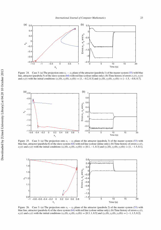
for t ≥ 10. The errors e1, e2 and e3 are canceled. This means that the chaos synchronizationbetween the master and the slave systems can be achieved. Similar cases are presented in Figures 25and 26, for two other initial conditions of Table 7.
Dow
nloa
ded
by [
Um
eå U
nive
rsity
Lib
rary
] at
04:
20 1
0 O
ctob
er 2
013
International Journal of Computer Mathematics 23
−1.5 −1 −0.5 0 0.5 1−0.8
−0.6
−0.4
−0.2
0
0.2
0.4
0.6
x1
x 2(a)
0 5 10 15 20−2.5
−2
−1.5
−1
−0.5
0
0.5
Time t(s)
Err
ors
e 1, e2 a
nd e
3
(b)
Figure 24. Case 3: (a) The projection onto x1 − x2 plane of the attractor (parabola 1) of the master system (53) with blueline, attractor (parabola 5) of the slave system (64) with red line (colour online only); (b) Time history of errors e1(t), e2(t)and e3(t) with the initial conditions (x1(0), x2(0), x3(0)) = [1, −0.2, 0.3] and (y1(0), y2(0), y3(0)) = [−1.5, −0.8, 0.7].
−0.6 −0.4 −0.2 0 0.2 0.4 0.6 0.8 1−1.5
−1.4
−1.3
−1.2
−1.1
−1
−0.9
−0.8
x1
x 2
(a)
0 5 10 15 20−0.6
−0.4
−0.2
0
0.2
0.4
0.6
0.8
1
Time t(s)
Err
ors
e 1, e2 a
nd e
3
(b)
Figure 25. Case 3: (a) The projection onto x1 − x2 plane of the attractor (parabola 3) of the master system (53) withblue line, attractor (parabola 6) of the slave system (64) with red line (colour online only); (b) Time history of errors e1(t),e2(t) and e3(t) with the initial conditions (x1(0), x2(0), x3(0)) = [0.1, −1, 0.3] and (y1(0), y2(0), y3(0)) = [1, −1.5, 0.1].
−1 −0.8 −0.6 −0.4 −0.2 0 0.2 0.4 0.6 0.80.9
1
1.1
1.2
1.3
1.4
1.5
x1
x 2
0 5 10 15 20−1.4
−1.2
−1
−0.8
−0.6
−0.4
−0.2
0
0.2
0.4
0.6
Time t(s)
Err
ors
e 1, e2 a
nd e
3
Figure 26. Case 3: (a) The projection onto x1 − x2 plane of the attractor (parabola 2) of the master system (53) withblue line, attractor (parabola 4) of the slave system (64) with red line (colour online only); (b) Time history of errors e1(t),e2(t) and e3(t) with the initial conditions (x1(0), x2(0), x3(0)) = [0.3, 1, 0.5] and (y1(0), y2(0), y3(0)) = [−1, 1.5, 0.2].
Dow
nloa
ded
by [
Um
eå U
nive
rsity
Lib
rary
] at
04:
20 1
0 O
ctob
er 2
013

24 C. Morel et al.
Figure 27. The independent chaotic attractors generation of the system (53) on the curves 1, 2 and 3 of the first paraboloid.The independent chaotic attractors generation of the system (53) on the curves 4, 5 and 6 of the second paraboloid.
Table 8. Different cases of synchronization: α = 10.
Case 4: Master SlaveFigure 27 Paraboloid II Paraboloid I βx βy θx θy x(0) of Master y(0) of Slave
Figure 28 Parabola 5 Parabola 1 203
83 7π/6 π/6 [0.3; 0.2; 0.4] [0.1; −0.3; 0.45]
Figure 29 Parabola 6 Parabola 3 203
83 17π/12 4π/3 [1.8; −1; 0.2] [1.5; −1.25; 0.55]
Figure 30 Parabola 4 Parabola 2 203
83 π/3 5π/12 [1.2; 1; 0.1] [−1; 1; 0.3]
5.4 Case 4: synchronization of the chaotic attractors which belong to different paraboloids(paraboloid II of master attractor and paraboloid I of slave attractor)
Let us take the chaotic attractors belong to paraboloid I of slave attractor and paraboloid II ofmaster attractor as in Figure 27, which βx = 20
3 and βy = 83 as in Table 8. The simulation results
of the slave system attractors situated on the paraboloid I (parabolas 1, 3 and 2) which jointother master system attractors situated on the paraboloid II (parabolas 5, 6 and 4) are plotted inFigure 27.
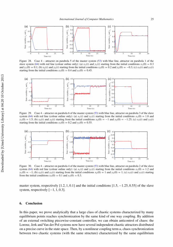
Starting from the initial conditions (y1(0), y2(0), y3(0)) = [0.1, −0.3, 0.45], the red trajectory ofthe slave system attractor, after a short transient response, remains inside its own basin. Figure 28presents the time response of the y1, y2, y3 state space variables before synchronization (withoutthe coupling term u). Starting from the initial conditions (x1(0), x2(0), x3(0)) of [0.3, 0.2, 0.4],the blue trajectory of the master system attractor arrives on an other basin of attraction as inFigure 28. The disjunct generated attractors remain inside its own basin without switching tothe neighbouring attractor basin. Adding the u coupling term of Equation (68) to the slave sys-tem (64), (y1, y2, y3) lead to (x1, x2, x3) as in Figure 28, for t ≥ 10. This means that the chaossynchronization between the master and the slave systems can be achieved. Similar results canbe observed in Figure 29, respectively, Figure 30 for the initial conditions [1.8, −1, 0.2] of the
Dow
nloa
ded
by [
Um
eå U
nive
rsity
Lib
rary
] at
04:
20 1
0 O
ctob
er 2
013
International Journal of Computer Mathematics 25
0 5 10 15 20−1.5
−1
−0.5
0
0.5
1
Time t(s)
Stat
e va
riab
les
x 1 and
y1
(a)
0 5 10 15 20−0.8
−0.6
−0.4
−0.2
0
0.2
0.4
0.6
Time t(s)
Stat
e va
riab
les
x 2 and
y2
(b)
0 5 10 15 200
0.1
0.2
0.3
0.4
0.5
Time t(s)
Stat
e va
riab
les
x 3 and
y3
(c)
Figure 28. Case 4 – attractor on parabola 5 of the master system (53) with blue line, attractor on parabola 1 of theslave system (64) with red line (colour online only): (a) x1(t) and y1(t) starting from the initial conditions x1(0) = 0.3and y1(0) = 0.1; (b) x2(t) and y2(t) starting from the initial conditions x2(0) = 0.2 and y2(0) = −0.3; (c) x3(t) and y3(t)starting from the initial conditions x3(0) = 0.4 and y3(0) = 0.45.
0 5 10 15 20−1
−0.5
0
0.5
1
1.5
2
Time t(s)
Stat
e va
riab
les
x 1 and
y1
(a)
0 5 10 15 20−1.3
−1.2
−1.1
−1
−0.9
−0.8
Time t(s)
Stat
e va
riab
les
x 2 and
y2
(b)
0 5 10 15 200.1
0.2
0.3
0.4
0.5
0.6
0.7
0.8
Time t(s)St
ate
vari
able
s x 3 a
nd y
3
(c)
Figure 29. Case 4 – attractor on parabola 6 of the master system (53) with blue line, attractor on parabola 3 of the slavesystem (64) with red line (colour online only): (a) x1(t) and y1(t) starting from the initial conditions x1(0) = 1.8 andy1(0) = 1.5; (b) x2(t) and y2(t) starting from the initial conditions x2(0) = −1 and y2(0) = −1.25; (c) x3(t) and y3(t)starting from the initial conditions x3(0) = 0.2 and y3(0) = 0.55.
0 5 10 15 20−1
−0.5
0
0.5
1
1.5
Time t(s)
Stat
e va
riab
les
x 1 and
y1
(a)
0 5 10 15 200.9
0.95
1
1.05
1.1
1.15
Time t(s)
Stat
e va
riab
les
x 2 and
y2
(b)
0 5 10 15 200.1
0.15
0.2
0.25
0.3
0.35
0.4
0.45
0.5
Time t(s)
Stat
e va
riab
les
x 3 and
y3
(c)
Figure 30. Case 4 – attractor on parabola 4 of the master system (53) with blue line, attractor on parabola 2 of the slavesystem (64) with red line (colour online only): (a) x1(t) and y1(t) starting from the initial conditions x1(0) = 1.2 andy1(0) = −1; (b) x2(t) and y2(t) starting from the initial conditions x2(0) = 1 and y2(0) = 1; (c) x3(t) and y3(t) startingfrom the initial conditions x3(0) = 0.1 and y3(0) = 0.3.
master system, respectively [1.2, 1, 0.1] and the initial conditions [1.5, −1.25, 0.55] of the slavesystem, respectively [−1, 1, 0.3].
6. Conclusion
In this paper, we prove analytically that a large class of chaotic systems characterized by manyequilibrium points reaches synchronization by the same kind of one way coupling. By additionof an external switching piecewise-constant controller, we can obtain anticontrol of chaos: theLorenz, Jerk and Van der Pol systems now have several independent chaotic attractors distributedon a precise curve in the state space. Then, by a nonlinear coupling term u, chaos synchronizationbetween two chaotic systems (with the same structure) characterized by the same equilibrium
Dow
nloa
ded
by [
Um
eå U
nive
rsity
Lib
rary
] at
04:
20 1
0 O
ctob
er 2
013
26 C. Morel et al.
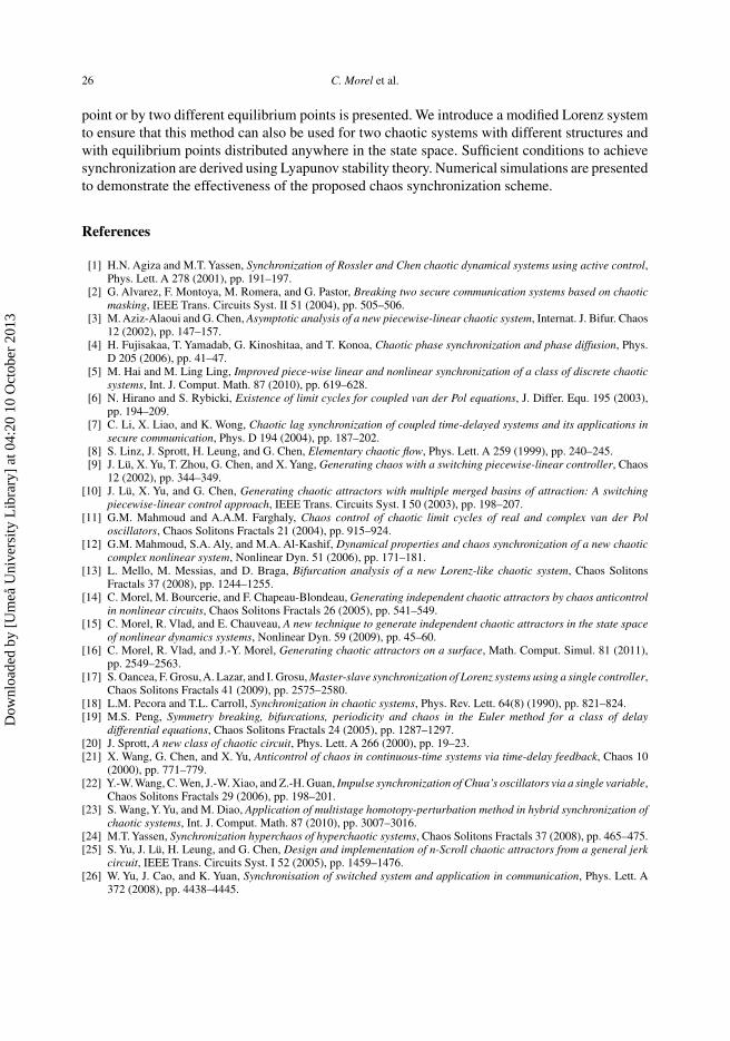
point or by two different equilibrium points is presented. We introduce a modified Lorenz systemto ensure that this method can also be used for two chaotic systems with different structures andwith equilibrium points distributed anywhere in the state space. Sufficient conditions to achievesynchronization are derived using Lyapunov stability theory. Numerical simulations are presentedto demonstrate the effectiveness of the proposed chaos synchronization scheme.
References
[1] H.N. Agiza and M.T. Yassen, Synchronization of Rossler and Chen chaotic dynamical systems using active control,Phys. Lett. A 278 (2001), pp. 191–197.
[2] G. Alvarez, F. Montoya, M. Romera, and G. Pastor, Breaking two secure communication systems based on chaoticmasking, IEEE Trans. Circuits Syst. II 51 (2004), pp. 505–506.
[3] M. Aziz-Alaoui and G. Chen, Asymptotic analysis of a new piecewise-linear chaotic system, Internat. J. Bifur. Chaos12 (2002), pp. 147–157.
[4] H. Fujisakaa, T. Yamadab, G. Kinoshitaa, and T. Konoa, Chaotic phase synchronization and phase diffusion, Phys.D 205 (2006), pp. 41–47.
[5] M. Hai and M. Ling Ling, Improved piece-wise linear and nonlinear synchronization of a class of discrete chaoticsystems, Int. J. Comput. Math. 87 (2010), pp. 619–628.
[6] N. Hirano and S. Rybicki, Existence of limit cycles for coupled van der Pol equations, J. Differ. Equ. 195 (2003),pp. 194–209.
[7] C. Li, X. Liao, and K. Wong, Chaotic lag synchronization of coupled time-delayed systems and its applications insecure communication, Phys. D 194 (2004), pp. 187–202.
[8] S. Linz, J. Sprott, H. Leung, and G. Chen, Elementary chaotic flow, Phys. Lett. A 259 (1999), pp. 240–245.[9] J. Lü, X. Yu, T. Zhou, G. Chen, and X. Yang, Generating chaos with a switching piecewise-linear controller, Chaos
12 (2002), pp. 344–349.[10] J. Lü, X. Yu, and G. Chen, Generating chaotic attractors with multiple merged basins of attraction: A switching
piecewise-linear control approach, IEEE Trans. Circuits Syst. I 50 (2003), pp. 198–207.[11] G.M. Mahmoud and A.A.M. Farghaly, Chaos control of chaotic limit cycles of real and complex van der Pol
oscillators, Chaos Solitons Fractals 21 (2004), pp. 915–924.[12] G.M. Mahmoud, S.A. Aly, and M.A. Al-Kashif, Dynamical properties and chaos synchronization of a new chaotic
complex nonlinear system, Nonlinear Dyn. 51 (2006), pp. 171–181.[13] L. Mello, M. Messias, and D. Braga, Bifurcation analysis of a new Lorenz-like chaotic system, Chaos Solitons
Fractals 37 (2008), pp. 1244–1255.[14] C. Morel, M. Bourcerie, and F. Chapeau-Blondeau, Generating independent chaotic attractors by chaos anticontrol
in nonlinear circuits, Chaos Solitons Fractals 26 (2005), pp. 541–549.[15] C. Morel, R. Vlad, and E. Chauveau, A new technique to generate independent chaotic attractors in the state space
of nonlinear dynamics systems, Nonlinear Dyn. 59 (2009), pp. 45–60.[16] C. Morel, R. Vlad, and J.-Y. Morel, Generating chaotic attractors on a surface, Math. Comput. Simul. 81 (2011),
pp. 2549–2563.[17] S. Oancea, F. Grosu,A. Lazar, and I. Grosu, Master-slave synchronization of Lorenz systems using a single controller,
Chaos Solitons Fractals 41 (2009), pp. 2575–2580.[18] L.M. Pecora and T.L. Carroll, Synchronization in chaotic systems, Phys. Rev. Lett. 64(8) (1990), pp. 821–824.[19] M.S. Peng, Symmetry breaking, bifurcations, periodicity and chaos in the Euler method for a class of delay
differential equations, Chaos Solitons Fractals 24 (2005), pp. 1287–1297.[20] J. Sprott, A new class of chaotic circuit, Phys. Lett. A 266 (2000), pp. 19–23.[21] X. Wang, G. Chen, and X. Yu, Anticontrol of chaos in continuous-time systems via time-delay feedback, Chaos 10
(2000), pp. 771–779.[22] Y.-W. Wang, C. Wen, J.-W. Xiao, and Z.-H. Guan, Impulse synchronization of Chua’s oscillators via a single variable,
Chaos Solitons Fractals 29 (2006), pp. 198–201.[23] S. Wang, Y. Yu, and M. Diao, Application of multistage homotopy-perturbation method in hybrid synchronization of
chaotic systems, Int. J. Comput. Math. 87 (2010), pp. 3007–3016.[24] M.T. Yassen, Synchronization hyperchaos of hyperchaotic systems, Chaos Solitons Fractals 37 (2008), pp. 465–475.[25] S. Yu, J. Lü, H. Leung, and G. Chen, Design and implementation of n-Scroll chaotic attractors from a general jerk
circuit, IEEE Trans. Circuits Syst. I 52 (2005), pp. 1459–1476.[26] W. Yu, J. Cao, and K. Yuan, Synchronisation of switched system and application in communication, Phys. Lett. A
372 (2008), pp. 4438–4445.
Dow
nloa
ded
by [
Um
eå U
nive
rsity
Lib
rary
] at
04:
20 1
0 O
ctob
er 2
013