SYMMETRIES, INTERACTIONS AND PHASE...

SYMMETRIES, INTERACTIONS AND PHASE

TRANSITIONS

ON GRAPHENE HONEYCOMB LATTICE

by

Bitan Roy

B.Sc, University of Calcutta, 2004

M.Sc, Indian Institute of Technology-Bombay, 2006

A THESIS SUBMITTED IN PARTIAL FULFILLMENT

OF THE REQUIREMENTS FOR THE DEGREE OF

MASTER OF SCIENCE

in the Department

of

Physics

© Bitan Roy 2008

SIMON FRASER UNIVERSITY

Spring 2008

All rights reserved. This work may not be

reproduced in whole or in part, by photocopy

or other means, without the permission of the author.

APPROVAL

Name: I3itan Roy

Degree: l\Iastcr of Scicncc

Title of thesis: Symmetries, Interactions and Phasc Transitions on Graphcnc

Honeycomh Lattice

Examining Committee: Dr. Karen Kavanagh

Chair

Dr. Igor Hcrhut, Senior Supervisor

Dr. l\Ialcolm Kcnnett, Supervisor

Dr. Howard TrotticL SupervisoL

01', Levan Pogosian, SFU Examiner

Date Approved:

n

SIMON FRASER UNIVERSITYLIBRARY

Declaration ofPartial Copyright LicenceThe author, whose copyright is declared on the title page of this work, has grantedto Simon Fraser University the right to lend this thesis, project or extended essayto users of the Simon Fraser University Library, and to make partial or singlecopies only for such users or in response to a request from the library of any otheruniversity, or other educational institution, on its own behalf or for one of its users.

The author has further granted permission to Simon Fraser University to keep ormake a digital copy for use in its circulating collection (currently available to thepublic at the "Institutional Repository" link of the SFU Library website<www.lib.sfu.ca> at: <http://ir.lib.sfu.calhandle/1892/112>) and, without changingthe content, to translate the thesis/project or extended essays, if technicallypossible, to any medium or format for the purpose of preservation of the digitalwork.

The author has further agreed that permission for multiple copying of this work forscholarly purposes may be granted by either the author or the Dean of GraduateStudies.

It is understood that copying or pUblication of this work for financial gain shall notbe allowed without the author's written permission.

Permission for pUblic performance, or limited permission for private scholarly use,of any multimedia materials forming part of this work, may have been granted bythe author. This information may be found on the separately cataloguedmultimedia material and in the signed Partial Copyright Licence.

While licensing SFU to permit the above uses, the author retains copyright in thethesis, project or extended essays, including the right to change the work forsubsequent purposes, including editing and publishing the work in whole or inpart, and licensing other parties, as the author may desire.

The original Partial Copyright Licence attesting to these terms, and signed by thisauthor, may be found in the original bound copy of this work, retained in theSimon Fraser University Archive.

Simon Fraser University LibraryBumaby, BC, Canada

Revised: Fall 2007

Abstract

Graphene, a monolayer of graphite, opened a new frontier in physics with reduced dimen

sionality. Due to the Dirac nature of the quasi particles it exhibits interesting experimental

phenomena. It is believed that electron-electron interactions also play important role in

graphene. We derive here a generalized theory of short ranged interactions consistent with

the various discrete symmetries present on the lattice. Restrictions on the theory imposed

by the atomic limit are also discussed. Within the framework of this model we calculated

the beta functions governing the renormalization flow of the couplings to sub-leading order

in liN. Our calculations show that charge density wave and anti-ferromagnetic quantum

critical points are in the Gross-Neveu universality class even beyond mean-field level. There

after we use the extended Hubbard model to extract the phase diagram. It shows that the

semimetallic ground state is stabilized once we include corrections to sub-leading order in

liN.

III

Acknowledgments

During one and half years at Simon Fraser University many people have supported me to

get through the process of acquiring a Master's degree. It is my pleasure to acknowledge

them.

First of all, I am indebted to Prof. Igor Herbut for his scientific and moral support during

the time I spent at Simon Fraser University. He introduced me to the physics of graphene

which was a completely new area for me at the time I started my Master's studies. He

was a brilliant supervisor and his ideas profoundly influenced my work during this period.

Thanks Igor!

I would like to express my gratitude to Dr. Vladimir Juricic, a post-doc in Igor's group,

with whom I worked for a year at Simon Fraser University. It was a great pleasure working

with Vladimir whose ideas had a great impact on the work presented in this thesis.

During my stay at Simon Fraser I had a great pleasure to meet Kamran Kaveh-Maryan,

who was a graduate student in the group. I am thankful to Kamran for his help in useful

discussion and also for some technical advice. A special thanks to Kamran for his help

concerning layout of the thesis. I also want to thank Himadri Sekhar Ganguli, who was a

graduate student in Department of Mathematics, for his constructive discussions on several

issues which stimulated me to develop a profound mathematical background.

It is my great pleasure to thank the faculty members who have taught courses during

my Master's studies. Their scientific attitude affected my thinking always in a positive way.

At the same time I want to express my gratitude to Dr. Howard Trottier and Dr. Malcolm

Kennett for their patience during several discussion which boosted my enthusiasm towards

theoretical physics a lot.

During my stay at Simon Fraser University it was my great pleasure to meet Peter

Smith, Sara Sadeghi, as well as Mathew Downton. Sharing office with Peter and Sara was

IV

also a great experience.

Last, but not least I would like to thank my parents for providing moral support during

my entire academic period.

v

Contents

Approval ii

Abstract iii

Acknowledgments iv

Contents vi

List of Figures viii

1 Introduction

1.1 Outline of the work.

2 Symmetries and interactions in graphene honeycomb lattice

2.1 Free Lagrangian .

2.2 Interactions and symmetries.

2.2.1 "Mirror" symmetry (5)

2.2.2 Time reversal symmetry (TRS)

2.3 Translational invariance

2.4 Parity symmetry ....

2.5 Atomic limit and interactions

2.6 Outline of the work .

3 Renormalization and phase transition

3.1 Wilson's one loop renormalization

3.2 Phase transitions . . . . .

3.3 Extended Hubbard model

VI

1

6

8

8

10

11

12

15

16

18

21

22

23

25

28

4 Conclusions 34

A Momentum shell integration in one loop Wilsonian renormalization 37

B Flow equations 39

C Susceptibilities of Dirac fermions in (2+1)-dimensions 44

Bibliography 47

Vll

List of Figures

1.1 Various allotropes of carbon. . . . . . . . 2

1.2 QHE in single layer and bi-layer graphene 3

1.3 Lattice structure of graphene honeycom lattice 4

1.4 Brillouin zone of honeycomb lattice. . . . . . 5

1.5 Conical energy dispersion at the Dirac point 7

2.1 Kekule pattern on graphene honeycomb lattice due to anisotropic hopping. 18

2.2 Basic building block of the Kekule Pattern on honeycomb lattice . . . . .. 19

3.1 Mean-field flow diagram in (ga, gc) attractive plane . . 26

3.2 Flow diagram for in (ga, gc) attractive plane for N = 2 27

3.3 Phase diagram for the extended Hubbard model 32

A.l Particle-hole and particle-particle diagrams at the one loop level without spin

degrees of freedom . . . . . . . . . . . . . . . . . . . . . . . . . . . . . . . .. 38

B.l Particle-particle and particle-hole diagrams at the one-loop level with spin

degrees of freedom . . . . . . . . . . . . . . . . . . . . . . . . . . . . . . . " 43

viii

Chapter 1

Introduction

Carbon is the prime material for life on the planet and the basis of the entire organic chem

istry. Because of the flexibility in its bonding, carbon-based systems show a large variety

of structures with versatile physical properties. Depending on the dimensionality of the

system, physical properties of carbon-based materials vary widely. Among the systems with

only carbon atoms, graphene is a two-dimensional (2D) allotrope of carbon. In graphene,

carbon atoms are arranged on a honeycomb structure made out of hexagons. This struc

ture is similar to benzene rings stripped of hydrogen atoms. Graphite, which became well

known to mankind after the invention of lead pencil in 1564, is a 3D allotrope of carbon

Fig. [1.1]. The usefulness of graphite as a writing instrument comes from the fact that

graphite is made out of stacks of graphene layers, weakly coupled by van del' Waals forces.

Hence, one produces various layers of graphene on paper while writing on it. Although one

produces multiple layers of graphene on paper while writing, it took 440 years to isolate a

single layer. Graphene, a 2D layer of graphite was first fabricated successfully by Novoselov

et al. [1]. The reason behind this delay is not a lack of experimental tools to produce an

atomicly thick layer of graphene but rather the persistence to confirm success [2]. Thin

graphite or Graphene was eventually spotted due to subtle optical effects that it produces

on top of a Si02 substrate [1].

It was P.R. Wallace [3] who first studied the band structures of graphene and discovered

the semi-metallic nature of this material. Further theoretical developments came up with

the most interesting properties that its low energy excitations are massless, chiral, Dirac

fermions. This prescription, valid only on energy scales much smaller than the band width,

1

Introduction 2

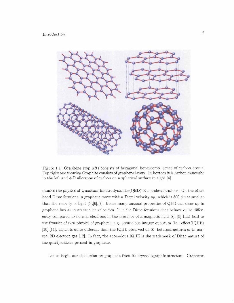
Figure 1.1: Graphene (top left) consists of hexagonal honeycomb lattice of carbon atoms.Top right one showing Graphite consists of graphene layers. In bottom it is carbon nanotubein the left and 3-D allotrope of carbon on a spherical surface in right [4].

mimics the physics of Quantum Electrodynamics(QED) of massless fermions. On the other

hand Dirac fermions in graphene move with a Fermi velocity 'up, which is 300 times smaller

than the velocity of light [5]'[6]'[7]. Hence many unusual properties of QED can show up in

graphene but at much smaller velocities. It is the Dirac fermions that behave quite differ

ently compared to normal electrons in the presence of a magnetic field [8], [9] tha.t lead to

the frontier of new physics of graphene, e.g. anomalous integer quantum Hall effect(IQHE)

[10],[11], which is quite different than the IQHE observed on Si- heterostructures or in nor

mal 2D electron gas [12]. In fact, the anomalous IQHE is the trademark of Dirac nature of

the quasiparticles present in graphene.

Let us begin our discussion on graphene from its crystallographic structure. Graphene

Introduction 3

-I/?

3tll

1/2 ~~

o t_~'H- -- ----- -- -_. -. ---- .. --- - - -1/?

------------..J -3'2

- ------------------r- -51'

-? 0 ? !.

/I ( Ol? COy.;',

n( Ol?cm~')

.2 4. -,-2

--,"" t4e2/h) 7/2

d /3 'oJ/2

2

5

o

10 -,1 -2

Figure 1.2: Figure shows the anomalous quantum hall pla.teaus for single layer graphcne.Inset diagram is for bila.yer graphene [10].

indeed is made out of carbon atoms 8nanged in hexagonal honeycomb lattice as shown in

Fig.[lA]. The Bravais la.ttice of this structure is the triangular lattice and the honeycomb

lattice be described as two interlocked triangular sub-lattices labelled A and B depicted in

Fig. [1.2]. The sub-lattice A is generated by the linear combination of the basis vectors

al = (V3, -l)a, al = (0, l)a whereas the sub-lattice B is then at B = .1 -+ b, with bbeing

b~ = (1/V3, 1)a/2, b~ = (1/V3, -1)a/2, or b~ = (-1/V3, O)a, where a is the lattice spacing

= 2.5A. Therefore the reciprocal lattice in momentum space is described by the vectors

Rl = ~o. (1,0) and R2 = ~o( ~, 1) and hence the Brillouin zone is also a hexagon.

Let us now consider the electrons present on the honeycomb lattice and review their

behavior on it. An excellent model to start with is the tight binding model which mimics

almost all the relevant physics. In this model only the nearest-neighbor hopping is taken

into a.ccount. On the other hand probability amplitude for next nearest neighbor hopping

and further remote hopping decays exponentially and therefore can be neglected. We further

consider this model for a general diatomic system with different energies of electrons localized

Introduction

B

B

4

Figure 1.3: Lattice structure of graphene honeycomb lattice showing sublattices A(red) andB(blue) with different lattice vectors that generate two interlocked triangular sublattices.

on site A and B. Let t be the hopping parameter related to the probability amplitude for

electron transfer among nearest-neighbor sites and (3 be the difference in energies of electrons

localized on site A and B. An example of a layered diatomic material described by this lattice

is boron nitride [13]. The electronic structure of Carbon is 1s22s22p 2. Therefore it has 4

electrons in the outer shell. Out of these 3 electrons form bonds with nearest neighbor sites

by Sp2 hybridization and the fourth electron in the pz orbital can hop through the system.

Due to strong overlap of the "lave functions on nearest neighbor sites t is large for graphene

rv 2.5 eV. Therefore the Hamiltonian corresponding to the model reads

H t = - t LA,i,er=±l

+ (3 L [uert(A)uer(A) - vert(A + b~)ver(A + b~)]

A,er=±l

(1.1 )

-t( cikb~ + eikb<; + C1kb3 ) )

-(3

where U t and U (v t and v) are the electron creation and annihilation operators on the sub

lattice A (B) of the honeycomb lattice. Ignoring the spin for the sake of simplicity, we can

write down the Hamiltonian as

Jd2k t ~ t-:H t = (27f)2 (u (k), v (k))

x ( -t(eik'~ + :'k'; + eif.b')

x ( u(~) )v(k)

(1.2)

Introduction 5

II

/

/\- -l \

I

\

~~. .\-~ \

\ i \

~ ~}\ J }Rj\ .I \./ J I

'\ f .,.../\ /

I /.k\L ~

Figure 1.4: The Brillouin zone. The reciprocal-lattice vectors are R1 = (47f/v'3a) (1, 0) ,R~ = (47f/v'3a) (1/2, v'3/2). The degeneracy points occur at the corners ijklmn, of theBrillouin zone [14].

using the fourier transforms

j.d2k --~ ik·B ~

v(B) = (27f)2e v(k). (1.3)

Therefore within the framework of the tight binding model the energy spectrum E(k) =

±(,62 + t2leikb~ + eikb; + eikb;1 2)1/2, is doubly degenerate. With one electron per site, the

negative energy states constitute the filled valence band and positive energy states form the

empty conduction band. The separation between these bands is minimal at the zeros of

the function f(k) = (eikb~ + eikb; + eikb;), which happens to occur at the six corners of

the Brillouin zone but out of those only two at ql = (47f/v'3a) (1/2, 1/2v'3) and q?, = -ql

are non-equivalent. Hereafter we restrict our discussion to the monatomic system for which

,6 = 0 i.e. electrons on different sub-lattices have equal energy. For such a system, e.g.

graphene with carbon atoms sitting at every site, the valence and conduction bands touch

each other at these points [14]. Therefore within the frame work of the tight binding model

Introduction 6

graphene exhibits a semi-metallic ground state and a large value of t gives the semi-metallic

state extra protection against interactions. Hence only electrons near these two points take

part in the dynamics at low energies. Considering the low energy limit expansion of f(k)

about ql gives~ ~ .tV3 -i£.!<: .t i£.!<:

f(ql + k) = -1,-2-e 3 kx + z2"(e 3 - l)ky. (1.4)

A similar expansion of f(k) about q2 = -ql can be obtained by using the relation

f(q2 + k) = - J*(ql + k). (1.5)

Hence the dispersion relation w 2 = t 2 lf(kW near these two point becomes

w2 = 3t2 (kx2 + ky 2) + O(k3).4

(1.6)

Therefore the valence and the conduction bands look like linear isotopic cones near these

two points in the Imv energy limit. Thus the Hamiltonian H t in the low energy limit reduces

to

(1. 7)

where P± = ±px(Tx - Py(Ty, and (TXl (Ty are Pauli matrices. Here the frame of reference is

conveniently rotated to Px = p' (J/ q and Py = (if x f!) x if/q2, where if = ql and q2 (= -ql) are

the momenta associated with the Dirac points. Therefore the Hamiltonian H t in the low

energy limit is a Dirac-like Hamiltonian near these two points. Thus we dub these two points

Dirac points and electrons near the two Dirac points behaves like relativistic fermions. On

the other hand, if we include further remote hopping that won't affect the Dirac behavior

of the quasi-particles but the Dirac cone will be shifted towards higher energy.

1.1 Outline of the work

Therefore witlJin the framework of the tight-binding model we recognize the Dirac nature

of the pseudo-relativistic quasi particles. We hereafter exploit this feature to develop the

interacting theory of electrons on the honeycomb lattice. We will construct the interacting

theory on honeycomb lattice consistent with the discrete symmetries present on it.

Introduction 7

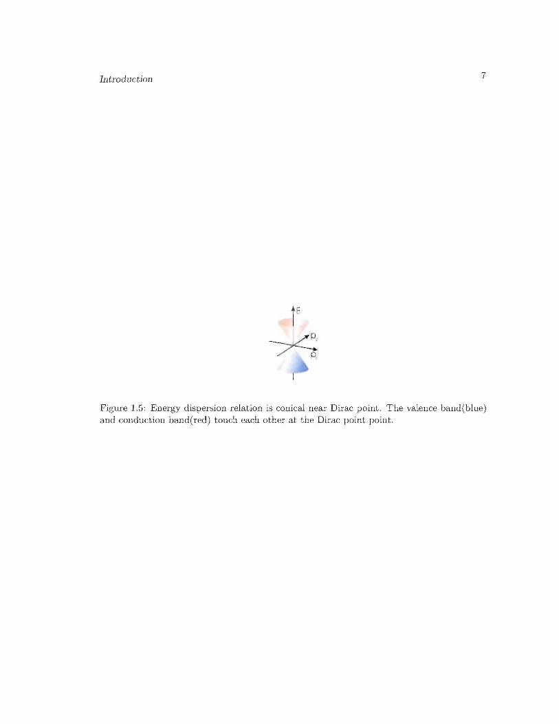
Figure 1.5: Energy dispersion relation is conical near Dirac point. The valence band(blue)a.nd conduction band(red) touch each other at the Dirac point point.

Chapter 2

Symmetries and interactions

graphene honeycomb lattice

•In

In the introductory discussion we have noticed some interesting characteristics of electrons

on graphene's honeycomb lattice, especially in the low energy regime. In that regime, we

find that electrons behave like Dirac fermions near two non-equivalent Dirac points located

at the corners of the Brillouin zone of the honeycomb lattice. Thus the electrons near these

two points have dynamical importance in the low energy sector. Therefore we construct

the free electron theory in the continuum limit which also allows us to define the so called

'valley representation' of ,- matrices by considering the electrons only near these two points.

Going beyond the free electron model we here develop the interacting theory of electrons on

honeycomb lattice consistent with the various discrete symmetries present on it. Further

more, we consider only the four-fermion interactions and spinless fermions. The restriction

on the interactions due to the 'atomic limit' is also presented here. At last, we reintroduce

the spin degrees of freedom to generalize our discussion.

2.1 Free Lagrangian

Before describing interactions on the honeycomb lattice it is useful to study the free electron

theory to define the representation for both the Dirac spinor and the matrices. Here we

8

Symmetries and interactions ...

construct the four component spinors as

9

(2.1)

Ua(ql + p,wn)

va(ql + p,wn)

U a (q2 + p,wn )

V a (Q2 + p, wn )

after conveniently rotating the frame of reference to Px = p' iffq and py = (ifx P) x if!q2 , where

if= ql and q2(= -ql) are the momenta associated with the Dirac points, T is temperature,

T is the imaginary time and W n = are the fermionic Matsubara frequencies which form a

continuum in the zero temperature limit. Hence we can write down the quantum mechanical

action corresponding to H t as

(2.2)

where

.(~) .(~)M x = -~ ~ ,lvly = ~ Ol;; .Here we have taken the Fermi velocity VF = t'f = 1 and n = kB = 1 for convenience. We

can also write Alx , My in terms of other matrices as

(2.3)

satisfying the following Clifford algebra

(2.4)

so that

Hence the quantum mechanical action at zero temperature can be written as

S = 1{3 dTJd2x L "ifiaUi, Th~a~'ljJa(x, T).o a=±l

where "ifia(x, T) = 'ljJ t (x, Tho and we define the 1 matrices as

(2.5)

(2.6)

12 (2.7)


so that they satisfy the anti-commutation relation (2.4). We further define

10

(2.8)

which anticommute with all the other,- matrices and also {'3, ,5} = O. Finally we construct

which commutes with 'J.L' f.L = 0,1,2 but anti-commutes with ,3 and ,5' Together these

define the so called 'valley representation' of, matrices. Therefore the quantum mechanical

action, S = fa liTdTdxLo, defines the free Lagrangian as

La = 2...= -;;jja'J.L 8J.L'l/Ja.a=±l

(2.9)

The free Lagrangian La obviously respects relativistic invariance. Apart from that it also

exhibits a global U(4) symmetry generated by {h, iT} ® {I, ,3, '5, '35}.

2.2 Interactions and symmetries

Let us now consider electron-electron interactions on graphene's honeycomb lattice. We will

focus here only on four fermion interactions which in general are defined by the Hamiltonian

Hint = 2...= (0:/31 V I ,8)rat r,6t r"r-y,a,,6,-y,"

(2.10)

(2.11)

where r t and rare fermionic creation and annihilation operators, satisfying the relation

{ra , rb} = 8a ,6, and the matrix element corresponding to the interaction potential V(k) is

(0:/3 I V I ,8) is given by

(0:/31 V I ,8) = JdxdY'{Ja*(x)'{J,6*(Y)V(x - Y)'{J-y(x)'{J,,(fJ).

Here we can take '(J(x) to be localized p-orbital wave-functions that belong to either A or

B sublattice. In general, there is no restriction on the overlap of the wave-functions, and

all the matrix elements (0:/3 I V I ,8) are finite. In the following we consider only short

ranged interactions, which are defined by the potential V(X) with regular Fourier component

V(k) at k = O. We further restrict the interaction potential to be a contact potential, i.e.

Symmetries and interactions ... 11

V(x - iJ) = V(x)c5(x - iJ)· Therefore at low energies we can write down the interacting

Lagrangian for spinless fermions corresponding to Hint as

(2.12)

where A and Bare 4 x 4 Hermitian matrices. Therefore the interacting Lagrangian contains

162 parameters. However, the number of parameters in Lint is restricted by the symmetries

present on the lattice. Two discrete symmetries present on the lattice are mirror symmetry

and time reversal symmetry.

2.2.1 "Mirror" symmetry (S)

The labelling of the two sublattices is arbitrary, and therefore Lint should be invariant under

the exchange of sublattice labeling (A~B)implying that Lint has to be invariant under the

exchange of components (Ui~Vi), within the same valley. In the valley representation we

recognize the mirror symmetry operator as

(~0 )S=,2 =

CJx

and thereforeu a (ql) v a (ql)

Sv a (ql) u a (Ql)

(2.13)u a (Q"2) va (Q"2)

va (Q"2) U a (Q"2)

Invariance of Lint under mirror symmetry requires both A and B to be either even, i.e.

SAS- 1 = A and SBS- 1 = B (even)

or odd, i.e

SAS~l = -A and SBS- 1 = -B (odd)

under S.


2.2.2 Time reversal symmetry (TRS)

12

Invariance of the Hamiltonian under TRS requires ItHIt -1 = H, where It is the TRS

operator, defined as It = T K. Here T is the unitary operator and K is the complex

conjugate operator. We here consider the Hamiltonian

H = irO,iPi + mI,O, (2.14)

where the mass mI arises due to the imbalance in chemical potential on two sub-lattices

A and B [?]. The mass term mI give rise to charge density wave ordering on the lattice

and thus mI is real. Therefore it is invariant under time reversal symmetry. On the other

hand time reversal symmetry of the free Hamiltonian originates in the tight binding model

from the fact that its elements are real. Recall that momentum changes sign under the

transformation ItPiIt -1 = -Pi. Therefore, invariance of H under TRS implies

{T, i,O,I} = [T, irO,2] = [T, '0] = o. (2.15)

(2.16)

Hence T E {i,n3, i,n5}. Therefore within the framework of the tight binding model with

uniform hopping time reversal symmetry is not uniquely defined. Hence we need to consider

a generalized tight binding model with anisotropic hopping defined as

3

Haniso = - L L(t + i5tr,i)U~Vf"+b~ + H.c.,rEA i=I

where

(2.17)

represents non-uniform hopping and 't' is the uniform one. Here, K± are the momenta

associated with the Dirac points K and K' respectively and G = K~ - K__ . Therefore

G couples the two non-equivalent Dirac points at K±. Let us consider the affect of the

non-uniform hopping on lattice. The non-uniform hopping can generates a so called Kekule

texture on the lattice. We will discuss this issue latter in the context of parity symmetry.

On a length scale much larger than the lattice spacing a, the Hamiltonian to the leading

order in the gradient expansion, subject to a Kekule texture is given by

(2.18)

with

(2.19)


where ± denotes the Dirac points at K± and u, v have their usual significance. Notice here

that for convenience we have chosen a different definition of the spinoI' 'lj;( f} from (2.1). The

kernel in the Hamiltonian (2.18)is defined as

0 -2iOz b.(f) 0

-2i8z 0 0 ~(f)(2.20)lCD =

~(f) 0 0 2iaz

0 b.(f} 2i8z 0

where z = x + iy and therefore az (ax - iOy )/2, where overline denotes complex con

jugation. With a Kekule structure b.(f) = b.o, the dispersion takes the simple form

€±(tf) = ±vlpF + lb.oI 2 , i.e., a single particle mass gap Ib.ol opens up. The Dirac ker

nel lCD respects time reversal symmetry originating from the real elements in tight-binding

model. Although the order parameter ~o is relaxed to be complex its phase is redundant

because the spectral mass gap is real. In fact it can be removed from the kernel (lCD) with a

chiral transformation that rotates the phases of ± species by opposite angles. On the other

hand this is not true any more if the phase in the order parameter ~(f) varies in space, and

in particular, if it contains vortices [15].

In the limit b.o= 0 the Hamiltonian Haniso reduces to

(2.21)

where Ho is the free Hamiltonian. We can also write down the free Hamiltonian in terms

of other matrices by defining

(2.22)

so that these matrices also satisfy the anti-commuting algebra (2.4). Choosing 1'0 = (jz®(jz,

one finds 1'1 = 12®(jy and 1'2 = -I2®(jx· We further chose 1'3 = (jx®(jz and 1'5 = (jyQ9(jz.This

representation of the 1'- matrices is unitarily equivalent to the valley representation, where

the transformation is generated by

(2.23)

In the continuum limit the Hamiltonian with anisotropic hopping reduces to

(2.24)


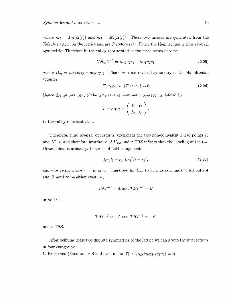
where m2 = Im(~(f}) and m3 = Re(~(f}). These two masses are generated from the

Kekule pattern on the lattice and are therefore real. Hence the Hamiltonian is time reversal

symmetric. Therefore in the valley representation the mass terms become

(2.25)

where H m = m2il'Ol'3 + m3hol's. Therefore time reversal symmetry of the Hamiltonian

requires

(2.26)

Hence the unitary part of the time reversal symmetry operator is defined by

in the valley representation.

T = hll's = (0 h),h 0

Therefore, time reversal operator T exchanges the two non-equivalent Dirac points K

and K' [4] and therefore invariance of Hint under TRS reflects that the labeling of the two

Dirac points is arbitrary. In terms of field components

(2.27)

and vice-versa, where ri = Ui or Vi. Therefore, for Lint to be invariant under TRS both A

and B need to be either even i.e.,

TAT- I = A and TBT- I = B

or odd i.e.,

TAT- I = -A and TBT- I =-B

under TRS.

After defining these two discrete symmetries of the lattice we can group the interactions

in four categories:

1. Even-even (Even under S and even under T): {I, 1'2, h01'3, hns} == A


2. Even-odd: {ir01'I, ira1'5 , irn3, ir3l'5} == B3. Odd-even:{ro, 1'3, ira1'2 , ir3l'2} == C4. Odd-odd:{rl' 1'5, irn2, ir51'2} == jj

15

Hence the interacting Lagrangian which is symmetric under mirror symmetry (8) and

TRS (It) is required to be of the following form

Lint alia2j (1/) Ai?/J) (?/J t Aj?/J) + blib2j (?/J tBi?/J) (?/J t Bj?/J)

+ CliC2j (?/J t Ci?/J) (1/) Cj?/J) + dlid2j (?/J t Di?/J) (?/J t Dj?/J)

(2.28)

Where ai, b~, cj, d~, i = 1,2 are the coupling constants. We further notice that all the

interactions e.g. the first one, alia2j(?/JtAi?/J)(?/JtAj?/J) are symmetric under the exchange of

indices i, j. Therefore the number of interactions allowed by "Mirror" symmetry and TRS

is 40.

2.3 Translational invariance

Apart from these two discrete lattice symmetries, the interactions conserve the momentum

at two Dirac points. The couplings that are allowed by the momentum conservation or

alternatively translational invariance have the form {rlr±rlr±,rtr+r~r_}, corresponding

to block-diagonal matrices in the interacting Lagrangian, while {rtr+r~r+}, corresponds

to block off diagonal matrices in the interacting Lagrangian (2.28). Here ± labels the two

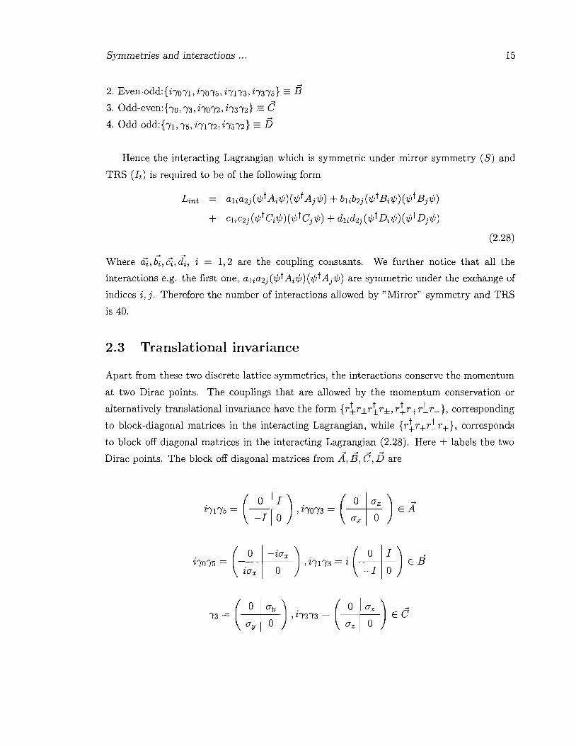
Dirac points. The block off diagonal matrices from .x, B, C, jj are

Z1'01'5 =(*-iax

) (*1). ,Z1'I1'3 = Zzax 0 -1 0

Symmetries and interactions... 16

(0 I -i(J ) ($i(J)')'5 =~ ,i/2I5 = . zED.

i(Jy I 0 -2(}"z 0

Therefore two block-diagonal matrices from each group A, B, 6, D and the remaining eight

block off-diagonal matrices altogether define the translationally invariant interacting La

grangian as

Lint 'l/Jt(al + a2l2)'l/J'l/Jt(a3 + a4l2)'l/J

+ 'l/Jt(bno + b2i')'o')'2)'l/J'l/Jt(b3/0 + b4i/O')'2)'l/J

+ 'l/J t (CI i')'O')'l + C2i/3/5 )'l/J'l/Jt (C3i/O')'1 + C4 i')'3/5)'l/J

+ 'l/Jt(dnl + d2i')'l/2)'l/J'l/Jt (d3/1 + b4i/l/2)'l/J

+ 9A'l/Jt (i/l/3 + ')'n5)'l/J'l/Jt (i/l/3 -')'l/5)'l/J

+ gB'l/Jt(i')'o')'3 + ')'O')'5)'l/J'l/Jt(i')'o')'3 -')'O')'5)'l/J

+ 9C'l/Jt (')'3 + i/5)'l/J'l/Jt(')'3 - i/5)'l/J

+ 9D'l/Jt (i/2I3 + ')'2I5)'l/J'l/Jt(i/2I3 -')'2I5)'l/J (2.29)

Hence all the symmetries present on the lattice restricts the number of allowed interactions

to 16 and this is the most general interaction allowed by symmetry. Note that Lint is

invariant under the U(l) symmetry generated by i/3/5 = (Jz®h. This is same as imposing

translational invariance and can be used as an alternative way to generate(2.29) from (2.28).

2.4 Parity symmetry

For the sake of completeness we here also examine how the interactions transform under the

parity(P). Once again let us begin with the free Hamiltonian

Ht = i/O')'iPi· (2.30)

This Hamiltonian is invariant under the parity transformation since honeycomb lattice with

uniform hopping is invariant under space inversion. Recall that the momentum changes sign

under the parity transformation, i.e.,

(2.31 )


Thus the invariance of the free Hamiltonian under parity implies

{P,irorI} = {P,iror2} = o.

There are four matrices that anti-commute with both irorl and irOr2, thus

17

(2.32)

Let us now incorporate a mass term generating from the charge density wave ordering on

lattice. We have already found that this mass in continuum limit reads as mrO. This mass

is invariant under parity also since it is real on lattice. On the other hand the charge density

wave ordering generates from the imbalance in chemical potential on the two sub-lattices,

therefore m-t - m under the parity. This imposes further restriction {P, ro} = 0, for the

Hamiltonian to be invariant under parity (P) and thus P E {iror3, irors}. Therefore, one

can define the parity operator as

P = iro(r3 cos 0 + rS sinO), (2.33)

where the parameter O(0::;O::;27f) is to be determined to define P uniquely. Note that this

definition of parity operator (P) in (2.33) is independent of representation of r- matrices.

On the other hand 0 depends on the representation. However, tight binding model with

uniform hopping restricts the scope to determine 0 uniquely. Therefore to determine 0 and

uniquely define the parity operator we impose anisotropy in the hopping amplitude [15].

Kekule pattern generating from anisotropic hopping and its transformation under space

inversion is depicted in Fig.[2.1] and Fig.[ 2.2]. The Hamiltonian with anisotropic hopping

is already defined in (2.16). Here without any loss of generality we here choose .6.(f') = .6.0 ,

where .6.0 is real. Therefore in continuum limit the Hamiltonian reads as

H = irOriPi + .6.oirors. (2.34)

The pattern (c) in Fig. [2.2] corresponds to the mass .6.oiror3 and this is invariant under

the space inversion with the inversion center located at the center of a hexagon. On the other

hand masses corresponding to (a) and (b) transforms into each other under space inversion

or parity. Therefore P.6.op-1 = .6.0 and invariance of H under the parity transformation

requireso= ~ 37f

2' 2 . (2.35)


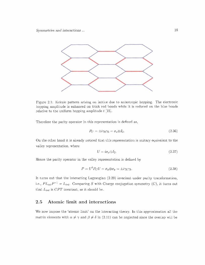
Figure 2.1: Kekule pattern arising on lattice due to anisotropic hopping. The electronichopping amplitude is enhanced on thick red bonds while it is reduced on the blue bondsrelative to the uniform hopping amplitude t [15].

Therefore the parity operator in this representation is defined as,

(2.36)

On the other hand it is already noticed that this representation is unitary equivalent to the

valley representation, where

(2.37)

Hence the parity operator in the valley representation is defined by

(2.38)

It turns out that the interacting Lag,Tangian (2.29) invariant under parity transformation,

i.e., PLintP-1 = Lint. Comparing S with Charge conjugation symmetry (C), it turns out

that Lint is CPT invariant, as it should be.

2.5 Atomic limit and interactions

We now impose the 'atomic limit' on the interacting theory. In this approximation all the

matrix elements with cy =I 'Y and j3 =I <5 in (2.11) can be neglected since the overlap will be


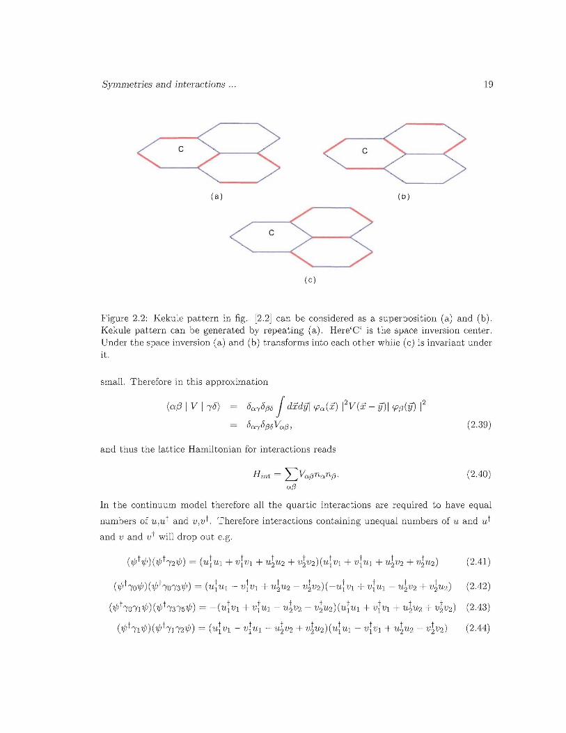
(a) (b)

19

(c)

Figure 2.2: Kekule pattern in fig. [2.2] can be considered as a superposition (a) and (b).Kekule pattern can be generated by repeating (a). Here'C' is the space inversion center.Under the space inversion (a) and (b) transforms into each other while (c) is invariant underit.

small. Therefore in this approximation

(0:131 V 1'Y fJ ) = fJ(xy6fJtj JdidYi CPaJx) 12 V(x - 77)1 CPfJ(77) 12

= Oa,Oj3O Vo:!3,

and thus the lattice Hamiltonian for interactions reads

Hint = :L:Vaj3na nj3.

a{3

(2.39)

(2.40)

In the continuum model therefore all the quartic interactions are required to have eC]ual

numbers of "U,u t and v,vt . Therefore interactions containing unequal numbers of u and ut

and v and vt will drop out e.g.

('l/J t 'Yo'l/J) (?j;t ~/O'Y31jJ) = (utu I - vtVI + U~U2 - v1V2)( _·ut VI + VtUl - U1U2 + V~"U2) (2.42)

('¢) 'YO'YI1/JKli) "I3'Y5'l/J) = - (ut VI + Vi"UI - "U1 V2 - V6 U2) ("Ut"Ul + viVI + "U1 U2 + V1V2) (2.43)

('¢;t'Y11/J)(1/J t"l1"!21/J) = (utvl - ViUl -U1V2 + V6"U2) (U!"UI - ViVl + "U1"U2 - V1V2) (2.44)


and equivalently for the interactions corresponding to 9B and 9c. Therefore under this

restriction the allowed quartic interactions define the interacting Lagrangian as

Lint 91 ('l/Jirl 'I/J) 2 + 92 (1[jir2'I/J) 2 + 93 (1[j,o'I/J) 2 + 94 (1[j'I/J) 2

+ 95 ('I/J,O,1 'I/J)2 + 96 (1[j,O,2 'I/J) 2 + 97 (1[jir3T5'I/J)2

- 2+ 98 ('l/JirO,3T5'I/J )

+ 9g(('l/Jiro,n3'I/J)2 + (1[jiro,n5'I/J)2)

+ 910 ((1[jiro,2T3 'I/J)2 + (1[jiro,2T5'I/J) 2) . (2.45)

Therefore, the atomic limit restricts the number of allowed couplings to 10. Out of these

10 interactions the first 8 correspond to intra-valley scattering, whereas the rest correspond

to inter-valley scattering. The strength of these coupling are completely determined by the

microscopic lattice model.

Here we recognize (1jj,O'I/J,'I/J,I'I/J,1[j,2'I/J) as scalar under chiral SU(2) and 'I/J,3T5'I/J as

another scalar under SU(2) generated by b3, ,5, ,35}, where ,35 = i,3T5. Whereas,

('l/Jt,I'I/J,'l/Jt,n3'I/J,'l/Jf,n5'I/J) = B1 and ('l/Jt,2'I/J,'l/Jf,2,3'I/J, 'l/Jf,2T5'I/J) = B-; transform as vec

tors under chiral SU(2). On the other hand (1[j,O,3T5'I/J) and (1[j'I/J) are the components

of Bo and A respectively, which transform as vectors under chiral SU(2),. The rest of the

components from B~ and A are present in Lint before we impose the 'atomic limit' on it [16].

We can carryon the same symmetry arguments as we did for the spinless electrons,

including its spin degrees of freedom. It turns out that once we consider the spin of the

electrons the number of interactions is doubled due to the extra two degrees of freedom.

Therefore incorporating the spin degrees of freedom in our theory we get the interacting


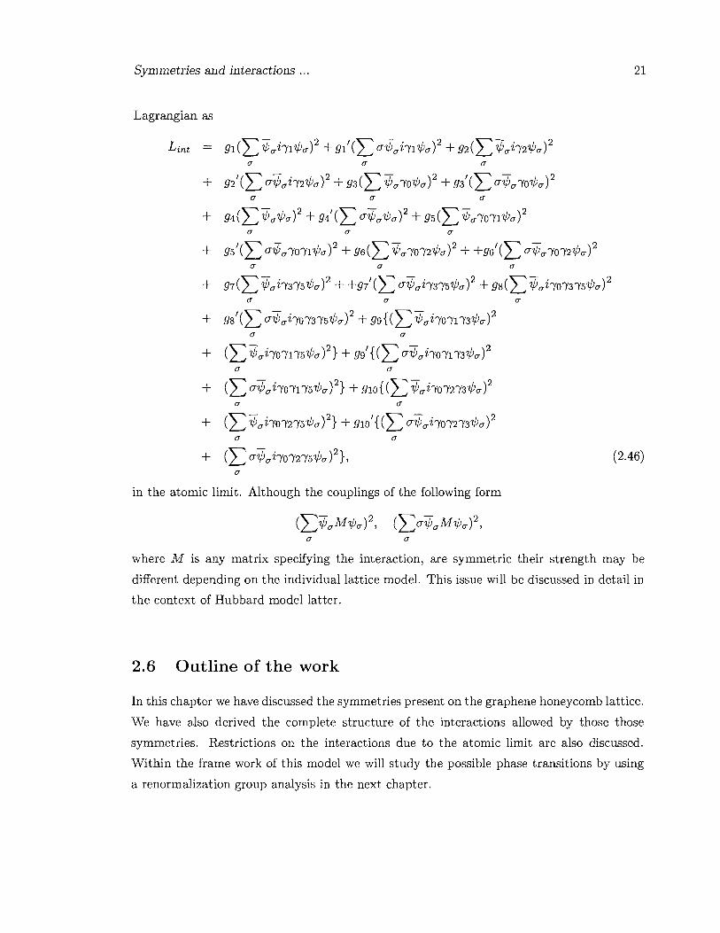
Lagrangian as

in the atomic limit. Although the couplings of the following form

17 17

21

(2.46)

where M is any matrix specifying the interaction, are symmetric their strength may be

different depending on the individual lattice model. This issue will be discussed in detail in

the context of Hubbard model latter.

2.6 Outline of the work

In this chapter we have discussed the symmetries present on the graphene honeycomb lattice.

We have also derived the complete structure of the interactions allowed by those those

symmetries. Restrictions on the interactions due to the atomic limit are also discussed.

Within the frame work of this model we will study the possible phase transitions by using

a renormalization group analysis in the next chapter.

Chapter 3

Renormalization and phase

transition

In our earlier discussions we developed the interacting theory of electrons on graphene's

honeycomb lattice that is consistent with discrete lattice symmetries. There we considered

only short ranged four-fermion interactions. From that calculation it was determined that

the theory contains 16 interactions for spinless electrons and this number gets double when

we incorporate the spin of the electrons into the theory. The number of allowed interactions

reduces to 10 once we impose the atomic limit on the spinless interactions. Constructing

the interacting theory of electrons on the honeycomb lattice it is necessary to study the

phase transitions to gapped insulating states within this model. This issue will be examined

in the following discussion. Therefore we calculate the renormalization group (RG) flows

of various couplings and present a detailed analysis on the various phase transitions from

the semimetallic ground state. Our calculations show that there exist continuous phase

transitions to charge-density-wave and anti-ferromagnetic gapped insulating ground states

with a staggered pattern in either charge or spin respectively for large enough couplings.

The transitions into these gapped insulating states generate a mass in the spectrum of the

electrons. This mechanism of generating mass through dynamical symmetry breaking is

similar to the Higg's mechanism in particle physics. Moreover we study the universality

class of those continuous quantum phase transitions and found them to be in the Gross

Neveu universality class within and also beyond the mean-field approximation. Finally, for

the Hubbard model it is shown that these two quantum critical phase transitions can be

22

Renormalization and phase transition 23

achieved by tuning repulsive Hubbard onsite interactions and nearest neighbor Coulomb

interactions to sufficiently large values. Considering the RG flows beyond the mean-field

approximation it is found that corrections to the sub-leading order in I/N provide the

semimetal state an additional protection against interactions.

3.1 Wilson's one loop renormalization

Let us now compute the flow of the couplings applying Wilson's renormalization procedure.

The usual power counting arguments imply that all short-ranged interactions are irrelevant

at the Gaussian fixed point. To gain some control over the RG flow we first deform the

Lagrangian by including N flavors of Dirac field. Therefore,

N

ww---->~WjWj.j=i

and the couplings are redefined as gi----> 2gdN [17].

(3.1)

In the Wilsonian renormalization procedure, the fast modes are confined within the

momentum shell A < k < A/b, where b(» 1) is the renormalization parameter, whereas

the slow modes correspond to momenta k < A/b. Thereafter integrating out the fast modes

A < k < A/b and over the Matsubara frequencies -00 < W n < 00 [18], we get the flow of

the different couplings at zero temperature to the sub-leading order in I/N expansion as

1 2 2 1gl - (2 - -)g] - -(g7g2 - g5g4) + -(-g2 - g3 + g4 + g5 - g6

N N N1

gs + g7 )gl + N (g3g7 - g4gS),

1 2 2 1g2 - (2 - -)g2 - -(g7g1 - g6g4) + -(-gl - g3 + g4 - g5 + g6

N N N1

gs + g7)g2 + N(g3g7 - g4gS) ,

1g3 - N (g4g5 + g4g6 + g7g1 + g7g2) ,

(3.2)

(3.3)

(3.4)


{394 =2 2 2

g4 - (4 - - )g4 - -(g3 - gl - g2 - gs - g6 + g7 + gS)g4N N

1- N (-2gSg1 - 2g6g2 + g3gs + g3g6 + glg3 + g2g3 + gSgl + gSg2)

4N (g9glO - g4g9 - g4glO), (3.5)

{395 =1 2 2 1

gs - (2 - - )gS + -(g7g6 - glg4) + -(-g6 - g7 - gl + g2 + g3N N N

1 1 2 2g4 + gs)gs - N (gSg7 + g4g3) - N (gg + glO )

2N (g9glO + gsgg + gsglO), (3.6)

{396 =1 2 2 1

g6 - (2 - - )g6 + -(g7gS - g2g4) + -(-gS - g7 + gl - g2 + g3N N N

1 1 2 2g4 + gS)g6 - N (gSg7 + g4g3) - N (gg + glO )

2(3.7)N (g9glO + g6g9 + g6glO) ,

{397 =2 2 2

g7 - (4 - - )g7 + -(g3 - gl - g2 - gs - g6 + g4 + gS)g7N N

1 2(3.8)N (-2gSg6 + gsgs + gSg6) + N (g9glO - 2g7g9 - g7glO),

{398 =1 2 2 2 (3.9)gs - N (g7gS + g7g6 - g4g1 - g4g2) + N (gg + glO ),

{399 = 2 1 2 gg ( )- gg - 2gg - - gg - - g3 + g4 - gs - g6 - g7 - gs + glON N

1 (3.10)+ N (glglO + gggs + g9g6 - g7glO + gSglO + g6glO) ,

{391O = 2 1 2 glO ( )glO - 2glO - - glO - - g3 + g4 - gs - g6 - g7 - gs + ggN N

1 (3.11)+ N (g2g9 + gggs + g9g6 - g7gg + gsgg + g6g9) ,

where {39i = d~~ib and the couplings are rescaled as giAj7f-gi. Since the model with N = 00

is exactly solvable by saddle-point methods, the leading order {3- functions may also be un

derstood as guaranteeing that the solution is cut-off independent. It is also noticed that the

renormalization with couplings gi, i = 1, ... ,8 does not generate any new couplings in a one

loop calculation. It is also noticed that the interacting Lagrangian Lint described by these

8 couplings is closed under renormalization in any order in a perturbative expansion. On

the other hand, once we incorporate gg and glO, which correspond to inter-valley scattering

Lint in the 'atomic limit' is no longer closed under renormalization. In fact the one loop

renormalization generates new terms like (1{;ir3'l/J)2, (1{;irs'l/J)2, (1{;,Or3 'l/J)2

, (1{;ror3'l/J)2. In the


large N approximation ,8-functions for different couplings do not mix as expected at the

mean-field level, but the mixing occurs when corrections of the order l/N are included. No

tice also that 9i2 term is absent in the ,8-function for the coupling 9j, where i -I j [16] and

the coefficient of 9i2 in the ,8-function for 9i vanishes for N = 1/2 [19], [20] for i, j = 1, ... ,8.

Moreover, the leading order contribution for 94 and 97 is maximal. A detailed discussion on

this issue is presented in Appendix C.

3.2 Phase transitions

Different phase transitions and also the order of that transition on the honeycomb lattice can

be determined by studying the stability of the fixed points exhibited by the flow equations.

Let us consider the mean field flow equations first. This will provide both motivation and

a guide to study the flow equations beyond the mean-field approximation. The mean-field

flow equation is obtained by setting N = (Xl in the above flow equations. Therefore the

mean-field flow equations are

(3.12)

for i = 1,2,5,6,9,10,

(3.13)

for i = 4, 7 and

(3.14)

for i = 3,8. Therefore from the mean-field analysis it is found that the fixed point at

94 = -1/4; 91 = 92 = 93 = 95 = 96 = 97 = 98 = 0 is indeed a critical point, i.e. the stability

matrix M defined as Alij = a:~i, has only one unstable direction around this point. This

critical point corresponds to a continuous quantum phase transition to the charge density

wave phase from the semimetal ground state. This critical point is found to be in the Gross

Neveu universality class [21]. Besides the charge-density-wave quantum critical point there

is another critical point at 97 = -1/4;91 = 92 = 93 = 94 = 95 = 96 = 98 = 0 that also

corresponds to a continuous phase transition. The order parameter in this insulating phase,

(;j)iry3/5VJ) , spontaneously breaks the time reversal symmetry [22]. Recently, the existence

of this phase was also predicted for strong enough next nearest-neighbor Coulomb repulsion

[23]. Other critical points corresponding to the couplings 9i, i = 1,2,5,6,9,10 are found

to be at larger couplings. Therefore any phase transition corresponding to these critical


points is prevented by the gap in either of these two channels. On the other hand the gl

and g2 couplings corresponds to the effective (2 + 1)-dimensional Thirring model for spinors

[25], [24]. It is equally interesting to study the characteristics of this phase transition beyond

mean field calculation when N = 00, in particular N = 2.

A

U-line

g.Ja

'.'.'.".".'.

'" '.'....... ,~

....... G..... ~

(-1/4,0)

,'"

(0,0)

J")

B C-.J '", (0.-1/4)

(-1/4.-1/4),~

gc,

Figure 3.1: Mean field (N = (0) flow diagram shows the quantum critical points at C, A. Gand B are the Gaussian and bi-critical fixed point. The U- line in this diagram is the lineof initial condition V = 0 in Hubbard model.

Besides the fully attractive Gaussian fixed point at gi = 0, ,8-functions in Eqs. (3.2)

(3.11) exhibit a critical point at g4 = -1/3; gl = g2 = g3 = gs = g6 = g7 = gs = 0 = gg = glO

for N = 2. This critical point (CP) corresponds to a continuous phase transition from a

semimetallic phase to a charge density wave (CDW) with a staggered pattern in charge. This

state is characterized by the order parameter C = (1[J'IjJ) (-; 0). The CDW quantum critical

point (QCP) exists at the mean-field level and also survives when sub-leading corrections

in 1/N are included. Besides the CDW QCP the fixed point at g7 = -1/3, gl = g2 =

g3 = g4 = gs = g6 = gs = gg = glO = 0 also survives as a critical point. On the other

hand the critical points corresponding to gs, g6, gg, glO are no longer critical point once we

include the corrections to the sub-leading order in 1/N. The fixed points corresponding to

gi = -2/3,gj = g3 = g4 = gs = g6 = g7 = gs = gg = glO = 0, where i,j = 1,2 but i -; j are

critical points too. Their physical significance is somewhat unclear at the moment.

We now introduce the spin degrees of freedom of the electrons to extend our discussion

on various possible phase transitions to different broken symmetry phases in spin and charge.

Renormalization and phase transition

·····..U-Line.......

ga

B

(-1/2,-1/2)

(0.0)

(0,-1/3)

~---,c

27

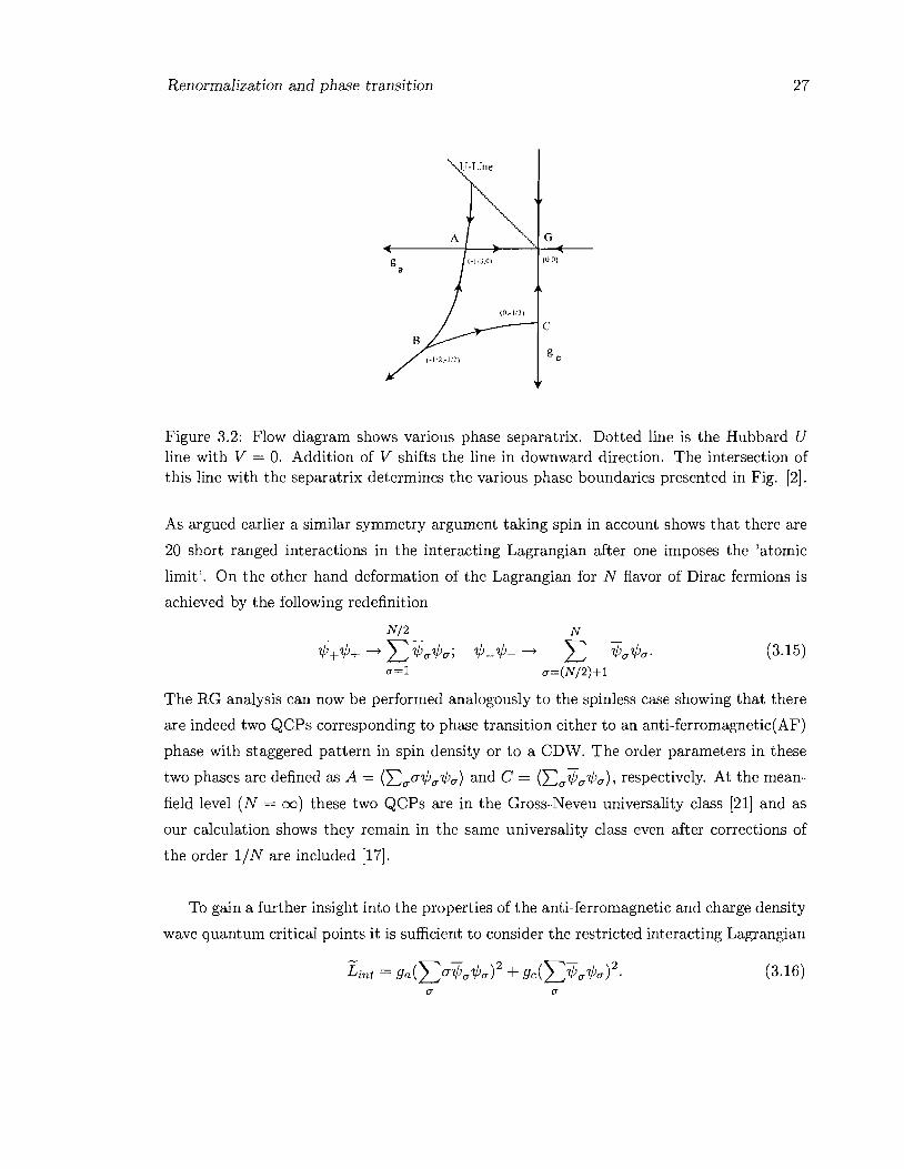
Figure 3.2: Flow diagram shows various phase separatrix. Dotted line is the Hubbard Uline with V = O. Addition of V shifts the line in downward direction. The intersection ofthis line with the separatrix determines the various phase boundaries presented in Fig. [2].

As argued earlier a similar symmetry argument taking spin in account shows that there are

20 short ranged interactions in the interacting Lagrangian after one imposes the 'atomic

limit'. On the other hand deformation of the Lagrangian for N flavor of Dirac fermions is

achieved by the following redefinition

N/2

'l/J+'l/J+ -;~ 1[;a'l/Ja;a=l

N

'l/J-'l/J- -; ~ 'l/Ja'l/Ja.a=(N/2)+1

(3.15)

The RG analysis can now be performed analogously to the spinless case showing that there

are indeed two QCPs corresponding to phase transition either to an anti-ferromagnetic(AF)

phase with staggered pattern in spin density or to a CDW. The order parameters in these

two phases are defined as A = (l:.aO"1[;a'l/Ja) and C = (l:.a1[;a'l/Ja), respectively. At the mean

field level (N = 00) these two QCPs are in the Gross-Neveu universality class [21] and as

our calculation shows they remain in the same universality class even after corrections of

the order liN are included [17].

To gain a further insight into the properties of the anti-ferromagnetic and charge density

wave quantum critical points it is sufficient to consider the restricted interacting Lagrangian

(3.16)a a


(3.17)

This only includes coupling in the anti-ferromagnetic and charge density wave channels de

noted by ga and gc respectively since these are the two QCPs (CDW and AF) exhibited by

Lint. Thus all the other couplings in Lint are irrelevant for further discussion and therefore

set to zero. In the (ga, gc) attractive plane, the QCPs corresponding to the transition from

semimetal to anti-ferromagnet(A) and charge density wave(C) are at (-1/3,0) and (0, -1/3)

respectively, beside the Gaussian fixed point(G) at (0,0) as depicted in the flow diagram.

There is also a bi-critical(B) fixed point at (-1/2, -1/2), which directs the flow towards

either the anti-ferromagnetic or charge density wave QCP. The sub-leading corrections of

the order 1/N in the beta-functions affect the flow of the couplings, resulting in the shift of

the fixed points towards the stronger coupling regime in comparison to the mean-field coun

terpart. Therefore the 1/N corrections lead to the stabilization of the semimetallic ground

state. We further notice that the sign change of the block of the matrix /0 acting on the

lower component of the spinoI' W, /0 = h&xJ"z-';(jz@(jz, together with the exchange of cou

plings ga~gc leaves Lint invariant and thus the charge-density wave and anti-ferromagnetic

critical points appear symmetrically in the (ga, gc) attractive plane. The symmetric appear

ance of these two critical points can also be argued by considering the characteristics of the

order parameters in these two phases. It is because of the preferential axis of spin, both the

charge-density wave and anti-ferromagnetic order parameter breaks the Ising like symmetry.

Hence these two quantum critical point belongs to the same universality class, Gross-Neveu

in this case.

3.3 Extended Hubbard model

Let us now consider a specific lattice model that will allow us to achieve different phase

transitions mentioned earlier by tuning some interactions already present on the lattice. The

analysis is based on a useful decomposition of Hubbard's on-site interaction on a bipartite

lattice into a sum of squares of average and staggered densities, and average and staggered

magnetizations. The Hubbard model is defined by the Hamiltonian HI, where

" _[u e2(1-8i Y )] _

HI = 0 na(X) -8i Y + _:.. nal(Y),_ ~ 2, 47rIX - YI

X,Y,o-,o-'

where the first term represent on-site repulsive interaction and the second term corresponds

to the Coulomb interaction. Hereafter we will decompose the Coulomb interaction into two


(3.18)

(3.20)

parts consisting of the nearest-neighbor repulsive Coulomb interaction denoted by V and

its long ranged tail. Even though the long ranged part of the Coulomb interaction can be

represented by a massless scalar gauge field, its main effect on the lattice scale is to provide

the repulsion between nearest-neighbors. Thus for our purposes here, consider only the

nearest-neighbor part of the Coulomb interaction. Such a decomposition of the interaction

into a short ranged and long ranged part is exact for an infinitely long-ranged one, but this

is only an approximation for the Coulomb interaction.

Generalizing the Hamman's decomposition, the first term in HI can also be written

exactly as

~ L::x [(n(A) + n(A + b))2 + (n(A) - n(A + b))2]

[(m(A) + m(A + b))2 + (m(A) - m(A + b))2],

where n(A), m(A) = u~(A)u+(A) ±u~(A)u_(A), are the particle number and the magneti

zation at the site A. Variables at the second sublattice (B) are analogously defined in terms

of vcr(13). Therefore the first term in the decomposition corresponds to the average density

on sub-lattices A and B and the second term to the difference on electron number in those

two sublattices, the third term to the average magnetization and the fourth term to the

staggered magnetization. On the other hand, the short ranged part of Coulomb interaction,

with strength V (b) can be cast in the following form

~ 2::= n(X)V(X - Y)n(Y) (3.19)x#f

= V~b) 2::= {[n(A) + n(A+ b)f - [n(A) - n(A + b)f}.X

Hence the first term of the nearest-neighbor Coulomb interaction is just the density-density

interaction and the second term is the negative interaction in the CDW channel. Thus the

strength of the interaction in CDW channel is softened by the nearest-neighbor Coulomb

interaction.

Hereafter we cast the problem in the continuum limit suitable in the low energy regime.

Defining the two slow components of fields as

12 ~ 1 if'k ~ ~rcr' (X,T) = ~ ~ -(2)2 et ,xrcr(k,T),Ik±KI<A 7f


with r = u, v, the Dirac field becomes

30

(3.21)

where 1,2 are the Dirac point indices. Therefore in terms of Dirac fields the average density,

staggered density, average magnetization and staggered magnetization read as

respectively. Noting that

and


in 'valley representation', we write down the Hubbard U-model in continuum limit as

- -+ gfC5:J (1)(YTO'l/J) 2

- g; (L (1)(YTOT1'YS'l/J)2 - g; (L U'l/J(YTOT1'Y3'l/J)2(y (y (y

- -+ gc(L1)(y'l/J? - ~C(L1)(YT1'YS'l/J)2 - ~C(L'l/J(YT1'Y3'l/J)2

(y (y (y- -

+ ga(L (1)(Y'l/J)2 - g; (L (1)(YT1'YS'l/J? - g; (L (1)(YT1'Y3'l/Jf(y (y (y

31

(3.22)

Hence in the Hubbard U-model gd = -2§d - e2/4K = (U + V)a2/8, gc = -29c = (U

V)a2/8,9f = ga = -291 = -2fia = -Ua2 /8, where the d and c couplings correspond to

the first (average density) and the second (staggered density), whereas f and a couplings

represent the third (magnetization) and the fourth (staggered magnetization) terms in HI.

The short ranged Coulomb interaction is represented by the following: (i) the intra-unit-cell,

nearest neighbor repulsion V = e2 y'3/a1r and the 2K Fourier component e2/2K. Therefore

the Hubbard model in the continuum limit dissolves into 12 couplings and all these couplings

are allowed by the symmetry present on lattice. Moreover the mean-field renormalization

calculation shows that the short ranged interactions renormalize as

(3gx = -gx - Cxgx2,

(3 - 2- 2g; = -gx + gx ,

(3.23)

(3.24)

where Cc,a = 4 and Cd,! = 0, where the couplings renormalize as gxA/1r~gx. Therefore the

fh couplings require larger interactions to open the gap in comparison to that for gx. Hence

existing gaps for finite gc,ga will prevent other gaps from opening. Therefore we can drop

all the fh for any further discussion. Therefore the semimetal-anti-ferromagnet transition is

continuous at the N = 2 Gross-Neveu critical point at which

(3.25)

with the fermion's anomalous dimension 'fN1 = [2/31r2 N] + O(1/N2) [26]'[27]. The order

parameter correlation function at the critical point also decays as

(3.26)


1.2

v0.8

04

o 0.2 04 u 0.6

Figure 3.3: The large N(blue) and N = 2(red) phase diagram for graphEme. This clearlyindicates that the semimettalic ground state is stabilized beyond mean-field. Here theaxis are in units of 8/0.2 The critical value of the Hubbard onsite repulsive interaction isUc = 0.25 for N = 00 and 0.3 for N = 2. On the other hand, the critical value of nearestneighbor Coulomb interaction for direct transition to the CD'V phase is Vc = Uc for N = 00,

but for N = 2 it is 0.33.

where T) is the standard anomalous dimension, and T) = 1 - 16/(371'2N) + 0(1/N 2). The cor

relation length diverges at the critical point with the exponent v = 1+8/(371'2N)+0(1/N 2).

The critical exponents are even calculated to the order 1/N 2 [26],[27], as well as determined

via exact renormalization group calculations [19],[20], Monte Carlo simulations, and the E

expansion, [28],129]. In summary, for N = 2, one finds 17\jJ = 0.038±0.006, v = 0.97±0.07

and 17 = 0.770±0.0016 [19][20].

Even though the long ranged nature of the Coulomb interaction is found to be marginally

irrelevant to the first order in 1/N [30]'[31],{32J as

de22

(Je = dlnb = (z - l)e ,

where z is the dynamical critical exponent found to be

(3.27)

(3.28)

similar to the bosonic case, it leaves its imprint on the bare value of the coupling gc. For a

sufficiently large value of the nearest-neighbor repulsion V, when the line of initial condition


i.e. ga = -gc for V = 0 reaches the left of the critical point C, a semimetal- charge density

wave transition occurs. This gives an alternative mechanism to that of Ref. [33],[34] for

charge density wave formation. On the other hand for a sufficiently large V when the line

of initial condition comes to the left of the bi-critical point B, a direct transition between

gapped insulating anti-ferromagnet and charge density wave state happens. This transition

is discontinuous. The phase diagram depicted in Fig[3.3] both for N = 00 and N = 2 shows

that the semimetallic state is stabilized beyond the mean-field approximation.

Chapter 4

Conelusions

Within the framework of the tight-binding model it is found that at half-filling the valence

and conduction bands touch each other at the Dirac points, located at the corners of the

Brillouin zone and electron behaves like massless pseudo-relativistic Dirac fermion, where

the Fermi velocity (rv 106 m/s) plays the role of the velocity of light. It also turns out that

out of six such Dirac points only two are non-equivalent. Therefore at energy scales much

lower than the bandwidth only electrons near these points carry dynamical importance.

Hence we construct the interacting theory of electrons on the honeycomb lattice in terms of

Dirac fields by considering the four-fermionic short ranged interactions.

Discrete symmetries of the honeycomb lattice allow us to restrict the number of short

ranged interactions in the continuum limit. Interchange of the labeling of two triangular

sub-lattices of the honeycomb lattice presents a discrete symmetry of the lattice daubed as

'mirror symmetry'. Another discrete symmetry comes from relabeling of two non-equivalent

Dirac points. We recognize this symmetry as the time-reversal symmetry of the problem.

We argued here that the labeling of the two sub-lattices and the Dirac points is completely

arbitrary and therefore the theory should remain invariant under relabeling.

Further restriction on the interactions is achieved by considering momentum conserva

tion at the two Dirac points. Altogether these symmetries restrict the interacting theory

to 16 couplings when we suppress the spin degrees of freedom of the electrons. Here we

also considered the parity symmetry on the lattice and found an explicit representation in

the continuum limit. It turns out that all the interactions are invariant under the mirror,

34

Conclusions 35

time reversal, and parity symmetries combined. The number of interactions defining the

interacting Lagrangian is further reduced by imposing the atomic limit. In the atomic limit

the interacting Lagrangian is defined by 10 couplings for spinless electrons. When we incor

porate the spin degrees of freedom into our theory the number of interactions allowed by

the symmetry and atomic limit both gets double. This can be achieved by generalizing the

discussion on symmetry for spinless electron after including the spin degrees of freedom.

Furthermore, analyzing the renormalization group flows, derived by using Wilson's one

loop method with the interacting model in the atomic limit, we found that there exists a

continuous phase transition to a charge density wave phase from the semimetallic ground

state for spinless electrons. Considering the spin of the electrons we found that there ex

ists an additional continuous phase transition to the anti-ferromagnetic phase. These two

quantum phase transitions exist at the mean-field level and also survive when we consider

sub-leading corrections in liN. These two quantum phase transitions are found to be in

the Gross- Neveu universality class for large N and remains in the same universality class

for finite number of fermionic species on the lattice. On the other hand, corrections to

the sub-leading order in liN provide an extra protection to the semi-metallic ground state

against interactions by slowing down the flow of the couplings towards the critical points. It

is also argued that the interactions corresponding to intra-valley scattering are closed under

renormalization to any order in perturbation theory. On the other hand, once we incorpo

rate the interactions corresponding to inter-valley scattering the model in the atomic limit

is no longer closed under renormalization.

Beside the charge-density wave quantum critical point the spinless interacting model

also exhibits another critical point that corresponds to a continuous phase transition into

a gapped insulating phase. The order parameter in this phase spontaneously breaks time

reversal symmetry.

Finally we consider the extended Hubbard model with both an on-site (U) and a nearest

neighbor (V) Coulomb repulsive potential. Neglecting the long ranged part of the Coulomb

interaction we found that it is defined by 12 short ranged couplings. Parameterizing the

couplings with U and V we thereafter extract the phase diagram showing the semimetal

charge density wave and anti-ferromagnet transition for sufficiently large U and V. In that

Conclusions 36

phase diagram we also found a discontinuous transition between the charge density wave

and anti-ferromagnet for large enough V.

Appendix A

Momentum shell integration in one

loop Wilsonian renormalization

Let us consider the model with only two couplings

(A.I)

where M 1 and M 2 are some Dirac matrices. To calculate the {3- function to leading order

in liN we have to compute the following integral

(A.2)

where f-L, 1/ = 0, l, 2 and i, j = I, 2 at one loop level. Because of the cyclic property of the

trace we need i = j, otherwise the trace vanishes. Therefore to leading order in liN the

two different couplings do not mix and we found

for M = 1,'3'5,

AR1 = -lnb,

7f(A.3)

AR 1 = ±-In b, (A.4)

27f

for M = ,1, ,2, ,0,1, ,0,2 (upper sign), M = ,113, ,115, ,0,113, '0,115 (lower sign) and

(A.5)

for M = ,0, ,0,315. On the other hand we will encounter the following integral

(A.6)

37

Nlomentum shell integration ... 38

in calculating the (3 functions to sub-leading order in liN. This integral may give a non

trivial result depending Ali and M j explicitly. In a diagrammatic calculation this contri

bution is generated by the particle-hole diagram. On the other hand if we consider the

particle-particle diagram it will leave us with the following integral

lA kdk 100dwR3- - -

Alb 21T" -00 21T"

kJi-( -kv )

(k2 + w2)2'(A.7)

The minus sign in front of the momentum kv comes from momentum conservation in the

loop. For i = j, it is trivial to check that R2 and R3 cancel each other but these two may

add for i of j and generate new couplings. For example if we consider M l = I and M2 = ')'0

then the contributions from two such diagrams will add and generate the following two new

couplings

We can generalize these arguments after including the spin degree of freedom.

(1)

(2)

Figure A.I: Particle-hole and particle-particle diagrams at the one loop level without spindegrees of freedom may generate new coupling to sub-leading order in liN depending onthe integrals R2 and R3.

Appendix B

Flow equations

In this discussion we present the renormalization flow of the couplings defined the interacting

Lagrangian (Lint) including the spin degree of freedom of electron. In Chapter 2, we found

that when we incorporate the spin of the electrons, Lint is defined in terms of 16 coupling

constants in the atomic limit. Even though in the mean-field approximation all the couplings

are decoupled from each other, mixing may appear non-trivially at sub-leading order in liN.

On the other hand, when we take the spin degrees of freedom into account an additional

complication arises since all the couplings become two-fold degenerate in bilinear space and it

is thus impossible to determine after the fast mode and frequency integration which coupling

gets renormalized if we consider the mixing of couplings 9i and 9/, for i = 1, ... ,8. Therefore

special care is required. Here we present the solution of this problem by considering the

mixing of 94 and 9i couplings as follows

94(L cy1[;a1/;a)2 +94'(L 1[;a1/;a)2a=± a=±

(B.1)

where, 9+ = 94 + 94' and 9- = 94 - 9i. The flow equations in terms of these two couplings

read

{3g+ = -9+- (2 - ~) 9+ 2 ~ 29_ 2, (B.2)

{3g_ = -9-- (4 - ~)9+9-· (B.3)

This procedure can easily be extended for other such pairs of couplings. This complication

does not appear if we consider the mixing of two couplings with different order parameters.

39

Flow equations 40

In the Wilsonian one loop calculation the flow equation of different couplings in Lint is

given by

(B.8)

(B.9)

2 2 2 , , ,- 94 - (4 - N)94 + N94( -91 - 92 + 93 - 95 - 96 + 97 + 98 - 91 - 92 + 93

, , , , ') 2 ( , , ") I (+ 94 - 95 - 96 + 97 + 98 + N 9195 + 9195 + 9296 + 9296 - N 9395 + 9396

+ 93'95' + 93'96' + 9391 + 9392 + 93'91' + 93'92' + 9891 + 98'9/ + 9892 + 98'92')

(B.IO)

Flow equations 41

'( 2) '2 2 , ( , ,(394' - 94 - 4 - N 94 + N 94 -91 - 92 + 93 + 94 - 9s - 96 + 97 + 9s - 91 - 92

, , , , ') 2 ( " ") 1 (' ,+ 93 - 9s - 96 + 97 + 9s + N 919s + 91 9s + 9296 + 92 96 - N 939s + 9396

, , , , , , " ")+ 93 9s + 93 96 + 9391 + 9392 + 93 91 + 93 92 + 9s91 + 9s 91 + 9s92 + 9s 92

(B.ll)

(B.12)

, 1) '2 1 '(9s - (2 - N 95 + N95 -91 + 92 + 93 - 94 + 95 - 96 - 97 + 9s

, , , , , , ') 1 ( , ,91 + 92 + 93 - 94 - 96 - 97 + 9s - N 9394 + 9394 + 979s

") 2 ( , , , ')+ 979s + N 9796 + 9796 - 9194 - 91 94 (B.13)

(1 2 1 ,

(3g6 = - 96 - 2 - N )96 + N96(91 - 92 + 93 - 94 - 95 - 97 + 9s + 91

, , , , , , ') 1 ( , , , ')92 + 93 - 94 - 95 + 96 - 97 + 9s - N 9394 + 9394 + 979s + 97 9s

2 ( , , , ') (B 14)+ N 9795 + 9795 - 9294 - 92 94 .

'( 1) '2 1 '(96 - 2 - N 96 + N96 91 - 92 + 93 - 94 - 95 + 96 - 97 + 9s

, , , , , ') 1 ( , "+ 91 - 92 + 93 - 94 - 97 + 9s - N 93 94 + 9394 + 97 9s

') 2 ( , , , ')+ 979s + N 9795 + 97 95 - 92 94 - 9294 (B.15)

(B.16)

Flow equations 42

1 ( 2 /2 2 1 IIf397' = 97 - 4 - N)97 + N97 (-91 - 92 + 93 + 94 - 95 - 96 + 97 + 98 - 91 - 92

1 1 1 1 I) I ( 1 1 1 I)+ 93 + 94 - 95 - 96 + 98 - N 9895 + 98 95 + 98 96 + 9896

2 1 1 (N (9695 + 9596 ) B.I7)

f3 I ( 1 1 1 1 1 1 1 I)98 = -98 - N 9795 + 97 95 + 9796 + 97 96 - 9491 - 94 91 - 9492 - 94 92 ,

(B.I8)

f3 1 I ( 1 1 1 1 1 1 1 I)98' = -98 - N 97 95 + 9795 + 97 96 + 9796 - 9491 - 9491 - 94 92 - 9492 ,

(B.I9)

at zero temperature. Here we considered couplings corresponding to intra-valley scattering.

Notice that even though we started with a model where only 93 and 94 are finite for

spinless electrons, the subleading order corrections in liN generate all the other possible

couplings allowed by symmetry. In the diagrammatic renormalization calculation the one

loop particle-particle and some particle-hole diagrams generate new couplings when the sub

leading order corrections in liN are included.

Flow equations

(1)

(3)

(5)

(2)

(4)

(6)

43

Figure B.l: Feynman diagrams contributing to the leading order and the sub-leading orderin liNin renormalization of couplings in the one-loop level. In the diagrams a solid linestands for the field with spin-up component and the dashed line corresponds to that withspin-down component. Diagram (1) contributes in both leading and sub-leading order,whereas the diagram (3) contributes only to the sub-leading order renormalization of the 9+coupling. On the other hand diagram (2) and diagram (4) renormalize the 9_ coupling bothin leading and sub-leading order but only sub-leading order in liN respectively. A replicaof the second diagram, where the propagators are built out of the spin-down fields alsorenormalizes the 9_ coupling to both leading and sub-leading order in liN. Diagrams (5)and (6) renormalize 9_ to the sub-leading order in liN. However these two contributionscancel each other if we consider the mixing of two couplings degenerate in bilinear spacewhereas they add and may generate new couplings if we consider couplings having differentbilinear.

Appendix C

Susceptibilities of Dirac fermions

in (2+1)-dimensions

In this appendix we answer the question as to which bilinear has the largest susceptibility

in (2 + 1)- dimensions. To answer this question let us consider the free Lagrangian

with a bilinear 'order parameter' "ijjM'IjJ

L = "ijj[N + ij"ijjM'IjJ,

where i, j are source fields. Integrating out the fermions gives

where X is the required susceptibility given by

Here our main concern is to find XO = X(q = 0), given by

(C.1)

(C.2)

(C.3)

(C.4)

(C.5)

For D = 3 one finds

(C.6)

44

Susceptibilities of Dirac fermions ...

Hence our task is to find the M which gives the largest trace.

Let us now introduce a basis r 0: E

{I 10 II 12 13

10111213 = 15}.

All the elements in this basis satisfy the following properties

Expanding M in this basis one gets

T = L CaCb Tr btlraltLrb) ,tL,a,b

45

(C.7)

(C.8)

where, T = TrbtLM'tLM) and M = l:aCara. Using the fact that the elements in r Q either

commute or anti-commute with ItL one can decompose T as follows

T = LLCb {L' CaTr(rarb) - L"CaTr(rarb)},tL b a a

(C.g)

since Ii = I for all p. In the above expression l:a' runs over ra which commutes with ItL

and l:a" runs over r a which anti-commute with ItL. Since

one gets

T = 4L (L' Ca2- L"Ca2) .tL a a

Therefore we get the bounds on T as

-4 x 3 < T ~4 x 3,

(C.IO)

(C.lI)

(C.12)

Susceptibilities of Dirac fermions ...

assuming :LaCa2 = 1. Thus the trace optimized in two cases, either

{NI, rll} = 0,

for all f-L, implying M = r3, r5, or

46

(C.13)

(C.14)

for all f-L, implying M = I, ir3'Y5 . Hence from these solutions one immediately finds that

the susceptibility of Dirac fermions in (2 + I)-dimensions is maximized for M = I, ir3, ir5,and ir3r5, whereas it is minimum for M = r3, r5, and r3r5. Therefore the maximal suscep

tibility corresponds to the opening of the relativistic mass gap that either breaks the chiral

symmetry (ro, iror3, irOr5) or doesn't break the chiral symmetry (iror3'Y5).

On the other hand the susceptibility of the Dirac fermions is largest only for M

rO, irOr5 for D = 3 + 1.

Bibliography

[1] KS. Novoselov, A.K Geim, S.V. Morozov, D. Jiang, Y. Zhang, S.V. Dubonos, LV.

Gregorieva and A.A. Fishov, Science 306, 666 (2004).

[2] A.K Geim and A.H. McDonald, Physics Today 60, 35 (2007).

[3] P.R. Wallace, Phys. Rev. 71 622 (1947).

[4] A.H. Castro Neto, F. Guinea, N.M.R. Peres, KS. Novoselov, and A.K Geim,

cond-mat/ 0709.116 vI (2007).

[5] A.H. Castro Neto, F. Guinea, and N.M.R. Peres, Physics World 19, 33 (2006).

[6] M.L Katsnelson, and KS. Novoselov, Sol. Stat. Comm. 143, 3 (2007).

[7] M.L Katsnelson, Eur. J. Phys. B 51, 157 (2006).

[8] V.P. Gusynin, and S.G. Sharapov, Phys. Rev. Lett. 95, 146801 (2005).

[9] N.M.R. Peres, F. Guinea, A.H. Castro Neto, Phys. Rev. B 73, 125411 (2006).

[10] KS. Novoselov, A.K Geim, S.V. Morozov, D. Jiang, M.L Katsnelson, Y. Zhang,

S.V. Dubonos, LV. Gregorieva, and A.A. Firsov, Nature 438, 197 (2005).

[11] Y. Zhang, Y.W. Tan, H.L. Stormer, and P. Kim, Nature 438, 201 (2005).

[12] M. Stone, Quantum Hall Effect (World Scientific, Singapore), 1992.

[13] F. Bassani, G. Pastori Parravicini, Electronic States and Optical Transitions in Solid

(Pergamon, New York, 1975).

[14] G.W. Semenoff, Phys. Rev. Lett. 53, 2449 (1984).

47

Bibliography

[15] C.Y. Hou, C. Chamon, C. Mudry, Phys. Rev. Lett. 98, 186809 (2007).

[16] K. Kaveh, I.F. Herbut, Phys. Rev. B 71, 184519 (2005).

[17] I.F. Herbut, Phys. Rev. Lett. 97, 146401 (2006).

48

[18] I.F. Herbut, A Modern Approach to Critical Phenomena (Cambridge University Press,

Cambridge, England, 2006), Chap. 8.

[19] L. Rosa, P. Vitale, and C. Wetterich, Phys. Rev. Lett. 86, 958 (2001).

[20] F. Hofting, C. Novak, and C. Wetterich, Phys. Rev. B 66, 205111 (2002).

[21] D. Gross and A. Neveu, Phys. Rev. D 10, 3235 (1974).

[22] F.D.M. Haldane, Phys. Rev. Lett. 61, 2015 (1988).

[23] S. Raghu, Xiao-Liang Qi, C. Honerkemp, and Shou-Cheng Zhang, Phys. Rev. Lett.

100, 156401 (2008).

[24] I.F. Herbut, and D.J. Lee, Phys. Rev. D 68, 104518 (2003).

[25] K.I. Kondo, Nuc!. Phys. B 450, 251 (1995).

[26] A.N. Vasil'ev, S.E. Derkachev, N.A. Kievl', and A.S. Stepanenko, Theor. Math.

Phys. (Eng!. Trans!.) 94, 127 (1993).

[27] J.A. Gracey, Int. J. Mod. Phys. A 9, 727 (1994).

[28] L. Karkkainen, L. Lacaze, P. Lacock, and B. Petersson, Nuc!. Phys. B 415, 781

(1994).

[29] L. Karkkainen, L. Lacaze, P. Lacock, and B. Petersson, Nuc!. Phys. B 438, 650(E)

(1995).

[30] J. Gonzales, F. Guinea, and M.A.H. Vozmediano, Nuc!. Phys. B 424, 595 (1994).

[31] J. Gonzales, F. Guinea, and M.A.H. Vozmediano, Phys. Rev. B 59, R2474 (1999).

[32] O. Vafek, Phys. Rev. Lett. 97, 266406 (2006).

[33] D.V. Khveshchenko, Phys. Rev. Lett. 87, 246802 (2001).

[34] D.V. Khveshchenko, H. Leal Nucl. Phys. B 687, 323 (2004).

SYMMETRIES, INTERACTIONS AND PHASE...

Documents

Transcript of SYMMETRIES, INTERACTIONS AND PHASE...