Structural Changes and Growth Regimes

Tommaso Ciarli, André Lorentz, Marco

Valente and Maria Savona

SWPS 2017-12 (June)

Guidelines for authors

Papers should be submitted to swps@sussex.ac.uk as a PDF or Word file. The first page

should include: title, abstract, keywords, and authors’ names and affiliations. The paper will

be considered for publication by an Associate Editor, who may ask two referees to provide a

light review. We aim to send referee reports within three weeks from submission. Authors

may be requested to submit a revised version of the paper with a reply to the referees’

comments to swps@sussex.ac.uk. The Editors make the final decision on the inclusion of the

paper in the series. When submitting, the authors should indicate if the paper has already

undergone peer-review (in other series, journals, or books), in which case the Editors may

decide to skip the review process. Once the paper is included in the SWPS, the authors

maintain the copyright.

Websites

UoS: www.sussex.ac.uk/spru/research/swps

SSRN: http://www.ssrn.com/link/SPRU-RES.html

IDEAS: ideas.repec.org/s/sru/ssewps.html

Research Gate: www.researchgate.net/journal/2057-6668_SPRU_Working_Paper_Series

Editors ContactTommaso Ciarli T.Ciarli@sussex.ac.uk

Daniele Rotolo D.Rotolo@sussex.ac.uk

Associate Editors Area

Karoline Rogge Energy K.Rogge@sussex.ac.uk

Paul Nightingale,

Ben Martin, &

Ohid Yaqub

Science, & Technology Policy P.Nightingale@sussex.ac.uk

B.Martin@sussex.ac.uk

O.Yaqub@sussex.ac.uk

Tommaso Ciarli Development T.Ciarli@sussex.ac.uk

Joe Tidd &

Carlos Sato

Technology Innovation Management J.Tidd@sussex.ac.uk

C.E.Y.Sato@sussex.ac.uk

Maria Savona Economics of Technological Change M.Savona@sussex.ac.uk

Andrew Stirling Transitions A.C.Stirling@sussex.ac.uk

Caitriona McLeish Civil Military Interface C.A.McLeish@sussex.ac.uk

Editorial Assistance

Martha Bloom M.Bloom@sussex.ac.uk

SPRU Working Paper Series (ISSN 2057-6668)

The SPRU Working Paper Series aims to accelerate the public availability of the research

undertaken by SPRU-associated people, and other research that is of considerable interest

within SPRU, providing access to early copies of SPRU research.

Structural Changes and Growth Regimes∗

Tommaso Ciarli † Andre Lorentz ‡ Marco Valente § Maria Savona ¶

This version: June 14, 2017First version: June 2016

Abstract

We study the relation between income distribution and growth mediated by structuralchanges on the demand and supply side. Using results from a multi-sector growth model wecompare two growth regimes which differ in three aspects: labour relations, competition, andconsumption patterns. Regime one, similar to Fordism, is assumed to be relatively less un-equal, more competitive, and with more homogeneous consumers than regime two, similarto post-Fordism. We analyse the parameters that define the two regimes to study the role ofexogenous institutional features and endogenous structural features of the economy on outputgrowth, income distribution, and their relation. We find that regime one exhibits significantlylower inequality, higher output and productivity, and lower unemployment than regime two.Both institutional and structural features explain these difference. Most prominent amongthe first group are wage differences, accompanied by capital income, and the distribution ofbonuses to top managers. The concentration of production magnifies the effect of wage dif-ferences on income distribution and output growth, suggesting the relevance of the norms ofcompetition. Among structural determinants, particularly relevant are firm organisation andthe structure of demand. The way in which final demand distributes across sectors influencescompetition and overall market concentration. Particularly relevant is the demand of the leastwealthy classes. We also show how institutional and structural determinants are tightly linked.Based on this link we conclude by discussing a number of policy implications emerging fromour model.

Keywords:Structural change; income distribution; competition; consumption behaviour;technological change

JEL: O41, L16, C63, O14

∗We thank participants at the following conferences for comments and suggestions: EURKIND (Valencia, 2016),Schumpeter Society (Montreal, 2016), SPRU50 (Sussex, 2016), and EAEPE (Manchester, 2016). We thank participantsin seminars at ECLAC, ECLAC summer school, and Curitiba for comments and suggestions. The paper has greatlybenefited from comments and suggestions from Robert Blecker, Francesco Lamperti, Carolina Pan, Gabriel Porcile,Anna Salomons, Engelbert Stockhammer, Ariel Wirkierman, an anonymous reviewer of the SPRU Working PaperSeries, and two anonymous referees of this journal. The paper has benefited from funding from the European Union’sHorizon 2020 research and innovation programme under grant agreement No. 649186 – Project ISIGrowth.

†SPRU, Science Policy Research Unit, University of Sussex, UK, T.Ciarli@sussex.ac.uk‡BETA (UMR-CNRS 7522) Universite de Strasbourg and x , France, alorentz@unistra.fr§University of L’Aquila, Italy; SPRU, University of Sussex; Ruhr-Universitaet Bochum; LEM, Sant’Anna School

for Advanced Studies, marco.valente@univaq.it¶SPRU, Science Policy Research Unit, University of Sussex, UK, M.Savona@sussex.ac.uk

1

1 Introduction

An increasing number of studies suggest that most OECD economies have changed growth regimearound the 1980’s (Freeman and Soete, 1997; Fagerberg and Verspagen, 1999; Petit, 1999; Boyer,2010). Some of the regularities that suggest a change in the growth regime across a range ofcountries are in order.

Atkinson (2015), Atkinson and Morelli (2014), and Piketty (2014), among many others, sug-gest that income inequality has been rising since the 1980’s, after a few decades of decline. Whilethere are important differences in the level of inequality among countries with different welfarestates, the pattern has been similar across OECD countries.

Such increase in inequality was accompanied by a number of related changes, also commonacross a range of OECD countries. Inequality seem to be driven by the increased share of wealthconcentrated in the 10% and the 1% of the population with the highest incomes (Alvaredo et al.,2013; Atkinson et al., 2011; Atkinson and Morelli, 2014). Since the 1970’s the increase in in-equality was preceded, and is currently accompanied, by a regular decline of labour shares (overGDP) (Karabarbounis and Neiman, 2013; Summers, 2013). Related to this, wage growth and pro-ductivity growth, once matched, started to diverge at the end of the 1970’s, with the gap betweenthe two increasing constantly (Lazonick, 2014).

Similar to what happened during other episodes of structural change, process innovation inthe manufacturing sector is increasingly labour saving: capital goods replace more and moreroutinised tasks, increasing productivity (Brynjolfsson and McAfee, 2014; Karabarbounis andNeiman, 2013). Labour economists have convincingly shown that this is followed by an increasein the number of low paid jobs, and an increase in the number of high paid jobs (Acemoglu andAutor, 2011), reducing significantly the middle class jobs. Manning (2004), Autor and Dorn(2013), and Mazzolari and Ragusa (2013) also suggest that these changes in the labour market arenot independent from changes in the composition of consumption and consumer preferences.

A large component of the increasing difference between the top 10% and the rest is the in-creased compensations of top classes of workers, with wages, bonuses, profit shares (Atkinsonet al., 2011) and stock options (Frydman and Jenter, 2010). Part of these growing differences areexplained by the routinisation of tasks, and part by the financialisation of economies and firms (La-zonick, 2014; Lazonick and Mazzucato, 2013; Stockhammer, 2012). The trend which is commonto both is the increased size of firms. The evidence shows that firm average size increases with acountry per capita income (Poschke, 2015) and market concentration (The Economist, 2016), andis correlated with wage dispersion (Mueller et al., 2015) and CEO pay rise (Frydman and Jenter,2010). OECD (2017) suggest that recent innovations have increased market concentration andthe innovation rents redistributed to shareholders and managers. And Autor et al. (2017) suggestthat the fall in labour share is related to increase in market concentration and firm size which isalso due to change in consumer behaviour, innovation, and lower rates of creative destruction. Assuggested by The Economist, “part of what is perceived as a global trend towards greater disparityin wages may actually be the result of the biggest firms employing a greater share of workers”.

In this paper we study the relation between income distribution and growth mediated by struc-tural changes on the demand and supply side. We study how the relation changes for distinctgrowth regimes (Boyer, 1988; Petit, 1999; Coriat and Dosi, 2000) characterised by endogenousdifferences in (i) labour relations – compensation, profit shares, and the elasticity of wages with re-spect to productivity and inflation; (ii) norms of competition – entry barriers and market selection;and (iii) income related norms of consumption – consumption shares and consumer preferences.We focus only on structural determinants of income inequality, and we do not consider leavingany redistributive policy.

We define two regimes. Regime one characterised by relatively more equal labour relations,more competition and lower selection, and smaller difference in consumption behaviour; and

2

regime two relatively more unequal, with relatively more protection for incumbents but higher mar-ket selection, and larger differences in consumption behaviour. Although we do not aim to repli-cate any specific historical period, one may think of regime one as a Fordist regime and regime twoas a post-Fordist regime. Instead, we compare the two regimes using results from a multi-sectormodel that associates the different regimes to different dynamics of structural changes. We thenstudy which of the three aspect that in our model define the regimes is more relevant in explainingthe relation between income distribution and growth, by means of a parametric analysis.

We find that a Fordist regime (one) exhibits significantly lower inequality, higher output andlower unemployment than a Post-Fordist regime (two). We distinguish between institutional andstructural determinants of these differences, although we also suggest that the two types of deter-minants are strongly related. Institutional determinants are used to differentiate the two regimeswith respect to labour relations, norms of competition, and norms of consumption. We find that,keeping all other features of the regimes fixed, wage differences play the most important role inincreasing inequality and limiting output growth. Returns on capital and bonuses to managersmagnify the effect of wage differences by increasing the wealth of high wage earners with respectto low wage earners. The role of the minimum wage, instead, is substantially weaker. The concen-tration of production also magnifies the negative effect of labour relations on income distributionand output growth, suggesting the relevance of the norms of competition. However, in our modelwe find two opposite effects. On the one hand concentration through entry barriers increases in-equality and reduces output growth. On the other hand, concentration via market selection reducesinequality, but has no effect on output. Finally, the norms of consumption have no significant effecton either income distribution or output.

Structural determinants, instead, are emerging properties in our model. First, in the absence ofredistributive policies, an increase in average firm size have a direct effect on increasing incomeinequality. Changes in the structure of production amplify the effect of institutional difference inwage setting. Second, the structure of the demand also plays a crucial role. Sectors that attract thelargest share of consumption of low income classes tend to be also significantly less concentratedin our model than sectors that sell mainly luxury goods. The structure of demand also influencescompetition: sectors that constitute the largest expenditure shares of the low income classes facefiercer competition, more selective consumers with respect to price, and therefore tend to exhibita low mark-up. This implies lower profits and dividends which would accrue wealthier classesincome. Third, demand plays a crucial role in explaining the differences in output between thetwo regimes. Even if regime two catches up in terms of productivity, due to the structure ofdemand the more uneven distribution curtails output growth.

Modelling and Defining Growth Regimes

The interaction between labour compensation, competition, and consumption patterns has beendiscussed by the regulation theory with reference to different varieties of capitalism (Boyer (1988),Petit (1999) and Coriat and Dosi (2000)).

We propose a model in which we interpret these three aspects as follows.Labour compensation, the wage-labour nexus. We distinguish three aspects of the wage labour

nexus. First, we model firms as hierarchical organisations (Caliendo et al., 2015), where workersare distributed in different tiers with different tasks and wages: at the bottom of the pyramid areclerks and blue-collars, at the top are the CEOs. In between, there are a number of intermediatesupervisors and managers. The number of managerial tiers depends on the organisation of labourand on the size of the firm (endogenous in our model). Small firms have less tiers than large firms,cœteris paribus. Firm size depends on consumer selection, the level of consumer demand, labourproductivity, and the entry of new competitors. Wages are differentiated across tiers, determiningincome differences between consumer classes. Together, the number of tiers and the wage dif-ferences determine the distribution of wages in the population. The larger is the wage multiplier,

3

the larger the difference between tiers. Second, workers in managerial positions receive part ofthe profits as bonuses or profit shares as part of their compensation, proportionally to their basewage. The larger is the rate of profits distributed as bonuses, the larger are the differences betweenworking classes. Third, the minimum wage is a function of unemployment, average productivity,and inflation. We peg changes in the minimum wage to changes in productivity and prices. Thelarger the elasticity of the minimum wage to productivity and inflation, the higher the distributionof value to workers, and the higher their purchasing power (level of demand).

Norms of competition. In our model competition and market concentration depend on con-sumers’ selection, firms’ differentiation with respect to price and quality, and entry barriers. Con-sumers’ selection and firm’s heterogeneity are endogenous in the model. Selection depends onthe changes in the structure of consumer classes and on their preferences; firms’ heterogeneity de-pends on firms response to price competition (investing in newer and more efficient capital goodsand changing the mark-up) and non-price competition (increasing the quality of their products).We distinguish two aspects of the norms of competition. First, the lower are entry barriers, thehigher is the probability that new firms enter in one of the consumer goods sectors and com-pete. Second, the more selective are consumers’ preferences with respect to quality and price, thestrongest the selection of firms, and the lower the number of surviving firms.

Norms of consumption. We model two aspects of changes in consumption behaviour. First,consumers in different income/working classes consume a different share of goods from each finalgood sector in the economy. We assume that less wealthy classes consume mainly basic goods andsmaller shares of luxury goods. The opposite is true for the asymptotically wealthiest class. Thefastest the change in consumption shares between consecutive classes the more heterogeneousis the demand between income classes at the extremes of the distribution. Second, we modelpreferences as the selectivity with respect to prices and quality. We assume that consumers inclasses with a lower income tend to be more selective on price and less selective on quality, withrespect to higher income consumers. These preferences change from one class to the next: thelarger is the change, the larger are the differences between classes.

The three dimensions of the growth regimes are endogenously related in our model. Firm size,which determine the organisational tiers and wage difference, depends on the level of the demandand on market concentration. The level of demand depends on the elasticity of the minimumwage to changes in prices. Market concentration depends on the norms of competition and onthe concentration of the demand. In turn, consumers demand depends on how they are distributedamong classes and on the income of each class, which depends on the organisational tiers andon the wage differences. In other words, the norms of consumption are partly endogenous to thewage-labour nexus; the norms of competition are partly endogenous to norms of consumption;and the wage-labour nexus is partly endogenous to both competitions and consumption norms.

We distinguish two growth regimes. Regime one is characterised by lower differences in com-pensation across hierarchical tiers, a lower share of profits distributed to managers as bonuses, anda higher elasticity of the minimum wage to changes in prices and productivity. In other wordsregime one assumes a lower personal and functional income inequality. In regime one, marketbarriers are lower and consumers are less selective with respect to both price and quality. Finally,consumption patterns change at a slower pace and the preferences of middle income classes arecloser to those of the lower than to the higher income classes. Such a regime is relatively closer towhat the regulation school defines the Fordist regime.

Regime two is characterised by larger differences in compensation across hierarchical tiers,a larger share of profits distributed to managers, and a lower elasticity of wages with respect tochanges in prices and productivity. Regime two assumes a higher personal and functional incomeinequality. In regime two market barriers are higher and consumers are more selective with respectto both price and quality. Finally, consumption patterns change at a faster pace and the preferencesof middle income classes are closer to those of the richer than to those of the less wealthy classes.

4

Such a regime is relatively closer to what the regulation school defines the post-Fordist regime.

Relevant Literature

To our knowledge, most growth models that discuss growth regimes focus on the long run growthand on the shifts in growth patterns, such as the unified growth theory (Galor, 2007). For exampledue to changes in birth and education household strategies (Galor and Weil, 2000; Boucekkineet al., 2002), firm growth (Desmet and Parente, 2012), or changes in technology and demand(Ciarli et al., 2012). Empirically, a number of studies investigate structural breaks in growthpatterns, particularly focusing on developing countries (Kar et al., 2013; Lamperti and Mattei,2016; Pritchett, 2000). Jones and Olken (2008) characterise the transition between regimes andfind that different countries follow common experience of growth acceleration and declines.

Napoletano et al. (2012) is one of the few papers that attempts to model regimes based oninsights from the regulation school. The authors mainly focus on the relation between income dis-tribution and firm investment behaviour (in new process technologies). Taking an evolutionary ap-proach, and focussing on how micro behaviour affect macroeconomic outcomes, they investigate“how different growth regimes emerge out of micro-interactions between heterogeneous agents”.The paper discusses two different regimes. One where employment is a consequence of increaseddemand through investment, spurred by profit inducing productivity enhancing innovation. A sec-ond one where investment is not led by profits but by demand expectations, and productivity gainsare shared between capital goods and labour. As a result, an increase in productivity also leads toincreased demand via both consumption and investment.

Our paper is similar in spirit. We model how different ways of organising microeconomicinteractions may lead to different macroeconomic outcomes. We add to the work of Napoletanoet al. (2012) by being more explicit in modelling the labour relations, the forms of competition,and the norms of consumption, and how differences in those three dimensions may be described asdifferent regimes, or different forms of capitalism. To our knowledge this is also the first paper thatinvestigates how structural changes are related to different growth regimes, and how they mediatethe relation between growth and distribution of income under different regimes.

Focusing on the relation between structural changes and growth regimes this paper contributessubstantially to the growing literature on Agent-Based macroeconomics1 and to evolutionary eco-nomic growth models2. The paper is closely related to papers that study the interaction betweenSchumpeterian and Keynesian dynamics using agent based micro foundations (Dosi et al., 2010,2015, 2013). It is also related to the few multi-sector models that have been offered in this tradi-tion (Saviotti and Pyka, 2008a,b), and to papers that study skills and labour in relation to incomegrowth and distribution (Caiani et al., 2016; Dawid et al., 2008; Deissenberg et al., 2008) and morebroadly inequality Cardaci and Saraceno (2015); Dosi et al. (2016); Russo et al. (2016). The paperfurther develops the work by Ciarli et al. (2010).3 The model in this paper differs from that ofCiarli et al. (2010) and Lorentz et al. (2016) substantially: we introduce multiple consumer goodsectors, industrial dynamics, the financial connections linking households savings to investment,and the focus on medium term growth rather then on the conditions for take-off in the long term.

The rest of the paper is structured in the following way. Section 2 describes the aspects of themodel most relevant to the three dimensions of the growth regimes: the wage-labour nexus, theforms of consumption and the forms of competition. The remaining parts of the model are pre-

1See for example Leijonhufvud (2006); Colander et al. (2008); LeBaron and Tesfatsion (2008); Buchanan (2009);Farmer and Foley (2009); Delli Gatti et al. (2010); Fagiolo and Roventini (2012); Dosi et al. (2013); Lengnick (2013);Assenza et al. (2015); Dosi et al. (2015); Lorentz (2015); Caiani et al. (2016). See also the recent review in Fagiolo andRoventini (2017), and other papers in this issue.

2(Nelson and Winter, 1982; Silverberg and Verspagen, 2005; Cimoli, 1988; Metcalfe et al., 2006; Dosi et al., 1994)3See Lorentz et al. (2016), and Ciarli and Valente (2016) for earlier extensions.

5

sented in appendix A. Section 3 discusses a number of results: the model properties and validation,the comparison between the two growth regimes, and an assessment of the main institutional andstructural aspects that differentiate the regimes. Section 4 concludes summarising the core resultsand discussing policy implications.

2 The Model

The model provides micro foundations for a number of related structural changes: firm organ-isation, structure of earnings, sector shares, product technology, process technology, consumerclasses, consumption shares, and consumer preferences. The model reflects the principles ofcumulative causation driving economic growth in the lines of Kaldor (1972): the expansion ofeffective demand (final demand and induced investments) is the key factor of economic growth,mediated by changes in technology and other aspects of structural change. We model four sectors:producers of consumer goods (in turn divided into 10 sectors), producers of capital goods, a finan-cial sector, and households. The interplay between demand and supply does not lead to marketclearing (Colander et al., 2008; Dosi et al., 2010). In the final good sectors supply is constrainedby firms’ production capacity (time to build capital goods) and labour capacity (hiring). The ex-pansion of all markets is primarily demand-driven, but the model is circular: demand depends onhouseholds’ available income and preferences, which change with firms’ organisation in all sec-tors. A system of stocks and backlogs operates as a buffering mechanism coping with short termdifferences between supply and demand. Figure 1 plots the real and financial flows between thefour sectors.

[FIGURE 1 HERE]

The household sector is populated by workers/consumers. These are divided in different in-come classes, each with distinct earnings, savings, rents, preferences, and consumption shares.The income of each class reflects the hierarchical organisation of labour within firms in both thefinal and capital good sectors: firms are formed by different layers of workers and executives andworkers/executives in the different layers receive a different compensation. Formally, we refer toclasses of households/workers with the index i ∈ 0,1, . . . ,Λ(t). A household is assigned to aspecific class on the basis of the hierarchical position occupied as worker. Λ(t) corresponds tothe highest tier in the largest firm in the economy, determined endogenously on the basis of thenumber of its employees. We assume that the labour market is perfectly elastic, thus removingany population growth constraint. We compute employment using the endogenous vacancy ratio(Beveridge curve) and the minimum wage via a wage curve.

Firms producing consumer goods populate one of the N final good sectors indexed as n ∈[1;N], each serving one of the N consumer’s need. The output shares of the final good sectorstherefore depends on the structure of households’ expenditures. Each firm active in the nth sectoris indexed with an index f ∈ 1, . . . ,F(t). The f th firm of the nth final good sector is referred towith the indices (n, f ). Industrial dynamics (entry and exit of firms) determines the number of firmsF(t) in each consumer good sector. A firm competes with other firms in the same consumer goodsector over the quality (q f ,n) and the price (p f ,n) of the produced good. Goods’ quality dependson firms’ investment in product innovation. The price depends on an endogenously determinedmark-up and on the productivity of the capital stock available, which determines the number ofemployees required to produce a given level of output. A firm’s sales depend on the consumptionshares across the N sectors of the household in the different classes and on their relative price andquality with respect to competitors. In order to produce, a firm f builds and adapts its productioncapacity to meet expected demand, inducing investments in capital goods which are supplied byfirms in the capital good sector.

6

Firms in the capital good sector produce capital goods with a given level of embodied pro-ductivity. The embodied productivity improves as a result of firm innovation. For simplicity, weassume that all capital goods can be used in any consumer good sector. Capital good producers’sales correspond to the investment of firms in the consumer good sectors. Each firm in the capitalgood sector is indexed with an index g ∈ 1, . . . ,G(t). For simplicity, we assume no industrialdynamics in the capital good sector, i.e. there is a constant set of capital good producers.

In all sectors firms labour is organised in hierarchical tiers Simon (1957); Lydall (1959); Rosen(1982); Caliendo et al. (2015). As we move up the tiers the number of employees reduces, fol-lowing a pyramidal structure, and the compensations increases exponentially. Based on recentliterature on firm organisation, we assume that workers in one layer have similar occupations, earna similar wage (the same in our model). The structure of the layers is based on recent empiricalevidence across a number of countries Caliendo et al. (2015); Tag (2013): average wage increasewith firm size and tiers, tiers are added or remove in consecutive order, and the addition is trig-gered by reaching a given size. With respect to the empirical evidence we add one assumptionthat is crucial to make the connection with the demand side: as noted above, workers in a giventier are homogeneous not only in terms of occupation and compensation, but also in term of in-come class and therefore consumption shares and preference. This channel between occupationand consumption has received some attention (Mazzolari and Ragusa, 2013) and would definitelybenefit from further research.

The financial sector is a centralised institution mediating between households, supplying liq-uidity through their savings, and firms in need of liquidity to fund their investments in new capitalgoods or to cover losses. In return, the financial sector collects profits from firms and redistributesthem to households in the form of dividends. From the household’s perspective, savings are usedto buy financial assets issued by the financial sector, which grant the right to a share of futurefirms’ profits. Hence, the share of the total number of financial assets owned by a households’class, determines the share of profits distributed to that class by firms in the form of dividends.The number and price of financial assets owned by a class depends on the cumulated level of pastsavings. The total value of the financial sector is given by the liquidity collected through savingsand not (yet) lent to firms, and the debt cumulated by active firms in order to purchase capitalgoods or to cover losses. This value, divided by the total number of financial assets issued in thepast, determines the current price of financial assets.

The model makes a number of simplifying assumptions. We abstract from redistributive orany other fiscal policy, and focus on the structural determinants of inequality. We focus onlyon incremental innovations, which in the medium run are more relevant to growth than radicalinnovations Garcia-Macia et al. (2015). For simplicity we do not consider the role of skills, andhow they might be related to the hierarchical tiers and wages. We also simplify the labour market,by assuming an infinite supply of labour and modelling unemployment at the macro level. Forsimplicity we also do not consider dimensions that are related to the growth regimes such as thesubstantial differences in the international division of labour, macroeconomic policies, financialmarkets, and trade. All these limitations are great opportunities for future work.

We describe how we model each of the three dimensions of the growth regimes in Sections 2.1(wage-labour nexus), 2.2 (norms of consumption), and 2.3 (norms of competition). The remainingcomponents of the model, indirectly related to the regimes, are presented in Appendix A.

2.1 The Wage-Labour Nexus

In our model we distinguish three main aspects of the wage labour nexus: the wage differencesbetween occupations along a firm hierarchy, i.e. the compensations of workers and different levelsof executives – including bonuses; the distribution of profits as dividends on the financial marketresulting from the functional distribution of earning within the firms and the saving behaviourof households; and the elasticity of the minimum wage with respect to changes in productivity

7

and prices, shaping the distribution of productivity gains between wages and profits, and workers’purchasing power.

2.1.1 The Wage Structure

Each worker/consumer in class i has a disposable income Di(t) composed of wages Wi(t), bonuses(from profits) Ψi(t), and the dividends on firms’ profits Ei(t):

Di(t) =Wi(t)+Ψi(t)+Ei(t) , ∀i ∈ 0;1;2; ...;Λ(t) (1)

The total wage of a class i is the sum of the wages paid by all firms, in the consumer goodsectors and the capital good sector, to the employees in the corresponding organisational tier (byassumption each class corresponds to a tier of workers/executives):

Wi(t) =N

∑n=1

F(t)

∑f=1

wi,n, f (t)Li,n, f (t)+G(t)

∑g=1

wi,g(t)Li,g(t) (2)

Where wi,n, f (t) is the wage paid to workers in the i’s tier by firm f in consumer good sector n attime t; Li,n, f (t) the amount of labour employed by firm f in tier i at time t; wi,g(t) the wage ratepaid to workers in the i’s tier by firm g in the capital good sector at time t; Li,g(t) the amount oflabour employed by firm g in tier i at time t.

Li,n, f (t), the total amount of workers of a tier i employed by firm f in a final good sector n attime t is a function of the firm’s planned level of output Qd

n, f (t). Given Qdn, f (t) firms hire a number

of shop floor workers L1 f (t) that depends on productivity An, f (t − 1) and on a share υ of extralabour capacity to face unexpected increases in final demand:

L1,n, f (t) = εL1,n, f (t−1)+(1− ε)

[(1+υ)

1An, f (t−1)

minQdn, f (t); BKn, f (t−1)

](3)

where ε is a measure of labour market rigidities allowing firms to reach the desired level of workersonly asymptotically over time and 1

B is a constant capital stock intensity. ε is set to a value whichgenerates unfilled vacancies corresponding to empirical evidence.

Similarly, the number of workers employed by firm g in tier i at time t in the capital goodsector is a function of the planned output (Kd

g (t)) and of a share υg of extra labour capacity:

L1,g(t) = (1+υg)Kdg (t) (4)

Firms in all sectors also hire ‘executives’. For every ν shop-floor workers the firm hires oneexecutive at the second tier. For every ν second tier executives one third level executives is hired,and so on. Following Simon (1957), the number of workers in each tier i, for any firm k ∈ f ,g,given L1, f (t) is:4

L2,k(t) = ν−1L1,k(t)...

Li,k(t) = ν1−iL1,k(t)...

LΛk(t),k(t) = ν1−Λk(t)L1,k(t)

(5)

where Λk(t) is the total number of tiers required to manage firm k at time t.5 We assume a fullyelastic labour supply and derive unemployment and minimum wage in Section 2.1.3.

4The index for sector n is suppressed because we represent both final good sectors and the capital good sector.5Caiani et al. (2016) propose an interesting simplified static version of the firm hierarchical structure, introducing

heterogeneous wages within each tier. For simplicity in our model we assume that all workers in a given level earn thesame wage.

8

The wage paid to the workers reflects the hierarchical structure of the labour force withinthe firm. The wage of the shop-floor worker w1,k(t) is an ω multiplier of the minimum wagewmin(t−1). The wage of the immediate next tier of executives is a multiple b of w1,k(t); the wageof the immediate next tier of executives is a multiple b of w2,k(t); and so on. b determines theskewness in the wage distribution in line with Simon (1957) and Lydall (1959):

w1,k(t) = ω ∗wmin(t−1)...

wi,k(t) = bi−1 ∗ω ∗wmin(t−1)...

wΛk(t),k(t) = bΛk(t)−1 ∗ω ∗wmin(t−1)

(6)

2.1.2 Profit Shares and Financial Returns

The total amount of bonuses of a class i > 1 is the sum of the share of profits redistributed by firmsto the corresponding tier:

Ψi(t) =N

∑n=1

F(t)

∑f=1

ψi,n, f (t)+G

∑g=1

(t)ψi,g(t) , ∀i ∈ 2; ...;Λ(t) (7)

Where ψi,n, f (t) and ψi,n, f (t) are, respectively, the bonuses distributed by the firm f in the consumersector n and by the firm g in the capital good sector to the tier of worker i > 1 at time t.

Firms in the final good and capital good sectors (k ∈ f ,g) distribute a ratio π of their profitsΠk(t) as wage premia to executives:6

Ψk(t) = πΠk(t) (8)

These are assumed to be distributed proportionally to executives’ wage (i ∈ 2; ..;Λk(t)).7 Theshare ψi,k(t) of redistributed profits to the executives of each tier i is computed as

ψi,k(t) =

wi,k(t−1)

∑Λk(t)i=2 wi,k(t−1)

Ψk(t)

0 ; for i = 1

(9)

The savings that are used by firms in the form of loans are repaid to consumers in the formof dividends. The returns on savings of a class i is a share of the sum of dividends distributed byall the firms (R(t)) proportional to the share of financial assets owned by the class in the previousperiod (Ui(t−1)):

Ei(t) = R(t)∗ Ui(t−1)

∑Λ(t)j=1 U j(t−1)

, ∀i ∈ 0;1; ...;Λ(t) (10)

where R(t) corresponds to the sum of firms’ profits in the final good sectors and the capital goodsector net of the wage bonuses and the R&D expenses. The saving behaviour of each consumerclass is formally described in Section A.2.1.

6The index for sector n is suppressed because we represent both final good sectors and the capital good sector.7The aim of this paper is not to explain the rise in executives’ compensation. However, the proposed wage and bonus

structure conforms the model to a stylised representation of the evidence on firms’ compensation structure, and on therecent increase in executive’s pay. Some evidence suggest that the rise in CEO pay is mainly linked to stock options(Frydman and Jenter, 2010). Other evidence suggests that the main component of the increase in income of the top 1%are salaries and bonuses (Atkinson et al., 2011). The crucial aspect tat we highlight here is the exponential increasein wages with an organisation’s tiers, and the use of profits to amplify this difference. Dividends, which may also bethough as stock options, also augment the income of the wealthiest classes relative to the less wealthy, as discussedbelow. Whether they come from savings or from firm compensation is not crucial in this model.

9

As a consequence of the saving behaviour, the wealthier is a class, the higher the proportionof income saved and used to purchase financial assets. Cœteris paribus, the share of per capitaincome from dividends increases by income class, proportional to wage differences.

2.1.3 Minimum Wage Dynamics

The third component of the wage-labour nexus, the minimum wage, is a function of unemploy-ment, average productivity, and inflation. We peg changes in the minimum wage to changes inproductivity and prices. The larger the elasticity of the minimum wage to productivity and infla-tion, the higher the distribution of value to workers, and the higher the purchasing power.

The minimum wage wm(t) is the lowest wage that firms can offer to shop-floor workers. Fol-lowing evidence on the wage curve (Blanchflower and Oswald, 2006; Nijkamp and Poot, 2005)the minimum wage changes proportionally to the changes in the rate of unemployment u(t), fora given level of productivity and price index. Following empirical evidence on wage negotiations(Boeri, 2012) we assume that the wage curve shifts upwards for given changes in consumer prices(4P(t))8 or productivity (4A(t)).9

We assume that negotiations to increase the minimum wage take place whenever consumerprices (P(t)) or productivity (A(t)) increase by at least, respectively, a factor ΩP or ΩA since thelast negotiations (t = τw). Hence, for a stable unemployment rate, the minimum wages growsproportionally to labour productivity and/or prices. More formally:

wm(t) = wm(t−1)+ εU [u(t−1)−u(t)]+wm(τw)[εP(t)4P(t)+ εA(t)4A(t)] (11)

where εU is the elasticity with respect to changes in the rate of unemployment, εP(t) and εA(t) are,respectively, the elasticities with respect to changes in the consumer price and labour productivity.εP(t) and εA(t) vary depending on the growth of P(t) and A(t) as follows:

εP(t) =

0 if4P(t)≤ΩP4P(τw)

εP if4P(t)> ΩP4P(τw) and4A(t)≤ΩA4A(τw)

0.5∗ εP if4P(t)> ΩP4P(τw) and4A(t)> ΩA4A(τw)

εA(t) =

0 if4A(t)≤ΩA4A(τw)

εA if4A(t)> ΩA4A(τw) and4P(t)≤ΩP4P(τw)

0.5∗ εA if4A(t)> ΩA4A(τw) and4P(t)> ΩP4P(τw)

(12)

If the increase in either P(t) or A(t) from one time period to the next is small, the minimumwage depends only on the level of unemployment. If either P(t) or A(t) increases by ΩP or ΩA

since t = τw, the minimum wage increases by an amount proportional to the increase in P(t) or

8P(t) is the weighted average of the final good firms’ prices:

P(t) =N

∑n=1

F(t)

∑f=1

Y f (t)

∑Nn=1 ∑

F(t)f=1 Y f (t)

p f (t−1)

9Aggregate productivity is the ratio between aggregate output and employment:

A(t) =N

∑n=1

F(t)

∑f=1

Yn, f (t)

∑Nn=1 ∑

F(t)f=1 Yn, f (t)

An, f (t−1)

10

A(t), irrespective of unemployment. If both P(t) and A(t) increase by ΩP or ΩA since t = τw,the minimum wage increases by an amount proportional to half the increase in P(t) and half theincrease in A(t).

We estimate the level of unemployment (u(t)) using the well established Beveridge Curve, asexplained in Appendix A.1.1.

How do we distinguish the two growth regimes with respect to the wage-labour nexus? regimeone is characterised by lower differences in compensation across organisational tiers (lower b), alower share of profits redistributed to executives (lower π) and a higher elasticity of the minimumwage to an increase in productivity and/or prices (higher εP(t) and εA(t)). The other way roundfor regime two. These differences are summarised in Table 2. Note that in our model there isno Government, and therefore no redistribution of wealth between classes. In other words, thedistribution of income in our model is assumed to depend only on the economic structure (whichalso depends on institutions).

[TABLE 2 HERE]

2.2 Norms of Consumption

We distinguish two aspects of consumer behaviour, which are endogenous to the wage-labournexus: the pace at which as new and wealthier income classes emerge they change the distributionof their purchases from basic to luxury goods – across the N sectors; and the pace at which, as newand wealthier income classes emerge, their preference – with respect to price and quality – differwith respect to the immediately less wealthy class.

2.2.1 Expenditure Shares

The disposable income Di(t) (Eq 1) is spent on goods from all N sectors or saved in the centralfinancial institution. In line with the evidence on consumption smoothing we assume that the levelof expenditure is a convex combination of the non-saved share of the current level of income Di(t)and of the past level of expenditure (Xi(t−1)):

Xi(t) = γXi(t−1)+(1− γ)(1− si)Di(t) (13)

where γ ∈ [0;1] is the rate of consumption smoothing and si ∈ [0;1] is the given class’s’ i savingrate.10.

Consumers from a class i allocate a share cn,i of expenditures to each final good sector. Thesector consumption level for each consumer class is then computed as:

Ci,n(t) = ci,nXi(t) with ci,n ∈ [0;1] ;N

∑n=1

ci,n = 1 ∀i (14)

Following the literature on the distribution of expenditures shares and the evidence on Engel curves(Barigozzi and Moneta, 2016; Moneta and Chai, 2013), we assume that expenditure shares (cn,i)vary with income. Less wealthy classes tend to consume more basic goods, and more wealthyclasses tend to consume more luxury goods. Let us consider the asymptotic distribution of con-sumption shares for the wealthiest possible class: cn. As we move from the first class towards theasymptotic class, we model the change in expenditure shares logistically:

ci,n = ci−1,n (1−η (ci−1,n− cn)) (15)

where η is the speed of convergence to cn, i.e. the pace at which wealthier classes change con-sumption shares towards more luxury goods.11

10The actual savings can differ from the desired share in case of sudden changes in income: accumulated whenincome increases and used when income reduces.

11See for example Verspagen (1993) and Lorentz (2015).

11

2.2.2 Consumer Preferences

We model bounded rational consumption behaviour inspired by the literature on experimentalpsychology (Gigerenzer, 1997; Gigerenzer and Selten, eds, 2001), and implemented in Valente(2012).

Consumers do not have full information on the quality and price of goods.12 They makea selection on goods based on a perceived value of quality and price drawn from a normallydistributed random function centred on the true values ad with variance ι .

For each sector n consumers first select a subset of firms with probability proportional to theirvisibility υ f (t).13 Next, consumers rank the available alternatives according to the perceived levelof price and quality. Consumers then select a subset of goods with a quality above, and a pricebelow, a selectivity threshold: respectively λq,i and λp,i. The selectivity thresholds defines themaximum distance between the price and the quality of a good produced by firm f ,n and theminimum price and maximum quality available in the same sector and period. The preferences aretherefore defined in terms of the selectivity with respect to the best option. We assume that higherincome classes are less selective with respect to deviations from the lowest prices (they are readyto buy more expensive goods), and that they are more selective with respect to deviations fromthe highest quality (they are not ready to buy goods of lower quality). Conversely, we assume thatlower income classes are more selective with respect to price and less selective with respect toquality. More formally, the selectivity parameter with respect to price λp,i decreases with incomeclasses, and the selective parameter with respect to quality λq,i increases with income classes:

λp,i = (1−ηλ )λp,i−1 +ηλ λmin (16)

λq,i = (1−ηλ )λq,i−1 +ηλ λmax (17)

where λmin and λmax are the asymptotic values of selectivity, as well as the selectivity of the leastwealthy class (λmin = λq,1, λmax = λp,1); ηλ is the speed at which preferences change with incomeclasses. The smaller is the difference between λmin and λmax, and the lower ηλ , the smaller isthe differences between classes in terms of preferences. For a large ηλ households have a largeambition to keep up with the Jones.

How do we distinguish the two growth regimes with respect to the norms of consumption?Regime one is characterised by a relatively lower consumption of luxury goods cœeteris paribus,i.e. irrespective of classes’ income. In other words, firms tend to concentrate on fewer sector, andthe demand for niche goods is relatively low. Accordingly, regime one is also characterised by alower rate of change of consumption preferences as new classes emerge and consumers tend to bemore selective on price, on average, than on quality. These differences are summarised in Table 3.

[TABLE 3 HERE]

2.3 Competition and Market Concentration

We consider two aspects of the norms of competition distinguishing economic regimes. The first isexogenously defined as barriers to the entry of new firms. The second is endogenous to consumerbehaviour: firms selection.

2.3.1 Industrial Dynamics

The number of firms F(t) active in each sector at time t results from the interplay between astochastic entry and an endogenous exit mechanism based on firms’ performance.

12See for example Celsi and Olson (1988); Hoch and Ha (1986); Rao and Monroe (1989); Zeithaml (1988) andRotemberg (2008).

13See equation 41.

12

Firms in the final good sectors exit when their estimated return on capital falls below a giventhreshold ξ . A firm’s f return on capital is computed as the ratio between a firm’ profits’ movingaverage (Π f (t))14 and the value of its assets (K f (t)):

RoK f (t) =Π f (t)K f (t)

(18)

The value of the assets used to compute a firm’s RoK f (t) consists of the cumulated loansreceived from the financial sector since birth, either to purchase new capital goods Jk

f ( j) or tocover losses (Jl

f ( j)):

K f (t) =t

∑j=t f

[Jkf ( j)+ Jl

f ( j)] (19)

where j is the time period the loan was received. The model assumes that the money borrowedfrom the financial sector are never repaid because households, through the intermediation of the fi-nancial sector, effectively become shareholders of the firms. Firm’s profits not invested in R&D orused to pay bonuses are returned to the financial sector to be distributed to consumers as dividends.

At each time step a new firm enters in each final good sector with a probability ϑ . Newfirms are assumed to produce a good with the same quality of the firm with the best quality in thesector. They are given a loan equal to 10% of the sum of the net worth of all firms in the sectorto purchase a capital good of the latest vintage. Each firm is assumed to have a level of visibilitywhich conditions the probability of being selected by consumers. We assume that new firms havelow visibility (0.1),15 and therefore initially serve a niche demand.

2.3.2 Firm’s Selection: Price and Quality

Firms compete on price and quality. Which strategy is most effective depends on the compositionof the demand, which in our model depends on the distribution of earnings, bonuses, and dividends(the wage-labour nexus), and on the changes in consumption shares and preferences (norms ofconsumption).

Firms in the final good sector charge a mark-up m f (t) on unitary production costs:

p f (t) = (1+m f (t))ω ∗wmin(t−1)∑

Λ f (t)i=1 bi−1ν1−i

A f (t−1)(20)

As firms grow they invest in new capital vintages of higher productivity (on average),16 whichreduces the labour cost, and hire new labour, which increases the labour costs due to the increasein the number and levels of executives.17

The mark-up increases when demand exceeds a firm’s production capacity and reduces wheninventories exceed its desired ratio. Formally, the mark-up mechanisms can be described as fol-lows:

m f (t) =

m+µ log

(1+

Y ef (t)+I f (t)

Q f (t)

); for I f (t)< 0 | Y e

f (t)> 0 | Q f (t)> 0

m ; for I f (t)≥ 0 | Y ef (t)> 0 | Q f (t)> 0

(21)

where m is a minimum mark-up; µ is a coefficient of variation that determines how much mark-upcan adjust in the short period; Y e

f (t) represents the expected sales of the firm; Q f (t) its currentproduction level; and I f (t) its current inventories.

14Π f (t) = ˆΠ f (t−1)a+(1−a)Π f (t).15See equation 41.16See Appendix A.3.3.17Labour costs are computed are computed only with respect to the shop-floor workers.

13

Changes in a firm’s good quality (qn, f (t)) result from product innovation. In each period finalgood firms spend a fixed share ρ of the moving average of expected sales in R&D: RD f (t) =ρY e

f (t). As a result a firm has a proportional number of innovation trials, which increases at adecreasing rate to acknowledge for both Schumpeter Mark I and Schumpeter Mark II innovativebehaviour (Malerba and Orsenigo, 1995) – cœteris paribus a new firm has a higher probability ofbenefiting from an innovation, but larger firms innovate more: RTf (t) = log(1+RD f (t)).

The probability of success for a given trial is assumed to be fixed, χ , and uniformly distributedacross trials/firms. For a successful trial18, the quality of the new product is normally distributed:

qef (t)∼ N(q f (t−1);q f (t−1)∗σ

q) (22)

where σq is fixed. The new product replaces the current one if its quality is higher:

q f (t) = maxq f (t−1);qef (t) (23)

How do we distinguish the two growth regimes with respect to the norms of competition?On the one hand regime one is characterised by a relatively higher probability of entry, thereforemore opportunities and lower barriers, cœteris paribus. On the other hand, in regime one the leastwealthy consumers selectivity with respect to price is lower. That is, for each sector, the most se-lective consumers with respect to price (the least wealthy class) purchases goods from a relativelylarger set of firms with different prices; and the difference with respect the most wealthy class(with a very low selectivity with respect to price) is smaller. These differences are summarised inTable 4.

[TABLE 4 HERE]

3 Simulation Results

We investigate computationally the results of the model with respect to aggregate output, incomedistribution, and their relation for two growth regimes that differ with respect to labour relations,competition, and consumption. For each parametrisation we run the model several times andanalyse the resulting average and across runs standard deviation.19

Before studying the two regimes, we discuss the properties of the model and its robustness withrespect to several stylised facts. We employ a “benchmark” parametrisation of the model relyingon empirically calibrated values for all parameters for which we could find empirical evidence.20

Table 1 in Appendix C provides full detail of the parameters’ initialisation. The “benchmark”parameter values are also the average between the values in the two regimes. The model wasimplemented and studied in the open source software Laboratory for Simulation Development.

3.1 Model Properties and Empirical Validation

Our model is equipped to study the evolution of an economy through different phases of economicdevelopment, including long term stagnation and economic take off.21 Because in this paper weare interested in studying regimes characterising modern capitalistic systems, we run the modeluntil a modern economy emerges, after take off – an emergent property of the model related to

18If successful, no more trials are used in that period, and the firm must wait Ξ periods before the next investment inR&D.

19100 runs when investigating the model properties and empirical validation and 25 runs when investigating theregimes.

20For some of the behavioural parameters unfortunately we could not find any evidence and we had to rely onqualitative evidence.

21See for example the literature on unified growth theory (Galor, 2010; Desmet and Parente, 2012).

14

several structural changes (Ciarli et al., 2010, 2012). As part of the economy take-off firms growin size and adopt complex organisational structures; new consumer classes emerge, that purchaserelatively larger ratios of luxury goods; lower income classes consumption basket changes as anoutcome of imitation; productivity growth accompanies population growth; sectors become moreconcentrated; and inequality increases.

We then initialise the model from this stage, using parameters values observed in moderneconomies (Table 1). We let the model run for 250 time periods to eliminate from the analysis thenoise of the initial adjustments, and we analyse the model for the following 1000 time periods.22

The level of detail of the agents’ micro behaviour in our model suggests that each time period isequivalent to approximately a fortnight.

The model exhibits endogenous exponential growth of output, accompanied by growth ofconsumption, investment (Figure 2a) and aggregate labour productivity (Figure 2b). The mainaggregate drivers of the endogenous growth are demand and productivity enhancing technologicalchange (more on this in the next Section).

[FIGURE 2 HERE]

Technological change in the capital good sector increases the productivity of capital vintagespurchased by incumbents and new firms, which has two main effects: replacing labour, whichreduces demand in the short term; reducing relative prices and increasing relative wages, whichincreases demand and output in the medium term.

The model reproduces a large number of empirical regularities at the macro, meso and microe-conomic level. These are summarised in Table 5 and discussed in Appendix F.

[TABLE 5 HERE]

3.2 Growth Regimes, Income Distribution and Economic Growth

Inspired by the analysis of the regulation theory (Coriat and Dosi, 2000) we distinguish two differ-ent regimes with respect to the following three dimensions:23 the wage labour nexus, competitionand market concentration, and norms of consumption.

With respect to the first dimension (wage labour nexus), the two regimes differ in terms of thewage variation along the firm hierarchical organisation (b in equation 6), the size of bonuses andwage premia distributed to managers according to their hierarchical position (π in equation 8), andthe purchasing power of the least wealthy class, as a result of changes in the minimum wage withrespect to productivity (εA in equation 11) and prices (εP in equation 11).

With respect to the second dimension, the two regimes differ in terms of entry barriers to newfirms in all sectors (ϑ in Section 2.3.1) and the selectivity of consumers of the first class (leastwealthy) with respect to price (λp,1 in equation 17) and quality (λq,1 in equation 17).

With respect to the third dimension, the two regimes differ in terms of the speed at whichconsumption shares change between income classes (η in equation 15) and in terms of weathermiddle income class consumer preferences are closer to the wealthiest consumers – more (less)selective on quality (price), or to the least wealthy consumers (ηλ in equation 17) – less (more)selective on quality (price).

22The adjustment is due to small differences in consumer preferences, productivity, and the adjustments of the labourmarket, introduced to reflect parameter values that are closer to those observed in a modern system with respect to thoseobserved in a pre take-off economy: the first class of wage earners are less selective with respect to price; innovationefforts are more successful, and wages follow more closely changes in prices and in productivity. These changes causean initial minor downturn in the economy as prices, firms’ market shares and concentration (exit and entry) adjust tothe new system.

23The regulation theory discusses two more relevant dimensions: finance and the role of the state. Both are crucial,but for the sake of clarity we leave the analysis of these other dimensions to further research.

15

Table 6 reports these dimensions of the two different regimes, with reference to the model’sparameters.

We define Regime one in resemblance to what the regulation theory qualifies as Fordist withrelatively lower differences in wages and profit shares, and relatively higher wage elasticity withrespect to productivity and inflation; higher entry and competition; and relatively less differen-tiated consumption patterns, but relatively more similar preferences between the middle and thetop classes. We define Regime two in resemblance to what the regulation theory qualifies as Post-Fordist: larger differences in wages, higher profit shares, and lower minimum wage elasticity withrespect to productivity and inflation; lower entry and competition; and relatively more differenti-ated consumption patterns, but relatively more similar preferences between the low and the middleclasses. Table 6 reports the initial conditions of the two different regimes, with reference to themodel’s parameters.

[TABLE 6 HERE]

We employ the model to study how the two regimes differ in terms of output and incomedistribution, and to which extent the differences are related to different dimensions of structuralchange. Table 7 reports the mean values over 25 independent runs with different pseudo randomseeds for each regime – and the t-statistics and p-values for the mean difference test betweenthe two regimes, for a selected number of macroeconomic indices: output, income distribution,employment, productivity, and different indices for the structure of production, consumption, andearnings. Each value is the average over 2000 steps.

[TABLE 7 HERE]

The two regimes differ significantly with respect to output level, unemployment rate, andinequality (measured using the Atkinson index).24 Regime one experiences higher output, lowerinequality, and to some extent also lower unemployment.

To investigate the extent of the relation between economic growth and inequality we estimatethe correlation between the Atkinson index and real output using a LAD estimator for the averagevalues computed over each simulation run. Table 8 shows that, although in both regimes inequalityis positively related to real output,25 the relation is significantly stronger in regime two. In a regimewith larger wage differences, lower distribution of productivity gains to wages, lower competition,and more skewed consumption patterns, productivity gains are more unevenly distributed amongworkers.

[TABLE 8 HERE]

3.2.1 Institutional Components of Income Distribution and Economic Growth

The differences in the distributive outcomes can be traced down to four related institutional compo-nents in our model. First, higher inequality in regime two is a direct consequence of the differencein the wage multiplier between tiers of workers (b), which is lower in regime one (Table 6). Thewage-income ratio26 measures the share of wage earnings in the households total income. For bothregimes, wages correspond to the largest component of income (Table 7). As a consequence, thewage settings account for a large part of the income inequality differences among the two regimes.

The second component of the difference in inequality is the minimum wage. While regimetwo has a higher average level of household income, the minimum wage is significantly lower

24See equation 59 in appendix B.25As noted, in our model we do not consider any redistributive mechanism. We study income distribution as an

outcome of the structure of production and demand26See equation B in appendix B.

16

(Table 7). The higher average household income in regime two is accompanied by a lower wageof the first tiers of workers, the least wealthy households.

The third component of the difference in inequality is due to dividends (the functional distribu-tion of income). The share of dividends on total household income, as measured by the dividends-income ratio27, in regime two is significantly higher than in regime one (Table 7). Moreover, firmsin regime two make a significantly higher level of (total) profits than the firms in the regime one(Table 7). As the higher tiers of workers have a higher saving rate, the profits redistributed to thecorresponding wealthier classes as dividends are also higher in regime two. However, the domi-nating weight of wages in total income limits the actual contribution of dividends to inequality.

Fourth, the differences in the industrial structure between regimes magnify the differencesin the structure of earnings. As measured by the inverse Herfindhal index in sales,28 the finalgood sector in regime one is significantly less concentrated than in regime two (Table 7). Marketconcentration tends to increase income inequality:29 larger firms require more organisational tiers,and therefore higher wage differences between the bottom and the top tiers; they also make higherprofits, redistributed through premia and dividends to the wealthiest income classes. The lowermarket concentration in regime one is driven by two distinct mechanisms. The first one is a directconsequence of the regimes setting: a higher probability of firm entry and less selective consumersin regime one, by assumption (Table 6), imply a higher degree of competition. The second andmore interesting one is an emerging property of the model: the most concentrated sectors are thoseproducing luxury goods, representing the main consumption shares of top income classes, whereasbasic good sectors that represent the highest shares of consumption of the least wealthy classes(e.g. food, housing, and power) are significantly less concentrated (more on this below).

We study the relative influence of these four components by comparing the Atkinson indexfor different combinations of parameters ranging between the values of the two regimes, cœterisparibus.30 Tables 10 to 11 report the results of t-test for mean values of the Atkinson index across2000 simulation steps for 20 replications.

Table 9 reports the combined effect of the wage multiplier and the elasticity of the minimumwage to productivity and consumer price on inequality with respect to the benchmark case (b =1.6, εA = εP = 1). Increasing the tier-multiplier for wages (increasing b) in our model significantlyincreases the wage inequality among workers, as expected. However, the elasticity of the minimumwage (εA and εP) alone does not have a significant effect on inequality, in our model, not evenwhen combined with a higher wage multiplier.

[TABLE 9 HERE]

Table 10 reports the combined effect on inequality of the wage multiplier with the share ofprofits redistributed as premia, with respect to the benchmark case (b = 1.6 and π = 0.15). Bothparameters affect mechanically the individual and functional income distribution: increasing theshare of profits (higher π) redistributed as premia significantly increases the level of inequality,magnifying the effect that a higher wage multiplier has on inequality. Because the distributionof premia is proportional to wage in our model, higher wage differences imply higher premiadifferences, reinforcing income inequality.

[TABLE 10 HERE]

We next focus on the effect of the parameters defining the nature of competition, and thereforeconcentration: the joint effect of consumer’s selectivity – which tends to reduce the number of

27See equation B in appendix B.28See equation 62 in appendix29See also Ciarli et al. (2010) and Ciarli and Valente (2016).30Where by cœteris paribus we mean the benchmark configuration (Table 7).

17

firms fit to compete, and of the probability of firm entry, with respect to inequality. Table 11 showsthe effect of competition on inequality with respect to the intermediate case (ϑ = 0.08,λp,1 =

¯0.825,λq,1 = ¯0.175). Cœteris paribus, increased competition in all sectors (higher ϑ ) reducesmarket concentration.31 In turn, an equal reduction of market concentration in all sectors tends todecrease the relative size of firm: the same output is produced by a larger number of smaller firms.As a result, there are fewer managers with large salaries, lower profits distributed as dividends, aswell as a lower savings and capital gains.

[TABLE 11 HERE]

Selection has the opposite effect. The increased concentration due to higher consumer selec-tivity (higher λp,1) reduces income inequality. This is due to two main emergent properties in ourmodel.

First, the most concentrated sectors are those in which the least wealthy classes have the lowestconsumption shares.32 This in turn is due to two main features in our model. On the one hand,price strategy is more flexible than innovation strategy: firms can change their prices and followconsumer price preferences more quickly than innovate and improve the quality of their good. Inother words, firms can more easily escape selective pressure from the large amount of consumersthat prefer less expensive goods, but struggle to excel in quality and capture the demand of theconsumers that prefer high quality goods. On the other hand, mass consumption exerts a strongpressure even on large firms, which in the short period will accumulate large backlogs – as theywait for the new capital goods – and deviate consumer demand towards competitors, even if theirprice is higher.33 In other words, time-to-build capital creates more competition among consumergood firms.

Second, increased price selectivity induces small changes in employment shares out-migratingfrom sectors which constitute the highest shares of less wealthy consumers. Despite being the leastconcentrated, these are the sectors with the largest incumbents, cumulated revenues, and profits.The changes in employment shares then have the small but significant negative effect on inequalityobserved in table 11, despite the overall increase in concentration due to stronger market selection.

When we compare the relative effect of each parameter on income inequality with respect tothe differences between the two regimes (Table 7), it turns out that the first component (inflated bythe third component of dividends, which are proportional to wages) represents the lion’s share. Alarger distribution of bonuses increases the relevance of wage differences even further.

Market competition alone plays an ambiguous role, depending on whether it comes from lowerbarrier to entry (which reduces inequality) or weaker consumer selection (which in our modelincreases inequality).

Finally, changes in the minimum wage, alone, do not seem to play a significant role.However, it is important to acknowledge that in a model with so many non linear relations, such

as the one presented in this paper, the composite effect of several parameters (the two regimes) isnot equal to the sum of the effects of the single parameters.

The higher inequality in regime two is accompanied by a significantly lower level of real outputand labour productivity, and a significantly higher unemployment rate. Tables 10 to 11 report theresults of t-test for mean values of the output across 2000 simulation steps for 20 replications forthe parameters defining the two regimes.

Except for a few parametrisations, increasing the wage multiplier (higher b) significantly limitsoutput growth (Table 12). Similarly, increasing the share of profits redistributed as premia (higherπ) also has a negative effect on output. Both parameters seem to hinder growth as they increaseinequality.

31See the effect of selectivity and entry probability on market concentration in the appendix table 20.32Results not shown here are available from the authors.33Note that firms with high backlogs in our more also have an incentive to increase the mark-up.

18

Third, reducing the elasticity of minimum wages to prices and productivity (lower εA and εP)has a negative effect on output only below a threshold, which in our model is 0.75 (Table 13).This negative effect is independent from changes in income distribution. This is a purely demanddriven effect: increases in prices and productivity that are not reflected in an increase in the levelof all wages tend to depress demand.

Fourth, the competition parameters also have a different effect on output with respect to in-come distribution (Table 14). On the one hand, alongside income inequality a higher probability ofentry (higher ϑ ) also significantly increases output. On the other hand, stronger market selection(higher λp,1), although it reduces inequality, does not have a significant impact on real output.

[TABLE 12 HERE]

[TABLE 13 HERE]

[TABLE 14 HERE]

Comparing the relative effect of each parameter on real output with respect to the overalldifference between the two regimes (Table 7) we find that: wage differences can account for largedifferences in output, but not the overall difference that we observe between the two regimes.When combined with the share of profit redistributed as bonuses, the cœteris paribus differencesin output are very similar to those observed between the two regimes.

The elasticity of the minimum age accounts for a small fraction of difference between regimes,even when combined with differences in the wage coefficient.

Entry barriers, cœteris paribus, also account for a large share of the differences between theregimes, especially in the case of lower barriers, but selection almost leave output unchanged

3.2.2 Structural Change, Income Distribution and Economic Growth

As we argue in this section, some of the differences in output and income distribution resultingfrom the two different institutional settings are rooted in the structure of production and consump-tion.

First, in our model an increase in demand and output can be satisfied by new entrants or bygrowing incumbents. As firms grow, higher hierarchical tiers are required. These higher tiers ofworkers correspond to higher income classes. The sheer emergence of large firms then explainpart of the raising inequality. As discussed, the modes of competition that distinguish our tworegimes fine tune the extent to which output growth is concentrated.

Whereas supply side concentration has a direct impact on income distribution, concentrationof demand also plays a significant role in explaining the two regimes.

As noted, the aggregate level of concentration hides significant differences between sectors.However, concentration is significantly negatively related to the expenditure shares of the leastwealthy income classes: the higher the demand from low income classes, the lower the concen-tration. Consumption shares of income classes above the first one, though, change between thetwo regimes, as the rate of change of expenditure shares increase from regime one to regime two.As the demand shifts more rapidly to luxury goods, more employment should concentrate in sec-tors that tend to be more concentrated, increasing the overall concentration of production. Thiseffect may be counterbalanced by changes of preferences that reduce price selectivity and increasequality selectivity, which on average reduce the competitive pressure on firms.

Third, the structure of demand influences competition. Sectors serving high shares of the lesswealthy consumers expenditures, experience a significantly higher demand, from consumers thatare very selective with respect to price. Given the pyramidal structure of firms and society, these

19

classes represent the large majority of consumers.34 As a result, sectors representing high sharesof the less wealthy consumers expenditures are significantly more competitive, and firms tendto charge a lower mark-up, than in less competitive sectors. Profits are also remarkably lower.Therefore, a faster increase in the expenditure shares of luxury goods, as in regime two, shouldimply higher inequality (and lower output growth).

We test how differences in the modes of consumption affect output, cœteris paribus. Whethera larger heterogeneity of expenditure shares (η) and preferences (ηλ ) has a positive or negativeeffective on output and inequality. Table 15 reports the difference in output for different rates ofchange in expenditure shares (η) and consumer preferences (ηλ ) ranging between the values of thetwo regimes, cœteris paribus. Table 15 also reports the results of t-test for mean values of outputacross 2000 simulation steps for 20 replications. Moving from lower to higher heterogeneity inexpenditures shares or preferences, alone, has no significant effect on real output (although thedirection of the change is as expected).

[TABLE 15 HERE]

We run the same analysis for inequality outcomes (Table 16), and also find no significant effectof the heterogeneity of consumption shares or consumer preferences.

[TABLE 16 HERE]

Results point to the fact that in our model the tier(firm)/class(consumer) structure is more rel-evant than the expenditure shares. This is relatively straightforward to explain. As noted, the firsttwo classes of consumers with respect to income represent, respectively, 88% of total populationand 72% of total consumption.35 η and ηλ modify the expenditure shares and preferences of in-come classes above the first one, as we move towards wealthier classes. The contribution of theseclasses in shaping the level of firms employment and profits is notably limited.

Finally, the relation between output and productivity points to another fundamental mechanismin the model that links the structure of production and demand to aggregate output. Table 17 showsthe correlation between labour productivity and real output estimated using a LAD estimator forthe average values across the 2000 periods. While in both cases labour productivity is positivelyand significantly correlated to output, the relation is stronger for regime one than for regime two.

[TABLE 17 HERE]

However, as Table 7 suggests, higher output and productivity in regime one are also due to alarger demand. With lower output, regime two experiences a small but significantly higher capital-labour ratio. This implies that for the same level of output regime two may show a larger labourproductivity, related to the higher concentration of production. However, the uneven distribution ofproductivity gains, due to institutional and structural differences, leads to an overall significantlylower output and productivity.

4 Discussion and Concluding Remarks

In the last four decades most OECD countries have experienced a sharp increase in income in-equality, mainly due to the raise in top incomes. During the same period, economies have alsoreduced income growth, and some of them have entered stagnation following the 2008 crisis. The

34In the benchmark configuration the first class is populated by approximately 66% of the total population andthe second class by approximately 22% of the total population. Their share of total consumption is, respectively,approximately 47% and 25%.

35In the benchmark scenario.

20

observed changes in income distribution and growth are related to a number of changes in thestructure of the economy, such as decreasing labour shares, de-linked dynamics of productivityand wages, increased mechanisation, increased rents, changes in consumer preferences and sharesof goods consumed, and increased concentration of production in fewer firms. These structuralchanges have been accompanied by institutional changes that have increased the within-firm dif-ferences in wages and the appropriation of innovation-induced rents.

In this paper we proposed a model to study the relation between income inequality and eco-nomic growth due to exogenous institutional features and endogenous structural features of theeconomy. We then studied the role of these features on the relation between income growth anddistribution by comparing the results from two different growth regimes.

The two regimes differ with respect to (i) labour relations – differences in compensation withinfirms, profit shares, and the elasticity of wage with respect to productivity; (ii) norms of compe-tition – entry barriers and market selection; and (iii) income related norms of consumption –consumption shares, and consumer preferences. Regime one (Fordist) was characterised by rela-tively more equal labour relations, more competition and lower selection, and smaller differencein consumption behaviour across consumer classes. Regime two (post-Fordist) was characterisedas more unequal, with relatively more protection for incumbents and higher market selection, andlarger differences in consumption behaviour across consumer classes.

We find that a Fordist regime (one) exhibits significantly lower inequality, higher output andlower unemployment than a Post-Fordist regime (two). We distinguish between institutional andstructural determinants of these differences, although we also suggest that the two types of deter-minants are strongly related.

Institutional determinants are used to differentiate the two regimes with respect to labour rela-tions, norms of competition, and norms of consumption. We find that, keeping all other features ofthe regimes fixed, wage differences play the most important role in increasing inequality and lim-iting output growth. The financial market magnifies the effect of wage differences by increasingthe wealth of high wage earners with respect to low wage earners. Accruing to these differencesand their negative effect on income distribution and output growth is also the share of profits dis-tributed as bonuses. In our results, the role of the minimum wage, instead, is substantially weaker.A lower elasticity with respect to price and productivity has a significant effect on output onlybelow a certain threshold.

The concentration of production also magnifies the negative effect of labour relations on in-come distribution and output growth, suggesting the relevance of the norms of competition. How-ever, in our model we find two opposite effects. On the one hand concentration through entrybarriers increases inequality and reduces output growth. On the other hand, concentration viamarket selection reduces inequality, but has no effect on output.

Finally, the norms of consumption – changes in the distribution expenditure shares and inconsumer preferences – have no significant effect on either income distribution or output. This isbecause the most relevant consumers in our model are those who work in the first two tiers (oreven in the first one). If wealthy income classes have different expenditure shares and preferenceplays no substantial role in our model

Structural determinants, instead, are emerging properties in our model. First, in the absenceof any redistributive policies, an increase in average firm size have a direct effect on increasingincome inequality (see also Autor et al. (2017)). Change in the structure of production amplify theeffect of institutional difference in wage setting. In our model firm size is related to the norms ofcompetition, but it could also be related to technological features (Malerba and Orsenigo, 1995)or trade strategies (Keller and Olney, 2017).

Second, the structure of the demand also plays a crucial role. Sectors that attract the largestshare of consumption of low income classes tend to be also significantly less concentrated in ourmodel than sectors that sell mainly luxury goods. Alone, a higher share of employment in less

21

concentrated sectors reduce overall concentration of production (with positive effects on incomedistribution and output as discussed above). The structure of demand also influences competition:sectors that constitute the largest expenditure shares of the low income classes face fiercer compe-tition, more selective consumers with respect to price, and therefore tend to exhibit a low mark-upin our model. This implies lower profits and dividends which accrue wealthier classes income.

Demand plays a crucial role in explaining the differences in output between the two regimes.Even if regime two catches up in terms of productivity, due to the structure of demand the unevendistribution curtails output growth.

In conclusion, in order to improve income distribution and, as a consequence, output growth,policies should aim at breaking the vicious cycle between the institutional and the structural de-terminants that in regime two (Post-Fordist) induces a more unequal distribution of income, loweroutput, and higher unemployment. Assuming that expenditure shares do not change as a conse-quence of distribution, and that firms retain a hierarchical organisation, the determinants of growthand inequality that can be more easily addressed are the institutional ones.

For a given concentration of production, large differences in wages, returns to capital, andbonuses may need to be capped, or redistributed through progressive taxation. On the other hand,for given differences in wages, returns to capital and bonuses, reducing market concentration byreducing barriers to entry (which may depend on trusts, but also on technology specific factors andprotection of property rights) would also be beneficial. Among the two, results from our modelsuggest that the first type of redistributive would have a stronger impact.

Our model suggest that policies on the demand side that address consumer behaviour alonemay be less relevant. However, one crucial message from our model is that the structure of con-sumption has a crucial bearing on the economy, shaping sectoral concentration and the relatedstructure of compensation. Redistributive policies should also consider non trivial effects of chang-ing consumption behaviour and market selection as the demand becomes more homogeneous.

Although the results are robust under the two regimes explored in this paper, in future researchwe will test the model with respect to more extreme regimes. The model can also be used to testexplicitly the effect of alternative fiscal policies. The model in itself if already relative rich, butfuture work from the authors aim to explore an explicit modelling of the labour market, and anopen economy.

22

References

Acemoglu, Daron and David Autor, “Skills, tasks and technologies: Implications for employ-ment and earnings,” in David Card and Orley Ashenfelter, eds., Handbook of Labor Economics,Vol. 4, Elsevier, 2011, pp. 1043–1171.

Alvaredo, Facundo, Anthony B Atkinson, Thomas Piketty, and Emmanuel Saez, “The Top 1Percent in International and Historical Perspective,” Journal of Economic Perspectives, 2013,27 (3), 3–20.

Amendola, Mario and Jean-Luc Gaffard, Out of Equilibrium, Oxford and New York: OxfordClarendon Press, 1998.

Andrews, Martyn J, Steve Bradley, David N Stott, and Richard Upward, “Successful Em-ployer Search? An Empirical Analysis of Vacancy Duration Using Micro Data,” Economica,2008, 75 (299), 455–480.

Assenza, Tiziana, Domenico Delli Gatti, and Jakob Grazzini, “Emergent dynamics of amacroeconomic agent based model with capital and credit,” Journal of Economic Dynamicsand Control, 2015, 50, 5–28.

Atkinson, Anthony B, Inequality: What Can Be Done?, Harvard University Press, 2015.

and Salvatore Morelli, “Chartbook of Economic Inequality,” mar 2014.

, Thomas Piketty, and Emmanuel Saez, “Top Incomes in the Long Run of History,” Journalof Economic Literature, mar 2011, 49 (1), 3–71.

Autor, David, David Dorn, Lawrence Katz, Christina Patterson, and John Van Reenen, “TheFall of the Labor Share and the Rise of Superstar Firms,” may 2017.

Autor, David H and David Dorn, “The Growth of Low-Skill Service Jobs and the Polarizationof the US Labor Market,” American Economic Review, aug 2013, 103 (5), 1553–1597.

Barigozzi, Matteo and Alessio Moneta, “Identifying the Independent Sources of ConsumptionVariation,” Journal of Applied Econometrics, mar 2016, 31 (2), 420–449.

Bassin, William M, Michael T Marsh, and Stefanie Walitzer, “A Macroeconomic Analysis OfInventory/Sales Ratios,” Journal of Business & Economics Research, 2003, 1 (10), 37–45.

Baum, Christopher F and Mark E Schaffer, “ACTEST: Stata module to perform Cumby-Huizinga general test for autocorrelation in time series,” 2013.

Blanchflower, David G and Andrew J Oswald, “The Wage Curve: An Entry Written for theNew Palgrave, 2nd Edition,” Discussion Paper 2138, IZA, Bonn may 2006.

Boeri, Tito, “Setting the Minimum Wage,” IZA Discussion Papers 4335, Institute for the Study ofLabor (IZA) jul 2009.

, “Setting the minimum wage,” Labour Economics, 2012, 19 (3), 281–290.

Borsch-Supan, Axel H, “Panel Data Analysis of the Beveridge Curve: Is There a MacroeconomicRelation between the Rate of Unemployment and the Vacancy Rate?,” Economica, aug 1991,58 (231), 279–297.

Boucekkine, R, David De la Croix, and O Licandro, “Vintage human capital, demographictrends, and endogenous growth,” Journal of Economic Theory, 2002, 104 (2), 340–375.

23

Bouvet, F., “The Beveridge curve in Europe: new evidence using national and regional data,”Applied Economics, sep 2012, 44 (27), 3585–3604.

Boyer, Robert, “Formalizing growth regimes,” in Giovanni Dosi, Christopher Freeman, RichardNelson, Gerald Silverberg, and Luc Soete, eds., Technical Change and Economic Theory, PinterPublisher, 1988.

, “Is a Finance-led growth regime a viable alternative to Fordism? A preliminary analysis,”Economy and Society, dec 2010, 29 (1), 111–145.

Brynjolfsson, Erik and Andrew McAfee, The Second Machine Age: Work, Progress, and Pros-perity in a Time of Brilliant Technologies, New York: W. W. Norton & Company, 2014.

Buchanan, Mark, “Economics: Meltdown modelling. Could agent-based computer models pre-vent another financial crisis?,” Nature, 2009, 460, 680–682.

Caiani, Alessandro, Alberto Russo, and Mauro Gallegati, “Does Inequality Hamper Innovationand Growth?,” 2016.

Caliendo, Lorenzo, Ferdinando Monte, and Esteban Rossi-Hansberg, “The Anatomy ofFrench Production Hierarchies,” Journal of Political Economy, aug 2015, 123 (4), 809–852.

Cardaci, Alberto and Francesco Saraceno, “Inequality, Financialisation and Economic Crisis :an Agent-Based Model,” 2015.

Celsi, Richard L and Jerry C Olson, “The Role of Involvement in Attention and ComprehensionProcesses,” Journal of Consumer Research, 1988, 15 (2), 210–224.

Ciarli, Tommaso and Marco Valente, “The complex interactions between economic growth andmarket concentration in a model of structural change,” Structural Change and Economic Dy-namics, may 2016, 38 (September), 38–54.

, Andre Lorentz, Maria Savona, and Marco Valente, “The effect of consumption and pro-duction structure on growth and distribution. A micro to macro model,” Metroeconomica, 2010,61 (1), 180–218.

, , , and , “The role of technology, organisation, and demand in growth and income distri-bution,” LEM Working Papers 2012/06, Laboratory of Economics and Management, San’AnnaSchool of Advanced Studies, Pisa 2012.

Cimoli, Mario, “Technological Gaps And Institutional Asymmetries In A North-South ModelWith A Continuum Of Goods,” Metroeconomica, 1988, 39 (3), 245–274.

Coelli, Tim, Emili Grifell-Tatje, and Sergio Perelman, “Capacity utilisation and profitability: Adecomposition of short-run profit efficiency,” International Journal of Production Economics,2002, 79 (3), 261–278.

Colander, David, Peter Howitt, Aalan Kirman, Axel Leijonhufvud, and Perry Mehrling,“Beyond DSGE models: toward an empirically based macroeconomics,” American EconomicReview, 2008, 98 (2), 236–240.

Coriat, Benjamin and Giovanni Dosi, “The Institutional Embeddedness of Economic Change.An Appraisal of the ’Evolutionary’ and ’Regulationist’ Research Programmes,” in GiovanniDosi, ed., Innovation, Organization and Economic Dynamics: Selected Essays, Celtenham UK:Edward Elgar, 2000, pp. 347–376.

24

Davis, Steven J, R Jason Faberman, and John C Haltiwanger, “The Establishment-Level Be-havior of Vacancies and Hiring,” Working Paper 16265, National Bureau of Economic Researchaug 2010.

Dawid, H, S Gemkow, P Harting, K Kabus, K Wersching, and M Neugart, “Skills, Inno-vation, and Growth: An Agent-Based Policy Analysis,” Journal of Economics and Statistics(Jahrbuecher fuer Nationaloekonomie und Statistik), jun 2008, 228 (2+3), 251–275.

De Loecker, Jan and Frederic Warzynski, “Markups and firm-level export status,” NBER Work-ing Papers 15198, National Bureau of Economic Research, Inc jul 2009.

Deissenberg, C, S Van Der Hoog, and H Dawid, “EURACE: A massively parallel agent-basedmodel of the European economy,” Applied Mathematics and Computation, 2008, 204 (2), 541–552.

Delli Gatti, Domenico, Edoardo Gaffeo, and Mauro Gallegati, “Complex agent-based macroe-conomics: a manifesto for a new paradigm,” Journal of Economic Interaction and Coordination,2010, 5 (2), 111–135.

Desmet, Klaus and StephenL. Parente, “The evolution of markets and the revolution of industry:a unified theory of growth,” Journal of Economic Growth, 2012, 17 (3), 205–234.

DeVaro, Jed, “Employer Recruitment Strategies and the Labor Market Outcomes of New Hires,”Economic Inquiry, 2005, 43 (2), 263–282.

Doms, Mark and Timothy Dunne, “Capital Adjustment Patterns in Manufacturing Plants,” Re-view of Economic Dynamics, apr 1998, 1 (2), 409–429.

Dosi, Giovanni, Giorgio Fagiolo, and Andrea Roventini, “Schumpeter Meeting Keynes: APolicy–Friendly Model of Endogenous Growth and Business Cycles,” Journal of EconomicDynamics and Control, 2010, 34 (9), 1748–1767.

, , Mauro Napoletano, and Andrea Roventini, “Income distribution, credit and fiscal poli-cies in an agent-based Keynesian model,” Journal of Economic Dynamics and Control, 2013,37 (8), 1598–1625.

, , , , and Tania Treibich, “Fiscal and Monetary Policies in Complex EvolvingEconomies,” Journal of Economic Dynamics & Control, 2015, forthcomin.

, Marcelo C Pereira, Andrea Roventini, and Maria Enrica Virgillito, “The Effects of LabourMarket Reforms upon Unemployment and Income Inequalities: An Agent Based Model,” 2016.

, Silvia Fabiani, Roberta Aversi, and Mara Meacci, “The Dynamics of International Differ-entiation: A Multi-Country Evolutionary Model,” Industrial and Corporate Change, 1994, 3(1), 225–242.

Dynan, Karen E., Jonathan Skinner, and Stephen Zeldes, “Do the Rich Save More?,” Journalof Political Economy, 2004, 112 (2), 397–444.

Fagerberg, Jan and Bart Verspagen, “’Modern Capitalism’ in the 1970s and 1980s,” 1999.

Fagiolo, Giorgio and Andrea Roventini, “Macroeconomic Policy in DSGE and Agent-BasedModels,” Revue de l’OFCE, 2012, 124 (5), 67.

and , “Macroeconomic Policy in DSGE and Agent-Based Models Redux: New Develop-ments and Challenges Ahead,” Journal of Artificial Societies and Social Simulation, 2017, 20(1), 1.

25

, Giovanni Dosi, and Roberto Gabriele, “Matching, Bargaining, and Wage Setting in an Evo-lutionary Model of Labor Market and Output Dynamics,” Advances in Complex Systems, 2004,14, 237–273.

, Mauro Napoletano, and Andrea Roventini, “Are output growth-rate distributions fat-tailed?some evidence from OECD countries,” Journal of Applied Econometrics, aug 2008, 23 (5),639–669.

Farmer, J Doyne and Duncan Foley, “The economy needs agent-based modelling,” Nature,2009, 460 (7256), 685–686.

Fraumeni, Barbara M, “The Measurement of Depreciation in the U.S. National Income andProduct Accounts,” Survey of Current Business, Bureau of Economic Analysis jul 1997.

Freeman, Christopher and Luc Soete, The Economics of Industrial Innovation, Routledge,1997.

Frydman, Carola and Dirk Jenter, “CEO Compensation,” Annual Review of Financial Eco-nomics, dec 2010, 2 (1), 75–102.

Galor, Oded, “Multiple growth regimes - Insights from unified growth theory,” Journal ofMacroeconomics, 2007, 29 (3), 470–475.

, “The 2008 Lawrence R. Klein Lecture Comparative Economic Development: Insights fromUnified Growth Theory,” International Economic Review, 2010, 51 (1), 1–44.

and D.N. Weil, “Population, technology, and growth: From malthusian stagnation to the de-mographic transition and beyond,” American Economic Review, 2000, 90 (4), 806–828.

Garcia-Macia, Daniel, Chang-Hai Hsieh, and Peter J Klenow, “How Destructive is Innovation?,” 2015.

Gervais, Martin and Paul Klein, “Measuring consumption smoothing in CEX data,” Journal ofMonetary Economics, 2010, 57 (8), 988–999.

Gigerenzer, Gerd, “Bounded Rationality: Models of Fast and Frugal Inference,” Swiss Journalof Economics and Statistics, 1997, 133 (2).

and Reinhard Selten, eds, Bounded rationality: The adaptive toolbox, Cambridge, MA: MITPress, 2001.

Hay, Michael, David W Thomas, John L Craighead, Celia Economides, and Jesse Rosenthal,“Clinical development success rates for investigational drugs.,” Nature biotechnology, jan 2014,32 (1), 40–51.

Hernandez, Hector, Fernando Hervas, Alexander Tubke, Antonio Vezzani, Mafini Dosso,Sara Amoroso, Nicola Grassano, Alexander Coad, and Petros Gkotsis, “The 2015 EU In-dustrial R&D Investment Scoreboard,” Technical Report, European Commission – Joint Re-search Centre – Institute for Prospective Technological Studies – DG Research, Luxembourg:Office for Official Publications of the European Communities 2015.

Hoch, Stephen J and Young-Won Ha, “Consumer Learning: Advertising and the Ambiguity ofProduct Experience,” Journal of Consumer Research, 1986, 13 (2), 221–233.

Joaquim Oliveira, Martins, Stefano Scarpetta, and Dirk Pilat, “Mark-Up Ratios in Manufac-turing Industries: Estimates for 14 OECD Countries,” OECD Economics Department WorkingPapers 162, OECD Publishing 1996.

26

Jones, Benjamin F. and Benjamin A. Olken, “The Anatomy of Start-Stop Growth,” Review ofEconomics and Statistics, aug 2008, 90 (3), 582–587.

Jung, Philip and Moritz Kuhn, “The era of the U.S.-Europe labor market divide: what can welearn?,” MPRA Paper 32322, University Library of Munich, Germany jul 2011.

Kaldor, Nicholas, “A Model of Economic Growth,” Economic Journal, 1957, December, 65–94.

, “The Irrelevance of Equilibrium Economics,” Economic Journal, dec 1972, 82 (328), pp 1237–1255.

Kar, S, L Pritchett, S Raihan, and K Sen, “Looking for a break: Identifying transitions in growthregimes,” Journal of Macroeconomics, 2013, 38 (PB), 151–166.

Karabarbounis, L. and B. Neiman, “The Global Decline of the Labor Share,” The QuarterlyJournal of Economics, oct 2013, 129 (1), 61–103.

Keller, Wolfgang and William W. Olney, “Globalization and Executive Compensation,” 2017.

King, Robert G and Ross Levine, “Capital fundamentalism, economic development, and eco-nomic growth,” Policy Research Working Paper Series 1285, The World Bank apr 1994.

Krueger, Dirk and Fabrizio Perri, “Understanding Consumption Smoothing: Evidence fromThe U.S. Consumer Expenditure Data,” Journal of the European Economic Association, 2005,3 (2/3), 340–349.

Lamperti, Francesco and Clara Elisabetta Mattei, “Going Up and Down: Rethinking the Em-pirics of Growth in the Developing and Newly Industrialized World,” LEM Papers Series, 2016.

Lazonick, William, “Profits without prosperity,” Harvard Business Review, 2014, (September),1–11.

and Mariana Mazzucato, “The risk-reward nexus in the innovation-inequality relationship:who takes the risks? Who gets the rewards?,” Industrial and Corporate Change, jul 2013, 22(4), 1093–1128.

LeBaron, Blake and Leigh Tesfatsion, “Modeling Macroeconomies as Open-Ended DynamicSystems of Interacting Agents,” American Economic Review, 2008, 98 (2), 246–250.

Leijonhufvud, Axel, “Agent-Based Macro,” in L Tesfatsion and K L Judd, eds., Handbook ofComputational Economics, Vol. 2, Elsevier, 2006, pp. 1625–1637.

Lengnick, Matthias, “Agent-based macroeconomics: A baseline model,” Journal of EconomicBehavior and Organization, feb 2013, 86, 102–120.

Llerena, Patrick and Andre Lorentz, “Cumulative Causation and Evolutionary Micro-foundedTechnical Change: On the Determinants of Growth Rates Differences,” Revue Economique,2004, 55 (6), 1191–1214.

Lorentz, Andre, “Sectoral Specialisation in an Evolutionary Growth Model with a KaldorianFlavour,” International Journal of Computational Economics and Econometrics, 2015, 5 (3),319–344.

, Tommaso Ciarli, Maria Savona, and Marco Valente, “The Effect of Demand-Driven Struc-tural Transformations on Growth and Technological Change,” Journal of Evolutionary Eco-nomics, 2016, 26 (1), 219–246.

27

Lydall, H F, “The Distribution of Employment Incomes,” Econometrica, 1959, 27 (1), 110–115.

Malerba, Franco and Luigi Orsenigo, “Schumpeterian patterns of innovation,” Cambridge Jour-nal of Economics, 1995, 19 (1), 47–65.

Manning, Alan, “We Can Work It Out: The Impact of Technological Change on the Demand forLow-Skill Workers,” Scottish Journal of Political Economy, nov 2004, 51 (5), 581–608.

Marchetti, Domenico, “Markups and the Business Cycle: Evidence from Italian ManufacturingBranches,” Open Economies Review, 2002, 13 (1), 87–103.

Mazzolari, Francesca and Giuseppe Ragusa, “Spillovers from High-Skill Consumption to Low-Skill Labor Markets,” Review of Economics and Statistics, mar 2013, 95 (1), 74–86.

Metcalfe, J Stan, John Foster, and Ronnie Ramlogan, “Adaptive economic growth,” Camb. J.Econ., 2006, 30 (1), 7–32.

Moneta, Alessio and Andreas Chai, “The evolution of Engel curves and its implications forstructural change theory,” Cambridge Journal of Economics, nov 2013, 38 (4), 895–923.

Mueller, Holger M, Paige P Ouimet, and Elena Simintzi, “Wage Inequality and Firm Growth,”jan 2015.

Nadiri, M Ishaq and Ingmar R Prucha, “Estimation of the Depreciation Rate of Physical andR&D Capital in the U.S. Total Manufacturing Sector,” Economic Inquiry, 1996, 34 (1), 43–56.

Napoletano, Mauro, Giovanni Dosi, Giorgio Fagiolo, and Andrea Roventini, “Wage Forma-tion, Investment Behavior and Growth Regimes: An Agent-Based Analysis,” Revue de l’OFCE,Debates and policies, 2012, 124 (5), 235–261.

Nelson, Richard Robert and Sidney G Winter, An Evolutionary Theory of Economic Change,Cambridge, MA: Harvard University Press, 1982.

Nickell, Stephen, Luca Nunziata, Wolfgang Ochel, and Glenda Quintini, “The BeveridgeCurve, Unemployment and Wages in the OECD from the 1960s to the 1990s,” Working Pa-per, CEPR, LSE, London 2002.

Nijkamp, Peter and Jacques Poot, “The Last Word on the Wage Curve?,” Journal of EconomicSurveys, 2005, 19 (3), 421–450.

OECD, “Making Innovation Benefit All: Policies for Inclusive Growth,” Technical Report,OECD, Paris 2017.

Pammolli, Fabio, Laura Magazzini, and Massimo Riccaboni, “The productivity crisis in phar-maceutical R&D.,” Nature reviews. Drug discovery, jun 2011, 10 (6), 428–38.

Petit, Pascal, “Structural Forms and Growth Regimes of the Post-Fordist Era,” Review of SocialEconomy, 1999, 57 (2), 220–243.

Petrongolo, Barbara and Christopher A Pissarides, “Looking into the Black Box: A Survey ofthe Matching Function,” Journal of Economic Literature, jun 2001, 39 (2), 390–431.

Piketty, Thomas, Capital in the Twenty-First Century, Cambridge, MA: Belknap Press of HarvardUniversity Press, 2014.

Poschke, Markus, “The Firm Size Distribution across Countries and Skill-Biased Change in En-trepreneurial Technology,” 2015.

28

Pritchett, L, “Understanding patterns of economic growth: Searching for hills among plateaus,mountains, and plains,” World Bank Economic Review, 2000, 14 (2), 221–250.

Rao, Akshay R and Kent B Monroe, “The Effect of Price, Brand Name, and Store Name on Buy-ers’ Perceptions of Product Quality: An Integrative Review,” Journal of Marketing Research,1989, 26 (3), 351–357.

Rosen, Sherwin, “Authority, Control, and the Distribution of Earnings,” Bell Journal of Eco-nomics, 1982, 13 (2), 311–323.

Rotemberg, Julio J, “Behavioral Aspects of Price Setting, and Their Policy Implications,” jan2008.

Russo, Alberto, Luca Riccetti, and Mauro Gallegati, “Increasing inequality, consumer creditand financial fragility in an agent based macroeconomic model,” Journal of Evolutionary Eco-nomics, mar 2016, 26 (1), 25–47.

Ryoo, Jaewoo and Sherwin Rosen, “The Market for Engineers,” Working Paper 83, Universityof Chicago - George G. Stigler Center for Study of Economy and State, Chicago 1992.

Saviotti, Pier Paolo and Andreas Pyka, “Micro and macro dynamics: Industry life cycles, inter-sector coordination and aggregate growth,” Journal of Evolutionary Economics, 2008, 18, 167–182.

and , “Technological Change, Product Variety and Economic Growth,” Journal of Evolu-tionary Economics, 2008, 18 (3-4), 323–347.

Silverberg, Gerald and Bart Verspagen, “Evolutionary Theorizing on Economic Growth,” inKurt Dopfer, ed., The Evolutionary Foundations of Economics, Cambridge: Cambridge Univer-sity Press, 2005, chapter 16, pp. 506–539.

Simon, Herbert A, “The Compensation of Executives,” Sociometry, 1957, 20 (1), 32–35.

Stockhammer, Engelbert, “Why have wage shares fallen? A panel analysis of the determinantsof functional income distribution,” 2012.

Summers, Lawrence H., “Economic Possibilities for Our Children,” NBER Reporter, dec 2013,2013 (4), 1.

Tag, Joacim, “Production hierarchies in Sweden,” 2013.

Teo, Edward, Shandre M Thangavelu, and Elizabeth Quah, “Singapore’s Beveridge Curve:A Comparative Study of the Unemployment and Vacancy Relationshio for Selected East AsianCountries,” Economic Survey of Singapore Second Quarter, Ministry of Manpower 2004.

The Economist, “Too much of a good thing,” The Economist, 2016.

U.S. Census Bureau, “Manufacturing and Trade Inventories and Sales,”http://www.census.gov/mtis/www/mtis.html 2008.

Valente, Marco, “Evolutionary demand: a model for boundedly rational consumers,” Journal ofEvolutionary Economics, 2012, 22 (5), 1029–1080.

Verspagen, B, Uneven Growth Between Interdependent Economies: Evolutionary Views on Tech-nology Gaps, Trade and Growth, Avenbury, 1993.

29

Wall, Howard J and Gylfi Zoega, “The British Beveridge curve: A tale of ten regions,” OxfordBulletin of Economics and Statistics, 2002, 64 (3), 257–276.

Yashiv, Eran, “Labor Search and Matching in Macroeconomics,” Discussion Paper 2743, IZAapr 2007.

Zeithaml, Valarie A, “Consumer Perceptions of Price, Quality, and Value: A Means-End Modeland Synthesis of Evidence,” The Journal of Marketing, 1988, 52 (3), 2–22.

Zheng, Zhihao and Shida Rastegari Henneberry, “Household food demand by income cate-gory: evidence from household survey data in an urban chinese province,” Agribusiness, 2011,27 (1), 99–113.

30

A Remaining Components of the Model

In this appendix we report on the components of the model not already described in the main text,where we discuss the most relevant elements of the model for definition of the growth regimes.The elements reported below are crucial in understanding the functioning and outcome of themodel, though not directly connected to the discussion on growth regimes.

A.1 Macroeconomic Dynamics

The macroeconomic dynamic of the model is the result of the aggregation of the microeconomicbehaviour, except for the minimum wage which depends on aggregate changes in unemployment,productivity, and inflation. Wages, therefore, link supply and demand side of the model via incomedistribution, and mediate the feedback between the macro and micro dynamics. The remaining ofthis section presents the computation of the main macroeconomic variables, and how they definethe minimum wage.

A.1.1 Aggregate Unemployment

We estimate the level of unemployment using the well established Beveridge Curve, the negativerelation between the rate of unemployment and the rate of vacancies, which are endogenously de-termined at the firm-level in our model. In this respect, without explicitly modeling the dynamicsof the labour market we assume that it mimics a matching model (Petrongolo and Pissarides, 2001;Yashiv, 2007). We adopt an hyperbolic form for the Beveridge curve as estimated in Borsch-Supan(1991):

u(t) = 1+β

v(t)+ϒ(24)

where u(t) is unemployment rate at time t, ϒ is a constant, β defines the relation between thevacancy rate v(t) and unemployment.36

For every tier of worker i in every firm k ∈ f ,g we estimate the number of vacancies Vi,k(t).We assume that the vacancies in a given tier i are proportional to the vacancies in the shop-floor:

Vi,k(t) = ν1−iV1,k(t) (25)

The total number of vacancies for firm k can therefore be expressed as a multiple of the vacanciesfor first-tier workers:

Vk(t) =Λk(t)

∑i=1

ν1−iV1,k(t) (26)

The vacancies at the shop-floor level are computed as the difference between the number ofshop-floor workers demanded to produce the planned output and the number of workers hired(matched). Formally, for the final good sectors and the capital good sector respectively:

V1,n, f (t) = max

0 ; (1+υ)minQd

f (t);BK f (t−1)A f (t−1) −L1,n, f (t−1)

V1,g(t) = max

0 ; (1+υg)

Kdg (t)

A f (t−1) −L1,g(t−1) (27)

The mismatch between firms’ labour demand and hiring depends on the parameter ε in equation3.37 and is due to the assumed frictions in the labour market, which are equal in both regimes

36The Beveridge curve constant is set to 1, because values in Borsch-Supan (1991) range between -5 and 4.37initialised with a value generating vacancy rates corresponding to the empirical evidence.

31

The vacancy rate for firm k is then the ratio between vacancies and the overall labour demand:

vn,k(t) =Vk(t)

Lk(t)+Vk(t)(28)

The vacancy rate for the whole economy is computed as the average of firms’ vacancy rateweighted by their contribution to total employment (L(t)):

L(t) =N

∑n=1

F(t)

∑f=1

Λ f (t)

∑i=1

Li, f (t−1)+G

∑g=1

(Lg(t)+L0,g(t))

v(t) =N

∑n=1

F

∑f=1

Ln, f (t)L(t)

vn, f (t)+G

∑g=1

Lg(t)L(t)

vg(t) (29)

A.1.2 Aggregate Consumption

The selection procedure described in Section 2.2.2 is replicated H times per consumer class, repre-senting a distribution of H random draws of perceived price and quality. To establish the aggregateexpenditures directed at firm f in sector n we sum the H replicates that selected firm f ,n in thesubset of selected goods:

yn, f = Xn(t)hn, f

H(30)

where Xn(t) are the consumer class n expenditures and hn, f are the number of times that theselection procedure selected product of firm f . Finally, the number of units sold is derived dividingthe revenues by the unit price:

xn, f =yn, f

p f(31)

Because consumers and firms are partially myopic there is a mismatch between the quantitydemanded and the quantity produced. See Section A.3.1.

A.1.3 GDP, and total Employment

The nominal GDP is the sum of the value of sales across sectors and firms, corresponding to finaland intermediate:

Y (t) =N

∑n=1

F(t)

∑f=1

p f (t−1)Yf (t)+G

∑g=1

pg(t−1)Kg(t) (32)

where p f (t−1) and pg(t−1) are defined in Eqs. 20 and 52; Yf (t) = min

Yf (t);Q f (t)

, respec-tively Eqs. 36 and 37; and Kg(t) is defined in Eq. 47.

Total employment is the sum of workers employed in all the tiers of all the firms in all sectors:

L(t) =N

∑n=1

F(t)

∑f=1

Λ f (t)

∑i=1

Li, f (t−1)+G

∑g=1

(Lg(t)+L0,g(t))

A.2 Consumer Classes

A.2.1 Savings and Rents

A class’s level of savings (Si(t)) is the income left to a consumer class after expenditure:

Si(t) = Di(t)−Xi(t)+D−i (t) = (1− (1− γ)(1− si))Di(t)− γXi(t−1)+D−i (t) (33)

32

where D−i (t) are returns from past demands that could not be met by firms (see Section A.3.1 formore details).

The savings by households are invested in the financial sector purchasing a financial title issuedby the financial sector, financial assets, providing access to future dividends. To simplify we donot consider any other transaction on the financial market (financial assets cannot be traded amongconsumers or firms). The number of financial assets pertaining to class i, Ui(t), is thus computedas:

Ui(t) =Ui(t−1)+Si(t)Pu(t)

(34)

where Pu(t) is the current price of the financial asset (See Eq 57).In line with recent empirical evidence (Dynan et al., 2004) we assume that the saving rate

si increases with income. Considering that classes are indexed according to increasing levels ofincome, the desired saving rate of two adjacent classes can be expressed as:38

si = si−1 (1− ς)+ ς (35)

where ς is the rate growth of savings from class i to the next one.

A.3 Final Good Firms

A.3.1 Output

The total demand of a final good firm is the sum of expenditures over all bootstraps over all classes,following the selection algorithm described in Section 2.2 and aggregated in Section A.1.2. If thedemand exceeds a firm supply, the total units sold Yf (t) corresponds to its current productionQ f (t):

Yf (t) = min

1

p f (t−1)

Λt

∑z=1

Hn,z

∑m=1

y fn,z,m,tXz,t

H;Q f (t)

(36)

where p f (t−1) is the price charged by the firm at time t.In the short-run firms produce using a fixed coefficient technology. The level of output pro-

duced Q f (t) is constrained by the availability of production factors:

Q f (t) = min

Qdf (t);A f (t−1)L1, f (t−1); BK f (t−1)

(37)

where A f (t − 1) is the level of productivity of labour L1, f (t − 1) embodied in the firms’ capitalstock K f (t−1), and 1

B is a constant capital stock intensity.39

Firms decide a desired output level Qdf (t) to match their expectations on sales Y e

f (t), which areformed accounting for past inventories (I f (t−1)> 0) or unfulfilled orders (I f (t−1)< 0):

Qdf (t) = (1+φ)Y e

f (t)− I f (t−1) (38)

In order to cover unexpected changes in demand, firms maintain a level of inventories φY ef ,t –

where φ is a fixed ratio. Firms form their sales expectations (Y ef ,t) in an adaptive way to smooth

short term volatilityY e

f (t) = αY ef (t−1)+(1−α)Yf (t−1) (39)

where (1−α) is the rate at which expectations on demand converge to the current value of de-mand, and Yf it total demand.

38We assume the the savings are equal for all consumers in a class.39The constant assumption is corroborated by numerous empirical studies, starting with Kaldor (1957). The invest-

ment decision in in new capital vintages ensures that the capital stock intensity remains fixed over time.

33

The difference between the planned production Qdf (t) and the actual output Q f ,t determines

the level of inventories I f (t−1):

I f (t) = Qdf (t)−Q f (t) (40)

When demand exceeds output, firms increase the value of backlogs (negative inventories) tobe fulfilled with future output and increases the mark-up. Consumer classes failing to accessdemanded goods because of insufficient production keep their unspent money as forced savingswhile waiting for a delivery in the future. These resources are employed as extra-consumptionwhen the firm is able to fulfil the order, or remain as permanent savings in case a firm cannotfulfil the order. In other words, we assume that at each time step backlogs are either fulfilled –delivering past unfulfilled sales – or reduced by a fixed ratio – representing orders cancelled byconsumers. The value of cancelled goods is returned to the consumer class that purchased them inthe past contributing to its saving and therefore future consumption.40

Backlogs negatively affect firms’ visibility (υ f ,t), assuming that consumers prefer to buy goodsfrom firms that can deliver immediately. Visibility is computed as a moving average of the ratioof the difference between expected sales and backlogs and expected sales:

υ f (t) = υ f (t−1)αυ +maxY e

f (t)−BL f (t),0.001Y e

f (t)(1−αυ) (41)

where αυ is the pace at which visibility adapts through time.

A.3.2 Production Capacity and Productivity

Following Amendola and Gaffard (1998) and Llerena and Lorentz (2004) the accumulation ofcapital stock is a pre-condition for producing and a determinant of labour productivity. A firm’sf capital stock K f (t) is the sum of capital vintages k f ,g(τ) purchased from capital good firm g intime τ and cumulated through time:

K f (t) =t

∑τ=1

k f ,g(τ)(1−δ )t−τ (42)

where δ is the depreciation rate. The level of productivity embodied in the capital stock is com-puted as the average productivity across all the vintages available:

A f (t) =1

K f (t)

t

∑τ=1

k f ,g(τ)(1−δ )t−τag(τ) (43)

where ag(τ) is the productivity embodied in the h vintage.41

A.3.3 Investment in Capital Stock

Firms investment in a new a vintage (kdf (t)) is a function of expected sales Y e

f (t), the level ofproduction capacity given the capital stock and labor force currently available, respectively Y K

f (t)and Y L

f (t), and the current amount of backlog sales, BL f (t).

kdf (t) = maxminY L

f (t)αk;(Y e

f (t)+ BL f (t)βk)(1+υ)−Y K

f (t);0B (44)

40Given that in our model consumption occurs at the level of the class, and goods are then distributed to consumers,there is no rationing at the consumer level. We assume that although all consumers make a demand for all goods in allperiods, only consumers who have not purchased the good in previous periods will need it. In other words, backlogs isa simplifying assumption to provide firms with market signals about future demand and allow consumers from a classto consume the same good in different time periods.

41When completely depreciated capital vintages are disposed off at no cost.

34

where αk is a multiplier expanding the increase of capital stock to a multiple of the available laborforce, in order to avoid capital stock bottlenecks in the short period (in line with the assumptionthat capital stock investment is lumpy); βk is a coefficient indicating a share of the backlog salesthat the firms would like to absorb with the new investment; υ is the share of desired unused(capital stock) capacity; B is the intensity of capital stock, translating production into units ofcapital.

All capital investment is financed with loans, without discriminating between firms (selectionis done by consumers in our model).42 The financial institution grants the loan to any firm witha probability proportional to the ratio between the cash available in the institution (Γ(t)) and thetotal value of the resources in the financial sector (Θ(t)) (see equations 54 and 55). Rejected loansare resubmitted in following time steps until accepted.43

When investing in a new vintage, firms f select one of the capital good producers g∈1; ...;Gand place an order kd

g, f (t) for the desired amount of capital goods. A capital good producer isselected with a probability that depends positively on the vintage’s productivity ag(t − 1), andnegatively on its price pg(t− 1) and on g’s delivery time. Hence, capital good producers with abig order book may be discarded, even if they produce the best capital vintage, because delays inacquiring a new vintage may cause large losses for f .

After a capital producing firm receives an order it place it in its order book, using its productioncapacity to complete all the orders in the order they arrived.

A.4 Capital Good Firms

The capital good sector is populated by g ∈ 1,2, . . . ,G capital suppliers that produce one typeof capital good with an embodied productivity ag(t). Firms in the capital good sector may sellto firms from any of the final good sectors, when they receive an order kd

f ,g(t). Capital goods areproduced on a first in, first out rule, and the time needed to produce each of them depends onfirms’ capacity and the number of orders.

A.4.1 Production

We assume that the production of capital goods is just-in-time, with no expectation formation oraccumulation of inventories. The total demand Kd

g (t) for a capital supplier g at t is the sum of thecurrent order and earlier unfinished orders (Ig(t−1)):

Kdg (t) =

F(t)

∑f=1

kdg, f (t)+ Ig(t−1) (45)

We assume, for the sake of simplicity, that capital good firms employ only labour, with con-stant productivity:

Qg(t) = L1,g(t−1) (46)

where L1,g(t−1) are the shop-floor workers. The amount produced is then the minimum betweena firm’s capacity and demand:

Kg(t) = minQg(t);Kdg (t) (47)

and unfinished orders are the difference between current production and the sum of unfinishedorders in t−1:

Ig(t) =t

∑τ=1

Kdg (τ)−

t

∑τ=1

Kgτ (48)

42We assume that all profits are distributed to households as dividends.43In the configurations adopted in this paper this form of rationing is rare and, when it happens, is lasts a maximum

of a few time steps.

35

The total number of workers in a firm can be computed as:

Lg(t) = L1g(t)+ ...+LΛg(t)

g (t) = L1,g(t)Λg(t)

∑i=1

ν1−i +ρgL1

g(t) (49)

where ρg is the share of engineers per shop-floor worker.

A.4.2 Process Innovation

Capital good producers improve the productivity embodied in capital vintages ag(t) by means oftheir R&D department staffed by L0,g(t) engineers. The number of engineers is a constant shareρg of the total number of the firm’s employees. In the tradition of Schumpeterian growth models(Silverberg and Verspagen, 2005), the outcome of R&D is stochastic and the probability of anincrease in productivity (Φg(t)) depends on the amount of financial resources invested to increasethe total number of engineers (L0,g(t−1)):

Φg(t) = 1− e−ζ L0,g(t−1) (50)

where ζ is the effectiveness of R&D investment.If the R&D is successful, the productivity of the new capital vintage is randomly drawn from

a normal distribution with average ag(t− 1) and a variance σa representing the speed of techno-logical change:

ag(t) = ag(t−1)(1+maxεg(t);0) (51)

where εg(t)∼ N(0;σa).

A.4.3 Production Costs, Pricing, and Financial Account

Wages follow the same hierarchical structure as for firms in the final good sectors (Eq. 6). Thewage of engineers working in the R&D department is a multiple ω0 of the minimum wage.

The price of capital goods pg(t) is a fixed mark-up mg over variable costs: shop-floor workers,executives, and engineers, divided by the level of output Qg,t :

pg(t) = (1+ mg)

(∑

Λg(t)i=1 wi,g(t)Li,g(t−1)+w0,g(t)L0,g(t−1)

Qg(t)

)(52)

where w0,g(t) is the wage of engineers.Profits are computed as the difference between revenues and labor costs:

Πg(t) = pg(t)Kg(t)−Λg(t)

∑i=1

wi,g(t)Li,g(t−1)−w0,g(t)L0,g(t−1) (53)

If profits are positive, a share π is distributed as premia to the managers of the firm in propor-tion to their share of the payroll (Eq. 9) and a share ρg is invested in R&D. The remaining profits(1−π −ρg) are pooled with those from all firms and distributed as dividends to households, inproportion to the number of financial assets owned by each class.

A.5 Financial Sector

The financial sector is an institution dealing with all the financial aspects of firms and households.For firms, it provides loans to purchase new capital goods and cover losses: firms’ debt are reg-istered as assets of the financial sector. Concerning households the financial sector receives theirsavings and issues a financial asset in exchange. Households’ financial assets correspond to shares

36

in firms capital (though loans). When firms pay dividends out of profits, the share of assets ownedby a household’s class (equivalent to the savings cumulated through time) determines the share ofdividends distributed to that class. Dividends do not pertain to the financial sector, they form partof household’s income.

The financial institution rests on a fundamental identity: the value of all the financial assetsowned by households is identical to the value of all assets stored in the financial institution. Thefinancial institution owns two types of assets: the cash collected from households and not yet usedfor loans, and the outstanding loans cumulated by existing firms. The total value of the financialsector is expressed as:44

Θ(t) = Γ(t)+F+G

∑k=1

Kk(t) (54)

where k ∈ f ,g. The value of the stock of cash in the financial sector (Γ(t)) increases with newhouseholds’ savings, and decreases with the loans granted to firms:

Γ(t) = Γ(t−1)+Λ

∑i=1

Si(t)−F+G

∑k=1

Jlk(t) (55)

where Si(t) are consumer class i savings; Jlk is the loan received by firm k ∈ f ,g. The value of

the outstanding loans consists of the sum of all past loans to firms minus the debt owned by firmsthat went bankrupt and exited the market:

F+G

∑k=1

Kk(t) =F+G

∑k=1

Kk(t−1)+F+G

∑k=1

Jlk(t)− ∑

k∈W (t)Kk(t) (56)

where W (t) is the set of firms that went out of business at time t. We assume that society bares thecost of bankruptcy.

As shown in eq. 34 consumer classes use their savings to purchase a unique form of financialtitle, the financial assets (Ui(t)), issued by the financial sector. The price of an asset, Pu(t), isdetermined by the ratio between the total value of the financial sector Θ(t−1) and the number offinancial assets collectively owned by households in t−1:45

Pu(t) =Θ(t−1)

∑Λi=1Ui(t−1)

(57)

The dividends received by household class i (Ei(t)) is computed as the share of distributedprofits generated by all firms at time t proportional to the share of the assets owned by the class:

Ei(t) = (1−π−ρ)F

∑i= f

Π fUi(t)

∑Λ(t)j=1 U j

+(1−π−ρg)G

∑i=g

ΠgUi(t)

∑Λ(t)j=1 U j

(58)

44We adopt the convention that the nominal value of the debt is constantly equal to the loans received as long as thefirm remains in activity, and then turns to zero in case the firm exits the market.

45In general, the price of financial assets, such as companies’ stocks, is determined by trade, and consequently themarket value of a company is computed multiplying the price by the number of outstanding stocks. In our model thefinancial assets are not traded and we use the same identity to compute the price, determined by the ratio of the totalvalue of the financial sector (cash plus debt) and the number of assets. In this way we ensure that the total value of thefinancial assets owned by households equals the current value of the financial sector.

37

B Indices

We discuss the computation of the indexes used in the results sections.

Atkinson Inequality Index

Income inequality is measured using the Atkinson index Aind(t) computed as follows:

Aind(t) = 1− 1

∑Λ(t)i=1

Di(t)L(t)

[1

L(t)

Λ(t)

∑i=1

Li(t)(

Di(t)Li(t)

)1−ρ] 1

1−ρ

(59)

where Di(t) is the total income for consumer class i, Li(t) is the total number of workers in classi, and ρ is the measure of inequality aversion.

Concentration of Output and Employment across Sectors

We measure the degree of concentration of production in terms of output and employment usingan inverse Herfindahl index:

HY (t) =

[N

∑n=1

F(t)

∑f

(pn, f (t−1)Yn, f (t)

Y (t)

)2

+G

∑g

(pg(t−1)Kg(t)

Y (t)

)2]−1

(60)

HL(t) =

[∑

j

(L j(t)

∑ j=1 L j(t)

)2]−1

(61)

We measure the degree of concentration in sales in the final good sector using an inverseHerfindahl index:

I (t) =

N

∑n=1

F(t)

∑f

pn, f (t−1)Yn, f (t)

∑Nn=1 ∑

F(t)f pn, f (t−1)Yn, f (t)

2−1

(62)

Value Added, Output, and Employment Sectoral Shares

We measure the contribution of the value added of each sectors to GDP Y j(t), the respective sharesof output Q j(t) and employment L j(t) for each final good sector and the capital good sector j:

Y j(t) =p j(t−1)Yj(t)

Y (t)with Yj(t) =

F(t)

∑f=1

Yj, f (t)∀n ∈ 1, ...N or Yj(t) =G

∑g=1

Kg(t) (63)

L j(t) =L j(t)L(t)

with L j(t) =F(t)

∑f=1

L j, f (t)∀n ∈ 1, ...N or L j(t) =G

∑g=1

L j, f (t) (64)

Capital-Labour ratio – Degree of Mechanisation

We measure the degree of mechanisation of the Economy M (t) as follows:

M (t) =∑

Nj=1 ∑

F(t)f=1 K j, f (t)

L(t)(65)

In doing so we consider the changes in the factor composition of the production.

38

Households’ Income Composition

To account for changes in the structure of households’ income we measure the contribution ofwage and profits, respectively as the share of wage income in the total income W (t), the share ofpremia in total income P(t), and the share of returns on savings in total income E (t):

W (t) =∑

Λ(t)i=1 Wi(t)

D(t)(66)

P(t) =∑

Λ(t)i=1 Ψi(t)

D(t)(67)

E (t) =∑

Λ(t)i=1 Ei(t)D(t)

(68)

The remaining share corresponds to the rents on savings.

39

C Initialisation

Parameter Description Value Data

α Adaptation of sales expectations 0.9 –a

φ Desired ratio of inventories 0.1 [0.11 - 0.25]b

υ Unused labor/capital capacity 0.05 [0.042 - 0.075]c

υg Unused labor capacity in the capitalgood sector

0.2 [0.042 - 0.075]c2

m Minimum mark-up 0.15 [0-0.28]; [0.1, 0.28]; [0.1, 0.39]d

µ Mark-up variation 0.3 [0-0.28]; [0.1, 0.28]; [0.1, 0.39]d

mg Mark-up in the capital good sector 0.2 [0-0.28]; [0.1, 0.28]; [0.1, 0.39]d

δ Capital depreciation 0.001 [0.03, 0.14]; [0.016, 0.31]e

1B Capital intensity 0.5 B = [1.36, 2.51] f

ε Labor market friction 0.3 0.6; [0.6, 1.5]; [0.7, 1.4]; [0.3, 1.4]g

ω Minimum wage multiplier 1.6 [1.6, 3.7]h

b Executives wage multiplier 1.6 [1.5, 2]h2analysedω0 Engineers’ wage multiplier 2 [1.2, 1.4]h3π Profits shared as bonuses 0.15 –i analysedν Tier multiplier 3 [2, 7] j

ηλ λ inter-class multiplier 0.25 [-0.8, 2.4]k, analysedλq,1 First tier quality selectivity 0.1, anal-

ysed–l1

λp,1 First tier price selectivity 0.9, anal-ysed

–l1

λmin Lowest selectivity 0.1 –l2

λmax Highest selectivity 0.9 –l2

η Convergence to asymptotic consump-tion shares

0.4 analysed

ρ R&D investment share in final goodsectors

0.2 [0.01-0.231]m

ρg R&D engineers share in capital goodsector

0.1 [0.01-0.231]m

ζ Probability of process innovation suc-cess

0.01 [0.07, 0.18]; [0.013, 0.198]n

χ Probability of product innovation trialsuccess

0.05 [0.07, 0.18]; [0.013, 0.198]n

Ξ Min. interval between two successfulinnovations

10 –

σa Standard deviation productivity shock (0.015,0.004)

–o

σq Standard deviation product quality in-novation

0.01 –o1

cn Asymptotic consumption shares –+,x1 –+,p1

c1,n First class consumption shares –+,x2 –+,p2

ς Increase in saving rate across incomeclasses

0.2 –q

1− γ Expenditure smoothing parameter 0.2 [.04, .14]; [.06, .19]r

εU Wage curve unemployment pressure 0.1 0.1s

ι Error in the consumer’s evaluation ofcharacteristics

p: 0.05; q:0.1

–t

β Beveridge curve parameter 20 [6, 10]u

ϒ Beveridge curve constant 0.2 –u

εP Wage curve inflation elasticity 1 analysedεA Wage curve productivity elasticity 1 analysed

40

ΩA Increase in average productivity forwage renegotiations to occur

0.0001 –w

ΩP Increase in average price for wage rene-gotiations to occur

0.0001 –w

ϑ Probability of firm entry in a sector 0.08 analysedξ Exit threshold 0.001 –x

a Smoothing parameter of profits movingaverage

0.95 –

αυ Smoothing parameter of visibility 0.9 –αk Labour multiplier in capital stock in-

vestment decision10 –

βk backlogs absorption in capital stock in-vestment decision

0.1 –

ρ Atkinson index inequality aversion 0.5 –F (0) Initial number of final good firms 100 –G Capital good firms 10 –N Final good sectors 10 –Λ(t) Number of classes/tiers E∗ –H Consumer good iterations per sector 151 –

aEmpirical evidence not available: the parameters has no influence on the results presented here. bU.S. Census Bureau(2008); Bassin et al. (2003). cCoelli et al. (2002) with reference to the ‘optimal’ unused capacity for labour (low value)and to the average ratio between technical efficient production and ray economic capacity in the airline industry. c2Larger than in the consumer good sector, due to the lumpiness of orders for capital goods (Doms and Dunne, 1998).dMarchetti (2002); De Loecker and Warzynski (2009); Joaquim Oliveira et al. (1996). eNadiri and Prucha (1996);Fraumeni (1997) non residential equipment and structures. We use the lower limit value (the lower value reflects theassumption that in our model one simulation step represents approximately the dynamics of a fortnight (one year is24 steps). f King and Levine (1994). gVacancy duration (days or weeks) over one month: Davis et al. (2010); Jungand Kuhn (2011); Andrews et al. (2008); DeVaro (2005). hRatio with respect to the average wage (not minimum)in OECD countries Boeri (2009). h2Simon (1957). i With reference to qualitative evidence from various sources.h3Relative to all College Graduates and to accountants Ryoo and Rosen (1992). We set the parameter to a highervalue to differentiate engineer’s compensation from shop-floor workers’. jSimon (1957). kChange of price selectivityfor food product categories (Zheng and Henneberry, 2011) (inverted signs, as we use the change in selectivity ratherthan in price elasticity). l1Empirical evidence not available to our knowledge: based on qualitative evidence. Thevalues are randomly drawn from a uniform distribution, respectively λq,1 ∼U [0.05,0.15] and λp,1 ∼U [0.85,0.95].l1Empirical evidence not available to our knowledge: based on qualitative evidence. mHernandez et al. (2015). Weuse a ratio close to the high end of high tech sectors. n Respectively Hay et al. (2014) and Pammolli et al. (2011)on the pharma industry from phase I to approval. For product innovation we take a lower bound value, given thatthe pharma industry is particularly innovative. For process innovation (capital good sector) we take a lower value.oEmpirical evidence not available to our knowledge. Extensive analysis of this parameter has was done in past models(Ciarli et al., 2012), and is left for future work on this model. The two values refer, respectively, to the validation andthe regimes analysis. We reduce variance in the analysis of regimes substantially in order to limit the effect due tostochastic shocks. o1Empirical evidence not available to our knowledge. p1We use the UK Family Expenditure Survey(FES) to compute the consumption shares across the ten aggregate consumption categories for the top centile of UKconsumers (p99 in Figure 3). p2We use the UK FES to compute the consumption shares across the ten aggregateconsumption categories for the bottom decile of UK consumers (p10 in Figure 3). Gervais and Klein (2010). qBasedon the evidence on the increase in the saving rate by income quintile in Dynan et al. (2004). rKrueger and Perri (2005).sWe implement the estimated wage equation in logs and use the widely estimated parameter (Nijkamp and Poot, 2005;Blanchflower and Oswald, 2006). tSpecific empirical evidence not available to the best of our knowledge. Parametersset using the qualitative evidence in Zeithaml (1988) and the findings summarised in Rotemberg (2008). uEstimatesfrom Borsch-Supan (1991). Most empirical exercises test a linear or quadratic form of the Beveridge curve (Wall andZoega, 2002; Nickell et al., 2002; Teo et al., 2004; Bouvet, 2012) – a mean value of these estimates is found in Fagioloet al. (2004). For modelling purposes the hyperbolic form is more convenient, but estimates are a bit outdated, sowe adapt them using the more recent papers covering several countries. The constant ϒ is meant to avoid extremeasymptotic values. w We assume a nearly continuous adjustment. xAssumed to allow firms in the market until theirreturn on capital has nearly no value. ∗Endogenous. +Various

Table 1: Parameters setting. Parameter’s (1) name, (2) description, (3) value, and (4) empiricaldata range when its effect is not analysed in section 3

41

42

D Figures

D.1 Paper

Notes. Dashed lines represent goods or services exchanged between the agents and solid lines represent money flows.

Figure 1: Flow diagram of the model.

43

1214

1618

Logs

200 400 600 800 1000 1200Time

Output InvestmentConsumption

(a) Output, investment and consumption

2.5

33.

54

4.5

5La

bour

pro

duct

ivity

200 400 600 800 1000 1200Time

(b) Aggregate labour productivity

Notes. Panel 2a exhibits the time series for aggregate output, investment, and consumption. All series are in logs. Out-put and consumption are in real values (deflated with a price index). Investment is proxied by the physical productionof capital goods. Panel 2b exhibits the series for aggregate labour productivity computed as the total number of outputover the total number of workers.

Figure 2: Main macro series (2a) and productivity (2b): .

Figure 3: Expenditure shares: initial (ci,n, p10) and asymptotic (cn, p99). The distribution of the asymp-totic level of shares corresponds to the shares of expenditures for the higher percentile of UK consumers in2005-6. The distribution of the level of shares of the first class corresponds to the shares of expenditures forthe bottom decile of UK consumers in 2005-6. We thank Alessio Moneta for sharing the data with us.Source: Own elaboration using UK FES

44

E Tables

E.1 Paper

Parameter Equation Regime 1 Regime 2

Wage difference between tiers: b 6 low highProfit shares distributed to executives: π 8 low highElasticity of the minimum wage to produc-tivity:

εA 11 high low

Elasticity of the minimum wage to prices: εP 11 high low

Table 2: Parameters of the wage-labour nexus dimension of the growth regimes.

Parameter Equation Regime 1 Regime 2

Changes in consumer preferences: ηλ 17 lower higherChanges in expenditure shares: η 15 lower higher

Table 3: Parameters of the consumption dimension of the growth regimes.

Parameter Equation Regime 1 Regime 2

Probability of entry: ϑ – higher lowerConsumer’s selectivity with respect toprice:

λmin 17 lower higher

Consumer’s selectivity with respect toquality:

λmax 17 lower higher

Table 4: Parameters of the competition dimension of the growth regimes.

45

Empirical regularity Figure/Table

MacroEndeogenous growth 2Business cycles 4Auto-correlations of key variables 5Cross-correlation of key variables 6

7Beveridge curve 8aWage curve 18Output growth distribution (fat tailed) 8b

MesoFirm size distribution (log normal) 9Firm growth distribution (skewed and fat tailed) 9Growth of average firm size 10b

MicroProductivity differences 10

19Capital stock investment (lumpiness) 10d

Notes. For a complete discussion about the relation between the results of our model, the empirical evidence, andsimilar models, please refer to Appendix F.

Table 5: Macro, meso and micro empirical regularities tested and reproduced by the model

Dimension Parameter Benchmark Regime 1 Regime 2Wage labournexus

Wage difference between tiers: b 1.6 1.4 1.8

Profit shares distributed to exec-utives:

π 0.15 0.1 0.35

Elasticity of the minimum wageto productivity:

εA 1 1 0.8

Elasticity of the minimum wageto inflation:

εP 1 1 0.8

Competition Probability of entry: ϑ 0.08 0.1 0.06Consumer’s selectivity with re-spect to price:

λ ap,1 0.9 0.775 0.975

Consumer’s selectivity with re-spect to quality:

λ bq,1 0.1 0.225 0.025

Consumption Changes in consumer prefer-ences:

ηλ 0.25 0.2 0.3

Changes in expenditure shares: η 0.4 0.3 0.5

Notes. aThe values are randomly drawn from uniform distributions, respectively λp,1 ∼ U [0.85,0.95], λp,1 ∼U [0.75,0.8] and λp,1 ∼U [0.95,1]. bThe values are randomly drawn from uniform distributions, respectively, λq,1 ∼U [0.05,0.15], λq,1 ∼U [0.2,0.25], and λq,1 ∼U [0,0.05] .

Table 6: Parametrisation of the two Growth Regimes.

46

Regime 1 Regime 2 mean difference test(Fordist) (Post-Fordist) t stat. p-value

Output (real) 4382302 2848252 37.73 2.4e-37Atkinson Index (Aind) 0.140 0.258 -143.4 7.4e-65Unemployment Rate 4.624 4.804 -22.04 9.3e-27Average Income Level 404.233 502.803 -108.7 4.1e-59Average Profit Level 913257.72 1004774.08 -13.48 6.1e-18Minimum Wage Level 222.850 206.559 45.02 6.4e-41Wage-Income Ratio (W ) 0.738 0.698 36.91 6.8e-37Premia-Income Ratio 0.025 0.021 181.531 9.2e-70Dividends-Income Ratio (E ) 0.236 0.281 -40.07 1.5e-38Aggregate Productivity 2.032 1.993 17.11 4.5e-22Embodied Productivity 3.549 3.479 21.96 1.1e-26Capital-Labour Ratio 5.792 5.818 -3.26 0.0020Value-Added Concentration 7.804 7.901 -25.89 7.4e-30Employment Concentration 15.987 16.104 -8.73 1.7e-11Inverse Herfindahl Index (HY ) 103.85 72.07 71.18 2.5e-50Consumption Concentration 6.952 7.088 -186.4 2.5e-70

Notes: Mean values over 25 replications for the average outcome over 2000 simulation steps.

Table 7: Main Macroeconomic Indicators for the Two Growth Regimes.

Real output Const.Regime one (Fordist): Atkinson Index 6.707e-09** 0.166***

(2.431e-09) (0.003)Regime two (Post-Fordist): Atkinson Index 2.140e-08** 0.196***

(8.255e-09) (0.023)

Notes: Least Absolute Deviation estimates computed using the Barrodale-Roberts simplex algorithm for average outputover the 2000 periods, 25 replications. LAD standard errors computed using 500 bootstraps. *** p<0.01, ** p<0.05,* p<0.1

Table 8: Inequality and Otuput

b1,4 1,5 1,6 1,7 1,8

1 0,139*** 0,163*** 0,190 0,220*** 0,254***0,95 0,139*** 0,163*** 0,190 0,220*** 0,254***

εA; 0,9 0,139*** 0,164*** 0,189 0,219*** 0,256***εP 0.85 0,139*** 0,163*** 0,189 0,219*** 0,253***

0,8 0,140*** 0,162*** 0,190 0,219*** 0,254***0,75 0,140*** 0,162*** 0,189 0,219*** 0,253***

Notes: Mean values over 20 replications for the average Atkinson index over 2000 simulation steps. The significanceof the difference between the benchmark configuration (in italics) and each pair of parameters is computed with a t-test:*** p<0.01, ** p<0.05, * p<0.1

Table 9: Atkinson index for different wage multipliers and elasticities of the minimum wage toproductivity and consumer price

47

b1,4 1,5 1,6 1,7 1,8

0,1 0,134*** 0,157*** 0,185*** 0,216*** 0,249***0,15 0,139*** 0,163*** 0,189 0,219*** 0,253***

π 0,2 0,144*** 0,167*** 0,193*** 0,223*** 0,256***0,25 0,149*** 0,173*** 0,198*** 0,228*** 0,261***0,3 0,155*** 0,176*** 0,202*** 0,229*** 0,262***0,35 0,159*** 0,181*** 0,206*** 0,234*** 0,266***

Notes: Mean values over 20 replications for the average Atkinson index over 2000 simulation steps. The significanceof the difference between the benchmark configuration (in italics) and each pair of parameters is computed with a t-test:*** p<0.01, ** p<0.05, * p<0.1

Table 10: Atkinson index for different wage multipliers and profit shares used for premia

ϑ

0.06 0.07 0.08 0.09 0.10.725; 0.275 0,196*** 0,194*** 0,193*** 0,192*** 0,192***0.775; 0.225 0,193*** 0,193*** 0,191*** 0,189 0,188

λp,1; 0.825; 0.175 0,191*** 0,191** 0,189 0,186*** 0,185***λq,1 0.875; 0.125 0,189 0,187* 0,186*** 0,185*** 0,183***

0.925; 0.075 0,187** 0,186*** 0,184*** 0,182*** 0,182***0.975; 0.025 0,186*** 0,184*** 0,183*** 0,182*** 0,181***

Notes: Mean values over 20 replications for the average Atkinson index over 2000 simulation steps. The significanceof the difference between the benchmark configuration (in italics) and each pair of parameters is computed with a t-test:*** p<0.01, ** p<0.05, * p<0.1

Table 11: Atkinson index for different levels of competition

b1,4 1,5 1,6 1,7 1,8

0,1 4864020*** 4235668*** 4011631** 3683588 3376438***0,15 4661710*** 4203255*** 3759496 3394171*** 3280909***

π 0,2 4654574*** 3987314* 3519672*** 3335034*** 3179175***0,25 4305037*** 4070668* 3631770 3280466*** 3074743***0,3 4439873*** 3781925 3428948** 3108936*** 2915391***0,35 4187097*** 3697132 3257111*** 3058699*** 2824506***

Notes: Mean values over 20 replications for the average output over 2000 simulation steps. The significance of thedifference between the benchmark configuration (in italics) and each pair of parameters is computed with a t-test: ***p<0.01, ** p<0.05, * p<0.1

Table 12: Real output for different wage multipliers and profit shares used for premia

b1,4 1,5 1,6 1,7 1,8

1 4740017*** 4369584*** 3820829 3416749,5*** 3271559***0.95 4745794*** 4230409*** 3816053 3394517*** 3264894***

εA; 0.9 4596226*** 4265252*** 3715884 3549755*** 3278798***εP 0.85 4595772*** 4156223*** 3717243 3526538*** 3280086***

0.8 4846935*** 4109146*** 3835208 3451350*** 3247899***0.75 4999338*** 4167746*** 3660339,5** 3469940*** 3303616***

Notes: Mean values over 20 replications for the average output over 2000 simulation steps. The significance of thedifference between the benchmark configuration (in italics) and each pair of parameters is computed with a t-test: ***p<0.01, ** p<0.05, * p<0.1

Table 13: Real output for different wage multipliers and elasticities of the minimum wage toproductivity and consumer price

48

ϑ

0.06 0.07 0.08 0.09 0.10.725; 0.275 3437995*** 3750586*** 4037649 4475096*** 5066091***0.775; 0.225 3330494*** 3823845** 4147320 4244693 4757535***

λp,1; 0.825; 0.175 3259839*** 3731741*** 4094730 4179639 4659407***λq,1 0.875; 0.125 3230594*** 3570274*** 4044367 4312567** 4694119***

0.925; 0.075 3136186*** 3501718*** 3917487* 4200508 4742372***0.975; 0.025 3156582*** 3461134*** 3908788* 4431726 4821741***

Notes: Mean values over 20 replications for the average output over 2000 simulation steps. The significance of thedifference between the benchmark configuration (in italics) and each pair of parameters is computed with a t-test: ***p<0.01, ** p<0.05, * p<0.1

Table 14: Real output for different levels of competition

ηλ

0.2 0.23 0.25 0.27 0.30.3 3740007 3699658 3706482 3726182 36330380.35 3970438*** 3800109 3823381* 3783792 3921054***

η 0.4 3723198 3645007 3653136 3737845 3775070*0.45 3722838 3700330 3788916 3797486* 37322210.5 3847599** 3780407 3798296* 3841521** 3752458

Notes: Mean values over 20 replications for the average output over 2000 simulation steps. The significance of thedifference between the benchmark configuration (in italics) and each pair of parameters is computed with a t-test: ***p<0.01, ** p<0.05, * p<0.1

Table 15: Real output for varying differences in consumption shares and consumer preferencesacross consumer classes

ηλ

0.2 0.23 0.25 0.27 0.30.3 0.1880 0.1885 0.1880 0.1890 0.1897

0.35 0.1889 0.1884 0.1886 0.1903* 0.1903**η 0.4 0.1889 0.1886 0.1886 0.1896 0.1902**

0.45 0.1878 0.1879 0.1888 0.1898 0.1899*0.5 0.1881 0.1880 0.1886 0.1902* 0.1899

Notes: Mean values over 20 replications for the average Atkinson index over 2000 simulation steps. The significanceof the difference between the benchmark configuration (in italics) and each pair of parameters is computed with a t-test:*** p<0.01, ** p<0.05, * p<0.1

Table 16: Atkinson index for varying differences in consumption shares and consumer prefer-ences across consumer classes

Real output Const.Regime 1 (Fordist) Labour Productivity 4.44e-08*** 1.828***

(2.431e-09) (0.003)Regime 2 (Post-Fordist) Labour Productivity 4.11e-08*** 1.872***

(8.255e-099) (0.023)

Notes: Least Absolute Deviation estimates computed using the Barrodale-Roberts simplex algorithm for average outputover the 2000 periods, 25 replications. LAD standard errors computed using 500 bootstraps. *** p<0.01, ** p<0.05,* p<0.1

Table 17: Labour Productivity and Output

49

F Empirical Validation

The feedbacks between technological and demand dynamics generate business fluctuations.46 Fig-ure 4 plots business cycles for output (4a), investment (4b), consumption (4c), and unemployment(4d) computed using the Hodrick-Prescott high-pass filter. To make the fluctuations comparable,the cyclical component was normalised by the series trend.

-.08

-.06

-.04

-.02

0.02

.04

.06

.08

Output

200 400 600 800 1000 1200Time

(a) Output

-.08

-.06

-.04

-.02

0.02

.04

.06

.08

Investment

200 400 600 800 1000 1200Time

(b) Investment

-.08

-.06

-.04

-.02

0.02

.04

.06

.08

Consumption

200 400 600 800 1000 1200Time

(c) Consumption

-.08

-.06

-.04

-.02

0.02

.04

.06

.08

Unemployment

200 400 600 800 1000 1200Time

(d) Unemployment

Notes. The four panels exhibits the cyclical components of output (4a), investment (4b), consumption (??), and unem-ployment (4d). To separate the trend from the cyclical component we employ a Hodrick-Prescott high-pass filter. Thecyclical component is normalised by the series trend.

Figure 4: Cyclcical component of the main macro variables

All series exhibit fluctuations that are qualitative similar to those observed in the data (Assenzaet al., 2015; Caiani et al., 2016; Dosi et al., 2010, 2015). The volatility of employment and in-vestment is significantly higher than that of consumption and output. Consumption is less volatilethan output. Differently from observed time series, in our model investment is more volatile thanemployment. This is related to the lumpiness of capital stock investment which in our model isconstrained by the choice of capital good producers, and their production cue (we do not modelentry of new firms in the capital good sector).

Figure 5 plots the autocorrelation structure for de-trended real output (5a), investment (5b),consumption (??), and unemployment (5d) for 20 lags. The simulated series are quite similar toreal series (Assenza et al., 2015). The first lag autocorrelation of real series estimated by Assenzaet al. (2015) for output, investment, consumption, and unemployment are, respectively, 0.8485,0.7952, 0.8176, 0.6454. For our simulated series, the first lag autocorrelations are 0.8492, 0.8169,0.9577, and 0.6826.

Figure 6 plots the cross-correlation between the cyclical component of real output and thecyclical components of, respectively, real output (6a), investment (6b), consumption (6c), andunemployment (6d) for 10 lags. Investment is pro-cyclical and coincident, consumption followwith a couple of lags, as in Caiani et al. (2016), and short term unemployment is countercyclicaland coincident.

The model replicates a number of other macro stylised facts (Caiani et al., 2016; Dosi et al.,2010, 2015). Figure 7 plots the cross-correlation between the cyclical component of real outputand a number of other aggregate dynamics. In line with the literature, growth of inventories is pro-cyclical and increases sharply (7a); the ratio between inventories and sales is counter cyclical (7b);average wages are pro-cyclical but lagged (7c); whereas average mark-ups are counter-cyclical(7d).

Labour market regularities also emerge in our model. Figure 8a plots the Beveridge curve. Weestimated the relation between the vacancy rate and the unemployment rate for the 100 simulationreplicates, and for the whole sample. The light gray series are the single run curves obtained fromplotting the residuals of the following polynomial regression of order two: utr = αb +αb

1 vtr +

46As we have observed earlier, the feedbacks are slightly more complex at the micro level, depending on firms’growth and competition, which depends on their investment in product and process innovation and on consumer pref-erences, which depend on firm growth and industrial dynamics.

50

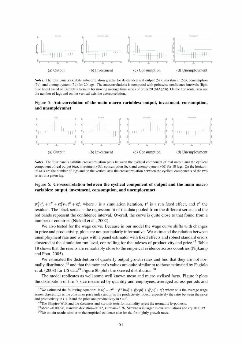
-0.5

00.

000.

501.

00Au

toco

rrela

tions

0 5 10 15 20Lags

Real output

(a) Output

-0.5

00.

000.

501.

00Au

toco

rrela

tions

0 5 10 15 20Lags

Investment (K output)

(b) Investment

-0.50

0.00

0.50

1.00

Autocorrelations

0 5 10 15 20Lags

Consumption

(c) Consumption

-0.40

-0.20

0.00

0.20

0.40

0.60

Autocorrelations

0 5 10 15 20Lags

Unemployment

(d) Unemployment

Notes. The four panels exhibits autocorrelation graphs for de-trended real output (5a), investment (5b), consumption(5c), and unemployment (5d) for 20 lags. The autocorrelations is computed with pointwise confidence intervals (lightblue lines) based on Bartlett’s formula for moving average time series of order 20 (MA(20)). On the horizontal axis arethe number of lags and on the vertical axis the autocorrelation.

Figure 5: Autocorrelation of the main macro variables: output, investment, consumption,and unemploymnet

-1.00

-0.50

0.00

0.50

1.00

-1.00

-0.50

0.00

0.50

1.00

-10 -5 0 5 10Lags

Output

(a) Output

-1.00

-0.50

0.00

0.50

1.00

-1.00

-0.50

0.00

0.50

1.00

-10 -5 0 5 10Lags

Investment

(b) Investment

-1.00

-0.50

0.00

0.50

1.00

-1.00

-0.50

0.00

0.50

1.00

-10 -5 0 5 10Lags

Consumption

(c) Consumption

-1.00

-0.50

0.00

0.50

1.00

-1.00

-0.50

0.00

0.50

1.00

-10 -5 0 5 10Lags

Unemployment

(d) Unemployment

Notes. The four panels exhibits crosscorrelation plots between the cyclical component of real output and the cyclicalcomponent of real output (6a), investment (6b), consumption (6c), and unemployment (6d) for 10 lags. On the horizon-tal axis are the number of lags and on the vertical axis the crosscorrelation between the cyclical components of the twoseries at a given lag.

Figure 6: Crosscorrelation between the cyclical component of output and the main macrovariables: output, investment, consumption, and unemploymnet

αb2 v2

tr + ιb +αb3 vtrι

b + εbt , where r is a simulation iteration, ιb is a run fixed effect, and εb the

residual. The black series is the regression fit of the data pooled from the different series, and thered bands represent the confidence interval. Overall, the curve is quite close to that found from anumber of countries (Nickell et al., 2002).

We also tested for the wage curve. Because in our model the wage curve shifts with changesin price and productivity, plots are not particularly informative. We estimated the relation betweenunemployment rate and wages with a panel estimator with fixed effects and robust standard errorsclustered at the simulation run level, controlling for the indexes of productivity and price.47 Table18 shows that the results are remarkably close to the empirical evidence across countries (Nijkampand Poot, 2005).

We estimated the distribution of quarterly output growth rates and find that they are not nor-mally distributed,48 and that the moment’s values are quite similar to to those estimated by Fagioloet al. (2008) for US data49 Figure 8b plots the skewed distribution.50

The model replicates as well some well known meso and micro stylised facts. Figure 9 plotsthe distribution of firm’s size measured by quantity and employees, averaged across periods and

47We estimated the following equation: ln wrt = αw +β w lnur

t + γw0 cpirt + γw

1 pirt + εrt ; where w is the average wage

across classes, cpi is the consumer price index and pi is the productivity index, respectively the ratio between the priceand productivity in t > 0 and the price and productivity in t = 0.

48The Shapiro-Wilk and the skewness and kurtosis tests for normality reject the normality hypothesis.49Mean=0.00996, standard deviation=0.012, kurtosis=3.76. Skewness is larger in our simulations and equals 0.39.50We obtain results similar to the empirical evidence also for the fortnightly growth rates.

51

-1.0

0-0

.50

0.00

0.50

1.00

-1.0

0-0

.50

0.00

0.50

1.00

-10 -5 0 5 10Lags

Growth of inventories

(a)

-1.0

0-0

.50

0.00

0.50

1.00

-1.0

0-0

.50

0.00

0.50

1.00

-10 -5 0 5 10Lags

Inventories/Sales ratio

(b)

-1.0

0-0

.50

0.00

0.50

1.00

-1.0

0-0

.50

0.00

0.50

1.00

-10 -5 0 5 10Lags

Average wages

(c)

-1.0

0-0

.50

0.00

0.50

1.00

-1.0

0-0

.50

0.00

0.50

1.00

-10 -5 0 5 10Lags

Average mark-up

(d)

Notes. The four panels exhibits cross-correlation plots between the cyclical component of real output and the cyclicalcomponent of inventories growth (7a), inventories/Sales ratio (7b), average wages (7c), and average mark-up (7d) for10 lags. On the horizontal axis are the number of lags and on the vertical axis the crosscorrelation between the cyclicalcomponents of the two series at a given lag.

Figure 7: Crosscorrelation between the cyclical component of output and other aggregatevariables: inventories, wages, prices and mark-up

(a) Beveridge curve

010

2030

40D

ensi

ty

-.02 0 .02 .04 .06Quarterly output growth

(b) Output growth rate distribution

Notes. The left panel (8a) plots the estimation of the Beveridge curve for 60 runs (light grey series) and the estimationof the Beveridge curve for the pooled sample of the 100 series for 1000 time periods. The red band is the confidenceinterval of the aggregate curve. On the horizontal axis is the vacancy ratio (number of vacancies over employment) andon the vertical axis is the unemployment rate. All series are estimated with a polynomial regression of order 2. Theright panel 8b exhibits the real output growth rate distribution (continuous line) against the normal distribution (dashedline) for the average growth rate across the 100 runs.

Figure 8: Beveridge curve and output growth rate distribution

pooled across the 100 series. The plot shows the relation between the log size and the log rank,compared with a log normal distribution with the same average and standard deviation. Bothmeasures show a striking similarity with real data. The final distribution of firms’ size is related totheir growth process, which, as expected, is also not normally distributed and has a high kurtosis.51

The distribution of firm growth emerging from our model is closer to a Laplace distribution thanto a Gaussian distribution (Figure 9c and 9d) although it does not fit perfectly with a Laplacedistribution.

Firms also differ with respect to their productivity and these differences build through timeand tend to be persistent. We plot the time pattern of the productivity series for the “oldest” 14firms surviving until the end of the simulation in a random replication (Figure 10c). All firmstend to maintain their relative position with respect to competitors. Figure 10a plots the averageand standard deviation across all firms across all 100 simulation replicates. The average sharplyincreases, as well as the differences across firms (standard deviation).

5111.3 for quarterly growth rate of output and 7.8 for quarterly growth of employees. For both series the Skew-ness/Kurtosis tests for normality and the Shapiro-Wilk test reject the null hypothesis of normal distribution.

52

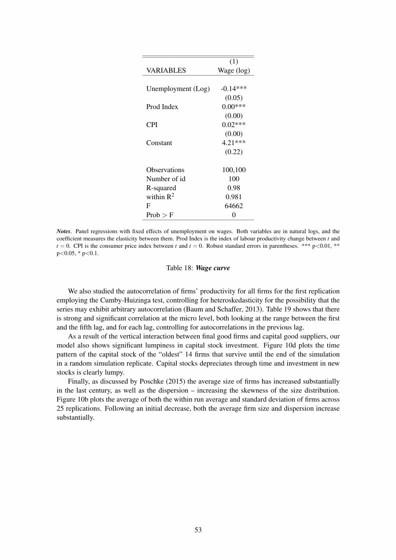
(1)VARIABLES Wage (log)

Unemployment (Log) -0.14***(0.05)

Prod Index 0.00***(0.00)

CPI 0.02***(0.00)

Constant 4.21***(0.22)

Observations 100,100Number of id 100R-squared 0.98within R2 0.981F 64662Prob > F 0

Notes. Panel regressions with fixed effects of unemployment on wages. Both variables are in natural logs, and thecoefficient measures the elasticity between them. Prod Index is the index of labour productivity change between t andt = 0. CPI is the consumer price index between t and t = 0. Robust standard errors in parentheses. *** p<0.01, **p<0.05, * p<0.1.

Table 18: Wage curve

We also studied the autocorrelation of firms’ productivity for all firms for the first replicationemploying the Cumby-Huizinga test, controlling for heteroskedasticity for the possibility that theseries may exhibit arbitrary autocorrelation (Baum and Schaffer, 2013). Table 19 shows that thereis strong and significant correlation at the micro level, both looking at the range between the firstand the fifth lag, and for each lag, controlling for autocorrelations in the previous lag.

As a result of the vertical interaction between final good firms and capital good suppliers, ourmodel also shows significant lumpiness in capital stock investment. Figure 10d plots the timepattern of the capital stock of the “oldest” 14 firms that survive until the end of the simulationin a random simulation replicate. Capital stocks depreciates through time and investment in newstocks is clearly lumpy.

Finally, as discussed by Poschke (2015) the average size of firms has increased substantiallyin the last century, as well as the dispersion – increasing the skewness of the size distribution.Figure 10b plots the average of both the within run average and standard deviation of firms across25 replications. Following an initial decrease, both the average firm size and dispersion increasesubstantially.

53

(a) Size (output) (b) Size (employees)

02

46

810

Den

sity

-.5 0 .5 1 1.5Quarterly output growth

(c) Growth (output)

05

1015

Den

sity

-.5 0 .5 1Quarterly labour growth

(d) Growth (labour)

Notes. The first two plots show the relation between the log of firm size (horizontal axis) and the log of the size rank(vertical axis). Size is measured as firm output (9a) and employment 9b. We pool all firms across the 100 time seriesand average size over the firm life span. Black circles represent the distribution of simulated firms, whereas grey circlesrepresent a log normal distribution. The last two plots show the distribution of firm size quarterly growth with respectto output (9c) and employees (9d).

Figure 9: Log-log plot of firm size distribution

05

1015

200 400 600 800 1000 1200Time

Average Standard deviationConfidence interval

(a) Firm productivity

5000

1000

015

000

2000

025

000

3000

0

200 400 600 800 1000 1200Time

Average Standard deviationConfidence interval

(b) Firm size

810

Firm

pro

duct

ivity

1000 1050 1100 1150 1200 1250Vacancy rate

(c) Productivity: 14firms

1000

0020

0000

3000

0040

0000

5000

0060

0000

Firm

cap

ital s

tock

1000 1050 1100 1150 1200 1250Time

(d) Capital stock: 14firms

Notes. The three panels plot micro regularities across the firms. Panel 10a plots the average and the standard deviationof the productivity of all firms across all 100 simulation replicates. Panel 10b plots the average of the within simulationaverage across 25 simulation runs (with confidence interval) and the average standard deviation within 25 simulationruns. Panel 10c plots the series of the 14 “oldest” firms in the the first simulation replication. Panel 10d plots the capitalstock of 14 “oldest” firms in the the first simulation replication.

Figure 10: Firm productivity, capital, and size

H0: q=0 (serially uncorrelated) H0: q=0 (serially uncorrelated)HA: s.c. present at range specified HA: s.c. present at range specified

lags chi2 df p-val lag chi2 df p-val

1-1 525.306 1 0.00 1 525.306 1 0.001-2 525.309 2 0.00 2 506.186 1 0.001-3 540.39 3 0.00 3 451.117 1 0.001-4 541.171 4 0.00 4 295.336 1 0.001-5 541.877 5 0.00 5 71.669 1 0.00

Notes. Cumby-Huizinga test for autocorrelation for panel data with large sample size (Baum and Schaffer, 2013) underthe null hypothesis of no autocorrelation at any lag order. Test robust to heteroskedasticity. Test also corrected for thepossibility that the series may exhibit arbitrary autocorrelation. The left panel report the lag range (between the firstand the the last period). The panel on the right reports the correlation at each lag.

Table 19: Autocorrelation of firm productivity

54

G Extra Tables

ϑ

0.06 0.07 0.08 0.09 0.10.725; 0.275 89.30*** 96.36** 103.27*** 110.90*** 119.01***0.775; 0.225 84.86*** 93.58 100.05*** 103.97*** 111.82***

λp,1; 0.825; 0.175 80.25*** 88.24*** 94.01 98.46*** 105.54***λq,1 0.875; 0.125 75.27*** 82.21** 89.96*** 94.97 100.63***

0.925; 0.075 70.82*** 78.07*** 84.08*** 89.46*** 95.450.975; 0.025 67.84*** 73.29*** 79.70*** 84.80*** 90.59***

Notes: Mean values over 20 replications for the average inverse herfindahl index over 2000 simulation steps. The indexis computes using sales, across all sectors. The significance of the difference between the benchmark configuration (initalics) and each pair of parameters is computed with a t-test: *** p<0.01, ** p<0.05, * p<0.1

Table 20: Inverse Herfindahl Index for different levels of competition

55

Recent papers in the SPRU Working Paper Series:

June

Explaining Sociotechnical Transitions: A Critical Realist Perspective. Steve Sorrell

Social Innovation, Democracy and Makerspaces. Adrian Smith

Adoption and Diffusion of Micro-Grids in Italy. An Analysis of Regional Factors Using

Agent-Based Modelling. Francesco Pasimeni

May

The Measurement of Synergy in Innovation Systems: Redundancy Generation in a Triple

Helix of University-Industry-Government Relations. Loet Leydesdorff, Henry Etzkowitz,

Inga Ivanova and Martin Meyer

March

Inclusive Innovation and Rapid Sociotechnical Transitions: The Case of Mobile Money in

Kenya. Elsie Onsongo and Johan Schot

Does Managerial Experience Affect Strategic Change? Matte Hartog and Frank Neffke

Coworker Complementarity. Frank Neffke

February

Technical Skills, Disinterest and Non-Functional Regulation: Energy Efficiency Barriers

Viewed in an Ecosystem of Energy Service Companies. Hanna-Liisa Kangas, David

Lazarevic and Paula Kivimaa

Employment Effects of Innovations over the Business Cycle: Firm-Level Evidence from

European Countries. Bernhard Dachs, Martin Hud, Christian Koehler, and Bettina Peters

Policy Democracy: Social and Material Participation in Biodiesel Policy-Making Processes

in India. Evelien de Hoop and Saurabh Arora

January

A Typology of European Research Universities. Differentiation, Layering and Resource

Distribution. Benedetto Lepori, Aldo Geuna and Valerio Veglio

SPRU – Science Policy Research Unit

University of Sussex

Falmer, Brighton, BN1 9SL,United Kingdom

SWPS Website: www.sussex.ac.uk/spru/research/swps

SPRU Website: www.sussex.ac.uk/spru

SPRU Twitter: @SPRU

Suggested citation:

Tommaso Ciarli, André Lorentz, Marco Valente and Maria Savona (2017). StructuralChanges and Growth Regimes. SPRU Working Paper Series (SWPS), 2017-12: 1-55. ISSN

2057-6668. Available at: www.sussex.ac.uk/spru/swps2017-12