Swirling pipe flow with axial strain : experiment and large eddy ...
248
Swirling pipe flow with axial strain : experiment and large eddy simulation Moene, A.F. DOI: 10.6100/IR565932 Published: 01/01/2003 Document Version Publisher’s PDF, also known as Version of Record (includes final page, issue and volume numbers) Please check the document version of this publication: • A submitted manuscript is the author's version of the article upon submission and before peer-review. There can be important differences between the submitted version and the official published version of record. People interested in the research are advised to contact the author for the final version of the publication, or visit the DOI to the publisher's website. • The final author version and the galley proof are versions of the publication after peer review. • The final published version features the final layout of the paper including the volume, issue and page numbers. Link to publication Citation for published version (APA): Moene, A. F. (2003). Swirling pipe flow with axial strain : experiment and large eddy simulation Eindhoven: Technische Universiteit Eindhoven DOI: 10.6100/IR565932 General rights Copyright and moral rights for the publications made accessible in the public portal are retained by the authors and/or other copyright owners and it is a condition of accessing publications that users recognise and abide by the legal requirements associated with these rights. • Users may download and print one copy of any publication from the public portal for the purpose of private study or research. • You may not further distribute the material or use it for any profit-making activity or commercial gain • You may freely distribute the URL identifying the publication in the public portal ? Take down policy If you believe that this document breaches copyright please contact us providing details, and we will remove access to the work immediately and investigate your claim. Download date: 17. Feb. 2018
Transcript of Swirling pipe flow with axial strain : experiment and large eddy ...

Swirling pipe flow with axial strain : experiment and largeeddy simulationMoene, A.F.
DOI:10.6100/IR565932
Published: 01/01/2003
Document VersionPublisher’s PDF, also known as Version of Record (includes final page, issue and volume numbers)
Please check the document version of this publication:
• A submitted manuscript is the author's version of the article upon submission and before peer-review. There can be important differencesbetween the submitted version and the official published version of record. People interested in the research are advised to contact theauthor for the final version of the publication, or visit the DOI to the publisher's website.• The final author version and the galley proof are versions of the publication after peer review.• The final published version features the final layout of the paper including the volume, issue and page numbers.
Link to publication
Citation for published version (APA):Moene, A. F. (2003). Swirling pipe flow with axial strain : experiment and large eddy simulation Eindhoven:Technische Universiteit Eindhoven DOI: 10.6100/IR565932
General rightsCopyright and moral rights for the publications made accessible in the public portal are retained by the authors and/or other copyright ownersand it is a condition of accessing publications that users recognise and abide by the legal requirements associated with these rights.
• Users may download and print one copy of any publication from the public portal for the purpose of private study or research. • You may not further distribute the material or use it for any profit-making activity or commercial gain • You may freely distribute the URL identifying the publication in the public portal ?
Take down policyIf you believe that this document breaches copyright please contact us providing details, and we will remove access to the work immediatelyand investigate your claim.
Download date: 17. Feb. 2018

Swirling pipe flow with axial strain
Experiment and Large Eddy Simulation
Arnold F. Moene

ii
Copyright ©2003, Arnold F. Moene
CIP-DATA LIBRARY TECHNISCHE UNIVERSITEIT EINDHOVEN
Moene, Arnold Frank
Swirling pipe flow with axial strain : experiment and large eddy simulation / Arnold FrankMoene. – Eindhoven : Technische Universiteit Eindhoven, 2003. –Proefschrift.ISBN 90-386-1695-3NUGI 926Trefw.: stroming ; pijpleidingen / interne turbulente stroming / roterende stroming / axiale ver-vorming / laser-Doppler anemometrie / numerieke simulatieSubject headings: pipe flow / swirling flow / axial strain / turbulence / laser-Doppler velocimetry/ Large Eddy Simulation

Swirling pipe flow with axial strain
Experiment and Large Eddy Simulation
PROEFSCHRIFT
ter verkrijging van de graad van doctor aan de Technische Universiteit Eindhoven, opgezag van de Rector Magnificus, prof.dr. R.A. van Santen, voor een commissieaangewezen door het college voor promoties in het openbaar te verdedigen op
donderdag 19 juni 2003 om 16.00 uur
Arnold F. Moene
geboren te Amsterdam

iv
Dit proefschrift is goedgekeurd door de promotoren:prof.dr.ir. G.J.F. van Heijstenprof.dr.ir. F.T.M. Nieuwstadt

Contents
1 Introduction 11.1 Turbulent swirling flow with axial strain . . . . . . . . . . . . . . . . . . . . . . 11.2 Methodology of turbulence research . . . . . . . . . . . . . . . . . . . . . . . . 3
1.2.1 General . . . . . . . . . . . . . . . . . . . . . . . . . . . . . . . . . . . 31.2.2 This study . . . . . . . . . . . . . . . . . . . . . . . . . . . . . . . . . . 3
1.3 Aims of this research . . . . . . . . . . . . . . . . . . . . . . . . . . . . . . . . 41.4 Outline of the thesis . . . . . . . . . . . . . . . . . . . . . . . . . . . . . . . . . 6
2 Turbulence subject to swirl and axial strain 92.1 Turbulence and basic equations . . . . . . . . . . . . . . . . . . . . . . . . . . . 9
2.1.1 Navier-Stokes equations . . . . . . . . . . . . . . . . . . . . . . . . . . 92.1.2 Phenomena in turbulent flows . . . . . . . . . . . . . . . . . . . . . . . 102.1.3 Reynolds-averaged equations . . . . . . . . . . . . . . . . . . . . . . . 122.1.4 Equations for the Reynolds-stresses . . . . . . . . . . . . . . . . . . . . 132.1.5 Equations for incompressible flow in a cylindrical geometry . . . . . . . 14
2.2 Swirl . . . . . . . . . . . . . . . . . . . . . . . . . . . . . . . . . . . . . . . . . 142.2.1 The link between phenomena in swirling flows . . . . . . . . . . . . . . 152.2.2 Streamline curvature and stability . . . . . . . . . . . . . . . . . . . . . 172.2.3 Rotation . . . . . . . . . . . . . . . . . . . . . . . . . . . . . . . . . . . 192.2.4 Three-dimensionality . . . . . . . . . . . . . . . . . . . . . . . . . . . . 212.2.5 Swirl decay . . . . . . . . . . . . . . . . . . . . . . . . . . . . . . . . . 22
2.3 Axial strain . . . . . . . . . . . . . . . . . . . . . . . . . . . . . . . . . . . . . 232.3.1 Effect of axial strain on mean flow . . . . . . . . . . . . . . . . . . . . . 242.3.2 Effect of axial strain on turbulence . . . . . . . . . . . . . . . . . . . . . 252.3.3 Relaxation of strained flow . . . . . . . . . . . . . . . . . . . . . . . . . 27
2.4 Combined effect of swirl and axial strain . . . . . . . . . . . . . . . . . . . . . . 282.4.1 Inviscid analysis of simplified swirling flows subject to axial strain . . . . 282.4.2 Turbulent flows with swirl and axial strain . . . . . . . . . . . . . . . . . 30
2.5 To conclude . . . . . . . . . . . . . . . . . . . . . . . . . . . . . . . . . . . . . 32
3 Laser Doppler measurements 353.1 Principles of Laser Doppler Anemometry . . . . . . . . . . . . . . . . . . . . . 35
3.1.1 Fundamentals . . . . . . . . . . . . . . . . . . . . . . . . . . . . . . . . 363.1.2 Implementation . . . . . . . . . . . . . . . . . . . . . . . . . . . . . . . 393.1.3 Error sources . . . . . . . . . . . . . . . . . . . . . . . . . . . . . . . . 41
3.2 Experimental set-up . . . . . . . . . . . . . . . . . . . . . . . . . . . . . . . . . 42
v
vi Contents
3.2.1 Pipe system . . . . . . . . . . . . . . . . . . . . . . . . . . . . . . . . . 433.2.2 LDA system: optics, positioning and data processing . . . . . . . . . . . 46
3.3 Measurement strategy . . . . . . . . . . . . . . . . . . . . . . . . . . . . . . . . 543.3.1 Flow types . . . . . . . . . . . . . . . . . . . . . . . . . . . . . . . . . 543.3.2 Processed data . . . . . . . . . . . . . . . . . . . . . . . . . . . . . . . 553.3.3 Raw data . . . . . . . . . . . . . . . . . . . . . . . . . . . . . . . . . . 56
4 Numerical simulation of turbulence 574.1 Principles of Large Eddy Simulation . . . . . . . . . . . . . . . . . . . . . . . . 58
4.1.1 Filtering the governing equations . . . . . . . . . . . . . . . . . . . . . 584.1.2 The relationship between filtering and the SGS-model . . . . . . . . . . 604.1.3 Subgrid scale-stress modelling . . . . . . . . . . . . . . . . . . . . . . . 614.1.4 Solution of the Navier-Stokes equations: some numerical issues . . . . . 684.1.5 Comparison between LES results and laboratory experiments . . . . . . 714.1.6 Sources of error in LES . . . . . . . . . . . . . . . . . . . . . . . . . . . 71
4.2 An LES model for pipe flow with swirl and axial strain . . . . . . . . . . . . . . 724.2.1 Coordinate system . . . . . . . . . . . . . . . . . . . . . . . . . . . . . 734.2.2 Spatial discretisation . . . . . . . . . . . . . . . . . . . . . . . . . . . . 744.2.3 Temporal discretisation and pressure solution . . . . . . . . . . . . . . . 754.2.4 Sub-grid scale model . . . . . . . . . . . . . . . . . . . . . . . . . . . . 774.2.5 Boundary conditions . . . . . . . . . . . . . . . . . . . . . . . . . . . . 78
4.3 Strategy of the simulations . . . . . . . . . . . . . . . . . . . . . . . . . . . . . 82
5 Analysis of laboratory measurements 855.1 Mean flow and Reynolds stresses: data . . . . . . . . . . . . . . . . . . . . . . . 85
5.1.1 A note on the presentation of data . . . . . . . . . . . . . . . . . . . . . 855.1.2 Flow with axial strain and no swirl . . . . . . . . . . . . . . . . . . . . . 865.1.3 Flow with axial strain and swirl . . . . . . . . . . . . . . . . . . . . . . 91
5.2 Mean flow and Reynolds stresses: analysis . . . . . . . . . . . . . . . . . . . . . 995.2.1 Interpretation of the observations . . . . . . . . . . . . . . . . . . . . . 995.2.2 Development of the swirl number . . . . . . . . . . . . . . . . . . . . . 1035.2.3 Three-dimensionality in swirling flow . . . . . . . . . . . . . . . . . . . 1065.2.4 Comparison of stress-anisotropy between non-swirling and swirling flow 1065.2.5 Rapid distortion analysis of normal stresses at centreline . . . . . . . . . 112
5.3 Analysis of time series data . . . . . . . . . . . . . . . . . . . . . . . . . . . . . 1165.3.1 Spectra . . . . . . . . . . . . . . . . . . . . . . . . . . . . . . . . . . . 1165.3.2 Integral scales . . . . . . . . . . . . . . . . . . . . . . . . . . . . . . . . 119
5.4 To conclude . . . . . . . . . . . . . . . . . . . . . . . . . . . . . . . . . . . . . 1205.4.1 Axial strain without swirl . . . . . . . . . . . . . . . . . . . . . . . . . 1205.4.2 Axial strain with swirl . . . . . . . . . . . . . . . . . . . . . . . . . . . 121

Contents vii
6 Results of numerical simulations 1236.1 Validation of the LES results . . . . . . . . . . . . . . . . . . . . . . . . . . . . 123
6.1.1 A note on the presentation of results . . . . . . . . . . . . . . . . . . . . 1236.1.2 Flow with axial strain . . . . . . . . . . . . . . . . . . . . . . . . . . . . 1246.1.3 Flow with swirl and axial strain . . . . . . . . . . . . . . . . . . . . . . 126
6.2 Further analysis of LES results . . . . . . . . . . . . . . . . . . . . . . . . . . . 1386.2.1 Velocity and stress fields . . . . . . . . . . . . . . . . . . . . . . . . . . 1386.2.2 Budgets for turbulent stresses . . . . . . . . . . . . . . . . . . . . . . . 1416.2.3 Stress anisotropy at the pipe axis . . . . . . . . . . . . . . . . . . . . . . 1566.2.4 Axial development of the swirl number . . . . . . . . . . . . . . . . . . 157
6.3 To conclude . . . . . . . . . . . . . . . . . . . . . . . . . . . . . . . . . . . . . 1586.3.1 Axial strain without swirl . . . . . . . . . . . . . . . . . . . . . . . . . 1586.3.2 Axial strain with swirl . . . . . . . . . . . . . . . . . . . . . . . . . . . 159
7 Conclusion 1617.1 Current knowledge . . . . . . . . . . . . . . . . . . . . . . . . . . . . . . . . . 1617.2 Experimental results . . . . . . . . . . . . . . . . . . . . . . . . . . . . . . . . 162
7.2.1 Axial strain without swirl . . . . . . . . . . . . . . . . . . . . . . . . . 1627.2.2 Axial strain with swirl . . . . . . . . . . . . . . . . . . . . . . . . . . . 162
7.3 Development of LES model and validation . . . . . . . . . . . . . . . . . . . . . 1637.3.1 Development . . . . . . . . . . . . . . . . . . . . . . . . . . . . . . . . 1637.3.2 Validation . . . . . . . . . . . . . . . . . . . . . . . . . . . . . . . . . . 164
7.4 LES results . . . . . . . . . . . . . . . . . . . . . . . . . . . . . . . . . . . . . 1657.4.1 Axial strain without swirl . . . . . . . . . . . . . . . . . . . . . . . . . 1657.4.2 Axial strain with swirl . . . . . . . . . . . . . . . . . . . . . . . . . . . 165
7.5 Perspectives . . . . . . . . . . . . . . . . . . . . . . . . . . . . . . . . . . . . . 166
A Statistical analysis of turbulent data 169A.1 Averages . . . . . . . . . . . . . . . . . . . . . . . . . . . . . . . . . . . . . . . 169
A.1.1 Reynolds decomposition . . . . . . . . . . . . . . . . . . . . . . . . . . 169A.1.2 Types of averages . . . . . . . . . . . . . . . . . . . . . . . . . . . . . . 169
A.2 Statistical errors . . . . . . . . . . . . . . . . . . . . . . . . . . . . . . . . . . . 171A.2.1 Statistics derived from series of independent samples . . . . . . . . . . . 171A.2.2 Statistics derived from a continuous series . . . . . . . . . . . . . . . . . 172A.2.3 Statistics derived from discretely sampled series . . . . . . . . . . . . . 172A.2.4 Extension of error estimates to averaging in more dimensions . . . . . . 173
A.3 Estimation of statistical errors in LDA data and LES results . . . . . . . . . . . . 173A.3.1 LDA data . . . . . . . . . . . . . . . . . . . . . . . . . . . . . . . . . . 173A.3.2 LES fields . . . . . . . . . . . . . . . . . . . . . . . . . . . . . . . . . . 174

viii Contents
B Auxiliary equations 177B.1 Equations in cylindrical coordinates . . . . . . . . . . . . . . . . . . . . . . . . 177
B.1.1 Navier-Stokes equations . . . . . . . . . . . . . . . . . . . . . . . . . . 177B.1.2 Reynolds stress budget equations . . . . . . . . . . . . . . . . . . . . . 177
B.2 Equations in spectral space . . . . . . . . . . . . . . . . . . . . . . . . . . . . . 180B.2.1 Navier-Stokes equations in spectral space . . . . . . . . . . . . . . . . . 181B.2.2 Reynolds stress budget equations . . . . . . . . . . . . . . . . . . . . . 181
C On the relationship between streamline curvature and rotation in swirling flows 183C.1 Two reference frames . . . . . . . . . . . . . . . . . . . . . . . . . . . . . . . . 183C.2 Application to swirling flows . . . . . . . . . . . . . . . . . . . . . . . . . . . . 184
C.2.1 Solid-body rotation without an axial velocity component . . . . . . . . . 184C.2.2 Solid-body rotation including an axial velocity component . . . . . . . . 185C.2.3 General rotation including an axial velocity component . . . . . . . . . . 185
D Errors in LDA measurements due to geometrical uncertainties 187D.1 Error due to imperfection of theodolite calibration . . . . . . . . . . . . . . . . . 187D.2 Errors due to imperfections of the positioning of the LDA . . . . . . . . . . . . . 187
D.2.1 Rotation around the x1-axis . . . . . . . . . . . . . . . . . . . . . . . . 188D.2.2 Rotation around the x2-axis . . . . . . . . . . . . . . . . . . . . . . . . 188D.2.3 Rotation around the x3-axis . . . . . . . . . . . . . . . . . . . . . . . . 188
D.3 Errors in 3D measurements . . . . . . . . . . . . . . . . . . . . . . . . . . . . . 188D.4 Application of error estimates . . . . . . . . . . . . . . . . . . . . . . . . . . . 189
E Details on the LES model 191E.1 Example of equations in transformed coordinates . . . . . . . . . . . . . . . . . 191E.2 Example of spatial discretisation: divergence . . . . . . . . . . . . . . . . . . . 191E.3 Details on boundary conditions . . . . . . . . . . . . . . . . . . . . . . . . . . . 193
E.3.1 Implementation of wall boundary condition for ur . . . . . . . . . . . . . 193E.3.2 Implementation of wall boundary condition for p′ . . . . . . . . . . . . 193
E.4 Details on the radial grid spacing . . . . . . . . . . . . . . . . . . . . . . . . . . 194E.5 Test of methods to generate swirl . . . . . . . . . . . . . . . . . . . . . . . . . . 195
F Dependence of simulations of developed pipe flow on size and shape of the grid 201F.1 Grid size dependence . . . . . . . . . . . . . . . . . . . . . . . . . . . . . . . . 201F.2 Grid shape dependence . . . . . . . . . . . . . . . . . . . . . . . . . . . . . . . 203
G Wiggles or oscillations in Large Eddy Simulation of swirling pipe flow 207G.1 Introduction . . . . . . . . . . . . . . . . . . . . . . . . . . . . . . . . . . . . . 207G.2 Wiggles . . . . . . . . . . . . . . . . . . . . . . . . . . . . . . . . . . . . . . . 207
G.2.1 Role of mesh-Reynolds number . . . . . . . . . . . . . . . . . . . . . . 207G.2.2 Aliasing . . . . . . . . . . . . . . . . . . . . . . . . . . . . . . . . . . . 208
G.3 Solutions . . . . . . . . . . . . . . . . . . . . . . . . . . . . . . . . . . . . . . 209
Contents ix
G.4 Conclusion . . . . . . . . . . . . . . . . . . . . . . . . . . . . . . . . . . . . . 211
H Pressure strain terms in turbulent flow through an axially rotating pipe 213H.1 Intro . . . . . . . . . . . . . . . . . . . . . . . . . . . . . . . . . . . . . . . . . 213H.2 Models for the pressure strain tensor . . . . . . . . . . . . . . . . . . . . . . . . 213H.3 The flow and the simulation . . . . . . . . . . . . . . . . . . . . . . . . . . . . . 216H.4 Results . . . . . . . . . . . . . . . . . . . . . . . . . . . . . . . . . . . . . . . . 216
H.4.1 Simulation results . . . . . . . . . . . . . . . . . . . . . . . . . . . . . 216H.4.2 Results on the parameterisations . . . . . . . . . . . . . . . . . . . . . . 216
H.5 Conclusion . . . . . . . . . . . . . . . . . . . . . . . . . . . . . . . . . . . . . 217
References 221
Samenvatting 231
Dankwoord 235
Curriculum Vitae 237

x Contents

1 Introduction
1.1 Turbulent swirling flow with axial strainThe three ingredients in the title of this section are depicted in figure 1.1: turbulence, swirland axial strain. Turbulent flows are irregular, both in space and time. On one hand the fluidis in chaotic motion and is mixed efficiently. On the other hand there is some structure in themotion: fluctuations appear both at short time scales and longer time scales. Swirling flowsare characterised by the fact that the fluid rotates around an axis that is parallel to the mainflow direction. This results in a cork-screw type of motion. Strain is the deformation of asubstance: the relative positions of particles change. In the case of axial strain the deformationis composed only of extension and compression (no shear). As an example, figure 1.1 showsaxially symmetric axial strain: extension in one direction, compression in the two perpendiculardirections.
Swirling flows may either occur inadvertently and be considered as a disturbance (Steenber-gen and Voskamp, 1998) or may be generated on purpose. Applications of swirling flows includecyclone separators, swirling spray dryers, swirling furnaces, vortex tubes used for thermal sep-aration, agitators etc. (Kuroda and Ogawa, 1986). The combination of swirl and axial strainoccurs in a number of industrial applications. In axial cyclone separators a contraction may beused to enhance the rotation in the inlet region. In cyclone separators, based on recirculation, acontraction is used to enhance the return flow and ensure that material that is gathered near thecentre will flow upward, whereas the heavier material near the wall leaves the separator at thelower end (see e.g. figure 1.2). Other situations in which both swirl and axial strain occur arevarious parts of turbomachinery. In those cases the axial strain may either have the form of acontraction or a diffuser. The combination of swirling flow and a diffuser is also used for thestabilisation of flames in combustion chambers.
Understanding of flows in configurations like those mentioned before can be obtained bymeasurements: experimental determination of the velocity field, wall pressure, temperatures or
0 0.1 0.2 0.3 0.4 0.5 0.6 0.7 0.8 0.9 10.15
0.2
0.25
0.3
0.35
0.4
0.45
0.5
0.55
velo
city
(m
/s)
time (seconds)
Figure 1.1: The three ingredients of this thesis: turbulence (left), swirl (centre) and axial strain (right).
1

2 Introduction
flow
light material
heavy material
swirl generator
heavy material
tangential inlet light material
Figure 1.2: Sketches of cyclone separators: axial cyclone (left) and a tangential cyclone (right).
concentrations. However, there may be configurations in which measurements are difficult, ifnot impossible, or certain quantities may be hard to measure. Furthermore, it may happen thatone needs to predict the flow in a not yet existing geometry. In those cases one needs to makea model of the flow. The main complication in such a model is how the turbulent character ofthe flow should be treated. Although it is becoming possible to fully calculate turbulent flows(in three dimensions and time-dependent), this is feasible only at low to moderate Reynoldsnumbers, and in simple geometries. Therefore, one usually reverts to a statistical descriptionof the turbulence. This implies that the fluctuating quantities are characterised by their means,variances, covariances and possibly higher order moments, and models need to be devised thatlink those statistical quantities (see chapter 4). This is the research area of turbulence modelling.
In the context of turbulence modelling swirling flows with axial strain are considered ’com-plex flows’ according to the definition of Bradshaw (1975):
... flows howse turbulence structure is affected by extra rates of strain (velocitygradients) in addition to the simple shear ∂U/∂y, or by body forces: these effects aresurprisingly large and can be spectacular.
The complexity of these flows is further discussed in chapter 2. It suffices here to state that, al-though increasingly successful, current turbulence models still have difficulty with some aspectsof complex flows (e.g. Launder (1989) and Jakirlic et al. (2000)).

1.2 Methodology of turbulence research 3
1.2 Methodology of turbulence research1.2.1 GeneralFigure 1.3 gives a possible picture how different activities in turbulence research may be inter-related. Three different, but interrelated, ways of investigating turbulent flows be distinguished:theory, experiments and modelling. First, the left part of figure 1.3 is considered. Why are the-ories about turbulent flows developed in the first place? The answer is that theories may help tounderstand the processes that occur in a flow. This in turn may help to predict flows in –moreor less– different configurations or conditions. Theoretical studies may rely on the governingequations, simplifications thereof, similarity reasoning or otherwise. But usually the develop-ment of theories will be inspired by experimental observations. Furthermore, once a theory hasbeen developed, experimental results are needed to validate it. Finally, theoretical insights maylead to the development of models for a flow (in terms of parameterisations).
The next focus is on the role of experiments in turbulence research. In the first place, theymay lead to more understanding of a flow, provided that the experiment has been designed suchthat the boundary conditions and initial conditions are well controlled. As mentioned before,experimental results may serve both as inspiration and validation for theories about the flowunder consideration. Similarly, experimental results may also feed the development of turbulencemodels, often in terms of the determination of constants in a theoretical parametrisation (e.g.the Von Karman constant). Experimental validation should always be the final step in modeldevelopment. Besides, experimental validation is useful when a model is applied to a flow thatis slightly or grossly beyond the conditions for which it was developed.
Finally, the attention is focused on the role of models in turbulence research. Again, theseare used to understand flows. One particular advantage of models over experiments is that theflow conditions in a model can be controlled extremely well. This opens the way to so-calledparameter studies, in which important parameters in the flow are varied over a large range to seein which way the characteristics of the flow change. In that way models may also contributeto the development of theories. Especially, the results of Large Eddy Simulation (LES) andDirect Numerical Simulations (DNS) models are useful, since those give detailed spatial andtemporal information on all variables in a flow. This information is (with a few exceptions)not accessible with experimental techniques. In some areas, LES and DNS results are alreadyconsidered as pseudo-data (and thus would belong to the central panel in figure 1.3). Anotherimportant application of turbulence models is of course the prediction of practical flows. This isessential in the design of whatever structure or apparatus in which fluid flow is an issue.
1.2.2 This studyIn the present study, only a subset of the activities sketched in figure 1.3 is present (see figure 1.4).The emphasis in this thesis is on experimentation and numerical simulation. The experiment isused to
• gain insight into the flow under consideration;• validate theory;• provide validation data for the numerical simulations.

4 Introduction
Figure 1.3: Sketch of relationships between different domains of turbulence research. In some casesthe domains may not be as separate as sketched here: e.g. some theories about flows (e.g.K-diffusion theory) could as well be classified as models.
The numerical simulations in turn are used to
• better understand the flow, since they provide more and different data than the experiment;• provide information on new flows, once the model is validated.
1.3 Aims of this researchThe main objective of this thesis is to gain insight into the physics and modelling of turbulentswirling pipe flow with axial strain. More specifically, the configuration studied is the turbulentswirling pipe flow through a contraction (see figure 1.5).
The main objective can be translated into the following research questions:
• What is the current knowledge on the separate subjects of flows with swirl or axial strain,and on the combined effect of swirl and axial strain on turbulent flows?
• Which features and mechanisms can be derived from experimental data of swirling flowwith axial strain, both in comparison to data without swirl but with strain, and in terms ofReynolds number effects? Apart from the conclusions drawn from the experimental data inthis thesis, the data will be relevant as a benchmark for turbulence modellers as well.
• Which modifications need to be made to a Large Eddy Simulation model to apply it to aswirling flow with axial strain, and how well do the results match experimental data?
• Which features and mechanisms can be derived from LES results of turbulent (swirling)flow with axial strain?

1.3 Aims of this research 5
Figure 1.4: Sketch of the place of the present thesis in turbulence research.
flow
flow
5.8 D31 D
6 D1.8 D
Figure 1.5: Configuration of the flow studied: swirling flow through a pipe contraction. Bottom: thedomain of study for the laboratory experiment. Top: the domain used for the numericalsimulations. Dimensions are expressed in the pipe diameter upstream of the contraction, D(70 mm); the pipe diameter downstream of the contraction is 40 mm.

6 Introduction
Figure 1.6: Overview of the setup of this thesis. Not included are the introduction and the conclusion,as well as the appendices.
1.4 Outline of the thesisThe outline of this thesis is sketched in figure 1.6. Following this introduction, the thesis contin-ues with a review of literature on various aspects of the flow under consideration, viz. turbulence,swirl, axial strain and the combined effect of swirl and axial strain (chapter 2). Then two chaptersare devoted to the experimental and modelling techniques used:
• chapter 3 deals with the theory behind the experimental technique used: Laser DopplerAnemometry (LDA), and describes the experimental setup used in this study;
• chapter 4 highlights some relevant aspects of LES and describes the development of an LESmodel capable of simulating a swirling flow through a contraction.
The next two chapters present the results of the laboratory experiment and the numerical simu-lations:
• chapter 5 starts with a presentation and discussion of the laboratory results of the flowsstudied: swirling and non-swirling flow, both with axial strain. In the second part of thechapter the results are analysed in the light of the theoretical aspects presented in chapter 2.

1.4 Outline of the thesis 7
• chapter 6 starts with a validation of the LES results, for swirling and non-swirling flow withaxial strain. In the second part of the chapter those results of the LES are presented thathave not been (and could not be) measured in the laboratory experiment.
Finally, chapter 7 concludes this thesis with a synthesis of the results of the previous chaptersand a perspective of what could be the following steps.
This thesis contains a fair number of appendices that provide details for issues discussed inthe respective chapters:
• Appendix A on statistical analysis of turbulent data supports chapters 2, 5 and 6.• Appendix B presents some elaborate equations and supports chapters 2, 5 and 6• Appendix C discusses the link between rotation and streamline curvature, two aspects of
swirling flow that are dealt with in chapter 2.• Appendix D summarises the results of Steenbergen (1995) regarding the errors in measured
mean velocities and stresses, due to geometrical uncertainties in the experimental setup(relevant for chapters 3 and 5).
• Appendix E gives details on the LES model not covered in chapter 4.• Appendices F and G discuss two numerical issues that surfaced during the development of
the LES model (chapter 4).• Appendix H presents the results of a separate study in which a Direct Numerical Simulation
of a turbulent flow through a rotating pipe has been analysed. Although the configuration isdifferent from the subject of this study, it is sufficiently related to warrant its inclusion.

8 Introduction

2 Turbulence subject to swirland axial strain
In the introductory chapter (section 1.1) the relevance was argued of turbulent flows in which bothswirl and axial strain play a role. In order to better understand the dynamics of these types offlow, a first step is to highlight the various ingredients that contribute to this flow, i.e. turbulence(section 2.1), swirl (2.2) and axial strain (2.3). After understanding the contributing phenomenaa complete picture of ‘swirling turbulent pipe flow subject to axial strain’ is expected to evolve:Section 2.4 discusses what is known at this moment of the combined effect of swirl and axialstrain, and section 2.5 aims to summarise this chapter.
2.1 Turbulence and basic equationsFor more than a century turbulent flows have been studied, and this has resulted in many, more orless commonly accepted, views on the nature of turbulence. However, none of the descriptions ofturbulent flows has been successful in explaining all aspects of this flow (Tennekes and Lumley,1972). In this section an introduction to the main aspects of turbulent flows will be given. Thisintroduction is not meant to be exhaustive, but rather to provide the concepts and tools neededin forthcoming sections. For more information and details on turbulent flows the reader is re-ferred to the numerous introductory and advanced textbooks that exist on the topic of turbulence.Examples are Tennekes and Lumley (1972), Hinze (1975) and Lesieur (1993).
The introduction starts with the presentation of the equations governing fluid flow. Subse-quently phenomena and concepts regarding turbulent flows will be discussed. Finally, one tech-nique to tackle the complexity of turbulent flows will be considered in more detail, i.e. thestatistical description. The equations that describe the statistical properties of a turbulent floware presented at the end of this section.
2.1.1 Navier-Stokes equationsIn the case of an isothermal fluid, the fluid flow can be described with two conservation laws: theconservation of mass and the conservation of momentum. If it is furthermore assumed that theflow is incompressible, i.e. the density does not vary with pressure (Kundu, 1990), and that thereare no other sources of density variations, the continuity equation reduces to:
∇∇∇ · uuu = 0 , (2.1)
where uuu is the velocity vector.The conservation of momentum for a Newtonian fluid, assuming incompressibility, can be
9

10 Turbulence subject to swirl and axial strain
expressed as:
∂uuu∂t+∇∇∇ · uuuuuu = −1
ρ∇∇∇p +∇∇∇ · νSSS (2.2)
where ρ is the density of the fluid, p is the pressure, ν is the kinematic viscosity and SSS is thestrain rate tensor1: SSS = 1
2
(∇∇∇uuu + (∇∇∇uuu)T
). Since in an isothermal fluid the viscosity is constant and
∇∇∇·uuu = 0, the term∇∇∇·νSSS can be replaced by ν∇2uuu. The resulting equation is known as the Navier-Stokes equation. Equations (2.1) and (2.2) form a system of four differential equations with fourvariables: the pressure and three components of the velocity vector. Given appropriate initial andboundary conditions and taking the pressure gradient as a parameter rather than a variable2, theseequations can be solved in principle, although the number of flows for which this is possible inpractice is limited due to the non-linearity of the momentum equations.
The standard way to investigate the relative importance of the terms in (2.2), typical scales areassigned to all variables. Variables normalised by these typical scale are then expected to yielddimensionless variables that are of order 1. For the velocities a typical scale U is used, and thelengths are scaled with L . The pressure is scaled using the velocity scale as ρU2 and the timescale is constructed as L/U. The dimensionless version of a variable (say x) is denoted by x.The scaled —dimensionless– version of (2.2) becomes (after division byU2/L):
∂uuu
∂t+∇∇∇ · uuuuuu = −∇∇∇ p +
ν
UL∇∇∇ · νSSS , (2.3)
The inverse of the factor ν/(UL) is known as the Reynolds number Re. When Re is large theviscous term does not play an important role, whereas the viscous term dominates over the non-linear term when Re is small. The Reynolds number will be large when either the length scaleor the velocity scale (or both) of a flow are large (e.g. a planetary boundary layer with a lengthscale of 1000 m and a velocity scale of 5 ms−1). Low Reynolds numbers will occur in the case ofsmall length scales and velocity scales (e.g. flow of water through soil pores and the flow closeto a wall).
2.1.2 Phenomena in turbulent flowsStarting with the pioneering work of Reynolds (1895), turbulent flows have been the subject ofscientific research ever since (see e.g. Monin and Yaglom, 1971, for a review). Based on thisresearch a more or less commonly accepted picture has evolved that describes turbulent flowsboth qualitatively and quantitatively. Based on this picture some general properties of turbulentflows can be summarised (after Tennekes and Lumley (1972); Lesieur (1993)):
1The product∇∇∇uuu is a so-called dyad. A general example is the dyad AAA = aaabbb: a second order tensor with elementsAi j = aib j. Although the notation used in Spencer (1988): AAA = aaa ⊗ bbb is clearer in distinguishing between differenttypes of products, the notation AAA = aaabbb will be used for reasons of compactness. In general aaabbb , bbbaaa = (aaabbb)T .The gradient of a vector could be denoted either by ∇∇∇aaa ( ∂
∂xia j in Cartesian coordinates) or aaa∇∇∇ ( ∂
∂x jai in Cartesian
coordinates) , but the latter form would be confusing, so we will write (∇∇∇aaa)T instead. More information about dyadscan be found in Phillips (1948) and Aris (1989).
2Where in a compressible flow the equations of state could be used as an independent equation for the pressure,there is no such equation in an incompressible flow. However, by taking the divergence of the momentum equationsand using the continuity equation a Poisson equation for the pressure results. See section 4.2.3 for more information.

2.1 Turbulence and basic equations 11
a. Turbulence occurs in flows at high Reynolds numbers: i.e. the non-linear terms in thegoverning equations dominate over the linear viscous terms (see (2.2)).
b. Turbulent flows are irregular or chaotic in space and time3: they are not reproducible indetail.
c. Turbulent flows are diffusive : heat, momentum, as well as mass are mixed and transportedefficiently by turbulent flows. In many practical applications this is a desirable feature ofturbulence.
d. Turbulence is essentially rotational and three-dimensional, which is a distinction to otherchaotic flows. Rotating patches of fluid (loosely called eddies ) have length scales rangingfrom the size of the flow domain down to the order of millimetres (see below for details).
e. Turbulent flows are dissipative: the kinetic energy of the velocity fluctuations, producedat the largest scales, is dissipated at the smallest scales into heat through viscous diffusion(the Reynolds number is of order unity at this scale).
Whether a flow is turbulent or laminar depends on characteristics of both the fluid (i.e. theviscosity) and the flow (the velocity scale and length scale of the flow). Both factors are combinedin the Reynolds number. When the Reynolds number exceeds a certain value the flow in generalbecomes unstable and turbulence develops 4.
As stated above, turbulent eddies can have sizes that span a large range of length scales. Atthe large-scale end of the spectrum eddies occur that have a length scale L (∼ 0.1-1 times thedomain size), a velocity scale U(∼ square root of the turbulent kinetic energy) and a time scaleT (= L/U). The smallest scales on the other hand are related to the length scale at which theturbulent kinetic energy is dissipated (η, see below). The large scales lose energy at a rate (ε)that is totally determined by large-scale properties:
ε =U3
L(2.4)
The flow adjusts in such a way that the velocity fluctuations at the smallest scale are able todissipate the amount of energy supplied by the large scales5. Thus the length scale of the smallesteddies, η, as well as the related velocity scale (v) and time scale (τm) only depend on ε and ν. In
3Chaotic is not equivalent to random or white noise: in turbulent flows correlations do exist over certain distancesin time and space (see further in this section)
4For a pipe flow —for example— a logical choice for U would be the bulk velocity U b and the pipe diameterD for L. Then the value of ReD above which the flow is turbulent has been found experimentally to be about 2300,given that sufficient disturbances are present in the flow. But laminar pipe flows have been observed at Reynoldsnumbers of the order of 50000 (Schlichting, 1979; Draad, 1996). The process of transition from a laminar flowto turbulence is a complicated matter, which will not be discussed here. A lower bound for ReD, below which noturbulent flow will exist is about 2000.
5Dissipation is more efficient at smaller scales, since velocity gradients are relatively large. Dissipation is alsomore efficient if viscosity is larger.

12 Turbulence subject to swirl and axial strain
terms of dimensional analysis this leads to the following estimates for these scales:
η =(ν3/ε
)1/4(2.5a)
v = (νε)1/4 (2.5b)
τm = η/v = (ν/ε)1/2 (2.5c)
When a Reynolds number is formed based on small-scale length and velocity scales (Reε = ηv/ν)we see that this exactly equals 1, thus indicating that at the smallest scales viscous processesdominate.
In order to study the relationship between the characteristic scales of the large-scale and small-scale motion, (2.4) and (2.5) are combined to yield:
η
L= Re−3/4
L (2.6a)
vU= Re−1/2
L (2.6b)
τm
T= Re−1/4
L (2.6c)
It can be seen that with increasing ReL the range of length scales increases, as well as the rangeof time scales and velocity scales. This is particularly relevant for the numerical simulation ofturbulence: the spatial discretisation will be of the order of η whereas the total flow domain has
a size L. Thus the total number of grid points in three dimensions will be of the order of(Re3/4
L
)3
and the number of time steps (as far as this is limited by turbulent time scales) will grow as Re1/4L .
2.1.3 Reynolds-averaged equationsSince turbulent flows are not reproducible in detail, and since one is usually not interested in thesedetails, one needs to revert to a statistical description of the flow. This is done by a Reynoldsdecomposition of all variables (remind that the density is taken to be constant and thus is not avariable in the present case):
a = a + a′ , (2.7)
where x denotes the ensemble average of a and x′ is the deviation from the ensemble average.6
First (2.7) is applied to the continuity equation (2.1) and the resulting equation is ensembleaveraged again:
∇∇∇ · uuu +∇∇∇ · uuu′ = ∇∇∇ · uuu = 0 . (2.8)
Thus the ensemble average field is divergence free.
6For more details on the subject of ensemble averaging and the relation with other types of averages, the readeris directed to Appendix A.
2.1 Turbulence and basic equations 13
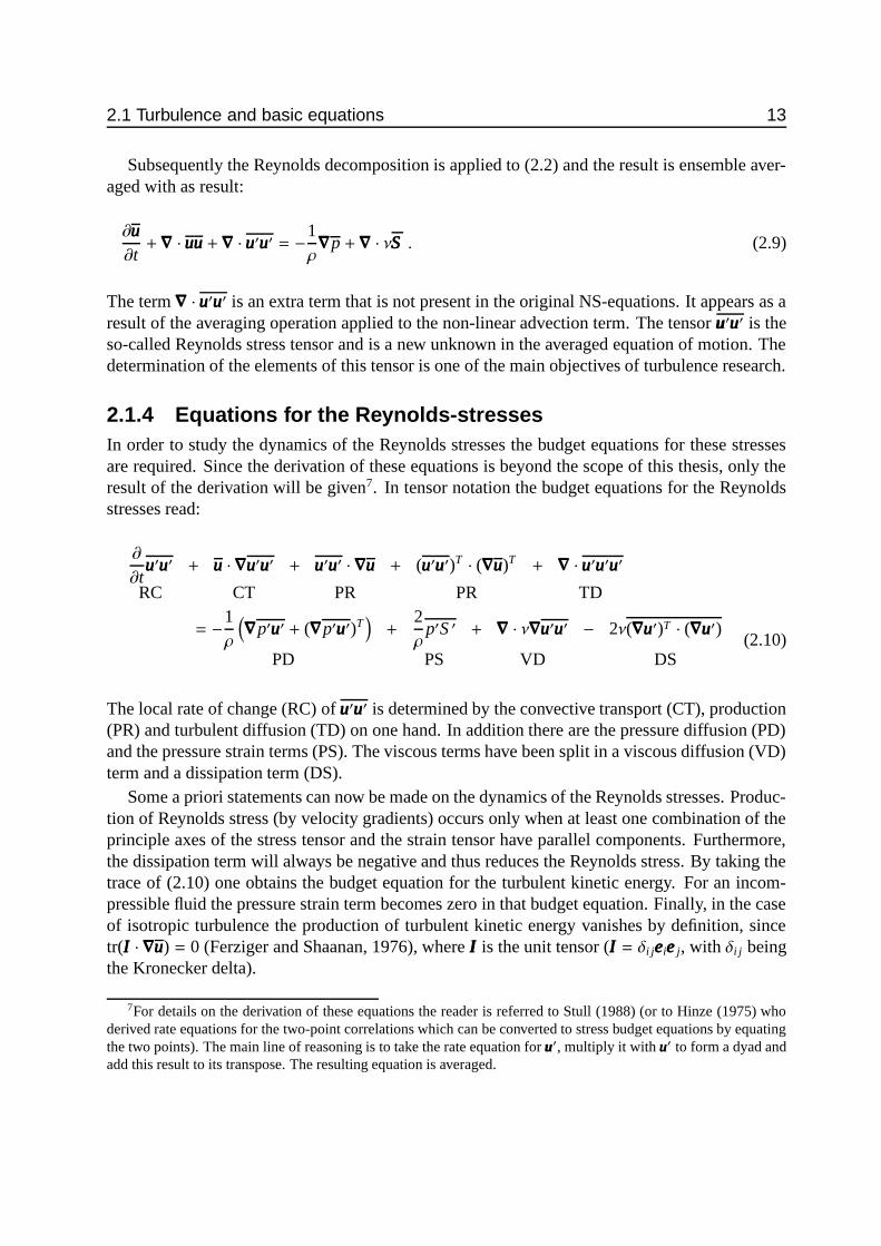
Subsequently the Reynolds decomposition is applied to (2.2) and the result is ensemble aver-aged with as result:
∂uuu∂t+∇∇∇ · uuuuuu +∇∇∇ · uuu′uuu′ = −1
ρ∇∇∇p +∇∇∇ · νSSS . (2.9)
The term ∇∇∇ · uuu′uuu′ is an extra term that is not present in the original NS-equations. It appears as aresult of the averaging operation applied to the non-linear advection term. The tensor uuu′uuu′ is theso-called Reynolds stress tensor and is a new unknown in the averaged equation of motion. Thedetermination of the elements of this tensor is one of the main objectives of turbulence research.
2.1.4 Equations for the Reynolds-stressesIn order to study the dynamics of the Reynolds stresses the budget equations for these stressesare required. Since the derivation of these equations is beyond the scope of this thesis, only theresult of the derivation will be given7. In tensor notation the budget equations for the Reynoldsstresses read:
∂
∂tuuu′uuu′ + uuu · ∇∇∇uuu′uuu′ + uuu′uuu′ · ∇∇∇uuu + (uuu′uuu′)T · (∇∇∇uuu)T
+ ∇∇∇ · uuu′uuu′uuu′
RC CT PR PR TD
= −1ρ
(∇∇∇p′uuu′ + (∇∇∇p′uuu′)T
)+
2ρ
p′S ′ + ∇∇∇ · ν∇∇∇uuu′uuu′ − 2ν(∇∇∇uuu′)T · (∇∇∇uuu′)
PD PS VD DS(2.10)
The local rate of change (RC) of uuu′uuu′ is determined by the convective transport (CT), production(PR) and turbulent diffusion (TD) on one hand. In addition there are the pressure diffusion (PD)and the pressure strain terms (PS). The viscous terms have been split in a viscous diffusion (VD)term and a dissipation term (DS).
Some a priori statements can now be made on the dynamics of the Reynolds stresses. Produc-tion of Reynolds stress (by velocity gradients) occurs only when at least one combination of theprinciple axes of the stress tensor and the strain tensor have parallel components. Furthermore,the dissipation term will always be negative and thus reduces the Reynolds stress. By taking thetrace of (2.10) one obtains the budget equation for the turbulent kinetic energy. For an incom-pressible fluid the pressure strain term becomes zero in that budget equation. Finally, in the caseof isotropic turbulence the production of turbulent kinetic energy vanishes by definition, sincetr(III · ∇∇∇uuu) = 0 (Ferziger and Shaanan, 1976), where III is the unit tensor (III = δi jeeeieee j, with δi j beingthe Kronecker delta).
7For details on the derivation of these equations the reader is referred to Stull (1988) (or to Hinze (1975) whoderived rate equations for the two-point correlations which can be converted to stress budget equations by equatingthe two points). The main line of reasoning is to take the rate equation for uuu′, multiply it with uuu′ to form a dyad andadd this result to its transpose. The resulting equation is averaged.
14 Turbulence subject to swirl and axial strain
2.1.5 Equations for incompressible flow in a cylindrical geometrySince the geometry of the flow domain we aim to consider here has axial symmetry, use will bemade of cylindrical coordinates throughout this study. The cylindrical coordinate system is de-fined by the three coordinates z , θ and r (the axial, tangential and radial coordinate, respectively).The velocity vector uuu is decomposed into the components along these coordinate directions: uz,uθ and ur, respectively.
The Reynolds averaged continuity equation (2.1) can now be expressed as:
∇∇∇ · uuu = 1r∂ru[r]∂r
+1r∂u[θ]∂θ+∂u[z]∂z
(2.11)
The next step is to derive the Reynolds averaged equations of motion, which can be found inHinze (1975):
∂ur
∂t+
(uuu · ∇∇∇) ur −
uθ2
r= −1
ρ
∂p∂r+
1r∂rτrr
∂r+
1r∂τrθ
∂θ+∂τrz
∂z− τθθ
r(2.12a)
∂uθ∂t+
(uuu · ∇∇∇) uθ +
uruθr= − 1
ρr∂p∂θ+
1r∂rτrθ
∂r+
1r∂τθθ
∂θ+∂τzθ
∂z+τrθ
r(2.12b)
∂uz
∂t+
(uuu · ∇∇∇) uz = −
1ρ
∂p∂z+
1r∂rτrz
∂r+
1r∂τθz
∂θ+∂τzz
∂z(2.12c)
with
τ = σσσ −
u′r2 u′ru
′θ
u′ru′z
u′ru′θ
u′θ
2 u′θu′z
u′ru′z u′θu′z u′z
2
(2.12d)
σσσ = νSSS (2.12e)
The Navier-Stokes equations in cylindrical coordinates are given in section B.1.1, whereas thebudget equations for the Reynolds stresses are given in section B.1.2.
2.2 SwirlThe term ‘swirling flow’ indicates a very loosely defined class of flows. The main characteristicthat all swirling flows have in common is that the flow has both an axial velocity component anda tangential velocity component (Kuroda and Ogawa, 1986). Swirling flows can be both confined(pipe flow or flow between two coaxial cylinders) and free flows (jet). Given the subject of thisthesis, the emphasis in the following discussions will be on confined swirling flows.
A rough classification of swirling flows can be made, based on the shape of the tangentialvelocity profile (Kitoh, 1991; Steenbergen, 1995):

2.2 Swirl 15
radial position
tang
entia
l vel
ocity
0
0
(a)
0
0
0
0
radial position
tang
entia
l vel
ocity
(b)
radial position
tang
entia
l vel
ocity
0
0
(c)
radial position
tang
entia
l vel
ocity
0
0
(d)
Figure 2.1: Tangential velocity profiles for a number of prototype swirling flows: forced vortex (a), freevortex (b), Rankine vortex (c) and wall jet (d).
• Forced vortex or solid-body rotation;• Free vortex, which is irrotational;• Rankine vortex, which is a combination of a forced vortex in the centre and a free vortex
in the outer part; when the transition between from the forced vortex to the free vortex issmoother, the uθ-profile resembles that of a Burgers vortex (a diffusing line vortex in axialstrain) after some diffusion occurred.
• Wall jet, in which the maximum tangential velocity occurs near the wall.
A sketch of the tangential velocity profiles for these prototypes is given in figure 2.1 (thesesketches refer to a confined flow)8. The extent of the core with positive vorticity, as well as thelocation of the maximum vorticity depends on the type of swirl.
Swirling flows unify a number of complexities which occur in other turbulent flows as well:streamline curvature, rotation and three-dimensionality. Furthermore, the rotation may decaydownstream due to friction: swirl decay. These phenomena will be the subjects of separatesections, but before discussing these topics separately, an attempt will be made to show the linkbetween them in section 2.2.1.
2.2.1 The link between phenomena in swirling flowsThe first feature of swirling flows is the non-zero mean tangential velocity. A flow without axialvelocity, leads to the circular streamline pattern shown in figure 2.2(a). This streamline patternpossesses two related characteristics: streamline curvature and rotation. The effects of thesephenomena on turbulence are the subject of quite distinct volumes of literature. This distinction isprobably due to the difference in the origin of the interest in streamline curvature versus rotation:aerodynamics versus geophysical flows. For the current discussion, however, it is sufficient tonotice that the distinction is a human invention –related to the choice of reference frame– ratherthan a physical reality (see for appendix C for a limited discussion on this topic).
8Note that in the case of a pipe flow with swirl a core with positive vorticity (in axial direction) exists in thecentral part, whereas near the wall a shear region with vorticity of opposite sign can be found.
16 Turbulence subject to swirl and axial strain
(a)
uz
(b)
uz
(c)
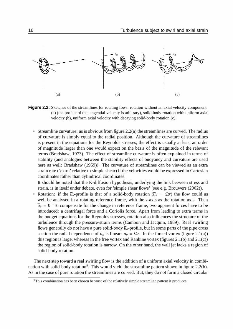
Figure 2.2: Sketches of the streamlines for rotating flows: rotation without an axial velocity component(a) (the profile of the tangential velocity is arbitrary), solid-body rotation with uniform axialvelocity (b), uniform axial velocity with decaying solid-body rotation (c).
• Streamline curvature: as is obvious from figure 2.2(a) the streamlines are curved. The radiusof curvature is simply equal to the radial position. Although the curvature of streamlinesis present in the equations for the Reynolds stresses, the effect is usually at least an orderof magnitude larger than one would expect on the basis of the magnitude of the relevantterms (Bradshaw, 1973). The effect of streamline curvature is often explained in terms ofstability (and analogies between the stability effects of buoyancy and curvature are usedhere as well: Bradshaw (1969)). The curvature of streamlines can be viewed as an extrastrain rate (‘extra’ relative to simple shear) if the velocities would be expressed in Cartesiancoordinates rather than cylindrical coordinates.It should be noted that the K-diffusion hypothesis, underlying the link between stress andstrain, is in itself under debate, even for ’simple shear flows’ (see e.g. Brouwers (2002)).
• Rotation: if the uθ-profile is that of a solid-body rotation (uθ = Ωr) the flow could aswell be analysed in a rotating reference frame, with the z-axis as the rotation axis. Thenuθ = 0. To compensate for the change in reference frame, two apparent forces have to beintroduced: a centrifugal force and a Coriolis force. Apart from leading to extra terms inthe budget equations for the Reynolds stresses, rotation also influences the structure of theturbulence through the pressure-strain terms (Cambon and Jacquin, 1989). Real swirlingflows generally do not have a pure solid-body uθ-profile, but in some parts of the pipe crosssection the radial dependence of uθ is linear: uθ = Ωr. In the forced vortex (figure 2.1(a))this region is large, whereas in the free vortex and Rankine vortex (figures 2.1(b) and 2.1(c))the region of solid-body rotation is narrow. On the other hand, the wall jet lacks a region ofsolid-body rotation.
The next step toward a real swirling flow is the addition of a uniform axial velocity in combi-nation with solid-body rotation9. This would yield the streamline pattern shown in figure 2.2(b).As in the case of pure rotation the streamlines are curved. But, they do not form a closed circular
9This combination has been chosen because of the relatively simple streamline pattern it produces.
2.2 Swirl 17
path, but have become spirals. The radius of curvature now not only depends on the distancefrom the centre of rotation, but on the axial velocity as well (in the limit of infinite axial velocitythe streamline curvature would disappear). Still, both the analysis in terms of turbulence in arotating frame, and in terms of streamline curvature are valid. The fact that the streamlines areno longer parallel gives rise to three-dimensionality. This implies that the fluid is distorted orsheared in the cross-flow direction10.
The effects of streamline curvature, rotation and three-dimensionality are only three of a longlist of ‘extra strain rates’ given by Bradshaw (1973)11. Bradshaw uses the term ‘extra rate ofstrain’ in his qualitative discussions for ‘any departure from simple shear’. In the case of swirlingpipe flow the ‘simple shear’ (or one-dimensional shear) would be ∂
∂r uz. The streamline curva-ture is expressed in the shear −uθ/r Three-dimensionality is present when the shear ∂
∂r uθ is notproportional to ∂
∂r uz.A final aspect of swirling flows is the decay of swirl: the total amount of tangential momen-
tum decreases due to wall friction. Figure 2.2(c) shows the streamlines in the idealised case ofuniform axial velocity and a decaying solid-body rotation. In terms of extra rates of strain, thedecay of swirl introduces two new complications: the axial changes in uz and uθ give rise to extrashears: ∂
∂zuz and ∂∂zuθ. However, it should be noted that the decay of swirl is a slow process in
most cases, and then the axial derivatives will generally be negligible, compared to other extrastrains or shears (which are due to streamline curvature and three-dimensionality).
The phenomena in swirling flows summarised above will be the subject of the forthcomingsections.
2.2.2 Streamline curvature and stabilityFor a thorough review of the research until the early 1970’s on the effects of streamline curvaturethe reader is referred to Bradshaw (1973). More recent reviews can be found in Bradshaw (1990)and Holloway and Tavoularis (1992). A detailed overview of linear stability analysis can befound in Schlichting (1979).
Here the main emphasis will be on the influence of streamline curvature on the stability offlows. The term ‘stability’ can here be interpreted in two ways:
• The stability of a basic mean flow is analysed in terms of the growth or decay of distur-bances that are added to the basic flow. These disturbances may be subject to constraints onsymmetry or dimensionality. This type of —linear— stability analysis is most often used tostudy the transition to turbulence, or the formation of secondary flows;
• The stability of turbulent flows is can be analysed in terms of the growth or suppression ofthe turbulent kinetic energy , or in terms of the change of the anisotropy of the stress tensor,in an already turbulent flow.
Both interpretations of stability will be dealt with below.
10In some flows, regions may exist where ∂∂r uz ∼ ∂
∂r uθ (for example in the outer region of the free vortex and Rank-ine vortex, see figures 2.1(b) and 2.1(c)). In that case the flow could be considered to be locally two-dimensional.
11The term ‘extra strain rate’ is rather inexact: the list of Bradshaw not only includes strains (= deformation) butshears (deformation and rotation) and pure rotation as well.

18 Turbulence subject to swirl and axial strain
Stability in terms of growth of disturbances
The applicability of linear stability analysis to turbulent flows is limited since the turbulent fluc-tuations are usually much larger than the ‘small’ disturbances on which linear stability analysisis based. Besides, if linear stability analysis predicts the growth of a disturbance, this growthmay be obscured by the turbulent fluctuations that are present already. On the other hand, iflinear stability analysis predicts stability, this may be visible in a turbulent flow as a damping offluctuations (provided of course that the flow remains turbulent: the Reynolds number remainsabove the critical Reynolds number).
The notion that the curvature of streamlines may have either a stabilising or a destabilisingeffect on fluid flow dates back at least to Rayleigh (1916). His main conclusion —based on atwo-dimensional, inviscid analysis— is that the flow between two coaxial cylinders, of which atleast one is rotating, is unstable when the angular momentum (uθr) increases outward. This isthe so-called centrifugal instability. The argument of Rayleigh in fact boils down to a ‘displacedparticle’ argument. Various versions of the ‘displaced particle’ argument exist of which someconsider the effect of solid-body rotation on a shear flow, where the rotation axis is perpendicularto the shear plane, (Tritton, 1992; Cambon et al., 1994). Others consider the effect of streamlinecurvature in a shear flow (Rayleigh, 1916; Bradshaw, 1973; Lumley et al., 1985). All theseanalyses have in common that they are purely two-dimensional and inviscid. The stability offlows which include an axial velocity component has been analysed by Leibovich and Stewartson(1983) in the context of vortex breakdown and by Mackrodt (1976) and Pedley (1969) for aHagen-Poisseuille flow in a rotating pipe.
The analysis of Rayleigh (1916) of the stability of the flow between two concentric cylin-ders was extended by Taylor (1923) to include viscosity and three-dimensional perturbations.It appears that the presence of viscosity stabilises the flow. The instabilities that occur are thewell-known Taylor vortices: counter-rotating toroidal vortices. An instability that is more closelyrelated to swirling pipe flow (but also related to the Taylor vortices) is the instability of a bound-ary layer over a concavely curved surface. This instability gives rise to the the so-called Taylor-Gortler vortices (Schlichting, 1979). In the application of the above —linear and viscous—stability analyses it should be remembered that in those flows the instability occurs, before theflow becomes fully turbulent. Thus in fully turbulent flows the patterns predicted by the theorymay be obscured by non-linear instabilities and interactions.
Stability in terms of the growth of turbulence quantities
Streamline curvature also has a profound influence on turbulence quantities. In particular atten-tion has been paid to the effect of curvature on the shear stress in shear flows. Prandtl (1961)focuses on turbulent flows and draws an analogy between flows influenced by buoyancy andflows in which streamline curvature produces the (de-)stabilising effect. He proposes to modifythe expression for the turbulent shear stress, based on his mixing-length theorem, with a factordepending on the stability, expressed in the dimensionless number S , which is defined as (not to
2.2 Swirl 19
be confused with the swirl number or strain tensor)12:
S =uθr
(∂uθ∂r− uθ
r
)−1
(2.13)
This S can be interpreted as the ratio between work done by (or against) the centrifugal forceand the work done by the mean flow (shear) on the turbulence. In this sense it is similar to aRichardson number which describes the influence of buoyancy on the production of turbulentkinetic energy. For a profile with uθ(r) = const/r the curvature can be seen to have no effect.,whereas for profiles with uθ(r) ∼ rn with n < −1 Prandtl predicts instability and for n > −1stability. Bradshaw (1969) has investigated the analogy between the stability effects of streamlinecurvature and buoyancy in more depth.
As opposed to the stability analyses presented above, Holloway and Tavoularis (1998) statethat the effects of mild streamline curvature on the anisotropy of the Reynolds stress tensor do notarise from a centrifugal effect. They present a geometric explanation instead. In this explanationit is assumed that a turbulent eddy maintains its original orientation once it has been produced.In a curved flow this implies that the axes of the eddy will rotate relative to the coordinates of thecurved flow. The orientation of the eddies that are found at a certain position in the flow is thecumulative effect of eddies that have been convected from various positions upstream (and havedecayed in the meantime).
For a review of experimental evidence for the effect of streamline curvature on turbulent(shear) the reader is referred to Holloway and Tavoularis (1992).
2.2.3 RotationWhen a turbulent flow is considered in a rotating reference frame the Reynolds averaged mo-mentum equations have to be augmented with two apparent accelerations: the centrifugal forceand the Coriolis force:
∂uuu∂t+∇∇∇ · uuuuuu +∇∇∇ · uuu′uuu′ = −1
ρ∇∇∇p +∇∇∇ · νSSS + Ω2RRR − 2ΩΩΩ × uuu . (2.14)
/see b where ΩΩΩ is the rotation vector, Ω is the magnitude of ΩΩΩ, and RRR is the distance betweenthe point of interest and the rotation axis. The centrifugal force is balanced by an increasedpressure gradient force. The Coriolis force causes an exchange of momentum between differentcomponents of the velocity vector. Another influence of the rotation enters (2.14) through theReynolds stress, which is influenced by rotation as well (see below).
In order to gain some extra insight, the perspective of two-point statistics of the velocityfield is needed, e.g. the Fourier transform of the velocity field. Jacquin et al. (1990) showthat under certain conditions, an inertial wave regime results (see also Veronis, 1970) which
12In the original paper the dimensionless number was called θ. The form of the function proposed by Prandtl forthe stability effect of buoyancy is remarkably close to relationships found experimentally in the 1960’s (see Garrat(1992) for a review). But the magnitude of the effect is an order of magnitude larger than expected by Prandtl, whichis in line with the statements of Bradshaw (1973). See also Bradshaw (1969) for the analogy between stability effectsof curvature and buoyancy.

20 Turbulence subject to swirl and axial strain
corresponds to ‘spring-like’ behaviour observed by Johnston et al. (1972) and to the ‘displacedparticle analysis’ by Tritton (1992) (see section 2.2.2). One of the effects of these inertial wavesis the disruption of the phase relations in turbulence, so-called phase-scrambling. This hampersthe energy cascade and —since the small scales just dissipate the energy delivered by the largerscales— also diminishes the dissipation (see Zhou, 1995).
A next step is to study the direct effect of rotation on the budget equation for the Reynoldsstress (equation (2.10)). Two extra terms occur in this equation due to the rotation:
RC + CT + PR + TD = PD + PS + VD + DS − 2ΩΩΩ × uuu′uuu′ − 2(ΩΩΩ × uuu′uuu′)T (2.15)
The effect of the extra terms is to generate an exchange between different components of thestress tensor. Or, equivalently, the principal axes of the stress tensor are rotated around therotation axis. In section 2.1.4 (equation (2.10)) it was shown that the angle between the straintensor and the stress tensor determines the production of Reynolds stresses (Bertoglio, 1982), sothat rotation does —indirectly— influence that production. The effect of rotation on the turbulentkinetic energy can be studied by taking the trace of (2.15). It appears that the rotation terms donot have a direct contribution ((ΩΩΩ × uuu′) · uuu′ = 0 since ΩΩΩ × uuu′ ⊥ uuu′). However, by changingthe relative magnitude of the different stress components, the rotation terms do influence theturbulent kinetic energy indirectly through the production terms.
In the analysis of (2.15) the influence of rotation on the pressure diffusion term, pressure strainterm and the turbulent diffusion remains unclear. Some extra understanding can be obtainedby analysing the effect of rotation on the Fourier transform of the Reynolds stress tensor, i.e.the spectral tensor ΦΦΦ. In these analyses the role of a part of the pressure-strain terms can bestudied. Cambon and Jacquin (1989) studied the influence of rotation on homogeneous butanisotropic turbulence. They find that rotation enhances the anisotropy of the length scales,while it diminishes the difference between the normal stress components parallel and normal tothe rotation axis.
Bertoglio (1982) and Cambon et al. (1994) study the effect of rotation on homogeneous tur-bulence that includes mean shear. They analyse the flow in terms of the rotation number R:
Rn =2Ωω
(2.16)
where ω is the vorticity of the (ensemble) mean flow. They find that maximum destabilisationof the flow occurs at Rn = −1/2 or zero tilting vorticity (Cambon et al., 1994)13. The destabili-sation occurs mainly through the pressure strain terms. If Rn > 0 the mean rotation adds to therotation of the shear and stabilisation occurs. Tritton (1992) arrives at the same conclusion usinga simplified Reynolds stress model, and assuming that the principal axes of uuu′uuu′ and Duuu′uuu′/Dtare aligned.
This section concludes with some (laboratory and numerical) experimental evidence of theinfluence of rotation of turbulent flows. Three similar experiments, studying the influence ofrotation on grid-generated turbulence, have been performed by Traugott (1958), Wigeland (1978)
13Due to an unfortunate definition of the direction of the rotation vector Ω in his paper, Bertoglio (1982) statesthat the maximum destabilisation occurs for Rn = 1/2, rather than Rn = −1/2.

2.2 Swirl 21
and Jacquin et al. (1990). Although these experiments do contradict each other in some places —which may be attributed to experimental deficiencies— the main conclusions stand out clearly:
• Rotation reduces the dissipation of the turbulent kinetic energy;• The effect of rotation on anisotropic turbulence is highly dependent on the exact form of the
anisotropy;• The length scales along the mean flow direction tend to increase with rotation, the effect
being more pronounced for the length scale of the radial component.
Bardina et al. (1985) find in numerical simulations of rotating isotropic turbulence that thelength scales become anisotropic due to rotation. All length scales grow, but the length scalesof the velocity components perpendicular to the rotation axis grow more. Rotation also hasa large effect on dissipation14: the vortex tubes are reordered to become more parallel to therotation axis, which hampers the energy cascade. Bardina et al. interpret this modification ofthe energy cascade in terms of a conversion of turbulent energy into inertial waves. Mansouret al. (1992) have performed direct numerical simulations and EDQNM (Eddy-Damped Quasi-Normal Markovian) computations of isotropic turbulence subject to strong rotation. Their resultsalso show a shut-off of the energy transfer from large scales to small scales. Anisotropy in theturbulent length scales is observed for intermediate rotation rates only. For strong rotation notendency toward two-dimensionality can be observed.
2.2.4 Three-dimensionalityIn case of a simple shear flow the magnitude of the mean velocity varies in a direction perpen-dicular to that mean velocity (in most cases this direction is normal to a wall). In the context offluid flow three-dimensionality refers to a situation in which not only the magnitude of the meanvelocity varies (shear) but also the direction of the mean velocity changes in a direction normalto the mean velocity vector (Schlichting, 1979).
Nearly all research on three-dimensionality in turbulent flows has focused on three-dimensionalboundary layers. Various processes may be responsible for the occurrence of three-dimensionalboundary layers. These comprise:
• the bounding surface moves laterally relative to the mean flow direction (e.g. Bissonette andMellor, 1974);
• due to some upstream disturbance the mean velocity has a lateral component for a range ofdistances normal to the wall (swirling pipe flow belongs to this category);
• the presence of an obstacle in a flow over a flat surface; the obstacle will influence thepressure field upstream, which will in turn influence the velocity field (e.g. Hornung andJoubert, 1962);
• differences in downstream boundary layer development may produce a lateral pressure gra-dient and subsequent three-dimensionality (e.g. ’swept-wing’ experiments (by e.g. van denBerg et al., 1975)).
14Dissipation can be viewed as the interaction of randomly oriented vortex tubes. The tubes need to have a certainmutual orientation to be able to exchange momentum efficiently.
22 Turbulence subject to swirl and axial strain
One of the differences between a standard shear layer and a three-dimensional boundary layeris that the directions of mean velocity (γ), shear (γg) and stress (γτ) do not need to coincide(and will not do so in general). The angles are γ, γg, and γτ are defined in a plane parallel tothe bounding surface. Examples can be found in literature where the difference between γg andγτ is of the order of 10 degrees. The difference between γ and γg is even larger (see van denBerg, 1988; Bradshaw and Pontikos, 1985; Bruns et al., 1999). The implication of shear andstress not being aligned is that the eddy-viscosity is anisotropic (the component in the cross-flow direction being the smallest). The alignment of shear and stress in a simple shear flow(one-dimensional shear) is often considered to be an indication of local equilibrium betweenproduction and dissipation. On the other hand, the non-alignment in the case of a steady three-dimensional boundary layer may point at a non-local equilibrium and history effects in the flowmight be important (van den Berg, 1988).
Another effect that has been observed in three-dimensional boundary layers is a general re-duction in the shear stress relative to the turbulent kinetic energy (Compton and Eaton, 1997).This might be explained by so-called ’turbulent eddy toppling’ (Bradshaw and Pontikos, 1985).This term refers to the process that large turbulent eddies –with sizes comparable to the boundarylayer depth– are distorted and even disrupted by the cross-flow shear acting on them.
In the context of swirling flows, it should be noted that the effect of three-dimensionality inthe near-wall region appears to be of minor importance. Only at distances beyond approximatelyy+ = 60 the flow gradually becomes skewed (Kitoh, 1991).
2.2.5 Swirl decayIn a wall-bounded swirling flow, the tangential motion will decay downstream due to a tangentialwall shear stress15. This tangential wall shear stress will of course have a pronounced effect onthe shape of the profiles of both the mean velocities and the turbulent stresses. However, in thecase of swirl decay most attention is paid to the decay of the total ’amount of swirl’. Numerousintegral quantities have been devised to represent this amount of swirl. Here the swirl number(S ) as given by Kitoh (1991) (see also Steenbergen and Voskamp (1998)) will be used:
S = 2∫ R
0
uzuθr2
Ubulk2R3
dr (2.17)
This swirl number is equal to the non-dimensionalised angular momentum flux (i.e. the axialflux of angular momentum).
The amount of swirl decreases downstream due to the loss of mean tangential momentumthrough the tangential wall shear stress. By integration of the mean momentum equation for uθ(multiplied by r2), an expression for the tangential wall shear stress in terms of uz, uθ, u′zu
′θ
and∂∂zuθ can be obtained (for axisymmetric flow):
τrθ,wall
ρ=
1R2
∫ R
0r2 ∂
∂z
(uzuθ + u′zu
′θ− ν∂uθ
∂z
)dr (2.18)
15Unless it is a flow in which the swirl is generated by the rotation of the pipe wall itself Imao et al. (1996);Eggels (1994).

2.3 Axial strain 23
uzuθ will be much larger than both u′zu′θ
and ν ∂uθ∂z . With this knowledge, and by scaling all veloci-
ties by Ubulk, and the axial coordinate by the pipe diameter D, (2.18) can be rewritten as:
τrθ,wall
12ρUbulk
2= 2
dd(x/D)
∫ R
0
uzuθr2
Ubulk2R3
dr =12
dSd(x/D)
(2.19)
Then Kitoh (1991) suggests to express τrθ,wall as a series expansion in terms of S . For low swirlnumbers one can decide to only retain the linear term, i.e. τrθ,wall ∼ S . In that case an exponentialdecay law for S is obtained:
S = ae−βz/D , (2.20)
where a and β are fitting coefficients. The quantity a can be interpreted as a the swirl number atthe axial position z = 0 and β is the a measure of the decay rate16. This approximate exponentialdecay has been confirmed experimentally for many types of swirling flows, although the decayrates (i.e. β) do depend on the type of flow and to some extent on the swirl number. Besides, thereis a dependence of β on ReD: the decay depends on the scaled tangential wall shear stress whichappears to have the same dependence on ReD as the scaled axial wall shear stress τrz,wall/ρUbulk
2.The latter is related to the Re-dependence of the friction factor λ = (8u∗/Ubulk)2. Steenbergen(1995) finds for low initial swirl numbers (of O(0.2)) that β = (1.49 ± 0.07)λ. Note that thefriction factor used here is the λ for a fully developed pipe flow, as given by Blasius’ relationship:0.3168Re−1/4
D . An ample review of swirl decay rates obtained in 18 other experiments is given inSteenbergen and Voskamp (1998).
Although most analyses of swirling flows are based on the assumption that the flow is ax-isymmetric (so that all angular momentum is present in uθ and not in ur), asymmetries do occurin practice. Kito (1984) concludes that small asymmetries in the inflow can result in large asym-metries further downstream. Furthermore, Kito considers the precession of the vortex core (i.e.the axial change in the location of the vortex core in the pipe cross section). He suggests that thedirection of precession is always in in the same direction as the swirl (0 < S < 0.4). However,Dellenback et al. (1988) show that for 0 < S < 0.15 the precession direction is opposite to theswirl and for higher S it is in the same direction.
2.3 Axial strainThe term axial strain signifies one of many possible strain configurations, among which are planestrains and combinations of axial strain and plane strain (see Reynolds and Tucker (1975)). Inan axial strain the flow is strained (in the mean) in its flow direction. This can be expressed in amean strain rate tensor SSS (in Cartesian coordinates) as:
SSS =
D 0 00 − 1
2 D 00 0 − 1
2 D
, (2.21)
16Generally, a is not equal to S at z = 0, since the decay process is not exponential in the initial stage.
24 Turbulence subject to swirl and axial strain
where D =∂ux1∂x1
. In a wall bounded flow an axial strain can easily be generated by means of adownstream change in the cross-sectional area of the flow domain. This change in cross-sectionalarea can either be a locally continuous decrease (contraction) or increase (diffuser) or decreasefollowed by an increase (constriction). In a contraction the flow is accelerated, whereas in adiffuser the flow is decelerated.
Two aspects will influence the strain that is realised in practice:
• The friction at the wall will locally influence the strain field;• The way in which the cross-sectional area changes with axial position determines whether
–and in which way– the strain varies with the axial position in the contraction.
In the sequel, only contractions will be considered, since that is the type of axial strain genera-tor used in the present study. Thus the studies on flows through diffusers and constrictions will beleft out (e.g. Cantrak (1981); Spencer et al. (1995); Desphande and Giddens (1980); Lissenburget al. (1974)).
The study of the turbulent flow through pipe contractions has been motivated by differentneeds. On one hand, contractions, diffusers and constrictions are present in all kinds of pipingsystems (industrial applications, water supply systems, etc; see Bullen et al. (1996)). In theseapplications the main interest is in the pressure loss due to the presence of the change in pipediameter, and the possible occurrence of separation (see section 2.3.1). On the other hand, the ax-ial strain due to a change in pipe diameter also strongly influences the turbulence structure. Thiseffect has practical applications, since some processes in industrial installations, such as mixing,do depend on the nature of the turbulent flow. But it is also of more theoretical interest, sincethe study of the effect of straining on turbulent fields may shed light on the internal processes ina turbulent flow (large eddies that strain small eddies). The effect of axial strain on turbulenceis the subject of section 2.3.2. Finally, downstream of the axial strain the turbulent flow will bestrongly deformed. It will need a certain distance to relax to an undisturbed flow, i.e. to return toa situation in which the flow is in equilibrium with its forcings (e.g. a fully developed pipe flow).Some results of the research on developing flows are treated in section 2.3.3.
2.3.1 Effect of axial strain on mean flowThe first order effect of a contraction in a pipe is that it acts as an obstruction to the flow. Con-sequently, an extra axial pressure gradient has to develop in order to force the fluid through thecontraction. The need for the extra pressure gradient can also be understood from the fact that –due to continuity– the bulk velocity needs to be higher downstream of the contraction, comparedto the upstream value. Thus the flow has to be accelerated by an extra axial pressure gradient.
Not only the bulk velocity changes due to the acceleration. Also the shape of the axial veloc-ity profile changes: the downstream profile is flatter than the upstream profile (see e.g. Spenceret al. (1995); Yeh and Mattingly (1994)). The flattening of the uz-profile can be explained for alarge part with a simple representation of what happens in the contraction. Upstream and down-stream of the contraction it can be assumed that the flow is parallel, so that the mean pressure isconstant in planes of constant z: iso-pressure surfaces are parallel17. Thus for a part of the region
17Within the contraction the iso-pressure surfaces will be curved rather than flat surfaces. In some parts of the

2.3 Axial strain 25
between entry and exit of the contraction the pressure gradient experienced by the flow will beindependent of the radial position. As a consequence the total increase of axial velocity uponpassage through the contraction will be identical for each radial position. This implies that therelative increase is largest in the near-wall region and smallest in the centre. The result will be aflatter profile of uz.
2.3.2 Effect of axial strain on turbulenceThe way in which an axial strain affects a turbulent flow depends on the magnitude of the strain.The strain rate SSSSSSSSS can be interpreted as the inverse of a time scale. So the larger the strain rate,the smaller its time scale. If the straining time scale is smaller than the turbulent time scale T ,the strain is considered to be rapid. This implies that during the straining the geometry of theturbulence is deformed, but the turbulence does not have time to react on the deformation. Onthe other hand, when the straining time scale is less than T the deformation and the reaction tothis deformation will take place simultaneously.
The flows in which rapid straining occurs are often studied using rapid distortion theory (RDT;the theory dates back to Batchelor and Proudman (1954) and for a review see Savill (1987)).Rapid distortion theory is based on a Lagrangian description of the deformation of the turbulentfield (i.e. the turbulent fluctuations uuu′) by a mean strain. The effect of viscosity and the interactionbetween the turbulent field and fluctuating strain are ignored (assuming that these two effectshave a longer time scale than the distortion). This description is made in terms of the vorticity(i.e. ωωω = ∇∇∇ × uuu) in order to eliminate the pressure from the equations of motion:
Dωωω′
Dt= SSS ·ωωω′ (2.22)
For a given strain and initial field of vorticity fluctuations equation (2.22) needs to be integratedin time. Then, at the end of the path of the fluid particle the fluctuating velocity field can bereconstructed from the vorticity field. Since the fluctuating velocity field is not known in detailbut only in a statistical sense, and since the vorticity depends on the spatial structure of the field,the distortion is usually applied to the spectral tensor rather than the vorticity field. There is amplediscussion in literature about the exact values connected to the conditions for the validity of theRDT approximation. But there is no discussion on the kind of conditions (see e.g. Goldstein andDurbin (1980)):
• the turbulent field upstream of the distortion should be weakly turbulent, i.e. u′/u should besmall;
• the distortion of turbulent vortex lines by mean straining is much larger than the distortiondue to turbulent straining;
• the Reynolds numbers of both the mean flow and the turbulence should be large (i.e. theflow should be nearly inviscid).
contraction —where the curvature of the wall in the axial direction is non-zero— the iso-pressure surfaces will alsonot be parallel, since the iso-pressure surfaces have to be perpendicular to the wall to ensure impermeability. In thepart of the contraction where the curvature of the wall in the z-direction is zero, the iso-pressure surfaces can beassumed to be parallel.

26 Turbulence subject to swirl and axial strain
The RDT analysis by Batchelor and Proudman (1954) shows that for an axisymmetric, ho-mogeneous and irrotational18 strain (with ∂uz/∂z > 0), acting on isotropic turbulence, the fluc-tuations in the axial velocity will decrease and the fluctuations of the lateral components willincrease (see figure 2.3):
(u′zu′z)ds
(u′zu′z)us
=µz =34
c−2
(1 + α2
2α3ln
1 + α1 − α − α
−2
)(2.23)
(u′ru′r)ds
(u′ru′r)us
=µr =34
c +34
c−2
(12α−2 − 1 − α2
4α3ln
1 + α1 − α
), (2.24)
where the subscripts us and ds signify ’upstream’ and ’downstream’, c is the strain ratio (i.e.the extension factor of a material element on the axis of symmetry or the inverse of the ratioof cross sectional areas downstream and upstream of the contraction) and α =
√1 − c−3. Thus,
assuming isotropic initial conditions, axisymmetric straining will result in an anisotropic field ofvelocity fluctuations. Batchelor and Proudman also show that the total turbulent kinetic energywill increase, but relative to the mean kinetic energy it will decrease due to the increase of themean axial velocity.
Reynolds and Tucker (1975) suggest a way to incorporate the fact that the initial turbulencemight not be isotropic (in terms of the components of the stress tensor). Their approach is to firstfind the hypothetical strain ratio (ch) that would have produced the given anisotropy (e.g. from(2.24)). Subsequently they apply the product of this hypothetical strain ratio and the actual strainratio (ce = chc) to isotropic turbulence. This will give the effect of strain under consideration oninitially anisotropic turbulence. In the present context, the results of Batchelor and Proudman(1954) and Reynolds and Tucker (1975) could be compared to the downstream development ofthe normal stresses on the pipe axis.
Hultgren and Cheng (1983) have studied the effect of an inhomogeneous strain characteris-tic of the flow through an internal contraction (as is the contraction in a pipe). Their analysisprovides insight into the radial dependence of the changes in the normal stresses (as well as theshear stress). Apart from a slight radial dependence of µz and µr, the results indicate that axialand radial velocity fluctuations become correlated due to the contraction. The correlation coef-ficient increases from zero at the symmetry axis, to between 0.02 and over 0.3 (depending onthe contraction ratio, which ranged from 1.25 to 9). Another result Hultgren and Cheng is thatin the stream wise one-dimensional spectrum of uz the energy shifts to small scales, whereas inthe spectrum for the radial component, the energy shifts to larger scales. This result is consistentwith the experimental observations of Leuchter and Dupeuble.
Various authors have developed methods to extend RDT beyond the restrictions posed above(e.g. Hunt (1973); Goldstein and Durbin (1980); Tsuge (1984)) and to flows with more complexstrains (see Savill (1987) for a review).
Experimental studies on the effect of a contraction on the turbulence are described in Sreeni-vasan (1985) (the effect of a contraction on a homogeneous shear flow), Bullen et al. (1996) (con-tractions in pipe flow), Yeh and Mattingly (1994) (flow downstream of a reducer), and Spenceret al. (1995).
18This excludes the effects of both shear and rotation.

2.3 Axial strain 27
µzµr
contraction ratio c
rela
tive
mag
nitu
deof
norm
alst
ress
54.543.532.521.51
4
3.5
3
2.5
2
1.5
1
0.5
0
Figure 2.3: Relative magnitude of normal stresses resulting from an axisymmetric contraction with con-traction ratio of c, according to Batchelor and Proudman (1954).
2.3.3 Relaxation of strained flow
The flow directly downstream of a contraction is characterised by a very flat axial velocity profileand low –relative– levels of turbulent fluctuations. These are also exactly the characteristicsof the flow at a pipe entrance, i.e. developing pipe flow. The main concern in the study ofdeveloping pipe flows is how, and how quickly, the flow reaches a fully developed stage, i.e. theflow is axially homogeneous. Numerous studies, both experimental and numerical, have beenperformed regarding developing pipe flow (see e.g. Mizushina et al. (1970), Barbin and Jones(1963), Richman and Azad (1973), Reichert and Azad (1976), Klein (1981) and Laws et al.(1987)).
The main mechanism for a disturbed pipe flow to become fully developed is through thegrowth of the wall boundary layers. For a turbulent boundary layer, on a flat plate the boundarylayer thickness is proportional to z4/5, i.e. the growth rate decreases downstream (Schlichting,1979). Thus whereas the adjustment of the profile close to the wall is rather quick, the adjustmentof the entire profile is slow. Especially the shear stress near the pipe axis takes a long distance toadjust (see Barbin and Jones, 1963; Klein, 1981).
Klein (1981) provides a review of developing pipe flow experiments and focuses on the devel-opment of the shape of the axial velocity profile. The shape of the velocity profile is summarisedin a measure of its peakiness, i.e. the ratio of centreline velocity and bulk velocity. Directlydownstream of the pipe entrance (or contraction as in the present case) the peakiness of the pro-file increases. For some cases it even increases beyond the equilibrium value before reaching thatequilibrium value. Thus it is not sufficient that the wall boundary layer completely fills the pipein order to have a fully developed flow. The fully developed flow is reached only at a downstreamdistance of 70 pipe diameters.
28 Turbulence subject to swirl and axial strain
2.4 Combined effect of swirl and axial strainOnly very little theoretical and experimental results regarding the combined effect of swirl andaxial strain are available. A theoretical analysis that can be useful in this context –at least tounderstand the behaviour of the mean flow– is the inviscid analysis by Batchelor (1967) (seesection 2.4.1). With respect to turbulent flows theoretical analyses have been made by meansof RDT (Dupeuble and Cambon, 1994) and EDQNM (Leuchter, 1997; Leuchter and Bertoglio,1995). The same group has also performed excellent experiments on rotating flows subject to ax-ial strain (Leuchter and Dupeuble, 1993). The experiment of Cantrak (1981) –turbulent swirlingflow through a diffuser– in principle also belongs to this section, but will not be dealt with (partlybecause the current subject is the flow through a contraction, partly because the results of Cantrakare difficult to interpret).
2.4.1 Inviscid analysis of simplified swirling flows subject to axialstrain
Batchelor (1967) presents an analytical analysis of an inviscid flow in which both swirl and axialstrain play a role (section 7.5 in his book). In this section the conclusions of his analysis will besummarised and applied to swirling pipe flow subject to axial strain.
Summary of the analysis as presented by Batchelor (1967)For an incompressible axisymmetric flow mass conservation may be satisfied by expressing thevelocity components in terms of a stream function ψ(z, r) (see also e.g. Kundu (1990)):
uz =1r∂ψ
∂r, ur = −
1r∂ψ
∂z. (2.25)
In the case of steady motion a fluid element moves along a streamline. All streamlines fora given value of ψ form a surface of revolution around the axis. So when the motion is steady,elements move on a surface defined by ψ = constant. Applying both Bernoulli’s theorem andthe conservation of angular momentum (i.e. Druθ/Dt = 0) to a particular streamline (with givenvalue of ψ), it follows that:
12
(u2z + u2
r + u2θ) +
pρ= H(ψ), (2.26a)
ruθ = C(ψ), (2.26b)
where H and C are arbitrary functions of ψ. Since ψ is constant along a streamline, H(ψ) andC(ψ) will be constant as well. Or: on a surface with ψ = constant, (∇H) = 0 and thus uuu ×ωωω = 0.This is a Beltrami flow: the components of uuu and ωωω are locally parallel. Flows in which allquantities are independent of z and ur = 0 are termed cylindrical flows, since the surfaces ψ =constant are cylindrical surfaces. For those cases the radial equation of motion can be simplifiedto (see 2.12a):
1ρ
dpdr=
u2θ
r=
C2
r3. (2.27)
2.4 Combined effect of swirl and axial strain 29
This leads to a relationship between H and C for a cylindrical flow:
H =12
(u2z + u2
θ) +∫
C2
r3dr
=12
u2z +
∫Cr2
dCdr
dr. (2.28)
If now, for a certain region of the flow (where the flow is cylindrical), the velocity componentsare known (and from this ψ as a function of r) the functions C(ψ) and H(ψ) are known. Thenvelocities can be calculated at any other position in the flow.
Application to swirling strained pipe flowThe analysis summarised above can be applied to swirling flow through a pipe of varying cross-section (which was in fact already done by Batchelor in his book). Considering the flow as awhole, quantities are a function of both z and r (axisymmetry is assumed). But in the upstreamand downstream regions the flow is assumed to be cylindrical. In those parts of the flow thepipe radius is r1 and r2 for upstream and downstream pipe section, respectively, and there is nodependence of flow properties on z.
Only for very simple flows H(ψ) and C(ψ) can be known. Here an upstream flow with aradially uniform axial velocity and a solid-body rotation is assumed:
uz(r) = U,
uθ(r) = Ωr. (2.29)
The latter implies C = Ωr2. From (2.29) and (2.28) it follows that H = 12U2+ Ω
2r2. This in turnleads to expressions for C(ψ) and H(ψ).
With the use of a partial differential equation for ψ (not discussed here) and the applicationof appropriate boundary conditions (neither discussed here, see Batchelor (1967), page 547)Batchelor derives that at a location where the pipe radius is r2, the radial dependence of uz anduθ is:
uz(r, r1, r2)U
= 1 +
(r2
1
r22
− 1
) 12kr2J0(kr)
J1(kr2)(2.30a)
uθ(r, r1, r2)Ωr
= 1 +
(r2
1
r22
− 1
)r2J1(kr)rJ1(kr2)
, (2.30b)
where k = 2Ω/U. Figure 2.4 shows an example of how the inviscid analysis describes theinfluence of axial strain on a swirling flow. It is clear that the axial velocity, which started witha uniform profile, obtains a maximum in the centre downstream of the axial strain. Furthermore,the tangential velocity changes from a solid-body rotation to a wall jet19.
For kr2 1 (i.e. low swirl numbers) these expressions can be reduced, since in that case thefactors involving the Bessel functions approach 1. The low swirl number approximation yields
19Note that, given the fact that this an inviscid analysis, no influence of a wall is present in the model.

30 Turbulence subject to swirl and axial strain
uz downstreamuz upstream
r
axia
lvel
ocity
10.80.60.40.20
6
5
4
3
2
1
0
(a)
uθ downstreamuθ upstream
r
tang
entia
lvel
ocity
10.80.60.40.20
4
3.5
3
2.5
2
1.5
1
0.5
0
(b)
Figure 2.4: Illustration of the change in shape of the axial and tangential velocity profiles for swirlingflow with axial strain (2.31). The following values for the parameters have been used: r 1 = 1,r2 = 1.75−1, U = 1 and Ω = 2.
the following expressions for uz and uθ:
uz(r, r1, r2)U
≈r2
1
r22
, (2.31a)
uθ(r, r1, r2)Ωr
≈r2
1
r22
, (2.31b)
so that for this first approximation uz and uθ will just increase for the case of a contraction,without a change in the shape of the profiles. It is worth noting that in (2.31) uz/U and uθ/(Ωr)have become independent of r. Thus the shape of the uz- and uθ-velocity profiles will not changeupon passage through a contraction.
2.4.2 Turbulent flows with swirl and axial strainAll presently known references to work on the combined effect of rotation and axial strain onturbulent flows stem from the groups at ONERA (Office National d’Etude et de RecherchesAerospatiales) and ECL (Ecole Centrale de Lyon), both in France. This work comprises both ex-perimental work and modelling by means of RDT (rapid distortion theory) and EDQNM (Eddy-Damped Quasi-Normal Markovian).
Experiment
Leuchter and Dupeuble (1993) have used a wind tunnel in which the air is first passed through arotating honeycomb. In this way a turbulent flow with a uniform axial velocity and a solid-bodyrotation is generated. Subsequently, this air passes through a contraction. The geometry of the

2.4 Combined effect of swirl and axial strain 31
contraction is designed such that the strain rate is constant and uniform, i.e.20.
R( zL
)=
R0√1 + γ z
L
, (2.32)
where L is the length of the contraction, R0 is the upstream radius and β is the dimensionlessstrain rate (γ = DL/u0,z). γ is related to the contraction ratio as γ = c − 1 (see page 26). D is thestrain rate (see (2.21)).
The authors present results for the effect of axial strain on both a flow without and with rota-tion. The effect of axial strain on the mean flow in the non-rotating flow is simply an accelerationin the axial direction. The effect on the turbulence is studied in terms of the downstream devel-opment of the Reynolds stresses on the symmetry axis of the flow. From the budget equationsfor the normal stresses (see (2.10)) it can be deduced that –as far as the production terms areconcerned– the axial normal stress should decrease and the transverse normal stress should in-crease (for a strain of the type produced by a contraction (2.21), see also section 2.3.2). Thesame conclusion could be drawn from the RDT analysis presented in section 2.3.2. However, inthe experiment of Leuchter and Dupeuble both normal stresses decrease downstream. They at-tribute this to the influence of non-linear terms, based on the fact that the time scale of the lineardistortion is of the same order as the time scale of the non-linear processes (rather than muchsmaller, as required for the neglect of non-linear terms). Nevertheless, the opposite effect of theaxial strain on the axial and transverse normal stress component is still visible in the decrease ofthe stress-anisotropy (defined here as A = (u′zu′z − u′ru′r)). A decreases from slightly above zero,to well below zero.
The comparison of the cases without and with rotation gives rise to a number of observa-tions:
• The experimental results for the mean velocities are indeed in accordance with the inviscidanalysis of Batchelor (1967);
• The decay of the normal stresses is reduced in the case of rotation;• The decay of the axial normal stress is reduced more than that of the transverse component;• As a result of the latter effect, the anisotropy of the normal stresses decreases downstream
for both the rotating and the non-rotating case. This decrease is smaller for the case withrotation when compared to the case without rotation21;
• From an evaluation of the budget equation for the anisotropy Leuchter and Dupeuble showthat the linear part of the pressure strain terms (i.e. the ’rapid part’ which was obtained fromthe experiment as a rest term) is markedly different for the rotating and non-rotating case;
20The strain is indeed constant for a flow without rotation. For flows with rotation the –radially– non-uniformchange in uz due to inviscid effects (see section 2.4.1 cause the strain to be non-constant.
21Leuchter and Dupeuble (1993) present their results in terms of a dimensionless anisotropy: A∗ = (u′zu′z −u′ru′r)/u
′iu′i . The disadvantage of this approach is that the effect of rotation on the turbulent kinetic energy and the
anisotropy is mixed. They show a large difference between the rotating and non-rotating case in the decay of theanisotropy (in terms of A∗). But a large part of this difference can be attributed to the different behaviour of theturbulent kinetic energy 1
2
(u′ru′r + u′zu′z
).
32 Turbulence subject to swirl and axial strain
• The effect on integral length scales was also studied. In the case of axial strain withoutrotation the length scale in z-direction for uz is hardly affected, whereas the scale in thez-direction for ur is increased beyond the length scale for uz. In the case of axial strain withrotation this difference increases.
Linear and non-linear analysisLeuchter and Dupeuble (1993) also present a linear spectral RDT analysis (see also Dupeubleand Cambon (1994)) along with their experimental results. Since non-linear effects had a largeimpact on the experiment (see above), a direct comparison of the results of the theoretical analysisand the experimental results is not useful. However, the RDT results do show the same trends asthe experimental results. First, rotation reduces the generation of anisotropy by the axial strain.Through the budget equation for the turbulent kinetic energy this in turn reduces the growth of theturbulent kinetic energy. Secondly, the linear –rapid– pressure strain term is strongly enhancedby the rotation.
In Leuchter (1997) and Leuchter and Bertoglio (1995) a non-linear spectral EDQNM analysisis presented. The results of this analysis approaches the experimental results quite well, includingthe large non-linear effects observed in the experiment. Besides, two important conclusions withrespect to the pressure strain terms are posed. First, it appears that the effect of rotation on therapid pressure strain term can easily be isolated from the effect of the axisymmetric strain. Thisconclusion is based on the fact that –if the applied strain is split into a symmetrical part (the axialstrain) and an anti-symmetrical part (the rotation)– it appears that the part of the rapid pressurestrain term which is due to the symmetrical part is hardly affected by rotation. Secondly, theRotta (1951) model for the so-called slow pressure-strain term seems to be adequate for both therotating and non-rotating case.
2.5 To concludeIn this chapter the various aspects of a turbulent swirling flow subject to axial strain have beendealt with, i.e. turbulence, swirl and axial strain. The combination of this knowledge from pastexperiments and analyses leads to a qualitative picture of what may happen in the flow that is thesubject of this thesis.
The flow domain can be divided into three regions: upstream, inside and downstream of thecontraction.
Upstream of the contraction the flow is decaying swirling flow (section 2.2), which is domi-nated by non-linear processes:
• stabilising effects –near the centre– or destabilising effects –near the wall– of streamlinecurvature;
• reduced dissipation due to rotation;• three-dimensionality in the near-wall region.
Then the fluid passes through the contraction, a process that combines swirl and axial strain(section 2.4). The effect of the axial strain on turbulent quantities is well described by linear
2.5 To conclude 33
theory, but this process is strongly influenced by non-linear processes which are due to streamlinecurvature.
Finally, downstream of the contraction, again a stage of decaying swirling flow is entered.But since the flow has been heavily distorted by the axial strain, this stage has also the char-acteristics of a developing pipe flow (section 2.3.3). In the latter type of flows the turbulentquantities usually relax more quickly to their fully developed values than mean quantities. Buttwo complications arise:
• The relaxation process might be influenced by the non-linear effects of streamline curvature;• The flow will only attain fully developed state (i.e. with zero axial development) when the
swirl has decayed completely.
The details of the different stages sketched above can only be found through laboratory ex-periments and numerical simulations. This will be the subject of the rest of this thesis.

34 Turbulence subject to swirl and axial strain
3 Laser Dopplermeasurements
The main point of investigation in the flow under consideration is the velocity field: both themean velocities and the turbulent fluctuations as they develop in a rotating flow under the influ-ence of a change in cross-section. These velocities have been measured by means of a LaserDoppler Anemometry (LDA) system.
This chapter deals with the principles and techniques of Laser Doppler Anemometry. The firstpart, 3.1, gives an overview of the method of LDA. The second part describes the experimentalset-up used in the current study.
3.1 Principles of Laser Doppler AnemometryIn principle, the determination of the velocity of a fluid using LDA consists of a number ofseparate processes (see figure 3.1, and details below):
• A laser beam illuminates the moving fluid.• Particles are suspended in the fluid, and supposedly moving at the same speed as the fluid. A
moving particle, when struck by the laser beam, will see light a Doppler shifted frequency.The Doppler shift depends on the component of the velocity in the direction of the laserbeam.
• The laser light will be scattered by the particle in all directions. Due to the fact that thescattered light is emitted by a moving particle, the frequency of the light will again beDoppler shifted. In this case the Doppler shift depends on the component of the velocity ofthe particle in the direction of the detector.
• A stationary detector will detect the scattered light. Depending on the number densityof scattering particles in the fluid, the scattered light will either arrive at the detector asindividual bursts (low density) or as a continuous signal (high density).
• A signal processor analyses the detector signal (bursts or continuous) to determine theDoppler shift.
The idea behind Laser Doppler Anemometry dates back to the early 1960’s. Since its dis-covery the technique has developed quickly and has become a standard technique. A number ofadvantages of LDA are that it is non-intrusive, both the magnitude and the direction (by using afrequency pre-shift) of the velocity can be measured, high frequency fluctuations of the velocitycan be detected (depending on the sampling rate) and the spatial resolution is good (although thequalification ’good’ depends on the scale of the flow and the flow domain).
A recent review of the technique of Laser Doppler Anemometry can be found in Adrian(1996). Here, some aspects of LDA are discussed qualitatively in the forthcoming sections.
35

36 Laser Doppler measurements
laserf flaserf
el
ed
laser
particlelaser detector
ucomponent of measured
D1+ f D1+ f D2+ f
Figure 3.1: The principle processes of detecting fluid velocity with LDA: the frequency of the laserlight experienced by a moving particle is Doppler shifted (D1); the Doppler shifted light isscattered in all directions and impinges on the detector; due to the velocity of the particlerelative to the detector, the light at the detector is Doppler shifted twice (D1 + D2).
3.1.1 FundamentalsWithout touching upon the details of the phase and amplitude of the electromagnetic fields in-volved in the theory of LDA (see e.g. Adrian (1996)), useful equations that link the Doppler shiftof the detected light to the velocity of the scattering particle can be derived.
As shown in figure 3.1, suppose the direction of the incoming laser beam is given by the unitvector eeel and the velocity of the scattering particle is uuu. Furthermore, the wavelength of the laseris λl, the corresponding frequency is f = λ/c or ω = 2π f . Then the frequency of the light asseen by the particle, fp, is:
fp = fl
(1 − eeel · uuu
c
). (3.1)
The light with frequency fp in turn is scattered by the particle in all directions, among othersin the direction of the detector, which is given by the unit vector eeed. The frequency of the lightobserved at the detector is:
fd = fp
(1 − eeed · uuu
c
)−1
. (3.2)
Combination of equations 3.1 and 3.2 then gives an expression for the frequency at the detector,in terms of the frequency of the laser light:
fd = fl
(1 − eeel · uuu
c
) (1 − eeed · uuu
c
)−1
≈ fl
(1 +
(eeed − eeel) · uuuc
− (eeed · uuu)(eeel · uuu)c2
+ . . .
)

3.1 Principles of Laser Doppler Anemometry 37
which for |uuu| c reduces to:
≈ fl + fl
((eeed − eeel) · uuu
c
)
= fl + fD , (3.3)
where fD is the total Doppler shift (D1 +D2 in figure 3.1). In order to detect the Doppler shift fD
one needs to measure a tiny change (about 1 in 108) in the light frequency. Though this is possiblewith filters and modern electronics for high speed flows, for low-speed flows direct detection offD is virtually impossible. Therefore nearly all detection systems make use of so-called opticalheterodyne detection. The principle of this technique is the optical mixing of light (with f1) witha beam of different frequency, f2. The difference in f1 and f2 is either caused by the fact thatonly one of the two beams is Doppler-shifted, or by the fact that their Doppler-shift is different.
The mixing takes place at the photodetector. Since the detector is a square-law device, in itsoutput only signals with frequencies f1 + f2 and f1 − f2 will be present1. The sum frequencyis much higher than the frequency response of the the detectors and thus only the differencefrequency remains. This difference frequency is related to the Doppler frequency –since thefrequency of the light source has dropped out in subtracting both signals– and thus to the velocityof the scattering particle. The exact relationship depends on the optical configuration.
Roughly three optical configurations are used in LDA (Adrian, 1996):
• Reference beam method: one beam illuminates the particle and the scattered light is col-lected at the detector. There it is mixed with a beam that has not been scattered.
• Dual beam method: two beams illuminate a particle and light from both beams is scattered.At the detector the scattered light from both beams is mixed.
• Dual scatter method: one beam illuminates the particle. Light is collected at two differentpositions and mixed at the detector.
Since the reference beam method has been used in this study, some more details about thismethod are given below. More details of the setup used in this study can be found in section3.2.2. In the reference beam method the light of the illuminating beam is scattered and Dopplershifted (see figure 3.2). If the direction of the illuminating beam is eeel and the scattered lightcollected at the detector has direction eeed (3.3) shows that the Doppler shift will be :
fD = fl
((eeed − eeel) · uuu
c
)
=(eeed − eeel) · uuu
λ(3.4)
fD is proportional to the velocity component parallel to the difference vector eeel − eeed. But theDoppler shift does not depend on the sign of the direction of the velocity.
1Since the detector is a square-law device the output will be proportional to (sin 2π f1t + sin 2π f2t)2 (ignoringpossible phase differences between the signals). Given the trigonometric identities (sin x)2
=12 (1 − cos 2x) and
sin x sin y = 12
[cos(x − y) − cos(x + y)
](with x = 2π f1t and y = 2π f2t) the signal at the square law detector will only
contain signals with frequencies f1 + f2 and f1 − f2.

38 Laser Doppler measurements
detectorlaser splitter
scattering beam
reference beam
scattered lightlens scattering particlepre−shifter
Figure 3.2: Optical configuration for the reference beam method. Light from the reference beam hitsthe detector directly. Light from the scattering beam (which originates from the same sourceas the reference beam, but has undergone a pre-shift) is scattered by the particle and thescattered light hits the detector. The light from both sources is mixed at the detector. Thefrequencies of light and signal at different locations is dealt with in figure 3.3.
fl
fl fl
f + f f + f + f
source flow detector processor
s1 s2 Df −f +fs1 Df + f l s1 Dl s1
Figure 3.3: The changes in light frequency in a reference beam LDA. The light source produces twobeams: a scattering beam (top) that is pre-shifted in frequency and a reference beam (bottom)with frequency fl. In the flow the frequency of the scattering beam is Doppler shifted (seefigure 3.1. At the detector the light of scattering beam and reference beam is mixed. Theresulting difference frequency ( fs1 + fD) is down-shifted by an amount fs2.
In situations where the direction of the velocity vector is not known beforehand, or whenvelocities are close to zero, frequency shifting is used: the light of on of the two beams is shiftedin frequency. Frequency shifting of light can be attained by either electro-optic cells, acousto-optic cells or with rotating diffraction gratings. The acousto-optic Bragg-cell is most commonlyused and gives frequency shifts in the order of 10-80 MHz. The frequency of one of the beams isshifted by a fixed amount, fs1. The total frequency at the detector will be fd = fD + fs1. In low-speed flows the Doppler-shift can be much less than the pre-shift frequency. In those cases thedetector signal is down-shifted by an amount fs2 to a level where it is more compatible with therange of the signal processor used. The various steps in the change in frequency are summarisedin figure 3.3

3.1 Principles of Laser Doppler Anemometry 39
3.1.2 ImplementationScattering particlesThe aim of LDA is to measure the velocity of the fluid under consideration. Consequently, theobjects scattering the laser light should follow the fluid as well as possible; i.e. the particleinertia should be small (low density). On the other hand, the particle should have a densityclose to that of the surrounding fluid, in order for it not to float or sink, or to be influencedby centrifugal forces. An optical requirement is that the particles should have sufficiently largescattering cross-section (due to either size, shape or refractive index). Various seeding particlesare used in practice such as plastic spheres (in water), aerosols (in air) or various types of oil.
Not only the properties of the seeding particles are important, also their concentration. Thisdetermines whether or not at every moment in time at least one particle is present in the mea-suring volume. If the answer is positive, a continuous Doppler signal can be obtained (i.e. thesignals from individual particles can not be distinguished). In the other cases, each passing parti-cle produces a burst of light at the detector with the Doppler frequency superimposed on it. Thisdistinction has consequences for the type of signal processor that can be used (spectrum analy-sers and frequency trackers, vs. counters and burst analysers, see section on signal processingbelow).
OpticsThe aim of an LDA system is to determine the Doppler shift generated by particles at a certainlocation in the flow. Ideally, one would like to determine the velocity at a point but in practice onecan only determine the velocity in a volume: the measuring volume. The measuring volume isthat part of the fluid from which scattered light, in combination with the light from the referencebeam, will cause a Doppler shift at the detector. For measurements in flows close to a wall orwith large velocity gradients, the measuring volume should be as small as possible, to make thevelocity change across the measuring volume as small as possible.
One step in minimising the size of the measuring volume is the reduction of the beam diame-ter. The light intensity across a laser beam is not constant, but has a Gaussian radial dependence.Therefore the width of the beam is generally defined as the radial position where the intensityhas decreased to e−2 of its centreline value. The beam produced by a laser is either divergingor converging. To minimise the size of the beam in the measuring volume, the beam must bemade to converge, with the point of minimum diameter (beam waist) located in the point wheremeasurements need to be done (measuring volume). To this end the beam first passes througha beam expander, and then through a converging lens. The beam waist will be located in thefocal point of that lens. In the reference beam method this will also be the point where referencebeam and scattering beam intersect (see figure 3.2). Apart from by the beam width, the size ofthe measuring volume is also determined by the characteristics of the detector and the signal-processor. The Doppler signal from a particle at the heart of the intersection of scattering beamand reference beam will be stronger than that from a particle at some distance from the centre.At a certain distance from the centre of the measuring volume the Doppler signal will fall belowa level that is detectable by detector and signal-processor (Adrian, 1996).
Detailed analysis and experiments indicate that light scattered in a small cone around the

40 Laser Doppler measurements
reference beam contributes to the Doppler signal (see figure 3.2 and Steenbergen (1995)). Thecone may include light that is scattered by particles outside of the common volume of referencebeam and scattering beam. The contribution of light from outside the common volume dependson the beam geometry, the scattering properties of the particles and the optics at the detector side.To reduce this contribution of light from outside the common volume, a combination of a lensand a small aperture is placed in front of the detector. The lens images the beam waist on thedetector and consequently the Doppler signal will only be due to light scattered from within thereference beam (Steenbergen, 1995).
DetectorA photodetector is used to convert the variations in light intensity into variations in voltage. Twotypes of photodetectors are in use:
• Photo multiplier tube: photons that strike a photoemissive material cause electrons to beemitted. These electrons are collected at a dynode where for each impinging electron morethan one electron is emitted. In this way the signal is amplified.
• Photo diode: a light-sensitive semiconductor. The resistance of the junction depends on theincident light flux. By applying a fixed current to the diode, a voltage proportional to thelight intensity can be obtained.
Photo multipliers are used in situations where a high sensitivity is needed: under conditions oflittle scattered light, usually in back-scatter arrangements. Photo diodes, on the other hand, areused in conditions of high light intensity, e.g. in forward scatter. In the research photo diodeswere used.
Signal processingThe final step in LDA is to derive the Doppler frequency from the voltage output by the photode-tector. Various methods of signal processing have been described in the literature:
• Spectrum analysers and filter banks: the Doppler signal is fed into a (collection of) verynarrow band filter(s). If a signal passes through a given filter, the velocity of the particle canbe linked to the frequency of the given band filter.
• Counter: if a burst due to a scattering particle is detected, the time is determined for thesignal to make a fixed number of zero-crossings.
• Frequency tracker: measures the instantaneous frequency of the signal using either a phase-locked-loop (PLL) or a frequency-locked-loop (FLL). In both cases the Doppler signal iscompared with the output of an internal oscillator. The frequency of the internal oscillator iscontrolled by a voltage signal. The difference (in phase or frequency) between both signalsadjusts this voltage such that the input signal and the internal oscillator are in phase (PLL)or have the same frequency (FLL). As a result, the voltage that controls the oscillator isproportional to the Doppler frequency.
• Burst analysers: if a burst is detected the Doppler frequency of the signal in the burst is de-termined either by Fourier Transformation of the signal within the burst, or by determinationof the frequency of oscillations in the autocorrelation function of the burst signal.

3.1 Principles of Laser Doppler Anemometry 41
The applicability of a signal processor to a given flow depends on two characteristics of theDoppler signal: the burst density (mean number of particles located simultaneously within themeasuring volume: less than one or more than one) and the signal to noise ratio. All processorsthat depend on the analysis of a single burst need at most one particle within the measuringvolume, and sufficient time between the arrival of individual particles. The frequency trackers,on the other hand, need a nearly continuous presence of particles within the measuring volume.Burst analysers are able to deal with slightly noisier signals than trackers (see Adrian (1996)). Inthe present research trackers were used.
3.1.3 Error sourcesAs with each measurement technique, there will be a discrepancy between the real value of anobserved quantity and the value estimated from measurements. For LDA a number of groups oferror sources can be identified.
Broadening effectsSince the Doppler signal varies linearly with the velocity component in a given direction, theprobability distribution of the velocity and the Doppler signal should also be linearly related.Due to broadening effects, however, the distribution of fD is broader than that of uuu. A number ofcauses of this broadening can be identified.
• If many particles are present in the measuring volume, the resulting Doppler signal will bethe superposition of the signals of the individual particles. Those individual signals willhave random phase and amplitude. As a consequence, the frequency (the time derivative ofthe instantaneous phase) of the resulting Doppler signal will have a random deviation fromthe Doppler frequency that is related to the velocity inside the measuring volume. Thisso-called ambiguity noise is an important drawback of flows with a high burst density.
• The frequency inside a burst can only be determined with limited accuracy, since it is aoscillating signal of finite length. This accuracy depends on the time it takes the particle tocross the measuring volume: transit time broadening (see Zhang and Wu (1987)).
• If a mean velocity gradient is present in the measuring volume particles that pass the mea-suring volume away from the centre will give extra variations in the observed Doppler fre-quencies (see Durst et al. (1995a));
• Brownian motion (negligible);• Laser line width (negligible).
Optics and signal processingThe geometry of the various laser beams needs to be known accurately:
• In the equation that links the Doppler frequency to velocity (equation 3.4), the angle be-tween the direction of the laser beam and the direction of detection occurs (through eeed −eeel).The accuracy with which these angles are known directly influences the accuracy of thevelocity estimates.

42 Laser Doppler measurements
• In a non-homogeneous flow not only the direction and magnitude of the velocity is impor-tant but also the location at which it is measured. Thus the positioning of the measuringvolume is relevant.
For the set-up as used in this study, the effect of the aforementioned errors is quantified in ap-pendix D (after Steenbergen (1995)).
When a wall-bounded flow is studied a number of difficulties, and potential error sources,arise:
• Optical access to the flow is needed. For this one needs a transparent wall. As long as thiswall is flat and plane-parallel and the refractive index of the fluids on either side of the wallis equal, the geometry of the laser beams is not changed. If the refractive indices are notequal, but known, the beam geometry inside the flow can be determined from the geometryoutside the flow domain. However, if the transparent wall is not flat, it will distort the beamgeometry in a way that depends on the respective refractive indices and on the angle of thebeams with the wall. The distortion of the beam geometry may even be so large, that thebeams may even no longer cross. To overcome this problem, two solutions are possible:either make the wall as thin ass possible in order to reduce the distortion to a tolerableamount (see e.g. Steenbergen (1996)), or to make sure that the wall is surrounded by fluidswhich have refractive index that is equal to that of the wall (refractive index matching).
• If a wall-bounded flow is studied and one wants to obtains measurements close to the wall,the material of the wall may act as a scatterer as well, thus causing a false signal withzero velocity. This can be remedied by using a clean wall, by refractive index matching(if feasible) and by the use of a combination of pre-shift and down-shift frequencies thatexcludes a zero velocity.
A final error that may be introduced by the signal-processing equipment is the accuracy offrequency shifts. If the the light of one or more beams is pre-shifted (with a Bragg-cell forexample) and down-shifted again, the accuracy of those shift frequencies influences the accuracyof the velocity estimates.
Statistical errors in estimates of flow statisticsThe aim of LDA measurements is to obtain statistical properties of the flow. These are definedin terms of an ensemble average. In practice, however, the only averaging method available isa time average over a limited amount of time. This will introduce a difference between the truestatistical property and the estimate of it, as derived from LDA measurements. These errors aredealt with in appendix A.
3.2 Experimental set-upThis section describes the set-up as used for the laboratory experiments in this thesis. Before allthe details of the experimental set-up, first a short overview is given.
The experimental set-up is a closed system in which water is circulated. The flow is drivenby gravity; i.e. water flows from a reservoir well above the experimental test section. At the
3.2 Experimental set-up 43
inflow of the horizontal experimental section an adjustable swirl generator (with guide vanes)is installed so that flows with different types and intensities of swirl can be generated. Theexperimental section is made of brass pipe sections and optical access to the flow is obtainedby means of a special measurement sections. Pipes of two diameters are available, as well asa contraction so that both the flow through a straight pipe and flow with axial strain can begenerated. A sketch (to scale) of the configuration used in this study was given in figure 1.5on page 5. LDA measurements are done with a two-component reference-beam system withdiode-detectors and trackers as signal processors.
For details on the pipe system and the LDA equipment, the reader is referred to Steenbergen(1995), Steenbergen and Voskamp (1998) and Steenbergen (1996).
3.2.1 Pipe systemGeneration of flowThe pipe system is shown schematically in figure 3.4. It roughly consists of three parts:
• an experimental section of nearly 20m (between two rubber bellows);• a reservoir about 10m above the experimental section; the water level in this reservoir is
kept constant; the hydrostatic pressure due the height difference between reservoir and ex-perimental section drives the flow;
• a reservoir in the basement is used as the main storage of water.
The pumps are used to keep the water level in the upper tank constant (within about 5cm).The flow rate is primarily controlled by operating valve 2. The use of a submerged valve (valve2 rather than valve 1) proved to be advantageous with respect to cavitation within the valve.Valve 1, downstream of the test section, is used only occasionally for fine tuning of the flow rate.In the given configuration the maximum attainable flow rate is of the order of 60 m3/hr (whichcorresponds to a bulk velocity of 4.3ms−1 for a pipe with inner diameter 70mm).
Four pumps are available to pump the water from the storage tank in the basement to thereservoir on the roof. The pumps are switched on automatically when the water level in theupper reservoir has dropped below a prescribed level (the upper and lower level of the watersurface differ by about 5 cm, which leads to a variation in the bulk velocity of roughly 2.5 ‰).
To generate swirling pipe flow a swirl generator (see figure 3.5) is installed at the inflow endof the horizontal pipe section (’S’ in figure 3.4). The swirl generator consists of a contractionfrom a diameter of 160 mm to 70 mm around an inner body. The generation of swirl is achievedby tangential inflow along guide vanes, which can be adjusted to change the strength of theswirl. The type of swirl can be adjusted by changing the configuration of the central channel, bymeans of allowing more or less flow through this central channel. The configuration of the swirlgenerator as used in the current study is shown in figure 3.5.
Pipe sectionsThe pipe sections used for the measurements consists of brass pipe with a wall thickness of 5 mm.The inner diameter is either 40 ± 0.1mm or 70 ± 0.1mm, where the uncertainties are better thanthose required by the DIN standard (the uncertainties have been measured at the ends of the pipe

44 Laser Doppler measurements
TV1
P
V2storagetank
V3
constant headtank
B S B V4Q
Figure 3.4: Schematic overview of pipe system (after Steenbergen (1995)). S: swirl generator; Q: flowmeter; T: temperature sensor; V1, V2, V3 and V4: valves; B: rubber bellows; P: four pumps.
25o
!!!"""##################################################
$$$$$$$$$$$$$$$$$$$$$$$$$$$$$$$$$$$$$$$$$$$$$$$$$$
%%%%%%%&&&&&&&
''''''''((((((((
)))))))))))))))))))
*******************
++++
,,-../
001122334455
6666666666666666666677777777777777777777
160 70
A’
A cross section A−A’
6030
Figure 3.5: Swirl generator side view (left) and front view in direction opposite of flow direction (right).All sizes are in mm (after Steenbergen (1995)).

3.2 Experimental set-up 45
S MS70 Q
S QVMS40MS70 C
Figure 3.6: Two configurations of horizontal pipe section: straight pipe with a diameter of 70 mm (top)or varying pipe diameter: 70mm → 40mm → 70mm (bottom). S: swirl generator; Q: flowmeter; C: contraction; MS40 and MS70: measurement sections with internal diameter 40mmand 70mm respectively; V: expansion vessel. Note that drawing is not to scale.
sections). The pipe sections are connected by specially designed couplings (see Steenbergen(1995)). These couplings ensure that pipe walls of two coupled pipes are aligned within 0.05mm. Two flow configurations can be studied: a straight pipe with one diameter or a pipe with achange in pipe diameter. Both configurations are shown schematically in figure 3.6.
The measurement section (see figures 3.7 and 3.8) with internal diameter 70mm has threechambers with optical access (each 140mm apart), whereas the 40mm measurement section hastwo chambers (with the centres 320mm apart). The outer glass wall are made of high qualityplane parallel glass of 5 mm thickness (DESAG highly transparant glass, B-270). The chamberscan be rotated around the pipe axis in order to permit measurements under different angles (seesection 3.2.2). In the chambers the brass pipe wall has been replaced by a thin polyester film (of85 µm thickness). The space between the foil and chamber wall is filled with water that has aslightly lower pressure than the water within the pipe to ensure that the film is tight and stable(see also Steenbergen (1996)). The film is birefringent with refractive indices for the ordinaryand the extra-ordinary rays are 1.27 and 1.47, respectively (Steenbergen, 1995).
Since the outflow of the pipe system has an inner diameter of 70 mm an expansion from adiameter of 40 mm to 70 mm is needed. This is done in an expansion vessel of PVC pipe withan inner diameter of 235mm and a length of 830mm. Apart from providing a transition in pipediameter, the purpose of the expansion vessel is also to decouple the section of the pipe where theswirling flow is studied from the outflow of the pipe. The vessel should provide an approximationof free outflow into stagnant fluid.
Figure 3.9 shows the shape and dimensions of the pipe contraction used in the experiments onstrained turbulence. The shape of the contraction is based on circle arcs and straight lines. Thiswas done to ease manufacturing and to ensure a smooth transition from the straight pipe sectionsto the contraction (this in contrast to a contraction with a constant strain rate which would havea discontinuity in the first derivative). The latter is both important in the laboratory experimentitself (prevention of cavitation) and in the numerical experiment 2.
2It was realised afterward –too late to redo the experiments– that this configuration has a discontinuity in thesecond derivative of the pipe diameter. This drawback (especially relevant for the numerical simulations) couldhave been prevented by using a polynomial of order 5 or higher. On the other hand, the shape of the contractionused here very can well be represented with a 5-th order polynomial (within 5 ‰of the local diameter).
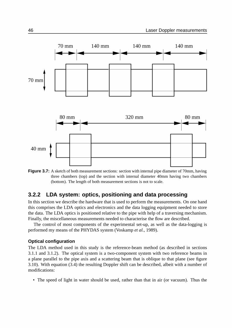
46 Laser Doppler measurements
320 mm80 mm 80 mm
140 mm 140 mm
70 mm
140 mm70 mm
40 mm
Figure 3.7: A sketch of both measurement sections: section with internal pipe diameter of 70mm, havingthree chambers (top) and the section with internal diameter 40mm having two chambers(bottom). The length of both measurement sections is not to scale.
3.2.2 LDA system: optics, positioning and data processingIn this section we describe the hardware that is used to perform the measurements. On one handthis comprises the LDA optics and electronics and the data logging equipment needed to storethe data. The LDA optics is positioned relative to the pipe with help of a traversing mechanism.Finally, the miscellaneous measurements needed to characterise the flow are described.
The control of most components of the experimental set-up, as well as the data-logging isperformed my means of the PHYDAS system (Voskamp et al., 1989).
Optical configurationThe LDA method used in this study is the reference-beam method (as described in sections3.1.1 and 3.1.2). The optical system is a two-component system with two reference beams ina plane parallel to the pipe axis and a scattering beam that is oblique to that plane (see figure3.10). With equation (3.4) the resulting Doppler shift can be described, albeit with a number ofmodifications:
• The speed of light in water should be used, rather than that in air (or vacuum). Thus the

3.2 Experimental set-up 47
898989898989898989898989898898989898989898989898989898898989898989898989898989898898989898989898989898989898:9:9:9:9:9:9:9:9:9:9:9:9:9::9:9:9:9:9:9:9:9:9:9:9:9:9::9:9:9:9:9:9:9:9:9:9:9:9:9::9:9:9:9:9:9:9:9:9:9:9:9:9:
;9;9;9;9;9;9;9;9;9;9;9;9;9;9;;9;9;9;9;9;9;9;9;9;9;9;9;9;9;;9;9;9;9;9;9;9;9;9;9;9;9;9;9;;9;9;9;9;9;9;9;9;9;9;9;9;9;9;<9<9<9<9<9<9<9<9<9<9<9<9<9<<9<9<9<9<9<9<9<9<9<9<9<9<9<<9<9<9<9<9<9<9<9<9<9<9<9<9<<9<9<9<9<9<9<9<9<9<9<9<9<9<
=9=9=9=9=9=9=9=9=>9>9>9>9>9>9>9>9>
?9?9?9?9?9?9?9?@9@9@9@9@9@9@9@A9A9A9A9A9AA9A9A9A9A9AA9A9A9A9A9AB9B9B9B9B9BB9B9B9B9B9BB9B9B9B9B9B
C9C9C9C9CC9C9C9C9CC9C9C9C9CD9D9D9D9DD9D9D9D9DD9D9D9D9D
E9E9EE9E9EE9E9EE9E9EF9F9FF9F9FF9F9FF9F9F
G9GG9GG9GG9GG9GH9HH9HH9HH9H I9II9II9II9I
I9IJ9JJ9JJ9JJ9J
K9KK9KK9KK9KL9LL9LL9LL9L M9M9M9M9M9M9M9M9M9M9M9M9MM9M9M9M9M9M9M9M9M9M9M9M9MN9N9N9N9N9N9N9N9N9N9N9N9NN9N9N9N9N9N9N9N9N9N9N9N9N
O9O9O9O9O9O9O9O9O9O9O9O9OO9O9O9O9O9O9O9O9O9O9O9O9OP9P9P9P9P9P9P9P9P9P9P9P9PP9P9P9P9P9P9P9P9P9P9P9P9PQ9Q9QQ9Q9QR9RR9R
S9S9SS9S9ST9TT9T U9UU9UU9UV9VV9VV9V
W9W9WW9W9WX9XX9X
rotatablefixed
A
d
cross−section A−A’
A’
tube connected to location downstream
ab
ce
Figure 3.8: One chamber of the measurement section: side view (left) and view in direction of pipe axis(right). a: transparent film replacing pipe wall; b: brass ring to which film is glued; c: rubber0-ring; d: glass wall (high quality, plan-parallel).
factor 1λ
becomes nw
λ.
• The unit vectors that give the direction of the beams (eeel), as well as the direction of detection(eeed), are different in water than in air. Using Snell’s law, the direction vectors eeel and eeed can betranslated. Since the glass walls of the measurement section are plane parallel, the directionof the beams is identical on both sides of the glass wall.
• When the reference beam and the scattering beam intersect, the direction of detection coin-cides with the direction of the reference beam (see page 40).
This results in:
fD,is = nw(eeei − eees) · uuu
λwith i = 1, 2 (reference beam 1 or 2), s=scattering beam, (3.5)
which can be summarised in matrix notation as:
(fD,1s
fD,2s
)=
(a1,1s a2,1s a3,1s
a1,2s a2,2s a3,2s
) u1
u2
u3
, (3.6)
where the direction 1 is in the direction of the pipe axis, direction 2 is perpendicular to the planethrough the pipe axis and the optical axis and direction 3 is perpendicular to both 1 and 2. Ifthe optics between laser and front lens (the lens in figure 3.10) are well aligned, the coefficients

48 Laser Doppler measurements
0
47.5
40
27.5
17.5
70
17.5
Start of contraction
42.1
25
Figure 3.9: Dimensions of the pipe contraction (sizes are in mm)
S
R1 R2
S
R1 R2
S
R1, R2
lens
Figure 3.10: Configuration of the laser beams, front view (left), side view (right): S denotes the scatter-ing beam and R1 and R2 are the two reference beams.

3.2 Experimental set-up 49
uθu
u 2
r
φψ
Figure 3.11: Relationship between velocity component u2 in LDA coordinate system and uθ and ur incylindrical coordinate system.
a3,1s and a3,2s are about four orders of magnitude smaller than the other coefficients and can thusbe neglected. In that case (3.6) reduces to a set of two equations, with two unknowns (u1 andu2). However, one is not interested in the velocity components defined in the coordinate systemof the LDA optics, but in those in the cylindrical coordinate system of the pipe, i.e. uz, ur anduθ. If the optical axis of the LDA optics passes through the axis of symmetry of the cylindricalcoordinate system, u1 corresponds to uz and u2 to uθ. More generally, the following relationshipcan be given:
u1 = uz (3.7a)
u2 = uθ cos (φ − ψ) + ur sin((φ − ψ) , (3.7b)
where ψ is the inclination of the LDA optics and φ is the inclination of the line through themeasuring volume and pipe axis (see figure 3.11). Relationship (3.7b) holds as well for the meanvelocities. The relationship between covariances in both coordinate systems is given by
u′1u′1 = u′zu′z (3.8a)
u′2u′2 = sin2 (φ − ψ) u′ru′r + sin 2 (φ − ψ) u′ru′θ+ cos2 (φ − ψ) u′
θu′θ
(3.8b)
u′1u′2 = cos (φ − ψ) u′zu′θ+ sin (φ − ψ) u′ru′z (3.8c)
In order to obtain all three mean velocities as well as all six components of the Reynolds stresstensor at a given point in space, the LDA measurements need to be made under three differentangles ψ (two angles would be sufficient to obtain the mean velocity components only). Thesensitivity of ur, uθ, u′ru′z, and u′zu
′θ, to inaccuracies in the tilting angles ψ (see appendix D) is
minimum when ψ equal -45, 0 and 45 degrees. To reduce errors in u′ru′r, u′θu′θ, and u′ru
′θ
due to

50 Laser Doppler measurements
inaccuracies in ψ, the angles should be -60, 0 and 60 degrees. However, the latter combinationis not permitted by the traversing system, and hence tilting angles ψ of -45, 0 and 45 degrees areused (Steenbergen, 1995).
The procedure to obtain mean velocities and Reynolds stresses is the following:
• uzis obtained by averaging the u1 for all three angles;• urand uθcan be computed from the combination of u2 measured for two different angles ψ
(see (3.7b)); with three available angles, three combinations can be made; the three resultingvalues for ur and uθ are averaged;
• u′zu′zis computed as the average of the three available values for u′1u′1;
• from the combination of u′2u′2 for three different angles u′ru′r, u′ru′θand u′
θu′θcan be computed
(see (3.8c));• with equation (3.8c) u′zu
′θand u′ru′zcan be computed by combining measurements under three
different angles; with three available angles, three different combinations of two angles canbe made; the resulting values for u′ru′zand u′zu
′θare averaged.
Laser and signal processingThe velocity measurements are made using an LDA system of Dantec. The system is basedon the reference beam principle (using forward scattered light). The laser that is used is a 15mW He-Ne laser manufactured by Uniphase. The optics mounted before the laser provide tworeference beams and one scattering beam (see figure 3.10 and 3.12). The scattering beam isshifted in frequency (40MHz) by a Bragg-cell (the Bragg cell is driven by a signal from one ofthe frequency shifters Dantec 55N10). Two different front lenses can be mounted on the optics:one with a focal length ( f ) of 160mm and one with f = 80mm. The beams pass through themeasurement section and the light of the reference beams and the light scattered in the directionof the reference beams is collected by lenses with a focal length of 60mm. Subsequently, it passesthrough a pinhole and finally hits the photo diode (the pinhole is part of the housing of the diodeDantec 55L11). In the shifter the signal from the diode is shifted back by a frequency which isthe sum of the 40MHz pre-shift of the Bragg-cell and a (positive or negative) frequency neededfor an optimal use of the range of the tracker. From the shifter the signal is passed to the Dantectracker 55N21 where the high frequency information is converted to a voltage (between 0 and10 V). The selection of the frequency range of the tracker (out of seven) and the shift frequencyif the shifter (54 available) depends on the Doppler shifts that are generated by the flow. Thechoice of range and shift is always such that measurements in one traverse (−1 < r/R < 1) canbe made with one combination of range and shift.
The analog signal from the tracker is digitised using the parallel sampler (PARSAM) devel-oped by ’Technical Laboratory Automation Group’ at TUE (see Smeets and van Nijmweegen(1993)). Since the PARSAM has an input voltage range of −10V to 10V, a programmable am-plifier3 is used to re-scale the signal from the tracker. The output signal of the lock indicator ofthe tracker is fed directly to the PARSAM. The PARSAM uses a 12bit analog-to-digital converter(ADC). The choice to use a PARSAM in this experiment (rather than a conventional ADC) is
3Built by Jan Niessen.

3.2 Experimental set-up 51
lens
glas wall of box
glas wall of box
sheet
sheetwater
SR1 R2
lens lens
diodediodepinhole pinhole
Figure 3.12: Top view of the path of the laser beams: from front lens of the sending optics, through themeasurement section (glass walls and sheet) toward the diode optics
based on two considerations:
• the PARSAM allows high sampling rates (up to 25 kHz per channel);• two memory buffers (512 kB each) allow continuous operation, so that large amounts of
data can be gathered continuously;
These two latter characteristics are mainly important when information on the temporal structureof the signal is required (such as spectra).
Steenbergen (1995) observed that the response of the trackers used in this study was notlinear and that this non-linearity was mainly linked to the ambient temperature. Therefore thetrackers need to be calibrated daily using a second order polynomial. For this calibration a PhilipsPM5138 function generator is used.
Traversing systemThe traversing system to move around the LDA optics is shown in figure 3.13. The coordinatesof this traversing system are defined as follows:
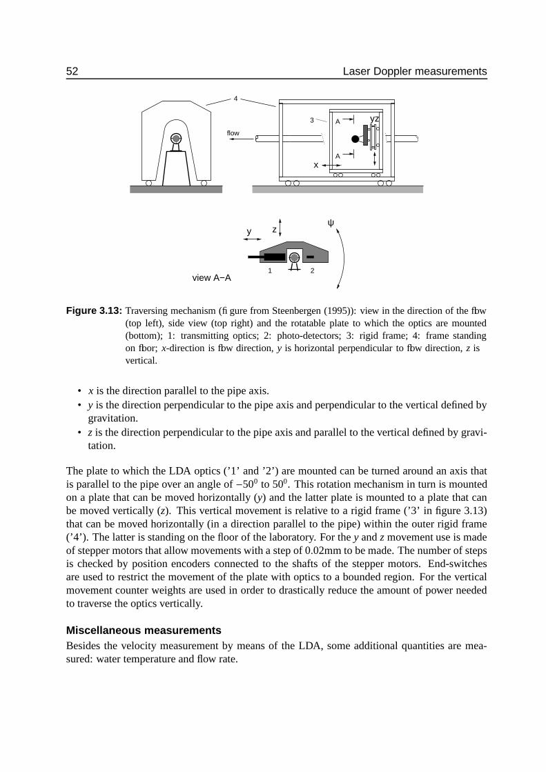
52 Laser Doppler measurements
4
y zψ
x
A
A
view A−A
flow
3
1 2
yz
Figure 3.13: Traversing mechanism (figure from Steenbergen (1995)): view in the direction of the flow(top left), side view (top right) and the rotatable plate to which the optics are mounted(bottom); 1: transmitting optics; 2: photo-detectors; 3: rigid frame; 4: frame standingon floor; x-direction is flow direction, y is horizontal perpendicular to flow direction, z isvertical.
• x is the direction parallel to the pipe axis.• y is the direction perpendicular to the pipe axis and perpendicular to the vertical defined by
gravitation.• z is the direction perpendicular to the pipe axis and parallel to the vertical defined by gravi-
tation.
The plate to which the LDA optics (’1’ and ’2’) are mounted can be turned around an axis thatis parallel to the pipe over an angle of −500 to 500. This rotation mechanism in turn is mountedon a plate that can be moved horizontally (y) and the latter plate is mounted to a plate that canbe moved vertically (z). This vertical movement is relative to a rigid frame (’3’ in figure 3.13)that can be moved horizontally (in a direction parallel to the pipe) within the outer rigid frame(’4’). The latter is standing on the floor of the laboratory. For the y and z movement use is madeof stepper motors that allow movements with a step of 0.02mm to be made. The number of stepsis checked by position encoders connected to the shafts of the stepper motors. End-switchesare used to restrict the movement of the plate with optics to a bounded region. For the verticalmovement counter weights are used in order to drastically reduce the amount of power neededto traverse the optics vertically.
Miscellaneous measurementsBesides the velocity measurement by means of the LDA, some additional quantities are mea-sured: water temperature and flow rate.
3.2 Experimental set-up 53
The water temperature is monitored with the help of a thermal diode of which the signalis converted to a voltage signal with a Laumann temperature display (which also displays thetemperature). The flow rate is measured by an Altometer magnetic flow meter (SC 80 AS),which has a current output proportional to the flow rate. This current is converted to a voltage bypassing the current through a resistor of 470Ω ± 1%. The temperature and flow rate signal aredigitised using a 12 bit ADC.
Incidentally measurements of pressure drop between difference axial positions have beendone. To this purpose pressure taps (with a diameter of 0.5mm) are present in the pipe wall.These taps can be connected to one of the two pressure transducers, Validyne DP15-30 or DP45-16, which have a range of |∆p| ≤ 880 and 35mmH2O, respectively. The signal of these pressuretransducers is passed through an amplifier to a 12 bit ADC.
Alignment and calibrationA number of angles in the geometry of the beams and the flow need to be known or set accurately.Details of these calibrations and alignments can be found in Steenbergen (1995). Here only themain points are given.
• The geometry of the three beams has been determined with a theodolite (for the proceduresee Steenbergen (1995)). For a large part of the experiments the calibration done by Steen-bergen has been used. After a disruption of the alignment by a a careless window-cleanerthis calibration had to be redone.
• The entire pipe (including the measurement section) is made level in the axial direction withan accurate water level.
• The traversing system should be level, both in the directions parallel and perpendicular tothe pipe axes. This is checked with an accurate water level.
• Inclination ψ for measurement section: the (windows of the) measurement section is set tothe correct inclination angle ψ with the help of an accurate water level. For ψ = 0 the waterlevel is place directly on the measurement section, whereas for ψ = ±450 a metal wedge ofexactly 450 is used.
• uz in direction of pipe axis: the optical axis of the LDA system is set perpendicular to thepipe axis: by rotating the LDA system is rotated around its optical axis such that the planethrough the reference beams is vertical; then the traversing system is turned (around its ver-tical axis) until the reflected reference beams (reflected in the window of the measurementsection) fall within the plane of the reference beams themselves.
• Inclination ψ for LDA optics: the optical axis of the LDA system set to the correct inclina-tion ψ horizontal by first turning the LDA system around its optical axis such that the planethrough the reference beams is horizontal; then the plate on which the optics are mounted(see figure 3.13, is turned until the reflected reference beams (reflected in the window of themeasurement section) fall within the plane of the reference beams themselves.
• Rotation of LDA around its optical axis: the LDA system is aligned such that a motion inthe direction of the pipe axis gives a zero vertical velocity according to the LDA. To thisend a transparent plate is used as a scatterer. This plate is slided on top of the measurementsection, parallel to the pipe axes and its velocity in x and z direction is measured with the
54 Laser Doppler measurements
LDA. The LDA optics is rotated around its optical axis until ux and uz given by the LDAindicate that the motion is is purely horizontal within 0.1 degree.
• The coordinate system of the traversing system needs to be tied to the coordinate system ofthe pipe. This is done by measuring (with a telescope which is translated parallel to the pipeaxes) the distance between the intersections of the two reference beams with the pipe wall.This distance is determined three times. Twice with the LDA optics placed such that themeasuring volume is near the pipe axes (the distance between the beam-wall intersection ismeasured at both sides of the pipe: at the pipe wall closest to the laser and at the oppositeside). And once with the LDA optics placed off-axis. From these three measurements, thedistance between the origin of the coordinate system of the traversing system and the pipeaxis can be determined, as well as the pipe diameter. If the latter is within 0.1mm of itsnominal value (either 35mm or 20mm) the alignment is accepted.
The effect of inaccuracies in the above procedures have been analysed by Steenbergen (1995).His results are reproduced in appendix D.
3.3 Measurement strategy
3.3.1 Flow typesThe geometry of the flow domain is a circular pipe containing a contraction; the diameter ofthe pipe upstream of the contraction Du ≡ D = 70mm, whereas downstream the diameter isDd = 40mm.
Two types of flow have been studied: developed turbulent pipe flow and turbulent pipe flowwith swirl. For the measurements without swirl the contraction was situated at 82D downstreamof the swirl generator (which had a vane angle of zero degrees, producing zero swirl) so that inthe inflow of the contraction a fully developed pipe flow could be assumed. For the measurementswith swirl the contraction was placed only 14D downstream of the swirl generator (closer to theswirl generator in order to have a higher swirl number at the entrance of the contraction). In thatcase the angle of the vanes relative to the radial direction was 45 degrees;
Both flows have been studied at two values of ReD (where D is the diameter upstream of thecontraction, i.e. the larger diameter): 2 · 104 and 105, respectively. During the measurements, theReynolds number was required to remain within 1% of its nominal value (where both variationsin flow rate and temperature were taken into account).
For the two types of flow measurements have been performed, at both Reynolds numbers, atsix axial positions. Two of these positions were situated upstream of the contraction (x/D = −5.8and -1.8) and four downstream: x/D = 2.4, 6.9, 11.4 and 25.2. Here the origin of the axialcoordinate is located at the point of the contraction where the radius starts to diminish (indicatedin figure 3.9) and all axial positions have been scaled with the upstream pipe diameter.
At each axial measuring position a number of measurements have been made, as will bedetailed in section 3.3.2 and 3.3.3.

3.3 Measurement strategy 55
Reynoldsnumber
Sampling frequency
D = 40mm D = 70mm
20000 100 50100000 500 200
Table 3.1: Sampling frequency (Hz) for measurements at different bulk Reynolds numbers and in pipesections with different diameters.
3.3.2 Processed dataThe main part of the data gathered, are data to determine the mean velocity and Reynolds stressesat the axial positions mentioned in the previous section and at a large number of radial positions.Data were gathered at 47 radial positions ranging from −0.99R to 0.99R with a higher concen-tration of point near the wall than near the pipe centre. These data are processed before beingstored4. To determine all components of the mean velocity and the Reynolds stress, the measure-ments need to be repeated under three different angles ψ. The traverse along the r-direction (pipecoordinates) was made horizontally (i.e. the y-direction in the coordinate system of the travers-ing system). The sampling frequency is set such that the individual samples (of the continuoustracker signal) are supposed to be independent (see table 3.1). The number of samples is basedon a rough estimate of the required error in variances and covariances and is set to a nominalvalue of 50000.
For each of the radial positions the strategy is as follows:
• The control program moves the measurement volume to the radial position under consider-ation.
• The control program determines the quality of the signal:
– A limited number of samples is taken.– If for less than 75% of these samples the tracker was locked, the number of samples
to be taken is increased in order to retain the originally requested number of samples.If this final number of samples is more than twice the nominal number of samples theposition is skipped for further measurements.
– If for more than 75% of the samples the tracker was locked, the original number ofsamples will be gathered.
• If the position is not skipped because of a lack of locking of the tracker, the measurementswill be made. The quality of the data will be assessed again (the program requires thetracker to have locked for more than 75% of the samples). If the data quality is sufficientthe samples of the velocity signal will be processed and stored to file.
Thus the actual number of samples used for the processing may be between 75% and 100%
4At the moment that this project started, storage capacity was a serious problem, so that storage of all individualsamples seemed not feasible.

56 Laser Doppler measurements
of 50000. Depending on the signal quality data may be not present for some of the 47 radialpositions. Especially the radial positions closest to the wall prove to have a low signal quality.
3.3.3 Raw dataApart from the data that are gathered and processed on-line (previous section), raw velocity dataare gathered and stored for later processing. This is done only for a limited number of radialpositions (because of the limitations in data storage). For each flowtype (swirl or no swirl), ateach axial position, and each Reynolds number, two traverses are made to obtain raw data: ahorizontal traverse to obtain uz and uθ and a vertical traverse for uz and ur. Each traverse consistsof only nine radial positions ranging from r/R = 0 to r/R = 0.97. The sampling frequency dependson the cut-off frequency of the low pass filter of the tracker for the range used 5. The number ofsamples is 2 · 105. Together with the velocity data, also the lock information for both channelsis stored. In the post-processing, samples for which the tracker does not lock are replaced bylinearly interpolated values.
5Only after completion of the experiment it turned out that the filter in the tracker was not very sharp (first orderonly). As a consequence, for some some combinations of range and sampling frequency the sampling frequencywas too low and aliasing occurred. This mainly affects spectra of the measurements at ReD = 2 · 104.
4 Numerical simulation ofturbulence
Three fundamentally different approaches to the numerical modelling of turbulent flows can bedistinguished: Direct Numerical Simulation (DNS), Large Eddy Simulation (LES) and ensembleaveraged modelling1.
In section 2.1.2 it was shown that the ranges of length and time scales present in a turbulentflow depend on the Reynolds number. From (2.6) it can be deduced that even for a moderate(macroscale) Reynolds number of 104 the range of length scales comprises three orders of mag-nitude and the range of time scales one order of magnitude. This large separation between thesmallest and the largest scales forms a challenge to the three major approaches in turbulencemodelling.
In DNS discretized versions of the Navier-Stokes equations (and possibly additional conser-vation equations for scalars) are solved and integrated in time. Due to the large range in scalesone needs a high spatial and temporal resolution. Both increase with Reynolds number. Theinformation one can obtain from a DNS are both instantaneous realisations of the flow and sta-tistical quantities which are obtained from computing statistics in the homogeneous dimensions,be it spatial and/or temporal.
In LES, the problem of the enormous range of scales in a turbulent flow is tackled by spa-tially filtering the governing equations with a filter with characteristic size2l f (see section 4.1.1).In that way the range of length scales is reduced to L/l f . The filtering operation results in ex-tra terms in the governing equations, which describe the influence of the flow at scales smallerthan l f on the flow at scales above the filter size. These terms have the form of the divergenceof stresses and these stresses need to be modelled (see section 4.1.3). These stresses are com-monly —but incorrectly— called ’subgrid-scale stresses’ (SGS-stresses), whereas in principlethey should be named subfilter-scale-stresses. The SGS-stresses provide the communication be-tween the resolved scales (grid scale, or GS) and the dissipation scales. As in the case of DNS,the information one can obtain from LES are instantaneous fields and statistical quantities.
The third approach to the modelling turbulent flows is ensemble averaged modelling. Thisapproach comprises two steps: Reynolds decomposition of all variables in the Navier-Stokesequations (see section 2.1.3) and ensemble averaging of those equations (see (2.9)). These stepsproduce additional terms which contain the so-called Reynolds stresses. In order to close the
1Numerous reviews on these subjects are available: for DNS see Moin and Mahesh (1998), for LES see Reynolds(1989), Lesieur and M etais (1996) or Mason (1994) and concerning ensemble average models see Launder (1990)or Speziale (1989).
2Filtering can both be done in the spatial and the spectral domain. In the latter case a parameterisation is soughtfor the spectral transfer across the wavenumber at which the equations were filtered. From here onward only spatialfiltering will be considered.
57

58 Numerical simulation of turbulence
equations, one needs a model for Reynolds stresses. Various approaches to the modelling of thestresses exist (see Stull, 1988; Wilcox, 1993, for an overview), ranging from first-order closure(Reynolds stresses are estimated from mean quantities), through two-equation models (Spezialeet al., 1992; Speziale, 1987; Wilcox, 1988) to algebraic stress models (Rodi, ????) and second-order closure or Reynolds-stress models (Launder et al., 1975; Launder, 1990).
Section 4.1 describes the principles and the techniques used in Large Eddy Simulation ofturbulent flows. In 4.2 the model used in the present study is described.
4.1 Principles of Large Eddy Simulation4.1.1 Filtering the governing equationsThe equations that are solved in an LES model are filtered versions of the Navier-Stokes equa-tions. Formally, the filtering operation involved in the development of the governing equationsin LES can be defined as:
φ (xxx, t) =∫
φ(xxx′, t)F(xxx − xxx′)dxxx′ (4.1)
where F(xxx − xxx′) is the filtering function and φ is the filtered variable (see Aldama (1990) for adiscussion on filtering)3. The filter function F is non-zero within a distance of the order of l f
from xxx and zero elsewhere. The actual field can be interpreted as a filtered field plus a sub-filterdeviation:
φ = φ + φ∗ (4.2)
Although this expression appears to be similar to the Reynolds decomposition, there are im-portant differences to note. A spatial filter does not necessarily possess all the properties ofan ensemble average (see (A.7)). In particular, the following differences should be mentioned(Reynolds, 1989; Boris et al., 1992):
• Depending on the filter used, the filtering operation may not fulfil the condition that φ = φ .
A spectral sharp cutoff filter does obey φ = φ , whereas a Gaussian filter does not. For
a tophat filter generally φ , φ , unless the filtered variables are defined only at discrete
locations in space and the filter length equals the spatial spacing (see Schumann, 1975b);
• Filtering and differentiation do not commute in general: ∂∂xφ ,
∂∂x φ (where x is either a
space or time coordinate); only when the filter is constant in space and time (e.g. a con-volution filter like equation (4.1)) do filtering and differentiation commute. Non-constantfilters might be useful when the size of the energy containing eddies varies within the flowdomain. Besides, the presence of solid boundaries makes filters vary in space (e.g. van derVen, 1995).
3Note that in (4.1) the filtered variableφφφ is not necessarily a continuous variable in space or time (see Schumann,1975b).
4.1 Principles of Large Eddy Simulation 59
Application of the filtering operation to the continuity equation yields (under the assumptionthat filtering and differentiation commute):
∇∇∇ · uuu = 0 , (4.3)
and the momentum equation becomes:
∂uuu∂t+∇∇∇ · uuu uuu = −1
ρ∇∇∇p +∇∇∇ · νSSS −∇∇∇ · τττ , (4.4)
where τττ is a stress-like tensor resulting from the filtering operation applied to the nonlinearadvection term. In view of the derivation of models for τττ (see section 4.1.3) it is important tonote that this stress is a quantity that varies in space and time. In the sequel, the combination ofequations (4.3) and (4.4) will be called the ’LES-equations’4.
The full expression for this sub-filter scale tensor, τττ, is:
τττ ≡ uuuuuu − uuu uuu =(uuu uuu − uuu uuu
)+
(uuuuuu∗ + uuu∗uuu
)+ uuu∗uuu∗ , (4.5)
where the three terms at the right-hand-side are the Leonard stresses, the cross-stresses and theSGS-stresses, respectively. The SGS tensor τττ contains unknown quantities and needs to be mod-elled (see 4.1.3). It depends on the type of filter used which of these terms are non-zero. Variousapproaches to the treatment of these terms can be followed (Aldama, 1990).
The Leonard terms could be lumped with the advective term and the resulting advective term(∇uuu uuu ) could be obtained by explicit filtering (see e.g. Piomelli and Ferziger, 1988). Alterna-tively the doubly filtered term in the Leonard stress could be approximated with a series expan-sion around uuu uuu (Leonard, 1974; Aldama, 1990; Vreman et al., 1997). In the latter approach oneneeds to take into account that the expansion depends on the filter used, and that the expansionwill result in a third-order term in the filtered Navier-Stokes equation. It will depend on the ac-curacy of the numerical method whether it makes sense to compute this term. Other researchershave just lumped the Leonard term in the parametrisation of the SGS-stress, where it shouldbe kept in mind that the Leonard stresses are dissipative in general (according to the analyticalapproximation by Leonard (1974)).
Although the cross stresses and the SGS-stresses both involve SGS velocities, they are of acompletely different nature. Whereas the SGS-stresses describe the net dissipative effect of theSGS fluctuations on the resolved field, the cross terms describe the random interaction betweenresolved and SGS scale velocity fields (Aldama, 1990). This difference can also be explained interms of the direction in which transfer of energy takes place: either from GS to SGS, or fromSGS to GS. The cross-terms may transfer energy in either direction, both locally (and instanta-neously) and in the mean. On the other hand, the SGS-stresses will –in the mean– transfer energyfrom the GS to the SGS. Locally, however, the direction of energy transfer might be reversed:
4The LES-equations do not contain an independent equation for the pressure. However, this can be constructedby taking the divergence of (4.4) which yields, together with the constraint of incompressibility, a Poisson equationfor the pressure: 1
ρ∇2 p = ∇∇∇ ·
(−∇∇∇ · uuu uuu +∇∇∇ · νSSS −∇∇∇ · τττ
)

60 Numerical simulation of turbulence
backscatter occurs (Kraichnan, 1976; Vreman et al., 1997; Mason and Thomson, 1992). Despitethis difference between the SGS-stress and the cross-terms, the latter are often lumped with theSGS-stresses and parameterised simultaneously by one model.
Before proceeding with the discussion on SGS-stress modelling, it should be noted that gen-erally, SGS-stress models are used to model only the anisotropic part of the SGS-stress tensor.The isotropic part is subtracted from the SGS-stress and added to the dynamic pressure:
τ′τ′τ′ = τττ − 13
tr(τττ)δδδ (4.6)
p′ = p +13
tr(τττ)δδδ , (4.7)
where tr(τττ) is twice the sub-grid scale turbulence kinetic energy, and δδδ is the identity tensor(Kronecker delta).
4.1.2 The relationship between filtering and the SGS-modelAlthough the SGS-stresses appear naturally from the filtering operation, different views existwith respect to the exact link between filtering and SGS-stress (model). In short the debate boilsdown to the question whether the SGS-stress (model) is the consequence of an explicit filteringoperation or is the filtering operation the implicit result of the SGS-stress model used?
• Schumann (1975b) uses the finite volume method to spatially discretise the momentumequations: the equations are integrated over finite subvolumes of the entire flow domain.In terms of the filtering approach, this method could be interpreted as the application of afilter (see (4.1)) that is fixed in space, i.e. fixed to the grid: the tophat filter is non-zeroonly if xxx coincides with the gridpoint of the variable under consideration and xxx′ lies withinthe grid volume. The grid value of a variable represents the mean value averaged over thegrid volume and the SGS-stresses are actual stresses acting on the cell faces, rather thanstresses that exist in the entire cell volume. One of the effects of this way of filtering isthat the Leonard term and the cross-stresses are non-existent in the approach of Schumann.Schumann calls his method the ”volume balance method”.
• Mason and Thomson (1992) state that the form of the filter seen by the resolved motionsis determined by the subgrid model and not by any particular assumed form or type of thefilter. This statement is true as long as there is no explicit reference to the type and size ofthe filter in the governing equations (as in (4.3) and (4.4)). The view of Mason and Thomsonalso implies that a SGS-stress model should not be judged as to how well it represents some–assumed– SGS-stresses. Rather the resulting resolved flow should be evaluated, i.e. theeffect of the SGS-stress model on the resolved scales.
• Piomelli and Ferziger (1988) investigate the relationship between the filter type and theSGS-stress model in an a posteriori test. They show that the resulting flow statistics fora particular SGS-stress model do depend on the filter used (they investigate filters in thespectral domain only) as opposed to the claim of Mason and Thomson (1992), cited above.The difference in view can be attributed to the fact that the filtered Navier-Stokes equationused by Piomelli and Ferziger contains a doubly filtered term: they have a term ∇∇∇uuu uuu on
4.1 Principles of Large Eddy Simulation 61
the left-hand side of (4.4) whereas Mason and Thomson have ∇∇∇uuu uuu 5. This implies that theversion of (4.4) used by Piomelli and Ferziger not only contains a term that depends on theSGS-model, but also on a characteristic of the filter, viz. to what extent does uuu uuu differ fromuuu uuu (see section 4.1.1).
A discussion of some aspects of the relationship between SGS-stress models and spatial discreti-sation, in particular the grid used, can be found in secion 4.1.4.
4.1.3 Subgrid scale-stress modellingSubgrid-scale models are available in roughly three variations, viz. eddy-viscosity models, mod-els based on rate-equations for the SGS-stresses (second-order closure) and models that dependon an extra level of filtering (the dynamic models and scale-similarity models). Since the LESmodel used in the present study uses an eddy-viscosity SGS-stress model, emphasis will be onthis type of SGS-stress parameterisation. The other two types will be discussed at the end of thissection.
Derivation of eddy-viscosity modelsThe origin of eddy-viscosity models lies in the early days of numerical weather prediction (NWP)(Smagorinksy, 1993). As in the case of LES, NWP models needed to assure that the large –resolved– scale motions communicated correctly with the viscous subrange of the spectrum ofatmospheric motion.
The first step is to postulate that the SGS tensor τ′τ′τ′ (the anisotropic part of τ) can be linked tothe rate of strain tensor of the filtered field SSS :
τ′ = −νννt:::SSS , (4.8)
where νννt is in general a fourth-rank tensor6. Based on necessary reflective symmetries and op-tional other types of symmetry the number of independent components of νννt can be reduced.
In order to arrive at the classical Smagorinsky SGS stress model a number of assumptionsneed to be made (Canuto and Cheng, 1997):
• The eddy-viscosity tensor νννt can be replaced by a scalar eddy viscosity νt. This correspondsto the assumption that the SGS-stress tensor and the strain tensor are always aligned.
• Next the assumption of local equilibrium between production (≈ −τ′τ′τ′:::SSS ) 7and dissipation(ε) of SGS-kinetic energy is made:
ε = −τ′τ′τ′:::SSS = νtSSS :::SSS (4.9)
5Piomelli and Ferziger deal with the Leonard term explicitly, whereas Mason and Thomson lump this term with
the other SGS terms. Or, put differently, the former have τττ = uuuuuu − uuu uuu whereas the latter have τττ = uuuuuu − uuu uuu .6Note that the minus in front of νννt depends on both the definition of τττ and the sign in front of the term −∇∇∇ · τττ in
(4.4).7In general, the expression for the production of SGS kinetic energy will depend on the properties of the filter.
For a sharp cut-off filter the expression −τ′τ′τ′:::SSS is an exact representation of the SGS kinetic energy production.
62 Numerical simulation of turbulence
• Finally it is assumed that the separation between GS and SGS motion is located withinthe inertial subrange of homogeneous isotropic turbulence so that the energy spectrum is aKolmogorov spectrum at the GS-SGS separation:
E(k) = αKε2/3k−5/3 , (4.10)
where αK is the Kolmogorov constant. When the filter is characterised by a cutoff wavenum-ber k f =
2πl f
and it is assumed that the Kolmogorov spectrum extends down to k = 0, the
mean square rate of strain (S 2= SSS :::SSS ), and the sub-grid kinetic energy, ES GS , can be
written as:
S 2=
∫ k f
0k2E(k)dk =
32αKε
2/3k4/3f (4.11)
ES GS =
∫ ∞
k f
E(k)dk =32αKε
2/3k−2/3f (4.12)
respectively. From (4.11) it can be deduced that ε ∼(S 2
)3/2and, with (4.9) and (4.11):
νt =
(32αK
)−3/2 (l f
2π
)2
|SSS | = l2 |SSS | (4.13)
where |S | =√
S 2. Since the derivation is based on the assumption of a Kolmogorov typeinertial subrange spectrum (which is based on an ensemble average of flows and not validfor an instantaneous turbulent field), (4.13) is valid only in the ensemble mean. Equation4.12 can be reduced to
ES GS =1
0.27l2 |SSS |2 , (4.14)
by combination of (4.9), and (4.13), and with αK = 1.6
In the early days of the eddy-viscosity model, filtering was done implicitly by the spatialdiscretisation. Thus the filter length was linked to the grid spacing. Since the smallest scaleresolvable on a grid with typical spacing ∆∗ is 2∆∗ (i.e. l f = 2∆∗) it follows from (4.13) that thelink between grid spacing and length scale l is:
l =l f
2π(32αK)−3/4
=∆∗
π(32αK)−3/4 (4.15a)
≡Cs∆∗ , (4.15b)
where Cs is the Smagorinsky constant . The combination of equations (4.13) and (4.15b) is theclassical Smagorinsky model . (4.15b) leads to a theoretical value for C s between 0.17 and 0.28,with αK ranging between 1.6 and 0.8, (see Smagorinksy (1993) for a review). Note that this

4.1 Principles of Large Eddy Simulation 63
derivation for Cs —under the assumptions given— only holds for a sharp spectral cutoff filter 8
and isotropic turbulence. In general Cs will depend on the exact properties of the filter and onthe validity of the assumptions made in the derivation of (4.13). With reference to the type offlow, various values for Cs have been reported, ranging from 0.1 for shear driven turbulence upto 0.23 for isotropic turbulence (see Mason and Callen (1986); Smagorinksy (1993)). Canutoand Cheng (1997) show that the lower value needed in the case of shear flows can be explainedby the invalidity of the assumptions underlying the original derivation of the Smagorinsky model(viz. linear relationship between stress and strain, Kolmogorov type inertial subrange spectrumand local equilibrium of production and dissipation). The reported maximum of 0.23 is less thanthe theoretical upper bound of 0.28.
Apart from the above derivation one could also postulate forms for νt on dimensional grounds.Referring to (4.13) νt is interpreted as the product of a lengthscale squared and an inverse timescale (the strain rate) leading to (4.16a).
νt ∼ L2T −1 , (4.16a)
Or one uses the notion that the SGS-stress is linked to the dissipation of turbulent kinetic energy:νt can be written in terms of the dissipation and a length scale. This can be compared to (2.5)with ν replaced by νt (see also Leslie and Quarini (1979)):
νt ∼ ε13L 4
3 , (4.16b)
A final option is to link the SGS-stress to some velocity scale of the SGS field, for instance—the square root of— the SGS kinetic energy and combined with a length scale, as in (4.16c)(Schumann, 1975b) or a time scale, as in (4.16d) (Horiuti, 1993).
νt ∼ LU , (4.16c)
νt ∼ TU2 . (4.16d)
Modifications to eddy-viscosity modelsGenerally, the derivations of eddy-viscosity SGS-stress models are valid only for isotropic homo-geneous turbulence. Thus anisotropy or inhomogeneity of the flow may invalidate the derivationand will necessitate modifications of the model. In the present context the main points of concernare the effect of the pipe wall and the effect of rotation.
Pipe wall The presence of the pipe wall will both induce inhomogeneity and anisotropy in theflow: mean and fluctuating properties of the flow will become dependent on the distance fromthe wall and fluctuations of the normal-to-the-wall velocity component will be damped relative
8One should be cautious in the translation of results obtained under the assumption of a sharp spectral cutofffilter to other (spatial) filters. Kraichnan (1976) shows a sharp increase of the eddy viscosity as the wavenumberfrom which energy should be drained approaches the wavenumber of the spectral cutoff. On the other hand, resultsfrom Leslie and Quarini (1979) for a Gaussian filter show an eddy viscosity that is mostly constant for wavenumbersbelow the filtering wavenumber and that rapidly decreases as the filter size is approached (see also Mason, 1994).

64 Numerical simulation of turbulence
to the other fluctuations of the other velocity components. Roughly three approaches are used totake into account the presence of a wall:
• The distance to the wall is taken into account explicitly in the length scale in (4.16a). L isadjusted (reduced) close to the wall (van Driest, 1956; Schumann, 1975b).
• Use is made of the sensitivity of some of the properties of the resolved flow field to thepresence of the wall (measures of anisotropy, shear or vorticity for instance). One or moreof the scales used in (4.16) are chosen such that it depends on such a property9.
• Deardorff (1972) suggests to remove the mean shear from the flow field before computingthe strain used in (4.13). In his simulation of a neutrally stratified planetary boundary layerthis resulted in useful simulations with a value of Cs of about 0.2 in the entire domain.
The standard way to take the distance to the wall into account is the first approach, the methodof van Driest (1956):
l = Cs∆∗(1 − exp
(− y+
A+
)), (4.17)
where y+ is the distance from the wall in viscous wall units (y+ = yu∗/ν, with u∗ the frictionvelocity: u∗ =
√τ/ρ) and A+ is a dimensionless constant with an empirical value of 26. The
application of (4.17) only makes sense if both the wall shear stress and the distance to the wallare well-defined.
An example of the second approach is the work of Horiuti (1993) who uses an expression forνt according to (4.16d). His time scale and velocity scale are:
T =ES GS
ε‘, (4.18a)
U =√
ES GS ‘, (4.18b)
where ES GS is the SGS kinetic energy (see equation 4.12). The crucial step made by Horiuti isto replace the velocity scale in (4.18b) by 3
2 of the component of the SGS-stress that is normal tothe wall, here denoted by E⊥S GS
10, which leads to:
νt ∼ ∆∗232
E⊥S GS
|SSS |∼ ∆∗2 3
2
E⊥S GS
ES GS|SSS | (4.19)
This model for νt can be interpreted as the standard Smagorinsky model with a damping functionfor the length scale (compare to (4.17)):
l = Cs∆∗
√32
E⊥S GS
ES GS(4.20)
9The model of Canuto and Cheng (1997) could also be thought to belong to this category, since their modelis also sensitive to both shear and vorticity. Besides, they neither impose a Kolmogorov type inertial subrangespectrum, nor do they impose local equilibrium between production and dissipation.
10In the case of isotropic turbulence 32 E⊥S GS = ES GS .
4.1 Principles of Large Eddy Simulation 65
Yakhot et al. (1990) and Eggels (1994)11 use the fractionE⊥GS
EGSrather than
E⊥SGS
ESGS:
l = Cs∆∗
√32
E⊥GS
EGS(4.21)
This can be justified by the fact that the main contribution to E⊥S GS and ES GS comes from thelargest sub-filter scales12. The anisotropy in the components of the turbulent kinetic energy atthose scales might be comparable to that of the filtered field. Although the approach of Horiuti(1993) —or equivalently Yakhot et al. (1990) and Eggels (1994)— eliminates both the referenceto the wall shear stress (which is implicit in the method of van Driest) and the distance to thewall, the specification of the direction perpendicular to the wall still remains non-trivial exceptfor the case of flow over a flat wall.
Rotation With respect to the influence of rotation on the SGS-stress model two remarks canbe made. Firstly, Ferziger (1993) discusses the applicability of SGS-stress models to flows inwhich extra strains act. He states that as long as the extra strains mainly affect the large-scalephenomena in a flow, the standard SGS-stress models should remain applicable. On the otherhand, the material presented in section 2.2 shows that one of the effects of rotation may be thereduction of dissipation of turbulent kinetic energy. This suggests that the dissipative action ofan eddy-viscosity model should be reduced when mean rotation is present. The results of Canutoand Cheng (1997), who included vorticity in their SGS-model, indeed show a reduction in theeddy-viscosity if the vorticity is non-zero (although in their case vorticity was a result of themean shear, rather than mean rotation).
Other types of SGS-modelsOther types of SGS models used in LES in physical space will be treated only very shortly in thenext sections.
Second-order closure and algebraic stress models As in the case of Reynolds-stress mod-elling, one can derive the rate equations for the elements of the SGS-stress tensor (similar to(2.10)). Some of the terms in such equations are dependent on GS quantities and SGS-stressesand can be computed explicitly. Other terms need parametrisation. Some authors have performedLES with such second-order closure models for the SGS-stresses (Deardorff, 1974). Others havesimplified the differential equations for the SGS-stresses to an algebraic stress model (Schmidt
11Eggels (1994) arrives at a damping factor which would give l = C s∆∗(
32
E⊥SGS
ESGS
)1/4rather than the expression
given in (4.20). The effect of this is that the expression of Eggels gives less damping than that of Horiuti. The originof the difference between the two authors lies in the choice of the scales used to define νt. Whereas Horiuti startsout from (4.16d) (using a time scale and a squared velocity scale), Eggels uses (4.16c) (a length scale and a velocityscale).
12In order to estimate the E⊥GS and EGS one needs some dimension in which the flow is homogeneous: one needsto be able to compute both 〈u⊥′′u⊥′′〉 and 1
2 〈uuu′′ ·uuu′′〉, respectively (where 〈φ〉 signifies the spatial average of variableφ, and φ′′ is the deviation from that spatial average).

66 Numerical simulation of turbulence
and Schumann, 1989). A variant that lies between the second-order closure and eddy-viscositymodels is to use a prognostic equation for the SGS kinetic energy ES GS and to use ES GS in theestimation of νt. According to (4.16c)
√ES GS can then be used as a velocity scale (Deardorff,
1980; Schumann, 1975b).
Structure function model The SGS-viscosity in the Smagorinsky model, as given by (4.13),is a function of the resolved strain rate. However, assuming isotropic turbulence, this may alsobe written in terms of E(k):
νt(xxx) ∼ α−3/2K
(Exxx(k f )
k f
), (4.22)
where Exxx(k) is a local energy spectrum, rather than some global, ensemble averaged, spectrum.This local energy spectrum can be estimated from the second-order structure function of theresolved field, which is given by (for separations r equal to the grid spacing ∆x):
F2(xxx,∆x) = 〈(uuu (xxx) − uuu (xxx + rrr))2〉|rrr|=∆x , (4.23)
where 〈φ〉 signifies the spatial average (in one or more homogeneous directions) of variable φ. F2
can be obtained from the resolved field. For isotropic turbulence, and assuming a Kolmogorovspectrum (in terms of the k-dependence of E(k)) it can be deduced that (4.22) can be approxi-mated as (using the link between F2 and Exxx(k)):
νt ∼ α−3/2K ∆x
√F2(xxx,∆x) (4.24)
For a more elaborate description of the structure function model, see Lesieur and Metais (1996)and Silveira Neto et al. (1993).
Similarity model and mixed model The scale-similarity model (Bardina et al., 1981) modelsthe cross-terms (see (4.5)). The model is based on the assumption that the main interactionbetween sub-filter scale motion and resolved motion takes place between the smallest resolvedscales and the largest sub-filter scales (Piomelli and Ferziger, 1988). Since no information isavailable on the largest sub-filter scales, this information is generated by filtering the velocityfield twice (i.e. uuu ). This yields an estimate for the SGS-stress:
uuuuuu∗ + uuu∗uuu = CB
(uuu uuu − uuu uuu
), (4.25)
where CB is an empirical constant. This model is usually used in simulations where theLeonard terms are calculated explicitly and the standard Smagorinsky model is used for theSGS-stress (uuu∗uuu∗ ). For this total model for τ′ to be Galilean invariant, CB should be 1 (Speziale,1985).
4.1 Principles of Large Eddy Simulation 67
Dynamic model In the dynamic model, information from the resolved scales is used to de-termine the model constant(s) for the SGS-stress model (see for more information: Germano(1992); Piomelli (1993)). Where the SGS-stress tensor is the result of filtering the non-linearterm in the Navier-Stokes equations with a filter of length l f , one could subsequently apply asecond filter with a larger length scale (the test-filter, with length l f 2) to obtain another stress(compare to (4.5)):
TTT ≡ ˜uuuuuu − ˜uuu ˜uuu (4.26)
This TTT is the SGS-stress to be used in the doubly filtered Navier-Stokes equations. The differencebetween TTT and τττ is the contribution of the resolved scales to TTT , i.e. the part of the SGS-stresscarried by motions smaller than the l f 2but larger than l f . This contribution can be obtained fromthe resolved field:
LLL ≡ TTT − τττ
=
(˜uuuuuu − ˜uuu ˜uuu
)−
(˜uuuuuu − ˜uuu uuu
)
= ˜uuu uuu − ˜uuu ˜uuu
(4.27)
If the Smagorinsky model is used for the parametrisation of the SGS-stresses, the anisotropicpart of LLL (i.e. L′L′L′) equals:
L′L′L′ = CMMM = C(l2
f 2|˜SSS |˜SSS − l2
f˜|SSS |SSS
), (4.28)
with C = C2s . Through combination of (4.28) and the anisotropic part of (4.27) a set of equations
for C is obtained in terms of quantities related to the resolved field. One way to obtain one valuefor C is to contract both equations with SSS (Germano, 1992) or MMM (Lilly, 1992). The result isa spatially and temporarily varying field of the model constant C, including negative values forC (i.e. backscatter). In order to prevent numerical instabilities due to excessive backscatter, theresulting C-field is usually filtered or averaged in some way.
Concluding remarks on SGS-stress modelsTo conclude the discussion on SGS-stress models, two remarks are in place.
Firstly, the main function of a SGS-stress model is to drain sufficient turbulent kinetic energyfrom the grid-scale to the sub-grid scale. This drain should take place at wavelengths just aboveor at the filter scale. And the drain of energy should not only be sufficient in magnitude butshould also affect the correct components of the stress tensor.
Secondly, the range of scales resolved in a LES depends on the ratio of the largest scales inthe flow and the smallest resolved scales. The first depends on the domain size, which is in thepresent situation the pipe diameter D. On the other hand, the smallest resolved scales depend onthe filter length. Thus the range of scales could be estimated as NL = D/l f . But given the factthat in the present implementation of the Smagorinsky model l f is directly linked to the grid size∆∗ , a more direct estimate would be NL = D/∆∗.
68 Numerical simulation of turbulence
4.1.4 Solution of the Navier-Stokes equations: some numerical is-sues
Since the equations that govern LES, i.e. the Navier-Stokes equations and the SGS-stress model,cannot be solved analytically the only route that remains is numerical solution of discretizedversions of those equations.
This entails the choice of the location of variables in space and time (grid) and a method toapproximate the different derivatives occurring in the equations under consideration. The dis-cretisation will yield a set of four algebraic equations for the four variables (p′, ur, uθ and uz) atall discrete positions in space and time. To complete this set of algebraic equations appropriateboundary conditions have to be specified. In the three spatial dimensions these comprise bound-ary conditions in both the positive and negative directions, whereas in the time dimension onlyinitial conditions need to be supplied, since there is no information that travels backward in time.
Whereas the discussion of topics concerning spatial and temporal discretisation is beyond thescope of this thesis13 there is one important point with respect to the spatial discretisation thatdoes need to be discussed: the size and shape of the filters used in LES is in most cases closelycoupled to the grid used. Another issue of importance is the specification of boundary conditions(both in space and time), which is not as straightforward as it seems.
SGS-model and spatial discretisationWhen variables are discretized on a regular, rectangular grid the situation is rather simple: thesize of the filter is constant in space. However, there are two reasons to employ a grid that isirregular –or at least not uniform– in space:
• The geometry of the flow may dictate that the grid is distorted in some way as to fit someimposed boundaries. In the present case of flow through an axisymmetric domain this isaccomplished by using cylindrical coordinates. In cylindrical coordinates the tangentialgrid spacing varies proportionally with r. In order for the grid boxes to have nearly thesame aspect ratio –i.e. an isotropic filter– throughout the domain, the radial spacing shouldalso vary with r. However, this would imply that the size of the boxes, and consequentlythe size of the filter would vary wildly through the domain. If on the other hand the size,in terms of volume, would be kept nearly constant, the aspect ratio would vary (see figure4.1).
• The size of eddies one would like to resolve may vary through the flow domain, requiringa varying filtersize. Furthermore, the properties of the flow, such as strong gradients, maydictate a special grid spacing in certain regions of the domain. This also results —whenthe filter size is linked to the grid size– in a varying filter size. For the pipe flow underconsideration this is the case for the radial grid spacing which is reduced in the region nearthe wall, in order to resolve the large shear due to wall friction. In terms of the sketchesgiven in figure 4.1 this will lead to a grid like the one depicted in the right figure.
13The reader is referred to textbooks like Ferziger and Peri c (1996) and Hirsch (1990a) for more information onthe different types of spatial and temporal discretisation.

4.1 Principles of Large Eddy Simulation 69
YZYZYZYZYZYZYYZYZYZYZYZYZYYZYZYZYZYZYZYYZYZYZYZYZYZYYZYZYZYZYZYZYYZYZYZYZYZYZY[Z[Z[Z[Z[Z[[Z[Z[Z[Z[Z[[Z[Z[Z[Z[Z[[Z[Z[Z[Z[Z[[Z[Z[Z[Z[Z[[Z[Z[Z[Z[Z[
\Z\Z\Z\\Z\Z\Z\\Z\Z\Z\]Z]Z]]Z]Z]]Z]Z] ^Z^Z^Z^^Z^Z^Z^^Z^Z^Z^^Z^Z^Z^_Z_Z_Z__Z_Z_Z__Z_Z_Z__Z_Z_Z_
`Z`Z`Z`Z``Z`Z`Z`Z``Z`Z`Z`Z``Z`Z`Z`Z`aZaZaZaZaaZaZaZaZaaZaZaZaZaaZaZaZaZa
Figure 4.1: Sketch of cylindrical coordinates with grid cells of either constant aspect ratio (left) or con-stant volume (right).
The use of cylindrical coordinates with a radial grid spacing decreasing outward has two conse-quences: the filter size varies in space and the filter is anisotropic.
A consequence of the use of a filter that is variable in space is that differentiation and filteringno longer commute, i.e. ∇∇∇φ , ∇∇∇φφφ . This implies that the filtered Navier Stokes equations (4.3)and (4.4) are not exactly valid. However, Ghosal and Moin (1995) show that the error due tothe omission of the extra terms resulting from a non-uniform filter are second-order in the filterwidth. Thus they are of the same order as the discretisation error when a second-order spatialdiscretisation is used. Ghosal and Moin (1995) also showed that the error due to a non-constantfilter size is dissipative. Thus this error can just be added to errors due to the SGS-stress model,which is dissipative as well (at least in the mean). It could even be seen as support for the claimof Mason and Thomson (1992) that the form of the filter as experienced by the resolved field isdetermined by the subgrid model, rather than any assumed form of the filter (see section 4.1.2):the resolved field experiences the dissipation offered by the SGS-stress model. That dissipationmight or might not include the dissipation due to the spatially varying filter size.
The anisotropy of the grid and the consequent anisotropy of the filter has been dealt with bySchumann (1975b), Scotti et al. (1993) and Scotti et al. (1997): the first two authors includedthese effects in terms of a Smagorinsky-like SGS-stress model, whereas the latter focus on thedynamic model. In the ’volume-balancing method’ of Schumann (1975b) (see also section 4.1.2)the SGS-stresses are surface forces, which are proportional to the area of the grid-face on whichthey work. This proportionality is incorporated in the SGS-viscosity, thus Schumann’s viscos-ity becomes anisotropic when the grid is anisotropic. Scotti et al. (1993) on the other hand,translate the anisotropy of the grid into an adaptation of the length scale in the definition of theSGS-viscosity. Thus the viscosity itself remains a scalar. In the analysis of Scotti et al. (1993)the derivation of the Smagorinsky model, given here in section 4.1.3, is redone, taking into ac-count that the filter cut-off wavenumber is not equal in all directions (see (4.11), where k f is the
70 Numerical simulation of turbulence
filtering wavenumber): the smaller the filter length in a given direction, the higher the filteringwavenumber. In the end their analysis yields an expression for the the length scale l in equation(4.15b) that not only depends on the grid spacing ∆∗, but also on the aspect ratio of the grid.
Another consequence of the use of an anisotropic grid may be that the smallest structures thatcan be represented on that grid are anisotropic, solely due to the shape of the grid.
Initial and boundary conditionsSince turbulent flows are highly sensitive to initial conditions one can not expect a numericalsimulation of such a flow to give a faithful representation of the actual temporal development(Lesieur, 1993). Therefore, the initial conditions are immaterial, and in most cases the simulationis started with a random field, where the mean values and the magnitude of the fluctuations arechosen based on prior knowledge of the flow. Starting from this –non-physical– initial fieldthe simulation will –after a number of turbulent time scales– produce a turbulent field that isconsistent with the boundary conditions and external forcings14.
With respect to the specification of spatial boundary conditions three cases can be identified:the boundary may be a solid wall, a fluid with exactly identical properties as the fluid simulated,or a fluid with different properties, i.e. a free surface (the third case is not dealt with here).The specification of solid wall boundary conditions is straightforward in principle. But for thediscretized equations complications will occur when spatial discretisation of order three andhigher are used. Furthermore, when explicit filtering is used in the LES, special care has to betaken near the wall: the filter length should approach zero near the wall.
With respect to boundary conditions within the fluid roughly three options are available:
• When the flow is homogeneous in a given direction, periodic boundary conditions are usu-ally employed. One should ensure that the domain is sufficiently large that the resultingflow at one end of the domain is uncorrelated to the flow half way the domain (the flowat both ends of the domain will be perfectly correlated of course). Numerous examples ofthis approach are available, e.g. Moin and Kim (1982), Eggels et al. (1994) and Nieuwstadtet al. (1993).
• If the flow is not homogeneous in a given direction and there is a net flow in that direction,inflow/outflow boundary conditions can be used. At the inflow plane a turbulent field mustbe specified and at the outflow plane the fluid should be allowed to flow out freely (withoutbackward flow and without reflections). The inflow field may be a field derived from a sepa-rate simulation, or a random field, possibly with appropriate spatial and temporal correlation(e.g. Arnal and Friedrich (1993) and Silveira Neto et al. (1993)).
• In the case of an inhomogeneous direction without a mean flow in that direction, some non-reflecting boundary condition should be devised that allows local inflow and outflow, butimplies a net zero outflow through the boundary. This situation occurs for instance in the
14In case of simulations with unsteady boundary conditions or mean values, e.g. a convective planetary boundarylayer, one would like to reach the state of fully developed turbulence as quickly as possible. The ’start-up’ processmight be helped by using either a turbulent field from a previous simulation or a random field that has been filteredto give at least the correct spatial correlations for the different variables.

4.1 Principles of Large Eddy Simulation 71
vertical direction in the case of flow over a flat plate or the flow in the planetary boundarylayer (Nieuwstadt et al., 1993).
4.1.5 Comparison between LES results and laboratory experimentsIn order to validate the results of an LES, a comparison should be made to results of eithera physical experiment or to another numerical, but more credible, simulation. One practicalobstacle is that it is nearly impossible to exactly match the LES and experiment to which itshould be compared in terms of dimensions and external parameters. Furthermore, due to thechaotic nature of turbulence (extreme sensitivity to initial conditions) LES results and physicalexperiments can be compared only in a statistical sense. A more fundamental problem is thatresults from an LES represent a different view of –ideally– the same experiment. Whereas LESresults provide a –spatially– filtered four-dimensional (space and time) view of the ’true’ velocityand scalar field, point observations in physical experiments only reflect the temporal behaviourof the non-filtered velocity or scalar field. Two approaches are possible to reconcile LES resultsand physical experiments:
• The physical observations can be filtered in a way that is compatible with the filter usedin the LES model. Wyngaard and Peltier (1996) briefly discuss the possibility of spa-tially filtering observations from one point in space (through Taylor’s frozen turbulencehypothesis) to obtain a signal that would be compatible with the resolved scales in an LES.Subsequently, statistical quantities of the LES fields and the filtered observations can becompared.
• The SGS contributions to the statistical quantity under consideration (in particular Reynoldsstresses) have to be added to the resolved part before the LES results can be compared tothe full observations.
In the case that Reynolds stresses are the statistical quantities to be compared, the second ap-proach is followed most often, since the SGS contributions to the Reynolds stresses is available(or can be estimated in a consistent way) from the LES. Since the SGS contribution relies on theSGS-stress model directly, it is good practice to show this contribution separately (apart fromthe sum of resolved stress and SGS-stress). A situation in which one would choose for the firstoption is when spectral quantities (including correlation functions) are considered. Since in anLES the smallest scales present in those quantities are limited to twice the filter scale, it is mostpractical to remove all fluctuations at smaller scales from the results of the physical experiment.
4.1.6 Sources of error in LESIn order to judge the results from a simulation vis-a-vis experimental results, one should havean indication of the error that is inherent to the results of the simulations as well as the errorin the experimental results. For there will always be a difference between the results from thesimulation and the experiment. Only when the ranges in which both results are known to belocated –i.e. the observed value plus and minus the possible error– do not overlap there is reasonto reject the simulation results.

72 Numerical simulation of turbulence
Three fundamentally different sources of error can be identified in relationship to LES re-sults:
• The SGS-stress model is an approximation to the true SGS-stresses. In fact it is usually thisfactor that one aims to test when LES results are validated against observations. Thereforeit is not necessary to take this error into account into the error estimate.
• The equations that are actually solved in an LES model are the discretized approximationsto the true, continuous equations. (Kravchenko and Moin, 1997) discuss both aliasing errorsand truncation errors, of which the latter are most important for the type of discretisationused in the present work. A general approach to determine the errors due to discretisation isto repeat a given simulation for different grid sizes. Mason (1994) suggests a range of fourorders of magnitude in the grid size. The ultimate aim is to show grid-independence of thesolution at a given resolution. A disadvantage of this method in the context of LES is that theinfluence of the SGS-stress model also decreases upon grid-refinement15, and so does theabsolute value of the contribution of the SGS-model to the total error. Furthermore, the orderof the discretisation method used does give information on the rate at which discretisationerrors decrease upon refinement of the grid. However, it does not give information on theactual size of the error.
• Since the turbulence simulated with an LES is a stochastic process, the statistical quantitiesderived from LES results are also stochastic variables. Therefore there will be a differ-ence between the LES-derived statistical quantities and their ensemble average values (orexpected values). The estimation of this difference is rather straightforward and frequentlyapplied to experimental data (Lumley and Panofsky, 1964; Lenschow et al., 1994) but hardlyever used in the context of LES results. Michels (personal communication) developed ex-tended the work of Lenschow et al. (1994) for turbulent data with an arbitrary number ofdimensions (incl. 4-D LES data). A summary of her method is given in section A.3.
4.2 An LES model for pipe flow with swirl and axial strainIn section 4.1 various aspects of large eddy simulation were discussed. The present section dealswith the specific implementation of an LES model as used for this study of the combined effectof swirl and axial strain on turbulent pipe flow.
The model used in this study is based on the model developed by Eggels (1994) and Pourquie(1994) with some modifications by B.J. Boersma (1994-1995) at TUD. The characteristics of theoriginal model can be summarised as:
• Coordinate system: cylindrical coordinates with grid refinement in the radial direction(smaller grid cells near the wall);
• Spatial discretisation: finite volume method;• Temporal discretisation: second-order Adams-Bashforth method, except for advection and
diffusion terms that contain derivatives in the tangential direction. The latter are approxi-mated with the implicit second-order Crank-Nicholson method.
15Unless the filter size is not varied with the grid size (see Mason and Callen (1986)).

4.2 An LES model for pipe flow with swirl and axial strain 73
r = f( ζ) ρ
ζ) ρr = f(
= constant
ρ
bcbcbbcbcbbcbcbbcbcbbcbcbbcbcbbcbcbbcbcbbcbcbbcbcbdcddcddcddcddcddcddcddcddcddcdececeececeececeececeececeececeececeececeececeecece
fcffcffcffcffcffcffcffcffcffcf
Physical coordinate system Transformed coordinate system
ζ
u −velocity
z
u −velocity
r = constant
rz
z
Figure 4.2: Relationship between the (cylindrical) physical coordinate system and the transformed sys-tem.
• Sub-grid scale stresses: Smagorinsky model. Wall-damping of the sub-grid scale stresses isprovided with the Van Driest damping function.
• Boundary conditions: periodic in tangential and axial direction. In the radial direction theboundary conditions at the wall are Dirichlet conditions for all velocity components andVon Neumann conditions for ur and p′.
All lengths in the model are made dimensionless by the pipe diameter D, whereas the velocitiesand pressure are non-dimensionalised by the friction velocity u∗.
In order to simulate the flow through a pipe contraction, as is required in this study, modifica-tions need to be made to the original model on all points mentioned above. The implementationof the new model is discussed in the next sections:
• The coordinate system needs to be modified, leading to new governing equations in thatsystem (section 4.2.1);
• The spatial discretisation needs to be adjusted to the new coordinate system (section 4.2.2);• The temporal discretisation needs to be changed, as well as the method to solve the equation
for the pressure (section 4.2.3).• The subgrid-stress model needs to adapted to the new geometry (section 4.2.4);• The new geomtery requires different boundary conditions (section 4.2.5).
A sketch (to scale) of the domain of the model as related to the configuration in the laboratoryexperiment can be found in figure 1.5 on page 5. The computational domain is also shown infigure 4.4.
4.2.1 Coordinate systemThe original model is based on the Navier-Stokes equations in cylindrical coordinates (see B.1).In order to make simulations of the flow through a contraction, the cylindrical coordinate system
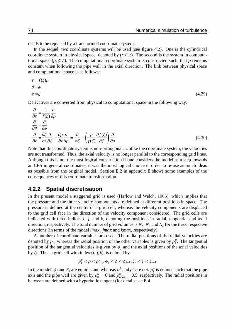
74 Numerical simulation of turbulence
needs to be replaced by a transformed coordinate system.In the sequel, two coordinate systems will be used (see figure 4.2). One is the cylindrical
coordinate system in physical space, denoted by (r, θ, z). The second is the system in computa-tional space (ρ, φ, ζ). The computational coordinate system is constructed such, that ρ remainsconstant when following the pipe wall in the axial direction. The link between physical spaceand computational space is as follows:
r = f (ζ)ρ
θ =φ
z =ζ (4.29)
Derivatives are converted from physical to computational space in the following way:
∂
∂r=
1f (ζ)
∂
∂ρ
∂
∂θ=∂
∂φ
∂
∂z=∂ζ
∂z∂
∂ζ+∂ρ
∂z∂
∂ρ=
∂
∂ζ−
(ρ
f (ζ)∂ f (ζ)∂ζ
)∂
∂ρ(4.30)
Note that this coordinate system is non-orthogonal. Unlike the coordinate system, the velocitiesare not transformed. Thus, the axial velocity is no longer parallel to the corresponding grid lines.Although this is not the most logical construction if one considers the model as a step towardsan LES in general coordinates, it was the most logical choice in order to re-use as much ideasas possible from the original model. Section E.2 in appendix E shows some examples of theconsequences of this coordinate transformation.
4.2.2 Spatial discretisationIn the present model a staggered grid is used (Harlow and Welch, 1965), which implies thatthe pressure and the three velocity components are defined at different positions in space. Thepressure is defined at the centre of a grid cell, whereas the velocity components are displacedto the grid cell face in the direction of the velocity component considered. The grid cells areindicated with three indices i, j, and k, denoting the positions in radial, tangential and axialdirection, respectively. The total number of grid volumes is Nr, Nθ and Nz for the three respectivedirections (in terms of the model imax, jmax and kmax, respectively).
A number of coordinate variables are used. The radial positions of the radial velocities aredenoted by ρu
i , whereas the radial position of the other variables is given by ρpi . The tangential
position of the tangential velocities is given by φ j and the axial positions of the axial velocitiesby ζk. Thus a grid cell with index (i, j, k), is defined by
ρui < ρ < ρ
ui−1, φ j < φ < φ j−1, ζk < ζ < ζk−1
In the model, φ j and ζk are equidistant, whereas ρpi and ρu
i are not. ρui is defined such that the pipe
axis and the pipe wall are given by ρu0 = 0 and ρu
imax = 0.5, respectively. The radial positions inbetween are defined with a hyperbolic tangent (for details see E.4.

4.2 An LES model for pipe flow with swirl and axial strain 75
For the factor f that describes the axial variation of the radius, two variables are employed.f wk gives the value of f at ζ = ζk, whereas f p
k gives f at the pressure point (ζ = ζk − 12dζ;
f pk =
12
(f wk + f w
k−1
)). Furthermore, the axial derivative of f at the same positions is used, denoted
by d f wk and d f p
k , respectively.The equations are discretized by integrating them over the relevant grid volume, of which the
edges depend on the variable under consideration. This method is similar to the ”volume balancemethod” of Schumann (1975b), though his SGS-stress model is quite different. Whenever valuesof variables are needed at positions where they are not defined, interpolation with a mid-pointrule is used (for a detailed discussion on the accuracy see Eggels (1994) and Pourquie (1994)).As an example of the discretisation procedure, the derivation of the discretized divergence isgiven in appendix E.
4.2.3 Temporal discretisation and pressure solutionFor the time discretisation a fractional step method is used (Ferziger and Peric, 1996; Kim andMoin, 1985, see). This implies that each time step is split into two steps. The first step (fromtime level tn to an intermediate –undefined– level t∗) comprises the tendencies due to advectionand diffusion terms only (see equation 2.2). The second step (from time level t∗ to tn+1) solelyincludes the tendency due to the pressure gradient term.
First stepFor the time discretisation of most terms the second order Adams-Bashforth method is used (seee.g. Ferziger and Peric (1996)):
uuu n+1 ≈ uuu n+
dt2
(3∂uuu n
∂t− ∂uuu n−1
∂t
)(4.31)
where the superscript n denotes the moment in time, and ∂uuu n/∂t is the estimate of the timederivative, based on variables at time step n. These time derivatives only include the advectionand diffusion terms. In order to study both the stability of the time discretisation one needs anexpression of the maximum permissible time step.
From Schumann (1975a) it can be concluded that the maximum permissible time step is16
dtmax ≤ βmρ
|u i, j,kr |
f pk (ρp
i+1 − ρpi )+ mφ
|u i, j,kθ|
f pk ρ
pi dφ+ mζ
|u i, j,kz |
dζ+
2(ν + νt)
mρ
1
f pk
2dρi2+ mφ
1
f pk
2ρ
pi
2dφ2+ mζ
1
dζ2
−1
(4.32)
where mρ, mφ and mζ are indicators whether the term should be included (m = 1) or not (m = 0).If all terms in the advection and diffusion terms are treated explicitly, mρ, mφ and mζ are all equal
16More general expressions for the stability limits of different time stepping methods can be found in Wesseling(1996).

76 Numerical simulation of turbulence
to 1. β is a safety factor to account for non-linear effects (in the current study it appears that βneeds to be set to 0.35, which is lower than the values reported by Schumann (1975a) and Eggels(1994) for rectangular and cylindrical grids, respectively.).
Two regions can be distinguished in which the time step can be severely limited:
• Downstream of a contraction the shear near the wall can be significant, resulting in a largeνt; in combination with the small values of dρp
i or dρui due to grid refinement near the wall.
This results in a severe reduction of the time step for the diffusion terms with derivatives inthe radial direction;
• Near the pipe centre, f pk ρ
pi dφ becomes very small.
In order to circumvent these time step limitations, it was decided to treat some terms implic-itly:
• in the region 14 imax < i < imax the diffusion and advection terms containing derivatives in
the radial direction are treated implicitly;• in the region 0 < i ≤ 1
4 imax the diffusion and advection terms containing derivatives in thetangential direction are treated implicitly;
These terms are advanced in time with the Crank-Nicholson method, which can be sum-marised as:
uuu n+1 ≈ uuu n+
dt2
(∂uuu n
∂t+∂uuu n+1
∂t
)(4.33)
The Crank-Nicholson method is unconditionally stable, so the terms no longer pose a stabilitylimit on the time step. For the inner region (4.32) applies with nρ = 1, nφ = 0 and nζ = 1 whereasthe time step limit for the outer region follows from (4.32) with nρ = 0, nφ = 1 and nζ = 1.
The final product of the first step is an intermediate field uuu ∗ computed from the tendenciesdue to diffusion (diff) and advection (adv):
uuu ∗ = uuu n+ dt
(32
diffnexpl −
12
diffn−1expl +
12
diffnimpl +
12
diff∗impl +32
advnexpl −
12
advn−1expl
)(4.34)
Second stepIn an incompressible flow the pressure is not a dynamic variable but is completely coupled tothe velocity field. This coupling is such that the pressure field makes the velocity field obey thecontinuity equation.
In this second step, the pressure field is determined such that application of the pressuregradient term to the velocity field at time level t∗ will yield a divergence-free velocity field attime level tn+1. Thus the step:
uuu n+1 − uuu ∗
dt= −∇∇∇ p′ (4.35)
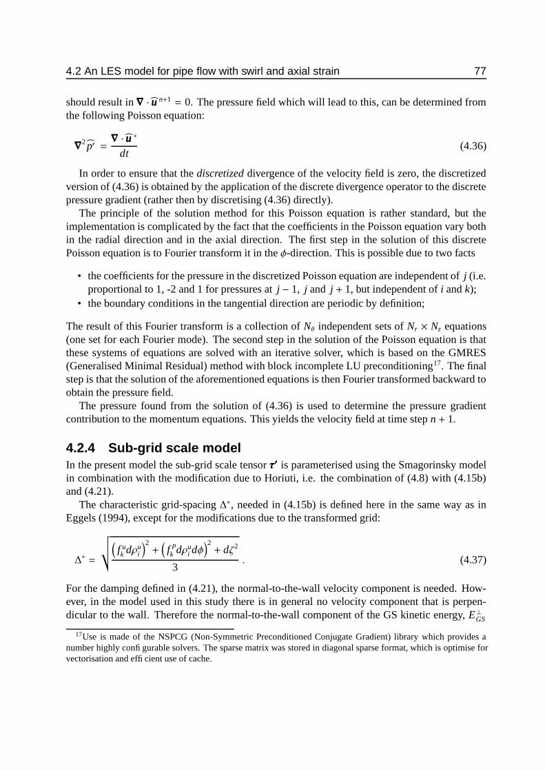
4.2 An LES model for pipe flow with swirl and axial strain 77
should result in ∇∇∇ · uuu n+1= 0. The pressure field which will lead to this, can be determined from
the following Poisson equation:
∇∇∇2 p′ =∇∇∇ · uuu ∗
dt(4.36)
In order to ensure that the discretized divergence of the velocity field is zero, the discretizedversion of (4.36) is obtained by the application of the discrete divergence operator to the discretepressure gradient (rather then by discretising (4.36) directly).
The principle of the solution method for this Poisson equation is rather standard, but theimplementation is complicated by the fact that the coefficients in the Poisson equation vary bothin the radial direction and in the axial direction. The first step in the solution of this discretePoisson equation is to Fourier transform it in the φ-direction. This is possible due to two facts
• the coefficients for the pressure in the discretized Poisson equation are independent of j (i.e.proportional to 1, -2 and 1 for pressures at j − 1, j and j + 1, but independent of i and k);
• the boundary conditions in the tangential direction are periodic by definition;
The result of this Fourier transform is a collection of Nθ independent sets of Nr × Nz equations(one set for each Fourier mode). The second step in the solution of the Poisson equation is thatthese systems of equations are solved with an iterative solver, which is based on the GMRES(Generalised Minimal Residual) method with block incomplete LU preconditioning17. The finalstep is that the solution of the aforementioned equations is then Fourier transformed backward toobtain the pressure field.
The pressure found from the solution of (4.36) is used to determine the pressure gradientcontribution to the momentum equations. This yields the velocity field at time step n + 1.
4.2.4 Sub-grid scale modelIn the present model the sub-grid scale tensor τ′τ′τ′ is parameterised using the Smagorinsky modelin combination with the modification due to Horiuti, i.e. the combination of (4.8) with (4.15b)and (4.21).
The characteristic grid-spacing ∆∗, needed in (4.15b) is defined here in the same way as inEggels (1994), except for the modifications due to the transformed grid:
∆∗=
√√(f uk dρu
i
)2+
(f pk dρu
i dφ)2+ dζ2
3. (4.37)
For the damping defined in (4.21), the normal-to-the-wall velocity component is needed. How-ever, in the model used in this study there is in general no velocity component that is perpen-dicular to the wall. Therefore the normal-to-the-wall component of the GS kinetic energy, E⊥GS
17Use is made of the NSPCG (Non-Symmetric Preconditioned Conjugate Gradient) library which provides anumber highly configurable solvers. The sparse matrix was stored in diagonal sparse format, which is optimise forvectorisation and efficient use of cache.

78 Numerical simulation of turbulence
ruu
ru
zu u
ρ = constant
Figure 4.3: Construction of velocity components u⊥ and u‖. The orientation of these components de-pends on the local slope of the ρ = constant lines. The components u⊥ and u‖ are constructedat the pressure point in the staggered grid, by linear combination of the ur and uz velocitycomponents.
should be constructed from the other velocity components. This is done by determining threenew velocity components that are perpendicular and parallel to the local lines of equal ρ (seefigure 4.3). Thus the orientation of these new velocity components changes with position. Thesevelocity components are constructed by linear combination of the ur, uθ and uz velocity compo-nents. One of the attractive properties of defining u⊥ in this way that the u⊥ is continuous acrossthe centreline: there the component u⊥ is perpendicular to the pipe axis.
To estimate the GS kinetic energy, as well as the contribution of the normal-to-the wall veloc-ity component to it, means and fluctuations of the velocity components need to be defined. Tothis end, averaging takes place in the tangential direction, being the only homogeneous directionin this particular flow (see footnote 12).
4.2.5 Boundary conditionsThe boundary conditions in the tangential direction are straightforward, since these are periodicby definition. Therefore, the discussion will focus on the boundary conditions in radial and axialdirection.
Boundary conditions in radial directionBoundary conditions for u r: At the pipe axis ur has a grid value (on a gridbox face withzero surface area). This value is obtained by interpolation between u 1, j,k
r and u 1, j+ jmax/2,kr . For
a discussion about this procedure the reader is referred to Eggels (1994). At the pipe wall (i =

4.2 An LES model for pipe flow with swirl and axial strain 79
imax) the radial velocity is zero. For the ur-point, beyond the wall (at i = imax+1) the divergenceis used. Since ∂
∂φuθ = 0 and ∂
∂ζuz = 0 at the pipe wall, the remaining terms in the divergence are:
1ρ f (ζ)
∂ρu r
∂ρ− ρ
f (ζ)∂ f (ζ)∂ζ
∂u z
∂ρ= 0 (4.38)
Details on the implementation can be found in appendix E.3.1.
Boundary conditions for u θ: At the pipe axis, the boundary condition is obtained from thegrid point for i = 1 at the opposite side of the pipe axis. Minus the value of u θ at that point istaken as the value for u θ at i = 0. For the boundary condition at the pipe wall a no-slip conditionis used: uθ = 0.
Boundary conditions for uz: The boundary conditions for u z are similar to those of u θ: At thepipe axis: the value is derived from a mirror point at the opposite side of the axis. At the pipewall a no-slip boundary condition is applied.
Boundary conditions for p′: For the pressure p′, the boundary conditions are as follows.Both at the pipe axis and the pipe wall a Von Neumann boundary condition is used for thepressure. At the pipe axis ∂p′/∂n (where n is the direction normal to the pipe axis) can simply beimplemented. However, at the wall boundary, the situation is more complicated. Since the linebetween the pressure points on either side of the pipe wall is not at right angles with that pipewall, the pressure gradient normal to the wall –which should be zero– has to be approximated.This is done by interpolating the pressure both inside and outside the pipe wall to points that arelocate on a line that is perpendicular to the pipe wall. Details can be found in E.3.2.
Boundary conditions in axial direction: inflowBoundary conditions for velocities: At the inflow plane prescribed values for the velocitiesare used. The inflow boundary conditions for the velocities are generated with a separate LESmodel with periodic boundary conditions and parallel walls. The discretisation and the SGS-model in that model are identical to those in the model with the contraction. The forcing of theaxial velocity is done with a pressure gradient that is constant in space and time, and which hasa non-dimensional magnitude of 4. This value can be derived from the following force balance(see (2.12c)):
0 =π
4D2∆p + (πDL) ρu∗
2 , (4.39)
where L is the domain length and ∆p is the pressure drop over the total domain (here, ρ isdensity). This leads to a dimensionless pressure drop D/
(ρu∗2
)∂∂z p = 4.
For the simulations with swirl, the non-zero tangential velocity has to be introduced somehow.Two options are discussed here. The two methods have in common that the exact shape of theforcing depends on the swirling flow one desires to simulate.

80 Numerical simulation of turbulence
One possibility is to apply an artificial force that depends on the difference between the actualmean tangential velocity and the uθ-profile of the flow to be simulated. This method has beenused by van Haarlem (1995). The artificial force is an integrator of the deviation of the simulatedu θ-profile from the target profile, and is formulated as:
f n+1θ = f n
θ + α ((uθ)meas − 〈uθ〉n) (4.40)
where n is an indicator of the time step, 〈u θ〉 is the tangential velocity averaged in the homoge-neous directions (i.e. axial and tangential) and (uθ)meas is the measured mean tangential velocity.van Haarlem (1995) reports that the relaxation factor α should be set to 1. Since fθ accumulatesdeviations of 〈u θ〉 from (uθ)meas, the risk exists that the forcing is non-zero, while (uθ)meas − 〈uθ〉equals zero, which in turn might lead to oscillations around the target u θ. To prevent this, in thefirst stage of the simulation (uθ)meas is increased gradually to its final value:
f n+1θ = f n
θ + α
(tn+1
tr(uθ)meas − 〈u θ〉n
)(4.41)
where tr is the time in which the target profile is relaxed from zero to its final value. Thus 4.40holds for t ≥ tr and 4.41 for t < tr. The disadvantage of this forcing is that it is not constantin time and care has to taken to prevent oscillations. On the other hand this forcing will yield acorrect uθ-profile.
Another possibility is to introduce an artificial force that is constant in time as well as inthe axial direction, but varies in the radial direction. Integrated over the pipe cross section, thetangential forcing fθ will act to oppose the tangential wall shear stress τθ,wall. In fact, this fθ actsas if it is a tangential pressure gradient. From (2.12b) it can be deduced, under the assumptionsof stationarity, axisymmetry, axial homogeneity and ur = 0 (and without making the equationsdimensionless):
0 = fθ +1r∂rτrθ
∂r+τrθ
r
= fθ +1r2
∂
∂r
(r2τrθ
)
= fθ −1r2
∂
∂r
(r2u′ru
′θ− r2ν
∂uθ∂r− uθ
r
). (4.42)
This forcing fθ will be dependent on the radial coordinate and it can be derived from measure-ments of turbulent stresses and the mean uθ velocity profile. The advantage of this forcing methodis that the forcing is constant in time and that the u′ru
′θ-profile will be correct in the simulation.
There is no guarantee, however, that the uθ-profile will be correct.
Boundary conditions for pressure: At the inflow plane a zero-gradient boundary condition isused.
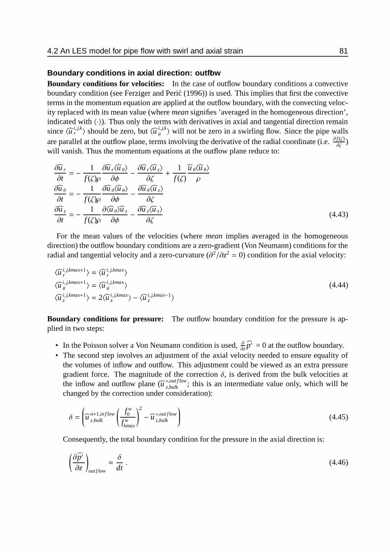
4.2 An LES model for pipe flow with swirl and axial strain 81
Boundary conditions in axial direction: outflowBoundary conditions for velocities: In the case of outflow boundary conditions a convectiveboundary condition (see Ferziger and Peric (1996)) is used. This implies that first the convectiveterms in the momentum equation are applied at the outflow boundary, with the convecting veloc-ity replaced with its mean value (where mean signifies ’averaged in the homogeneous direction’,indicated with 〈·〉). Thus only the terms with derivatives in axial and tangential direction remainsince 〈u i, j,k
r 〉 should be zero, but 〈u i, j,kθ〉 will not be zero in a swirling flow. Since the pipe walls
are parallel at the outflow plane, terms involving the derivative of the radial coordinate (i.e. ∂ f (ζ)∂ζ
)will vanish. Thus the momentum equations at the outflow plane reduce to:
∂u r
∂t= − 1
f (ζ)ρ∂u r〈u θ〉∂φ
− ∂u r 〈u z〉∂ζ
+1
f (ζ)u θ〈u θ〉ρ
∂u θ
∂t= − 1
f (ζ)ρ∂u θ〈u θ〉∂φ
− ∂u θ〈u z〉∂ζ
∂u z
∂t= − 1
f (ζ)ρ∂〈u θ〉u z
∂φ− ∂u z〈u z〉
∂ζ(4.43)
For the mean values of the velocities (where mean implies averaged in the homogeneousdirection) the outflow boundary conditions are a zero-gradient (Von Neumann) conditions for theradial and tangential velocity and a zero-curvature (∂2/∂z2
= 0) condition for the axial velocity:
〈u i, j,kmax+1r 〉 = 〈u i, j,kmax
r 〉〈u i, j,kmax+1
θ〉 = 〈u i, j,kmax
θ〉
〈u i, j,kmax+1z 〉 = 2〈u i, j,kmax
z 〉 − 〈u i, j,kmax−1z 〉
(4.44)
Boundary conditions for pressure: The outflow boundary condition for the pressure is ap-plied in two steps:
• In the Poisson solver a Von Neumann condition is used, ∂∂z p′ = 0 at the outflow boundary.
• The second step involves an adjustment of the axial velocity needed to ensure equality ofthe volumes of inflow and outflow. This adjustment could be viewed as an extra pressuregradient force. The magnitude of the correction δ, is derived from the bulk velocities atthe inflow and outflow plane (u ∗,out f low
z,bulk ; this is an intermediate value only, which will bechanged by the correction under consideration):
δ =
u n+1,in f lowz,bulk
(f w0
f wkmax
)2
− u ∗,out f lowz,bulk
(4.45)
Consequently, the total boundary condition for the pressure in the axial direction is:
(∂p′
∂z
)
out f low
=δ
dt. (4.46)

82 Numerical simulation of turbulence
ghghghghghghghghghghghghghghghghghgghghghghghghghghghghghghghghghghghgghghghghghghghghghghghghghghghghghgghghghghghghghghghghghghghghghghghgghghghghghghghghghghghghghghghghghgghghghghghghghghghghghghghghghghghgghghghghghghghghghghghghghghghghghgihihihihihihihihihihihihihihihihihiihihihihihihihihihihihihihihihihihiihihihihihihihihihihihihihihihihihiihihihihihihihihihihihihihihihihihiihihihihihihihihihihihihihihihihihiihihihihihihihihihihihihihihihihihiihihihihihihihihihihihihihihihihihi jhjhjhjjhjhjhjjhjhjhjjhjhjhjjhjhjhjjhjhjhjjhjhjhjjhjhjhjjhjhjhjjhjhjhjjhjhjhjjhjhjhjjhjhjhjjhjhjhjjhjhjhjjhjhjhjkhkhkhkkhkhkhkkhkhkhkkhkhkhkkhkhkhkkhkhkhkkhkhkhkkhkhkhkkhkhkhkkhkhkhkkhkhkhkkhkhkhkkhkhkhkkhkhkhkkhkhkhkkhkhkhk
1.86
flow
1
0.57
1
Figure 4.4: Domain of the LES model with contraction (all sizes are in expressed in upstream pipediameters D.
4.3 Strategy of the simulationsThe aim of this study is to simulate the same flow situation as described in section 3.3 of whichthe measurement results will be presented in chapter 5. Due to the limitations of LES, onlythe flow at ReD = 20000 will be simulated. Since the LES model is formulated in terms ofRe with u∗ rather than Ubulk, the relationship between u∗ and Ubulk needs to be known. For adeveloped pipe flow the relationship between u∗and Ubulk only depends on the Reynolds number:
u∗/Ubulk = 0.199 · Re− 1
8D (Blasius, 1908). From this it follows that Re should be approximately
1150. For a swirling flow u∗/Ubulk will be different, but also for the simulations of swirling pipeflow Re = 1150 will be used.
Two domain sizes need to be defined: for the straight pipe model and for the model includinga contraction. For the straight pipe model a length of 5 will be used (since the length is non-dimensionalised with D, this corresponds with 5D in the physical experiment). According toEggels (1994) this should be sufficient –at least for the non-swirling flow– not to be botheredby artificial axial correlation due to the periodic boundary conditions. For the model of thecontraction the total domain has a length of 6, where the start of the contraction (i.e. the pointwhere the diameter starts to decrease) is located at 1.8 downstream of the inflow plane. Thiscorresponds to the laboratory experiment where the measurement section just upstream of thecontraction is located 1.8D upstream of the start of the contraction as well. The domain of thecontraction model is shown in figure 4.4
The spatial resolution to be used is shown in tables 4.1, together with some other key param-eters. The relatively high resolution in the tangential direction has been chosen based on trialruns (see appendix F). It turns out that for a good representation of the uθ-fluctuations in thenear wall region a high resolution in the tangential direction is needed. Given the streaky natureof turbulence in the near wall region, where elongated vortices are moving in the streamwisedirection, one would expect the spatial extent of ur-fluctuations and uθ-fluctuations to be compa-rable. Hence for a faithful representation one would need a comparable resolution in the r and θdirection (see also the remarks in section 4.1.4). The total number of grid points is based on thetest for grid-independence given in appendix F.

4.3 Strategy of the simulations 83
quantity straight pipe contraction
Nr 50 50Nθ 224 224Nz 224 269Cs 0.1 0.1Re = u∗D
ν1150 1150 (upstream)
constant for non-uniform grid(see E.4 page 194)
0.97 0.97
Table 4.1: Overview of the most important parameters for simulations per model: the straight pipe modelused to generate inflow and the contraction model to do the actual simulation.

84 Numerical simulation of turbulence

5 Analysis of laboratorymeasurements
In this chapter the results of the laboratory experiments will be presented and discussed. Theexperiments have been performed with the set-up as presented in section 3.2. This chapter isorganised as follows: in section 5.1 the data on the mean flow and Reynolds stresses are pre-sented (both for the swirling and non-swirling flow) with only a minimum of interpretation andexplanation. Further analyses of these data are made in section 5.2. These analyses comprisean attempt to explain and interpret the observations presented in 5.1. Points of attention are theaxial development of the swirl number, the development of the stress anisotropy tensor and acomparison to predictions following from RDT. Subsequently, in section 5.3.1 quantities derivedfrom the time series such as spectra and correlation functions are presented.
5.1 Mean flow and Reynolds stresses: dataThis section will be devoted primarily to the mere presentation of experimental data on mean flowand Reynolds stresses. Explanations of observed phenomena, further analysis and comparisonto other experiments is postponed to the next section.
5.1.1 A note on the presentation of dataBefore unveiling the data, first some remarks on the presentation should be made:
• The data are presented for all six axial positions in one figure, with the vertical axis shiftedupward for each position (the downstream direction in the experiment is upward in thefigure, see for example figure 5.1). The axial positions to which the data refer are notedin the centre column, between the two sets of graphs. These axial positions z have beenscaled with the pipe diameter upstream of the contraction. As discussed in section 3.2 theorigin of the axial coordinate lies at the start of the transition from the large diameter pipeto the smaller diameter (see figure 3.9 at page 48). Thus axial positions upstream of thecontraction are indicated by a negative value for z/D.
• The mean velocities are normalised with the bulk velocity Ubulk based on the local pipediameter, whereas the turbulent stresses are normalised with Ubulk
2. The radial position isnormalised with the local pipe radius, so that the data always cover the range −1 < r/R <
1. These normalisations have been chosen to optimally use the space within the graphs.Besides, the local bulk velocity bears some relationship to the local wall shear stress, so thatthe scaling with Ubulk can easily be converted to a scaling with u∗ 1.
1For a developed pipe flow the relationship between u ∗and Ubulk only depends on the Reynolds number:
85
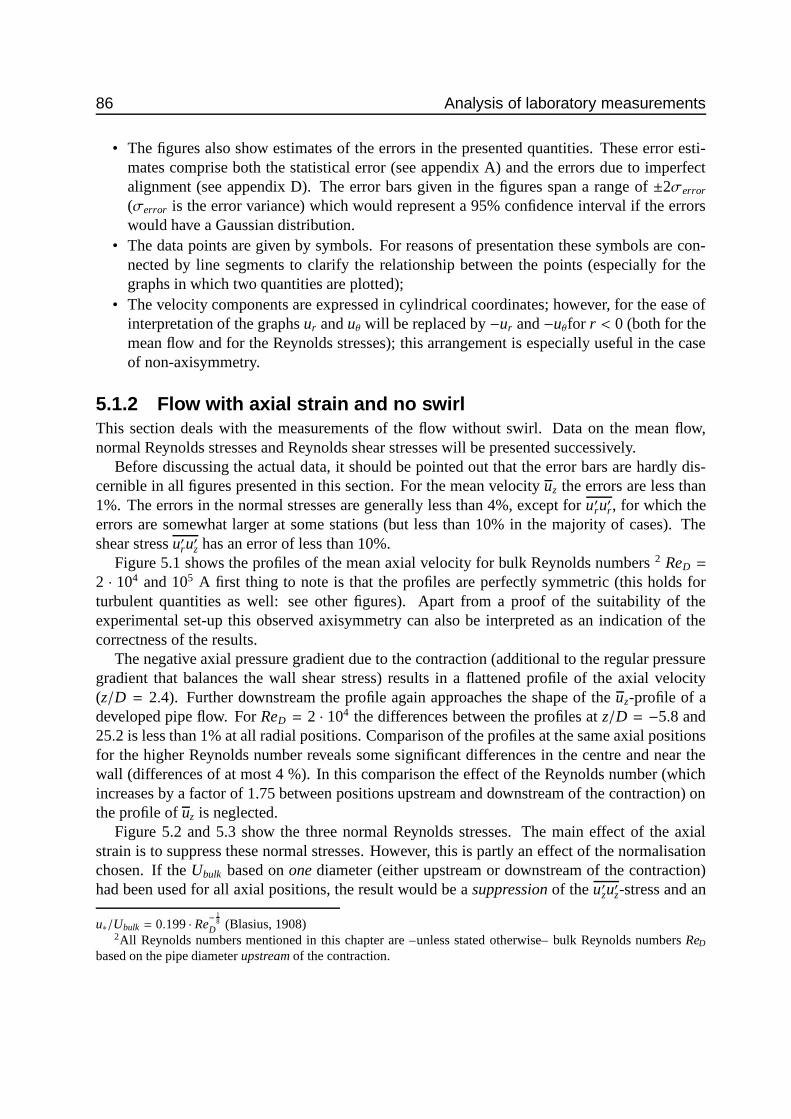
86 Analysis of laboratory measurements
• The figures also show estimates of the errors in the presented quantities. These error esti-mates comprise both the statistical error (see appendix A) and the errors due to imperfectalignment (see appendix D). The error bars given in the figures span a range of ±2σerror
(σerror is the error variance) which would represent a 95% confidence interval if the errorswould have a Gaussian distribution.
• The data points are given by symbols. For reasons of presentation these symbols are con-nected by line segments to clarify the relationship between the points (especially for thegraphs in which two quantities are plotted);
• The velocity components are expressed in cylindrical coordinates; however, for the ease ofinterpretation of the graphs ur and uθ will be replaced by −ur and −uθfor r < 0 (both for themean flow and for the Reynolds stresses); this arrangement is especially useful in the caseof non-axisymmetry.
5.1.2 Flow with axial strain and no swirlThis section deals with the measurements of the flow without swirl. Data on the mean flow,normal Reynolds stresses and Reynolds shear stresses will be presented successively.
Before discussing the actual data, it should be pointed out that the error bars are hardly dis-cernible in all figures presented in this section. For the mean velocity uz the errors are less than1%. The errors in the normal stresses are generally less than 4%, except for u′ru′r, for which theerrors are somewhat larger at some stations (but less than 10% in the majority of cases). Theshear stress u′ru′z has an error of less than 10%.
Figure 5.1 shows the profiles of the mean axial velocity for bulk Reynolds numbers 2 ReD =
2 · 104 and 105 A first thing to note is that the profiles are perfectly symmetric (this holds forturbulent quantities as well: see other figures). Apart from a proof of the suitability of theexperimental set-up this observed axisymmetry can also be interpreted as an indication of thecorrectness of the results.
The negative axial pressure gradient due to the contraction (additional to the regular pressuregradient that balances the wall shear stress) results in a flattened profile of the axial velocity(z/D = 2.4). Further downstream the profile again approaches the shape of the uz-profile of adeveloped pipe flow. For ReD = 2 · 104 the differences between the profiles at z/D = −5.8 and25.2 is less than 1% at all radial positions. Comparison of the profiles at the same axial positionsfor the higher Reynolds number reveals some significant differences in the centre and near thewall (differences of at most 4 %). In this comparison the effect of the Reynolds number (whichincreases by a factor of 1.75 between positions upstream and downstream of the contraction) onthe profile of uz is neglected.
Figure 5.2 and 5.3 show the three normal Reynolds stresses. The main effect of the axialstrain is to suppress these normal stresses. However, this is partly an effect of the normalisationchosen. If the Ubulk based on one diameter (either upstream or downstream of the contraction)had been used for all axial positions, the result would be a suppression of the u′zu′z-stress and an
u∗/Ubulk = 0.199 · Re− 1
8D (Blasius, 1908)
2All Reynolds numbers mentioned in this chapter are –unless stated otherwise– bulk Reynolds numbers ReD
based on the pipe diameter upstream of the contraction.

5.1 Mean flow and Reynolds stresses: data 87
z/D
uz
1.31.21.1
10.90.80.70.6
1.31.21.1
10.90.80.70.6
1.31.21.1
10.90.80.70.6
1.31.21.1
10.9
0.80.70.6
1.31.21.1
10.90.80.70.6
r/R
u z
10.50-0.5-1
1.31.21.1
10.90.80.70.6
25.2
11.4
6.9
2.4
contraction
−1.8
−5.8
uz
1.31.21.1
10.90.80.70.6
1.31.21.1
10.90.80.70.6
1.31.21.1
10.90.80.70.6
1.31.21.1
10.9
0.80.70.6
1.31.21.1
10.90.80.70.6
r/R
u z
10.50-0.5-1
1.31.21.1
10.90.80.70.6
Figure 5.1: Mean velocity uz/Ubulk at ReD = 2 · 104 (left) and ReD = 100000 (right): no swirl

88 Analysis of laboratory measurements
z/Duz′uz′
0.025
0.02
0.015
0.01
0.005
0
0.025
0.02
0.015
0.01
0.005
0
0.025
0.02
0.015
0.01
0.005
0
0.025
0.02
0.015
0.01
0.005
0
0.025
0.02
0.015
0.01
0.005
0
r/R
u z′u
z′
10.50-0.5-1
0.025
0.02
0.015
0.01
0.005
0
25.2
11.4
6.9
2.4
contraction
−1.8
−5.8
uz′uz′
0.025
0.02
0.015
0.01
0.005
0
0.025
0.02
0.015
0.01
0.005
0
0.025
0.02
0.015
0.01
0.005
0
0.025
0.02
0.015
0.01
0.005
0
0.025
0.02
0.015
0.01
0.005
0
r/R
u z′u
z′
10.50-0.5-1
0.025
0.02
0.015
0.01
0.005
0
Figure 5.2: Normal stress u′zu′z/Ubulk2 at ReD = 2 · 104 (left) and ReD = 100000 (right): no swirl

5.1 Mean flow and Reynolds stresses: data 89
z/Duθ′uθ′ur′ur′
0.0080.0070.0060.0050.0040.0030.0020.0010
0.0080.0070.0060.0050.0040.0030.0020.001
0
0.0080.0070.0060.0050.0040.0030.0020.0010
0.0080.0070.0060.0050.0040.0030.0020.001
0
0.0080.0070.0060.0050.0040.0030.0020.0010
r/R
u r′u
r′u θ′u
θ′
10.50-0.5-1
0.0080.0070.0060.0050.0040.0030.0020.001
0
25.2
11.4
6.9
2.4
contraction
−1.8
−5.8
uθ′uθ′ur′ur′
0.0080.0070.0060.0050.0040.0030.0020.0010
0.0080.0070.0060.0050.0040.0030.0020.001
0
0.0080.0070.0060.0050.0040.0030.0020.0010
0.0080.0070.0060.0050.0040.0030.0020.001
0
0.0080.0070.0060.0050.0040.0030.0020.0010
r/R
u r′u
r′u θ′u
θ′
10.50-0.5-1
0.0080.0070.0060.0050.0040.0030.0020.001
0
Figure 5.3: Normal stresses u′ru′r/Ubulk2 and u′
θu′θ/Ubulk
2 at ReD = 2 ·104 (left) and ReD = 100000 (right): no swirl
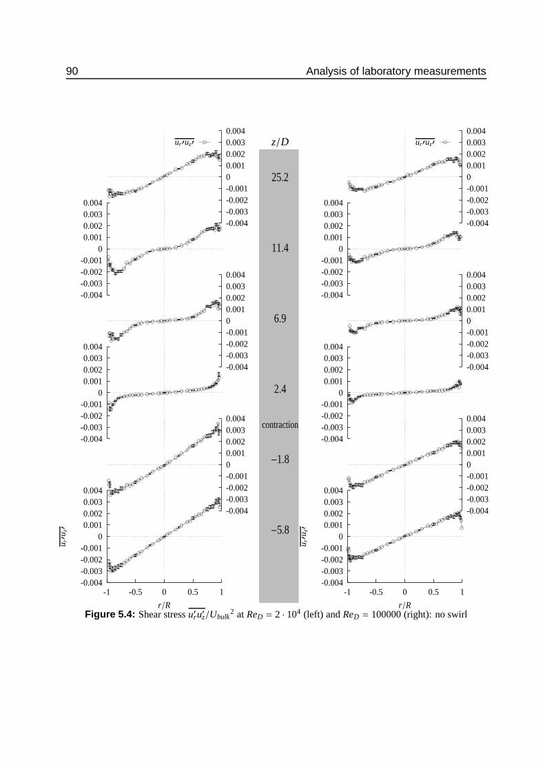
90 Analysis of laboratory measurements
z/Dur′uz′0.0040.0030.0020.0010-0.001-0.002-0.003-0.004
0.0040.0030.0020.001
0-0.001-0.002-0.003-0.004
0.0040.0030.0020.0010-0.001-0.002-0.003-0.004
0.0040.0030.0020.001
0-0.001-0.002-0.003-0.004
0.0040.0030.0020.0010-0.001-0.002-0.003-0.004
r/R
u r′u
z′
10.50-0.5-1
0.0040.0030.0020.001
0-0.001-0.002-0.003-0.004
25.2
11.4
6.9
2.4
contraction
−1.8
−5.8
ur′uz′0.0040.0030.0020.0010-0.001-0.002-0.003-0.004
0.0040.0030.0020.001
0-0.001-0.002-0.003-0.004
0.0040.0030.0020.0010-0.001-0.002-0.003-0.004
0.0040.0030.0020.001
0-0.001-0.002-0.003-0.004
0.0040.0030.0020.0010-0.001-0.002-0.003-0.004
r/R
u r′u
z′
10.50-0.5-1
0.0040.0030.0020.001
0-0.001-0.002-0.003-0.004
Figure 5.4: Shear stress u′ru′z/Ubulk2 at ReD = 2 · 104 (left) and ReD = 100000 (right): no swirl
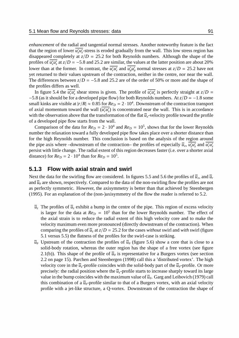
5.1 Mean flow and Reynolds stresses: data 91
enhancement of the radial and tangential normal stresses. Another noteworthy feature is the factthat the region of lower u′zu′z-stress is eroded gradually from the wall. This low stress region hasdisappeared completely at z/D = 25.2 for both Reynolds numbers. Although the shape of theprofiles of u′zu′z at z/D = −5.8 and 25.2 are similar, the values at the latter position are about 20%lower than at the former. In contrast, the u′ru′r and u′
θu′θ
normal stresses at z/D = 25.2 have notyet returned to their values upstream of the contraction, neither in the centre, nor near the wall.The differences between z/D = −5.8 and 25.2 are of the order of 50% or more and the shape ofthe profiles differs as well.
In figure 5.4 the u′ru′z shear stress is given. The profile of u′ru′z is perfectly straight at z/D =−5.8 (as it should be for a developed pipe flow) for both Reynolds numbers. At z/D = −1.8 somesmall kinks are visible at |r/R| ≈ 0.85 for ReD = 2 · 104. Downstream of the contraction transportof axial momentum toward the wall (u′ru′z) is concentrated near the wall. This is in accordancewith the observation above that the transformation of the flat uz-velocity profile toward the profileof a developed pipe flow starts from the wall.
Comparison of the data for ReD = 2 · 104 and ReD = 105, shows that for the lower Reynoldsnumber the relaxation toward a fully developed pipe flow takes place over a shorter distance thanfor the high Reynolds number. This conclusion is based on the analysis of the region aroundthe pipe axis where –downstream of the contraction– the profiles of especially uz, u′zu′z and u′ru′zpersist with little change. The radial extent of this region decreases faster (i.e. over a shorter axialdistance) for ReD = 2 · 104 than for ReD = 105.
5.1.3 Flow with axial strain and swirlNext the data for the swirling flow are considered. In figures 5.5 and 5.6 the profiles of uz, and ur
and uθ are shown, respectively. Compared to the data of the non-swirling flow the profiles are notas perfectly symmetric. However, the axisymmetry is better than that achieved by Steenbergen(1995). For an explanation of the (non-)axisymmetry of the flow the reader is referred to 5.2.
uz The profiles of uz exhibit a bump in the centre of the pipe. This region of excess velocityis larger for the data at ReD = 105 than for the lower Reynolds number. The effect ofthe axial strain is to reduce the radial extent of this high velocity core and to make thevelocity maximum even more pronounced (directly downstream of the contraction). Whencomparing the profiles of uz at z/D = 25.2 for the cases without swirl and with swirl (figure5.1 versus 5.5) the flatness of the profiles for the swirl-case is striking.
uθ Upstream of the contraction the profiles of uθ (figure 5.6) show a core that is close to asolid-body rotation, whereas the outer region has the shape of a free vortex (see figure2.1(b)). This shape of the profile of uθ is representative for a Burgers vortex (see section2.2 on page 15). Parchen and Steenbergen (1998) call this a ’distributed vortex’. The highvelocity core in the uz-profile coincides with the solid-body part of the uθ-profile. Or moreprecisely: the radial position where the uz-profile starts to increase sharply toward its largevalue in the bump coincides with the maximum value of uθ. Garg and Leibovich (1979) callthis combination of a uθ-profile similar to that of a Burgers vortex, with an axial velocityprofile with a jet-like structure, a Q-vortex. Downstream of the contraction the shape of

92 Analysis of laboratory measurements
z/D
uz
1.31.21.1
10.9
0.80.70.6
1.31.21.1
10.9
0.80.70.6
1.31.21.1
10.9
0.80.70.6
1.31.21.1
10.9
0.80.70.6
1.31.21.1
10.9
0.80.70.6
r/R
u z
10.50-0.5-1
1.31.21.1
10.9
0.80.70.6
25.2
11.4
6.9
2.4
contraction
−1.8
−5.8
uz
1.31.21.1
10.9
0.80.70.6
1.31.21.1
10.9
0.80.70.6
1.31.21.1
10.9
0.80.70.6
1.31.21.1
10.9
0.80.70.6
1.31.21.1
10.9
0.80.70.6
r/R
u z
10.50-0.5-1
1.31.21.1
10.9
0.80.70.6
Figure 5.5: Mean velocity uz/Ubulk at ReD = 2 · 104 (left) and ReD = 105 (right): with swirl
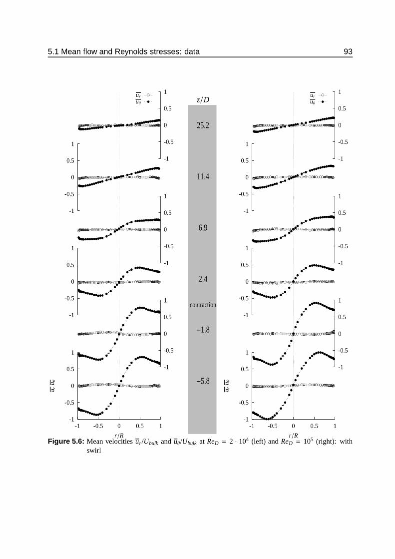
5.1 Mean flow and Reynolds stresses: data 93
z/Duθur
1
0.5
0
-0.5
-1
1
0.5
0
-0.5
-1
1
0.5
0
-0.5
-1
1
0.5
0
-0.5
-1
1
0.5
0
-0.5
-1
r/R
u ru θ
10.50-0.5-1
1
0.5
0
-0.5
-1
25.2
11.4
6.9
2.4
contraction
−1.8
−5.8
uθur
1
0.5
0
-0.5
-1
1
0.5
0
-0.5
-1
1
0.5
0
-0.5
-1
1
0.5
0
-0.5
-1
1
0.5
0
-0.5
-1
r/R
u ru θ
10.50-0.5-1
1
0.5
0
-0.5
-1
Figure 5.6: Mean velocities ur/Ubulk and uθ/Ubulk at ReD = 2 · 104 (left) and ReD = 105 (right): withswirl
94 Analysis of laboratory measurements
z/Duz′uz′0.0450.040.0350.030.0250.020.0150.010.0050
0.0450.04
0.0350.03
0.0250.02
0.0150.01
0.0050
0.0450.040.0350.030.0250.020.0150.010.0050
0.0450.04
0.0350.03
0.0250.02
0.0150.01
0.0050
0.0450.040.0350.030.0250.020.0150.010.0050
r/R
u z′u
z′
10.50-0.5-1
0.0450.04
0.0350.03
0.0250.02
0.0150.01
0.0050
25.2
11.4
6.9
2.4
contraction
−1.8
−5.8
uz′uz′0.0450.040.0350.030.0250.020.0150.010.0050
0.0450.04
0.0350.03
0.0250.02
0.0150.01
0.0050
0.0450.040.0350.030.0250.020.0150.010.0050
0.0450.04
0.0350.03
0.0250.02
0.0150.01
0.0050
0.0450.040.0350.030.0250.020.0150.010.0050
r/R
u z′u
z′
10.50-0.5-1
0.0450.04
0.0350.03
0.0250.02
0.0150.01
0.0050
Figure 5.7: Normal stress u′zu′z/Ubulk2 at ReD = 2 · 104 (left) and ReD = 105 (right): with swirl

5.1 Mean flow and Reynolds stresses: data 95
z/Duθ′uθ′ur′ur′
0.050.0450.040.0350.030.0250.020.0150.010.0050
0.050.045
0.040.035
0.030.025
0.020.015
0.010.005
0
0.050.0450.040.0350.030.0250.020.0150.010.0050
0.050.045
0.040.035
0.030.025
0.020.015
0.010.005
0
0.050.0450.040.0350.030.0250.020.0150.010.0050
r/R
u r′u
r′u θ′u
θ′
10.50-0.5-1
0.050.045
0.040.035
0.030.025
0.020.015
0.010.005
0
25.2
11.4
6.9
2.4
contraction
−1.8
−5.8
uθ′uθ′ur′ur′
0.050.0450.040.0350.030.0250.020.0150.010.0050
0.050.045
0.040.035
0.030.025
0.020.015
0.010.005
0
0.050.0450.040.0350.030.0250.020.0150.010.0050
0.050.045
0.040.035
0.030.025
0.020.015
0.010.005
0
0.050.0450.040.0350.030.0250.020.0150.010.0050
r/R
u r′u
r′u θ′u
θ′
10.50-0.5-1
0.050.045
0.040.035
0.030.025
0.020.015
0.010.005
0
Figure 5.8: Normal stresses u′ru′r/Ubulk2 and u′
θu′θ/Ubulk
2 at ReD = 2 · 104 (left) and ReD = 105 (right):with swirl
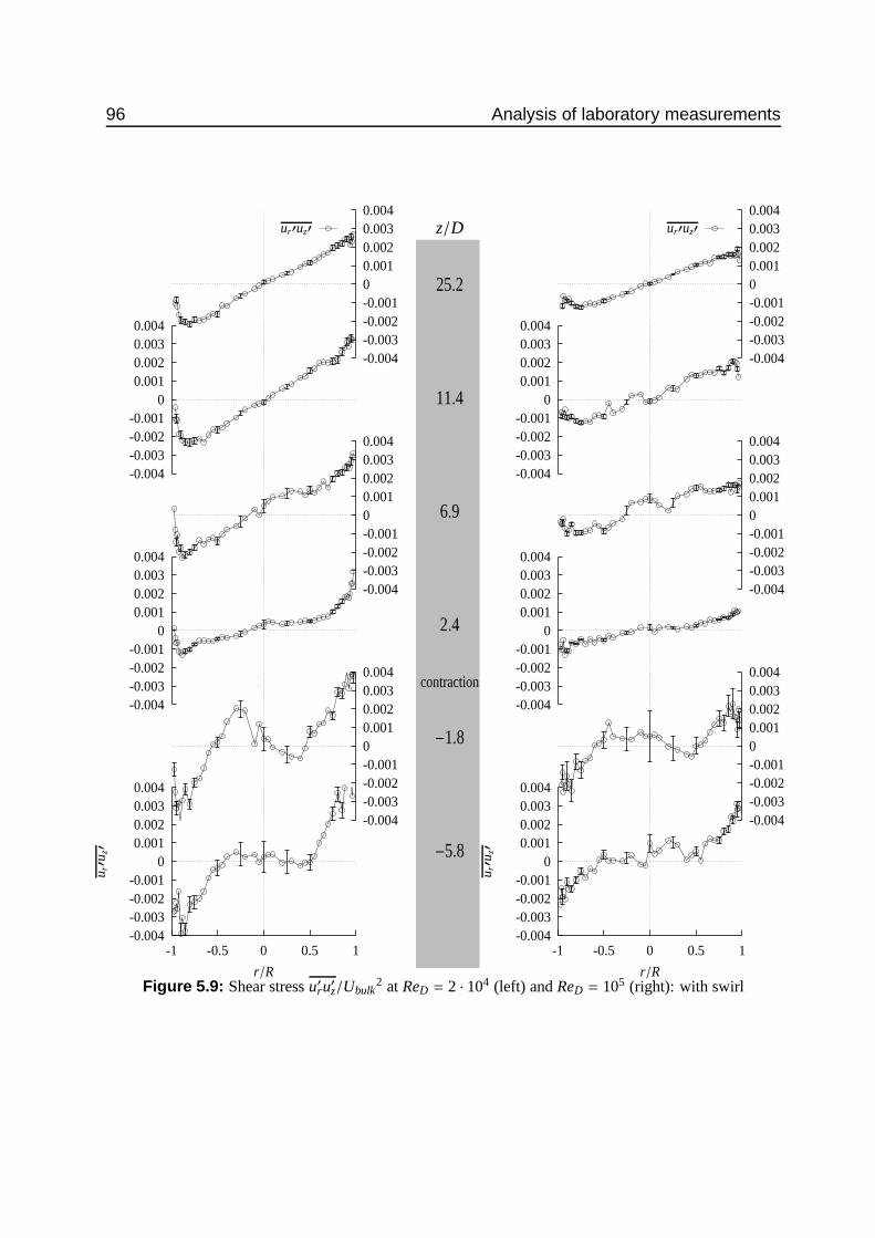
96 Analysis of laboratory measurements
z/Dur′uz′0.0040.0030.0020.0010-0.001-0.002-0.003-0.004
0.0040.0030.0020.001
0-0.001-0.002-0.003-0.004
0.0040.0030.0020.0010-0.001-0.002-0.003-0.004
0.0040.0030.0020.001
0-0.001-0.002-0.003-0.004
0.0040.0030.0020.0010-0.001-0.002-0.003-0.004
r/R
u r′u
z′
10.50-0.5-1
0.0040.0030.0020.001
0-0.001-0.002-0.003-0.004
25.2
11.4
6.9
2.4
contraction
−1.8
−5.8
ur′uz′0.0040.0030.0020.0010-0.001-0.002-0.003-0.004
0.0040.0030.0020.001
0-0.001-0.002-0.003-0.004
0.0040.0030.0020.0010-0.001-0.002-0.003-0.004
0.0040.0030.0020.001
0-0.001-0.002-0.003-0.004
0.0040.0030.0020.0010-0.001-0.002-0.003-0.004
r/R
u r′u
z′
10.50-0.5-1
0.0040.0030.0020.001
0-0.001-0.002-0.003-0.004
Figure 5.9: Shear stress u′ru′z/Ubulk2 at ReD = 2 · 104 (left) and ReD = 105 (right): with swirl

5.1 Mean flow and Reynolds stresses: data 97
z/Dur′uθ′uz′uθ′
0.006
0.004
0.002
0
-0.002
-0.004
-0.006
0.006
0.004
0.002
0
-0.002
-0.004
-0.006
0.006
0.004
0.002
0
-0.002
-0.004
-0.006
0.006
0.004
0.002
0
-0.002
-0.004
-0.006
0.006
0.004
0.002
0
-0.002
-0.004
-0.006
r/R
u z′u
θ′u
r′uθ′
10.50-0.5-1
0.006
0.004
0.002
0
-0.002
-0.004
-0.006
25.2
11.4
6.9
2.4
contraction
−1.8
−5.8
ur′uθ′uz′uθ′
0.006
0.004
0.002
0
-0.002
-0.004
-0.006
0.006
0.004
0.002
0
-0.002
-0.004
-0.006
0.006
0.004
0.002
0
-0.002
-0.004
-0.006
0.006
0.004
0.002
0
-0.002
-0.004
-0.006
0.006
0.004
0.002
0
-0.002
-0.004
-0.006
r/R
u z′u
θ′u
r′uθ′
10.50-0.5-1
0.006
0.004
0.002
0
-0.002
-0.004
-0.006
Figure 5.10: Shear stresses u′zu′θ/Ubulk2 and u′ru′θ/Ubulk
2 at ReD = 2 · 104 (left) and ReD = 105 (right):with swirl

98 Analysis of laboratory measurements
the uθ-profile does not change much, but the maximum value shifts slightly toward the pipecentre. At z/D = 11.4 the local maximum in uθ has disappeared and so has the bump inuz. The fact that the value of uθ is lowered on passage through the contraction is perhapscounter-intuitive. However, one should remember that —apart from some swirl decay–this result is purely due to the normalisation used: conservation of angular momentumimposes that uθ ∼ D−1 but Ubulk ∼ D−2, so that uθ/Ubulk ∼ D.
Figure 5.7 and 5.8 show the profiles of the normal stresses. The values for all normal stressesare an order of magnitude larger for the swirling flow than they are for the non-swirling flow(figures 5.2 and 5.3). Considering the shape of the profiles, one striking feature that can be notedfor all stations between z/D = −5.8 and 6.9 is the bump in the profiles near the centreline. Forall normal stresses an increase of the centreline value can be observed between z/D = −5.8 and-1.8. Downstream of the contraction the values of the normal stresses drop drastically, but thisis again due to the normalisation used (Ubulk
2 downstream of the contraction is (70/40)4 ≈ 9.4times Ubulk
2 upstream). The unscaled values of the normal stresses show a continuing increasewith increasing z/D downstream of the contraction, until z/D = 6.9. For u′zu′z the bump in thecentre has disappeared at the station z/D = 11.4, whereas for the other normal components of thestress only the final axial position does no longer show such a maximum value in the centre. Thediscussion of the normal stresses closes with a remark concerning the inequality of the centrelinevalues of u′
θu′θ
and u′ru′r. For an axisymmetric flow these values should be equal by definition. Thefact that the centreline values of u′
θu′θ
and u′ru′r are not equal for all traverses is an indication eitherthat the flow may not be fully axisymmetric or that the results are influenced by measurementerrors (other than statistical errors and alignment errors which are included in the error bars).However, non-axisymmetry is not obvious from other quantities such as ur or the shear stressesinvolving fluctuations of the tangential velocity.
Figures 5.9 and 5.10 give the profiles of the three shear stress components u′ru′z, u′zu′θ
and u′ru′θ:
u′ru′z At z/D = −5.8 the axial shear stress u′ru′z shows near-zero values for −0.5 < r/R < 0.5which coincides with the vortex core (for ReD = 2 · 104 this region is somewhat smaller,as is the extent of the vortex core). For z/D = −1.8 the radial u′ru′z−stress gradient ( ∂
∂r u′ru′z)even has the tendency to become negative within the core (for positive r), suggesting thatthe core with higher uz is fed from the outside. Downstream of the contraction the corewith minimum |u′ru′z| disappears quickly. Further downstream the profile of u′ru′z becomesnearly straight. This happens over a shorter axial distance than in the case of the non-swirling flow, despite the fact that the mean profiles in the swirling flow are still far fromfully developed.The profiles with ReD = 2 · 104 downstream of the contraction show an asymmetry inthe near-wall region. This asymmetry is not present in the data with ReD = 105 so thata misalignment can be ruled out as the cause of the asymmetry (data at both Reynoldsnumbers share the same alignment, see section 3.2).
u′ru′θ
In general the profiles of u′ru′θ
show high values near the wall and low –sometimes negative–values in the centre. This picture is different for the first station downstream of the con-traction (z/D = 2.4) where u′ru
′θ
has a local maximum at r = 0. The fact that ∂∂r u′ru
′θ> 0
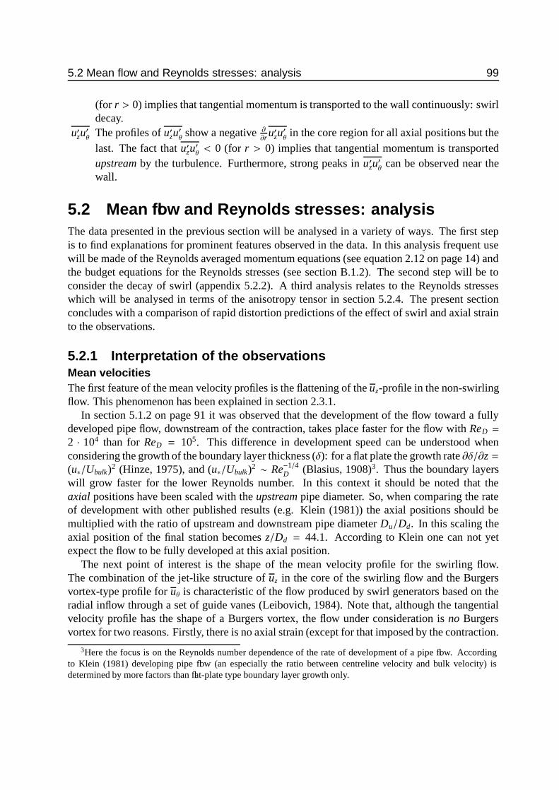
5.2 Mean flow and Reynolds stresses: analysis 99
(for r > 0) implies that tangential momentum is transported to the wall continuously: swirldecay.
u′zu′θ
The profiles of u′zu′θ
show a negative ∂∂r u′zu
′θ
in the core region for all axial positions but thelast. The fact that u′zu
′θ< 0 (for r > 0) implies that tangential momentum is transported
upstream by the turbulence. Furthermore, strong peaks in u′zu′θ
can be observed near thewall.
5.2 Mean flow and Reynolds stresses: analysisThe data presented in the previous section will be analysed in a variety of ways. The first stepis to find explanations for prominent features observed in the data. In this analysis frequent usewill be made of the Reynolds averaged momentum equations (see equation 2.12 on page 14) andthe budget equations for the Reynolds stresses (see section B.1.2). The second step will be toconsider the decay of swirl (appendix 5.2.2). A third analysis relates to the Reynolds stresseswhich will be analysed in terms of the anisotropy tensor in section 5.2.4. The present sectionconcludes with a comparison of rapid distortion predictions of the effect of swirl and axial strainto the observations.
5.2.1 Interpretation of the observationsMean velocitiesThe first feature of the mean velocity profiles is the flattening of the uz-profile in the non-swirlingflow. This phenomenon has been explained in section 2.3.1.
In section 5.1.2 on page 91 it was observed that the development of the flow toward a fullydeveloped pipe flow, downstream of the contraction, takes place faster for the flow with ReD =
2 · 104 than for ReD = 105. This difference in development speed can be understood whenconsidering the growth of the boundary layer thickness (δ): for a flat plate the growth rate ∂δ/∂z =(u∗/Ubulk)2 (Hinze, 1975), and (u∗/Ubulk)2 ∼ Re−1/4
D (Blasius, 1908)3. Thus the boundary layerswill grow faster for the lower Reynolds number. In this context it should be noted that theaxial positions have been scaled with the upstream pipe diameter. So, when comparing the rateof development with other published results (e.g. Klein (1981)) the axial positions should bemultiplied with the ratio of upstream and downstream pipe diameter Du/Dd. In this scaling theaxial position of the final station becomes z/Dd = 44.1. According to Klein one can not yetexpect the flow to be fully developed at this axial position.
The next point of interest is the shape of the mean velocity profile for the swirling flow.The combination of the jet-like structure of uz in the core of the swirling flow and the Burgersvortex-type profile for uθ is characteristic of the flow produced by swirl generators based on theradial inflow through a set of guide vanes (Leibovich, 1984). Note that, although the tangentialvelocity profile has the shape of a Burgers vortex, the flow under consideration is no Burgersvortex for two reasons. Firstly, there is no axial strain (except for that imposed by the contraction.
3Here the focus is on the Reynolds number dependence of the rate of development of a pipe flow. Accordingto Klein (1981) developing pipe flow (an especially the ratio between centreline velocity and bulk velocity) isdetermined by more factors than flat-plate type boundary layer growth only.

100 Analysis of laboratory measurements
Secondly, the width of the vortex core is mainly determined by the swirl generator, rather than byviscous diffusion of of what was originally a line vortex. The explanation of Leibovich is that theflow passing the vanes is essentially irrotational, giving an annulus of irrotational flow betweenthe core and the wall. The vortex core with positive vorticity, on the other hand, results fromthe boundary layer on the central body of the swirl generator. Leibovich explains the jet-likestructure of uz from a low centreline pressure due to shedding of the boundary layer from thecentral body. The low centreline pressure would result in an extra radial inflow4.
Another explanation of the jet near the centre line is that in the present set-up a part of theflow passes through the central body, resulting in an axial jet of its own right.
The increase of the centreline value of uz upon passage through the contraction is –qualitatively–in accordance with the inviscid analysis of Batchelor (1967) (see section 2.4.1) in which a flowwith uz(r) = U and uθ(r) = Ωr is passed through a contraction and the velocity profiles upstreamand downstream are compared assuming the flow to be cylindrical (∂/∂z = 0 and ur = 0) atboth axial positions. Unfortunately it is not possible to make a quantitative comparison betweenthe analysis of Batchelor and the present data, since the shape of the measured profiles is muchmore complicated than the simple flow considered by Batchelor. The same inviscid analysis pre-dicts an increase of uθ proportional to Dd/Du (i.e. conservation of angular momentum). Fromfigure 5.11 it can be seen that the integrated angular momentum is not conserved, but decreasessmoothly in the downstream direction. This is due to swirl decay. In order to remove the effectof swirl decay, the uθ-profiles have been replotted with uθ normalised with the ratio of actualangular momentum and a reference value of angular moment, i.e. at z/D = −5.8. The resultis shown in figure 5.12. The change in the shape of the uθ-profile as predicted by the inviscidanalysis is hardly visible in the data. In the ReD = 2 · 104 data there is a very slight steepeningdue to the axial strain. The data at the higher Reynolds number also show a steepening but thatoccurs already between x/D = −5.8 and −1.8. Figure 5.12 clearly shows the way in which theprofile of uθ changes downstream. Up to x/D = 6.9 there is a distinct vortex core extendingto roughly r/R = 0.5. Further downstream the profiles tend to a solid body rotation. Anotherstriking feature of the profiles is that –apart from the overall decrease in angular moment- thevortex core loses angular momentum and the wall region gains. The neutral point is located atr/R = 0.7 consistently for all profiles.
Reynolds normal stressesFor the non-swirling flow the most prominent phenomenon is the decrease of the normal stressesdue the axial strain. As remarked in section 5.1.2 this decrease is partly due to the scaling(with Ubulk
2). The unscaled profiles would show an increase of u′ru′r and u′θu′θ
and a decrease inu′zu′z. The explanation for this increase in u′ru′r and u′
θu′θ
is as follows: the axial strain stretchesvortices which have their axis in the z-direction and conservation of angular momentum requiresthat the vorticity ωz increases. Vortices with their axis in the radial and tangential direction are
4This explanation breaks down in flows where swirl decay plays a role: due to the decrease (in axial direction) ofuθ, the radial pressure gradient decreases which results in − ∂
∂z p being smaller in the centre than near the wall. Thisin turn gives a minimum in uz in the centre and possibly reverse flow (see e.g. Parchen and Steenbergen (1998);Kitoh (1991)).
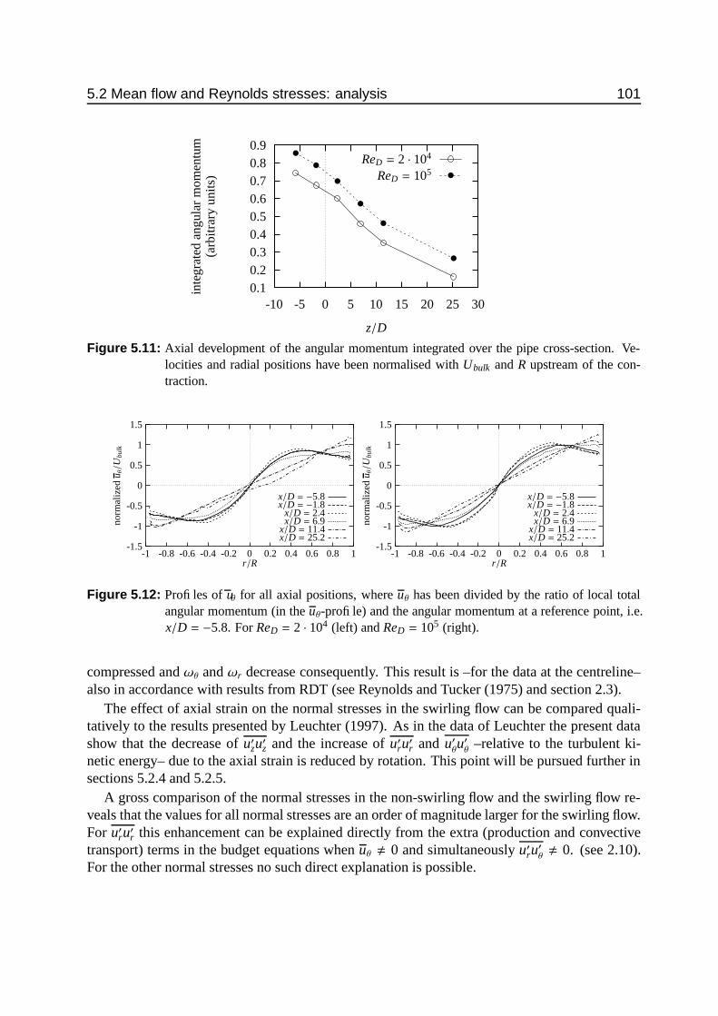
5.2 Mean flow and Reynolds stresses: analysis 101
ReD = 105ReD = 2 · 104
z/D
inte
grat
edan
gula
rm
omen
tum
(arb
itrar
yun
its)
302520151050-5-10
0.90.80.70.60.50.40.30.20.1
Figure 5.11: Axial development of the angular momentum integrated over the pipe cross-section. Ve-locities and radial positions have been normalised with Ubulk and R upstream of the con-traction.
x/D = 25.2x/D = 11.4
x/D = 6.9x/D = 2.4
x/D = −1.8x/D = −5.8
r/R
norm
aliz
edu θ/U
bulk
10.80.60.40.20-0.2-0.4-0.6-0.8-1
1.5
1
0.5
0
-0.5
-1
-1.5x/D = 25.2x/D = 11.4
x/D = 6.9x/D = 2.4
x/D = −1.8x/D = −5.8
r/R
norm
aliz
edu θ/U
bulk
10.80.60.40.20-0.2-0.4-0.6-0.8-1
1.5
1
0.5
0
-0.5
-1
-1.5
Figure 5.12: Profiles of uθ for all axial positions, where uθ has been divided by the ratio of local totalangular momentum (in the uθ-profile) and the angular momentum at a reference point, i.e.x/D = −5.8. For ReD = 2 · 104 (left) and ReD = 105 (right).
compressed and ωθ and ωr decrease consequently. This result is –for the data at the centreline–also in accordance with results from RDT (see Reynolds and Tucker (1975) and section 2.3).
The effect of axial strain on the normal stresses in the swirling flow can be compared quali-tatively to the results presented by Leuchter (1997). As in the data of Leuchter the present datashow that the decrease of u′zu′z and the increase of u′ru′r and u′
θu′θ
–relative to the turbulent ki-netic energy– due to the axial strain is reduced by rotation. This point will be pursued further insections 5.2.4 and 5.2.5.
A gross comparison of the normal stresses in the non-swirling flow and the swirling flow re-veals that the values for all normal stresses are an order of magnitude larger for the swirling flow.For u′ru′r this enhancement can be explained directly from the extra (production and convectivetransport) terms in the budget equations when uθ , 0 and simultaneously u′ru
′θ, 0. (see 2.10).
For the other normal stresses no such direct explanation is possible.

102 Analysis of laboratory measurements
Considering the shape of the profiles, one striking feature is the bump in the profiles near thecentreline for all stations between z/D = −5.8 and 6.9, inclusive. As far as the u′
θu′θ-stress is
concerned this maximum could be the result of vortex core precession (e.g. Escudier, 1987): asmall time-dependent radial displacement of the vortex core (with a large value of ∂
∂r uθ) gives alarge fluctuation in uθ. This interpretation suggests that the fluctuations in uθ do not representturbulent fluctuations but are –partly– the result of the meandering of the mean velocity field.Note that a bump in u′ru′r is a necessary consequence of the –assumed– axisymmetry of the flowin combination with a bump in u′
θu′θ. To make a quantitative estimate of the vortex displacement,
needed to explain the extra u′θu′θ-stress, the profiles at z/D = −5.8 with ReD = 2 · 104 will be
used as an example. The value of u′θu′θ
is about 0.025 above an estimated base value of 0.005(the value at r/R = 0.6). Thus the extra standard deviation in uθ, σ(uθ), is 0.16. The slope of theuθ-profile, ∂
∂r uθ, is about 1/0.3 ≈ 3.3. Consequently, a representative value for the vortex coredisplacement is σ(uθ)/ ∂
∂r uθ ≈ 0.05. This displacement –about 10% of the core diameter– is notimprobably large.
However, invocation of the possibility of vortex core precession can not explain the peak inu′zu′z near the centreline directly, since ∂
∂r uz = 0 at the centreline. An explanation that links thepeak in u′zu′z to that in u′
θu′θ
is that the uz-fluctuations may be produced through the pressure-straincorrelations (see 2.10): energy present in the ur and uθ fluctuations is transferred to the axialvelocity component.
Another explanation for the elevated levels of the normal stresses near the centreline is basedon the observation that the outflow of the swirl generator can be interpreted as two coaxially co-flowing jets. The inner jet has a relatively high axial velocity and has no tangential velocity. Theouter jet as a lower axial velocity and irrotational tangential velocity profile. This arrangementresults in a cylindrical shear layer in which both ∂
∂r uz and ∂∂r uθ are non-zero and fluctuations of
uz and uθ will be produced. This shear layer will grow radially and a certain axial position thecylindrical shear layer will disappear. The fluctuations of uz and uθ produced in the shear layerwill be carried downstream.
A third explanation is that fluctuations are produced at the swirl generator. According to theexplanation of Leibovich (1984), the vortex core must be interpreted as the remains of the bound-ary layer of the central body of the swirl generator. In that boundary layer, as well as in the zonewhere it is shed from the central body, the normal stresses will be enhanced. Furthermore, inthe current configuration of the swirl generator a part of the fluid passes through a round con-verging channel through the central body. In this channel extra uz-fluctuations will be produced.However, it is rather improbable that such elevated levels of fluctuations persist at a downstreamdistance of z/D ≈ 12 (the axial distance between swirl generator and first second measurementstation).
The three possible explanations for the elevated levels of fluctuations of uz and uθ differ in theaxial location of the production of the fluctuation: ranging from local production to productionin the swirl generator.

5.2 Mean flow and Reynolds stresses: analysis 103
Reynolds shear stress: u′ru′zFor the non-swirling flow the development of u′ru′z is rather straightforward. Upstream of thecontraction the profile of u′ru′z is –nearly– straight as is representative of a developed pipe flow.Downstream u′ru′z quickly attains its fully developed value in the near-wall region: somewherebetween z/D = 6.9 and 11.4. This distance appears to be in good agreement with the conclusionof Klein (1981) that the wall shear stress reaches the fully developed value after 8 to 15 diameters(4.6 < z/D < 8.6). Further downstream |u′ru′z| increases for the central part of the pipe as well.
The profiles of u′ru′z for the swirling flow need some closer examination. At z/D = −5.8 theaxial shear stress u′ru′z shows near-zero values for −0.5 < r/R < 0.5, which coincides with thevortex core (for ReD = 2 ·104 this region is somewhat smaller, as is the extent of the vortex core).These low values of |u′ru′z| may be an indication of the stabilising effect of rotation (see 2.2.2).Downstream of the contraction the profile of u′ru′z becomes nearly straight much quicker than inthe non-swirl case. One reason for this may be that the production term for u′ru′z (−u′ru′r
∂∂r uz) is
nearly shut off in the non-swirl case (due to the flat profile of uz), whereas in the swirling flowboth u′ru′r and − ∂
∂r uz are enhanced (the latter due to the bump in the uz-profile).
Reynolds shear stress: u′ru′θ
Upstream of the contraction the profile of u′ru′θ
shows a zero radial gradient in some parts ofthe vortex core (for z/D = −5.8 at ReD = 105 this region is largest), thus no tangential meanmomentum is transported outward in the core. In the rest of the pipe ∂
∂r u′ru′θ> 0 (for r > 0),
indicating decay of the swirl. Directly downstream of the contraction ∂∂r u′ru
′θ
is negative (forr > 0): the vortex core is fed from the outside. Negative values of u′ru
′θ
may be explained fromthe fact that production and convective transport terms in the budget of u′ru
′θ
become negativewhen u′ru′r > u′
θu′θ. This does not, however, explain the negative value for ∂
∂r u′ru′θ.
Reynolds shear stress: u′zu′θ
The profiles of u′zu′θ
are not easily interpreted. Whereas u′ru′z and u′ru′θ
stresses have a viscouscounterpart, the viscous shear stress σθz will be zero (since ∂
∂zuθ and ∂∂θ
uz are both –nearly– zero).
Upstream of the contraction, u′zu′θ< 0 for positive r. This is in accordance with the fact that
in the budget equation for u′zu′θ
both the production and convective transport terms are negative.Then, given the fact that u′zu
′θ= 0 at some point where the swirl has decayed, ∂
∂zu′zu′θ> 0 and thus
the axial gradient of u′zu′θ
is a loss term in the equation for uθ: u′zu′θ
appears to have a function inthe decay of swirl. Near the wall u′zu
′θ
is positive, which may be explained from the fact that inthe wall region long streaks of high and low streamwise velocity exist. In a non-swirling flowthis streamwise velocity is simply uz, but in a swirling flow this is a combination of uz and uθ.When such a streak passes, highly correlated fluctuations of uz and uθ will occur.
5.2.2 Development of the swirl numberIn the previous sections it has been observed frequently that for the swirling flow with axial straintwo processes produce axial variations of the flow: the axial strain exerted by the contraction and

104 Analysis of laboratory measurements
ReD = 105ReD = 2 · 104
z/D
S
302520151050-5-10
1
0.1
Figure 5.13: Axial development of the swirl number for ReD = 2 · 104 and 105. Note that the horizontalaxis shows the axial position scaled with the upstream pipe diameter, not the local diameter.Lines are drawn to connect points only. Error bars are drawn for the sake of completeness,but are hardly visible.
the decay of swirl due to wall friction. Numerous studies have been devoted to swirl decayin straight pipes (see section 2.2) and the aim of the present section is to see how the presentexperiment compares to previous results. In order to quantify the decay of swirl, some bulkmeasure of the ’amount of swirl’ is used in those studies. In most cases this is the swirl numberS , defined in equation 2.17, which will be employed here as well.
The main question is whether the axial strain has such influence on the flow that the swirldecay process downstream of the contraction is different from that found in straight pipes.
But first another question needs to be answered: what is the direct effect of the contraction onthe swirl ? This effect is twofold: on one hand the conservation of angular momentum results inan increase of the mean tangential velocity proportional to D−1, whereas on the other hand thebulk velocity increases proportionally to D−2. The net result on S is a decrease proportional to
a for axial region relative to contraction β for axial region relative to contraction
ReD upstream downstream upstream downstream
2 · 104 0.418 ± 0.0027 0.245 ± 0.0028 0.0245 ± 0.0017 0.0307 ± 0.0008105 0.483 ± 0.0022 0.274 ± 0.0039 0.0276 ± 0.0012 0.0214 ± 0.0008
Table 5.1: Fitting parameters in exponential decay of swirl (see equation 2.17) for the regions upstreamand downstream of the contraction. For the downstream region a 68% confidence interval isgiven. The error in the upstream decay coefficient is estimated assuming maximum errorswith opposite sign in the swirl numbers at z/D = −5.8 and −1.8. In the exponential decayformula the local pipe diameter has been used to normalise the axial position x.
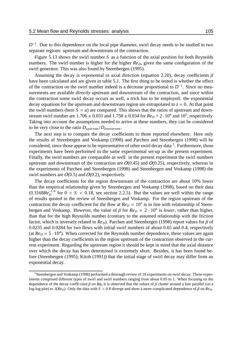
5.2 Mean flow and Reynolds stresses: analysis 105
D−1. Due to this dependence on the local pipe diameter, swirl decay needs to be studied in twoseparate regions: upstream and downstream of the contraction.
Figure 5.13 shows the swirl number S as a function of the axial position for both Reynoldsnumbers. The swirl number is higher for the higher ReD, given the same configuration of theswirl generator. This was also found by Steenbergen (1995).
Assuming the decay is exponential in axial direction (equation 2.20), decay coefficients βhave been calculated and are given in table 5.1. The first thing to be tested is whether the effectof the contraction on the swirl number indeed is a decrease proportional to D−1. Since no mea-surements are available directly upstream and downstream of the contraction, and since withinthe contraction some swirl decay occurs as well, a trick has to be employed: the exponentialdecay equations for the upstream and downstream region are extrapolated to z = 0. At that pointthe swirl numbers (here S = a) are compared. This shows that the ratios of upstream and down-stream swirl number are 1.706 ± 0.031 and 1.758 ± 0.034 for ReD = 2 · 104 and 105, respectively.Taking into account the assumptions needed to arrive at these numbers, they can be consideredto be very close to the ratio Dupstream/Ddownstream.
The next step is to compare the decay coefficients to those reported elsewhere. Here onlythe results of Steenbergen and Voskamp (1998) and Parchen and Steenbergen (1998) will beconsidered, since those appear to be representative of other swirl decay data 5. Furthermore, thoseexperiments have been performed in the same experimental set-up as the present experiment.Finally, the swirl numbers are comparable as well: in the present experiment the swirl numbersupstream and downstream of the contraction are O(0.45) and O(0.25), respectively, whereas inthe experiments of Parchen and Steenbergen (1998) and Steenbergen and Voskamp (1998) theswirl numbers are O(0.5) and O(0.2), respectively.
The decay coefficients for the region downstream of the contraction are about 10% lowerthan the empirical relationship given by Steenbergen and Voskamp (1998), based on their data(0.3168Re−1/4
D for 0 < S < 0.18, see section 2.2.5). But the values are well within the rangeof results quoted in the review of Steenbergen and Voskamp. For the region upstream of thecontraction the decay coefficient for the flow at ReD = 105 is in line with relationship of Steen-bergen and Voskamp. However, the value of β for ReD = 2 · 104 is lower, rather than higher,than that for the high Reynolds number (contrary to the assumed relationship with the frictionfactor, which is inversely related to ReD). Parchen and Steenbergen (1998) report values for β of0.0235 and 0.0284 for two flows with initial swirl numbers of about 0.65 and 0.4, respectively(at ReD = 5 · 104). When corrected for the Reynolds number dependence, these values are againhigher than the decay coefficients in the region upstream of the contraction observed in the cur-rent experiment. Regarding the upstream region it should be kept in mind that the axial distanceover which the decay has been determined is extremely short. Besides, it has been found be-fore (Steenbergen (1995); Kitoh (1991)) that the initial stage of swirl decay may differ from anexponential decay.
5Steenbergen and Voskamp (1998) performed a thorough review of 18 experiments on swirl decay. These exper-iments comprised different types of swirl and swirl numbers ranging from about 0.05 to 1. When focusing on thedependence of the decay coefficient β on ReD it is observed that the values of β cluster around a line parallel (on alog-log plot) to λ(ReD). Only the data with S > 0.8 diverge and show a more complicated dependence of β on ReD.

106 Analysis of laboratory measurements
5.2.3 Three-dimensionality in swirling flowTo study the possibly three-dimensional nature of the flow under consideration, the three anglesγ, γg and γτ have been computed (see section 2.2.4 for their definition).
In order to reduce the scatter –particularly– in γg, the velocity and stress data of positiveand negative r have been combined by averaging (this is warranted by axisymmetry observed insection 5.1.3). The result can be found in figure 5.14.
A number of observations can be made from this figure:
• The mean velocity profile is hardly skewed for r/R > 0.6 for most axial positions. Only thedata at z/D = 25.2 show a slight increase of γ with r (i.e. decrease with 1 − r/R).
• In the region r/R > 0.9 all three angles are of the same order, but differences of 100 to 200
do occur, mainly between γ and γτ on one hand, and γg on the other. However, the error γg
can easily be 100.• The stress roughly follows (within 200) the shear for a larger part of the pipe cross section
(r/R > 0.5, i.e. the region outside the vortex core) for most axial positions. Only at the sta-tion directly downstream of the contraction the relationship between shear and stress seemsto be disrupted: due to the axial strain both the u′ru′z and u′ru
′θ
profiles change significantly,whereas the mean velocity profiles hardly change.
• Inside the vortex core the shears are rather small (a flat uz-profile and near-solid body rota-tion for uθ). Still the shear angle γg seems to be well-defined, but the shear and the stressare not well aligned, which indicates the shear stresses are determined more by the flowupstream than by local processes.
It can be concluded that in this flow does not exhibit strong three-dimensionality in the senseof a skewed (or twisted) mean velocity profile in the wall-bounded part of the cross-section(r/R > 0.5). The shear and stress, however, are not aligned exactly, which indicates historyeffects or the absence of local equilibrium.
5.2.4 Comparison of stress-anisotropy between non-swirling andswirling flow
One of the problems in the comparison of the Reynolds stress data of the flows without and withswirl is the order of magnitude difference in their values. It is therefore more practical to presentthe data in terms of the normalised anisotropy tensor, aaa/k:
aaa = uuu′uuu′ − 23δδδk, (5.1)
where k is the turbulent kinetic energy. In the subsequent analysis the tensor aaa will be representedin cylindrical coordinates. The shear components of aaa will not be dealt with.
In figures 5.15 and 5.16 the normalised stress anisotropies are shown for ReD = 2 · 104 andReD = 105, respectively. When starting at the stations upstream of the contraction, it is manifestthat the flows with and without swirl are different. Whereas azz > 0 for the non-swirl flow, theswirling flow shows a nearly isotropic stress tensor in the centre, and azz < 0 in a large part of

5.2 Mean flow and Reynolds stresses: analysis 107
z/D806040200-20-40-60-80
80604020
0-20-40-60-80
806040200-20-40-60-80
80604020
0-20-40-60-80
806040200-20-40-60-80
βτ
βg
β
1 − r/R
angl
e(o )
10.1
80604020
0-20-40-60-80
25.2
11.4
6.9
2.4
contraction
−1.8
−5.8
806040200-20-40-60-80
806040200
-20-40-60-80
806040200-20-40-60-80
806040200
-20-40-60-80
806040200-20-40-60-80
βτ
βg
β
1 − r/R
angl
e(o )
10.1
806040200
-20-40-60-80
Figure 5.14: Indications of three-dimensionality in swirling flow: directions (in degrees) of mean flow(γ), shear (γg) and stress (γτ): ReD = 2 · 104 (left) and ReD = 105 (right). Assumingaxisymmetry the data for positive and negative r have been combined by averaging. Notethat the horizontal axis gives the distance to the wall 1 − r/R.

108 Analysis of laboratory measurements
z/Daθθ/karr/kazz/k
1
0.5
0
-0.5
-1
1
0.5
0
-0.5
-1
1
0.5
0
-0.5
-1
1
0.5
0
-0.5
-1
1
0.5
0
-0.5
-1
r/R
a zz/
k,a r
r/k,
a θθ/k
10.50-0.5-1
1
0.5
0
-0.5
-1
25.2
11.4
6.9
2.4
contraction
−1.8
−5.8
aθθ/karr/kazz/k
1
0.5
0
-0.5
-1
1
0.5
0
-0.5
-1
1
0.5
0
-0.5
-1
1
0.5
0
-0.5
-1
1
0.5
0
-0.5
-1
r/R
a zz/
k,a r
r/k,
a θθ/k
10.50-0.5-1
1
0.5
0
-0.5
-1
Figure 5.15: Normalised anisotropies of normal stresses at ReD = 2 · 104 for flow without swirl (left)and with swirl (right)
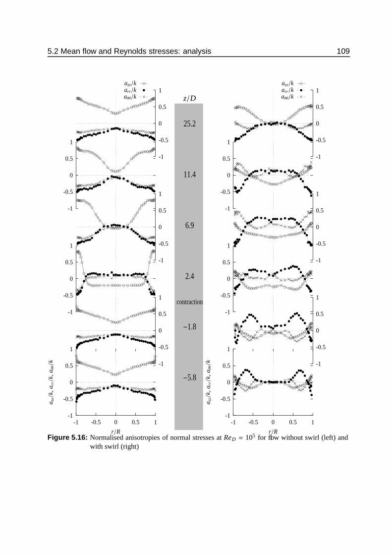
5.2 Mean flow and Reynolds stresses: analysis 109
z/Daθθ/karr/kazz/k
1
0.5
0
-0.5
-1
1
0.5
0
-0.5
-1
1
0.5
0
-0.5
-1
1
0.5
0
-0.5
-1
1
0.5
0
-0.5
-1
r/R
a zz/
k,a r
r/k,
a θθ/k
10.50-0.5-1
1
0.5
0
-0.5
-1
25.2
11.4
6.9
2.4
contraction
−1.8
−5.8
aθθ/karr/kazz/k
1
0.5
0
-0.5
-1
1
0.5
0
-0.5
-1
1
0.5
0
-0.5
-1
1
0.5
0
-0.5
-1
1
0.5
0
-0.5
-1
r/R
a zz/
k,a r
r/k,
a θθ/k
10.50-0.5-1
1
0.5
0
-0.5
-1
Figure 5.16: Normalised anisotropies of normal stresses at ReD = 105 for flow without swirl (left) andwith swirl (right)
110 Analysis of laboratory measurements
the pipe cross-section. In the swirling flow the radial component of aaa dominates and azz andaθθ behave much alike. Directly downstream of the contraction (z/D = 2.4) this picture haschanged dramatically. The flows with and without swirl have very similar profiles of the normalcomponents of aaa (especially for ReD = 2 · 104): azz has become negative and arr and aθθ areslightly positive for |r/R| < 0.8 (arr , aθθ at the centreline for some stations, which is incorrectif axisymmetry is assumed). In the region 0.8 < |r/R| < 1 aθθ follows arr for the non-swirl case.Furthermore, the profile of arr for the swirling flow is similar to that of the non-swirling flow.On the other hand, aθθ in the swirling flow shows a deviant behaviour. This results from the factthat the mean streamwise direction in the swirling flow has a θ-component as well, whereas inthe non-swirling flow the mean flow is in the z-direction. Thus one should compare the sum ofaθθ and azz. This comparison shows that indeed the swirl case and the non-swirl case behavesimilarly (not shown). Another indication that this explanation is correct is the observation (seesection 5.2.3) that in the wall region the flow is hardly three-dimensional: mean flow and stressesare aligned.
The change in anisotropy due to the axial strain is less for the swirl flow than for the non-swirling flow, since the initial anisotropies are smaller for the first case. Leuchter (1997) showsthat this can be attributed to a rotation-induced enhancement of the linear (so-called ’rapid’)pressure strain term.
Focusing on the downstream development of aaa, downstream of the contraction, it is clear thatthe relaxation from the effects of the axial strain is much quicker for the non-swirling flow thanfor the swirling flow. At the centreline of the swirling flow azz attains a zero value (which isthe value upstream of the contraction) only at z/D = 25.2 for ReD = 2 · 104 and somewherebetween z/D = 11.4 and 25.2 for ReD = 105. In the non-swirling flow, however, azz changessign at the centreline near z/D = 6.9. The slow relaxation of the swirling flow suggests thatthe pressure-strain correlations (see (2.10)), which are the main mechanism to exchange energybetween normal stresses, are suppressed by the rotation. Given the fact that Leuchter (1997)shows that the linear part of the pressure strain terms is enhanced by rotation, it is probably thenonlinear part that is reduced (and the linear part is of minor importance when the large-scalestrain is no longer applied).
In order to focus on the downstream development of the stress-anisotropy, figures 5.17 and5.18 show the axial development of aaa at the centreline for ReD = 2 · 104 and 105, respectively. Itappears that the change in aaa due to the axial strain is less dramatic for the swirling flow than itis for the non-swirling flow. This is in accordance with the findings of Leuchter (1997). Anothernotable feature is that for the flow without swirl there is only a minor difference between the twoReynolds numbers. However, the swirling flow at ReD = 2 · 104 at axial position z/D = 25.2shows values of aaa much alike the non-swirling flow, whereas the flow at ReD = 105 at the sameposition has only arrived at the pre-contraction values of aaa. One should keep in mind that thedownstream development of the swirling flow is complicated by the simultaneous swirl decay(see the previous section): the swirl number decreases between z/D = 2.4 and 25.2 by 71% and57% for ReD = 2 · 104 and 105, respectively.
Another way to view the anisotropy of the Reynolds stresses is by using the stress tensor

5.2 Mean flow and Reynolds stresses: analysis 111
z/D
a zz/
k,a r
r/k,
a θθ/k
302520151050-5-10
0.30.20.1
0-0.1-0.2-0.3
aθθ/karr/kazz/k
z/D
a zz/
k,a r
r/k,
a θθ/k
302520151050-5-10
0.30.20.1
0-0.1-0.2-0.3
Figure 5.17: Axial development of the stress anisotropies at the centreline at ReD = 2 · 104: non-swirlcase (left) and swirling flow (right). Note that the lines only serve to connect the observa-tions.
z/D
a zz/
k,a r
r/k,
a θθ/k
302520151050-5-10
0.30.20.1
0-0.1-0.2-0.3
aθθ/karr/kazz/k
z/D
a zz/
k,a r
r/k,
a θθ/k
302520151050-5-10
0.30.20.1
0-0.1-0.2-0.3
Figure 5.18: Axial development of the stress anisotropies at the centreline at ReD = 105: non-swirl case(left) and swirling flow (right).
invariants. Usually the invariants of the anisotropy tensor (see equation 5.1) are used:
II = −12
ai ja ji (5.2)
III =13
ai ja jkaki (5.3)
van Dijk (1999) points out that the disadvantage of II is that it depends quadratically on a linearchange –due to distortion– in the eigenvalues of the stress tensor. He proposes the followingmodified invariants:
II∗ = 63
√III2
(5.4)
III∗ = 3√−II (5.5)
Due to conditions of realisability not all combinations of II∗ and III∗ are physically possible.A sketch of the domain of II∗ and III∗ is given in figure 5.19 along with interpretations of the

112 Analysis of laboratory measurements
limits. The only possible combinations of II∗ and III∗ are within the triangular shape. In theorigin the stress tensor is fully isotropic. Both straight lines starting at the origin are the limitsof axisymmetric turbulence. To the left of III∗ = 0 the stress tensor has two major axes and oneminor axis (pancake), whereas to the right there is one major axis and two minor axes (cigar).The upper limit of the area of realisable stress tensors is the limit of 2-component turbulence(sometimes called two-dimensional. The idea of plotting II and III in such a diagram comesfrom Lumley (1978), the modified Lumley triangle is due to van Dijk (1999).
Figure 5.20 the modified Lumley-diagram is shown with data from the non-swirling flow andthe swirling flow, both for ReD = 105. Each symbol in the plot represents one radial position. Thedata are split into a core region |r|/R < 0.7 and a wall region |r|/R > 0.7. The limits are basedon the observed indifference to swirl decay of the uθ-profile normalised with the total angularmomentum (see figure 5.12).
In the non-swirling flow the turbulence is nearly axisymmetric for all axial positions: thestress tensor has one major axis (i.e. cigar-type anisotropy). The stress tensor is more isotropicnear the pipe axis than near the wall. Only directly downstream of the contraction, the turbulencebecomes non-axisymmetric for some radial positions. Furthermore, in the region |r|/R < 0.7 theanisotropy is of pancake type (i.e. two major axes). At z/D = 6.9 the flow already has recoveredfrom this disturbance, although the stress tensor is more isotropic near the centre here than in theflow upstream of the contraction.
For the swirling flow the situation is less clear. For all axial positions there are (radial) pointswhere the turbulence is not axisymmetric. The effect of the contraction is to move more pointsin the direction of pancake type axisymmetry, although only the near-wall points show someaxisymmetry of the turbulence. Further downstream, at z/D = 11.4 the turbulence is nearlyaxisymmetric in a large part of the pipe cross section, being of the pancake type. Betweenz/D = 11.4 and z/D = 25.2, however, all points move from the left side to the right side: frompancake to cigar type of axisymmetry. This is due to the fact that due to swirl decay the roleof u′
θu′θ
and associated shear stresses has diminished when compared to upstream positions. Theflow becomes more like a developed pipe flow.
When comparing the graphs of non-swirling and swirling flow it is apparent that near thepipe axis the contraction has opposite effects. For the non-swirling flow the contraction leadsto a more isotropic stress tensor, whereas in the swirling flow the contraction makes it moreanisotropic. In both cases the effect of the contraction disappears further downstream.
5.2.5 Rapid distortion analysis of normal stresses at centrelineIn order to see to what extent the observed development of stress anisotropies can be explainedby linear effects, a simple rapid distortion calculation has been made. For the data withoutswirl, the analytical results of analysis of Batchelor and Proudman (1954) can be used, with theextensions of Reynolds and Tucker (1975) to take into account initial anisotropy. No analyticalresults are given for distortions that include rotation, however. Therefore, the rapid distortion hasbeen computed numerically with the following procedure:
• Only the pipe axis is considered. This implies that the distortion is axisymmetric.

5.2 Mean flow and Reynolds stresses: analysis 113
III*
II*
axisymmetric
pancake cigar
axisy
mmetric
isotropy
2 component turbulence
0
0.5
1
1.5
2
−1 −0.5 0 0.5 1 1.5 2
Figure 5.19: Modified Lumley-triangle (after van Dijk (1999)). The horizontal axis is a measure ofelongation of the stress tensor (with isotropy at III∗ = 0) and the vertical axis is a measureof anisotropy (with isotropy at II∗ = 0).
• An initial isotropic spectrum is computed using the model spectrum due to Von Karman(taken from Hultgren and Cheng (1983)).
• In order to obtain anisotropic initial normal stresses, an initially isotropic spectrum is subjectto an axial strain until the stresses exhibit the required anisotropy. This method was alsoused by Cambon and Jacquin (1989) and is similar to the trick used by Reynolds and Tucker(1975).
• The initial anisotropy is taken from the data of the station directly upstream of the contrac-tion (i.e. 1.8 diameters upstream).
• Since the strain is not constant inside the contraction, the strain is applied step-by-step.After each small time-step the strain is recalculated given the pipe diameter for that axialposition.
• For the axial strain without rotation, the strain is determined assuming a uniform axialvelocity that is proportional to D−2. For the flow with axial strain and rotation, the axialstrain is computed identically. The tangential velocity profile is determined assuming asolid-body rotation, of which the angular velocity is proportional to D−1. The initial angularvelocity is taken from the observed ∂
∂r uθ at the centre, upstream of the contraction.• The normal stresses of which the anisotropy is studied are obtained by integration of the
spectrum.• The RDT calculations have been started at the start of the contraction (z/D = 0) using
observed ansiotropies from (z/D = −1.8) and continued arbitrarily until the axial positionof the first observations downstream of the contraction (z/D = 2.4).

114 Analysis of laboratory measurements
z/D
|r|/R > 0.7|r|/R ≤ 0.7
III∗
II∗
21.510.50-0.5-1
2
1.5
1
0.5
0
25.2
11.4
6.9
2.4
contraction
−1.8
−5.8
|r|/R > 0.7|r|/R ≤ 0.7
III∗
II∗
21.510.50-0.5-1
2
1.5
1
0.5
0
Figure 5.20: Modified Lumley plots for flow without swirl (left) and with swirl (right). Re D = 105. Eachsymbol represents one radial position.

5.2 Mean flow and Reynolds stresses: analysis 115
arr/k RDTazz/k RDTarr/k dataazz/k data
x/D
a zz/
kor
a rr/
k
3210-1-2
0.3
0.2
0.1
0
-0.1
-0.2
-0.3
-0.4
-0.5arr/k RDTazz/k RDTarr/k dataazz/k data
x/D
a zz/
kor
a rr/
k
3210-1-2
0.3
0.2
0.1
0
-0.1
-0.2
-0.3
-0.4
-0.5
Figure 5.21: Comparison of stress anisotropies at the axis as predicted by RDT, as well as observedvalues. The observations are indicated by single symbols, whereas the RDT results areindicated with a line, labeled with symbols at start and end. Observations are for ReD =
105. The RDT calculations have been started at the start of the contraction (z/D = 0) andcontinued arbitrarily until the axial position of the first observations downstream of thecontraction (z/D = 2.4). The contraction is located at 0 < z/D < 0.6.
Figure 5.21 shows the results of the RDT analysis together with the observed stress anisotropiesfor ReD = 105. For the non-swirl case the observations at z/D = −1.8 and z/D = 2.4 can beassumed to be representative for those at the entrance and exit of the contraction, since in theregions upstream and downstream no strain acts on the turbulence. Then RDT appears to givea good prediction of the anisotropy for the non-swirl case. The RDT analysis clearly shows azz
and arr change sign due to the axial strain.
For the flow with swirl the situation is more complicated, since then also in the regions up-stream and downstream of the contraction a strain is present (due to the swirl). The effect of thisstrain can be seen clearly in the RDT results downstream of the contraction (z/D > 0.6) wherethe anisotropies continue to change, but in a direction opposite to that inside the contraction:there is a tendency to a return to a more isotropic situation. This linear effect of rotation on theanisotropy will certainly be present outside the contraction. However, over distances much largerthan the length of the contraction, nonlinear effects will mask this linear effect of rotation. Giventhe distance of about two pipe diameters between the upstream observations and the entrance,as well as between the exit of the contraction and the downstream observations, the RDT resultscan be compared to the observations only qualitatively. The effect of the addition of rotationto the axial strain is to slightly diminish the change in anisotropy inside the contraction, whencompared to the non-swirl case. This is in accordance with the data of (Leuchter and Dupeuble,1993). The present data, however, suggest a very strong reduction in the change in anisotropy.This may be attributed to the linear effect of rotation in the region outside the contraction (pos-sibly both upstream and downstream). When taking into account the observations downstreamof z/D = 2.4 however, it becomes clear that downstream of the contraction the linear effect ofrotation must be overwhelmed by nonlinear effects: up to z/D = 6.9 the anisotropies increase (inan absolute sense), rather than decrease as suggested by the RDT results.

116 Analysis of laboratory measurements
5.3 Analysis of time series dataIn this sections two quantities will be discussed that give information about the spatial structureof the turbulence: the one-dimensional spectra and the integral scales.
5.3.1 SpectraThe analysis of the experimental data concludes with a look at the spatial structure of the turbu-lent velocity field by means of one-dimensional spectra and integral length scales. These spectrahave been determined from the raw data gathered (see section 3.3). Only data for ReD = 105 willbe shown, since the data for ReD do not show a clear inertial subrange and appear to suffer fromambiguity noise (see 3.1.3) and aliasing (due to deficiencies in the low-pass filter in the trackers,see section 3.3.3).
Figure 5.22 shows the axial development of power spectra at the pipe axis: the one-dimensionaluz-spectrum and ur-spectrum. The flows without swirl and with swirl will be discussed sepa-rately. Although according to Tennekes and Lumley (1972) no inertial subrange is to be expectedat this modest Reynolds number, the data suggest that for most stations a region with a slope ofthe order of k−5/3 exists above kD = 5. For the non-swirling flow the effect of the contractionis mainly that uz fluctuations are suppressed at large scales (small k) and fluctuations in ur areenhanced at large scales, while being suppressed at small scales. These effects of the contractionhave disappeared again at z/D = 25.2. Furthermore, between z/D = −1.8 and z/D = 2.4, thevalues of Fzz at the origin decreases whereas the value of Frr increases. Since Fii/u′iu
′i is propor-
tional to the integral length scale L (Tennekes and Lumley, 1972), Lrr increases and Lzz decreases(see 2.3.2 on page 26).
For the data of the swirling flow the spectra upstream of the contraction exhibit a slope steeperthan −5/3, even suggesting the two-dimensional limit of k−3. Downstream of the contraction thedata suggest a −5/3 slope. Another feature of the downstream spectra is that the large-scale partof the spectrum has shifted to smaller wave numbers. A related phenomenon is that the valuesfor Fii at the origin are larger than those for the non-swirling flow. Thus L will be larger for theswirling flow compared to the non-swirling flow (see below). A final remark is that the exchangeof energy between u′zu′z (minus) and u′ru′r (plus) as observed in the non-swirling flow is not clearlypresent in the swirling flow.
Figure 5.23 shows the one-dimensional spectra at the radial location r/R = 0.9 for uz, ur anduθ. Again the non-swirling and swirling flow will be dealt with separately. The non-swirlingdata show a clearer inertial subrange than for the pipe-axis data in figure 5.22 but above a higherwavenumber (kD > 20 upstream of the contraction, kD > 5 downstream). The effect of the con-traction is similar for all three spectra: small scales are suppressed and large scales are enhanced.The effect is strongest for uθ. At the axial position z/D = 11.4 the spectra have recovered alreadyfrom the disturbance of the contraction.
The swirling flow spectra do not show a region with a spectral slope of −3, but rather have aninertial subrange with k−5/3. This suggests that at r/R = 0.9 is not so much influenced by rotationbut rather behaves as a normal shear flow. The effect of the contraction on enhancement of largescales, relative to small scales is similar as for the non-swirling case, and again the effect of theuθ spectrum is largest. The shift of the large-scale part of the spectrum to smaller wave numbers

5.3 Analysis of time series data 117
x/D =25.2x/D =11.4
x/D =6.9x/D =2.4
x/D =-1.8x/D =-5.8
k−5/3
kD (-)
Fzz/u′ zu′ z
(arb
itrar
yun
its)
1001010.10.01
10000
1000
100
10
1
0.1
0.01
0.001
0.0001
1e-05
1e-06
x/D =25.2x/D =11.4
x/D =6.9x/D =2.4
x/D =-1.8x/D =-5.8
k−3
k−5/3
kD (-)
Fzz/u′ zu′ z
(arb
itrar
yun
its)
1001010.10.01
10000
1000
100
10
1
0.1
0.01
0.001
0.0001
1e-05
1e-06
k−5/3
kD (-)
Frr/u′ ru′ r
(arb
itrar
yun
its)
1001010.10.01
10000
1000
100
10
1
0.1
0.01
0.001
0.0001
1e-05
1e-06
k−3
k−5/3
kD (-)
Frr/u′ ru′ r
(arb
itrar
yun
its)
1001010.10.01
10000
1000
100
10
1
0.1
0.01
0.001
0.0001
1e-05
1e-06
Figure 5.22: One-dimensional spectra at the pipe centreline: uz-spectrum (top) and ur spectrum (bot-tom), without swirl (left) and with swirl (right). Only data for ReD are shown. The spectrafor axial positions z/D > −5.8 are shifted upward by a factor of 10 for each axial position.The wavenumber has been determined from the frequency and the mean axial velocity.Normalisation of k has been done with the local pipe diameter. The spectra have beenaveraged over logarithmically spaced bins.

118 Analysis of laboratory measurements
x/D =25.2x/D =11.4
x/D =6.9x/D =2.4
x/D =-1.8x/D =-5.8
k−5/3
kD (-)
Fzz/u′ zu′ z
(arb
itrar
yun
its)
1001010.10.01
10000
1000
100
10
1
0.1
0.01
0.001
0.0001
1e-05
1e-06
x/D =25.2x/D =11.4
x/D =6.9x/D =2.4
x/D =-1.8x/D =-5.8
k−3
k−5/3
kD (-)
Fzz/u′ zu′ z
(arb
itrar
yun
its)
1001010.10.01
10000
1000
100
10
1
0.1
0.01
0.001
0.0001
1e-05
1e-06
k−5/3
kD (-)
Frr/u′ ru′ r
(arb
itrar
yun
its)
1001010.10.01
10000
1000
100
10
1
0.1
0.01
0.001
0.0001
1e-05
1e-06
k−3
k−5/3
kD (-)
Frr/u′ ru′ r
(arb
itrar
yun
its)
1001010.10.01
10000
1000
100
10
1
0.1
0.01
0.001
0.0001
1e-05
1e-06
k−5/3
kD (-)
Fθθ/u′ θu′ θ
(arb
itrar
yun
its)
1001010.10.01
10000
1000
100
10
1
0.1
0.01
0.001
0.0001
1e-05
1e-06
k−3
k−5/3
kD (-)
Fθθ/u′ θu′ θ
(arb
itrar
yun
its)
1001010.10.01
10000
1000
100
10
1
0.1
0.01
0.001
0.0001
1e-05
1e-06
Figure 5.23: One dimensional spectra r/R = 0.9: uz-spectrum (top) and ur-spectrum (middle) and uθ-spectrum (bottom), without swirl (left) and with swirl (right). The uz and ur spectra havebeen obtained with the LDA optics displaced vertically from the pipe axis, whereas theuθ have been measured with the LDA displaced horizontally (along its optical axis). Forfurther information see caption of figure 5.22.

5.3 Analysis of time series data 119
is similar to what happens in the swirling flow spectra at the pipe axis.A difficulty in the interpretation of the swirling flow spectra in figure 5.23 is that the spectra
of uz and uθ are a combination of longitudinal and transverse spectra: the longitudinal directionis along the mean flow direction, whereas the velocity components are parallel and perpendicularto the pipe axis. The angle between mean flow direction and axial direction ranges from 400 to200 at r/R = 0.9 (see figure 5.14). Therefore, the spectra have been recomputed with velocitycomponents rotated in the direction of the mean flow. The results, however, hardly differ fromthe spectra shown in figure 5.23 and are not shown therefore.
5.3.2 Integral scalesAnother measure of the spatial structure of the turbulent field is the integral length scale, L, of agiven velocity component (or scalar, if applicable).
Formally the integral length scale equals the integral of the autocorrelation function6. It is ameasure of the largest scales present in the turbulence. When using one-point measurements onecan only determine the integral length scale in the direction of the mean flow. In a non-swirlingflow the integral length scale for uz will be a longitudinal length scale, whereas the scale for ur
and uθ will be a transverse length scale. In case of swirl the situation is less clear. Then onlythe integral scale for ur will be a real transverse scale, whereas the integral scales for uz and uθwill be a mix of longitudinal and transverse. Here, the integral length scale will be estimatedfrom the integral time scale by converting the time lag into a spatial lag using the mean axial (notstreamwise) velocity.
Figure 5.24 shows the axial development of the integral length scales at the pipe axis. Theeffect of the contraction is to decrease Lzz and to enhance the two transverse length scales. Thisis in accordance with results from rapid distortion theory. The length scales recover surprisinglyquickly from the distortion due to the contraction. For the swirling flow the length scales up-stream of the contraction are nearly isotropic (as are the Reynolds stresses as observed earlier).The effect of the contraction on Lrr and Lθθ is much larger than in the non-swirling case. Thelength scales have grown up to 1.8 times the pipe diameter. Furthermore, Lzz increases ratherthan decreases.
In figure 5.25 the length scales are shown for a radial position r/R = 0.9. For the non-swirlingflow Lrr and Lθθ behave qualitatively the same as at r/R = 0. On the other hand, Lzz increases dueto the contraction whereas it decreases at the centreline. For the swirling flow however, Lθθ andLzz are similar in the near wall region. This can be understood from the fact that both uz and uθexhibit strong shear in the near-wall region. This also explains the fact that the axial developmentof both Lθθ and Lzz in the swirling flow is similar to the development of Lzz in the non-swirlingflow. The similarity between Lθθ and Lzz might also be due to the method of analysis: the lengthscale is in the direction of the mean flow, whereas the velocity components are not exactly inestreamwise and cross-stream direction. However, in the discussion of spectra in the previoussection it was observed that this is a small effect.
6By definition, however, the autocorrelation function in one-point measurements integrates to zero, resultingin zero integral length scale. Therefore the autocorrelation function is integrated between zero time-lag and thesmallest time-lag until where the autocorrelation function changes sign.

120 Analysis of laboratory measurements
Lθθ/DLrr/DLzz/D
z/D
Lii/D
302520151050-5-10
0.50.45
0.40.35
0.30.25
0.20.15
0.10.05
0
Lθθ/DLrr/DLzz/D
z/D
Lii/D
302520151050-5-10
2
1.5
1
0.5
0
Figure 5.24: Axial development of integral length scales of the normal stresses for ReD = 105: non-swirling flow (left) and swirling flow (right). The data refer to r/R = 0. The length scaleshave been scaled with the upstream pipe diameter. Note the difference in vertical scalebetween the two plots. The lines are drawn only to clarify the relationship between differentpoints.
Lθθ/DLrr/DLzz/D
z/D
Lii/D
302520151050-5-10
1.2
1
0.8
0.6
0.4
0.2
0
Lθθ/DLrr/DLzz/D
z/D
Lii/D
302520151050-5-10
1.2
1
0.8
0.6
0.4
0.2
0
Figure 5.25: Axial development of integral length scales of the normal stresses for ReD = 105: non-swirling flow (left) and swirling flow (right). The data refer to r/R = 0.9. The lines aredrawn only to clarify the relationship between different points.
5.4 To concludeIn the previous sections the experimental data have been analysed in a variety of ways and it iswell possible to get lost in the overwhelming amount of results. Here an attempt will be made toassemble a clear picture of the flow under consideration. The results for the flow without swirland with swirl will be discussed separately.
5.4.1 Axial strain without swirlThe mean axial velocity is transformed from a profile representative of fully developed pipe flowto a flat profile as in the entrance region of a pipe. Also the normal stresses are nearly uniformacross the pipe cross-section, and the shear stress u′ru′z is small except near the walls. The effect ofthe axial strain on the anisotropy of the normal stresses is to reverse the signs of the anisotropiesof u′zu′z on one hand and u′ru′r and u′
θu′θ
on the other. This effects is well described by linear theory

5.4 To conclude 121
(RDT).Approximately 40 pipe diameters downstream of the contraction (downstream pipe diameters)
the profiles of the mean velocity and the normal stress have returned to their fully developedshape. The shear stress u′ru′z has not yet completely relaxed at that axial position, however. Therelaxation toward the fully developed profiles occurs first near the wall. Further downstream, theregion of the pipe cross-section affected by this development grows toward the pipe axis.
5.4.2 Axial strain with swirlThe effect of the axial strain on the profiles of uz and uθ near the pipe axis is in accordance withthe inviscid analysis of Batchelor (1967): uz develops a bump and uθ becomes slightly curvedrather than straight. The swirl decay rate seems not to change dramatically by the axial strain.The swirling flow is not skewed for large part of the near-wall region, so there are no indicationsfor a three-dimensional boundary layer.
Upstream of the contraction the Reynolds stress tensor (at the pipe axis) in the swirling flowis more isotropic than that in the non-swirling flow. The effect of the axial strain on the stressanisotropy is weaker than for the non-swirling flow. This is –qualitatively– predicted by RDTtheory. Directly downstream the anisotropies of the stress tensor are very similar for the swirlingand non-swirling flow, but further downstream they diverge again. At the position, furthestdownstream from the contraction, there is a clear distinction between the two Reynolds num-bers: for the lower Reynolds number, the stress anisotropy is close to that for the non-swirlingflow, whereas for the high Reynolds number, there is a large difference between swirling andnon-swirling flow. This may have two reasons: the swirl decays faster for the lower Reynoldsnumber, and the travel time from the contraction is a factor of 5 longer for the lower Reynoldsnumber. The character of the stress tensor throughout the pipe cross section differs considerablybetween the non-swirling and swirling flow. In the non-swirling flow the turbulence is nearlyaxisymmetric at the vast majority of axial and radial positions: the stress tensor has one majoraxis. In the swirling flow, the turbulence is not axisymmetric at most locations. Near the wall,the tensor is pancake-shaped (two major axes), near the pipe axis there is one major axis.
The effect of axial strain on the structure of the turbulence is that in the swirling flow muchenergy is transferred to larger scales, especially for ur and uθ. This translates into large integrallength scales.
All results for the swirling flow suggest that a clear distinction can be made between a coreregion (roughly r/R < 0.7) and an outer region. In the core rotational effects play an importantrole. On the other hand, the near wall region behaves like a normal shear flow, despite the largeangle between mean flow and axial direction.

122 Analysis of laboratory measurements

6 Results of numericalsimulations
In this chapter the results of the simulations will first be compared with the measured data.Besides, additional analyses will be made, focusing on the terms in the budgets of Reynoldsstresses and on what happens within the contraction. Details on the setup of the simulations canbe found in section 4.3.
6.1 Validation of the LES resultsIn this section the LES results will be confronted with the results from the laboratory experi-ment, discussed in chapter 5. The results for the flow without and with swirl will be dealt withseparately. Two measurement stations of the experimental setup fall within the domain of thesimulation, viz. those at z/D = −1.8 and 2.4. The data at those two locations will be used for themodel validation.
6.1.1 A note on the presentation of resultsIn the intercomparison of laboratory data and simulation results a number of discrepancies needto be resolved:
• For the laboratory measurements, the radial coordinate is made dimensionless with the piperadius, whereas in the model the pipe diameter is used. In the present chapter all radialcoordinates will be normalised with the local pipe radius.
• The velocities in the laboratory measurements are originally normalised with the local bulkvelocity (see previous chapter), whereas in the model the friction velocity of the pipe sectionupstream of the contraction is used. In the presentation of the data, all velocities will benormalised with the local friction velocity. Since no friction velocity data are available forthe laboratory data, the ratio between bulk velocity and friction velocity from the simulationis used. This implies that an error in the ratio Ubulk/u∗ in the simulation, results in anincorrect representation of the LDA data. In fact, the normalisation used here is equivalentto a normalisation of both simulation results and LDA data with the bulk velocity (obtainedfrom the present presentation by multiplying velocities with the ratio u∗/Ubulk from thesimulation). At both axial positions the velocities and stresses are normalised with the localmodel friction velocity.
• In order to make laboratory data and measurements comparable, the simulation results ofReynolds stresses include both the resolved and the sub-grid scale stresses. To show thecontribution of the subgrid stress to the total stress, the subgrid contribution is also shownseparately. The sub-grid contribution to the normal stresses consists of the anisotropic part
123

124 Results of numerical simulations
of the stress (taken into account by the sub-grid scale stress model) and the isotropic part.The latter is non-existent in the model, since it has been lumped with the dynamic pressure(see equation 4.6). For the presentation of the normal stresses, the isotropic part has beendetermined from the sub-grid kinetic energy (ES GS ), using equation 4.14.
• Since the simulation data are averaged over a full circumference of the pipe, only data for0 < r/R < 1 are available. Therefore the measurement data are plotted against |r/R|, ratherthan r/R. As a consequence, two datapoints will appear for each radial position |r/R|, viz.one for r < 0 and one for r > 0.
• The experimental data are accompanied by estimates of the error (or tolerance) in the data(although in some cases the error bars are hardly visible). For the simulation data a similarerror analysis has been made. The resulting range is indicated by plotting two lines: onethat gives the upper bound of the simulated value and one that gives the lower bound (95%tolerances are used). In many cases the three lines can not be discerned. For details on theerror estimates see appendix A.
• The LES data for z/D = −1.8 are obtained from the model with periodic boundary condi-tions and constant radius, whereas the data downstream of the contraction (z/D = 2.4) aretaken from the model with varying pipe diameter, as described in section 4.2. The modeldomain extended from over −1.8D < z < 4.2D. Consequently, of all the experimental datapresented in chapter 5, only the data at z = −1.8D and z = 2.4D can be used for validation.
6.1.2 Flow with axial strainIn this section the results of the LES of the flow with axial strain but without swirl will bepresented. Table 6.1 summarises the key features of the simulation. Some noteworthy factsare:
• The bulk velocity attained upstream of the contraction (and consequently downstream) isvery close to the value of the laboratory experiment.
• The turbulent Reynolds number increases strongly downstream of the contraction due to thelarge increase in the wall friction (and thus u∗). Since the flow is an axially inhomogeneousflow, the value quoted is valid only for the given axial location (z/D = 2.4) in the modeldomain (and will probably decrease further downstream).
• Due to the increase in u∗, the resolution in terms of viscous wall units decreases (i.e. be-comes coarser). Thus, despite the fact that downstream of the contraction the gridcells aresmaller, effectively the resolution decreases.
The results for the mean flow, as well as the turbulent stresses are shown in figures 6.1 to6.6. The simulated profiles of the mean axial velocity match the measurements very closely(i.e. are indistinguishable) upstream of the contraction (figures 6.1 and 6.2). Downstream ofthe contraction the match is close, but the tolerance intervals do not overlap. Upstream of thecontraction the turbulent stresses are well represented by the model. The only exception is theslight underprediction of u′
θu′θ
for r/R > 0.9. This near-wall discrepancy in u′θu′θ
seems to beattributable both to the grid size and the grid aspect ratio (see appendix F). The stress profilesdownstream of the contraction are less favourable. u′ru′r is overpredicted over the entire cross-
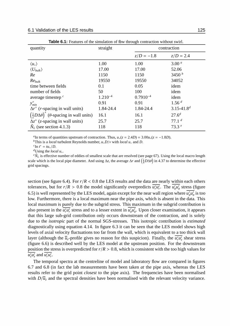
6.1 Validation of the LES results 125
Table 6.1: Features of the simulation of flow through contraction without swirl.
quantity straight contraction
z/D = −1.8 z/D = 2.4
〈u∗〉 1.00 1.00 3.00 a
〈Ubulk〉 17.00 17.00 52.06Re 1150 1150 3450 b
Rebulk 19550 19550 34052time between fields 0.1 0.05 idemnumber of fields 50 100 idemaverage timestep c 1.210−4 0.7910−4 idemy+min 0.91 0.91 1.56 d
∆r+ (r-spacing in wall units) 1.84-24.4 1.84-24.4 3.15-41.8d(
12 D∆θ
)+(θ-spacing in wall units) 16.1 16.1 27.6d
∆z+ (z-spacing in wall units) 25.7 25.7 77.1 d
NL (see section 4.1.3) 118 118 73.3 e
aIn terms of quantities upstream of contraction. Thus, u∗(z = 2.4D) = 3.00u∗(z = −1.8D).bThis is a local turbulent Reynolds number, u∗D/ν with local u∗ and D.cIn t∗ = tu∗/D.dUsing the local u∗.eNL is effective number of eddies of smallest scale that are resolved (see page 67). Using the local macro length
scale which is the local pipe diameter. And using ∆z, the average ∆r and(
14 D∆θ
)in 4.37 to determine the effective
grid spacings.
section (see figure 6.4). For r/R < 0.8 the LES results and the data are nearly within each otherstolerances, but for r/R > 0.8 the model significantly overpredicts u′ru′r. The u′
θu′θ
stress (figure6.5) is well represented by the LES model, again except for the near wall region where u′
θu′θ
is toolow. Furthermore, there is a local maximum near the pipe axis, which is absent in the data. Thislocal maximum is purely due to the subgrid stress. This maximum in the subgrid contribution isalso present in the u′ru′r stress and to a lesser extent in u′
θu′θ. Upon closer examination, it appears
that this large sub-grid contribution only occurs downstream of the contraction, and is solelydue to the isotropic part of the normal SGS-stresses. This isotropic contribution is estimateddiagnostically using equation 4.14. In figure 6.3 it can be seen that the LES model shows highlevels of axial velocity fluctuations too far from the wall, which is equivalent to a too thick walllayer (although the uz-profile gives no reason for this suspicion). Finally, the u′ru′z shear stress(figure 6.6) is described well by the LES model at the upstream position. For the downstreamposition the stress is overpredicted for r/R > 0.8, which is consistent with the too high values foru′zu′z and u′ru′r.
The temporal spectra at the centreline of model and laboratory flow are compared in figures6.7 and 6.8 (in fact the lab measurements have been taken at the pipe axis, whereas the LESresults refer to the grid point closest to the pipe axis). The frequencies have been normalisedwith D/uz and the spectral densities have been normalised with the relevant velocity variance.

126 Results of numerical simulations
LES
LDA
r/R
u z
10.80.60.40.20
25
20
15
10
5
0
r/R
u z
10.80.60.40.20
25
20
15
10
5
0
Figure 6.1: Mean axial velocity at z = −1.8D (left) and z = 2.4D (right) for flow without swirl. Thevelocities have been scaled with the local friction velocity. The radial position has beennormalised with the local pipe radius.
The experimental data suggest a very short inertial subrange for the ur-spectra and uz-spectra.This limited inertial subrange is due to the low Reynolds number. The LES spectra also show ashort inertial subrange. Furthermore, the LES-spectra fall off for higher frequencies much morerapidly than the experimental spectra, due to the dissipation of the sub-grid model. As a resultthe spectral values at lower frequencies are somewhat higher. Downstream of the contraction theLES spectra have a steeper slope than the experimental spectra (which again have a somewhatlonger inertial subrange than the LES results). This shift of energy to lower frequencies is anindication of a growth of the axial length scales (see section 2.3.2 and 2.4.2). The LES resultsshow more clearly than the experimental data that the time scale for uz becomes smaller than thatfor ur: the peak in the spectrum occurs at f Dlocal/uz = 0.4 and 0.12, respectively (see also 5.3.2).
6.1.3 Flow with swirl and axial strainTable 6.2 summarises the features of the simulation of the swirling flow. Before discussing theresults of the simulation with swirl, some features of the simulation will be discussed.
• In the simulation without swirl it was found that fields became statistically independentwell within 0.1 t∗. Therefore, the sampling interval for fields was lowered to 0.05 for thestraight pipe model, and 0.025 for the contraction model (which is computationally muchmore expensive).
• For the simulation with swirl the average time step is smaller than for the simulation withoutswirl.
The first notable difference with the flow without swirl is that the bulk velocity is 12% lower.Apparently, the swirl introduces extra friction resulting in a lower bulk velocity at a given axial

6.1 Validation of the LES results 127
LES
data
y+
u+
1000100101
25
20
15
10
5
0
y+u+
1000100101
25
20
15
10
5
0
Figure 6.2: Mean axial velocity at z = −1.8D (left) and z = 2.4D (right) for flow without swirl plottedin wall coordinates. The wall coordinates have be calculated with the local friction velocity..
LES: subgrid
LES
LDA
r/R
u z′u
z′
10.80.60.40.20
12
10
8
6
4
2
0
r/R
u z′u
z′
10.80.60.40.20
12
10
8
6
4
2
0
Figure 6.3: Comparison of LES-results to laboratory data for flow without swirl: u ′zu′z at z = −1.8D (left)and z = 2.4D (right). For further information, see figure 6.4.
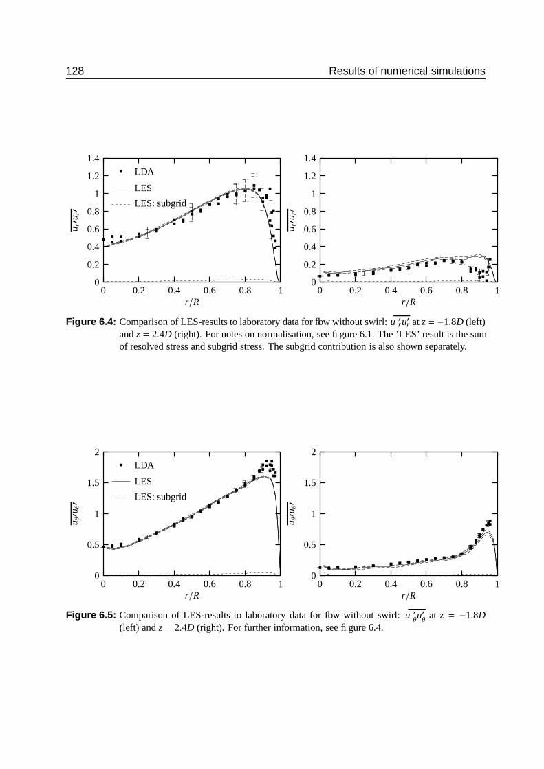
128 Results of numerical simulations
LES: subgrid
LES
LDA
r/R
u r′u
r′
10.80.60.40.20
1.4
1.2
1
0.8
0.6
0.4
0.2
0
r/Ru r′u
r′10.80.60.40.20
1.4
1.2
1
0.8
0.6
0.4
0.2
0
Figure 6.4: Comparison of LES-results to laboratory data for flow without swirl: u ′ru′r at z = −1.8D (left)and z = 2.4D (right). For notes on normalisation, see figure 6.1. The ’LES’ result is the sumof resolved stress and subgrid stress. The subgrid contribution is also shown separately.
LES: subgrid
LES
LDA
r/R
u θ′u
θ′
10.80.60.40.20
2
1.5
1
0.5
0
r/R
u θ′u
θ′
10.80.60.40.20
2
1.5
1
0.5
0
Figure 6.5: Comparison of LES-results to laboratory data for flow without swirl: u ′θu′θ
at z = −1.8D(left) and z = 2.4D (right). For further information, see figure 6.4.

6.1 Validation of the LES results 129
LES: subgrid
LES
LDA
r/R
u r′u
z′
10.80.60.40.20
1
0.8
0.6
0.4
0.2
0
r/Ru r′u
z′10.80.60.40.20
1
0.8
0.6
0.4
0.2
0
Figure 6.6: Comparison of LES-results to laboratory data for flow without swirl: u ′ru′z at z = −1.8D (left)and z = 2.4D (right). For further information, see figure 6.4.
LES
data
f Dlocal/uz
Szz/u′ zu′ z
1001010.10.01
1
0.1
0.01
0.001
LES
data
f Dlocal/uz
Szz/u′ zu′ z
1001010.10.01
1
0.1
0.01
0.001
Figure 6.7: Comparison of LES-results to laboratory data for flow without swirl: Temporal power spec-tra of uz at/near the pipe axis (r/R = 0 for lab measurements, r/R = 0.021 for LES) atz = −1.8D (left) and z = 2.4D (right). Also shown is the inertial subrange slope.
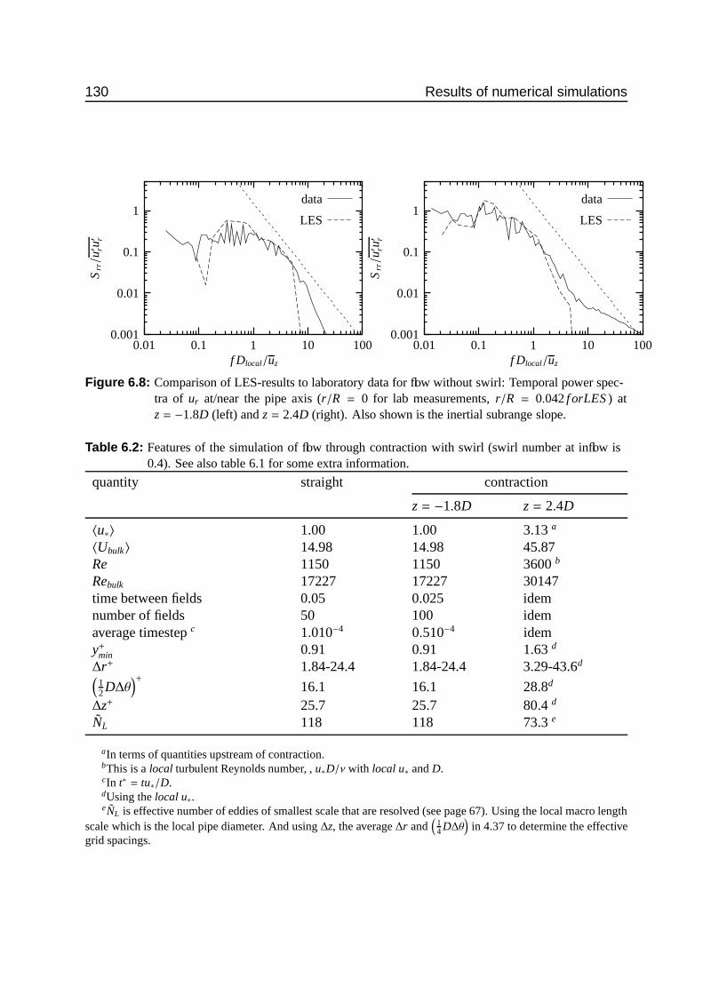
130 Results of numerical simulations
LES
data
f Dlocal/uz
Srr/u′ ru′ r
1001010.10.01
1
0.1
0.01
0.001
LES
data
f Dlocal/uz
Srr/u′ ru′ r
1001010.10.01
1
0.1
0.01
0.001
Figure 6.8: Comparison of LES-results to laboratory data for flow without swirl: Temporal power spec-tra of ur at/near the pipe axis (r/R = 0 for lab measurements, r/R = 0.042 f orLES ) atz = −1.8D (left) and z = 2.4D (right). Also shown is the inertial subrange slope.
Table 6.2: Features of the simulation of flow through contraction with swirl (swirl number at inflow is0.4). See also table 6.1 for some extra information.
quantity straight contraction
z = −1.8D z = 2.4D
〈u∗〉 1.00 1.00 3.13 a
〈Ubulk〉 14.98 14.98 45.87Re 1150 1150 3600 b
Rebulk 17227 17227 30147time between fields 0.05 0.025 idemnumber of fields 50 100 idemaverage timestep c 1.010−4 0.510−4 idemy+min 0.91 0.91 1.63 d
∆r+ 1.84-24.4 1.84-24.4 3.29-43.6d(
12 D∆θ
)+16.1 16.1 28.8d
∆z+ 25.7 25.7 80.4 d
NL 118 118 73.3 e
aIn terms of quantities upstream of contraction.bThis is a local turbulent Reynolds number, , u∗D/ν with local u∗ and D.cIn t∗ = tu∗/D.dUsing the local u∗.eNL is effective number of eddies of smallest scale that are resolved (see page 67). Using the local macro length
scale which is the local pipe diameter. And using ∆z, the average ∆r and(
14 D∆θ
)in 4.37 to determine the effective
grid spacings.

6.1 Validation of the LES results 131
forcing. Given the fact that in the simulation the Reynolds number based on u∗ is prescribed,the bulk Reynolds number is lower than for the flow without swirl. Consequently, there is a14% difference between the simulated bulk Reynolds number and the Reynolds number in thelaboratory experiment.
Figure 6.9 and 6.10 show the profiles of the mean axial velocity. Upstream of the contractionthe simulation shows a too pronounced bump near the pipe axis, whereas downstream of thecontraction the results from simulation and experiment match well, with the simulation givingslightly too low values. The small bump in the measured upstream profiles is probably the resultof the fluid that went through the central body of the swirl generator and remained isolated fromthe surrounding fluid by the strong rotation. In the simulation, however, all deviations from asmooth axial velocity profile are due to the tangential forcing.
The mean tangential velocities (figure 6.11) show a perfect agreement between experimentand simulation in the section upstream of the contraction. This agreement is of course due to thetangential forcing method used (see section 4.2.5). Downstream of the contraction, the simulatedmean tangential velocity is too low by about 20%. Analysis of the swirl number decay (figure6.43) suggests that this is due to a too high decay rate upstream of the contraction.
The results for the normal stresses are given figures 6.12 to 6.14. The general tendency for thenormal stresses is that the simulation overestimates the normal stresses throughout the pipe cross-section, except for u′ru′r, at z = −1.8D, where the overestimation is restricted to the vortex core.A plausible cause for this mismatch –given to reasonanle match of the mean velocities– is thefact that the experimental data have been multiplied with the bulk velocity from the simulation toobtain scaling with u∗. Thus any error in Ubulk/u∗ in the simulation is translated into a differencein the scaling between simulation results and experimental results. Since no experimental u∗data are available, the LDA data can not be normalised with the real u∗ to check this assertion.Another point to note is that u′ru′r and u′
θu′θ
are not equal at the centre line whereas they shouldbe. Apparently, u′
θu′θ
suffers from fluctuations (wiggles) due to the small tangential grid spacingin the centre (in the non-swirling case there was also a cusp for z/D = 2.4 but that was due to theSGS-term).
Finally, the results for the shear stresses will be discussed (see figures 6.15 to 6.17). TheLES results for the u′ru′z stress do not show the negative values in the vortex core as given bythe experimental data. Instead, the u′ru′z-profile is very similar to the straight profile in a non-swirling flow. Apparently, the u′ru′z-stress is mainly determined by the axial forcing which waskept independent of r, as in the case of the non-swirling flow. The profile for z = 2.4D showsa similar deviation of u′ru′z from the experimental data. The simulation results for u′ru
′θ
showqualitative agreement with the data, at both axial positions. At z = −1.8D the LES results are toohigh, which seems consistent with the results for the normal stresses. At z = 2.4D the tolerancesare so large that data are within the tolerance interval of the LES results for a large part of thecross-section. But the simulation results themselves (i.e. the central line of the three LES-lines)do correspond quite well with the data for r < 0.25R (near zero shear stress) and r > 0.8R(transport of tangential momentum toward the wall). The simulation results for the u′zu
′θ-stress
show qualitative agreement with the data for z = −1.8D but even quantitative agreement for thestation downstream of the contraction. For the upstream station only the profile in the vortex

132 Results of numerical simulations
LES
LDA
r/R
u z
10.80.60.40.20
25
20
15
10
5
0
r/R
u z
10.80.60.40.20
25
20
15
10
5
0
Figure 6.9: Mean axial velocity at z = −1.8D (left) and z = 2.4D (right) for flow with swirl. Thevelocities have been scaled with the local wall shear stress. The radial position has beennormalised with the local pipe radius.
core is not represented correctly.From the results for z = −1.8D it can be concluded that the tangential forcing method is
able to produce a swirling flow that qualitatively mimics the flow to be simulated. However, thedetails of the profiles of the mean axial velocity profile, as well as the shear stresses, are notcorrect. Especially, the negative value for u′ru′z for r/R < 0.5 is not represented in the simulation.It is not surprising that there is disagreement between model and data with respect to the detailsof the flow in the core. Since those details originate from the region directly downstream of theswirl generator, they can not be reproduced by a forcing that is local and axially homogeneous.
Another point to note is that the tolerance intervals for the swirling flow are larger than forthe flow without swirl. This is mainly due to the increased integral time scales in the vortex coreand an increase in the variance levels of the variable under consideration (see equation (A.12)).Especially for the statistics at z = 2.4D the tolerances for the shear stresses become very large.The choice to reduce the sampling interval relative to the non-swirling flow has been counter-productive in this sense.
Figures 6.18 and 6.19 show a comparison between data and simulation results for the temporalpower spectra for r = 0 (in fact the lab measurements have been taken at the pipe axis, whereasthe LES results refer to the grid point closest to the pipe axis). For all velocity componentsand both axial positions the agreement is remarkable. The LES spectra correctly show the shifttoward larger scales for the ur and uθ spectra (when compared to the flow without swirl). Theshift to larger scales is much more pronounced in ur than in uz (see also section 5.3.2).
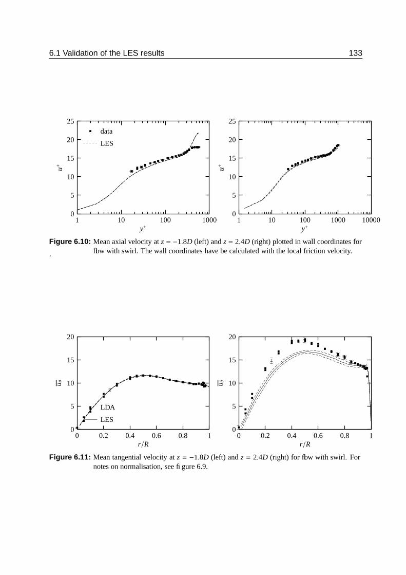
6.1 Validation of the LES results 133
LES
data
y+
u+
1000100101
25
20
15
10
5
0
y+u+
100001000100101
25
20
15
10
5
0
Figure 6.10: Mean axial velocity at z = −1.8D (left) and z = 2.4D (right) plotted in wall coordinates forflow with swirl. The wall coordinates have be calculated with the local friction velocity..
LES
LDA
r/R
u θ
10.80.60.40.20
20
15
10
5
0
r/R
u θ
10.80.60.40.20
20
15
10
5
0
Figure 6.11: Mean tangential velocity at z = −1.8D (left) and z = 2.4D (right) for flow with swirl. Fornotes on normalisation, see figure 6.9.
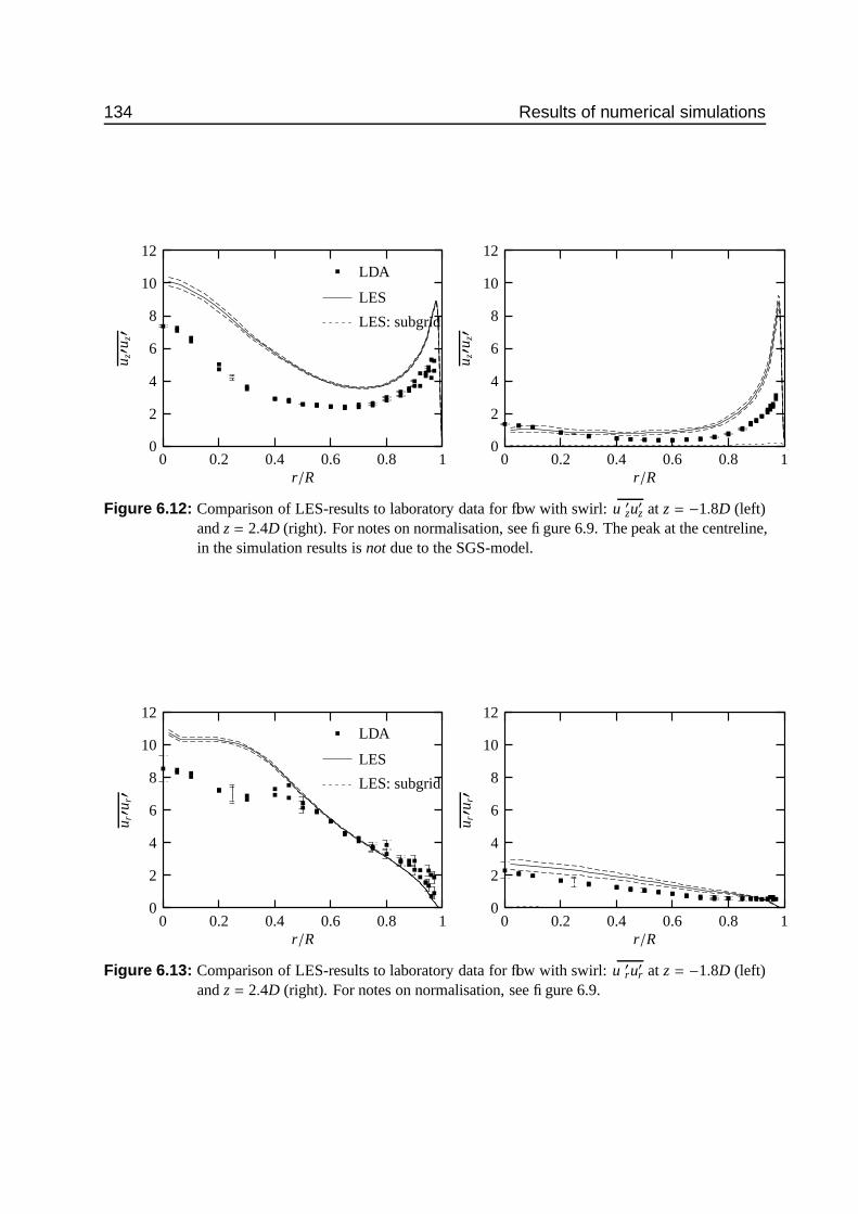
134 Results of numerical simulations
LES: subgrid
LES
LDA
r/R
u z′u
z′
10.80.60.40.20
12
10
8
6
4
2
0
r/Ru z′u
z′10.80.60.40.20
12
10
8
6
4
2
0
Figure 6.12: Comparison of LES-results to laboratory data for flow with swirl: u ′zu′z at z = −1.8D (left)and z = 2.4D (right). For notes on normalisation, see figure 6.9. The peak at the centreline,in the simulation results is not due to the SGS-model.
LES: subgrid
LES
LDA
r/R
u r′u
r′
10.80.60.40.20
12
10
8
6
4
2
0
r/R
u r′u
r′
10.80.60.40.20
12
10
8
6
4
2
0
Figure 6.13: Comparison of LES-results to laboratory data for flow with swirl: u ′ru′r at z = −1.8D (left)and z = 2.4D (right). For notes on normalisation, see figure 6.9.
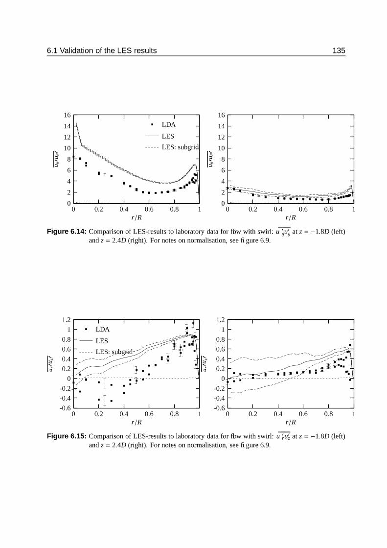
6.1 Validation of the LES results 135
LES: subgrid
LES
LDA
r/R
u θ′u
θ′
10.80.60.40.20
16
14
12
10
8
6
4
2
0
r/Ru θ′u
θ′
10.80.60.40.20
16
14
12
10
8
6
4
2
0
Figure 6.14: Comparison of LES-results to laboratory data for flow with swirl: u ′θu′θ
at z = −1.8D (left)and z = 2.4D (right). For notes on normalisation, see figure 6.9.
LES: subgrid
LES
LDA
r/R
u r′u
z′
10.80.60.40.20
1.2
1
0.8
0.6
0.4
0.2
0
-0.2
-0.4
-0.6
r/R
u r′u
z′
10.80.60.40.20
1.2
1
0.8
0.6
0.4
0.2
0
-0.2
-0.4
-0.6
Figure 6.15: Comparison of LES-results to laboratory data for flow with swirl: u ′ru′z at z = −1.8D (left)and z = 2.4D (right). For notes on normalisation, see figure 6.9.
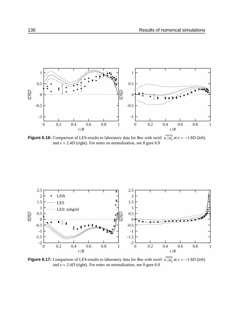
136 Results of numerical simulations
r/R
u r′u
θ′
10.80.60.40.20
1
0.5
0
-0.5
-1
r/R
u r′u
θ′
10.80.60.40.20
1
0.5
0
-0.5
-1
Figure 6.16: Comparison of LES-results to laboratory data for flow with swirl: u ′ru′θ at z = −1.8D (left)and z = 2.4D (right). For notes on normalisation, see figure 6.9
LES: subgrid
LES
LDA
r/R
u θ′u
z′
10.80.60.40.20
2.5
2
1.5
1
0.5
0
-0.5
-1
-1.5
-2
r/R
u θ′u
z′
10.80.60.40.20
2.5
2
1.5
1
0.5
0
-0.5
-1
-1.5
-2
Figure 6.17: Comparison of LES-results to laboratory data for flow with swirl: u ′zu′θ at z = −1.8D (left)and z = 2.4D (right). For notes on normalisation, see figure 6.9

6.1 Validation of the LES results 137
LES
data
f Dlocal/uz
Szz/u′ zu′ z
1001010.10.01
1
0.1
0.01
0.001
LES
data
f Dlocal/uz
Szz/u′ zu′ z
1001010.10.01
1
0.1
0.01
0.001
Figure 6.18: Comparison of LES-results to laboratory data for flow with swirl: Temporal power spectraof uz at/near the pipe axis (r/R = 0 for lab measurements, r/R = 0.021 f orLES ) at z =−1.8D (left) and z = 2.4D (right). Also shown is the inertial subrange slope.
LES
data
f Dlocal/uz
Srr/u′ ru′ r
1001010.10.01
1
0.1
0.01
0.001
LES
data
f Dlocal/uz
Srr/u′ ru′ r
1001010.10.01
1
0.1
0.01
0.001
Figure 6.19: Comparison of LES-results to laboratory data for flow with swirl: Temporal power spectraof ur at/near the pipe axis (r/R = 0 for lab measurements, r/R = 0.042 f orLES ) at z =−1.8D (left) and z = 2.4D (right). Also shown is the inertial subrange slope.

138 Results of numerical simulations
6.2 Further analysis of LES resultsIn this section the results of the simulations will be analysed further. First the spatial patterns inthe fields of mean velocity and turbulent stress will be discussed (section 6.2.1). Subsequentlythe terms of the stress budgets will be dealt with (section 6.2.2). For the locations and quantitiesanalysed here, no experimental data is available, so that the simulation results will be presentedwithout validation with experimental data.
6.2.1 Velocity and stress fieldsBefore presenting the results, first a few remarks with respect to the presentation of those resultsare in place:
• The fields of mean velocity and turbulent stresses are presented as grey-scale plots.• The mean velocities have been normalised with the local bulk velocity, because the down-
stream development of the mean velocities is mainly determined by the axial acceleration.Any details of the downstream development would be lost if this acceleration would not beremoved by scaling.
• The stresses have been scaled with the u∗2 at the inlet as in the model. In this way thedownstream development of the stresses is most apparent. Furthermore, a direct relationshipbetween a turbulent stress and the wall shear stress at a given axial location is not expected.
• The values that correspond to the minimum and maximum grey-scale have been chosensuch that structure of the fields is as clear as possible (i.e. the data have been clipped).
Flow without swirlFigure 6.20 shows the fields of the mean velocities and turbulent stresses. The main conclusionthat can be drawn from the figures for ur and uz is that the upstream influence of the contractionon the mean flow is limited to z/D > −0.5. Furthermore, ur is appreciably non-zero only betweenfor −0.5 < z/D < 1. Further downstream, however, ur can not be zero exactly, since the axialvelocity still develops (mass conservation implies that if ∂
∂zuz , 0 then also ∂∂r rur , 0). The
axial acceleration inside the contraction mainly takes place directly at the start of the change indiameter (z/D ≈ 0).
The figure for u′ru′r shows that at the downstream edge of the contraction u′ru′r increases sharply.Further downstream (down to z ≈ 1.5D) the levels of u′ru′r decrease again. Downstream ofz ≈ 2.5D, u′ru′r starts to increase again, first close to the wall: the boundary layer grows. Thispattern explains the profile shown in figure 6.4: maxima at r/R = 0.7 and 0.9. The u′
θu′θ-stress
is strongly enhanced inside the contraction, but the resulting stress decreases downstream ofthe contraction. Then at r ≈ 1.5D the u′
θu′θ-stress starts to increase again, due to the growth
of the boundary layer. For u′zu′z the situation is different. At the entrance of the contraction asmall region of enhanced u′zu′z occurs near the wall. At the exit u′zu′z starts to increase again, anddue to the growth of the boundary later, the region of higher u′zu′z grows –apparently linearly–with downstream distance. Finally, the shear stress u′ru′z is discussed. Inside the contraction,a localised region with increased u′ru′z exists near the wall. There, the axially accelerated flowexperiences extra friction. Downstream of the contraction u′ru′z causes the boundary layer to

6.2 Further analysis of LES results 139
Figure 6.20: Mean velocity and stress fields for flow with axial strain, without swirl. From top to bot-tom: uz. ur (normalised with local Ubulk) u′zu′z, u′ru′r, u′
θu′θ
and u′ru′z (normalised with u∗ atentrance). The values have been clipped to a range that can be deduced from the scale tothe right of each picture. Clipping of the values has been done to enhance features in thepictures. The stresses include the subgrid contribution.
grow. This boundary layer growth is in turn reflected in a downstream increase of the regionwith larger u′ru′z.
An important conclusion that can be drawn from figure 6.20 is that upstream of the contractionthe stresses are hardly affected by the presence of the contraction. Only for u′zu′z a slight changecan be discerned for −0.2 < z/D < 0. Furthermore, the figure does not show any change in thedownstream development of the flow as the outflow plane is approached. This gives confidencein the treatment of the outflow boundary conditions in the model.
Flow with swirlIn figure 6.21 the fields of mean velocities and stresses for the flow with swirl are shown. Thefigures for the mean velocities uz and ur do not differ much from those for the flow without swirl.The field of uz shows that the local maximum around the pipe axis has nearly disappeared atz/D = 0. Further downstream, the region of high uz inside the contraction is larger than for the

140 Results of numerical simulations
Figure 6.21: Mean velocity and stress fields for flow with axial strain, with swirl. From top to bottom:uz. ur, uθ (normalised with local Ubulk) u′zu′z, u′ru′r, u′
θu′θ, u′ru′z, u′ru′θ and u′zu′θ (normalised
with u∗ at entrance). The values have been clipped to a range that can be deduced from thescale to the right of each picture. Clipping of the values has been done to enhance featuresin the pictures. The stresses include the subgrid contribution.

6.2 Further analysis of LES results 141
flow without swirl. Downsteam of the contraction, the axial development of the uz-profile seemsto be slower than for the flow without swirl.
In the figure for uθ, the decay of swirl is hardly visible, due to the fact that the main changein uθ is due to the fact that uθ ∼ D−1 whereas the velocities have been scaled with the local bulkvelocity, which scales as Ubulk ∼ D−2. Furthermore, inside the contraction the vortex core isreduced in size, although the size relative to the pipe diameter remains the same (see also figure5.12).
The three normal stresses, upstream of the contraction, exhibit enhanced values around thecentre line. The possible origins of these higher variance was discussed in section 5.2. Theeffect of the contraction is that u′ru′r and u′
θu′θ
are further increased, whereas u′zu′z is diminished, inaccordance with the experimental data and with RDT (section 5.2.5). The peak of u′ru′r and u′
θu′θ
around the centre remains throughout the model domain for z > 0. The downstream developmentof the normal stresses is not easily compared between flows without and with swirl due to thelarge difference in shape of the profiles of those stresses (see figures 5.2 and 5.7 for the full axialdevelopment).
The u′ru′z shear stress shows an increase within the contraction, less localised than for thenon-swirling flow. In a thin layer close to the wall in the contraction u′ru′z is less than zero.This is due to the fact that flow is oblique to the directions of the r-velocity and z-velocitycomponents: velocity fluctuations parallel to the wall will yield negative correlation between uz
and ur. Directly downstream of the contraction u′ru′z is zero in most of the pipe cross-section.But the layer, adjacent to the wall, where u′ru′z is positive, grows rapidly downstream. If theshear stress u′ru′z is used as an indicator of the growth of the boundary layer, the rate of growthappears to be larger for the swirling flow than for the non-swirling flow. This is in accordancewith the destabilising effect of concave curvature on a shear flow (see section 2.2.2). For u′ru
′θ
the field is similar as for u′ru′z. Upstream of the contraction there is transport of θ-momentumtoward the wall, and some transport toward the pipe centre in the vortex core. Downstream ofthe contraction u′ru
′θ
is negative around the pipe centre. The region of positive u′ru′θ
near the wallgrows downstream at the same pace as the region of positive u′ru′z. Inside the contraction, there isa positive u′ru
′θ
near the wall (i.e. loss of θ-momentum due to friction). Finally, the field of u′zu′θ
is discussed. This stress is negative or near zero around the pipe centre over the total length ofthe domain. Upstream of the contraction a thin layer with large positive values exists close to thewall. Downstream of the contraction this layer starts to grow, but for z > 2D a fuzzy transitionlayer starts to develop between the negative values near the pipe axis and the positive values nearthe wall. The growth of the layer with positive u′zu
′θ
is different in nature than the growth of theu′ru′z boundary layer: due to swirl decay the angle between the velocity and the axial directiondecreases and consequently u′zu
′θ
deceases. The vortex core appears immune to swirl decay andthus u′zu
′θ
remains virtually constant there.
6.2.2 Budgets for turbulent stressesTo understand the dynamics of the Reynolds stresses, the terms of the conservation equations forthose stresses (the budget terms) need to be computed. Whereas this is (nearly) impossible todo with experimental data, from LES fields the budget terms can readily be computed. In this

142 Results of numerical simulations
section the budget terms are presented in two ways: as profiles for the axial positions z/D = −1.8and 2.4, and as fields (grey-scale pictures) for the entire model domain.
Before discussing the results of the budget terms, first some remarks will be made regardingthe computation and presentation of those terms.
• The budget equations can be found in section B.1.2.• The budget terms have not been computed using the analytical equations in B.1.2. Rather,
the computation is based on the procedure used in the derivation of the budget equations:multiplication of the (discretized) conservation equation for uuu′ with uuu′ (see Stull (1988) forthe procedure, Gao et al. (1994) for the application to LES results).
• No attempt has been made to split the pressure-gradient velocity terms into pressure-strainand pressure-diffusion terms (see appendix H for a study of the pressure strain terms in arotating pipe). Neither has the viscous term been split into viscous dissipation and viscousdiffusion. Finally, no distinction is made between the effect of molecular viscosity and thesub-grid scale viscosity. So subgrid and molecular diffusion have been added.
• For the profiles of budget terms shown in this section, the data for z = −1.8D have beendeduced from the fields of the straight pipe model. The data for z = 2.4D have beencomputed with the fields from the contraction model.
• In the presentation of the profiles of budget terms, for the radial coordinate the distance tothe wall in viscous units is used, indicated by y+ (= yu∗/ν). At both axial a local u∗ has beenused to determine y+ Furthermore, the budget terms themselves have also been scale withthe local u∗2. Where feasible, the profiles at both axial locations have been plotted with thesame vertical scale.
• In the profiles of the budget terms, the sum of those terms is also shown. This sum shouldbe zero if the budget is balanced exactly.
• The fields of the budget terms have been scaled differently: there the budget terns have beenscaled with the local value of the stress under consideration. In that way, the fields will showthe relative gain or loss due to a certain term. Consequently, the effects of large differencesin the values of the stress on their budget terms are eliminated.
Flow with axial strainFigures 6.22 to 6.29 show the profiles of the budget terms for z = −1.8D and z = 2.4D, as wellas the fields of those terms throughout the model domain. The first conclusion that can be drawnfrom the profiles is that there is hardly any difference in the shape of the profiles between the twoaxial locations, except for the fact that the budget terms are nearly zero for y+ > 90 for z = 2.4D.Furthermore, there is some change in the relative size of the various terms. The scaling with thelocal u∗ appears to be appropriate, given that for most stresses (except u′ru′z and u′zu′z) the budgetterms have equal orders of magnitude at both axial locations.
Another important conclusion is that the sum of all budget terms is very small (relative to theactual budget terms) for all budgets. This indicates that method of used in the determination ofthe budget terms is accurate.
The budget for u′zu′z does not differ much between both axial positions (figure 6.22). Thebudget terms are an order of magnitude larger at z/D = 2.4 than at the upstream location (due

6.2 Further analysis of LES results 143
y+
term
sin
budg
etof
u′ zu′ z
1000100101
600
400
200
0
-200
-400
-600
sumDS+VD
VPCTPRTD
y+te
rms
inbu
dget
ofu′ zu′ z
1000100101
2500
2000
1500
1000
500
0
-500
-1000
-1500
-2000
-2500
Figure 6.22: Budget terms for u′zu′z-budget. For flow without swirl at z/D = −1.8 and z/D = 2.4.
Figure 6.23: Terms in the budget of u′zu′z for flow with axial strain, without swirl. From top to bottom:TD (turbulent diffusion), PR (production), CT (convective transport), VP (velocity-pressuregradient correlation term), DS+VD (dissipation + viscous diffusion). The values of thebudgets have been normalised with the local value of the stress under consideration, so thatthe scaled budget terms indicate the relative change in the given stress. The values of thebudget have been clipped in order to highlight the structure of the fields. The pipe wall isindicated with a fine black line. The horizontal axis gives the axial position z/D where Dis the upstream pipe diameter.

144 Results of numerical simulations
sumDS+VDVPCTPRTD
y+
term
sin
budg
etof
u′ ru′ r
1000100101
50
40
30
20
10
0
-10
-20
-30
y+te
rms
inbu
dget
ofu′ ru
′ r1000100101
50
40
30
20
10
0
-10
-20
-30
Figure 6.24: Budget terms for u′ru′r-budget. For flow without swirl at z/D = −1.8 and z/D = 2.4. Fornotes on the normalisation: see the text.
Figure 6.25: Terms in the budget of u′ru′r (normalised with the local u′ru′r) for flow with axial strain,without swirl. For more details, see figure 6.23).

6.2 Further analysis of LES results 145
y+
term
sin
budg
etof
u′ θu′ θ
1000100101
150
100
50
0
-50
-100
-150sum
DS+VDVPCTPRTD
y+te
rms
inbu
dget
ofu′ θ
u′ θ1000100101
150
100
50
0
-50
-100
-150
Figure 6.26: Budget terms for u′θu′θ-budget. For flow without swirl at z/D = −1.8 and z/D = 2.4. From
top to bottom: TD, PR, CT, VP, and DS+VD.
Figure 6.27: Terms in the budget of u′θu′θ
(normalised with the local u′θu′θ) for flow with axial strain,
without swirl. From top to bottom: TD, PR, CT, VP, and DS+VD. For more details, seefigure 6.23).
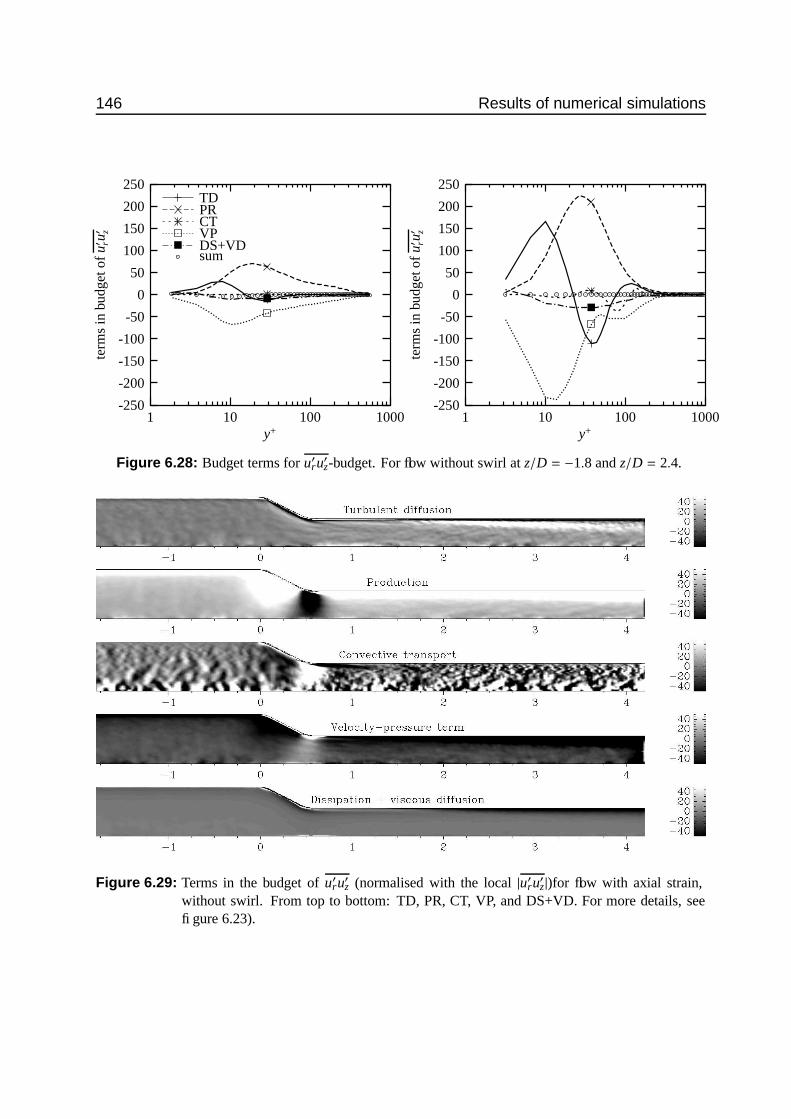
146 Results of numerical simulations
sumDS+VDVPCTPRTD
y+
term
sin
budg
etof
u′ ru′ z
1000100101
250
200
150
100
50
0
-50
-100
-150
-200
-250
y+te
rms
inbu
dget
ofu′ ru′ z
1000100101
250
200
150
100
50
0
-50
-100
-150
-200
-250
Figure 6.28: Budget terms for u′ru′z-budget. For flow without swirl at z/D = −1.8 and z/D = 2.4.
Figure 6.29: Terms in the budget of u′ru′z (normalised with the local |u′ru′z|)for flow with axial strain,without swirl. From top to bottom: TD, PR, CT, VP, and DS+VD. For more details, seefigure 6.23).

6.2 Further analysis of LES results 147
to the extreme shear production). Production occurs throughout the pipe cross-section, turbulentdiffusion is a gain term close to the wall but a loss term toward the pipe axis. Dissipation is a lossterm, and the pressure-velocity term is a small but important loss term, since it feeds the energythe two other normal stresses. The pressure-velocity loss terms is relatively smaller at z/D = 2.4than at z/D = −1.8. In absolute value, however, it is larger, as can also be seen from the increedmagnitude of the gain from the VP-term for the other stresses.
From the fields of the u′zu′z-budget terms, shown in figure 6.23, it can be concluded that thebudget is roughly identical both upstream and downstream of the contraction, except for the orderof magnitude of the terms. Inside the contraction, however, negative production occurs, whereasconvective transport is a major gain term. Furthermore, the radial transport (away from the wall)by turbulent diffusion is stronger than outside the contraction.
For u′ru′r the main change between the two axial positions, is that at z = 2.4D the velocity-pressure correlations and the turbulent diffusion have increased, relative to the dissipation term.For both locations u′ru′r gains near the wall, due to turbulent diffusion, whereas further towardthe pipe axis, turbulent diffusion is a loss term. Note the large fluctuations at z = 2.4D in theconvective transport (CT) term. This is due to statistical errors in the stresses. CT is proportionalto the mean velocity in given direction and the gradient of a stress in the same direction. Espe-cially in the axial direction (with a large mean velocity and some statistical error in the stresses)this gives rise to large statistical errors in the budget term. This feature will occur in all budgetsderived from fields from the contraction model.
The fields of the u′ru′r-budget terms are shown in figure 6.25. As was already clear from thespatial patterns of the stresses, there are two important regions. One is inside the contraction,where u′ru′r is produced, and subsequently lost by convective transport. There is also some neg-ative production at the trailing edge of the contraction. Furthermore, there is a streak, startinginside the contraction and extending to z = 1.5D where the pressure-velocity term feeds the u′ru′rstress and turbulent diffusion is a loss term. Convective transport appears to be a gain term aswell, although the noise is rather large. The second region of interest starts at z = 2D. Hereagain, there is a balance between the pressure-velocity term and dissipation, with turbulent dif-fusion acting as a spatial redistributor (see also figure 6.24).
The budget for u′θu′θ
is rather simple. It is a balance between the pressure-velocity correlationterm and dissipation. This is the same for both axial positions. From the fields of the budgetterms (figure 6.27) the following observations can be made. This budget is, near the wall, mainlya balance between the pressure-velocity term (gain) and dissipation (loss). At the trailing edgeof the contraction convective transport is a gain and the pressure-velocity term is –locally– a lossterm. Furthermore, in the contraction and just downstream of it, there is some spatial redistribu-tion by turbulent diffusion (transport away from the wall).
In the u′ru′z-stress budget the main difference between the two axial positions is that the am-plitude of the turbulent diffusion term becomes relatively large downstream of the contraction:a gain term near the wall and a loss term toward the pipe axis. In general, the magnitude ofthe budget terms has increased at the downstream location. The shear stress is fed through theproduction term and is mainly drained by the pressure-velocity term. Dissipation is only a minorterm in this budget. From the fields of the budget terms (figure 6.29) it can be seen that thebudget terms exhibit the same profiles over the entire length of the domain, except inside and

148 Results of numerical simulations
directly downstream of the contraction. Inside, there is positive production and negative con-vective transport, whereas, at the trailing edge of the contraction, the gain due to the convectivetransport term and the pressure-velocity term is balanced by a negative production term.
Flow with axial strain and swirl
In figures 6.30 to 6.41 the profiles of the budget terms at z = −1.8D and z = 2.4D, as well as thefields of those terms are shown for the case with swirl.
From the profiles a difference with the non-swirling flow is immediately clear: whereas inthe non-swirling flow the terms are nearly zero close to the pipe axis, they are large (and evendominate over the near-wall values) near the pipe axis.
The budget for u′zu′z (figures 6.30 and 6.31) is very similar to the budget for the flow withoutswirl. Upstream of the contraction the only difference is the occurrence of high levels of thedissipation and pressure-velocity terms near the pipe axis. Although this cusp seems unrealistic,the fact that it is not restricted to the first gridpoint off the pipe axis suggests that it is a realphenomenon. From the fields in 6.31 one can see that there are more places in the domain wherepatches of high, positive, values of the pressure-velocity occur. At z = 2.4D the only visibledifference is the fact that, in the wall region, the production is somewhat higher for the swirlingflow, and that the turbulent diffusion term is smaller. Any influence of the vortex core is no longervisible. The fields of the budget terms (figure 6.31) show some more differences. In general,there is more scatter in the fields than for the flow without swirl. The negative production insidethe contraction is similar to that for the flow without swirl. The pattern of the pressure-velocityterm differs from that for the flow without swirl. Inside the contraction, close to the wall thereis a positive contribution from VP to u′zu′z. The gain patch of positive VP that was inside thecontraction for the non-swirling flow, has shifted to a location downstream of the contraction inthe swirling flow. Furthermore, there are patches of positive VP near the pipe axis that do notexist in the flow without swirl.
The budget of u′ru′r (shown in figures 6.32 and 6.33) is dominated by the vortex core. In thatpart of the cross-section, the gain due to production, convective transport and turbulent diffusionis balanced by dissipation and the pressure-velocity term. At z = 2.4D the magnitude of the termsin the vortex core has diminished, relative to the near-wall values. For y+ < 300 the structureof the terms is more or less identical to that at z = −1.8D. Inside a part of the vortex core atz/D = 2.4 (roughly 500 < y+ < 800) a sign reversal of most terms occurs: production becomesnegative and the pressure-velocity term becomes positive. The fields, shown in figure 6.33,reveal that this region of sign reversal appears to originate at the trailing edge of the contraction.A similar structure appears in the flow without swirl (figure 6.25), but there the region thatoriginates at the trailing edge of the contraction is thinner and remains close to the wall. Exceptfor this region of sign reversal, and the high values near the pipe axis, the overall structure of thebudget terms is similar for the flows without and with swirl.
The budgets of u′θu′θ
are shown in figures 6.34 and 6.35. As in the flow without swirl, thebudget upstream of the contraction is dominated by the pressure-velocity term and dissipationwith a small role for turbulent diffusion. Near the pipe wall the same terms are important buttheir values are larger. Furthermore, the production term is strongly negative near the pipe centre.

6.2 Further analysis of LES results 149
y+
term
sin
budg
etof
u′ zu′ z
1000100101
1000
500
0
-500
-1000
sumDS+VD
VPCTPRTD
y+te
rms
inbu
dget
ofu′ zu′ z
1000100101
2500
2000
1500
1000
500
0
-500
-1000
-1500
-2000
-2500
Figure 6.30: Budget terms for u′zu′z-budget. For flow with swirl at z/D = −1.8 and z/D = 2.4.
Figure 6.31: Terms in the budget of u′zu′z for flow with axial strain, with swirl. From top to bottom: TD(turbulent diffusion), PR (production), CT (convective transport), VP (velocity-pressuregradient correlation term), DS+VD (dissipation + viscous diffusion). The values of thebudgets have been normalised with the local (absolute) value of the stress under consider-ation, so that the scaled budget terms indicate the relative change in the given stress. Thevalues of the budget have been clipped in order to highlight the structure of the fields. Thepipe wall is indicated with a fine black line.

150 Results of numerical simulations
sumDS+VDVPCTPRTD
y+
term
sin
budg
etof
u′ ru′ r
1000100101
200
150
100
50
0
-50
-100
-150
-200
y+te
rms
inbu
dget
ofu′ ru′ r
1000100101
200
150
100
50
0
-50
-100
-150
-200
Figure 6.32: Budget terms for u′ru′r-budget. For flow with swirl at z/D = −1.8 and z/D = 2.4.
Figure 6.33: Terms in the budget of u′ru′r (normalised with the local u′ru′r) for flow with axial strain, withswirl. From top to bottom: TD, PR, CT, VP, and DS+VD. For more details, see figure6.31).

6.2 Further analysis of LES results 151
y+
term
sin
budg
etof
u′ θu′ θ
1000100101
400
200
0
-200
-400 sumDS+VD
VPCTPRTD
y+te
rms
inbu
dget
ofu′ θ
u′ θ1000100101
400
200
0
-200
-400
Figure 6.34: Budget terms for u′θu′θ-budget. For flow with swirl at z/D = −1.8 and z/D = 2.4.
Figure 6.35: Terms in the budget of u′θu′θ
(normalised with the local u′θu′θ) for flow with axial strain, with
swirl. From top to bottom: TD, PR, CT, VP, and DS+VD. For more details, see figure6.31).

152 Results of numerical simulations
sumDS+VDVPCTPRTD
y+
term
sin
budg
etof
u′ ru′ z
1000100101
300
200
100
0
-100
-200
-300
y+te
rms
inbu
dget
ofu′ ru′ z
1000100101
300
200
100
0
-100
-200
-300
Figure 6.36: Budget terms for u′ru′z-budget. For flow at z/D = −1.8 and z/D = 2.4.
Figure 6.37: Terms in the budget of u′ru′z (normalised with the local |u′ru′z|) for flow with axial strain,with swirl. From top to bottom: TD, PR, CT, VP, and DS+VD. For more details, see figure6.31).

6.2 Further analysis of LES results 153
sumDS+VDVPCTPRTD
y+
term
sin
budg
etof
u′ ru′ θ
1000100101
600
400
200
0
-200
-400
-600
y+te
rms
inbu
dget
ofu′ ru
′ θ1000100101
600
400
200
0
-200
-400
-600
Figure 6.38: Budget terms for u′ru′θ-budget. For flow with swirl at z/D = −1.8 and z/D = 2.4.
Figure 6.39: Terms in the budget of u′ru′θ (normalised with the local |u′ru′θ |) for flow with axial strain,with swirl. From top to bottom: TD, PR, CT, VP, and DS+VD. For more details, see figure6.31).

154 Results of numerical simulations
y+
term
sin
budg
etof
u′ zu′ θ
1000100101
200
150
100
50
0
-50
-100
-150
-200
sumDS+VD
VPCTPRTD
y+te
rms
inbu
dget
ofu′ zu′ θ
1000100101
600
400
200
0
-200
-400
-600
Figure 6.40: Budget terms for u′zu′θ-budget. For flow with swirl at z/D = −1.8 and z/D = 2.4.
Figure 6.41: Terms in the budget of u′zu′θ (normalised with the local |u′zu′θ |) for flow with axial strain,with swirl. From top to bottom: TD, PR, CT, VP, and DS+VD. For more details, see figure6.31).

6.2 Further analysis of LES results 155
At z = 2.4D, additionally, the production term becomes important near the wall. In the fieldsshown in figure 6.35 the same structure occurs as in the budget of u′ru′r: a streak originating atthe trailing edge of the contraction and extending toward the pipe centre further downstream.This structure has nearly disappeared at z/D = 2.4. In this streak the production term is positiveand the velocity-pressure term is negative. The turbulent diffusion term tends to remove u′
θu′θ
away from the production zone. One would expect a positive production term near the pipe wall,given the shear in uθ. However, the budget at z/D = −1.8 has been derived from the simulationof the straight pipe, in which uθ was forced. The forced profile had such a steep gradient of uθnear the wall (see figure 6.11), that the production term could not be resolved. The budget atz/D = −1.8, derived from the contraction model in which uθ is not forced (not shown), indeedshows a positive production term for u′
θu′θ.
Figures 6.36 and 6.37 show the budgets of u′ru′z. Upstream of the contraction, the main dif-ference between the flow without swirl and the swirling flow occurs near the pipe axis: in theswirling flow a large production term (absent in the non-swirling case) is balanced by convectivetransport and the pressure-velocity term. Downstream of the contraction the same difference oc-curs, but the magnitude of the terms near the pipe axis is smaller relative to the near-wall values.When considering the fields of the budget terms (figure 6.37), the most striking feature is thestreak of negative production and positive pressure-velocity term that originates at the trailingedge of the contraction. This structure is also visible in the shear-stress fields (see figure 6.21).Furthermore, there is mostly positive production in the rest of the pipe cross-section (as opposedto only near-wall production in the non-swirling case).
The u′ru′θ
budget (figures 6.38 and 6.39) is dominated by high values for most terms near thepipe axis: negative production and positive convective transport and a pressure-velocity term.In the near-wall region for y+ < 100 the pressure-velocity term is a loss term and convectivetransport and production are positive. In figure 6.39 it can be seen that turbulent diffusion mainlyplays a role inside the contraction, down to z = 2D, as well as around the pipe axis. The pressurevelocity term is positive around the pipe axis, but directly downstream of the contraction theregion of positive VP is smaller as compared to upstream of the contraction and to the regionz > 1.5D. Finally, contrary to the budgets of other stresses, the convective transport term isimportant in large parts of the domain. This is due to the curvature induced terms involving uθ/r.
The budget of u′zu′θ
(figures 6.40 and 6.41) mainly shows large terms in the near-wall region.There is a complicated balance between production and turbulent diffusion (mostly positive)and dissipation and the pressure-velocity term. Close to the pipe axis there is a region wherethe pressure-velocity term is the gain term and production and turbulent diffusion are negative.Downstream of the contraction the terms are small near the pipe axis. Near the wall there is againa balance between production (positive) and pressure-velocity and dissipation. The turbulentdiffusion term is again smaller (relative to the others) than upstream of the contraction, andredistributes the stress radially. The fields of the budget terms (figures 6.41) reveal that inside thecontraction production of u′zu
′θ
occurs near the wall. Furthermore, the pressure-velocity term isa large gain term inside the contraction (except near the wall), probably due to the simultaneousoccurrence of large axial pressure gradient fluctuations and large fluctuations in uθ.

156 Results of numerical simulations
arr/k, dataazz/k, dataarr/k, LESazz/k, LES
arr/k, RDTazz/k, RDT
z/D
anis
otro
py
43210-1-2
0.8
0.6
0.4
0.2
0
-0.2
-0.4
arr/k, dataazz/k, dataarr/k, LESazz/k, LES
arr/k, RDTazz/k, RDT
z/D
anis
otro
py
43210-1-2
0.8
0.6
0.4
0.2
0
-0.2
-0.4
Figure 6.42: Stress anisotropy on the centre line: comparison between LES results, RDT and experi-mental data. Flow without swirl (left) and with swirl (right). LES and experimental resultsrefer to a Rebulk = 2 · 104.
6.2.3 Stress anisotropy at the pipe axisAnalogously to the analysis in section 5.2.5, the axial development of the stress anisotropy at thepipe axis will be studied. Since in the model none of the stresses are available at the centreline,the centreline value is obtained by extrapolation of the radial profiles. To this end, quadraticextrapolation was used. The resulting axial profiles are shown in figure 6.42 for the flow withoutand with swirl. Apart from the LES results, also the RDT predictions (starting at z = 0) and theexperimental data are shown. Note that the apparently random variation of the anisotropies inthe LES results is due to the very limited number of independent samples available (see appendixA).
For the non-swirling flow, the anisotropies at the entrance of the domain compare well withthe experimental data. Between z = −1.8D and the entrance of the contraction, the anisotropydecreases somewhat. As a result, the starting values for the RDT analysis are too high, since thosevalues were based on observations at z = −1.8D (and for Rebulk = 105). As a consequence of theincorrect value for the anisotropies at z = 0, the values at the end of the contraction are incorrectas well. However, there is a close correspondence between the change in the anisotropies, withinthe contraction, as given by the LES and as predicted by RDT. At z = 2.4D the LES results showa higher anisotropy than both the observations and the RDT analysis. The LES results suggestthat only downstream of z = 2.5D the anisotropies start to diminish gradually.
For the swirling flow both the experimental data and the LES results show a smaller stressanisotropy upstream of the contraction. The change in anisotropy between z = −1.8D and theentrance of the contraction is small. Consequently, the starting values for the RDT analysis cor-respond to both the experimental values and the LES results. The agreement between LES resultsand RDT analysis in the development of the anisotropy within the contraction is striking. How-ever, downstream of the contraction, the RDT analysis (which is no longer valid there) predicts
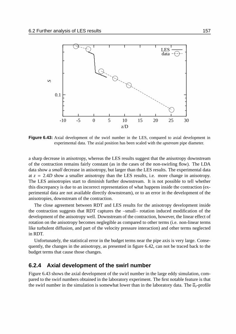
6.2 Further analysis of LES results 157
dataLES
z/D
S
302520151050-5-10
0.1
Figure 6.43: Axial development of the swirl number in the LES, compared to axial development inexperimental data. The axial position has been scaled with the upstream pipe diameter.
a sharp decrease in anisotropy, whereas the LES results suggest that the anisotropy downstreamof the contraction remains fairly constant (as in the cases of the non-swirling flow). The LDAdata show a small decrease in anisotropy, but larger than the LES results. The experimental dataat z = 2.4D show a smaller anisotropy than the LES results, i.e. more change in anisotropy.The LES anisotropies start to diminish further downstream. It is not possible to tell whetherthis discrepancy is due to an incorrect representation of what happens inside the contraction (ex-perimental data are not available directly downstream), or to an error in the development of theanisotropies, downstream of the contraction.
The close agreement between RDT and LES results for the anisotropy development insidethe contraction suggests that RDT captures the –small– rotation induced modification of thedevelopment of the anisotropy well. Downstream of the contraction, however, the linear effect ofrotation on the anisotropy becomes neglegible as compared to other terms (i.e. non-linear termslike turbulent diffusion, and part of the velocity pressure interaction) and other terms neglectedin RDT.
Unfortunately, the statistical error in the budget terms near the pipe axis is very large. Conse-quently, the changes in the anisotropy, as presented in figure 6.42, can not be traced back to thebudget terms that cause those changes.
6.2.4 Axial development of the swirl numberFigure 6.43 shows the axial development of the swirl number in the large eddy simulation, com-pared to the swirl numbers obtained in the laboratory experiment. The first notable feature is thatthe swirl number in the simulation is somewhat lower than in the laboratory data. The uθ-profile

158 Results of numerical simulations
of the simulation matches the experimental data perfectly due to the forcing method. Therefore,the discrepancy in the swirl numbers must be attributed to the difference in the shape of the uz-profile. The simulation exhibits an exaggerated bump near the pipe centre. Consequently, uz istoo low in the region outside the vortex core, where ur is highest. This results in a lower swirlnumber (see equation (2.17)). Downstream of the contraction, the role of the two velocity com-ponents is reversed: the uz-profile is correct, wheres uθ is too low. This again results in a too lowswirl number.
A comparison of the swirl decay rate between data and LES is difficult, since in the simulationthe decay rate needs to be determined from a very short pipe section (1.8 diameters upstream ofthe contraction and 3.6 diameters downstream). Upstream of the contraction, the decay of swirlappears to be higher in the simulation than in the data (β = 0.0425 for the LES, versus β = 0.0245in the data). On the other hand, downstream of the contraction the LES shows a slower decaythan the experimental data (β = 0.0240 for the LES, versus β = 0.0307 in the data). Given theobservations above regarding the too low value of the swirl number, the incorrect decay ratesmay well be the result of an incorrect development of the uz-profile.
6.3 To concludeThe aim of this chapter has been twofold. The first objective is to validate the results of the LESmodel with experimental data. The second step is to extract information from the simulationresults that can not be obtained from the experimental data. Here an attempt will be made toassemble a clear picture of the flow results that were presented. The results for the flow withoutswirl and with swirl will be discussed separately.
6.3.1 Axial strain without swirlThe LES model is able to simulate the flow with axial strain well. There are only some minorproblems, primarily in the wall region. The most serious deviation is in u′ru′r, downstream ofthe contraction. For r/R > 0.8 this stress is overpredicted by a factor of 2. Temporal spectra ofuz and ur near the pipe axis show qualitatively good agreement between LES and experimentaldata. Given the low Reynolds number the inertial subranges are necessarily short, especially inthe LES results.
The two-dimensional fields of mean velocities and stresses, derived from the LES results, giveinsight into the processes inside and downstream of the contraction. The most prominent featureis the region of high u′ru′r (and u′
θu′θ) originating inside the contraction. This region is not attached
to the wall, and only at z/D = 2.5 the wall-produced u′ru′r becomes more important. A possibleexaggeration of this region originating in the contraction may be the cause of the over-estimationof u′ru′r as compared to the experimental results. Another notable feature is that the upstreaminfluence of the contraction is limited to less than 1
2 D, and mainly visible in u′zu′z. Downstreamof the contraction the flow behaves as a developing pipe flow, with a boundary layer that growsdownstream.
The budget of the turbulent stresses, as derived from the LES results show essentially that theupstream and downstream of the contraction the same terms are relevant for each stress, although
6.3 To conclude 159
their absolute and relative magnitude may change. Production plays a role for u′zu′z and u′ru′z. Thevelocity-pressure interaction term is a major term for u′ru′r, u′
θu′θ
and u′ru′z. Turbulent diffusion isimportant for u′ru′r, u′zu′z and u′ru′z. The dissipation and viscous diffusion terms play a role for thenormal stresses only. The role of the turbulent diffusion term is for all stresses the same: radialredistribution of the stress near the wall (y+ < 100).
Apart from the axial development of the flow downstream of the contraction, the processesinside the contraction are of interest. In terms of the stress budgets, the most significant featuresappear in the u′ru′r and u′ru′z budgets: positive production for both stresses, a negative velocitypressure term for u′ru′r and a negative convective transport for u′ru′z. The trailing edge of thecontraction is significant in the budgets of more stresses. Here, negative production occurs foru′ru′r, u′zu′z and u′ru′z, as well as positive convective transport for all stresses. Furthermore, thevelocity-pressure interaction term is a gain term for u′ru′r and u′ru′z, and a loss term for u′
θu′θ
at thislocation.
6.3.2 Axial strain with swirlThe first point to be addressed is the skill of the proposed method used to produce the swirlin the LES model with periodic boundary conditions. Since the method relies on minimisingthe difference between the simulated uθ-profile and the experimentally determined profile, it isnot surprising that the simulated profile matches the experimental data perfectly. However, theprofiles of uz and the turbulent stresses show some (serious) deviations. The first deviation is thatthe structure of the vortex core is not well reproduced. This can be attributed to the fact that apart of the flow structure is not determined locally but is influence by upstream effects: the flowis axially inhomogeneous. Furthermore, the axial pressure gradient is assumed to be independentof the radial coordinate in the model, which is not necessarily true in an axially developping flow.Another discrepancy between LES results and experimental data is the fact that in the simulationthe level of the turbulent stresses is generally higher than in the data. This is probably due to adifference in the ratio u∗/Ubulk between LES and experiment. The ratio u∗/Ubulk as obtained fromthe LES has been used to scale the experimental data.
Downstream of the contraction the agreement between LES and experimental results is of thesame order as upstream. Since the vortex core is not as pronounced as upstream of the contrac-tion, the main discrepancy is that the turbulent stresses are too high in general. Furthermore, themean tangential velocity is too low, i.e. the swirl has decayed too quickly.
The two-dimensional fields of mean velocities and shear stresses show that inside the con-traction the normal stresses are mainly changed in magnitude, whereas the profiles of the shearstresses are changed in shape as well. Downstream of the contraction the vortex core remainsvisible in the normal stress u′ru′r and u′
θu′θ. Moreover, patches of negative u′ru′z and u′zu
′θ
are present,the region 0.5 < z/D < 2.5. If the shear stress u′ru′z is used as an indicator of the growth of theboundary layer, the rate of growth appears to be larger for the swirling flow than for the non-swirling flow. This is in accordance with the destabilising effect of concave curvature on a shearflow.
In the stress budgets two regions appear where gain and loss terms are large: near the wall(as in any pipe flow) and near the axis, in the vortex core. For u′ru′r and u′ru
′θ
the magnitude

160 Results of numerical simulations
of the terms near the wall is even negligible. Inside the contraction, the origin of large changein the anisotropy of the normal stresses can be found: positive production of u′ru′r and negativeproduction of u′zu′z. In the region downstream of the contraction (mainly 0.5 < z/D < 3) compli-cated patterns occur of production, turbulent diffusion and redistribution by the velocity-pressureterms. Convective transport mainly plays a role in the budgets of u′ru′r (removal of u′ru′r from theproduction zone inside the contraction) and the budget of u′ru
′θ
(due to the curvature induced terminvolving ur/r).

7 Conclusion
This final chapter aims at bringing together the conclusions of previous chapters, answering thequestions posed in the introduction, and providing suggestions on issues to be solved in thefuture.
7.1 Current knowledgeIn the review of the current literature the effects of swirl and axial strain have first been consid-ered separately. The effects of swirl can be subdivided into a number of effects, each of whichis covered by a vast amount of previous research: streamline curvature (and stability effects),rotation, three-dimensionality and swirl decay. The effect of axial strain has been divided in: theeffect on the mean velocity, the effect on the turbulent stresses, and the relaxation of the flowdownstream of the axial strain (i.e. developing pipe flow). In combination with the limited infor-mation that is available on the combined effect of rotation and axial strain, a qualitative picturehas emerged of what happens in the flow that is the subject of this thesis.
The flow domain can be divided into three regions: upstream, inside and downstream of thecontraction. Upstream of the contraction the flow is decaying swirling flow (section 2.2), whichis dominated by non-linear processes:
• stabilising effects –near the centre– or destabilising effects –near the wall– of streamlinecurvature;
• reduced dissipation due to rotation;• three-dimensionality in the near-wall region.
Then the fluid passes through the contraction, a process that combines swirl and axial strain(section 2.4). The effect of the axial strain on turbulent quantities is well described by lineartheory, but this process is strongly influenced by non-linear processes which are due to streamlinecurvature. Finally, downstream of the contraction, again a stage of decaying swirling flow isentered. But since the flow has been heavily distorted by the axial strain, this stage has also thecharacteristics of a developing pipe flow (section 2.3.3). In a developing pipe flow, the turbulentquantities usually relax more quickly to their fully developed values than mean quantities. Buttwo complications arise:
• The relaxation process might be influenced by the non-linear effects of streamline curvature;• The flow will only attain a fully developed state (i.e. with zero axial development) when the
swirl has decayed completely.
161

162 Conclusion
7.2 Experimental resultsA comprehensive laboratory experiment has been carried out to determine the characteristics ofturbulent swirling pipe flow with axial strain. A closed pipe system that previously had beenused to study swirling pipe flow, has been modified to include axial strain (by reduction of thepipe diameter in a part of the total length of the pipe). Data on the mean velocities and turbulentstresses have been obtained using Laser Doppler Anemometry (LDA) at six axial positions (twoupstream and four downstream of the contraction). In order to identify the separate effects ofswirl, axial strain and Reynolds number, the measurements have been carried out both with swirland without swirl, and at two Reynolds numbers.
7.2.1 Axial strain without swirlThe mean axial velocity is transformed from a profile representative of fully developed pipe flowto a flat profile as in the entrance region of a pipe. Also the normal stresses are nearly uniformacross the pipe cross-section, and the shear stress u′ru′z is small except near the walls. The effect ofthe axial strain on the anisotropy of the normal stresses is to reverse the signs of the anisotropiesof u′zu′z on one hand and u′ru′r and u′
θu′θ
on the other. This effect is well described by linear theory(RDT).
Approximately 40 pipe diameters downstream of the contraction (downstream pipe diameters)the profiles of the mean velocity and the normal stress have returned to their fully developedshape. The shear stress u′ru′z has not yet completely relaxed at that axial position, however. Therelaxation toward the fully developed profiles occurs first near the wall. Further downstream, theregion of the pipe cross-section affected by this development grows toward the pipe axis.
7.2.2 Axial strain with swirlThe effect of the axial strain on the profiles of uz and uθ near the pipe axis is in accordance withthe inviscid analysis of Batchelor (1967): uz develops a bump and uθ becomes slightly curvedrather than straight. The swirl decay rate seems not to change dramatically by the axial strain.Likewise, the shape of the uθ-profile is not affected by the axial strain. The swirling flow isnot skewed for a large part of the near-wall region, so there are no indications for a stronglythree-dimensional boundary layer.
Upstream of the contraction the Reynolds stress tensor in the swirling flow is more isotropicthan that in the non-swirling flow. The effect of the axial strain on the stress anisotropy is weakerthan for the non-swirling flow. This is –qualitatively– predicted by RDT theory. Directly down-stream the anisotropies of the stress tensor are very similar for the swirling and non-swirlingflow, but further downstream they diverge again. At the position furthest downstream from thecontraction, there is a clear distinction between the two different Reynolds numbers: for thelower Reynolds number the stress anisotropy is close to that for the non-swirling flow, whereasfor the high Reynolds number there is a large difference between the swirling and non-swirlingflow. This may have two reasons: the swirl decays faster for the lower Reynolds number, andthe travel time from the contraction is a factor of 5 longer for the lower Reynolds number. Thecharacter of the stress tensor throughout the pipe cross-section differs considerably between the

7.3 Development of LES model and validation 163
non-swirling and swirling flow. In the non-swirling flow the turbulence is nearly axisymmetricwith one major axis, at the vast majority of axial and radial positions (i.e. the stress tensor hastwo equal principal components that are smaller than the other, larger, principal component). Inthe swirling flow, the turbulence is not axisymmetric at most locations. Near the wall, the tensoris pancake-shaped (two major axes), near the pipe axis there is one major axis.
The effect of axial strain on the structure of the turbulence is that in the swirling flow muchenergy is transferred to larger scales, especially for ur and uθ. This translates into large integrallength scales.
All results for the swirling flow suggest that, in this particular flow, a clear distinction canbe made between a core region (roughly r/R < 0.7) and an outer region. In the core rotationaleffects play an important role. On the other hand, the near wall region behaves like a normalshear flow, despite the large angle between mean flow and axial direction.
7.3 Development of LES model and validationBelow, first the main steps in the development of the LES model for swirling flow with axialstrain are described, followed by the validation of modelling results with the laboratory data.
7.3.1 DevelopmentThe aim was to construct an LES model that would be able to simulate exactly the same configu-ration as encountered in the laboratory experiment. The model used in this study is based on thecylindrical pipe model developed by Eggels (1994) and Pourquie (1994). The main characteris-tics of that model are: cylindrical coordinates, finite volume spatial discretisation, partly implicit,partly explicit temporal discretisation, Smagorinsky sub-grid scale stress model with Van Driestdamping function, periodic boundary conditions in axial and tangential direction.
In order to simulate a swirling pipe flow with axial strain, a number of major modifica-tions needed to be made. These entailed the coordinate system, the temporal discretisation,the subgrid-scale stress model and the boundary conditions.
Whereas the original model used cylindrical coordinates, the new model uses cylindrical coor-dinates where the pipe radius is dependent on the axial position. This results in a non-orthogonalcoordinate system. The velocity components have been kept orthogonal: axial, radial and tan-gential. Although this is not the most logical construction if one considers the model as a steptoward an LES in general coordinates, it was the most logical choice in order to re-use as muchideas as possible from the original model.
In the original model, implicit time discretisation was only applied to terms with derivatives inthe tangential direction (because of the small tangential grid-spacing near the pipe centre). How-ever, due to the small grid spacing and large sub-grid scale viscosities near the wall (downstreamof the contraction), the time step was severely limited as well due to terms with derivatives in theradial direction. Therefore, implicit time discretisation was also applied to terms with derivativesin the radial direction. This was only done in the region near the wall (the outer 75% of the gridpoints). The total time discretisation is a so-called fractional step method, in which first all termsbut the pressure gradient terms are applied. In the second step the new pressure is computed such

164 Conclusion
that the resulting field is divergence free. The Poisson solver needed in this second step has beenrewritten completely, in order to cope with the new coordinate system. Since this step is one ofthe most –computationally– expensive parts of an LES model, care has been taken to allow forfast convergence of the iterative solver and for optimal memory usage for both vector and scalarprocessors.
In the Van Driest damping function, the local distance to the wall, expressed in wall units (withthe local wall shear stress) is used to determine the reduction of the sub-grid scale viscosity dueto the presence of the wall. In the present model this damping has been replaced by an approachbased on the reduction of the (resolved) normal-to-the-wall component of the stress tensor due tothe presence of the wall (similar to, but slightly different than Horiuti (1993) and Eggels (1994)).
With respect to the boundary conditions a number of modifications needed to be made. Firstly,the boundary conditions at the wall had to be adapted to take into account the angle between thevelocity components and the coordinate system inside the contraction, i.e. the radial velocity isno longer perpendicular to the wall, as is the radial pressure gradient. Furthermore, the inflowand outflow boundary conditions could no longer be periodic, since the pipe radius (and the flow)at inflow and outflow differ. At the outflow plane a convective boundary condition was used. Atthe inflow plane velocities are prescribed that have been derived from a separate simulation withperiodic boundary conditions. For the flow without swirl this was simply a fully developed pipeflow. For the swirling flow simulations, a tangential forcing was introduced (based on van Haar-lem (1995)) that forces the mean tangential velocity to a prescribed radial profile (derived fromthe laboratory measurements). Another forcing method, in which a time-independent forcingderived from the measured u′ru
′θ-profile is used, was tested as well, but appeared to give inferior
results and was not used.
7.3.2 ValidationIn order to make a fair comparison of laboratory measurements and LES results possible, amethod has been developed to assign an estimate of their statistical error (Moene and Michels,2002) to both measurements and LES results.
The LES model is able to simulate the flow with axial strain well. There are only some minordiscrepancies, primarily in the wall region. The most serious deviation is in u′ru′r downstream ofthe contraction. For r/R > 0.8 this stress is overpredicted by a factor of 2. Temporal spectraof uz and ur at the pipe axis show qualitatively good agreement between LES and experimentaldata. Given the low Reynolds number, the inertial subranges are necessarily short, especially inthe LES results.
The results for the flow with swirl are more mixed. The first point to be addressed is theskill of the proposed method used to produce the swirl in the LES model with periodic boundaryconditions. Since the method relies on minimising the difference between the simulated uθ-profile and the experimentally determined profile, it is not surprising that the simulated profilematches the experimental data perfectly. However, the profiles of uz and the turbulent stressesshow some (serious) deviations. The first deviation is that the structure of the vortex core isnot well reproduced. This can be attributed to the fact that a part of the flow structure is notdetermined locally but is influenced by upstream effects: the flow is axially inhomogeneous.

7.4 LES results 165
Furthermore, the axial pressure gradient is assumed to be independent of the radial coordinatein the model, which is not necessarily true in an axially developing flow. Another discrepancybetween LES results and experimental data is the fact that in the simulation the level of theturbulent stresses is generally higher than in the data. This is probably due to a difference in theratio u∗/Ubulk between LES and experiment. The ratio u∗/Ubulk as obtained from the LES hasbeen used to scale the experimental data.
Downstream of the contraction the agreement between LES and experimental results is of thesame order as upstream. Since the vortex core is not as pronounced as upstream of the contrac-tion, the main discrepancy is that the turbulent stresses are too high in general. Furthermore, themean tangential velocity is too low, i.e. the swirl has decayed too quickly.
7.4 LES resultsFrom the above it is clear that the validation of the LES results with laboratory measurements issatisfactory only for the flow without swirl. Therefore, the further analysis of the LES results ofthe simulation with swirl can be qualitative at best.
7.4.1 Axial strain without swirlThe two-dimensional fields of mean velocities and stresses, derived from the LES results, giveinsight into the processes inside and downstream of the contraction where no experimental dataare available. The most prominent feature is the region of high u′ru′r (and u′
θu′θ) originating inside
the contraction. This region is not attached to the wall, and only at z/D = 2.5 the wall-producedu′ru′r becomes more important. Another notable feature is that the upstream influence of thecontraction is limited to less than 1
2 D, and mainly visible in u′zu′z. This limited upstream influencesupports the use of a separate simulation to produce inflow boundary conditions.
The budget of the turbulent stresses, as derived from the LES results show essentially thatupstream and downstream of the contraction the same terms are relevant for each stress, althoughtheir absolute and relative magnitude may change. Production plays a role for u′zu′z and u′ru′z. Thevelocity-pressure interaction term is a major term for u′ru′r, u′
θu′θ
and u′ru′z. Turbulent diffusion isimportant for u′ru′r, u′zu′z and u′ru′z. The dissipation and viscous diffusion terms play a role for thenormal stresses only. The role of the turbulent diffusion term is the same for all stresses: radialredistribution of the stress near the wall (y+ < 100).
Apart from the axial development of the flow downstream of the contraction, the processesinside the contraction are of interest. In terms of the stress budgets, the most significant featuresappear in the u′ru′r and u′ru′z budgets: positive production for both stresses, a negative velocity-pressure term for u′ru′r and a negative convective transport for u′ru′z. The trailing edge of thecontraction is significant in the budgets of other stresses as well.
7.4.2 Axial strain with swirlFor the flow with swirl and axial strain, the two-dimensional fields of mean velocities andstresses can be used only qualitatively, given the discrepancies with the laboratory data. The

166 Conclusion
two-dimensional fields of mean velocities and stresses show that inside the contraction the nor-mal stresses are mainly changed in magnitude, whereas the profiles of the shear stresses arechanged in shape as well. The changes in the normal stresses are in close accordance with RapidDistortion Theory. Downstream of the contraction the vortex core remains visible in the nor-mal stress u′ru′r and u′
θu′θ. Moreover, patches of negative u′ru′z and u′zu
′θ
are present in the region0.5 < z/D < 2.5. If the shear stress u′ru′z is used as an indicator of the growth of the boundarylayer, the rate of growth appears to be larger for the swirling flow than for the non-swirling flow.This is in accordance with the destabilising effect of concave curvature on a shear flow.
In the stress budgets two regions appear where gain and loss terms are large: near the wall(as in any pipe flow) and near the axis, in the vortex core. For u′ru′r and u′ru
′θ
the magnitudeof the terms near the wall is even negligible. Inside the contraction, the origin of large changein the anisotropy of the normal stresses can be found: positive production of u′ru′r and negativeproduction of u′zu′z. In the region downstream of the contraction (mainly 0.5 < z/D < 3) compli-cated patterns occur of production, turbulent diffusion and redistribution by the velocity-pressureterms. Convective transport mainly plays a role in the budgets of u′ru′r (removal of u′ru′r from theproduction zone inside the contraction) and the budget of u′ru
′θ
(due to the curvature induced terminvolving ur/r).
7.5 PerspectivesThe outlook for future work is twofold. On one hand there are results ready to be used byturbulence modellers. On the other hand improvements are needed with respect to the LES ofswirling flows.
The extensive dataset of laboratory measurements of both swirling and non-swirling flow withaxial strain, provides a good benchmark for turbulence models. Therefore, the dataset will bemade available to the turbulence modelling community. Furthermore, the validation of the LESresults of the flow without swirl showed that the LES model is well able to handle this flow.Therefore, the additional information that can be derived from the LES (in addition to laboratorymeasurements) will be valuable to turbulence modellers as well.
The LES results for the flow with swirl did not pass the validation well. The main reason forthis, is that the flow at the entrance of the LES domain was not well represented. One could arguethat the flow upstream of the contraction was too complicated, due to the fact that it was not inlocal equilibrium. On the other hand, this flow does occur, so in the end one should be able togenerate it with an LES model as well. Two issues with respect to the generation of the inflowboundary condition are important. The mean tangential velocity is forced to be exactly equal tothe observed tangential velocity. Especially near the wall, where uθ has a large radial gradient,this may be too restrictive: the model is left no room to produce an uθ-profile that is consistentwith its turbulent stresses. Another point is that the uz-profile is not that of a fully developed pipeflow. Consequently, the usual axial forcing (an axial pressure gradient that is independent of timeand radial position) may need to be replaced by a forcing that is similar to that for the tangentialvelocity.
An inescapable numerical problem in the simulation of swirling pipe flow is the problem of

7.5 Perspectives 167
oscillations that occur in the near-wall region. The only real solution is to decrease the axial gridspacing without decreasing the filter size. Another numerical problem is the use of cylindricalcoordinates: near the pipe axis this leads to grid-cells with an extreme aspect ratio. It is ques-tionable how well the sub-grid stress model will be able produce the correct sub-grid stress, asis apparent from the small bumps in SGS contribution of u′ru′r and u′
θu′θ
near the pipe axis. Themodification proposed by (Scotti et al., 1993) has been tested but did not give satisfactory results.A final point is not so much related to the cylindrical coordinates as such, but rather is relatedto the fact that one works in an axisymmetric flow. The statistical error in the quantities derivedfrom the LES fields is much larger near the pipe axis, due to the small number of independentsamples. In a flow in that is axially homogeneous this is not such a large problem, since thereare three dimensions in which averaging takes place (leaving two dimensions if the tangentialdirection yields only few independent samples). However, in the present simulations, the flowis not axially homogeneous, so that the data near the pipe axis are effectively averaged only inthe time dimension. This results in large statistical errors in the results, in particular in shearstresses and stress budget terms. This should be borne in mind in the designing of future LESexperiments.

168 Conclusion

A Statistical analysis ofturbulent data
Since turbulent flows are not reproducible in detail, they can be described in a statistical senseonly. In this appendix some statistical tools needed for the analysis of turbulent data will bediscussed. The first section deals with various types of averages. This is an important issue,since the definition of all statistical quantities involve averaging. Section A.2 discusses a methodto determine the errors in the estimation of statistical quantities. Finally it is shown how theseerror estimates can be applied to LDA data and LES results.
A.1 AveragesA.1.1 Reynolds decompositionThe starting point for the statistical analysis of turbulence is the Reynolds decomposition of arandom variable (say u):
u = u + u′ , (A.1)
where u is a –yet– undefined mean value and u′ is the deviation from that mean.Apart from the mean, all other descriptors are based on u′ rather than u (so-called central
moments). Taking two variables u and v that are defined in four-dimensional space (space plustime), some examples of central moments are:
variance µuu(sss) = u′(sss)u′(sss) (A.2)
3rd order moment µuuu(sss) = u′(sss)u′(sss)u′(sss) (A.3)
covariance µuv(sss) = u′(sss)v′(sss) (A.4)
autocovariance with separation rrr Ruu(sss, sss + rrr) = u′(sss)u′(sss + rrr) (A.5)
cross-covariance with separation rrr Ruv(sss, sss + rrr) = u′(sss)v′(sss + rrr) (A.6)
When the fields u and v are stationary in all directions the central moments will become inde-pendent of sss. Ruu and Ruv will be a function of the separation only. In general an intermediatesituation will exist where u and v will be stationary in some directions (e.g. time) and non-stationary in others (the space dimensions, for example).
A.1.2 Types of averagesIn the previous section it was shown that all statistical quantities involve averaging. Reynolds(1895) formulated a number of conditions (the Reynolds conditions, see also Monin and Yaglom
169

170 Statistical analysis of turbulent data
(1971), page 207) on a ’useful’ average. Monin and Yaglom state the general requirement forsuch a ’useful’ average is that the ”application of this rule to the differential equations of fluiddynamics will allow us to obtain sufficiently simple equations for the mean values of the fluiddynamic variables”. They arrive at five relationships that should be satisfied:
u + v = u + v (A.7a)
au = au if a = constant (A.7b)
a = a if a = constant (A.7c)
∂u∂s=∂u∂s
where s is x1, x2, x3 or t (A.7d)
uv = uv (A.7e)
The only average that satisfies this condition is the ensemble average. The latter is basedon the existence of a hypothetical ensemble of similar flows (similar with respect to externalconditions). If n is the index of a realisation of such a flow, then the ensemble average can bedefined as:
u(x1, x2, x3, t) = limN→∞
1N
N∑
n=1
u(x1, x2, x3, t; n) (A.8)
In most practical cases one is not in a position to repeat an experiment a sufficient numberof times to approach (A.8). Under certain conditions, however, the ensemble average can bereplaced by a time or space average. Here the time average will be used as an example but thetime coordinate can be replaced by any combination of time and place coordinates 1.
The time average is defined as:
uT (x1, x2, x3) =1T
∫ Tr
− T2
u(x1, x2, x3, t)dt , (A.9)
where the dependence of u on the different components of sss was made explicit.It can be shown (Monin and Yaglom, 1971, page 251) that for
limT→∞|uT − u|2 = 0 (A.10a)
1If averaging over more than one coordinate is performed, repeated integration is needed. E.g. averaging in tand x2 direction would give:
uT,L2=
∫ T/2
−T/2
∫ L2/2
−L2/2u(x1, x2, x3, t)dx2dt

A.2 Statistical errors 171
if
limT→∞
1T
∫ T
0Ruu(τ, t)dτ = 0 (A.10b)
A variable for which (A.10a) holds is called an ergodic variable. For stationary turbulent flowsRuu(τ) tends to zero as τ → ∞, thus (A.10b) is true. In practice the averaging in equation (A.9)can not be performed for T → ∞, so that the time average is an estimate rather than a substitutefor the ensemble average. This problem will be dealt with in the next section.
A.2 Statistical errorsDue to the fact that a time (or space) average in general is not equal to the ensemble average that itis supposed to estimate, descriptive properties describing a turbulent flow can only be estimatedwithin a certain error. In this section estimates for this error for first and second-order (one-point) moments of one and two variables will be given. The material presented here is based onBenedict and Gould (1996), Lenschow et al. (1994), Monin and Yaglom (1971) and Bendat andPiersol (1986). Time t will be used as the only independent variable 2, but this restriction will belifted in the next section. Only random errors will be dealt with. For a discussion on systematicerrors in statistical quantities the reader is referred to Lenschow et al. (1994) and Bendat andPiersol (1986).
A.2.1 Statistics derived from series of independent samplesIf ui is a series of N independent samples of u, the estimate of the r-th central moment statisticmr is
mr =1N
N∑
i=1
(ui − u)r. (A.11)
For a large number of samples the deviations of mr from (u − u)r become normally distributedand the error variance becomes (Benedict and Gould, 1996; Kendall and Stuart, 1958):
var(mr) =1N
(µ2r − µ2
r + r2µ2r−1µ2 − 2rµr+1µr−1
), (A.12)
where µr is the r-th central moment of u and terms of order N−2 have been neglected. When uis normally distributed, the higher order moments of u can be expressed in terms of the secondorder moment (µ4 = 3µ2, µ6 = 15µ2 and µ8 = 105µ2).
In the case of two series, u and v the estimate for the mixed central moment mr,s is:
mr,s =1N
N∑
i=1
(ui − u)r (vi − v)s. (A.13)
2This implies that autocovariance functions and crosscovariance functions will be functions of the separationonly: Ruv(sss, sss2 − sss1) = Ruv(t, t2 − t1) = Ruv(τ)
172 Statistical analysis of turbulent data
which will have an error variance:
var(mr,s) =1N
(µ2r,2s − µ2
r,s+ r2µ2r−1,sµ2,0 − 2rµr+1,sµr−1,s
s2µ2r,s−1µ0,2 − 2rµr,s+1µr,s−1 + 2rsµ1,1µr−1,sµr,s−1
)(A.14)
A.2.2 Statistics derived from a continuous seriesIf one would know the value of u and v at every instant in time (or space) within a limited amountof time (say T ), N would be infinite. However, the extent to which the error variance reduces tozero will depend on the time scale at which u and v vary. This is expressed in the integral timescale:
Tr,s =
∫ ∞
0ρr,s(τ)dτ , (A.15)
with
ρr,s(τ) =(urvs(t) − µr,s
) (urvs(t + τ) − µr,s
)
µ2r,s
(A.16)
In order to apply expressions (A.12) and (A.14) in this situation, the number of samples N needsto be replaced by the number of independent samples. For the error variance of first and secondorder moments the number of independent samples, Nind is:
Nind =T
2Tα
(A.17)
for T Tα and where a normal distribution for u has been assumed, as well as an exponentialcorrelation function (Lenschow et al., 1994). The meaning of the integral time scale Tα dependson the statistic under consideration: for the estimation of the error the mean, Tα is the integraltime scale of u (i.e. T1,0), whereas for the estimate of the error in the (co-)variance µuu (or µuv),T is the integral scale of series uu or uv (i.e. T2,0 or T1,1 respectively).
A.2.3 Statistics derived from discretely sampled seriesIn practice one will not have a continuous series of observations of u and v, but observations atdiscrete instances in time. When the spacing in time is much larger than the integral time scale,the expression of section A.2.1 are recovered. Lenschow et al. (1994) derived expressions forthe situation in which the spacing ∆ is not much larger than the integral scale. For the first andsecond order moments, the following expressions for the number of independent samples can bederived from Lenschow et al. (1994):
Nind = N
(coth
(∆
2Tα
))−1
. (A.18)
For ∆ Tα all samples will be independent and Nind = N. The situation that ∆ is not muchgreater than Tα seems exotic, since one would design a sampling strategy such that this waste of
A.3 Estimation of statistical errors in LDA data and LES results 173
samples would be prevented. However, in the case of the spatial averaging of turbulence fieldsresulting from LES the situation ∆ 4 Tα (or more appropriately, ∆ 4 Lα) may occur. This willdepend on the spatial structure of the field under consideration and the details of the discretisation(see the next section).
A.2.4 Extension of error estimates to averaging in more dimen-sions
Moene and Michels (2002) have extended the analysis of Lenschow et al. (1994) to the situationwhere averaging takes place in more dimensions (i.e. time and one or two space dimensions).Based on here analysis, error estimates for more-dimensional averaging will be given.
The number of independent samples Nind,t in a time series of α is 1 + 12
TTα
, which states thateven if the time series is infinitely short, there will be at least one observation. Then, if averagingtakes place in more than one dimension the total number of independent samples, Nind, will be:
Nind =
∏
r
(1 +
12
Lr
Lα,r
)(A.19)
where Lα,r is the integral scale of α in direction r, Lr is the length over which averaging takesplace in dimension r, and r ranges over all dimensions (space and time). The equivalent of (A.19)for discretely sampled data is:
Nind =
∏
r
1 + (N − 1)
(coth
(∆r
2Lα,r
))−1 , (A.20)
where ∆r is the spacing in direction r. This expression for Nind can then be used in the expressionsfor the error variances, given in section A.2.1.
A.3 Estimation of statistical errors in LDA data and LESresults
A.3.1 LDA dataFor the estimation of errors in statistics derived from LDA data the one-dimensional formulationsof section A.2.3 will be used. Since 4th order moments have not been stored, a normal distri-bution of the velocities will be assumed (this allows calculation of the errors based on variancesand covariances only). Although the sampling rate for the LDA measurements was originally es-timated to be such that successive samples would be independent, ∆ is probably not much largerthan the relevant time scale. Therefore the full expressions for the discrete sampling case will beused (see section A.2.3).
The integral scales needed in those expressions can be derived from the auto-correlation andcross-correlation functions. These in turn can be determined from the high resolution LDA data(see section 3.3.3). The integral scale of α is defined as the integral of ρα for lags from 0 to ∞.However, by definition the autocorrelation function in one-point measurements integrates to zero

174 Statistical analysis of turbulent data
lag (s)
∫ τR
u zu z
(τ′)dτ′
0.40.350.30.250.20.150.10.050
0.080.070.060.050.040.030.020.01
0
lag (s)
Ru z
u z
0.40.350.30.250.20.150.10.050
10.80.60.40.2
0-0.2
Figure A.1: Example of the problem of integrating autocorrelation functions to obtain the integral timescale. Autocorrelation function for uz at z /D= -5.8, r/R = 0, and ReD = 105 (top) andintegral of Ruzuz between 0 and the lag under consideration. Only a part of the correlationfunction is shown.
(see figure A.1 for an illustration of this problem: beyond a certain lag, the integrated correlationfunction starts to decrease).
In order to obtain an integral scale that indeed gives information about the time or lengthscale over which correlation exists, the integral scales will be obtained by integrating ρα for lagsbetween 0 and the first lag for which ρα becomes 0. This is just a practical workaround for afundamental problem.
A.3.2 LES fieldsIn the case of LES fields, ensemble means are approximated by a combination of time and spaceaverages. In the case of the straight pipe model, averaging takes place in three dimensions: time,z-direction and θ-direction. In the contraction model the z-direction is no longer a homogeneousdirection, so only two averaging dimensions remain. Whether individual samples are indepen-dent depends both on the dimension under consideration and on the location in the domain. Thetime between individual fields, stored for analysis, has been chosen to be roughly equal to, butnot much larger than, the integral time scale. In the axial direction the integral length scale maychange significantly between the pipe axis and the near wall region. But in general, ∆z < Lz,α. Inthe tangential direction the length scale may differ between the regions near the pipe centre andthe pipe wall. But more importantly, the grid spacing ∆θ changes significantly from very smallnear the pipe axis to a value of the same order as ∆z near the wall. The very small number of

A.3 Estimation of statistical errors in LDA data and LES results 175
independent samples near the pipe axis is especially problematic in the case of the contractionmodel, since in that case the axial direction is not available as an averaging dimension.
To summarise, the estimates of statistical errors in LES results will be determined with theexpressions given in section A.2 with N replaced by Nind from (A.20). For the straight pipemodel r includes time, the z-dimension and the θ-dimension. For the contraction model r onlyincludes time, and the θ-dimension.

176 Statistical analysis of turbulent data

B Auxiliary equations
B.1 Equations in cylindrical coordinatesB.1.1 Navier-Stokes equationsThe Navier-Stokes equations (2.2) in cylindrical coordinates are:
∂ur
∂t+ (uuu · ∇∇∇) ur −
uθ2
r= −1
ρ
∂p∂r+
1r∂rσrr
∂r+
1r∂σrθ
∂θ+∂σrz
∂z− σθθ
r, (B.1a)
∂uθ∂t+ (uuu · ∇∇∇) uθ +
uruθr= − 1
ρr∂p∂θ+
1r∂rσrθ
∂r+
1r∂σθθ
∂θ+∂σzθ
∂z+σrθ
r, (B.1b)
∂uz
∂t+ (uuu · ∇∇∇) uz = −
1ρ
∂p∂z+
1r∂rσrz
∂r+
1r∂σθz
∂θ+∂σzz
∂z, (B.1c)
with
uuu · ∇∇∇ = ur∂
∂r+
uθr∂
∂θ+ uz
∂
∂z, (B.1d)
σσσ = ν(∇∇∇uuu + (∇∇∇uuu)T
)= νSSS , (B.1e)
∇∇∇uuu =
∂ur
∂r∂uθ∂r
∂uz
∂r1r∂ur
∂θ− uθ
r1r∂uθ∂θ+
ur
r1r∂uz
∂θ∂ur
∂z∂uθ∂z
∂uz
∂z
. (B.1f)
B.1.2 Reynolds stress budget equationsThe budget equations for the Reynolds stresses in cylindrical coordinates are derived from (2.10).In the derivation axisymmetry is assumed.
Some terms in these budget equations result from the curvature of the coordinate system,rather than from physical processes. The separation between curvature induced terms and therest can be made by taking the limit r → ∞. Those terms that tend to zero are the curvatureinduced terms. Terms of the form
1r∂
∂rrX (B.2)
177
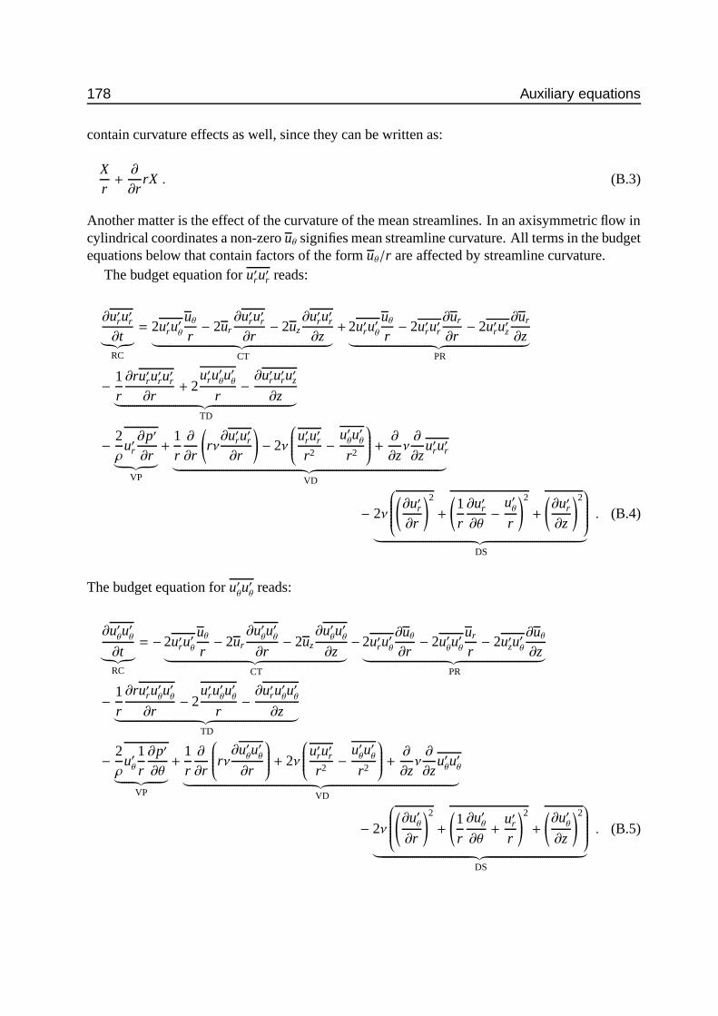
178 Auxiliary equations
contain curvature effects as well, since they can be written as:
Xr+∂
∂rrX . (B.3)
Another matter is the effect of the curvature of the mean streamlines. In an axisymmetric flow incylindrical coordinates a non-zero uθ signifies mean streamline curvature. All terms in the budgetequations below that contain factors of the form uθ/r are affected by streamline curvature.
The budget equation for u′ru′r reads:
∂u′ru′r∂t︸︷︷︸RC
= 2u′ru′θ
uθr− 2ur
∂u′ru′r∂r− 2uz
∂u′ru′r∂z︸ ︷︷ ︸
CT
+ 2u′ru′θ
uθr− 2u′ru′r
∂ur
∂r− 2u′ru′z
∂ur
∂z︸ ︷︷ ︸PR
− 1r
∂ru′ru′ru′r∂r
+ 2u′ru′θu′θ
r−∂u′ru′ru′z∂z︸ ︷︷ ︸
TD
− 2ρ
u′r∂p′
∂r︸ ︷︷ ︸VP
+1r∂
∂r
(rν∂u′ru′r∂r
)− 2ν
u′ru′rr2−
u′θu′θ
r2
+∂
∂zν∂
∂zu′ru′r
︸ ︷︷ ︸VD
− 2ν
(∂u′r∂r
)2
+
(1r
∂u′r∂θ−
u′θ
r
)2
+
(∂u′r∂z
)2
︸ ︷︷ ︸DS
. (B.4)
The budget equation for u′θu′θ
reads:
∂u′θu′θ
∂t︸︷︷︸RC
= − 2u′ru′θ
uθr− 2ur
∂u′θu′θ
∂r− 2uz
∂u′θu′θ
∂z︸ ︷︷ ︸CT
− 2u′ru′θ
∂uθ∂r− 2u′
θu′θ
ur
r− 2u′zu
′θ
∂uθ∂z︸ ︷︷ ︸
PR
− 1r
∂ru′ru′θu′θ
∂r− 2
u′ru′θu′θ
r−∂u′ru
′θu′θ
∂z︸ ︷︷ ︸TD
− 2ρ
u′θ
1r∂p′
∂θ︸ ︷︷ ︸VP
+1r∂
∂r
rν∂u′
θu′θ
∂r
+ 2ν
u′ru′rr2−
u′θu′θ
r2
+∂
∂zν∂
∂zu′θu′θ
︸ ︷︷ ︸VD
− 2ν
(∂u′
θ
∂r
)2
+
(1r
∂u′θ
∂θ+
u′rr
)2
+
(∂u′
θ
∂z
)2
︸ ︷︷ ︸DS
. (B.5)

B.1 Equations in cylindrical coordinates 179
The budget equation for u′zu′z reads:
∂u′zu′z∂t︸︷︷︸RC
= − ur∂u′zu′z∂r− uz
∂u′zu′z∂z︸ ︷︷ ︸
CT
− 2u′ru′z∂uz
∂r− 2u′zu′z
∂uz
∂z︸ ︷︷ ︸PR
− 1r
∂ru′ru′zu′z∂r
−∂u′ru′zu′z∂z︸ ︷︷ ︸
TD
− 2ρ
u′z∂p′
∂z︸ ︷︷ ︸VP
+1r∂
∂r
rν∂u′zu′z∂r
+∂
∂zν∂
∂zu′zu′z
︸ ︷︷ ︸VD
− 2ν
(∂u′z∂r
)2
+
(1r
∂u′z∂θ
)2
+
(∂u′z∂z
)2
︸ ︷︷ ︸DS
. (B.6)
The budget equation for u′ru′z reads:
∂u′ru′z∂t︸︷︷︸RC
= + u′zu′θ
uθr− ur
∂u′ru′z∂r− uz
∂u′ru′z∂z︸ ︷︷ ︸
CT
− u′ru′r∂uz
∂r+ u′zu
′θ
uθr− u′ru′z
∂uz
∂z− u′ru′z
∂ur
∂z− u′zu′z
∂ur
∂z︸ ︷︷ ︸PR
− 1r
∂ru′ru′ru′z∂r
+u′ru′θu′θ
r−∂u′ru′zu′z∂z︸ ︷︷ ︸
TD
− 1ρ
u′z∂p′
∂r− 1ρ
u′r∂p′
∂z︸ ︷︷ ︸VP
+1r∂
∂r
rν∂u′ru′z∂r
− νu′ru′zr2+∂
∂zν∂
∂zu′ru′z
︸ ︷︷ ︸VD
− 2ν
∂u′r∂r
∂u′z∂r+
(1r
∂u′r∂θ−
u′θ
r
)1r
∂u′z∂θ+∂u′r∂z
∂u′z∂z
︸ ︷︷ ︸
DS
. (B.7)
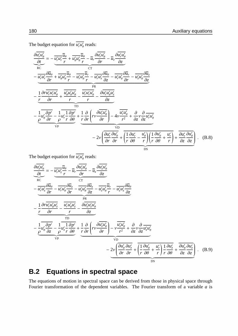
180 Auxiliary equations
The budget equation for u′ru′θ
reads:
∂u′ru′θ
∂t︸︷︷︸RC
= − u′ru′ruθr+ u′
θu′θ
uθr− ur
∂u′ru′θ
∂r− uz
∂u′ru′θ
∂z︸ ︷︷ ︸CT
− u′ru′r∂uθ∂r+ u′
θu′θ
uθr− u′ru
′θ
ur
r− u′ru′z
∂uθ∂z− u′ru
′θ
∂ur
∂r− u′zu
′θ
∂uz
∂z︸ ︷︷ ︸PR
− 1r
∂ru′ru′ru′θ
∂r+
u′θu′θu′θ
r−
u′ru′ru′θ
r−∂u′ru
′θu′z
∂z︸ ︷︷ ︸TD
− 1ρ
u′θ
∂p′
∂r− 1ρ
u′r1r∂p′
∂θ︸ ︷︷ ︸VP
+1r∂
∂r
rν∂u′ru
′θ
∂r
− 4νu′ru′θ
r2+∂
∂zν∂
∂zu′ru′θ
︸ ︷︷ ︸VD
− 2ν
∂u′r∂r
∂u′θ
∂r+
(1r
∂u′r∂θ−
u′θ
r
) (1r
∂u′θ
∂θ+
u′rr
)+∂u′r∂z
∂u′θ
∂z
︸ ︷︷ ︸
DS
. (B.8)
The budget equation for u′zu′θ
reads:
∂u′zu′θ
∂t︸︷︷︸RC
= − u′ru′zuθr− ur
∂u′zu′θ
∂r− uz
∂u′zu′θ
∂z︸ ︷︷ ︸CT
− u′ru′z∂uθ∂r− u′ru
′θ
∂uz
∂r− u′zu
′θ
∂uz
∂z− u′zu
′θ
ur
r− u′zu′z
∂uθ∂z︸ ︷︷ ︸
PR
− 1r
∂ru′ru′θu′z
∂r−
u′ru′θu′z
r−∂u′zu′zu
′θ
∂z︸ ︷︷ ︸TD
− 1ρ
u′θ
∂p′
∂z− 1ρ
u′z1r∂p′
∂θ︸ ︷︷ ︸VP
+1r∂
∂r
rν∂u′zu
′θ
∂r
− νu′zu′θ
r2+∂
∂zν∂
∂zu′zu′θ
︸ ︷︷ ︸VD
− 2ν
∂u′
θ
∂r
∂u′z∂r+
(1r
∂u′θ
∂θ+
u′rr
)1r
∂u′z∂θ+∂u′
θ
∂z
∂u′z∂z
︸ ︷︷ ︸
DS
. (B.9)
B.2 Equations in spectral spaceThe equations of motion in spectral space can be derived from those in physical space throughFourier transformation of the dependent variables. The Fourier transform of a variable a is

B.2 Equations in spectral space 181
denoted by a. Fourier transformed variables are a function of the wave vector kkk rather thanthe spatial coordinate x.
B.2.1 Navier-Stokes equations in spectral spaceThe Navier-Stokes equations in spectral space read (Lesieur, 1993):
(∂
∂t+ νkkk · kkk
)uuu = −i
(δδδ − kkkkkk
kkk · kkk
) [∫
ppp+qqq=kkkuuu(ppp)uuu(qqq)dppp
]· kkk , (B.10)
where i2= 1. The term δδδ − kkkkkk
kkk·kkk is a projector operator that projects onto a plane perpendicular tokkk.
B.2.2 Reynolds stress budget equationsFor a turbulent flow with a mean shear tensor λλλ, the budget equation for the spectral stress tensor
ΦΦΦ(= uuu′uuu′) is (see Bertoglio, 1982):
∂
∂tΦΦΦ − kkk · λλλ · ∇∇∇ΦΦΦΦΦΦΦΦΦ = −
(2(I − kkkkkk
kkk · kkk ) · λλλ ·ΦΦΦ + 2ΦΦΦ · λλλT · (I − kkkkkkkkk · kkk )
)− 2νkkk · kkkΦΦΦ + TTT , (B.11)
where TTT is a collection of all non-linear terms (including the so-called slow pressure-strain term).The first term at the right hand side includes the spectral representation of the rapid pressure-strain term. It can be shown that —since the flow is incompressible— this term does not changethe turbulent kinetic energy, though it does change the individual components. For isotropicturbulence we can show that pure rotation (i.e. an antisymmetric λλλ) does not influenceΦΦΦthroughthe linear terms.

182 Auxiliary equations
COn the relationshipbetween streamline
curvature and rotation inswirling flows
In discussions on turbulent swirling flows the effects of streamline curvature and rotation on theturbulence is a recurring topic. In these discussions streamline curvature and rotation seem to bedifferent issues. This distinction, however, partly stems from the origin of the interest in stream-line curvature versus rotation: aerodynamics versus geophysical flows. In the first type of flows anatural radius of curvature can be identified (curvature of the wing under consideration), whereasin the second category a natural rotation rate is present (viz. that of the earth). Another reasonfor the analysis of flows in terms of a rotating reference frame is the fact that the characteristicsof the reference frame (the rotation rate in particular) are constant in space and –if appropriate–in time. This makes the mathematical description of phenomena in such a flow simpler.
In this appendix the link between the streamline curvature and rotation will be shown for thespecial case of swirling flows1.
C.1 Two reference framesThe discussion will be restricted to incompressible flow of a Newtonian fluid, which can bedescribed with the Navier-Stokes equation:
∂uuu∂t+∇∇∇ · uuuuuu = −1
ρ∇∇∇p + ν∇∇∇ · SSS (C.1)
This description is valid in an inertial reference frame. In order to clarify the relationship betweenstreamline curvature and rotation, two new reference frames will be introduced:
a. A reference frame that translates with the local velocity ucucuc. The path traced through spaceby this reference frame follows a streakline and has a local radius of curvature of RcRcRc. Notethat although in this frame the velocity uuu is zero, the spatial derivatives need not be zero.
b. A reference frame that rotates at an angular velocityΩΩΩ. The position vector of the point ofinterest, relative to the axis of rotation is RrRrRr.
1Here rotation and streamline curvature will be considered as two sides of the same phenomena. However,situations are conceivable in which the streamline curvature and rotation are not related, e.g. the flow through arotating, curved channel (Matsson and Alfredsson, 1990)
183
184 On the relationship between streamline curvature and rotation in swirling flows
In terms of the first reference frame the Navier-Stokes equation becomes:
∂uuu∂t+∇∇∇ · uuuuuu = −1
ρ∇∇∇p + ν∇∇∇ · SSS − 2
(RcRcRc
|RcRcRc|× ucucuc
|RcRcRc|
)× uuu +
(∣∣∣∣∣RcRcRc
|RcRcRc|× ucucuc
|RcRcRc|
∣∣∣∣∣)2
RcRcRc
− 2
(RcRcRc
|RcRcRc|× ucucuc
|RcRcRc|
)× ucucuc , (C.2)
where the factor(
RcRcRc
|RcRcRc | ×ucucuc
|RcRcRc |
)can be interpreted as a local rotation rate of the coordinate system. It
appears that streamline curvature yields three additional terms:
• a Coriolis-like term• a centrifugal acceleration• a term that looks like a Coriolis term, but has one important difference: it relates to the
translation velocity vector ucucuc rather than the velocity in the moving reference frame.
The first term will be zero, since in the moving reference frame the velocity is zero. Upon closerinspection it appears that the last term is twice the last but one term, (in magnitude and direction).Taking these considerations into account, the following version of the Navier-Stokes equationsresults:
∂uuu∂t+ ∇∇∇ · uuuuuu = −1
ρ∇∇∇p + ν∇∇∇ · SSS + 3
(∣∣∣∣∣RcRcRc
|RcRcRc|× ucucuc
|RcRcRc|
∣∣∣∣∣)2
RcRcRc . (C.3)
Thus the effect of of the curved path is expressed purely as a centrifugal acceleration. For a flowwithout curvature, i.e. Rc →∞, the centrifugal acceleration disappears.
The second reference frame simply yields the Navier Stokes equations with added centrifugaland Coriolis accelerations:
∂uuu∂t+∇∇∇ · uuuuuu = −1
ρ∇∇∇p + ν∇∇∇ · SSS + Ω2RrRrRr − 2ΩΩΩ × uuu . (C.4)
For the flow in a system without rotation, i.e. ΩΩΩ = 0, the extra terms disappear.
C.2 Application to swirling flowsC.2.1 Solid-body rotation without an axial velocity componentOnly for a very simple flow a clear connection can be made between the Navier-Stokes equa-tions in both reference frames. This simple swirling flow2 is a two-dimensional rotating flow atconstant angular speed. In this flow both a natural radius of curvature and a natural rotation ratecan be identified. In terms of the first reference frame the magnitude of ucucuc and RcRcRc are constant aswell as the magnitude and direction of RcRcRc × ucucuc in terms of the first reference frame –for a givenpoint in the flow. In the second reference frame, justΩΩΩ is constant.
2According to the definition of a swirling flow in section 2.2 this is not a swirling flow

C.2 Application to swirling flows 185
The link between (C.2) and (C.4) for the simple flow under consideration is clear: the lattercan be derived from the first by replacing uuu by uuu − ucucuc and RcRcRc
|RcRcRc | ×ucucuc
|RcRcRc | by ΩΩΩ. Thus (C.4) is just aspecial form of (C.2). Note that for this special case the Coriolis term in (C.4) translates into acentrifugal term.
C.2.2 Solid-body rotation including an axial velocity componentIn a real swirling flow the radius of curvature is not only determined by the tangential velocity,but by the combined effect of tangential and axial velocity. Indeed, at infinite axial velocity theradius of curvature would also be infinite (no curvature) despite any non-zero tangential velocitycomponent. For the second reference frame again there is a natural rotation rate, viz. the angularvelocity corresponding to the solid-body rotation. But now no longer the Coriolis term acts as acentrifugal acceleration due to the fact thatΩΩΩ is no longer perpendicular to the velocity vector uuu.
C.2.3 General rotation including an axial velocity componentIn the case of a general swirling flow the description of the flow in terms of streamline curvature isstill useful. On the other hand, only in very special cases a natural rotation rate can be identifiedto use with the second reference frame. An example where it is possible is the flow througha rotating pipe (Imao et al., 1996; Murakami and Kikuyama, 1980; Orlandi and Fatica, 1997;Reich and Beer, 1989). Also parts of a flow in which the tangential velocity profile is that of asolid-body rotation could be analysed in terms of the second reference frame.
As in the previous section, for these more realistic swirling flows, the effect of the rotatingreference frame appears as both a centrifugal term and a Coriolis term.

186 On the relationship between streamline curvature and rotation in swirling flows

DErrors in LDA
measurements due togeometrical uncertainties
Section 3.2.2 described the way in which various positions and angles in the LDA system havebeen set to their appropriate values (mutual orientation of the laser beams and orientation of theLDA optics relative to the pipe). These alignments all have a finite accuracy. Steenbergen (1995)has analysed the effect of these inaccuracies on the measured mean velocities and turbulentstresses. For easier reference his results (not the derivations) are reproduced here (from section4.4 in his thesis).
D.1 Error due to imperfection of theodolite calibrationThe mutual angles of the three laser beams (two reference beams and the scattering beam) hasbeen determined with a theodolite. For the front lens with f = 160mm, for which the anglebetween beam and optical axis is 80, a typical error in the direction of the beams is 0.020. Theerrors in the mean velocities due to inaccuracies in this theodolite calibration are (for a definitionof the axes, see below (3.6) on page 47):
δu1 = ±0.003u1 ± 0.002u2 ± 0.0005u3
δu2 = ±0.003u1 ± 0.005u2 ± 0.0005u3 (D.1)
Errors in turbulent stresses are:
δu′1u′1 = ±0.006u′1u′1 ± 0.004u′1u′2 ± 0.001u′1u′3δu′2u′2 = ±0.006u′2u′2 ± 0.01u′1u′2 ± 0.001u′2u′3δu′1u′2 = ±0.008u′1u′2 ± 0.003u′1u′1 ± 0.002u′2u′2 ± 0.0005u′1u′3 ± 0.0005u′2u′3 (D.2)
D.2 Errors due to imperfections of the positioning ofthe LDA
If the LDA has been aligned with the pipe perfectly, the velocity components u1 and u2 coincidewith the axial velocity and the velocity perpendicular to the plane through the pipe axis and theoptical axis of the LDA. Imperfections in this alignment can be expressed in rotations around theaxes x1, x2 and x3 (ψi, i = 1, 2, 3).
187

188 Errors in LDA measurements due to geometrical uncertainties
D.2.1 Rotation around the x1-axisIf the positioning error consists of a rotation around the x1 axis, cross-talk will appear betweenvelocity components u2 and u3. If the rotation is assumed to be ±0.070 the errors in the meanflow will only comprise an error in u2:
δu2 = ±0.001u3 (D.3)
The errors in the Reynolds stresses are:
δu′2u′2 = ±0.002u′2u′3δu′1u′2 = ±0.001u′1u′3 (D.4)
D.2.2 Rotation around the x2-axisIf the optical axis of the LDA is not exactly perpendicular to the pipe axis, cross-talk betweenvelocity components u1 and u3 will result. Assuming an erroneous rotation of ±150, this impliesfor the mean flow this:
δu1 = 0.003u3 (D.5)
Errors in the Reynolds stresses will be:
δu′1u′1 = ±0.006u′1u′3δu′1u′2 = ±0.003u′2u′3 (D.6)
D.2.3 Rotation around the x3-axisAn erroneous rotation around the x3-axis (optical axis) will result in cross-talk between the ve-locity components u1 and u2. For this error a rotation angle of ±0.20 is assumed. This gives thefollowing errors in the mean velocity components:
δu1 = ±0.0035u2
δu2 = ∓0.0035u1 (D.7)
The effect on the Reynolds stresses will be:
δu′1u′1 = ±0.007u′1u′2δu′2u′2 = ±0.007u′1u′2δu′1u′2 = ±0.0035
(u′1u′1 − u′2u′2
)(D.8)
D.3 Errors in 3D measurementsIn order to derive information about all three velocity components (three mean velocities and sixindependent Reynolds stresses), measurements need to be performed at three angles ψ (rotations
D.4 Application of error estimates 189
around the pipe axis, see section 3.2.2 and equation (3.7b). Errors in the angles ψ will result incrosstalk between uθ and ur. An error in the angle ψ of 0.050 will be assumed. The errors in themean velocities depends the choice of the combination of angles ψ. For ψ equal to 00 and 450:
δuθ = ±0.001ur
δur = ±0.001uθ ± 0.002ur , (D.9)
and for −450 and 450):
δuθ = ±0.001uθ ± 0.001ur
δur = ±0.001uθ ± 0.001ur . (D.10)
The errors in the various Reynolds stresses will be:
δu′ru′r = ±0.002u′ru′θ± 0.002u′
θu′θ
δu′θu′θ= ±0.007u′ru
′θ
δu′zu′θ= ±0.001u′ru′z
δu′ru′z = ±0.001u′zu′θ± 0.002u′ru′z
δu′ru′θ= ±0.001
(u′ru′r − u′
θu′θ
)(D.11)
D.4 Application of error estimatesIn order to make an estimate of the total error in mean velocities and stresses due to alignmenterrors, the individual error estimates as given in sections D.1 to D.3 need to combined. This isdone as follows:
• The errors mentioned in D.1 and D.2 are applied to the measured values of means and(co-)variances of u1 and u2 for each of the three angles (00, −450 and +450).
• These errors are summed and translated to errors in the means and (co-)variances of uz, uθand ur through the same transformation as with which the means and (co-)variances arecomputed themselves (the inverse of (3.7b) and (3.8c)).
• The resulting error is added to the errors according to the equations presented in sectionD.3.

190 Errors in LDA measurements due to geometrical uncertainties
E Details on the LES model
In this appendix some detailed features of the LES model discussed in section 4.2 are shown.
E.1 Example of equations in transformed coordinatesTo illustrate the consequences of the coordinate transformation defined in (4.29) and (4.30), thecontinuity equation and z component of the momentum equations will be given in the trans-formed coordinate system. The continuity equation in the new coordinate becomes (compare to2.11):
1f (ζ)ρ
∂ρur
∂ρ+
1f (ζ)ρ
∂uθ∂φ+∂w∂ζ− ρ
f (ζ)∂ f (ζ)∂ζ
∂uz
∂ρ= 0 (E.1)
The z -component of the momentum equations becomes (compare to B.1)
∂uz
∂t+
1f (ζ)ρ
∂ρuruz
∂ρ+
1f (ζ)ρ
∂uθuz
∂φ+∂uzuz
∂ζ− ρ
f (ζ)∂ f (ζ)∂ζ
∂uzuz
∂ρ=
− ∂p∂ζ+
ρ
f (ζ)∂ f (ζ)∂ζ
∂p∂ρ+
1f (ζ)
1ρ
∂ρσrz
∂ρ+
1f (ζ)
1ρ
∂σθz
∂φ+∂σzz
∂ζ− ρ
f (ζ)∂ f (ζ)∂ζ
∂σzz
∂ρ(E.2)
where the first line is the time rate of change, the second line gives the advection terms, the thirdline the pressure gradient term and the last line represents the diffusive term. The representationof the different stresses (σrz, σθz and σzz) is left undefined. In the present implementation thesestresses will comprise both the viscous part and the subgrid-scale stress.
E.2 Example of spatial discretisation: divergenceHere one example is given to illustrate the procedure: the divergence.
The divergence is integrated over the grid volume surrounding a pressure point.
∫ ζk
ζk−1
∫ φ j
φ j−1
∫ ρui
ρui−1
[1
f (ζ)ρ∂ρu∂ρ+
1f (ζ)ρ
∂v∂φ+∂w∂ζ− R
f (ζ)∂ f (ζ)∂ζ
∂w∂ρ
]f 2(ζ)ρdρdφdζ (E.3)
191

192 Details on the LES model
Integration of the first term gives:
∫ ζk
ζk−1
∫ φ j
φ j−1
∫ ρui
ρui−1
[1
f (ζ)ρ∂ρur
∂ρ
]f 2(ζ)ρdρdφdζ
=
∫ ζk
ζk−1
f (ζ)∫ φ j
φ j−1
[ρur]
ρui
ρui−1
]dφdζ
≈ f pk dφdζ(ρu
i ui, j,kr − ρu
i−1u i−1, j,kr )
(E.4)
The second term:∫ ζk
ζk−1
∫ φ j
φ j−1
∫ ρui
ρui−1
[1
f (ζ)ρ∂uθ∂φ
]f 2(ζ)ρdρdφdζ
=
∫ ζk
ζk−1
f (ζ)∫ ρu
i
ρui−1
[uθ]
φ j
φ j−1
]dρdζ
≈ f pk dρidζ (u i, j,k
θ− u i, j−1,k
θ)
(E.5)
The third term:∫ ζk
ζk−1
∫ φ j
φ j−1
∫ ρui
ρui−1
[∂uz
∂ζ
]f 2(ζ)ρdρdφdζ
≈∫ φ j
φ j−1
∫ ρui
ρui−1
[f 2(ζ)uz]
ζk
ζk−1
]ρdρdφ
≈f wk
2u i, j,kz − f w
k−12u i, j,k−1
z
ρ
pi dρidφ
(E.6)
And finally the fourth term:
∫ ζk
ζk−1
∫ φ j
φ j−1
∫ ρui
ρui−1
[− ρ2
f (ζ)∂ f (ζ)∂ζ
∂uz
∂ρ
]f 2(ζ)dρdφdζ
= −∫ φ j
φ j−1
∫ ζk
ζk−1
f (ζ)∂ f (ζ)∂ζ
∫ ρui
ρui−1
[ρ2∂uz
∂ρ
]dρdζdφ
≈ −∫ φ j
φ j−1
∫ ζk
ζk−1
f (ζ)∂ f (ζ)∂ζ
[ρ2w]
ρuiρu
i−1
]dζdφ
≈ − f pk d f p
k
[ρu
i2 14
(u i+1, j,k−1
z + u i, j,k−1z + u i+1, j,k
z + u i, j,kz
)−
ρui−1
2 14
(u i, j,k−1
z + u i−1, j,k−1z + u i, j,k
z + u i−1, j,kz )
)]dζdφ
(E.7)
We have made a number of approximations in the derivation of the discrete divergence, inorder to obtain a divergence that –when integrated over the entire domain– will reduce to themass balance at the edges of the domain.

E.3 Details on boundary conditions 193
Then we have to divide the terms by the volume of the grid cell ( f pk
2ρ
pi dρidφdζ), so that the
discrete divergence becomes:
(ρui u i, j,k
r − ρui−1u i−1, j,k
r )
f pk ρ
pi dρi
+(u i, j,k
θ− u i, j−1,k
θ)
f pk dφρp
i
+f wk
2u i, j,kz − f w
k−12u i, j,k−1
z
f pk
2dζ
−d f p
k
f pk
ρu
i2 14
(u i+1, j,k−1
z + u i, j,k−1z + u i+1, j,k
z + u i, j,kz
)−
ρui−1
2 14
(u i, j,k−1
z + u i−1, j,k−1z + u i, j,k
z + u i−1, j,kz
)/(dρiρ
pi )
(E.8)
E.3 Details on boundary conditionsE.3.1 Implementation of wall boundary condition for ur
With the use of the discretized divergence equation it can be derived that:
u imax+1, j,kr =
ρpimax
ρpimax+1
u imax−1, j,kr +
d f pk
ρpimax+1
2
ρpimax+1
(u imax+1, j,k
z + u imax+1, j,k−1z
)−ρ
pimax
2
ρpimax+1
(u imax, j,k
z + u imax, j,k−1z
) (E.9)
E.3.2 Implementation of wall boundary condition for p′
The pressure gradient normal to the wall is determined from interpolated pressure values at radialpositions i = imax + 1 and i = imax and an axial position that lies on the wall normal that passesthrough the position of u imax, j,k
r at the wall (see figure E.1). The pressure values are obtained fromthe values at axial positions k − 1, k and k + 1) by quadratic interpolation 1:
p imax, j,kinterp =Aimax
k−1,k p imax, j,k−1+ Aimax
k,k p imax, j,k+ Aimax
k+1,k p imax, j,k
p imax+1, j,kinterp =Aimax+1
k−1,k p imax+1, j,k−1+ Aimax+1
k,k p imax+1, j,k+ Aimax+1
k+1,k p imax+1, j,k (E.10)
where Aimax and Aimax+1 are matrices2. Then, the requirement that ∂ p′ /∂n = 0 is equivalent to torequiring that p imax+1, j,k
interp = p imax, j,kinterp:
kmax∑
n=1
Aimax+1k,n p imax+1, j,n
=
kmax∑
n=1
Aimaxk,n p imax, j,n (E.11)
1It is assumed that ∂∂z f (ζ) = 0 (or α = 0 in figure E.1) for k = 1 and k = kmax, so that the coefficients for pi, j,0
and p i, j,kmax+1 are equal to zero. α = 0 at k = 1 and k = kmax implies that the pipe walls are parallel at the inflowand outflow planes. For the present type of calculations, this is not a very serious obstacle
2With reference to figure E.1, the elements of Aimaxi j are:
Aimaxk−1,k = (ximax+1 − 0)(ximax+1 − ltot)/(−ltot − 0)(−ltot − ltot),
Aimaxk,k = (ximax+1 + ltot)(ximax+1 − ltot)/(0 + ltot)(0 − ltot) and
Aimaxk+1,k = (ximax+1 + ltot)(ximax+1 − 0)/(ltot + ltot)(ltot − 0).
For Aimax+1i j similar expressions hold.

194 Details on the LES model
x
ximax+1tot
l
imax,j,k+1
imax,j,k
imax,j,k−1
imax+1,j,k+1
imax+1,j,k
α
imax
imax+1,j,k−1
Figure E.1: Determination of the pressure gradient normal to an inclined wall. The location of the in-terpolated pressure are denoted by large shaded dots, whereas the computational pressurenodes are shown as small black dots.
or:
p imax+1, j,k=
kmax∑
n=1
(AimaxAimax+1−1)
n,kp imax, j,n
=
kmax∑
n=1
Bn,k p imax, j,n. (E.12)
The approximations given above are valid as long as the slope of the wall does not change. Inthe present case study, however, the pipe walls are parallel at the inflow and outflow plane, anddo change slope in between. Therefore, some problems with respect to mass conservation maybe expected at the locations where the pipe wall has its maximum curvature (in axial direction).
E.4 Details on the radial grid spacingThe uniformity of the distribution of radial location of the grid points is controlled by a coefficientC. The radial location of the [[[r]-points (ρu
i ) is determined with the following recipe:
xi =i
imax,
yi = atanh(C)xi ,
zi = 0.5 tanh(yi) ,
ρui = zi + (0.5 − zimax)
iimax
. (E.13)
The last step ensures that the [[[r]-point for i = imax is located at the pipe wall. The factor i/imaxis introduced to prevent the points near the pipe axis to be moved away too far from the pipe axis.

E.5 Test of methods to generate swirl 195
The radial positions of the pressure points are taken halfway between the [[[r]-points:
ρpi =
12
(ρu
i + ρui−1
). (E.14)
E.5 Test of methods to generate swirlFor the LES model of the pipe contraction, the inflow boundary conditions for the velocities aregenerated with a separate LES model with periodic boundary conditions and parallel walls. Forthe simulations with swirl, the non-zero tangential velocity has to be introduced somehow. Twooptions have been presented in section 4.2.5: forcing through the tangential shear stress profile(equation (4.42), here method A) or through the mean tangential velocity (equation (4.40), heremethod B).
To test the quality of both methods low resolution simulations have been made with the LESmodel (see table E.1). It should be noted that the simulations for method A showed wiggles,even when the damping of those wiggles (see G.3) was increased. The results will be comparedwith the LDA data obtained at z/D = −1.8 in figures E.2 to E.9.
Figure E.2 shows the results for uz. The overall values of uz are correct due the normalisationused. The difference between the two forcing methods occurs near the pipe centre, where methodA gives a too pronounced jet. But even the uz-profile for method B gives too high values nearthe centre. Figure E.3 shows the resulting profiles for uθ. Here and important and anticipateddifference between the two methods appears: method A does not give the correct uθ-profile,whereas method B does. The results for the normal stresses are shown in figures E.4 to E.6. Ingeneral, the profiles of u′ru′r, u′
θu′θ
and u′zu′z are reproduced reasonably well, except near the centre.There the values are underpredicted by method A and overpredicted by method B. The axial shearstress u′ru′z is shown in figure E.7. Neither of the forcing methods is able to reproduce the negativevalue of u′ru′z near the pipe centre. The profile of u′ru′z hardly differs from that of a fully developedpipe flow without swirl: this reflects the fact that in the axial direction the flow is forced by apressure gradient that is independent of the radial position. The u′ru
′θ-profiles shown in figure E.8
give the anticipated result that method A gives a correct u′ru′θ-profile, since that profile was used
to determine the forcing. For forcing method B the u′ru′θ-profile is reproduced reasonably well in
the region r/R > 0.5, but near the pipe centre u′ru′θ
is overestimated strongly. Finally, the profilesof u′zu
′θ
are shown in figure E.9. For forcing method A the results are reasonably correct in theregion r/R < 0.5, whereas for method B the profile is correct for r/R > 0.5.
Based on these results method B will be used in the simulations presented in chapter 6.
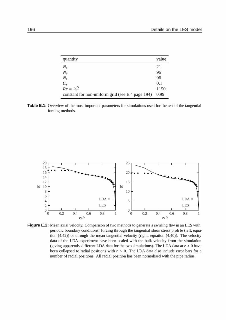
196 Details on the LES model
quantity value
Nr 21Nθ 96Nz 96Cs 0.1Re = u∗D
ν1150
constant for non-uniform grid (see E.4 page 194) 0.99
Table E.1: Overview of the most important parameters for simulations used for the test of the tangentialforcing methods.
LES
LDA
r/R
u z
10.80.60.40.20
201816141210
86420
LES
LDA
r/R
u z
10.80.60.40.20
25
20
15
10
5
0
Figure E.2: Mean axial velocity. Comparison of two methods to generate a swirling flow in an LES withperiodic boundary conditions: forcing through the tangential shear stress profile (left, equa-tion (4.42)) or through the mean tangential velocity (right, equation (4.40)). The velocitydata of the LDA-experiment have been scaled with the bulk velocity from the simulation(giving apparently different LDA data for the two simulations). The LDA data at r < 0 havebeen collapsed to radial positions with r > 0. The LDA data also include error bars for anumber of radial positions. All radial position has been normalised with the pipe radius.

E.5 Test of methods to generate swirl 197
LES
LDA
r/R
u θ
10.80.60.40.20
14
12
10
8
6
4
2
0LES
LDA
r/R
u θ
10.80.60.40.20
14
12
10
8
6
4
2
0
Figure E.3: Mean tangential velocity. Comparison of two methods to generate a swirling flow in an LESwith periodic boundary conditions: forcing through the tangential shear stress profile (left,equation (4.42)) or through the mean tangential velocity (right, equation (4.40)). For noteson normalisation, see E.2.
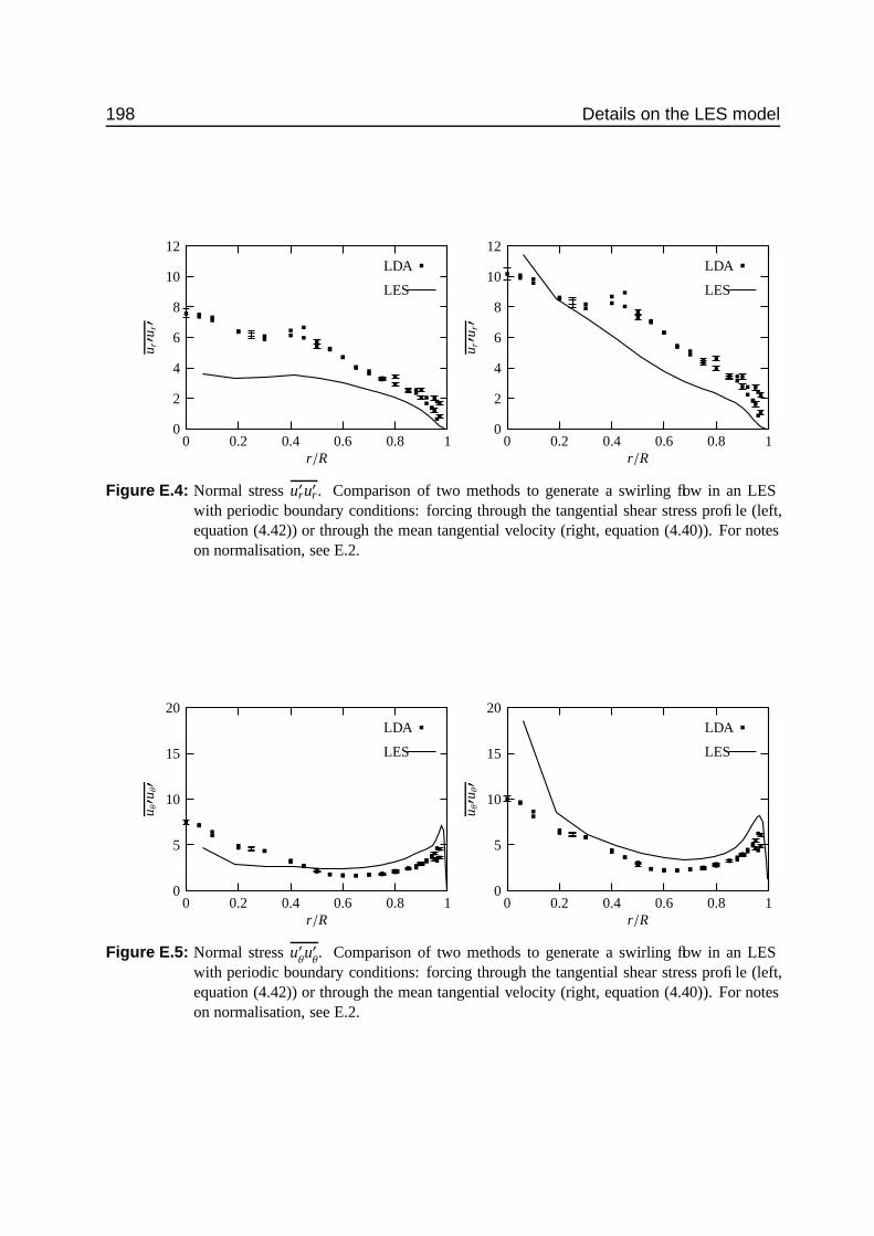
198 Details on the LES model
LES
LDA
r/R
u r′u
r′
10.80.60.40.20
12
10
8
6
4
2
0
LES
LDA
r/Ru r′u
r′
10.80.60.40.20
12
10
8
6
4
2
0
Figure E.4: Normal stress u′ru′r. Comparison of two methods to generate a swirling flow in an LESwith periodic boundary conditions: forcing through the tangential shear stress profile (left,equation (4.42)) or through the mean tangential velocity (right, equation (4.40)). For noteson normalisation, see E.2.
LES
LDA
r/R
u θ′u
θ′
10.80.60.40.20
20
15
10
5
0
LES
LDA
r/R
u θ′u
θ′
10.80.60.40.20
20
15
10
5
0
Figure E.5: Normal stress u′θu′θ. Comparison of two methods to generate a swirling flow in an LES
with periodic boundary conditions: forcing through the tangential shear stress profile (left,equation (4.42)) or through the mean tangential velocity (right, equation (4.40)). For noteson normalisation, see E.2.
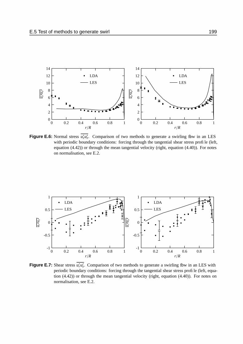
E.5 Test of methods to generate swirl 199
LES
LDA
r/R
u z′u
z′
10.80.60.40.20
14
12
10
8
6
4
2
0
LES
LDA
r/Ru z′u
z′
10.80.60.40.20
14
12
10
8
6
4
2
0
Figure E.6: Normal stress u′zu′z. Comparison of two methods to generate a swirling flow in an LESwith periodic boundary conditions: forcing through the tangential shear stress profile (left,equation (4.42)) or through the mean tangential velocity (right, equation (4.40)). For noteson normalisation, see E.2.
LES
LDA
r/R
u r′u
z′
10.80.60.40.20
1
0.5
0
-0.5
-1
LES
LDA
r/R
u r′u
z′
10.80.60.40.20
1
0.5
0
-0.5
-1
Figure E.7: Shear stress u′ru′z. Comparison of two methods to generate a swirling flow in an LES withperiodic boundary conditions: forcing through the tangential shear stress profile (left, equa-tion (4.42)) or through the mean tangential velocity (right, equation (4.40)). For notes onnormalisation, see E.2.

200 Details on the LES model
LES
LDA
r/R
u r′u
θ′
10.80.60.40.20
1.4
1.2
1
0.8
0.6
0.4
0.2
0LES
LDA
r/Ru r′u
θ′
10.80.60.40.20
1.4
1.2
1
0.8
0.6
0.4
0.2
0
Figure E.8: Shear stress u′ru′θ. Comparison of two methods to generate a swirling flow in an LES withperiodic boundary conditions: forcing through the tangential shear stress profile (left, equa-tion (4.42)) or through the mean tangential velocity (right, equation (4.40)). For notes onnormalisation, see E.2.
LES
LDA
r/R
u θ′u
z′
10.80.60.40.20
3
2
1
0
-1
-2
LES
LDA
r/R
u θ′u
z′
10.80.60.40.20
3
2
1
0
-1
-2
Figure E.9: Shear stress u′zu′θ. Comparison of two methods to generate a swirling flow in an LES withperiodic boundary conditions: forcing through the tangential shear stress profile (left, equa-tion (4.42)) or through the mean tangential velocity (right, equation (4.40)). For notes onnormalisation, see E.2.

FDependence of
simulations of developedpipe flow on size and
shape of the grid
In chapter 4 (sections 4.1.6 and 4.1.4) two issues have been raised with respect to the grid-dependence of simulation results: grid size dependence (section 4.1.6) and grid shape depen-dence (section 4.1.4).
F.1 Grid size dependence
The dependence of simulation results on the grid resolution has been tested with three grids.These are summarised in table F.1. The grid dependence of the bulk velocity is shown in figureF.1. For the two largest grids the simulated bulk velocity is well within 1% of the theoretical valueof 17.33 for the Reynolds number under consideration. The mean axial velocity, shown in figureF.2, also gives no clear difference between the two highest resolutions. The turbulent normalstresses (figures F.2 and F.3), on the other hand do show differences between all resolutions,where the results of the highest resolution come closest to the experimental data. For the u′ru′rand u′zu′z stress the simulation results nearly coincide with the laboratory data, whereas the u′
θu′θ
stress is still too low in the near-wall region. Finally the shear stress is shown in figure F.4.Given the fact that this stress should balance the pressure gradient forcing (which is identical forall simulations) the results do hardly differ between the different resolutions.
Configuration Result
name Nr Nθ Nz NL Ubulk
A 16 96 96 27.8 19.49B 33 156 156 51.0 17.42C 48 234 234 75.2 17.18
Table F.1: Characteristics of the three simulations. Nr, Nθ and Nz are the number of grid points in theradial, tangential and axial direction respectively.
201
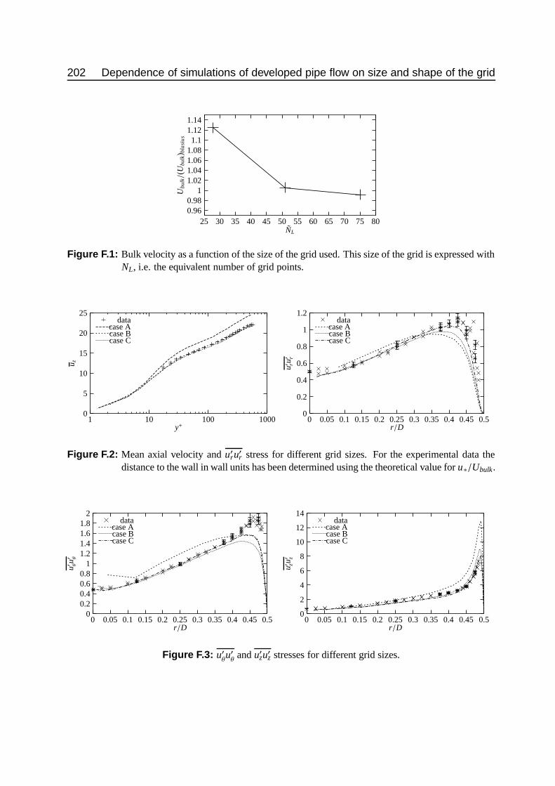
202 Dependence of simulations of developed pipe flow on size and shape of the grid
NL
Ubu
lk/(
Ubu
lk) b
lasi
us
807570656055504540353025
1.141.121.1
1.081.061.041.02
10.980.96
Figure F.1: Bulk velocity as a function of the size of the grid used. This size of the grid is expressed withNL, i.e. the equivalent number of grid points.
case Ccase Bcase A
data
y+
u z
1000100101
25
20
15
10
5
0
case Ccase Bcase A
data
r/D
u′ ru′ r
0.50.450.40.350.30.250.20.150.10.050
1.2
1
0.8
0.6
0.4
0.2
0
Figure F.2: Mean axial velocity and u′ru′r stress for different grid sizes. For the experimental data thedistance to the wall in wall units has been determined using the theoretical value for u∗/Ubulk.
case Ccase Bcase A
data
r/D
u′ θu′ θ
0.50.450.40.350.30.250.20.150.10.050
21.81.61.41.2
10.80.60.40.2
0
case Ccase Bcase A
data
r/D
u′ zu′ z
0.50.450.40.350.30.250.20.150.10.050
14
12
10
8
6
4
2
0
Figure F.3: u′θu′θ
and u′zu′z stresses for different grid sizes.

F.2 Grid shape dependence 203
case Ccase Bcase A
data
r/D
u′ ru′ z
0.50.450.40.350.30.250.20.150.10.050
1.2
1
0.8
0.6
0.4
0.2
0
Figure F.4: u′ru′z shear stress for different grid sizes.
Configuration Result
name Nr Nθ Nz Ubulk
A 21 128 128 18.35B 21 96 172 19.94C 21 172 96 18.02D 21 224 74 18.12
Table F.2: Characteristics of the four simulations. Nr, Nθ and Nz are the number of grid points in theradial, tangential and axial direction respectively.
F.2 Grid shape dependenceIn order to study the dependence of LES results on the aspect ratio of the grid cells, four simula-tions have been performed. All four simulations have the same number of grid points, but theydiffer in the allocation of those grid points to the different coordinate directions. The flow usedto study the dependence of LES results on the aspect ratio of the grid cells is a simple developedpipe flow through a straight pipe. The domain length is five pipe diameters and the turbulentReynolds number Re equals 1150. The characteristics of the four simulations are summarisedin table F.2. The theoretical value for the bulk velocity (from Blasius’ law) is 17.32. It is clearthat none of the simulations reaches this value. However, the simulations with a high resolutionin the tangential direction come closest to the theoretical value. This might support the claimthat in cylindrical coordinates a high tangential resolution is needed to faithfully represent theturbulence in the near-wall region (see section 4.1.4 and figure F.7)
In figures F.6 through F.8 the mean velocities and Reynolds stresses are compared betweenthe four simulations and with experimental data (see chapter 5). In figure F.5 the difference inbulk velocity between the different simulations is clearly visible. Although the differences in theReynolds stresses are not large, there is a clear tendency that the simulations with the highesttangential resolution (simulations C and D) are closest to the experimental data, especially in thenear-wall region.
The bump in the u′θu′θ
stress near the pipe axis seems to be worse for simulations with high

204 Dependence of simulations of developed pipe flow on size and shape of the grid
Nθ/Nz
Ubu
lk/(
Ubu
lk) b
lasi
us
3.532.521.510.5
1.21.181.161.141.121.1
1.081.061.041.02
1
Figure F.5: Bulk velocity as a function of the aspect ratio of the grid used. This aspect ratio is expressedas Nθ/Nz.
case Dcase Ccase Bcase A
data
y+
u z
1000100101
30
25
20
15
10
5
0
case Dcase Ccase Bcase A
data
r/D
u′ ru′ r
0.50.450.40.350.30.250.20.150.10.050
1.2
1
0.8
0.6
0.4
0.2
0
Figure F.6: Mean axial velocity and u′ru′r stress for different aspect ratios between axial and tangentialresolution. For the experimental data the distance to the wall in wall units has been deter-mined using the theoretical value for u∗/Ubulk.
tangential resolution. This strengthens the idea that the bump is due to the overresolution ofeddies near the pipe axis, where eddies are large, whereas the tangential grid spacing is verysmall.

F.2 Grid shape dependence 205
case Ccase Ccase Bcase A
data
r/D
u′ θu′ θ
0.50.450.40.350.30.250.20.150.10.050
21.81.61.41.2
10.80.60.40.2
0
case Dcase Ccase Bcase A
data
r/Du′ zu′ z
0.50.450.40.350.30.250.20.150.10.050
12
10
8
6
4
2
0
Figure F.7: u′θu′θ
and u′zu′z stresses for different aspect ratios between axial and tangential resolution.
case Dcase Ccase Bcase A
data
r/D
u′ ru′ z
0.50.450.40.350.30.250.20.150.10.050
1.2
1
0.8
0.6
0.4
0.2
0
Figure F.8: u′ru′z shear stress for different aspect ratios between axial and tangential resolution.

206 Dependence of simulations of developed pipe flow on size and shape of the grid
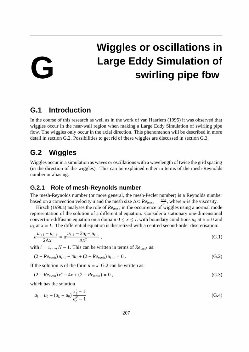
GWiggles or oscillations inLarge Eddy Simulation of
swirling pipe flow
G.1 IntroductionIn the course of this research as well as in the work of van Haarlem (1995) it was observed thatwiggles occur in the near-wall region when making a Large Eddy Simulation of swirling pipeflow. The wiggles only occur in the axial direction. This phenomenon will be described in moredetail in section G.2. Possibilities to get rid of these wiggles are discussed in section G.3.
G.2 WigglesWiggles occur in a simulation as waves or oscillations with a wavelength of twice the grid spacing(in the direction of the wiggles). This can be explained either in terms of the mesh-Reynoldsnumber or aliasing.
G.2.1 Role of mesh-Reynolds numberThe mesh-Reynolds number (or more general, the mesh-Peclet number) is a Reynolds numberbased on a convection velocity a and the mesh size ∆x: Remesh =
a∆xα
, where α is the viscosity.Hirsch (1990a) analyses the role of Remesh in the occurrence of wiggles using a normal mode
representation of the solution of a differential equation. Consider a stationary one-dimensionalconvection-diffusion equation on a domain 0 ≤ x ≤ L with boundary conditions u0 at x = 0 anduL at x = L. The differential equation is discretized with a centred second-order discretisation:
aui+1 − ui−1
2∆x= α
ui−1 − 2ui + ui−1
∆x2, (G.1)
with i = 1, ...,N − 1. This can be written in terms of Remesh as:
(2 − Remesh) ui−1 − 4ui + (2 − Remesh) ui+1 = 0 . (G.2)
If the solution is of the form u = κi G.2 can be written as:
(2 − Remesh) κ2 − 4κ + (2 − Remesh) = 0 , (G.3)
which has the solution
ui = u0 + (uL − u0)κi
2 − 1
κN2 − 1
(G.4)
207

208 Wiggles or oscillations in Large Eddy Simulation of swirling pipe flow
with
κ2 =2 + Remesh
2 − Remesh(G.5)
From the definition of κ2 one can see that when Remesh exceeds 2 an oscillatory solution willoccur. The amplitude of the oscillations is proportional to (uL − u0), i.e. depending on theboundary conditions.
When Remesh becomes large, the diffusion term in the original differential equation becomesnegligible. What remains is a singular perturbation of the original equation: the order of thedifferential equation is lowered and the new differential equation can not satisfy both boundaryconditions (Roache, 1976).
Given the analysis above, on could question why wiggles do not appear in LES of developedpipe flow (without swirl), whereas in those simulations Remesh will generally be much largerthan 2 (if ReD = 20000, ∆x = D/40, and the SGS viscosity is of the order of the molecularviscosity, Remesh = 250). The answer is most probably that wiggles do occur, but that theiramplitude, relative to the turbulent fluctuations is too small to observe them. As observed above,the amplitude of wiggles is proportional to uL − u0. When the boundary conditions are takenat the inflow and outflow plane of the pipe section, uL − u0 will be nearly zero if the flow ishomogeneous in the axial direction (or exactly zero in case of periodic boundary conditions).The largest difference uL − u0 can be found when focussing on one turbulent structure and willbe of the order of u∗.
The analysis in terms of Remesh does not provide a reason why wiggles are prominent inswirling flow simulations and not discernible in simulations of non-swirling flow.
G.2.2 AliasingIf the flow under consideration is nearly inviscid, the non-linear advection term u ∂u
∂x can generatefluctuations with wave numbers as high as twice the wavenumber that can be represented on thegrid. This high-wavenumber energy will be aliased to wavenumbers that can be represented onthe mesh (Hirsch, 1990b) and may occur as fluctuations with wavelength 2∆x or more.
Hirsch (1990a) gives an example of a centrally discretized gradient of u:(u∂u∂x
)
i
≈ ui
(ui+1 − ui−1
2∆x
). (G.6)
u can be represented in terms of a Fourier expansion
ui =
∑
k
v(k)e jki∆x , (G.7)
with j =√−1 and k is the wave number. Then the advection term becomes:
(u∂u∂x
)
i
≈∑
k1
∑
k2
v(k2)e jk2i∆x
v(k1)e jk1i∆x 12∆x
(e jk1∆x − e− jk1∆x
)(G.8)
≈ j∆x
∑
k1
∑
k2
v(k1)v(k2)e j(k1+k2))∆x sin k1∆x (G.9)
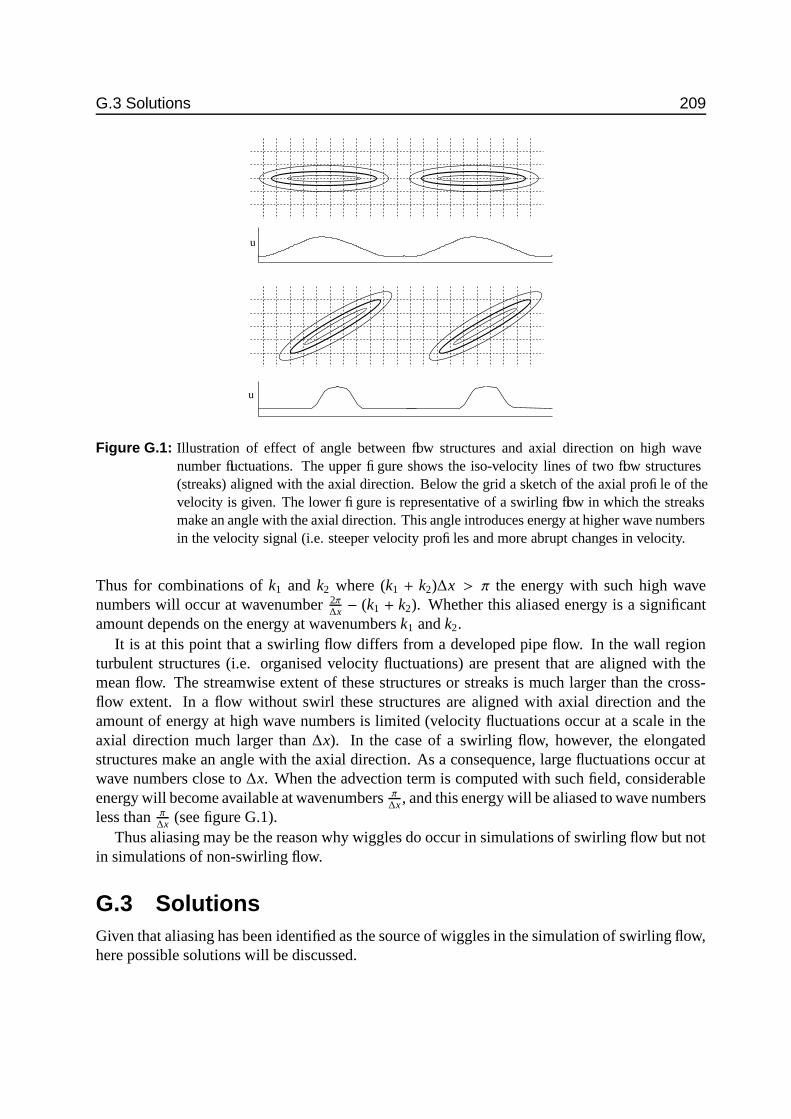
G.3 Solutions 209
u
u
Figure G.1: Illustration of effect of angle between flow structures and axial direction on high wavenumber fluctuations. The upper figure shows the iso-velocity lines of two flow structures(streaks) aligned with the axial direction. Below the grid a sketch of the axial profile of thevelocity is given. The lower figure is representative of a swirling flow in which the streaksmake an angle with the axial direction. This angle introduces energy at higher wave numbersin the velocity signal (i.e. steeper velocity profiles and more abrupt changes in velocity.
Thus for combinations of k1 and k2 where (k1 + k2)∆x > π the energy with such high wavenumbers will occur at wavenumber 2π
∆x − (k1 + k2). Whether this aliased energy is a significantamount depends on the energy at wavenumbers k1 and k2.
It is at this point that a swirling flow differs from a developed pipe flow. In the wall regionturbulent structures (i.e. organised velocity fluctuations) are present that are aligned with themean flow. The streamwise extent of these structures or streaks is much larger than the cross-flow extent. In a flow without swirl these structures are aligned with axial direction and theamount of energy at high wave numbers is limited (velocity fluctuations occur at a scale in theaxial direction much larger than ∆x). In the case of a swirling flow, however, the elongatedstructures make an angle with the axial direction. As a consequence, large fluctuations occur atwave numbers close to ∆x. When the advection term is computed with such field, considerableenergy will become available at wavenumbers π
∆x , and this energy will be aliased to wave numbersless than π
∆x (see figure G.1).Thus aliasing may be the reason why wiggles do occur in simulations of swirling flow but not
in simulations of non-swirling flow.
G.3 SolutionsGiven that aliasing has been identified as the source of wiggles in the simulation of swirling flow,here possible solutions will be discussed.

210 Wiggles or oscillations in Large Eddy Simulation of swirling pipe flow
The most fundamental way to remove aliasing is to find a way to resolve the energy that occursat wave numbers above π
∆x due to the advection term. Once that energy has been representedcorrectly it could be removed (filtered) from the simulation and the original resolution shouldbe sufficient to represent the resulting velocity field. In spectral space this should be ratherstraightforward, but in physical space the solution is less obvious.
In the case of LES a similar approach is possible. If in an LES the size of the filter with whichthe equations have been filtered is sufficiently larger than the grid size the fluctuations with wavenumbers above the wave number of the filter can still be represented. What should be done thenis to remove those high wave number fluctuations in order to prevent them from destroying thesimulation. In the case that the Smagorinsky model is used the filter size can be increased byincreasing Cs.
One could be tempted to increase the resolution since in that case waves with higher wavenumbers can be represented. But if the filterlength in an LES model is tied to the grid size adecrease in ∆z at the same time implies a decrease of the filter length 2∆∗ (see 4.15b), althoughit depends on the formulation of the effective grid spacing ∆∗ what the effect of a decrease in ∆zon ∆∗ is 1.
The most commonly used method to eliminate wiggles that are due to aliasing is to make thesimulation less inviscid, i.e. to increase the viscosity:
• One could choose a discretisation that has a leading discretisation error of odd order. Thiserror will introduce an artificial viscosity. The first-order upwind discretisation is an exam-ple of this. Tests with this discretisation have shown that indeed the wiggles disappear butat the cost of a very large artificial viscosity.
• One could decrease the Reynolds number of the flow to be simulated. This will result in asimulation of a flow that differs from the original problem.
• In the case of LES with the Smagorinsky model for SGS stresses, an increase of the filterlength through an increase of Cs indeed decreases the effective Reynolds number as well(where the effective Reynolds number is a Reynolds number based on the sum of molecularand SGS viscosity).
• One could filter the velocity fields at each time step to suppress the wiggles.
In the present simulations extra diffusion is applied based on an indicator for the occurrenceof wiggles. This will be discussed below.
In simulations of swirling flows with the present model it was observed that the wiggles onlyoccur in the axial direction. Furthermore, they were most obvious in ur. In order to removeor suppress wiggles one needs an indicator for the presence of wiggles. Here the second ordertransverse structure function of ur will be used, for two separations, viz. r = ∆z and r = 2∆z:
Fur ,z(r) = [ur(z + r) − ur(z)]2 (G.10)
1The formulation used in the present model, equation 4.37 has the special property that when ∆z becomes verysmall, ∆∗ no longer decrease. Consequently the filterlength does not decrease monotonously with ∆z. For thisparticular choice of ∆∗, an increase in the axial resolution may actually help to reduce aliasing.
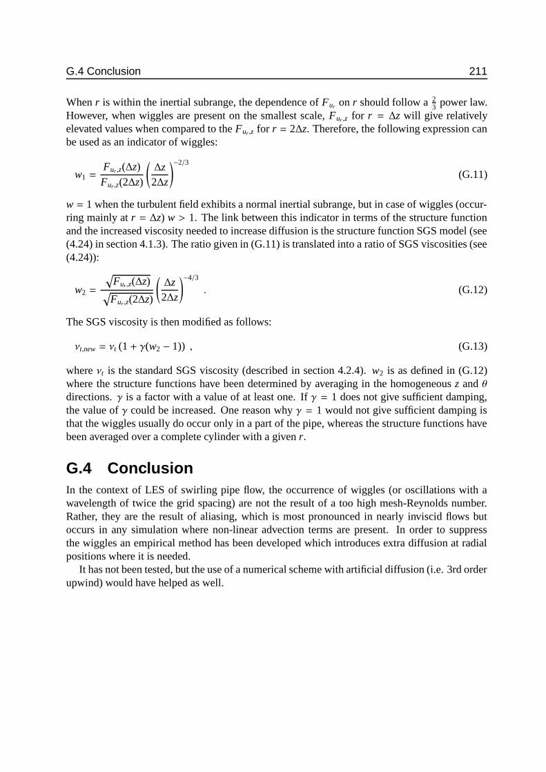
G.4 Conclusion 211
When r is within the inertial subrange, the dependence of Fur on r should follow a 23 power law.
However, when wiggles are present on the smallest scale, Fur ,z for r = ∆z will give relativelyelevated values when compared to the Fur ,z for r = 2∆z. Therefore, the following expression canbe used as an indicator of wiggles:
w1 =Fur ,z(∆z)
Fur,z(2∆z)
(∆z
2∆z
)−2/3
(G.11)
w = 1 when the turbulent field exhibits a normal inertial subrange, but in case of wiggles (occur-ring mainly at r = ∆z) w > 1. The link between this indicator in terms of the structure functionand the increased viscosity needed to increase diffusion is the structure function SGS model (see(4.24) in section 4.1.3). The ratio given in (G.11) is translated into a ratio of SGS viscosities (see(4.24)):
w2 =
√Fur ,z(∆z)
√Fur ,z(2∆z)
(∆z
2∆z
)−4/3
. (G.12)
The SGS viscosity is then modified as follows:
νt,new = νt (1 + γ(w2 − 1)) , (G.13)
where νt is the standard SGS viscosity (described in section 4.2.4). w2 is as defined in (G.12)where the structure functions have been determined by averaging in the homogeneous z and θdirections. γ is a factor with a value of at least one. If γ = 1 does not give sufficient damping,the value of γ could be increased. One reason why γ = 1 would not give sufficient damping isthat the wiggles usually do occur only in a part of the pipe, whereas the structure functions havebeen averaged over a complete cylinder with a given r.
G.4 ConclusionIn the context of LES of swirling pipe flow, the occurrence of wiggles (or oscillations with awavelength of twice the grid spacing) are not the result of a too high mesh-Reynolds number.Rather, they are the result of aliasing, which is most pronounced in nearly inviscid flows butoccurs in any simulation where non-linear advection terms are present. In order to suppressthe wiggles an empirical method has been developed which introduces extra diffusion at radialpositions where it is needed.
It has not been tested, but the use of a numerical scheme with artificial diffusion (i.e. 3rd orderupwind) would have helped as well.

212 Wiggles or oscillations in Large Eddy Simulation of swirling pipe flow

HPressure strain terms in
turbulent flow through anaxially rotating pipe: test
of models with DNS results
H.1 IntroOne of the terms in the budget equations for the Reynolds stresses is a covariance term that isthe covariance of a velocity component and the a pressure gradient (see appendix B). In the caseof an incompressible flow this term can be rewritten as the sum of a a pressure-strain term anda pressure diffusion term. In the practice of second order the latter is then combined with themodelling of the turbulence diffusion term. The pressure-strain tensor is (here written in indexnotation for Cartesian coordinates, for convenience)
Πi j =1ρ
p′S ′i j (H.1)
On one hand this term can not be measured in any physical experiment. On the other hand, it isthe dominant term in the budgets of those Reynolds stresses that have no direct production.
During the research for the current thesis, a side step has been made to analyse the data froma Direct Numerical Simulation (DNS) by Eggels et al. (1995) (a DNS of the turbulent flowthrough an axially rotating pipe). Since this flow bears some resemblance to the swirling flowstudied in the current research, the results will be presented here. The DNS results will be usedhere to determine the the pressure strain term as well as its rapid and slow part (section H.4.1).Furthermore, various models for the pressure strain tensor (section H.2) will be tested (sectionH.4.2). It should be kept in mind that this is an off-line test. It does not give direct informationon the skill of complete second-order closure models to model the flow under consideration.
H.2 Models for the pressure strain tensorThe modelling of Πi j generally involves the decomposition of the pressure fluctuations in a rapidand a slow part. This decomposition is based on the Poisson equation for p′:
1ρ∇2 p′ = −2
∂ui
∂x j
∂u′j∂xi− ∂2
∂xi∂x j
(u′iu′j − u′iu
′j
), (H.2)
where the first term on the RHS is the RHS for the Poisson equation of p′slow and the second isthe RHS of the Poisson equation of p′rapid. The problem in devising closures for Πi j is that p′ is
213

214 Pressure strain terms in turbulent flow through an axially rotating pipe
not a locally determined quantity, as the Poisson equation shows. Therefore, local closures areincorrect in principle, though they may be useful in practice.
If the turbulent quantities are locally homogeneous and all derivatives higher than first orderare zero for the mean flow, the Poisson equation can be solved to yield the following expressionfor Πi j:
Πi j = Ai j + Mi jkl∂uk
∂xl,
= ψi j,1 + ψi j,2 (H.3)
where the first term is the slow term and the second term is the rapid term. The tensors Ai j andMi jkl involve integrals of velocity fluctuations gradients over the entire domain. When a solidboundary is present in the domain, an extra term occurs in (H.3): a wall-reflection term. Below,a more or less random choice of models for the pressure-strain term will be summarised.
Rotta (1951) devised the following model for Ai j:
ψi j,1 = −C1ε
k
(u′iu′j −
23
kδi j
), (H.4)
where ε is the dissipation (= 12εkk), k is the turbulent kinetic energy (= 1
2u′iu′j) and δi j is the
Kronecker delta. For C1 a value of 1.8 will be used. For the normal stresses, Ai j is proportionalto the deviation of a normal stress to its isotropic value. This mechanism has led to the namereturn-to-isotropy term. For the shear stresses, the Rotta hypothesis leads to a return to a zeroshear stress, as Ai j is proportional to the deviation of the shear stress from zero. Two types ofextensions have been made to this model: the constant C1 has been made a function of the flow(more specifically: the stress invariants; see Launder (1989)) and an additional term has beenadded (see the model of Speziale et al. (1991), discussed below).
For the rapid term a number of closures have been devised (for an overview, see Wilcox(1993)). The ”Quasi-isotropic” model (QI-model, due to Launder et al. (1975)) is formulated as:
ψi j,2 = −α(Pi j −
13
Pkkδi j
)− β
(Di j −
13
Dkkδi j
)− γkS i j , (H.5)
with
Pi j = u′iu′m
∂u j
∂xm+ u′ju
′m
∂ui
∂xm
Di j = u′iu′m
∂um
∂x j+ u′ju
′m
∂um
∂xi
α =8 + C2
11, β =
8C2 − 211
, γ =60C2 − 4
55, 0.4 < C2 < 0.6 (H.6)
A modified version of the the ”Isotropisation of Production” model (IP-model) of Naot et al.(1970) due to Fu et al. (1987) is:
ψi j,2 = −C2
(Pi j −
13
Pkkδi j
)− C2
(Ci j −
13
Ckkδi j
), (H.7)

H.2 Models for the pressure strain tensor 215
with Pi j as above and
Ci j = ul
∂u′iu′j
∂xl. (H.8)
For the wall-reflection term, various models have been proposed. Here, the wall correction ofGibson and Launder (1978) is used as a correction relative to the QI-model (contrary to what isdone in the original paper where the formulation of the rapid part only includes the first term ofthe QI-model). The wall corrections for the slow and rapid part are:
ψi j,1w = C′1ε
k
(u′ku
′mnknmδi j −
32
u′ku′inkn j −
32
u′ku′jnkni
)k3/2
2.5εy(H.9)
ψi j,2w = C′2
(Gkmnknmδi j −
32
Giknkn j −32
G jknkni
)k3/2
2.5εy(H.10)
with: ni is the i-component of the normal to the wall, C′1 = 0.5, C′2 = 0.3, Gi j = −C2
(Pi j − δi jPkk
).
Note that in the original paper of Gibson and Launder (1978) the length scale correction is k3/2
κεy
with κ the Von Karman constant, rather than k3/2
2.5εy The second wall correction tested is the onedue to Craft and Launder (1992). The correction for the slow term is identical to the one useabove. The correction for the rapid term is:
ψi j,2w = − C2a∂ul
∂xmu′lu′m
(δi j − 3nin j
) k32
2.5εy
− C2bkalm
(∂uk
∂xmnlnkδi j −
32∂ui
∂xmnln j −
32
∂u j
∂xmnlni
)k3/2
2.5εy
+ C2ck∂ul
∂xmnlnm
(nin j −
13δi j
)k3/2
2.5εy(H.11)
with ai j = (u′iu′j − 2
3δi jk)/k, C′2a = 0.08, C′2b = 0.1 and C′2c = 0.4.Finally the model of Speziale et al. (1991) will be tested. This model (SSG-model) gives an
expression for the total pressure strain term (for a flow without system rotation):
Πi j = −(C′′1 ε + C′1∗Pkk
)ai j + C′′2 ε
(ai jak j −
13
amnanmδi j
)
+
(C′′3 − C′′3∗
√II
)kS i j + C′′4 k
(aikS jk + a jkS ik −
23
amnS mnδi j
)+ C′′5 k
(aikW jk + b jkWik
),
(H.12)
with S i j is the strain tensor, Wi j is the vorticity tensor 12
(∂ui
∂x j− ∂u j
∂xi
), C′′1 = 3.4, C′′1∗ = 1.8, C′′2 = 4.2,
C′′3 = 0.8, C′′3∗ = 1.3, C′′4 = 1.25, C′′5 = 0.4.. Pourahmadi and Humphrey (1985) show that theQI-model and the IP-model are just special cases of the SSG model (albeit with different valuesfor the coefficients).

216 Pressure strain terms in turbulent flow through an axially rotating pipe
H.3 The flow and the simulationIn order to test the relative importance of the rapid and slow part of the pressure strain correlation,as well as the quality of the different parameterisations, use will be made of velocity and pressurefields of the DNS ’C’ experiment of Eggels et al. (1995). This DNS experiment concerns arotating pipe with a domain length of 5 diameters D. The bulk Reynolds number Reb is 5860, theturbulent Reynolds number Re equals 360. The tangential velocity of the wall, uθ,w is 0.61Ubulk.The number of grid points in radial, tangential and axial direction is 96, 128, 256, respectively.Forty fields of ui and p are used in the analysis, all taken from the quasi-steady period after 10t∗
(t∗ = D/u∗), spanning a period of about 5t∗.
H.4 ResultsH.4.1 Simulation resultsBefore discussing the results presented here, two remarks based on the work of Eggels et al.(1995) need to be made:
• In most budgets the pressure strain term is the largest term;• All stresses are positive in this flow. Thus a positive sign of a budget term always signifies
a gain term and vice verse.
Figures H.1 to H.3 show the pressure strain terms for the normal stresses u′ru′r, u′θu′θ
and u′zu′z,respectively. Πrr is a gain term in the budget, except near the wall. The slow part and the rapidpart counteract, the slow term being the major gain term. For Πθθ the situation is quite different:except near the wall, the slow term is neglectable and the rapid part is the major gain term. ForΠzz the following can be noted: as could be expected –since the pressure-strain terms allow a fora return to isotropy– the pressure-strain term is a loss term for u′zu′z. The rapid and slow part playa role of about equal magnitude.
Figures H.4 to H.6 show the results for the shear stresses u′ru′θ, u′ru′z and u′zu
′θ, respectively. In
figure H.4 it can be seen that for u′ru′θ
the pressure strain correlation is a loss term, except nearthe wall. The slow part is practically zero throughout most of the crosssection, but acts as again term near the wall (contrary to the assumption of a return-to-isotropy). Πrz is neglectable orslightly positive in the central part of the pipe (up to r/D = 0.2. Except near the wall, the slowpart is a loss term, whereas the rapid part is negative throughout. The u′ru′z stress is the only shearstress that is being fed through the pressure-strain interactions also outside the wall region. Therapid part gives by far the largest contribution. The slow part is neglectable, except near the wall,where it is positive and this conflicting the idea of a return to isotropy.
H.4.2 Results on the parameterisationsThe results for the parameterisations of Πrr are shown in figures H.1. The models for the rapidpart differ in their ability to predict the negative rapid part near the wall. Only the models thatinclude a wall-correction do show that negative value. The models for the slow part of Πrr doshow the correct tendency, but give too high values and do not show the negative value near the

H.5 Conclusion 217
wall. The wall-correction does not help much in this case. The results for the total pressure-strainterm are that all models overestimateΠrr, except for the SSG model that predicts a Πrr that is toonegative. In figure H.2 it can be seen that the results for Πθθ are less diverse. Both for the rapidand the slow part all models give the correct tendency, although again the values are too high.Contrary to what occurred in the results of Πrr, the models including wall-correction give highervalues. The SSG model severely underestimates Πθθ. The results for Πzz (figure H.3) are verycomparable to those ofΠθθ, except for the fact that |Πrr is mostly positive andΠθθ is positive. Thistrend is correctly predicted by the models, but again with too large values. The large deviationof the results of the SSG model from those of the other models appears to be mainly due to theterm involving C′′1∗. The peaks in the pressure strain term coincide with the location of the peakin the production of the turbulent kinetic energy (Pkk). When C′′1∗ is set to zero more reasonablevalues result.
The results for Πrθ are given in figure H.4. For the slow part the various models give valuesthat are neglectable relative to the slow part derived from the DNS results. For the rapid part themodels diverge. The models show the correct tendency for r/D < 0.4 but for the region near thewall the results are incorrect. the local maximum at r/D ≈ 0.48 is only present in the results ofthe model of Craft and Launder (1992). For the total Πrθ all models show the correct tendency,withmost models giving too high (negative) values. Figure H.5 shows the results forΠrz. Both forthe rapid part, slow part and the total pressure-strain term the models with wall-correction showthe correct tendency. The SSG is completely off again. The first thing that is apparent in figureH.6 for Πθz is that there is no difference between the models with and without wall-correction.The models for the rapid part show the correct r-dependence, but the values are too low. Themodel results for the slow part are completely wrong. The results for the total Πθz are incorrect,with the SSG model being closest to the DNS results.
H.5 ConclusionFrom the analysis presented above it can be concluded that in the case of turbulent flow througha rotating pipe the rapid part of the pressure-strain terms is at least as important as the slow part.For some stresses, u′
θu′θ, u′ru
′θ
and u′zu′θ, the rapid part is the only important contributor to the
pressure-strain term. All models for the pressure-strain terms tested in this appendix are unableto represent the pressure-strain term correctly, except for a region close to the pipe centre. Forsome stresses the models do show the correct tendency. For the normal stresses the values aregenerally too large, for the shear stresses the values are of the correct order of magnitude.
It can be concluded that the present flow is still an interesting benchmark flow for Reynolds-stress models.

218 Pressure strain terms in turbulent flow through an axially rotating pipe
SSGCraft & LaunderGibson & LaunderIP-modelQI-modelDNS
r/D
Πrr
0.50.40.30.20.10
80
60
40
20
0
-20r/D
Πrr
0.50.40.30.20.10
80
60
40
20
0
-20r/D
Πrr
0.50.40.30.20.10
80
60
40
20
0
-20
Figure H.1: Pressure strain term for u′ru′r stress: total term (left), slow part (centre) and rapid part (right).Comparison between DNS results and four models for the respective terms.
SSGCraft & LaunderGibson & LaunderIP-modelQI-modelDNS
r/D
Πθθ
0.50.40.30.20.10
100
80
60
40
20
0
-20r/D
Πθθ
0.50.40.30.20.10
100
80
60
40
20
0
-20r/D
Πθθ
0.50.40.30.20.10
100
80
60
40
20
0
-20
Figure H.2: Pressure strain term for u′θu′θ
stress: total term (left), slow part (centre) and rapid part (right).Comparison between DNS results and four models for the respective terms.
SSGCraft & LaunderGibson & LaunderIP-modelQI-modelDNS
r/D
Πzz
0.50.40.30.20.10
20
0
-20
-40
-60
-80
-100r/D
Πzz
0.50.40.30.20.10
20
0
-20
-40
-60
-80
-100r/D
Πzz
0.50.40.30.20.10
20
0
-20
-40
-60
-80
-100
Figure H.3: Pressure strain term for u′zu′z stress: total term (left), slow part (centre) and rapid part (right).Comparison between DNS results and four models for the respective terms.
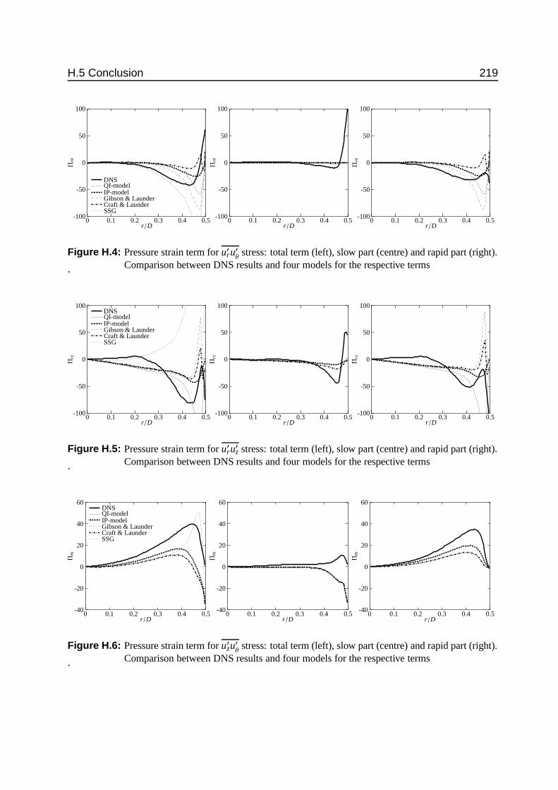
H.5 Conclusion 219
SSGCraft & LaunderGibson & LaunderIP-modelQI-modelDNS
r/D
Πrθ
0.50.40.30.20.10
100
50
0
-50
-100r/D
Πrθ
0.50.40.30.20.10
100
50
0
-50
-100r/D
Πrθ
0.50.40.30.20.10
100
50
0
-50
-100
Figure H.4: Pressure strain term for u′ru′θ stress: total term (left), slow part (centre) and rapid part (right).Comparison between DNS results and four models for the respective terms.
SSGCraft & LaunderGibson & LaunderIP-modelQI-modelDNS
r/D
Πrz
0.50.40.30.20.10
100
50
0
-50
-100r/D
Πrz
0.50.40.30.20.10
100
50
0
-50
-100r/D
Πrz
0.50.40.30.20.10
100
50
0
-50
-100
Figure H.5: Pressure strain term for u′ru′z stress: total term (left), slow part (centre) and rapid part (right).Comparison between DNS results and four models for the respective terms.
SSGCraft & LaunderGibson & LaunderIP-modelQI-modelDNS
r/D
Πθz
0.50.40.30.20.10
60
40
20
0
-20
-40r/D
Πθz
0.50.40.30.20.10
60
40
20
0
-20
-40r/D
Πθz
0.50.40.30.20.10
60
40
20
0
-20
-40
Figure H.6: Pressure strain term for u′zu′θ stress: total term (left), slow part (centre) and rapid part (right).Comparison between DNS results and four models for the respective terms.

220 Pressure strain terms in turbulent flow through an axially rotating pipe
Bibliography
Adrian R. (1996). Laser velocimetry. In: Fluid Mechanics Measurements (editor R. Goldstein),pp. 175–299. Taylor & Francis, Washington etc.
Aldama A.A. (1990). Filtering Techniques for Turbulent Flow Simulation, volume 56 of LectureNotes in Engineering. Springer Verlag, Berlin etc.
Aris R. (1989). Vectors, Tensors, and the Basic Equations of Fluid Mechanics. Dover, MineolaNY. (first published in 1962).
Arnal M. and Friedrich R. (1993). Large-eddy simulation of a turbulent flow with seperation. In:Durst et al. (1993), pp. 169–187.
Barbin A.R. and Jones J.B. (1963). Turbulent flow in the inlet region of a smooth pipe. J.BasicEngg., 85, 29–34.
Bardina J., Ferziger J.H. and Reynolds W.C. (1981). Improved subgrid models for large eddysimulation. AIAA Paper 80-1357.
Bardina J., Ferziger J.H. and Rogallo R.S. (1985). Effect of rotation on isotropic turbulence:computation and modelling. J. Fluid Mech., 154, 321–336.
Batchelor G.K. (1967). An Introduction to Fluid Dynamics. Cambridge University Press.Batchelor G.K. and Proudman I. (1954). The effect of rapid distortion of a fluid in turbulent
motion. Quart. J. Mech. Appl. Math., 7, 83–103.Bendat J.S. and Piersol A.G. (1986). Random Data: Analysis and Measurement Procedures.
John Wiley & Sons, 2nd edition.Benedict L.H. and Gould R.D. (1996). Uncertainty estimates for any turbulence statisic. In:
Proceedings of the 8th International Symposium on Applications of Laser Techniques to FluidMechanics, July 8-11. Paper 36.1.
van den Berg B. (1988). A European collaborative investigation of the three-dimensional turbu-lent shear layers of a swept wing. In: Fluid Dynamics of Three-dimensional Turbulent ShearFlows and Transition. AGARD. AGARD-CP-438.
van den Berg B., Elsenaar A., Lindhout J.P.F. and Wesseling P. (1975). Measurements in anincompressible three-dimensional turbulent boundary layer, under infinite swept-wing condi-tions, and comparison with theory. J. Fluid Mech., 70, 127–148.
Bertoglio J.P. (1982). Homogeneous turbulent field within a rotating frame. AIAA Journal,20 (9), 1175–1181.
Bissonette L.R. and Mellor G.L. (1974). Experiments on the behaviour of an axisymmetricturbulent boundary layer with a sudden circumferential strain. J. Fluid Mech., 63, 369–.
Blasius H. (1908). Grenzschichten in Flussigkeiten mit kleiner Reibung. Z. Math. u Phys., 56,1–37.
Boris G. and Orszag S.A. (editors) (1993). Large Eddy Simulation of Complex Engineering andGeophysical Flows. Cambridge University Press, New York.
Boris J.P., Grinstein F.F., Oran E.S. and Kolbe R.L. (1992). New insights into large eddy simu-
221

222 Bibliography
lation. Fluid Dyn. Res., 10, 199–228.Bradshaw P. (1969). The analogy between streamline curvature and buoyancy in turbulent shear
flow. J. Fluid Mech., 36, 177–191.Bradshaw P. (1973). Effects of streamline curvature on turbulent flows. AGARDograph, 169.Bradshaw P. (1975). REVIEW: Complex turbulent flows. J. Fluids Engrmg., 97, 146–154.Bradshaw P. (1990). Effects of extra rates of strain – Review. In: Near-wall Turbulence (editors
S.J. Kline and N.H. Afgan), pp. 106–122. Hemisphere Publishing Corporation.Bradshaw P. and Pontikos N.S. (1985). Measurements in the turbulent boundary layer on an
”inifinite” swept wing. J. Fluid Mech., 159, 105–130.Brouwers J.J.H. (2002). On diffusion theory in turbulence. J. of Engineering Mathematics, 44,
277–295.Bruns J.M., Fernholz H.H. and Monkewitz P.A. (1999). An experimental investigation of a three-
dimensional turbulent boundary layer in an ’s’-shaped duct. J. Fluid Mech., 393, 175–213.Bullen P.R., Cheeseman D.J. and Hussain L.A. (1996). A study of turbulent flow in pipe con-
tractions. Proc. Instn. Mech. Engrs., 210, 171–180.Cambon C., Benoit J.P., Shao L. and Jacquin L. (1994). Stability analysis and large-eddy simu-
lation of rotating turbulence with organized eddies. J. Fluid Mech., 278, 175–200.Cambon C. and Jacquin L. (1989). Spectral approach to non-isotropic turbulence subjected to
rotation. J. Fluid Mech., 202, 295–317.Canuto V.M. and Cheng Y. (1997). Determination of the Smagorinksy-Lilly constant cs. Phys.
Fluids, 9, 1368–1378.Compton D.A. and Eaton J.K. (1997). Near-wall measurements in a three-dimensional turbulent
boundary layer. J. Fluid Mech., 350, 189–209.Craft T.J. and Launder B.E. (1992). New wall-reflection model applied to the turbulent impinging
jet. AIAA Journal, 30 (12), 2970–2972.Deardorff J.W. (1972). Numerical investigation of neutral and unstable planetary boundary lay-
ers. J. Atmos. Sci., 29, 91–115.Deardorff J.W. (1974). Three-dimensional numerical study of the height and mean structure of a
heated planetary boundary layer. Bound. Layer Meteor., 7, 81–106.Deardorff J.W. (1980). Stratocumulus-capped mixed layers derived from a three-dimensional
model. Bound. Layer Meteor., 18, 495–527.Dellenback P., Metzger D.E. and Neitzel G.P. (1988). Measurements in turbulent swirling flow
through an abrupt axisymmetric expansion. AIAA Journal, 26 (6), 669–681.Desphande M.D. and Giddens D.P. (1980). Turbulence measurements in a constricted tube. J.
Fluid Mech., 97, 65–89.van Dijk A. (1999). Aliasing in one-point turbulence measurements - Theory, DNS and hotwire
experiments. Ph.D. thesis, Delft University of Technology.Draad A.A. (1996). Laminar-Turbulent Transition in Pipe Flow for Newtonian and Non-
Newtonian Fluids. Ph.D. thesis, Delft University of Technology.van Driest E.R. (1956). On turbulent flow near a wall. J. Aero. Sci., 23, 1007–1011.Dupeuble A. and Cambon C. (1994). Linear analysis of the coupled action of rotation and
axisymmetric contraction on a homogeneous turbulence, initially isotropic. C. R. Acad. Sci.Paris, 318, 871–876.

Bibliography 223
Durst F., Friedrich R., Launder B., Schmidt F., Shumann U. and Whitelaw J. (editors) (1993).Turbulent Shear Flows. Selected Papers from the Eighth International Symposium on Turbu-lent Shear Flows, Munich, September 9-11, 1991. Springer-Verlag, Berlin Heidelberg.
Durst F., Jovanovic J. and Sender J. (1995a). Detailed measurements of the near-wall region ofa tuebulent pipe flow. In: Durst et al. (1995b), pp. 225–240.
Durst F., Kasagi N., Launder B.E., Schmidt F.W., Suzuki K. and Whitelaw J.H. (editors) (1995b).Turbulent Shear Flows. Selected Papers from the Ninth International Symposium on TurbulentShear Flows, Kyoto, Japan, August 16-18, 1993. Springer-Verlag, Berlin Heidelberg.
Eggels J.G.M. (1994). Direct and Large Eddy Simulation of Turbulent Flow in a CylindricalPipe Geometry. Ph.D. thesis, Delft University of Technology.
Eggels J.G.M., Boersma B.J. and Nieuwstadt F.T.M. (1995). Direct and large-eddy simulationsof turbulent flow in an axially rotating pipe. submitted to J. Fluid Mech.; never published.
Eggels J.G.M., Unger F., Weiss M.H., Westerweel J., Adrian R.J., Friedrich R. and NieuwstadtF.T.M. (1994). Fully developed turbulent pipe flow: a comparison between direct numericalsimulation and experiment. J. Fluid Mech., 268, 175–209.
Escudier M. (1987). Confined vortices in flow machinery. Ann. Rev. Fluid Mech., 19, 27–52.Ferziger J.H. (1993). Subgrid-scale modeling. In: Boris and Orszag (1993), pp. 37–54.Ferziger J.H. and Peric M. (1996). Computational Methods for Fluid Dynamics. Springer Verlag,
Berlin etc.Ferziger J.H. and Shaanan S. (1976). Effect of anisotropy and rotation on turbulence production.
Phys. Fluids, 19 (4), 596–597.Fu S., Launder B.E. and Leschziner M.A. (1987). Modelling strongly swirling recirculating jet
flow with Reynolds-stress transport closures. In: Proc. 6th Symp. on Turbulent Shear Flows.Gao S., Yang Z. and Voke P.R. (1994). Balance Equations in Finite-Volume Large-Eddy Simu-
lations. Departmental Working Paper ME-FD/94.27, Department of Mechanical Engineering,Surrey University.
Garg A.K. and Leibovich S. (1979). Spectral characteristics of vortex breakdown flowfields.Phys. Fluids, 22, 2053–2064.
Garrat J.R. (1992). The Atmospheric Boundary Layer. Cambridge University Press, Cambridge.Germano M. (1992). Turbulence: the filtering approach. J. Fluid Mech., 238, 325–336.Ghosal S. and Moin P. (1995). The basic equations for the large eddy simulation of turbulent
flows in complex geometry. J. Comput. Phys., 118, 24–37.Gibson M.M. and Launder B.E. (1978). Ground effects on pressure fluctuations in the atmo-
spheric boundary layer. J. Fluid Mech., 86, 491–511.Goldstein M.E. and Durbin P.A. (1980). The effect of finite turbulence spatial scale on the
amplification of turbulence by a contracting stream. J. Fluid Mech., 98, 473–508.van Haarlem B.A. (1995). Large Eddy Simulation of Swirling Pipe Flow. Master’s thesis, Delft
University of Technology, Department of Applied Physics. MEAH-126.Harlow F.H. and Welch J.E. (1965). Numerical calculation of time-dependent viscous incom-
pressible flow of fluid with free surface. Phys. Fluids, 8 (12), 2182–2189.Hinze J.O. (1975). Turbulence. McGraw-Hill, 2nd edition.Hirsch C. (1990a). Numerical Computation of Internal and External Flows 1: Fundamentals of
Numerical Discretization. John Wiley & Sons, Chichester etc.

224 Bibliography
Hirsch C. (1990b). Numerical Computation of Internal and External Flows 2: ComputationalMethods for Inviscid and Viscous Flows. John Wiley & Sons, Chichester etc.
Holloway A.G.L. and Tavoularis S. (1992). The effects of curvature on sheared turbulence. J.Fluid Mech., 237, 569–603.
Holloway A.G.L. and Tavoularis S. (1998). A geometric explanation of the effects of mildstreamline curvature on the turbulence anisotropy. Phys. Fluids, 10, 1733–1741.
Horiuti K. (1993). A proper velocity scale for modeling subgrid-scale eddy viscosities in largeeddy simulation. Phys. Fluids A, 5, 146–157.
Hornung H.G. and Joubert P.N. (1962). The mean velocity profile in three-dimensional turbulentboundary layers. J. Fluid Mech., 15, 368–384.
Hultgren L.S. and Cheng S.C. (1983). Rapid distortion of small-scale turbulence by an axisym-metric contraction. Phys. Fluids, 26 (2), 409–415.
Hunt J.C.R. (1973). A theory of turbulent flow round two-dimensional bluff bodies. J. FluidMech., 61, 625–706.
Imao S., Itoh M. and Harada T. (1996). Turbulent characteristics of the flow in an axially rotatingpipe. Int. J. Heat and Fluid Flow, 17, 444–451.
Jacquin L., Leuchter O., Cambon C. and Mathieu J. (1990). Homogeneous turbulence in thepresence of rotation. J. Fluid Mech., 220, 1–52.
Jakirlic S., Hanjalic K. and Tropea C. (2000). Second-moment closure analysis of rotating andswirling confined flows. In: Proc. European Congress on Computational Methods in Ap-plied Sciences and Engineering, ECCOMAS 2000. Barcelona, 11-14 September 2000 (editorsE. Onate, G. Bugenda and B. Suarez), pp. Proceeings on CD, 24 p.
Johnston J.P., Halleen R.M. and Lezius D.K. (1972). Effects of spanwise rotation on the structureof two-dimensional fully developed turbulent channel flow. J. Fluid Mech., 56, 533–557.
Kendall M.G. and Stuart A. (1958). The advanced theory of statistics: Vol. 1, DistributionTheory. Charles Griffin & Co Ltd, London.
Kim J. and Moin P. (1985). Application of a fractional step method to incompressible navier-stokes equations. J. Comput. Phys., 59, 308–323.
Kito O. (1984). Axi-asymmetric character of turbulent swirling flow in a pipe. Bull. of JSME.,28 (226), 683–690.
Kitoh O. (1991). Experimental study of turbulent swirling flow in a straight pipe. J. Fluid Mech.,225, 445–479.
Klein A. (1981). REVIEW: Turbulent developing pipe flow. J. Fluids Engrmg., 103, 243–249.Kraichnan R. (1976). Eddy viscosity in two and three dimensions. J. Atmos. Sci., 33, 1521–1536.Kravchenko A.G. and Moin P. (1997). On the effect of numerical errors in large eddy simulations
of turbulent flows. J. Comput. Phys., 131, 310–322.Kundu P.K. (1990). Fluid Mechanics. Academic Press, Inc., San Diego etc.Kuroda C. and Ogawa K. (1986). Turbulent swirling pipe flow. In: Encyclopedia of Fluid Mech.,
Vol.1 (editor N.P. Cheremisinoff), pp. 611–637. Gulf, London.Launder B.E. (1989). Phenomenological modelling: Present, . . . and future? In: Lumley (1989),
pp. 439–485.Launder B.E. (1990). Turbulence modelling for the Nineties: second moment closure ... and
beyond? In: Lecture Notes in Physics No. 371 (editor K.W. Morton), pp. 1–18. Springer-

Bibliography 225
Verlag.Launder B.E., Reece G.J. and Rodi W. (1975). Progress in the development of a Reynolds -stress
turbulence closure. J. Fluid Mech., 68, 537–577.Laws E.M., Lim E.H. and Livesey J.L. (1987). Momentum balance in highly distorted turbulent
pipe flows. Exp. Fluids, 5, 36–42.Leibovich S. (1984). Vortex stability and breakdown: survey and extension. AIAA Journal,
22 (9), 1192–1206.Leibovich S. and Stewartson K. (1983). A sufficient condition for the stability of columnar
vortices. J. Fluid Mech., 126, 335–356.Lenschow D.H., Mann J. and Kristensen L. (1994). How long is long enough when measuring
fluxes and other turbulent statistics? J. Atmos. Oceanic Technol., 11, 661–673.Leonard A. (1974). Energy cascade in large-eddy simulation of turbulent fluid flows. Adv.
Geophys., 18A, 237–248.Lesieur M. (1993). Turbulence in Fluids. Kluwer, Dordrecht, 2nd edition.Lesieur M. and Metais O. (1996). New trends in large-eddy simulation of turbulence. Ann. Rev.
Fluid Mech., 28, 45–82.Leslie D.C. and Quarini G.L. (1979). The application of turbulence theory to the formulation of
subgrid modelling procedures. J. Fluid Mech., 91, 65–91.Leuchter O. (1997). Rotation effects on strained homogeneous turbulence. ERCOFTAC Bulletin,
32, 52–57.Leuchter O. and Bertoglio J. (1995). Non-linear spectral approach to rotating turbulence in the
presence of strain. Presented at the Tenth Symposium on Turbulent Shear Flows, PennsylvaniaState University, August 14-16, 1995.
Leuchter O. and Dupeuble A. (1993). Rotating homogeneous turbulence subjected to axisym-metric contraction. Presented at the 9th Symposium on Turbulent Shear Flow, Kyoto (Japan),August 16-18, 1993.
Lilly D.K. (1992). A proposed modification of the Germano subgrid-scale closure method. Phys.Fluids A, 4, 633–635.
Lissenburg R.C.D., Hinze J.O. and Leijdens H. (1974). An experimental investigation of theeffect of a constriction on turbulent pipe flow. Technical Report WTHD 76, Department ofMechanical Engineering, Delft University of Technology, Delft.
Lumley J.L. (1978). Computational modelling of turbulent flows. In: Advances in AppliedMechanics, Vol. 18 (editor C.S. Yih). Academic press.
Lumley J.L. (editor) (1989). Whither Turbulence? Turbulence at the Crossroads. Springer-Verlag.
Lumley J.L., Hestad D.E. and Morel P. (1985). Modelling the effect of buoyancy and rotationon turbulence. In: Turbulence Measurements and Flow Modeling. Proceedings of the Inter-national Symposium on Refined Flow Modeling and Turbulence Measurements. HemispherePublishing Corporation, New York, etc.
Lumley J.L. and Panofsky H.A. (1964). The Structure of Atmospheric Turbulence. John Wiley& Sons.
Mackrodt P.A.M. (1976). Stability of Hagen-Poiseuille flow with superimposed rigid rotation. J.Fluid Mech., 73, 153–164.
226 Bibliography
Mansour N.N., Cambon C. and Speciale C.G. (1992). Theoretical and computational study ofrotating isotropic turbulence. In: Studies in Turbulence (editor T.B.e.a. Gatski), pp. 59–75.Springer Verlag.
Mason P. (1994). Large-eddy simulation: a critical review of the technique. Q. J. R. Meteorol.Soc., 120, 1–26.
Mason P.J. and Callen N.S. (1986). On the magnitude of the subgrid-scale eddy coefficient inlarge-eddy simulations of turbulent channel flow. J. Fluid Mech., 162, 439–462.
Mason P.J. and Thomson D.J. (1992). Stochastic backscatter in large-eddy simulations of bound-ary layers. J. Fluid Mech., 242, 51–78.
Matsson O.J.E. and Alfredsson P.H. (1990). Curvature- and rotation-induced instabilities inchannel flow. J. Fluid Mech., 210, 537–563.
Mizushina T., Ito R., Ueda H., Tsubata S. and Hayashi H. (1970). Flow in the entrance region ofa circular tube. J. Chem. Eng. Japan, 3, 34–38.
Moene A.F. and Michels B.I. (2002). Estimation of the statistical error in large eddy simulationresults. In: 15th Symposium on Boundary Layers and Turbulence, 15-19 July 2002, Wagenin-gen, The Netherlands, pp. 287–288.
Moin P. and Kim J. (1982). Numerical investigation of turbulent channel flow. J. Fluid Mech.,118, 341–377.
Moin P. and Mahesh K. (1998). Direct numerical simulation: a tool in turbulence research. Ann.Rev. Fluid Mech., 30, 539–578.
Monin A.S. and Yaglom A.M. (1971). Statistical Fluid Mechanics: Mechanics of Turbulence,volume Volume 1. The MIT Press, Cambridge etc.
Murakami M. and Kikuyama K. (1980). Turbulent flow in axially rotating pipes. J. FluidsEngrmg., 102, 97–103.
Naot D., Shavit A. and Wolfstein M. (1970). Interactions between components of the turbulentvelocity correlation tensor. Israel J. Tech., 8, 259–269.
Nieuwstadt F.T.M., Mason P.J., Moeng C.H. and Schumann U. (1993). Large-eddy simulation ofthe convective boundary layer: a comparison of four computer codes. In: Durst et al. (1993),pp. 343–367.
Orlandi P. and Fatica M. (1997). Direct simulations of turbulent flow in a pipe rotating about itsaxis. J. Fluid Mech., 343, 43–72.
Parchen R.R. and Steenbergen W. (1998). An experimental and numerical study of turbulentswirling pipe flows. J. Fluids Engrmg., 120, 54–61.
Pedley T.J. (1969). On the stability of viscous flow in a rapidly rotating pipe. J. Fluid Mech., 35,97–115.
Phillips H.B. (1948). Vector Analysis. John Wiley & Sons, New York, tenth printing edition.Piomelli U. P.M. and Ferziger J.H. (1988). Model consistency in large eddy simulation of turbu-
lent channel flows. Phys. Fluids, 31, 1884–1891.Piomelli U. (1993). Applications of large eddy simulations in engineering: an overview. In:
Boris and Orszag (1993), pp. 119–137.Pourahmadi F. and Humphrey J.A.C. (1985). Prediction of curved channel flow with an extended
k − ε model of turbulence. AIAA J., 21, 1365.Pourquie M.J.B.M. (1994). Large-eddy Simulation of a Turbulent Jet. Ph.D. thesis, Delft Uni-

Bibliography 227
versity of Technology.Prandtl L. (1961). Einfluss stabilisierender Krafte auf die Turbulenz. In: Gesammelte Abhandun-
gen zur angewandte Mechanik, Hydro- und Aerodynamik (editors W. Tollmien, H. Schlichtingand H. Goertler), pp. 778–785. Springer, Berlin.
Rayleigh J.W.S. (1916). On the dynamics of revolving fluids. Proc. Roy. Soc. A, 43, 148–154.Reich G. and Beer H. (1989). Fluid flow and heat transfer in an axially rotating pipe - i. effect of
rotation on turbulent pipe flow. Int. J. Heat Mass Transfer, 32 (3), 551–561.Reichert J.K. and Azad R.S. (1976). Nonasymptotic behavior of developing turbulent pipe flow.
Can. J. Phys., 54, 268–278.Reynolds A.J. and Tucker H.J. (1975). The distortion of turbulence by general uniform irrota-
tional strain. J. Fluid Mech., 68, 674–693.Reynolds O. (1895). On the dynamical theory of incompressible viscous fluids and the determi-
nation of the criterion. Phil. Trans. Roy. Soc. London, 186, 123–161.Reynolds W.C. (1989). The potential and limitations of direct and large eddy simulation. In:
Lumley (1989).Richman J.W. and Azad R.S. (1973). Developing turbulent flow in smooth pipes. Appl. Sci. Res.,
28, 419–441.Roache P.J. (1976). Computational Fluid Dynamics. Hermosa Publishers, Albuquerque, N. M.,
revised printing edition. Direct poisson solvers on page 132.Rodi W. (1976). A new algebraic relation for calculation of the Reynolds stresses. ZAMM, 56,
219–221.Rotta J.C. (1951). Statistische Theorie nichthomogener Turbulenz. Zeitschrift fur Physik, 129,
547–572.Savill A.M. (1987). Recent developments in rapid-distortion theory. Ann. Rev. Fluid Mech., 19,
531–575.Schlichting H. (1979). Boundary-Layer Theory. McGraw-Hill, New York etc., 7th edition.Schmidt H. and Schumann U. (1989). Coherent structure of the convective boundary layer de-
rived from large-eddy simulations. J. Fluid Mech., 200, 511–562.Schumann U. (1975a). Linear stability of finite difference equation for three-dimensional flow
problems. J. Comput. Phys., 18, 465–470.Schumann U. (1975b). Subgrid scale model for finite difference simulations of turbulent flows
in plane channels and annuli. J. Comput. Phys., 18, 376–404.Scotti A., Meneveau C. and Fatica M. (1997). Dynamic Smagorinksy model on anisotropic grids.
Phys. Fluids, 9, 1856–1858.Scotti A., Meneveau M. and Lilly D.K. (1993). Generalized Smagorinsky model for anisotropic
grids. Phys. Fluids A, 5, 2306–2308.Silveira Neto A., Grand D., Metais O. and Lesieur M. (1993). A numerical investigation of the
coherent vortices in turbulence behind a backward-facing step. J. Fluid Mech., 256, 1–25.Smagorinksy J. (1993). Some historical remarks on the use of nonlinear viscosities, chapter 1,
pp. 3–36. In: Boris and Orszag (1993).Smeets R. and van Nijmweegen F. (1993). User manual PhyBUS PARSAM-25/250 Parallel Sam-
pling ADC. Physical and Technical Laboratory Automation Group; Department of Physics;University of Technology Eindhoven, Einhoven, 1.0 edition. BL 92-02.

228 Bibliography
Spencer A.J.M. (1988). Continuum Mechanics. Longman Mathematical Texts. Longman Scien-tific & Technical.
Spencer E.A., Heitor M.V. and Castro I.P. (1995). Intercomparison of measurements and com-putations of flow through a contraction and a diffuser. Flow Meas. Instrum., 6 (1), 3–14.
Speziale C.G. (1985). Galilean invariance of subgrid scale stress models in the large eddy simu-lation of tuebulence. J. Fluid Mech., 156, 55–62.
Speziale C.G. (1987). On nonlinear k-l and k-ε models of turbulence. J. Fluid Mech., 178,459–475.
Speziale C.G. (1989). Turbulence modelling: Present and future, comment 2. In: Lumley (1989),pp. 490–512.
Speziale C.G., Abid R. and Anderson E.C. (1992). A critical evaluation of two-equation turbu-lence models for near wall flows. AIAA J., 30, 324–331.
Speziale C.G., Sarkar S. and Gatski T.B. (1991). Modeling the Pressure-Strain correlation ofturbulence. J. Fluid Mech., 227, 245–272.
Sreenivasan K.R. (1985). The effect of contraction on a homogeneous turbulent shear flow. J.Fluid Mech., 154, 187–213.
Steenbergen W. (1995). Turbulent Pipe Flow with Swirl. Ph.D. thesis, Eindhoven University ofTechnology.
Steenbergen W. (1996). Reduction of beam refraction in optical pipe flow experiments: user ofsheet-fabricated pipe walls. Exp. Fluids, 22, 165–173.
Steenbergen W. and Voskamp J. (1998). The rate of decay of swirl in turbulent pipe flow. FlowMeas. Instrum., 9, 67–78.
Stull R.B. (1988). An Introduction to Boundary Layer Meteorology. Kluwer Academic Publish-ers, Dordrecht, Boston and London.
Taylor G.I. (1923). Stability of a viscous liquid contained between two rotating cylinders. Phil.Trans. Roy. Soc. A, 223, 289–343.
Tennekes H. and Lumley J.L. (1972). A First Course in Turbulence. MIT Press.Traugott S.J. (1958). Influence of solid-body rotation on screen-produced turbulence. Technical
Note 4135, NACA.Tritton D.J. (1992). Stabilization and destabilization of turbulent shear flow in a rotating fluid. J.
Fluid Mech., 241, 503–523.Tsuge S. (1984). Effects of flow contraction on evolution of turbulence. Phys. Fluids, 27, 1948–
1956.Cantrak S. (1981). Experimentelle Untersuchungen statistischer Eigenschaften turbulenter drall-
behafteter Rhor- und Diffusorstromungen. Ph.D. thesis, Fakultat fur Maschinenbau der Uni-versitat Karlsruhe (TH).
van der Ven H. (1995). A family of large eddy simulation (LES) filters with nonuniform filterwidths. Phys. Fluids, 7, 1171–1172.
Veronis G. (1970). The analogy between rotating and stratified fluids. Ann. Rev. Fluid Mech., 2,37–66.
Voskamp J.H., Nijmwegen van F.C. and Wal van der A.J. (1989). PHYDAS, een integraal sys-teem voor data-acquisitie en besturing van fysische experimenten (in dutch). Ned. Tijdschr. v.Natuurk., A55 (1/2), 50–55.

Bibliography 229
Vreman B., Geurts B. and Kuerten H. (1997). Large-eddy simulation of the turbulent mixinglayer. J. Fluid Mech., 339, 357–390.
Wesseling P. (1996). Von Neumann stability conditions for the convection-diffusion equation.IMA Journal of Numerical Analysis, 16, 583–598.
Wigeland R.A. (1978). Grid Generated Turbulence with and without Rotation about the Stream-wise Direction. Ph.D. thesis, Illinois Institute of Technology.
Wilcox D.C. (1993). Turbulence Modeling for CFD. DCW Industries, Inc.Wilcox W.C. (1988). Reassessment of the scale-determining equation for advanced turbulence
models. AIAA J., 26, 1299–1310.Wyngaard J.C. and Peltier L.J. (1996). Experimental micrometeorology in an era of turbulence
simulation. Bound. Layer Meteor., 78, 71–86.Yakhot A., Orszag S.A., Yakot V. and Israeli M. (1990). Renormalization group formulation of
large-eddy simulation. J. Sci. Comput., 4, 139–158.Yeh T.T. and Mattingly G.E. (1994). Pipe flow downstream of a reducer and its effects on
flowmeters. Flow Meas. Instrum., 5, 181–187.Zhang Z. and Wu J. (1987). On principle noise of the laser doppler velocimeter. Exp. Fluids, 5,
193–196.Zhou Y. (1995). A phenomenological treatment of rotating turbulence. Phys. Fluids, 7 (8),
2092–2094.

230 Bibliography

Samenvatting
Het onderwerp van dit proefschrift is de stroming van een vloeistof door een pijp met rondedoorsnede. Maar dan wel een stroming met drie extra complicaties: de stroming is turbulent,de vloeistof roteert om de lengte-as van de pijp (een kurketrekker-beweging, swirl) en de stro-ming ondervindt een vervorming in de lengte-richting (stroming door een vernauwing, axialstrain). De onderzochte stroming is een prototype voor een scala van stromingen dat in depraktijk voorkomt. In cycloon scheiders wordt de swirl gebruikt om stoffen met verschillendedichtheden (bijvoorbeeld olie en water) te scheiden. De axial strain kan zowel als functie hebbendat de swirl versterkt wordt, als dat de terugstromingm noodzakelijk voor het scheidingsproces,vergroot wordt. Een ander voorbeeld van de combinatie van swirl en axial strain is de verbrand-ingskamer. Daarin worden beide stromingseigenschappen gebruikt om de vlam te stabiliseren.
Het algemene doel van het onderzoek is het vergroten van het inzicht in het stromingstype’turbulente stroming met swirl en axial strain’. De middelen om dat doel te bereiken zijn labora-torium experimenten en numerieke simulaties. Op grond van het algemene doel zijn de volgendedoelen en vragen geformuleerd:
• Wat is de huidige kennis in de literatuur over turbulente stromingen met swirl, axial strainen de combinatie van die twee?
• Wat zijn de karakteristieken van, en mechanismen in, turbulente pijpstroming met swirl enaxial strain zoals die blijken uit laboratorium metingen?
• Welke aanpassingen moeten worden gedaan aan een bestaand Large Eddy Simulation (LES)model voor pijpstroming om het geschikt te maken voor de simulatie van een stroming metswirl door een contractie? Hoe goed presteert dat aangepaste model in vergelijking met deverzamelde laboratoriummetingen?
• Welke extra inzichten kunnen worden ontleend aan de LES resultaten m.b.t. de turbulentestroming met axial strain (en swirl)?
Een analyse van de bestaande literatuur met betrekking tot turbulente stromingen met swirl,axial strain of een combinatie van die twee, leidt tot het volgende beeld. Het stromingsdomeinkan worden verdeeld in drie gebieden. Stroomopwaarts van de contractie, de contractie zelf, enstroomafwaarts van de contractie.
Stroomopwaarts van de contractie is de stroming een langzaam uitdovende swirl-stroming,die gedomineerd wordt door niet-lineaire processen. Enerzijds zijn er de effecten van stroomli-jnkromming: stabiliserend nabij de pijp-as, en destabiliserend nabij de wand. Verder wordt deturbulente dissipatie onderdrukt door de rotatie in de stroming. Tenslotte is de stroming drie-dimensionaal het wandgebied.
Vervolgens beweegt de vloeistof door de contractie: een combinatie van swirl en axial strain.Het effect van de vervorming wordt goed beschreven door lineaire theory, maar het wordt sterkbeınvloed door niet lineaire processen als gevolg van stroomlijnkromming.
231
232 Samenvatting
Tenslotte, is er stroomafwaarts van de contractie weer een gebied met een uitdovende swirl-stroming. Het snelheidsveld is echter ernstig vervormd door de axial strain. Daardoor heeft destroming ook de karakteristieken van een ontwikkelende pijpstroming. Maar er zijn complicaties:de terugkeer naar een volledig ontwikkelde stroming kan beınvloed worden door de effecten vanstroomlijnkromming. Bovendien is de stroming pas weer volledig in evenwicht wanneer ook deswirl uitgedoofd is.
In het laboratorium is een uitgebreide dataset verzameld met betrekking tot een prototype vande bestudeerde stroming: turbulente pijpstroming (water) door een contractie (die zorgt voorde axial strain), zowel met als zonder swirl, en bij twee Reynoldsgetallen. Metingen aan hetsnelheids veld zijn gedaan door middel van Laser Doppler Anemometry (LDA) op twee locatiesstroomopwaarts van de contractie, en vier locaties stroomafwaarts. Behalve voor het beantwoor-den van die vraag is de gegevensset ook van belang voor turbulentie-modelleurs. Zij kunnen degegevens gebruiken als toetssteen voor hun modellen.
De experimentele resultaten voor de stroming zonder swirl laten zien dat stroomafwaartsvan de contractie de axiale snelheid uniform geworden is over de pijpdwarsdoorsnede, evenalsde turbulente normaalspanningen. De anisotropie van de turbulente stressen verandert geheelin overeenstemming met resultaten van lineaire theorie (de axiale normaalspanning neemt aften gunste van de normaalspanningen loodrecht op de stromingsrichting). 40 pijpdiametersstroomwafwaarts van de contractie heeft de gemiddelde snelheid zich weer ontwikkeld tot eenprofiel karakteristiek voor een ontwikkelde pijpstroming. Dit geldt echter niet volledig voor deturbulente schuifspanning.
In het geval van de stroming met swirl is eerst gekeken naar het effect van de contractie op deprofielen van de gemiddelde axiale en tangentiale snelheid. Dat effect is op zijn minst kwalitatiefin overeenstemming met de wrijvingsloze benadering van Batchelor (1967): de axial snelheidontwikkelt neemt toe nabij de pijp-as, en het profiel van de tangentiele snelheid wordt gekromd.De contractie beınvloedt de uitdoving van de swirl-sterkte nauwelijks. In de laag nabij de pijp-wand zijn de gemiddelde stroming, de schering en de schuifspanning min of meer parallel: er isgeen sprake van een sterk drie-dimensionale grenslaag. Het gedrag van de turbulente normaal-en schuifspanningen is uitgebreid bestudeerd. De belangrijkste conclusies zijn als volgt. Heteffect van de contractie op de anisotropie van de spanningstensor (op de pijp-as) is zwakker voorde stroming met swirl dan voor die met swirl (kwalitatief in overeenstemming met lineaire the-orie). Verder stroomafwaarts is er een duidelijk verschil tussen de stromingen met verschillendeReynolds getallen: dit is waarschijnlijk het gevolg van het feit dat bij het lagere Reynolds getalde rotatie sneller uitdooft, en de reistijd van de vloeistof tot het gegeven punt langer is zodatde turbulentie meer tijd heeft gehad om zich te herstellen van de vervorming in de contractie.Tenslotte blijkt dat het karakter van de turbulente spanningstensor sterk verschilt tussen de stro-mingen met en zonder swirl: in de stroming zonder swirl is de tensor bijna overal (axiale enradiale locaties) axisymmetrisch met een hoofdas. In de stroming met swirl de tensor is minderaxisymmetrisch, en heeft nabij de pijp-as een hoofdas, en nabij de wal twee hoofdassen. Het isbelangrijk om te bedenken dat een aantal van de hier gevonden resultaten specifiek zijn voor dezestroming: wanneer de swirl op een andere wijze was gegenereerd zouden in ieder geval detailsvan de stroming anders zijn.
Het in dit onderzoek gebruikte Large Eddy Simulation (LES) model, is gebaseerd op een

Samenvatting 233
model voor pijpstroming dat ontwikkeld is aan de Technische Universiteit Delft. Om het modelgeschikt te maken voor de simulatie van een stroming met swirl, door een contractie moesten eengroot aantal aanpassingen worden gemaakt. Het coordinaatstelsel moest worden aangepast omeen domein met een variabele pijpdiameter te kunnen genereren. Naast consequenties voor degediscretiseerde vergelijkingen, had dit ook een grote verandering in de tot gevolg in de meth-ode voor het uitrekenen van het drukveld. Verder waren veranderingen in de tijdsdiscretisatienoodzakelijk: op een aantal plaatsen in het domein, en voor een aantal termen moest een im-pliciete tijdsdiscretisatie worden gebruikt om te voorkomen dat de numerieke tijdstap te zeergelimiteeerd zou worden. In het sub-grid stress model moest de demping door de nabijheid vande wand worden aangepast, omdat de afstand tot de wand in termen van de visceuze lengteschaaly+ (zoals gebruikt in de Van Driest demping) in het huidige domein slecht gedefinieerd is. Om-dat de onderzochte stroming zich ontwikkelt in de axiale richting kan geen gebruik meer wordengemaakt van periodieke randvoorwaarden. Aan de uitstroomzijde van het domein wordt een con-vectieve randvoorwaarde gebruikt. Aan de instroomzijde wordt een snelheidsveld opgelegd datis verkregen uit een aparte simulatie in een rechte pijp met periodieke randvoorwaarden. Voorde stroming met swirl wordt de swirl ook opgewekt in die aparte simulatie. Hiertoe wordt eenforcering aan de uθ-verglijking toegevoegd die afhankelijk is van het uθ-profiel in de simulatie enhet in de metingen waargenomene uθ-profiel. Tenslotte heeft het feit dat het model niet langerhomogeen is in de axiale richting ook een belangrijk effect op het berekenen van statistischegrootheden uit de LES resultaten: er is een homogene richting, waarover gemiddeld kan worden,minder. Dit heeft vergaande consequenties voor de statistische fout in de resultaten.
De resultaten van de LES van de stroming zonder swirl, bij een bulk Reynolds getal van20000, laten zien dat het model goed in staat is deze stroming te simuleren. De belangrijk-ste tekortkoming is dat stroomafwaarts van de contractie de radiale snelheidsfluctuaties nabijde wand door het model worden overschat. Bij de stroming met swirl zijn de discrepantiesgroter. De snelheidsvelden die gebruikt worden als randvoorwaarde aan de instroomzijde vanhet domein komen al niet geheel overeen met de metingen. Het uθ-profiel klopt wel, omdat datdoor de methode voor het forceren van de swirl wordt opgelegd. Maar de forceringsmethod levertniet de juiste profielen voor uz (niet de juiste vorm) en turbulente grootheden (niet de juiste inten-siteit) op. Dit is het gevolg van het feit dat de stroming stroomopwaarts van de contractie sterkbepaald wordt door niet-lokale effecten die niet in een lokale focering kunnen worden gevat. Alsgevolg van de discrepantie in de stroomopwaartse profielen, kunnen de profielen stroomafwaartsvan de contractie slechts kwalitatief worden vergeleken met de metingen. Binnen die beperkingblijkt het model de metingen op een aantal punten goed te reproduceren. Wel wordt de axialeafname van uθ in het model onderschat. De ontwikkeling van de anisotropie van de turbulentespanningstensor in het model is echter zowel in overeenstemming met de metingen, als met delineaire theorie.
De LES resultaten zijn ook gebruikt om te kijken naar de ontwikkeling van gemiddelde snel-heden en de turbulente spanningstensor op plaatsen waar geen metingen beschikbaar zijn, doorhet maken van een dwarsdoorsnede van de pijp. Het blijkt dat de aanwezigheid van de contractiede stroming slechts over een een axiale afstand van een halve pijp diameter zichtbaar is in hetsnelheidsveld. De in het model gebruikte afstand tussen het instroomvlak en de contractie (1.8pijp diameters) was dus ruim voldoende. Verder konden uit de velden van de elementen van

234 Samenvatting
de spanningstensor variaties in profielen stroomafwaarts van contractie verklaard worden. Dezehadden hun oorsprong binnen de contractie.
Tenslotte zijn ook de budget-termen voor de turbulente stresstensor berekend. Hieruit blijktdat de profielen voor die budgettermen stroomopwaarts en stroomafwaarts van de contractie nietveel verschillen in vorm, maar wel in grootte. In het geval van de stroming zonder swirl zijn determen met name groot nabij de wand, terwijl in de stroming met swirl het gebied rond de pijpasminstens even hoge waarden laat zien. Naast de profielen van de budget-termen, zijn ook debudgettermen in de gehele doorsnede van het domein bekeken. Daaruit blijkt dat in de contractiede budgettermen zich geheel anders gedragen. Voor een aantal elementen van de spanningstensorveranderen termen zelfs van teken.
De in dit proefschrift gepresenteerde laboratoriummetingen van een turbulente stroming metswirl en axial strain kunnen uitstekend gebruikt worden als toetssteen voor turbulentie modellen.Verder is aangetoond dat het in principe mogelijk is om een LES van deze stroming te doen. Demethode voor het forceren van de swirl in de instroom randvoorwaarde behoeft echter nog ver-betering. Verder moet er aandacht geschonken worden aan het probleem van de grote statistischefout in turbulente grootheden wanneer slechts twee homogene richtingen (tijd en de tangentielerichting) beschikbaar zijn voor middeling.

Dankwoord
Het produceren van een proefschrijft is nooit het werk van een eenling. Ook al was het vaak eeneenzame bezigheid, toch hebben velen op uiteenlopende wijzen bijgedragen aan het feit dat ditproefschrift er nu ligt.
Aan de wieg van het onderzoeksvoorstel stonden mijn promotoren Gert-Jan van Heijst (TUEindhoven) en Frans Nieuwstadt (TU Delft). Zij hebben mij op pad gestuurd met een –naarachteraf blijkt– nogal omvangrijke opdracht. Maar ze hebben mij ook –ondanks hun mogelijkewanhoop– zonder ophouden gestimuleerd om door te gaan en af te ronden (”Wat je nu hebt ismeer dan voldoende, begin snel met opschrijven!”). Jan Voskamp wil ik graag hartelijk dankenvoor zijn dagelijkse begeleiding. Volgens mij is het voor een begeleider niet eenvoudig omvat te krijgen op iemand die zo zelfstandig werkt als ik. Achteraf gezien denk ik dat ik jouwcapaciteiten onvoldoende benut heb. Verder wil ik de overige leden van de kerncommissie (BertBrouwers en Bert Holtslag) danken voor inzet om zich door dit proefschrift heen te werken.
De twee onderzoekstechnieken die ik in dit onderzoek heb gebruikt (LDA en LES) warenvoor mij zo goed als onbekend terrein toen ik aan het onderzoek begon. Om te beginnen wil ikWiendelt Steenbergen (mijn ’voorganger’) hartelijk danken voor het feit dat hij mij heeft willeninwerken in de meettechniek en de opstelling, op het moment dat hij zelf druk doende was zijnproefschrijft af te ronden. Bendiks-Jan Boersma ben ik veel dank verschuldigd voor zijn inzet ommij wegwijs te maken in het LES-model van Jack Eggels. Ook het werk van Bas van Haarlem,die als student gewerkt heeft aan LES van uitdovende swirl stroming is voor mij van belanggeweest (Bas heeft, net als vele anderen, mij ingehaald wat promoveren betreft).
Toen ik begon was er een opstelling voor het meten van uitdoving van swirl. Om die geschiktte maken voor het meten aan een stroming met swirl en axial strain moest er nogal wat gebeuren.Allereerst heeft Johan Stouthart mij zonder ophouden geholpen bij het uitdenken, ontwerpen enlaten maken van de aanpassingen die nodig waren. Hij introduceerde me in de factulteitswerk-plaats en hield zelf ook in de gaten of alles liep zoals het moest. Na zijn vertrek is zijn werkovergenomen door Pim Sluijter en Gerald Oerlemans (die toen hij nog in de werkplaats werkteook al tekende voor het construeren van een aantal onderdelen). Voor hun hulp bij alle stap-pen die te maken hebben met het registreren, opslaan en verwerken van de meetgegevens wil ikgraag bedanken: Jan Niessen, Gerard Trines en Roger van Galen. Van buiten de vakgroep wil ikgraag de heer Sonnemans bedanken die mij een theodoliet beschikbaar stelde voor het opnieuwuitlijnen van de LDA-optica (nadat een glazenwasser zo verstandig was geweest met zijn ladderachter de opstelling langs te lopen!).
Verder wil ik alle collega’s van de vakgroep Transportfysica TU/e en het Lab voor Aero-en Hydrodynamica TUD bedanken voor hun discussies, praatjes, en hun gezelschap tijdenskoffie-, thee- en lunchpauzes en andere gemeenschappelijke activiteiten (en met name mijnkamergenoten op verschillende momenten en plekken: Wiendelt Steenbergen, Fred Stoffels,Herbert Zondag en Bendiks-Jan Boersma).
235

236 Dankwoord
Mijn huidige collega’s van de Leerstoelgroep Meteorologie en Luchtkwaliteit van Wagenin-gen Universiteit wil ik hartelijk danken voor hun niet aflatende vragen naar ’het boekje’ en ’dedatum’: altijd belangstellend, nooit venijnig. Ik was blij om na 4 1
2 jaar laboratorium onderzoekterug te mogen keren naar het grootste lab met de hoogste Reynolds getallen: de atmosfeer.
As an aside I would like to express my gratitude to all people that have contributed to theopen source software that I have used extensively: GNU/Linux, the GNU Compiler Collec-tion (among others: Toon Moene, my brother, who contributed to, and maintains, the g77FORTRAN-compiler), gnuplot, plplot-library, xfig, LATEX, Python (with all numerical exten-sions), the NSPCG library (University of Texas, Austin), OpenOffice.org, and probably otherswhom I forgot. I have tried, and will try, to give back some effort to the open source community.
Buiten de werkomgeving ben ik veel dank verschuldigd aan vrienden, familie en kennissendie ook altijd maar weer durfden te vragen naar de inhoud en de voortgang van mijn proefschrift.Met name mijn ouders wil ik bedanken omdat ze me hebben grootgebracht met het adagiumdat je moet afmaken waaraan je begint. Zonder die opvoeding had dit proefschrift hier nu nietgelegen. Maar ook hun eindeloze vertrouwen in de goede afloop en hun toegewijde taakopvattingals opa en oma (oppas) hebben dit proefschrijft mogelijk gemaakt.
Ten slotte wil hen die het van heel dichtbij hebben moeten doorstaan danken voor hun liefde,incasseringsvermogen en vertrouwen: Berenice, Christine en Elianne. De vraag of het het alle-maal waard was is nu niet meer relevant. Het is af! Ik hoef niet meer aan ”papa’s boekje” tewerken.

Curriculum Vitae
2 mei 1967 geboren te Amsterdam1979-1985 VWO, Christelijk Scholengemeenschap Pascal te Amsterdam1985-1986 HTS werktuigbouw, Amstel HTS te Amterdam1986-1992 Tropische Cultuurtechniek en Bodem, Water en Atmosfeer (beide vrije
orientatie, beide cum laude), Landbouw Universiteit Wageningen1992 onderzoeksassistent Vakgroep Meteorologie, Landbouw Universiteit Wa-
geningen (april-juli: data-analyse EFEDA-experiment)1992 onderzoeksassistent Winand Staring Centrum (augustus-oktober:
meteorologisch-hydrologisch veldwerk in Niger, West-Afrika)1992-1993 vervangend dienstplicht, Vakgroep Meteorologie, Landbouw Universiteit
Wageningen en Koninklijk Meteorologisch Instituut (’Validation of the sur-face parametrization of HIRLAM using surface-based measurements and re-mote sensing data’)
1994-1998 assistent in opleiding, Vakgroep Transportfysica, Technische UniversiteitEindhoven (’Swirling flows with axial strain’)
1998-nu toegevoegd onderzoeker, Leerstoelgroep Meteorologie en Luchtkwaliteit,Wageningen Universiteit
237