6/24/2016

1

SWH Project

LCCC Meeting

Harvey

May 31, 2016Sandeep Sharma and Louise

Stelfox

LCCC Meeting

31 May 2016

Sandeep Sharma and Louise Stelfox

Overview

• Context and Overview

• Carbon-dioxide Capture and Storage

• The SW Hub Project Concept

• Modelling Workflows

• SW Hub Project Status

• Model Results

• Next Steps

6/24/2016

2

Concept : Carbon Capture and Storage

Transportation

Systems

Capture

Processes

Storage

Reservoirs

What are we trying to establish for Storage

reservoirs?

• Capacity : How

much?

• Injectivity : At

what rate?

• Containment :

Can we keep it in

our target

reservoir?EShAG

CO××Φ××=

2

Areal extend

Thickness

Porosity

CO2

Efficiency

solubility

S

6/24/2016

3

2010 : SOUTH WEST HUB PROJECT

CONCEPT

Primary Migration

and Immobilisation of CO2

No CO2 movement outside the

Yalgorup

Wonnerup

Member

Yalgorup

Member

Assessment Approach –> Performance Factors

Data Collection & QC

Static Modelling &

Dynamic Modeling

Capacity Containment

Geomechanics

• Fault Stability

• Sustainable

fluid pressure

Well integrity

• Zonal

isolation

Hydrodynamics

• Formation

water flow

systems

Injectivity

• Reservoir quality

• Geometry

• Connectivity

• 3D Cellular

Geological

Model

• Pore Volume

• Connectivity

– Geophysics / Geology

– Petrophysics /

Mineralogy

– Geomechanics

– Fluid Properties

– Well Integrity

From CO2CRC – Latrobe Valley Study

Seal potential, migration pathways and trapping mechanisms

6/24/2016

4

New Data Acquisition with Extensive Community

Consultation

2011 2D Seismic

2012-15 Harvey 1-4 Wells 2014 3D Seismic

Modeling Workflow

Surface imaging

Mapping, Seismic

Data input

Information management

GIS database

Log and Core interpretation

Well correlation

Well based properties

Uncertainty analysis

Upscaling

Reservoir and Aquifer property population

Build the Framework

Facies modelling

Fault modelling

3D flow simulation

Geochemistry

Geomechanics3D Geological model

3D Property model of the

Reservoir and the Overburden

6/24/2016

5

Static Model – what’s required?

• Geophysics – formation tops and faulting

• Geology – lithology (sand, silt, mud, clay)

• Petrophysics – physical and chemical rock properties

• Core analysis – mineralogy, porosity, permeability to

brine and to carbon dioxide

• Geomechanics – rock’s response to pressure

• Fluid properties – chemistry, chemical interactions

Wireline (geophysical) logging

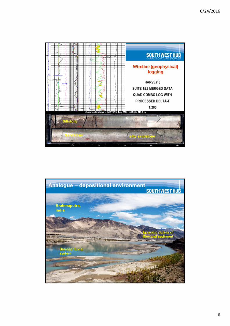
6/24/2016

6

Wireline (geophysical)

logging

Sandstone

Siltstone

silty sandstone

Analogue – depositional environment

Brahmaputra,

India

Episodic pulses of

flow and sediment

Braided fluvial

system

6/24/2016

7

Analogue – Hawkesbury

Sandstone, NSW

Static model

Geophysics, geology, petrogeophysics

depositional analogue – construct 3D

static model

Next? Populate the model

Recap

Core analysis data

– rock properties

6/24/2016

8

Core analysis: selecting and cutting plugs

Core analyses

These rock property data

are used to populate the:

1. static and

2. dynamic models

6/24/2016

9

Harvey-2, -3 and -4,

summarised

relative clay

mineralogy,

as determined by

XRD

Baffles and reservoir

Harvey 3 –

Wonnerup

Member

– 1,519 m

SEM 100 µm

SEM 10

µm

Harvey 3

–

Yalgoru

p

Member

– 1,354

m

6/24/2016

10

Wonnerup

Sabina

Yalgorup

F10 Fault

Western Fault

“Greater AOI”

25x25=214mil

250x250=1.1mil

“GeoGrid”

@ 25x25x1m

= ~166 mil cells

Area includes

all 4 wells.

“Sector Model”

@ 25x25x1m

= ~0.8 mil cells

(500mx500m)

“Sector Model”

Area Vs Cell Size

Aim for ~1 mil cells.

No Faults & No Wells.

Porosity

Grid : 250x250m

Layers : 1m Yalgorup

4m Wonnerup

Cells : 1.1milTop

Sabina

Top

Wonnerup

“F10”

Fault

H-2

H-4H-3

H-1

6/24/2016

11

Reference Case Injection Performance over 30 Years

01/20 01/22 01/24 01/26 01/28 01/30 01/32 01/34 01/36 01/38 01/40 01/42 01/44 01/46 01/48 01/50 01/520

50

100

150

200

250

300

350

400

450

500

550

600

650

700

750

800

CO

2 I

nje

cti

on

Ra

te (

ton

ne

s/d

ay

)

0

1MM

2MM

3MM

4MM

5MM

6MM

7MM

8MM

Cu

mu

lativ

e C

O2

Inje

cte

d (to

nn

es

)

CO2 Injection Rate Cumulative CO2 Injected

Maximum gas injection rate of ~700 tonnes/day

Probability Distribution of Injectivity after 30 Years

Single Well

Sample Johnson SB

Tonnes of CO2 After 30 Years

12111098765432

Probability

1

0.9

0.8

0.7

0.6

0.5

0.4

0.3

0.2

0.1

0

P50=5.9 million tonnes of CO2

P90=2.6 million tonnes of CO2

P10=9.6 million tonnes of CO2

Reference Case

6/24/2016

12

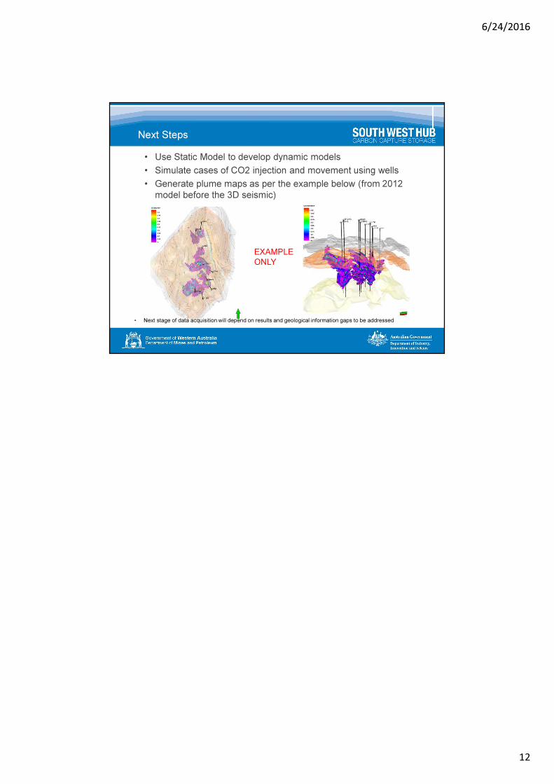
Next Steps

• Use Static Model to develop dynamic models

• Simulate cases of CO2 injection and movement using wells

• Generate plume maps as per the example below (from 2012

model before the 3D seismic)

EXAMPLE

ONLY

• Next stage of data acquisition will depend on results and geological information gaps to be addressed