Swaptions pricing under the single factor Hull-White Model...
65
Swaptions pricing under the single factor Hull-White Model through the Analytical formula and Finite Difference Methods Victor Lopez Lopez 1 Jan R¨ oman 2 1 Corresponding author, student of the Master of Science in Mathematics with focus in Financial Engineering at M¨ alardalen University. 2 Division of Applied Mathematics, M¨alardalen University.
Transcript of Swaptions pricing under the single factor Hull-White Model...

Swaptions pricing under the single factorHull-White Model through the Analytical
formula and Finite Difference Methods
Victor Lopez Lopez1 Jan Roman2
1Corresponding author, student of the Master of Science in Mathematics with focus inFinancial Engineering at Malardalen University.
2Division of Applied Mathematics, Malardalen University.


Abstract
Due to the interesting financial moment we are living, my motivations to writethis Master thesis has mostly been the behavior of interest rates and modelsthat can be used predict them. Thus, in this dissertation I have presented theHull-White model and the way to calibrate it against market data so it can beused to price interest rate derivatives. The reader can find both theoretical andpractical presentations and examples along with the code to program them byhim/herself.
I would like to take advantage of the situation and thank Jan Roman as Ihave relied through all this work on his lessons at Malardalens University. Thus,I would like to refer the reader to his work in the references [1] and [7] whenseeking for any deeper knowledge in this topic.

Contents
1 Introduction 4
2 Interest rate derivatives 52.1 Bonds, FRN and FRA . . . . . . . . . . . . . . . . . . . . . . . . 62.2 Swaps . . . . . . . . . . . . . . . . . . . . . . . . . . . . . . . . . 92.3 Swaptions . . . . . . . . . . . . . . . . . . . . . . . . . . . . . . . 122.4 Interest rate derivatives pricing . . . . . . . . . . . . . . . . . . . 122.5 Martingale modeling . . . . . . . . . . . . . . . . . . . . . . . . . 13
2.5.1 Affine Term structure . . . . . . . . . . . . . . . . . . . . 132.5.2 ATS models . . . . . . . . . . . . . . . . . . . . . . . . . . 14
3 Hull-White Model 153.1 Solving the Hull-White PDE to price Zero-Coupon bonds through
the Finite Difference Method . . . . . . . . . . . . . . . . . . . . 163.1.1 Boundary conditions . . . . . . . . . . . . . . . . . . . . . 19
3.2 Practical example of Zero-Coupon bonds pricing under Hull-Whiteby Crank-Nicolson Finite Difference Method using Python . . . . 19
3.3 Pricing European Swaptions under the Hull-White model . . . . 193.3.1 Practical example of Pricing European Swaptions under
Hull-White analytical formula using Python . . . . . . . . 21
4 Black-76 model 234.1 Pricing European Swaptions under Black-76 . . . . . . . . . . . . 23
4.1.1 Black-Normal model . . . . . . . . . . . . . . . . . . . . . 244.1.2 Practical example of Pricing European Swaptions under
Normal-Black using Visual Basic Application on MicrosoftExcel . . . . . . . . . . . . . . . . . . . . . . . . . . . . . 25
5 Calibration of the Hull-White model and results 265.0.1 Calibration of the Hull-White model. Practical example
using Python . . . . . . . . . . . . . . . . . . . . . . . . . 265.1 Risk measures. The Greeks . . . . . . . . . . . . . . . . . . . . . 27
5.1.1 Results . . . . . . . . . . . . . . . . . . . . . . . . . . . . 28
6 Conclusion 32
7 Fulfillment of thesis objectives 33
8 References 35
9 Appendix 1: Hull-White PDE solution by Finite DifferenceMethod (Crank-Nicolson) to price Zero-Coupon bonds. Pythoncode 36
2

10 Appendix 2: Pricing Swaptions under Hull-White using theAnalytical formula. Python code 41
11 Appendix 3: Pricing Swaptions under Black-76 and Normal-Black. VBA code 47
12 Appendix 4: Calibration of Hull-White Swaption prices. Pythoncode 53
13 Appendix 5: Figures 61
3

1 Introduction
Since the beginning of the crisis that started with the crash of Lehman-Brothersin 2008 the financial world has started to change very sharply. The credit marketcollapsed and central banks all over the world decided to lower interest rateslevels and power up their printing machine engines to try to fix the situation.This fact forced the rates down even more until we got to a situation no onecould have imagined before, interest rates reached bellow-zero levels. Thatmeans someone will lend money to another person expecting to get a smalleramount back. A financial non-sense. From this moment on, the situation haswidened and negative levels are deeper every month and are spreading to almostall developed economies.
Because negative rates where unthinkable, many models to estimate themwere made according to the fact that they did not exist. They were basedupon log-normal distribution, which makes negative rates impossible to handle.Therefore, nowadays they do not work adjusted to reality anymore. However,there exists some models (usually Gaussian-models) that let rates reach negativelevels because they rely on normal distribution. Hull-White’s Vacicek extensionis one of them and this dissertation will try to explain how to utilize it to priceSwaptions as these instruments can be used to calibrate the model against mar-ket data so it can price interest rate derivatives according to reality.
Thus, interest rates and their derivatives will be introduced in the first partof this work, followed by the explanation of the Hull-White model and twodifferent ways to find its solution (analytically and through numerical methods).Afterwards, the Black-76 model will be shown as it can be used to calibrateHull-White. Finally the calibration method and the results will be presented.Practical examples will be given in every section so the reader can see theusefulness of this model by him/herself.
4

2 Interest rate derivatives
Interest rates are probably the most important financial instrument as theydetermine the life of millions of people around the globe. Therefore, we can finda bunch of different interest rate derivatives in the market. In Figure 1 we finda classification of the most important fixed income securities. The table hasbeen taken from Roman, J. 2015[1].
Figure 1: Classification of interest rates derivatives. Roman, J. 2015[1]
Because interest rates usually mean periodic payments, to price them wehave to study their cash flows. Hence, the first thing to keep in mind whenvaluing cash flows is the moment in time in which they are treated, since wecan analyze both their future and present value. To evaluate the present valueof a cash flow that will happen in the future, we need to discount it first. Themost important methods to discount interest rates are:
• Simple compounding:
p(t) =1
1 + trsimple(t)
• Periodically compounding:
p(t) =1(
1 +rf (t)
f
)ft• Continuous compounding:
p(t) = e−rt
Where p(t) is the prize of a zero coupon at time t, f is the frequency of pay-ments per year and r is the interest rate. If we have enough instruments fromthe market with different maturities we can create a discount curve. A discountcurve is a function of time in which we have the future value of a product over
5

time and can be used to discount cash flows. The discount curve is created outof the most liquid interest rate instruments that we could find in the market.Usually these are deposits from 1 day to 3 months, FRA (Forward Rate Agree-ment) from 3 months to 2 years and Swaps from 2 years on. The formulas todiscount these 3 types of products are as follows:
• Over-Night Deposit:
DO/N =1
1 + rO/Ni
dO/N
360
• Tomorrow-Night Deposit:
DT/N =DO/N
1 + rT/Ni
dT/N
360
• Deposits:
Di =DT/N
1 + rparidi
360
• FRA:
DFRAi =
DFRAi−1
1 + rFRAidFRAi
360
• Swaps:
DT =DT/N − rparT
∑T−1t=1 YtDt
1 + YT rparT
With D being the discount factors of each product, d the length of the productin days, and rpar the Swap rate.
The discount curve for the data in Figure 24 of the Appendix 5 is shown inFigure 21 of the Appendix 5.
The process of creating an interest rate (yield) curve is called bootstrapping.Taking the logarithm of the discount factors with negative sign and dividing itby the amount of days that the instrument lasts we can get the Zero rates.Thus, we can construct an interest rate curve as the one shown in Figure 2,where we have the Zero rates, Swap rates and Forward rates for the data givenin Figure 24 of the Appendix 5.
2.1 Bonds, FRN and FRA
Bonds are the most common fixed-income security. They are defined as a con-tract in which the bond buyer agrees to lend an amount of money to the issuer inexchange to receive interest payments periodically (known as coupons) and theprincipal at maturity. The price of a bond as a function to the yield-to-maturityis shown as:
P =N
(1 + y)T+
n∑i=1
C
(1 + y)ti
6

Figure 2: Forward rates, Zero rates and Swap rates curve of the data given inFigure 24 of Appendix 5
where N is the nominal, y is the yield-to-maturity and C is the amount of thecoupon (C = cN). The present value of a bond is described by the followingequation:
PV (y, f) =
(1 +
y
f
)−Tf{N +
C
y
[(1 +
y
f
)M− 1
]}with f equal to the frequency of the payment per year and M being the numberof remaining cash flows and T the time to maturity.
There exist many different kinds of bonds like callable/putable (options onbonds), convertible (issued by companies, can be converted into stock), bulletbonds, etc. However, as most of interest rates derivatives can be seen as a seriesof Zero-Coupons bond, Swaps among them, in this dissertation we will focus onthe study of this kind of bonds.
A Zero-Coupon bond is a bond that has just one single payment at maturitymade out of the principal plus (or minus) the interest rates, none intermedi-ate coupons will happen. They are of great importance as they can be usedto discount and price interest rates derivatives. The idea under Zero-Couponpricing is taking all individual cash flows as if they where Zero-Coupon bonds.The evaluation of these cash flows is made using a yield curve or the discountfunction. This way of valuing interest rates derivatives is very popular especiallywhen pricing OTC (Over The Counter) instruments. In Figure 3 we can seehow a bond with several coupons can be seen as a sum of Zero-Coupon bonds.
Furthermore, another important interest rates instruments are notes. A
7

Figure 3: Bond scheme with several coupons vs Zero-Coupon bonds
note is similar to a bond with the difference that it has a shorter lifetime. Noteslifetime is usually between one and ten years, while bonds life is normally longer.Within notes, we can find the so-called Floating Rate Notes. The FRN are avery used financial instrument. They are quoted as a percentage of a notional,like bonds, however, FRN have reset dates. Every coupon date, the rate is resetin line with a money market reference, typically LIBOR, plus a fixed spread.The credit quality of the issuer is of great importance when pricing FRN, sinceif we wanted to trade it in the secondary market, the fixed spread should beshifted in case the rating of the issuer drops. Thus, when discounting, we haveto keep in mind the issuer discount curve p(0, i), where i is the current time.
P =
N∑i=1
[L(i− 1, i) + S]p(0, i) + p(0, N)
will be the price of an FRN, where we discount the sum of LIBOR L(i− 1) atthe previous coupon payment plus the spread S by the issuer discount to nextcoupon date i. We can estimate p(0, i) by the following formula:
p(0, i) =p(0, i− 1)
1 + L(i− 1, i) +Q
8

where Q is a measure of the credit quality of the issuer known as par floaterspread which changes over time. For the case where Q = S we have that theFRN is traded at par. The spread over the LIBOR paid in order to make theFRN price at par is known as Discount Margin or Effective LIBOR spread andis calculated by iterations looking for the value of M in:
p =
(Lnext + S) +∑Ni−1
L+ S
(1 + L+M)i+
1
(1 + L+M)N
1 + L∗ +M
where p is the bond price, L∗ is the stub LIBOR coupon to next coupon date,Lnext is the next LIBOR payment and M is the discount margin which valuewe are looking for.
The last instruments we will study in this section are the Forward RateAgreements. FRA are interest rate derivatives starting in the future withoutexchanging the principal. Thus, just differences on interest rates are tradedwhen the instrument matures. They are an agreement to borrow (or lend) anotional for a period of time at an agreed interest rate. This interest rate canbe lower or higher than the market rate set by the contract and so, it can beused to hedge or speculate. For example, if the rate of the FRA is set at 5% in6 months on LIBOR for 3 months and LIBOR stays at a lower level, lets say4%, the issuer of the FRA must pay the difference to the buyer for a 3 monthsperiod. They are very similar to Swaps (presented in Section 2.2) with thecontrast that FRA pay the difference of interest rates only once, at maturity.The value of an FRA is calculated as:
P = NτL(t, T )−K1 + τL(t, T )
where t and T are start of the FRA and maturity respectively, K is the striketo be paid at t2, and τ = T − t in days (taking a year as 360 days). FRA atpar (K = L) are standardized nowadays because of its importance and are setas three month contracts between the famous IMM-days (third Wednesday ofMarch, June, September and December).
2.2 Swaps
Swaps are among the most popular financial products that can be found inthe market nowadays and are the most traded ones by far when talking aboutfixed-income derivatives. A Swap is an agreement by which two counter-partiesexchange financial instruments periodically, mainly cash flows on a notional. Inthis case, one party agrees to pay the other party a cash flow equal to a fix rateon the notional and the other party pays floating rates cash flows (usually basedon an interest rate index like LIBOR or EURIBOR) on the same notional inexchange. It is easy to see how one can use it either to cover against possiblefluctuations on interest rates or to speculate under the idea of predicting thesefluctuations. Generally these agreements are taken by companies or financialinstitutions with the idea of hedging possible losses from rates.
9

The present value of a Swap can be easily calculated discounting the pay-ments and since commonly the notional is the same for both counter-parties, itwill not be exchanged. These payments will be done periodically at previouslydetermined dates called reset dates (monthly, every semester, annually, etc). Tobe able to price them, we have to calculate both the discounted fixed paymentsand the floating ones. However, as we can not determine the floating paymentsat the start of the contract, we have to estimate them calculating the forwardrate for each respective payment date of bonds traded in the market with similarmaturities.
Each of these cash flows is discounted by the Zero-Coupon rate for the dateof the payment given by the yield curve from the market. Therefore, we cantreat the interest rate Swap as a series of Zero-Coupon bonds from a reset dateto the following one. The sum of all these Zero-Coupons will be the presentvalue of the floating leg of the Swap.
Furthermore, the Swap fixed rate will be set at a level that will make thefixed payments have the same present value as that of the floating leg. Thus,at the time of the agreement, there will be no advantage for any of the parties.However, during the life of the Swap, the PV of the floating flows will vary asthe interest rates fluctuate and both legs will not have the same value when theSwap matures. The structure of a Swap with 2 payment dates starting in thefuture is shown in Figure 4.
Figure 4: Payment structure of a 2 periods Swap.
Letting ∆i be the length of the period between Ti−1 and Ti in days and DTi
be the discounting factor at time Ti that is calculated as follows
D(Ti) =D(Ti−1)
1 + ∆iFi
the forward rate of a single currency Swap for the period [Ti−1, Ti] will be:
Fi =D(Ti−1)/D(Ti)− 1
∆i
10

where Ti represent the reset days of the Swap. Now, letting Li be the marketrate (LIBOR) we can see that the value today of the floating cash flow ∆iLi is:
∆iFiD(Ti) = ∆iD(Ti−1)−D(Ti)
∆iD(Ti)D(Ti) = D(Ti−1)−D(Ti)
Thus, if we add up the values for all the life of the Swap we will get the wholefloating leg as:
n∑i=1
∆iFiD(Ti) =
n∑i=1
D(Ti−1)−D(Ti) = D(T0)−D(Tn) = 1−D(Tn)
And the value of the fixed leg with rate C is
C
n∑i=1
∆iD(Ti)
Thus, to get the fair Swap rate at maturity Tn, we must find the value Cn forthe following equality
Cn
n∑i=1
∆iD(Ti) = 1−D(Tn)
This rate that equals both legs at the time when the contract is made is knownas par rate.
Lets now study the case when we use bonds for discounting. Thus, we willbe using the forward rate
f(ti−1, ti) =p(0, ti)− p(0, ti−1)
∆ip(0, ti)
and following the steps given above the whole value of the floating leg is asfollows:
N∑i=n+1
∆if(t, T )p(t, Ti−1) =
N−1∑i=n
[p(t, ti)− p(t, ti+1)] = pn(t)− pN (t)
On the other hand the fixed leg will be equal to
C
N∑i−n+1
∆ipi(t)
Hence, the total value of the payer Swap is
pn(t)− pN (t)− CN∑
i=n+1
∆ipi(t)
11

that must be equal to 0 in order to be at par. Therefore, the forward Swap rateRNn (t) is equal to
RNn (t) = C =pn(t)− pN (t)∑Ni=n+1 ∆ipi(t)
(1)
The process Skn =∑Ni=n+1 ∆ipi(t) is known as the accrual factor or value of a
basis point (can be found under the acronyms DV01 and PV01 ).
2.3 Swaptions
A Swaption is an option to enter into a Swap. Similar to stock options, thereexists both call and put possibilities, however, here they are defined as payerand receiver Swaptions. A payer Swaption is the right but not the obligation ofentering into a Swap in a given date, paying the fixed rate (Strike) and receivingthe floating rate. On the other hand, a receiver Swaption is the opposite, theright but not the obligation to enter into a Swap receiving the fixed rate andpaying the floating rate in a given date. There exists also both European andAmerican Swaptions. Like in the European options, a Swaption can only beexercised at maturity. However, in contrast to options, an American Swaptioncan just be exercised on cash flow dates, not continuously. There also exists ahybrid of both American and European Swaptions that can only be exercisedat reset dates, these are called mid-Atlantic or Bermudan.
We have then that a payer Swaption is a put option on a fixed rate bondwith strike price equal to the face value of the bond. On the other hand, areceiver Swaption is a call option on a fixed rate bond with strike price equal tothe face value of the bond.
2.4 Interest rate derivatives pricing
To understand the mathematical procedure of pricing interest rate derivatives,we have to understand that the short rate process is typically set under the Pprobability. The short rate process is defined as follows:
dr(t) = µ(t, r(t))dt+ σ(t, r(t))dW (t) (2)
where dW is a Wiener process. dW will be used every time we refer to a Wienerprocess from here on.
We will find that (2) is determined by the General Term Structure equation(3), which defines the short rates behavior during time.
∂FT
∂t+ {µ(t, r)− λ(t, r)σ(t)}∂F
T
∂r+
1
2σ2 ∂
2FT
∂r2− r(t)FT = 0
F (r, T, T ) = Φ(r)
(3)
12
In this partial differential equation we find that the drift of the short rate (µ−λσ) is defined under the martingale measure Q. Under martingale probabilitymeasures, if we have a stochastic process X with information known up to timet, the expected future value of X(t+s) will be equal to X(t). Therefore, we willneed to specify the r-dynamics (2) (that are set under P ) on this martingalemeasure Q. This method is called martingale modeling and we can find a bunchof different models of this kind.
2.5 Martingale modeling
When martingale modeling, it happens that some of these models have a par-ticular term structure that will eliminate most of the mathematical difficulty.These models are said to have an Affine Term structure. Therefore, the PDEswe will have to front when dealing with ATS models are easier to solve.
2.5.1 Affine Term structure
First, we will start describing what an Affine Term structure is:
If the term structure {p(t, T ); 0 ≤ t ≤ T ;T > 0} has the form p(t, T ) =F (r(t), t, T ) where
F (r, t, T ) = eA(t,T )−B(t,T )r (4)
and A and B are deterministic functions, then the model possess an Affine Termstructure. A model is said to have an ATS if the continuously compounded shortrate R(t, T ) is an ATS of the short rate r(t). This means that the process islinear plus a constant like:
R(t, T ) = α(t, T ) + β(t, T )r(t)
In this model α and β are deterministic functions of time.α(t, T ) =
A(t, T )
T − t
β(t, T ) =B(t, T )
T − t
Since having an ATS is so important when martingale modeling, we willdescribe how to know if we have an Affine Term structure. Assuming that wehave (2) under the Q probability measure, the process to check if our modelposses an ATS for the case of a Zero-Coupon bond is as follows (demonstrationof the calculations can be found in Roman 2015 pp[257-286]):
Substituting (4) in (3), we get
∂A(t, T )
∂t−{
1 +∂B(t, T )
∂t
}r(t)− µ(t, r(t))B(t, T ) +
1
2σ2(t, r(t))B2(t, T ) = 0
13

Furthermore, applying the Zero-Coupon bond boundary condition F (r, T, T ) =1 in (4) we get the boundary condition for the equation above as 1 = eA(T,T )−B(T,T )r.Thus A(T, T )−B(T, T )r must be 0 and then
A(T, T ) = B(T, T ) = 0
We can already realize how the calculations are simplified when using ATS.Furthermore, analyzing that result, we see that if µ and σ2 are both affine, theequation becomes a Separable Differential Equation. Thus, we can assume µ(t, r) = a(t)r + b(t)
σ2(t, r) = c(t)r + d(t)
and so, substituting above, we have:
∂A(t, T )
∂t−{
1+∂B(t, T )
∂t
}r(t)−{a(t)r+b(t)}B(t, T )+
1
2{c(t)r+d(t)}B2(t, T ) = 0
that can be separated as
∂A(t, T )
∂t− b(t)B(t, T ) +
1
2d(t)B2(t, T ) = 0
∂B(t, T )
∂t+ a(t)B(t, T )− 1
2c(t)B2(t, T ) = −1
A(T, T ) = B(T, T ) = 0
(5)
Solving this Separable Differential Equation we can analyze the Q-dynamics ondr(t) and therefore, find the derivatives prices.
2.5.2 ATS models
We can find a bunch of different ATS models. Among the most important oneswe can find, along with their short rate process, the followings:
• Vasicek: dr = (b− ar)dt+ σdW
• Cox-Ingeroll-Ross (CIR): dr = a(b− r)dr + σ√rdW
• Black-Derman-Toy: dr = a(t)rdt+ σ(t)rdW
• Ho-Lee: dr = a(t)dt+ σ(t)dW
• Hull-White: dr = (b(t)− a(t)r)dt+ σ(t)dW (t)
In this dissertation we will focus on the study of the latter.
14

3 Hull-White Model
This model was developed by John Hull and Allan White in 1990 in their article”Pricing Interest-Rate Derivative Securities”[3]. As they defined it, it is anextension of the Vasicek model. However, in H-W the parameters are time-dependent, what increases the possibility of calibrating them with respect tomarket data. The Hull-White model is growing in importance lately due to thereason that it allows the interest rates to be negative while we will not find thisfeature in many other models. In the past, when the people surrounding thefinancial world thought of negative interest rates as something impossible, itwas criticized for the same reason. However, nowadays reality is quite differentand negative rates are all over the market. Furthermore, many specialists onthe matter say they are here to stay.
The explanation of why negative interest rates are possible in this model isthat the short rate in Hull-White is normally distributed (it is a so-called Gaus-sian model). On the other hand, for example, Black-76 (the most commonlyutilized model) has a log-normal distribution. Hence, in these models negativevalues for the rates are not allowed since the logarithm of a non-positive numberis not defined. We find that in Black’s model volatility is defined as:
dF = σBFdW F (0) = f
where σB is the implied Black volatility. As we have log-normality we will needto calculate log(F/K) for d1 and d2 in the Black formula for pricing interestrates derivatives than can be found in Black, F. 1976 [5]. Therefore, the modelis unusable for non-positive values of F . Nevertheless, in Gaussian models:
dF = σNFdW F (0) = f
where σN is the normal volatility. Furthermore, another remarkable feature ofthe Hull-White model is that it allows us to use trinomial trees (lattice), as well.
The Hull-White stochastic process is defined as
dr = (θ(t)− a(t)r)dt+ σ(t)dW (t)
It is easy to see that it follows the dynamics presented in (2). Furthermore, it isan special case which includes mean-reversion. Here θ is a deterministic functionof time and will be calibrated against the theoretical yield curve. On the otherhand, a and σ should be chosen to reflect the current and future volatilitiesof the short-term-interest rate. So like in Vasicek model they can be fitted tothe current term structure of interest rates and the current term structure ofinterest-rate volatility respectively. a is the mean reverting parameter, and isdefined in a way in which the drift of the process will be negative for valuesof r greater than θ/a and vice-versa. We can appreciate it better recalling theTerm Structure equation with the Zero Coupon boundary condition and theHull-White r-dynamics:
15

∂FT
∂t+ {θ(t)− a(t)r(t)}∂F
T
∂r+
1
2σ2 ∂
2FT
∂r2− r(t)FT = 0
F (r, T, T ) = 1
(6)
We see that µ(t, r)− λ(t, r)σ(t) = θ(t)− a(t)r(t) and so, the drift includes themarket price of risk and the volatility that should be calibrated against realdata. The analytical solution for the short rates in this model is as follows:
r(t) = r(s)e−a(t−s) +
∫ t
s
e−a(t−u)θ(u)du+ σ
∫ t
s
e−a(t−u)dW (u)
where
θ(t) = f(0, T ) + af(0, T ) +σ2
2a(1− e−aT )
and the Zero-Coupon bond price:
p(t, T ) = A(t, T )eB(t,T )r(t) (7)
A(t, T ) =p(0, T )
p(0, t)exp
{B(t, T )f(0, t)− σ2
4aB(t, T )2(1− e−2at)
}B(t, T ) =
1
a(1− e−a(T−t))
with f(0, t) being the forward rate and p(0, t) the price of a bond starting todaywith maturity at time t. Calculations to these solutions can be found in Roman2015 [1] p.309-316.
3.1 Solving the Hull-White PDE to price Zero-Couponbonds through the Finite Difference Method
In this dissertation we will show the procedure to price Zero-Coupon bonds solv-ing the Hull-White PDE through the Finite Difference Method, in particular,Crank-Nicolson.
There are three types of finite difference methods to solve PDE’s. Theexplicit difference method, that follows backward differences to approximatethe derivatives; the implicit difference method, that follows forward differences;and the Crank-Nicolson (mixed) method that combines both of them as can beseen in Figure 5 taken from Roman, J. 2014[4]. Therefore, in the mixed method,we use information both from t and t − ∆t and furthermore, the accuracy isgreater.
• Forward difference:∂f(x, y)
∂y∼=f(x, y + δy)− f(x, y)
δywith rate of convergence O(∆x+ ∆y)
• Backward difference:∂f(x, y)
∂y∼=f(x, y)− f(x, y − δy)
δywith rate of convergence O(∆x2 + ∆y)
16

• Central difference:∂f(x, y)
∂y∼=f(x, y + δy)− f(x, y − δy)
2δywith rate of convergence O(∆x2 + ∆(y/2)2)
• Second central difference:∂2f(x, y)
∂y2∼=f(x, y + δy)− 2f(x, y) + f(x, y − δy)
δ2y
with rate of convergence O(∆y4)
Figure 5: Finite difference methods information schema, Roman J. 2015, [4].
To solve the PDE in (6) through Crank-Nicolson we then need to define agrid with the rates as rows and time as columns. The idea behind this gridis to discretise these two variables in N pieces of h length equal to dr and Tpieces of k length equal to dt. Therefore, applying the central and second centraldifferences to both variables we get
uij = u(ri, tj)
∂u(ri, tj)
∂t=uij+1 − uij−1
2k
∂u(ri, tj)
∂r=ui+1j − ui−1j
2h
17

∂2u(ri, tj)
∂r2=ui+1j + ui−1j − 2uij
h2
Now, applying these Crank-Nicolson equalities to the Hull-White term-structureequation (6) we have:
∂uij∂t
= riuij − {θ(t)− a(t)r(t)}ui+1j − ui−1j
2h− 1
2σ2ui+1j + ui−1j − 2uij
h2
that can be realigned to give the multipliers of each uij
∂uij∂t
=
(− σ2
2h2+{θ(t)− a(t)r(t)}
2h
)ui−1j+
(σ2
h2+ri
)uij−
(σ2
2h2+{θ(t)− a(t)r(t)}
2h
)ui+1j
Thus, letting:
Pd = − σ2
2h2+{θ(t)− a(t)r(t)}
2h
Pm =σ2
h2+ ri (8)
Pu = − σ2
2h2− {θ(t)− a(t)r(t)}
2hwe can perform the following matrix where tj = jk; j = 0, 1, 2, ..., T and ri =ih; i = 0, 1, 2, ..., N
A =
Pm(r0, tj) Pu(r0, tj) 0 0 0 .... 0Pd(r1, tj) Pm(r1, tj) Pu(r1, tj) 0 0 .... :
0 Pd(r2, tj) Pm(r2, tj) Pu(r2, tj) 0 .... :0 0 Pd(r3, tj) Pm(r3, tj) Pu(r3, tj) .... :: : : : : : :0 0 0 .... 0 Pd(rN , tj) Pm(rN , tj)
that will define the behavior of the rates every time-step k passes. Letting avector u represent the rates at time j, following Crank-Nicolson, we will havethe functions that define increments in rates from j to j + 1 as:
uj+1 − ujk
=A(tj)uj + A(tj+1)uj+1
2
that will be solved as:
uj =
(I +
k
2A(tj)
)−1(I− k
2A(tj+1)
)uj+1
Reprocessing this calculations starting from maturity backwards for all time-steps and organizing u in a matrix we will get the solution for the PDE. Note thatin the case of Zero-Coupon bonds we should start with the boundary conditionuT = 1 for all i since the value of a Zero-coupon bond at maturity will equal 1.The code of a Python application to compute this FDM process can be foundin the Appendix 1.
18

3.1.1 Boundary conditions
As we are pricing Zero-Coupon bonds, at maturity our derivatives will be worth1. Therefore, the first boundary condition for this system of equations will beuT = 1 for all rates.
On the other hand,∂2u(ri, tj)
∂r2= 0 is used as boundary conditions at the
first step of the grid (Pd(r0, tj), Pm(r0, tj) and Pu(r0, tj)).
3.2 Practical example of Zero-Coupon bonds pricing un-der Hull-White by Crank-Nicolson Finite DifferenceMethod using Python
In this section we will show a practical example of the process to solve the Hull-White PDE (6) by the Crank-Nicolson Finite Difference Method in Python. Thewhole code to compute this application can be found in Appendix 1. The setvalues for this practical example are σ = 0.02, θ = 0.02, a = 0.01 and themaximum and minimum values to define the C-N grid of r are −0.015 and 0.3respectively. The grid has been created as it has a size of 63x333 in which weplot the rate level on the vertical axis and the time to maturity on the horizontalaxis. To define the pieces in which the grid will be divided we have used the
following formulas M =rmax − rmin
drand N =
1
dtwhere dr and dt are the
size of each piece for rates and time and M and N are the number of piecesin which the axis are divided. After defining the boundary conditions givenin Subsection 3.1.1 we can create the matrix A(T − 1) in Section 3.1 applying(8) for each time-step. The first rows and columns of this matrix are shown inFigure 22 of the Appendix 5. Once this step is performed, we set A(T −2) to beable to calculate uT−2, that will be the second column of our Crank-Nicholsongrid (the first column is set equal to 1 as the boundary condition at maturity).Performing this process from maturity time to the first time-step of the bond lifewe complete the Crank-Nicholson grid (Figures 6 and 7). This grid representsthe different values for Zero-Coupon bonds for rates range (−0.015, 0.3) frommaturity to bond start. Each vector of the grid can be used as a discountingfunction to discount financial instruments for its respective risk-free rate.
3.3 Pricing European Swaptions under the Hull-Whitemodel
Following Jamshidian [6] if we have ”a term structure that is completely deter-mined by the value of the instantaneous interest rate r(t) that follows a mean-reverting Gaussian process, [...] an option on a portfolio of pure discount bondsdecomposes into a portfolio of options on the individual discount bonds in theportfolio.” Hence, we can think of the European Swaption as a sum of Europeanoptions on Zero-Coupon bonds. This method is called Jamshidian’s decomposi-
19

Figure 6: Crank-Nicolson grid for Zero-Coupon bonds
Figure 7: Crank-Nicolson heat map for Zero-Coupon bonds
tion in his honor, and is mathematically explained as follows:
max
[ n∑i=1
Cip(r, t, si)−K, 0]
=
n∑i=1
Ci max
[p(r, t, si)−Ki, 0
](9)
20

The method is the following:Consider a European Swaption with strike rate K, maturity T and nominal Lwith payment dates Ti for i = 1, ..., n. Since the value of a floating rate bondis worth its face value, we can take it as an option on a bond paying Ci = Ksi
with strike price L. This option will be exercised when r(T ) < r∗ where r∗ isthe solution to
L =
n∑i=1
Cip(r∗, T, Ti)
This means that L is taken as a sum of discounted flows Ci for a short rate r∗ attime T . To find the value of r∗ we have to discount all the Swap cash-flows, sumthem up and let the sum be equal to the notional. We have to use the Newton-Raphson algorithm to follow this calculation r∗, that will be the correspondentlevel of r for that equality to happen. The Newton-Raphson algorithm has beentaken from the imported Python library scypi.optimization. Once r∗ is found,we have to calculate the discounted cash-flows substituting it in the discountingfactor e−r∆t and let them be the strike prices of our call options on Swaps.Afterwards, we calculate the payoff of the call options on the cash-flows withthe strike price mentioned and sum them up. The payoff of this sum of optionswill thus be
max
[ n∑i=1
Cip(r, T, Ti)− L, 0]
which using (10) we find is equivalent to
n∑i=1
Ci max
[p(r, T, Ti)− Li, 0
]where Li = p(r∗, T, Ti). Therefore, the Swaption is calculated as the sum of noptions on discounted bonds with the exercise price of the ith option equal to Li.
After the price of a European Swaption under the Hull-White model is cal-culated, we have to calibrate it against the market data. Usually this calibrationmethod is carried out taking the target prices to match the ones given by theBlack-76 or Normal-Black models and trying to get as close as possible to them.Further information on this method can be found in sections 4 and 5.
3.3.1 Practical example of Pricing European Swaptions under Hull-White analytical formula using Python
A practical example on pricing European payer Swaptions under Hull-Whitewill using the analytical formula be given in this section. The whole code ofthe Python application can be found in the Appendix 2. The inputs have beenset as r = 0.01%, σ = 1%, a = 0.05, Swap tenors={1, 2, 3, 4, 5, 7, 10, 12, 15, 20}and Swaption maturities={1/12, 4/12, 6/12, 1, 2, 3, 4, 5, 7, 10, 20} in years. Fre-quency has been let as one per year to simplify calculations.
21

As it has been presented above, the Hull-White analytical solution is givenby (7). The first step is therefore, to calculate the discount factors applyingit to the Zero bonds that are given in the Figure 24 of the Appendix 5. Oncewe have the discount factors we can calculate the floating and fixed legs of theSwaps and the Swap rates as it is shown in Subsection 2.2. Afterwards, we canfind the forward Swap rates calculating
RNn (t) =pn(t)− pN (t)∑Ni−n+1 ∆ipi(t)
At this point we have to apply Jamshidian as shown in the previous section. Todo so, we calculate the cash-flows given by the discounted fixed rate paymentsand make them be equal to the strike rate. In this practical example, the strikerate has been set 1 basis point bellow the correspondent forward Swap rate.Then, applying the Newton-Raphson algorithm we get r∗ and we can use it toget the value of the strike rate of our options in Swaps. The Swaption valuationis straightforward then, and it is done by summing up all the options. In Figure8 we can find the European payer Swaption prices in percentage for the Swaptenors in rows and Swaption maturities in columns given above.
Figure 8: Swaption prices under Hull-White model in %
22
4 Black-76 model
The Black-76 model is a modification of the original Black-Scholes formula madeby Black in 1976 [5] (hence its name) for valuing interest rate derivatives. Itis among the most used models nowadays to price this kind of instrumentsdue to its simplicity in comparison with more complicated models like the onespresented in Subsection 2.3. The European call and put prices under Black-76are as follows:
C = e−rT [FN(d1)−KN(d2)]
P = e−rT [KN(−d2)− FN(−d1)]
where
d1 =ln(F/K) + (σ2/2)T
σ√T
d2 = d1 − σ√T
F refers to the underlying of the derivative and K to the strike price. It is easyto see that for the case of F (T ) = F0e
rT Black-76 becomes Black-Scholes, so wecan think of it as a generalization of the original B-S formula.
However, this model has its weaknesses. As in Black-Scholes, it assumesthat the underlying follows a log-normal distribution, which makes negativerates impossible to analyze.
4.1 Pricing European Swaptions under Black-76
Recalling the explanation given in Subsection 2.3 and the European call formulaabove, we can define a payer European Swaption as the contract given by:
PNn (t, RNn (Tn),K) = SNn (Tn) max{RNn (Tn)−K, 0}
Letting SNn be the numeraire, a payer Swaption will be a call option on RNnwith strike rate K. Under the Black-76 formula, the value of this contract is asfollows:
PNn (t) = SNn (t){RNn (t)N(d1)−KN(d2)} (10)
where
d1 =ln{R
Nn (t)K }+ 1
2σ2n,N (Tn − t)
σn,N√Tn − t
d2 = d1 − σn,N√Tn − t
with σn,N being the Black volatility. As it is the volatility implied by the Blackformula, it is also known as implied Black volatility.
Now, using (1) we can transform (10) to
PNn (t) =pn(t)− pN (t)
RNn (t){RNn (t)N(d1)−KN(d2)}
23

and doing some algebra we can calculate the annuity as
pn(t)− pN (t)
RNn (t)=p(t, tn)[1− p(tn, tN )]
RNn (t)=
p(t, tn)
{1− 1
(1 + f(tn, tN ))tN−tn
}RNn (t)
Thus, we can finally get the Black-76 formulas for payer (PS) and receiverSwaption (RS) as:
PS =
1− 1
(1 + C/m)τm
Ce−rT [CN(d1)−KN(d2)]
RS =
1− 1
(1 + C/m)τm
Ce−rT [KN(−d2)− CN(−d1)]
where we let C be the forward Swap rate between n and N , m be the amount ofreset days per year, τ be the tenor of Swap (time between Swaption and Swapmaturities),
d1 =ln{CK }+ 1
2σ2T
σ√T
andd2 = d1 − σ
√T
4.1.1 Black-Normal model
As presented above, in a world with negative rates a log-normal model has itsdisadvantages. Therefore, we need to apply some transformations to the Black-76 model in order to be used with normality. This model is called Black-Normaland is basically Black-76 with Normal volatility. Prices for Swaptions under theBlack-Normal model are calculated as bellow:
PS =
1− 1
(1 + C/m)τm
Ce−rT
[(C −K)N(d) +
σ√T√
2πe−d
2/2
](11)
RS =
1− 1
(1 + C/m)τm
Ce−rT
[(K − C)N(d) +
σ√T√
2πe−d
2/2
](12)
with
d =C −Kσ√T
and the transformation between Normal volatility and Black volatility is givenby the next equality
σN = C
√2π
T
[2N
(σB√T
2
)− 1
]
24

where σN represents the Normal volatility and σB the Black volatility. In casethe reader is interested in going deeper in these equivalences they are referencedto Roman,J. 2015 [1] p.111 and p.444-446.
4.1.2 Practical example of Pricing European Swaptions under Normal-Black using Visual Basic Application on Microsoft Excel
In this section, a basic example of the theoretical explanation given above ofhow to value a European payer Swaption under Normal-Black is presented. Forthe calculations VBA on Ms Excel has been used and the full code to the modelcan be found in the Appendix 3.
In Figure 23 of the Appendix 5 we have the Quoted Normal Volatilitiesgiven by the market in Term/Term Swap/Swaption form up to 20 years. Thisinformation has been provided by Jan Roman and corresponds to the marketdata gathered by Swedbank at 2015-07-07. However, it can be found on financialinformation providers like Bloomberg or Reuters everyday.
Now we need to calculate the at-the-money forward rates to let them be ourSwap rates. To do so we have applied (1) on the bootstraped Swap rates thathave been shown in Figure 2 in Section 2.1. Following this process we havecreated the Swap rates matrix given in Figure 9, where we can find each andevery forward Swap rate at the same periods of time as we have the volatilitieswith columns representing Swaption maturity and rows being Swap tenors.
Figure 9: Forward Swap rates
Once we get to this point, we can apply the formula (11) for payer Swaptionto our data (or (12) in case we wanted to calculate the prices of the receiverSwaption). For this practical example we have applied the formula defined inAppendix 3 NormalSwaptionPricing (11) to an annual Swaption with risk-freerate r = 0.1%. The volatilities for each period are gotten from Figure 15 andSwap rates are provided in Figure 9. The strike rates have been set 0.01 pointsbelow the Swap rates by default for these calculations. The results can befound in Figure 10, which represent the prices in percentage for Swaptions inTerm/Term Swap/Swaption.
After we have calculated the Normal prices of European payer Swaptions forall the combinations of Swap Tenor and Swaption maturity that can be seen inthe matrix on Figure 10. This prices will be the ones we will use to calibrateour Hull-White model.
25
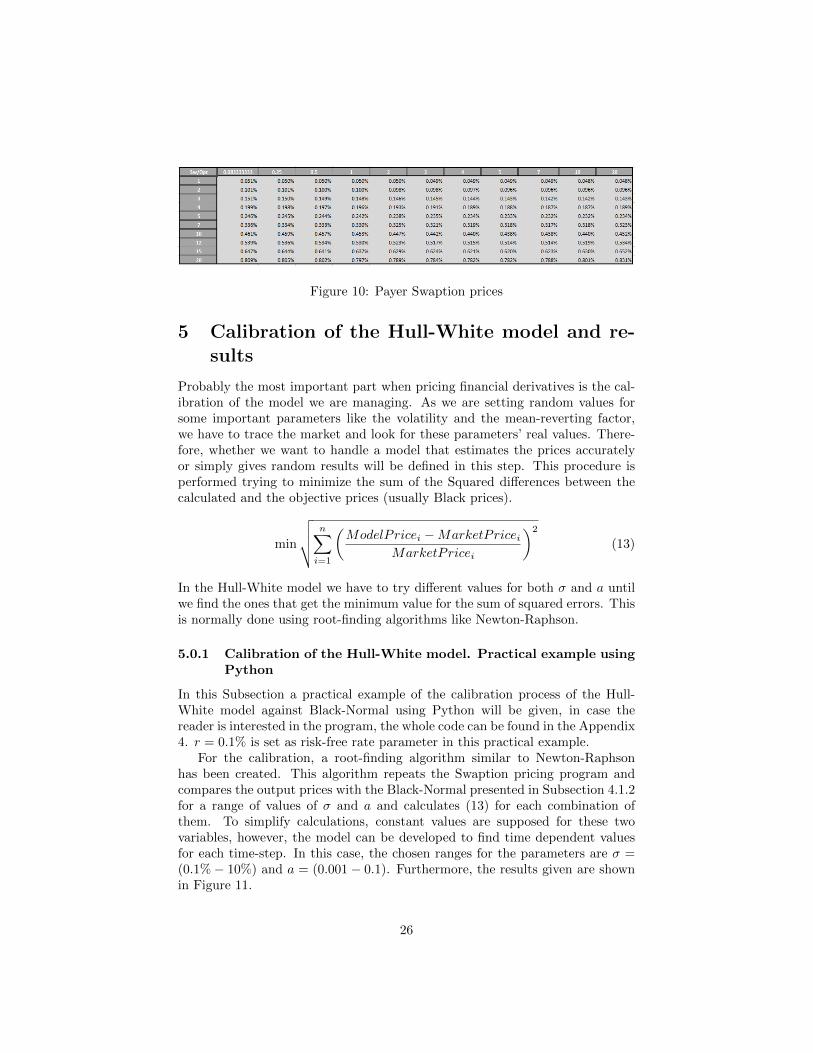
Figure 10: Payer Swaption prices
5 Calibration of the Hull-White model and re-sults
Probably the most important part when pricing financial derivatives is the cal-ibration of the model we are managing. As we are setting random values forsome important parameters like the volatility and the mean-reverting factor,we have to trace the market and look for these parameters’ real values. There-fore, whether we want to handle a model that estimates the prices accuratelyor simply gives random results will be defined in this step. This procedure isperformed trying to minimize the sum of the Squared differences between thecalculated and the objective prices (usually Black prices).
min
√√√√ n∑i=1
(ModelPricei −MarketPricei
MarketPricei
)2
(13)
In the Hull-White model we have to try different values for both σ and a untilwe find the ones that get the minimum value for the sum of squared errors. Thisis normally done using root-finding algorithms like Newton-Raphson.
5.0.1 Calibration of the Hull-White model. Practical example usingPython
In this Subsection a practical example of the calibration process of the Hull-White model against Black-Normal using Python will be given, in case thereader is interested in the program, the whole code can be found in the Appendix4. r = 0.1% is set as risk-free rate parameter in this practical example.
For the calibration, a root-finding algorithm similar to Newton-Raphsonhas been created. This algorithm repeats the Swaption pricing program andcompares the output prices with the Black-Normal presented in Subsection 4.1.2for a range of values of σ and a and calculates (13) for each combination ofthem. To simplify calculations, constant values are supposed for these twovariables, however, the model can be developed to find time dependent valuesfor each time-step. In this case, the chosen ranges for the parameters are σ =(0.1%− 10%) and a = (0.001− 0.1). Furthermore, the results given are shownin Figure 11.
26

Figure 11: Sum of squared errors for the range of values given for volatility andmean-reverting parameter
As it can be seen in Figure 11, the minimum error is reached at σ = 6.4%and a = 0.041. The calibrated prices for the Swaptions in Subsection 3.3.1 areshown in Figure 12.
Figure 12: Calibrated Swaption prices under Hull-White model in %
5.1 Risk measures. The Greeks
After calibration is done, we should measure risks from both models to comparethem. This process is done using the Greeks. The Greeks are different measuresof how much an instrument price varies when one of its variables changes. Usu-ally, the shift used in the Greeks calculations is 1/1000 of a basis point and theresult is then scaled to a one basis point shift (letting scale = 1000).The most
27

important Greeks are:
• Delta price: Shows the change in the theoretical price given a variation ofa unit in the price of the underlying.
∆price =∂(PV )
∂U=PV (U + h)− PV (U)
h∗ scale
• Delta yield: Shows the change in the present value, given a shift of onebasis point in the yield curve. Normally it is done adding 0.00001 tothe prices of the Zero-Coupon curve and giving scale the value 1000 i.e.shifting it by 1 basis point.
∆yield =[PV (r + h)− PV (r)
]∗ scale
• Gamma price: Shows the variation in Delta price, given a unit change inthe underlying.
Γprice =PV (U + 2h)− 2PV (U + h) + PV (U)
h2∗ scale
• Gamma yield: Shows the change in Delta yield given a basis point changein the yield curve. As in the Delta yield, 0.00001 is added to each nodeof the Zero-Coupon curve. However, in this case, as it is similar to takingthe square of the Delta yield, the scale will be 10002
Γyield =[PV (y + 2h)− 2PV (y + h) + PV (y)
]∗ scale
• Rho: Shows the change in the present value, given a shift of one basispoint in the repo curve.
ρ =[PV (rrepo + h)− PV (rrepo)
]∗ scale
• Theta: Shows the change in the present value given the valuation dateuntil the following calendar date.
Θ = PV (date)− PV (date+ 1)
• Vega: Shows the change in the present value given an shift in volatility of1%.
ν =[PV (σ + 0.01)− PV (σ)
]5.1.1 Results
Therefore, to compare the risks between both Normal-Black and Hull-Whitemodels, we have performed the Delta yield, Gamma yield and Vega to ourproducts. However, as the prices of the Swaptions are given in percentage andthe Greeks will take small values, a notional of 10.000.000 SEK has been set,
28

Figure 13: Black-Delta yield
Figure 14: HW-Delta yield
since it is a common amount for a Swaption contract. Doing so, the results willbe more understandable.
From Figures 13 and 14 we can affirm that for a Swap of tenor 20 yearswith a Swaption of 1 year, if the Zero-Coupons were shifted by 1 basis point,the price of the contract would change 207 SEK according to the Normal-Blackmodel and 352 SEK in the Hull-White program we have developed. Hence, thedifference in risks between the two models is very small (145 SEK) what is anacceptable amount when dealing with a contract of 10 million SEK.
Furthermore, traders would check the Gamma yield risk to be sure of howthe Delta yield would change given the same shift in the Zero-Coupon curve.In Figures 15 and 16 we have the values for this Greek.
Figure 15: Black-Gamma yield
The Gamma yield is thus, equal to −4.23 in the Normal-Black model and−8.51 in Hull-White, also very similar one to each other.
Finally, we will calculate Vega as the traders would analyze the possible risks
29

Figure 16: HW-Gamma yield
coming from changes in volatility. The results are shown in Figures 17 and 18.
Figure 17: Black-Vega
Figure 18: HW-Vega
Vega shows that the price of the Black-Normal model will be less sensitiveagainst variations in the volatility than the Hull-White model. For instance, onthe same 1 into 20 Swaption, a change in 1 basis point in volatility would signifya drop of 73 SEK in the Normal-Black model, while it would mean a drop of2177 SEK in Hull-White.
As a last test for our calibration, we will show the differences in pricesbetween both models in Figure 19. It can be seen that the differences in all theinstruments are on the level of 5000 SEK. Once again, a small value for contractsof an amount of 10 million SEK, what gives us the confirmation that our Hull-White model is well calibrated. In Figure 20 the heat-map of these differencesis shown. It can be appreciated that the best estimations are for Swaps of 15year tenor and the model gets more accurate as Swap tenor increases.
30

Figure 19: Differences in Swaption prices between the two models
Figure 20: Heat-map of the Swaption prices differences
To summarize, the values of these risk measures and the small differences inprices against market data show that the model performed in this work behaveswell, in levels similar to Black-Normal. Therefore, we can conclude that itcalibrated and can be used to price interest rates derivatives.
31

6 Conclusion
Throughout this dissertation we have presented the Hull-White model and usedit to price Swaptions. We have shown its solution through the analytical formulaand Finite Difference Methods. Due to the complexity of the Crank-Nicolsonmethod, the analytical formula would simplify calculations and processing time.However, my opinion is that the Crank-Nicolson solution is more useful as onecan split time in as many pieces as he/she wants and study a ”closer to continu-ity” time elapsing. Hull-White, like other martingale models, is hard to computeand Jamshidian decomposition could be sometimes difficult to program becausethe root-finding algorithm that has to be applied. Anyway, I find it the bestmodel to use when dealing with interest rate derivatives because of its accuracyand flexibility, as we can use it to price every product that can be divided intoZero-Coupons.
Afterwards, the Black-76 and Black-Normal models have been shown, mak-ing clear that Black will always be the easiest to compute model of them all.Furthermore, we can find Black and Normal volatilities for as many products aswe want in market information machines like Bloomberg. Thus, I would say thateven though we could have problems dealing with negative rates, Black-76 isthe model to choose for those analysts that look for simplicity and time saving.Hence the reason why is the most utilized among traders.
In the last part of this dissertation the calibration of Hull-White againstBlack-Normal has been developed. This process is easy to apply for the caseof constant mean-reverting, risk-free rate and volatility parameters. However,if the reader wants to go deeper in this method, I would recommend to applytime-dependent parameters as this behavior is closer to reality. The worse partof the calibration application is the processing time a computer needs, since itwill repeat the program for each input we want to try and sometimes can takelong time to find the solution (even more for time-dependency).
Finally, the results have been presented. The risk measures show that thedifferences in risk between Hull-White and Black are small, as well as the pricesof the products analyzed. Therefore, we could affirm that while calibrated toreality, Hull-White performs very well to price interest rate instruments.
To conclude, due to its difficulty, I would like to thank and show my respectsto every person that has studied this topic before me, including all the authorsin the references and specially to Jan Roman, who has developed [1] and [7] andhas guided me as coordinator during the process of writing this Master thesis.
32

7 Fulfillment of thesis objectives
As required by the Swedish National Agency for Higher Education to Mastertheses (2 years), the objectives and criteria for a master degree in mathemat-ics, mathematical statistics, financial mathematics and actuarial science and itsfulfillment are as follows:
Objective 1: For Master degree, student should demonstrate knowledge andunderstanding in the major field of study, including both broad knowledgein the field and substantially deeper knowledge of certain parts of the areaas well as insight into current research and development.
Due to the difficulty of the field a broad knowledge is needed. Since with-out the understanding of the advanced models presented and the mathe-matics used to solve them the development of this thesis would be impos-sible. Furthermore, the understanding of complex financial derivatives (asSwaptions are) implies a very deep knowledge in finance and the marketsbehavior.
Objective 2: For Master Degree, student should demonstrate deeper method-ological knowledge in the major field of study.
As can be seen along the dissertation, an advanced methodological knowl-edge is used. The Crank-Nicolson method, the algorithm programed inPython for the calibration and the use of Visual Basic to find the Blackprices are clear examples of it.
Objective 3: For Master degree, student should demonstrate the ability tocritically and systematically integrate knowledge and to analyse, assessand deal with complex phenomena, issues and situations even with limitedinformation.
The process of finding the information needed to solve some of the prob-lems presented in this dissertation has been tough sometimes. The algo-rithm used to program Crank-Nicolson is, for instance, fully developedby myself. The process of transforming this finite difference methodmathematical explanation to programing code is difficult and needs ofgreat imagination ability. The same situation happens when solving theJamshidian method to price Swaptions.
Objective 4: For Master degree, student should demonstrate the ability tocritically, independently and creatively identify and formulate issues andto plan and carry out advanced tasks within specified time frames, therebycontributing to the development of knowledge and to evaluate this work.
33

The process of programing the Crank-Nicolson method, the Hull-Whitetheoretical formula and the calibration in Python needs of a great creativ-ity and capacity of transforming mathematical concepts into algorithms.
Objective 5: For Master degree, student should demonstrate ability in bothnational and international contexts, orally and in writing to present anddiscuss their conclusions and the knowledge and arguments behind them,in dialogue with different groups.
The international context is clear when looking at the nationality of thereferences used along this dissertation. Furthermore, due to my nationality(Spanish) taking a master program in English language in Sweden withclassmates from more than ten different nationalities demonstrates theability to present and discuss conclusions and dialog with different groups.
Objective 6: For Master degree, student should demonstrate ability in themajor field of study make judgments taking into account relevant scien-tific, social and ethical aspects, and demonstrate an awareness of ethicalissues in research and development.
The sources are cited all over the dissertation as required by scientific ethicin order to honor the developer and creator of each research. Further-more, the principal objective of this work is to help to future researchersand to enlighten the possible lack of understanding about this topic toevery person with curiosity to learn about it. And over all, to make themathematical and financial human knowledge a little broader.
34

8 References
1 Roman, J. Lecture notes in Analytical Finance II, Malardalen University,Sweden, 2015.
2 Kohn, R. PDE for Finance Notes, Spring 2011, Courant Institute of Mathe-matical Sciences, 2003.
3 Hull, J. & White, A. Pricing Interest-Rate Derivative Securities, Universityof Toronto, 1990.
4 Hull, J. Options, Futures and Other Derivatives, 7th edition, Pearson, U.S.,2009.
5 Black, F. The Pricing of Commodity Contracts, Journal of Financial Eco-nomics, vol 3 pp [167-179], M.I.T, Mass., U.S., 1976.
6 Jamshidian, F. An Exact Bond Option Formula, The Journal of Finance, vol44 pp [205-209], U.S., 1989.
7 Roman, J. Lecture notes in Analytical Finance I, Malardalen University, Swe-den, 2014.
35

9A
pp
en
dix
1:
Hu
ll-W
hit
eP
DE
solu
tion
by
Fin
ite
Diff
ere
nce
Meth
od
(Cra
nk-
Nic
ols
on
)to
pri
ceZ
ero
-Cou
pon
bon
ds.
Pyth
on
cod
e
””
”E
uro
pea
nS
wa
pti
on
Va
lua
tio
nU
nd
erH
ull−
Wh
ite
usin
gC
ran
k−
Nic
ols
on
Cre
ate
don
Su
nM
ar2
71
3:5
5:0
72
01
6
@a
uth
or
:V
icto
r”
””
imp
ort
num
py
as
np
imp
ort
ma
tp
lotli
b.p
yp
lot
as
plt
imp
ort
math
fro
mm
atp
lotli
bim
po
rtcm
fro
mm
pl
to
olk
its
.m
plo
t3d
imp
ort
Ax
es3D
#in
pu
ts
rmin
=−
0.0
15
rmax
=0
.3d
r=
0.0
05
dt
=0
.00
3T
=1
M=
int
((rm
ax−
rmin
)/d
r)
N=
int
(T/
dt
)si
gm
a=
0.0
2th
eta
=0
.02
a=
0.0
1
36

#C
rea
teM
atric
es
A=
np
.z
ero
s((M
,M))
B=
np
.z
ero
s((M
,M))
#C
rea
tefa
cto
rv
ec
to
rs
for
A
PA
u=
np
.z
ero
s((M
,1)
)P
Am
=n
p.
ze
ro
s((M
))
PA
d=
np
.z
ero
s((M
,1)
)
#D
efi
ne
fac
to
rs
for
A.
I+d
t/
2∗A
(t
i)
#B
ou
nd
ary
co
nd
itio
ns
for
A,
let
seco
nd
de
riv
ativ
ew
ith
re
sp
ec
tto
rb
e0
PA
u[0
]=−
dt
/4∗(
theta−
a∗r
min
)/d
rP
Am
[0]
=1+
rmin∗d
t/
2P
Ad
[0]
=−
dt/4∗(−
th
eta+
a∗r
min
)/d
r
for
iin
ran
ge
(1
,M)
:P
Au
[i
]=−
dt
/4∗(
math
.pow
(si
gm
a,2
)/
(m
ath
.pow
(d
r,2
))−
(th
eta−
a∗P
Ad
[i−
1])
/d
r)
PA
d[
i]
=−
dt
/4∗(
math
.pow
(si
gm
a,2
)/
(m
ath
.pow
(d
r,2
))+
(th
eta−
a∗P
Ad
[i−
1])
/d
r)
for
jin
ran
ge
(1
,M)
:P
Am
[j
]=
1+d
t/
2∗(
math
.pow
(si
gm
a,2
)/
math
.pow
(d
r,2
)+P
Am
[j−
1])
#D
efi
ne
Ma
trix
A
37

A=
np
.d
iag
fla
t(
[PA
u[
i]
for
iin
ran
ge
(M−
1)]
,−1
)+\
np
.d
iag
fla
t(
[PA
m[
i]
for
iin
ran
ge
(M)]
)+\
np
.d
iag
fla
t(
[PA
d[
i]
for
iin
ran
ge
(M−
1)]
,+1
)
#C
rea
tefa
cto
rv
ec
to
rs
for
B
PB
u=
np
.z
ero
s((M
,1)
)P
Bm
=n
p.
ze
ro
s((M
,1)
)P
Bd
=n
p.
ze
ro
s((M
,1)
)
#D
efi
ne
fac
to
rs
for
B.
I−d
t/
2∗B
(t
i+
1)
#D
efi
ne
bo
un
da
ryc
on
dit
ion
sfo
rB
,le
tse
co
nd
de
riv
ativ
ew
ith
re
sp
ec
tto
rb
e0
PB
u[0
]=
dt/
4∗
(th
eta−
a∗r
min
)/d
rP
Bm
[0]
=1−
rmin∗
dt/
2P
Bd
[0]
=d
t/4∗(−
th
eta+
a∗r
min
)/d
r
for
iin
ran
ge
(1
,M)
:P
Bu
[i
]=
dt
/4∗(
math
.pow
(si
gm
a,2
)/
(m
ath
.pow
(d
r,2
))−
(th
eta−
a∗P
Bd
[i−
1])
/d
r)
PB
d[
i]
=d
t/
4∗(
math
.pow
(si
gm
a,2
)/
(m
ath
.pow
(d
r,2
))+
(th
eta−
a∗P
Bd
[i−
1])
/d
r)
for
jin
ran
ge
(1
,M)
:P
Bm
[j
]=
1−d
t/
2∗(
math
.pow
(si
gm
a,2
)/
math
.pow
(d
r,2
)+P
Bm
[j−
1])
#D
efi
ne
Ma
trix
B
38

B=
np
.d
iag
fla
t(
[PB
u[
i]
for
iin
ran
ge
(M−
1)]
,−1
)+\
np
.d
iag
fla
t(
[PB
m[
i]
for
iin
ran
ge
(M)]
)+\
np
.d
iag
fla
t(
[PB
d[
i]
for
iin
ran
ge
(M−
1)]
,+1
)
#D
efi
ne
ma
trix
Uw
ith
ve
cto
rs
eq
ua
lto
int
er
es
tZ
ero
Bon
dP
ric
es
for
ea
ch
tim
e−
ste
p
U=
np
.z
ero
s((M
,N))
for
iin
ran
ge
(0
,M)
:U
[i
,0]
=1
for
iin
ran
ge
(0
,N−
1):
U[:
,i+
1]
=n
p.d
ot
(n
p.
lin
alg
.in
v(A
),n
p.d
ot
(B,U
[:,
i])
)
#P
rin
tin
gth
eg
rid
X=
np
.a
ran
ge
(0
,3
33
)Y
=n
p.a
ran
ge
(−
3,
60
)X
,Y
=n
p.m
esh
gri
d(X
/3
33
,Y
/2
)Z
=U
fig
=p
lt.
fig
ure
()
ax
=fi
g.g
ca
(p
ro
jec
tio
n=
’3d
’)su
rf
=a
x.
plo
tsu
rfa
ce
(X,
Y,
Z,
lin
ew
idth
=0
,cm
ap=
cm.
jet
)a
x.
se
tx
lab
el
(’ti
me
tom
atu
rity
(%)
’)a
x.
se
ty
lab
el
(’ra
te
’)a
x.
se
tz
lab
el
(’p
ric
e’)
ax
.se
tz
lim
(0
,1
)fi
g.
co
lorb
ar
(su
rf
,sh
rin
k=
1,
asp
ec
t=
5)
39

plt
.sh
ow
()
im=
plt
.im
show
(Z,
cmap=
cm.
jet
,e
xte
nt
=[0
,10
0,−
5,3
0])
plt
.c
olo
rb
ar
(im
,o
rie
nta
tio
n=
’ho
riz
on
ta
l’)
plt
.sh
ow
()
40

10
Ap
pen
dix
2:
Pri
cin
gS
wap
tion
su
nd
er
Hu
ll-W
hit
eu
sin
gth
eA
naly
tica
lfo
rmu
la.
Pyth
on
cod
e
””
”E
uro
pea
nS
wa
pti
on
Va
lua
tio
nU
nd
erH
ull−
Wh
ite
usin
ga
na
lytic
al
form
ula
Cre
ate
don
Tu
eA
pr
19
20
:44
:04
20
16
@a
uth
or
:V
icto
r”
””
imp
ort
pa
nd
as
as
pd
imp
ort
num
py
as
np
imp
ort
sc
ipy
.o
ptim
ize
as
spim
po
rtm
ath
#im
po
rtth
era
te
sd
ata
fro
man
ex
ce
lfil
e
Lo
ca
tio
n=
”..\
Bla
ck
an
dB
oo
tstra
p.x
lsm
”ra
te
s=
pd
.re
ad
ex
ce
l(
Lo
ca
tio
n,
1)
ta
ble
ra
te
s=p
d.D
ata
Fra
me
({
’y
ea
rs’:
ra
te
s[
’T(
da
ys
)’]
/3
60
,’d
isc
ou
nts
’:ra
te
s[
’D
isco
un
tF
acto
rs’]
,’f
orw
ard
s’:
ra
te
s[
’Fo
rwa
rdR
ate
s’]
/1
00})
#in
pu
ts
r=
0.0
01
sig
ma
=0
.01
a=
0.0
5
41

#d
efi
ne
ve
cto
rs
tob
efil
led
wit
hd
isc
ou
ntin
gfa
cto
rs
pn
ow
=n
p.
ze
ro
s((
ta
ble
ra
te
s[
’d
isc
ou
nts
’].
siz
e,1
))
pn
ow
[0]=
ta
ble
ra
te
s[
’d
isc
ou
nts
’][0
]
#lo
op
tof
ill
the
ve
cto
rw
ith
the
HW
an
aly
tic
al
form
ula
for
Zero
Cou
pon
bo
nd
sp
ric
es
for
iin
ran
ge
(1
,pn
ow
.s
ize
):
t=ta
ble
ra
te
s[
’y
ea
rs’][0
]m
at=
ta
ble
ra
te
s[
’y
ea
rs’][
i]
pm
at=
ta
ble
ra
te
s[
’d
isc
ou
nts
’][
i]
pt=
ta
ble
ra
te
s[
’d
isc
ou
nts
’][0
]fo
rw
ard
ra
te=
ta
ble
ra
te
s[
’fo
rwa
rds
’][0
]
fun
cB
1=(1−
math
.ex
p(−
a∗(
mat−
t)))/
afu
ncA
1=p
ma
t/p
t∗m
ath
.ex
p(
fun
cB
1∗f
orw
ard
ra
te−
math
.pow
(si
gm
a,2
)/
(4∗
a)∗
math
.pow
(fu
ncB
1,2
)∗(1−
math
.ex
p(−
2∗a∗t
)))
pn
ow
[i]
=fu
ncA
1∗m
ath
.ex
p(
fun
cB
1∗r
)
#F
orw
ard
Sw
ap
ra
te
sm
atr
ix
forw
ard
sw
ap
ma
trix
=n
p.
ze
ro
s((1
0,1
1))
sw
ap
ten
or
=n
p.
ze
ro
s((1
0,1
))
sw
ap
tio
nm
atu
rit
y=
np
.z
ero
s((1
0,1
1))
sw
ap
tio
nsw
ap
ma
turit
y=
np
.z
ero
s((1
0,1
1))
sw
ap
ten
or
=([1
.0,2
.0,3
.0,4
.0,5
.0,7
.0,1
0.0
,12
.0,1
5.0
,20
.0])
sw
ap
tio
nm
atu
rit
y=
([1
/1
2,1
/3
,1/
2,1
.0,2
.0,3
.0,4
.0,5
.0,7
.0,1
0.0
,20
.0])
#L
eg
so
fth
eS
wap
an
dS
wap
ra
te
s
42

fix
ed
leg
=n
p.
ze
ro
s((
pn
ow
.siz
e,1
))
fix
ed
leg
[0]=
pn
ow
[0]∗
ta
ble
ra
te
s[
’y
ea
rs’][0
]fl
oa
tin
gle
g=
np
.z
ero
s((
pn
ow
.siz
e,1
))
flo
at
ing
leg
[0]=
0sw
ap
ra
te
s=n
p.
ze
ro
s((
pn
ow
.siz
e,2
))
sw
ap
ra
te
s[:
,0]=
ta
ble
ra
te
s[
’y
ea
rs’]
for
iin
ran
ge
(0
,pn
ow
.s
ize
):
flo
at
ing
leg
[i
]=
pn
ow
[0]−
pn
ow
[i
]
for
iin
ran
ge
(1
,pn
ow
.s
ize
):
fix
ed
leg
[i
]=
fix
ed
leg
[i−
1]+
pn
ow
[i
]∗(
ta
ble
ra
te
s[
’y
ea
rs’][
i]−
ta
ble
ra
te
s[
’y
ea
rs’][
i−
1])
sw
ap
ra
te
s[i
,1]
=fl
oa
tin
gle
g[
i]/
fix
ed
leg
[i
]
for
iin
ran
ge
(0
,10
):
for
jin
ran
ge
(0
,11
):
sw
ap
tio
nsw
ap
ma
turit
y[i
,j]=
sw
ap
ten
or
[i]
+sw
ap
tio
nm
atu
rit
y[
j]
for
kin
ran
ge
(0
,pn
ow
.s
ize
):
ifta
ble
ra
te
s[
’y
ea
rs’][
k]=
=sw
ap
tio
nsw
ap
ma
turit
y[i
,j
]:
for
lin
ran
ge
(0
,pn
ow
.s
ize
):
ifta
ble
ra
te
s[
’y
ea
rs’][
l]=
=sw
ap
ten
or
[i
]:
for
min
ran
ge
(0
,pn
ow
.s
ize
):
ifta
ble
ra
te
s[
’y
ea
rs’][m
]==
sw
ap
tio
nm
atu
rit
y[
j]:
43

forw
ard
sw
ap
ma
trix
[i
,j]=
(p
now
[m]−
pn
ow
[k])
/fi
xe
dle
g[
l]
#J
am
shid
ian
de
co
mp
osit
ion
tov
alu
eS
wa
pti
on
s
#d
efi
nin
ga
llca
shfl
ow
dis
co
un
te
dp
ay
men
tsb
on
dt=
np
.z
ero
s((1
1,1
))
bo
nd
sm
atrix
div
isio
n=
np
.z
ero
s((1
0,1
1))
forw
ard
ra
te
ve
cto
r=n
p.
ze
ro
s((1
1,1
))
rle
ve
l=n
p.
ze
ro
s((1
0,1
1))
pa
ym
en
ts
fun
ctio
n=
np
.z
ero
s((1
0,1
1))
sw
ap
tio
np
ric
es
ma
trix
=n
p.
ze
ro
s((1
0,1
1))
for
iin
ran
ge
(0
,10
):
ca
sh
flo
ws=
np
.z
ero
s((
sw
ap
ten
or
[i
],1
))
su
mo
fc
ash
flo
ws=
np
.z
ero
s((
sw
ap
ten
or
[i
],1
))
ca
sh
flo
ws
rsta
r=n
p.
ze
ro
s((
sw
ap
ten
or
[i
],1
))
su
mo
fo
ptio
ns=
np
.z
ero
s((
sw
ap
ten
or
[i
],1
))
op
tio
ns
insw
ap
s=n
p.
ze
ro
s((
sw
ap
ten
or
[i
],1
))
for
jin
ran
ge
(0
,11
):
for
kin
ran
ge
(0
,pn
ow
.s
ize
):
#d
efi
nin
ga
ve
cto
rw
ith
the
bo
nd
sw
en
eed
(=te
no
rs
)if
ta
ble
ra
te
s[
’y
ea
rs’][
k]=
=sw
ap
tio
nm
atu
rit
y[
j]:
#d
efi
nin
ga
ve
cto
rw
ith
the
forw
ard
ra
te
sa
tth
esta
rt
of
ea
ch
Sw
ap
forw
ard
ra
te
ve
cto
r[
j]=
ta
ble
ra
te
s[
’fo
rwa
rds
’][
k]
bo
nd
t[
j]=
ta
ble
ra
te
s[
’d
isc
ou
nts
’][
k]
44

#d
efi
nin
ga
ma
trix
wit
hth
eb
on
ds
we
need
tod
isc
ou
nt
(m
atu
rity
/te
no
rs
)if
ta
ble
ra
te
s[
’y
ea
rs’][
k]=
=sw
ap
tio
nsw
ap
ma
turit
y[i
,j
]:b
on
ds
ma
trix
div
isio
n[i
,j]=
ta
ble
ra
te
s[
’d
isc
ou
nts
’][
k]/
bo
nd
t[
j]
#H−W
fac
to
rs
fun
cB
=(1−
math
.ex
p(−
a∗(
sw
ap
tio
nsw
ap
ma
turit
y[i
,j]−
sw
ap
tio
nm
atu
rit
y[
j])
))
/a
fun
cA
=b
on
ds
ma
trix
div
isio
n[i
,j
]∗m
ath
.ex
p(
fun
cB∗
forw
ard
ra
te
ve
cto
r[
j]−
math
.pow
(si
gm
a,2
)/
(4∗a
)∗m
ath
.pow
(fu
ncB
,2)∗
(1−
math
.ex
p(−
2∗a∗s
wa
ptio
nm
atu
rit
y[
j])
))
#v
ec
to
rc
re
ate
dw
ith
all
dis
co
un
te
dca
shfl
ow
sfr
om
int
er
es
tra
te
pa
ym
en
tsw
ith
HW
fac
to
rs
for
lin
ran
ge
(0
,c
ash
flo
ws
[0].
siz
e−
1):
ca
sh
flo
ws
[l]
=la
mb
da
rs
ta
r:
forw
ard
sw
ap
ma
trix
[i
,j
]∗fu
ncA∗m
ath
.ex
p(−
rs
ta
r∗(
sw
ap
ten
or
[i
])∗
fun
cB
)
su
mo
fc
ash
flo
ws
[0]=
ca
sh
flo
ws
[0]
for
min
ran
ge
(1
,c
ash
flo
ws
[0].
siz
e)
:su
mo
fc
ash
flo
ws
[m]=
su
mo
fc
ash
flo
ws
[m−
1]+
ca
sh
flo
ws
[m]
#ca
shfl
ow
se
qu
al
tos
tr
ike
ra
te
pa
ym
en
ts
fun
ctio
n=
lam
bd
ar
st
ar
:su
mo
fc
ash
flo
ws
[su
mo
fc
ash
flo
ws
.siz
e−
1]
+fo
rw
ard
sw
ap
ma
trix
[i
,j
]∗m
ath
.ex
p(−
rs
ta
r∗s
wa
pte
no
r[
i])−
forw
ard
sw
ap
ma
trix
[i
,j
]+0
.00
1#
rˆ∗
lev
el
for
wh
ich
ca
shfl
ow
sa
re
eq
ua
lto
the
no
tio
na
l(
st
rik
e)
#c
alc
ula
te
du
sin
gN
ewto
n−
Rap
hso
nr
lev
el
[i
,j]=
sp.n
ew
ton
(p
ay
men
tsfu
ncti
on
,fo
rw
ard
sw
ap
ma
trix
[i
,j
],
ma
xit
er
=1
00
00
00
)#
su
bstit
utin
gr
ˆ∗
lev
el
inev
ery
dis
co
un
te
dca
shfl
ow
,th
er
es
ult
wil
lb
eth
es
tr
ike
#o
fea
ch
op
tio
nfo
ru
inra
ng
e(0
,c
ash
flo
ws
rsta
r.
siz
e)
:c
ash
flo
ws
rsta
r[u
]=fo
rw
ard
sw
ap
ma
trix
[i
,j
]∗m
ath
.ex
p(−
rle
ve
l[i
,j
]∗(
sw
ap
ten
or
[i]−
u))
op
tio
ns
insw
ap
s[u
]=m
ax(
forw
ard
sw
ap
ma
trix
[i
,j
]∗m
ath
.ex
p(−
r∗(
sw
ap
ten
or
[i]−
u))−
45

ca
sh
flo
ws
rsta
r[u
],0
)
su
mo
fo
ptio
ns
[0]=
op
tio
ns
insw
ap
s[0
]fo
rv
inra
ng
e(1
,c
ash
flo
ws
rsta
r.
siz
e)
:su
mo
fo
ptio
ns
[v]=
su
mo
fo
ptio
ns
[v−
1]+
op
tio
ns
insw
ap
s[v
]
sw
ap
tio
np
ric
es
ma
trix
[i
,j]=
su
mo
fo
ptio
ns
[su
mo
fo
ptio
ns
.siz
e−
1]
46

11
Ap
pen
dix
3:
Pri
cin
gS
wap
tion
su
nd
er
Bla
ck-7
6an
dN
orm
al-
Bla
ck.
VB
Aco
de
’−−−−−−−−−−−−−−−−−−−−−−−−−−
’IN
TE
RP
OL
AT
ION
’−−−−−−−−−−−−−−−−−−−−−−−−−−
Pu
bli
cF
un
cti
on
inte
rp
ola
tio
n(T
1A
sD
ou
ble
,T
2A
sD
ou
ble
,r1
As
Do
ub
le,
r2A
sD
ou
ble
,T
As
Do
ub
le)
As
Do
ub
le
inte
rp
ola
tio
n=
r1+
(r2−
r1)∗
(T−
T1
)/
(T2−
T1
)
En
dF
un
cti
on
’−−−−−−−−−−−−−−−−−−−−−−−−−−
’FO
RW
AR
DR
AT
E’−−−−−−−−−−−−−−−−−−−−−−−−−−
Pu
bli
cF
un
cti
on
forw
ard
Ra
te(T
1A
sD
ou
ble
,T
2A
sD
ou
ble
,r1
As
Do
ub
le,
r2A
sD
ou
ble
)A
sD
ou
ble
forw
ard
Ra
te=
10
0∗
(((1
+r2
/1
00
)ˆ
T2
/(1
+r1
/1
00
)ˆ
T1
)ˆ
(1/
(T2−
T1
))−
1)
En
dF
un
cti
on
’−−−−−−−−−−−−−−−−−−−−−−−−−−−
47

’N
OR
MA
LD
IST
,co
de
pro
vid
ed
by
Ja
nR
ma
n’−−−−−−−−−−−−−−−−−−−−−−−−−−−
Pu
bli
cF
un
cti
on
No
rma
lDis
t(B
yR
efX
As
Do
ub
le)
As
Do
ub
leD
imsig
nA
sL
on
g
Dim
x2
,q
0,
q1
,q
2A
sD
ou
ble
If
(X<
0)
Th
enX
=−X
sig
n=−
1E
lse
If
(X>
0)
Th
ensig
n=
1E
lse
’(x
=0
.0)
No
rma
lDis
t=
0.5
Ex
itF
un
cti
on
En
dIf
If
(X>
20
)T
hen
If
(sig
n<
0)
Th
enN
orm
alD
ist
=0
Els
eN
orm
alD
ist
=1
En
dIf
Ex
itF
un
cti
on
En
dIf
X=
X∗
0.7
07
10
67
81
18
65
47
48

x2
=X∗
XIf
(X<
0.4
68
75
)T
hen
q1
=3
20
9.3
77
58
91
38
47
+x
2∗
(3
77
.48
52
37
68
53
02
+x
2∗
(1
13
.86
41
54
15
10
5+
x2∗
(3
.16
11
23
74
38
70
57
+x
2∗
0.1
85
77
77
06
18
46
03
)))
q2
=2
84
4.2
36
83
34
39
17
+x
2∗
(1
28
2.6
16
52
60
77
37
+x
2∗
(2
44
.02
46
37
93
44
44
+x
2∗
(2
3.6
01
29
09
52
34
41
+x
2)))
No
rma
lDis
t=
0.5∗
(1+
sig
n∗
X∗
q1
/q
2)
Els
eIf
(X<
4)
Th
enq
1=
X∗
(8
.88
31
49
79
43
88
38
+X∗
(0
.56
41
88
49
69
88
67
+X∗
2.1
53
11
53
54
74
40
4E−
08
))q
1=
X∗
(8
81
.95
22
21
24
17
69
+X∗
(2
98
.63
51
38
19
74
+X∗
(6
6.1
19
19
06
37
14
16
+q
1)))
q1
=1
23
0.3
39
35
47
98
+X∗
(2
05
1.0
78
37
78
26
07
+X∗
(1
71
2.0
47
61
26
34
07
+q
1))
q2
=X∗
(1
17
.69
39
50
89
13
12
+X∗
(1
5.7
44
92
61
10
70
98
+X
))
q2
=X∗
(3
29
0.7
99
23
57
33
46
+X∗
(1
62
1.3
89
57
45
66
69
+X∗
(5
37
.18
11
01
86
20
1+
q2
)))
q2
=1
23
0.3
39
35
48
03
75
+X∗
(3
43
9.3
67
67
41
43
72
+X∗
(4
36
2.6
19
09
01
43
25
+q
2))
No
rma
lDis
t=
0.5∗
(1+
sig
n∗
(1−
Exp
(−x
2)∗
q1
/q
2))
Els
eq
0=
1/
x2
q1
=6
.58
74
91
61
52
98
38
E−
04
+q
0∗
(1
.60
83
78
51
48
74
23
E−
02
+q
0∗
(0
.12
57
81
72
61
11
22
9+
q0∗
(0
.36
03
44
89
99
49
80
4+
q0∗
(0
.30
53
26
63
49
61
23
2+
q0∗
1.6
31
53
87
13
73
02
1E−
02
))))
q2
=2
.33
52
04
97
62
68
69
E−
03
+q
0∗
(6
.05
18
34
13
12
44
13
E−
02
+q
0∗
(0
.52
79
05
10
29
51
42
8+
q0∗
(1
.87
29
52
84
99
23
46
+q
0∗
(2
.56
85
20
19
22
89
82
+q
0)
))
)N
orm
alD
ist
=0
.5∗
(1+
sig
n∗
(1−
Exp
(−x
2)
/X∗
(0
.56
41
89
58
35
47
75
6−
q0∗
q1
/q
2)))
En
dIf
En
dF
un
cti
on
49

’−−−−−−−−−−−−−−−−−−−−−−−−−−−
’N
OR
MA
L−B
LA
CK
SWA
PT
ION
PR
ICIN
G’−−−−−−−−−−−−−−−−−−−−−−−−−−−
Fu
ncti
on
No
rma
lSw
ap
tio
nP
ricin
g(S
wap
Rate
As
Do
ub
le,
Strik
eR
ate
As
Do
ub
le,
Sw
ap
tio
nM
atu
rity
As
Do
ub
le,
Tau
As
Do
ub
le,
No
rm
alV
ola
til
ity
As
Do
ub
le)
As
Do
ub
leD
imF
req
uen
cy
As
Do
ub
leD
imr
As
Do
ub
leD
imd
As
Do
ub
leD
imp
iA
sD
ou
ble
Fre
qu
en
cy
=1
r=
0.0
01
d=
(S
wap
Rate−
Strik
eR
ate
)/
(N
orm
alV
ola
til
ity∗
Sq
r(
Sw
ap
tio
nM
atu
rity
))
pi
=3
.14
15
92
65
35
9
No
rma
lSw
ap
tio
nP
ricin
g=
(1−
1/
((1
+S
wap
Rate
/F
req
uen
cy
)ˆ
(Tau∗
Fre
qu
en
cy
)))
/S
wap
Rate∗
Exp
(−r∗
Sw
ap
tio
nM
atu
rity
)∗
((
Sw
ap
Rate−
Strik
eR
ate
)∗
No
rma
lDis
t(d
)+
vo
l∗
Sq
r(T
)/
Sq
r(2∗
pi)∗
Exp
(−d
ˆ2
/2
))
En
dF
un
cti
on
’−−−−−−−−−−−−−−−−−−−−−−−−−−−
’B
LA
CK
VO
LA
TIL
ITY
’−−−−−−−−−−−−−−−−−−−−−−−−−−−
50

Fu
ncti
on
Bla
ck
Vo
latil
ity
(S
wap
Rate
As
Do
ub
le,
Sw
ap
Ma
turi
tyA
sD
ou
ble
,N
orm
alV
ola
til
ity
As
Do
ub
le)
As
Do
ub
le
Dim
pi
As
Do
ub
le
pi
=3
.14
15
92
65
35
9
Bla
ck
Vo
latil
ity
=2
/S
qr
(S
wa
pM
atu
rity
)∗
1/
(N
orm
alD
ist
(N
orm
alV
ola
til
ity
/(2∗
Sw
ap
Rate
)∗
Sq
r(
Sw
ap
Ma
turi
ty/
(2∗
pi))
+0
.5))
En
dF
un
cti
on
’−−−−−−−−−−−−−−−−−−−−−−−−−−−
’B
LA
CK−
76
SWA
PT
ION
PR
ICIN
G’−−−−−−−−−−−−−−−−−−−−−−−−−−−
Fu
ncti
on
Sw
ap
tio
nP
ric
ing
(S
wap
Rate
As
Do
ub
le,
Strik
eR
ate
As
Do
ub
le,
Sw
ap
tio
nM
atu
rity
As
Do
ub
le,
Tau
As
Do
ub
le,
Bla
ck
Vo
latil
ity
As
Do
ub
le)
As
Do
ub
leD
imF
req
uen
cy
As
Do
ub
leD
imr
As
Do
ub
leD
imd
1A
sD
ou
ble
Dim
d2
As
Do
ub
le
Fre
qu
en
cy
=1
51

r=
0.0
01
d1
=(L
og
(S
wap
Rate
/S
trik
eR
ate
)+
Bla
ck
Vo
latil
ity
ˆ2
/2∗
Sw
ap
tio
nM
atu
rity
)/
(B
lac
kV
ola
til
ity∗
Sq
r(
Sw
ap
tio
nM
atu
rity
))
d2
=(d
1−
(B
lac
kV
ola
til
ity∗
Sq
r(
Sw
ap
tio
nM
atu
rity
)))
Sw
ap
tio
nP
ric
ing
=(1−
1/
((1
+S
wap
Rate
/F
req
uen
cy
)ˆ
(Tau∗
Fre
qu
en
cy
)))
/S
wap
Rate∗
Exp
(−r∗
Sw
ap
tio
nM
atu
rity
)∗
(S
wap
Rate∗
No
rma
lDis
t(d
1)−
Strik
eR
ate∗
No
rma
lDis
t(d
2))
En
dF
un
cti
on
52

12
Ap
pen
dix
4:
Cali
bra
tion
of
Hu
ll-W
hit
eS
wap
tion
pri
ces.
Pyth
on
cod
e
””
”H
ull−
Wh
ite
mo
del
ca
lib
ra
tio
na
ga
inst
Norm
al−
Bla
ck
Cre
ate
don
Su
nM
ay1
19
:24
:55
20
16
@a
uth
or
:V
icto
r”
””
imp
ort
pa
nd
as
as
pd
imp
ort
num
py
as
np
imp
ort
ma
tp
lotli
b.p
yp
lot
as
plt
imp
ort
math
imp
ort
sc
ipy
.o
ptim
ize
as
sp
#im
po
rtth
era
te
sd
ata
fro
man
ex
ce
lfil
e
Lo
ca
tio
n=
”..\
Bla
ck
an
dB
oo
tstra
p.x
lsm
”ra
te
s=
pd
.re
ad
ex
ce
l(
Lo
ca
tio
n,
1)
ta
ble
ra
te
s=p
d.D
ata
Fra
me
({
’y
ea
rs’:
ra
te
s[
’T(
da
ys
)’]
/3
60
,’d
isc
ou
nts
’:ra
te
s[
’D
isco
un
tF
acto
rs’]
,’f
orw
ard
s’:
ra
te
s[
’Fo
rwa
rdR
ate
s’]
/1
00})
#im
po
rtth
en
orm
al−
bla
ck
pric
es
da
tafr
om
an
ex
ce
lfil
e
sw
ap
tio
ns
=p
d.
re
ad
ex
ce
l(
Lo
ca
tio
n,2
)b
lac
kp
ric
es
=n
p.
ze
ro
s((1
0,1
1))
bla
ck
pric
es
[:,0
]=sw
ap
tio
ns
[’U
nn
am
ed:
3’]
[35
:45
]
53

bla
ck
pric
es
[:,1
]=sw
ap
tio
ns
[’U
nn
am
ed:
4’]
[35
:45
]b
lac
kp
ric
es
[:,2
]=sw
ap
tio
ns
[’U
nn
am
ed:
5’]
[35
:45
]b
lac
kp
ric
es
[:,3
]=sw
ap
tio
ns
[’U
nn
am
ed:
6’]
[35
:45
]b
lac
kp
ric
es
[:,4
]=sw
ap
tio
ns
[’U
nn
am
ed:
7’]
[35
:45
]b
lac
kp
ric
es
[:,5
]=sw
ap
tio
ns
[’U
nn
am
ed:
8’]
[35
:45
]b
lac
kp
ric
es
[:,6
]=sw
ap
tio
ns
[’U
nn
am
ed:
9’]
[35
:45
]b
lac
kp
ric
es
[:,7
]=sw
ap
tio
ns
[’U
nn
am
ed:
10
’][3
5:4
5]
bla
ck
pric
es
[:,8
]=sw
ap
tio
ns
[’U
nn
am
ed:
11
’][3
5:4
5]
bla
ck
pric
es
[:,9
]=sw
ap
tio
ns
[’U
nn
am
ed:
12
’][3
5:4
5]
bla
ck
pric
es
[:,1
0]=
sw
ap
tio
ns
[’U
nn
am
ed:
13
’][3
5:4
5]
#ro
ot
fin
din
ga
lgo
rit
hm
se
ttin
gin
pu
ts
vo
latil
ity
min
=1
#in
te
ge
r,
nu
mb
erp
er
tho
usa
nd
vo
latil
ity
ma
x=
100
#in
te
ge
r,
nu
mb
erp
er
tho
usa
nd
me
an
re
ve
rtin
gm
in=
1#
inte
ge
r,
nu
mb
erp
er
tho
usa
nd
mea
nre
vert
ing
ma
x=
100
#in
te
ge
r,
nu
mb
erp
er
tho
usa
nd
ite
ra
tio
ns
vo
l=v
ola
til
ity
ma
x−
vo
latil
ity
min
#ea
ch
ite
ra
tio
nw
ill
sum
1/
10
00
#to
vo
lat
ilit
yan
dm
ean
re
ve
rtin
gc
oe
fit
ien
tit
era
tio
ns
me
an
=m
ea
nre
vert
ing
ma
x−
me
an
re
ve
rtin
gm
in#
ea
ch
ite
ra
tio
nw
ill
sum
1/
10
00
to#
vo
lat
ilit
yan
dm
ean
re
ve
rtin
gc
oe
fit
ien
tsu
msq
ua
re
de
rro
rs=
np
.z
ero
s((
ite
ra
tio
ns
me
an
,it
er
at
ion
sv
ol
))
for
zin
ran
ge
(v
ola
til
ity
min
,v
ola
til
ity
ma
x)
:fo
rw
inra
ng
e(
mea
nre
vert
ing
min
,m
ea
nre
vert
ing
ma
x)
:#
inp
uts
r=
0.0
01
54

sig
ma
=z
/1
00
0a
=w
/1
00
0
#d
efi
ne
ve
cto
rs
tob
efil
led
wit
hd
isc
ou
ntin
gfa
cto
rs
pn
ow
=n
p.
ze
ro
s((
ta
ble
ra
te
s[
’d
isc
ou
nts
’].
siz
e,1
))
pn
ow
[0]=
ta
ble
ra
te
s[
’d
isc
ou
nts
’][0
]
#lo
op
tof
ill
the
ve
cto
rw
ith
the
HW
an
aly
tic
al
form
ula
for
Zero
Cou
pon
bo
nd
sp
ric
es
for
iin
ran
ge
(1
,pn
ow
.s
ize
):
t=ta
ble
ra
te
s[
’y
ea
rs’][0
]m
at=
ta
ble
ra
te
s[
’y
ea
rs’][
i]
pm
at=
ta
ble
ra
te
s[
’d
isc
ou
nts
’][
i]
pt=
ta
ble
ra
te
s[
’d
isc
ou
nts
’][0
]fo
rw
ard
ra
te=
ta
ble
ra
te
s[
’fo
rwa
rds
’][0
]
fun
cB
1=(1−
math
.ex
p(−
a∗(
mat−
t)))/
afu
ncA
1=p
ma
t/p
t∗m
ath
.ex
p(
fun
cB
1∗f
orw
ard
ra
te−
math
.pow
(si
gm
a,2
)/
(4∗
a)∗
math
.pow
(fu
ncB
1,2
)∗(1−
math
.ex
p(−
2∗a∗t
)))
pn
ow
[i]
=fu
ncA
1∗m
ath
.ex
p(
fun
cB
1∗r
)
#F
orw
ard
Sw
ap
ra
te
sm
atr
ix
forw
ard
sw
ap
ma
trix
=n
p.
ze
ro
s((1
0,1
1))
sw
ap
ten
or
=n
p.
ze
ro
s((1
0,1
))
sw
ap
tio
nm
atu
rit
y=
np
.z
ero
s((1
0,1
1))
sw
ap
tio
nsw
ap
ma
turit
y=
np
.z
ero
s((1
0,1
1))
sw
ap
ten
or
=([1
.0,2
.0,3
.0,4
.0,5
.0,7
.0,1
0.0
,12
.0,1
5.0
,20
.0])
55

sw
ap
tio
nm
atu
rit
y=
([1
/1
2,1
/3
,1/
2,1
.0,2
.0,3
.0,4
.0,5
.0,7
.0,1
0.0
,20
.0])
#L
eg
so
fth
eS
wap
an
dS
wap
ra
te
s
fix
ed
leg
=n
p.
ze
ro
s((
pn
ow
.siz
e,1
))
fix
ed
leg
[0]=
pn
ow
[0]∗
ta
ble
ra
te
s[
’y
ea
rs’][0
]fl
oa
tin
gle
g=
np
.z
ero
s((
pn
ow
.siz
e,1
))
flo
at
ing
leg
[0]=
0sw
ap
ra
te
s=n
p.
ze
ro
s((
pn
ow
.siz
e,2
))
sw
ap
ra
te
s[:
,0]=
ta
ble
ra
te
s[
’y
ea
rs’]
for
iin
ran
ge
(0
,pn
ow
.s
ize
):
flo
at
ing
leg
[i
]=
pn
ow
[0]−
pn
ow
[i
]
for
iin
ran
ge
(1
,pn
ow
.s
ize
):
fix
ed
leg
[i
]=
fix
ed
leg
[i−
1]+
pn
ow
[i
]∗(
ta
ble
ra
te
s[
’y
ea
rs’][
i]−
ta
ble
ra
te
s[
’y
ea
rs’][
i−
1])
sw
ap
ra
te
s[i
,1]
=fl
oa
tin
gle
g[
i]/
fix
ed
leg
[i
]
for
iin
ran
ge
(0
,10
):
for
jin
ran
ge
(0
,11
):
sw
ap
tio
nsw
ap
ma
turit
y[i
,j]=
sw
ap
ten
or
[i]
+sw
ap
tio
nm
atu
rit
y[
j]
for
kin
ran
ge
(0
,pn
ow
.s
ize
):
ifta
ble
ra
te
s[
’y
ea
rs’][
k]=
=sw
ap
tio
nsw
ap
ma
turit
y[i
,j
]:
for
lin
ran
ge
(0
,pn
ow
.s
ize
):
56

ifta
ble
ra
te
s[
’y
ea
rs’][
l]=
=sw
ap
ten
or
[i
]:
for
min
ran
ge
(0
,pn
ow
.s
ize
):
ifta
ble
ra
te
s[
’y
ea
rs’][m
]==
sw
ap
tio
nm
atu
rit
y[
j]:
forw
ard
sw
ap
ma
trix
[i
,j]=
(p
now
[m]−
pn
ow
[k])
/fi
xe
dle
g[
l]
#J
am
shid
ian
de
co
mp
osit
ion
tov
alu
eS
wa
pti
on
s
#d
efi
nin
ga
llca
shfl
ow
dis
co
un
te
dp
ay
men
tsb
on
dt=
np
.z
ero
s((1
1,1
))
bo
nd
sm
atrix
div
isio
n=
np
.z
ero
s((1
0,1
1))
forw
ard
ra
te
ve
cto
r=n
p.
ze
ro
s((1
1,1
))
rle
ve
l=n
p.
ze
ro
s((1
0,1
1))
pa
ym
en
ts
fun
ctio
n=
np
.z
ero
s((1
0,1
1))
sw
ap
tio
np
ric
es
ma
trix
=n
p.
ze
ro
s((1
0,1
1))
for
iin
ran
ge
(0
,10
):
ca
sh
flo
ws=
np
.z
ero
s((
sw
ap
ten
or
[i
],1
))
su
mo
fc
ash
flo
ws=
np
.z
ero
s((
sw
ap
ten
or
[i
],1
))
ca
sh
flo
ws
rsta
r=n
p.
ze
ro
s((
sw
ap
ten
or
[i
],1
))
su
mo
fo
ptio
ns=
np
.z
ero
s((
sw
ap
ten
or
[i
],1
))
op
tio
ns
insw
ap
s=n
p.
ze
ro
s((
sw
ap
ten
or
[i
],1
))
for
jin
ran
ge
(0
,11
):
57

for
kin
ran
ge
(0
,pn
ow
.s
ize
):
#d
efi
nin
ga
ve
cto
rw
ith
the
bo
nd
sw
en
eed
(=te
no
rs
)if
ta
ble
ra
te
s[
’y
ea
rs’][
k]=
=sw
ap
tio
nm
atu
rit
y[
j]:
#d
efi
nin
ga
ve
cto
rw
ith
the
forw
ard
ra
te
sa
tth
esta
rt
#o
fea
ch
Sw
ap
forw
ard
ra
te
ve
cto
r[
j]=
ta
ble
ra
te
s[
’fo
rwa
rds
’][
k]
bo
nd
t[
j]=
ta
ble
ra
te
s[
’d
isc
ou
nts
’][
k]
#d
efi
nin
ga
ma
trix
wit
hth
eb
on
ds
we
need
tod
isc
ou
nt
(m
atu
rity
/te
no
rs
)if
ta
ble
ra
te
s[
’y
ea
rs’][
k]=
=sw
ap
tio
nsw
ap
ma
turit
y[i
,j
]:b
on
ds
ma
trix
div
isio
n[i
,j]=
ta
ble
ra
te
s[
’d
isc
ou
nts
’][
k]/
bo
nd
t[
j]
#H−W
fac
to
rs
fun
cB
=(1−
math
.ex
p(−
a∗(
sw
ap
tio
nsw
ap
ma
turit
y[i
,j]−
sw
ap
tio
nm
atu
rit
y[
j])
))
/a
fun
cA
=b
on
ds
ma
trix
div
isio
n[i
,j
]∗m
ath
.ex
p(
fun
cB∗
forw
ard
ra
te
ve
cto
r[
j]−
math
.pow
(si
gm
a,2
)/
(4∗
a)∗
math
.pow
(fu
ncB
,2)∗
(1−
math
.ex
p(−
2∗a∗s
wa
ptio
nm
atu
rit
y[
j])
))
#v
ec
to
rc
re
ate
dw
ith
all
dis
co
un
te
dca
shfl
ow
sfr
om
int
er
es
tra
te
pa
ym
en
ts#
wit
hH
Wfa
cto
rs
for
lin
ran
ge
(0
,c
ash
flo
ws
[0].
siz
e−
1):
ca
sh
flo
ws
[l]
=la
mb
da
rs
ta
r:
forw
ard
sw
ap
ma
trix
[i
,j
]∗fu
ncA∗
math
.ex
p(−
rs
ta
r∗(
sw
ap
ten
or
[i
])∗
fun
cB
)
su
mo
fc
ash
flo
ws
[0]=
ca
sh
flo
ws
[0]
for
min
ran
ge
(1
,c
ash
flo
ws
[0].
siz
e)
:su
mo
fc
ash
flo
ws
[m]=
su
mo
fc
ash
flo
ws
[m−
1]+
ca
sh
flo
ws
[m]
#ca
shfl
ow
se
qu
al
tos
tr
ike
ra
te
pa
ym
en
ts
fun
ctio
n=
lam
bd
ar
st
ar
:su
mo
fc
ash
flo
ws
[su
mo
fc
ash
flo
ws
.siz
e−
1]
+
58

forw
ard
sw
ap
ma
trix
[i
,j
]∗m
ath
.ex
p(−
rs
ta
r∗s
wa
pte
no
r[
i])−
forw
ard
sw
ap
ma
trix
[i
,j
]+0
.00
1#
rˆ∗
lev
el
for
wh
ich
ca
shfl
ow
sa
re
eq
ua
lto
the
no
tio
na
l(
st
rik
e)
#c
alc
ula
te
du
sin
gN
ewto
n−
Rap
hso
nr
lev
el
[i
,j]=
sp.n
ew
ton
(p
ay
men
tsfu
ncti
on
,fo
rw
ard
sw
ap
ma
trix
[i
,j
],
ma
xit
er
=1
00
00
00
)#
su
bstit
utin
gr
ˆ∗
lev
el
inev
ery
dis
co
un
te
dca
shfl
ow
,th
er
es
ult
wil
lb
eth
e#
st
rik
eo
fea
ch
op
tio
nfo
ru
inra
ng
e(0
,c
ash
flo
ws
rsta
r.
siz
e)
:c
ash
flo
ws
rsta
r[u
]=fo
rw
ard
sw
ap
ma
trix
[i
,j
]∗m
ath
.ex
p(−
rle
ve
l[i
,j
]∗(
sw
ap
ten
or
[i]−
u))
op
tio
ns
insw
ap
s[u
]=m
ax(
forw
ard
sw
ap
ma
trix
[i
,j
]∗m
ath
.ex
p(−
r∗(
sw
ap
ten
or
[i]−
u))−
ca
sh
flo
ws
rsta
r[u
],0
)
su
mo
fo
ptio
ns
[0]=
op
tio
ns
insw
ap
s[0
]fo
rv
inra
ng
e(1
,c
ash
flo
ws
rsta
r.
siz
e)
:su
mo
fo
ptio
ns
[v]=
su
mo
fo
ptio
ns
[v−
1]+
op
tio
ns
insw
ap
s[v
]
sw
ap
tio
np
ric
es
ma
trix
[i
,j]=
su
mo
fo
ptio
ns
[su
mo
fo
ptio
ns
.siz
e−
1]
#L
ea
st−
Sq
ua
red
met
hod
sq
ua
re
erro
rs=
np
.z
ero
s((1
0,1
1))
for
iin
ran
ge
(0
,10
):
for
jin
ran
ge
(0
,11
):
sq
ua
re
erro
rs
[i
,j]=
math
.sq
rt
(m
ath
.pow
((
sw
ap
tio
np
ric
es
ma
trix
[i
,j]−
bla
ck
pric
es
[i
,j
])/
bla
ck
pric
es
[i
,j
],2
))
59

su
msq
ua
re
de
rro
rs
[w−
mea
nre
vert
ing
min
,z−
vo
latil
ity
min
]=su
msq
ua
re
de
rro
rs
[w−
mea
nre
vert
ing
min
,z−
vo
latil
ity
min
]+sq
ua
re
erro
rs
[i
,j
]if
su
msq
ua
re
de
rro
rs
[w−
mea
nre
vert
ing
min
,z−
vo
latil
ity
min
]<
1.0
:b
rea
k
60

13 Appendix 5: Figures
Figure 21: Discounting curve
61

Figure 22: First rows and columns of the C-N A matrix
Figure 23: Normal Volatilities at 2015-07-07, data provided by Roman, J. Swed-bank
62

Fig
ure
24:
Boot
stra
ppin
gd
ata
.A
llva
lues
from
the
firs
tse
ven
colu
mn
sh
ave
bee
np
rovid
edby
Jan
Rom
an
63