JSS Journal of Statistical SoftwareNovember 2017, Volume 81, Code Snippet 2. doi: 10.18637/jss.v081.c02

svt: Singular Value Thresholding in MATLAB

Cai LiNorth Carolina State University

Hua ZhouUniversity of California, Los Angeles

Abstract

Many statistical learning methods such as matrix completion, matrix regression, andmultiple response regression estimate a matrix of parameters. The nuclear norm regular-ization is frequently employed to achieve shrinkage and low rank solutions. To minimizea nuclear norm regularized loss function, a vital and most time-consuming step is singularvalue thresholding, which seeks the singular values of a large matrix exceeding a thresholdand their associated singular vectors. Currently MATLAB lacks a function for singularvalue thresholding. Its built-in svds function computes the top r singular values/vectorsby Lanczos iterative method but is only efficient for sparse matrix input, while afore-mentioned statistical learning algorithms perform singular value thresholding on densebut structured matrices. To address this issue, we provide a MATLAB wrapper func-tion svt that implements singular value thresholding. It encompasses both top singularvalue decomposition and thresholding, handles both large sparse matrices and structuredmatrices, and reduces the computation cost in matrix learning algorithms.

Keywords: matrix completion, matrix regression, singular value thresholding (SVT), singularvalue decomposition (SVD), sparse, structured matrix, MATLAB.

1. Introduction

Many modern statistical learning problems concern estimating a matrix-valued parameter.Examples include matrix completion, regression with matrix covariates, and multivariateresponse regression. Matrix completion (Candès and Recht 2009; Mazumder, Hastie, andTibshirani 2010) aims to recover a large matrix of which only a small fraction of entriesare observed. The problem has sparked intensive research in recent years and is enjoying abroad range of applications such as personalized recommendation system (ACM SIGKDD andNetflix 2007) and imputation of massive genomics data (Chi, Zhou, Chen, Del Vecchyo, andLange 2013). In matrix regression (Zhou and Li 2014), the predictors are two dimensionalarrays such as images or measurements on a regular grid. Thus it requires a regression

2 svt: Singular Value Thresholding in MATLAB

coefficient array of same size to completely capture the effects of matrix predictors. Anotherexample is regression with multiple responses (Yuan, Ekici, Lu, and Monteiro 2007; Zhang,Zhou, Zhou, and Sun 2017), which involves a matrix of regression coefficients instead of aregression coefficient vector.In these matrix estimation problems, the nuclear norm regularization is often employed toachieve a low rank solution and shrinkage simultaneously. This leads to a general optimizationproblem

minimize `(B) + λ‖B‖∗, (1)

where ` is a relevant loss function, B ∈ Rm×n is a matrix parameter, ‖B‖∗ =∑i σi(B) =

‖σ(B)‖1 (sum of singular values of B) is the nuclear norm of B, and λ is a positive tuningparameter that balances the trade-off between model fit and model parsimony. The nuclearnorm plays the same role in low-rank matrix approximation that the `1 norm plays in sparseregression. Generic optimization methods such as accelerated proximal gradient algorithm,majorization-minorization (MM) algorithm, and alternating direction method of multipliers(ADMM) have been invoked to solve optimization problem (1). See, e.g., Mazumder et al.(2010); Boyd, Parikh, Chu, Peleato, and Eckstein (2011); Parikh and Boyd (2013); Chi et al.(2013); Lange, Chi, and Zhou (2014) for matrix completion algorithms and Zhou and Li(2014); Zhang et al. (2017) for the accelerated proximal gradient method for solving nuclearnorm penalized regression. All these algorithms involve repeated singular value thresholding,which is the proximal mapping associated with the nuclear norm regularization term

A 7→ arg min 12‖X −A‖2F + λ‖X‖∗. (2)

Let the singular value decomposition of A be Udiag(σi)V > =∑i σiuiv

>i . The solution of (2)

is given by∑i(σi − λ)+uiv

>i (Cai, Candès, and Shen 2010). Some common features charac-

terize the singular value thesholding operator in applications. First the involved matrices areoften large. For matrix completion problems, m,n can be at order of 103 ∼ 106. Second onlythe singular values that exceed λ and their associated singular vectors are needed. Third theinvolved matrix is often structured. In this article, we say a matrix is structured if matrix-vector multiplication is fast. For example, in matrix completion problems, A is of the form“sparse + low rank”. That isA = M+LR>, whereM is sparse and L ∈ Rm×r andR ∈ Rn×rare low rank r minm,n. Although A is not sparse itself, matrix-vector multiplicationsAv and w>A cost O(m+n) flops instead of O(mn). Storing the sparse matrix M and L andR also takes much less memory than the full matrix A. All these characteristics favor theiterative algorithms for singular value decomposition such as the Lanczos bidiagonalizationmethod (Golub and Van Loan 1996).Most algorithms for aforementioned applications are developed in MATLAB (The MathWorksInc. 2013), which however lacks a convenient singular value thresholding functionality. Themost direct approach for SVT is applying full SVD through svd and then soft-thresholdthe singular values. This approach is in practice used in many matrix learning problemsaccording to the distributed code, e.g., Kalofolias, Bresson, Bronstein, and Vandergheynst(2014); Chi et al. (2013); Parikh and Boyd (2013); Yang, Wang, Zhang, and Zhao (2013);Zhou, Liu, Wan, and Yu (2014); Zhou and Li (2014); Zhang et al. (2017); Otazo, Candès,and Sodickson (2015); Goldstein, Studer, and Baraniuk (2015), to name a few. However, thebuilt-in function svd is for full SVD of a dense matrix, and hence is very time-consuming and

Journal of Statistical Software – Code Snippets 3

computationally expensive for large-scale problems. Another built-in function svds wrapsthe eigs function to calculate top singular triplets using iterative algorithms. However thecurrent implementation of svds is efficient only for sparse matrix input, while the matrixestimation algorithm involves singular value thresholding of dense but structured matrices.Another layer of difficulty is that the number of singular values exceeding a threshold is oftenunknown. Therefore singular value thresholding involves successively computing more andmore top singular values and vectors until hitting below the threshold.To address these issues, we develop a MATLAB wrapper function svt for the SVT computa-tion. It is compatible with MATLAB’s svds function in terms of computing a fixed number oftop singular values and vectors of sparse matrices. However it is able to take functional handleinput, offering the flexibility to exploit matrix structure. More importantly, it automaticallyperforms singular value thresholding with a user-supplied threshold and can be easily used asa plug-in subroutine in many matrix learning algorithms.We discuss implementation details in Section 2 and describe syntax and example usage inSection 3. Section 4 evaluates numerical performance of the svt function in various situations.We conclude with a discussion in Section 5.

2. Algorithm and implementationOur implementation hinges upon a well-known relationship between the singular value decom-position of a matrix A ∈ Rm×n, m ≥ n, and the eigenvalue decomposition of the symmetric

augmented matrix(

0 A>

A 0

)(Golub and Van Loan 1996, Section 8.6). Let the singular

value decomposition of A be UΣV >, where U ∈ Rm×n, Σ ∈ Rn×n and V ∈ Rn×n. Then(0 A>

A 0

)= 1√

2

(V VU −U

)·(

Σ 00 −Σ

)· 1√

2

(V VU −U

)>. (3)

Therefore the SVD of A can be computed via the eigen-decomposition of the augmentedmatrix. Our wrapper function utilizes MATLAB’s built-in eigs function for computing thetop eigenvalues and eigenvectors of large, sparse or structured matrices.In absence of a threshold, svt is similar to svds and calculates the top singular values andvectors. Since we allow function handle input, users can always take advantage of specialstructure in matrices by writing a user defined function for calculating matrix-vector multi-plication. This is one merit of svt compared with MATLAB’s svds.With a user input threshold, svt does singular value thresholding in a sequential manner. Itfirst computes the top k (default is 6) singular values and vectors. Two methods have beenimplemented to gradually build up the requested subspace. Let Ur, Vr and σi, i = 1, . . . , r, bethe singular values and vectors accrued so far. In the deflation method (Algorithm 1), weobtain next batch of incre (default is 5) singular values and vectors by working on the deflatedmatrixA−Urdiag(σ1, . . . , σr)V >r . In the succession method (Algorithm 2), originally hintedin Cai et al. (2010), we work onA directly and retrieve top k, k+incre, k+2·incre, . . . singularvalues and vectors of the original matrix A successively. Both algorithms terminate as soonas a singular value below the threshold is identified. Efficiency of these two algorithms arecompared in Section 4.5.

4 svt: Singular Value Thresholding in MATLAB

Algorithm 1: Singular value thresholding based on deflation method.1 Initialization: mat = [0, A>;A, 0], iter = min(m,n);2 while iter > 0 do3 [eigvec, eigval]← eigs(mat, k);4 i← ieigval<=λ;5 if i 6= na then6 w ← [w, eigvec(:,1:i−1)];7 e← [e, eigval(1:i−1)];8 break9 else

10 w ← [w, eigvec];11 e← [e, eigval];12 end13 iter ← iter − k;14 k ← min(incre, iter);15 mat← mat− w · e · w>;16 end17 S ← e;18 w ←

√2 · w;

19 U ← w(n+1:end,:);20 V ← w(1:n,:);21 return [U, S, V ]

Algorithm 2: Singular value thresholding based on succession method.1 Initialize mat = [0, A>;A, 0], iter = min(m,n);2 while iter > 0 do3 [eigvec, eigval]← eigs(mat, k);4 i← ieigval<=λ;5 if i 6= na then6 w ← eigvec(:,1:i−1);7 e← eigval(1:i−1);8 break9 else

10 w ← eigvec;11 e← eigval;12 end13 iter ← iter − k;14 k ← min(k + incre, iter);15 end16 S ← e;17 w ←

√2 · w;

18 U ← w(n+1:end,:);19 V ← w(1:n,:);20 return [U, S, V ]

Journal of Statistical Software – Code Snippets 5

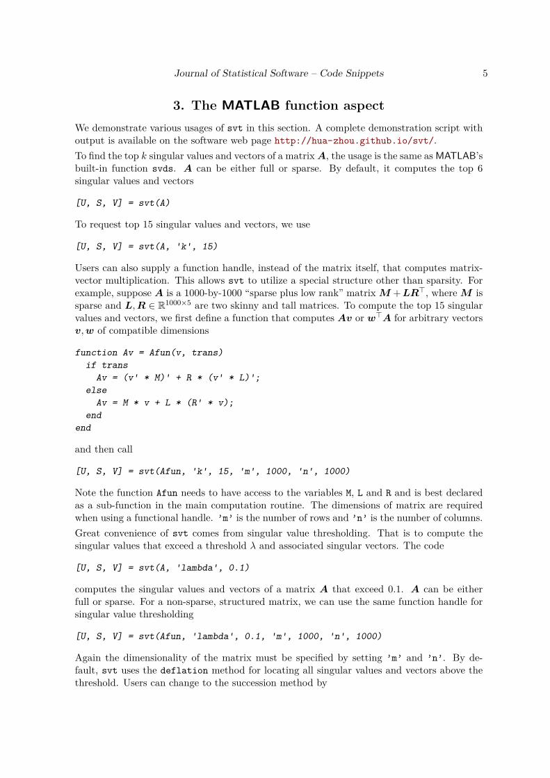
3. The MATLAB function aspectWe demonstrate various usages of svt in this section. A complete demonstration script withoutput is available on the software web page http://hua-zhou.github.io/svt/.To find the top k singular values and vectors of a matrixA, the usage is the same as MATLAB’sbuilt-in function svds. A can be either full or sparse. By default, it computes the top 6singular values and vectors

[U, S, V] = svt(A)

To request top 15 singular values and vectors, we use

[U, S, V] = svt(A, 'k', 15)

Users can also supply a function handle, instead of the matrix itself, that computes matrix-vector multiplication. This allows svt to utilize a special structure other than sparsity. Forexample, suppose A is a 1000-by-1000 “sparse plus low rank” matrix M +LR>, where M issparse and L,R ∈ R1000×5 are two skinny and tall matrices. To compute the top 15 singularvalues and vectors, we first define a function that computes Av or w>A for arbitrary vectorsv,w of compatible dimensions

function Av = Afun(v, trans)if trans

Av = (v' * M)' + R * (v' * L)';else

Av = M * v + L * (R' * v);end

end

and then call

[U, S, V] = svt(Afun, 'k', 15, 'm', 1000, 'n', 1000)

Note the function Afun needs to have access to the variables M, L and R and is best declaredas a sub-function in the main computation routine. The dimensions of matrix are requiredwhen using a functional handle. ’m’ is the number of rows and ’n’ is the number of columns.Great convenience of svt comes from singular value thresholding. That is to compute thesingular values that exceed a threshold λ and associated singular vectors. The code

[U, S, V] = svt(A, 'lambda', 0.1)

computes the singular values and vectors of a matrix A that exceed 0.1. A can be eitherfull or sparse. For a non-sparse, structured matrix, we can use the same function handle forsingular value thresholding

[U, S, V] = svt(Afun, 'lambda', 0.1, 'm', 1000, 'n', 1000)

Again the dimensionality of the matrix must be specified by setting ’m’ and ’n’. By de-fault, svt uses the deflation method for locating all singular values and vectors above thethreshold. Users can change to the succession method by

6 svt: Singular Value Thresholding in MATLAB

[U, S, V] = svt(A, 'lambda', 0.1, 'method', 'succession')

or

[U, S, V] = svt(Afun, 'lambda', 0.1, 'm', 1000, 'n', 1000, 'method', ...'succession')

For singular value thresholding, users can specify the number of top singular values to tryin the first iteration and then increment the size in subsequent iterations by the ’k’ and’incre’ options respectively. The command

[U, S, V] = svt(A, 'lambda', 0.1, 'k', 15, 'incre', 3)

computes the top 15 singular values and vectors in the first iteration and then adds 3 more ineach subsequent iteration until hitting the singular values below threshold 0.1. This optionis useful when users have a rough idea how many singular values are above the threshold andcan save considerable computation time. The default values are k = 6 and incre = 5.

4. Numerical experimentsIn this section, we evaluate the numerical performance of svt in different scenarios and com-pare it with the MATLAB built-in functions svd and svds. We conduct these experimentson a desktop with an Intel Quad Core CPU @ 3.20 GHz and 12 GB of RAM. Computingenvironment is Linux MATLAB R2013a 64-bit version. For testing purpose, we use 5 squaresparse matrices and 4 rectangular sparse matrices of varying sizes downloaded from the Uni-versity of Florida sparse matrix collection (Davis and Hu 2011). For each numerical task,10 replicate runs are performed and the average run time and standard error are reported,unless stated otherwise. Sparsity of a matrix A is defined as the proportion of zero entries, 1- nnz(A)/numel(A).

4.1. Top k singular values and vectors of sparse matrices

Table 1 reports the run times of svt, svds and svd for computing the top 6 singular valuesand associated vectors of sparse matrices. In this case, svt internally calls svds thus theirrun times should be indistinguishable. The huge gain of svt/svds in large sparse matricessimply demonstrates the advantage of the iterative method over the full decomposition methodimplemented in svd.

4.2. Top k singular values and vectors of “sparse + low rank” matrices

This example tests the capability of svt to take functional handle input. We generate struc-tured matrices by adding a low rank perturbation to a sparse matrix. Let M ∈ Rn×nbe a sparse test matrix. We form a “sparse + low rank” matrix A = M + LR>, whereL,R ∈ Rn×10 have independent standard normal distributed entries. Table 2 shows the av-erage run times of svt with function handle input and svds with input A itself to computethe top 6 singular values and vectors based on 10 simulation replicates. It clearly shows theadvantage of exploiting the special matrix structure over applying the iterative algorithm tothe full matrix directly. The speed-up is up to 100 fold for large matrices.

Journal of Statistical Software – Code Snippets 7

Matrix Size Sparsity svt svds svdbfwb398 398 0.9816 0.0396 (0.0003) 0.0393 (0.0004) 0.0450 (0.0001)rdb800l 800 0.9928 0.0944 (0.0008) 0.0941 (0.0009) 0.2184 (0.0007)tols1090 1090 0.9970 0.0549 (0.0007) 0.0592 (0.0005) 0.4377 (0.0006)mhd4800b 4800 0.9988 0.0579 (0.0029) 0.0536 (0.0026) 249.1995 (0.0143)cryg10000 10000 0.9995 0.1550 (0.0019) 0.1580 (0.0017) 1773.6812 (0.2014)

Table 1: Top 6 singular values and vectors of sparse matrices by svt, svds and svd. Reportedare the average run time (in seconds) and standard error (in parentheses) based on 10 runs.

Matrix Size Sparsity svt (fh input) svdsbfwb398 398 0.9816 0.0176 (0.0011) 0.0408 (0.0009)rdb800l 800 0.9928 0.0240 (0.0005) 0.2115 (0.0014)tols1090 1090 0.9970 0.0780 (0.0009) 0.9396 (0.0079)mhd4800b 4800 0.9988 0.0471 (0.0001) 5.6700 (0.0166)cryg10000 10000 0.9995 0.1909 (0.0022) 44.2213 (0.4373)

Table 2: Top 6 singular values and vectors of “sparse + low rank” matrices by svt and svds.Structured matrices are formed by adding a random rank-10 matrix to the original sparse testmatrix. Reported are the average run time (in seconds) and standard error (in parentheses)based on 10 simulation replicates.

Matrix Size Sparsity svt svdbfwb398 398 0.9816 0.3633 (0.0012) 0.0456 (0.0001)rdb800l 800 0.9928 0.7716 (0.0047) 0.2237 (0.0005)tols1090 1090 0.9970 0.4295 (0.0012) 0.4451 (0.0011)mhd4800b 4800 0.9988 1.3733 (0.0075) 249.4558 (0.0423)cryg10000 10000 0.9995 3.1157 (0.0152) 1773.0692 (0.3403)

Table 3: Singular value thresholding of sparse matrices by svt and svd. Reported are theaverage run time (in seconds) and standard error (in parentheses) based on 10 runs. Thethreshold value is pre-determined to catch the top 50 singular values.

4.3. Singular value thresholding of sparse matrices

In this example we compare the singular value thresholding capability of svt with the strategyof full singular value decomposition by svd followed by thresholding on sparse test matrices.The threshold value is pre-determined such that the top 50 singular values are above threshold.By default, svt starts with k = 6 singular values and then add more than 5 in each subsequentiteration. Results are presented in Table 3. For matrices of size less than 1000, svt is lessefficient due to the overhead of repeated calling iterative algorithms until hitting the threshold.For large matrices, svt shows 100 ∼ 1000 fold speed-ups.

4.4. Singular value thresholding of “sparse + low rank” matrices

This example investigates singular value thresholding of structured matrices. “Sparse + lowrank” matrices are generated by the same mechanism as in Section 4.2. Results in Table 4show roughly the same pattern as in Table 3. Speed-up of svt is most eminent for large

8 svt: Singular Value Thresholding in MATLAB

Matrix Size Sparsity svt (fh input) svt (matrix input) svdbfwb398 398 0.9816 1.3540 (0.1486) 1.4209 (0.1744) 0.0502 (0.0002)rdb800l 800 0.9928 2.4144 (0.0089) 2.8655 (0.0194) 0.2569 (0.0005)tols1090 1090 0.9970 0.5100 (0.0023) 1.3044 (0.0051) 0.4455 (0.0005)mhd4800b 4800 0.9988 5.6852 (0.1462) 89.9854 (3.3959) 48.9117 (0.0122)cryg10000 10000 0.9995 3.5793 (0.0145) 104.0540 (0.2411) 443.3518 (0.1034)

Table 4: Singular value thresholding of “sparse + low rank” matrices. Reported are theaverage run time (in seconds) and standard error (in parentheses) based on 10 simulationreplicates. Structured matrices are formed by adding a random rank-10 matrix to the originalsparse test matrix. The threshold value is pre-determined to catch the top 50 singular values.

Matrix Size Sparsity Deflation Successionbfwb398 398 0.9816 0.3626 (0.0012) 0.4055 (0.0026)rdb800l 800 0.9928 0.7636 (0.0048) 0.8670 (0.0019)tols1090 1090 0.9970 0.4250 (0.0016) 0.5167 (0.0013)mhd4800b 4800 0.9988 1.3761 (0.0110) 2.3382 (0.0227)cryg10000 10000 0.9995 3.1782 (0.0173) 5.8789 (0.0648)

Table 5: Comparison of deflation and succession methods for singular value thresholdingof sparse matrices. Reported are the average run time (in seconds) and standard error (inparentheses) based on 10 runs. The threshold is pre-determined to catch the top 50 singularvalues.

matrices. To evaluate the effectiveness of exploiting structure in singular value thresholding,we also call svt with input A directly, which apparently compromises efficiency.

4.5. Deflation versus succession method for singular value thresholding

Table 5 compares the efficiency of the deflation and succession strategies for singular valuethresholding of sparse test matrices. The threshold value is pre-determined such that the top50 singular values are above the threshold. Both methods start with k = 6 singular valuesand then add 5 more in each subsequent iteration. The deflation method is in general fasterthan the succession method.A similar comparison is done on “sparse + low rank” structured matrices, which are generatedin the same way as in Section 4.2. The threshold is again set at the 50th singular value of eachmatrix. The average run time and standard error are reported in Table 6. We found non-convergence of the underlying ARPACK routine when applying the deflation method to therdb800l and mhd4800 matrices. The non-convergence is caused by clustered eigenvalues. It iswell known that ARPACK works best for finding eigenvalues with large separation betweenunwanted ones, and non-convergence is typical when dealing with ill conditioned matrices(Lehoucq and Sorensen 1996). When this happens, we restart with the succession methodand continue from the current subspace.

4.6. Large-scale singular value thresholding

The purpose of this section is to demonstrate the performance of svt on large rectangularmatrices. For the first two test matrices (bibd_20_10 and bibd_22_8), “sparse + low rank”

Journal of Statistical Software – Code Snippets 9

Matrix Size Sparsity Deflation Successionbfwb398 398 0.9816 1.2936 (0.0588) 2.0956 (0.0059)rdb800l 800 0.9928 2.3758 (0.0187) 1.3863 (0.0118)tols1090 1090 0.9970 0.5084 (0.0022) 0.6088 (0.0011)mhd4800b 4800 0.9988 5.6008 (0.1598) 4.4027 (0.0396)cryg10000 10000 0.9995 3.5636 (0.0129) 6.3697 (0.0621)

Table 6: Comparison of deflation and succession methods for singular value thresholding of“sparse + low rank” matrices. Reported are the average run time (in seconds) and standarderror (in parentheses) based on 10 simulation replicates. The threshold is pre-determined tocatch the top 50 singular values.

Matrix Size Sparsity 5th 20th 50thbibd_20_10 (190, 184756) 0.7632 0.0350 0.6152 11.2083bibd_22_8 (231, 319770) 0.8788 0.0372 2.6438 4.1058

stormG2_1000 (528185, 1377306) 0.9999 0.2518 1.0394 12.6890tp-6 (142752, 1014301) 0.9999 1.6373 20.2409 41.3021

Table 7: Singular value thresholding of large rectangular matrices. Reported are the run time(in minutes) of svt from one replicate. The threshold value is pre-determined to catch thetop 5, 20, and 50 singular values respectively.

matrices are generated by the same mechanism as in Section 4.2. For the other two matrices(sotrmG2_1000 and tp-6), singular value thresholding is performed on the original sparsematrices. The threshold is set at the 5th, 20th, and 50th singular value of each matrixrespectively. Table 7 displays the run time of svt from one replicate. The full singular valuedecomposition svd takes excessively long time for these 4 problems so its results are notreported.

4.7. Application to matrix completion problem

To demonstrate the effectiveness of svt as a plug-in computational routine in practice, we con-duct a numerical experiment on the spectral regularization algorithm for matrix completion(Mazumder et al. 2010), which minimizes

12∑

(i,j)∈Ω(xij − yij)2 + λ‖X‖∗ (4)

at a grid of tuning parameter values λ. Here Ω indexes the observed entries yij and X = (xij)is the completed matrix. Algorithm 3 lists the computational algorithm, which involvesrepeated singular value thresholding (lines 4–6). See Chi et al. (2013) for a derivation fromthe majorization-minimization (MM) point of view. Although A(t) is is a dense matrix, itcan be written as

A(t) = PΩ(Y ) + PΩ⊥(X(t))= [PΩ(Y )− PΩ(X(t))] + X(t),

where X(t) is a low rank matrix at large values of λ (only few singular values survive afterthresholding), and PΩ(·) is a binary projection operator onto the observed entries. Fortu-

10 svt: Singular Value Thresholding in MATLAB

Algorithm 3: MM algorithm for minimizing the penalized loss (4).1 Initialize X(0) ;2 repeat3 A(t) ← PΩ(Y ) + PΩ⊥(X(t)) ;4 SVD Udiag(a(t))V > ← A(t) ;5 x(t+1) ← (a(t) − λ)+ ;6 X(t+1) ← Udiag(x(t+1))V > ;7 until objective value converges;

Size Sparsity Rank Grid points svt (fh input) svt (matrix input) svd500 0.95 5 15 0.8541 0.7335 0.5466

1000 0.95 5 19 2.9359 4.0803 4.27632000 0.95 5 20 10.3611 35.7058 40.15623000 0.95 5 20 20.6781 69.3164 138.80114000 0.95 5 20 52.2150 175.2524 335.23735000 0.95 5 20 71.8051 246.3738 630.2729

Table 8: Run time of matrix completion problem using different singular value thresholdingmethods. Reported are the run time (in minutes) for the whole solution path. Path followingis terminated whenever 20 grid points are exhausted or the rank of solution goes beyond 10(twice the true rank).

nately, in many applications, large values of λ are the regime of interest, which encourageslow rank solutions. That means most of the time A(t) is of the special form “sparse + lowrank” that enables extremely fast matrix-vector multiplication.In the numerical experiment, we generate a rank-5 matrix by multiplying two matrices M =LR>, where L,R ∈ Rn×5 have independent standard normal distributed entries. Then, weadd independent standard Gaussian noise to corrupt the original parameter matrix M , thatis Y = M + ε. 5% entries of Y are randomly chosen to be observed. The dimension n of oursynthetic data ranges from 500 to 5000. For each n, we minimize (4) at a grid of 20 points.The grid is set up in a linear manner as in Mazumder et al. (2010).

lambdas = linspace(maxlambda * 0.9, maxlambda / 5, 20)

Here maxlambda is the largest singular value of the input matrix Y with missing entries setat 0. Warm start strategy is used. That is the solution at a previous λ is used as the startpoint for the next λ. Path following is terminated whenever all 20 grid points are exhaustedor the rank of the solution exceeds 10 (twice the true rank). Three methods for singular valuethresholding are tested: svt using functional handle input, svt using matrix input A(t), andfull singular value thresholding by svd followed by thresholding. Table 8 shows the run timein minutes for obtaining the whole solution path. Speed-up of svt increases with matrix sizeand utilizing the “sparse + low rank” structure via functional handle boosts the performance.

Journal of Statistical Software – Code Snippets 11

5. DiscussionWe develop a MATLAB wrapper function svt for singular value thresholding. When a fixednumber of top singular values and vectors are requested, svt expands the capability ofMATLAB’s built-in function svds by allowing function handle input. This enables appli-cation of the iterative method to dense but structured large matrices. More conveniently,svt provides a simple interface for singular value thresholding, the key step in many ma-trix learning algorithms. Our numerical examples have demonstrated efficiency of svt invarious situations. The svt package is continuously developed and maintained at GitHubhttp://hua-zhou.github.io/svt/.We describe a few future directions here. Our wrapper function utilizes the well-knownrelationship between SVD and eigen-decomposition of the augmented matrix (3) and buildson the MATLAB’s eigs function, which in turn calls the ARPACK subroutines (Lehoucq,Sorensen, and Yang 1997) for solving large scale eigenproblems. An alternative is to usethe PROPACK library (Larsen 1998), an efficient package for singular value decompositionof sparse or structured matrices. This involves distributing extra source code or compiledprograms but may further improve efficiency. Both ARPACK and PROPACK implementKrylov subspace method and compute a fixed number of top eigenvalues or singular values.Thus singular value thresholding has to be done in a sequential manner. The recent FEASTpackage (Plizzi and Kestyn 2012) is an innovative method for solving standard or generalizedeigenvalue problems, and is able to compute all the eigenvalues and eigenvectors within agiven search interval, which is particularly attractive for the singular value thresholding task.However users must provide an initial value for the number of eigenvalues in the searchinterval. If the initial guess is too small, the program will exit. In real applications of singularvalue thresholding, such an estimate may be hard to obtain. Further investigation of thefeasibility of using FEAST for singular value thresholding is underway.

AcknowledgmentsThe work is partially supported by NSF grant DMS-1310319 and NIH grants HG006139,GM105785, and GM53275.

References

ACM SIGKDD, Netflix (2007). “Proceedings of KDD Cup and Workshop.” In Proceedings ofKDD Cup and Workshop. URL http://www.cs.uic.edu/liub/Netflix-KDD-Cup-2007.html.

Boyd S, Parikh N, Chu E, Peleato B, Eckstein J (2011). “Distributed Optimization andStatistical Learning via the Alternating Direction Method of Multipliers.” Foundations andTrends® in Machine Learning, 3(1), 1–122. doi:10.1561/2200000016.

Cai JF, Candès EJ, Shen Z (2010). “A Singular Value Thresholding Algorithm for MatrixCompletion.” SIAM Journal on Optimization, 20(4), 1956–1982. doi:10.1137/080738970.

Candès EJ, Recht B (2009). “Exact Matrix Completion via Convex Optimization.” Founda-tions of Computational Mathematics, 9(6), 717–772. doi:10.1007/s10208-009-9045-5.

12 svt: Singular Value Thresholding in MATLAB

Chi EC, Zhou H, Chen GK, Del Vecchyo DO, Lange K (2013). “Genotype Imputation viaMatrix Completion.” Genome Research, 23(3), 509–518. doi:10.1101/gr.145821.112.

Davis TA, Hu Y (2011). “The University of Florida Sparse Matrix Collection.” ACM Trans-actions on Mathematical Software, 38(1), Article No. 1. doi:10.1145/2049662.2049663.

Goldstein T, Studer C, Baraniuk R (2015). “FASTA: A Generalized Implementation ofForward-Backward Splitting.” arXiv:1501.04979 [cs.MS], URL http://arxiv.org/abs/1501.04979.

Golub GH, Van Loan CF (1996). Matrix Computations. Johns Hopkins Studies in theMathematical Sciences, 3rd edition. Johns Hopkins University Press, Baltimore.

Kalofolias V, Bresson X, Bronstein MM, Vandergheynst P (2014). “Matrix Completion onGraphs.” CoRR, abs/1408.1717. URL http://infoscience.epfl.ch/record/203064/files/kalofolias_2014.pdf.

Lange K, Chi EC, Zhou H (2014). “A Brief Survey of Modern Optimization for Statisticians.”International Statistical Review, 82(1), 46–70. doi:10.1111/insr.12022.

Larsen RM (1998). “Lanczos Bidiagonalization with Partial Reorthogonalization.” Technicalreport DAIMI PB-357, Department of Computer Science, Aarhus University.

Lehoucq RB, Sorensen DC (1996). “Deflation Techniques for an Implicitly Restarted ArnoldiIteration.” SIAM Journal on Matrix Analysis and Applications, 17(4), 789–821. doi:10.1137/s0895479895281484.

Lehoucq RB, Sorensen DC, Yang C (1997). “ARPACK Users Guide: Solution of Large ScaleEigenvalue Problems by Implicitly Restarted Arnoldi Methods.”

Mazumder R, Hastie T, Tibshirani R (2010). “Spectral Regularization Algorithms for Learn-ing Large Incomplete Matrices.” Journal of Machine Learning Research, 11, 2287–2322.

Otazo R, Candès E, Sodickson DK (2015). “Low-Rank Plus Sparse Matrix Decompositionfor Accelerated Dynamic MRI with Separation of Background and Dynamic Components.”Magnetic Resonance in Medicine, 73, 1125–1136.

Parikh N, Boyd S (2013). “Proximal Algorithms.” Foundations and Trends in MachineLearning, 1(3), 123–231. doi:10.1561/2200000016.

Plizzi E, Kestyn J (2012). “FEAST Eigenvalue Solver v3.0 User Guide.” arXiv:1203.4031[cs.MS], URL http://arxiv.org/abs/1203.4031.

The MathWorks Inc (2013). MATLAB – The Language of Technical Computing, VersionR2013a. Natick. URL http://www.mathworks.com/products/matlab/.

Yang C, Wang L, Zhang S, Zhao H (2013). “Accounting for Non-Genetic Factors by Low-Rank Representation and Sparse Regression for eQTL Mapping.” Bioinformatics, 29(8),1026–1034.

Yuan M, Ekici A, Lu Z, Monteiro R (2007). “Dimension Reduction and Coefficient Estimationin Multivariate Linear Regression.” Journal of the Royal Statistical Society B, 69(3), 329–346.

Journal of Statistical Software – Code Snippets 13

Zhang Y, Zhou H, Zhou J, Sun W (2017). “Regression Models for Multivariate Count Data.”Journal of Computational and Graphical Statistics, 26(1), 1–13. doi:10.1080/10618600.2016.1154063.

Zhou H, Li L (2014). “Regularized Matrix Regressions.” Journal of Royal Statistical SocietyB, 76(2), 463–483.

Zhou X, Liu J, Wan X, Yu W (2014). “Piecewise-Constant and Low-Rank Approximation forIdentification of Recurrent Copy Number Variations.” Bioinformatics, 30(14), 1943–1949.doi:10.1093/bioinformatics/btu131.

Affiliation:Cai LiDepartment of StatisticsNorth Carolina State University2311 Stinson DriveRaleigh, NC 27695-8203, United States of AmericaE-mail: cli9@ncsu.eduURL: http://www4.ncsu.edu/~cli9/

Hua ZhouDepartment of BiostatisticsUniversity of California, Los AngelesBox 951772, 21-254A CHSLos Angeles, CA 90095-1772, United States of AmericaTelephone: +1/310/794-7835E-mail: huazhou@ucla.eduURL: http://hua-zhou.github.io/

Journal of Statistical Software http://www.jstatsoft.org/published by the Foundation for Open Access Statistics http://www.foastat.org/

November 2017, Volume 81, Code Snippet 2 Submitted: 2014-08-04doi:10.18637/jss.v081.c02 Accepted: 2016-09-09