SUZANNE CHILDRESS, ERIK SABINA, DAVID KURTH, TOM ROSSI , JENNIFER MALM

DRCOG Focus Activity-Based Model Calibration/Validation

Innovations in Travel Modeling ConferenceMay 12, 2010

Focus Model Flow

Population Synthesizer

Highway and Transit

Skimming

Regular Workplace Location

Regular School Location

Auto Availability

Daily Activity Pattern/Exact

Number of Tours

Tour Primary Destination

Choice

Tour Mode Choice

Tour Time of Day Choice

Intermediate Stop

Generation

Intermediate Stop Location

Trip Mode Choice

Trip Time of Day

Highway and Transit

Assignment

(Simplified)

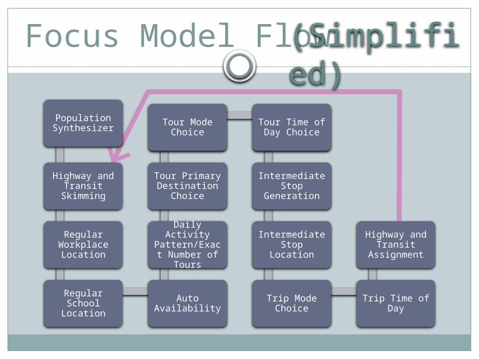
Model Estimation Data: 1997 Travel Behavior Inventory (TBI)

Next Steps:1997 Validation

Calibrated to 2005 2035 Forecast

Extensive Model Calibration/Validation Plan

What’s the plan?

Data Sources

1997 TBI

2000 CTPP

Other 2000

Census

2005 ACS

2005 State

Demo-grapher

2005 Traffic/ Transit Counts

2005 HPMS VMT

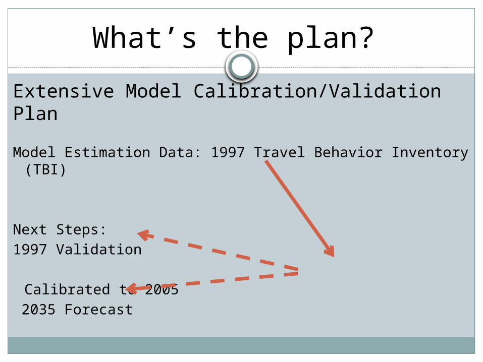
Location Data At Point Level

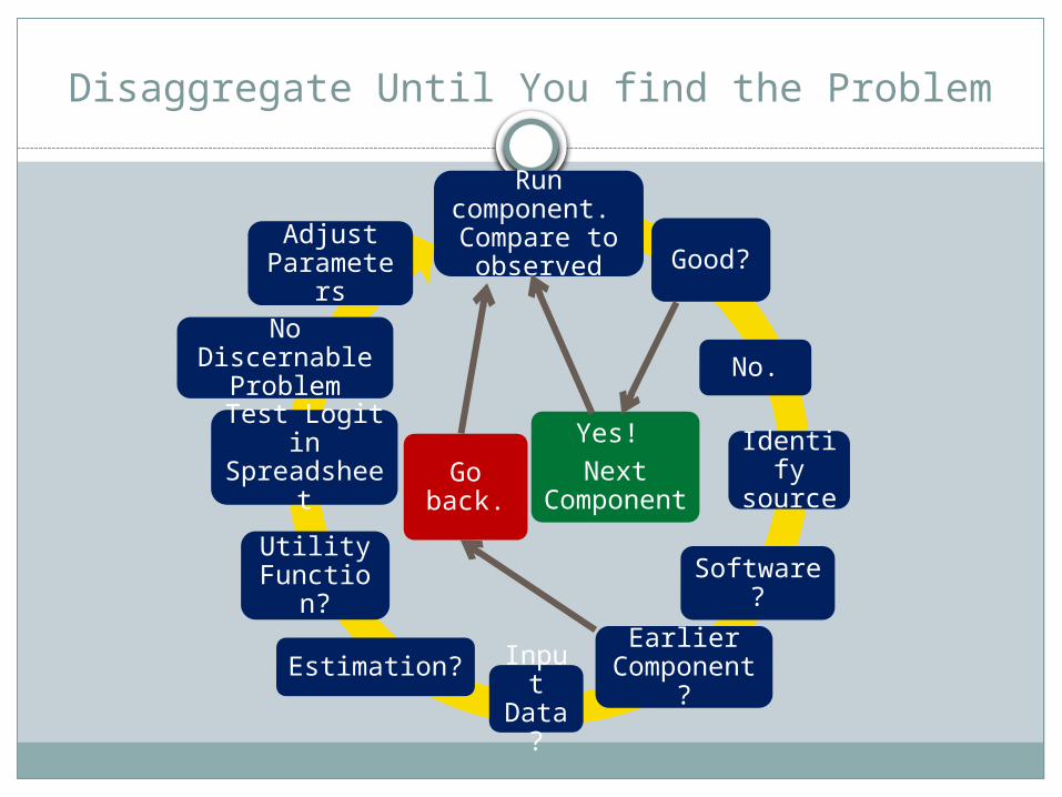
Run component. Compare to

observed Good?

No.

Identify source

Software?

Earlier Component

?Input Data?

Estimation?

Utility Function

?

Test Logit in Spreadsheet

No Discernable

Problem

Adjust Parameter

s

Disaggregate Until You find the Problem

Yes! Next

Component

Go back.

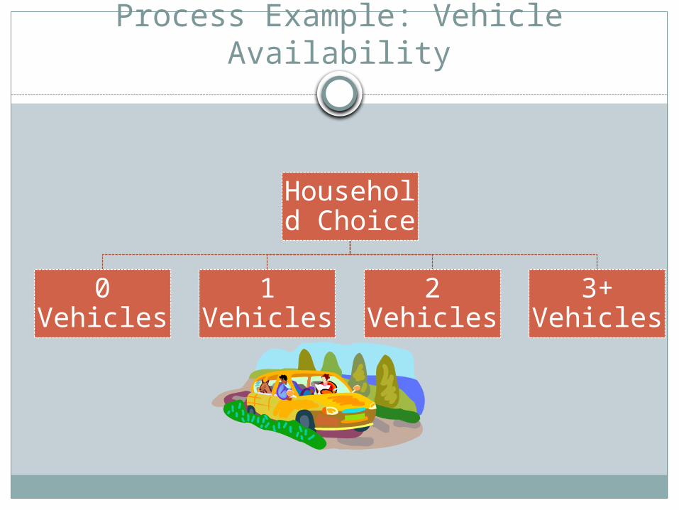
Process Example: Vehicle Availability

Household Choice

0 Vehicles

1 Vehicles

2 Vehicles

3+ Vehicles

Utility Function Example (simplified)

 Utility (No Vehicle) = -5.603 * 1 HH Driver-6.598 * 2 HH Drivers-6.598 * 3 HH Drivers-6.598 * 4+ HH Drivers+0.729 * (Cars >= Workers?)++...

+3.735 * (HH income < $15k/year?)+1.408 * (HH income between $15k/year - $30k/year?)-1.412 * (HH income between $75k/year - $100k/year?)-1.641 * (HH income > $100k/year)+6.211 * Transit Accessibility

Vehicle Availability - NO Calibration

Household Vehicles

2005 Model

2005 ACS

2000 Census

0 vehicles 4% 7% 6%1 vehicles 30% 33% 33%2 vehicles 42% 40% 41%3+ vehicles 25% 19% 20%

Regional Households by Number of Vehicles:

Disaggregate–Where is Problem the Worst?

Household Vehicles Adams Arapahoe Boulder Denver Douglas Jefferson

0 vehicles 3% 3% 3% 6% 1% 2%

1 vehicle 26% 29% 29% 39% 17% 27%

2 vehicles 42% 42% 43% 35% 53% 44%

3+ vehicles 28% 25% 25% 20% 29% 27%

Household Vehicles Adams Arapahoe Boulder Denver Douglas Jefferson

0 vehicles 4% 5% 4% 12% 1% 4%

1 vehicle 32% 34% 29% 43% 20% 32%

2 vehicles 41% 41% 46% 33% 55% 41%

3+ vehicles 23% 20% 21% 12% 24% 23%

2005 Model: Households by County by Vehicle Availability

2005 ACS: Households by County by Vehicle Availability

Set Up Logit Model in a Spreadsheet (simplified)

ALTERNATIVE No Car  1 Car 2 Car  3 Car 4+ Car

Variable Name Coeff Term Coeff Term Coeff Term Coeff Term Coeff Term1 driver in HH -5.6 -5.6     -1.8 -1.8 -3.4 -3.4 -4.2 -4.22 drivers in HH -6.6 0.0 -2.6 0.0     -1.4 0.0 -2.6 0.03 drivers in HH -6.6 0.0 -2.7 0.0 -1.5 0.0     -1.1 0.04+ drivers in HH -6.6 0.0 -2.2 0.0 -2.1 0.0 -1.4 0.0    HH inc under $15k/yr 3.7 3.7 1.1 1.1     -0.2 -0.2 -1.5 -1.5HH inc $15k-30k/yr 1.4 0.0 0.4 0.0     -0.2 0.0 -0.2 0.0HH inc $75k-100k/yr -1.4 0.0 -0.7 0.0     0.2 0.0 0.4 0.0HH inc above $100k/yr -1.6 0.0 -1.6 0.0     0.3 0.0 0.5 0.0Transit Accessibilitiy 6.2 0.0 1.3 0.0 1.3 0.0 1.3 0.0 1.3 0.0                                          UTILITY   -1.1   1.8   -1.0   -2.9   -5.0EXP(Utility)   0.3   6.2   0.4   0.1   0.0Sum of EXP(Utility)   6.9   6.9   6.9   6.9   6.9

Probability 4.6% 

89.3% 

5.1% 

0.8% 

0.1%

Get Your Software to Write Out All Coefficients, Variable Values, and Utilities

2010-02-11 16:08:37,098 DEBUG 5268 IRMCommon.UtilityFunctionTerm - Constant Value is -4.86

2010-02-11 16:08:37,098 DEBUG 5268 IRMCommon.UtilityFunction - Running Utility Sum is -4.86

2010-02-11 16:08:37,098 DEBUG 5268 IRMCommon.UtilityFunctionTerm - Coefficient is 1.18, Variable Name is PersTypeUniversity, Variable Value is 1.

2010-02-11 16:08:37,098 DEBUG 5268 IRMCommon.UtilityFunction - Running Utility Sum is -3.68

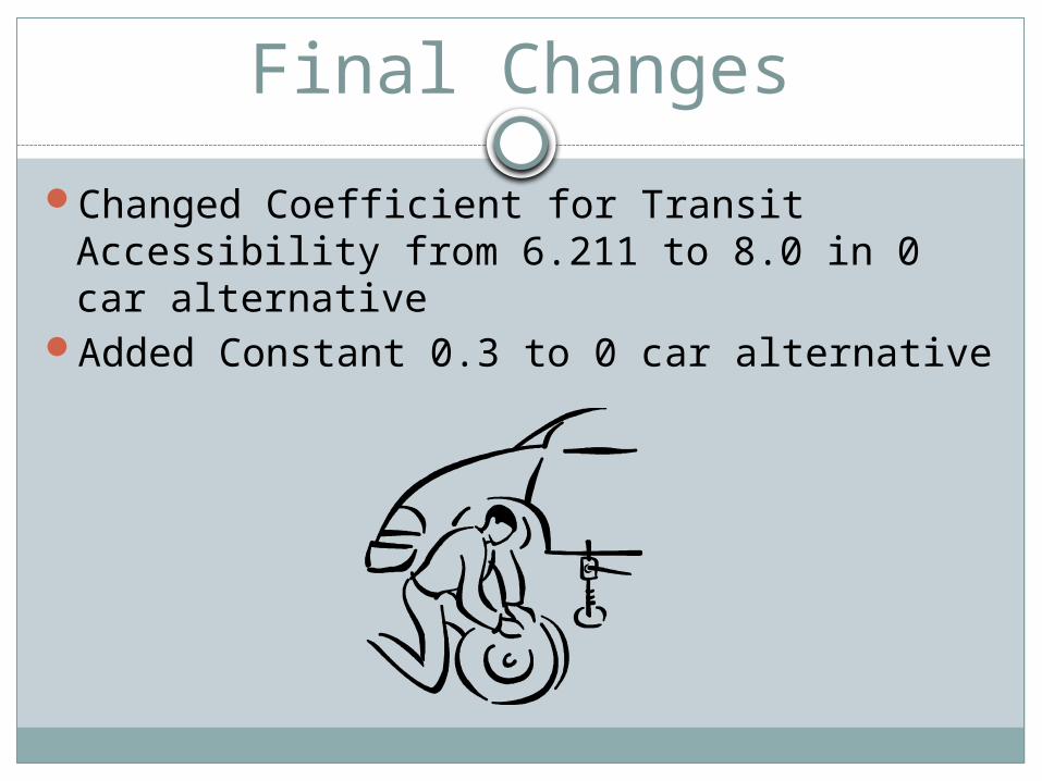
Final Changes

Changed Coefficient for Transit Accessibility from 6.211 to 8.0 in 0 car alternative

Added Constant 0.3 to 0 car alternative

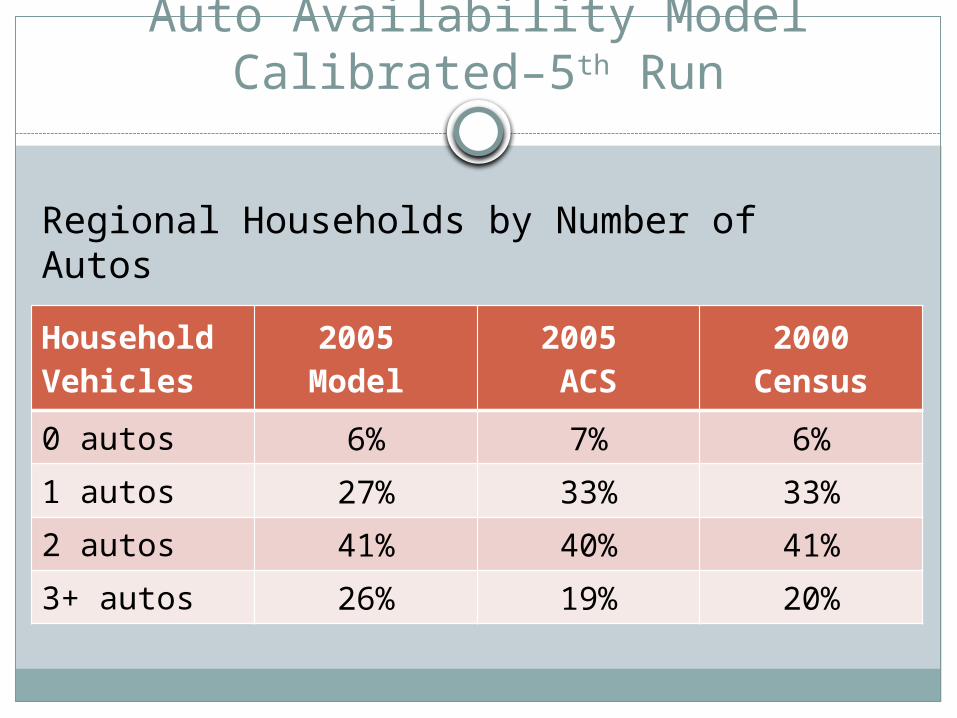
Auto Availability Model Calibrated–5th Run

Household Vehicles

2005 Model

2005 ACS

2000 Census

0 autos 6% 7% 6%

1 autos 27% 33% 33%

2 autos 41% 40% 41%

3+ autos 26% 19% 20%

Regional Households by Number of Autos

Auto Availability Model Calibrated–5th Run

Household Vehicles Adams Arapahoe Boulder Denver Douglas Jefferson

0 vehicles 6% 7% 5% 9% 2% 4%

1 vehicle 25% 22% 27% 36% 16% 26%

2 vehicles 42% 38% 46% 35% 53% 44%

3+ vehicles 28% 33% 22% 20% 29% 26%

Household Vehicles Adams Arapahoe Boulder Denver Douglas Jefferson

0 vehicles 4% 5% 4% 12% 1% 4%

1 vehicle 32% 34% 29% 43% 20% 32%

2 vehicles 41% 41% 46% 33% 55% 41%

3+ vehicles 23% 20% 21% 12% 24% 23%

2005 Model: Households by County by Vehicle Availability

2005 ACS: Households by County by Vehicle Availability

Final Thoughts

Make a plan – How good does the model have to be? By when? For what purpose?

Be creative in comparison – For data sources and summaries. Look at as much as possible.

Break the problem down until the source is revealed.

Do an alternate year run – May reveal other issues with calibration. Important for validation.

Person Trips By Mode

Bike

Drive

Alone

Drive

to T

rans

it

Scho

olBus

Shar

ed R

ide

2

Shar

ed R

ide

3+W

alk

Wal

k to

Tra

nsit

0%5%

10%15%20%25%30%35%40%45%50%

Ob-served

Average Tours per Person per Day By Tour Purpose

0.00

0.05

0.10

0.15

0.20

0.25

0.30

0.35

0.40

0.45

0.50Modeled

Observed

Trips By Time of Day

4:00

AM

5:00

AM

6:00

AM

7:00

AM

8:00

AM

9:00

AM

10:0

0 AM

11:0

0 AM

12:0

0 PM

1:00

PM

2:00

PM

3:00

PM

4:00

PM

5:00

PM

6:00

PM

7:00

PM

8:00

PM

9:00

PM

10:0

0 PM

11:0

0 PM

12:0

0 AM

1:00

AM

2:00

AM

3:00

AM

0%

1%

2%

3%

4%

5%

6%

7%

8%

9%

10%

TBI Total

IRM_Total

Start of Time Period Hour

% o

f A

ll T

rips

Modeled Versus Observed VMT

# Links With Counts

Modeled VMT With Counts

Actual VMTWith Counts %Error

1,683 21,166,000 20,507,000 3.2%

Total VMT by Facility Type

Facility Type #Links Modeled VMT

% Modeled VMT

ActualVMT

% Actual VMT

Difference of Percents

Freeway 210 8,791,000 42% 9,605,000 47% -8%

Major Regional Arterial 71 1,834,000 9% 1,587,000 8% 16%

Principal Arterial 863 8,990,000 43% 7,452,000 36% 21%

Minor Arterial 316 1,121,000 5% 1,279,000 6% -12%

Collector 218 406,000 2% 558,000 3% -27%

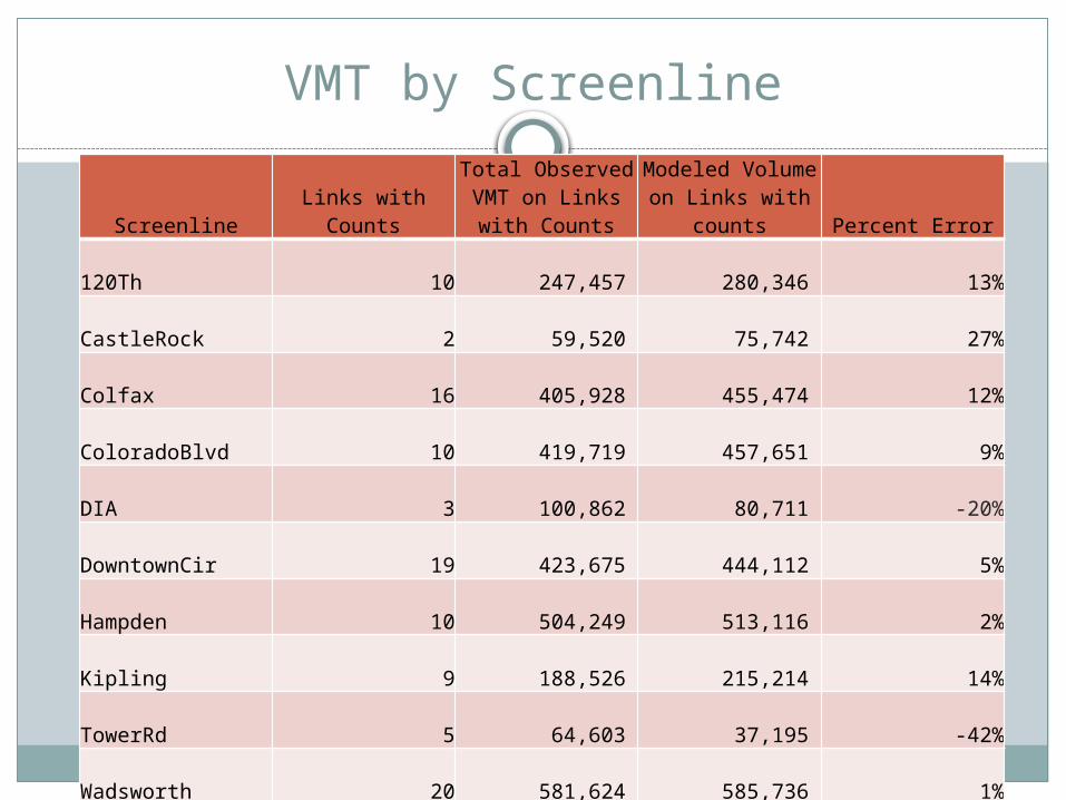
VMT by Screenline

Screenline Links with Counts

Total Observed VMT on Links with

Counts

Modeled Volumeon Links with

counts Percent Error

120Th 10 247,457

280,346 13%

CastleRock 2 59,520

75,742 27%

Colfax 16 405,928

455,474 12%

ColoradoBlvd 10 419,719

457,651 9%

DIA 3 100,862

80,711 -20%

DowntownCir 19 423,675

444,112 5%

Hampden 10 504,249

513,116 2%

Kipling 9 188,526

215,214 14%

TowerRd 5 64,603

37,195 -42%

Wadsworth 20 581,624

585,736 1%

Transit trips by sub-mode

Submode 2005 Observed 2005 Modeled

Difference:Observed-Modeled

Mall Shuttle 47,276 56,606 -9,330

Denver Local 123,821 172,231 -48,410

Denver Limited 17,497 19,943 -2,446

Boulder Local 19,210 21,983 -2,773

Longmont Local 689 2,385 -1,696

Express 10,741 24,737 -13,996

Regional 11,355 9,972 1,383

skyRide 5,121 542 4,579

Light Rail 34,578 44,689 -10,111

Total 270,288 353,088 -82,800