Suspension geometry and computation john c. dixon

Suspension Geometryand Computation

By the same author:

The Shock Absorber Handbook, 2nd edn (Wiley, PEP, SAE)

Tires, Suspension and Handling, 2nd edn (SAE, Arnold).

The High-Performance Two-Stroke Engine (Haynes)

Suspension Geometryand Computation

John C. Dixon, PhD, F.I.Mech.E., F.R.Ae.S.

Senior Lecturer in Engineering Mechanics

The Open University, Great Britain.

This edition first published 2009

� 2009 John Wiley & Sons Ltd

Registered office

John Wiley & Sons Ltd, The Atrium, Southern Gate, Chichester, West Sussex, PO19 8SQ, United Kingdom

For details of our global editorial offices, for customer services and for information about how to apply for permission to

reuse the copyright material in this book please see our website at www.wiley.com.

The right of the author to be identified as the author of this work has been asserted in accordance with the Copyright,

Designs and Patents Act 1988.

All rights reserved. No part of this publication may be reproduced, stored in a retrieval system, or transmitted, in any

form or by any means, electronic, mechanical, photocopying, recording or otherwise, except as permitted by the UK

Copyright, Designs and Patents Act 1988, without the prior permission of the publisher.

Wiley also publishes its books in a variety of electronic formats. Some content that appears in printmay not be available

in electronic books.

Designations used by companies to distinguish their products are often claimed as trademarks. All brand names and

product names used in this book are trade names, servicemarks, trademarks or registered trademarks of their respective

owners. The publisher is not associatedwith any product or vendormentioned in this book. This publication is designed

to provide accurate and authoritative information in regard to the subject matter covered. It is sold on the understanding

that the publisher is not engaged in rendering professional services. If professional advice or other expert assistance is

required, the services of a competent professional should be sought.

Library of Congress Cataloging-in-Publication Data

Dixon, John C., 1948-

Suspension geometry and computation / John C. Dixon.

p. cm.

Includes bibliographical references and index.

ISBN 978-0-470-51021-6 (cloth)

1. Automobiles–Springs and suspension–Mathematics.

2. Automobiles–Steering-gear–Mathematics. 3. Automobiles–Stability. 4. Roads–Mathematical

models. I. Title.

TL257.D59 2009

629.2’43–dc22

2009035872

ISBN: 9780470510216

A catalogue record for this book is available from the British Library.

Typeset in 9/11 pt Times by Thomson Digital, Noida, India.

Printed in Great Britain by Antony Rowe Ltd, Chippenham, Wiltshire.

Disclaimer: This book is not intended as a guide for vehicle modification, and anyonewho uses it as such does so

entirely at their own risk. Testing vehicle performance may be dangerous. The author and publisher are not liable

for consequential damage arising from application of any information in this book.

www.wiley.com

This work is dedicated to

Aythe

the beautiful goddess of truth, hence also of science and mathematics, and of good

computer programs.

Her holy book is the book of nature.

Contents

Preface xv

1 Introduction and History 1

1.1 Introduction 1

1.2 Early Steering History 1

1.3 Leaf-Spring Axles 3

1.4 Transverse Leaf Springs 8

1.5 Early Independent Fronts 10

1.6 Independent Front Suspension 13

1.7 Driven Rigid Axles 20

1.8 De Dion Rigid Axles 24

1.9 Undriven Rigid Axles 24

1.10 Independent Rear Driven 26

1.11 Independent Rear Undriven 32

1.12 Trailing-Twist Axles 34

1.13 Some Unusual Suspensions 35

References 42

2 Road Geometry 43

2.1 Introduction 43

2.2 The Road 45

2.3 Road Curvatures 48

2.4 Pitch Gradient and Curvature 49

2.5 Road Bank Angle 51

2.6 Combined Gradient and Banking 53

2.7 Path Analysis 53

2.8 Particle-Vehicle Analysis 55

2.9 Two-Axle-Vehicle Analysis 57

2.10 Road Cross-Sectional Shape 59

2.11 Road Torsion 61

2.12 Logger Data Analysis 61

References 63

3 Road Profiles 65

3.1 Introduction 65

3.2 Isolated Ramps 65

3.3 Isolated Bumps 67

3.4 Sinusoidal Single Paths 69

3.5 Sinusoidal Roads 71

3.6 Fixed Waveform 74

3.7 Fourier Analysis 75

3.8 Road Wavelengths 77

3.9 Stochastic Roads 77

References 82

4 Ride Geometry 83

4.1 Introduction 83

4.2 Wheel and Tyre Geometry 83

4.3 Suspension Bump 88

4.4 Ride Positions 88

4.5 Pitch 90

4.6 Roll 90

4.7 Ride Height 92

4.8 Time-Domain Ride Analysis 95

4.9 Frequency-Domain Ride Analysis 96

4.10 Workspace 97

5 Vehicle Steering 99

5.1 Introduction 99

5.2 Turning Geometry – Single Track 100

5.3 Ackermann Factor 103

5.4 Turning Geometry – Large Vehicles 108

5.5 Steering Ratio 111

5.6 Steering Systems 112

5.7 Wheel Spin Axis 113

5.8 Wheel Bottom Point 116

5.9 Wheel Steering Axis 118

5.10 Caster Angle 118

5.11 Camber Angle 119

5.12 Kingpin Angle Analysis 120

5.13 Kingpin Axis Steered 123

5.14 Steer Jacking 124

References 125

6 Bump and Roll Steer 127

6.1 Introduction 127

6.2 Wheel Bump Steer 127

6.3 Axle Steer Angles 131

6.4 Roll Steer and Understeer 132

6.5 Axle Linear Bump Steer and Roll Steer 133

6.6 Axle Non-Linear Bump Steer and Roll Steer 134

6.7 Axle Double-Bump Steer 136

6.8 Vehicle Roll Steer 136

6.9 Vehicle Heave Steer 137

viii Contents

6.10 Vehicle Pitch Steer 137

6.11 Static Toe-In and Toe-Out 138

6.12 Rigid Axles with Link Location 138

6.13 Rigid Axles with Leaf Springs 140

6.14 Rigid Axles with Steering 140

References 141

7 Camber and Scrub 143


7.2 Wheel Inclination and Camber 143

7.3 Axle Inclination and Camber 145

7.4 Linear Bump and Roll 147

7.5 Non-Linear Bump and Roll 149

7.6 The Swing Arm 150

7.7 Bump Camber Coefficients 152

7.8 Roll Camber Coefficients 152

7.9 Bump Scrub 153

7.10 Double-Bump Scrub 156

7.11 Roll Scrub 156

7.12 Rigid Axles 156

References 156

8 Roll Centres 157


8.2 The Swing Arm 158

8.3 The Kinematic Roll Centre 160

8.4 The Force Roll Centre 162

8.5 The Geometric Roll Centre 164

8.6 Symmetrical Double Bump 165

8.7 Linear Single Bump 167

8.8 Asymmetrical Double Bump 169

8.9 Roll of a Symmetrical Vehicle 171

8.10 Linear Symmetrical Vehicle Summary 173

8.11 Roll of an Asymmetrical Vehicle 174

8.12 Road Coordinates 175

8.13 GRC and Latac 177

8.14 Experimental Roll Centres 177

References 178

9 Compliance Steer 179


9.2 Wheel Forces and Moments 180

9.3 Compliance Angles 182

9.4 Independent Suspension Compliance 182

9.5 Discussion of Matrix 184

9.6 Independent-Suspension Summary 185

9.7 Hub Centre Forces 186

9.8 Steering 187

Contents ix

9.9 Rigid Axles 187

9.10 Experimental Measurements 188

References 188

10 Pitch Geometry 189


10.2 Acceleration and Braking 189

10.3 Anti-Dive 190

10.4 Anti-Rise 192

10.5 Anti-Lift 192

10.6 Anti-Squat 193

10.7 Design Implications 193

11 Single-Arm Suspensions 195


11.2 Pivot Axis Geometry 196

11.3 Wheel Axis Geometry 200

11.4 The Trailing Arm 201

11.5 The Sloped-Axis Trailing Arm 205

11.6 The Semi-Trailing Arm 207

11.7 The Low-Pivot Semi-Trailing Arm 209

11.8 The Transverse Arm 210

11.9 The Sloped-Axis Transverse Arm 212

11.10 The Semi-Transverse Arm 214

11.11 The Low-Pivot Semi-Transverse Arm 216

11.12 General Case Numerical Solution 216

11.13 Comparison of Solutions 218

11.14 The Steered Single Arm 222

11.15 Bump Scrub 223

References 226

12 Double-Arm Suspensions 227


12.2 Configurations 228

12.3 Arm Lengths and Angles 229

12.4 Equal Arm Length 230

12.5 Equally-Angled Arms 230

12.6 Converging Arms 231

12.7 Arm Length Difference 232

12.8 General Solution 233

12.9 Design Process 236

12.10 Numerical Solution in Two Dimensions 237

12.11 Pitch 239

12.12 Numerical Solution in Three Dimensions 242

12.13 Steering 243

12.14 Strut Analysis in Two Dimensions 244

12.15 Strut Numerical Solution in Two Dimensions 247

12.16 Strut Design Process 248

12.17 Strut Numerical Solution in Three Dimensions 249

x Contents

12.18 Double Trailing Arms 250

12.19 Five-Link Suspension 251

13 Rigid Axles 253


13.2 Example Configuration 253

13.3 Axle Variables 253

13.4 Pivot-Point Analysis 257

13.5 Link Analysis 258

13.6 Equivalent Links 260

13.7 Numerical Solution 260

13.8 The Sensitivity Matrix 263

13.9 Results: Axle 1 264

13.10 Results: Axle 2 265

13.11 Coefficients 266

14 Installation Ratios 271


14.2 Motion Ratio 271

14.3 Displacement Method 274

14.4 Velocity Diagrams 274

14.5 Computer Evaluation 275

14.6 Mechanical Displacement 275

14.7 The Rocker 276

14.8 The Rigid Arm 282

14.9 Double Wishbones 284

14.10 Struts 286

14.11 Pushrods and Pullrods 288

14.12 Solid Axles 289

14.13 The Effect of Motion Ratio on Inertia 290

14.14 The Effect of Motion Ratio on Springs 292

14.15 The Effect of Motion Ratio on Dampers 293

14.16 Velocity Diagrams in Three Dimensions 295

14.17 Acceleration Diagrams 297

References 298

15 Computational Geometry in Three Dimensions 299


15.2 Coordinate Systems 299

15.3 Transformation of Coordinates 300

15.4 Direction Numbers and Cosines 300

15.5 Vector Dot Product 301

15.6 Vector Cross Product 302

15.7 The Sine Rule 303

15.8 The Cosine Rule 304

15.9 Points 305

15.10 Lines 305

15.11 Planes 306

Contents xi

15.12 Spheres 307

15.13 Circles 308

15.14 Routine PointFPL2P 309

15.15 Routine PointFPLPDC 309

15.16 Routine PointITinit 310

15.17 Routine PointIT 312

15.18 Routine PointFPT 313

15.19 Routine Plane3P 313

15.20 Routine PointFP 314

15.21 Routine PointFPPl3P 314

15.22 Routine PointATinit 315

15.23 Routine PointAT 316

15.24 Routine Points3S 316

15.25 Routine Points2SHP 318

15.26 Routine Point3Pl 319

15.27 Routine ‘PointLP’ 320

15.28 Routine Point3SV 321

15.29 Routine PointITV 321

15.30 Routine PointATV 322

15.31 Rotations 323

16 Programming Considerations 325


16.2 The RASER Value 325

16.3 Failure Modes Analysis 326

16.4 Reliability 327

16.5 Bad Conditioning 328

16.6 Data Sensitivity 329

16.7 Accuracy 330

16.8 Speed 331

16.9 Ease of Use 332

16.10 The Assembly Problem 332

16.11 Checksums 334

17 Iteration 335


17.2 Three Phases of Iteration 336

17.3 Convergence 337

17.4 Binary Search 338

17.5 Linear Iterations 339

17.6 Iterative Exits 340

17.7 Fixed-Point Iteration 343

17.8 Accelerated Convergence 344

17.9 Higher Orders without Derivatives 346

17.10 Newton’s Iterations 348

17.11 Other Derivative Methods 350

17.12 Polynomial Roots 351

17.13 Testing 354

References 357

xii Contents

Appendix A: Nomenclature 359

Appendix B: Units 377

Appendix C: Greek Alphabet 379

Appendix D: Quaternions for Engineers 381

Appendix E: Frenet, Serret and Darboux 393

Appendix F: The Fourier Transform 395

References and Bibliography 403

Index 407

Contents xiii

Preface

The motor car is over one hundred years old. The suspension is an important part of its design, and there

have been many research papers and several books on the topic. However, suspension analysis and design

are so complex and bring together so many fields of study that they seem inexhaustible. Certainly, the

number of different suspension designs that have been used over the years is considerable, and each one

was right for a particular vehicle in that designer’s opinion. This breadth of the field, at least, is a

justification for another book. It is not that the existing ones are not good, but that new perspectives are

possible, and often valuable, and there are new things to say. Here, the focus is on the most fundamental

aspect of all, the geometry of the road, the vehicle and the suspension, the basic measurement which is the

foundation of all subsequent dynamic analysis.

The process of modern engineering has been deeply affected by the computer, not always for the better

because analytical solutions may be neglected with loss of insight to the problem. In this case the solution

of complex three-dimensional geometrical problems is greatly facilitated by true coordinate geometry

solutions or by iteration, methods which are discussed here in some detail.

In principle, geometry is not really conceptually difficult. Wrestling with actual problems shows

otherwise. Analytical geometry, particularly on the computer with its many digits of precision,

mercilessly shows up any approximations and errors, and, surprisingly, often reveals incomplete

understanding of deep principles.

Newmaterial presented in detail here includes relationships between bump, heave and roll coefficients

(Table 8.10.1), detailed analysis of linear and non-linear bump steer, design methods for determining

wishbone arm lengths and angles, methods of two-dimensional and three-dimensional solutions of

suspension-related geometry, and details of numerical iterative methods applied to three-dimensional

suspensions, with examples.

As inmy previouswork, I have tried to present the basic core of theory and practice, so that the bookwill

be of lasting value. I would be delighted to hear from readers who wish to suggest any improvements to

presentation or coverage.

John C. Dixon.

1

Introduction and History

1.1 Introduction

To understand vehicle performance and cornering, it is essential to have an in-depth understanding of the

basic geometric properties of roads and suspensions, including characteristics such as bump steer, roll

steer, the various kinds of roll centre, and the relationships between them.

Of course, the vehicle is mainly a device for moving passengers or other payload fromA to B, although

in some cases, such as a passenger car tour, a motor race or rally, it is used for the interest of the movement

itself. The route depends on the terrain, and is the basic challenge to be overcome. Therefore road

characteristics are examined in detail in Chapter 2. This includes the road undulations giving ride quality

problems, and road lateral curvature giving handling requirements. These give rise to the need for

suspension, and lead to definite requirements for suspension geometry optimisation.

Chapter 3 analyses the geometry of road profiles, essential to the analysis of ride quality and handling on

rough roads. Chapter 4 covers suspension geometry as required for ride analysis. Chapter 6 deals with

steering geometry. Chapters 6–9 study the geometry of suspensions as required for handling analysis,

including bump steer, roll steer, camber, roll centres, compliance steer, etc., in general terms.

Subsequent chapters deal with the properties of the main particular types of suspension, using the

methods introduced in the earlier chapters. Then the computational methods required for solution of

suspension geometry problems are studied, including two- and three-dimensional coordinate geometry,

and numerical iteration.

This chapter gives an overview of suspensions in qualitative terms, with illustrations to show the main

types. It is possible to show only a sample of the innumerable designs that have been used.

1.2 Early Steering History

The first common wheeled vehicles were probably single-axle hand carts with the wheels rotating

independently on the axle, this being the simplest possible method, allowing variations of direction

without any steering mechanism. This is also the basis of the lightweight horse-drawn chariot, already

important many thousands of years ago for its military applications. Sporting use also goes back to

antiquity, as illustrated in films such as Ben Hurwith the famous chariot race. Suspension, such as it was,

must have been important for use on rough ground, for some degree of comfort, and also to minimise the

stress of the structure, and was based on general compliance rather than the inclusion of special spring

members. The axle can be made long and allowed to bend vertically and longitudinally to ride the bumps.

Another important factor in riding over rough roads is to use large wheels.

Suspension Geometry and Computation J. C. Dixon� 2009 John Wiley & Sons, Ltd

For more mundane transport of goods, a heavier low-speed two-axle cart was desirable, and this

requires some form of steeringmechanism. Initially thiswas achieved by the simplemeans of allowing the

entire front axle to rotate, as shown in Figure 1.2.1(a).

Figure 1.2.1 Steering: (a) basic cart steering by rotating the whole axle; (b) Langensperger’s independent steering

of 1816.

Figure 1.2.2 Ackermann steering effect achieved by two cams onL’Obeissante, designed byAmed�eeBoll�ee in 1873.

2 Suspension Geometry and Computation

Steering by the movement of the whole axle gives good geometric positioning, with easy low-speed

manoeuvring, but the movement of the axle takes up useful space. To overcome this, the next stagewas to

steer the wheels independently, each turning about an axis close to the wheel. The first steps in this

direction were taken by Erasmus Darwin (1731–1802), who had built a carriage for his doctor’s practice,

allowing larger-diameter wheels of great help on the rough roads. However, if the two wheels are steered

through the same angle then theymust slip sideways somewhat during cornering, which greatly increases

the resistance to motion in tight turns. This is very obvious when a parallel-steered cart is being moved by

hand. To solve this, the two wheels must be steered through different angles, as in Figure 1.2.1(b).

The origin of this notion may be due to Erasmus Darwin himself in 1758, or to Richard Edgeworth, who

produced the earliest known drawing of such a system. Later, in 1816 Langensperger obtained a German

patent for such a concept, and in 1817 Rudolf Ackermann, acting as Langensperger’s agent, obtained a

British patent. The name Ackermann has since then been firmly attached to this steering design. The first

application of this steering to a motor vehicle, rather than hand or horse-drawn carts, was by Edward

Butler. The simplest way to achieve the desired geometry is to angle the steering arms inwards in the

straight-ahead position, and to link them by a tie rod (also known as a track rod), as was done by

Langensperger. However, there are certainly other methods, as demonstrated by French engineer Amed�eeBoll�ee in 1873, Figure 1.2.2, possibly allowing a greater range of action, that is, a smaller minimum

turning circle.

The ‘La Mancelle’ vehicle of 1878 (the name refers to a person or thing from Le Mans) achieved the

required results with parallel steering arms and a central triangular member, Figure 1.2.3. In 1893 Benz

obtained a German patent for the same system, Figure 1.2.4. This shows tiller control of the steering, the

common method of the time. In 1897 Benz introduced the steering wheel, a much superior system to the

tiller, for cars. This was rapidly adopted by all manufacturers. For comparison, it is interesting to note that

dinghies use tillers, where it is suitable, being convenient and economic, but ships use a large wheel, and

aircraft use a joystick for pitch and roll, although sometimes they have a partial wheel on top of a joystick

with only fore–aft stick movement.

1.3 Leaf-Spring Axles

Early stage coaches required suspension of some kind. With the limited technology of the period, simple

wrought-iron beam springs were the practical method, and thesewere made in several layers to obtain the

required combination of compliance with strength. These multiple-leaf springs became known simply as

leaf springs. To increase the compliance, a pair of leaf springs were mounted back-to-back. They were

curved, and so then known, imprecisely, as elliptical springs, or elliptics for short. Single ones were called

Figure 1.2.3 Ackermann steering effect achievedwith parallel steering arms, by using angled drive points at the inner

end of the track rods: ‘La Mancelle’, 1878.

Introduction and History 3

semi-elliptics. In the very earliest days of motoring, these were carried over from the stage coaches as the

one practical form of suspension, as may be seen in Figure 1.3.1.

The leaf spring was developed in numerous variations over the next 50 years, for example as in

Figure 1.3.2.With improvingquality of steels in the early twentieth century, despite the increasing average

Figure 1.3.1 Selden’s 1895 patent showing the use of fully-elliptic leaf springs at the front A and rear B. The steering

wheel is C and the foot brake D.

Figure 1.2.4 German patent of 1893 by Benz for a mechanism to achieve the Ackermann steering effect, the same

mechanism as La Mancelle.


weight of motor cars, the simpler semi-elliptic leaf springs became sufficient, and became widely

standardised in principle, although with many detailed variations, not least in the mounting systems,

position of the shackle, which is necessary to permit length variation, and so on. The complete vehicle of

Figure 1.3.3 shows representative applications at the front and rear, the front having a single compression

shackle, the rear two tension shackles. Avery real advantage of the leaf spring in the early dayswas that the

spring provides lateral and longitudinal location of the axle in addition to the springing compliance action.

However, as engine power and speeds increased, the poor location geometry of the leaf spring became an

increasing problem, particularly at the front, where the steering system caused many problems in bump

and roll. To minimise these difficulties, the suspension was made stiff, which caused poor ride quality.

Figures 1.3.4 and 1.3.5 show representative examples of the application of the leaf spring at the rear of

normal configuration motor cars of the 1950s and 1960s, using a single compression shackle.

Greatly improved production machinery by the 1930s made possible the mass production of good

quality coil springs, which progressively replaced the leaf spring for passenger cars. However, leaf-spring

use on passenger cars continued through into the 1970s, and even then it functioned competitively, at the

rear at least, Figure 1.3.6. The leaf spring is still widely used for heavily loaded axles on trucks andmilitary

vehicles, and has some advantages for use in remote areas where only basic maintenance is possible, so

leaf-spring geometry problems are still of real practical interest.

Figure 1.3.2 Some examples of the variation of leaf springs in the early days. As is apparent here, the adjective

‘elliptical’ is used only loosely.

Figure 1.3.3 GrandPrix car of 1908,with application of semi-elliptic leaf springs at the front and rear (Mercedes-Benz).


At the front, the leaf spring was much less satisfactory, because of the steering geometry difficulties

(bump steer, roll steer, brake wind-up steering effects, and shimmy vibration problems). Figure 1.3.7

shows a representative layout of the typical passenger car rigid-front-axle system up to about 1933.

In bump, the axle arc ofmovement is centred at the front of the spring, but the steering arm arc is centred at

Figure 1.3.4 A representative rear leaf-spring assembly (Vauxhall).

Figure 1.3.5 A 1964 live rigid rear axle with leaf springs, anti-roll bar and telescopic dampers. The axle clamps on

top of the springs (Maserati).


the steering box. These conflicting arcs give a large and problematic bump steer effect. The large bump

steer angle change also contributed to the shimmy problems by causing gyroscopic precession moments

on the wheels. Figure 1.3.8 shows an improved system with a transverse connection.

Truck and van steering with a leaf spring generally has the steering box ahead of the axle, to give the

maximum payload space, as seen in Figure 1.3.9. In bump, the arc of motion of the steering arm and the

axle on the spring are in much better agreement than with the rear box arrangement of Figure 1.3.7, so

bump steer is reduced. Also, the springs are likely to be much stiffer, with reduced range of suspension

movement, generally reducing the geometric problems.

Figure 1.3.6 Amongst the last of the passenger car leaf-spring rear axles used by amajormanufacturer was that of the

Ford Capri. Road testers at the time found this system in no way inferior to more modern designs.

Figure 1.3.7 Classical application of the rigid axle at the front of a passenger car, the normal design up to 1933.

Steering geometry was a major problem because of the variability of rigid axle movements.


1.4 Transverse Leaf Springs

Leaf springs were not used only in longitudinal alignment. There have been many applications with

transverse leaf springs. In some cases, these were axles or wheel uprights located by separate links, to

overcome the geometry problems, with the leaf spring providing only limited location service, or only the

springing action. Some transverse leaf examples are given in Figures 1.4.1–1.4.4

Figure 1.3.8 Alternative application of the rigid axle at the front of a passenger car, with a transverse steering link

between the steering box on the sprung mass and the axle, reducing bump steer problems.

Figure 1.3.9 Van or truck steering typically has a much steeper steering column with a steering box forward of the

axle, as here. The steering geometry problems are different in detail, butmay be less overall because a stiffer suspension

is more acceptable.


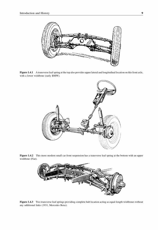
Figure 1.4.1 A transverse leaf spring at the top also provides upper lateral and longitudinal location on this front axle,

with a lower wishbone (early BMW).

Figure 1.4.2 This more modern small car front suspension has a transverse leaf spring at the bottom with an upper

wishbone (Fiat).

Figure 1.4.3 Two transverse leaf springs providing complete hub location acting as equal-length wishbones without

any additional links (1931, Mercedes Benz).


1.5 Early Independent Fronts

Through the 1920s, the rigid axle at the front was increasingly a problem. Despite considerable thought

and experimentation by suspension design engineers, no way had been found to make a steering system

that worked accurately. In other words, there were major problems with bump steer, roll steer and

spring wind-up, particularly during braking. Any one of these problems might be solved, but not all at

once. With increasing engine power and vehicle speeds, this was becoming increasingly dangerous, and

hard front springs were required to ameliorate the problem, limiting the axle movement, but this caused

very poor ride comfort. The answer was to use independent front suspension, for which a consistently

accurate steering system could be made, allowing much softer springs and greater comfort. Early

independent suspension designswere produced byAndr�eDubonnet in France in the late 1920s, and a littlelater for Rolls-Royce by Donald Bastow and Maurice Olley in England. These successful applications of

independent suspension became known in the USA, and General Motors president Alfred P. Sloan took

action, as he describes in his autobiography (Sloan, 1963).

Around 1930, Sloan considered the problem of ride quality as one of the most pressing and most

complex in automotive engineering, and the problemwas gettingworse as car speeds increased. The early

solid rubber tyres had been replaced by vented thick rubber, and then by inflated tyres. In the 1920s, tyres

became even softer, which introduced increased problems of handling stability and axle vibrations. On a

trip to Europe, Sloan met French engineer Andr�e Dubonnet who had patented a successful independent

suspension, and had him visit the US to make contact with GM engineers. Also, by 1933 Rolls-Royce

already had an independent front suspension, whichwas on cars imported to theUSA.MauriceOlley, who

had previously worked for Rolls-Royce, was employed by GM, and worked on the introduction of

independent suspensions there. In Sloan’s autobiography, a letter fromOlley describes an early ridemeter,

whichwas simply an open-topped container of water, whichwasweighed after ameasuredmile at various

speeds. Rolls-Royce had been looking carefully at ride dynamics, including measuring body inertia,

trying to get a sound scientific understanding of the problem, andOlley introduced this approach atGM. In

1932 they built the K-squared rig (i.e. radius of gyration squared), a test car with various heavy added

masses right at the front and rear to alter the pitch inertia in a controlled way. This brought home the

realisation that a much superior ride could be achieved by the use of softer front springs, but soft springs

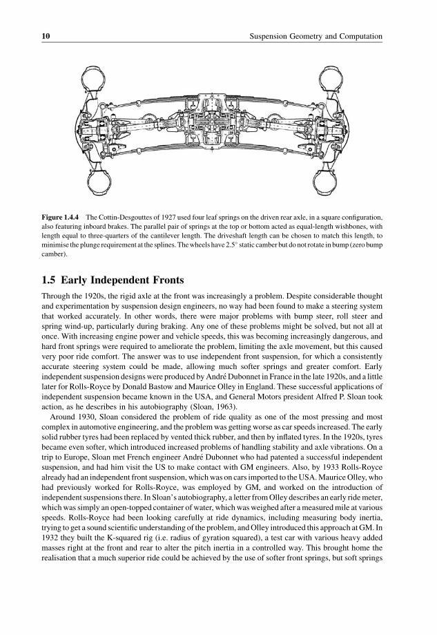
Figure 1.4.4 The Cottin-Desgouttes of 1927 used four leaf springs on the driven rear axle, in a square configuration,

also featuring inboard brakes. The parallel pair of springs at the top or bottom acted as equal-length wishbones, with

length equal to three-quarters of the cantilever length. The driveshaft length can be chosen to match this length, to

minimise the plunge requirement at the splines. Thewheels have2.5� static camber but donot rotate in bump (zero bump

camber).


caused shimmy problems and bad handling. Two experimental Cadillac cars were built, one using

Dubonnet’s type of suspension, the other with a double-wishbone (double A-arm) suspension of GM’s

design. The engineers were pleased with the ride and handling, but shimmy steering vibration was a

persistent problem requiring intensive development work. In March 1933 these two experimental cars

were demonstrated to GM’s top management, along with an automatic transmission. Within a couple of

miles, the ‘flat ride’ suspension was evidently well received.

March 1933was during the Great Depression, and financial constraints on car manufacturing and retail

prices were pressing, but the independent front suspension designs were enthusiastically accepted, and

shown to the public in 1934. In 1935 Chevrolet and Pontiac had cars available with Dubonnet

suspension, whilst Cadillac, Buick and Oldsmobile offered double-wishbone front suspension, and the

rigid front axlewas effectively history, for passenger cars at least. A serious concern for productionwas the

ability of the machine tool industry to produce enough suitable centreless grinders to make all the coil

springs that would be required.With some practical experience, it became apparent thatwith development

the wishbone suspension was easier and cheaper to manufacture, and also more reliable, and was

universally adopted.

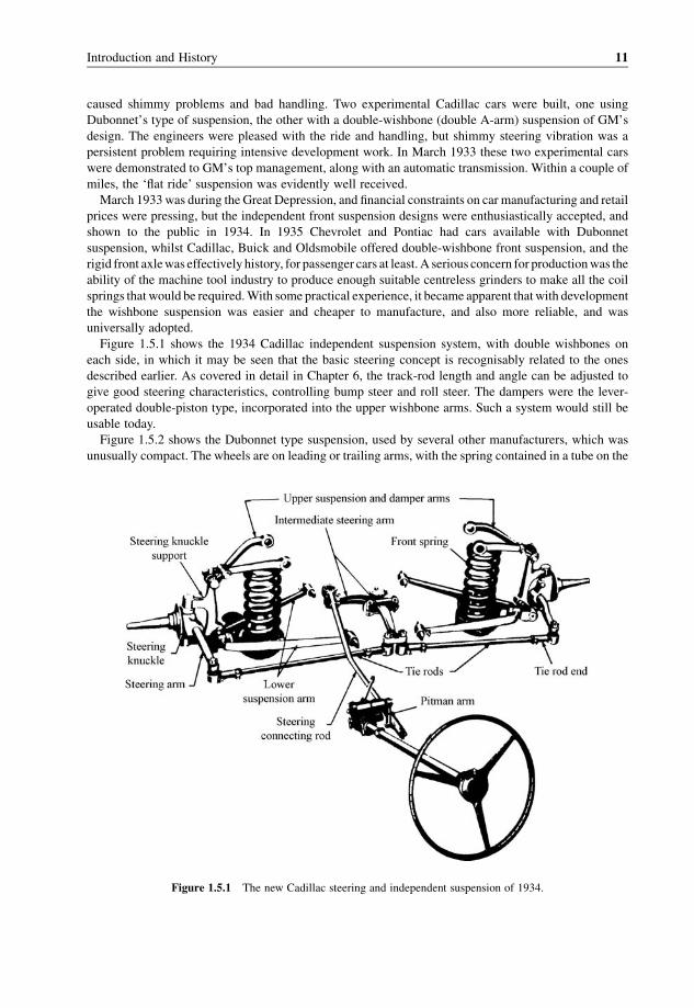
Figure 1.5.1 shows the 1934 Cadillac independent suspension system, with double wishbones on

each side, in which it may be seen that the basic steering concept is recognisably related to the ones

described earlier. As covered in detail in Chapter 6, the track-rod length and angle can be adjusted to

give good steering characteristics, controlling bump steer and roll steer. The dampers were the lever-

operated double-piston type, incorporated into the upper wishbone arms. Such a system would still be

usable today.

Figure 1.5.2 shows the Dubonnet type suspension, used by several other manufacturers, which was

unusually compact. The wheels are on leading or trailing arms, with the spring contained in a tube on the

Figure 1.5.1 The new Cadillac steering and independent suspension of 1934.


Figure 1.5.2 TheDubonnet type suspension in planview, front at the top: (a) with trailing links; (b) with leading links

(1938 Opel).

Figure 1.5.3 Broulhiet ball-spline sliding pillar independent suspension.


steerable part of the system. The type shown has a single tie rod with a steering box, as was usual then, but

the system is equally adaptable to a steering rack. The Ackermann effect is achieved here by angling the

steering arms backwards and inwards in Figure 1.5.2(a)with the trailing arms, or forwards and outwards in

Figure 1.5.2(b) with the leading arms. The steering action is entirely on the sprung mass, so there is no

question of bump or roll steer due to the steering, and there are no related issues over the length of the

steering members. Bump steer effects depend only on the angle of the pivot axis of the arms, in this case

simply transverse, with zero bump steer and zero bump camber. Other versions had this axis at various

angles. The leading link type at the front of a vehicle gives considerable anti-dive in braking, but is harsh

over sharp bumps. The trailing-arm version is better over sharp bumps but has strong pro-dive in braking.

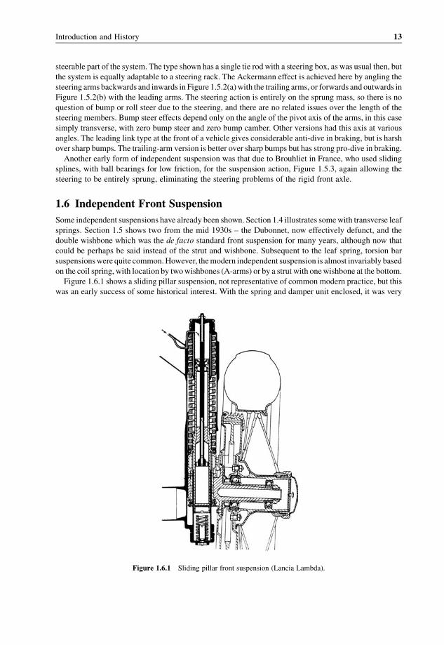
Another early form of independent suspension was that due to Brouhliet in France, who used sliding

splines, with ball bearings for low friction, for the suspension action, Figure 1.5.3, again allowing the

steering to be entirely sprung, eliminating the steering problems of the rigid front axle.

1.6 Independent Front Suspension

Some independent suspensions have already been shown. Section 1.4 illustrates somewith transverse leaf

springs. Section 1.5 shows two from the mid 1930s – the Dubonnet, now effectively defunct, and the

double wishbone which was the de facto standard front suspension for many years, although now that

could be perhaps be said instead of the strut and wishbone. Subsequent to the leaf spring, torsion bar

suspensionswere quite common.However, themodern independent suspension is almost invariably based

on the coil spring, with location by twowishbones (A-arms) or by a strut with onewishbone at the bottom.

Figure 1.6.1 shows a sliding pillar suspension, not representative of common modern practice, but this

was an early success of some historical interest. With the spring and damper unit enclosed, it was very

Figure 1.6.1 Sliding pillar front suspension (Lancia Lambda).


reliable, particularly compared with other designs of the early days. When introduced, this was regarded

by the manufacturer as the best suspension design regardless of cost.

Figure 1.6.2 shows various versions and views of the twin parallel-trailing-arm suspension, whichmost

often used torsion-bar springing in the cross tubes. On the Gordon-Armstrong this could be supplemented

with, or replaced by, coils springs used in compression with draw bars, with double action on the spring.

Again, thiswas a very compact system. The steering can be laid out to give zero bump steer, as in theAston

Martin version of Figure 1.6.2(d), or even with asymmetrical steering as in Figure 1.6.2(a).

A transverse single swing-arm type of front suspension can be used, as in Figure 1.6.3, but with lower

body pivot points than the usual driven rear swing axle, giving a lower roll centre. There is a large bump

camber effect with this design, such as to effectively eliminate roll camber completely. Steering is by

Figure 1.6.2 Parallel-trailing-arm front suspension: (a) general front view (VW); (b) rear three-quarter view of

torsion bar type construction; (c) parallel-trailing-arm suspension with laid-down compression coil spring and tension

bar (Gordon-Armstrong); (d) steering layout for parallel-trailing-arm system, plan view (early Aston Martin).


rack-and-pinion, with appropriately long track rods, giving no bump steer, this requiring the pick-up

points on the rack to be alignedwith the armpivot axes in the straight-ahead position. Unusually, the track-

rod connections are on the rear of the rack, which affects only the plan view angle of the track rods, and

hence the Ackermann factor.

The Glas Isar had double wishbones, as seen in Figure 1.6.4, but the upper wishbone had its pivot axis

transverse, so in front view the geometry was similar to a strut-and-wishbone suspension. The steering

system is high up, and asymmetrical. Analysis of bump steer requires a full three-dimensional solution, but

with the asymmetrical steering on this design there could be problems unless the track-rod connections to

the steering box arm are aligned with the upper wishbone axes.

Some early double-wishbone systems were very short, particularly on racing cars, as in Figure 1.6.5.

With the relatively long track rod shown there would have been significant bump steer, which could have

been only marginally acceptable by virtue of the stiff suspension and small suspension deflections. This

makes an interesting contrast with the very long wishbones on modern racing cars, although in that case

the deflections are still small and it is done for different reasons.

Figure 1.6.3 Single transverse swing-arm independent front suspension with rack-and-pinion steering (1963

Hillman).

Figure 1.6.4 A double-wishbone suspension in which the wishbone axes are crossed (Glas Isar).


Figure 1.6.6 shows an engineering section of a fairly representative double-wishbone system, with

unequal-length arms, nominally parallel in the static position. As is usual with double wishbones, the

spring acts on the lower arm at a motion ratio of about 0.5. The steering axis is defined by ball joints rather

than by the old kingpin system, with wide spacing giving lower joint loads.

In Figure 1.6.7, a more recent double-wishbone system, the upper wishbone is partially defined by the

rear-mounted anti-roll bar. The steering arms are inclined to the rear as if to give anAckermann effect, but

the track rods are also angled (seeChapter 5). The offset connections on the steering box and idler armgive

some Ackermann effect.

The modern double-wishbone system of Figure 1.6.8 is different in that the spring acts on the upper

wishbone,with vertical forces transmitted into the body at the top of thewheel arch in the sameway as for a

strut. However, despite the spring position this is certainly not a strut suspension, which is defined by a

Figure 1.6.5 An early double-wishbone system with very short arms (Mercedes Benz). The suspension spring is

inside the transverse horizontal tube.

Figure 1.6.6 Traditional configuration of passenger car double-wishbone suspension, with the spring and damper

acting on the lower wishbone (Jaguar).


rigid camber connection between thewheel upright and the strut. The steering connections are to the ends

of the rack, to give the correct track-rod length to control bump steer.

The commercial vehicle front suspension of Figure 1.6.9 is a conventional double-wishbone system

with a rear-mounted anti-roll bar, and also illustrates the use of a forward steering box and steep steering

Figure 1.6.7 A passenger car double-wishbone system with a wide-base lower wishbone, and the upper wishbone

partially defined by the anti-roll bar (Mercedes Benz).

Figure 1.6.8 A representativemodern double-wishbone suspension, with spring and damper acting on the upper arm

(Renault). This is not a strut suspension.


Figure 1.6.9 A double wishbone system from a light commercial vehicle, also illustrating a forward steering

system (VW).

Figure 1.6.10 MacPherson’s 1953 US patent for strut suspension (front shown).


column on this kind of vehicle. Again, the tie rod and idler arm allow the two track rods to be equal in

length and to have correct geometry for the wishbones.

Finally, Figure 1.6.10 shows the MacPherson patent of 1953 for strut suspension, propsed for use at

the front and the rear. A strut suspension is one inwhich thewheel upright (hub) is controlled in camber by

a rigid connection to the strut itself. This was popularised for front suspension during the 1950s and 1960s

by Ford, with the additional feature that the function of longitudinal location was combined with an

anti-roll bar. Strut suspension lacks the adaptability of double-wishbone suspension to desired geometric

properties, but can bemade acceptable whilst giving other benefits. The load transmission into the body is

Figure 1.6.11 Passenger car strut suspension with wide-based lower wishbone and low steering (VW).

Figure 1.6.12 Passenger car strut suspension with wide-based lower wishbone and high steering (Opel).


widely spread, and pre-assembled units of the suspension can be fitted to the body in an efficientmanner on

the final assembly line.

Figures 1.6.11 and 1.6.12 give two more modern examples, in fact of strut-and-wishbone suspensions,

normally just called strut suspensions, as now so commonly used on small and medium passenger

vehicles. The two illustrations show conventional struts. In contrast, a Chapman strut is a strut suspension

with a driveshaft, the shaft providing the lateral location of the bottommember, this requiring and allowing

no length change of the driveshaft, eliminating a number of problems such as sticking splines under load

(see Figure 1.10.7). In Figure 1.6.11 the steering rack is low, close to the level of the wishbone, and

the track-rod connections are, correspondingly, at the ends of the rack, to give the correct track-rod length.

In Figure 1.6.12 the steering is higher, at the level of the spring seat, so for small bump steer the track rods

must be longer, and are connected to the centre of the rack.

1.7 Driven Rigid Axles

The classic driven rigid rear axle, or so-called ‘live axle’, is supported and located by two leaf springs, in

which case it is called a ‘Hotchkiss axle’, as shown previously in Figures 1.3.5 and 1.3.6. Perhaps due to

the many years of manufacturers’ experience of detailing this design, sometimes it has been implemented

with great success. In other cases, there have been problems, such as axle tramp, particularly when high

tractive force is used. To locate the axle more precisely, or more firmly, sometimes additional links are

used, such as the longitudinal traction bars above the axle in Figure 1.7.1, opposing pitch rotation. These

used to be a well-known aftermarket modification for some cars, but were often of no help. In other cases,

the leaf springs have been retained as the sole locating members but with the springing action assisted by

coils, as in Figure 1.7.2, giving good load spreading into the body.

However, with the readier availability of coil springs, in due course the rear leaf-spring axle finally

disappeared from passenger cars, typically being replaced by the common arrangement of Figure 1.7.3,

with four locating links, this system being used by several manufacturers. The two lower widely-spaced

parallel links usually also carry the springs, as this costs less boot (trunk) space than placing them directly

on the axle. Lateral positioning of the axle is mainly by the convergent upper links, although this gives

rather a high roll centre. The action of axle movement may not be strictly kinematic, and may depend to

some extent on compliance of the large rubber bushes that are used in each end of the links.

The basic geometry of the four-link system is retained in the T-bar system of Figure 1.7.4, with the

cross-arm of the T located between longitudinal ribs on the body, allowing pivoting with the tail of the T,

connected to the axle, able to move up and down in an arc in side view. This gives somewhat more precise

location than the four-link system, and requires less bush compliance for its action, but again the roll centre

is high, satisfactory for passenger cars, but usually replaced by a sliding block system for racing versions

of these cars.

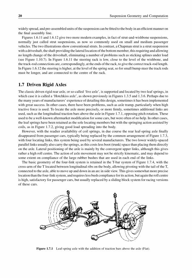
Figure 1.7.1 Leaf-spring axle with the addition of traction bars above the axle (Fiat).


Figure 1.7.3 Widely-used design of four-link location axle (Ford).

Figure 1.7.2 Leaf-spring axle with additional coil springs (Fiat).

Figure 1.7.4 Alfa-Romeo T-bar upper lateral location.


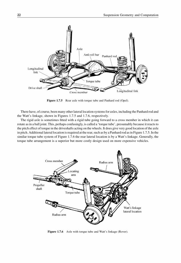
There have, of course, beenmanyother lateral location systems for axles, including the Panhard rod and

the Watt’s linkage, shown in Figures 1.7.5 and 1.7.6, respectively.

The rigid axle is sometimes fitted with a rigid tube going forward to a cross member in which it can

rotate as in a ball joint. This, perhaps confusingly, is called a ‘torque tube’, presumably because it reacts to

the pitch effect of torque in the driveshafts acting on thewheels. It does give very good location of the axle

in pitch.Additional lateral location is required at the rear, such as by a Panhard rod as in Figure 1.7.5. In the

similar torque tube system of Figure 1.7.6 the rear lateral location is by a Watt’s linkage. Generally, the

torque tube arrangement is a superior but more costly design used on more expensive vehicles.

Figure 1.7.5 Rear axle with torque tube and Panhard rod (Opel).

Figure 1.7.6 Axle with torque tube and Watt’s linkage (Rover).


Figure 1.8.1 De Dion axle: (a) front three-quarter view; (b) rear elevation; (c) plan view (1969 Opel).


1.8 De Dion Rigid Axles

ThedeDiondesign is an old onegoingback to the earliest days ofmotoring. In this axle, the twowheel hubs are

linked rigidly together, but the final drive unit is attached to the body, so the unsprung mass is greatly reduced

compared to a conventional live axle, Figure 1.8.1. Driveshaft length must be allowed some variation, for

example by splines. The basic geometry of axle location is the same as that of a conventional axle.

Figure 1.8.2 shows a slightly different version in which thewheels are connected by a large sliding tube

permitting some track variation, so that the driveshafts can be of constant length.

In general, the de Dion axle is technically superior to the normal live axle, but more costly, and so has

been found on more expensive vehicles.

1.9 Undriven Rigid Axles

Undriven rigid axles, used at the rear of front-drive vehicles, have the same geometric location

requirements as live rigid axles, but are not subject to the additional forces and moments of the drive

action, and can be made lower in mass. Figure 1.9.1 is a good example, with two lower widely-spaced

Figure 1.8.2 De Dion axle variation with sliding-tube variable track (1963 Rover).

Figure 1.9.1 Simple undriven rigid axle (Renault).


longitudinal arms and a single upper link for lateral and pitch location. The arms are linked by an anti-roll

bar. The roll centre is high.

In Figure 1.9.2, lateral location is by the long diagonal member. This form eliminates the lateral

displacements in bumpof the Panhard rod. If the longitudinal links are fixed rigidly to the axle then the axle

acts in torsion as an anti-roll bar, the system then being a limiting case of a trailing-twist axle.

The undriven axle of Figure 1.9.3 has location at each side by a longitudinal Watt’s linkage, giving a

truer linear vertical movement to thewheel centre thanmost systems, and also affecting the pitching angle

of the hub, introducing an axle torsion anti-roll bar effect, but in a non-linear way.

Figure 1.9.2 Undriven rigid axle with diagonal lateral location (Audi).

Figure 1.9.3 Undriven rigid axle with longitudinal Watt’s linkages and Panhard rod (Saab).


Figure 1.9.4 shows a system with trailing arms operating half-width torsion bars, and with a short

diagonal link for lateral location. If the trailing arms are fixed to the axle then in roll the axle will deflect

torsionally, giving an anti-roll bar effect,whilst the thin trailing armsdeflect relatively freely. This is another

example of a limiting case of a trailing-twist axle, with the cross member at the wheel position.

Figure 1.9.5 shows a modern rigid axle with location system designed to give controlled side-force

oversteer, the axle being able to yaw slightly about the front location point, according to the stiffness of the

bushes in the outer longitudinal members.

1.10 Independent Rear Driven

In the early days, most road vehicles had a rear drive, using a rigid axle. There were, however, some

adventurous designers who tried independent driven suspension, such as on the Cottin-Desgoutes, which

was shown in Figure 1.4.4. The most common early independent driven suspension was the simple swing

axle, which has the advantage of constant driveshaft lengths, and low unsprung mass. The driveshafts can

Figure 1.9.4 Rigid axlewith diagonal lateral location and torsionbar springing, planview (nascent trailing-twist axle)

(Citro€en).

Figure 1.9.5 Tubular-structure undriven rigid axle with forward lateral location point and two longitudinal links

(Lancia).


swing forward so they require some extra location. Initially, a simple longitudinal pivot was used.

Sometimes the supporting member had pivot points both in front of and behind the driveshaft.

Figure 1.10.1 shows one with a single, forward, link. The swing axle has a large bump camber and

little roll camber. The roll centre is not as high aswithmany rigid axles, but it is more of a problem because

with a high roll centre on independent suspension there is jacking, which in extremis can get out of control

with the outer wheel tucking under.

To overcome the problem of the roll centre of the basic swing axle, a low-pivot swing axle may be used,

as in Figure 1.10.2, now requiring variable-length driveshafts by splines or doughnuts. The bottom pivots

are offset slightly, longitudinally. This is still considered to be a swing axle because the axis of pivot of the

axle part is longitudinal.

The obvious alternative to the swing axle is to use simple trailing arms,with the pivot axis perpendicular

to the vehicle centre plane and parallel to the driveshafts. Again, this requires allowance for length

Figure 1.10.1 Swing axle with long leading links for longitudinal location (Renault).

Figure 1.10.2 Low-pivot swing axle with inboard brakes (Mercedes Benz).


variation, a significant complication, Figure 1.10.3. In the example shown, the springing is by half-width

torsion bars anchored at the vehicle centreline. There is also an anti-roll bar.

The next development, introduced in 1951, was the semi-trailing arm in which the arm pivot axis is a

compromise between the swing axle and the plain trailing arm, typically in the range 15� to 25�, as inFigure 1.10.4. A more recent and simpler semi-trailing arm system is shown in Figure 1.10.5. Bump

camber is greatly reduced compared with the swing axle.

To control the geometric properties more closely to desired values, a double wishbone system may be

used, although this is less compact and on the rear of a passenger car it is detrimental to luggage space, but

it is very widely used on sports and racing cars. Figure 1.10.6 shows an example sports car application,

where the camber angle and the roll centre height were made adjustable.

Figure 1.10.3 Plain trailing arms with 90� transverse axis of pivot (Matra Simca).

Figure 1.10.4 Thefirst semi-trailing-armdesign, alsowith transaxle and inboard brakes: (a) planview; (b) front three-

quarter view (1951 Lancia).


The Chapman strut is a strut suspension in which the lower lateral location is provided by a fixed-length

driveshaft. Figure 1.10.7 gives an example. Lower longitudinal location must also be provided, as seen in

the forward diagonal arms which also, here, carry the springs.

Figure 1.10.8 shows the ‘Weissach axle’, which uses controlled compliance to give some toe-in on

braking, or on power lift-off, for better handling.

A relatively recent extension of the wishbone concept is to separate each wishbone into two separate

simple links. There are then five links in total, two for eachwishbone and one steer angle link. This system

Figure 1.10.5 Semi-trailing arms (BMW).

Figure 1.10.6 Double-wishbone sports car suspension with diagonal spring–damper unit, roll centre height

dimensions in inches (Ford).


Figure 1.10.7 Chapman strut with front link for longitudinal location: (a) rear elevation; (b) front three-quarter view

(Fiat).

Figure 1.10.8 ‘Weissach axle’ (Porsche).


has been used at the front and the rear, and, with careful design, makes possible better control of the

geometric and compliance properties. Figure 1.10.9 shows an example. The advantages seem real for

driven rear axles, but undriven ones have not adopted this scheme. The concept has also been used at the

front for steered wheels.

Figure 1.10.9 Five-link (‘multilink’) suspension: (a) complete driven rear-axle unit; (b) perspective details of one

side with plan and front and side elevations (Mercedes Benz).


1.11 Independent Rear Undriven

At the rear of a front-drive vehicle it seems quite natural and easy to use independent rear suspension.

Figures 1.11.1–1.11.4 give some examples.

The plain trailing arm with transverse pivot at 90� to the vehicle centre plane has often been used. Theoriginal BMC Mini, on which it was used in conjunction with rubber suspension, was a particularly

compact example. A subframe is often used, as seen in Figure 1.11.1. Vertical coil springs detract from the

luggage compartment space, so torsion bars are attractive. For symmetry, these have a length of only

half of the track (tread), which is less than ideal. Figure 1.11.2 shows an examplewhere slightly offset full-

length bars are used. The left and right wheelbases are slightly different, but this does not seem to be of

practical detriment.

Figure 1.11.1 Plain trailing arms, 90� pivot axis, coil springs (Simca).

Figure 1.11.2 Plain trailing arms, 90� pivot axis, offset torsion-bar springs, unequal wheelbases (Renault).


Figure 1.11.3 shows an independent strut rear suspension, the wheel-hub camber and pitch being

controlled by the spring–damper unit. Twin lateral arms control scrub (track change) and the steer angle.

The anti-roll bar has no effect on the geometry. Figure 1.11.4 shows another strut suspension, with a single

wide lateral link controlling the steer angle.

Figure 1.11.3 Strut suspension with long twin lateral/yaw location arms and leading link for longitudinal location

(Lancia).

Figure 1.11.4 Strut suspension with wide lateral links and longitudinal links (Ford).


1.12 Trailing-Twist Axles

The ‘trailing-twist’ axle, now often known as the ‘compound-crank’ axle, is illustrated in

Figures 1.12.1–1.12.3. The axle concept is good, but the new name is not an obvious improvement

over the old one. This design is a logical development of the fully-independent trailing-arm system.

Beginningwith a simple pair of trailing arms, it is often desired to add an anti-roll bar. Originally, this was

done by a standard U-shaped bar with twomountings on the body locating the bar, but allowing it to twist.

Drop links connected the bar to the trailing arms. A disadvantage of this basic systemwas that the anti-roll

bar transmitted extra noise into the passenger compartment, despite being fitted with rubber bushes. This

problem was reduced by deleting the connections to the body, instead using two rubber-bushed

connections on each trailing arm, so that the bar was still constrained in torsion. This was then simplified

Figure 1.12.1 A compound crank axle using torsion-bar springs (Renault).

Figure 1.12.2 A compound crank axle with coil springs (Opel).


mechanically by making the two arms and the bar in one piece, requiring the now only semi-independent

axle to flex in bending and torsion. This complicated the geometry, but allowed a compact system that was

easy to install as a prepared unit at the final assembly stage. As seen in the figures, to facilitate the

necessary bending and torsion the cross member of the axle is an open section pressing. The compound

crank axle is now almost a standard for small passenger cars.

1.13 Some Unusual Suspensions

Despite the wide range of conventional suspensions already shown, many other strange and unusual

suspensions have been proposed, and patented, and some actually used, on experimental vehicles at least,

the designers claiming better properties of one kind or another, sometimes with justification. For most

vehicles, the extra complication is not justified. Some designs are presented here for interest, and as a

stimulus for thought, in approximate chronological order, but with no endorsement that they all work as

claimed by the inventors. Proper design requires careful consideration of equilibrium and stability of the

mechanism position, the kind of analysis which is usually conspicuously lacking from patents, which are

generally presented in vague qualitative and conceptual terms only. As the information about these

suspensions is mainly to be found in patent applications, engineering analysis is rarely offered in their

support, the claims are only qualitative. The functioning details of actual roll angles and camber angles and

the effect on handling behaviour are not discussed in the patents in any significant way.

There aremany known designs of suspensionwith supplementary roll-camber coupling, that is, beyond

the basic roll camber normally occurring. So far, however, this has not been a very successful theme. The

Figure 1.12.3 A compound crank axle similar to that in Figure 1.12.2, also showing in (a) the body fixture brackets,

and in (b) the front elevation (Opel).


proposed systems add cost, weight and complexity, and often have packaging difficulties. Also, there does

not appear to have been a published analysis of the vehicle-dynamic handling consequences of such

systems to provide an adequate basis for design. Typically, where the expected use is on passenger

vehicles, the intention is to reduce or eliminate body roll, or even to bank the body into the corner, with

claims of improved comfort. Where racing applications are envisaged, the main concern is elimination of

adverse camber in roll.

Most of the suspensions discussed are of pure solidmechanical design. Such suspension design tends to

add undesirable weight, is usually bulky, and is therefore space-consuming with packaging problems.

Camber adjustment accomplished by lateralmovement of the lower suspension arms causes adverse scrub

effects at the tyre contact patch which is probably not acceptable.

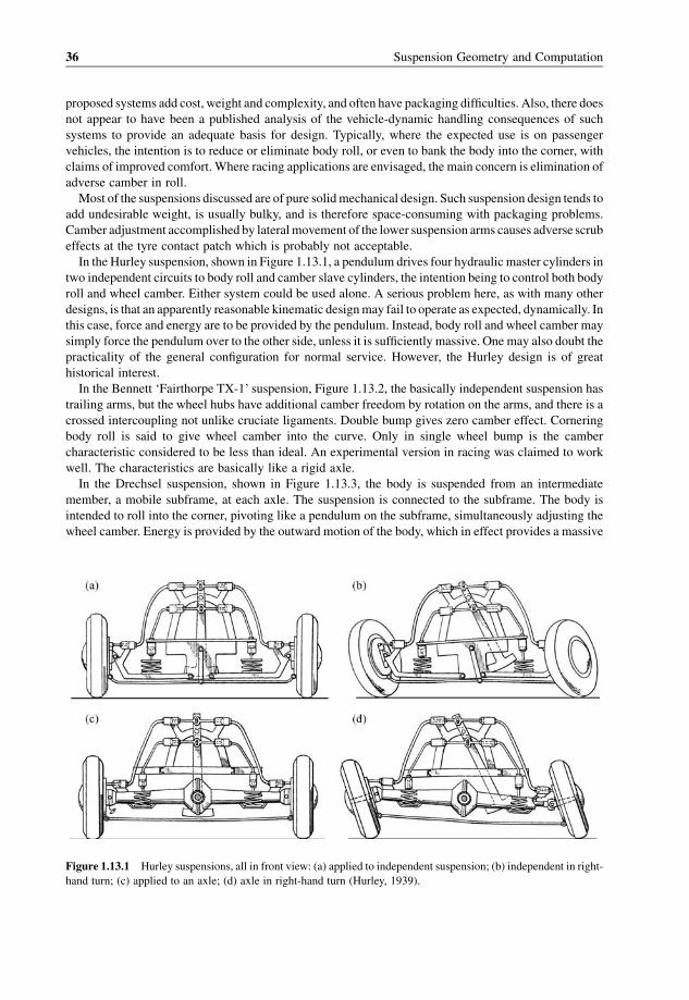
In the Hurley suspension, shown in Figure 1.13.1, a pendulum drives four hydraulic master cylinders in

two independent circuits to body roll and camber slave cylinders, the intention being to control both body

roll and wheel camber. Either system could be used alone. A serious problem here, as with many other

designs, is that an apparently reasonable kinematic designmay fail to operate as expected, dynamically. In

this case, force and energy are to be provided by the pendulum. Instead, body roll and wheel camber may

simply force the pendulum over to the other side, unless it is sufficiently massive. One may also doubt the

practicality of the general configuration for normal service. However, the Hurley design is of great

historical interest.

In the Bennett ‘Fairthorpe TX-1’ suspension, Figure 1.13.2, the basically independent suspension has

trailing arms, but the wheel hubs have additional camber freedom by rotation on the arms, and there is a

crossed intercoupling not unlike cruciate ligaments. Double bump gives zero camber effect. Cornering

body roll is said to give wheel camber into the curve. Only in single wheel bump is the camber

characteristic considered to be less than ideal. An experimental version in racing was claimed to work

well. The characteristics are basically like a rigid axle.

In the Drechsel suspension, shown in Figure 1.13.3, the body is suspended from an intermediate

member, a mobile subframe, at each axle. The suspension is connected to the subframe. The body is

intended to roll into the corner, pivoting like a pendulum on the subframe, simultaneously adjusting the

wheel camber. Energy is provided by the outward motion of the body, which in effect provides a massive

Figure 1.13.1 Hurley suspensions, all in front view: (a) applied to independent suspension; (b) independent in right-

hand turn; (c) applied to an axle; (d) axle in right-hand turn (Hurley, 1939).


pendulum as an improvement to the Hurley separate-pendulum concept. There are two geometric roll

centres, one for the body on the subframe, the other for the suspension on the subframe.

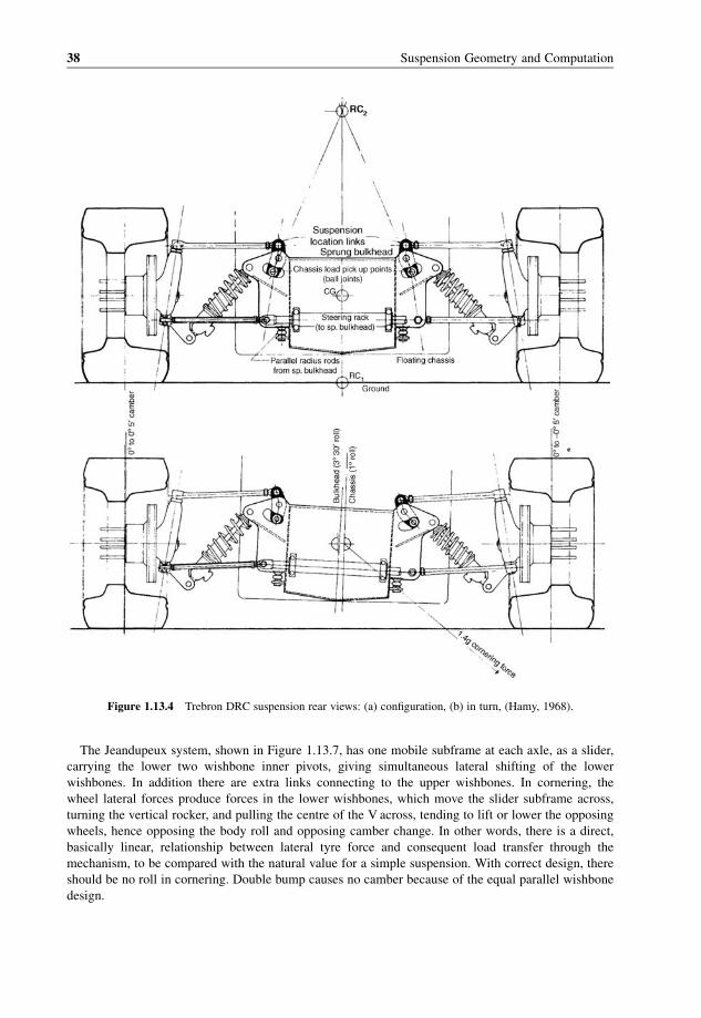
TheTrebron double roll centre (DRC) suspension, Figure 1.13.4, due toN.Hamy, is similar in operation

to the Drechsel concept, but with changes to the details. An adapted passenger car test vehicle operated

successfully, demonstrating negated chassis roll and camber change in cornering.

In the Bolaski suspension, shown in Figure 1.13.5, the operating principle is again similar to that of

Drechsel, using the body as amassive pendulum, but in this case themain body rests on compression links,

and in cornering is intended to deflect the central triangular member which in turn adjusts the wheel

camber by the lower wishbones. Bolaski limits his invention for application to front suspensions by the

title of this patent.

In the Parsons system, Figure 1.13.6, each axle has two mobile subframes. The body and the two

subframes have a common pivot as shown, but this is not an essential feature. The front suspension design

is expected to use struts. Each upper link, on rising in bump, pulls on the opposite lower wishbone,

changing the camber angle of that side.On the rear suspension design,with doublewishbones, in bump the

rising lower link pushes the opposite upper wishbone out, having the same type of camber effect. In the

double-wishbone type shown, the spring as shownwould give a negative heave stiffness, but this would be

used in conjunction with a pair of stiff conventional springs to give an equivalent anti-roll bar effect. Of

course, the springs shown are not an essential part of the geometry.

Figure 1.13.3 Drechsel suspension, rear view, left-hand cornering (Drechsel, 1956).

Figure 1.13.2 ‘Fairthorpe TX-1’ suspension (T. Bennett, 1965).


The Jeandupeux system, shown in Figure 1.13.7, has one mobile subframe at each axle, as a slider,

carrying the lower two wishbone inner pivots, giving simultaneous lateral shifting of the lower

wishbones. In addition there are extra links connecting to the upper wishbones. In cornering, the

wheel lateral forces produce forces in the lower wishbones, which move the slider subframe across,

turning the vertical rocker, and pulling the centre of the V across, tending to lift or lower the opposing

wheels, hence opposing the body roll and opposing camber change. In other words, there is a direct,

basically linear, relationship between lateral tyre force and consequent load transfer through the

mechanism, to be compared with the natural value for a simple suspension. With correct design, there

should be no roll in cornering. Double bump causes no camber because of the equal parallel wishbone

design.

Figure 1.13.4 Trebron DRC suspension rear views: (a) configuration, (b) in turn, (Hamy, 1968).


In contrast to the earlier suspensions, all claimed to be passive in action, the Phillippe suspension,

Figure 1.13.8, is declared to be an active system with power input from a hydraulic pump, with camber

control by hydraulic action on a slider linking the inner pivots of the upper wishbones. This is direct active

control of the geometry, quite different from the normal active suspension concept which replaces the usual

springs anddampers in thevertical action of the suspension.The light pendulumshownacts only as a sensor.

Figure 1.13.5 Bolaski suspension (Bolaski, 1967).

Figure 1.13.6 Parsons suspensions: (a) for the steerable front using struts; (b) for the driven rear using double

wishbones. Additional springs and dampers would be used on each wheel (Parsons, 1971).


Figure 1.13.7 Jeandupeux suspension: (a) configuration; (b) kinematic action in bump and roll without camber

change (Jeandupeux, 1971).

Figure 1.13.8 (a) Phillippe suspension (Phillippe, 1975). (b) Variations of Phillippe suspension.


The Pellerin suspension is aimed specifically at formula racing cars which use front suspensions which

are very stiff in roll. These have sometimes used a mono-spring–damper suspension, the so-called

‘monoshock’ system, which is a suspension with a single spring–damper unit active in double bump, with

nominally no roll action in the suspensionmechanism itself. The complete front roll stiffness then depends

mainly on the tyre vertical stiffness with some contribution from suspension compliance. In the Pellerin

system, Figure 1.13.9, the actuator plate of the spring–damper unit is vertically hinged, allowing some

Figure 1.13.9 Pellerin suspension (Pellerin, 1997).

Figure 1.13.10 Weiss PRCC suspension (springs not shown): (a) version 1, camber cylinders in wishbones; (b)

version 2, camber cylinder between the two wishbone pivots (Weiss, 1997).


lateral motion of the pushrod connection point. The roll stiffness of the suspension mechanism is then

providedby the tension in the hinged link, and is dependent on the basic pushrod compression force,which

increases with vehicle speed due to aerodynamic downforce.

The Weiss passive roll-camber coupled (PRCC) system, shown in Figure 1.13.10, uses hydraulic

coupling of thewheel camber anglewith body roll, in several configurations. Normal springs are retained.

Essentially, in cornering the tyre side forces are used to oppose body roll, and body forces oppose adverse

camber development, mediated by the hydraulics. Simple double bump moves the diagonal bump

cylinders, but these are cross coupled, so in this action they merely interchange fluid.

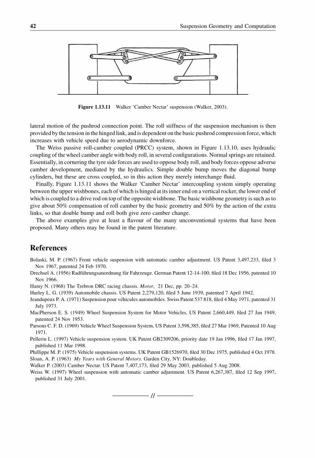
Finally, Figure 1.13.11 shows the Walker ‘Camber Nectar’ intercoupling system simply operating

between the upperwishbones, each of which is hinged at its inner end on a vertical rocker, the lower end of

which is coupled to a drive rod on top of the oppositewishbone. The basic wishbone geometry is such as to

give about 50% compensation of roll camber by the basic geometry and 50% by the action of the extra

links, so that double bump and roll both give zero camber change.

The above examples give at least a flavour of the many unconventional systems that have been

proposed. Many others may be found in the patent literature.

References

Bolaski, M. P. (1967) Front vehicle suspension with automatic camber adjustment. US Patent 3,497,233, filed 3

Nov 1967, patented 24 Feb 1970.

Drechsel A. (1956) Radf€uhrungsanordnung f€ur Fahrzeuge. German Patent 12-14-100, filed 18 Dec 1956, patented 10

Nov 1966.

Hamy N. (1968) The Trebron DRC racing chassis. Motor, 21 Dec, pp. 20–24.

Hurley L. G. (1939) Automobile chassis. US Patent 2,279,120, filed 5 June 1939, patented 7 April 1942.

Jeandupeux P. A. (1971) Suspension pour v�ehicules automobiles. Swiss Patent 537 818, filed 4May 1971, patented 31

July 1973.

MacPherson E. S. (1949) Wheel Suspension System for Motor Vehicles, US Patent 2,660,449, filed 27 Jan 1949,

patented 24 Nov 1953.

Parsons C. F. D. (1969) Vehicle Wheel Suspension System, US Patent 3,598,385, filed 27 Mar 1969, Patented 10 Aug

1971.

Pellerin L. (1997) Vehicle suspension system. UK Patent GB2309206, priority date 19 Jan 1996, filed 17 Jan 1997,

published 11 Mar 1998.

Phillippe M. P. (1975) Vehicle suspension systems. UK Patent GB1526970, filed 30 Dec 1975, published 4 Oct 1978.

Sloan, A. P. (1963) My Years with General Motors. Garden City, NY: Doubleday.

Walker P. (2003) Camber Nectar. US Patent 7,407,173, filed 29 May 2003, published 5 Aug 2008.

Weiss W. (1997) Wheel suspension with automatic camber adjustment. US Patent 6,267,387, filed 12 Sep 1997,

published 31 July 2001.

————— // —————

Figure 1.13.11 Walker ‘Camber Nectar’ suspension (Walker, 2003).


2

Road Geometry

2.1 Introduction

The purpose of a vehicle is to go from A to B, moving the passengers or payload comfortably, safely

and expediently. Considering in general any surface of the globe, the terrain to be covered may vary

enormously. In fact, most of the Earth’s ground surface is difficult terrain for a conventional motor vehicle

due to roughness, swampiness, etc. Specialised ground vehicles are required over much of the area, in

some cases tracked, in less difficult cases a good all-wheel-drive vehicle. Obviously, to ease the problem

the surface has been improved along many frequently-used routes, with a vast capital investment in roads

which generally have a broken rock base and are surfaced with concrete in some cases, or with fine gravel

held together by very high viscosity tar.

The general form of the ground and roads varies greatly, asmay readily be seen by studying a roadmap.

Figure 2.1.1(a) shows the contour map of a small section of Belgian pav�e type rough road surface made

with stone blocks, whichmay be contrasted with the relatively smooth nature of good quality roads such a

motorways. Figure 2.1.1(b) shows a theoretically generated isotropic surfacewhich is of similar character.

The shape of a road or desired path may be analysed in various ways, largely dependent on the

application. In handling analysis, the general geometric form is required, for example the path lateral

curvature, which governs the lateral tyre force requirement. On the other hand, in ride quality analysis it is

usual to think in terms of a Fourier spectral analysis of the road surface quality. This chapter deals

primarily with road geometry in conventional geometric terms, as is of use in performance and handling

analysis. The next chapter deals with the finer scale vertical perturbations of importance in comfort (ride

quality) analysis.

In general, the ground surface is defined by some sort of coordinate system. The Earth itself is a close

approximation to spherical, the sea-level reference surface being a slightly oblate spheroid due to the

diurnal rotation. The mean radius is 6371 km (SI units are described in Appendix B). The highest

mountain, Everest, is 8848 m above sea level, barely one-thousandth of the Earth’s radius. Locally, a

simple rectangular coordinate systemmay be used. The ISOvehicle-dynamics systemhasX forwards,Y to

the left andZ upwards. Consider, then, (X,Y) Earth-fixed coordinates, with the ground altitudeZ, relative to

some defined reference plane, such as notional local sea level, being a function of X and Y, as in

Figure 2.1.2. (The notation used in each chapter is summarised in Appendix A.) In principle, this

effectively fully defines the surface shape, excepting the extreme case of overhangs, where Z is

multivalued. The ground is notionally a continuum, although really discrete at the molecular level. In

any case, the surface would normally be represented in a digital form of Z(X,Y) values. With modern

computation, thememory size available is large, and good resolution of ground shape is possible, obtained

by satellite global-positioning systems and other means.


Nevertheless, the quality of the ground surface itselfmay be considered to be a separate feature from the

geographical ground shape, the distinction being at the scale depending on the vehicle, and is analysed for

its effect on tyre grip and ride quality rather than handling requirements. Thus the road shape on a small

scale, called the macrostructure and microstructure, which affects the tyre grip and aquaplaning, is

handled separately, as detailed in the next chapter.

Once a particular route is selected over the terrain, the nature of the representation of the surface

changes. In general, the road is definedby a band, of varyingwidth, along the surface of theEarth. The road

surface is then a section of the complete surface, its edges being the limits of the usable surface. In a

Figure 2.1.1 Road contour maps: (a) MIRA Belgian pav�e test track; (b) theoretically generated isotropic surface.

Long dashes are contours below datum, short ones above (Cebon and Newland, 1984).

Figure 2.1.2 General ground surface height Z above the datum plane is a function of rectangular coordinates (X,Y).


simpler representation, the road shape then becomes a single path line, essentially a function of one

variable rather than two, defined by values as a function of distance along the road, the path length from a

reference point.

The actual path of the vehicle centre of mass, or other reference point, projected down into the road

surface, gives a specific line. The path is like a bent wire in space, with curvature at any position on its

length. In the context of racing, this should be the ideal lap line forming a closed loop, but compromised in

reality by driver and vehicle imperfection and inconsistency, and by the requirement to avoid other

vehicles.

2.2 The Road

In plan view, the route from A to B is simplistically defined by a line, Figure 2.2.1, specified by a definite

relationship betweenX andY. In general, the functionsX(Y) and Y(X) are not single-valued.Measuring the

vehicle’s position by the distance travelled from the point A (i.e. the path length from A), then there is a

parametric representation of the route position, X(s) and Y(s). For a given path length s (i.e. position along

the road), various values may be deduced from the general surface shape, inter alia those in Table 2.2.1.

Strictly, the path length includes vertical positional variations, so the path length seen in the horizontal

(X,Y) plane is really

sH ¼ðBA

cos uRds

where uR is the road longitudinal gradient angle.

The longitudinal slope gives a longitudinal weight force component affecting the tractive force required

for steady speed. The banking slope similarly introduces a lateral component of the weight force. The

longitudinal normal curvature, combined with the speed, gives vertical accelerations which cause

variations of the tyre normal forces. The longitudinal lateral curvature creates the cornering force

requirement. The banking curvature affects tyre camber angles. The road camber twist (spatial rate of

change of bank angle) affects the tyre normal forces (diagonal distribution of normal force). The rate of

change of lateral curvature is the path turn-in, discussed later.

Figure 2.2.1 Route A to B specified by a line in coordinates (X,Y).

Road Geometry 45

The basic geometric properties in Table 2.2.1 require careful definition because the values obtained

depend in general on the resolution of the data, or of the wavelength filtering applied, which must be

chosen to suit the application. As an example, a pot-hole in a road may have an extreme slope at an edge,

but this would not generally be interpreted as a road slope in the general sense, but as a local disturbance.

In principle, the geometric shape of the road is continuous with wavelength, and if subject to Fourier

analysis may be represented in a form of spectral analysis, with no special significance for any particular

wavelengths. This is correct geometrically, but not true dynamically. The vehicle itself has a definite size,

as do thewheels and tyres, and the vehicle on its suspension has natural frequencies, and a speed of travel,

from which it is apparent that certain wavelengths may be significant. In particular, there is a dividing

frequency, not extremely well defined, which is some fraction of the natural heave frequency of the

vehicle. This dividing frequency separates road shapes which are dynamic in effect from those which are

essentially static in effect. In other words, in general, driving over a hill is not the same as driving over a

bump. For a passenger car, the basic natural frequency of the vehicle in heave, the basic ride frequency, is

typically about 1.4 Hz (8.8 rad/s). At a forward velocity of 20m/s, this corresponds to a resonant

wavelength of 14 m. For frequencies less than about 0.2 times the natural ride frequency there is no

significant dynamic effect, so wavelengths greater than about 5� 14m¼ 70m do not stimulate any

dynamic response. Therefore they can be separated out and dealtwith by differentmethods.A humpwith a

wavelength of 100 m is a small hill, not a ride or handling issue.

From this consideration, then, the geometric properties of the road are, in practice, separated out by

wavelength into static and dynamic factors, although this is not inherent in the basic geometric

specification of the road.

The altitude graph Z(s) is the longitudinal profile of the road as a function of distance along the road,

Figure 2.2.2. Thismay be derived conceptually fromFigures 2.1.2 and 2.2.1. Of course, inmany cases this

would actually be obtained directly, for example by driving the routewith instrumentation (a logger, GPS,

etc.), rather than by actual calculation from the general topological form ZR(X,Y).

The local road angles are defined as follows, as seen in Figure 2.2.3. For a given point on the path, there

is a plane tangential to the road surface at that point, generally not horizontal. The path lies locally in that

plane; draw the normal and tangent of the path which lie in that plane. Consider the longitudinal vertical

plane containing the tangent line. This is also simply the vertical plane tangent to the path at the point of

analysis. In this longitudinal vertical plane, the tangent line is at angle uR to the horizontal. This is the road

pitch angle (gradient angle) uR considered positive for an upward (climbing) gradient. The longitudinal

road gradient is actually

G ¼ sin uR ¼ dZR

ds

Table 2.2.1 The basic geometrical properties of a road, at a path point s

(1) the X coordinate

(2) the Y coordinate

(3) the road height (altitude) ZR(4) the usable width

(5) the longitudinal slope, angle uR(6) the banking (lateral) slope, angle fR

(7) the longitudinal normal curvature, kN(8) the longitudinal lateral curvature, kL(9) the banking (camber) curvature, kB(10) the road camber twist

(11) rate of change of lateral curvature

(12) etc.


Nowconsider the line normal to the path, in the road tangent plane. By rotating this normal line about an

axis along the path tangent line, the former may be brought to a horizontal position, that is, into the

horizontal plane. The angular displacement required to achieve this is the road bank angle. Note that the

bank angle is strictly measured in a plane perpendicular to the tangent line, not in a vertical plane.

Expressed in another way, the road bank rotation is about the tangent line axis, in general not about a

horizontal line.

This relates to the positional Euler angles of a vehicle body, which use yawing, pitching and rolling

angular displacements in that sequence about the vehicle-fixed (x,y,z) axes.

In practice, for cars, the path longitudinal slope is fairly small. One-in-seven is a considerable slope by

normal road standards (8.2�), and one-in-five is extreme (11.5�), so the road bank angle can normally be

approximatelymeasured in thevertical plane.However, the equations of road geometry are strictly correct

for the formal definition of the bank angle, not the approximation in the vertical plane. This is one of the

problems of combined gradient and banking. Considering verticals dropped from the path to a true

Figure 2.2.2 The road profile ZR(s) shows the path height as a function of path position.

Figure 2.2.3 Road angle geometry. The plane is that of the road surface at the point, containing the path line at the

point.

Road Geometry 47

horizontal plane, at the datum level, the result can be seen to be that the path elevation ZR may be plotted

against path position, giving ZRðsHÞ. The path slope is normally sufficiently small for this to be a minor

distinction, locally at least (e.g. cos 8� ¼ 0.99027). Mathematically, the gradient is

G ¼ dZR

ds

whereas numerically the mean gradient between two data points is

Gr ¼ ZR;r � ZR;r�1

sr � sr�1

It may be that the above expression givesGr�1. The gradient belongs to the space between the two points,

but may be attributed to one or other point. This is just a matter of definition.

2.3 Road Curvatures

Anypath curvature,k (lower caseGreek kappa, unitsm�1) is the reciprocal of the local radius of curvature,

R (m). (Use of the Greek alphabet is described in Appendix C.)

For a flat horizontal road with path radius R there is therefore simply a lateral curvature

kL ¼ 1

R

For a ‘straight’ road, in the sense of no corners or banking, but with undulations of road elevation, the

road gradient is

G ¼ dZR

ds

and the vertical curvature is defined as

kV ¼ dG

ds¼ d2ZR

ds2

with corresponding numerical definitions. In this case, with no road bank angle, and smallG, the vertical

curvature is the same as the normal curvature.

In the general case, the vehicle path line has lateral (cornering) curvature on a banked road which also

has longitudinal gradient. It is then necessary to consider five curvatures and two angles (see Figure 2.3.1

and Table 2.3.1).

Table 2.3.1 Path curvatures and angles, Figure 2.3.1

(1) k, the total path curvature

(2) kN, the normal curvature

(3) kL, the lateral curvature

(4) kV, the vertical curvature(5) kH, the horizontal curvature(6) fR, the road bank angle

(7) fk, the curvature vector angle from horizontal.


From Figure 2.3.1, the total curvature k can be resolved into perpendicular components. There are two

principal ways to do this. In the Earth-fixed datum coordinates, the horizontal and vertical components are

kH ¼ k cosfk

kV ¼ k sin fk

In the road-surface-aligned coordinates, the lateral and normal components are

kL ¼ k cos ðfk þ fRÞkN ¼ k sin ðfk þ fRÞ

The horizontal curvature kH is the curvature appearing in a road map (i.e. in plan view) with the

particular path drawn in.

The vertical curvature kV is the curvature derived from the path elevation graph ZRðsÞ.The normal curvature kN, the curvature normal to the track surface, is the one which affects the

symmetrical suspension deflections and the tyre vertical forces.

The lateral curvature kL, parallel to the local road surface, is the curvature requiring lateral tyre forcesfor the car to follow the road, and causing the vehicle roll angles.

In view of the above, dynamic analysis is most conveniently performed in coordinates aligned with the

banked track surface, and with the ðkN; kLÞ curvature pair, that is, with the normal and lateral curvatures.

For simulation purposes, it is necessary to know the road bank anglefR, and the curvature vector (i.e. kand fk, or other combination of data allowing k and fk to be evaluated). Methods of determining this

information are considered later.

The dynamic behaviour of the vehicle is normally analysed in road surface-aligned coordinates. These

are distinct from the Frenet–Serret coordinates generally used bymathematicians to analyse a curved line

in space (see Appendix E).

2.4 Pitch Gradient and Curvature

Consider a track with no bank angle, but with longitudinal gradient angle uR, as in Figure 2.4.1. The angleis considered constant, that is, the pitch curvature is temporarily zero.

Analysis proceeds in road-aligned coordinates. The weight force W needs to be replaced by its

components in those coordinates, as shown. The consequence of the normal component change is a

reduction in the tyre vertical forces, although this is usually fairly small. The longitudinal component

exerts an effective resistance on the vehicle for positive uR and, because it acts at the centre of mass, above

Figure 2.3.1 Path curvature seen in rear view.

Road Geometry 49

ground level, in combinationwith the required opposing tractive force it gives a force couple in pitch and a

resulting longitudinal load transfer.

Figure 2.4.2 shows a vehicle in a trough of pitch radiusRN (and positive pitch curvaturekN), which,withzero road bank angle, is

kV � kN

The normal curvature is

kN ¼ 1

RN

The vehicle is shown in a position at which the road normal is vertical, in order to temporarily separate out

the pitch curvature and pitch angle effects. The bank angle is still zero. A trough is considered to have

positive curvature, whereas a crest has negative curvature. Also shown, incidentally, is the angle uLN

Figure 2.4.2 Road pitch curvature.

Figure 2.4.1 Vehicle on longitudinal gradient.


subtended by thewheelbase. Considering an effective steady state, to follow the path curvature the vehicle

must have a normal acceleration

AN ¼ kNV2

For a full simulation, with varying kN, the vehicle ride position on the suspension must be time-stepped,

and, allowing for suspension deflections, the vehicle centre of mass will not have exactly the same normal

path curvature as the road. However, consider a suspension which reaches equilibrium quickly, in a well-

damped manner, with displacement small relative to the radius, so that the vehicle centre of mass has the

same path normal curvature as the known track normal curvature, at least for longer wavelengths (low

frequencies). Then, for analysis in vehicle-fixed coordinates to determine the axle and tyre vertical forces,

it is necessary to add a normal pseudo-force at G:

FkN ¼ �mkNV2

In a trough, which has positive curvature, this pseudo-force acts along the downward normal, increasing

the ‘apparent weight’ and therefore increasing the tyre vertical forces.

To study the suspension response, this correction force can be applied separately to sprung and

unsprung masses. For this, really a time-stepped Earth-fixed coordinate analysis should then be used, for

clarity, so that pseudo-forces are not needed.

With pitch curvature, the road normal direction at the two axles is different, by the wheelbase normal-

curvature angle

uLN ¼ LW

RN

¼ kNLW

This has a small effect on the tyre-road normal force magnitude and direction, but is probably better

neglected as of little importance for normal roads. It may be significant when the pitch curvature is large,

arising for off-road applications.

2.5 Road Bank Angle

Figure 2.5.1 shows a rear view of a vehicle on a straight road with a road bank angle fR, but without any

longitudinal gradient or cornering, and having zero lateral acceleration.

Figure 2.5.1 Vehicle on a straight banked road.

Road Geometry 51

To see the effects, analysis is performed in road-aligned coordinates, so theweight force is resolved into

components normal to the road and tangential, down the slope. The result of the reduction of normal

component is a reduction of tyre normal forces. The result of the lateral component is a lateral load

transfer. There is also some resulting body and axle roll, and the front-to-rear distribution of the lateral load

transfer should be considered. Lateral tyre forces are needed tomaintain height on the bank. The complete

analysis is therefore similar to corneringwith lateral acceleration g sinfR, but the tyre lateral forces do not

produce an actual acceleration, they act up the slope to oppose the weight force component.

In general, the vehicle will be cornering when on the banking, and the banking itself will have some

horizontal component of curvature; these must be distinguished. It is possible in principle for a vehicle to

corner on a straight-banked road, and possible, but very unlikely in practice, for the vehicle to travel

straight (zero horizontal curvature of the path) on a road with a curved bank, by changing its height.

At the position of the vehicle, the road has certain properties, in the present context the local bank angle

(zero gradient assumed at present). The driver’s control inputs will give the vehicle some cornering

curvature in the plane of the road, through control of the tyre lateral forces. The relationship between the

various curvature values was considered earlier, Figure 2.3.1.

As zero gradient is currently assumed, the vehicle is in a special case of cornering at constant elevation

on the banking. For a constant bank angle, zero cornering force is required for a horizontal road curvature

given by

kHV2

g¼ tan fR

High-speed test tracks are designed to allow this condition to be obtained at various speeds by using a track

with bank curvature making various fR values available. This is done to minimise the tyre drag to allow

maximum sustained speed. Despite the elimination of cornering drag in this way, there is still a

Figure 2.5.2 Road camber curvature (bank curvature).


considerable increase of tyre vertical forces, and hence of tyre rolling resistance and tyre power

dissipation, so the tyre temperatures are still increased.

If the vehicle on the banking is not in this special condition of balanced constant-height cornering then

therewill in general be a change of longitudinal road pitch angle (uR) and additional longitudinal curvature(i.e. kV) and a more general analysis is required.

The road bank curvature (road camber curvature) kB implies that the road bank angle fB varies with

lateral position, where

kB ¼ dfB

ds

in which s (sigma) is the lateral position on the road from the centreline (analogous to longitudinal path

position s). Actual differences of fB arise only once a non-zero width of road is considered. Bank

curvature may be considered relevant for some forms of corner analysis where the actual path is not

predetermined but remains to be optimised. It also results in different directions for the road normals at the

two wheels of an axle, having an effect on tyre camber forces. The actual angle difference between the

normals is kBT , where T is the axle track width (tread).

2.6 Combined Gradient and Banking

Considering the foregoing special case analyses, it is apparent that the vehicle will in general be on a

curved-banked road, and that it is necessary to account at least for the simultaneous effects of

(1) road pitch angle,

(2) road pitch curvature,

(3) road bank angle.

The most satisfactory approach, and one in accord with the definition of angles in Section 2.2, is to

consider the longitudinal road profile first. Hence the weight force is resolved into FWX ¼ W sin uR to the

rear, andW cos uR normally. Because of the roadbank angle, theW cosuR component is further resolved into

FWY ¼ W cos uR sinfR

acting laterally parallel to the banked road surface, and

FWZ ¼ W cos uR cos fR

acting normal to the local road surface.

The longitudinal profile curvature is no longer the correct curvature for evaluating the normal

(compensation) pseudo-force, rather the normal curvature kN must be used to give kNmV2 acting at

G perpendicular to the local road surface.

The particular curvature components required are to be evaluated from Figure 2.3.1, depending upon

the form of the data. If kN and kL are known, along with fR, then these are used directly. However, if the

actual path elevations are given, then kV will be deduced from these, and if the corner plan shape is

deduced from a map analysis, then this will give kH. The road-aligned curvatures will then need to be

calculated for each point.

2.7 Path Analysis

Apath position is defined in coordinate geometry by the path length s from an initial point on the path. The

path shape is defined by the parametric three-dimensional form

Road Geometry 53

X � XðsÞ; Y � YðsÞ; Z � ZðsÞ

where (X,Y,Z) are Earth-fixed axes. Much vehicle dynamic analysis is performed in two dimensions,

effectively on a flat plane (X,Y). In these two dimensions (road plan view), it is often convenient to express

the path shape by Y � YðXÞ, that is, Y as a function of X. The path radius of curvature is also dependent onthe path position,

RP � RPðsÞ

and the path curvature itself is

kP � kPðsÞ ¼ 1

RP

ð2:7:1Þ

The path angle n (nu) is defined in Figure 2.7.1. Hence,

dX

ds¼ cos n;

dY

ds¼ sin n;

dY

dX¼ tan n

Also

n ¼ atandY

dX

� �

but thismust be evaluated into the correct quadrant (BASICAngle(dx,dy), FORTRANAtan2(dy,dx) functions,

not the common single-argument Atan(dy/dx) functions).

The path curvature and angle are related by

kP ¼ 1

RP

¼ dnds

ð2:7:2Þ

that is, the path curvature is the first spatial derivative of path angle (with the angle expressed in radians, of

course). The rate of change of path curvature with path length is the path turn-in tP, expressed by

tP � dkPds

� d

ds

1

RP

� �� d2n

ds2ð2:7:3Þ

Figure 2.7.1 Path angle and path radius.


Hence the local path parameters include path angle n, path curvature rP and path turn-in tP, with

kP ¼ dnds

tP ¼ dkPds

¼ d2nds2

ð2:7:4Þ

The units arem�1 or rad/m for curvature andm�2 or rad/m2 for turn-in (spatial rate of change of curvature).

In practical applications, cautionmust be exercised with the sign of path turn-in. In a left turn, curvature is

positive, path angle increasing. Positive path turn-in then corresponds to driver-perceived turn-in.

Negative path turn-in is a release from the turn. However, in a right-hand turn, path curvature is negative,

and positive path turn-in corresponds to release from the corner, with driver-perceived turn-in corre-

sponding to negative d2n/ds2. The driver-perceived turn-in, which is positive when the absolute radius ofcurvature is decreasing, is therefore

tP;D ¼ signðkÞtP ð2:7:5ÞThe spatial derivative of path radius is

dR

ds¼ d

ds

1

kP

� �¼ � tP

k2P

dR

ds¼ �tPR2 ð2:7:6Þ

Also

d

ds

1

R

� �¼ dkP

ds¼ tP ð2:7:7Þ

In terms of rectangular coordinate geometry, in two dimensions the path curvature is given by the standard

expression

kP ¼ d2y=dx2

½1þðdy=dxÞ2�3=2

and in terms of first and second time derivatives as

kP ¼ _x€y� €x _y

ð _x2 þ _y2Þ3=2

¼ _x€y� €x _y

_s3

¼ _x€y� €x _y

V3

2.8 Particle-Vehicle Analysis

Consider a vehicle of no spatial extent (i.e. a particle) at a point on the path at (X,Y). Coincident

with the vehicle at this instant is the origin of another set of Earth-fixed axes, here denoted (x,y). These

Road Geometry 55

vehicle-coincident path-aligned axes have the longitudinal axis x tangential to the path, the y axis

transverse, along the local path radius. The vehicle passes at this instant through the origin of these axes,

which are stationary,with speedV and absolute longitudinal accelerationAx. These axesmaybe thought of

as local path axes. In the more general case of a non-particulate vehicle, which has yaw, roll and pitch

angles relative to the path, vehicle-fixed coordinates must be distinguished from local path-fixed

coordinates, and both of these from datum Earth-fixed coordinates.

In two dimensions, the speed is V at path angle n, with the velocity vector V having components

VX ¼ V cos nVY ¼ V sin n

The speed is

V ¼ ds

dtð2:8:1Þ

In path-aligned coordinates (i.e. tangential x and normal y):

Vx ¼ V

Vy ¼ 0

The longitudinal (tangential) acceleration Ax is determined essentially independently of the path by the

engine and brakes, etc. The lateral acceleration depends on the path curvature:

Ay ¼ kPV2 ¼ V2

RP

ð2:8:2Þ

This is the standard result for circular motion, but remains applicable when the radius of curvature is

varying.

The accelerations in the original Earth-fixed coordinates are

AX ¼ Ax cos n�Ay sin nAY ¼ Ax sin nþAy cos n

The rate of change of lateral acceleration, the lateral jerk (m/s3), is

Jy ¼ d

dtðAyÞ

¼ d

dtðkPV2Þ

¼ V2 d

dtðkPÞþ kP

d

dtðV2Þ

¼ V2 ds

dt

d

dsðkPÞþkP

dV

dt

d

dVðV2Þ

so

Jy ¼ tPV3 þ 2kPVAx ð2:8:3Þ

The longitudinal jerk is simply

Jx ¼ dAx

dtð2:8:4Þ


2.9 Two-Axle-Vehicle Analysis

Consider now a vehicle with extent in length, having two axles – that is, a wheelbase L and a vehicle yaw

position. The vehicle heading angle is c in absolute coordinates (X,Y), as shown in Figure 2.9.1. The path

angle is n, and the difference is the attitude angle b. The attitude angle is the angle of the vehicle

longitudinal axis relative to the direction of motion, measured at the centre of mass, to be distinguished

carefully from the heading angle. In general, the sign convention adopted is

c ¼ n�b

However, consider here the tyres to have zero slip angle, no roll steer etc., so that thevehiclemoves fixed

rigidly (for lateral motion) to the tangent of the single track path, with zero yaw angle. This is an

approximation to having the centre of each axle follow the path. In this model the vehicle behaves rather

like a simplified train on a track, with a rigid lateral constraint at each end. However, the wheelbase is still

considered to be small relative to the path radius. The vehicle has zero attitude angle b (sideslip angle), so

in this special case the heading angle equals the path angle:

c ¼ n�b ¼ n ð2:9:1Þ

that is, the vehicle remains simply tangential to the path. Hence also

_c ¼ _n€c ¼ €n

ð2:9:2Þ

where time variations of path angle refer of course to the point at the moving position of the vehicle, taken

at the centre of the wheelbase or the centre of mass.

More specifically, the vehicle yaw angular velocity (rad/s) is in this case

_c ¼ _n ¼ dndt

¼ dnds

� dsdt

_c ¼ kPV ð2:9:3Þ

Figure 2.9.1 Path, heading and attitude angles.

Road Geometry 57

The vehicle angular acceleration (rad/s2) – again for b¼ 0, zero attitude angle – is

€c ¼ €n

so

€n ¼ d _c

dt¼ d

dtðkPVÞ

¼ kPdV

dtþV

dkPdt

¼ kPAx þVdkPds

� dsdt

giving

€n ¼ kPAx þ tPV2

¼ n0Ax þ n00V2ð2:9:4Þ

where a prime indicates differentiation with respect to path length. So, for a vehicle without yaw freedom

relative to the track (i.e. b¼ 0),

€c ¼ €n ¼ kPAx þ tPV2 ð2:9:5ÞHence the yaw angular acceleration required arises from two terms. The first term, kPAx, is the result of

a given path curvature with a changing speed. The second term, tPV2, arises from the change of path

curvature (the path turn-in) with existing speed. In particular, the time rate of change of the vehicle-

position path curvature is

dkPdt

¼ dkPds

� dsdt

¼ tPV ð2:9:6Þ

Note, however, that for a fixed point dkP/dt¼ 0, the path itself is fixed in Earth-fixed coordinates.

Possibly also useful, the spatial rate of change of path radius is

dR

ds¼ d

ds

1

kP

0@

1A

¼ dkPds

d

dkP

1

kP

0@

1A

Hence

dR

ds¼ � tP

k2P¼ �tPR2 ð2:9:7Þ

Also

dR

dt¼ dR

ds

ds

dt¼ �tPR2V ð2:9:8Þ


and

d

dt

1

R

� �¼ dkP

dt¼ tPV ¼ �

_R

R2ð2:9:9Þ

d

ds

1

R

� �¼ dkP

ds¼ tP ð2:9:10Þ

Associated with the path turn-in tP (units m�2),

tP ¼ dkPds

we may define a car turn-in tC for a given velocity V:

tC ¼ dkPdt

¼ dkPds

� dsdt

¼ tPV

ð2:9:11Þ

This has units m�1 s�1. The subscript C for car rather than V for vehicle is used because V is used

elsewhere as a subscript for vertical.

2.10 Road Cross-Sectional Shape

Figure 2.10.1 shows the general casewhere the effective road bank angle isfR,measured between the tyre

contact points. Note that for a road with non-straight (curved or piecewise linear) cross-section, the road

bank angle must be defined by the line joining the centres of the contact patches. Because the road cross-

section is not straight, the road anglesmeasured from thefR position – the road camber angles, at the tyres,

left and right – are gRL and gRR, defined positive as illustrated. These angles give corresponding changes ofthe tyre camber angles, influencing the tyre camber forces.

The road bank angles at the tyre positions are then

fRL ¼ fR� gRLfRR ¼ fR þ gRR

Figure 2.10.1 Road bank and camber geometry (track cross-sectional shape).

Road Geometry 59

To analyse this in a simulation, the data set for the road needs, in principle, four extra data items for each

point of the path, these being the road camber angles, one for each of the four tyres. It would normally be

acceptable to use only two road camber angles on the basis that the front and rear tracks are nearly the

same.

The road camber angles, as defined in Figure 2.10.1, cannot be deduced directly from normal logger

data, but are easily obtained with a special set-up. The equipment required is a set of four body ride-height

meters, for example lasers, placed along a transverse line (perpendicular to the centreline), as in

Figure 2.10.2. For best results, the spacing of the tyre-area sectional mid-points should equal the track

(tread). This is assumed in the following analysis, but is not absolutely essential.

The spacing width between sensors across the tyre area isw. The road bank anglefR is not known, and

cannot be deduced here, but is not required. The fourmeasured ride-height values are z1, . . ., z4. Thevaluesat the centre of the left and right tyres (at track spacing) are therefore

zL ¼ 1

2ðz1 þ z2Þ

zR ¼ 1

2ðz3 þ z4Þ

The sensor reference line is rolled from the road mean bank line by

fSen ¼ arcsin� zL� zR

T

�

¼ arcsin� z1 þ z2 � z3 � z4

2T

�

Relative to the sensor reference line, the two road angles are

fRL ¼ arcsin� z2 � z1

w

�

fRR ¼ arcsin� z3 � z4

w

�

Figure 2.10.2 Use of four ride-height sensors for logger evaluation of road camber angles (rear view).


The actual road camber angles are therefore

gRL ¼ fRL þ fSen

gRR ¼ fRR �fSen

Explicitly,

gRL ¼ arcsin� z2 � z1

w

�þ arcsin

� zL � zR

T

�

gRR ¼ arcsin� z3 � z4

w

�� arcsin

� zL � zR

T

�

2.11 Road Torsion

The road bank angle varies with longitudinal path position s, and hence the bank angles are different at the

two axles, according to the local road torsion kfRS (rad/m), defined as

kfRS ¼ dfR

ds

The difference of road bank angles between the two axles depends on the road torsion. Considering the

road torsion to changes only slowly along the road, approximately

fRf �fRr ¼ kfRSLW

where LW is the wheelbase, and the road torsion is taken at the centre of the vehicle.

For vehicles with stiff suspensions (e.g. Formula 1 or equivalent) this may have a significant effect on

vehicle behaviour at some points of some circuits. In a few special cases, severe road torsion occurs, for

example, when moving onto or off the apron on a banked oval track, or over chicane edges in Formula 1.

Considering that, in Formula 1 for example, the maximum roll angle is about 1 degree, then a road torsion

of 0.1 degree or more over thewheelbase length could be expected to have significant effect. This is a road

torsion of less than 0.05 deg/m (0.9mrad/m). Obviously, racing tracks frequently exceed this level of

torsion, even in the absence of the special cases mentioned.

Off-road and agricultural vehiclesmay, of course, be subject to large track torsion angles. For passenger

cars on normal roads the effect is small because the suspension is more compliant.

2.12 Logger Data Analysis

When a vehicle path is to be specified, the path data requirement may arise in two ways. The first is the

invented path, for a specific test, for example a slalom test or a lane change, when the path or road, with

width, can be specified geometrically ab initio. The second case is when an existing road is to be specified

geometrically. A detailed survey may be made, particularly for test tracks. However, this may be

impractical, or uneconomical, and it may be desired to obtain the path geometry by direct means, by

driving a vehicle over the road and in some way recording the path shape. Naturally, this often arises in

racing, when data loggers are in common use, and the track shape is required for use in simulations for

subsequent vehicle optimisation, of handling set-up, gear ratios, etc.

For each point of the path it is desired to evaluate, inter alia, the parameters in Table 2.12.1. In actual

cases, some more detail may be appropriate, but these are the basic geometrical factors.

Road Geometry 61

Figure 2.12.1 shows the logger-carrying vehicle in rear view. Accelerometers on the bodywill give ABy

andABz. Thesemust be corrected for the body roll angle to give the road-aligned accelerations. In the case

of a vehicle with a rigid axle, in principle the accelerometers could be fixed to the axle, reducing the roll

angle corrections, although the general vibration environment is worse. The analysis here assumes body-

fixed accelerometers.

On a level road, for given known vertical and horizontal accelerations AV and AH, the observed

(accelerometer indicated) body-coordinate accelerations are given by

ABz ¼ AV cosfB � AH sinfB

ABy ¼ AV sinfB þ AH cosfB

These two simultaneous equations may be solved in the usual way to give the body-aligned accelerations,

eliminating AV and AH in turn. The result is

AH ¼ ABy cosfB � ABz sinfB

AV ¼ ABy sinfB þ ABz cosfB

The accelerometers readings will include the effect of gravity acting to negative V, so the actual vertical

acceleration is AV� g.

The speedmust also be known. The curvatures are then given simply byk ¼ A=V2. The accuracy of this

depends on the quality of the value for the body roll anglefB, which is the sum of the suspension and axle

roll angles:

fB ¼ fS þ fA

Figure 2.12.1 Accelerometer-carrying vehicle in rolled position.

Table 2.12.1 Primary path parameters for evaluation

(1)uR, the road pitch angle

(2)fR, the road bank angle

(3)kL, the path lateral curvature

(4)kN, the path normal curvature.


The suspension roll at each axle can be deduced accurately from the individual suspension bump

deflections. For a body that is not ideally torsionally rigid, interpolation of intermediate effective

suspension roll angles requires knowledge of the longitudinal distribution of torsional compliance.

It is probably better to locate the accelerometers over an axle.

The axle roll angle is due to the tyre normal deflections. For a passenger car, the axle roll is smaller than

the suspension roll by a factor of 10 or so, but for a racing car they may be almost equal in value, but

fortunately, then, small. Tyre normal deflections can be calculated accurately only with some difficulty

because the normal stiffness is increased by speed (centrifugal carcase stiffening and peripheral

momentum impact force) and reduced by tyre lateral forces. Where possible, it may be better to measure

body roll directly by lasers, or to use both methods.

If the road itself has a bank angle, this cannot be detected by the vehicle. The direction of gravity in the

vehicle-fixed axes is changed, altering the equations. Hence some independent means is necessary to

obtain the road angles. Some possibilities include:

(1) gyros on the car giving angular velocities, integrated to angles;

(2) inclinometers placed on the road;

(3) inclinometers in a car driven very slowly along the road (corrected for body roll and pitch

angles).

In principle it may be possible to obtain the road pitch angle from analysis of the car with additional

other instrumentation. For example, from the driveshaft torques and knowledge of the aerodynamics and

tyre drag, the longitudinal acceleration expected may be deduced and compared with that derived by

considering the wheel angular speeds. Any discrepancy is then due to a component of the weight force in

the longitudinal direction (i.e. a road pitch angle). However, it is doubtful that this would form the basis of

a practical method because of inaccuracies.

In analysing data to obtain the normal curvature, similar problems will arise as in derivation of the

cornering curvature – that is, the double differentiation amplifies any noise in the base data, and careful

filtering of the data may be required.

The use of gyro sensors to provide angular velocity data, which may be integrated to give angular

position (with various transformations of axes), appears to be an ideal solution. However, very high-

quality gyro data are needed for this purpose, to minimise drift which gives a cumulative angular position

error.

Lack of correct zeroing of the accelerometers will, after integration, give a cumulative lateral velocity,

equivalent to a false road curvature k0 ¼ AY0=V2. The presence of lateral road slope without correction

gives a similar effect. The accumulation of these is significant. This becomes apparent when the logger

data are used to reconstruct the shape of a racing track when it is found that the two end positions and

angles may be far from agreement. It is possible to deduce an accelerometer zero correction to minimise

the end discrepancy. Fortunately,when the logger-data reconstructed circuit is used for subsequent vehicle

optimisation in a simulation, there is no need for the track to join up correctly in position and angle, so this

is mainly an aesthetic problem for the resulting track shape display.

References

Cebon, D and Newland, D. E. (1984) The artificial generation of road surface topography by the inverse FFT method.

In 8th IAVSD Conference on Dynamics of Vehicles on Roads and Tracks, pp. 29–42. Lisse: Swets and Zeitlinger.

————— // —————

Road Geometry 63

3

Road Profiles

3.1 Introduction

Any particular track along a road has a longitudinal profile, expressed as a function of the whole path

length Z(s), or as a function of the plan-view (horizontal) path length Z(sH), representing its vertical

sectional shape for the purpose of ride quality analysis. This neglects lateral curvature (cornering). For

advanced analysis, two parallel tracksmaybe considered, for left and rightwheels, or even four road tracks

if thevehicle axle tracks (US treads) are different. In physical testing and simulations, the type of roadmay

classified mainly as

(1) isolated bump,

(2) sinusoidal,

(3) fixed waveform,

(4) stochastic, independent of speed.

An isolated bump is a local disturbance on a nominally smooth basic road, in effect a solitary wave.

These aremodelled as idealised theoretical bumpswith simple geometrical properties. Such ‘bumps’may

be further classified as ramps or true bumps. A ramp is a disturbance which results in a residual change of

height. A non-ramp bump returns to its original elevation. Such solitary bumps are quite easily arranged

experimentally, whereas sinusoidal roads are difficult to make physically, although easy analytically or

numerically, and stochastic roads are also hard to generate to a given specification in reality, although

again easy enough in theory. Idealised bumps are therefore useful tests, and also have the merit of being

close to practical problems, for example the common depressed drainage grid at the side of a road and the

‘sleeping policeman’ hump for traffic calming.

3.2 Isolated Ramps

The ramp is a disturbance with a residual change of road height. The main types of ramp, in its broadest

sense, are listed in Table 3.2.1 and Figure 3.2.1.

The simple step has a height specification, but no length dimension. The heightmay be positive (step up)

or negative (step down). Notionally, it is perfectly sharp at the edges. The nearest equivalent in reality is

driving up onto a kerb, or down off one, with a height of about 100mm. If this is done at any speed it is a

severe shock to the tyre and suspension,with the tyre suffering a severe initial deflection and local negative

curvature of the tyre tread on the corner of the step, sowhen tested in reality the step height is fairly limited.


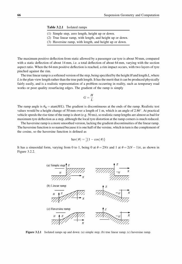
The maximum positive deflection from static allowed by a passenger car tyre is about 50mm, compared

with a static deflection of about 14mm, i.e. a total deflection of about 64mm, varying with the section

aspect ratio. When the 64mm positive deflection is reached, a rim impact occurs, with two layers of tyre

pinched against the rim.

The true linear ramp is a softened version of the step, being specifiedby the heightH and lengthL, where

L is the plan-view length rather than the true path length. It has themerit that it can be produced physically

fairly easily, and is a realistic representation of a problem occurring in reality, such as temporary road

works or poor quality resurfacing edges. The gradient of the ramp is simply

G ¼ H

L

The ramp angle is uR¼ atan(H/L). The gradient is discontinuous at the ends of the ramp. Realistic test

values would be a height change of 50mm over a length of 1 m, which is an angle of 2.86�. At practicalvehicle speeds the rise time of the ramp is short (e.g. 50ms), so realistic ramp lengths are almost as bad for

maximum tyre deflection as a step, although the local tyre distortion at the ramp corners is much reduced.

The haversine ramp is a more smoothed version, lacking the gradient discontinuities of the linear ramp.

The haversine function is so named because it is one half of the versine, which in turn is the complement of

the cosine, so the haversine function is defined as

havð uÞ ¼ 1

21� cosð uÞf g

It has a sinusoidal form, varying from 0 to 1, being 0 at u¼ 2Np and 1 at u¼ 2(N� 1)p, as shown in

Figure 3.2.2.

Figure 3.2.1 Isolated ramps up and down: (a) simple step; (b) true linear ramp; (c) haversine ramp.

Table 3.2.1 Isolated ramps

(1) Simple step, zero length, height up or down.

(2) True linear ramp, with length, and height up or down.

(3) Haversine ramp, with length, and height up or down.


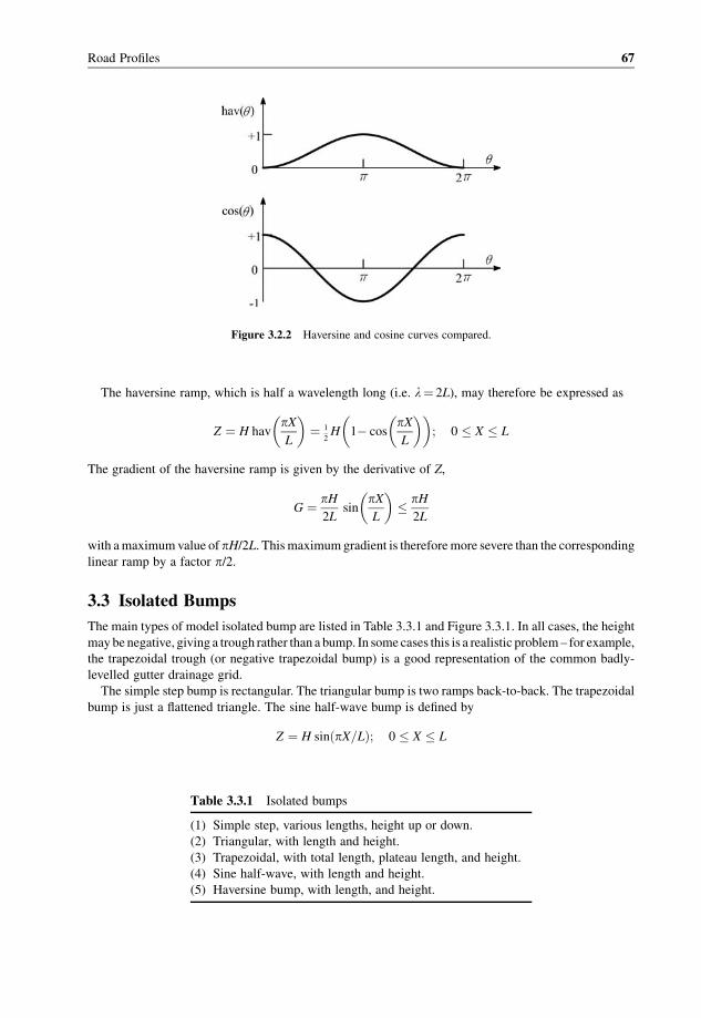
The haversine ramp, which is half a wavelength long (i.e. l¼ 2L), may therefore be expressed as

Z ¼ H havpXL

� �¼ 1

2H 1� cos

pXL

� �� ; 0 � X � L

The gradient of the haversine ramp is given by the derivative of Z,

G ¼ pH2L

sinpXL

� �� pH

2L

with amaximumvalue of pH/2L. Thismaximumgradient is thereforemore severe than the corresponding

linear ramp by a factor p/2.

3.3 Isolated Bumps

The main types of model isolated bump are listed in Table 3.3.1 and Figure 3.3.1. In all cases, the height

maybe negative, giving a trough rather than a bump. In some cases this is a realistic problem– for example,

the trapezoidal trough (or negative trapezoidal bump) is a good representation of the common badly-

levelled gutter drainage grid.

The simple step bump is rectangular. The triangular bump is two ramps back-to-back. The trapezoidal

bump is just a flattened triangle. The sine half-wave bump is defined by

Z ¼ H sinðpX=LÞ; 0 � X � L

Figure 3.2.2 Haversine and cosine curves compared.

Table 3.3.1 Isolated bumps

(1) Simple step, various lengths, height up or down.

(2) Triangular, with length and height.

(3) Trapezoidal, with total length, plateau length, and height.

(4) Sine half-wave, with length and height.

(5) Haversine bump, with length, and height.

Road Profiles 67

The gradient, by differentiation, is

G ¼ pHL

� �cos

pXL

� �

and is discontinuous at the ends. This is a typical shape used for a deliberately made traffic-slowing bump,

the ‘sleeping policeman’, with length from 1m to 3m.

The full haversine bump is defined by

Z ¼ H hav2pXL

� �; 0 � X � L

The gradient is

G ¼ pHL

� �sin

2pXL

� �

Figure 3.3.1 Isolated bumps and troughs up and down: (a) simple step; (b) triangular; (c) trapezoidal; (d) sine half-

wave; (e) haversine.


and is continuous, with a maximum value equal to that of the sine half-wave. (The sine wave actually has

twice the amplitude, but only one half is used.)

3.4 Sinusoidal Single Paths

In simple analytical ride studies the path or road is considered to have only one spatial frequency of

bumps at a time. This is known as a sinusoidal single-path road, Figure 3.4.1. All frequencies may be

considered, but only one at a time. It is also known in simulation studies as a single-track road, but this is

potentially confusing because in general motoring a single-track road is onewith the operating width of

a single vehicle.

Considering a sinusoidal road shape of wavelength lR, Figure 3.4.2, the spatial frequency of the roadnSR (cycles per metre, c/m) is

nSR ¼ 1

lRð3:4:1Þ

The radian spatial frequency of the road, vSR (rad/m), is

vSR ¼ 2pnSR ¼ 2plR

ð3:4:2Þ

At a vehicle longitudinal speed V, the observed frequency of road vibration stimulus is fR (Hz) with

corresponding radian frequency vR (rad/s) and period TR (in seconds):

TR ¼ lRV

ð3:4:3Þ

fR ¼ 1

TR¼ V

lR¼ VnSR ð3:4:4Þ

vR ¼ VvSR ð3:4:5Þ

Figure 3.4.1 Sinusoidal single paths of lower and higher spatial frequencies.

Road Profiles 69

It is therefore easy to find the vehicle speed or roadwavelengthwhichwill stimulate vehicle resonance at a

natural frequency fN:

V ¼ lfN ð3:4:6Þ

A heave or pitch resonance at 1.4Hz occurs for a wavelength of 10 m at a speed of 10� 1.4¼ 14m/s.

At a typical speed of 20m/s and fN¼ 1.4Hz the resonant wavelength is 14 m. A wheel hop resonance

at 10Hz will be stimulated at a speed of 20m/s by a wavelength of 20/10¼ 2.0m. At a wavelength of

0.1m, as found with cobblestones, wheel hop is stimulated at a speed of around 1m/s. A wavelength

of about 0.160m equals the tyre contact patch length, and stimulates longitudinal vibrations at the

wheel, independent of speed.

In Figure 3.4.2, when a purely sinusoidal road is being considered, the phase angle is normally zero.

However, when the sinusoids are the result of a Fourier analysis, the phase must be considered. In

general, for a given single wavelength lR and spatial radian frequency vSR there are sine and cosine

components, so

Z ¼ S sinðvSRXÞþCcosðvSRXÞ ð3:4:7Þ

These may be combined into a single sine wave of amplitude Z0 with a phase angle f:

Z ¼ Z0 sinðvSRXþfÞ ð3:4:8Þ

Expanding the sine double angle,

Z ¼ Z0fsinðvSRXÞcosfþ cosðvSRXÞsinfg ð3:4:9Þ

By comparison with equation 3.4.7,

S ¼ Z0 cosf

C ¼ Z0 sinf

so

Z0 ¼ffiffiffiffiffiffiffiffiffiffiffiffiffiffiffiS2 þC2

p

tanf ¼ C

S

as in Figure 3.4.3. The sine and cosine coefficientsmaybe of either sign, and the phase anglemust be found

in the correct quadrant (use Fortran Atan2(C,S) or Basic Angle(S,C). Note that the order of the arguments

differs).

Figure 3.4.2 Sinusoidal wavelength and phase angle.


3.5 Sinusoidal Roads

The sinusoidal road is essentially two sinusoidal paths, at a lateral spacing equal to the track (tread) of the

vehicle. This introduces several complications. The two sinusoidal paths may be symmetrical, anti-

symmetrical or arbitrary, corresponding to relative phase angles of zero, 180� or any value, Figure 3.5.1.Of course, this assumes that the two paths have sinusoids with the samewavelength, which is usual but not

actually physically essential.

When the two paths are in phase, then a symmetrical vehicle would respond symmetrically. However,

this simple case can be used to investigate the effect of vehicle asymmetries, such as different-length

steering track rods.

The purely antisymmetrical case, with 180 degrees of phase difference, stimulates the vehicle strongly

in roll. Again, this is a useful test of the effect of bump-steer and roll-steer geometry and of the steering

activity required to maintain a straight course.

In general, each path has its own phase angle,fL andfRleft and right, although the physical effect of the

phases on the vehicle depends only on the phase angle differencefL� fR. Each path may be expressed in

its sine and cosine components:

ZL ¼ SL sinðvSRXÞþCL cosðvSRXÞ

ZR ¼ SR sinðvSRXÞþCR cosðvSRXÞ

The road (viz. the pair of paths)maybe considered as a total symmetrical road partZS on the centreline plus

an antisymmetrical banking part ZB, half of the path height difference,

ZS ¼ 1

2ðZL þ ZRÞ

ZB ¼ 1

2ðZL � ZRÞ

and in reverse,

ZL ¼ ZS þ ZB

ZR ¼ ZS � ZB

The centreline road elevation is therefore

ZS ¼ 1

2ðSL þ SRÞ sinðvSRXÞþ 1

2ðCL þCRÞ cosðvSRXÞ

¼ SS sinðvSRXÞþCS cosðvSRXÞ

Figure 3.4.3 Sine component amplitude S, cosine component amplitude C, total amplitude Z0 and phase angle f.

Road Profiles 71

The banking component is

ZB ¼ 1

2ðSL � SRÞ sinðvSRXÞþ 1

2ðCL �CRÞcosðvSRXÞ

¼ SB sinðvSRXÞþCB cosðvSRXÞ

Figure 3.5.1 Sinusoidal two-track roads with various phase relationships: (a) in phase, symmetrical; (b) in antiphase,

antisymmetrical; (c) general.


The amplitudes are therefore related simply by

SS ¼ 1

2ðSL þ SRÞ

CS ¼ 1

2ðCL þ CRÞ

SB ¼ 1

2ðSL�SRÞ

CB ¼ 1

2ðCL�CRÞ

These may in turn be combined into total amplitudes and phases:

ZS ¼ ZS0 sinðvSRXþfSÞZB ¼ ZB0 sinðvSRXþfBÞ

ZS0 ¼ffiffiffiffiffiffiffiffiffiffiffiffiffiffiffiffiS2S þC2

S

q

ZB0 ¼ffiffiffiffiffiffiffiffiffiffiffiffiffiffiffiffiS2B þC2

B

q

The phase angles are

tan fS ¼ CS=SS; fS ¼ atan2ðCS; SSÞ

tan fB ¼ CB=SB; fB ¼ atan2ðCB; SBÞ

The antisymmetrical part may be considered to be due to a road bank angle fRB:

tan fRB ¼ 2ZB

T¼ ZL� ZR

T; �90� <fRB<90�

so

tan fRB ¼ 2

TfSB sinðvSRXÞþCB cosðvSRXÞg

¼ 2ZB0

TsinðvSRXþ fBÞ

The road bank angle is normally quite small, for passenger cars at least, in which case

fRB � tan fRB

Then the local road torsion is

kfRS � dfRB

dX¼ 2ZB0vSR

TcosðvSRXþ fBÞ

The total road torsion angle between the two axles of a vehicle ofwheelbaseL, with the rear axle at the path

position X, is

fRT ¼ fRB;XþL � fRB;X

Road Profiles 73

which is

fRT ¼ 2ZB0

TfsinðvSRðXþ LWÞþfBÞ � sinðvSRXþ fBÞg

3.6 Fixed Waveform

Some other waveforms are sometimes used in testing. A good example is the regularly-repeating

rectangular bump, as in Figure 3.6.1. This particular profile is characterised by the wavelength l, andthe rectangular bump length LB and height HB. The advantage of this particular path profile is that it is

easily constructed by laying down planks ofwood on an otherwise level surface. This profile has been used

to investigate the effect of profile roughness on the maximum cornering ability of cars, Figure 3.6.2, by

driving at near to the limit of cornering ability on a smooth entry section before entering the rough section.

The bumps may also be angled to the expected trajectory of the vehicle to introduce an asymmetrical

stimulus.

Figure 3.6.1 Path profile with repeating rectangular bump.

Figure 3.6.2 Rectangular-roughness cornering test.


3.7 Fourier Analysis

Fourier analysis was introduced by French mathematician Jean Baptiste Joseph Fourier (1768–1830) in

the context of thermodynamic analysis. (Simultaneously he explicitly introduced the idea that a scientific

equationmust have consistent units, launching the field of dimensional analysis.) The basic idea of Fourier

analysis is that any perfectly repetitive waveform can be represented exactly by the sum of many

sinusoidal waves. In Fourier’s day this was all done analytically, and in general an infinite number of

waves are required for an exact representation, with some lesser number giving an approximation. With a

digital representation of a waveform, the resolution is not perfect, and a finite number of sinusoidal waves

is sufficient for the perfect representation of the digital wave as sampled. A lesser number than that may

still be used if desired, provided that the approximation is acceptable.

Appendix F gives more information on the Fourier transform. For efficient digital calculation the fast

Fourier transform (FFT) is used, or specifically the digital Fourier transform (DFT), with a number of

points equal to 2MwhereM is an integer, for example 1024¼ 210 points equally spaced at typically 1 m or

one quarter of the wheelbase. The DFT then gives 512 frequencies each with one sine coefficient and one

cosine coefficient, for a total of 1024 coefficients (approximately, see Appendix F). This requires, in

principle, the solution of 1024 simultaneous equations for 1024 coefficients, but fortunately these are

decoupled and can be solved independently and therefore efficiently.

Applying the definitive ‘slow’ Fourier transform, the cosine and sine coefficients for frequency number

K are given respectively by

CK ¼ 2

N

XNJ¼1

YðJÞ cos�2pJKN

�; K ¼ 0; 1; . . . ;N=2

SK ¼ 2

N

XNJ¼1

YðJÞ sin�2pJKN

�; K ¼ 1; 2; . . . ;N=2�1

where thewavelength of that spatial frequency isL/K,Lbeing the physical length of the sample, not seen in

the above equations. The DFT solves for K¼ 1 to N/2.

The road profile (e.g. the original 1024 road heights) is recovered from the sine and cosine coefficients

for the Jth point by

ZðJÞ ¼ 1

2A0 þ

XM�1

K¼1

CK cos2pJKN

� �þ SK sin

2pJKN

� �� þ 1

2AM cos ðpJÞ

From the above equations, it is apparent that the mean value of the road height can have no effect on the

sine or cosine coefficients because they are always complete waves and contribute nothing to the mean

value. The mean is therefore accounted for separately:

Zm ¼ 1

N

XNK¼1

ZK

Amore difficult problem is that of the trend of the data. In the specific case of a road, there is generally a

gradient from one end of the data set to the other. The important point to appreciate is that a Fourier

transform is a transform of a repeated waveform. If path heights at points 1 to 1024 are specified, then the

heights of points 1025 onwards are, in the transform, the same as those for point 1 onwards. Therefore, to

do a Fourier transform it is implied in the dataset that ZNþK¼ ZK, although this is not explicitly in the data.

Considering a perfectly smooth road, butwith a gradient, so thatZN> Z1, the Fourier transform assumes

that ZNþ 1¼ Z1, and the transformwill be that of a sawtooth path with a sharp step down from ZN to ZNþ 1.

Road Profiles 75

Therefore the gradient must be removed. To do this, do not set ZN¼ Z1. The point ZNþ1 should be

measured to give the gradient explicitly. The degradiented data Z is then derived from the raw data H by

ZK ¼ HK � K � 1

NðHNþ1 �H1Þ

as in Figure 3.7.1.

Degradienting is part of a broader process of detrending, ideally removing the effects of all wavelengths

greater than the sample. For example, the road actually has significant amplitude content at twice the

Figure 3.7.1 Degradienting the raw road data.

Figure 3.7.2 Illustration of the accumulation of sine components of successive frequencies, showing the first few

frequencies only.


sample length, so there will be a consequent curvature in the sample, which will falsely appear as

frequency content in the Fourier analysis – so-called aliasing. This frequency content really is present in

the assumed repeatedwaveform, but not desired because it is not present in the real roadwhich is not really

an exact repeat of the sample. The Fourier analysis gives the correct frequency content of an infinite repeat

of the sample, rather than of the actual road. Failure to detrend the road data will result in considerable

spurious frequency content, particularly at high frequencies, with bad results.

When a simulated road is reconstructed from a set of sine and cosine coefficients, then the waveform

produced is, naturally, a repeating one outside its basic length.

Anti-aliasing and ‘degradienting’ is really an area for specialists – vehicle dynamicists can mostly just

use the results, such as the ISO standard road spectrum, which encapsulates the characteristics of roads as

revealed by Fourier analysis, as discussed in a later section.

Figure 3.7.2 illustrates how a road profile being constructed by an inverse Fourier transform is

accumulated from successive frequencies.

3.8 Road Wavelengths

The spectral analysis of roads may be used to separate out the wavelengths into various categories

according to their effect, as in Table 3.8.1. At the short wavelengths, affecting tyre friction, the practical

division is intomacrostructure andmicrostructure, as seen in Figure 3.8.1. The range of wavelengths from

10mm to 100m, covering undulations and roughness, is the main area of interest for Fourier analysis in

ride quality studies.

3.9 Stochastic Roads

Real roads, subject to Fourier analysis, are found to have a spectral distribution of roughness declining

rapidly with spatial frequency, Figure 3.9.1 giving two examples. A commonly used road model has

Table 3.8.1 Road spectral analysis

Characteristic Wavelength Influence on

Slopes 100m< l Static

Undulations 1m< l< 100m Dynamic ride

Roughness 10mm< l< 1m Dynamic NVH (noise, vibration and harshness)

Macrotexture 1mm< l< 10mm Friction and noise

Microtexture 10mm< l< 1mm Friction

Material molecular Friction

Figure 3.8.1 Road surface macrostructure and microstructure.

Road Profiles 77

been that in Figure 3.9.2, with amplitude squared spectral density (so-called power spectral density,

PSD)

S ¼ SrefnS

nS;ref

� ��W

with the negative gradientW usually equal to 2.5 or 2.7. More complex models are also used with two

gradients, and various cut-off methods, and sometimes continuous curves.

If themaximum gradient of a sinusoid is constant, then the amplitude is proportional to thewavelength.

Then the amplitude squared (the spectral ‘power’) is proportional to the wavelength squared, and the

negative gradientWwould take the value 2. Therefore, for representative roads, withW> 2, themaximum

sinusoidal gradient reduces with frequency.

The ISO road surfacemodel has two linear sections as in Figure 3.9.3, with an average road specified by

a break point or reference point at a spatial frequency of 1 rad/m, which is a wavelength of 2pmetres. In

Figure 3.9.1 The spectral analysis of two example roads (spectral density versus spatial frequency).

Figure 3.9.2 The basic single gradient spectral model of a representative road surface.


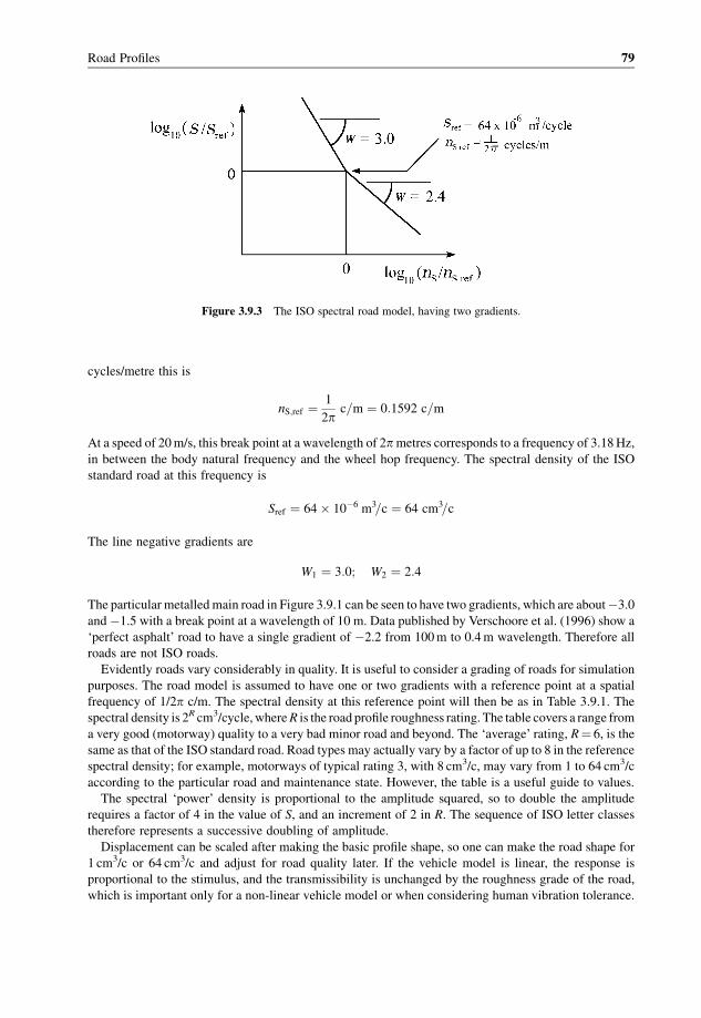
cycles/metre this is

nS;ref ¼ 1

2pc=m ¼ 0:1592 c=m

At a speed of 20m/s, this break point at a wavelength of 2pmetres corresponds to a frequency of 3.18Hz,

in between the body natural frequency and the wheel hop frequency. The spectral density of the ISO

standard road at this frequency is

Sref ¼ 64� 10�6 m3=c ¼ 64 cm3=c

The line negative gradients are

W1 ¼ 3:0; W2 ¼ 2:4

The particular metalledmain road in Figure 3.9.1 can be seen to have two gradients, which are about�3.0

and�1.5 with a break point at a wavelength of 10 m. Data published by Verschoore et al. (1996) show a

‘perfect asphalt’ road to have a single gradient of �2.2 from 100m to 0.4m wavelength. Therefore all

roads are not ISO roads.

Evidently roads vary considerably in quality. It is useful to consider a grading of roads for simulation

purposes. The road model is assumed to have one or two gradients with a reference point at a spatial

frequency of 1/2p c/m. The spectral density at this reference point will then be as in Table 3.9.1. The

spectral density is 2R cm3/cycle,whereR is the road profile roughness rating. The table covers a range from

a very good (motorway) quality to a very bad minor road and beyond. The ‘average’ rating, R¼ 6, is the

same as that of the ISO standard road. Road types may actually vary by a factor of up to 8 in the reference

spectral density; for example, motorways of typical rating 3, with 8 cm3/c, may vary from 1 to 64 cm3/c

according to the particular road and maintenance state. However, the table is a useful guide to values.

The spectral ‘power’ density is proportional to the amplitude squared, so to double the amplitude

requires a factor of 4 in the value of S, and an increment of 2 in R. The sequence of ISO letter classes

therefore represents a successive doubling of amplitude.

Displacement can be scaled after making the basic profile shape, so one can make the road shape for

1 cm3/c or 64 cm3/c and adjust for road quality later. If the vehicle model is linear, the response is

proportional to the stimulus, and the transmissibility is unchanged by the roughness grade of the road,

which is important only for a non-linear vehicle model or when considering human vibration tolerance.

Figure 3.9.3 The ISO spectral road model, having two gradients.

Road Profiles 79

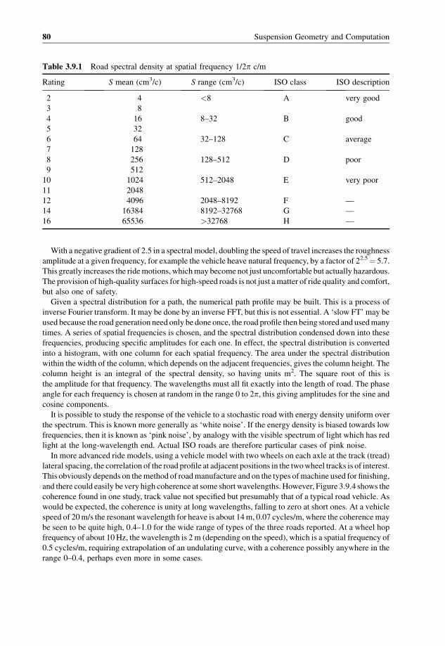
With a negative gradient of 2.5 in a spectral model, doubling the speed of travel increases the roughness

amplitude at a given frequency, for example the vehicle heave natural frequency, by a factor of 22.5¼ 5.7.

This greatly increases the ridemotions,whichmay become not just uncomfortable but actually hazardous.

The provision of high-quality surfaces for high-speed roads is not just amatter of ride quality and comfort,

but also one of safety.

Given a spectral distribution for a path, the numerical path profile may be built. This is a process of

inverse Fourier transform. It may be done by an inverse FFT, but this is not essential. A ‘slow FT’ may be

used because the road generation need only be done once, the road profile then being stored and usedmany

times. A series of spatial frequencies is chosen, and the spectral distribution condensed down into these

frequencies, producing specific amplitudes for each one. In effect, the spectral distribution is converted

into a histogram, with one column for each spatial frequency. The area under the spectral distribution

within the width of the column, which depends on the adjacent frequencies, gives the column height. The

column height is an integral of the spectral density, so having units m2. The square root of this is

the amplitude for that frequency. The wavelengths must all fit exactly into the length of road. The phase

angle for each frequency is chosen at random in the range 0 to 2p, this giving amplitudes for the sine and

cosine components.

It is possible to study the response of the vehicle to a stochastic road with energy density uniform over

the spectrum. This is known more generally as ‘white noise’. If the energy density is biased towards low

frequencies, then it is known as ‘pink noise’, by analogy with the visible spectrum of light which has red

light at the long-wavelength end. Actual ISO roads are therefore particular cases of pink noise.

In more advanced ride models, using a vehicle model with two wheels on each axle at the track (tread)

lateral spacing, the correlation of the road profile at adjacent positions in the twowheel tracks is of interest.

This obviously depends on themethod of roadmanufacture and on the types ofmachine used for finishing,

and there could easily be very high coherence at some short wavelengths. However, Figure 3.9.4 shows the

coherence found in one study, track value not specified but presumably that of a typical road vehicle. As

would be expected, the coherence is unity at long wavelengths, falling to zero at short ones. At a vehicle

speed of 20m/s the resonant wavelength for heave is about 14m, 0.07 cycles/m, where the coherencemay

be seen to be quite high, 0.4–1.0 for the wide range of types of the three roads reported. At a wheel hop

frequency of about 10Hz, thewavelength is 2 m (depending on the speed), which is a spatial frequency of

0.5 cycles/m, requiring extrapolation of an undulating curve, with a coherence possibly anywhere in the

range 0–0.4, perhaps even more in some cases.

Table 3.9.1 Road spectral density at spatial frequency 1/2p c/m

Rating S mean (cm3/c) S range (cm3/c) ISO class ISO description

2 4 <8 A very good

3 8

4 16 8–32 B good

5 32

6 64 32–128 C average

7 128

8 256 128–512 D poor

9 512

10 1024 512–2048 E very poor

11 2048

12 4096 2048–8192 F —

14 16384 8192–32768 G —

16 65536 >32768 H —


The real road is manufactured in a highly directional manner, so there is little reason, a priori, to expect

the road to be isotropic (properties independent of direction), and in some cases clearly it is not. For

example, in soft groundwhen there are ruts from the passage of thewheels the transverse section has a very

strong spectral density at a particular wavelength. Studies of metalled roads do indicate lack of isotropy,

but in a highly unsystematic way, so isotropy may still be a reasonable way to anticipate the relationship

between adjacent tracks.When there are no actual data, and a road of two ormore tracks is to be generated,

isotropy is the logical assumption. Figure 3.9.5 shows the coherence between tracks calculated on this

basis.

A numerical road of two adjacent tracks is then to be created from a spectral density and a coherence

graph. For each spatial frequency in turn, one track ismade as for a single track. For a real road, analysis of

0.1 0.2 0.3

Frequency [cycl/m]

A Pavement road

B Asphalt road

C Perfect asphaltA B C

Coher

ence

funct

ion

0.4

1

0.8

0.6

0.4

0.2

0

Figure 3.9.4 Coherence between two adjacent tracks (Verschoore et al., (1996). Reproduced with permission from:

Verschoore, Duquesne and Kermis (1996) ‘Determination of the vibration comfort of vehicles by means of simulation

and maeasurement’, EJME 41(3), pp. 137–143.

Figure 3.9.5 Coherence between adjacent tracks, on the assumption of a spectral density withW¼ 2.5 and isotropy.

The track spacing is 2b. Reproduced with permission from: J. D. Robson (1979) ‘Road surface description and vehicle

response’, IJVD 1(1), pp. 25–35. � Inderscience.

Road Profiles 81

the second path would show a slightly different amplitude, but for the simulated road it is usual, and

reasonable, to use the same amplitude for the two tracks. The second track is therefore usually given the

same amplitude as the first. The phase difference between the tracks depends on the coherence for that

wavelength. However, the coherence is not explicit, and is only a guide to the range of randomness, and

actually the distribution is not specified, only the effective mean. For a given wavelength and coherence

from the graph, the phase difference f may be taken with reasonable realism as

f ¼ � pð1�CPÞRand

with equal probability for either sign, where CP is the coherence between the paths and Rand is a 0–1

random deviate. Alternatively one can use a phase difference of

f ¼ �2pnST Rand

or

f ¼ pnSTf2ðRandþRandþRandÞg

where it should be noted that the sum of three independent Rand calls is not the same as 3�Rand.

References

Robson J. D. (1979) Road surface description and vehicle response. International Journal of Vehicle Design, 1(1),

25–35.

Verschoore, R., Duquesne, F. and Kermis, L. (1996) Determination of the vibration comfort of vehicles by means of

simulation and measurement. European Journal of Mechnical Engineering, 41(3), 137–143.

————— // —————


4

Ride Geometry

4.1 Introduction

Ride and handling motions of the body are the results of road roughness and control inputs, and are

associated with movement of the suspension. Therefore, it is necessary to specify various aspects of the

position and shape of the vehicle body, suspension and tyres. Thismay be done in a general way applicable

to all forms of suspensions, in terms of suspension bump position, body ride heights, etc. The vehicle

body ride position is specified by its heave, pitch and roll values. When the car is in combined braking

and cornering, the consequent heave, pitch and roll result in a different suspension bump at each wheel.

Bump is upward displacement of a wheel relative to the car body. Droop is negative bump. Heave is

symmetrical upward displacement of the body, or of an axle, then often called double bump. These are

special cases of the general terminolgy of vehicle positions and velocities, surge (X), sway (Y), heave (Z),

yaw (about the vertical axis), pitch (about the lateral horizontal axis) and roll (about the vehicle

longitudinal axis).

Bump and body heave influence the wheel camber and steer angles relative to the body and road, and

also influence the spring and damper forces and hence the tyre vertical force. These all influence the tyre

lateral force. The terms ‘bump’ and ‘droop’ may also be applied to velocities to show the direction of

motion; in that case it should be borne inmind that a bump velocitymay occur in a droop position, and vice

versa. Bump velocities also affect the slip angle because of the scrub velocity component. Body roll in

cornering gives a combination of bump and droop on opposite wheels, relative to the body.

Figure 4.1.1 shows an assortment of tyres with widely varying tread patterns for various applications.

For a given vehicle, the best wheel/tyre width and tread form depend on the road material (tarmac, mud,

snow, surface water, etc.) and surface shape (roughness, etc.).

4.2 Wheel and Tyre Geometry

Tyre geometry can be an extremely complex subject, particularly for the analysis of carcase reinforce-

ment, which will not be discussed here; this section covers only basic wheel and tyre deflection geometry

and terminology. Figure 4.2.1 gives the basic dimensional definitions. Contact patch shapes are generally

somewhat more elliptical in shape. The gross contact patch area is the area within the outer non-concave

profile. The net area is the area of rubber deemed to be actually in contact with the road, about 75% of the

gross area for a normal tyre. The contact patch solidity is the net area over the gross area, and is high for

best grip in dry conditions, but low for good water drainage. At a finer scale, of course, even the net area

is only partially in actual contact, with the rubber draping over the fine road asperities.


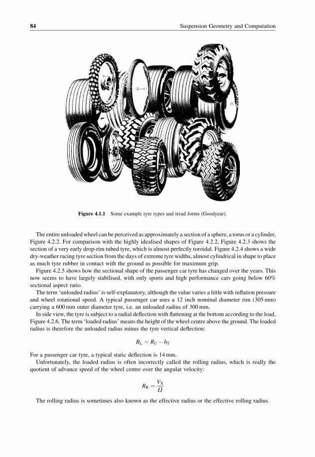
The entire unloadedwheel can be perceived as approximately a section of a sphere, a torus or a cylinder,

Figure 4.2.2. For comparison with the highly idealised shapes of Figure 4.2.2, Figure 4.2.3 shows the

section of a very early drop-rim tubed tyre, which is almost perfectly toroidal. Figure 4.2.4 shows a wide

dry-weather racing tyre section from the days of extreme tyre widths, almost cylindrical in shape to place

as much tyre rubber in contact with the ground as possible for maximum grip.

Figure 4.2.5 shows how the sectional shape of the passenger car tyre has changed over the years. This

now seems to have largely stabilised, with only sports and high performance cars going below 60%

sectional aspect ratio.

The term ‘unloaded radius’ is self-explanatory, although the value varies a little with inflation pressure

and wheel rotational speed. A typical passenger car uses a 12 inch nominal diameter rim (305mm)

carrying a 600mm outer diameter tyre, i.e. an unloaded radius of 300mm.

In side view, the tyre is subject to a radial deflection with flattening at the bottom according to the load,

Figure 4.2.6. The term ‘loaded radius’ means the height of thewheel centre above the ground. The loaded

radius is therefore the unloaded radius minus the tyre vertical deflection:

RL ¼ RU � hT

For a passenger car tyre, a typical static deflection is 14mm.

Unfortunately, the loaded radius is often incorrectly called the rolling radius, which is really the

quotient of advance speed of the wheel centre over the angular velocity:

RR ¼ VX

V

The rolling radius is sometimes also known as the effective radius or the effective rolling radius.

Figure 4.1.1 Some example tyre types and tread forms (Goodyear).


By simple geometric analysis of Figure 4.2.6, the angle subtended at the wheel centre by the contact

patch is

uCP ¼ 2 acosRL

RU

� �¼ 2 acos 1� hT

RU

� �

Typically, this is about 35�. The length of the contact patch is

LCP ¼ 2RU sin uCP �ffiffiffiffiffiffiffiffiffiffiffiffiffi8RUhT

pTypically this gives about 180mm, in agreement with direct measurement.

Figure 4.2.1 Tyre and rim leading dimensions.

Figure 4.2.2 Basic wheel shapes in front view: (a) spherical; (b) toriodal; (c) cylindrical.

Ride Geometry 85

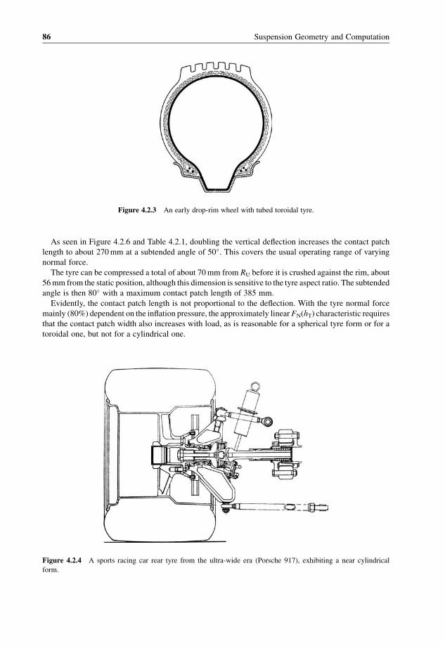
As seen in Figure 4.2.6 and Table 4.2.1, doubling the vertical deflection increases the contact patch

length to about 270mm at a subtended angle of 50�. This covers the usual operating range of varying

normal force.

The tyre can be compressed a total of about 70mm from RU before it is crushed against the rim, about

56mm from the static position, although this dimension is sensitive to the tyre aspect ratio. The subtended

angle is then 80� with a maximum contact patch length of 385 mm.

Evidently, the contact patch length is not proportional to the deflection. With the tyre normal force

mainly (80%) dependent on the inflation pressure, the approximately linearFN(hT) characteristic requires

that the contact patch width also increases with load, as is reasonable for a spherical tyre form or for a

toroidal one, but not for a cylindrical one.

Figure 4.2.3 An early drop-rim wheel with tubed toroidal tyre.

Figure 4.2.4 A sports racing car rear tyre from the ultra-wide era (Porsche 917), exhibiting a near cylindrical

form.


Where the rolling tyre arrives at and leaves the ground, at the ends of the contact patch, the tread

makes a turn through an angle of u/2. Figure 4.2.7(a) shows the simplified geometry, whilst Figure 4.2.7(b)

shows how the idealised tread curvature varies with position, the real graph being somewhat rounded,

of course. When the wheel is rolling, at entry to the contact patch the tread is sharply bent into a small

radius, and then promptly flattened out to zero curvature. At the rear of the contact patch, the tread is

sharply bent and then promptly reverts to the unloaded radius. This severe multiple flexing of the tread

is a large factor in the tyre rolling resistance.

Figure 4.2.6 Idealised tyre deflection geometry.

Figure 4.2.5 The progressive development of cross-sectional geometry (profile aspect ratio) of passenger car tyres

(Continental).

Table 4.2.1 Tyre compression geometry (passenger car tyre, RU¼ 300mm)

Condition hT (mm) RL (mm) u (deg) LCP (mm)

Static 14 286 35 181

Double 28 272 50 253

Limit 56 244 80 385

Ride Geometry 87

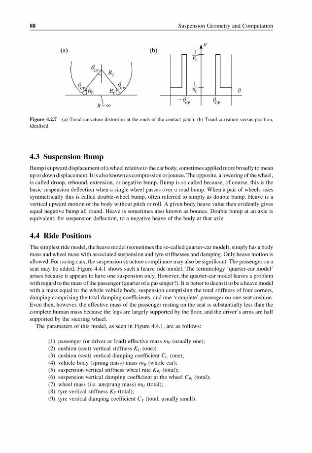
4.3 Suspension Bump

Bump is upward displacement of awheel relative to the car body, sometimes appliedmore broadly tomean

up or downdisplacement. It is also known as compression or jounce. The opposite, a lowering of thewheel,

is called droop, rebound, extension, or negative bump. Bump is so called because, of course, this is the

basic suspension deflection when a single wheel passes over a road bump. When a pair of wheels rises

symmetrically this is called double-wheel bump, often referred to simply as double bump. Heave is a

vertical upward motion of the body without pitch or roll. A given body heave value then evidently gives

equal negative bump all round. Heave is sometimes also known as bounce. Double bump at an axle is

equivalent, for suspension deflection, to a negative heave of the body at that axle.

4.4 Ride Positions

The simplest ridemodel, the heavemodel (sometimes the so-called quarter-car model), simply has a body

mass and wheel mass with associated suspension and tyre stiffnesses and damping. Only heave motion is

allowed. For racing cars, the suspension structure compliance may also be significant. The passenger on a

seat may be added. Figure 4.4.1 shows such a heave ride model. The terminology ‘quarter-car model’

arises because it appears to have one suspension only. However, the quarter-car model leaves a problem

with regard to themass of the passenger (quarter of a passenger?). It is better to deem it to be a heavemodel

with a mass equal to the whole vehicle body, suspension comprising the total stiffness of four corners,

damping comprising the total damping coefficients, and one ‘complete’ passenger on one seat cushion.

Even then, however, the effective mass of the passenger resting on the seat is substantially less than the

complete human mass because the legs are largely supported by the floor, and the driver’s arms are half

supported by the steering wheel.

The parameters of this model, as seen in Figure 4.4.1, are as follows:

(1) passenger (or driver or load) effective mass mP (usually one);

(2) cushion (seat) vertical stiffness KC (one);

(3) cushion (seat) vertical damping coefficient CC (one);

(4) vehicle body (sprung mass) mass mB (whole car);

(5) suspension vertical stiffness wheel rate KW (total);

(6) suspension vertical damping coefficient at the wheel CW (total);

(7) wheel mass (i.e. unsprung mass) mU (total);

(8) tyre vertical stiffness KT (total);

(9) tyre vertical damping coefficient CT (total, usually small).

Figure 4.2.7 (a) Tread curvature distortion at the ends of the contact patch. (b) Tread curvature versus position,

idealised.


Geometrically, measured from the datum level at Z¼ 0, there are the following vertical positions

of defining points on the masses:

(1) road height (from ‘roughness’) ZR;

(2) wheel centre height ZW;

(3) body ride height ZB;

(4) passenger ride height ZP.

The variations of these from the static values are the ride displacements, for example

zB ¼ ZB � ZB0

and are as follows:

(1) passenger ride displacement zP;

(2) body ride displacement zB;

(3) wheel ride displacement zW.

There are also:

(1) tyre ride deflection zT¼ zR� zW;

(2) suspension ride deflection (bump) zS¼ zW� zB;

(3) cushion (seat) ride deflection zC¼ zB� zP.

Expressing the above displacement equations in a summation form,

zR ¼ zT þ zW

zW ¼ zS þ zB

zB ¼ zC þ zP

Figure 4.4.1 Heave ride model including passenger, defining inertia, stiffness and damping coefficient notation and

ride positions.

Ride Geometry 89

The ride displacement of the road can therefore be expressed in three simple ways:

zR ¼ zT þ zW

zR ¼ zT þ zS þ zB

zR ¼ zT þ zS þ zC þ zP

4.5 Pitch

Pitch is the angle of the body in rotation about a transverse axis (i.e. nose up and nose down), and is

associated with braking and acceleration transients and response to road roughness. Relative to the static

position, the body pitch angle is uB, often considered positive with the nose up. This is a positive right-

hand rotation about a transverse vehicle-fixed axis to the right, as in the Society of Automotive Engineers

(SAE) axis system. However, in the ISO system, the transverse (Y ) axis is to the left, so arguably positive

pitch angle should then be positive nose-down. It is not essential to follow the right-hand rule for

rotations, although in dynamic analysis it is safer to do so. However, the signs can easily be adjusted.

In the application of equations, care is requiredwith this sign convention, which will be that positive pitch

is nose up.

In combinationwith the road elevations at the axles, the body pitch angle requires ride deflections at the

axles, accounted for mainly by the suspension, and partly by tyre deflections.

4.6 Roll

Body roll is rotation about the body longitudinal axis, arising from cornering activity and road roughness.

In both SAE and ISO systems, the longitudinal axis is forwards, so roll angle is positive for rotations

clockwise seen from the rear, i.e. body down on the right-hand side, as in a left-hand turn. Suspension roll

is formally defined (SAE) as rotation of the vehicle sprung mass about a fore–aft axis with respect to a

transverse line joining a pair of wheel centres. This is unambiguous provided that the ground is flat and

that front and rear wheel centres have parallel transverse lines (e.g. that wheels and tyres are the same size

side-to-side). If the ground is not flat then some mean ground plane must be adopted. The roll angle and

roll velocity are in practice fairly clear concepts. Asymmetries, such as the driver, mean that the roll

angle is not automatically zero under reference conditions, although it is usual practice to work in terms

of the roll relative to the static position.

Body roll is accommodated by suspension roll, plus some axle roll from tyre deflection, Figure 4.6.1.

On a level road (i.e. zero road bank angle)

fB ¼ fS þfA

For a passenger car, the axle roll is generally fairly small compared with the suspension roll, but this is

certainly not true for many racing cars with stiff suspensions, where inclusion of the axle roll angles is

essential.

For a torsionally-rigid vehicle body, in relation to the torsionalmoments applied, the body torsion angle

fBT is negligible. This is applicable to most passenger cars, in which case

fBT ¼ 0

fBf ¼ fBr

fBf ¼ fSf þ fAf

fBr ¼ fSr þ fAr


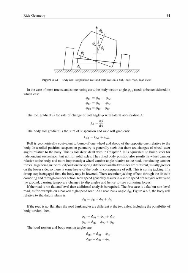
In the case of most trucks, and some racing cars, the body torsion angle fBT needs to be considered, in

which casefBf ¼ fSf þ fAf

fBr ¼ fSr þ fAr

fBT ¼ fBf �fBr

The roll gradient is the rate of change of roll angle f with lateral acceleration A:

kf ¼ df

dA

The body roll gradient is the sum of suspension and axle roll gradients:

kBf ¼ kSf þ kAf

Roll is geometrically equivalent to bump of one wheel and droop of the opposite one, relative to the

body. In a rolled position, suspension geometry is generally such that there are changes of wheel steer

angles relative to the body. This is roll steer, dealt with in Chapter 5. It is equivalent to bump steer for

independent suspension, but not for solid axles. The rolled body position also results in wheel camber

relative to the body, and more importantly a wheel camber angle relative to the road, introducing camber

forces. In general, in the rolled position the spring stiffnesses on the two sides are different, usually greater

on the lower side, so there is some heave of the body in consequence of roll. This is spring jacking. If a

droop stop is engaged first, the body may be lowered. There are other jacking effects through the links in

cornering and through damper action. Roll speed generally results in a scrub speed of the tyres relative to

the ground, causing temporary changes to slip angles and hence to tyre cornering forces.

If the road is not flat and level then additional analysis is required. The first case is a flat but non-level

road, as for example on a banked high-speed road. At a road bank angle fR, Figure 4.6.2, the body roll

relative to the datum plane isfB ¼ fR þ fA þ fS

If the road is not flat, then the road bank angles are different at the two axles. Including the possibility of

body torsion, then,

fBf ¼ fRf þ fAf þ fSf

fBr ¼ fRr þ fAr þ fSr

The road torsion and body torsion angles are

fRT ¼ fRf � fRr

fBT ¼ fBf � fBr

Figure 4.6.1 Body roll, suspension roll and axle roll on a flat, level road, rear view.

Ride Geometry 91

4.7 Ride Height

Ride height is the position of the body (sprung mass) above the basic ground level datum plane. The

dynamic ride height is the ride height relative to the static position. In general, during acceleration, braking

or cornering and on rough roads, the ride heights vary continuously and have different values at each

wheel. The set-up of the vehicle on an accurate level surface is the static ride height, in practice frequently

referred to simply as ride height. Values are specified for the front and rear of the vehicle. Normally it is

assumed that the vehicle should have zero body roll in the static position, although some static roll may be

specified in special cases, such as racing vehicles on tracks with turns predominantly in one direction.

The front and rear ride heights may be specified at any points that are convenient for measurement.

Hence particular points on the front and rear bodywork may be used. However, from the point of view of

vehicle dynamics, it is the ride heights at the wheels that are of importance. Hence, for passenger cars it is

convenient tomeasure the ride height at the highest point of thewheel arch opening, the so-called eyebrow

level. For ground-effect racing cars, the rules frequently specify a flat, or partially flat, underbody, inwhich

case this flat plane is often used to define the ride heights. Alternatively,measurementsmay bemade to the

inner axis of the bottom suspension arm.

Under running conditions, the ride heights or vertical positions of the body (sprung mass), of the wheel

and of the local road position aremeasured from a datum level, typically themean road plane. Figure 4.7.1

shows this for one suspension unit. Hence there are vertical positions ZB to some reference point on the

body, ZW to the wheel centre and ZR to the road height above datum. Each of these has four values, one at

each wheel specified by appropriate subscripts, normally either:

(1) f and r for front and rear, with L and R for left and right, or i and o for inner and outer.

(2) 1, . . ., 4 in the order

1: left front

2: right front

3: left rear

4: right rear

as in Figure 4.7.2.

Figure 4.6.2 Body roll, suspension roll and axle roll on a flat, non-level road, rear view.


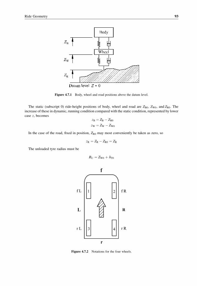
The static (subscript 0) ride-height positions of body, wheel and road are ZB0; ZW0; and ZR0. Theincrease of these in dynamic, running condition compared with the static condition, represented by lower

case z, becomeszB ¼ ZB � ZB0

zW ¼ ZW � ZW0

In the case of the road, fixed in position, ZR0 may most conveniently be taken as zero, so

zR ¼ ZR � ZR0 ¼ ZR

The unloaded tyre radius must be

RU ¼ ZW0 þ hT0

Figure 4.7.2 Notations for the four wheels.

Figure 4.7.1 Body, wheel and road positions above the datum level.

Ride Geometry 93

so the static tyre deflection is

hT0 ¼ RU � ZW0

The static loaded radius is

RL0 ¼ ZW0 ¼ RU � hT0

In running conditions, the loaded radius is

RL ¼ ZW � ZR

The running tyre deflection is

hT � RU � RL

which, however, cannot be negative. This becomes

hT ¼ hT0 � ZW þ ZR

The increase of tyre deflection zT is simply

zT ¼ zR � zW

Frequently in handling analysis, the road is deemed to be smooth and level, giving

zR ¼ 0

hT ¼ hT0 � zWzT ¼ � zW

The suspension bump deflection is

zS ¼ zW � zB

The basic body height is measured at the centre of mass, giving a single value for ZB. Incorporating the

body pitch angle uB (relative to static uB1), the body roll anglefB (the body not assumed torsionally rigid,

the static roll assumed to be zero) then changes the body height at the four wheels, that is, the body ride

heights are, with pitch angle sign convention positive nose-up,

zBfL ¼ zB þ a sin uB þ 1

2Tf sinfBf

zBfR ¼ zB þ a sin uB � 1

2Tf sinfBf

zBrL ¼ zB � b sin uB þ 1

2Tr sinfBr

zBrR ¼ zB � b sin uB � 1

2Tr sinfBr

where a and b are the front and rear partial wheelbases. The pitch and roll angles are generally moderately

small, with sin u� u, so it is common practice to use the computationally much more efficient

zBfL ¼ zB þ a uB þ 1

2Tf fBf

zBfR ¼ zB þ a uB � 1

2Tf fBf

zBrL ¼ zB � b uB þ 1

2Tr fBr

zBrR ¼ zB � b uB � 1

2Tr fBr


Normal practicewould be to precalculate the front and rear mean ride heights, and the half-track values

too of course, with

zBf ¼ zB þ a uB

zBr ¼ zB � b uB

zBfL ¼ zBf þ�1

2 Tf

�fBf

zBfR ¼ zBf ��1

2 Tf

�fBf

zBrL ¼ zBr þ�1

2 Tr

�fBr

zBrR ¼ zBr ��1

2 Tr

�fBr

There are similar expressions, but with some sign changes, for the small deflections of the unsprung

mass considered normally in terms of a pitch angle and front and rear roll angles. These are tyre, unsprung

mass or axle, pitch and roll angles and deflections. In practice they are usually called tyre deflections,

axle roll angles, and unsprung pitch angle.

The actual body ride positions are given by equations of the form

ZBfL ¼ ZBfL0 þ zBfL

With dynamic solution of the tyre deflections, and hence wheel heights, the suspension bump

deflections during running are then of the form

zSfL ¼ zWfL� zBfL

which is positive for bump (suspension compression).

Similar equations to the above apply for velocities. In a time-stepping computer simulation the

velocities will usually be obtained by integrating the acceleration over the time step, or possibly in some

cases from displacements divided by the time increment.

For any given body position (heave, pitch, roll) the four ride heights and ride velocities can be evaluated

as above. In a handling analysis, the frequency range considered will normally be below the wheel hop

frequency, so in steady-state handling the wheel will often be assumed to adopt an equilibrium height

according to the body ride height, the suspension stiffness and the tyre vertical stiffness. Hence the

position and velocities are determined, from which the suspension stiffness and damping forces and

tyre forces follow.

4.8 Time-Domain Ride Analysis

The road stimulus considered may be a simple sinusoid to investigate the vehicle behaviour at a

given frequency. This may also be done analytically, but with computer time-stepping it is feasible to

have non-linear components. In this case the resulting positions and displacements vary sinusoidally

(for linear components) or approximately sinusoidally (for non-linear) at the forcing frequency, and the

ratio of the response amplitude to the road amplitude gives a transmissibility to each of the wheel, body

and passenger for that frequency.

Alternatively, the simulated road may be given a white or pink noise characteristic, at least over a

frequency range of interest, say up to 15Hz; the response of each mass then has a semi-random nature

which can be statistically analysed.

Ride Geometry 95

With any stochastic road, there will be an overall root-mean-square (rms) displacement of the

suspension, which can be divided by the road rms displacement to give an rms transmissibility for these

conditions. Spectral analysis will also reveal certain resonances and responses; for example, there will be

an increased body response at the body resonant and wheel hop resonant frequencies.

A third option for the model road, frequently favoured, is to give the road a random nature based

statistically on the character of real roads, in which case the responses can be regarded as more realistic.

The random response of the bodies can then be analysed. The most important results are those for:

(1) the passenger rms response (for passenger comfort, i.e. ride),

(2) the tyre deflection rms variation (for tyre comfort, i.e. handling),

(3) the suspension rms displacement (for suspension comfort, i.e. workspace).

The assessment of passenger ride perception is called the ‘passenger discomfort’ DP. This is normally

defined as the rms acceleration experienced by the passenger, normalised by dividing by g, standard

gravity (ISO 9.80665m/s2, Imperial 32.174 ft/s2 or US 386 in/s2):

DP ¼ Arms

g

Multiplying by the passenger mass, it is seen that this is also equal to the rms variation of vertical force

supporting the passenger divided by the mean vertical force. Also, there is a direct geometrical

interpretation, For a linear cushion, it is the rms variation of cushion deflection over the mean value.

A ride simulation also gives a figure for the rms variation of tyre vertical force. The tyre discomfort is

DT ¼ ðDFVTÞrms

FVT;mean

Here FVT is the vertical force exerted by the road on the tyre. Hence the tyre discomfort is the rms value

of the vertical force fluctuations divided by themeanvertical force. Again, for a linear tyre there is a direct

geometrical interpretation: it is the rms variation of tyre deflection divided by the mean deflection.

The basic definition of passenger and tyre discomfort corresponds to the statistician’s coefficient of

variation, or the normalised standard deviation, the standard deviation divided by themean. The rms value

of a Gaussian distribution with zero mean is one standard deviation.

The suspension deflection or workspace can also be expressed in various ways as a suspension

discomfort.

4.9 Frequency-Domain Ride Analysis

Frequency-domain analysis considers the behaviour of the vehicle in terms of its response at any given

frequency of stimulus. Such analysis therefore produces results such as graphs of the transmissibility

against frequency.

For a simple linear system the behaviour at a given frequency may be obtained analytically. For more

complexmodels, or with non-linear components, it may be obtained by time-stepping analysis at each of a

series of frequencies of sinusoidal road profile or, more efficiently in general, by a broad spectrum

stimulus, using a road with some spectral distribution, with the response being spectrally analysed, the

transmissibility then being the amplitude ratio of response to stimulus, for each frequency of interest

through the spectrum.

The geometry of the stimulating road, then, may be sinusoidal, with various spatial frequencies taken in

turn, or stochastic, being either an actual road profile trace, or, more likely, a profile generated by inverse

Fourier transformfroma spectral densitydefinition such as the standard ISOroad, as discussed inChapter 3.


4.10 Workspace

The tyre, suspension and seat cushion are often analysed as simple linear components, but even then they

have a limited range of action. The tyrewill leave the ground at a negative dynamic deflection equal to the

static value. The suspension can hit the bump stops or droop stops, and the seat cushion will also have its

limits. These define the available workspace for each compliant component. The workspace in use is the

result of the dynamic response of the system to the road roughness. Typically the suspension bump

deflection will be analysed statistically to give a standard deviation of position for a given road.

The workspace requirement will then be considered to be about 3 standard deviations in each direction,

which will occasionally be exceeded. Similarly, the workspace requirement of the tyre and seat cushion

can be analysed. In practice, the suspension workspace requirement can be reduced by the use of a stiffer

spring, so there is a trade-off between the softness and comfort of the central action of the suspension

and more frequent limit impacts. A higher speed of travel increases the stimulus, because of the character

of the road spectrum, so high-speed vehicles need stiffer suspension for comfort, avoiding limit stop

impacts, not just for handling qualities.

With a typical passenger car static tyre deflection of 14mm, if the 3s workspace exceeds this value

then the tyre will leave the ground intermittently. This is a standard deviation of less than 5mm.

————— // —————

Ride Geometry 97

5

Vehicle Steering

5.1 Introduction

Directional control of a road vehicle is normally achieved by steering the front wheels, that is, by rotating

them about a roughly vertical axis. The effective steer rotation of thewheels relative to the body centreline

is represented by d (delta). This is mainly the result of steering handwheel movement by the driver, but

partly the result of suspension characteristics (bump steer, roll steer and compliance steer). Rear-wheel

steering is generally unsafe at high speeds, but because of its convenience in manoeuvring it is sometimes

used on specialist low-speed vehicles, such as dumper trucks. This is in contrast to aircraft, which usually

have tailplanes and are rear steered by elevators and rudder. Some interest has been shown in variable rear

steering for passenger cars, supplementing conventional front steering, and this is has been commercially

available.

In the early days of motoring, various hand controls were tried for the driver. Tiller steering, as used on

boats, for example as on the 1894 Panhard-Levassor in Figure 5.1.1, was satisfactory at low speed, but

often dangerously unstable at high speed. Thewheels steered in the same sense as the tiller, so the tillerwas

moved to the right tomake a left turn. The driver then tended to fall centrifugally to the right, exaggerating

the turn, sometimes leading to an unstable divergencewith disastrous roll-over. Tiller steering was greatly

improved by Lanchester who reversed its action to give better stability. It was Benz who introduced the

steering wheel, and this was almost universal by 1900. Tests in other control applications show that the

handwheel is the bestway to combine rapid largemovementswith fine precision. For cars, the roadwheels

steer through a total angle of about 70�, and the steering wheel through three and a half turns, requiring agear ratio of 18. The average is actually about 17 for power-assisted steering and 21 for unpowered

steering. For trucks the steering-wheel movement and gear ratio are about twice those for cars. A high

steering gear ratiomeans a smaller steering force at the handwheel rim, but a greater angularmovement is

needed.

The steering of the road wheels is not governed exclusively by the steering hand wheel position.

In addition there are:

(1) toe angle – the initial fixed settings;

(2) suspension geometric steer arising from vertical wheel motion coupled with the linkage

geometry, expressed through bump steer or roll steer;

(3) suspension compliance steer, resulting from forces or moments and link compliance, mainly

in the rubber bushes;

(4) steering system compliance, mainly arising from torsional compliance of the steering

column.


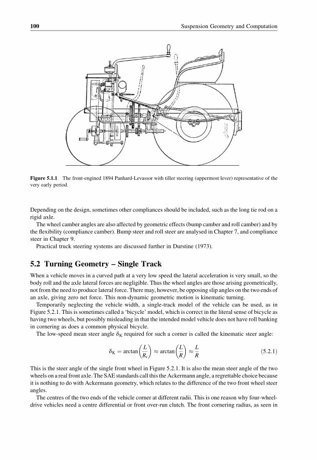
Depending on the design, sometimes other compliances should be included, such as the long tie rod on a

rigid axle.

Thewheel camber angles are also affected by geometric effects (bump camber and roll camber) and by

the flexibility (compliance camber). Bump steer and roll steer are analysed in Chapter 7, and compliance

steer in Chapter 9.

Practical truck steering systems are discussed further in Durstine (1973).

5.2 Turning Geometry – Single Track

When a vehicle moves in a curved path at a very low speed the lateral acceleration is very small, so the

body roll and the axle lateral forces are negligible. Thus the wheel angles are those arising geometrically,

not from the need to produce lateral force. Theremay, however, be opposing slip angles on the two ends of

an axle, giving zero net force. This non-dynamic geometric motion is kinematic turning.

Temporarily neglecting the vehicle width, a single-track model of the vehicle can be used, as in

Figure 5.2.1. This is sometimes called a ‘bicycle’ model, which is correct in the literal sense of bicycle as

having twowheels, but possibly misleading in that the intended model vehicle does not have roll banking

in cornering as does a common physical bicycle.

The low-speed mean steer angle dK required for such a corner is called the kinematic steer angle:

dK ¼ arctanL

Rr

� �� arctan

L

R

� �� L

Rð5:2:1Þ

This is the steer angle of the single front wheel in Figure 5.2.1. It is also the mean steer angle of the two

wheels on a real front axle. The SAE standards call this theAckermann angle, a regrettable choice because

it is nothing to do with Ackermann geometry, which relates to the difference of the two front wheel steer

angles.

The centres of the two ends of the vehicle corner at different radii. This is one reason why four-wheel-

drive vehicles need a centre differential or front over-run clutch. The front cornering radius, as seen in

Figure 5.1.1 The front-engined 1894 Panhard-Levassor with tiller steering (uppermost lever) representative of the

very early period.


Figure 5.2.1, is

Rf ¼ L

sin dKð5:2:2Þ

The rear cornering radius is

Rr ¼ L

tan dKð5:2:3Þ

Several other path radius values are also used. The SAEcornering radius is defined to be to the centre of the

outer front wheel. The clearance radius is the radius needed to clear the bodywork. In vehicle dynamic

analysis, the path radius of the centre of mass is the main one of interest.

The difference of the front and rear central radii is known as the offtracking. The offtracking radiusROT

is

ROT ¼ Rf � Rr ¼ L

sin d� L

tan dð5:2:4Þ

At low speed, with kinematic turning,

R2f ¼ R2

r þ L2 ð5:2:5Þ

Using

L2 ¼ R2f � R2

r ¼ ðRf þRrÞðRf � RrÞ ð5:2:6Þ

the offtracking can also be expressed as

ROT ¼ Rf � Rr ¼ L2

Rf þRr

� L2

2Rð5:2:7Þ

Figure 5.2.1 A single-track (upright bicycle) vehicle model, showing kinematic turning (low speed, no lateral forces,

zero tyre slip angles), turning centre CT.

Vehicle Steering 101

where R is the turn radius of the centre of mass. Example values for a passener car are L¼ 2.8m, d¼ 35�,Rr¼ 4m, Rf¼ 4.88m, ROT¼ 0.9m, so the offtracking can be quite large, leading to occasional kerbing of

the rear wheels which ‘cut the corner’. It is more problematic for long trucks, and especially for trailers.

The attitude angle b at a given point of the vehicle is the angle between the vehicle centreline and the

local velocity vector, which is perpendicular to the radial lines shown in Figure 5.2.2, in which it may be

seen that at low speed (negligible lateral acceleration, zero tyre slip angles) the attitude anglebr at the rear

axle is zero. Attitude angle is positive with the vehicle pointing towards the inside of the corner, so the

angles are negative in the figure. At the front axle

bf ¼ �arcsinL

R� � L

Rð5:2:8Þ

At the centre of mass, where the attitude angle is usually measured, the attitude angle is

b � � Lr

R¼ � Lr

LdK ð5:2:9Þ

Hence the attitude angle at the centre of mass takes a negative value under kinematic conditions; however,

it is positive-going as lateral acceleration develops, because of the increasing slip angle at the rear axle.

At significant speed, in dynamic cornering, tyre slip angles are required to produce thenecessarycornering

forces. Then attitude angle develops, and the offtracking also changes, Figure 5.2.3. The front and rear tyre

slip angles are denoted by af and ar, respectively. The angles are exaggerated in this figure for clarity of the

principle. Tyre slip angles are generally just a few degrees, not often exceeding 3� in everyday motoring.

Also, in normal cornering the path radius ismuch larger in relation to thewheelbase.The turning centre point

CT can be seen to havemoved forward from the rear axle line, or thevehicle can be considered tohave rotated

to a new attitude angle relative to the radius line from the turning centre. The attitude angles are then

br ¼ ar

b ¼ � Lr

Rþar

bf ¼ � L

Rþar

ð5:2:10Þ

Figure 5.2.2 Attitude angles at a given point of the vehicle depend on the local velocities, as seen here for kinematic

turning.


The condition of zero offtracking will occur when CT has moved forward half of the wheelbase. This

is possible for some particular speed depending on the cornering radius, according to tyre characteristics

etc., and occurs at typically 10m/s at 30m radius. At approximately the same speed, the attitude angle at

the centre ofmass becomes zero. For a greater speed, the offtracking becomes negative,with the rear of the

vehicle following a path of greater radius than the front.

5.3 Ackermann Factor

Consider now a vehicle with width, having axle track (tread). For a normal vehicle with front steering, to

turn with zero slip angles means that the turning centre CT must still be in line with the rear axle,

Figure 5.3.1. The front wheels must be steered by different amounts, the inner wheel more, in order

for both of them to have zero slip angle. Although actually invented by Darwin, Langensperger or others

(see Chapter 1), this is widely known as the Ackermann steering concept, and is desirable for low-speed

manoeuvring to avoid tyre scrub, minimising motion resistance, tyre wear and surface damage. Various

geometries are used in practice, more or less related to the basic Ackermann geometry.

For an axle, the difference between the steer angles of the two wheels to give zero or equal slip angles

equals the Langensperger angle l subtended at the turning centre by the axle. Positive Langensperger

angle iswith the axle turned out of the corner. In Figure 5.3.1, with kinematic turning,which has zeromean

tyre slip angles, evidently the Langensperger angle is positive for the front axle and zero for the rear axle.

For the front axle

lf0 ¼ � Tf sin bf

Rf

ð5:3:1Þ

where, kinematically, bf is negative and lf0 is positive. Substituting for the front attitude angle,

kinematically

lf0 ¼ �Tf � L

Rf

� �1

Rf

� Tf L

R2ð5:3:2Þ

Figure 5.2.3 Single-track model in dynamic turning, with front and rear tyre slip angles af and ar.


The basic front Langensperger angle is therefore simplyTL/R2, this giving the angle difference (in radians)

required for full Ackermann steering effect. The actual steer angle difference occurring in a given

condition, according to the actual steering mechanism geometry, is

dL�R ¼ dL� dR ð5:3:3Þ

For true Ackermann steering, then,

dL�R ¼ lf0 ð5:3:4Þ

for all steer angles, where lf0 is the Langensperger angle at zero lateral acceleration. The Ackermann

factor is then the ratio of the actual steer angle difference to the ideal difference:

fA ¼ dL�R

lf0ð5:3:5Þ

which is zero for parallel steering, and 1.0 (100%) for trueAckermann. For a real steering arrangement it is

only approximately a constant.

The difference between dL�R and l0 is sometimes called the tie-rod geometry error:

uTRGE ¼ dL�R � lf0 ¼ ðfA�1Þlf0 ð5:3:6ÞFor vehicles that do a great deal of turning or frequently need a very small turning radius, such as

purpose-built taxis and urban delivery vehicles, full Ackermann is often used. The Apollo ‘Lunar Rover’

vehicle had four-wheel steering, giving a minimum turn radius equal to the wheelbase of 2.286m, with

close to full Ackermann at both front and rear, tominimise resistance in tight turns on the soft ground. The

traditional London taxi has almost perfect Ackermann over its full 60� of inner road-wheel steer angle.

Figure 5.3.1 Turning geometry of a conventional passenger car at very low speed (negligible lateral acceleration).


There is less of a case for Ackermann steering geometry under dynamic cornering conditions. This is

because as attitude angle develops the Langensperger angle subtended by the front axle at the turning

centre reduces, Figure 5.3.2, and will go negative on fast large-radius corners. At the rear, the

Langensperger angle is always zero or negative. Also, because of lateral load transfer, the outer tyre

has greater vertical force, hence needing a greater slip angle than the inner tyre to produce its maximum

cornering force. Finally, roll steer effects may give a significant steer angle difference. Even anti-

Ackermann (negative fA) has been used on occasion. If the steering is not perfect Ackermann, then at low

speed each axle wheel pair must adopt equal and opposite slip angles to give zero net force.

Figure 5.3.3 shows the Ackermann geometry for a left turn. Here, the front ‘track’ T is measured

between the steer pivot axes at ground level – virtually the same as thewheel-centre track. Parallel lines are

Figure 5.3.3 Geometry for algebraic expression of the Ackermann condition.

Figure 5.3.2 Under dynamic cornering conditions, the axle Langensperger angles are changed, reducing or going

negative as attitude angle is introduced by lateral acceleration.


drawn from the pivots to the rear axle, these being RL and RR from the turn centre CT, as shown. The

algebraic expression for the Ackermann relationship is

cot dR � cot dL ¼ RR

L� RL

Lð5:3:7Þ

so for exact Ackermann effect

cot dR � cot dL ¼ T

Lð5:3:8Þ

This relationship can be expressed in an interesting geometric way, as in Figure 5.3.4 (see also

Heldt, 1948). A line is drawn from the centre of the front axle to the left rear axle point (for a left turn). The

steer angles, laid out as shown, should meet on this line. This can be proved as follows. In the diagram,

p cot dR � p cot dL ¼ 1

2T þ q

� �� 1

2T � q

� �¼ 2q ¼ 2

p

L

T

2so

cot dR � cot dL ¼ T

L

as required.

One convenient way to obtain complete or partial Ackermann steer angles is to angle the steering arms

inwards (for a rack or tie rod behind the kingpins), as in Figure 5.3.5, so that as steer is applied there is a

progressive difference in the effective moment arms of the steering arms. This slanting of the arms also

helpswithwheel and brake clearance. It iswidely believed that aligning the steering arms so that their lines

intersect at the rear axle will give true Ackermann steering (the Jeantaud diagram). However, this is far

from true, the actual Ackermann factor varying in a complex way with the arm angle, rack length, rack

offset forward or rearward of the arm ends, whether the rack is forward or rearward of the kingpins, and

with the actual mean steer angle. The Jeantaud arrangement with a single track rod and the steering arms

projected meeting at the rear axle actually gives about 60% of full Ackermann effect. To obtain an

Ackermann factor close to 1.0may require the projected steering arm intersection point to be at about 60%

of the distance to the rear axle.

Figure 5.3.4 Alternative geometric construction of the Ackermann condition.


Moving a steering rack forwards or backwards to change the track-rod angle relative to the steering arm

can be a useful way to obtain the desired Ackermann factor, the most important single variable being the

angle between the track rod and the steering arm in plan view, the Ackermann factor being proportional to

the deviation of this angle from 90�. Figure 5.3.6(a) shows the steering arm angle usually considered

important, as indeed it is with the aligned rack and track rods. Figure 5.3.6(b) shows the angle that is

actually important, the deviation from 90� at the steering arm to track rod joint. Figure 5.3.6(c) shows this

angle opened up bymoving the rack to the rear, increasing the Ackermann effect. Evidently, inclination of

the steering arms is not required at all, it can all be done by positioning the rack to give the necessary

included angle. With this method, forward steering arms need not be angled out, and can even be angled

inwards, as in Figure 5.3.6(d), although this increases the loads and wear on the rack.

As an interesting comparison, Figure 5.3.7 shows the La Mancelle/Benz type of mechanism, in which

the desired steering geometry is instead obtained by the triangular centre plate.

Considering the included angle between the track rod and the steering arm, with a conventional system,

as seen in Figure 5.3.6, denoting the deviation from 90� (p/2 rad) as the steering linkageAckermann effect

angle uStA, ideal (100%) Ackermann requires

uStA ¼ uStA;I � 1:6T

2L¼ 0:8

T

Lð5:3:9Þ

Figure 5.3.6 Ackermann effect achieved or altered by rack position.

Figure 5.3.5 BasicAckermann steeringmechanism, using a single tie rodwith steering arms inclined inwards, in plan

view. The section is at the height of the steering system, with the corresponding pivot axis point.


For a passenger car this is about 0.4 rad or 23�. The Ackermann factor is then

fA � uStAuStA;I

� 2:5 uStA ð5:3:10Þ

with the angle in radians.

5.4 Turning Geometry – Large Vehicles

Large vehicles basically fall into two categories: articulated and non-articulated. The latter are typified by

the (omni)bus. Here the vehicle length creates a manoeuvrability problem. A long wheelbasewith a given

steer angle gives a large turning radius and large offtracking. Therefore the wheelbase is typically made

shorter, with large body overhangs, Figure 5.4.1. Also, the steer angle is made larger than usual, possibly

50� as in Figure 5.4.2.

Figure 5.3.7 The La Mancelle/Benz type steering mechanism, using a triangular centre member to give the desired

Ackermann effect.

Figure 5.4.1 Turning radius of a bus improved at constant steer angle by the use of a reduced wheelbase with body

overhangs.


Some large front-heavy trucks have two steered front axles, as in Figure 5.4.3. Here, the steer angles

required on the second front axle are somewhat less than those of the first front axle.

More commonly, on a non-articulated truck, there are two rear axles, as in Figure 5.4.4. Here the

kinematic turning centre is aligned with the mid-point of the rear axle lines, although the precision of this

depends on the axle loads and tyre characteristics. The result of the geometry is slip angles at the rear axles,

with all the rear tyres fighting each other but giving zero net cornering force. To minimise this, the axles

should be as close together as possible. This design aspect is not always dealt with correctly.

When two wheels are used at each end of a single axle, as in Figure 5.4.5, even with a differential to

allowdifferentwheel speeds at the two ends of the axle, in cornering the pair ofwheels at each single endof

the axle fight each other by producing longitudinal forces because of the difference of longitudinal

Figure 5.4.2 Bus steering system for increased steering angle. Reproduced with permission from: J. Nemeth (1989)

‘Optimization on steering mechanisms for high speed coaches’ in Second International Conference on New

Developments in Powertrain and Chassis Engineering, p325–330. Mechanical Engineering Publications.

Figure 5.4.3 Kinematic turning of a truck with two front axles, both steered.


velocity, this being proportional to the path radius experienced by the individual wheel. To minimise this

problem, thewheels must haveminimum axial spacing, just sufficient for the tyres to remain clear of each

other under load distortion at the contact patch. This longitudinal slip problem is less severe than the slip

angle problem of multiple axles. Double wheels have now largely been superseded by high-load-capacity

wide-single tyres.

Heavy articulated trucks now have typically three rear axles with wide-single tyres, as in Figure 5.4.6,

obviously creating large slip angles and conflicting lateral forces evenwhen cornering slowly, because the

first and last of the rear axles have, of necessity, a long spacing, necessarily greater than thewheel diameter

if the wheels are to have the same track. The pivot point on the tractor unit, the so-called ‘fifth wheel’, is a

little in front of the tractor unit rear axle. In some cases, the tractor unit itself has three axles, one steered

at the front and two load-bearing at the rear, inwhich case the fifthwheel is typically about 30%back from

the first rear axle to the second one. In either case, the trailer is in effect steered by the cart-steering effect of

the rotated tractor unit. The tractor unit itself is steered conventionally on a short wheelbase, requiring

quite a small kinematic steer angle

dK;T ¼ L1

Rð5:4:1Þ

Figure 5.4.4 Kinematic turning of a truck with two rear axles, with slip angles at the rear despite no net cornering

force.

Figure 5.4.5 A single axle with wheel pairs has longitudinal slip and longitudinal forces in low-speed cornering,

according to the path radii.


The tractor unit can hinge to awide angle on the trailer, so manoeuvrability is good despite the long trailer

wheelbase.

A car with a single-axle trailer or caravan, Figure 5.4.7, again can achieve good manoeuvrability by

hinging.

5.5 Steering Ratio

The steering hand wheel angle dS is the angular displacement of the handwheel from the straight-ahead

position. The overall steering ratio G is the rate of change of steering-wheel angle with respect to the

Figure 5.4.6 Kinematic turning of an articulated vehicle with three rear axles.

Figure 5.4.7 Kinematic turning of a car with a single-axle trailer.


average steer angle of the steered wheels, with negligible forces in the steering system, or assuming a

perfectly rigid system, and with zero suspension roll:

G ¼ d dSd d

ð5:5:1Þ

The mean overall steering ratio is

Gm ¼ dSd

ð5:5:2Þ

For a linear system G and Gm are equal and constant. In this case it is sometimes convenient to introduce

the reference steer angle

dref ¼ dSG

ð5:5:3Þ

This is not the same as d because it incorporates the effect of steering compliance. However, it has

the advantage over dS that it is based on the road wheel angles and therefore it is not very sensitive to

G, unlike dS.

5.6 Steering Systems

The steering system must connect the hand steering wheel to the road wheels with the appropriate ratio,

and also meet other geometric constraints, such as limits on bump steer. It is desirable for the forward

efficiency of the system to be high, in order to keep the steering forces low.On the other hand, a low reverse

efficiency helps to reduce the transmission of road roughness disturbances back to the driver, at the cost of

some loss of the important feel that helps a driver to sense the frictional state of the road. Finally, an

appropriate degree ofAckermann effectmust be incorporated. Hence, there is a conflict in steering design,

which must be resolved according to the particular application.

Precision is of great importance in the steering system, and the rack systemhas a superior reputation to the

steering box, although it is quite difficult to observe any substantial difference between a rack and a good box

system in comparative driving tests. To prevent play in the various inter-link ball joints, they are spring-

loaded.Where the suspension is mounted on a subframewhich has some compliance relative to the body, in

the interests of steering precision it is desirable that the steering rackor box alsobemounted on the subframe.

On trucks it is still common to use a rigid axle at the front, mounted on two longitudinal leaf springs.

Usually thewheel steering arms are connected together by a single tie rod, Figure 5.6.1. Thiswas the system

used on passenger cars before the introduction of front independent suspension. Steering is effected by

operating a steering control armA on one of thewheels, by the horizontal drag link B from a vertical Pitman

armC.This acts from the sideof the steering box,which ismountedon the sprungmass.The steering column

is inclined to the vertical at a convenient angle, about 20� for commercial vehicles and 50� for cars.For independent suspension, two principal steering systems have been used, one based on a steering

box, the other on a rack and pinion. In the typical steering box system, Figure 5.6.2, known as the

parallelogram linkage, the steering wheel operates the Pitman armAvia the steering box. The box itself is

usually a cam and roller or a recirculating ball worm-and-nut system. The gear ratio of the box alone is

usually somewhat less than that of the overall ratio, because of the effect of the links. Symmetrical with the

Pitman arm is an idler arm B, connected by the relay rod C, so that the whole linkage is geometrically

symmetrical. From appropriate points on the relay rod, the track rodsD connect to the steering armsE. The

length and alignment of the track rods are critical in controlling bump steer effects. The relay rod layout

provides a convenient basis for allowing any required length of the track rods. The steering box system has

the advantage of a suitable reverse efficiency, but this has become less important than in the earlier days of

motoring because of the improved quality of roads.


In the steering rack system, the steering column is connected directly to a pinion acting on a laterally

moving rack. The track rods may be connected to the ends of the rack, or they are sometimes attached

close to the centre where the geometry favours this, for example when the rack is high up with strut

suspension. Earlier figures in this section, and in Chapter 1, illustrate such systems. Road shock feedback

can be controlled to some extent by choosing a suitable gearing helix angle, minimising wheel offset, or

increasing handwheel inertia. Flexible mounting of the rack has sometimes been used, but this causes loss

of steering precision. A steering damper may be helpful.

5.7 Wheel Spin Axis

To investigate thevariation of steer and camber angles, it is first necessary to be clear about the definitionof

these angles and their relationship to the axis direction cosines. This is complicated, a little, by variations

Figure 5.6.1 Truck steering for leaf-spring-supported rigid front axle, plan view, right-hand drive.

Figure 5.6.2 Independent suspension steering box with parallelogram linkage, plan view, right-hand drive.


of sign because of the different ISO and SAE axis system definitions, by the left and right sides of the

vehicle, and by the choice of two directions for the unit vector along any line, and adjustments must be

made to allow for these. Here, generally, the ISO axes will be used (X forwards, Y to the left, Z upwards),

with a left-hand wheel, shown from the rear, Figure 5.7.1.

It is easiest to think of the wheel beginning with zero steer and camber. In that case the wheel rotation

axis is parallel to the vehicle Y axis. The direction cosines of the axis in this case are (0,�1, 0) or (0, 1, 0)

depending on the direction chosen for the axis unit vector, inwards or outwards respectively, for the left

wheel. Either direction could be used, but here the inward directionwill be preferred; that is, the unit vector

points from the wheel generally towards the vehicle centreline. At zero steer and camber, the wheel axis

direction cosines for a left wheel are therefore l¼ 0, m¼�1 and n¼ 0.

Consider the wheel now to be rotated in steer, and then in camber. The order of these rotations is

important, affecting the equations. The steer rotation is first. Toe-out is taken as positive. The wheel is a

Figure 5.7.1 Wheel axis geometry, with steer and camber angles: (a) rear three-quarter view; (b) plan view showing

steer angle; (c) view on ACD with camber angle.


left-hand one, and positive steer is anticlockwise in plan view, and positive camber (negative inclination

for a left wheel) is anticlockwise in rear view. Thewheel is steered by angle d (delta) and then cambered by

angle g (gamma); see Figure 5.7.1(b) and (c).

In Figure 5.7.1(a), consider a segment AD of the wheel axis, of length L. The triangle ABC is in

the horizontal plane, with AB parallel to the Y axis and BC parallel to the X axis, so ABC is a right angle.

The five lengths in the figure are:

AD ¼ L

CD ¼ L sin g

AC ¼ L cos g

BC ¼ L cos g sin d

AB ¼ L cos g cos d

Now it follows directly that the direction cosines (l, m, n) of the wheel axis, which are the (X, Y, Z)

components of the unit vector along the line AD, are

l ¼ cos g sin d

m ¼ �cos g cos d ð5:7:1Þn ¼ sin g

It is easily confirmed that, as is necessary,

l2 þm2 þ n2 ¼ cos2 gðsin2 dþ cos2 dÞþ sin2 g ¼ 1

Given particular values for the steer and camber angles, the direction cosines of the wheel axis are

thereby easily calculated. If it is desired to obtain the angles from the direction cosines, equations (5.7.1)

provide three simultaneous equations for only two variables, which are therefore overspecified, but the

equations have the necessary consistency. The solution is

g ¼ asin n

d ¼ atan

�� l

m

�ð5:7:2Þ

We also have

d ¼ asinl

cos g

0@

1A

d ¼ acos�m

cos g

0@

1A

but for small steer angles the latter is poorly conditioned. These conversion equations are summarised in

Table 5.7.1.

Equations (5.7.1) and (5.7.2) are sufficient for nearly all purposes, but it is possible towrite the lengths

and angles generally in terms of the direction cosines, as shown in Table 5.7.2.


As far as the signs are concerned, using instead the outward unit vector inverts the sign of m, the Y

component. For a right-hand wheel, the inward axis unit vector is towards positive Y, so this has inverted

sign of m. A right-hand wheel with outward vector retains the signs.

The SAE axis system has Z downwards, so the sign of n is inverted. The lateral axis Y is still to the left as

in the ISO system.

Wheel inclination angles (G) are the same sign as the camber for a right-handwheel, but of opposite sign

for the left-hand wheel considered as the standard here.

All direction cosine magnitudes are the same in the various systems and for the two sides of the vehicle

(given that the axis systems are parallel and perpendicular to each other).

5.8 Wheel Bottom Point

It may be required to calculate the bottom point of a wheel disc, i.e. the ground contact point, given the

wheel centre coordinates (xC, yC, zC), the axis direction cosines (l,m, n) and thewheel disc radiusR. This is

Table 5.7.1 Steer and camber angle direction cosine conversion equations

l ¼ cos g sin d

m ¼ �cos g cos d

n ¼ sin g

g ¼ asin n

d ¼ atan

�� l

m

�

Table 5.7.2 Axis segment lengths and angles in terms of the direction cosines

LengthsAD ¼ L

CD ¼ L n

AC ¼ Lffiffiffiffiffiffiffiffiffiffiffiffiffiffiffil2 þm2

p¼ L

ffiffiffiffiffiffiffiffiffiffiffi1�n2

p

BC ¼ L l

AB ¼ Lð�mÞ

Anglessin d ¼ lffiffiffiffiffiffiffiffiffiffiffiffiffiffiffi

l2 þm2p ¼ lffiffiffiffiffiffiffiffiffiffiffiffiffi

1� n2p

cos d ¼ �mffiffiffiffiffiffiffiffiffiffiffiffiffiffiffil2 þm2

p ¼ �mffiffiffiffiffiffiffiffiffiffiffiffiffi1� n2

p

tan d ¼ � l

m

sin g ¼ n

cos g ¼ffiffiffiffiffiffiffiffiffiffiffiffiffiffiffil2 þm2

p¼

ffiffiffiffiffiffiffiffiffiffiffiffiffi1� n2

p

tan g ¼ nffiffiffiffiffiffiffiffiffiffiffiffiffiffiffil2 þm2

p ¼ nffiffiffiffiffiffiffiffiffiffiffiffiffi1� n2

p


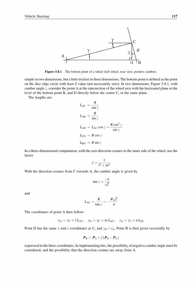
simple in two dimensions, but a little trickier in three dimensions. The bottom point is defined as the point

on the disc edge circle with least Z value (not necessarily zero). In two dimensions, Figure 5.8.1, with

camber angle g, consider the point A at the intersection of the wheel axis with the horizontal plane at the

level of the bottom point B, and D directly below the centre C, in the same plane.

The lengths are:

LAC ¼ R

tan g

LAB ¼ R

sin g

LAD ¼ LAC cos g ¼ R cos2 gsin g

LCD ¼ R cos g

LBD ¼ R sin g

In a three-dimensional computation, with the axis direction cosines to the inner side of the wheel, use the

factor

f ¼ 1

l2 þ m2

With the direction cosines from C towards A, the camber angle is given by

tan g ¼ �nffiffiffif

p

and

LAC ¼ R

tan g¼ �R

ffiffiffif

pn

The coordinates of point A then follow:

xA ¼ xC þ l LAC; yA ¼ yC þ mLAC; zA ¼ zC þ n LAC

Point D has the same x and y coordinates as C, and zD¼ zA. Point B is then given vectorially by

PB ¼ PA þ f ðPD �PAÞ

expressed in the three coordinates. In implementing this, the possibility of negative camber angle must be

considered, and the possibility that the direction cosines are away from A.

Figure 5.8.1 The bottom point of a wheel (left wheel, rear view, positive camber).


5.9 Wheel Steering Axis

For all systems, thewheels and hubs are pivoted about a steering axis, commonly called the ‘kingpin’ axis,

Figure 5.9.1. Nowadays, on cars at least, physical kingpins are no longer used, the steering axis now

usually being defined by upper and lower ball joints on a double-wishbone suspension, or by one ball joint

and the upper pivot point of the strut on a strut system. In front view, the axis is at the kingpin inclination

angle uKI, usually from zero to 20�, giving a reduced kingpin offset b at the ground, measured from the

undistortedwheel centre plane. The inclination angle helps to give space for the brakes.Where the steering

arms are forward (rack in front of the wheel centres) it also gives room to angle the steering arms for

Ackermann geometry. Sometimes a negative offset is used, this giving straighter braking when surface

friction varies between tracks. Zero offset is called centrepoint steering. If the kingpin inclination angle is

also zero, it is called centreline steering. Centrepoint steering gives no steeringmoment from longitudinal

FX forces at the contact patch; centreline steering gives, in addition, zeromoment for longitudinal forces at

thewheel axle height. This latter effect is important because of the variation of rolling resistance on rough

roads, and traction effects.

5.10 Caster Angle

In the side view of Figure 5.9.1(b), the kingpin axis is slanted at the kingpin caster angle uKC, with a value

generally in the range of 0 – 5�. This introduces a mechanical trail, called the caster trail, which acts in

concert with the tyre pneumatic trail. On cars and trucks it is usual for the kingpin axis to pass through the

wheel spin axis C in side view, but this is not essential, and some offsetting of the axis from the centre

enables the caster angle and trail to be independently varied. The caster angle and the associated caster trail

are important in the feel of the steering. In general, the caster angle varies relative to the body, in

suspension bump zS, with

uKC ¼ uKC0 þ «BCas1zS þ «BCas2z2S ð5:10:1Þ

where «BCas1 is the linear bump caster coefficient (SI units rad/m in equations, practical units deg/dm and

deg/inch; to be distinguished from «BC1, the linear bump camber coefficient), and «BCas2 is the quadratic

Figure 5.9.1 Geometry of the steering axis of a wheel.


bump caster coefficient (rad/m2). Relative to the road, the castor angle also varies with the body pitch

angle uB, due to acceleration or braking:

uKC;R ¼ � uB þ uKC0 þ «BCas1zS þ «BCas2z2S ð5:10:2Þ

Caster variation is generally undesirable, but is used deliberately in some cases, for example to offset the

effect of body pitch in braking. The caster angle and axis offset (the kingpin axis towheel centre separation

in side view) give the caster trail, which, in conjunction with the tyre pneumatic trail, is very important in

giving the steering a suitable feel, and also has a significant effect on directional stability because of

steering compliance. The steering feel is adjusted to obtain a desired relationship between lateral force and

total aligning torque, so that the experienced driver can tell from the steering hand wheel torque when the

tyres are approaching their lateral force limit, as expressed in the Gough plot, a graph of FY versus MZ.

Adding caster trail moves the point of maximum steering torque closer to the point of maximum lateral

force, or even beyond it – that is, the steering goes light later.

During cornering, the steering must also support the centrifugal compensation forces on the steering

mechanism, for example the rack and the track rods. This is called centrifugal caster, and reaches a typical

moment about the kingpin of 10Nm.

On a bumpy road, as the wheel rolls the loaded radius constantly varies. The associated change of

effective rolling radius causes changes of wheel angular speed, with associated longitudinal forces on the

tyre, required to provide the angular acceleration. These forces, ofmagnitude about 1 kN, act on the hub at

wheel axis height, and hence disturb the steering. This can be eliminated only by centreline steering.

Another steering disturbance, for front drive, is the side-to-side difference of the component of the

driveshaft torque along the kingpin axis; this is a problemwhere the driveshafts have different inclinations,

because they have different lengths, or where they are momentarily differently inclined because of rough

roads. This is worst for large torques, and hence during acceleration. This also applies to inboard brakes.

5.11 Camber Angle

When the wheel is steered, the kingpin caster angle and kingpin inclination angle affect the camber angle,

and this can therefore influence turn-in, and especially can influence handling in small-radius corners. For

realistic steer angles, a positive kingpin inclination angle causes a positive camber on the outer wheel,

growing roughlywith the steer angle squared, and being typically 0.15� of camber per degree of inclination

at 30� of steer. Positive caster angle causes a negative camber on the outer wheel, approximately

proportional to steer angle, and is typically �0.50� of camber per degree of caster at 30� of steer. The

actual camber angle is

g ¼ g0 þ arccosðsin uKI cos dÞþ uKI þ arccosðsin uKC sin dÞ � 180� ð5:11:1Þ

The effect of steer angle on camber angle may be represented approximately by

gS ¼ «SC1 dþ «SC2d2 ð5:11:2Þ

where «SC1, the linear steer camber coefficient, depends upon the caster angle (�uKC in radians), and «SC2,the quadratic steer camber coefficient, depends on the kingpin angle (1

2uKC in radians), but changes sign

with the sign of d, that is,

«SC1 ¼ �uKC ð5:11:3Þ

«SC2 ¼ 1

2uKIsignðdÞ ð5:11:4Þ


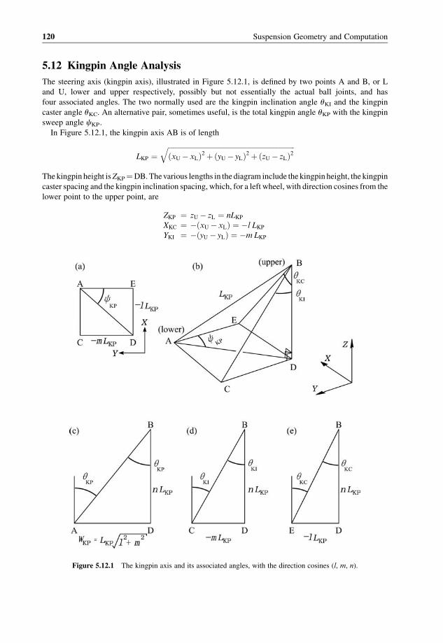
5.12 Kingpin Angle Analysis

The steering axis (kingpin axis), illustrated in Figure 5.12.1, is defined by two points A and B, or L

and U, lower and upper respectively, possibly but not essentially the actual ball joints, and has

four associated angles. The two normally used are the kingpin inclination angle uKI and the kingpin

caster angle uKC. An alternative pair, sometimes useful, is the total kingpin angle uKP with the kingpin

sweep angle cKP.

In Figure 5.12.1, the kingpin axis AB is of length

LKP ¼ffiffiffiffiffiffiffiffiffiffiffiffiffiffiffiffiffiffiffiffiffiffiffiffiffiffiffiffiffiffiffiffiffiffiffiffiffiffiffiffiffiffiffiffiffiffiffiffiffiffiffiffiffiffiffiffiffiffiffiffiffiffiffiffiffiffiffiffiffiffiffiffiffiðxU � xLÞ2 þðyU � yLÞ2 þðzU � zLÞ2

q

The kingpin height isZKP¼DB.Thevarious lengths in the diagram include the kingpin height, the kingpin

caster spacing and the kingpin inclination spacing, which, for a left wheel, with direction cosines from the

lower point to the upper point, are

ZKP ¼ zU � zL ¼ nLKPXKC ¼ �ðxU � xLÞ ¼ �l LKPYKI ¼ �ðyU � yLÞ ¼ �m LKP

Figure 5.12.1 The kingpin axis and its associated angles, with the direction cosines (l, m, n).


The signs are chosen to make the variables normally positive. The diagonal AD is

WKP ¼ffiffiffiffiffiffiffiffiffiffiffiffiffiffiffiffiffiffiffiffiX2KC þ Y2

KI

q¼

ffiffiffiffiffiffiffiffiffiffiffiffiffiffiffil2 þm2

pLKP ¼


pLKP

The angles may be written as

tan uKP ¼ WKP

ZKP¼


p

n

tan cKP ¼ XKC

YKI¼ l

m

tan uKC ¼ XKI

ZKP¼ � l

n

tan uKI ¼ YKI

ZKP¼ �m

n

The relationships between the angles may be deduced from Figure 5.12.1(b):

ZKP tan uKP cos cKP ¼ AE ¼ CD ¼ ZKP tan uKI

so

tan uKI ¼ tan uKP cos cKP

Similarly,

tan uKC ¼ tan uKP sin cKP

Given uKI and uKC initially, the above two equations are easily solved for uKP and cKP. The conversion

equations are summarised in Table 5.12.1. Based on these, various sets of equations may be put together

for the dimensions according to the starting information, for example as in Tables 5.11.2–5.11.5.

Table 5.12.1 Kingpin angle conversion equations

tan uKI ¼ tan uKP coscKP

tan uKC ¼ tan uKP sincKP

tancKP ¼ tan uKCtan uKI

tan uKP ¼ tan uKIcos cKP

¼ tan uKCsin cKP


Table 5.12.3 Static kingpin analysis given lower point L (xL,yL,zL),

HKP, uKI and uKC

xU ¼ xL � ZKP tan uKC

yU ¼ yL � ZKP tan uKI

zU ¼ zL þ ZKP

WKP ¼ ffiffiffiffiffiffiffiffiffiffiffiffiffiffiffiffiffiffiffiffiX2KC þ Y2

KI

p

cKP ¼ atantan uKCtan uKI

� �¼ atan

XKC

YKI

� �

uKP ¼ atanWKP

ZKP

� �

Table 5.12.4 Static kingpin analysis given lower points L (xL, yL, zL),

LKP, uKI and uKC

cKP ¼ atantan uKCtan uKI

� �

uKP ¼ atantan uKCsincKP

� �¼ atan

tan uKIcoscKP

� �

ZKP ¼ LKP cos uKP



zU ¼ zL þ ZKP

Table 5.12.2 Static kingpin analysis given lower point L (xL, yL, zL)

and upper point U (xU, yU, zU)

ZKP ¼ zU � zL

uKI ¼ atan�m

n

� �¼ atan

yL � yU

ZKP

� �

uKC ¼ atan�l

n

� �¼ atan

xL � xU

ZKP

� �

cKP ¼ atanl

m

� �¼ atan

xL � xU

yL � yU

� �

uKP ¼ atan

ffiffiffiffiffiffiffiffiffiffiffiffiffiffiffiffiffiffiffiffiffiffiffiffiffiffiffiffiffiffiffiffiffiffiffiffiffiffiffiffiffiffiffiffiffiffiffiðxL � xUÞ2 þðyL � yUÞ2

qZKP

0@

1A

n ¼ 1ffiffiffiffiffiffiffiffiffiffiffiffiffiffiffiffiffiffiffiffiffiffiffiffiffiffiffiffiffiffiffiffiffiffiffiffiffiffiffiffiffiffiffiffi1þ tan2 uKI þ tan2 uKC

pl ¼ �n tan uKC

m ¼ �n tan uKI


5.13 Kingpin Axis Steered

When a wheel is steered, in a coordinate system rotating with wheel steer angle the caster and inclination

angles, as seen by the wheel, change. With a left wheel and left steer angle d, the wheel sees a kingpinsweep angle

cKPw ¼ cKP þ d

so

XKCw ¼ XKC cos dþ YKI sin d

YKIw ¼ �XKC sin dþ YKI cos d

The variables uKP, LKP, ZKP andWKP are invariant in this transformation. The kingpin angles seen by the

wheel are therefore, for example,

tan uKCw ¼ XKCw

ZKP¼ XKC cos dþ YKI sin d

ZKP

giving

tan uKCw ¼ tan uKC cos dþ tan uKI sin d

and

tan uKIw ¼ �tan uKC sin dþ tan uKI cos d

Approximating the above equations by a quadratic steer angle gives

uKCw ¼ uKC 1� 1

2d2

� �þ uKI d ¼ uKC þ uKI d� 1

2uKC d

2

uKIw ¼ �uKC dþ uKI 1� 1

2d2

� �¼ uKI � uKC d� 1

2uKI d

2

Table 5.12.5 Static kingpin analysis given lower point L (xL,yL,zL),

LKP, uKP and cKP

uKI ¼ atanðtan uKP cos cKPÞuKC ¼ atanðtan uKP sin cKPÞHKP ¼ LKP cos uKP



zU ¼ zL þ ZKP


Representing the kingpin angles seen by the wheel as quadratic expressions

uKCw ¼ uKC þ «SKC1 dþ «SKC2 d2

uKIw ¼ uKI þ «SKI1 dþ «SKI2 d2

the linear and quadratic steer caster coefficients of a left wheel are

«SKC1 ¼ uKI

«SKC2 ¼ �1

2uKC

and the steer inclination coefficients are

«SKI1 ¼ � uKC

«SKI2 ¼ �1

2uKI

These apply to individual wheels, with contrary steer angles on the opposite sides of the vehicle.

5.14 Steer Jacking

Steering of thewheels, in conjunctionwith the kingpin inclination angle uKI, the kingpin caster angle uKC,the caster offset yCO and the caster trail xCT, has the effect of lifting or lowering the steered corner of the

vehicle slightly, affecting the steering feel. The steer jacking effect is positive for a raising of the body

relative to the road, or as a lowering of the wheel relative to the body. Because of the total kingpin

inclination angle uKP, the rotation required about the kingpin axis to give awheel steer angle d is d cos uKP.

Considering first a case of zero inclination angle, we have

zSJ ¼ �xCT cos uKC 1� cosd

cos uKP

� �� sin uKC � yCO sin d sin uKC

Now considering small kingpin angles,

zSJ ¼ �xCT uKC1

2d2 � yCO uC d

Considering now zero caster angle, the effect of the inclination angle is

zSJ ¼ yCO cos uKI 1� cosd

cos uKP

� �� sin uKI þ xCT sin d sin uKI

With the small-angle approximation, this becomes

zSJ ¼ yCO uKI1

2d2 þ xCT uKI d

Considering a quadratic model of the jacking effect,

zSJ ¼ «SJ1 dþ «SJ2 d2


then the single wheel steer jacking coefficients are

«SJ1 ¼ xCT uKI � yCO uKC

«SJ2 ¼ 1

2yCO uKI � 1

2xCT uKC

For a complete axle it is necessary to consider the effects of the two wheels with corresponding steer

angles, negated on one side. The steer jacking effect of the axle is

zSJA ¼ 2«SJ2 d2

with no linear effect. The roll effect is

fSJA ¼ 2«SJ1T

d

with no quadratic effect. The terms tend to compensate each other. The linear term gives asymmetrical

jacking, i.e. no front-end lift but a small roll effect. The second-order term gives a symmetrical effect, so

giving a small front-end lift. Substituting practical values, the effects are small other than at large steering

angles, but can nevertheless be felt by the driver.

References

Durstine, J.W. (1973) The Truck Steering System from Hand Wheel to Road Wheel, SAE 730039, The 19th Ray

Buckendale Lecture, January, SAE SP-374. New York: Society of Automotive Engineers.

Heldt, P.M. (1948) The Automotive Chassis, 2nd edition, Published by P. M. Heldt, 600pp.

Nemeth, J. (1989) Optimization on steering mechanisms for high speed coaches. In Second International Conference

on New Developments in Powertrain and Chassis Engineering, pp. 325–330. Bury St Edmunds: Mechanical

Engineering Publications. ISBN 0852986890.

————— // —————


6

Bump and Roll Steer

6.1 Introduction

A car is usually steered by changes to the angles of the front wheels, controlled by the driver’s handwheel.

However, the geometry of the suspension linkages also results in changes of the steer angle of the wheels

when they move up or down, effects called ‘bump steer’ and ‘roll steer’. All types of steer angle are

represented by dwith an appropriate subscript. In dynamic cornering, the tyre lateral forces are associated

with the tyre slip angles, denoted by a. Careful distinction must be drawn between steer angles d, whichare the angle of the wheel relative to the vehicle centreline, and slip angles a, which are the angle of the

wheel compared with the local direction of motion.

The term ‘bump steer’ means changes of steer angle for a single wheel of an independent suspension

when the wheel is moved up or down relative to the body, in suspension bump and droop. The term ‘roll

steer’ refers to changes of steer of the pair of wheels (i.e. of the axle) when the body rolls. These are

obviously related, but bump steer is the basic form of data for independent suspension, and roll steer is the

basic form for rigid axles. Some forms of bump and roll steer can cause poor straight-line stability, and

very unpredictable and unpleasant vehicle behaviour, the handling being sensitive to small changes of

wheel steer angles. To the driver, a vehicle with significant bump or roll steer, particularly oversteer, may

seem to wander and to be unpredictable.

An axlemay have steer effects because of suspension roll or symmetrical suspension double bump. The

whole vehicle may have steer effects because of heave, pitch or roll of the suspension. All of these effects

can be expressed as steer coefficients relating the wheel angle changes to the stimulus. In summary, the

main geometric steer and camber coefficients are those in Table 6.1.1. The angle units are specified in

radians. These are the correct units for use in equations, although the actual values are often expressed in

degrees. The bump steer coefficient is conveniently expressed as deg/dm (deg/inch US). Angle responses

to angle stimulus have no units, being expressible as rad/rad, which is the same as deg/deg.

6.2 Wheel Bump Steer

The steer angle of a single wheel may be represented as

d ¼ dT0 þ dS þ «BS1 zS þ «BS2 z2S þ � � � ð6:2:1Þ

Here d is the complete road wheel steer angle, dT0 is the initial (static) toe-out angle at zero bump, dS is thewheel steer angle contributed by movement of the driver’s handwheel, «BS1 is the linear bump

steer coefficient, and «BS2 is the quadratic bump steer coefficient. More terms could be added to the

polynomial if desired, although this is only necessary for large suspension motions and high accuracy.


For understanding bump steer, the linear and quadratic terms are sufficient. The linear bump steer

coefficient «BS1 has units rad/m but it is usually expressed in deg/dm (deg/inch US). The quadratic

coefficient «BS2 has fundamental units rad/m2, but is often expressed as deg/dm2. It is normal practice

to express the values in degrees, but radian units should be used in the equations (1 radian¼ 180/p¼57.29578 deg).

In general, the linear bump steer coefficient is defined as the rate of change of wheel steer angle with

vertical wheel position (suspension bump deflection), with the steering hand wheel fixed, of course:

«BS¼ dd

dzSð6:2:2Þ

This will be taken as positive for toe-out with a rising wheel. The first linear bump steer coefficient «BS1 is

the value of this at the static position. A positive quadratic coefficient «BS2 gives toe-out in both bump and

droop, proportional to the square of the bump value.

For any independent front suspension, e.g. the double wishbone of Figure 6.2.1, consider the vehicle

body fixed and the wheel to move in bump with the steering disconnected at B, in a controlled ideal way

with no steer angle change of thewheel. The steering-arm ball joint Bwill thenmove in an arc with centre

at some point A, called the ideal point or ideal centre, where the position of A depends on the particular

suspension geometry. For most real suspensions, the movement of B is not a perfectly circular arc, but an

arc is a good approximation.With the steering nowconnected, if the track rod to rack ball joint, or track rod

to relay rod joint, C, is actually at A then there will be no bump steer. This possibility of achieving an

accurate steering motion is an important advantage of independent suspension over a steered rigid axle.

Predictable and precise handling is particularly important for competition and high-performance vehicles,

and in such cases it is considered to be of paramount importance that the rack is mounted accurately at

the correct height, with a tolerance of only 1 or 2mm, and that the rack and track rods should be of the

appropriate length. In practice, for passenger cars there are often significant production tolerance error

discrepancies of the height, length or alignment of the rack. For ordinary road vehicles complete accuracy

is often not even attempted, deliberate discrepancies being introduced. These are sometimes claimed to

give less wheel response to rough roads or to have handling advantages, although this is a controversial,

and interesting, issue.

The above is a two-dimensional analysis, of course, and in reality the steering and suspension

mechanism is a three-dimensional one. The ‘ideal point’ is really extended in space, usually roughly

Table 6.1.1 The main wheel, axle and vehicle linear steer variables

(1) dBS rad single-wheel bump steer angle

(2) dRS rad axle roll steer angle

(3) dDBS rad axle double-bump steer angle

(4) dRT rad axle roll toe angle

(5) dDBT rad axle double-bump toe angle

(6) «BS1 rad/m single-wheel bump steer coefficient

(7) «RS1 rad/rad axle roll steer coefficient

(8) «RU1 rad/m axle roll understeer coefficient

(9) «DBS1 rad/m axle double-bump steer coefficient

(10) «RT1 rad/m axle roll toe coefficient

(11) «DBT1 rad/m axle double-bump toe coefficient

(12) «VHU1 rad/m vehicle heave understeer coefficient

(13) «VPU1 rad/rad vehicle pitch understeer coefficient

(14) «VRU1 rad/rad vehicle roll understeer coefficient


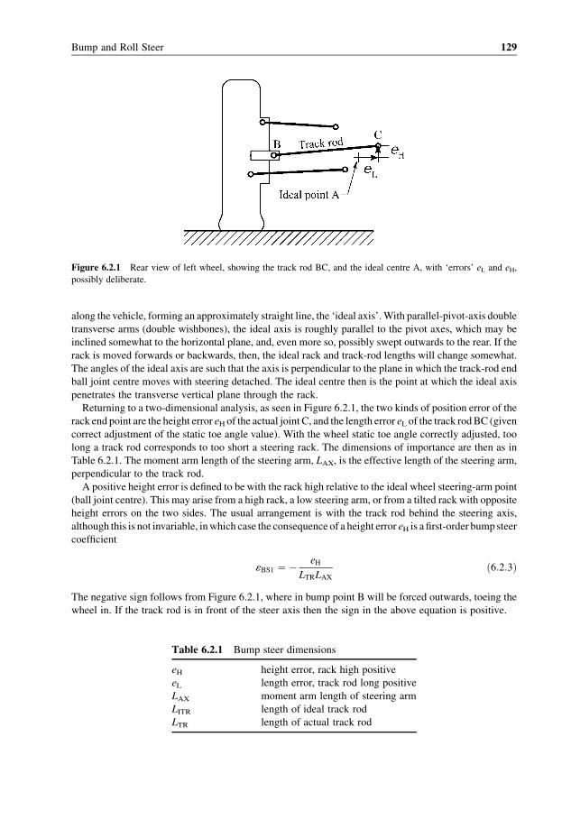
along the vehicle, forming an approximately straight line, the ‘ideal axis’.With parallel-pivot-axis double

transverse arms (double wishbones), the ideal axis is roughly parallel to the pivot axes, which may be

inclined somewhat to the horizontal plane, and, even more so, possibly swept outwards to the rear. If the

rack is moved forwards or backwards, then, the ideal rack and track-rod lengths will change somewhat.

The angles of the ideal axis are such that the axis is perpendicular to the plane in which the track-rod end

ball joint centre moves with steering detached. The ideal centre then is the point at which the ideal axis

penetrates the transverse vertical plane through the rack.

Returning to a two-dimensional analysis, as seen in Figure 6.2.1, the two kinds of position error of the

rack end point are the height error eH of the actual joint C, and the length error eL of the track rodBC (given

correct adjustment of the static toe angle value). With the wheel static toe angle correctly adjusted, too

long a track rod corresponds to too short a steering rack. The dimensions of importance are then as in

Table 6.2.1. The moment arm length of the steering arm, LAX, is the effective length of the steering arm,

perpendicular to the track rod.

A positive height error is defined to be with the rack high relative to the ideal wheel steering-arm point

(ball joint centre). This may arise from a high rack, a low steering arm, or from a tilted rack with opposite

height errors on the two sides. The usual arrangement is with the track rod behind the steering axis,

although this is not invariable, inwhich case the consequence of a height error eH is a first-order bump steer

coefficient

«BS1 ¼ � eH

LTRLAXð6:2:3Þ

The negative sign follows from Figure 6.2.1, where in bump point B will be forced outwards, toeing the

wheel in. If the track rod is in front of the steer axis then the sign in the above equation is positive.

Table 6.2.1 Bump steer dimensions

eH height error, rack high positive

eL length error, track rod long positive

LAX moment arm length of steering arm

LITR length of ideal track rod

LTR length of actual track rod

Figure 6.2.1 Rear view of left wheel, showing the track rod BC, and the ideal centre A, with ‘errors’ eL and eH,

possibly deliberate.

Bump and Roll Steer 129

A positive length error is defined to be with the track rod too long, when adjusted for correct static toe:

eL ¼ LTR � LITR ð6:2:4Þ

This could be due to a rack too short, a steering armmisaligned, or a rack laterally misplaced on the body,

giving antisymmetrical length errors. The result is a quadratic bump steer coefficient

«BS2 ¼ � eL

2LAXL2ITR

ð6:2:5Þ

For an independent suspension, calculation of the ideal pivot centre A for the track rod, Figure 6.2.1, to

give zero bump steer is a purely geometrical problem. However, it really requires a three-dimensional

solution.

In the case of strut suspension, the ideal track-rod length is highly sensitive to the vertical position of

the steering arm, tending to infinity when it is at the strut top, Figure 6.2.2. A common solution is to use

a rack with centre-mounted track rods, and then to choose a rack height for which these are the correct

length, which roughly matches up with the main spring seat. There are various other independent front

suspensions, not often seen nowadays, for which there exist suitable ideal steering layouts free of bump

steer.

If the measured wheel steer angle is plotted against bump, a result such as Figure 6.2.3 is typically

obtained.Actually there is normally also a toe angle at zero bump; this is the static toe, and does not usually

appear in bump steer plots because it is readily adjustable and is measured separately; bump steer is

usually measured only as the change of angle from static.

The measured bump steer can then be characterised in two main ways – the linear and quadratic

components. At zero bump there is a gradient of steer changewith bump, dd/dzS, the tangent to the curve atzero bump,which in this case can bemeasured from the graph as about 0.3� toe-out in 75mmbump, that is,

a bump steer coefficient of þ 4�/m or 0.4�/dm. This linear effect results from the rack height, say about

5mm too low in this case with the rack behind the wheels, or high for the rack in front. Secondly, there is

a curvature of the graph. In this case the curvature is towards toe-in, which would result from a track rod

Figure 6.2.2 For strut suspension, the correct length of the steering arm varies considerably with the vertical position

of the arm.


longer than ideal for a rack behind the wheels, and shorter than ideal for a rack in front of the wheels, as

can be seen by imagining the ideal and actual arcs of the track-rod end. Relative to the tangent at zero

bump, the quadratic bump steer is about 0.5� toe-in in 75mm bump or droop, so the quadratic bump steer

coefficient here is about �90�/m2 or �0.90�/dm2. This would be caused by a rack length error of about

20mm (at each end).

The initial toe-out tendency in bumpmeans that the wheel itself tends to recede from the bump, and so

possibly reduces the steering fight on rough roads. The quadratic-term curvature toes in the inner wheel in

cornering, reducing its slip angle. This can help to prevent undue wear because of excessive slip on the

lightly loaded tyre, an example of the abandonment of ideal Ackermann steering under dynamic

conditions.

Because of the nominal symmetry of the whole steering and suspension system, even if the above

deliberate steer deviations are adopted, symmetrical axle heave (double bump) should not cause net

steering effects, which is an advantage over a steered rigid axle. Nevertheless, the toe-in varies with load

which can affect steering feel and tyre wear, for which reason if bump steer is deliberately introduced it is

best to design it around a light-load position.Where present, bump steer is often a palliative for some other

fault such as bad weight distribution, and is likely to give poor straight-line stability and tyrewear. At best

such effects compromise the basic handling in order to gain some rough road or other small advantages,

and so should be used with caution.

Many cars are designed with zero theoretical bump steer, but positioning of the steering rack is critical

and sufficiently close tolerances are rarely held in production, particularly if this aspectwas not considered

adequately during the design process. Even for a given design, bump steer varies from car to car and even

from side to side of one car, sometimes to the extent that onewheel toes inwith bump and the other toes out.

Unequal bump steer left and right, which is heave steer or double-bump steer, is especially bad for straight-

line stability.

6.3 Axle Steer Angles

Given the individual steer angles of the two independent wheels on an axle, the axle can be considered to

have combined steer angles, these being the symmetrical and antisymmetrical components of the

Figure 6.2.3 Example bump steer graph.


individual wheel steer angles. The symmetrical part is the mean steer angle of the two wheels. The

antisymmetrical part is the toe angle of the axle. Hence, the axle steer angle is

dA ¼ 1

2ðdL þ dRÞ ð6:3:1Þ

and the axle toe angle is

dT ¼ 1

2ðdL � dRÞ ð6:3:2Þ

Given these axle angles, the individual wheel angles may then be deduced as

dL ¼ dA þ dT ð6:3:3Þ

dR ¼ dA � dT ð6:3:4Þ

It is apparent from this that bump steer angles of individual wheels can alternatively be expressed as angle

properties of the complete axle.

If the individual wheel static toe angles of an axle are unequal, normally attributable to improper

adjustment rather than production tolerance error, then the axle will have a static steer angle. On an

unsteered axle, at the rear, this will cause crabbing of the vehicle.

6.4 Roll Steer and Understeer

For a rigid axle, in cornering the suspension roll anglefS can cause a steer angle of thewhole axle as a unit.

This can also occur for an axle with independent wheels, with the additional complication of the effect

of suspension roll on the axle toe angle. Suspension heave (double bump) may also cause steer effects.

The axle steer angle may then be expressed as

dA ¼ dA0 þ «RSfS þ «DBSzS þ � � � ð6:4:1Þ

with other possible terms, where «RS is the linear roll-steer coefficient and «DBS is the linear double-bump

steer coefficient.

The axle roll steer coefficient «RS is the rate of change of axle mean wheel steer angle with respect to

suspension roll angle, and is usually expressed as deg/deg (i.e. degrees of steer per degree of roll), so it is

dimensionless. Formally, the units are rad/rad. For small roll angles, the roll steer angle dRS is given in

terms of the roll steer coefficient and suspension roll angle by

dRS ¼ «RSfS ð6:4:2Þ

For independent suspension, the roll steer coefficient is closely related to the bump steer coefficient, but is

also influenced by vehicle track width. For a rigid axle it relates to the steer angle of the complete axle,

whereas for independent suspension it relates to the mean value for the pair of wheels.

The axle roll understeer angle dRUmust be clearly distinguished from the axle roll steer angle dRS. They

are numerically equal but the sign convention is different. The roll understeer angle is positive when it

requires increased handwheel angle to compensate, that is, when it requires increased driver-applied

steering.

Hence the relationship between roll understeer angle and roll steer angle is that they are the same at the

front, but have change of sign at the rear:

dRUf ¼ þ dRSf

dRUr ¼ � dRSrð6:4:3Þ


This also applies to the relationship between roll understeer and roll steer coefficients:

«RUf ¼ þ «RSf«RUr ¼ � «RSr

ð6:4:4Þ

Corresponding roll oversteer coefficients could be defined, but thesewould simply be negatives of the roll

understeer values.

Axle roll steer is a property of a single axle, whereas axle roll understeer is a property of an axle in the

context of a vehicle, the context defining the attributable sign. Roll understeermay also be a property of the

vehicle as a whole, the vehicle roll understeer resulting from the characteristics of both axles.

The advantage of referring to roll understeer coefficients rather than roll steer coefficients is that in

evaluating the total understeer coefficient or understeer angle the effects are simply added without

constant consideration of a front/rear sign convention. For understeer coefficients,

«RU ¼ «RUf þ «RUr ð6:4:5Þ

whereas for roll steer coefficients the total understeer coefficient is

«RU ¼ «RSf � «RSr ð6:4:6Þ

The sumof the front and rear roll steer coefficients has no simple physicalmeaning in terms of the steering.

If the front and rear axles exhibit equal positive roll steer, the roll understeer is zero, and the steady-state

steering is largely unaffected, but the dynamic responsemay be altered because suspension roll will cause

transient slip angles.

The smooth-road-condition ideal of zero roll steer may be abandoned in some cases, but there are

definite limitations to the amount of roll steer that is acceptable. Roll oversteer of independent front

suspension (i.e. wheel toe-in in bump) gives severe wheel-fight on rough roads. Roll oversteer of the rear

gives increased body attitude angles, a very unpleasant uncertain feeling for the driver, and bad directional

response to rough roads and to side winds.

It does not seem to be effective to balance an oversteering rear with an understeering front, and really

there is little reason to try to do so. In short, there is good reason to avoid roll oversteer at either end.

Some would argue for rear roll understeer for its reduced attitude angle and hence possibly faster

response, especially for large cars which tend to have a larger dynamic index, but this can lead to problems

with rough roads or wind, and may result in engine torque steering because of body roll in strong

acceleration, unless the power is transmitted through an independent or de Dion axle, or an offset lift bar

is used.

6.5 Axle Linear Bump Steer and Roll Steer

Although the geometry of steering variation is, for independent suspension, expressed by the bump steer

coefficients, fromapractical point of view it is the combined action of left and right sides thatmatterswhen

the body moves in roll. Hence, it is necessary to deduce the axle roll steer from the single-wheel bump

steer. Of course this may be done by calculating the individual suspension bump values on each side from

the suspension roll angle fS, the bump steer angles from the suspension bump values, and the roll steer

angles from the bump steer angle values. However, it is also of interest to obtain the roll steer coefficients

directly in terms of the bump steer properties.

Given a linear bump steer angle, with constant bump steer coefficient,

dBS ¼ «BS1zS ð6:5:1Þ


and the relationship between roll angle and individual suspension bump

zS;R ¼ þ 1

2TfS

zS;L ¼ � 1

2TfS

ð6:5:2Þ

then the individual wheel bump steer angles, toe-out positive, are

dBS;R ¼ þ «BS11

2TfS

dBS;L ¼ � «BS11

2TfS

ð6:5:3Þ

To convert these to roll steer angles, there is a sign change on the left, because bump steer is positive for

toe-out on both sides, but roll steer must have the same sign for the same sense of rotation on the two sides

of the car:

dRS;R ¼ þ dBS;RdRS;L ¼ � dBS;L

ð6:5:4Þ

The wheel roll steer angles are therefore

dRS;R ¼ þ «BS11

2TfS

dRS;L ¼ þ «BS11

2TfS

ð6:5:5Þ

The axle mean roll steer angle is therefore

dRS ¼ 1

2ðdRS;R þ dRS;LÞ

¼ 1

22«BS1

1

2TfS

¼�1

2T«BS1

�fS

ð6:5:6Þ

Comparing this with equation (6.5.1), the linear roll steer coefficient is

«RS1 ¼ 1

2T«BS1 ð6:5:7Þ

This is the fundamental relationship between roll steer and bump steer for an independent-suspension

axle.

Because the bump steer angles are equal and opposite in this simple symmetrical case, there is no axle

toe angle resulting from the roll angle.

6.6 Axle Non-Linear Bump Steer and Roll Steer

Consider now the more complex case, with quadratic bump steer included, and also vehicle asymmetries.

The individual suspension bumps are still

zS;R ¼ þ 1

2fST

zS;L ¼ � 1

2fST

ð6:6:1Þ

The wheel bump steer angles are

dBS;R ¼ «BS1;R zS;R þ «BS2;R z2S;R

dBS;L ¼ «BS1;L zS;L þ «BS2;L z2S;L

ð6:6:2Þ


which are therefore

dBS;R ¼ «BS1;R

�þ 1

2fST

�þ «BS2;R

�þ 1

2fST

�2

dBS;L ¼ «BS1;L

�� 1

2fST

�þ «BS2;L

�� 1

2fST

�2 ð6:6:3Þ

These bump steer angles are positive for toe-out on each side, so the equivalentmean roll steer angle for the

complete axle is half of the difference of the bump steer angles of the two wheels:

dRS ¼ 1

2dBS;R � dBS;L� �

Since individual wheel toe-out is positive, this gives positive roll steer corresponding to the axle

effectively turning out of the curve. Hence, this is an understeer effect at the front and oversteer at the

rear. Substituting the above expressions, and noting that a negative valve squared is positive, the axle roll

steer angle becomes

dRS ¼ 1

4fSTð«BS1;R þ «BS1;LÞþ 1

2

�1

2fST

�2

«BS2;R� «BS2;L� � ð6:6:4Þ

Hence the first-order and second-order roll-steer coefficients are

«RS1 ¼ 1

4Tð«BS1;R þ «BS1;LÞ

«RS2 ¼ 1

8T2ð«BS2;R � «BS2;LÞ ð6:6:5Þ

Therefore, any linear bump steer gives linear roll steer. However, symmetrical second-order bump steer

does not give second-order roll steer, which only arises from asymmetrical «BS2.Hence, thiswill tend to be

fairly small, although possibly not insignificant, because it will usually arise from production tolerance

errors rather than from design intent. One feature that can cause it is unequal track-rod lengths in

conjunction with certain types of suspension, a feature which has been used on some passenger cars.

The roll toe angle of the axle is

dRT ¼ 1

2ðdBS;R þ dBS;LÞ

¼ 1

4TfSð«BS1;R � «BS1;LÞþ 1

2

�1

2TfS

�2

ð«BS2;R þ «BS2;LÞð6:6:6Þ

Hence, the first and second roll toe coefficients are

«RT1 ¼ 1

4Tð«BS1;R � «BS1;LÞ

«RT2 ¼ 1

8T2ð«BS2;R þ «BS2;LÞ

ð6:6:7Þ

Therefore, linear roll toe is due to asymmetry of the linear bump steer, due to production tolerance errors

(e.g. a tilted rack). The quadratic roll toe coefficient is due to quadratic bump steer.

Equations (6.6.5) and (6.6.7) also make it possible to deduce the bump steer coefficients from roll steer

and toe steer values. The equations are

«BS1;R ¼ 2

Tð«RS1 þ «RT1Þ

«BS1;L ¼ 2

Tð«RS1 � «RT1Þ

«BS2;R ¼ 4

T2ð«RS2 þ «RT2Þ

«BS2;L ¼ 4

T2ð«RS2 � «RT2Þ

ð6:6:8Þ


6.7 Axle Double-Bump Steer

Consider now an axle bump deflection, which is a suspension double bump, zA, which might occur on

landing after a symmetrical crest, as frequently occurs with some severity on rally cars. The right and left

suspension bumps on the axle are

zS;R ¼ zS;L ¼ zA ð6:7:1Þ

The individual bump steer angles are

dBS;R ¼ «BS1;R zA þ «BS2;R z2A

dBS;L ¼ «BS1;L zA þ «BS2;L z2A

ð6:7:2Þ

These are both positive for toe-out, so the axle (mean double bump) steer angle is given by

dDBS ¼ 1

2ðdBS;R � dBS;LÞ ð6:7:3Þ

which is

dDBS ¼ 1

2zAð«BS1;R � «BS1;LÞþ 1

2z2Að«BS2;R � «BS2;LÞ ð6:7:4Þ

The linear and quadratic double-bump steer coefficients are therefore

«DBS1 ¼ 1

2ð«BS1;R � «BS1;LÞ ð6:7:5Þ

«DBS2 ¼ 1

2ð«BS2;R � «BS2;LÞ ð6:7:6Þ

Hence, both of the double-bump steer coefficients depend upon the side-to-side difference between the

individual bump steer coefficients, and hence upon vehicle asymmetries, normally arising from produc-

tion tolerance errors, for example a tilted rack, although possibly from design asymmetrical track-rod

lengths, etc. The first-order double-bump steer coefficient «DBS1 is particularly critical for straight-line

behaviour on dips and crests, and suitable design and control of production tolerances must be applied to

ensure only a small resulting value.

6.8 Vehicle Roll Steer

Roll of the entire sprungmass gives suspension roll of the front and rear axles, with total steer effects. The

vehicle understeer coefficients follow easily from the axle roll steer coefficients, allowing for the

understeer sign convention for axle position at the front or rear:

«VRU1 ¼ «RUf1 þ «RUr1

«VRU2 ¼ «RUf2 þ «RUr2ð6:8:1Þ

Assuming equal tracks front and rear, by substitution the vehicle roll understeer coefficients are

«VRU1 ¼ 1

4Tð«BS1;fR þ «BS1;fL � «BS1;rR � «BS1;rLÞ

«VRU2 ¼ 1

8T2ð«BS2;fR � «BS2;fL � «BS2;rR þ «BS2;rLÞ ð6:8:2Þ

For the linear coefficient, the units are none, rad/rad or deg/deg as preferred, these having the same

meaning. The quadratic coefficient has units rad–1 or rad/rad2.


6.9 Vehicle Heave Steer

Heave of the entire sprung mass gives double bump of the front and rear axles, with possible steer effects.

For the front axle,

«DBS1;f ¼ 1

2ð«BS1;fR � «BS1;fLÞ

«DBS2;f ¼ 1

2ð«BS2;fR � «BS2;fLÞ ð6:9:1Þ

For the rear axle,

«DBS1;r ¼ 1

2ð«BS1;rR � «BS1;rLÞ

«DBS2;r ¼ 1

2ð«BS2;rR � «BS2;rLÞ ð6:9:2Þ

Summing the effects, allowing for the signs, the vehicle heave understeer coefficients are

«VHU1 ¼ «DBS1;f � «DBS1;r«VHU2 ¼ «DBS2;f � «DBS2;r

ð6:9:3Þ

giving the vehicle heave understeer coefficients finally as

«VHU1 ¼ 1

2ð«BS1;fR � «BS1;fL � «BS1;rR þ «BS1;rLÞ

«VHU2 ¼ 1

2ð«BS2;fR � «BS2;fL � «BS2;rR þ «BS2;rLÞ ð6:9:4Þ

For the linear coefficient, the units are rad/m for use in equations, possibly expressed as deg/m. The

quadratic coefficient has units rad/m2, possibly expressed as deg/m2.

Body heave will also cause axle toe angle effects. The required expressions for these are easily derived

as above.

6.10 Vehicle Pitch Steer

For body pitching about the centre of mass, with suspension pitch angle uS, the axle double bumps are in

the ratio of the partial wheelbases:

zAf ¼ þ a uSzAr ¼ � b uS

ð6:10:1Þ

The vehicle pitch understeer coefficients are therefore

«VPU1 ¼ 1

2að«BS1;fR � «BS1;fLÞ�1

2bð«BS1;rR � «BS1;rLÞ ð6:10:2Þ

«VPU2 ¼ 1

2að«BS2;fR � «BS2;fLÞ� 1

2bð«BS2;rR � «BS2;rLÞ ð6:10:3Þ

For the linear coefficient, the units are none, rad/rad or deg/deg as preferred, these having the same

meaning. The quadratic coefficient has units rad�1 or rad/rad2.

By an adverse accumulation of production tolerance errors, these coefficients may be significant, even

though they are zero in principle for a symmetrical design of vehicle. The main result is a steer effect in

braking, which, combined with reduced stability under braking, can be problematic in extreme cases. The

solution is to hold sufficiently close tolerances on critical dimensions.

Body pitch will also cause toe effects on each axle. The coefficients may be derived as above.


Two other pitch understeer coefficients can be derived. These are for the combined-heave-and-pitch

ride oscillation modes, which have nodes at particular points, depending on the body inertia and

suspension stiffnesses. The coefficient for a mode follows by methods similar to the above, once the

nodal position for that mode has been determined (e.g. Dixon, 2007).

6.11 Static Toe-In and Toe-Out

A small static toe-in at the rear often has a surprisingly large effect on handling, increasing understeer;

front-wheel-drivevehicles, being lightly loaded at the rear, and therefore having a large rear tyre cornering

stiffness coefficient, are especially sensitive to this. Front toe-out might be expected to have the same

effect. However, practical experience shows the reverse: front toe-out gives a vague steering feel, whereas

front toe-in gives a favourable feel and leads to increased understeer that can bemeasured on the skid pad.

This seems to be caused by the combination of load transfer, aligning torque, lateral force on caster trail,

and steering compliance. Too much front toe-in affects corner turn-in, giving an unprogressive and

imprecise steering feel.

Static toe settings are governed within quite narrow bands by tyre wear. For the least wear, toe settings

should be arranged to give minimal steer angles when running, regardless of small static camber angles.

This means a small static toe-in for undriven wheels, and a small toe-out for driven ones, so that when the

vehicle is running normally the tractive forces and compliances act to bring the toe angles close to zero.

Within the allowable band for low wear (a total range of about 1�), there is only limited scope to use toe

angles to tune the handling characteristics.

6.12 Rigid Axles with Link Location

Rigid rear axles can be considered in two groups: thosewith link location and thosewith longitudinal leaf

springs. In the case of link location, there are lateral location points A and B according to the particular

linkages, defining an axis of rotation of the axle relative to the body. Figure 6.12.1 shows a general

four-link axle. The method is based on studying the support links to find two points A and B where forces

are exerted by the axle on the body. The line through the two points is the axis of rotation of the axle

relative to the body. The roll centre lies on this line, at the point where it penetrates the transverse vertical

Figure 6.12.1 A rigid axle with link location to the body has two location points which define the relative axis of

rotation. This position and inclination angle of this axis gives the roll centre and the roll steer coefficient.


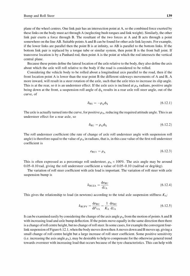
plane of the wheel centres. One link pair has an intersection point at A, so the combined force exerted by

these links on the body must act through A (neglecting bush torques and link weight). Similarly, the other

link pair exerts a force through B. The resultant of the two forces at A and B acts through a point

somewhere on the line AB. Suitable points A and B can be found for other axle link layouts. For example,

if the lower links are parallel then the point B is at infinity, so AB is parallel to the bottom links. If the

bottom link pair is replaced by a torque tube or similar system, then point B is the front ball joint. If

transverse location is by a Panhard rod, then point A is the point at which the rod intersects the vertical

central plane.

Because these points define the lateral location of the axle relative to the body, they also define the axis

about which the axle will roll relative to the body if the road is considered to be rolled.

Considering the vehicle body to be rolled about a longitudinal axis parallel to the road, then if the

front location point A is lower than the rear point B the different sideways movements of A and B, A

more inward, will result in a steer rotation of the axle, such that the axle tries to increase its slip angle.

This is at the rear, so it is an understeer effect. If the axle axis is inclined at rA radians, positive angle

being down at the front, a suspension roll angle of fS results in a rear axle roll steer angle, out of the

curve, of

dRS ¼ �rAfS ð6:12:1Þ

The axle is actually turned into the curve, for positive rA, reducing the required attitude angle. This is anundersteer effect for a rear axle, so

dRU ¼ rAfS ð6:12:2Þ

The roll understeer coefficient (the rate of change of axle roll understeer angle with suspension roll

angle) is therefore equal to the value of rA in radians, that is, in this case value of the first roll understeer

coefficient is

«RU1 ¼ rA ð6:12:3Þ

This is often expressed as a percentage roll understeer, rA� 100%. The axis angle may be around

0.05–0.10 rad, giving the roll understeer coefficient a value of 0.05–0.10 (rad/rad or deg/deg).

The variation of roll steer coefficient with axle load is important. The variation of roll steer with axle

suspension bump is

kRUZA ¼ d«RUdzA

ð6:12:4Þ

This gives the relationship to load (in newtons) according to the total axle suspension stiffness KA:

kRUFV ¼ d«RUdFVA

¼ 1

KA

d«RUdzA

ð6:12:5Þ

It can be examined easily by considering the change of the axis angle rA from themotion of pointsA andB

with increasing load and axle bump deflection. If the points move equally in the same direction then there

is a change of roll centre height, but no change of roll steer. In some cases, for example the convergent four-

link suspension of Figure 6.12.1,when the bodymoves down thenAmoves downandBmoves up, giving a

small change of roll centre height but a large increase of roll steer coefficient. Some positive sensitivity

(i.e. increasing the axis angle rA), may be desirable to help to compensate for the otherwise general trend

towards oversteer with increasing load that occurs because of the tyre characteristics. This can help with


primary understeer but does not help with final understeer or oversteer, for which the roll centre height is

the dominant factor.

It might appear in the above discussion that the axle axis angle should be measured relative to the

vehicle roll axis rather than to the horizontal. However, thevehicle does not in a real sense roll about its roll

axis. Rolling the body about the inclined roll axis implies a roll about a horizontal axis plus a yaw

movement which will affect front and rear suspensions equally, and so will have no net result on the

steering angle required.

6.13 Rigid Axles with Leaf Springs

In the case of longitudinal leaf springs, the roll steer coefficient depends on the inclination of the equivalent

link AB that describes the motion arc of the wheel centre, Figure 6.13.1. This equivalent link is directed

towards the unshackled end, is about three-quarters of the length of that end of the spring, and is roughly

parallel to it.When the body rolls, point A rises on the inner side and falls on the outer, thus tending to steer

the axle.Horizontal equivalent links give no steer, because both sidesmove forward equally.HavingpointA

higher than B gives roll oversteer for a rear axle (i.e. reduced slip angle tendency), B higher gives roll

understeer. For a front axle the effects are opposite. The roll steer coefficient is equal to the AB line

inclination angle expressed in radians, independent of the spring length or separation.On the other hand, the

spring length affects the influence of load variation on roll steer coefficient. Too high a coefficient, apart

from being bad for handling, also leads to harshness on rough roads because of thewheel path in bump, and

other problems. EarlyHotchkiss axles, before 1930,were given a negative roll-steer coefficient because this

resulted in less sensitivity to road roughness. In the early 1930s a positive coefficient was first used (i.e. roll

oversteer was replaced by roll understeer) and a dramatic increase in directional stability was found.

6.14 Rigid Axles with Steering

Before the introduction of independent front suspension, all cars had a rigid front axlewith steering. They

suffered from a variety of rather severe steering problems.

When the rigid axle with longitudinal leaf springs is used at the front, as on some trucks and off-road

vehicles even today, it is subject to all the effects described earlier, plus additional effects because of the

steering linkage. The critical steering link is always the one that connects the sprung and unsprung parts of

the steering. Figure 6.14.1 shows a typical arrangement with front steering and a rear spring shackle. Here

CD is the drag link, D is the connection to thewheel hub, and C is the connection to the Pitman arm on the

steering box, fixed to the sprung mass. When the axle moves, D has an ideal no-steer arc centred on the

ideal centre E. If E and C do not coincide, there will be steering errors. As early as the 1920s, it was

attempted tomatch the E andCpositions for rollmotions, butwith disappointing results. The reason is that

the arc of D is different for each of roll, single-wheel bump, and heave, and different again with braking

Figure 6.13.1 Rigid axle with location by leaf springs, without steering.


because of axle wind-up. Also there are differences because of production variability of springs, and

variation between spring options. One improvement that is sometimes adopted is to use an unsprung

steering box, the sprung to unsprung connecting linkage being through a splined steering column.

In the early days, before the introduction of front independent suspension, the steering errors of rigid

front axleswere a real problem. The usualway to dealwith the problemwas to use stiff springs tominimise

the axle movement. When independent suspension was introduced, as discussed in Chapter 1, it became

possible to use much softer front suspension springing having greater deflections without unacceptable

bump steer and roll steer problems, allowing implementation of the now better-understood relationship

between front and rear stiffnesses that give good ride qualities – with the front springs softer than the rear

to give the desired pitch and heave oscillation mode qualities and mode nodal positions.

References

Dixon, J.C. (2007) The Shock Absorber Handbook. Chichester: John Wiley & Sons, Ltd. ISBN 9780470510209.

————— // —————

Figure 6.14.1 Rigid axle with leaf-spring location and steering.


7

Camber and Scrub

7.1 Introduction

Camber is angling of the wheel from the vertical, in front or rear view. Scrub is lateral movement of the

bottom point of the wheel. These are controlled by similar factors in the suspension geometry, and so are

dealt with together.

Wheel camber relative to the road surface affects the tyre lateral forces. The camber angle variation

with suspension bump depends on the position of the swing centre, introduced here. The swing centre also

affects the scrub rate and the roll centre position. For an independent suspension, the wheel camber

variation is described by the bump camber. For a complete independent axle, the coefficients can be

expressed as symmetrical and antisymmetrical properties of the axle. Themain angles and coefficients are

as in Table 7.1.1. The units shown are the fundamental SI ones, as normally required for use in equations.

Actual values are, however, often quoted in other units, particularly degrees instead of radians, and inches

instead of metres in the USA. There are also several important bump scrub coefficients, leading to heave,

double bump and roll scrub coefficients.

7.2 Wheel Inclination and Camber

The symbol for tyre slip angle isa, but a different symbol, d, is used for steer angles, including bump steer.

There is no accepted symbol for a deliberate alteration of camber angle, since steering is not controlled in

that way. Hence, g is used here and elsewhere for all types of wheel camber. The distinction should be

borne in mind, however, between the different effects represented by g, especially those corresponding tothe distinction between d anda. There can be camber angles relative to the vehicle body, corresponding to

d, and camber angles relative to the road surface, corresponding to a. The body roll angle f then

corresponds to the attitude angle b.A distinctionmust also bemade between the inclination angle and the camber angle. For a givenwheel,

these have the same magnitude but with a different sign convention. Inclination is positive for right-hand

rotation about the forward longitudinal axis, which is clockwise in rear view. Camber is positive with the

top of the wheel outward from the vehicle centreline, Figure 7.2.1. Here, the wheel inclination angle

will be represented by G (Greek capital gamma), whereas the wheel camber angle will be denoted by g(Greek lower case gamma).

The basic relationship between the inclination and camber angles for the two sides of the vehicle is

therefore simply that on the right-hand side they are the same, but on the left-hand side there is a change


of sign:

GR ¼ þ gRGL ¼ � gL

ð7:2:1Þ

There is a small static camber setting on a wheel, denoted g0. On a passenger car this is chosen to

minimise wear. On a racing car it is almost invariably negative. The wheel camber relative to the body

changes as the suspension moves in bump, Figure 7.2.2. The bump camber angle of a single wheel, gBC,is the increase of camber angle, compared with the static value, due to suspension bump deflection zS.

For a linear model, the total camber angle at a given suspension bump is

g ¼ g0 þ gBC ð7:2:2Þ

Linearly, the bump camber angle is

gBC ¼ «BC1zS ð7:2:3Þ

Table 7.1.1 Camber and inclination angles and coefficients

(1) g0 the static wheel camber angle (rad)

(2) gBC the wheel bump camber angle (rad)

(3) GA the axle inclination angle (rad)

(4) gA the axle camber angle (rad)

(5) «BC the wheel bump camber coefficient (rad/m)

(6) «ARI the axle roll inclination coefficient (—, rad/rad, deg/deg),

(7) «ARC the axle roll camber coefficient (rad/rad)

(8) GP the path section inclination angle (rad).

Figure 7.2.1 Wheel inclination angle and camber angle sign convention: (a) positive inclination, rear view only;

(b) positive camber, front or rear view.


where the linear bump camber coefficient «BC1 depends on the suspension geometry, and would be

positive for positive-going camber on a rising wheel. The basic units of the bump camber coefficient are

rad/m, although commonly expressed as deg/dm (deg/inch in the USA). The bump camber coefficient is

usually negative for practical designs. More elaborately, including a second-order term,

g ¼ g0 þ «BC1zS þ «BC2z2S þ � � � ð7:2:4Þ

where «BC2 is the quadratic bump camber coefficient.

7.3 Axle Inclination and Camber

The axle line is the line joining the centres of the twowheels at the opposite ends of the axle. Here, the term

‘axle’ is applied broadly to include the two wheels of an independent suspension. The wheel inclination

angle and camber angle aremeasured from the perpendicular to the axle line.Axle roll angle (the roll angle

of the axle line) and road surface transverse-section angles also affect the camber of the wheel relative to

the road, but are accounted for separately, Figure 7.3.1. When there is suspension roll, the individual

wheels are in suspension bump and have camber changes relative to the body. For an independent

suspension, thesewheel cambers can be accounted for separately, but it is also possible towork in terms of

the symmetrical and antisymmetrical axle values, the axle mean inclination and the axle mean camber,

respectively. In Figure 7.3.1(d) note that, with clockwise rotation positive, a negative path inclination

gives a positive wheel inclination relative to the road.

The axle mean inclination angle (nothing to do with the axle roll angle) is the mean of the inclination

angles of the two wheels of the axle:

GA ¼ 1

2ðGR þGLÞ ð7:3:1Þ

For an ideally symmetrical vehicle, this is zero. By substitution, it is equal to the semi-difference of the

wheel camber angles, arising from constructional imperfections or compliance camber:

GA ¼ 1

2ðgR � gLÞ ¼ gd ð7:3:2Þ

The antisymmetrical component, called the axle camber angle, is the semi-difference of the inclination

angles,

gA ¼ 1

2ðGR �GLÞ ð7:3:3Þ

Figure 7.2.2 Suspension bump causes wheel camber angle change (rear view).

Camber and Scrub 145

This is also equal to the mean of the camber angles:

gA ¼ 1

2ðgR þ gLÞ ¼ gm ð7:3:4Þ

Then the individual right and left wheel inclination angles are

GR ¼ GA þ gAGL ¼ GA � gA

ð7:3:5Þ

Figure 7.3.1 Wheel/road camber caused by: (a) antisymmetrical suspension bump; (b) suspension roll camber;

(c) rigid axle roll on tyre vertical stiffness; (d) road section shape.

Figure 7.3.2 Axle mean inclination GA and axle camber gA together give the individual wheel inclinations.


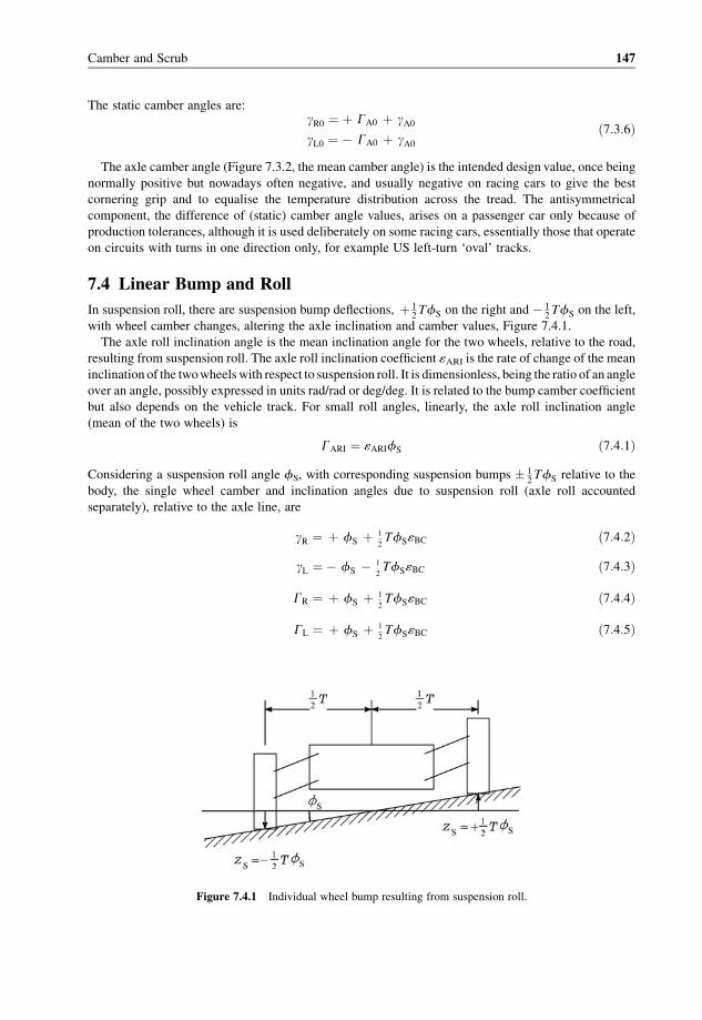
The static camber angles are:gR0 ¼ þ GA0 þ gA0gL0 ¼ � GA0 þ gA0

ð7:3:6Þ

The axle camber angle (Figure 7.3.2, the mean camber angle) is the intended design value, once being

normally positive but nowadays often negative, and usually negative on racing cars to give the best

cornering grip and to equalise the temperature distribution across the tread. The antisymmetrical

component, the difference of (static) camber angle values, arises on a passenger car only because of

production tolerances, although it is used deliberately on some racing cars, essentially those that operate

on circuits with turns in one direction only, for example US left-turn ‘oval’ tracks.

7.4 Linear Bump and Roll

In suspension roll, there are suspension bump deflections, þ 12TfS on the right and � 1

2TfS on the left,

with wheel camber changes, altering the axle inclination and camber values, Figure 7.4.1.

The axle roll inclination angle is the mean inclination angle for the two wheels, relative to the road,

resulting from suspension roll. The axle roll inclination coefficient «ARI is the rate of change of the mean

inclination of the twowheelswith respect to suspension roll. It is dimensionless, being the ratio of an angle

over an angle, possibly expressed in units rad/rad or deg/deg. It is related to the bump camber coefficient

but also depends on the vehicle track. For small roll angles, linearly, the axle roll inclination angle

(mean of the two wheels) is

GARI ¼ «ARIfS ð7:4:1Þ

Considering a suspension roll angle fS, with corresponding suspension bumps � 12TfS relative to the

body, the single wheel camber and inclination angles due to suspension roll (axle roll accounted

separately), relative to the axle line, are

gR ¼ þ fS þ 1

2TfS«BC ð7:4:2Þ

gL ¼ � fS � 1

2TfS«BC ð7:4:3Þ

GR ¼ þ fS þ 1

2TfS«BC ð7:4:4Þ

GL ¼ þ fS þ 1

2TfS«BC ð7:4:5Þ

Figure 7.4.1 Individual wheel bump resulting from suspension roll.


The axle mean inclination angle is

GA ¼ 1

2ðGR þGLÞ

¼ fS þ 1

2TfS«BC

¼ ð1þ 1

2T«BCÞfS

ð7:4:6Þ

Hence the fundamental relationship between the linear axle roll inclination coefficient and the linear

wheel bump camber coefficient is

«ARI ¼ 1þ 1

2T«BC ð7:4:7Þ

Bump camber coefficients are usually made negative in order to reduce «ARI, to offset the effect of bodyroll on wheel inclination, Figure 7.4.2. To be explicit, equation (7.4.7) may be inverted into the design

equation for the necessary bump camber for a desired roll inclination coefficient:

«BC ¼ 2

Tð«ARI � 1Þ ð7:4:8Þ

For example, the axle roll inclination coefficientwould typically be 0.5 (rad/rad), requiring a bumpcamber

coefficient value of �1/T (rad/m), about �0.7 rad/m.

A rigid axle is not subject to suspension roll inclination or camber, but it does roll because suspension

roll leads to axle roll as a result of load transfer on the tyre vertical stiffness. Very loosely, then, a solid axle

might be said to have an axle roll camber coefficient, typically of about 0.12 (deg/deg) for a passenger car,

although this is not a real geometric effect. This axle roll on the tyres is also applicable to independent

suspensions. However, this is not normally accounted for as an axle inclination angle change. It is a roll of

the wheel-centres axle line:

fA ¼ kfAfSfS ð7:4:9ÞThe complete inclination angles of the wheels relative to the path surface are therefore, Figure 7.4.3,

including path inclination angles, given by the path angle contact point to contact point, minus the local

path inclination angle, plus the axle roll angle plus the wheel inclination relative to the axle:

GW=P ¼ ðfP þfA þGWÞ� ðfP þGPÞ ð7:4:10Þ

Figure 7.4.2 Suspension roll causes wheel inclination.


where the path inclination angle GP is measured relative to the path bank angle fP. To be specific, noting

that the path bank angle is eliminated, the left and right inclination angles relative to the path (road) are:

GW;R ¼ fA þGR �GP;R ¼ fA þðgR0 þfS þ 1

2T«BCfSÞ�GP;R ð7:4:11Þ

GW;L ¼ fA þGL �GP;L ¼ fA þð� gL0 þfS þ 1

2T«BCfSÞ�GP;L ð7:4:12Þ

7.5 Non-Linear Bump and Roll

Considering non-linear bump and roll suspension characteristics, and also asymmetrical characteristics,

the basic wheel camber angles are

gR ¼ gR0 þfS þ «BC1;RzS þ «BC2;Rz2S

gL ¼ gL0 �fS þ «BC1;LzS þ «BC2;Lz2S

ð7:5:1Þ

Substituting zS ¼ � 1

2fTS, the inclination angles are

GR ¼ þ gR0 þ fS þ 1

2T«BC1;RfS þ 1

4T2«BC2;Rf

2S

GL ¼ � gL0 þ fS þ 1

2T«BC1;LfS � 1

4T2«BC2;Rf

2S

ð7:5:2Þ

The axle mean inclination angle is

GA ¼ 1

2ðGR þGLÞ

¼ 1

2ðgR0 � gL0ÞþfS þ 1

4Tð«BC1;R þ «BC1;LÞfS þ 1

8T2ð«BC2;R � «BC2;LÞf2

S

ð7:5:3Þ

This may be expressed in terms of the axle roll inclination coefficients as

GA ¼ GA0 þ «ARI1fS þ «ARI2f2S ð7:5:4Þ

with the three terms

GA0 ¼ 1

2ðgR0 � gL0Þ ð7:5:5Þ

Figure 7.4.3 Wheel inclination angles relative to the local path surface.


«ARI1 ¼ 1þ 1

4Tð«BC1;R þ «BC1;LÞ ð7:5:6Þ

«ARI2 ¼ 1

8T2ð«BC2;R � «BC2;LÞ ð7:5:7Þ

The first of these,GA0, is the asymmetrical production tolerance error on static camber. The second, «ARI1,

is the linear axle roll inclination coefficient, and depends on the sum of thewheel first-order bump camber

coefficients. The final term, «ARI2, is the quadratic axle roll inclination coefficient, which therefore

depends on design asymmetry and production tolerance asymmetry giving different second-order bump

camber coefficients.

The axle camber is

gA ¼ 1

2ðGR �GLÞ

¼ 1

2ðgR0 þ gL0Þþ 1

4Tð«BC1;R � «BC1;LÞfS þ 1

8T2ð«BC2;R þ «BC2;LÞf2

S

ð7:5:8Þ

This may be expressed as

gA ¼ gA0 þ «ARC1fS þ «ARC2f2S ð7:5:9Þ

with the three terms

gA0 ¼ 1

2ðgR0 þ gL0Þ ð7:5:10Þ

«ARC1 ¼ 1

4Tð«BC1;R � «BC1;LÞ ð7:5:11Þ

«ARC2 ¼ 1

8T2ð«BC2;R þ «BC2;LÞ ð7:5:12Þ

The first of these, gA0, is the mean static camber of the two wheels, arising from production tolerances.

The second, «ARC1, is the linear axle roll camber coefficient, and depends on the production tolerance

difference of the wheel first-order bump camber coefficients. The final term, «ARC2, is the quadratic axleroll camber coefficient which depends on the sum of the wheel second-order bump camber coefficients.

An ideal symmetrical vehicle can therefore be expected to exhibit zero second-order axle roll

inclination and zero first-order axle roll camber.

7.6 The Swing Arm

At any given bump position, for a further infinitesimal increment of the suspension in bump, thewheel has

an instantaneous centre of rotation relative to the body, point E in Figure 7.6.1. In general kinematics, an

instantaneous centre of rotation is known as a ‘centro’. In vehicle dynamics, in this particular case it is

called the swing arm centre or just swing centre. For some suspensions (e.g. a swing axle) this centro is a

fixed point on the body, while for others (e.g. wishbones, struts) the point depends on the suspension

geometry in a more complex way, and moves relative to the body, so the coordinates of E depend on the

suspension bump position zS.

Point F is the notional wheel contact point with the ground. This is in the vertical transverse section of

the suspension, that is, in the section shown in Figure 7.6.1, in the longitudinal plane of the notionally

undistorted wheel, and at the level of the bottom point of the wheel. In cornering, the tyre has substantial

lateral distortion, but point F excludes this, being in the wheel centre plane. Point H is the foot of the

perpendicular from the swing centreE to the level of the bottomof thewheel. Length FE is called the swing

arm length, whereas the horizontal length FH is called the swing arm radius (SAE definitions).


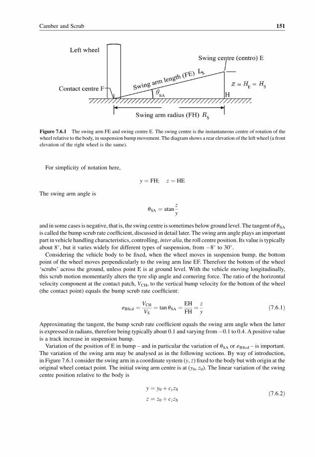
For simplicity of notation here,

y ¼ FH; z ¼ HE

The swing arm angle is

uSA ¼ atanz

y

and in some cases is negative, that is, the swing centre is sometimes belowground level. The tangent of uSAis called the bump scrub rate coefficient, discussed in detail later. The swing arm angle plays an important

part invehicle handling characteristics, controlling, inter alia, the roll centre position. Its value is typically

about 8�, but it varies widely for different types of suspension, from �8� to 30�.Considering the vehicle body to be fixed, when the wheel moves in suspension bump, the bottom

point of the wheel moves perpendicularly to the swing arm line EF. Therefore the bottom of the wheel

‘scrubs’ across the ground, unless point E is at ground level. With the vehicle moving longitudinally,

this scrub motion momentarily alters the tyre slip angle and cornering force. The ratio of the horizontal

velocity component at the contact patch, VCH, to the vertical bump velocity for the bottom of the wheel

(the contact point) equals the bump scrub rate coefficient:

«BScd ¼ VCH

VS

¼ tan uSA ¼ EH

FH¼ z

yð7:6:1Þ

Approximating the tangent, the bump scrub rate coefficient equals the swing arm angle when the latter

is expressed in radians, therefore being typically about 0.1 and varying from�0.1 to 0.4. A positive value

is a track increase in suspension bump.

Variation of the position of E in bump – and in particular the variation of uSA or «BScd – is important.

The variation of the swing arm may be analysed as in the following sections. By way of introduction,

in Figure 7.6.1 consider the swing arm in a coordinate system (y, z) fixed to the body but with origin at the

original wheel contact point. The initial swing arm centre is at (y0, z0). The linear variation of the swing

centre position relative to the body is

y ¼ y0 þ cyzS

z ¼ z0 þ czzSð7:6:2Þ

Figure 7.6.1 The swing arm FE and swing centre E. The swing centre is the instantaneous centre of rotation of the

wheel relative to the body, in suspension bumpmovement. The diagram shows a rear elevation of the left wheel (a front

elevation of the right wheel is the same).


7.7 Bump Camber Coefficients

Referring again to Figure 7.6.1, the incremental change of single-wheel camber angle for an increment

of suspension bump is

dg ¼ � 1

ydzS

so the rate of change of camber with suspension bump is

dgdzS

¼ �1

y0 þ cyzSð7:7:1Þ

In the special case of cy¼ 0, with the swing centre moving only vertically,

g ¼ g0 �zS

y0ð7:7:2Þ

Otherwise, by integration of equation (7.7.1) (e.g. Spiegel, 1968, 14.59), from zS¼ 0,

g ¼ g0 �1

cyloge 1þ cyzS

y0

� �ð7:7:3Þ

The vertical variation of the swing centre position, coefficient cz, plays no part in this. Expanding the

logarithm as a series,

logeð1þ xÞ ¼ x� 1

2x2 þ 1

3x3 � 1

4x4 þ � � �

gives

g ¼ g0 �zS

y0þ 1

2cy

zS

y0

� �2

� � � � ð7:7:4Þ

which for cy¼ 0 reduces to the earlier simplified case solution. Matching the polynomial expression for

camber, from equation (7.2.4), which was

g ¼ g0 þ «BC1zS þ «BC2z2S

gives the bump camber coefficients in terms of the swing-arm centre initial position and its movement

coefficient cy:

«BC1 ¼ � 1

y0ð7:7:5Þ

«BC2 ¼ cy

2y20ð7:7:6Þ

7.8 Roll Camber Coefficients

Substitutingequations (7.7.5)and(7.7.6) into(7.5.6)onwards, the linearandquadratic roll inclinationandroll

camber coefficients may be expressed in terms of the swing centre movement coefficients. The results are:

«ARI1 ¼ 1� 1

4T

1

y0;Rþ 1

y0;L

� �ð7:8:1Þ


«ARI2 ¼ 1

8T2 cy;R

2y20;R� cy;L

2y20;L

!ð7:8:2Þ

«ARC1 ¼ �1

4T

1

y0;R� 1

y0;L

� �ð7:8:3Þ

«ARC2 ¼ 1

8T2 cy;R

2y20;Rþ cy;L

2y20;L

!ð7:8:4Þ

7.9 Bump Scrub

The basic bump scrub polynomial, for the actual wheel lateral scrub value s, using the basic bump scrub

coefficients «BSc, is

s ¼ yC�yC0 ¼ «BSc1zS þ «BSc2z2S þ «BSc3z

3S þ � � � ð7:9:1Þ

with the initial scrub being zero at static ride height. The local bump scrub rate is the derivative of the

above:

«BScd ¼ ds

dzS¼ «BSc1 þ 2 «BSc2zS þ 3 «BSc3z

2S þ � � � ð7:9:2Þ

However, this is usually expressed in terms of the bump scrub rate coefficients «BScd0, «BScd1, «BScd2, etc.:

«BScd ¼ «BScd0 þ «BScd1zS þ «BScd2z2S þ � � � ð7:9:3Þ

The bump scrub rate coefficients are more convenient than the actual scrub polynomial coefficients when

the roll centre is being analysed, so it is easier to use the rate coefficients throughout, with, when required,

«BSc1 ¼ «BScd0

«BSc2 ¼ 1

2«BScd1 ð7:9:4Þ

«BSc3 ¼ 1

3«BScd2

. . .

so the actual scrub then becomes

s ¼ «BScd0zS þ 1

2«BScd1z

2S þ 1

3«BScd2z

3S þ � � � ð7:9:4Þ

The initial bump scrub rate coefficient, Figure 7.9.1(a), at static ride height, is

«BScd0 ¼ z0

y0ð7:9:5Þ

Allowing for movement of the suspension and of the wheel itself, in terms of the body-fixed swing-centre

coordinates (y,z) Figure 7.9.1(b), the instantaneous bump scrub rate is

«BScd ¼ z� zS

y

Using

z ¼ z0 þ czzS

y ¼ y0 þ cyzS


then

«BScd ¼ z0 þðcz � 1ÞzSy0 þ cyzS

ð7:9:6Þ

Consider initially the simplified case with swing centre movement being vertical only (cy¼ 0), giving

«BScd ¼ z0 þðcz � 1ÞzSy0

ð7:9:7Þ

The variation of the bump scrub variation coefficient is then

d«BScddzS

¼ cz�1

y0ð7:9:8Þ

Therefore, when the suspension geometry is such that cz¼ 1 it follows that the derivative of the bump

scrub variation is zero, and the bump scrub variation coefficient will remain constant in bump. Some

designers hold this to be a desirable condition, as it fixes the roll centre height.

More generally, including cy, by the standard derivative of the quotient expression in equation (7.9.7),

d«BScddzS

¼ ðy0 þ cyzSÞðcz � 1Þ � ðz0 þðcz � 1ÞzSÞcyðy0 þ cyzSÞ2

¼ ðcz � 1Þy0 � cyz0

ðy0 þ cyzSÞ2ð7:9:9Þ

Setting cy¼ 0, this agrees with the simpler earlier expression.

Consider the general bump scrub rate variation, from equation (7.9.3),

«BScd ¼ «BScd0 þ «BScd1zS þ «BScd2z2S þ � � �

The implications of a linear variation, at least, will be explained further later. The coefficient values in the

polynomial may be found in terms of the swing centre variation, viz.:

«BScd0 ¼ z0

y0

«BScd1 � d«BScddzS

¼ ðcz � 1Þy0 � cyz0

ðy0 þ cyzSÞ2

Figure 7.9.1 Variation of the bump scrub coefficient with bump: (a) initial position; (b) in bump the point E rises by

z¼ czzS whilst the wheel rises by zS.


At zS¼ 0, then,

«BScd1 ¼ ðcz � 1Þy0 � cyz0

y20ð7:9:10Þ

Alternatively, use a curve fit to computer-solved point values.

The bump scrub variation, using equation (7.9.7), may be expressed as

ds

dzS¼ «BScd ¼ z� zS

y¼ z0 þðcz � 1ÞzS

y0 þ cyzS

¼ ðz0 þðcz � 1ÞzSÞðy0 þ cyzSÞ�1

¼ ðz0 þðcz � 1ÞzSÞ�

1

y0

��1þ cy

y0zS

��1

The series expansion of (1þ x)�1 (e.g. Spiegel, 1968, equation 20.8) is

1

1þ x¼ 1� x þ x2 � x3 þ � � �

so

ds

dzS¼�

1

y0

�ðz0 þðcz � 1ÞzSÞ

�1� cy

y0zS þ

�cy

y0

�2

z2S � � � ��

¼�

1

y0

��z0 þ

�ðcz � 1Þ� cyz0

y0

�zS þ � � �

�

giving

ds

dzS¼ z0

y0þ ðcz � 1Þy0 � cyz0

y20

� �zS þ � � �

Integrating, with zero scrub at zero suspension bump,

s ¼ z0

y0

� �zS þ ðcz � 1Þy0 � cyz0

2y20

� �z2S þ � � �

Comparing this with the actual scrub polynomial (7.9.5) in terms of the scrub rate coefficients, which was

s ¼ «BScd0zS þ 1

2«BScd1z

2S þ 1

3«BScd2z

3S þ � � �

then

«BScd0 ¼ z0

y0

«BScd1 ¼ ðcz � 1Þy0 � cyz0

y20

ð7:9:11Þ

agreeing with equation (7.9.11). Further terms are easily obtained.


7.10 Double-Bump Scrub

In symmetrical double-wheel bump, equivalent to a negative suspension heave, for independent

suspension there is track change due to scrub and camber change. For a symmetrical axle the axle

inclination is unchanged, with the introduction of symmetrical negative camber (on an independent axle).

Positive scrub causes a track increase. There may be asymmetries due to production tolerance errors,

but these are generally small compared with the bump steer effects.

7.11 Roll Scrub

Geometrically, roll of the suspension will change the axle track due to bump scrub. The total track change,

to second order, is

DT ¼ TðcosfS�1Þþ�«BSc0;R

�1

2TfS

�þ 1

2«BSc1;R

�1

2TfS

�2�þ�«BSc0;L

��1

2TfS

�þ 1

2«BSc1;L

��1

2TfS

�2�

¼ T��1

2f2S

�þð«BSc0;R � «BSc0;LÞ

�1

2TfS

�þ 1

2

�«BSc1;R þ «BSc1;L

�1

2TfS

�2¼n

1

2T�«BSc0;R � «BSc0;L

�ofS þ

n�1

2T þ

�1

8T2��

«BSc1;R þ «BSc1;L

�of2S

ð7:11:1Þ

For an ideal symmetrical vehicle the first-order roll scrub is therefore zero, the linear wheel camber angles

compensating each other. There is a second-order term, partially due to the cosine effect on wheel spacing

and partially due to the second-order wheel bump scrub. For an ideal symmetrical vehicle,

DT ¼ �1

2T 1� 1

2T«BSc1

n of2S ð7:11:2Þ

For an asymmetrical vehicle,

«RSc1 ¼ 1

2Tð«BSc0;R � «BSc0;LÞ

«RSc2 ¼ �1

2T þ 1

8T2ð«BSc1;R þ «BSc1;LÞ ð7:11:3Þ

7.12 Rigid Axles

The nature of non-independent live axles effectively precludes substantial misalignment of the wheels,

which remain effectively parallel, with zero geometric axle inclination and camber. The one exception to

this is in some racing classes, nowmainly historical, where the axleswere ‘tweaked’ in a hydraulic press to

give a small amount of static negative camber, and possibly some toe angle.

DeDion axles, where thewheels are rigidly connected to each other but the drive differential is attached

to the sprung mass, may have static negative camber and toe angle, but this is constant, not varying as for

independent suspension.

References

Spiegel, M.R. (1968) Mathematical Handbook of Formulas and Tables. New York: McGraw-Hill.

————— // —————


8

Roll Centres

8.1 Introduction

This chapter deals with the roll centre for independent suspension. Rigid axles are covered in Chapter 13.

Actually, the idea of the roll centre was introduced early in the days of vehicle dynamics, when all cars

had a rigid axle at both front and rear. The roll axis is a straight line through the front and rear roll centres.

With the introduction of independent suspension, these conceptswere carried over despite some confusing

complications, such as track change in bump and roll, and continued to be the basis of dynamic cornering

analysis. Over the years since then, the roll centre concept has been subject to some criticism, but clarified

and improved.

Really, for a thorough understanding, it is necessary to appreciate that the idea of a single roll centre for

a suspension is only an approximation. There are actually several different types of roll centre, and these

definitions are not exactly equivalent. Also, different authors have used different definitions for the roll

centre of any particular type, none of which are necessarily wrong – each may be good if used correctly.

Third, the roll centre, in general, however defined, is not necessarily a single point, it moves around when

there is suspension bump or roll. Finally, the roll centre as defined may not even be a point, but may be a

range of positions.

Originally, the roll centre idea was, in practice, essential for manual computation of vehicle cornering

dynamics. With the introduction of computers, it became entirely practical to make the necessary

calculations without reference to a roll centre at all. However, the idea of a roll centre remains a valuable

toolforhumanunderstandingofthesuspensioncharacteristics, in thedesignprocess,andasabasisforsimple

calculations or as a summary of the suspension characteristics as found by computer-produced results.

In the simple model of suspension, there is a single roll centre, fulfilling several functions. In reality,

there are several distinct functions, with distinct roll centres:

(1) the geometric roll centre (GRC);

(2) the kinematic roll centre (KRC);

(3) the force roll centre (FRC);

(4) the moment roll centre (MRC).

Historically, for the most part, as a useful practical approximation, these have all been treated as one fixed

point of the suspension. For a thorough understanding, it is necessary to appreciate the differences.

The GRC is a property of the suspension geometry, a point found by specified geometric methods.

The KRC is the point about which the body rolls relative to the axle. This then controls the consequent

lateral position of the sprung centre of mass, affecting the total load transfer.


The FRC is a point at which the suspension links exert a lateral force on the sprung mass. This is

represented, in essence, by the FRCheight, which affects the roll angle of the body and themeans of lateral

load transfer through the suspension links.

The MRC is the point about which moments are taken in dynamic analysis of the body. For a true

dynamic analysis, the front and rearMRCs should generally be on the longitudinal principal axis of inertia.

The traditional method of working, for steady-state analysis at least, was that the various roll centres on

an axle were all deemed to be at one point. This point was found by solving the GRC position, which was

then used,with some justification, as the FRCand theKRC, and even theMRC, allowing practical solution

of vehicle dynamics problems.

The assumptions behind the various roll centres are somewhat different. There is an analogy here with

the lever, for which the mechanical advantage equals the velocity ratio only for zero friction. The usual

analysis of the FRC neglects joint friction and stiffness.

In this book, the emphasis is on geometric properties of roads and suspensions, so this is not the place

for a thorough analysis of all roll centre issues. Here, only the GRCwill be investigated in detail. The FRC

and KRC will be reviewed, however, to show their relationship to the GRC. For a more detailed

explanation of these, see, for example, Dixon (1996).

8.2 The Swing Arm

Figure 8.2.1 shows the basic swing arm constructions, in the two dimensions of the transverse vertical plane

of the suspension, for themain types of independent suspension. Point F is thewheel-to-road contact point,

considering thewheel and tyre to be undistorted (i.e. in the centre plane of thewheel). Tyre distortion effects

such as overturning moment are dealt with separately. Point E is the swing centre. For an unrolled

symmetrical vehicle, the swing arms for the two sides intersect at the centre, this intersection being theGRC

for the symmetrical unrolled position (i.e. at small lateral accelerations only). In practice, for a simple

analysis, the roll centre is assumed not to move relative to the body. The GRC found by this means

(geometric analysis as in Figure 8.2.1) is then considered to indicate the KRC and FRC positions. In fact,

these are not really the same, and the GRC moves relative to the body, as discussed later in this chapter.

Briefly, the swing arm constructions are as follows. Figure 8.2.1(a) shows the double-wishbone sus-

pension (double A-arm), where the motion of one end of a link relative to the other end must be per-

pendicular to the link line between centres. This neglects rubber bush compliance. Therefore, themotion of

thewheel relative to the body, in bump, at each link connection,must be perpendicular to the link. Therefore

the link lines are radii from the instantaneous centre of rotation,which is found by intersecting the link lines,

giving the swing centre E. For the symmetrical case, the roll centre is always in the centre plane, so it is at the

intersection of the swing arm with the centreline.

For the strut of Figure 8.2.1(b), the top slider is like an infinitely long wishbone perpendicular to the

slider. For the pure straight slider suspension of Figure 8.2.1(c), the bottom point of the wheel obviously

moves parallel to the slider, so the swing centre is at infinity, with the swing arm perpendicular to the slider

direction.

Figure 8.2.1(d) shows a driven swing axle, where thewheel is located by the driveshaft, with a universal

joint at the side of the final drive unit. This joint acts as the swing centre, giving point E. This is unusual in

that the swing centre is on the same side of the vehicle as the wheel. The initial roll centre follows at R,

which is notable for being very high. Figure 8.2.1(e) shows a lateral swinging arm with longitudinal axis.

This is known as low-pivot swing arm, producing a desired lower roll centre.

Figures 8.2.1(f,g,h) showvarious forms of trailing arm. The simplest case is (f) inwhich the pivot axis is

perpendicular to the vehicle centre plane, and therefore parallel to the ground. The motion of the wheel

relative to the body is a linear parallel action, so the swing centre is at infinity, and the initial roll centre

is at ground level. In case (g), the trailing arm axis is inclined in rear view only. The body-fixed wheel

motion is parallel but inclined, so the swing centre is again at infinity, but nowwith an inclined swing arm.

Finally, for the general-case trailing arm of case (h), the arm axis is not perpendicular to the vehicle


Figure 8.2.1 Swing arm constructions for unrolled symmetrical vehicles of various independent suspensions:

(a) double wishbones; (b) strut; (c) slider; (d) swing axle; (e) swing arm; (f) trailing arm; (g) trailing arm with

inclination; (h) trailing arm with inclination and plan-view axis rotation. F is the (undistorted) contact patch centre

point, E is the swing centre, R is the roll centre (Dixon, 1991).

centreline in plan view. The projected axis therefore intersects the vertical transverse plane of the

suspension at a non-infinite swing arm length, at swing centre E.

Over the last century of vehicle suspension analysis, many versions of the above swing arm and roll

centre diagrams have been published. The fact that they have often differed shows that even basic

Roll Centres 159

suspension analysis is by no means trivial. Figure 8.2.1, which first appeared in Dixon (1991), seems to

have stood the test of time. Admittedly, however, this is not exactly correct. It is a two-dimensional

approximation to a problem which should really be solved in three dimensions. That said, the

approximation is quite a good one.

8.3 The Kinematic Roll Centre

The very name ‘roll centre’ suggests a kinematic concept, andmany authors do introduce the roll centre as

a point about which the vehicle body rolls. Unfortunately, this is not really true, and the more one thinks

about it themore confusing it can become, considering lateral velocity of thevehicle in cornering and track

changes of the axle.

The essential point of the KRC is that it could be defined as follows (temporary definition):

The kinematic roll centre is the point, in the transverse vertical plane of the suspension, about which

the body rolls in cornering, relative to the axle.

Here, the term ‘axle’ is used in a broad sense tomean the pair of wheels, even if independently sprung. For

independent suspension, the axle track (tread) can change, so the axle lateral position is deemed to be the

mean lateral position of the bottom of the two wheels, considering their undistorted wheel planes.

For a rigid axle, track change is not an issue.

The simplest case is a rigid axle using a sliding block lateral location. This is not used on passenger cars,

but has been used in racing, particularly as a modification to lower the roll centre of some designs of rigid

rear-axle linkage. There is a vertical channel on the axle, carrying a sliding block. The centre of the block

carries a pin aboutwhich the bodymay rotate in roll, Figure 8.3.1. Alternatively, the channelmay be on the

body, and the block and pin on the axle. There is a differencewhen the body is rolled, because heave of the

body perpendicular to the road may or may not cause axle sway (lateral motion) according to the system

chosen. The channel on the axle is usually preferred. Independent suspensions have a similar problem,

according to the design.

Here, it is clear that the body can pivot (i.e. roll) about the pin. Equally apparent is that the block and pin

can, and generally will, move up or down in cornering. Typically the suspension springs are rising rate,

so in roll the body tends to rise, an effect called spring jacking. If the body rolls and rises, then the complete

motion relative to the axle is a rotation about a point offset to one side, Figure 8.3.2.

For simplicity, neglect the tyre deflections. Coordinate YP is positive to the right. For a suspension roll

angle fS and a body heave zB, the mean of the two wheel suspension droops, the lateral offset of the

effective pivot point is

YP ¼ zB

tan fS

ð8:3:1Þ

Figure 8.3.1 Sliding block lateral location of the body on a rigid axle. The body pivots on a pin in the block, which

slides in the channel attached to the axle.


This is evidently, in a sense, the roll centre of the body relative to the axle, but the lateral offset is governed

by the properties of the springs, not the suspension links.

In practical application, the lateral offset of the pivot point, as seen above, is not considered as part of the

roll centre action. The application of the KRC is in calculating the lateral offset of the centre of mass

relative to the axle, a dimension which governs the additional load transfer. In practice therefore, a

different definition is applied:

At a suspension roll anglefS,with resulting centre ofmass offsetYCM relative to the axlemeanwheel

position, the KRC is in the vehicle centre plane and the axle vertical transverse plane, at the KRC

height HKRC, where

HCM �HKRC ¼ YCM

tanfS

ð8:3:2Þ

in which HCM is the initial height of the body centre of mass.

As actually used, the KRC position is derived from the GRC position, and the centre of mass offset,

positive to the right, is calculated as

YCM ¼ ðHCM �HKRCÞtanfS ð8:3:3Þas in Figure 8.3.3.

This offset of the centre ofmass offsets the bodyweight forcemBg, causing a supplementary rollmoment

MYCM ¼ mBgYCM ð8:3:4Þ

Figure 8.3.2 Relative rotation point of the body relative to the axle when the body rises as it rolls, front view.

Figure 8.3.3 Lateral displacement of the centre of mass due to roll angle about the KRC at height HKRC.

Roll Centres 161

This is usually much smaller than the load transfer moment directly due to lateral forces but may still

be significant, depending on the suspension roll stiffness and consequent roll angle. A high roll centre

at both ends of the vehicle therefore reduces the roll angle and the total load transfer. However, in

contrast, a property of the force roll centre is that a higher roll centre at one axle increases the load

transfer on that axle and reduces it on the other axle, this being an important factor in limit handling

adjustment. These conflicting effects of the KRC and FRC have caused some confusion, and even

controversy.

The common practice is to take the KRC height to be the same as the GRC height, in the vehicle

coordinates, neglecting any GRC lateral offset for the reasons stated above, with the GRC found by

geometric analysis of the suspension linkage. In the case of a simple rigid axle, as in Figure 8.3.1,

combined with the defining principle of Figure 8.3.3, this is reasonable. This is also fairly clear for other

rigid axle location systems, such as the Panhard rod.

In the case of independent suspension, the justification is less clear-cut, and reference must be made

to other texts (e.g. Dixon, 1996) for a fuller discussion. The problem is the complication introduced by

the track change of an independent suspension in roll. The swing arm defines the motion of each wheel

relative to the body, sowith some approximations it is reasonable to take the intersection point of the swing

arms (i.e. the GRC), as the putative KRC, and then neglect any a lateral offset (i.e. again to take the height

of the KRC as being the same as the height of the GRC, in vehicle coordinates).

8.4 The Force Roll Centre

The height of the FRC controls two important factors:

(1) the suspension link lateral load transfer;

(2) the suspension link jacking force.

Figure 8.4.1(a) shows the tyre normal (Z) and lateral (Y) force components on the two wheels of an

independent-type axle. This is after removal of forces that support and accelerate the unsprung mass, so

it is for the forces supporting and accelerating the sprung mass (body) only. The coordinate system used

here is the standard ISO one, with X forward, Y to the left, and Z upwards. The tyre forces are shown in

vehicle coordinates. The tyre forces are usually expressed in road normal and lateral coordinates. The road

surface is in general rotated by the roll angle, and also by the two road camber angles. The vehicle-axis

components shown are easily derived. Figure 8.4.1(b) shows these forces resolved instead along (F2) and

perpendicular (F1) to the swing arms. The F1 parts, perpendicular to the swing arms, must be supported

by the springs (and dampers in unsteady state). The F2 parts act through the links, and, as may be seen in

the figure, will exert no moment about the intersection point of the swing arm lines. This conclusion may

be drawn, for a double-wishbone suspension for example, on the basis that the swing arm is the

intersection of the lines of the links, and the links carry link-aligned forces only, that is, that the joints

at the ends of the links are free of stiffness moments (e.g. rubber bushes) and free of friction moments

(e.g. rotating metal sleeve bushes). This is a standard principle of the analysis of pin-jointed structures.

These are evidently engineering approximations, which could be improved upon in a more detailed

analysis, including bush friction or stiffness moments. The lateral position of the GRC is B, positive to

the left.

Figure 8.4.1(c) shows the link force alone resolved back into normal and lateral components. The link

jacking force, which is the total vertical force in the links, relieves the springs of load, causing jacking of

the body. This link jacking force is

FLJ ¼ F2;R sin uSA;R � F2;L sin uSA;L ð8:4:1Þ


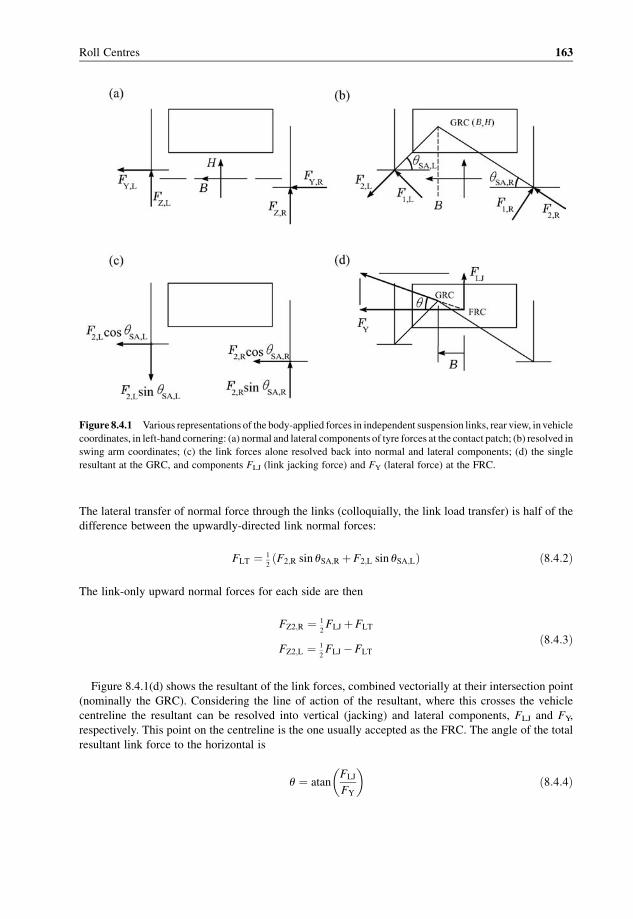
The lateral transfer of normal force through the links (colloquially, the link load transfer) is half of the

difference between the upwardly-directed link normal forces:

FLT ¼ 1

2ðF2;R sin uSA;R þF2;L sin uSA;LÞ ð8:4:2Þ

The link-only upward normal forces for each side are then

FZ2;R ¼ 1

2FLJ þFLT

FZ2;L ¼ 1

2FLJ �FLT

ð8:4:3Þ

Figure 8.4.1(d) shows the resultant of the link forces, combined vectorially at their intersection point

(nominally the GRC). Considering the line of action of the resultant, where this crosses the vehicle

centreline the resultant can be resolved into vertical (jacking) and lateral components, FLJ and FY,

respectively. This point on the centreline is the one usually accepted as the FRC. The angle of the total

resultant link force to the horizontal is

u ¼ atanFLJ

FY

� �ð8:4:4Þ

Figure 8.4.1 Various representations of the body-applied forces in independent suspension links, rear view, invehicle

coordinates, in left-hand cornering: (a) normal and lateral components of tyre forces at the contact patch; (b) resolved in

swing arm coordinates; (c) the link forces alone resolved back into normal and lateral components; (d) the single

resultant at the GRC, and components FLJ (link jacking force) and FY (lateral force) at the FRC.

Roll Centres 163

so the height of the FRC is

HFRC ¼ HGRC �BFLJ

FY

� �ð8:4:5Þ

In Figure 8.4.1(d), B is positive, so HFRC is less than HGRC.

The roll moment exerted by the lateral link force about a central axis at ground level is

MFYL ¼ FYHFRC ¼ FLTT ð8:4:6Þso the FRC height is

HFRC ¼ MFYL

FY

¼ FLTT

FY

ð8:4:7Þ

The load transfer factor fLT is defined as

fLT ¼ FLT

FY

¼ HFRC

Tð8:4:8Þ

so

HFRC ¼ fLTT

FLT ¼ fLTFY

ð8:4:9Þ

This is sufficient not only to illustrate the close relationship between the FRC and the GRC, but also to

illustrate that they are not identical because of the necessary assumptions and approximations, and the

lateral offset.

The actual distribution of forces left and right depends on the tyre characteristics, so only the

approximate position of the FRC can be calculated on the basis of the links alone, the height difference

from the GRC depending on the inclination of the link force resultant.

The anti-roll coefficient JAR is defined as

JAR ¼ HFRC

HB

ð8:4:10Þ

and is usually expressed as a percentage, JARpc¼ JAR� 100%.

8.5 The Geometric Roll Centre

The GRC has already been mentioned several times. Its basic definition is simply as follows:

The geometric roll centre is a point in the transverse vertical plane of the suspension, being the

intersection point of the two swing arm lines, one from each side.

Therefore, once the geometric constructions for the swing arms are understood, theGRC follows easily, as

in Figure 8.4.1(b).

Difficulties arise with the above simple definition when the swing arms are parallel. This divides into

two cases. The first case is as for simple unrolled trailing arms – the swing arms may be overlaid in the

ground surface, with the intersection point anywhere along the swing arm lines. The second case arises,

for example with simple trailing arms in the rolled position, when the swing arms are parallel and do not

intersect at any point. This may occur with or without infinitely long swing arms, which is not important

in this context.


In the first case, the problem is solved simply by extending the definition to say thatwhen the swing arms

overlap, in the road surface, the intersection point is to be taken as on the vehicle centreline, in the road

surface.

When the swing arms are parallel and non-overlapping, as occurs for simple rolled trailing arms or for

rolled equal parallel wishbones, regardless of swing arm length, the GRC is at infinity, either to the left or

right. An infinitesimal change of one swing arm angle, say due to a slight asymmetry, can shift it from one

side to the other. If they are even slightly away from parallel, then the GRC exists in the usual way.

Projecting an infinite intersection point back into the vehicle centreline does not solve the problem of the

KRC, because thevertical position of the infiniteGRC, invehicle coordinates,may be anywherewithin the

range of the swing arm heights. In this specific case, then, the GRC is really of no help.

The case of parallel swing arms can occur for most suspension types, at one double bump position for

any given roll angle. It is exemplified by the simple parallel trailing arm suspension in the rolled position,

as in Figure 8.5.1. TheKRC is on the centreline at ground level. The FRC is found as the point in the centre

plane about which the link forces exert zero moment. The link forces are simply parallel, and the outer

wheel will generate more cornering force, in general, so the FRC tends to be up towards the swing arm of

the outer wheel, according to the relative magnitude of the forces.

8.6 Symmetrical Double Bump

The simplest case of GRC movement is for a symmetrical vehicle in symmetrical double bump,

Figure 8.6.1. With a symmetrical axle bump zA each suspension bump is zA. The local bump scrub

rate coefficients are equal, by symmetry, for the linear case

eBScd ¼ eBScd0 þ eBScd1zA

The GRC height, in the body-fixed coordinates, is

H ¼ zA þ 1

2TeBScd ð8:6:1Þ

Substituting for the bump scrub coefficient, linear in this case, then

H ¼ zA þ 1

2TðeBScd0 þ eBScd1zAÞ ð8:6:2Þ

Figure 8.5.1 Parallel swing arms on a simple rolled trailing-arm suspension.

Roll Centres 165

with

H0 ¼ 1

2TeBScd0 ð8:6:3Þ

Typically, the linear bump scrub variation coefficient eBScd1 is negative, but the GRC rises relative to the

body, remaining on the centreline. The vertical motion of the GRC, relative to the body, in relation to the

suspension double bump, by differentiating equation (8.6.2), is

eH1;DB ¼ dH

dzA¼ 1þ 1

2TeBScd1 ð8:6:4Þ

This value occurs frequently in GRC equations. Relative to the road, the GRC height is

Z ¼ H� zA ð8:6:5Þso

Z ¼ 1

2TðeBScd0 þ eBScd1zAÞ ð8:6:6Þ

With a negative linear bump scrub rate coefficient eBScd1, the GRC falls relative to the road. The vertical

motion of the GRC, relative to the road, in response to suspension double bump, is

eZ1;DB ¼ dZ

dzA¼ 1

2TeBScd1 ð8:6:7Þ

Evidently, the relationship between the variation relative to the body and that relative to the road is

eH1;DB ¼ 1þ eZ1;DB ð8:6:8Þ

For example, with T¼ 1.40m, eBScd1¼�0.6m�1, zA¼ 50mm, relative to the body the GRC goes up by

H�H0 ¼ zAð1 þ 1

2TeBScd1Þ

¼ 50ð1þ 0:5� 1:4� ð�0:6ÞÞ ¼ 50ð1� 0:42Þ ¼ 29 mm

On the other hand, relative to the ground the GRC goes up by

Z � Z0 ¼ zA

�1

2TeBScd1

�

¼ 50ð0:5� 1:4� ð�0:6ÞÞ ¼ 50ð�0:42Þ ¼ �21 mm

that is, it goes down by 21mm relative to the road.

Figure 8.6.1 A symmetrical vehicle shown in vehicle-fixed coordinates: (a) static; (b) with symmetrical double

bump.


If non-linear bump scrub variation is included, then

H ¼ zA þ 1

2TðeBScd0 þ eBScd1zA þ eBScd2z2AÞ ð8:6:9Þ

Z ¼ 1

2TðeBScd0 þ eBScd1zA þ eBScd2z2AÞ ð8:6:10Þ

and the relationship between the two variation rates is preserved. The height H can also be expressed as

H ¼ 1

2TeBScd0 þ 1þ 1

2TeBScd1

� �zA þ 1

2TeBScd2z2A

¼ H0 þ eZ1;DBzA þ 1

2TeBScd2

� �z2A

ð8:6:11Þ

8.7 Linear Single Bump

Figure 8.7.1 shows the geometry formovement of theGRC relative to the bodywhen there is single-wheel

bump, here taken to be on the left-hand side. Here, for simplicity, the small track variation is neglected.

Vehicle bump scrub asymmetry is included. The GRC moves upwards or downwards, and to one side,

generally towards the rising wheel. In body coordinates, the GRC is at (B,H), with B positive to the left. It

is easy to write two simultaneous equations for H:

H ¼ 1

2T þB

� �eBScd;R

H ¼ 1

2T �B

� �eBScd;L þ zL

ð8:7:1Þ

These must be solved for B and H, in the usual way. Eliminating H by subtraction,

0 ¼ 1

2TðeBScd;R � eBScd;LÞþ BðeBScd;R þ eBScd;LÞ� zL ð8:7:2Þ

Using the notation subscript L þ R to denote the addition of terms, L�R for subtraction (and later L�R

for multiplication), i.e.

eBScd;L þR ¼ þ eBScd;RþL ¼ eBScd;L þ eBScd;ReBScd;L � R ¼ � eBScd;R � L ¼ eBScd;L � eBScd;ReBScd;L � R ¼ þ eBScd;R� L ¼ eBScd;L � eBScd;R

ð8:7:3Þ

Figure 8.7.1 An asymmetrical vehicle with single (left) bump, rear view, in vehicle coordinates.

Roll Centres 167

equation (8.7.2) is more compactly expressed as

0 ¼ 1

2TeBScd;R�L þBeBScd;RþL� zL

so the lateral GRC position becomes (with L�R, not R�L, and a corresponding sign change)

B ¼ zL þ 1

2TeBScd;L�R

eBScd;RþL

ð8:7:4Þ

Eliminating B from equations (8.7.1), by appropriate multiplication and addition of equations,

HeBScd;LþR ¼ 1

2T2eBScd;R�L þ zLeBScd;R

so

H ¼ TeBScd;R�L þ zLeBScd;ReBScd;RþL

ð8:7:5Þ

From equation (8.7.4) with zL¼ 0, the initial GRC lateral offset due to asymmetry at zero bump is

B0 ¼ 1

2T

eBScd0;L�R

eBScd0;RþL

� �ð8:7:6Þ

In the symmetrical-vehicle case, this reduces to zero. From equation (8.7.5), the initial height of the GRC,

in body-fixed coordinates, is

H0 ¼ TeBScd0;R � L

eBScd0;R þ L

� �ð8:7:7Þ

In the symmetrical case, this reduces to

H0 ¼ 1

2TeBScd0 ðsymmetrical vehicleÞ ð8:7:8Þ

To go into further detail, the general form of bump scrub rate eBScd must be replaced by actual values, or

by more detailed equations. Considering the case of linear variation of bump scrub rate, with bump on the

left wheel only, we may write

eBScd;L ¼ eBScd0;L þ eBScd1;LzLeBScd;R ¼ eBScd0;R

ð8:7:9Þ

Using equation 8.7.4, the GRC lateral position is then

B ¼ zL þ 1

2TðeBScd0;L�R þ eBScd1;LzLÞ

ðeBScd0;RþL þ eBScd1;LzLÞ ð8:7:10Þ

The variation of this with left bump zL may be found by the standard derivative of a quotient:

d

dx

uðxÞvðxÞ

� �¼

vdu

dx� u

dv

dxv2


This can be applied to equation 8.7.10, then setting zL¼ 0 to obtain the value at static ride height, which is

the GRC lateral position variation in single bump:

eB1;SB ¼ dB

dzL

� �ZL¼0

ð8:7:11Þ

The result is

eB1;SB ¼ 1þ TeBScd0;LeBScd1;LeBScd0;RþL

ð8:7:12Þ

In the symmetrical-vehicle case this reduces to

eB1;SB ¼ 1

2eBScd0þ 1

2TeBScd1 ðsymmetrical vehicleÞ ð8:7:13Þ

Applying the same form of analysis to the GRC vertical position variation in left bump, substituting

equation (8.7.9) into (8.7.5) gives

H ¼ TeBScd0;RðeBScd0;L þ eBScd1;LzLÞþ zLeBScd0;ReBScd0;RþL þ eBScd1;LzL

ð8:7:14Þ

Taking the derivative of a quotient and then setting zL¼ 0 gives the GRC vertical position variation in

single bump:

eH1;SB ¼ dH

dzL

� �ZL¼ 0

ð8:7:15Þ

with the value

eH1;SB ¼ eBScd0;RðeBScd0;RþL þ TeBScd0;ReBScd1;LÞe2BScd0;RþL

ð8:7:16Þ

In the symmetrical-vehicle case, this reduces to

eH1;SB ¼ 1

2ð1þ 1

2TeBScd1Þ ðsymmetrical vehicleÞ ð8:7:17Þ

which is just half of the symmetrical double-bump effect.

8.8 Asymmetrical Double Bump

Figure 8.8.1 shows thegeometry formovement of theGRC relative to the bodywhen there is asymmetrical

double-wheel bump. The small track variation is neglected. Vehicle bump scrub asymmetry is included.

In body coordinates, the GRC is at (B,H). Again, it is easy to write two simultaneous equations for H,

the GRC height in vehicle-fixed coordinates:

H ¼ zR þ 1

2T þB

� �eBScd;R

H ¼ zL þ 1

2T �B

� �eBScd;L

ð8:8:1Þ

Roll Centres 169

Eliminating H by subtraction,

0 ¼ zR � zL þ 1

2TeBScd;R�L þBeBScd;RþL

so

B ¼ ðzL � zRÞþ 1

2TeBScd;L�R

eBScd;RþL

ð8:8:2Þ

To obtain H, eliminate B by multiplication and addition of equations (8.8.1),

HeBScd;LþR ¼ zReBScd;L þ zLeBScd;R þ 1

2T2eBScd;R�L

so

H ¼ ðzReBScd;L þ zLeBScd;RÞþ TeBScd;R�L

eBScd;RþL

ð8:8:3Þ

Touse equation (8.8.2) or (8.8.3) in specific cases, it is necessary to substitute specific values, or equations,

for the bump scrub rate coefficients (e.g. constant, linear variation, or other polynomials). The variation

coefficients for B and H with the left and right bumps may be derived, but are not particularly useful.

However, the above results are very general, and can be used to obtain results for specific cases of

combined heave and roll, expressed as equivalent bumps.

In the case of a symmetrical vehicle, equation (8.8.2) for the GRC lateral position becomes

B ¼ðzL�zRÞ 1þ 1

2TeBScd1

� �2eBScd0 þðzL þ zRÞeBScd1 ðsymmetrical vehicleÞ ð8:8:4Þ

Equation (8.8.3) for the GRC height does not simplify usefully, so it is better to evaluate the bump scrub

rates at the two bump positions and use equation (8.8.3) as it is.

Figure 8.8.1 A vehicle with asymmetrical double bump, rear view, in vehicle coordinates.


8.9 Roll of a Symmetrical Vehicle

Figure 8.9.1 shows the geometry for movement of the GRC relative to the body when the vehicle is rolled

with no heave, just a positive suspension roll angle. Positive suspension roll is clockwise in the figure,

looking along the positive longitudinal axis, so the corresponding suspension bumps are

zR ¼ þ 1

2TfS; zL ¼ �1

2TfS ¼ �zR ð8:9:1Þ

For convenience, it is easier to work initially in terms of zR and �zR rather than the actual roll angle

expressions, in other words to analyse an antisymmetrical double bump.

The small track variation is neglected. In body coordinates, the GRC is at (B,H). As usual, it is easy to

write two simultaneous equations for H, the GRC height in vehicle-fixed coordinates:

H ¼ þzR þ 1

2T þB

� �eBScd;R

H ¼ �zR þ 1

2T �B

� �eBScd;L

ð8:9:2Þ

Eliminating H by subtraction,

0 ¼ 2zR þ 1

2TeBScd;R�L þBeBScd;RþL

so

B ¼ �2zR þ 1

2TeBScd;L�R

eBScd;RþL

ð8:9:3Þ

To obtain H, eliminate B by multiplication and addition of equations (8.9.2),

HeBScd;LþR ¼ zReBScd;L � zReBScd;R þ 1

2T2eBScd;L�R

Figure 8.9.1 A vehicle with rolled suspension, rear view, in vehicle coordinates, shown with positive B.

Roll Centres 171

so

H ¼ zReBScd;L�R þ TeBScd;R�L

eBScd;RþL

ð8:9:4Þ

This completes the basic solution of B and H. To progress the analysis, consider linear bump scrub

variation for a symmetrical vehicle:

eBScd ¼ eBScd0 þ eBScd1zSeBScd;R ¼ eBScd0 þ eBScd1zReBScd;L ¼ eBScd0 � eBScd1zR

ð8:9:5Þ

with further relationships

eBScd;RþL ¼ 2eBScd0eBScd;R�L ¼ 2eBScd1zReBScd;R�L ¼ e2BScd0 � e2BScd1z

2R

ð8:9:6Þ

Using these in equation (8.9.3) gives

B ¼ �2zR þ 1

2Tð�2eBScd1zRÞ2eBScd0

so

B ¼ �ð1þ 1

2TeBScd1Þ

eBScd0zR ð8:9:7Þ

and, in terms of the suspension roll angle fS,

B ¼ �1

2Tð1þ 1

2TeBScd1Þ

eBScd0fS ð8:9:8Þ

By differentiation, the lateral GRC movement coefficient in roll is

eB1;Roll ¼ �1

2T1þ 1

2TeBScd1

eBScd0ð8:9:9Þ

If desired, this can be made zero by designing the suspension such that

eBScd1 ¼ � 2

Tð8:9:10Þ

With positive initial roll centre height, for eBScd1>�2/T (e.g. zero), theGRCmoves towards the outside of

the curve. For eBScd1<�2/T, the GRC moves towards the inside of the curve, left in Figure 8.9.1.

The GRC height, from equation (8.9.4), by substitution of the linear symmetrical bump scrub rates,

becomes

H ¼ �zR2eBScd1zR þ Tðe2BScd0 � e2BScd1z2RÞ

2eBScd0

¼ 1

2TeBScd0 � eBScd1

eBScd0

�1þ 1

2TeBScd1

�z2R

ð8:9:11Þ


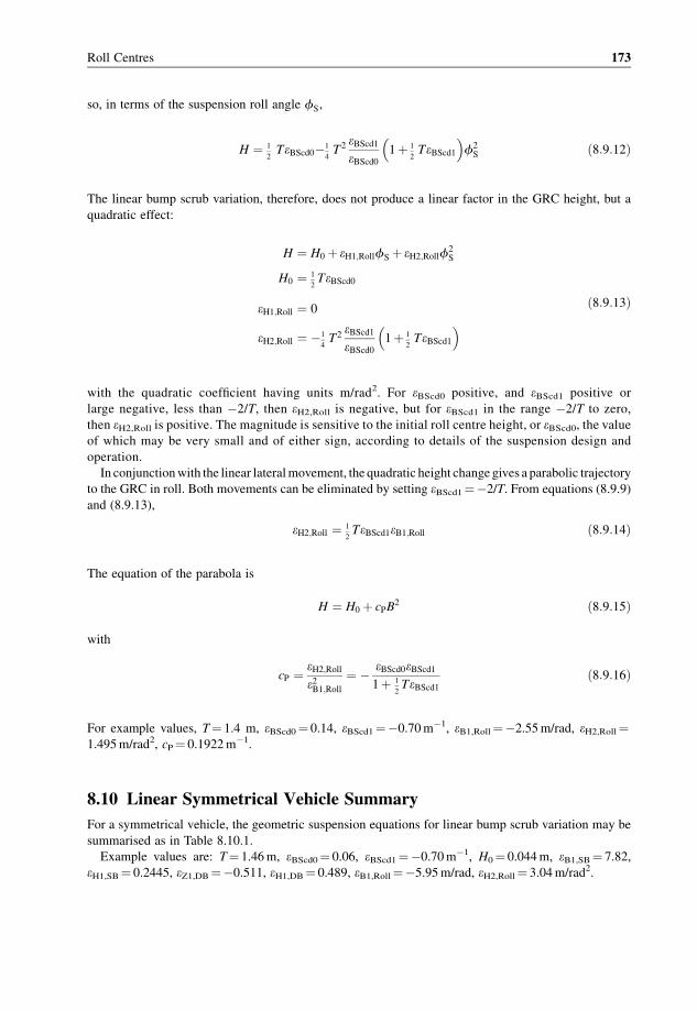
so, in terms of the suspension roll angle fS,

H ¼ 1

2TeBScd0�1

4T2 eBScd1

eBScd01þ 1

2TeBScd1

� �f2S ð8:9:12Þ

The linear bump scrub variation, therefore, does not produce a linear factor in the GRC height, but a

quadratic effect:

H ¼ H0 þ eH1;RollfS þ eH2;Rollf2S

H0 ¼ 1

2TeBScd0

eH1;Roll ¼ 0

eH2;Roll ¼ �1

4T2 eBScd1

eBScd0

�1þ 1

2TeBScd1

�ð8:9:13Þ

with the quadratic coefficient having units m/rad2. For eBScd0 positive, and eBScd1 positive or

large negative, less than �2/T, then eH2,Roll is negative, but for eBScd1 in the range �2/T to zero,

then eH2,Roll is positive. The magnitude is sensitive to the initial roll centre height, or eBScd0, the valueof which may be very small and of either sign, according to details of the suspension design and

operation.

In conjunctionwith the linear lateralmovement, the quadratic height changegives a parabolic trajectory

to the GRC in roll. Both movements can be eliminated by setting eBScd1¼�2/T. From equations (8.9.9)

and (8.9.13),

eH2;Roll ¼ 1

2TeBScd1eB1;Roll ð8:9:14Þ

The equation of the parabola is

H ¼ H0 þ cPB2 ð8:9:15Þ

with

cP ¼ eH2;Rolle2B1;Roll

¼ � eBScd0eBScd11þ 1

2TeBScd1

ð8:9:16Þ

For example values, T¼ 1.4 m, eBScd0¼ 0.14, eBScd1¼�0.70m�1, eB1,Roll¼�2.55m/rad, eH2,Roll¼1.495m/rad2, cP¼ 0.1922m�1.

8.10 Linear Symmetrical Vehicle Summary

For a symmetrical vehicle, the geometric suspension equations for linear bump scrub variation may be

summarised as in Table 8.10.1.

Example values are: T¼ 1.46m, eBScd0¼ 0.06, eBScd1¼�0.70m�1, H0¼ 0.044m, eB1,SB¼ 7.82,

eH1,SB¼ 0.2445, eZ1,DB¼�0.511, eH1,DB¼ 0.489, eB1,Roll¼�5.95m/rad, eH2,Roll¼ 3.04m/rad2.

Roll Centres 173

8.11 Roll of an Asymmetrical Vehicle

Figure 8.11.1 shows the geometry for movement of the GRC relative to the body when the asymmetrical-

suspension-geometry vehicle is rolledwith no heave. The small track variation is neglected. Vehicle bump

scrub asymmetry is now included, although this does not show in the diagram. The simultaneous equations

for B and H in general form are as in the previous section, and the solution is the same:

B ¼ �2zR þ 1

2TeBScd;L�R

eBScd;RþL

ð8:11:1Þ

Table 8.10.1 Summary of equations for symmetrical vehicle GRC

eBScd ¼ eBScd0 þ eBScd1zSB (8.10.1)

H0 ¼ 12TeBScd0 (8.10.2)

B0 ¼ 0 (8.10.3)

eB1;SB ¼ 12eBScd0

þ 12TeBScd1 (8.10.4)

eH1;SB ¼ 121þ 1

2TeBScd1Þ

�(8.10.5)

eB1;DB ¼ 0 (8.10.6)

eZ1;DB ¼ 12TeBScd1 (8.10.7)

eH1;DB ¼ 1þ 12TeBScd1 (8.10.8)

eB1;Roll ¼ � 12T

�1þ 1

2TeBScd1

�eBScd0 (8.10.9)

eH1;Roll ¼ 0 (8.10.10)

eH2;Roll ¼ � 14T2 eBScd1

eBScd0

� �1þ 1

2TeBScd1

� �(8.10.11)

Figure 8.11.1 An asymmetrical suspension geometry vehicle with rolled suspension, rear view, in vehicle

coordinates, but still with zero heave, the same diagram as Figure 8.9.1.


H ¼ zReBScd;L�R þ TeBScd;R�L

eBScd;RþL

ð8:11:2Þ

Now consider asymmetrical linear bump scrub variation (still with equal and opposite bumps, zL¼�zR):

eBScd;R ¼ eBScd0;R þ eBScd1;RzR

eBScd;L ¼ eBScd0;L � eBScd1;LzRð8:11:3Þ

with further relationships

eBScd;RþL ¼ eBScd0;RþL þ eBScd1;R�LzR

eBScd;R�L ¼ eBScd0;R�L þ eBScd1;RþLzRð8:11:4Þ

Inserting the linear variations into equation (8.10.1),

B ¼ �2zR � 1

2TeBScd0;R�L � 1

2TeBscd1;RþLzR

eBScd0;RþL þ eBScd1;R�LzRð8:11:5Þ

Taking the derivative of the quotient, and substituting zR¼ 0 gives the GRC lateral position variation in

roll as a function of the associated suspension bump deflection:

eB1;Roll;ZB ¼ �2eBScd0;RþL þ 1

2TðeBScd0;RþLeBScd1;RþL � eBScd0;R�LeBScd1;R�LÞ

e2BScd0;RþL

ð8:11:6Þ

This coefficient has units m/m, that is, no dimensions. To obtain this in terms of the actual roll angle, in

radians,

eB1;Roll ¼ 1

2TeB1;Roll;ZB ð8:11:7Þ

This has units m/rad, lateral motion of the GRC per radian of suspension roll angle.

8.12 Road Coordinates

The preceding analysis has been performed in the vehicle-body-fixed coordinates (B, H) because this is

much clearer than a suspension analysis in Earth-fixed road coordinates (Y, Z). However, for application,

it is desired to know the values in the Earth-fixed system, so a transformation of coordinates must be

applied, as seen in Figure 8.12.1. Thevehicle body position is defined by a heaveZB (a negative suspension

bump) followed by a suspension roll fS. The order of this sequence is significant; if the movement is

defined in the other order then the transformation equations are altered. Previous to the displacement, the

two axis systems (B, H) and (Y, Z) are coincident.

A general point P is at vehicle-fixed (B, H) and at Earth-fixed (Y, Z). By simple geometry,

Y ¼ B cosfS �H sin fS

Z ¼ B sin fS þ H cosfS þ ZBð8:12:1Þ

This may be arranged as two simultaneous equations in B andH, and solved by the usual methods, giving

B ¼ Y cos fS þðZ� ZBÞsin fS

H ¼ ðZ � ZBÞcos fS � Y sin fS

ð8:12:2Þ

The vehicle also heaves on the tyres because of changing total normal force and because of variation of

the effective tyre normal stiffness with lateral force, and the axle rolls on the tyres because of the lateral

transfer of normal force in cornering combined with the tyre vertical compliance. An additional

transformation, similar to the above, may be applied for this.

Roll Centres 175

When roll is applied before heave, the equations are

Y ¼ �ðH þ ZBfÞsin fS þ B cosfS

Z ¼ ðH þ ZBfÞcos fS þ B sin fS

ð8:12:3Þ

with

B ¼ Y cosfS þ Z sin fS

H ¼ �Y sin fS þ Z cosfS � ZBfð8:12:4Þ

Figure 8.12.2 shows the rolled vehicle, with swing arm angles in vehicle coordinates uSA,L and uSA,R.Relative to the road, the swing arm angles are

uSAR;L ¼ uSA;L �fS

uSAR;R ¼ uSA;R þ fS

ð8:12:5Þ

By this means, the GRC may be solved directly in road coordinates, if desired.

Figure 8.12.1 Vehicle-fixed (B,H) and Earth-fixed (Y, Z) coordinates: (a) with heave before roll; (b) with roll before

heave.

Figure 8.12.2 Rolled vehicle showing swing arm angles uSA in vehicle coordinates and uSAR in road coordinates.


The bump scrub rate coefficients may be expressed easily in road coordinates for small angles:

eBScdR;R ¼ eBScd;R þ fS

eBScdR;L ¼ eBScd;L � fS

ð8:12:6Þ

Using this method, all vehicles become asymmetrical.

8.13 GRC and Latac

For steady-state handling analysis, the roll centre height may be represented approximately by

H ¼ H0 þ kH1AY þ kH2A2Y

B ¼ B0 þ kB1AY þ kB2A2Y

ð8:13:1Þ

In a linear model, the suspension double bump (axle bump zA) and suspension roll angle fS are related

to the lateral acceleration (latac) by

zA ¼ kZAAY

fS ¼ kfSAY

ð8:13:2Þ

In simple roll, then, the GRC movements become

H ¼ H0 þ eH1;RollkfSAY þ eH2;Rollk2fSA2Y

B ¼ eB1;RollkfSAY þ eB2;Rollk2fSA2Y

ð8:13:3Þ

The linear effect on GRC height is usually quite small, being the result of vehicle asymmetries, so kH1 is

small. The coefficient kH2 is the quadratic roll-centre height variation coefficient, and again tends to be

small with a value possibly around plus or minus 0.001m/(m s�2)2 (0.1m/g2). In roll, kB1 may be around

�0.10 s2 [m/(m s�1)].

8.14 Experimental Roll Centres

Various methods have been suggested at times for the experimental measurement of roll-centre position,

none of which are really very satisfactory. One method is the observation of body displacement with

application of a lateral force at the centre of mass, for example using a laterally slanted ramp, but this is

definitely not suitable. The large lateral displacement at the tyres is a problemwhichmay be eliminated by

using solid wheels, but there will still be inappropriate lateral displacements within the suspension

compliances. A correct method of finding the SAE-defined roll centre would be to apply lateral forces

at various heights. With the lateral force applied at the height of the roll axis, there will be a lateral

displacement of the body because of compliances, and a vertical displacement because of the jacking

force, but no rotation. In this sense, the FRC is directly analogous to a shear centre, which would probably

be a better name for it, although the term ‘roll centre’ is no doubt too entrenched by use to change now.

As in the case of a shear centre, there is a more direct method of measurement. If the displacement is

observed when a moment is applied, the shear centre will be the centre of rotation, i.e. the point of zero

displacement. The most convenient way to apply a moment is by a couple, for example by a joist through

the doors, with a load first on one end then on the other. This does involve a vertical load which is

acceptable if the vehicle is to be tested in a loaded condition. Otherwise it is necessary to arrange for a

vertical upward force to be applied as half of the couple, say by a hydraulic jack or a weight over a pulley.

The actual deflection has been analysed by double-exposure photographs, but in the interests of accuracy it

is much better to take measurements of the displacement of specific points by dial gauges. If these points

Roll Centres 177

are not in the vertical transverse plane of thewheel centres, then the data must be used to find the roll axis,

and this then used to find the roll-axis position at each suspension.

This method is still subject to serious errors and problems. Under real cornering conditions there are

actually large forces in the suspension links, causing geometric changes through bush distortions. These

are largely absent from the test. Any small inappropriate lateral displacement of the body will give a large

error in the measured roll-centre height. The applied couple will change the load on the tyres, giving an

additional rotation of the complete chassis, including the wheels, about a point at ground level roughly

midway between the tyres. The result is a false lateralmotion of the body at roll centre height. Thismust be

guarded against by using solid disc wheels, although this exacerbates the problem of allowing scrub,

because when finding the roll centre for large angular displacements, there will be a consequent track

change. This must be permitted, perhaps with air bearing pads, but without allowing any inappropriate

lateral motion of the body, which is critical. It is difficult to say how the body should be located.

In summary, it is fairly easy to observe the displacement of a vehicle when it is subject to loads or

couples, but it is verymuchmore difficult to obtain results that have aworthwhile roll centre interpretation,

especially for large latacs. Probably the only satisfactory experimental method is to use an instrumented

vehicle in real cornering to find the displacements and actual load transfer for each axle, for examplewith

strain gauges on the links, and to deduce the KRC from the lateral displacements, and the net link load

transfer and FRC height from the forces.

References

Dixon, J.C. (1991) Tyres, Suspension and Handling, 1st edition. Cambridge: Cambridge University Press.

Dixon, J.C. (1996) Tires, Suspension and Handling, 2nd edition. London: Edward Arnold.

Analysis of the GRC using a variable bump scrub rate does not seem to have been published previously in any books

or research literature.

————— // —————


9

Compliance Steer

9.1 Introduction

This chapter discusses compliance steer effects in general terms. Specific designs of suspension are

covered in later chapters.

The wheel position, for a given suspension bump, is determined initially by the basic geometry of the

suspension, but this is modified by the forces and moments acting on the wheel, which cause compliance

deflections. These are generally small, but never zero. Theymay be a problem, with inadequate design, or

may be kept small or put to good effect by good design. For example, sometimes rear compliance oversteer

is deliberately introduced. Under tractive or braking forces, there may also be compliant changes of front

caster angle. These will augment the caster change relative to the ground caused by vehicle pitch due to

longitudinal load transfer.

In general, the compliance may be in the suspension or in the steering linkage. The main effects are

changes of wheel angles, known as compliance steer angles (dC) and compliance camber angles (gC). Thefundamental units are radians, and these are the units normally used in equations and computer programs,

but the usual form for human consumption is degrees.

For the design of ordinary passenger vehicles, handlingmust be seen in the context of the ride–handling

compromise. To provide comfort and to avoid noise, vibration and harshness, it is necessary to have

significant compliance of wheel motion, not just vertically but also in longitudinal and lateral directions,

achieved by tyre compliance, by the springs and by the extensive use of rubber bushes. Unfortunately,

suspension link compliance has often led to considerable angular compliance of the wheels, resulting in

unfavourable or unpredictable handling because of compliance camber deflection and especially because

of compliance steer deflection. Through better understanding, this conflict is now largely resolvable, by

allowing the wheel relatively generous movement in translation, but little angular movement in steer or

camber for the forces and moments that it actually experiences. The method is to bring the shear centre of

an independent suspension, in plan view, close to the centre of tyre contact, or for a rigid axle near to the

mid-point between the tyres. Tyre forces then have little moment about the shear centre, and so, although

the wheel still has angular compliance, there is little angular response, so that steer angle changes are

controlled. Careful location of the shear centre can even be used to introduce favourable small deflections.

A significant characteristic of compliance steer is that, unlike roll steer, it occurs almost immediately.

On low-friction surfaces such as ice or snow, the tyre characteristics are different, and there is a low limit

to lateral acceleration, so load transfer distribution becomes less significant, and roll steer and side-force

steer become more critical in determining limit handling, especially at the rear.


9.2 Wheel Forces and Moments

The basic coordinate system for the wheel is shown in Figures 9.2.1 and 9.2.2. At the base of the wheel, at

the notional centre of the undistorted contact patch, there are three forces and threemoments acting on the

wheel, Figures 9.2.3 and 9.2.4.More accurately, one should say that there is one resultant wrench,which is

a force with a coaxial moment, which may usefully be considered in terms of these six components.

The origin of the wheel coordinate system is the intersection of the ground plane, the undistorted wheel

Figure 9.2.2 The SAE coordinate system for a wheel (SAE, 1976).

Figure 9.2.1 The ISO coordinate system for a wheel.


plane and the transverse vertical plane through the wheel centre. The axis directions are:

(1) the X axis, forward in the ground and wheel planes;

(2) the Y axis, in the ground and transverse vertical planes;

(3) the Z axis, perpendicular to the ground in the transverse plane.

Note that the Z axis is not in the wheel plane, unless the wheel has zero inclination.

Figure 9.2.4 The total wrench at the base of a wheel, exerted by the ground on the wheel, analysed as six

force–moment components, SAE system.

Figure 9.2.3 The total wrench at the base of a wheel, exerted by the ground on the wheel, analysed as six

force–moment components, ISO system.

Compliance Steer 181

9.3 Compliance Angles

Apart from the ride-improving properties of the suspension compliance, the most important compliance

effects are those directly affecting the handling qualities, specifically the compliance steer angle and the

compliance camber angle or compliance inclination angle, Figure 9.3.1. Considering these angles, for a

given design of suspension location system with its rubber bushes, reveals the critical aspects of the

suspension in this regard. The steer angles are measured from a line parallel to the vehicle centreline, with

a total steer angle which is simply the sum of the geometric and compliance angles:

d ¼ dG þ dC ð9:3:1ÞSimilarly, the inclination or camber angles may be measured from the perpendicular to the road surface,

with

g ¼ gG þ gC ð9:3:2ÞAlso, for pitch angle (caster angle) of the wheel hub,

u ¼ uG þ uC ð9:3:3ÞThe pitch angle variation changes the caster angle of the wheel upright. With positive rotation as right-

hand about the Y-axis, the static caster angle would be negative, so this sign convention is rarely applied.

Figure 9.3.1(c) shows positive values of uG and uC, caster being simply taken as positivewhen the steering

axis leans backwards.. Thewheel hub pitch angle is not necessarily identical to the caster angle, the former

possibly being defined as zero in the static position, although the difference will be constant at the static

caster minus static hub pitch angle.

9.4 Independent Suspension Compliance

The total force and moment wrench at each independent wheel contact patch is considered as three force

and three moment components: FX, FY, FZ, MX, MY, MZ. Also there are six possible displacement

responses of the wheel: X, Y, Z, g, u, d. Each displacement response may be affected by each of the six

stimuli, so, considering even the simplest linear model, there will be 36 coefficients in total. This can be

Figure 9.3.1 Compliance steer and compliance inclination angles for a single wheel: (a) steer angle in plan view; (b)

inclination angle in rear view; (c) hub pitch angle in side view.


combined into a matrix equation

X ¼ CF ð9:4:1Þ

where X is the six-component linear and angular compliance displacement column vector

X ¼ ðXC; YC; ZC; gC; uC; dCÞT ð9:4:2Þ

in which the suffix T means transpose (in this case, just change the row to a column); F is the six-

component force–moment column vector,

F ¼ ðFX;FY;FZ;MX;MY;MZÞT ð9:4:3Þ

and C is the compliance matrix. This matrix equation has no special properties, it is just a simple and

concise way of writing the combined linear equations. In more detail

XC

YC

ZC

gCuCdC

0BBBBBBB@

1CCCCCCCA

¼

CX;FX CX;FY CX;FZ CX;MX CX;MY CX;MZ

CY;FX CY;FY CY;FZ CY;MX CY;MY CY;MZ

CZ;FX CZ;FY CZ;FZ CZ;MX CZ;MY CZ;MZ

Cg;FX Cg;FY Cg;FZ Cg;MX Cg;MY Cg;MZ

C u;FX C u;FY C u;FZ C u;MX C u;MY C u;MZ

Cd;FX Cd;FY Cd;FZ Cd;MX Cd;MY Cd;MZ

0BBBBBBB@

1CCCCCCCA

�

FX

FY

FZ

MX

MY

MZ

0BBBBBBB@

1CCCCCCCA

ð9:4:4Þ

This is simply, then, a concise way of representing six equations of the form

XC ¼ CX;FXFX þ CX;FYFY þ CX;FZFZ þ CX;MXMX þ CX;MYMY þ CX;MZMZ ð9:4:5ÞThe units of the compliance matrix are in four equal 3� 3 sections:

units ðCÞ ¼ m=N m=Nm ¼ N�1

rad=N rad=Nm

� �

Fortunately, in view of the large number of coefficients at each wheel, many of the effects are

insignificant in practice. This occurs if the stimulus is small, if the compliance is small, or if the resulting

deflection is unimportant. Expressed in partial derivatives, the more interesting and important com-

pliances of the matrix are as follows:

C ¼

qXqFX

� � � qXqMY

�

� qYqFY

� � � �

� qZqFY

qZqFZ

� qZqMY

�

� qgqFY

qgqFZ

qgqMX

� �

q uqFX

� � � q uqMY

�

qdqFX

qdqFY

qdqFZ

qdqMX

qdqMY

qdqMZ

26666666666666666666666664

37777777777777777777777775

ð9:4:6Þ


Here it is apparent that the rows are the various coefficients for the effects on one displacement

(e.g. the sixth row is for changes to the wheel steer angle d), and columns are the coefficients for the

effects of a given force or moment (e.g. the second column is for the effects of FY, the lateral force).

The values in this matrix are normally positive, but this is contingent upon the sign conventions

adopted. A matrix of derivatives such as this is known mathematically as a Jacobean matrix (with

emphasis on the ‘oh’).

9.5 Discussion of Matrix

To understand the terms of the Jacobean sensitivity matrix, it is necessary to define clearly the conditions

of the partial derivatives. Basically, the body is held fixed, and the wheel is initially held at its normal

position by a vertical force, which would normally support the vehicle. The wheel is locked to the hub

in rotation. Additional forces and moments are then applied and the displacements are measured. The

meaning and significance of the results are not always completely obvious, and the results require

interpretation. For example, as tested with a wheel and tyre, the lateral displacement response to a lateral

force shows a large value due to the tyre lateral compliance. Normally, this would be treated separately,

so the tyre compliance would be excluded from the compliance matrix, leaving only the structural

compliance. Similarly, the vertical displacement response to vertical force is dominated by the suspension

spring compliance and tyre vertical compliance, which would be deducted to leave the structural

compliance only. In the case of formula racing cars with long wishbones, this may be important.

In some applications of the compliance matrix, the compliances of the spring, etc., may be included.

This is just amatter ofmethodology, but it is important to be clear what thematrix compliances do include

in any particular case.

In the first row, X displacements, sensitivity to FX is deliberately introduced by appropriate rubber

bushes. This is to prevent a significant harshness on hitting bumps. Bias-ply tyres (diagonal-ply) are

more compliant, but with the widespread use of radial-ply tyres which are much less compliant in the

longitudinal direction it is really essential to make appropriate use of this suspension compliance in

modern road vehicles. Exceptions are, naturally, off-road vehicles which generally use diagonal-ply tyres

because these have sidewalls of greater strength. Sensitivity of X to MY is of interest because it relates

sensitivity towheel contact-patch height forces to the sensitivity to axle-height forces. Thesemoments are

produced by variations in rolling resistance and by traction or braking forces produced through the action

of a driveshaft.

The second row has an entry for qY/qFY, the lateral compliance. This is generally not important, not

least because the tyre itself exhibits a larger lateral compliance, whichwould normally be eliminated from

an experimental measure, but it is easy to see physically how the residual lateral structural compliance at

the contact patch arises from linear lateral compliance of two wishbones.

In the third row, qZ/qFY is the change of vertical position with lateral force. This may appear to be the

suspension link jacking effect, but usually this would be separated out and dealt with as an independent

item, not classified as compliance. Link jacking can occur evenwith ideally-rigid links. The residual term

is small and due to link compliance only, allowing a small verticalmotion of thewheelwith the body fixed.

The next entry in the third row is qZ/qFZ, the change of vertical position with vertical force. This is the

main suspension action, and again this would normally be separated out and dealt with by other means.

The basic compliance here is the large ride compliance, the sum of the spring (wheel rate) and tyre normal

compliances:

CR ¼ 1

KS

þ 1

KZT

ð9:5:1Þ

The matrix compliance coefficient here, CZ,FZ, would normally apply to any additional deflection, above

that due to the spring and tyre action, due to distortion of the links and deflection of rubber bushes.


The third term shown in the third row is qZ/qMY, which is the effect of pitching moment on vertical

position. This is mentioned because such an effect can arise in the case of trailing arms, but is then

analogous to link jacking, and, similarly, would be dealt with separately.

In the fourth row, the effects on inclination/camber angle, significant effects are shown for FY, FZ and

MX. The way in which these can alter a camber angle through compliance of the links is easy to imagine.

The fifth row, for changes of pitch angle, has two entries. The pitch angle of the wheel is not a handling

or ride issue, because thewheel rotates anyway, but the pitch angle should be considered to be the angle of

the wheel hub. This can deflect in pitch compliance due to pitch moments or longitudinal forces from

traction or braking, changing the steering caster angle.

The sixth row, that for steer angle effects, which is most critical, is full, although in practice some of

these terms are small. The first term, qd/qFX, is the important steer effect of tractive and braking forces.

The second term, qd/qFZ, is the important steer effect of lateral forces. The third term, qd/qFY, is the steer

effect of vertical forces. The fourth term, qd/qMX, is the steer effect of the tyre overturning moment,

usually small. The fifth term, qd/qMY, is the steer effect of pitch moment. The final term, qd/qMZ, is the

steer effect of wheel yaw moments (e.g. due to mechanical or pneumatic trail combined with lateral

forces), and may be significant.

9.6 Independent-Suspension Summary

The main structural compliance effect in ride is:

(1) CX,FX (m/N), the longitudinal compliance to longitudinal force.

For formula racing cars, the structural vertical compliance to vertical force may be as great as the basic

spring compliance, because of the use of stiff suspensions but long thin links and body compliance at the

connection points.

The main structural compliance effects in handling are:

(1) Cd,FY (deg/N), the lateral force compliance steer coefficient;

(2) Cd,MZ (deg/Nm), the aligning moment compliance steer coefficient;

(3) Cg,FY (deg/N), the lateral force compliance camber coefficient;

(4) Cg,MX (deg/Nm), the overturning moment compliance camber coefficient.

The last of these is usually neglected, and often the last two or three. The actual compliance steer angle is

typically expressed as

dC ¼ dFY þ dMZ ¼ Cd;FYFY þ Cd;MZMZ ð9:6:1Þ

and the compliance inclination angle is

gC ¼ gFY þ gMX ¼ Cg;FYFY þ Cg;MXMX ð9:6:2Þ

In the case of compliance camber, some symbol other than gmight be desirable, but there is no commonly

accepted symbol. The use of g is acceptable provided that the corresponding preference for d rather thanais clearly understood in the case of compliance steer.

The total effect of compliance in the linear cornering regime may be summarised by the compliance

steer gradient kdC, which has SI units rad/m.s–2, but is usually expressed in deg/g. Because the lateral

force effective in creating distortions is the sprung mass force rather than the total lateral force, the


compliance gradients are as follows:

kd;C ¼ kd;FY þ kd;MZ

kd;FY ¼ mBfCd;FY;f þmBrCd;FY;r

kd;MZ ¼ mBftfCd;MZ;f þmBrtrCd;MZ;r

ð9:6:3Þ

where mB is the body mass (sprung mass) and t is the tyre pneumatic trail. Similar equations can

be written for the camber. Typical values of compliance understeer gradient are 1.0 deg/g at the front and

0.2 deg/g at the rear.

9.7 Hub Centre Forces

For a driven wheel, or with inboard brakes, the driveshaft transmits a moment MD which, for constant

wheel angular speed, generates a longitudinal force

FX ¼ MD

RL

ð9:7:1Þ

where RL is the loaded radius of the wheel. As shown in Figure 9.7.1, this combination of force and

moment is equivalent to a force only, atwheel centre height. It is also equivalent to a forceFX at the contact

patch plus a pitching momentMY there, whereMY¼MD. Comparing Figure 9.7.1(a) and (c), the moment

has been moved. This is permissible, as the application point, or axis, of a moment has no effect on the

influence of the moment on a rigid body. The configuration of Figure 9.7.1(c) can then be used with the

compliance matrix to obtain the compliance deflections for the hub-height force. This illustrates the

principle, although, of course, in a practical case there may be complications; for example, with an

inclined driveshaft there will be an additional moment MZ.

It is also of interest to obtain the coefficients for the force FX applied directly at the wheel centre. The

compliance steer angle is

dC ¼ Cd;FXFX þCd;MYFXRL ð9:7:2Þ

so the compliance steer coefficient for the wheel-centre-height force is

Cd;FX;WCH ¼ Cd;FX þCd;MYRL ð9:7:3Þ

This may be elaborated to include other effects such as an inclined driveshaft. Similar methods may be

applied to other coefficients.

Figure 9.7.1 Equivalent force systems for tractive force generated by driveshaft torque.


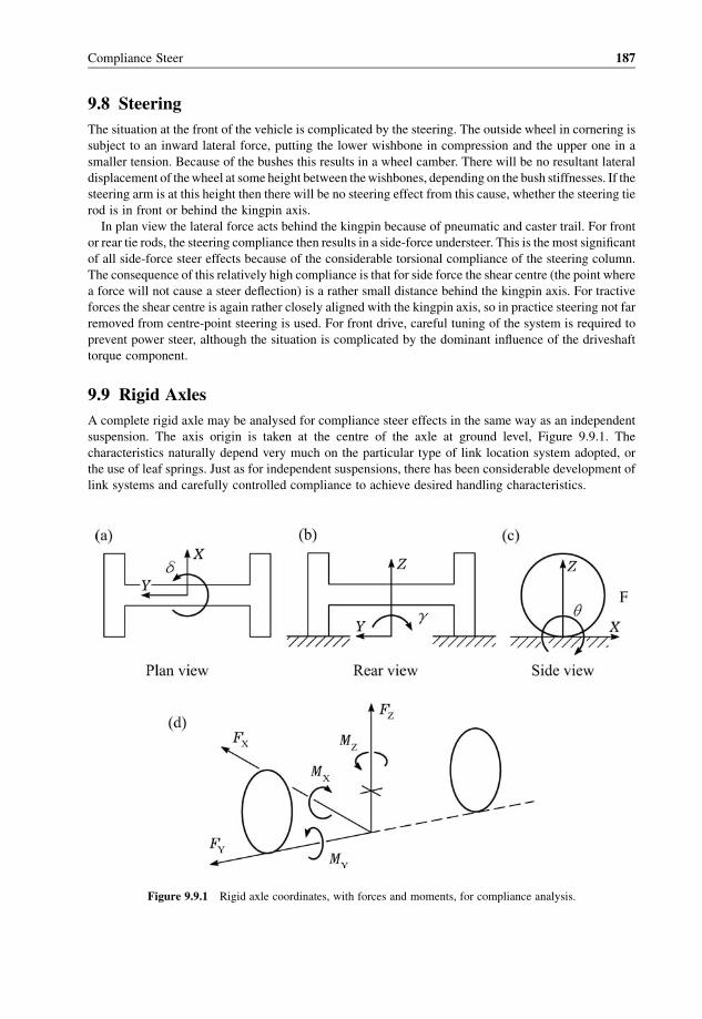
9.8 Steering

The situation at the front of the vehicle is complicated by the steering. The outside wheel in cornering is

subject to an inward lateral force, putting the lower wishbone in compression and the upper one in a

smaller tension. Because of the bushes this results in a wheel camber. There will be no resultant lateral

displacement of thewheel at some height between thewishbones, depending on the bush stiffnesses. If the

steering arm is at this height then there will be no steering effect from this cause, whether the steering tie

rod is in front or behind the kingpin axis.

In plan view the lateral force acts behind the kingpin because of pneumatic and caster trail. For front

or rear tie rods, the steering compliance then results in a side-force understeer. This is the most significant

of all side-force steer effects because of the considerable torsional compliance of the steering column.

The consequence of this relatively high compliance is that for side force the shear centre (the point where

a force will not cause a steer deflection) is a rather small distance behind the kingpin axis. For tractive

forces the shear centre is again rather closely aligned with the kingpin axis, so in practice steering not far

removed from centre-point steering is used. For front drive, careful tuning of the system is required to

prevent power steer, although the situation is complicated by the dominant influence of the driveshaft

torque component.

9.9 Rigid Axles

A complete rigid axle may be analysed for compliance steer effects in the same way as an independent

suspension. The axis origin is taken at the centre of the axle at ground level, Figure 9.9.1. The

characteristics naturally depend very much on the particular type of link location system adopted, or

the use of leaf springs. Just as for independent suspensions, there has been considerable development of

link systems and carefully controlled compliance to achieve desired handling characteristics.

Figure 9.9.1 Rigid axle coordinates, with forces and moments, for compliance analysis.


9.10 Experimental Measurements

Various rigs have been built for the measurement of suspension compliance, typically combined with

measurement of geometric bump steer and bump camber. Basically, such a rig comprises a rigid frame

replacement of the vehicle body, to which the suspension arms are connected in the usual way. Hydraulic

actuators apply forces or moments in the desired way, with deflection measurements made by dial gauges

or some automated system. By this means the linear coefficients can be determined, along with non-linear

effects and the limits of linearity. Usually, the suspension spring is replaced by a rigid link, and thewheel is

replaced by a rigid disc or structure, to isolate the structural compliances. The wheel compliance,

excluding the tyre, can be tested separately, and is relatively small.

References

SAE (1976) Vehicle Dynamics Technology, SAE J670e. Warrendale, PA: Society of Automotive Engineers (reprinted

as an appendix to J.C. Dixon (1996) Tires, Suspension and Handling, 2nd edition. London: Edward Arnold).

————— // —————


10

Pitch Geometry

10.1 Introduction

Vehicle longitudinal dynamics dictate certain aspects of suspension geometry. As a result of aerodynamic

pitching moment, hill climbing, braking or accelerating, or steady-state cornering with an attitude angle,

there is a longitudinal load transfer, that is, longitudinal transfer of tyre vertical force. It is considered

positive when the rear reactions are increased. The change of vertical force in the suspension results in

ride-height changes at the front and rear suspensions. The suspension bump deflections have geometric

effects on thewheels, such as bump camber and bump steer angle changes, and also affect the caster angles

significantly. As in the case of lateral load transfer, the longitudinal load transfer may be achieved partly

through the springs and partly through the links. Transfer of some of the load through the links rather than

through the springs is called ‘anti-dive’ at the front and ‘anti-rise’ at the rear in the case of braking, and

‘anti-lift’ at the front and ‘anti-squat’ at the rear in the case of traction. Having a roll centre above ground

could correspondingly be described as ‘anti-roll’. These all depend on the geometry of the suspension

links.

10.2 Acceleration and Braking

The total longitudinal load transfer moment reacted by the tyres at a longitudinal acceleration Ax, for a

total vehicle mass m and centre-of-mass height H, is

MTXT ¼ mHAx

Similar additional effects occur for a longitudinally sloping road. The basic load transfer moment on the

suspension is due to the sprung mass:

MTXS ¼ mSHSAx

However, the unsprung mass contributes to the longitudinal load transfer, and part of this acts through the

sprung mass, having some effect on the pitch angle, again depending on details of the suspension

geometry. Therefore the second equation above is not strictly correct. Also, of course, the pitch angle

resulting from tyre deflections depends on the entire load transfer.

The pitch stiffness (as Nm/rad) of the tyres along the wheelbase, with the vehicle pitching about its

centre of mass, is

kTP ¼ 2a2Ktf þ 2b2Ktr


whereKt is the tyre vertical stiffness (onewheel) and a and b are the partialwheelbases, and twowheels per

axle are assumed. This gives an unsprung-mass pitch angle (i.e. the pitch angle of the line through the

wheel centres in side view) of

uU ¼ mSHSAx

kTP

The suspension pitch stiffness (Nm/rad) is

kSP ¼ 2a2KSf þ 2b2KSr

where KS is the effective suspension vertical stiffness at one wheel, giving a suspension pitch angle, with

no anti-dive or anti-rise effect, of

uS ¼ mSHSAx

kSP

The complete body pitch angle, for steady acceleration, is the total pitch angle on the tyres and suspension:

uB ¼ uU þ uS

with an associated pitch angle gradient du=dAx around 4 deg/g (longitudinal).

10.3 Anti-Dive

Really the whole suspension is a geometric problem to be solved in three dimensions, as in later chapters,

but for human understanding it is useful to consider approximate two-dimensional simplifications. The

principle of anti-dive for a twin-wishbone front suspension is shown in two-dimensional side view in

Figure 10.3.1. Each wishbone has a geometric plane through three points (e.g. two on the body plus one at

the centre of the ball joint on thewheel upright). There is a linewhere the plane of eachwishbone intersects

the longitudinal plane of the wheel, these lines being shown in the figure. These two lines are arranged to

converge to a point E, possibly at infinity. The line AE at angle ugf (gf for ground front) joins this point to

the base of thewheel. The suspension geometry is characterised primarily by the angle ugf and by the pitcharm length LAE or the horizontal pitch arm radius LAD.With the usual approximation of zero stiffness and

friction moment about the pivot axis, the suspension links can exert no moment about the point E. When,

resulting from brake action, a horizontal force is applied by the road to thewheel at the bottom, this can be

resolved into components along and perpendicular to the line AE. The component F1 along AE is reacted

by the links. The component F2 perpendicular to AE must be reacted by the springs: at the front a

Figure 10.3.1 Anti-dive and anti-squat geometry (only braking forces shown).


component of the braking force acts downwards on the wheel, extending the spring and so opposing the

usual compression of the front spring in braking. This is anti-dive.

Figure 10.3.1 assumes that the brakes are outboard. If they are inboard then the torque transferred by the

driveshafts must be added to the brake force. The result is that the brake force is effectively applied at the

wheel centre height, so it is necessary to arrange for appropriate inclination of line CE instead. Similar

principles can be applied to the rear suspension, but in this case the force centre must be in front of the

wheel, to discourage the usual extension of the rear springs in braking or compression in acceleration.

The pitch properties of the suspension therefore depend on the position of the point E, and so on the

suspension geometry.

The notation for angles in Figure 10.3.1 is that subscripts c and g mean from the centre and ground

respectively, and subscripts f and r mean front and rear as usual. The anti coefficients will be

denoted by J (in practice often expressed as J� 100%). For example, JAL is the anti-lift coefficient.

Table 10.3.1 summarises the parameters, showing which angle is relevant to which coefficient. As an

aide-m�emoire to distinguish between rise and lift, it is convenient to recall that rise is at the rear.

Inboard brakes are relatively rare, being used on a few high-performance vehicles and some racing cars.

Outboard drive is very unusual, achieved on some specialist vehicles by hydraulic or electrical drive, in

which case there is no driveshaft torque, analogous to conventional brakes.

In braking, the total deceleration depends on the total longitudinal tyre force from the two ends of the

vehicle, but the horizontal longitudinal suspension force on each end depends on the braking proportion at

that end. Accurate calculation of the anti-dive coefficient requires consideration of the proportion of brake

force at the front, the sprung and unsprung masses, and the sprung centre-of-mass height. The analysis is

usually simplified by neglecting the inertial effect of the unsprung mass, as in the following. As an

example, consider the braking force

F ¼ Ff þFr ¼ pmAB þð1� pÞmAB

where p is the proportion of braking at the front, which may be acceleration-dependent, for example if

there is a rear pressure limiter, and AB is a braking deceleration, positive to the rear. The resulting vehicle

deceleration is

AB ¼ Ff þFr

m

The total longitudinal transfer of vertical tyre force to the rear is

FTX ¼ �mABH

L

Table 10.3.1 Anti-dive/rise/lift/squat coefficients and angles

Action Symbol Direction End Relevant angle

Inboard brake/drive Outboard brake/drive

Anti-dive JAD braking front ucf ugfAnti-rise JAR braking rear ucr ugrAnti-lift JAL driving front ucf ugfAnti-squat JAS driving rear ucr ugr

Pitch Geometry 191

The vertical force exerted by the ground on the front axle is therefore

FVf ¼ Wf �FTX ¼ Wf þ mABH

L

The forces on the suspension from the body have no moment about E, so taking moments about E for the

front wheel shows the effective front spring force (sum of two wheels) to be approximately

FS ¼ Wf �WUf þ mABH

L� pmABy

x

Hence the front anti-dive against forces exerted on the wheel at ground level (e.g. for outboard brakes) is

Jgf ¼ pðy=xÞH=L

¼ tan ugftan ugfi

where ugfi is the ‘ideal’ angle for full anti-dive, given by

tan ugfi ¼ H

pL

10.4 Anti-Rise

In braking, with outboard brakes, at the rear the anti-rise is correspondingly given by

Jgr ¼ tan ugrtan ugri

where

tan ugri ¼ H

ð1�pÞL

is the full anti-rise angle.

10.5 Anti-Lift

In the case of traction, with tractive force

F ¼ Ff þFr ¼ tmAx þð1� tÞmAx

where t is the tractive force fraction on the front wheels, the tractive force is produced because of torque in

the driveshafts, totalling for both wheels tmAr at the front and (1� t)mAr at the rear, neglecting rotational

inertia of the wheels. This means that the effective line of action of the tractive force is transferred to the

centre of the wheel. The front anti-lift is

Jcf ¼ t½ðy� rÞ=x�H=L

¼ tan ucftan ucfi

where ucf is the angle of the line CE at the front:

tan ucf ¼ y� r

x


and ucfi is the angle for full anti-lift, given by

tan ucfi ¼ H

tL

10.6 Anti-Squat

The traction anti-squat at the rear is

Jcr ¼ ð1� tÞ½ðy� rÞ=x�H=L

¼ tan ucrtan ucri

where the full anti-squat angle is

tan ucri ¼ H

ð1� tÞL

In the case of inboard brakes, the braking force is associated with a driveshaft torque, so the inclination of

line CE gives the relevant angle. All the above equations can be extended to include the effect of the

translational and rotational inertia of the unsprung masses. For example, during linear vehicle decelera-

tion, thewheels also have angular deceleration, with angular momentum change that must be provided by

the moment of a longitudinal load transfer.

10.7 Design Implications

In practice there are objections to anti-dive geometry. It tends to cause harshness of the front suspension

on rough roads because the wheel moves forward as it rises, attacking the bump; it may also cause

steering kick-back and wander under braking. It also becomes more difficult to achieve good-quality

steering geometry, so instead of full anti-dive a proportion is often used, usually expressed as a

percentage. Up to 50% anti-dive has been used on passenger cars. Amounts in excess of 50% have been

used on ground-effect racing cars because of their extreme sensitivity to pitch angle. However, a large

amount may be problematic on small-radius turns, where the large steer angle plus cornering force

results in significant jacking forces. The most successful applications of anti-dive seem to be those in

which the geometry is arranged to minimise changes of caster angle, and the anti-dive quantity is more

moderate at 20% to 25%.

Considering again Figure 10.3.1, characterised by the angle ugf and horizontal anti-dive arm radiusLAD,

it is apparent that vertical motion of the wheel (i.e. suspension bump) will give an effective rotation about

some point. In the case of a rigid leading arm, this point is simply the body-fixed point E.Any such rotation

changes the effective angle of motion ugf so the anti-dive coefficient will vary significantly with the

suspension bump position. The pitch angle of the body, perhaps 4–5� in strong braking, will also influenceugf. Any effective rotation also changes the caster angle relative to the body; this can be eliminated, if

desired, by using parallel arms, although this still leaves the body pitch angle affecting the caster angle,

that is, the anti-dive and the geometric caster change can be chosen independently.

From Section 5.10, the caster angle relative to the ground, expressed as a linear model equation, is

uC ¼ uC0� uB þ «BCaszSf

where uC0 is the static caster angle, uB is the body pitch angle (positive nose down), and «BCas is the bump

caster coefficient. The possibility exists ofmaintaining uC constant by using the bump caster coefficient to

counteract the effect of the body pitch angle.

Pitch Geometry 193

The bump caster coefficient is

«BCas ¼ 1

LAD

which is the reciprocal of the pitch arm radius. The front and rear suspensions are of approximately equal

stiffness, so the front suspension bump is

zSf ¼ 1

2LW uB

where LW is the wheelbase. The bump caster angle is then

uBCas ¼ «BCaszSf ¼ «BCas1

2LW uB

To fully offset the body pitch angle effect,

uBCas� uB ¼ 0

so requiring

«BCas ¼ 2

LW

Considered evenmore simply, the vehicle pitches roughly about itsmid-wheelbase position, so if the point

E is atmid-wheelbase then the caster angle relative to the roadwill not be affected. Thereforewe desire the

pitch arm radius LAD to be LW/2. This simple analysis can easily be made more accurate for particular

cases by calculation of the actual pitch angle and suspension bump values.

In the case of the pitch-up caused by traction forces, with rear-wheel drive it is quite common to have

some anti-squat at the rear. It is not possible to provide anti-rise at the front of a rear-wheel-drive vehicle

because there is no associated horizontal force applied to the wheel. Anti-squat may have detrimental

effects on traction on rough surfaces. Anti-squat effectsmay also be achieved by other arrangements of the

rear suspension, such as a lift bar, which is rigidly attached to the rear axle, protruding forward and acting

upward on a rubber block on the body; the axle reaction torque therefore provides an upward force on the

rear body, depending on the length of the lift bar, relieving the rear springs.

Having chosen desired ‘anti’ coefficients, at least a partial geometric specification for the suspension

side view can be made.

For the front suspension, the anti-dive gives ugf. If thevehicle is front-wheel drive, then the anti-lift givesucf and the point E is thereby determined for the front. For the front suspensionwith rear-wheel drive, ucf isunspecified, and the length of the anti-squat arm could be chosen freely, possibly infinite, or on other

criteria, such as the caster angle effect as described above.

For the rear suspension with rear-wheel drive, the required anti-rise and rear-wheel-drive anti-squat

together specify E. For the rear suspension of front-wheel drive, only the anti-rise is relevant, and then the

arm length may be freely chosen.

The preceding simplified description and analysis of longitudinal behaviour is based on approximate

two-dimensional considerations to convey the principle. A more complete quantitative analysis requires

consideration of the suspension in three dimensions, as in later chapters.

————— // —————


11

Single-Arm Suspensions

11.1 Introduction

This chapter dealswith suspensions inwhich thewheel hub is located by a single rigid arm (various type of

trailing arm, swing axles, etc.). The alternatives, in later chapters, are to use location by two arms, as for

doublewishbones, or by onewishbone and a trunnion, as on struts, and some other types. Pictures ofmany

examples of these various types of suspension appear in Chapter 1.

Considering rigid single-arm suspensions, then, there are two rotational axes to consider, the wheel

rotation axis and the arm pivot axis. The wheel rotation axis is fixed relative to a single arm, which is

pivoted on the vehicle body. For a single-arm suspension, this pivot axis is fixed relative to the body. The

fixity of this axis is a distinctive feature fromother suspensions inwhich the pivot axis is virtual andmoves

relative to the members and the body. A fixed position of the axis generally simplifies the analysis, and

certainly changes the details of the methods of solution.

These are all independent suspensions, so the geometric steer effects are expressed in basic form by the

bump coefficients (bump camber, bump steer, etc.). In general, a slope angle of the pivot axis, out of the

horizontal plane, introduces linear bump steer. A sweep angle, in plan view, affects the quadratic bump

steer coefficient. Camber coefficients are also affected. The small static wheel toe and camber angles also

interact with the axis angles to give some bump steer and camber effects, not always negligible. The pivot

axis height also introduces small steer effects in some cases. In general, then, it is necessary to investigate

the effect of:

(1) the pivot axis plan-view sweep angle cAx;

(2) the pivot axis slope angle (out-of-horizontal) fAx;

(3) the pivot axis height HAx;

(4) the wheel static toe angle d0;(5) the wheel static camber angle g0.

These may influence, in the present context:

(1) the bump steer coefficients «BS1 and «BS2;

(2) the bump camber coefficients «BC1 and «BC2;(3) the bump scrub rate coefficient «BScd0 (roll centre height);

(4) the bump scrub rate variation coefficient «BScd1 (roll centre movement).


For the occasional cases of a rigid arm with steering, additional factors are:

(5) the bump kingpin inclination angle coefficients «BKI1 and «BKI2;(6) the bump kingpin caster angle coefficients «BKC1 and «BKC2.

For the bump steer, for example, various mathematical models may be adopted, depending on the

purpose of the analysis. The main models are:

(1) exact analytical geometric model;

(2) approximate geometric model;

(3) linear bump steer coefficient;

(4) quadratic model (linear and quadratic bump steer coefficients);

(5) polynomial bump steer expression;

(6) accurate numerical (computer) solution.

Exact geometric models are sometimes useful, but require some skill to achieve, and are, except for

the very simple cases, rather unwieldy for most purposes. They have the advantage of being accurate

if correctly solved, but do not necessarily provide good insight because of the complexity of the ultimate

algebraic expression.

Approximate geometric models are simple to use, and are usefully close to correct over the practical

range of application.

Linear bump steer coefficients, usually derived from simplified geometric models, have been widely

used for many years. These, naturally, give considerable insight to linear bump steer effects, but omit the

second-order effects.

The quadratic bump steer expressions, including linear and second-order terms (the first and second

bump steer coefficients), give excellent insight, and normally include all important effects, that is, they are

accurate enough. They are likely to be used as a convenient summary, for human consumption, of the

results of an accurate numerical computer analysis, or as the design intent, as a suspension specification.

The polynomial bump steer equation adds cubic, quartic, etc., terms to the quadratic form above.

These are found by fitting a polynomial expression, of whatever order is desired, to numerical results.

The additional terms may occasionally be of interest, but are not usually very important, so not very

helpful to the suspension designer.

The accurate numerical solution of a suspension is achieved by computer, using sequential

geometric analyses, each exact algebraically and relatively simple, without ever needing a collected

algebraic expression for the result. This method is very effective, particularly for a general casewhere the

direct geometric solution may be tricky and unwieldy. A computer can easily produce graphs of bump

steer, etc, against suspension bump, but for human consumption it is usually best to also produce the first

and second bump steer coefficients by a quadratic curve fit to the computer generated points.

Frequently used here will be the series expansions for sin u and cos u, truncated to second-order terms

only, to give the first- and second-order bump coefficients. The series are

sin u ¼ u� u3

6þ u5

120� � � �

cos u ¼ 1� u2

2þ u4

24� u6

720þ � � �

11.2 Pivot Axis Geometry

Single-arm suspensions are characterisedmainly by the angle of the pivot axis to the vehicle body,cAx and

uAx in Figure 11.2.1. Note here that the arm length, pitch arm length and swing arm length are from the


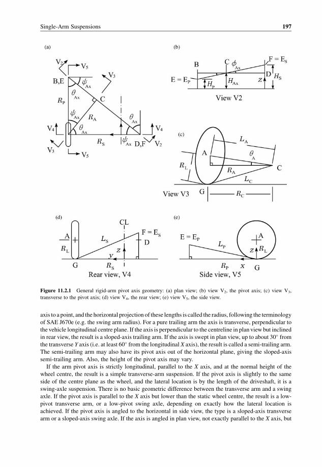
Figure 11.2.1 General rigid-arm pivot axis geometry: (a) plan view; (b) view V2, the pivot axis; (c) view V3,

transverse to the pivot axis; (d) view V4, the rear view; (e) view V5, the side view.

axis to a point, and the horizontal projection of these lengths is called the radius, following the terminology

of SAE J670e (e.g. the swing arm radius). For a pure trailing arm the axis is transverse, perpendicular to

the vehicle longitudinal centre plane. If the axis is perpendicular to the centreline in plan view but inclined

in rear view, the result is a sloped-axis trailing arm. If the axis is swept in plan view, up to about 30� fromthe transverse Y axis (i.e. at least 60� from the longitudinal X axis), the result is called a semi-trailing arm.

The semi-trailing arm may also have its pivot axis out of the horizontal plane, giving the sloped-axis

semi-trailing arm. Also, the height of the pivot axis may vary.

If the arm pivot axis is strictly longitudinal, parallel to the X axis, and at the normal height of the

wheel centre, the result is a simple transverse-arm suspension. If the pivot axis is slightly to the same

side of the centre plane as the wheel, and the lateral location is by the length of the driveshaft, it is a

swing-axle suspension. There is no basic geometric difference between the transverse arm and a swing

axle. If the pivot axis is parallel to the X axis but lower than the static wheel centre, the result is a low-

pivot transverse arm, or a low-pivot swing axle, depending on exactly how the lateral location is

achieved. If the pivot axis is angled to the horizontal in side view, the type is a sloped-axis transverse

arm or a sloped-axis swing axle. If the axis is angled in plan view, not exactly parallel to the X axis, but

Single-Arm Suspensions 197

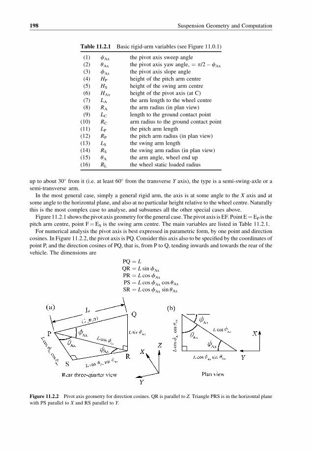
up to about 30� from it (i.e. at least 60� from the transverse Y axis), the type is a semi-swing-axle or a

semi-transverse arm.

In the most general case, simply a general rigid arm, the axis is at some angle to the X axis and at

some angle to the horizontal plane, and also at no particular height relative to the wheel centre. Naturally

this is the most complex case to analyse, and subsumes all the other special cases above.

Figure 11.2.1 shows the pivot axis geometry for the general case. The pivot axis is EF. Point E¼EP is the

pitch arm centre, point F¼ES is the swing arm centre. The main variables are listed in Table 11.2.1.

For numerical analysis the pivot axis is best expressed in parametric form, by one point and direction

cosines. In Figure 11.2.2, the pivot axis is PQ. Consider this axis also to be specified by the coordinates of

point P, and the direction cosines of PQ, that is, from P to Q, tending inwards and towards the rear of the

vehicle. The dimensions are

PQ ¼ L

QR ¼ L sin fAx

PR ¼ L cos fAx

PS ¼ L cosfAx cos uAxSR ¼ L cos fAx sin uAx

Table 11.2.1 Basic rigid-arm variables (see Figure 11.0.1)

(1) cAx the pivot axis sweep angle

(2) uAx the pivot axis yaw angle, ¼ p/2�cAx

(3) fAx the pivot axis slope angle

(4) HP height of the pitch arm centre

(5) HS height of the swing arm centre

(6) HAx height of the pivot axis (at C)

(7) LA the arm length to the wheel centre

(8) RA the arm radius (in plan view)

(9) LC length to the ground contact point

(10) RC arm radius to the ground contact point

(11) LP the pitch arm length

(12) RP the pitch arm radius (in plan view)

(13) LS the swing arm length

(14) RS the swing arm radius (in plan view)

(15) uA the arm angle, wheel end up

(16) RL the wheel static loaded radius

Figure 11.2.2 Pivot axis geometry for direction cosines. QR is parallel to Z. Triangle PRS is in the horizontal plane

with PS parallel to X and RS parallel to Y.


The direction cosines (l, m, n) in positive (X, Y, Z) directions are therefore

l ¼ � PS

PQ¼ � cos fAx cos uAx

m ¼ � SR

PQ¼ � cosfAx sin uAx

n ¼ QR

PQ¼ sin fAx

It is easily confirmed that, as is necessary,

l2 þm2 þ n2 ¼ cos2fAxðsin2 uAx þ cos2 uAxÞþ sin2fAx ¼ 1

Table 11.2.2 summarises the conversion equations between the axis angles and the direction cosines as

specified above.

It is really required to relate the wheel steer and camber angle changes to the suspension bump rather

than just to the wheel centre bump. The suspension bump is the vertical position of the lowest point of the

wheel, in the contact patch, the wheel considered geometrically as of constant radius, effectively the

loaded radius RL. With wheel bump, the contact point height is

ZCP ¼ ZW � RL cos g

The static (initial) value is

ZCP0 ¼ ZW0 � RL cos g0

If the ground plane is the datum level plane, then this is zero. The actual suspension bump is

zS ¼ ZCP � ZCP0 ¼ ðZW � ZW0ÞþRLðcos g0� cos gÞ

or

zS ¼ zw þRLðcos g0� cos gÞ

For a small camber angle, the wheel centre may therefore be taken as having the same vertical position

change as the suspension bump, but preferably the effect of camber variation would be included,

particularly for large camber angle changes (e.g. for a swing axle or other short transverse arm).

Table 11.2.2 Pivot axis angle and direction cosine conversion equations

l ¼ �cosfAx cos uAx

m ¼ �cosfAx sin uAx

n ¼ sin fAx

fAx ¼ asin ðnÞ

uAx ¼ atan

�m

l

�¼ p

2� cAx

cAx ¼ atan

�l

m

�¼ p

2� uAx


Considering a simple trailing arm, with the wheel also rotationally fixed relative to the arm, as the

arm rises the lowest point of the wheel is not a fixed point of the wheel. Hence, there is no very simple

direct solution for the lowest point in general. Further analysis of the wheel bottom point is given in

Section 5.8.

Consider the vertical plane transverse to the pivot axis, Figure 11.2.1(c), which is not the same as the

plane of the wheel axis. Given the initial dimensions, the radius from the pivot axis to the contact patch

point can be established, as can the angle of this line. However, this is complicated by any out-of-

horizontal inclination of the pivot axis. The required arm bump angle for any suspension bump can then be

solved explicitly. With the datum plane at ground level, in the initial position,

ZW0 ¼ RL cos g0

Numerically, onemethod is to project the pivot axis into the longitudinal vertical plane of thewheel centre,

giving the pitch centre point EP, and into the transverse vertical plane giving point ES, the swing centre

point. The perpendicular may be dropped onto the pivot axis from the wheel centre. The length of the

perpendicular follows, as does the angle.

Given the arm angular position angle uA, to calculate the wheel centre bump,

zW ¼ LAðsin uA� sin uA0ÞcosfAx

The suspension bump is

zS ¼ zW þ RLðcos g0�cos gÞ

This gives the suspension bump as

zS ¼ LAðsin uA� sin uA0ÞcosfAx þ RLðcos g0 � cos gÞ

Direct solution would require an algebraic relationship between the camber angle g and the arm angle uA,a relationship which is not known accurately in advance.

Geometrically, then, it is much more convenient to approximate the suspension bump as the wheel

centre bump, although this is not precise. This limitation is easily overcome in a numerical solution.

11.3 Wheel Axis Geometry

Wheel axis geometry was analysed in Chapter 5. The main results are summarised for convenient

reference in Table 11.3.1.

Table 11.3.1 Steer and camber angle conversion equations

l¼ cos g sin d

m¼�cos g cos d

n¼ sin g

g ¼ asin n

d ¼ atan

�� l

m

�


11.4 The Trailing Arm

The pure trailing armhas its pivot axis exactly perpendicular to thevehicle centre plane. In general, there is

wheel static camber and toe, but for simplicity initially consider these to be zero. The wheel axis is then

parallel to the pivot axis. Bump then has zero effect on steer and camber angles (Table 11.4.1). The initial

bump scrub and bump scrub variation coefficients are zero, and the geometric roll centre is at ground level.

There is a variation of the pitch arm radius, Figure 11.4.1. The arm angle is given by

sin uA ¼ ZW �HAx

LA

The initial, static, value of the arm angle is given by

sin uA0 ¼ ZW0 �HAx0

LA

and is generally non-zero. The simplest geometry occurs when the initial angle is zero, but in practice this

may give excessive braking anti-rise (Chapter 10).

Practical pure trailing arms often include some static toe and camber. These angles are always small,

and can be expected to have only a limited effect on the bump coefficients. However, this really needs to be

demonstrated rather than just claimed. Therefore it is desirable to obtain explicit expressions for them.

This is also a useful demonstration of method.

Consider a pure trailing arm with static camber angle g0. For simplicity, the pivot axis is taken as at the

same initial height as the wheel centre. For a passenger car the static camber would be 1 or 2 degrees, but

for a racing saloon with rear trailing arm it would possibly be beyond �3� (�0.05 rad). By inspection,

when the trailing arm is hypothetically rotated up to an arm angle of 90�, the camber angle has become

zero and a toe-out angle of d¼ g0 has appeared. When the arm is lowered to�90�, the camber has again

become zero, but the steer toe-out angle has become d¼�g0. Prospectively, the relationships are

d ¼ g0 sin uAg ¼ g0 cos uA

Expanding the sine and cosine series for the arm angle out to a maximum of the second-order term gives

d ¼ g0 uA

g ¼ g0ð1� 1

2u2AÞ

For small arm angles, the suspension or wheel bump is related to the arm angle simply by

uA ¼ zS

RP

Table 11.4.1 Coefficients for a pure trailing arm, no static

wheel angles, so all zero

«BS1¼ 0

«BS2¼ 0

«BC1¼ 0

«BC2¼ 0

«BScd0¼ 0

«BScd1¼ 0


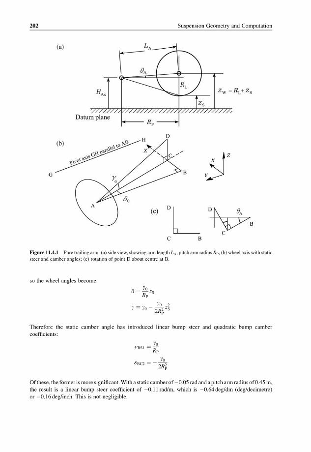
so the wheel angles become

d ¼ g0RP

zS

g ¼ g0 �g02R2

P

z2S

Therefore the static camber angle has introduced linear bump steer and quadratic bump camber

coefficients:

«BS1 ¼ g0RP

«BC2 ¼ � g02R2

P

Of these, the former ismore significant.With a static camber of�0.05 rad and a pitch arm radius of 0.45m,

the result is a linear bump steer coefficient of �0.11 rad/m, which is �0.64 deg/dm (deg/decimetre)

or �0.16 deg/inch. This is not negligible.

Figure 11.4.1 Pure trailing arm: (a) side view, showing arm length LA, pitch arm radius RP; (b) wheel axis with static

steer and camber angles; (c) rotation of point D about centre at B.


Consider now zero static camber, but a static toe-out angle of d0. At an arm angle of plus 90�, thisproduces zero steer angle and a camber angle of g ¼ �d0. At an arm angle of�90� again the steer anglehas gone to zero, but the camber angle becomes g ¼ þ d0. Prospectively, then,

d ¼ d0 cos uA

g ¼ � d0 sin uA

For small angles, as before, this becomes

d ¼ d0 � d0

2R2P

z2S

g ¼ � d0RP

zS

The result is therefore quadratic bump steer and linear bump camber coefficients

«BS2 ¼ � d0

2R2P

«BC1 ¼ � d0RP

Because the static toe angles are likely to be small in all cases, and such angles are often introduced with

the intention that the toe anglewill go even closer to zerowhen actually running, these effects are likely to

be small. For example, with d0¼�0.02 rad and RP¼ 0.45m we have «BS2¼ 0.05 rad/m2¼ 0.028 deg/

dm2.

By these simple expressions, summarised in Table 11.4.2, the effect of static wheel toe and camber

angles are easily evaluated rather than just assumed to be insignificant.

A more thorough analysis of the above geometry, now to be given, confirms that the expressions given

are good approximations, and demonstrates a useful principle. Figure 11.4.1(b) shows the wheel axis

geometry with the actual pivot axis GH.

Nowas far as changes of steer and camber angles are concerned, rotations about alternative parallel axes

are entirely equivalent, adding only a pure translation. Rotation about the real axis is of course necessary

for evaluation of actual movement, such as bump displacements. In the case of the pure trailing arm, the

real pivot axis is parallel to the Y axis, and parallel to the line AB. Therefore, for investigation of steer and

Table 11.4.2 Coefficients for a pure trailing arm,with static

wheel angles (d0, g0)

«BS1 ¼ g0RP

«BS2 ¼ � d0

2R2P

«BC1 ¼ � d0RP

«BC2 ¼ � g02R2

P

The bump scrub coefficients remain zero.


camber angles only, simply consider the wheel and wheel axis to rotate about the line AB. Positive arm

angle uA is a positive bump position, with a lowering of point C relative to B, and a lowering and forward

movement of point D, the second point of the wheel axis AD. It is changes of the position of the line AD

that are of interest, with point D rotating about B as seen in Figure 11.4.1(c). As established earlier,

AD ¼ L

BC ¼ L cos g0 sin d0CD ¼ L sin g0

After rotation, the value of XD, measured from the line AB, is

XD ¼ ðL cos g0 sin d0Þ cos uA þðL sin g0Þ sin uAThe consequent steer angle is then given by

sin d ¼ XD

L¼ cos g0 sin d0 cos uA þ sin g0 sin uA

Now introducing a small-angle approximation for the steer and camber (including cos g0¼ 1), and

expanding the arm angle to the second term of its series,

d ¼ d0ð1� 1

2u2AÞ þ g0 uA

Inserting the small-angle approximation

uA ¼ zS

RP

gives the toe-out steer angle as

d ¼ d0 þ g0RP

zS � d0

2R2P

z2S

which is in agreement with the bump steer coefficients obtained earlier (Table 11.4.2).

Similarly, for camber after rotation (see again Figure 11.4.2 (b)), relative to the line AB, the height of

point D is

ZD ¼ �ðL cos g0 sin d0Þ sin uA þðL sin g0Þ cos uAand the sine of the camber angle is given correctly by

sin g ¼ ZD

L¼ � cos g0 sin d0 sin uA þ sin g0 cos uA

Using the small-angle approximations ford and g, and expanding the armangle to the quadratic term, gives

g ¼ � d0 uA þ g0ð1� 1

2u2AÞ

Now substituting the linear approximation for the arm angle in terms of the bump position gives

g ¼ g0 �d0RP

zS � g02R2

P

z2S

again in agreement with the semi-intuitive expressions of Table 11.4.2.


This also illustrates the use of rotation about the most convenient parallel axis for investigating steer

and camber angles.

The accurate equations for the angles are collected in Table 11.4.3. These are easy enough to use, but

even for this extremely simple case are less revealing than the simpler approximate expressions of

Table 11.4.2.

11.5 The Sloped-Axis Trailing Arm

The pure trailing arm has a geometric roll centre at ground level, which may be regarded as too low. One

way to raise it is to incline (i.e. ‘slope’) the pivot axis in rear view, out of the horizontal plane,

Figure 11.5.1, introducing the appropriate bump scrub coefficient. Also, a sloped axis introduces a bump

Table 11.4.3 Pure trailing arm static toe and camber angle bump steer effects

sin d ¼ cos g0 sin d0 cos uA þ sin g0 sin uAsin g ¼ � cos g0 sin d0 sin uA þ sin g0 cos uA

Figure 11.5.1 Trailing arm with a sloping pivot axis, no static steer or camber: (a) rear three-quarter view; (b) plan

view; (c) rear view.


steer effect, whichmay be desired. For simplicity, here, thewheel is considered to have zero static toe and

camber angles. The pivot axis remains perpendicular to the vehicle centreline as seen in plan view, but is

sloped at the angle fAx in rear view, with a positive angle considered to be with the pivot axis rising as it

moves from the wheel towards the vehicle centreline.

To investigate the changes ofwheel axis angle, consider rotation of this axis about the line AJ parallel to

the real pivot axis GH. The wheel centre A does not move. The second wheel axis point B moves around

the axis AJ, in a circle around the point J. To obtain convenient approximate equations, the slope of the

pivot axis is considered to be small. This is not too bad an approximation as practical values are likely to be

less than 10�. Positive rotation of the arm, positivewheel bump,moves point B initially backwards relative

to point J, away from point I.

The basic line lengths are:

AB ¼ L

BJ ¼ L sin fAx

Relative to the line AB, with X forwards and Z upwards, approximately,

XB ¼ �L sin fAx sin uA

ZB ¼ L sin fAxð1� cos uAÞ

The resulting bump steer and camber angles are given by

sin d ¼ XB

L¼ �sin fAx sin uA

sin g ¼ ZB

L¼ sin fAxð1� cos uAÞ

With the usual small-angle approximations, as in previous sections, the resulting angles may be

expressed as

d ¼ �fAx

RP

zS

g ¼ fAx

2R2P

z2S

Table 11.5.1 Coefficients for a sloped-axis trailing arm,

with static wheel angles

«BS1 ¼ �fAx�g0RP

«BS2 ¼ � d0

2R2P

«BC1 ¼ � d0RP

«BC2 ¼ fAx�g02R2

P

«BScd0;Y ¼ tan fAx

«BScd1;Y ¼ 0


so the result is a linear bump steer coefficient and a quadratic bump camber coefficient:

«BS1 ¼ �fAx

RP

«BC2 ¼ þ fAx

2R2P

This is a similar result to the analysis for wheel static camber on the trailing arm, as in Table 11.4.2, but

with inverted signs. This is as would be expected, as the angle changes are basically a property of the

lack of parallelism of the wheel axis and the pivot axis. Therefore the sloped-axis trailing arm, for a

reasonably small inclination angle, has the properties of Table 11.5.1. The bump scrub coefficients

included in the table follow easily by inspection of the rear view.

11.6 The Semi-Trailing Arm

The semi-trailing arm has its pivot axis swept in planview, at the sweep anglecAx, considered positivewhen

thepivot axis isangled rearwardswhilstpassing towards thecentreline,asGHinFigure11.6.1.For simplicity,

in the initial analysis, the pivot axis is considered to be in the horizontal plane, that is, at zero slope angle at

wheel centre height. Also, the wheel initial toe and camber angles are taken as zero.

Figure 11.6.1 The basic semi-trailing arm,with pivot axis sweep anglecAx: (a) rear three-quarter view; (b) planview;

(c) rear view.


As the suspension arm rotates, for angle analysis the wheel axis AB may be considered to rotate about

the axis AJ parallel to the real pivot axis GH, with B rotating about J. The basic dimensions are

AB ¼ L

BJ ¼ L sin cAx

Relative to the line AJ, point B moves in a circle, with coordinates, relative to AJ, of

XB ¼ � L sin cAxð1� cos uAÞZB ¼ � L sin cAx sin uA

The bump steer and camber angles are given by

sin d ¼ XB

L¼ �sin cAxð1� cos uAÞ

sin g ¼ ZB

L¼ �sin cAxsin uA

Using the usual small-angle approximations, as in previous sections, the angles may be expressed

approximately as

d ¼ � cAx1

2u2A

g ¼ � cAx uA

and in terms of the suspension bump as

d ¼ � cAx

2R2P

z2S

g ¼ �cAx

RP

zS

so the effects introduced by the axis sweep angle are a quadratic bump steer coefficient and a linear bump

camber coefficient:

«BS2 ¼ � cAx

2R2P

«BC1 ¼ �cAx

RP

The small-angle approximations on the pivot axis anglemay not be so good in this case, as sweep angles up

to 30� may be used, but the results of this simple analysis give an excellent insight into the effects of pivot

axis sweep – specifically, a second-order bump steer and a first-order bump camber.

As discussed in Chapter 8, the lateral bump scrub for this suspension can be found simply by projecting

the real pivot axis into the transverse vertical plane of thewheel centres, giving the swing centre point ES at

height HS. The bottom point of the wheel rotates about this point, in rear view, so the lateral bump scrub

rate coefficient is

«BScd0;Y ¼ HS

RS

¼ HS

RP

tan cAx


where LP¼ LS tan cAx is the pitch arm length, Figure 11.0.1. Therefore, approximately,

«BScd0;Y ¼ HS

RP

cAx

and the lateral bump scrub rate variation coefficient is

«BSc1d;Y ¼ 1

RS

¼ cAx

RP

These results are summarised in Table 11.6.1, including superposed terms for wheel static toe and camber.

11.7 The Low-Pivot Semi-Trailing Arm

A pivot height different from the wheel centre height would normally be introduced to change the

longitudinal properties, such as the anti-lift or anti-rise.

From the principle of the parallel axis rotation, it is evident that a lowering of the pivot axis should have

no effect on the bump steer or bump camber angles.

However, this may be a confusing point, because when the pivot axis is at a different height from the

wheel centre, then the second-order bump steer («BS2) of the semi-trailing arm seems to become

asymmetrical about the static bump position. In effect this would introduce a first-order bump steer

«BS1 ¼ ðRL�HAxÞ«BS2

This is typically a small effect, but not really negligible; for example, LP¼ 0.450m, RL¼ 0.300m,

HAx¼ 0.150m, cAx¼ 0.30 rad, «BS2¼�0.741 rad/m2, «BS1¼�0.111 rad/m¼�0.64 deg/dm. However,

the use of this term presupposes that thewheel static steer and camber angles are specifiedwhen thewheel

centre is at the same height as the pivot axis. If these are specified at the static position, as they would

normally be, then the effects are automatically accounted for, and compensated, with no resulting first-

order effect other than that from thewheel axis angles.When thewheel angles are specified at the level arm

position, at the static position there are extra wheel axis angles that offset the above effect.

Table 11.6.1 Coefficients for a semi-trailing arm with

sloped axis and static wheel angles

«BS1 ¼ �fAx � g0RP

«BS2 ¼ �cAx þ d0

2R2P

«BC1 ¼ �cAx þ d0RP

«BC2 ¼ fAx � g02R2

P

«BScd0;Y ¼ HS

RS

¼ HS tan cAx

RP

«BScd1;Y ¼ � 1

RS

¼ � tan cAx

RP


The bump scrub may be affected considerably, of course, but the equations of Table 11.6.1 continue to

apply.

Varying the axis height at constant arm radius will vary the static arm length, which would change the

relationship between the arm angle and suspension bump, so having some small, but non-zero, effect on

the coefficients. Numerical results do show some small effects due to axis height.

11.8 The Transverse Arm

The basic transverse arm, equivalent to the simple swing axle, has a pivot axis parallel to the vehicle

centreline, at or close to the wheel centre height. For a true swing axle, the swing arm length is somewhat

less than half of the track, wheel lateral location being by the driveshafts which are pivoted at the sides of

the final drive unit, Figure 11.8.1. An extra arm is used to control the longitudinal position of the wheel,

hence also completing definition of the pivot axis. The pitch arm length and radius are infinite, and

therefore unsuitable for use in some equations.

In the absence of wheel static steer and camber, it is evident that the wheel camber angle is

g ¼ � uA

and the steer angle remains zero. Therefore, for this simple case, nominally,

«BC1 ¼ � 1

RS

The lateral bump scrub rate is

«BScd0;Y ¼ HAx

RS

and the lateral bump scrub rate variation is

«BScd1;Y ¼ � 1

RS

The introduction of static steer and camber angles has some interesting effects at large arm angles,

approaching 90�, beyond the practical range but of interest for geometry and for accurate analytic

expressions, because at an arm angle of 90� the properties are discontinuous.

Figure 11.8.1 The simple transverse arm (swing axle), rear view.


Introducing a static camber angle g0, within the practical range of operation this simply adds g0 to thebump camber. Introducing a positive static toe-out angle d0, at an arm angle of 90� (p/2 rad) the

camber angle becomes (p/2� d0) and the steer angle is zero. If d0 is negative (i.e. a toe-in), then the camber

at 90� arm angle becomes�(p/2� d0). At – p/2 arm angle, the camber angle becomes –(p/2� d0) and thesteer angle is zero. In fact in these extreme arm positions the result depends on an infinitesimal toe-in or

toe-out.

Figure 11.8.2 shows the plan view of a swing axle with static toe angle. The wheel axis is AB, and line

AC is the perpendicular to the pivot axis.When the armmoves in bump, thewheel centre Amoves around

C, and so towards C in the plan view. Therefore the steer angle is given by

tan d ¼ LA tan d0LA cos uA

¼ tan d0cos uA

As the arm angle approaches 90�, the tangent of the steer angle goes to infinity, and the steer angle tends tosign(d0) times p/2 (90�). Considering practical cases, for a small arm angle the approximation may be

made that

tan d � tan d0

ð1� 12u2AÞ

� tan d0ð1þ 1

2u2AÞ

This then gives

d � d0 þ d0

2R2A

z2S

so introducing a quadratic bump steer coefficient

«BS2 ¼ d0

2R2A

Because the static steer angle is likely to be small, the value of this is not a very significant effect in

practice. Within the practical range,

d � d0

g ¼ g0�1

RS

zS

Table 11.8.1 summarises the results.

Figure 11.8.2 The swing axle with static toe angle, plan view.


11.9 The Sloped-Axis Transverse Arm

The transverse-arm pivot axis may be sloped out of the horizontal plane, at angle fAx whilst remaining

parallel to the centreline in plan view, giving the sloped-axis transverse arm. Typically this is done to

obtain anti-squat and anti-rise characteristics, or bump steer, to be analysed here. For consistency with

trailing and semi-trailing arms, positive slope angle fAx will be considered to be when the axis rises

towards the rear of the vehicle. Practical swing axle design may use positive or negative values of pivot

axis inclination.

Figure 11.9.1 illustrates this case. For practical values of axis inclination, the effect on camber is small,

but the effect on steer is significant. In Figure 11.9.1(a), when thewheel bump is zW� zS, the centre of the

wheel will move forwards by zS tan fAx with a resulting bump toe angle (toe-out as positive) of

d ¼ � zS tan fAx

RS

with, therefore, a first bump steer coefficient

«BS1 ¼ � tan fAx

RS

� �fAx

RS

Table 11.9.1 summarises the results for this type of rigid-arm suspension.

Table 11.8.1 Coefficients for a simple transverse arm, with

static wheel angles

«BS1 ¼ 0

«BS2 ¼ d0

2R2A

� 0

«BC1 ¼ � 1

RS

«BC2 ¼ 0

«BSc0d;Y ¼ HAx

RS

«BScd1;Y ¼ � 1

RS

Figure 11.9.1 The transverse arm with sloped axis: (a) side view, (b) plan view.


Table 11.9.1 Coefficients for a sloped-axis transverse arm,

with static wheel angles

«BS1 ¼ �fAx

RS

«BS2 ¼ 0

«BC1 ¼ � 1

RS

«BC2 ¼ 0

«BScd0;Y ¼ HAx

RS

«BScd1;Y ¼ � 1

RS

As a matter of interest, in 1940 Henry Ford was granted a patent for a swing axle explicitly featuring

a slope angle to give bump toe-out, Figure 11.9.2. With a large load on the vehicle, or in riding bumps,

the large first bump camber coefficient of the swing axle causes rather a large camber angle with

associated side forces, which cause excessive tyre wear. This can be offset by introducing bump toe-

out (negative «BS1) to reduce the net side force to zero. The relevant tyre characteristics are the

cornering stiffnessCa relating the cornering force to the slip angle, and the camber stiffnessCg relating

the side force to the camber angle. For a suspension bump zS, the first-order bump steer and camber

angles are

d ¼ «BS1zS

g ¼ «BC1zS

The consequent tyre side force is

FY ¼ Cad þ Cgg

¼ Ca«BS1zS þ Cg«BC1zS

To eliminate the bump side force requires

«BS1«BC1

¼ � Cg

Ca

Now the ratio of the tyre coefficients is mainly a characteristic of the tyre carcase construction. In the

days of the Ford patent, bias-ply tyres were the norm, with a ratio of about 0.15. Nowadays, radial-ply

tyres are normal for passenger cars, with a ratio of about 0.05. A swing axle has a first bump camber

coefficient of about�1.7 rad/m (�10 deg/dm), so for bias-ply tyres the required bump steer coefficient

is about plus 1.5 deg/dm, and for radial ply tyres about 0.5 deg/dm. Using, from Table 11.9.1,

fAx ¼ �«BS1RS

with a swing arm radius of about 0.6m, the required axis slope is�9� for bias ply tyres and�3� for radialply tyres. The negative slope means that the axis should be down towards the rear, in agreement with

Figure 11.9.2.


11.10 The Semi-Transverse Arm

Analogous to the semi-trailing arm, the semi-transverse arm has a pivot axis in the horizontal plane, but

angled in planview, the pivot axis being fairly closely but not exactly parallel to theX axis. For consistency

with semi-trailing arms, the angle of the axis can be measured alternatively from the negative Y-axis

Figure 11.9.2 A swing axle with bump toe-out to compensate for side forces resulting from bump camber action

(Ford, 1937).


direction (left wheel), giving the sweep angle cAx. However, as in Figures 11.0.1 and 11.10.1, the actual

deviation from a simple transverse arm is the complementary angle, the axis yaw angle, which will be

denoted by uAx:

uAx ¼ p2� cAx

This angling of the axis has several effects. In Figure 11.10.1, dropping a perpendicular from the wheel

centre to the pivot axis, it may be seen that thewheel centre Amoves in an arc about point C, the foot of the

perpendicular.

The radius of the arc of point A is the arm length LA. As the wheel bumps or droops, the wheel centre A

moves, in plan view, towards C, by a distance p given by

p ¼ LAð1� cos uAÞ ¼ LA1

2

zS

RA

� �2

� 1

2RA

z2S

The movement of the wheel centre in the longitudinal X direction is

XA ¼ p sin uAx � uAx2RA

z2S

There is therefore a bump steer angle, approximately

d ¼ � XA

LAB¼ �XA

RA

¼ � uAx

2R2A

z2S

consequently giving a second bump steer coefficient

«BS2 ¼ � uAx

2R2A

The pitch and roll force characteristics are solved in the usual way, projecting the axis into the relevant

planes to obtain the swing centre ES and pitch centre EP points. Table 11.10.1 summarises the coefficients

for the semi-transverse arm.

Figure 11.10.1 Semi-transverse arm in planview, axis sweep anglecAx from theY axis, axis yawangle uAx from theX

axis.


11.11 The Low-Pivot Semi-Transverse Arm

A low pivot axis on a transverse arm is typically used to reduce the height of the roll centre (e.g. the low-

pivot swing axle). The effect on bump steer is similar to the effect on the semi-trailing arm. The existing

second-order bump steer, if any, is no longer symmetrical about the static position, so some first-order

bump steer is introduced:

«BS1 ¼ ðRL�HAxÞ«BS2

However, this again assumes that the wheel static steer and camber are specified at the horizontal arm

position. Normally they would be specified at the static position. At the horizontal arm position, these

angles are different, introducing additional effects, and compensating for the above term.

The bump scrub coefficients continue as in Table 11.10.1 with appropriate evaluation of the swing

centre height HS.

11.12 General Case Numerical Solution

The computer numerical solution of the rigid arm is quite easily performed, given certain standard three-

dimensional coordinate geometry routines discussed in a subsequent chapter. The basic problem is

specified by the static position in vehicle coordinates, Figure 11.12.1, by

(1) the coordinates of a point A on the pivot axis (xA, yA, zA),

(2) the direction cosines of the pivot axis (lA, mA, nA),

(3) the coordinates of a point W on the wheel axis (xW, yW, zW),

(4) the direction cosines of the wheel axis (lW, mW, nW).

Other information required includes the track, and thewheel centre position, if this is not already known to

be point W.

Two distinct analyses are required, static (the initial position) and displacement (arm rotated, leading to

bump coefficients).

Table 11.10.1 Coefficients for a semi-transverse arm,

including axis slope and static wheel angles

«BS1 ¼ �fAx

RA

«BS2 ¼ �ð uAx� d0Þ2R2

A

«BC1 ¼ � 1

RS

«BC2 ¼ 0

«BScd0;Y ¼ HS

RS

«BScd1;Y ¼ � 1

RS


In a static analysis of the suspension it is desired to obtain:

(1) the pitch centre, pitch arm radius and length;

(2) the swing centre, swing arm radius and length;

(3) the bump scrub rate coefficient;

(4) the roll centre height.

The pitch centre is obtained by intersecting the pivot axis with the vertical longitudinal plane of the

wheel–ground contact point, effectively of the wheel centre. The swing centre is obtained by intersecting

the pivot axis with the vertical transverse plane of the two wheel centres of the axle. The intersection of a

linewith a plane requires standard routines discussed in Chapter 15. In special cases, one or other of these

points may be at infinity (e.g. a pure trailing arm or a pure transverse arm).

The bump scrub rate coefficient «BScd0 follows as HS/RS in the general case, and the geometric roll

centre height as 12T«BScd0.

In the displacement analysis, for a rotation of the arm, about the pivot axis, by some specified angle, it is

required to determine

(1) the wheel steer angle,

(2) the wheel camber angle,

(3) the suspension bump,

(4) the local scrub rate,

with a series of such results through the suspension range, a quadratic polynomial curve fit then giving the

bump coefficients. Interchange of the wheel axis angle specification (d, g) and the wheel axis direction

cosines (lW, mW, nW) is required, as given in Table 11.3.1.

The underlying geometrical problem is to rotate one line, the wheel axis, about another line, the pivot

axis. The easiest way to do this is to use two points on thewheel axis, and rotate each point about the pivot

axis, the newpoint positions then defining the newwheel axis. Thefirst point on the axis can be the pointW

as originally specified – typically but not essentially the wheel centre. The second point can be any

reasonable well-separated point, P, say at separation L from pointW. Then the initial position of point P is

xP ¼ xW þ LlW

yP ¼ yW þ LmW

zP ¼ zW þ LnW

Figure 11.12.1 Pivot axis throughA andwheel axis throughW, each axis defined by a point and direction cosines. P is

a methodological second point on the wheel axis.


At the scale of vehicle suspensions, it is convenient to use a separation of 1 metre. The direction cosines

of the new axis then follow easily, and thence the wheel steer and camber angles for that bump position.

The residual problem, then, is the rotation of one point about a line by a specified angle. This is easy in

two dimensions, so one approach is to specify a local coordinate system with the circular motion of the

point in a local coordinate plane with perpendicular unit vectors (v; w) in the plane perpendicular to the

axis u, Figure 11.12.2. The axis unit vector is already known. Drop a perpendicular from the point P onto

the axis, with foot F. The length PF is the arc radius R for that point. One in-plane unit vector can be

determined as being along FPand of unit length. The third unit vector, also in the plane of rotation, can then

be determined by a vector cross product of the two known unit vectors,

w ¼ ðlw;mw; nwÞ ¼ u� v ¼i j k

lu mu nu

lv mv nv

��

��

where the determinant is to be expanded with the usual sign alternations.

For a right-hand rotation by angle u about the axis direction, the coordinates of the new position of P are

then given by

xP ¼ xF þ lv cos uþ lw sin u

yP ¼ yF þ mv cos uþ mw sin u

zP ¼ zF þ nv cos uþ nw sin u

with P rotating in the ðv; wÞ plane as desired. Hence a new point P is determined.

By doing this for any two distinct points on thewheel axis, the newwheel axis is found, and the steer and

camber angles follow.

In practice, the above is quite easily programmed, given the necessary three-dimensional routines, and

is accurate.

11.13 Comparison of Solutions

Table 11.13.1 shows how the accurate numerical solution compares with the approximate algebraic

expressions from the earlier Tables 11.6.1 (semi-trailing arm) and 11.10.1 (semi-transverse arm). The

approximate expressions are evidently good enough formental imagery of the effects, and even for general

design use.

Figure 11.12.2 Generation of local coordinate system for rotation of a point about an axis by a specified angle.


Table 11.13.1 Suspension: rigid-armanalysis, byRigidArm.f90 program

Arm type = Pure trailing arm, zero steer and camber

Pivot theta (deg) = 90.000

Pivot psi (deg) = 0.000

Pivot phi (deg) = 0.000

Wheel steer (deg) = 0.000

Wheel camber (deg) = 0.000

Pitch arm length (m) = 0.450

numerical analytic

epsBS1 (deg/dm) = 0.000 0.000

epsBS2 (deg/dm2) = 0.000 0.000

epsBC1 (deg/dm) = 0.000 0.000

epsBC2 (deg/dm2) = 0.000 0.000

Arm type = Trailing arm with sloped axis







numerical analytic

epsBS1 (deg/dm) = -1.114 -1.111

epsBS2 (deg/dm2) = 0.000 0.000

epsBC1 (deg/dm) = 0.000 0.000

epsBC2 (deg/dm2) = 0.125 0.123

Arm type = Pure trailing arm, with steer and camber







numerical analytic

epsBS1 (deg/dm) = 0.444 0.444

epsBS2 (deg/dm2) = -0.050 -0.049

epsBC1 (deg/dm) = -0.444 -0.444

epsBC2 (deg/dm2) = -0.050 -0.049

Arm type = Semi-trailing arm, zero steer and camber







(continued )


Table 11.13.1 (Continued )

numerical analytic

epsBS1 (deg/dm) = 0.000 0.000

epsBS2 (deg/dm2) = -0.465 -0.444

epsBC1 (deg/dm) = -4.139 -4.000

epsBC2 (deg/dm2) = 0.000 0.000

Arm type = Semi-trailing arm, with sloped axis







numerical analytic

epsBS1 (deg/dm) = -1.171 -1.111

epsBS2 (deg/dm2) = -0.461 -0.444

epsBC1 (deg/dm) = -4.139 -4.000

epsBC2 (deg/dm2) = 0.146 0.123

Arm type = Semi-trailing arm, with steer and camber







numerical analytic

epsBS1 (deg/dm) = 0.441 0.444

epsBS2 (deg/dm2) = -0.510 -0.494

epsBC1 (deg/dm) = -4.581 -4.444

epsBC2 (deg/dm2) = -0.049 -0.049

Arm type = Pure transverse arm, zero steer and camber






Arm radius (m) = 0.600

numerical analytic

epsBS1 (deg/dm) = 0.000 0.000

epsBS2 (deg/dm2) = 0.000 0.000

epsBC1 (deg/dm) = -9.596 -9.549

epsBC2 (deg/dm2) = 0.000 0.000



Arm type = Transverse arm, with sloped axis







numerical analytic

epsBS1 (deg/dm) = -0.848 -0.833

epsBS2 (deg/dm2) = 0.000 0.000

epsBC1 (deg/dm) = -9.596 -9.549

epsBC2 (deg/dm2) = 0.000 0.000

Arm type = Pure transverse arm, with steer and camber







numerical analytic

epsBS1 (deg/dm) = -0.012 0.000

epsBS2 (deg/dm2) = 0.029 0.000

epsBC1 (deg/dm) = -9.590 -9.549

epsBC2 (deg/dm2) = 0.000 0.000

Arm type = Semi-transverse arm, zero steer and camber







numerical analytic

epsBS1 (deg/dm) = 0.000 0.000

epsBS2 (deg/dm2) = -0.220 -0.208

epsBC1 (deg/dm) = -9.593 -9.549

epsBC2 (deg/dm2) = 0.000 0.000

Arm type = Semi-transverse arm, with sloped axis







(continued )



numerical analytic

epsBS1 (deg/dm) = -0.878 -0.833

epsBS2 (deg/dm2) = -0.221 -0.208

epsBC1 (deg/dm) = -9.593 -9.549

epsBC2 (deg/dm2) = 0.000 0.000

Arm type = Semi-transverse arm, with steer and camber







numerical analytic

epsBS1 (deg/dm) = 0.080 0.000

epsBS2 (deg/dm2) = -0.193 -0.208

epsBC1 (deg/dm) = -9.678 -9.549

epsBC2 (deg/dm2) = -0.002 0.000

11.14 The Steered Single Arm

The single-arm suspension has sometimes been used at the front with steering. Two examples are the

Dubonnet type, Figure 1.5.2 and the long transverse arm, Figure 1.6.3. The bump steer depends on the

steering linkage, as described in Chapter 6, but in both cases accurate steering is possible. However, the

steer axis (kingpin) inclination angle and steer axis (kingpin) caster angle, which affect steering feel, are of

importance. The dependence of these on suspension bump can be represented by quadratic expressions in

the usual way:

uKI ¼ uKI0 þ «BKI1zS þ «BKI2z2S

uKC ¼ uKC0 þ «BKC1zS þ «BKC2z2S

The kingpin inclination angle is generally taken as positive when it slopes inwards at the top, that is,

analogous to thewheel camber angle but of reversed sign. The caster angle is positivewhen the axis slopes

to the rear as it rises. The kingpin axis is fixed relative to the single arm, so the bump kingpin inclination

coefficients are essentially the same as the bump camber coefficients.

The kingpin axis is approximately vertical, Figure 11.14.1, specified typically by two points, the ball

joints, easily giving the parametric form of the steer axis line. Numerical solution of the moved axis then

follows by the same principles as for the wheel axis. It is apparent that in the case of the transverse arm

there will be large changes of inclination angle, which is undesirable, with small changes of caster angle.

In contrast, the trailing and semi-trailing arms have small changes of kingpin inclination angle but large

changes of caster angle:

«BKI1 ¼ cos uAxRA

«BKC1 ¼ � sin uAxRA

¼ � cos cAx

RA

This large caster angle variation of the steered trailing arm, over 10� in each direction, is a serious

difficulty, and contributed to the early demise of the type in favour of the double-wishbone suspension.

The trailing arm has severe brake divewith the caster change because the arm adds to the body pitch angle

effect. The leading arm, with extreme anti-dive, is less of a problem in this respect.


Figure 11.14.1 The single-arm suspension with a kingpin axis for steering.

The steered transverse arm was more successful, and was used for many years on small rear-engined

family saloons. To minimise the kingpin inclination variation and the camber change, the arm was made

long, with the pivot axis close to the vehicle centreline, Figure 1.6.3.

11.15 Bump Scrub

In the case of a rigid arm with zero slope of the pivot axis, and no wheel angles, the bump scrub is

particularly simple to analyse. In Figure 11.15.1(a), which is the view along the pivot axis, the distance

from that axis to the central contact point is LC (not LA to the wheel centre), and the angle of this radius

from the horizontal is uC. The radiusRC is slightly different fromRA because of thewheel camber, but this

small difference is neglected here.

In the plan view of Figure 11.15.1(b), for a locked-wheel vehicle, the resulting total scrub will be

perpendicular to the pivot axis, along direction AC. For a (small) suspension bump zS, the total scrub is

s ¼ LC du sin uC ¼ zS tan uC

The total locked-wheel scrub rate coefficient is therefore

«BScd0;T ¼ tan uC ¼ HAx

RC

� HAx

RA

This total locked scrub resolves into directions along the prospectively rolling wheel and perpendicular to

it. Normally the small wheel steer angle is neglected, so that the scrub can be resolved more simply into

vehicle X (longitudinal) and Y (lateral) components. The longitudinal scrub coefficient, relevant to

braking, is

«BScd0;X ¼ � «BScd0;T sin uAx ¼ � HAx sin uAxRA

but

RP sin uAx ¼ RA

so

«BScd0;X ¼ �HAx

RP


Similarly, the Y component of the scrub gives a lateral scrub rate coefficient

«BScd0;Y ¼ «BSc0;T cos uAx

giving

«BScd0;Y ¼ HAx

RS

This lateral component is the one relevant to handling and the roll centre height, and the result here agrees

with the simple calculation normally used.

The case of a pivot axis with slope ismore complex, Figure 11.15.2.With an arm angularmotion du, thetangential displacement of the contact point of the locked wheel is

t ¼ LC du

which occurs in the sloping plane perpendicular to the axis. This resolves into

s1 ¼ t sin uC

in the horizontal plane and

s2 ¼ t cos uC

in the sloping plane. This latter part further resolves into

s3 ¼ t cos uC sin fAx

Figure 11.15.1 Bump scrub of the rigid arm without pivot axis slope.


Figure 11.15.2 Bump scrub geometry for a rigid arm with pivot axis slope.

in the horizontal plane and

zS ¼ t cos uC cosfAx

vertically. The Y component of the scrub is

sY ¼ s1 cos uAx þ s3 sin uAx

¼ t sin uC cos uAx þ t cos uC sin fAx sin uAx

The lateral scrub rate is therefore

«BScd0;Y ¼ sY

zS¼ tan uC cos uAx

cosfAx

þ sin fAx sin uAxcos fAx

Now

HAx

RS

¼ HAx

RA

RA

RS

¼ tan uCcos fAx

cos uAx

and

sin uAx ¼ LCD

RS

so

«BScd0;Y ¼ HAx

RS

þ LCD tan fAx

RS

¼ HAx

RS

þ HS �HAx

RS

¼ HS

RS


whereHS is the height of the swing centre, so the conventional simple expression is applicable even when

the axis is sloped.

Of course, the argument for this property in the case of the force roll centre is very easily established,

because the jacking force must be such that the moment of the lateral force about the axis is zero.

References

Ford, H. (1937). Motor vehicle. US Patent 2,214,456, filed 1 Nov 1937, granted 10 Sep 1940.

————— // —————


12

Double-Arm Suspensions

12.1 Introduction

This chapter deals with suspensions having location by two arms rather than the single-rigid-arm type of

the previous chapter. The most common form of double-arm suspension is the double-transverse-arm

suspension. Another type is the double-trailing-arm type. Example diagrams of these and others are given

in Chapter 1. Strut-and-arm suspensions are also considered here, as variants of the double-arm type.

Double-transverse-arm suspensions are also known as double-lateral-arm, double-wishbone or double

A-arm. The terms ‘wishbone’ and ‘A-arm’ are effectively interchangeable, at least as far as geometric

properties are concerned – these names merely reflect the appearance of the arm, arising from the method

of construction.

The common strut and transverse-arm suspension can, for geometric analysis, be considered as

effectively a double-transverse-arm type in which the upper arm has more or less infinite length. This

places some limitations on the geometric design possibilities, as will be shown.

The earliest cars had rigid front axles which suffered from steering geometry problems, as described in

Chapter 1. To minimise this, the front springs had to be made stiff, to limit suspension movement.

Independent front suspension, with its superior steering geometry, was introduced to allow soft springs

and hence better ride quality whilst retaining good steering properties. The earliest independent types

were the Dubonnet single leading or trailing arm, and the double transverse arm. The Dubonnet type soon

fell from favour. The early double transverse-arm type had equal-length arms, parallel and level. Soon, the

arms were made unequal in length, and placed at various angles to the horizontal in front and side view.

Also, one or both arm pivot axes were sometimes angled in plan view. These changes to the details were

made to obtain certain geometric properties giving desired dynamic properties. This chapter relates the

geometric configuration to the consequent coefficients.

With double-arm suspensions, the steering properties, such as the bump steer coefficients, are

dependent on the details of the steering mechanism, as already discussed to some extent in Chapter 5.

This can be separated out from the basic properties of the arm geometry. Therefore the arm geometry is

used to control the roll centre, the bump camber properties, the anti-dive and the bump caster. Specifically,

the lateral coefficients to be controlled are:

(1) the lateral bump scrub rate «BScd0,Y giving the roll centre height;

(2) the lateral bump scrub rate variation «BScd1,Y giving the roll centre movement;

(3) the linear bump camber coefficient «BC1;(4) the quadratic bump camber coefficient «BC2.


The longitudinal coefficients to be controlled are:

(1) the longitudinal bump scrub rate «BScd0,X giving the anti-dive;

(2) the longitudinal bump scrub rate variation «BScd1,X giving anti-dive variation;

(3) the linear bump caster coefficient «Bcas1;(4) the quadratic bump caster coefficient «Bcas2.

There are therefore eight coefficients to be controlled. In the analysis process, the geometry is specified

and the coefficients are deduced. In the design process, the values of the coefficients are specified, and the

required geometry is deduced. The appropriate steering can then be added. In practice, of course, there

may be some iteration in this process.

To control the eight variables as desired, the system must have at least eight suitable degrees of

design freedom, four in the transverse properties and four in the longitudinal ones. Basically, these are the

two arm lengths and the two arm angles to the horizontal. As seen in front view, this gives the first four

factors, and in side view the second four. Strictly speaking, every coordinate affects every coefficient, but

in practice the individual coefficients can be quite closely related to particular individual geometric

features.

12.2 Configurations

Figure 12.2.1 shows a range of basic possibilities for the double-arm suspension. The pivot axis of each

arm may be at almost any angle in plan view, although always approximately horizontal. Also, the arm

lengths may vary considerably. The double transverse arm may have the pivot axes substantially parallel

with the vehicle centreline, as shown, but to obtain certain characteristics one or other arm axis may be

inclined in side view, or even more so in plan view.

The double-trailing-arm suspension seen in Figure 12.2.1(b) is simply a particular type of double arm

with the pivot axes transverse to the vehicle centreline. Figure 12.2.1(c) shows a rarer type, in which the

Figure 12.2.1 Basic layouts of double-arm suspension: (a) double transverse; (b) double trailing; (c) lower transverse,

upper leading; (d) lower leading, upper trailing; (e) lower trailing, upper leading.


lower arm is a conventional transverse arm, but the upper arm is leading and has its axis transverse. This is

geometrically, in front view, somewhat like a strut. This is a particularly extreme case of crossed axes.

In Figure 12.2.1(d,e) are seen types with one leading and one trailing arm. These are unusual, but have the

advantage that there is a Watt’s linkage effect which minimises the fore and aft movement of the wheel

centre, so these configurations are sometimes used for driven rear independent suspensions.

12.3 Arm Lengths and Angles

The three-dimensional system can be approached as two separate problems, each in two dimensions only,

one problem being the front (or rear) view controlling the transverse properties, the other being the side

view controlling the longitudinal properties. The correct analysis should really be done in a complete form

in three dimensions, but the two-dimensional approximations are useful for human understanding and for

initial design purposes.

The plane of an arm is defined as the geometric plane passing through the arm pivot axis and the centre

of the ball joint at the arm outer end.

In the vehicle end view, seeing the transverse vertical plane of the unsteered wheel centres, the plane of

the arm intersects this vertical plane to give a line of the arm. The actual pivot axis intersects the vertical

plane at the inner point of the equivalent two-dimensional arm. It is less clear exactlywhere the outer point

of the equivalent arm should be taken to be. Usually, the front-view position of the ball joint is used. This

may not agree exactlywith the plane of the arm, but is usually good enough. The result of this process is an

equivalent front view, with the arms having specific lengths and angles to the horizontal, in the static

position, Figure 12.3.1(a). The two arm lengths and two angles provide four degrees of design freedom,

and prove to be good variables in controlling the desired transverse geometrical properties. However, it

may be more convenient to think in terms of the average arm length and the length ratio or difference, and

of the average angle and the convergence angle, as will be seen. Also, the equations are more readily

expressed in terms of the ‘shortness’ of the links, the reciprocal of their length.

In side view, Figure 12.3.1(b), the plane of the arm may be intersected with the vertical longitudinal

plane of the unsteeredwheel centre along the side of thevehicle to give the line of the arm. The pivot axis of

an arm intersects this plane at the point at one end of the equivalent two-dimensional arm. Often this

particular point is at infinity. Nevertheless, its angular position to the horizontal from the wheel is

important. Again, a point must be chosen to represent the ball joint centre, and often this will be the

position of the ball joint as seen in the side view, although again this may not agree exactly with the line of

the arm found from the intersection of the planes. This discrepancy is usually small. The result of this

process is an equivalent side view,with the arms having specific lengths and angles to the horizontal, in the

static position, Figure 12.3.1(b). These two lateral-view arm lengths and two angles provide four further

degrees of design freedom, and prove to be good variables in controlling the desired longitudinal

geometrical properties. However, again, it may bemore convenient to think in terms of the average length

Figure 12.3.1 Double transverse arms, equivalent 2D mechanism: (a) front view; (b) side view.

Double-Arm Suspensions 229

and the length ratio or difference, or link shortness and shortness difference, and of the average angle and

the convergence angle (i.e. angle difference).

It will be apparent from Figure 12.3.1 that the conceptual geometrical properties are related to the

lateral-view arm lengths and angles by a similar process to theway that the lateral properties are related to

the transverse arms and angles. The lateral properties will be examined first, the longitudinal properties

then following easily.

12.4 Equal Arm Length

The earliest double-transverse-arm suspensions, seen in front view, had arms that were simply of equal

length and horizontal when in the static position, Figure 12.4.1. The basic properties are easily found by

inspection, and are shown in Table 12.4.1. The camber is unchanging. The initial bump scrub rate is zero,

implying that the roll centre is initially at ground level. The bump scrub rate variation and associated roll

centre movement depend on the lateral arm length LY.

12.5 Equally-Angled Arms

If the arms are angled in the static position, whilst remaining parallel, as in Figure 12.5.1, then the camber

is still unchangingwith bump. The arm angle is defined to be positivewhen the ball joint is higher than the

Table 12.4.1 Lateral properties of parallel horizontal double transverse arms

«BScd0;Y ¼ 0

«BScd1;Y ¼ � 1

LY

«BC1 ¼ 0

«BC2 ¼ 0

Figure 12.4.1 Parallel equal-length arms.

Figure 12.5.1 Angled parallel equal-length arms.


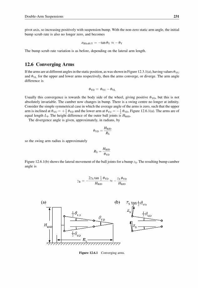
pivot axis, so increasing positively with suspension bump. With the non-zero static arm angle, the initial

bump scrub rate is also no longer zero, and becomes

«BScd0;Y ¼ �tan uY � � uY

The bump scrub rate variation is as before, depending on the lateral arm length.

12.6 Converging Arms

If the arms are at different angles in the static position, aswas shown in Figure 12.3.1(a), having values uYUand uYL for the upper and lower arms respectively, then the arms converge, or diverge. The arm angle

difference is

uYD ¼ uYU � uYL

Usually this convergence is towards the body side of the wheel, giving positive uYD, but this is not

absolutely invariable. The camber now changes in bump. There is a swing centre no longer at infinity.

Consider the simple symmetrical case in which the average angle of the arms is zero, such that the upper

arm is inclined at uYU¼ þ 12uYD and the lower arm at uYU ¼� 1

2uYD, Figure 12.6.1(a). The arms are of

equal length LY. The height difference of the outer ball joints is HBJD.

The divergence angle is given, approximately, in radians, by

uYD ¼ HBJD

RS

so the swing arm radius is approximately

RS ¼ HBJD

uYD

Figure 12.6.1(b) shows the lateral movement of the ball joints for a bump zS. The resulting bump camber

angle is

gB ¼ �2zS tan12uYD

HBJD

� � zS uYDHBJD

Figure 12.6.1 Converging arms.


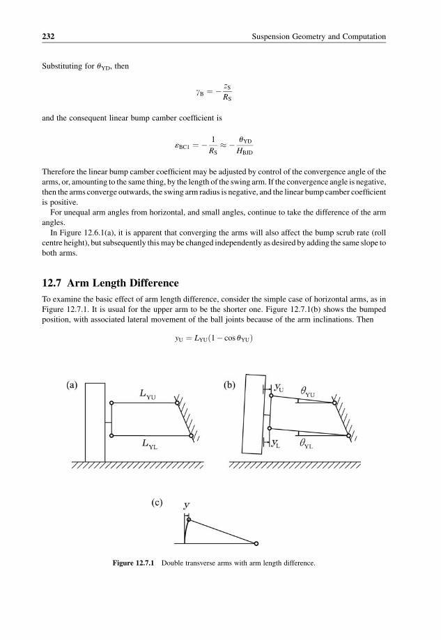
Substituting for uYD, then

gB ¼ � zS

RS

and the consequent linear bump camber coefficient is

«BC1 ¼ � 1

RS

� � uYDHBJD

Therefore the linear bump camber coefficient may be adjusted by control of the convergence angle of the

arms, or, amounting to the same thing, by the length of the swing arm. If the convergence angle is negative,

then the arms converge outwards, the swing arm radius is negative, and the linear bump camber coefficient

is positive.

For unequal arm angles from horizontal, and small angles, continue to take the difference of the arm

angles.

In Figure 12.6.1(a), it is apparent that converging the arms will also affect the bump scrub rate (roll

centre height), but subsequently thismay be changed independently as desired by adding the same slope to

both arms.

12.7 Arm Length Difference

To examine the basic effect of arm length difference, consider the simple case of horizontal arms, as in

Figure 12.7.1. It is usual for the upper arm to be the shorter one. Figure 12.7.1(b) shows the bumped

position, with associated lateral movement of the ball joints because of the arm inclinations. Then

yU ¼ LYUð1� cos uYUÞ

Figure 12.7.1 Double transverse arms with arm length difference.


Approximating the arm angle by

uYU ¼ zS

LYU

and using

cos uYU � 1� 1

2u2YU ¼ 1� z2S

2L2YU

then

yU ¼ z2S2LYU

and yL ¼ z2S2LYL

Consequently, the bump camber angle is

gB ¼ � yU � yL

HBJD

¼ � 1

2HBJD

1

LYU� 1

LYL

0@

1Az2S

In terms of the arm shortness S¼ 1/L, this is

gB ¼ � 1

2HBJD

ðSYU � SYLÞz2S

Using the arm shortness difference

SYD ¼ SYU � SYL

the bump camber angle is simply expressed as

gB ¼ � SYD

2HBJD

z2S

Hence, the arm length difference causes a quadratic bump camber coefficient

«BC2 ¼ � SYD

2HBJD

and the arm length difference may be used to control this aspect of the geometry as required. A negative

quadratic bump camber coefficient is usually desired, in which case SYD must be positive, requiring the

upper arm to be the shorter one.

12.8 General Solution

The foregoing equations are a useful guide to the effect of various geometrical changes, but with arm

convergence the bump scrub effects are not handled accurately enough for design purposes, so an

improved analysis will now be given here. However, the resulting equations are more complex, and the


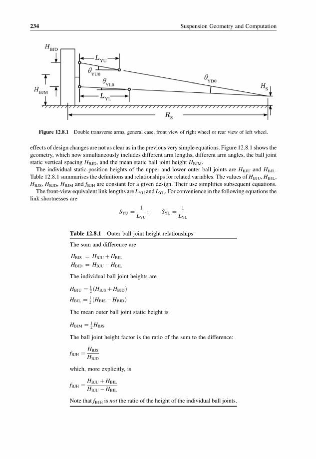
effects of design changes are not as clear as in the previous very simple equations. Figure 12.8.1 shows the

geometry, which now simultaneously includes different arm lengths, different arm angles, the ball joint

static vertical spacing HBJD, and the mean static ball joint height HBJM.

The individual static-position heights of the upper and lower outer ball joints are HBJU and HBJL.

Table 12.8.1 summarises the definitions and relationships for related variables. The values ofHBJU,HBJL,

HBJS, HBJD, HBJM and fBJH are constant for a given design. Their use simplifies subsequent equations.

The front-view equivalent link lengths are LYU and LYL. For convenience in the following equations the

link shortnesses are

SYU ¼ 1

LYU; SYL ¼ 1

LYL

Figure 12.8.1 Double transverse arms, general case, front view of right wheel or rear view of left wheel.

Table 12.8.1 Outer ball joint height relationships

The sum and difference are

HBJS ¼ HBJU þHBJL

HBJD ¼ HBJU �HBJL

The individual ball joint heights are

HBJU ¼ 12ðHBJS þHBJDÞ

HBJL ¼ 12ðHBJS �HBJDÞ

The mean outer ball joint static height is

HBJM ¼ 12HBJS

The ball joint height factor is the ratio of the sum to the difference:

fBJH ¼ HBJS

HBJD

which, more explicitly, is

fBJH ¼ HBJU þHBJL

HBJU �HBJL

Note that fBJH is not the ratio of the height of the individual ball joints.


The shortness sum and difference are

SYS ¼ SYU þ SYLSYD ¼ SYU � SYL

The initial (static position) link angles are uYU0 and uYL0, positive as shown in the figure, clockwise. These

arm angles are defined positive such that they increase in bump. Table 12.8.2 summarises useful arm angle

equations.

In Figure 12.8.1, the long triangle gives, approximately,

HBJD ¼ RS uYD

so the swing arm radius is

RS ¼ HBJD

uYD¼ HBJD

uYD0 þ SYDzS

The linear bump camber coefficient is

«BC1 ¼ � 1

RS0

¼ � uYD0HBJD

As before, the quadratic bump camber coefficient is

«BC2 ¼ � SYD

2HBJD

Table 12.8.2 Arm angle relationships

The static arm angle sum and difference are

uYS0 ¼ uYU0 þ uYL0uYD0 ¼ uYU0� uYL0

At suspension bump position zS, the link angles become

uYU ¼ uYU0 þ SYUzSuYL ¼ uYL0 þ SYLzS

The sum and difference of these angles are

uYS ¼ uYU þ uYLuYD ¼ uYU� uYL

The individual angles are

uYU ¼ 12ð uYS� uYDÞ

uYL ¼ 12ð uYS� uYDÞ

By substitution, the sum and difference are

uYS ¼ uYS0 þ SYSzSuYD ¼ uYD0 þ SYDzS


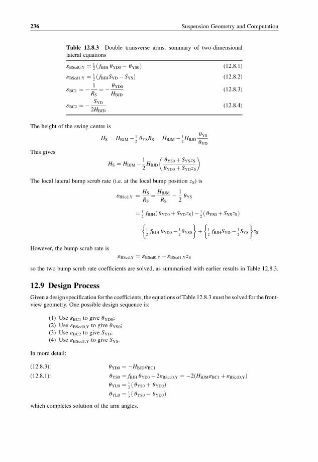
The height of the swing centre is

HS ¼ HBJM � 1

2uYSRS ¼ HBJM � 1

2HBJD

uYSuYD

This gives

HS ¼ HBJM � 1

2HBJD

uYS0 þ SYSzS

uYD0 þ SYDzS

� �

The local lateral bump scrub rate (i.e. at the local bump position zS) is

«BScd;Y ¼ HS

RS

¼ HBJM

RS

� 1

2uYS

¼ 1

2fBJHð uYD0 þ SYDzSÞ� 1

2ð uYS0 þ SYSzSÞ

¼ 1

2fBJH uYD0 � 1

2uYS0

� �þ 1

2fBJHSYD � 1

2SYS

� �zS

However, the bump scrub rate is

«BScd;Y ¼ «BScd0;Y þ «BScd1;YzS

so the two bump scrub rate coefficients are solved, as summarised with earlier results in Table 12.8.3.

12.9 Design Process

Given a design specification for the coefficients, the equations of Table 12.8.3must be solved for the front-

view geometry. One possible design sequence is:

(1) Use «BC1 to give uYD0;

(2) Use «BScd0,Y to give uYS0;(3) Use «BC2 to give SYD;

(4) Use «BScd1,Y to give SYS.

In more detail:

(12.8.3): uYD0 ¼ �HBJD«BC1

(12.8.1): uYS0 ¼ fBJH uYD0 � 2«BScd0;Y ¼ �2ðHBJM«BC1 þ «BScd0;YÞuYU0 ¼ 1

2ð uYS0 þ uYD0Þ

uYL0 ¼ 1

2ð uYS0 � uYD0Þ

which completes solution of the arm angles.

Table 12.8.3 Double transverse arms, summary of two-dimensional

lateral equations

«BScd0;Y ¼ 12ð fBJH uYD0 � uYS0Þ (12.8.1)

«BScd1;Y ¼ 12ð fBJHSYD � SYSÞ (12.8.2)

«BC1 ¼ � 1

RS

¼ � uYD0HBJD

(12.8.3)

«BC2 ¼ � SYD

2HBJD

(12.8.4)


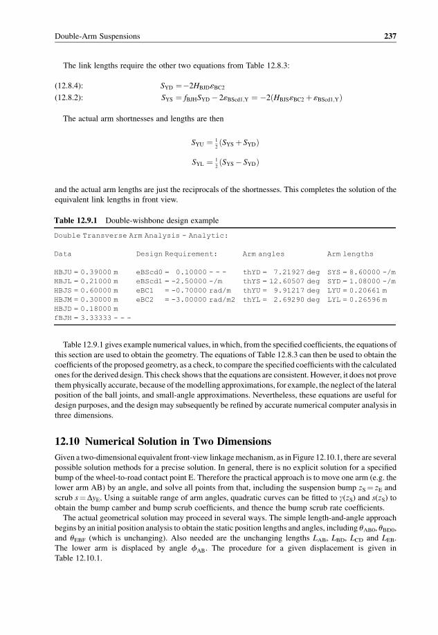
The link lengths require the other two equations from Table 12.8.3:

(12.8.4): SYD ¼�2HBJD«BC2

(12.8.2): SYS ¼ fBJHSYD � 2«BScd1;Y ¼ �2ðHBJS«BC2 þ «BScd1;YÞ

The actual arm shortnesses and lengths are then

SYU ¼ 1

2ðSYS þ SYDÞ

SYL ¼ 1

2ðSYS � SYDÞ

and the actual arm lengths are just the reciprocals of the shortnesses. This completes the solution of the

equivalent link lengths in front view.

Table 12.9.1 gives example numerical values, in which, from the specified coefficients, the equations of

this section are used to obtain the geometry. The equations of Table 12.8.3 can then be used to obtain the

coefficients of the proposed geometry, as a check, to compare the specified coefficients with the calculated

ones for the derived design. This check shows that the equations are consistent. However, it does not prove

them physically accurate, because of themodelling approximations, for example, the neglect of the lateral

position of the ball joints, and small-angle approximations. Nevertheless, these equations are useful for

design purposes, and the design may subsequently be refined by accurate numerical computer analysis in

three dimensions.

12.10 Numerical Solution in Two Dimensions

Given a two-dimensional equivalent front-view linkagemechanism, as in Figure 12.10.1, there are several

possible solution methods for a precise solution. In general, there is no explicit solution for a specified

bump of the wheel-to-road contact point E. Therefore the practical approach is to move one arm (e.g. the

lower arm AB) by an angle, and solve all points from that, including the suspension bump zS¼ zE and

scrub s¼DyE. Using a suitable range of arm angles, quadratic curves can be fitted to g(zS) and s(zS) to

obtain the bump camber and bump scrub coefficients, and thence the bump scrub rate coefficients.

The actual geometrical solution may proceed in several ways. The simple length-and-angle approach

begins by an initial position analysis to obtain the static position lengths and angles, including uAB0, uBD0,and uEBF (which is unchanging). Also needed are the unchanging lengths LAB, LBD, LCD and LEB.

The lower arm is displaced by angle fAB. The procedure for a given displacement is given in

Table 12.10.1.

Table 12.9.1 Double-wishbone design example

Double Transverse Arm Analysis - Analytic:

Data

HBJU = 0.39000 m

HBJL = 0.21000 m

HBJS = 0.60000 m

HBJM = 0.30000 m

HBJD = 0.18000 m

fBJH = 3.33333 - - -

Design Requirement:

eBScd0 = 0.10000 - - -

eBScd1 = -2.50000 -/m

eBC1 = -0.70000 rad/m

eBC2 = -3.00000 rad/m2

Arm angles

thYD = 7.21927 deg

thYS = 12.60507 deg

thYU = 9.91217 deg

thYL = 2.69290 deg

Arm lengths

SYS = 8.60000 -/m

SYD = 1.08000 -/m

LYU = 0.20661 m

LYL = 0.26596 m


Solving for at least three positions, over a suitable range of lower arm angle to give a realistic suspension

bump range, fit quadratic curves to g(zS) and s(zS) giving the bump camber coefficients «BC1 and «BC2, andthe lateral bump scrub coefficients «BSc1,Y and «BSc2,Y. Then, also, the bump scrub rate coefficients are

derived from the bump scrub coefficients by

«BScd0;Y ¼ «BSc1;Y

«BScd1;Y ¼ 2«BSc2;Y

as explained in Section 7.9.

Other solution methods are possible, and may be preferable, particularly if a good library of two-

dimensional geometry subroutines is available.

Given points B and C, and lengths LBD and LCD, then upper the ball joint point D may be found by the

intersection of two circles. If two circles do intersect then there are, in general, two intersections, and the

solution of this uses a quadratic equation, producing two solutions, so the correct one must be selected.

In the static analysis, a point F, the foot of a perpendicular from point E onto DB extended, may be

formed, giving lengths LBF and LFE. In the displaced position, point F follows easily fromDBproduced by

a simple factor, and FE may be stepped along the perpendicular.

Figure 12.10.1 Double transverse arm, equivalent linkage mechanism for numerical solution.

Table 12.10.1 Numerical solution of double transverse arms, two-dimensional front view for one position

(1) Specify lower arm angular displacement fAB.

(2) uAB¼ uAB0 þfAB.

(3) Calculate yB and zB from yA, zA, uAB and LAB.

(4) Calculate LBC.

(5) Obtain angle uBC using atan.

(6) Use cosine rule for angle uCBD, in triangle CBD, all sides known,

(7) uBD¼ uBC þ uCBD.(8) The bump camber angle is gB ¼ uBD� uBD0.(9) The angular position of EB is uEB ¼ uEB0 þ gB.(10) Obtain yE and zE from yB, zB, uEB and LEB.

(11) Suspension bump is zS¼ zE.

(12) Suspension scrub is s¼ yE� yE0.


These alternative methods are not particularly superior in two dimensions, but that style of approach is

good in themore complex three-dimensional analysis. All the numericalmethods aremathematically very

accurate, if implemented correctly, but theremay still be approximations in the conversion to an equivalent

two-dimensional problem.

Table 12.10.2 compares the results obtained by the algebraic and numerical methods. The average

discrepancy in this case is only about 6%. It may be concluded that the algebraic method is useful, but

not precise because of the modelling assumptions, for example neglect of the ball joint lateral

position from the wheel centre plane, a detail which is easily included in the numerical model. The

algebraic model could be made more accurate, of course, but then the clarity of the equations would

be reduced.

12.11 Pitch

As in the case of the lateral properties, which can be analysed approximately in two dimensions using an

equivalent front view, the pitch properties, namely bump scrub (anti-dive, etc.) and bump caster variation,

can be analysed approximately in a two-dimensional equivalent side view, as in Figure 12.11.1. The rear

effective pivot points of the arms are the points at which the pivot axes penetrate the longitudinal vertical

plane of the wheel centre.

Themathematical analysis of the side view follows verymuch along the lines of the front-view analysis,

but with changes of notation and some changes of sign. The variables shown are the ball joint height

difference HBJD, the mean ball joint height HBJM, the upper arm equivalent longitudinal length LXU and

angle uXU, the latter positive as shown in the figure and increasing in bump, and the lower arm length LXLand angle uXL.

Table 12.10.2 Comparison of coefficients obtained

Data:

Y Z

Upper arm outer BJ = 0.6100 0.4200 m

Lower arm outer BJ = 0.6300 0.1800 m

Upper arm length = 0.2000 m

Lower arm length = 0.3000 m

Upper arm angle = 8.0000 deg

Lower arm angle = 1.0000 deg

HBJS = 0.6000 m

HBJM = 0.3000 m

HBJD = 0.2400 m

fBJH = 2.5000 - - -

Coeff Analytic Numerical

eBScd0 0.0742 0.0713 - - -

eBScd1 -2.0833 -1.9830 -/m

eBC1 -0.5091 -0.4896 rad/m

eBC2 -3.4722 -3.1541 rad/m2


The steer axis caster angle is positive when the steer axis slopes backwards as it rises, which is the

opposite of the camber anglewhen comparing Figures 12.8.1 and 12.11.1. The effective arm length is now

the pitch arm radius RP instead of the swing arm LS. The linear bump caster coefficient becomes

«Bcas1 ¼ 1

RP

¼ uXD0HBJD

which has different signs from the equivalent expression for the transverse variables. The second bump

caster coefficient also loses the minus sign:

«Bcas2 ¼ SXD

2HBJD

The resulting analysis equations are summarised in Table 12.11.1, which has sign changes in the last two

equations, in which «Bcas appears instead of «BC.The pitch design problembeginswith a specification of the desired longitudinal coefficients,with use of

the equations of Table 12.11.1 to solve the geometry. Again, this is substantially the same as for the

transverse analysis:

(12.11.3): uXD0 ¼ HBJD«Bcas1

(12.11.1): uXS0 ¼ fBJH uXD0 � 2«BScd0;X ¼ 2 HBJM«Bcas1 � «BScd0;X� �

with

uXU0 ¼ 1

2ð uXS0 þ uXD0Þ

uXL0 ¼ 1

2ð uXS0 � uXD0Þ

The two-dimensional effective link lengths are solved by

(12.11.4): SXD ¼ 2HBJD«Bcas2

(12.11.2): SXS ¼ fBJHSXD � 2«BScd1;X

with

SXU ¼ 1

2ðSXS þ SXDÞ

SXL ¼ 1

2ðSXS � SXDÞ

and the lengths follow immediately as reciprocals.

Figure 12.11.1 Equivalent two-dimensional side view of double transverse arms.


In a practical design it may be that the secondary coefficients are set to zero,

«BScd1;X ¼ 0

«Bcas2 ¼ 0

in which case

SXD ¼ 0; SXS ¼ 0

LXU ¼ ¥; LXL ¼ ¥

The infinite lengths in sideviewmean that the pivot axes are parallel to thevehicle centre plane. The angles

are still evaluated as above, and the axes will generally be inclined to the horizontal.

As an alternative to the analytical solution in pitch, a two-dimensional numerical solution is a

possibility, Figure 12.11.2, similar in general terms to the front view. The lower arm is rotated from

the static position and the consequent caster angle, longitudinal scrub and suspension bump are solved and

curve fitted for coefficients. The difference is that the ground contact point is the point initially directly

below thewheel centre, and for longitudinal scrub analysis thewheel must be treated as locked in rotation.

The angle FBE will normally be positive as shown, in the other direction from in the front view, and the

perpendicular EF is also probably in the other direction. The suspension bump evaluation method is to

determine the wheel centre bump and to subtract the wheel radius. This illustrates a limitation of the two-

dimensional modelling, as the side-view bump calculation does not allow for variations of camber angle.

In general, the solution proceeds by the same principles, with the same possible methods.

Table 12.11.1 Double transverse arms, summary of two-

dimensional longitudinal equations

«BScd0;X ¼ 12ð fBJH uXD0 � uXS0Þ (12.11.1)

«BScd1;X ¼ 12ð fBJHSXD � SXSÞ (12.11.2)

«Bcas1 ¼ 1

RP

¼ uXD0HBJD

(12.11.3)

«Bcas2 ¼ SXD

2HBJD

(12.11.4)

Figure 12.11.2 Side view of double transverse arms for two-dimensional numerical analysis.


In the case of front anti-lift traction analysis, or anti-dive braking with driveshafts transmitting the

torque, as for inboard brakes, then the effective longitudinal bump scrub of the wheel centre must be

investigated, using similar methods.

12.12 Numerical Solution in Three Dimensions

The two-dimensional solutions are generally quite good, but not strictly correct, and ideally a three-

dimensional solution should be used. For the general case, with pivot axes at various angles, algebraic

analysis is hardly practical other than after reduction to approximate two-dimensional equivalents, so

computer numerical analysis is the practical accurate solution.

As the two-dimensional analyses show, each suspension armwill have values for the lengths and initial

angles in front and side views (i.e. LXL, uXL, LXU, uXU). Given the ball joint position, the four variablesdictate the pivot points of the arm as seen in front-view and side-view planes, so the arm axis in general

runs somewhat diagonally to give both equivalent arms a finite length. The arm geometry is defined by the

ball joint coordinates and by the arm pivot axis. The physical arm itself may vary in shape and

construction, possibly being bent. Also, the part of the pivot axis met by the arm may vary considerably,

to meet packaging requirements or to obtain certain compliance characteristics.

The method of solution of the three-dimensional problem is given in Table 12.12.1. If the suspension

position is required for some predetermined suspension bump then iteration must be used to find the

corresponding arm angle.

In addition to the analysis of Table 12.12.1, it may be desired to make further analysis of connected

components (e.g. pushrods, rockers, spring length, or damper length) using similar techniques.

Exploring the steps of Table 12.12.1 in more detail, rotation of the lower arm requires a local

coordinate system with one axis along the arm pivot axis, one axis radially outwards to the initial ball

joint position, and one axis perpendicular to those two, found by vector cross products, this bringing the

arc of the ball joint into a plane with two of the axes, allowing a two-dimensional calculation of the

rotation with subsequent conversion into the basic body axes. An alternative approach is to specify a

height for the lower ball joint above the datum plane, from which the complete lower ball joint

coordinates can be solved.

Solution of the upper ball joint involves satisfying the arc of the upper ball joint about the upper arm

pivot axis and the spacing between the wheel carrier ball joints. The best approach is to use equations

satisfying the three known lengths, two from known points on the upper arm pivot axis, one from the

known position of the lower ball joint, selecting one of the two resulting solutions. This ‘tripod’ problem is

a useful general purpose subroutine.

Table 12.12.1 Three-dimensional numerical solution of double transverse arms

(1) Rotate the lower arm about its axis, giving the lower ball joint position.

(2) Solve for the upper ball joint according to the upper arm and the wheel carrier.

(3) Solve for the track-rod end balljoint according to the steering arm, the rack end position and track-rod

length.

(4) Solve for the wheel centre and suspension bump.

(5) Solve for the locked-wheel contact point scrub.

(6) From the wheel carrier position, solve the wheel axis direction cosines.

(7) Deduce the camber angle, caster angle, steer angle, lateral scrub, longitudinal scrub, and suspension

bump.

(8) Do several positions through the suspension range, and curve fit quadratics to give the relevant

coefficients.


Solution of the track-rod end/steering rod ball joint is another tripod problem, with known points at the

wheel carrier ball joints and at the rack end ball joint, with three known lengths.

Next, the position of the wheel centre and locked-wheel contact patch points must be found. These

could be treated as another tripod problem, based on the now known two-steer-axis ball joints and the

steering-arm end ball joint, and three known unchanging lengths. However, certainly in the case of the

contact point, it is possible that the point to be found could fall exactly in, or very close to, the plane of

the known points, in which case the tripod method is likely to be troublesome. Instead, a better method

is to perform an initial analysis dropping a perpendicular from the contact point into the plane of the

known three base points, giving a foot point F and an out-of-plane perpendicular length. The

coordinates of F are a linear function of the coordinates of the three plane-defining points, with

factors that are unchanging and determined in the initial analysis. When the wheel upright has been

moved, the new point F follows easily, and the contact point can be stepped out on the new

perpendicular to the plane.

From thewheel centre, the lowest point of thewheel may now be deduced, giving the suspension bump.

Solution of the wheel axis requires solution of the new position of two points on that axis. The initial

analysis will prepare the information for this. This can be approached as two tripod problems, or, better,

one of the points can be that on the axis and in the plane of the known three points. The three fixed lengths

to one point for a tripod solution are unchanging and determined at the initial analysis.

As so often with computer programming, the devil is in the detail. Here are described the general

approach and principles. Chapter 15 describes some useful three-dimensional geometrical routines.

12.13 Steering

The properties of the steering have been described in general terms in Chapters 5 and 6. For a double-arm

suspension, the resulting bump steer can be expressed in terms of the linear and quadratic coefficients as

explained.

In two dimensions, it is also possible to actually calculate the ideal point coordinates for the rack end. In

three dimensions, it is possible to calculate an ideal axis for the rack end. The suspension is moved in

bump, producing three steering arm end positions, P1, P2 and P3, with lower arm angles corresponding to

suspension bump positions approximately�0.10m, static, and þ 0.1m. The wheel steer angle is held at

zero (treating the rack as disconnected), and the three-dimensional coordinates of the steering arm end ball

joint are determined for each position.

These three steering arm end points define a plane. The ideal axis is perpendicular to this plane, so the

normal to the plane gives the direction cosines of the ideal axis. Now set up a coordinate system (u, v, w)

with origin at P2, Figure 12.13.1. Axisw runs normal to the plane. Axis u runs in the plane fromP2 towards

P1. The third axis v is in plane, perpendicular to the first two. This gives two axes in the plane of the three

points. The ideal point is within the plane, being the centre of the arc through the three points, and so is

easily solved in two-dimensional geometry. Convert the known point coordinates of P1, P2 and P3 to (u, v)

coordinates. The centre must lie on the perpendicular bisector of a chord, so

uC ¼ 1

2u1

The radii P2C and P3C are the same, so, simply by Pythagoras’ theorem,

R2 ¼ u2C þ v2C ¼ ðuC � u3Þ2 þðvC � v3Þ2

so

vC ¼ u23 þ v23 � 2u3uC

2v3


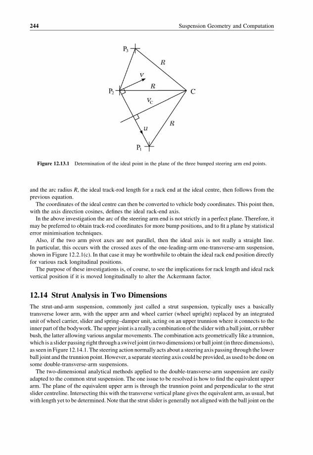
and the arc radius R, the ideal track-rod length for a rack end at the ideal centre, then follows from the

previous equation.

The coordinates of the ideal centre can then be converted to vehicle body coordinates. This point then,

with the axis direction cosines, defines the ideal rack-end axis.

In the above investigation the arc of the steering arm end is not strictly in a perfect plane. Therefore, it

may be preferred to obtain track-rod coordinates for more bump positions, and to fit a plane by statistical

error minimisation techniques.

Also, if the two arm pivot axes are not parallel, then the ideal axis is not really a straight line.

In particular, this occurs with the crossed axes of the one-leading-arm one-transverse-arm suspension,

shown in Figure 12.2.1(c). In that case it may be worthwhile to obtain the ideal rack end position directly

for various rack longitudinal positions.

The purpose of these investigations is, of course, to see the implications for rack length and ideal rack

vertical position if it is moved longitudinally to alter the Ackermann factor.

12.14 Strut Analysis in Two Dimensions

The strut-and-arm suspension, commonly just called a strut suspension, typically uses a basically

transverse lower arm, with the upper arm and wheel carrier (wheel upright) replaced by an integrated

unit of wheel carrier, slider and spring–damper unit, acting on an upper trunnion where it connects to the

inner part of the bodywork. The upper joint is a really a combination of the sliderwith a ball joint, or rubber

bush, the latter allowing various angular movements. The combination acts geometrically like a trunnion,

which is a slider passing right through a swivel joint (in two dimensions) or ball joint (in three dimensions),

as seen in Figure 12.14.1. The steering action normally acts about a steering axis passing through the lower

ball joint and the trunnion point. However, a separate steering axis could be provided, as used to be done on

some double-transverse-arm suspensions.

The two-dimensional analytical methods applied to the double-transverse-arm suspension are easily

adapted to the common strut suspension. The one issue to be resolved is how to find the equivalent upper

arm. The plane of the equivalent upper arm is through the trunnion point and perpendicular to the strut

slider centreline. Intersecting this with the transverse vertical plane gives the equivalent arm, as usual, but

with length yet to be determined. Note that the strut slider is generally not alignedwith the ball joint on the

Figure 12.13.1 Determination of the ideal point in the plane of the three bumped steering arm end points.


lower arm, so not coinciding with the steering axis which passes through the two joints, Figure 12.14.1.

The lower arm angle is uYL, positivewhen the outer ball joint is higher than the axis, but usually negative inthe static position.

The upper arm length can simply be taken effectively as infinite, that is, as having zero shortness.

A slightly better equivalent is to take it to be equal to the swing arm length in front view and the pitch arm

length in side view. In Figure 12.14.2, AB is the lower arm, E is the foot of the perpendicular from B onto

the slider centreline, DE is the slider centreline, and BD is the steering axis through the lower ball joint B

and trunnion centre D. Figure 12.14.2(b) shows the velocity diagram for a lower arm angular velocityW.The fixed points are A and C. The line ab has length value (units m/s)

ab ¼ VLAB

Figure 12.14.1 Strut-and-arm suspension, basic front-view geometry.

Figure 12.14.2 Basic strut-and-arm geometry for analysis of the effective upper arm length.


at the angle c ¼ � uYL. The line cd is perpendicular to CD, and parallel to slider DE. Line bd is

perpendicular to BD. Triangle cbd is similar to CBD. The radius of the movement arc of D, the velocity of

D and the angular velocity of ED are related by

VD ¼ vEDRD

The angular velocity is

vED ¼ ed

LED

The radius of the arc is therefore

RD ¼ VD

vED

¼ cd LED

ed¼ LCD

so the effective centre of the arc is at C, on the line BA, and the effective length of the upper arm is

LYU � RS

Adapting Table 12.8.3 with appropriate modifications for the upper arm gives Table 12.14.1 for the strut-

and-arm suspension lateral properties.

Note that SYD¼ SYU� SYLwill inevitably be negative in practice, so«BC2will be positive.HBJD ismuch

larger than for a conventional double-wishbone suspension.

The longitudinal properties can be analysed in the sameway, with similar adaptations to Table 12.11.1,

giving Table 12.14.2.

Table 12.14.1 Strut-and arm suspension, summary of two-dimensional

lateral equations

«BScd0;Y ¼ 12ðfBJH uYD0� uYS0Þ (12.14.1)

RS ¼ HBJD

uYD0(12.14.2)

«BC1 ¼ � 1

RS

(12.14.3)

SYU ¼ 1

RS

(12.14.4)

«BScd1;Y ¼ 12ðfBJHSYD�SYSÞ (12.14.5)

«BC2 ¼ � SYD

2HBJD

(12.14.6)

Table 12.14.2 Strut-and-arm suspension, summary of two-dimensional

longitudinal equations

«BScd0;X ¼ 12ðfBJH uXD0� uXS0Þ (12.14.7)

RP ¼ HBJD

uXD0(12.14.8)

«Bcas1 ¼ 1

RP

(12.14.9)

SXU ¼ 1

RP

(12.14.10)

«BScd1;X ¼ 12ðfBJHSXD�SXSÞ (12.14.11)

«Bcas2 ¼ SXD

2HBJD

(12.14.12)


12.15 Strut Numerical Solution in Two Dimensions

A computer numerical analysis can be made of the strut-and-arm suspension in two dimensions, using a

geometrically correct solution, without approximations for the upper arm. The technique required is

different from the double-arm suspension. Figure 12.15.1 shows the geometry. AB is the lower arm, with

pivotA and outer ball joint B, ED is the slider axis, at front-view slider initial angle uYSL,with E the foot of

the perpendicular from B. Point F is the wheel contact point.

A preliminary analysis is made of some initial or unchanging lengths and angles, as in Table 12.15.1.

Point B may be inboard or outboard of E, which must be accounted for, for example with a variable IBDE,

effectively representing a sign of angle uBDE. The solution for a given lower arm angle proceeds as in

Table 12.15.2.

When implemented correctly, this is numerically very accurate, although still subject to the two-

dimensional approximations from the real three-dimensional problem. The camber angle and scrub for a

series of lower-arm angles can then be curve fitted against the bump to obtain the various coefficients. The

results may be compared with the results of the analytical method, as in Table 12.15.3.

The comparison shows that the approximated analytic expressions are not very accurate, but do give a

good qualitative estimate and understanding of the consequences of design changes.

Figure 12.15.1 Strut-and-arm geometry for front-view two-dimensional numerical solution.

Table 12.15.1 Strut-and-arm two-dimensional front view, numerical

analysis initial calculations

(1) uYL0 lower arm initial angle

(2) LAB lower arm length

(3) (yE,zE), hence LBE(4) uED0¼p/2� uYSL(5) LFB to the wheel contact point

(6) uFB0 initial angle of FB

(7) IBDE¼ þ 1 or �1 as BD steeper than ED or not

(8) Initial yF0 (half track)


12.16 Strut Design Process

Application of the two-dimensional analytical equations of Table 12.14.1 to design of a strut-and-arm

suspension is very revealing.Whereas the double-arm suspension is very adaptable and can be specified to

give almost any desired coefficients, the strut-and-arm suspension is very limited because of the long

equivalent upper arm. The arm shortness difference

SYD ¼ SYU � SYL

is negative, so the quadratic bump camber coefficient

«BC2 ¼ � SYD

2HBJD

Table 12.15.3 Strut-and-arm comparison of two-dimensional analytic and numerical solutions

Strut-and-Arm, summary comparison table:

Data:

Y Z

Trunnion centre D (m) 0.482 0.710

Lower arm outer B (m) 0.606 0.196

Lower arm length = 0.280 m

Lower arm angle = -1.000 deg

Track = 1.400 m

Slider angle = 16.000 deg

Results:

Analytic Analytic Numerical

LU = LS LU = infinity

eBC1 rad/m -0.577 -0.577 -0.499

eBC2 rad/m2 2.913 3.474 2.075

eBScd0 - - - 0.131 0.131 0.111

eBScd1 m-1 -4.713 -4.933 -4.162

Table 12.15.2 Strut-and-arm two-dimensional front view, numerical

solution, one position

(1) Specify lower arm angular displacement fAB.

(2) uAB ¼ uAB0 þfAB.

(3) Calculate (yB,zB) from yA, zA, LAB and uAB.(4) Obtain LBD (D fixed).

(5) Obtain angle uBD from coordinates of B and D (use atan2).

(6) Obtain uBDE¼ asin (LBE/LBD).

(7) uED ¼ uBD�IBDE uBDE.(8) The bump camber angle is gB ¼ uED� uED0.

(9) Obtain uFB ¼ uFB0 þ gB.(10) Contact point scrub is yF ¼ yB þ LFBcos uFB�yF0.

(11) Contact point bump is zF ¼ zB�LFBsin uFB.


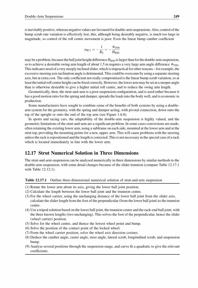
is inevitably positive,whereas negativevalues are favoured for double-armsuspensions.Also, control of the

bump scrub rate variation is effectively lost, this, although being desirably negative, is much too large in

magnitude, so control of the roll centre movement is poor. Even the linear bump camber coefficient

«BC1 ¼ � 1

RS

¼ � uYD0HBJD

maybe aproblem, because theball joint height differenceHBJD is larger than for thedouble-arm suspension,

so to achieve a desirable swing arm length of about 1.5 m requires a very large arm angle difference uYD0.This indicates needof avery steeply inclined slider, which is impractical for other reasons – for example, the

excessive steering axis inclination angle is detrimental. This could be overcomebyusing a separate steering

axis, but at extra cost. The only coefficient not really compromised is the linear bump scrub variation, so at

least the initial roll centre height can be fixed correctly.However, the lower armmay be set at a steeper angle

than is otherwise desirable to give a higher initial roll centre, and to reduce the swing arm length.

Geometrically, then, the strut-and-arm is a poor suspension configuration, and is used rather because it

has a goodmotion ratio for the spring and damper, spreads the loads into the bodywell, and is economic in

production.

Some manufacturers have sought to combine some of the benefits of both systems by using a double-

arm system for the geometry, with the spring and damper acting, with pivotal connection, down onto the

top of the upright or onto the end of the top arm (see Figure 1.6.8).

In sports and racing cars, the adaptability of the double-arm suspension is highly valued, and the

geometric limitations of the strut-and-arm are a significant problem. In some cases conversions are made,

often retaining the existing lower arm, using a subframe on each side, mounted at the lower arm and at the

strut top, providing the mounting points for a new, upper, arm. This will cause problems with the steering

unless the rack is repositioned and the length is corrected. This is not necessary in the special case of a rack

which is located immediately in line with the lower arm.

12.17 Strut Numerical Solution in Three Dimensions

The strut-and-arm suspension can be analysed numerically in three dimensions by similar methods to the

double-arm suspension, with some detail changes because of the slider trunnion (compare Table 12.17.1

with Table 12.12.1).

Table 12.17.1 Outline three-dimensional numerical solution of strut-and-arm suspension

(1) Rotate the lower arm about its axis, giving the lower ball joint position.

(2) Calculate the length between the lower ball joint and the trunnion centre.

(3) For the wheel carrier, using the unchanging distance of the lower ball joint from the slider axis,

calculate the slider length from the foot of the perpendicular (from the lower ball joint) to the trunnion

centre.

(4) Use a tripod solution based on the lower ball joint, the trunnion centre and the rack-end ball joint, with

the three known lengths (two unchanging). This solves the foot of the perpendicular, hence the slider

(wheel carrier) position.

(5) Solve for the wheel centre, and thence the lowest wheel point and bump.

(6) Solve the position of the contact point of the locked wheel.

(7) From the wheel carrier position, solve the wheel axis direction cosines.

(8) Deduce the camber angle, caster angle, steer angle, lateral scrub, longitudinal scrub, and suspension

bump.

(9) Analyse several positions through the suspension range, and curve fit a quadratic to give the relevant

coefficients.


12.18 Double Trailing Arms

The double-trailing-arm system, as shown in Figure 1.6.2, has long been used at the front of small passenger

cars, often with transverse torsion bar springing, sometimes with a spring acting down onto the top arm.

In the common form of this suspension, the two pivot axes are parallel to one another, and perpendicular

to the vehicle centre plane, which gives a very simple geometry. In front view the wheel simply moves

vertically in bump. There is no camber and no lateral scrub. In side view, the trailing arms are parallel,

giving zero caster change. The arms are of the same length, so the quadratic caster coefficient is also zero.

There is quadratic longitudinal scrub.

A more interesting version is also possible, in which modifications are introduced to achieve desired

coefficients. First, in front view, the arm axes may be inclined, Figure 12.18.1.

The lateral length factors are still

LYU ¼ ¥;SYU ¼ 0;SYS ¼ 0;

LYL ¼ ¥SYL ¼ 0

SYD ¼ 0

For double trailing arms, bump action does not alter the equivalent front-view arm angles, so

uYS ¼ uYS0 ¼ uYU0 þ uYL0

uYD ¼ uYD0 ¼ uYU0 � uYL0

Table 12.8.3, previously presented for double transverse arms, is applicable for the lateral properties,

inserting the above length factors, giving the lateral bump scrub and bump camber expressions seen in

Table 12.18.1.

Because the arms are trailing (from the body) they lead from the wheel carrier, so in the terminology

used for general transverse arms the lengths would be negative. To avoid this confusion, the side-view arm

lengths are redefined as positive, as seen in Figure 12.18.2, which also shows positive arm angles, the arm

angle increasing in bump. The lower arm shown has a greater angle, so the pitch arm length is positive, and

the angle included at the pitch centre is positive, so being �uXD0. Because of the redefinition of the armlengths, Table 12.11.1 for transverse arms is not directly applicable.

The pitch arm radius is

RP ¼ HBJD

� uXD0¼ �HBJD

uXD0 þ SXDzS

The pitch centre height is

HP ¼ HBJM þ 1

2uXSRP

Figure 12.18.1 Modified double trailing arms, front view, effective arm length infinite.


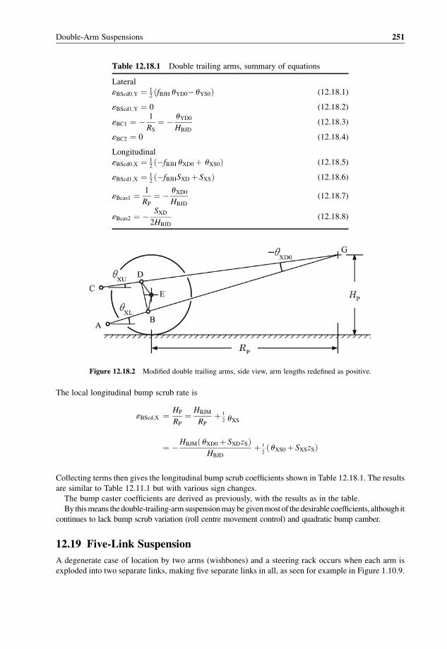
The local longitudinal bump scrub rate is

«BScd;X ¼ HP

RP

¼ HBJM

RP

þ 1

2 uXS

¼ �HBJMð uXD0 þ SXDzSÞHBJD

þ 1

2ð uXS0 þ SXSzSÞ

Collecting terms then gives the longitudinal bump scrub coefficients shown in Table 12.18.1. The results

are similar to Table 12.11.1 but with various sign changes.

The bump caster coefficients are derived as previously, with the results as in the table.

By thismeans thedouble-trailing-armsuspensionmaybegivenmost of the desirable coefficients, although it

continues to lack bump scrub variation (roll centre movement control) and quadratic bump camber.

12.19 Five-Link Suspension

A degenerate case of location by two arms (wishbones) and a steering rack occurs when each arm is

exploded into two separate links, making five separate links in all, as seen for example in Figure 1.10.9.

Table 12.18.1 Double trailing arms, summary of equations

Lateral

«BScd0;Y ¼ 12ðfBJH uYD0� uYS0Þ (12.18.1)

«BScd1;Y ¼ 0 (12.18.2)

«BC1 ¼ � 1

RS

¼ � uYD0HBJD

(12.18.3)

«BC2 ¼ 0 (12.18.4)

Longitudinal

«BScd0;X ¼ 12ð�fBJH uXD0 þ uXS0Þ (12.18.5)

«BScd1;X ¼ 12ð�fBJHSXD þ SXSÞ (12.18.6)

«Bcas1 ¼ 1

RP

¼ � uXD0HBJD

(12.18.7)

«Bcas2 ¼ � SXD

2HBJD

(12.18.8)

Figure 12.18.2 Modified double trailing arms, side view, arm lengths redefined as positive.


This is claimed to offer greater design freedom to obtain some compliance properties, particularly for a

driven wheel. Geometrically, the present problem is to solve for the wheel carrier position as it moves in

bump. In general, analytic methods are not easily applied, because the equations are non-linear and

unwieldy, so an iterative numerical solution is used.

The complete wheel carrier position is specified by six coordinates, say (x, y, z), of a given point,

possibly thewheel centre, and angles ðg; d; uÞ of camber, steer and pitch. From these, the position of each

of the six ball joints on the carrier can be calculated. The lengths of the spaces between these points and the

corresponding points on the body can also be calculated, and compared with the link lengths. The position

variables are then iteratively adjusted to reduce the link length discrepancies to nominally zero.

Normally the vertical position variable z would be specified, leaving five variables to determine. This

can be done cyclically,making a series of passes through the set of variables, each variable being improved

in turn. An increment of the variable is tested, to measure the change in each link space. These are the

influence coefficients for that variable. Thevariable can then be changed tominimise the total discrepancy.

Alternatively, all five variables can be adjusted simultaneously. The influence coefficients of all five

variables are determined together, which then gives five simultaneous equations for the new position

variables.

The values of the influence coefficients found vary somewhat with the carrier position, so there is a need

to re-evaluate them at each step. The second method above is slower per cycle, but becomes strongly

convergent when close to the solution.

The bumpproperties can be investigated in the usualway, by solving for the carrier position at a series of

suspension bumps and then curve fitting quadratic equations. The five-link suspension has all the design

variability of a double-transverse arm, and so can be given any geometric properties desired in practice.

Themethod of solution is similar to that for a rigid axle, which is discussed in some detail in Chapter 13.

————— // —————


13

Rigid Axles

13.1 Introduction

This chapter dealswith rigid axles having rigid link location.A rigid axle is simply defined as one onwhich

the two wheels are physically connected without relative change of position other than a very small

amount of axle compliance. Trailing-twist axles are excluded. Chapter 1 gives diagrams of many

examples of rigid axles. Leaf-spring located axles are typically dealt with by considering an equivalent

link system.

Three basic forms of geometric analysis can be used on a rigid axle: pivot-point analysis; link analysis;

and computer numerical analysis. The purpose of such analysis is to reveal the suspension geometric

characteristics in a similar way to those of an independent suspension. However, the variables used are

different.

13.2 Example Configuration

Figure 13.2.1 shows a general four-link axle in simple line drawing form, similar to the real design shown

in Figure 1.7.3. Lateral location is achieved by the plan-view inclination of the links. In some cases the two

upper linksmeet at the axle, giving a single lateral location point there shared by the two links.More often,

and more practical in construction, the two links may be brought close together but still separate.

In many cases there is single longitudinal upper link, with lateral location provided by a specific-

purpose mechanism. Typically this is laid out horizontally just behind the axle, and is formed of either a

simple Panhard rod or a Watt’s linkage.

In Figure 13.2.1 it is apparent that the wide-spread lower links are likely to be a dominant factor in

controlling the important steer angle of the axle. However, this also depends on the spacing at the front of

the links.

13.3 Axle Variables

For an independent suspension, the fundamental independent variable is the individual suspension bump.

For a rigid axle, there are two basic independent variables. These could be considered to be the suspension

bump values at each of the twowheels, zSBL and zSBR, but more often the complete axle variables are used,

namely the axle suspension heave zAS and the axle suspension roll anglefS. The axle bump ismeasured at

the centre of the axle, so, for small angles, the axle suspension heave (symmetrical double bump) and the


axle suspension roll are given by

zAS ¼ 1

2ðzSBL þ zSBRÞ

fS ¼ fB � fA ¼ zSBR � zSBL

LAx

ð13:3:1Þ

where LAx is the length of the axle between the wheel centres, fB is the body roll angle and fA is the axle

roll angle on the tyres. Correspondingly, the individual wheel suspension bumps left and right are

zSBL ¼ zAS � 1

2LAxfS

zSBR ¼ zAS þ 1

2LAxfS

ð13:3:2Þ

The geometric properties, such as the roll steer coefficients, of the axle are usually expressed in

terms of the suspension heave and roll, but could also be expressed in terms of the two single-wheel

bumps.

A rigid body in three dimensions has six degrees of freedom, these being three displacements and three

angles (expressed, for example, as the Euler angles). In the case of an axle these can be taken as the surge

(X), the sway (Y), the heave (Z), the roll angle (f), the pitch/caster angle (u) and the steer/yaw/heading

angle (d). For an axle, the independent variables are the heave (Z position) and the roll angle, leaving fourvariables to be determined, corresponding to the remaining four degrees of freedom and the four links

constraining the axle.

The displacements are straightforward, in the (X, Y, Z) directions, and performed first. The angles need

to be acted on in a specific order. In general vehicle engineering the Euler angles are normally used, which

are in the order heading angle, pitch angle and roll angle. In the case of an axle, the roll angle is an

independent variable, and best taken first, followed by the steer angle and then the pitch angle. Note that

the axle heave steer angle is not the same as a rigid axlewith steeredwheels, which has independent wheel

steer rotation relative to the axle. The latter also involves the steering mechanism.

The roll angle, taken first, is about an axis parallel to the longitudinal reference X axis, through the axle

centre. The steer angle is then about the vertical Z axis. The pitch angle is last, performed most

conveniently about the axis line between the wheel centres.

Figure 13.3.1 shows the axle centreline AB (the line between the twowheel centres) with roll and steer

angles applied in that order. In the context of a computer analysis, the angles must be related to the

coordinates of the wheel centres A and B, with the angles taken in the correct order. The axle length

Figure 13.2.1 A general four-link axle.


between centres is LAx¼ LAB. AD is parallel to the Y axis, CD is parallel to theX axis and BC is parallel to

the Z axis. Then

LBC ¼ LAx sin f ¼ zB � zC

LCD ¼ LAx cos f sin d ¼ �ðxC � xDÞ ¼ �ðxB � xDÞLAD ¼ LAx cosf cos d ¼ yD � yA ¼ yC � yA ¼ yB � yA

For given wheel centre coordinates, the angles may be deduced from

sin f ¼ zB � zC

LAx

and, with the steer angle positive for right-hand rotation about the Z axis,

tan d ¼ �xC � xD

yD � yA¼ � xB � xA

yB � yA

The axle pitch angle does not arise directly in the above, being applied subsequently about the axle

centreline AB.

Table 13.3.1 summarises the geometric coefficients of an axle, expressed in terms of the suspension

heave and roll, as usual. The single-wheel bump coefficients are easily derived from these, if desired, by

considering a single-wheel bump as a combination of axle heave and roll (equations 13.3.2). This gives a

further set of coefficients for each side separately, possiblywith non-symmetrical values because of design

features (e.g. a Panhard rod) or because of manufacturing tolerance asymmetry. The scrub values are only

really of physical importance at the wheels, but the axle can be considered to have mean effective

coefficients on its centreline.

In all cases there are, in principle, linear and quadratic coefficients (e.g. axle roll steer «ARS0 and «ARS1)

as for independent suspensions, although some of thesemay be rather small, particularly where the design

intent is true lateral symmetry, and often neglected. Examplevalues are given later. Evenmore terms could

be considered, treating each coefficient as a polynomial.

Amongst the first six coefficients of Table 13.3.1, row 4 is of the greatest importance – heave steer and,

particularly, roll steer. The surge, sway and pitch aremainly of significance for their influence on the effect

found at the base of the wheels, reflected in the scrub coefficients. The longitudinal scrub can affect

Figure 13.3.1 Roll and steer angles of an axle defined, taken in that order, AB being the line between the wheel

centres, AD parallel to the Y axis, CD parallel to the X axis, BC parallel to the Z axis. Subsequent pitch is about the axle

centreline AB.

Rigid Axles 255

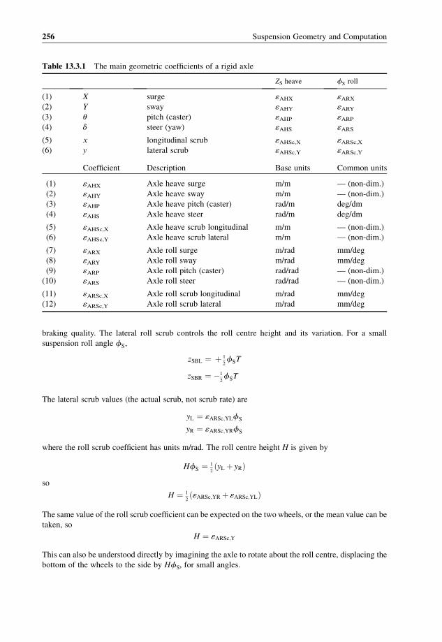
braking quality. The lateral roll scrub controls the roll centre height and its variation. For a small

suspension roll angle fS,

zSBL ¼ þ 1

2fST

zSBR ¼ �1

2fST

The lateral scrub values (the actual scrub, not scrub rate) are

yL ¼ «ARSc;YLfS

yR ¼ «ARSc;YRfS

where the roll scrub coefficient has units m/rad. The roll centre height H is given by

HfS ¼ 1

2ðyL þ yRÞ

so

H ¼ 1

2ð«ARSc;YR þ «ARSc;YLÞ

The same value of the roll scrub coefficient can be expected on the two wheels, or the mean value can be

taken, so

H ¼ «ARSc;Y

This can also be understood directly by imagining the axle to rotate about the roll centre, displacing the

bottom of the wheels to the side by HfS, for small angles.

Table 13.3.1 The main geometric coefficients of a rigid axle

ZS heave fS roll

(1) X surge «AHX «ARX(2) Y sway «AHY «ARY(3) u pitch (caster) «AHP «ARP(4) d steer (yaw) «AHS «ARS

(5) x longitudinal scrub «AHSc,X «ARSc,X(6) y lateral scrub «AHSc,Y «ARSc,Y

Coefficient Description Base units Common units

(1) «AHX Axle heave surge m/m — (non-dim.)

(2) «AHY Axle heave sway m/m — (non-dim.)

(3) «AHP Axle heave pitch (caster) rad/m deg/dm

(4) «AHS Axle heave steer rad/m deg/dm

(5) «AHSc,X Axle heave scrub longitudinal m/m — (non-dim.)

(6) «AHSc,Y Axle heave scrub lateral m/m — (non-dim.)

(7) «ARX Axle roll surge m/rad mm/deg

(8) «ARY Axle roll sway m/rad mm/deg

(9) «ARP Axle roll pitch (caster) rad/rad — (non-dim.)

(10) «ARS Axle roll steer rad/rad — (non-dim.)

(11) «ARSc,X Axle roll scrub longitudinal m/rad mm/deg

(12) «ARSc,Y Axle roll scrub lateral m/rad mm/deg


13.4 Pivot-Point Analysis

Thismethod, previously described inSection 6.12, is described again here for convenient comparisonwith

other methods. It is based on studying the support links to find two points A and B where forces are

effectively exerted by the axle on the body, as in Figure 13.2.1. This assumes that the link lines do in fact

meet, which in reality is not quite the case because ofmanufacturing toleranceswhen in the static position.

Also, when the suspension is rolled, even in the ideal case the lines will no longermeet. The assumption of

the locating points A and B is therefore a useful fiction, an engineering approximation. Kinematically, the

line through points A andB forms a pivot axis for the axle relative to the body.Kinetically, the pointsA and

B are also points at which the lateral forces can be transmitted from the axle to the body, giving the usual

close relationship between the geometric, kinematic and kinetic properties. The line through AB

penetrates the transverse vertical plane of the axle at the geometric roll centre, which in simple analysis

is then also used as the force roll centre.

The axis AB also provides a way to investigate the roll steer characteristics of the axle. For certain

purposes, the vehicle is perceived to roll about the roll axis, joining the roll centres of the front and rear

suspensions. In the present context, however, a roll about such an axis consists of a roll about a horizontal

longitudinal axis and a yawangular displacement. Now, evidently, the yawangle of thewhole vehicle does

not alter the suspension bump steer or roll steer angles. Therefore, to examine the roll steer, the body is

considered to roll about a horizontal longitudinal axis, with a suspension roll angle fS. Whatever the

height of this axis, the lateral displacement of the forward point A relative to the rear point B is

YA=B ¼ �fSðzA � zBÞ

This will create a steer angle of the axle, actually for a rear axle an understeer angle

dUS ¼ YA=B

XA=B

¼ �fS

zA � zB

xA � xB

The corresponding linear roll understeer coefficient of a rear axle is then

«RU1 ¼ � zA � zB

xA � xB¼ rA

where rA is the inclination angle of the axle axis AB expressed in radians (not of the vehicle roll axis). The

effect will be an understeer one when a rear axle has an axis lower at the front point, as shown in the

diagram. For a front axle, understeer occurs for an axis pointing upwards at the front.

Suitable points A and B can be found for other axle link layouts. For example, if the lower links are

parallel then the point A is at infinity, so AB is parallel to the bottom links. If the bottom link pair is

replaced by a torque tube or similar system, then point A is the front ball joint. If transverse location is by a

Panhard rod, then point B is the point atwhich the rod intersects the vertical central plane. AWatt’s linkage

is usually installed with the centre point of the small vertical member attached to the axle, and the outer

ends of the links attached to the body (e.g. Figure 1.7.6).

A characteristic of the Panhard rod is that the roll centre rises for roll in one direction, and falls for the

other, because of vertical motion of the point of connection to the body. For other axle lateral location

systems it is similarly necessary to find the point where the line of action of the force intersects the central

vertical longitudinal plane.

The ‘pivot-point’ method of analysis also gives some insight into the effect of suspension bump

position on the suspension characteristics, and hence into the effect of additional vehicle load. By some

analysis of the suspension details, it is possible, and often easy, to see how the points A and Bwill move

vertically when the axle moves in heave (e.g. when the body lowers due to an extra load). In

Figure 13.2.1 it is apparent that as the body lowers, the front point A will lower, and the rear

Rigid Axles 257

point Bwill rise, for this particular design. This arrangement will tend to keep the roll centre at a fairly

constant height. On the other hand, the inclination of the axis AB will increase with suspension bump

and with load. The result will be an increased linear understeer from the rear axle, and of the linear

understeer of the vehicle. This may be held to be an advantage of the system illustrated, in that a greater

load on the rear of the vehicle has a partially compensating increase of linear understeer. However, the

small vertical change of the roll centre height will not influence the increase of final oversteer due to the

extra load in conjunction with the tyre characteristics. Arguably, then, it may be better to use an

arrangement in which the roll centre is lowered as the load increases, giving preference to the more

critical limit-state handling.

13.5 Link Analysis

The axle characteristics can usefully be investigated by direct analysis of the links, particularly with some

simple configurations. Consider a rigid axle with a single-point upper lateral location and two lower

parallel longitudinal members, along the lines of Figure 1.7.4 or 1.9.1, such that the lower longitudinal

arms govern the steer angle of the axle, as illustrated here in Figure 13.5.1. The longitudinal links are

characterised by their length, static angle to the horizontal, and spacing.

Consider then a body roll giving a suspension roll angle fS on such a system. Relative to the axle, the

front of the left link will rise and the front of the right link will fall. In conjunction with the link static

inclination in side view, this will give a linear roll steer effect. Also, the non-infinite length of the linksmay

give a secondary steer effect.

The resulting understeer angle, dUS, for a rear axle, will be given by

dUS ¼ � dxL� dxR

B

where x is the forwardmovement of the axle point. For a small body roll angle, the left link front end rises,

pushing the axle back, so

dxL ¼ � 1

2BfS uL0

dxR ¼ þ 1

2BfS uR0

dUS ¼ 1

2fSð uR0 þ uL0Þ

Figure 13.5.1 Rigid axle with steer governed by two parallel longitudinal links (other links not shown).


The consequent linear understeer coefficient is therefore

«RU1 ¼ 1

2ð uR0 þ uL0Þ

Considering now links of different lengths, (e.g. due to manufacturing tolerances),

dxL ¼ LLð1� cos uLÞ � LLð 1

2u2LÞ ¼ LL

1

2

12BfS

LL

� �2

giving

dxL ¼ 1

8

B2

LLf2S

Then, in terms of the link shortnesses S¼ 1/L,

dUS ¼ 1

8BðSR � SLÞf2

S

so the resulting quadratic understeer coefficient is

«RU2 ¼ 1

8BðSR � SLÞ

Evidently, then, the first understeer coefficient arises from any difference in the static arm angles, asmight

occur due to manufacturing tolerances or to asymmetrical loading. The second understeer coefficient

arises fromdifferences of the arm lengths,which is just amatter ofmanufacturing tolerance, usually small.

Figure 13.5.2 shows a simple example axle in side view for two cases. The change of axle pitch angle

can be analysed in a very similar way to the analysis of camber angle on an independent suspension. In the

first case, for a bump dz the longitudinal displacement of the end of the link is

dx ¼ dz tan u � dz u

Considering both links then, the change of pitch angle is

du ¼ dxU � dxL

HA

� dz

HA

ð uU � uLÞ

Figure 13.5.2 Example axle side view: (a) surge and pitch location by inclined links; (b) location by links of different

length/shortnesses.

Rigid Axles 259

The result is a linear axle heave pitch coefficient

«AHP1 ¼ uU � uLHA

For links of different lengths, LU and LL, initially horizontal,

dx ¼ L 1� cosdz

L

� �� L 1

2

dz2

L2¼ 1

2S dz2

The pitch angle change is then

D u ¼ SU � SL

2HA

dz2

with a consequent quadratic axle heave pitch coefficient

«AHP2 ¼ SU � SL

2HA

Further analysis along these lines may be applied to obtain the longitudinal scrub of the bottom of the

wheel in bump, which is held to be significant in braking quality on rough roads, as any bump scrub at this

point is likely to cause deterioration of the braking quality.

13.6 Equivalent Links

AWatt’s linkage, designed correctly, produces an exactly straight line of its control point, over a well-

defined range of movement, until the centre link reaches alignment with one of the lateral links. There are

also other straight-line mechanisms that are sometimes used. Also, theWatt’s linkagemay be deliberately

or accidentally imperfect, giving a very large radius of action. In a simple analytic or computer analysis, it

may be convenient to represent such amechanismby a simple equivalent link. The question arises, then, as

to the accuracy of such an equivalent linkage. Such a situation typically arises where an axle has

longitudinal location at each side by a Watt’s linkage, but the only available software has conventional

links. A very long conventional link can be used, but an actual length must be chosen. Consider a radius

arm representingwhat is really a straight line. The equivalent linkwill be placed at the correct angle, so the

linear effect should agree exactly, but therewill be an unreal second-order effect. This would be zero if the

link were infinitely long. The amount of second-order effect depends on the change of angle of the

equivalent link. Representing the angle of the link by an 8-byte real number, the angle is of order 1 radian,

so there will be no effect at all on the numerical solution if the angle change is less than about 10�15

radians. Considering a suspension displacement of 0.100 m, the actual length of the equivalent link needs

to be 1014 m. In practice, it is easy to use a greater length, say 1020 m. With a real number range of 10308,

this still allows accurate computation. The criterion applied here is of course a rather rigorous one, and

from the point of view of engineering accuracy, an equivalent link of say 1000 m would probably be

adequate.

13.7 Numerical Solution

Whatever the configuration, a numerical analysis by computer can obtain the various characteristics of the

axle, provide that suitable software is available, or written for the purpose, and small details, such as the

effect of manufacturing tolerances of mounting points, are also easily investigated.


The basic rigid axle, as in Figure 13.5.1, is mounted on four links. This is the simplest form. Other more

complex types, such as a Watt’s linkage location, require a specialised program or the use of equivalent

links, as discussed earlier.

In principle, this could be solved by writing equations for the link spaces in terms of the axle position

variables, and setting these equal to the physical link lengths. In practice the equationswould be unwieldy,

and non-linear, and iteration would be required for a practical solution. In practice, then, there is really no

way to avoid doing an iterative solution.

The basis of an iterative solution is that there is an existing position, somewhat in error, and a way to

improve that estimated position. Basically this requires the following:

(1) a suitable set of variables representing the axle position;

(2) a way to calculate from those the coordinates of the link connection points;

(3) a calculation of the link length errors;

(4) a way to use the errors to improve the position.

In practice it is convenient to use a ‘reference triangle’ method, to be described here. Using the

PointATinit and PointAT routines described in Chapter 15, a reference triangle can be defined, with all the

axle points being calculated from that. Consider, then, an axle with points defined as follows:

P1, . . .,P4 link connection points on the body;

P5, . . .,P8 corresponding link points on the axle;

P9 mid point of the axle (mean of P10 and P11);

P10 centre of left wheel;

P11 centre of right wheel;

P12 bottom point of the left wheel;

P13 bottom point of the right wheel.

The reference triangle is then, conceptually, rigidly attached to the axle. Various triangles may be used

successfully, but the choice here, for three points forming a right-angled triangle, is

PT1 coincident with P9, the axle centre point;

PT2 on the axle centreline (P10 to P11), at a distance LT from P9 towards P10;

PT3 approximately above PT1, distance LT from P9 and distance H2LT from PT2, with x

coordinate initially at the same coordinate as PT1.

A suitable length for LT is on the same scale as the suspension itself. A value of 1 m allows it to be

omitted from some equations, for computational efficiency, but the equations are then no longer

dimensionally correct. A value of 0.5 m is good. Another possibility is to use half of the axle length,

bringing the second triangle point into coincidence with the left wheel centre.

The triangle is initially defined for the axle in its specified heaved and rolled position, the surge (X),

sway (Y), steer angle (d) and pitch angle (u) yet to be determined. The axlemust subsequently bemoved in

(X, Y, d, u) to satisfy the links without disturbing the heave and roll positions. This is facilitated by the

choice and use of the triangle. Simply displacing the entire triangle in X or Y is not problematic. By

choosing the first triangle point at the axle mid-point, the triangle can be rotated about Z in steer angle

change without interfering with the heave or roll. Finally, by pitching the axle about the axle line P10P11there is again no unwanted disturbance.

At each cycle of the iteration, the position of the axle points with link connections, P5, . . ., P8, arecalculated, using procedure PointAT, the link spaces are calculated, and hence the link length errors are

known.

Rigid Axles 261

Four linear equations can be written for variation of the link space lengths with the axle position

variables (X, Y, d, u). Denoting change of these variables as a 4-vector X gives a matrix equation

DL ¼ CX

whereC is a sensitivitymatrix, actually varying significantly with the axle position. Inmore detail, with X

as the variation of positions,

DL1 ¼ C1;1X1 þC1;2X2 þC1;3X3 þC1;4X4

DL2 ¼ C2;1X1 þC2;2X2 þC2;3X3 þC2;4X4

DL3 ¼ C3;1X1 þC3;2X2 þC3;3X3 þC3;4X4

DL4 ¼ C4;1X1 þC4;2X2 þC4;3X3 þC4;4X4

Now, ideally the known link space errors E1, . . ., E4 will be eliminated, so the desired link space changes

are just the negatives of the errors, giving the matrix equation

CX ¼ �E

Actually, this gives four simultaneous equations for X1, . . ., X4, which when solved indicate the desired

adjustment to the axle position. In practice the result is imperfect because the local sensitivity matrix

varies with axle position, the problem not being truly linear.With revision of the sensitivity matrix at each

cycle, quadratic convergence can be achieved to high accuracy.

The axle movements are conveniently applied to the axle by moving only the reference triangle as

follows:

(1) Translate the complete triangle by the X and Y increments.

(2) Rotate the triangle by the steer angle correction (Z axis).

(3) Rotate the triangle in pitch about the axle wheel-to-wheel centreline.

Note that the axle iterative solution does not actually imply any particular sequence of angles defining

the axle position (e.g. roll before steer before pitch). The final result of this process is simply the axle point

position coordinates. The angle sequence arises subsequently when the coordinate position is interpreted

as a combination of angular displacements.

Rotation of the triangle in steer is easy, Figure 13.7.1, with the Z coordinate playing no part. Given the

initial (X1, Y1),

R ¼ffiffiffiffiffiffiffiffiffiffiffiffiffiffiffiffiX21 þ Y2

1

q

d1 ¼ atanY1

X1

� �

where the initial angle evaluation must obtain the correct quadrant (e.g. in Fortran use atan2). Then

X ¼ R cos ðd1 þ dÞY ¼ R sin ðd1 þ dÞ


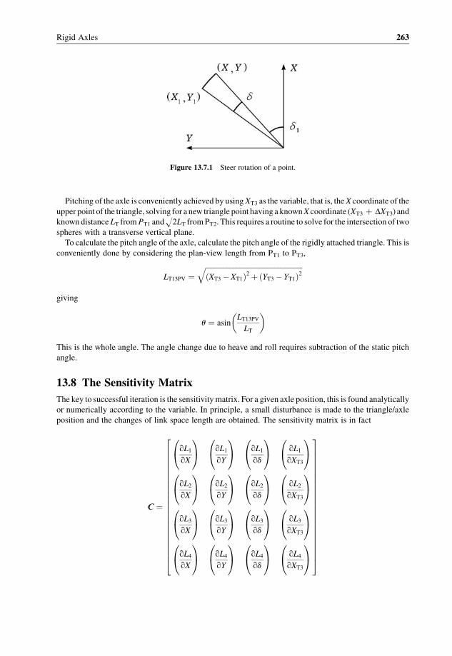
Pitching of the axle is conveniently achieved by usingXT3 as the variable, that is, theX coordinate of the

upper point of the triangle, solving for a new triangle point having a knownX coordinate (XT3 þ DXT3) and

known distanceLT fromPT1 andH2LT fromPT2. This requires a routine to solve for the intersection of two

spheres with a transverse vertical plane.

To calculate the pitch angle of the axle, calculate the pitch angle of the rigidly attached triangle. This is

conveniently done by considering the plan-view length from PT1 to PT3,

LT13PV ¼ffiffiffiffiffiffiffiffiffiffiffiffiffiffiffiffiffiffiffiffiffiffiffiffiffiffiffiffiffiffiffiffiffiffiffiffiffiffiffiffiffiffiffiffiffiffiffiffiffiffiffiffiffiffiffiðXT3 �XT1Þ2 þðYT3 � YT1Þ2

q

giving

u ¼ asinLT13PV

LT

� �

This is the whole angle. The angle change due to heave and roll requires subtraction of the static pitch

angle.

13.8 The Sensitivity Matrix

The key to successful iteration is the sensitivitymatrix. For a given axle position, this is found analytically

or numerically according to the variable. In principle, a small disturbance is made to the triangle/axle

position and the changes of link space length are obtained. The sensitivity matrix is in fact

C ¼

qL1qX

0@

1A qL1

qY

0@

1A qL1

qd

0@

1A qL1

qXT3

0@

1A

qL2qX

0@

1A qL2

qY

0@

1A qL2

qd

0@

1A qL2

qXT3

0@

1A

qL3qX

0@

1A qL3

qY

0@

1A qL3

qd

0@

1A qL3

qXT3

0@

1A

qL4qX

0@

1A qL4

qY

0@

1A qL4

qd

0@

1A qL4

qXT3

0@

1A

26666666666666666666664

37777777777777777777775

Figure 13.7.1 Steer rotation of a point.

Rigid Axles 263

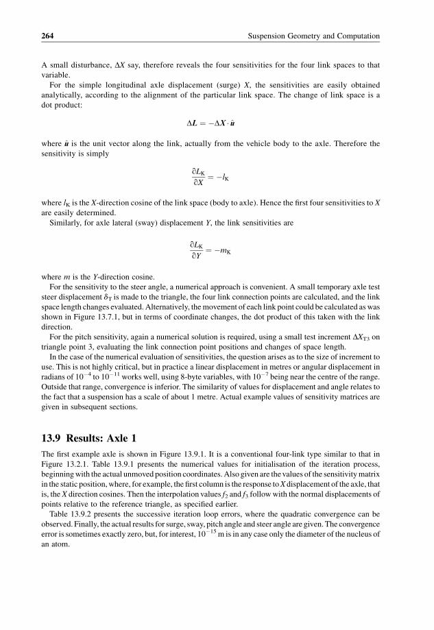
A small disturbance, DX say, therefore reveals the four sensitivities for the four link spaces to that

variable.

For the simple longitudinal axle displacement (surge) X, the sensitivities are easily obtained

analytically, according to the alignment of the particular link space. The change of link space is a

dot product:

DL ¼ �DX � u

where u is the unit vector along the link, actually from the vehicle body to the axle. Therefore the

sensitivity is simply

qLKqX

¼ �lK

where lK is the X-direction cosine of the link space (body to axle). Hence the first four sensitivities to X

are easily determined.

Similarly, for axle lateral (sway) displacement Y, the link sensitivities are

qLKqY

¼ �mK

where m is the Y-direction cosine.

For the sensitivity to the steer angle, a numerical approach is convenient. A small temporary axle test

steer displacement dT is made to the triangle, the four link connection points are calculated, and the link

space length changes evaluated. Alternatively, themovement of each link point could be calculated as was

shown in Figure 13.7.1, but in terms of coordinate changes, the dot product of this taken with the link

direction.

For the pitch sensitivity, again a numerical solution is required, using a small test increment DXT3 on

triangle point 3, evaluating the link connection point positions and changes of space length.

In the case of the numerical evaluation of sensitivities, the question arises as to the size of increment to

use. This is not highly critical, but in practice a linear displacement in metres or angular displacement in

radians of 10�4 to 10�11 works well, using 8-byte variables, with 10�7 being near the centre of the range.

Outside that range, convergence is inferior. The similarity of values for displacement and angle relates to

the fact that a suspension has a scale of about 1 metre. Actual example values of sensitivity matrices are

given in subsequent sections.

13.9 Results: Axle 1

The first example axle is shown in Figure 13.9.1. It is a conventional four-link type similar to that in

Figure 13.2.1. Table 13.9.1 presents the numerical values for initialisation of the iteration process,

beginningwith the actual unmoved position coordinates. Also given are thevalues of the sensitivitymatrix

in the static position,where, for example, the first column is the response toX displacement of the axle, that

is, the X direction cosines. Then the interpolation values f2 and f3 followwith the normal displacements of

points relative to the reference triangle, as specified earlier.

Table 13.9.2 presents the successive iteration loop errors, where the quadratic convergence can be

observed. Finally, the actual results for surge, sway, pitch angle and steer angle are given. The convergence

error is sometimes exactly zero, but, for interest, 10�15 m is in any case only the diameter of the nucleus of

an atom.


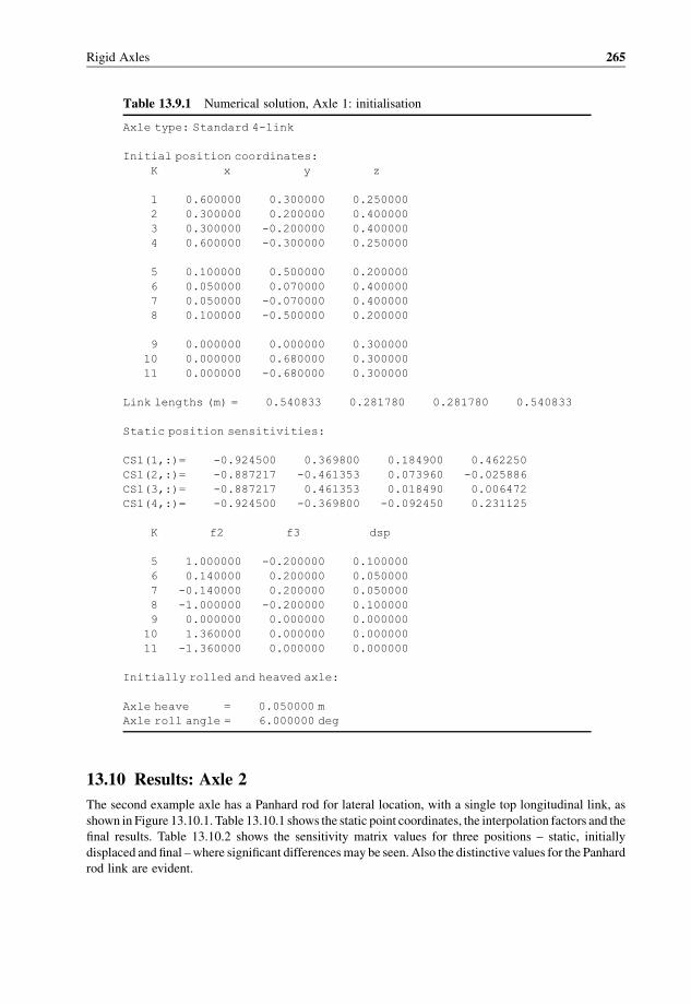
13.10 Results: Axle 2

The second example axle has a Panhard rod for lateral location, with a single top longitudinal link, as

shown in Figure 13.10.1. Table 13.10.1 shows the static point coordinates, the interpolation factors and the

final results. Table 13.10.2 shows the sensitivity matrix values for three positions – static, initially

displaced and final –where significant differencesmay be seen. Also the distinctive values for the Panhard

rod link are evident.

Table 13.9.1 Numerical solution, Axle 1: initialisation

Axle type: Standard 4-link

Initial position coordinates:

K x y z

1 0.600000 0.300000 0.250000

2 0.300000 0.200000 0.400000

3 0.300000 -0.200000 0.400000

4 0.600000 -0.300000 0.250000

5 0.100000 0.500000 0.200000

6 0.050000 0.070000 0.400000

7 0.050000 -0.070000 0.400000

8 0.100000 -0.500000 0.200000

9 0.000000 0.000000 0.300000

10 0.000000 0.680000 0.300000

11 0.000000 -0.680000 0.300000

Link lengths (m) = 0.540833 0.281780 0.281780 0.540833

Static position sensitivities:

CS1(1,:)= -0.924500 0.369800 0.184900 0.462250

CS1(2,:)= -0.887217 -0.461353 0.073960 -0.025886

CS1(3,:)= -0.887217 0.461353 0.018490 0.006472

CS1(4,:)= -0.924500 -0.369800 -0.092450 0.231125

K f2 f3 dsp

5 1.000000 -0.200000 0.100000

6 0.140000 0.200000 0.050000

7 -0.140000 0.200000 0.050000

8 -1.000000 -0.200000 0.100000

9 0.000000 0.000000 0.000000

10 1.360000 0.000000 0.000000

11 -1.360000 0.000000 0.000000

Initially rolled and heaved axle:

Axle heave = 0.050000 m

Axle roll angle = 6.000000 deg

Rigid Axles 265

13.11 Coefficients

By solving for a range of points through the suspension range and fitting a quadratic curve, the basic

coefficients may be obtained. This has been done herewith 11 points for heave through a range�0.100 m

to þ 0.100mand for roll from�0.100 rad to þ 0.100 rad. The results are given in Table 13.11.1 forAxle 1

andTable 13.11.2. forAxle 2.Asmaybe seen in both tables, for the pitch angle the quadratic fit is poor, and

a much higher order of polynomial is required for a really good fit, but the pitch angle is relatively small.

The quadratic fit for the important steer angle is good. Axle 1 is symmetrical, so heave has exactly zero

Figure 13.9.1 ExampleAxle 1,with convergent link location: (a) sideview; (b) front view; (c) planview; (d) axometric

three-quarter view.

Table 13.9.2 Axle 1: iteration results

Iteration loop errors:

Loop Link1 Link2 Link3 Link4 Total abs

0 0.317E-02 0.107E-01 -0.132E-02 -0.458E-02 0.198E-01

1 0.167E-03 0.395E-03 0.250E-03 0.106E-03 0.917E-03

2 0.162E-06 0.429E-06 0.299E-06 0.117E-06 0.101E-05

3 0.172E-12 0.496E-12 0.372E-12 0.134E-12 0.117E-11

4 -0.111E-15 -0.555E-16 0.555E-16 0.000E+00 0.222E-15

Values obtained:



Axle surge = 0.002335 m

Axle sway = 0.011737 m

Axle pitch/caster = 0.185575 deg

Axle steer = -0.922967 deg


Table 13.10.1 Numerical solution, Axle 2: initialisation and iteration

Axle type: One top link, Panhard rod

Initial position coordinates:

K x y z

1 0.600000 0.500000 0.250000

2 0.300000 0.000000 0.500000

3 -0.100000 -0.400000 0.350000

4 0.600000 -0.500000 0.250000

5 0.100000 0.350000 0.200000

6 0.050000 0.000000 0.500000

7 -0.100000 0.400000 0.320000

8 0.100000 -0.350000 0.200000

9 0.000000 0.000000 0.300000

10 0.000000 0.680000 0.300000

11 0.000000 -0.680000 0.300000

Link lengths (m) = 0.524404 0.250000 0.800562 0.524404

K f2 f3 dsp

5 0.700000 -0.200000 0.100000

6 0.000000 0.400000 0.050000

7 0.800000 0.040000 -0.100000

8 -0.700000 -0.200000 0.100000

9 0.000000 0.000000 0.000000

10 1.360000 0.000000 0.000000

11 -1.360000 0.000000 0.000000

Initially rolled and heaved axle:



Iteration loop errors:

Loop Link1 Link2 Link3 Link4 Total abs

0 -0.345E-02 0.559E-02 -0.246E-02 0.253E-02 0.140E-01

1 0.726E-04 0.811E-04 -0.122E-04 0.732E-04 0.239E-03

2 0.111E-07 0.259E-07 0.339E-08 0.115E-07 0.519E-07

3 -0.111E-15 0.167E-14 0.111E-15 0.000E+00 0.189E-14

4 -0.111E-15 0.000E+00 0.000E+00 0.000E+00 0.111E-15

Values obtained:



Axle surge = 0.001558 m

Axle sway = 0.003950 m

Axle pitch/caster = 0.088394 deg

Axle steer = 0.811626 deg

Rigid Axles 267

steer and sway effects, but some heave–steer and heave–sway effectsmay be seen onAxle 2 because of the

Panhard rod lateral location.

Table 13.11.3 presents the quadratic scrub coefficients found for the two axles. Axle 1 is exactly

symmetrical, so heave causes zero lateral scrub. There is significant longitudinal scrub which could be

designed out by adjusting the lateral view link angles. Roll causes 0.0356m/rad linear longitudinal scrub,

Table 13.10.2 Axle 2 sensitivity matrices

Static position sensitivity matrix:

CS1(1,:)= -0.953463 -0.286039 0.190693 0.333712

CS1(2,:)= -1.000000 0.000000 -0.114416 0.000000

CS1(3,:)= 0.000000 0.999298 0.003814 -0.038139

CS1(4,:)= -0.953463 0.286039 -0.066742 0.116799

Starting sensitivity matrix:

CS(1:) = -0.953463 -0.269762 0.172102 0.316961

CS(2:) = -1.000000 -0.083623 -0.411128 -0.024538

CS(3:) = 0.000000 0.993949 -0.005466 -0.099701

CS(4:) = -0.953463 0.309628 0.209821 -0.289556

Final sensitivity matrix:

CS(1:) = -0.963421 -0.259312 0.178379 0.322722

CS(2:) = -0.979243 -0.064430 -0.411390 -0.023097

CS(3:) = -0.004605 0.996852 -0.004667 -0.103098

CS(4:) = -0.944616 0.320211 0.212084 -0.284411

Figure 13.10.1 Example Axle 2, with Panhard rod lateral location: (a) side view; (b) front view; (c) plan view;

(d) axometric three-quarter view.


closely associated with the roll steer which without any pitch effect would give 0.05256� 1.36/2 ¼0.0357m/rad, in good agreement. The linear lateral scrub coefficient in roll is 0.395m/rad, giving the roll

centre height.

For Axle 2, with the Panhard rod, the longitudinal heave scrub happens to be similar to Axle 1, but the

quadratic coefficients are much greater, and there is considerable asymmetry. There is some lateral heave

effect. Roll causes an approximately antisymmetrical linear longitudinal scrub. The linear lateral scrub

with roll averages 0.361m/rad, giving the roll centre height.

Table 13.11.2 Basic heave and roll coefficients for Axle 2

Quadratic fit coefficient matrix:

C0 C1 C2 Q fit

Heave:

Surge -0.000060 -0.070559 1.354386 0.973089

Sway 0.000028 0.041053 -0.751124 0.986469

Pitch 0.005208 0.403181 0.373187 0.784783

Steer 0.000043 0.040367 -0.728536 0.989236

Roll:

Surge -0.000001 0.000120 0.152865 0.993947

Sway 0.000000 0.060982 0.113727 0.999640

Pitch -0.000010 0.000138 0.013249 0.815758

Steer -0.000002 0.260935 0.108252 0.999043

Table 13.11.1 Basic heave and roll coefficients for Axle 1

Quadratic fit coefficients:

C0 C1 C2 Q fit

Heave:

Surge -0.000065 -0.054334 1.497510 0.968790

Sway 0.000000 0.000000 0.000000 - - - - - –

Pitch 0.008868 0.496882 1.345168 0.765415

Steer 0.000000 0.000000 0.000000 - - - - - –

Roll:

Surge 0.000000 0.000000 0.101814 0.999431

Sway 0.000000 0.095631 0.000000 0.999765

Pitch -0.000020 0.000000 0.025374 0.840332

Steer 0.000000 -0.052557 0.000000 0.997766

Rigid Axles 269

————— // —————

Table 13.11.3 Scrub coefficients for Axles 1 and 2

Axle 1 Scrub coefficients:

Heave (units m/m = - - - ):

Left X = 0.000015 -0.196137 0.022234

Right X = 0.000015 -0.196137 0.022234

Left Y = 0.000000 0.000000 0.000000

Right Y = 0.000000 0.000000 0.000000

Roll (units m/rad):

Left X = 0.000000 0.035612 0.322117

Right X = 0.000000 -0.035612 0.322117

Left Y = 0.000000 0.395191 -0.340655

Right Y = 0.000000 0.395191 0.340655

Axle 2 Scrub coefficients:

Heave (units m/m = - - –):

Left X = -0.000018 -0.194421 0.832917

Right X = 0.000040 -0.139523 -0.157875

Left Y = 0.000021 0.041400 -0.749998

Right Y = 0.000017 0.041117 -0.745286

Roll (units m/rad):

Left X = 0.000000 -0.175865 0.257751

Right X = -0.000001 0.177716 0.404189

Left Y = -0.000001 0.360889 -0.248543

Right Y = 0.000000 0.361160 0.477119


14

Installation Ratios

14.1 Introduction

The dynamic behaviour of a vehicle depends on the on the effect of the spring as seen at the wheel,

commonly called the ‘wheel rate’ or ‘effective spring stiffness’, and on the damping coefficient effective at

thewheel. However, the spring and damper are not installed at this point, but elsewhere on the suspension.

The effective spring and damper characteristic at thewheel must therefore be related to the characteristics

of the actual spring and damper. On a double-wishbone suspension they often operate about half-way out

on the bottom suspension arm. On a racing car, often they operate through a linkage, including various

forms of intermediate rocker. Basically the effect of the spring and damper depends on the ratio of

velocities spring-to-wheel and damper-to-wheelwhen thewheel is displaced in its bumpaction. In general

this velocity ratio, also known as the ‘motion ratio’ or ‘installation ratio’, is not a constant, but varies with

thewheel bump position. Analysis of the effect of installation of the spring and damper therefore involves:

(1) evaluation of the relative motion of the spring, damper and wheel,

(2) consideration of the implications of this ratio.

Evaluation of themotion ratio is not too critical, especially in the early stages of design, so approximate

methods, within 1 or 2 per cent, are of some value, and algebraic methods have the benefit of giving

more insight into a design than do numerical methods. Hence the following sections describe algebraic or

drawing methods for common suspensions. These methods may also be used as the basis of computer

programs, as an alternative to the common finite increment of displacement method, or to the numerical

velocity-diagram method.

The main principle involved is the geometry of the lever, or rocker. Rigid-arm suspensions, such as

trailing arms or swing axles, follow on the same principle. Double wishbones require a different kind of

analysis, to relate thewheelmotion to themotion of the end ball joint of the relevant arm, usually the lower

one, which is carrying the spring or damper, giving the first factor of the total motion ratio. Once this is

known, normal rocker analysis will give the other factor. For struts, a slightly different analysis is required.

14.2 Motion Ratio

The main notation required here is as in Table 14.2.1. Note that the subscript K is used for the spring

because the subscript S has already been allocated to ‘suspension’.

At a given suspension bump position zS from static ride height, the spring compression is xK relative to

static. A small further suspension bumpmotion dzS results in a corresponding further spring compression


dxK, Figure 14.2.1. The ratio of these is the displacement motion ratio for the spring at the suspension

bump position zS. This is denotedRK/S (spring relative to suspension bump), generally abbreviated to RK:

RK=S ¼ dxKdzS

Note that this is the spring compression increment divided by the suspension bump increment, not vice

versa. It is the suspension bumpmovement that is considered to be the reference movement. This value of

RK will be independent of zS and dzS only if the system is linear, that is, if the motion ratio RK is constant,

which is generally not true. Therefore, in general the above expression is usable only for small dzS.With a

suitable computer program to analyse the suspension geometry, the motion ratio may be evaluated in the

above way, with dzS being given a suitable small value (e.g. 0.1mm), depending on the precision with

which the suspension position can be calculated. It is the actual suspension position that is solved for each

of the adjacent conditions.

Mathematically, the motion ratio value is really the above ratio as dzS tends to zero. The result, in thelimit, is the derivative

RK ¼ dxK

dzS

This provides a possible means of evaluation if an explicit algebraic expression is available for spring

compression xK as a function of suspension bump displacement zS. For example, if it is known that, over

Table 14.2.1 Main nomenclature for motion ratios

LD m damper length

LK m spring length

RD — damper motion ratio

RK — spring motion ratio

VD m/s damper compression velocity

VK m/s spring compression velocity

VP m/s velocity of intermediate pushrod

VS m/s suspension bump velocity (wheel)

xD m damper compression from static

xK m spring compression from static

zS m suspension bump

Figure 14.2.1 Spring compression displacement v. suspension bump displacement.


the range of interest, the spring compression, perhaps by an empirical curve fit, is

xK ¼ A1zS þ A2z2S

then

RK ¼ dxK

dzS¼ A1 þ 2A2zS

The derivative definition of RK may be extended by inserting a time element:

RK ¼ dxK

dt� dt

dzS

The terms on the right-hand side are a velocity and a reciprocal velocity, so RKmay bewritten as a ratio of

velocities:

RK ¼ VK

VS

The spring motion ratio is therefore identically equal to the quotient of spring compression velocity over

suspension compression (bump) velocity. Because the numerator and denominator are both velocities, the

quotient is dimensionless, and correctly called a ratio.

The velocity ratio definition provides a practical means of evaluating RK if the velocity diagram can be

drawn. Frequently this is feasible, even easy, for a two-dimensional set-up, and may also be practical for a

three-dimensional suspension layout if the parts can be treated sequentially as two-dimensional parts (e.g.

a racing suspension with pushrod and rocker, in many cases). Even a three-dimensional velocity diagram

can be ‘drawn’ by computer. In a direct velocity-diagram solution of the suspension, the single actual

suspension position is used, and the velocities are obtained directly at the actual suspension position; there

is no question of an increment of position. In amanual solution, thevelocity diagrammay indeed be solved

by accurate drawing, but equally if not better by sketching and algebraic solution.

Considering the displacement xP of an intermediate pushrod, the overall springmotion ratio RKmay be

expressed as

RK ¼ dxKdzS

¼ dxKdxP

� dxPdzS

or, in the limit, it is the derivative product

RK ¼ dxK

dxP� dxPdzS

¼ RK=P �RP=S

so the overall motion ratio is the product of the sequential ratios. By induction, this obviously extends to

any number of sequential ratios. In terms of the velocities VK, VP and VS,

RK ¼ VK

VS

¼ VK

VP

� VP

VS

or, more generally, for multiple ratios in sequence

RK ¼ VK

VP1

� VP1

VP2

� � � � � VP;N�1

VP;N� VP;N

VS

Installation Ratios 273

Hence a suspension mechanism can be solved by separate analysis of the sequential parts. This may be

especiallyvaluablewhere a complex suspensioncanbe treated as separate sub-mechanisms, eachanalysable

in two-dimensional motion, and each analysed in the most convenient way for that particular part.

In general the spring or damper motion ratio is not uniform through the bumpmotion, it is a function of

zS, the bump position of the suspension:

RK � RKðzSÞFor passenger cars the value may be approximately constant or may increase slightly with bump, in

the latter case usually also reducing with droop. For racing cars a rather rapidly increasing velocity ratio

may be used.Where applied to a spring, this gives a rising stiffness with bump, and is called a ‘rising-rate’

suspension. Applied to a damper, it is rising-rate damping. Obtaining rising rate by mechanism design

is generally much easier and more controllable than doing so by manufacturing rising rate springs or

position-dependent dampers. Often the spring and damper are fitted co-axially and have the same motion

ratio. For rising rate, this conveniently gives the desirable increase of wheel damping coefficient with

increasing wheel rate. However, a rising rate motion ratio has a different effect on springs from that on

dampers, as discussed in Sections 14.14 and 14.15.

14.3 Displacement Method

One of the ways to obtain the motion ratio value for a given nominal suspension bump position is by

analysis of a pair of slightly different suspension positions. If the position analysis is undertaken by a

drawing method it is prone to inaccuracy because of the relatively small difference of positions. Hence,

the drawing must be undertaken by an experienced draughtsman at a large scale. With less emphasis on

accuracy, a wide spread of the two positions will give an average ratio over the movement which may be

useful in some cases. Also a sequence of, say, eight to ten positions may be drawn throughout the bump

motion, and the damper compression plotted as a graph against suspension position, with the curve

smoothed through the points. This helps to reveal any errors. The spring motion ratio for any particular

position is then the gradient dxK=dzS of the curve at the particular suspension bump position.

Drawingmethods were the traditional technique in bygone days, but are regarded as somewhat archaic

nowadays because of the availability of computers. However, drawingmethodsmay still be of somevalue,

for example if the particular configuration cannot be handled by existing software. In that case, careful

drawing or velocity diagram analysis may be more expedient than writing new software, unless the

configuration is known to be one of lasting interest. Computer-aided drawing packages offer potentially

enhanced accuracy, of course, and can even be used to solve simple installation ratio problems.

In some cases the position relationships may be found algebraically. In three dimensions the solutions

are too unwieldy for hand solution in other than isolated cases, for example to check early results of a

computer analysis. However, if the system can be treated in a two-dimensional sequence then an analytical

expression for positions may be possible, with differentiation giving the velocity ratio.

On one occasion the author was asked to adjudicate between two commercial computer programs

which gave substantially different results. A careful drawing solution clearly sided with one of the two

programs, and also suggested the reason for the fault in the other program. Drawing methods may

therefore still be of value, even in this computerised day and age.

The actual solution of a given suspension position for a given body position (heave, roll and pitch) and

suspension bump due to road displacement and tyre compression requires two- and three-dimensional

coordinate geometry (analytical geometry), discussed in later chapters.

14.4 Velocity Diagrams

Avelocity diagram is a coordinate diagram onwhich any point corresponds to a given velocity, drawn to a

particular velocity scale (e.g. 10mm/s : 1mm). Hence, any point (X, Y) on any component has a velocity


(VX, VY) which can be plotted on the diagram at a point (VX, VY) using a suitable scale; in practice this is

done for a few special points, essentially those at the joints between components, that is, at the pivot points

and at sliders, at the ball joints in a suspension. The distances between points in the velocity diagram

represent velocitymagnitudes. The positionof one point relative to another represents the relativevelocity.

The velocity diagram can be said to be drawn in ‘velocity space’. The velocity diagram is constructed

sequentially, point by point, according to the particular mechanism. It may drawn accurately to a given

scale, or, oftenmoreconveniently andmoreaccurately, simply sketchedand solvedalgebraically.Accurate

drawing requires some numerical calculation anyway. A full description of the principles of velocity

diagram construction appears in standard texts (see the references at the end of this chapter).

Velocity diagrams are usually two-dimensional (VX, VY), corresponding to common two-dimensional

mechanisms, which have point positions (X, Y). Hence, they can be drawn on a two-dimensional surface,

such as a piece of paper. Solution may be by geometrical drawing constructions, or by sketching and

algebra with coordinate geometry.

However, three-dimensional velocity diagrams are also possible conceptually, although difficult to

draw by hand, but can be represented in a computer by three-dimensional velocity vectors (VX, VY, VZ)

obtained algebraically. This can even be extended to three-dimensional acceleration diagrams.

Velocity diagrams and displacement methods for obtaining spring and damper motion ratios are

independent methods, and may be used to provide a check on each other.

14.5 Computer Evaluation

Commercial and proprietary packages are available for analysing suspension geometry on computers. At

least one program, by the author, includes design facilities to specify, for example, a given bump steer for

which the computer will choose suitable link dimensions.

When such numerical analysis packages work, they generally work well and accurately. However, not

all packages can handle all possible configurations, especially for the more esoteric types used in racing.

Also the ‘assembly logic’ of some packages is not always reliable, so that in some configurations there is

a sudden total failure, usually manifested by a ‘square root of negative number’ error (see Chapter 16).

A full three-dimensional analysis program to obtain themotion ratios is a considerable job towritewell.

Such a program is certainly very useful, but provides specific numbers rather than design insight, and is

best considered as an adjunct to qualitative understanding and simple algebraic models rather than

completely replacing them.

14.6 Mechanical Displacement

If the suspension to be analysed already exists, or it is viable to construct one, perhaps adapting some other

design, then it may be useful to actually measure the displacement graph of spring position and damper

position against bumpposition, using dial gauges. This graphmaybe comparedwith solutions achieved by

drawing, analytical methods or computers. The results are likely to be disappointing in some cases. Fair

agreement is usually obtained for passenger cars, but in the case of racing cars, with long links and stiff

springs, the elasticity of suspension members and even of the chassis at the mounting points may give rise

to substantial discrepancies. In that case, if it is accepted that the discrepancy is indeed due to compliance

in the suspension, then a more elaborate suspension model may be required. Figure 14.6.1 shows such a

model, in which the suspension linkage compliance KL is included. Under dynamic conditions, the

suspension bump deflection

zS ¼ zW � zB

is no longer related directly to the spring deflection by a simple geometric motion ratio. However, for a

given static position there are particular loads and deflections, so there is still a definite relationshipxK(zS).


Figure 14.6.1 assumes that the suspension spring and damper operate at the same point, as indeed is

applicable for most racing cars, or else more than one suspension compliance must be included. In a static

position, the damping forces are zero, and the link and suspension spring stiffnesses act in series.

The results of a motion ratio analysis must therefore be applied with some caution for more compliant

suspensions. Even then, however, the motion ratio provides basic insight into the springs and dampers

required, and into the design of a mechanism for rising rate.

14.7 The Rocker

The basic component inmotion ratio evaluation is the rocker, or lever, which arises in principle, even if not

explicitly as a rocker, in virtually all suspensions. In some cases, especiallymodern racing cars, a rocker is

included as such to link the basic suspension to the spring and damper. By virtue of including a pushrod, or

pullrod, and rocker, the spring and damper can be better positioned, vertically inside the body, or, as is

common nowadays, laid down horizontally on top of the body or along the upper sides of the gearbox. This

improves the aerodynamics by removing the spring–damper unit from the high-speed airflow, and the

inclusion of a rocker in the systemmakes it very easy to change the motion ratio and rising rate simply by

changing the rocker.

The function of a rocker, illustrated in Figure 14.7.1, can be specified by three aspects:

(1) the total rocker angular deviation between pushrods, uRD;

(2) the rocker motion ratio, RR;

(3) the rocker rising rate factor, fR.

The rocker shown in Figure 14.7.1 is a completely general one. There are numerous simpler special

cases. The angle uRD is the rocker deflection angle, the total angular difference between input and output,

which will actually vary a little over the range of motion, and is specified at the normal ride height.

Figure 14.6.1 Heave-only suspension model including link compliance KL, which could alternatively be placed

above the KW/CW components.


Figure 14.7.2 shows three examples of deflection angle uRD (0�, 90�, 180�). Intermediate deflection angles

are equally possible.

The rocker motion ratio RR, specified at the normal ride height, depends most obviously upon the arm

lengths from the pivot axes to the input and output points, but also depends on the angular position of the

input and output rods. Figures 14.7.3 and 14.7.4 illustrate some possible ways of achieving motion

ratios V2/V1.

Figure 14.7.1 General rocker configuration: (a) geometry; (b) velocity diagram.


The rising rate of a rocker is the proportional increase of motion ratio per unit of rocker rotation:

fR ¼ 1

RR

� dRR

duR

To express this in terms of suspensionmotion at thewheel (i.e. as wheel rising rate), the geometry of the

rest of the suspensionmust be known, sowheel rising rate is not necessarily a property of the rocker alone,

Figure 14.7.2 Simple rockers with various deflection angles.

Figure 14.7.3 Simple rockers with various motion ratios.

Figure 14.7.4 Simple rockers with various rising rates (zero in the first case).


but becomes so if the rest of the system is essentially linear. When a rising rate is desired, the design

method commonly applied in practice is to guess at some dimensions and then to play with them on the

computer. What is needed is a systematic design procedure.

The properties of the rocker may be deduced for special cases, as required, but in fact can be derived for

the general rocker of Figure 14.7.1 quite easily, by virtue of an informed choice of representational

parameters, arrived at by experience. It is assumed in the following analysis that themotion is planar. If the

input or output rods are not parallel to the rocker plane, defined as a plane perpendicular to the axis of

rotation of the rocker on the body, then the velocities in Figure 14.7.1 are the rocker plane velocities,

related to the actual rod velocities by the cosine of the out-of-plane angle.

The parameters in Figure 14.7.1 are:

(1) the rocker included angle fR, positive when the output leads the input as shown;

(2) the input and output rocker arm lengths l1 and l2;

(3) the input and output rod offset anglesc1 andc2, between the rod and the tangent perpendicular

to the corresponding arm radius;

(4) the rocker position uR, from some appropriate datum, usually the normal ride position;

(5) the input and output rod velocities, in the rod directions, V1 in and V2 out;

(6) the rocker angular velocity vR.

Of the above, lengths l1 and l2 are constant, as isfR, these three parameters being the essence of the rocker

geometry. Other parameters will vary, although vR is normally deemed to be some constant value for the

purpose of analysis.

The performance parameters of the rocker, uRD, RR and fR, are derived as follows. The rocker deviation

angle is

uRD ¼ c1 þfR þc2

In practice, for design purposes, this is required in the form

fR ¼ uRD �c1�c2

Figure 14.7.1(b) is the velocity diagram for the rocker. At rocker angular speed vR, assumed for analysis,

the tangential speed of point A is vRl1, perpendicular to line AC, so at angle uR from the vertical, giving

point a representing VA. Similarly, point b, representing VB, is established at uRþfR.

ThevelocityofAcanberesolvedintocomponentsparallel andperpendicular to the inputrodatangleu1 tothevertical. To do this, construct in the velocity diagram the line at u1 from thevertical, parallel to the input

rod, and drop the perpendicular from a, giving point p. The length cp represents the velocity along the rod,

whilst pa represents the tangential velocity of one end relative to the other. Similarly for the output, so the

actual damper compression speed on the output is represented by cq.The rockermotion ratioRR is given by

RR ¼ VQ

VP

¼ cq

cp

Hence the velocity ratio of the rocker, defined by

RR ¼ V2

V1

is given by

RR ¼ vRl2ð uR þfR� u2ÞvRl1cosð uR þ u1Þ


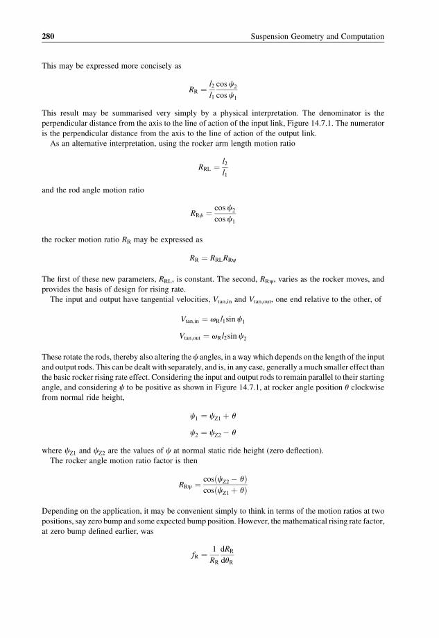
This may be expressed more concisely as

RR ¼ l2

l1

cos c2

cos c1

This result may be summarised very simply by a physical interpretation. The denominator is the

perpendicular distance from the axis to the line of action of the input link, Figure 14.7.1. The numerator

is the perpendicular distance from the axis to the line of action of the output link.

As an alternative interpretation, using the rocker arm length motion ratio

RRL ¼ l2

l1

and the rod angle motion ratio

RRc ¼ cos c2

cos c1

the rocker motion ratio RR may be expressed as

RR ¼ RRLRRy

The first of these new parameters, RRL, is constant. The second, RRy, varies as the rocker moves, and

provides the basis of design for rising rate.

The input and output have tangential velocities, Vtan,in and Vtan,out, one end relative to the other, of

Vtan;in ¼ vRl1sin c1

Vtan;out ¼ vRl2sin c2

These rotate the rods, thereby also altering the c angles, in a waywhich depends on the length of the input

and output rods. This can be dealt with separately, and is, in any case, generally amuch smaller effect than

the basic rocker rising rate effect. Considering the input and output rods to remain parallel to their starting

angle, and considering c to be positive as shown in Figure 14.7.1, at rocker angle position u clockwise

from normal ride height,

c1 ¼ cZ1 þ u

c2 ¼ cZ2 � u

where cZ1 and cZ2 are the values of c at normal static ride height (zero deflection).

The rocker angle motion ratio factor is then

RRy ¼ cosðcZ2 � uÞcosðcZ1 þ uÞ

Depending on the application, it may be convenient simply to think in terms of the motion ratios at two

positions, say zero bump and some expected bump position. However, themathematical rising rate factor,

at zero bump defined earlier, was

fR ¼ 1

RR

dRR

duR


with

RRy ¼ RRy0ð1þ fR uÞThe rocker angle motion ratio at u is

RRy ¼ cosðcZ2� uÞcosðcZ1� uÞ

The rising rate factor fR is given by

fR ¼ 1

u

RRy

RRy;0�1

� �

which, by considering infinitesimal u, with substitution and condensation, becomes

fR ¼ tan c1 þ tan c2

Hence, the rising rate is governed by the angles c1 and c2. Note that these are positive as defined in

Figure 14.7.1 and the signs must be respected; also they may well change sign within the range of motion

of the rocker. Physically, the reason for the rising rate is simply that the input moment arm is increasing,

and the output one is decreasing.

At rocker deflection u the motion ratio RR is therefore estimated to be

RR ¼ RRLRRyð1þ fR uÞ

This method of rising rate analysis is useful for a preliminary appraisal, giving a first estimate of the

required values for c1 and c2 in combination, which then, in conjunction with the required rocker angular

deflection uRD, gives the rocker included angle

fR ¼ uRD�c1�c2

Practically, because of the packaging problems of large rockers, fairly large rocker angularmovements are

used in practice, so once a first estimate has beenmade it is more practical toworkwith two ormore actual

rocker positions, for example normal ride height and a bump position, and to obtain two corresponding

values of motion ratio.

The usual situation is that a given increase of ratio is required for a given rocker angular displacement,

estimated from a given wheel bump motion, intermediate ratio and rocker input arm length. The required

increase of rate may be shared between input and output. The required increase of rate on the input, say, is

then known. Let the ratio be r¼R2/R1. From the angle motion ratio

RRy ¼ cosðcZ2 � uÞcosðcZ1 þ uÞ

may be obtained

r ¼ cos cZ1

cosðcZ1 þ uÞThis may be solved for cZ1 as

tan cZ1 ¼1

sin ucos u� 1

r

� �


giving the correct initial angular position for the arm. In practice it may be difficult to obtain a low enough

ratiowith a practical rocker size, and cZ1 may be negative. This gives a rate which will fall slightly before

then rising to the required value.

For design purposes, rocker design is a matter of juggling the lengths and angles according to the given

input pushrod motion and the required rising rate. Two points to bear in mind are that basically it is the

square of the motion ratio that controls the effect seen at the wheel, and that a motion ratio rising from

normal ride height will also generally fall when below the normal ride height. Hence, large motion ratio

changesmust be designedwith caution. Rising rate also causes an important additional stiffness term even

with a linear spring (see Section 14.14).

14.8 The Rigid Arm

Rigid-arm suspensions, such as a trailing arm, have a single arm from a pivot axis, thewheel camber angle

being rigidly fixed relative to the arm. It is possible, but unusual, to have steeringwith such a system. Rigid

arms may be classified in various ways. From the geometric point of view, the important distinction is the

angle, cA, between the arm pivot and the vehicle centreline in plan view, Figure 14.8.1(a). Sometimes

there is a non-zero angle of the arm pivot, fA, in rear view, Figure 14.8.1(b), as discussed in Chapter 11.

The basic classifications by cA are:

(1) trailing arm (90�);(2) semi-trailing arm (e.g. 70�);(3) leading arm (90�);

Figure 14.8.1 Rigid-arm suspensions: (a) plan view of semi-trailing arm; (b) rear view of semi-trailing arm; (c) side

view of trailing arm; (d) rear view of swing axle.


(4) swing axle (0�);(5) transverse arm (0�);(6) semi-trailing swing axle (e.g. 45�).

The spring and damper usually act directly on the arm. In any case, it is necessary to obtain the

relationship between the suspension bump velocity, that is, of the vertical wheel velocity at the contact

patch, relative to the body, and the angular velocity of the arm. The radius of action of the wheel is lWP in

plan view, Figure 14.8.1(a). For an arm angular speedv, the tangential speed of thewheel isvlWP, but this

is not vertical in rear view, so the actual suspension wheel bump velocity VS is

VS ¼ vAlWP cosfA

The velocity ratio of arm to wheel RA/W is therefore

RA=W ¼ vA

VS

¼ 1

lWP cos fA

rad s�1=m � s�1� �

Note that the pivot axis plan angle uA does not appear in this expression. Neither does any influence of the

angle of the arm in side view, because this has been incorporated by using the plan length lWP, which may

in fact vary somewhat through bump movement, because

lWP ¼ lW cos uA

For any given bump position, uA follows, whence lWP and RA/W:

RA=W ¼ 1

lW cos uA cosfA

With some consideration, the above can be applied to any of the rigid-arm suspensions listed above.

The second part of themotion ratio then follows from the position of the spring or damper. Figure 14.8.2

shows the rigid arm in elevation viewed along the pivot axis. The spring may not be in the plane of the

elevation, but will be close to it, with out-of-plane angle aK.

Figure 14.8.2 Rigid arm suspension with spring–damper unit, shown in elevation.


The rigid-arm analysis is now easily completed as for analysis of the output of the rocker:

V2 ¼ vAl2 cos c2

Allowing for the out-of-plane angle aK, the spring compression velocity is

VK cos aK ¼ V2

so

VK ¼ l2cos c2

cos aK

vA ¼ l2cos c2

cos aK

VB

lWcos uA cos fA

Hence, the spring motion ratio RK is

RK ¼ VK

VS

¼ l2

lW

cos c2

cos uA cosfA cos aK

� �

This is very similar to the expression for a simple rocker, but includes effects from the angles fA and aK.

As in the case of the rocker, judicious choice ofc2 at zero bumpwill give a rising rate, or not, as desired,

rising rate occurring forc2 as shown, the angle reducingwith bumpaction, increasing the effective damper

moment arm. If anything, this is easier to design than an extra rocker because the angular motion of the

suspension arm will generally be less than for a rocker, and the smaller angle makes a more linear

progression possible. For example, a bump deflection zs of, say, 100mm on an effective arm length l,

which may be as much as 1.3 m for a transverse arm or swing axle, gives an angular bump motion of the

arm of about 4–5�. For a trailing arm of length 0.4m, the angle is 15�.

14.9 Double Wishbones

The double wishbone or double A-arm suspension is a little more difficult to solve than the simple rigid

arm. As before, it is necessary to establish a motion ratio between the suspension bump velocity and the

angular velocity of the armwhich operates the spring or damper, or operates the pushrod to the rocker for a

racing car. Figure 14.9.1(a) shows the basic configuration.

Figure 14.9.1 Double-wishbone suspension: (a) position diagram; (b) velocity diagram.


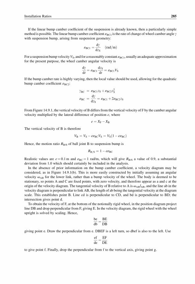
If the linear bump camber coefficient of the suspension is already known, then a particularly simple

method is possible. The linear bump camber coefficient «BC1 is the rate of change of wheel camber angle gwith suspension bump, arising from suspension geometry:

«BC1 ¼ dgdzS

ðrad=mÞ

For a suspension bumpvelocityVS, and for a reasonably constant «BC1, usually an adequate approximation

for the present purpose, the wheel camber angular velocity is

dgdt

¼ «BC1dzS

dt¼ «BC1VS

If the bump camber rate is highly varying, then the local value should be used, allowing for the quadratic

bump camber coefficient «BC2:

gBC ¼ «BC1zS þ «BC2z2S

«BC ¼ dgdzS

¼ «BC1 þ 2«BC2zS

From Figure 14.9.1, the vertical velocity of B differs from the vertical velocity of F by the camber angular

velocity multiplied by the lateral difference of position e, where

e ¼ XF �XB

The vertical velocity of B is therefore

VB ¼ VS � e«BCVS ¼ VSð1� e«BCÞ

Hence, the motion ratio RB/S of ball joint B to suspension bump is

RB=S ¼ 1� e«BC

Realistic values are e¼ 0.1m and «BC¼ 1 rad/m, which will give RB/S a value of 0.9, a substantial

deviation from 1.0 which should certainly be included in the analysis.

In the absence of prior information on the bump camber coefficient, a velocity diagram may be

considered, as in Figure 14.9.1(b). This is more easily constructed by initially assuming an angular

velocity vAB for the lower link, rather than a bump velocity of the wheel. The body is deemed to be

stationary, so points A and C are fixed points, with zero velocity, and therefore appear as a and c at the

origin of the velocity diagram. The tangential velocity of B relative to A is vABlAB, and the line ab in the

velocity diagram is perpendicular to link AB, the length of ab being the tangential velocity at the diagram

scale. This establishes point B. Line cd is perpendicular to CD, and bd is perpendicular to BD; the

intersection gives point d.

To obtain the velocity of F, at the bottom of the notionally rigid wheel, in the position diagram project

line DB and drop perpendicular from F, giving E. In the velocity diagram, the rigid wheel with the wheel

upright is solved by scaling. Hence,

be

db¼ BE

DB

giving point e. Draw the perpendicular from e. DBEF is a left turn, so dbef is also to the left. Use

ef

de¼ EF

DE

to give point f. Finally, drop the perpendicular from f to the vertical axis, giving point g.


This completes the velocity diagram to some convenient scale for some angular velocity vAB of the

lower arm. This methodology may, of course, form the basis of a computer program where repeated

analysis is desired.

The velocities of interest may now be read from the diagram:

(1) Thevertical velocity of the point F, that is, the suspension bump velocity,VS, is represented by

ag (VS¼VG/A).

(2) The wheel scrub (lateral) velocity VWS is represented by fg.

(3) The tangential velocity of D relative to B, VD/B, is represented by bd.

(4) The tangential velocity of D relative to C, VD/C, is represented by cd.

Hence the following may be deduced:

(1) The motion ratio of the lower arm to suspension bump, in units rad s�1/m s�1¼ rad/m, is

R ¼ vAB

VS

¼ VB=A

lABVS

(2) The camber angular velocity

dgdt

¼ VD=B

lDB

(3) The bump camber coefficient

«BC ¼ 1

VS

dgdt

¼ VD=B

lDBVS

¼ � ldb

lDBlag

(4) The basic roll centre height (unrolled)

hRC ¼ 1

2Tlfg

lag

In the present context, it is the velocity ratio that is of interest. The lower arm may then be analysed as a

rocker output for the spring or damper drive, as was the rigid arm, to give the overall motion ratio.

14.10 Struts

The strut suspension is the usual choice nowadays for the front of passenger cars. The use of a strut at the

rear is a little unusual, but has featured in several cases.

The usual strut incorporates the damper into the body of the strut, and has a surrounding spring. An

alternative design, the damper strut, has only the damper in the strut body,with the spring acting separately

on one of the arms. Geometrical considerations are the same, although, of course, in the latter case it is the

arm which must be analysed for the spring motion ratio.

Overall, the method of analysis is similar to that of the double-wishbone suspension. Figure 14.10.1(a)

shows a strut suspension. This is in fact the simpler version where the strut axis passes through the ball

joint at B.

If the bump camber coefficient is already available, then the vertical velocity VZB of B is given by

VZB ¼ VSð1� e«BCÞ


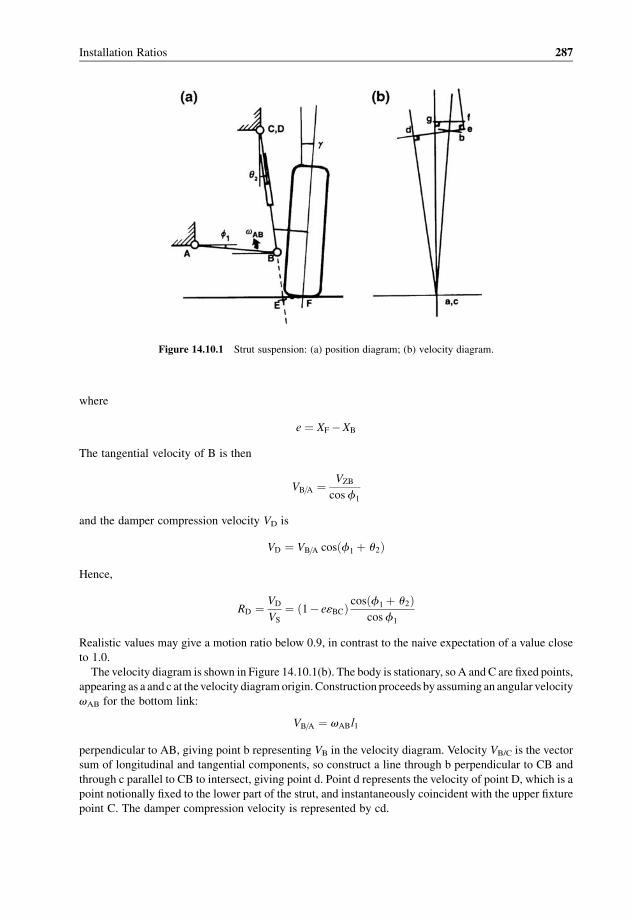
where

e ¼ XF �XB

The tangential velocity of B is then

VB=A ¼ VZB

cos f1

and the damper compression velocity VD is

VD ¼ VB=A cosðf1 þ u2Þ

Hence,

RD ¼ VD

VS

¼ ð1� e«BCÞ cosðf1 þ u2Þcosf1

Realistic values may give a motion ratio below 0.9, in contrast to the naive expectation of a value close

to 1.0.

The velocity diagram is shown in Figure 14.10.1(b). The body is stationary, so A and C are fixed points,

appearing as a and c at thevelocity diagramorigin. Construction proceeds by assuming an angular velocity

vAB for the bottom link:

VB=A ¼ vABl1

perpendicular to AB, giving point b representing VB in the velocity diagram. Velocity VB/C is the vector

sum of longitudinal and tangential components, so construct a line through b perpendicular to CB and

through c parallel to CB to intersect, giving point d. Point d represents the velocity of point D, which is a

point notionally fixed to the lower part of the strut, and instantaneously coincident with the upper fixture

point C. The damper compression velocity is represented by cd.

Figure 14.10.1 Strut suspension: (a) position diagram; (b) velocity diagram.


To obtain the suspension bump velocity, extend DB and drop the perpendicular from F to E. Use

be

bd¼ BE

BD;

ef

de¼ EF

DE

to give e and f, and drop the perpendicular from f onto the vertical axis to give g. Point f represents the

motion of the base of the wheel, and g represents its vertical component.

From the velocity diagram can be obtained:

(1) the suspension bump velocity represented by ag;

(2) the wheel scrub velocity (fg);

(3) the tangential velocity of B relative to D (db).

Hence, the following may be calculated:

(1) the motion ratio R of the lower arm to suspension bump

R ¼ vAB

VS

¼ VA=B

lAB VA=G

(2) the camber angular velocity

dgdt

¼ VB=D

lBD

(3) the bump camber coefficient

«BC ¼ dg=dtVS

¼ VB=D

lBD VS

¼ � lbd

lBD lagrad s--1=m s--1� �

(4) the basic roll centre height (unrolled)

hRC ¼ 1

2Tlfg

lag

On front suspensions in particular, the damper axis is frequently aligned such that it does not pass

through the ball joint at B, but rather inside or outside it. In that case the preceding analysis is still

applicable, with the following provisos:

(1) The angle u2 used is that of the damper axis, not that of the steering axis CB.

(2) To obtain e and f, still use the steering axis line CB extended.

14.11 Pushrods and Pullrods

In formula racing cars in particular, it is normal practice nowadays to use doublewishboneswith a pushrod

driving a rocker which operates the spring and damper. These can be solved readily by the processes

already described, treating the motion ratio as the product of the sequence of ratios arising from the

particular system. This generally involves:

(1) the relationship of wheel displacement to bottom arm angle;

(2) the relationship of bottom arm angle to pushrod displacement;

(3) the rocker ratio.


For a practical racing suspension, thewishbones are long and the pushrod anglemay be quite low, giving

a low velocity ratio. This gives proportionally larger pushrod forces, but the reduced stroke allows a

compact rocker. Pullrods have been used in the past, but have now largely given way to pushrods. The

pullrod analysis is very similar to that of the pushrod.

The rocker axis may be rotated to lay the damper along the vehicle.With the pushrod system this allows

the front dampers to lie above the driver’s legs, permitting the best aerodynamic shape for the front part of

the vehicle.

In these more complex systems, when analysed as a series of two-dimensional sub-mechanisms, it may

be necessary to incorporate some cosine factors to correct for out-of-plane motions, but these are usually

quite small.

14.12 Solid Axles

Solid car axles, driven or undriven, may be located either by leaf springs, the Hotchkiss axle if driven

(‘live’), or, more often nowadays, by links. The springs and dampers may act on the axle itself, or on the

links, as in Figure 14.12.1.

For bumpanalysis, if the spring or damper acts directly on the axle, as in Figure 14.12.2, above thewheel

centreline, and the springs or dampers are vertical, then the motion ratio is very close to 1.0. However, the

springs or dampers are sometimes angled, inwards at the top, inwhich case the bumpmotion ratio is cos uKor cos uD.If the springs act on the locating links, then the velocity diagram needs to be drawn, as in Figure 14.12.1.

With this configuration, some rising rate can be achieved by angling the springs or dampers in side view.

The vertical wheel velocity is found from thewheel centre, and its relationship to points B and C. The axle

angular speed vA is

vA ¼ VB=C

lBC

Figure 14.12.1 Example axle with link location, using a Watt’s linkage at each end.


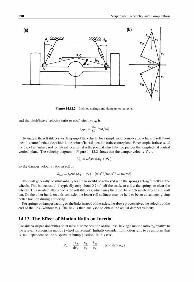
and the pitch/heave velocity ratio or coefficient «APH is

«APH ¼ vA

VS

rad=m½ �

Toanalyse the roll stiffness or dampingof thevehicle, for a simple axle, consider thevehicle to roll about

the rollcentre for theaxle,which is thepointof lateral location in thecentreplane.Forexample, in thecaseof

the use of a Panhard rod for lateral location, it is the point at which the rod pierces the longitudinal central

vertical plane. The velocity diagram in Figure 14.12.2 shows that the damper velocity VD is

VD ¼ vl1cosðf1 þ uKÞso the damper velocity ratio in roll is

RKf ¼ l1cos ðf1 þ uKÞ ½m s--1=rad s--1 ¼ m=rad�This will generally be substantially less than would be achieved with the springs acting directly at the

wheels. This is because l1 is typically only about 0.7 of half the track, to allow the springs to clear the

wheels. This substantially reduces the roll stiffness, which may therefore be supplemented by an anti-roll

bar. On the other hand, on a driven axle, the lower roll stiffness may be held to be an advantage, giving

better traction during cornering.

For springs or dampers acting on the links instead of the axles, the above process gives thevelocity of the

end of the link (without uK). The link is then analysed to obtain the actual damper velocity.

14.13 The Effect of Motion Ratio on Inertia

Consider a suspension with a point mass at some position on the links, having amotion ratioRm relative to

the relevant suspension motion (wheel movement). Initially consider this motion ratio to be uniform, that

is, not dependent on the suspension bump position. In this case,

Rm ¼ dxm

dzS¼ xm

zS¼ _xm

_zSðconstant RmÞ

Figure 14.12.2 Inclined springs and dampers on an axle.


where the movement of the mass is denoted by xm. This is not intended to suggest that the mass actually

moves in the x-coordinate direction, but to indicate that it is not generally in the same z-direction as the

suspension. The velocity of the mass is then

_xm ¼ Rm _zS ¼ RmVS

and the acceleration of the mass is

€xm ¼ Rm €zS ¼ RmAS

The force exerted on the mass to provide its acceleration is

Fm ¼ m €xm

Neglecting friction, the corresponding force FSm at the suspension point, by virtual work is given by

FSm dzS ¼ Fm dxm

giving

FSm ¼ dxm

dzSFm ¼ RmFm

This result also follows naturally from the concept of a frictionless lever. The force required at the

suspension is then

FSm ¼ RmFm ¼ Rmm €xm ¼ mR2m €zS

Therefore at a constant motion ratio the effective inertia, seen at the wheel, of a point mass, is just mR2m.

Although perhaps slightly laboured, this development shows the assumptions in the theory behind this

result.

The case of variable motion ratio is slightly more complicated. By definition, the motion ratio is, for

linear or non-linear cases,

Rm ¼ dxm

dzS¼ _xm

_zS

The time rate of variation of themotion ratio can usefully be expressed in terms of its spatial variation and

the suspension velocity:

_Rm ¼ dRm

dt¼ dRm

dzS� dzSdt

¼ R0m _zS

The velocity of the mass is simply

_xm ¼ Rm _zS

The acceleration of themass in terms of zS follows by the usual rules for differentiation of a product of two

variables:

€xm ¼ Rm €zS þ _Rm _zS

The force at the suspension is then

FSm ¼ RmFm ¼ Rmm €xm ¼ mRmðRm €zS þ _Rm _zSÞ


giving

FSm ¼ mðR2m €zS þRm

_Rm _zSÞSubstituting the result obtained earlier for the time derivative of Rm finally gives

FSm ¼ mðR2m €zS þRmR

0m _z

2SÞ

For a constantmotion ratio, this reduces to the earlier simple expression deduced for that case, as it should.

When the motion ratio is not constant, that is, actually varying with zS, then there is no simple equivalent

inertia.

14.14 The Effect of Motion Ratio on Springs

The spring stiffness depends on a spatial derivative of spring length, so the effect of the motion ratio of the

springs is in general different from the effect on inertia or damping coefficient. The spring may be linear

(constant stiffness) or non-linear, and themotion ratiomay be uniform in zS or non-uniform. It is generally

believed that the effect of motion ratio on effective spring stiffness as seen at the wheel is proportional to

the spring motion ratio squared. However, this is true only for a constant motion ratio.

Consider first a linear spring with constant motion ratio RK (recall that subscript K is used for springs

because subscript S has already been allocated to ‘suspension’). By definition, the motion ratio is

RK ¼ dxK

dzS¼ _xK

_zS

The spring force isFK and the spring stiffness isKK. By the principle of virtual work, or consideration of a

frictionless lever,

FK dxK ¼ FSK dzS

where FSK is the effective spring force seen at the active suspension point (wheel motion). This gives

FSK ¼ RKFK

The effective stiffness seen at the wheel, with constant RK, is

KSK ¼ dFSK

dzS¼ RK

dFK

dzS¼ RK

dFK

dxK

dxK

dzS¼ R2

KKK

So, for this simple case, the effective stiffness simply depends on R2K:

KSK ¼ R2KKK ðconstant RKÞ ð14:14:1Þ

Now consider a non-linear spring with a constant motion ratio:

KSK ¼ dFSK

dzS¼ dFSK

dxK� dxKdzS

¼ d

dxKðRKFKÞ � dxK

dzS

But the motion ratio RK is constant, so

KSK ¼ RK � dFK

dxK�RK ¼ R2

KKK


so the non-linearity of the spring does not alter the basic effective stiffness relationship, although, of

course, the local value of the spring stiffness must be used.

Consider now a linear spring with varying motion ratio, R0K 6¼ 0. The suspension force is as before:

FSK ¼ RKFK

where the local value of the motion ratio must be used, according to zS. By the usual differentiation of a

product,

KSK ¼ dFSK

dzS¼ d

dzSðRKFKÞ ¼ RK � dFK

dzSþ dRK

dzS�FK

The first term is as in equation (14.14.1), but there is now also a new term. The total stiffness is

KSK ¼ R2KKK þFK

dRK

dzSð14:14:2Þ

This additional second term is FKR0K. For the special case of constant RK the derivative vanishes and the

second term is zero, with equation (14.14.2) reducing to equation (14.14.1). The usual practical case is

with a derivative somewhat positive, that is, a ‘rising-rate’ suspension. With a large spring force FK, this

can have a considerable effect on the stiffness seen at the wheel. By way of example values, see

Table 14.14.1. In this example, the rising rate is only 2/m, about 0.05/inch, but the effect is substantial.

When a non-linear spring is used with a variable motion ratio, the theory is similar to the above. No

specific conclusions can be drawn, although equation (14.14.2) continues to apply.

Changing the motion ratio of the springs does not allow the use of reduced-mass springs. Of course, a

smaller motion ratio reduces the spring stroke required but correspondingly increases the force required

from it. These factors are simply in the ratio and inverse ratio respectively of themotion ratio, and have no

net effect. Also, by energy considerations, at least in the case of a linear spring it is fairly clear that an

intermediate lever does not reduce the mass required to store a given amount of energy, the work done in

bump action. This is confirmed by more detailed analysis.

14.15 The Effect of Motion Ratio on Dampers

It is generally believed that the effective damping coefficient is proportional to the damper motion ratio

squared. This is only true for a linear damper, andmay be seriously in error for non-linear cases as found on

many real dampers. However, a varying motion ratio is of no special significance for dampers, unlike

springs, only the local actual motion ratio value matters.

Table 14.14.1 Example values of rising-rate stiffness effect

Parameter Symbol Units Value

Suspension force FS kN 4.000

Motion ratio (ref) RK — 0.500

Spring force FK kN 8.000

Spring stiffness KK kN/m 128.0

Rising rate dRK/dzS m�1 2.000

Basic stiffness KKR2K kN/m 32.0

Rising rate stiffness FKR0K kN/m 16.0

Total stiffness KSK kN/m 48.0


Consider a linear damper with a constant motion ratio. It is evident that

FD¼CDVD

VD¼RDVS

FSD¼RDFD

FSD¼RDCDVD¼R2DCDVS

CSD¼R2DCD

so in this case the effective damping coefficient simply depends on the motion ratio squared.

Now consider a linear damper with a varying motion ratio,

FD¼CDVD

VD¼RDVS

FSD¼RDFD¼RDCDVD ¼ R2DCDVS

as before. Only the local value of the damper motion ratio RD affects the damper; unlike the case of a

spring, the gradient R0D has no effect.

Consider now a non-linear damper exerting a damper force FD related to the damper velocity VD by

FD ¼ C1VnD

where the exponent n has a value 1 for a linear damper (notionally pure viscosity), butmay vary in practice

from zero (effective Coulomb damping) to 2 (pure fluid dynamic damping). At a damper motion ratio RD

and suspension bump speed VS, the damper speed, positive in compression, is

VD ¼ RDVS

The actual damper force FD is

FD ¼ C1ðRDVSÞn

and the suspension damper force FSD at the wheel is

FSD ¼ RDFD

Hence the effective damping force at the wheel is

FSD ¼ C1R1þ nD Vn

S

The shape of the influence ofVS onFSD is retained as VnS , but the actual coefficient is scaled by the damper

coefficient ratio, which in this case is

RDC ¼ R1þ nD

Some special cases to be considered are the following:

(1) Exponent n¼ 0, corresponding to dry Coulomb friction (old-fashioned snubbers) or to hydraulic

dampers with a sudden-acting blow-off valve. In this case the damper velocity makes no difference,

as long as it is moving, so the coefficient ratio and the force ratio are both equal to the velocity

ratio:

RDC ¼ RD ðn ¼ 0Þ


(2) Exponent n¼ 1, corresponding to a linear damper:

RDC ¼ R2D ðn ¼ 1Þ

(3) Exponentn¼ 2, corresponding to a hydraulic damperwith a valve that is fixed, (e.g. fully closed at low

speed or fully open at high speed):

RDC ¼ R3D ðn ¼ 2Þ

(4) A representative intermediate case at damper speeds around the knee of the curve, with n� 0.5,

giving

RDC ¼ R1:5D ðn ¼ 0:5Þ

It is common for the motion ratio to be around 0.7, sometimes even as low as 0.4, from which it will

be apparent that the damper coefficient ratio will vary very widely for different damper force–speed

relationships.

Considered from a design aspect, the characteristic required at the wheel is the starting point, which is

transformed by the motion ratio to the required damper characteristic. A low motion ratio therefore calls

for a high damping coefficient for the damper itself. The use of a low or high motion ratio does not allow

the use of a smaller or lighter damper. A lowmotion ratio reduces the stroke required, but correspondingly

increases the damper force needed.

14.16 Velocity Diagrams in Three Dimensions

The three-dimensional velocity diagram is, in principle, a straightforward extension of the idea of the two-

dimensional velocity diagram, but in practice is a good deal more difficult conceptually. All velocities

have three components, e.g. VA¼ (VAx,VAy,VAz) for a point A, this velocity being ‘plotted’ in a three-

dimensional velocity space. Themethod used is in effect geometrical constructions in a three-dimensional

space. Actual drawing-instrument methods are not practical, although the results can be drawn as iso-

metrics, and the solution must be by algebraic methods. The solution can often use existing three-

dimensional geometry library routines. The alternative method of determining the velocities by a small

displacement using an existing suspension position solver is generally easier, although imperfect in

principle because of the increment size required for accuracy. The three-dimensional velocity diagramhas

the merit of being an exact method in principle.

In all cases, the position of the suspension must first be fully known. In the case of a double-transverse-

arm suspension, proceed by specifying an angular velocityV of the bottom arm. The tangential velocity of

the lower outer ball joint point A is thenVR, with a direction perpendicular to the plane of the lower arm.

The direction cosines (l, m, n) of the normal to the plane are therefore also the direction cosines of the

velocity direction, so the velocity components can be deduced, giving

V�A ¼ ðVAx;VAy;VAzÞ ¼ VAðl;m; nÞThe velocity of the upper outer ball joint B relative to the velocity point a for physical point A is just

tangential. Therefore it is in a plane through velocity point a, perpendicular to the line fromone ball joint to

the other. The direction cosines of the normal for this plane are therefore those of the line AB. This gives a

known plane in the velocity diagram through the knownvelocity point a. Also, the upper ball joint velocity

must be perpendicular to the plane of the upper arm, giving a line from the velocity origin parallel to the

normal to the plane. The intersection of the line and the plane in the velocity diagram gives point b, the

velocity of upper ball joint point B.

To complete the solution of the wheel carrier/slider, the velocity of the steering-arm/track-rod end ball

joint is required. Unlike in the case of two-dimensional velocity diagrams, in three dimensions a solid


component does not have a similar velocity image, and the image is distorted. The clearest method is to

drop a perpendicular from the steering-arm ball joint C onto the steer axis AB, giving a foot point F. Now a

straight line in an ideally-rigid object doesmap into a straight-line image in the three-dimensional velocity

diagram, so velocity point f can be calculated by simple proportion from velocity points a and b, in the

same ratio as F lies on AB or AB extended. The velocity of C relative to F is purely tangential, and is

therefore perpendicular to the planeABCF,which has a normalwith solvable direction cosines.Hence, the

direction cosines of the line fc can be found, giving a line fc, so far of unknown length, from the known

point f. Considering the rack end of the track rod, this pointDhas a known, specified velocity depending on

the rack only, usually zero, giving velocity point d. Relative to D, the track-rod end C has a velocity

perpendicular to the line CD, so it is in a plane in the velocity diagram perpendicular to line CD and

containing the origin. The line from f intersects this plane at velocity point c for physical point C,

completing the basic solution of the wheel upright. The three known velocities for points A, B and C can

nowbe used to calculate angular velocities about theX,Y andZ axes, that is, the bumpcamber, bump caster

and bump steer angular velocities.

To solve the scrub velocity at the contact point D, thewheel is treated as locked in rolling rotation, so the

wheel and wheel carrier are considered to be a single rigid component. The contact point D is therefore a

fixed point on the carrier. Drop a perpendicular fromD to a new foot E on the ball joint line AB produced,

solving e on ab by the same proportion as E onAB. Also, use the tangential velocity of C and the length of

FC to obtain an angular velocity of the carrier about the axis AB. Apply this to DE to obtain a relative

tangential velocity of D from E, which has the direction of the normal to the plane ABFED, hence solving

the magnitude and direction of the velocity of D. This resulting velocity

VD ¼ ðVDx;VDy;VDzÞ

contains the longitudinal scrub velocityVDx, the lateral scrub velocityVDy, and the bump velocityVDz. All

the bump coefficients then follow easily; for example, the local longitudinal bump scrub rate coefficient is

«BScd;X ¼ VDx

VDz

and the local lateral bump scrub rate coefficient is

«BScd;Y ¼ VDy

VDz

Obtaining values for these over a range of suspension bump positions, the usual coefficients may be

obtained, using

«BScd ¼ «BScd0 þ «BScd1zS

applied in longitudinal and transverse directions.

In principle, to find the suspension bumpvelocity, find thewheel centrevelocity, and deduce thevelocity

of the lowest point of the wheel arc, allowing wheel rotation, that is, the lowest point of a circle on the

wheel centre with radius equal to the wheel loaded radius. The wheel centre is a fixed point on the wheel

carrier. The velocity of the lowest point is the velocity of thewheel centre plus the change in height due to

camber change from wheel loaded radius, camber angle and camber angular velocity. Considering the

wheel as free to rotate allows the bottom point to have an extra motion giving a tangential velocity

component, which is purely horizontal. This leaves the lateral scrub component and the bump velocity

unchanged. The result is therefore the same as above – simply the vertical component of the locked-wheel

bottom point velocity, namely VDz.

For a strut-and-arm suspension, again begin with a bottom arm angular velocity and the bottom ball

joint point A. Obtain the velocity component directly towards the fixed trunnion point B. Point C on the


slider, instantaneously coincidentwithB, has a velocityVC directed along the slider, butwith a component

in the direction of AB equal to the component of VA in that direction. This is because for two points on a

rigid body the separation is constant, so the velocity components along the line of the pointsmust be equal.

Hence, vector dot products can be used to obtain VC. This gives the velocity of two known points of the

carrier/slider. The rack end D has a known, independently specified, velocity, probably zero. To solve for

the steering-arm/track-rod end E, at the track-rod end this has a velocity in a plane perpendicular to DE

from the velocity point d. Also, considering it as the steering-arm end, drop a perpendicular from E onto

the lineAC to footG, solving g by proportion. ThevelocityVE/G is perpendicular the planeACGE, giving a

line in the velocity diagram from g, intersecting the plane from d at the desired point e. Hence, the carrier/

slider has three known velocity points, and is solved. The velocity of the contact point can be solved as for

the double-transverse-arm suspension.

Other suspension types can be solved using similar methods. The use of three-dimensional geometrical

routines in the process of solution is apparent. In position analysis, the two main three-dimensional

procedures are the ‘pole-on-triangle’ and the ‘tripod’. Correspondingly, two main velocity diagram

procedures can be used, rather than the ad hoc approach above.

The ‘pole-on-triangle’ velocity diagram procedure is required to solve the velocity of a point fixed

relative to a base triangle which moves but is of unchanging shape and size. The first perpendicular

required is that fromP ‘down’ to F in the plane of the triangle. Point F has factors for its position relative to

the three corners of the triangle. The velocity of F is found by applying the same factors to the corner

velocities. Also drop the perpendicular from the point P1 into the line P2P3 of the triangle to give a foot P4.

The velocity of P4 may be found by proportion, using the interpolation factors of the physical point P4 on

P2P3. Next, calculate angular velocities about the rectangular axes aligned with P2P3 and P1P4. Use these

angular velocities to calculate thevelocity of P relative to thevelocity of F.Chapter 15 gives further details.

The ‘Tripod’ position problemhas an analogue in the tripod velocity problem, butwhereas the first is the

intersection of three spheres, the latter is the intersection of three planes in thevelocity diagram, associated

with three simultaneous linear equations. Consider rod 1, with base velocity (u1, v1,w1) and rod centreline

direction cosines (l1, m1, n1). In the velocity diagram, the known base velocity gives a point, and the

velocity of the other end of the rod must be in a plane through that point, the plane having a normal with

direction cosines the same as the rod. The equation of that plane is simply

l1uþm1vþ n1w ¼ l1u1 þm1v1 þ n1w1

There are three such equations, so the unknowns (u, v,w) can be solved, this being the intersection point of

the three planes. Tantalisingly, it is possible to solve explicitly using a direct line-and-planemethod, using

say rod 1 to give a plane, and rods 2 and 3 to give a line. This line is of course the intersection of thevelocity

planes of rods 2 and 3. The out-of-line velocities of the rod ends are independent because, instantaneously,

they do not act along the rods, they only rotate them about a transverse axis. Taking a pair of rods, the total

velocity of the joint point can be seen as one part perpendicular to the plane of the triangle, and one part in

the plane. The latter part can be solved from the in-plane base velocities by two-dimensional methods,

giving a velocity point. From there, the velocity of P is on a line perpendicular to the triangle, giving a line

to intersect the plane of rod 1. This is, however, actuallymore difficult to implement than the general three-

plane method.

14.17 Acceleration Diagrams

Acceleration diagrams are important in general mechanism design. In the case of vehicle suspensions,

there are two applications. The first is a determination of the accurate accelerations of the suspension

components to evaluate the acceleration forces. The second is for use as a derivative in the evaluation of

velocity diagrams.Acceleration diagrams are quite easy in twodimensions for simplemechanisms such as

pin-jointed ones (e.g. wishbones), and somewhat trickier for struts. In three dimensions they can become

very tricky.


References

Morrison, J.L.M. and Crossland, B. (1970) An Introduction to the Mechanics of Machines, 2nd edn in SI units,

London: Longman. ISBN 0582447291 and 0582447313. Contains material on velocity and acceleration diagrams.

Open University Course T235, Engineering Mechanics: Solids, contains detailed material on drawing velocity

diagrams. The entire course (on basic mechanical engineering) is available free at http://intranet.open.ac.uk/

open-content/. Click on ‘Visit the OpenLearn website’, enter ‘LabSpace’, click on topics ‘Technology’, scroll down

to ‘Engineering Mechanics: Solids’ and click on ‘Browse’. See Block 3 for velocity diagrams.

————— // —————


15

Computational Geometryin Three Dimensions

15.1 Introduction

The numerical or computational solution of a suspension geometry problem depends heavily on three-

dimensional coordinate geometry, which just is a more complicated variant of the more familiar two-

dimensional flat-plane paper-surface geometry. It is assumed here that the reader is familiar with basic

two-dimensional coordinate geometry and has studied basic three-dimensional geometry and vector

analysis. Presented here is an aide-m�emoire of some useful reference material, and the mathematical

solution of some problems particularly relevant to the solution of suspension geometry.

Although it seems physically that a point is simpler than a linewhich is simpler than a surface, this belies

the problems of mathematical representation. A surface can be represented by a single equation. It takes

two equations to represent a line (the intersection of two surfaces) and three equations to represent a point

(the intersection of three surfaces). In fact, it is oftenmost convenient to represent a line by three equations,

in its parametric form.

In general, algebraic variables are in italic, to indicate that they represent a value. Vectors are indicated

by bold type, but they are still variables so they are in bold italic. The point named P1, in non-bold roman

(upright) script has a position vector P1 in bold italic, which has a magnitude P1, which is non-bold italic.

15.2 Coordinate Systems

Overwhelmingly, the coordinate system of greatest importance and use is the one of simple rectangular

axes, typified by the usual (X, Y, Z) system.However, cylindrical coordinates are sometimes used, in effect

just polar coordinates plus a length dimension. This can arise, for example, in the case of a suspension arm,

which rotates about an axis at some arbitrary angle. The motion of the outer end of the arm is an arc which

is not conveniently represented in the coordinate system of the vehicle body, but using cylindrical

coordinates aligned with the axis the movement becomes simply a circular motion.

Sometimes linear non-rectangular coordinates can be used advantageously, as in the case of the PointIT

routine (Section 15.17).

The distance between two points is given by Pythagoras’ theorem in three dimensions, in rectangular

coordinates, by

LAB ¼ffiffiffiffiffiffiffiffiffiffiffiffiffiffiffiffiffiffiffiffiffiffiffiffiffiffiffiffiffiffiffiffiffiffiffiffiffiffiffiffiffiffiffiffiffiffiffiffiffiffiffiffiffiffiffiffiffiffiffiffiffiffiffiffiffiffiffiffiffiffiffiffiffiðxA � xBÞ2 þðyA � yBÞ2 þðzA � zBÞ2

q


This is invariably a positive number, possibly zero. The squares inside the root ensure that the kernel can

never be negative.

The idea of a length, which is never negative, must be distinguished carefully from the idea of a

displacement or position,whichmay be negative. In a coordinate system, thevariables represent positions,

not lengths, and can be negative, indicating a location in the other direction. This distinction between

length and displacement also arises importantly in the case of the position of a point ‘above’ a plane. Given

a specific plane normal, the point displacement from the plane could be positive ‘up’ or negative ‘down’,

for example as in the PointAT routine (Sections 15.21 and 15.22).

15.3 Transformation of Coordinates

It is often convenient to retain rectangular coordinates but to shift the origin. Thismay be done to facilitate

algebraic solution of problems, or to improve computational efficiency. Considering base coordinates

(x, y, z), and local coordinates (u, v,w) which are parallel to (x, y, z) but displacedwithout rotation, placing

the origin of (u, v, w) at P1¼ (x1, y1, z1) gives

u1 ¼ 0; v1 ¼ 0; w1 ¼ 0

u2 ¼ x2 � x1; v2 ¼ y2 � y1; w2 ¼ z2 � z1

and so on.

Rotation of coordinates is less often required, but is easily achieved. In the base coordinates (x, y, z) the

alternative coordinate system (u, v,w) has the same origin and is rotated such that the direction cosines of

(u, v, w) in (x, y, z) are (lu, mu, nu), (lv, mv, nv) and (lw, mw, nw), giving the transformation

u ¼ lux þ muy þ nuz

v ¼ lvx þ mvy þ nvz

w ¼ lwx þ mwy þ nwz

The direction cosines of the secondary axes are not fully independent (nine direction cosines but only three

degrees of freedom), and compatibility must be maintained.

If the origin is simultaneously moved to (x0, y0, z0) then the combined transformation is

u ¼ luðx� x0Þ þ muðy� y0Þ þ nuðz� z0Þv ¼ lvðx� x0Þ þ mvðy� y0Þ þ nvðz� z0Þw ¼ lwðx� x0Þ þ mwðy� y0Þ þ nwðz� z0Þ

15.4 Direction Numbers and Cosines

Consider a straight line with any two distinct points upon it. By Pythagoras’ theorem the length is

L12 ¼ffiffiffiffiffiffiffiffiffiffiffiffiffiffiffiffiffiffiffiffiffiffiffiffiffiffiffiffiffiffiffiffiffiffiffiffiffiffiffiffiffiffiffiffiffiffiffiffiffiffiffiffiffiffiffiffiffiffiffiffiffiffiffiffiffiffiffiffiffiffiffiðx2 � x1Þ2 þ ðy2 � y1Þ2 þ ðz2 � z1Þ2

q

In rectangular coordinates, any set of three numbers, usually denoted (L, M, N), being

ðL;M;NÞ ¼ ððx2 � x1Þ; ðy2 � y1Þ; ðz2 � z1ÞÞ

is called a set of the direction numbers for the line. Points P1 and P2 and the length L12 may vary, only the

ratios of the direction numbers are significant. The direction numbers are sometimes also known as

direction ratios, but this is not a good name as individually they are displacements.


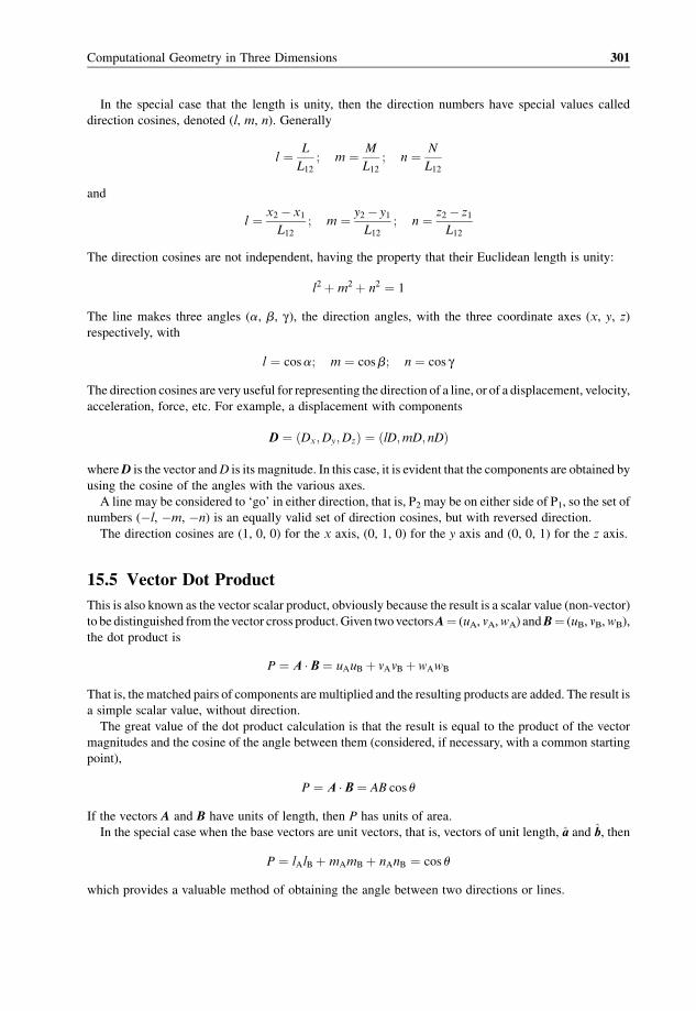
In the special case that the length is unity, then the direction numbers have special values called

direction cosines, denoted (l, m, n). Generally

l ¼ L

L12; m ¼ M

L12; n ¼ N

L12

and

l ¼ x2 � x1

L12; m ¼ y2 � y1

L12; n ¼ z2 � z1

L12

The direction cosines are not independent, having the property that their Euclidean length is unity:

l2 þ m2 þ n2 ¼ 1

The line makes three angles (a, b, g), the direction angles, with the three coordinate axes (x, y, z)

respectively, with

l ¼ cosa; m ¼ cosb; n ¼ cos g

The direction cosines are very useful for representing the direction of a line, or of a displacement, velocity,

acceleration, force, etc. For example, a displacement with components

D ¼ ðDx;Dy;DzÞ ¼ ðlD;mD; nDÞ

whereD is the vector andD is its magnitude. In this case, it is evident that the components are obtained by

using the cosine of the angles with the various axes.

A line may be considered to ‘go’ in either direction, that is, P2 may be on either side of P1, so the set of

numbers (�l, �m, �n) is an equally valid set of direction cosines, but with reversed direction.

The direction cosines are (1, 0, 0) for the x axis, (0, 1, 0) for the y axis and (0, 0, 1) for the z axis.

15.5 Vector Dot Product

This is also known as the vector scalar product, obviously because the result is a scalar value (non-vector)

to be distinguished from thevector cross product.Given twovectorsA¼ (uA, vA,wA) andB¼ (uB, vB,wB),

the dot product is

P ¼ A �B ¼ uAuB þ vAvB þwAwB

That is, thematched pairs of components are multiplied and the resulting products are added. The result is

a simple scalar value, without direction.

The great value of the dot product calculation is that the result is equal to the product of the vector

magnitudes and the cosine of the angle between them (considered, if necessary, with a common starting

point),

P ¼ A �B ¼ AB cos u

If the vectors A and B have units of length, then P has units of area.

In the special case when the base vectors are unit vectors, that is, vectors of unit length, a and b, then

P ¼ lAlB þ mAmB þ nAnB ¼ cos u

which provides a valuable method of obtaining the angle between two directions or lines.

Computational Geometry in Three Dimensions 301

In the event that the angle is a right angle (90�), then the cosine and the dot product must be zero, which

can be a useful check on the perpendicularity of two lines.

A key application of the dot product is in obtaining components of displacements, velocities,

accelerations, forces, etc., along any direction. Given a vector A with components (xA, yA, zA) and a

line with direction cosines (l, m, n), then the component of A in that direction is

Acomp ¼ lxA þ myA þ nzA

If the other direction of the line is considered, then all three direction cosines are reversed in sign, and

the component changes sign but retains its magnitude.

Consider, for example, a moving rigid rod AB, with velocities at its ends

VA ¼ ðuA; vA;wAÞVB ¼ ðuB; vB;wBÞ

The rod end positions are (xA, yA, zA) and (xB, yB, zB). Then the direction cosines of the rod, A to B, are

l ¼ xB � xA

LAB; m ¼ yB � yA

LAB; n ¼ zB � zA

LAB

The velocity component at A in the direction of the rod itself, that is, the axial velocity of the rod, is, by the

dot product,

VA;axial ¼ luA þ mvA þ nwA

Similarly, at the other end,

VB;axial ¼ luB þ mvB þ nwB

For a rigid rod, these two axial components must be equal.

A good example application of the dot product may be found in Section 15.14.

15.6 Vector Cross Product

The vector cross product, denoted

P ¼ A� B

is itself a vector, with magnitude

P ¼ AB sin u

where the angle u is the angle between the two vectors, considered if necessary to be translated to a

common starting point. IfA andB have units of length, then P has units of area, and is in fact the area of a

parallelogramdefined by the twovectors, that is, twice the area of the triangle that they form. The direction

of the resulting vector is perpendicular to bothA andB, being given by the right-hand rule.WhereA is the

right-hand thumb, andB is the first finger, thenP is in the direction of the secondfinger. IfA andB are taken

in the other order, then the product is reversed in direction, that is,

B� A ¼ �A� B

The product vector A�B has the property that it is parallel to the normal to the plane containing the

vectors A and B. This is probably its most important feature, as it can therefore be used to generate that

normal vector.


The actual calculation can conveniently be summarised in a determinant. A generally non-unit vectorNwith the normal direction to the plane of A and B is given by the easily remembered form

N ¼ A� B ¼i j kxA yA zAxB yB zB

��

where (i; j; k) with circumflex marks are unit vectors of the (x, y, z) axes respectively. Expanding the

determinant in the usual way, with alternating signs,

N ¼ iðyAzB � yBzAÞ� jðxAzB � xBzAÞþ kðxAyB � xByAÞ¼ iNx þ jNy þ kNz

This calculation of the vector normal to a plane is frequently required in suspension geometry analysis.

15.7 The Sine Rule

The sine rule is occasionally useful in suspension analysis, and applies to three-dimensional triangles as

well as to two-dimensional ones, both being of necessity in a single plane, Figure 15.7.1. However, it is

expressed in terms of the two-dimensional properties of the triangle rather than in direct three-dimensional

terms. For a triangle with sides a, b and c, with opposing angles A, B and C,

sin A

a¼ sin B

b¼ sin C

c

It is easily proved by dropping a perpendicular. It can equally well be expressed in reciprocal form,

a/sinA¼ b/sinB¼ c/sinC.

In three dimensions, considering the cross product of various pairs of sides, in each case the magnitude

of the product is equal to twice the area of the triangle. Hence,

L31L12 sin u1 ¼ L12L23 sin u2 ¼ L23L31 sin u3 ¼ 2ST

Dividing by L12L23L31 gives

sin u1L23

¼ sin u2L31

¼ sin u3L12

agreeing with the sine rule as expressed in two-dimensional terms.

Figure 15.7.1 Triangles for the sine rule, alternative notations.


15.8 The Cosine Rule

The cosine rule is often useful, much more so than the sine rule. In Figure 15.8.1, the three sides of any

planar triangle are related by

a2 ¼ b2 þ c2 � 2bc cos A

or

cos A ¼ b2 þ c2 � a2

2bc

In three-dimensional terms, the cosine ofA is given by the dot product, in local coordinates based on P1, as

ðP2 �P1Þ � ðP3 �P1Þ ¼ bc cos A

with

cos A ¼ u2u3 þ v2v3 þ w2w3

L31L12

Actually,

b2 þ c2 � a2 ¼ ðu22 þ v22 þw22Þþ ðu23 þ v23 þw2

3Þ� ðu3 � u2Þ2 �ðv3 � v2Þ2 �ðw3 �w2Þ2

¼ 2ðu2u3 þ v2v3 þw2w3Þ¼ 2ðP2 �P1Þ � ðP3 �P1Þ¼ 2bc cos A

That is,

cos A ¼ b2 þ c2 � a

2bc

proving the cosine rule directly in three-dimensional coordinates.

The component b cos A is sometimes useful, being given by

b cos A ¼ b2 þ c2 � a2

2c

without use of the (computationally relatively slow) transcendental cosine function.

Figure 15.8.1 Triangles for the cosine rule, alternative notations.


15.9 Points

In geometry, a point is an ideal concept of location, with zero extension is space, being just a position. It is

often defined as the intersection of two ideal geometric lines having no thickness, but this is applicable

only in two dimensions. In three dimensions two lines do not meet, in general. The point could then be

defined as the intersection of three planes, or of a linewith a plane, or of a linewith some other surface such

as a spherical shell or a cone.

In practical three-dimensional coordinate geometry the point, having three degrees of freedom, is a

position in space measured by three coordinates. These are the coordinates of the system in use, usually a

rectangular coordinate system, so the point becomes the location (x, y, z). However, a point on a line is

constrained in two degrees of freedom, and may be represented by a single parameter, for example the

parameter of path length s in the parametric representation of a line.

15.10 Lines

The geometric definition of a point as the intersection of two lines (in two dimensions) may be regarded

as somewhat circular, as a line is often defined as passing through two points, that is, two distinct

points are sufficient to define a straight line. This is still true in three dimensions. A straight line can also

be considered to be the intersection of two planes. In general, the intersection of two surfaces gives

a line, not necessarily straight, for example a plane and a spherical shell gives a circle, and in some

cases the line may be in distinct parts, as in the case of the intersection of a plane with a torus in some

positions.

In the main, however, it is the straight line and circle that are of importance. There are several common

and useful alternative forms of representation of a straight line.

(1) The standard form of a line between two points P1 and P2:

x� x1

x2 � x1¼ y� y1

y2 � y1¼ z� z1

z2 � z1

(2) The standard form of a line through P1 with direction cosines (l, m, n):

x� x1

l¼ y� y1

m¼ z� z1

n

This is also correct when direction numbers (L,M,N) are used instead, as these are in the same ratio to

each other:

x� x1

L¼ y� y1

M¼ z� z1

N

which is equivalent to the standard form.

(3) The parametric form of a line between two points:

x ¼ x1 þ f ðx2 � x1Þy ¼ y1 þ f ðy2 � y1Þz ¼ z1 þ f ðz2 � z1Þ

Here, the value of the parameter f controls the position of a point on the line. At P1 we have f¼ 0,

whereas at P2we have f¼ 1. Thevalue of fmay also be negative, with the point on P2 to P1 extended, or

greater than 1 with the point on P1 to P2 extended. Calculating a length L12 for P1 to P2, it is apparent


that the displacement of the point from P1 is

s ¼ f L12

(4) The parametric form of a line with known direction cosines. This is a special case of the above in

which a point P2 is considered to be unit distance from P1, that is, L12¼ 1. The parameter f then

becomes the actual path length from P1, so, for example,

x ¼ x1 þ sx2 � x1

L12¼ x1 þ sl

where l is the direction cosine, giving in all

x ¼ x1 þ l s

y ¼ y1 þ m s

z ¼ z1 þ n s

This parametric form is the most convenient form for general use.

15.11 Planes

The plane can be expressed in a single equation, but in various alternative ways.

(1) The general form is given by

Ax þ By þ Cz þ D ¼ 0

Here (A,B,C) are called the direction numbers, and are actually direction numbers of the normal to the

plane. In the general form, the constant D is included in the left-hand side.

(2) The normal form is

lx þ my þ nz ¼ p

Here (l,m, n) are the direction cosines of the normal to the plane. The variable p is the signed length of

the normal from the origin to the plane in the direction (l, m, n). Note that, in contrast to the general

form, p appears on the right-hand side of the equation. This normal form is the most useful form

overall.

(3) The intercept form is written as

x

aþ y

bþ z

c¼ 1

Thevariables a, b and c are the intercepts of the plane on thex, y and z axes, respectively. In suspension

analysis, this is not a very useful form. By multiplying the intercept form shown by abc the general

form may easily be obtained.

(4) The final way is as a plane through three points. A plane passing through three points P1, P2 and P3having coordinates (x1, y1, z1) et cetera has the equation given by the determinant

x� x1 y� y1 z� z1

x2 � x1 y2 � y1 z2 � z1

x3 � x1 y3 � y1 z3 � z1

��

��¼ 0


This form evidently gives preference to the point P1, which is treated somewhat as an origin of local

coordinates, and two alternative forms could be written based on the other two points. In local coordinate

variables based on P1 the above determinant becomes particularly simple:

u v w

u2 v2 w2

u3 v3 w3

�� ¼ 0

Expanding the determinant gives:

uðv2w3 � v3w2Þ� vðu2w3 � u3w2Þþwðu2v3 � u3v2Þ ¼ 0

Comparing this with the normal form

lx þ my þ nz ¼ p

it is apparent that the length of the perpendicular from the origin to the plane is zero. This is correct in local

coordinates based on P1, which is a point at the origin and in the plane. The direction numbers of the plane

are evidently

L ¼ v2w3 � v3w2

M ¼ u3w2 � u2w3

N ¼ u2v3 � u3v2

This is the same result as would be obtained by taking the vector cross product of (P2�P1) and (P3�P1)

in that order, giving a vector normal to the plane. This vector can then be divided by its length to give

direction cosines for the normal.

15.12 Spheres

Spheres, or perhaps more correctly geometric spherical shells, often arise in suspension analysis. Their

representation is simple, but not always convenient for analysis because the equation is non-linear. For a

radius R1 on a centre point (x1, y1, z1), the distance from the centre point, as simply given by Pythagoras’

equation in three dimensions, is constant, giving

x� x1ð Þ2 þ y� y1ð Þ2 þ z� z1ð Þ2 ¼ R21

This expands to

x2 þ y2 þ z2 � 2x1x� 2y1y� 2z1z ¼ R21 �ðx21 þ y21 þ z21Þ

where the right-hand side is constant.

The intersection of two spheres is an important practical problem. Where the intersection does occur,

the result is generally a circle, although a single touching point is a possibility in principle. Subtracting the

equations of two spheres gives the equation of a plane. This is called the radical plane of the two spheres.

It is perpendicular to the line joining the centres, that is to say, the line of the centres is its normal. If the two

spheres do not intersect, then the radical plane lies between the spheres. If they do intersect, then the circle

of intersection lies in the radical plane. Considering two spheres with equations as above, that is,

x2 þ y2 þ z2 � 2x1x� 2y1y� 2z1z ¼ c1

x2 þ y2 þ z2 � 2x2x� 2y2y� 2z2z ¼ c2


subtraction gives the equation of the radical plane as

ðx2 � x1Þx þ ðy2 � y1Þy þ ðz2 � z1Þz ¼ c1 � c2

2

Dividing this by the length L12 between the centres immediately gives the normal form of a plane. The

direction cosines are evidently directed along the line of the centres, so the plane itself is perpendicular to

that line, as would be expected by symmetry.

15.13 Circles

In two-dimensional geometry, circles are easily represented and, although non-linear, are highly analytic.

In three dimensions, the circle can be inconvenient to represent because it may be at any orientation.

The circle is a line, so being the intersection of two surfaces, and requiring two simultaneous equations.

One combination is the plane of the circle with the centre and a given radius. In effect, then, the circle is

represented as the intersection of a plane with a sphere, giving a great circle of the sphere. In some cases,

the circle arises naturally as the intersection of two spheres, probably of unequal radius, as in the case of a

suspension arm producing the circular arc of the outer ball joint.

To represent the circle in this waywe can use seven variables: the circle centre (xC, yC, zC), the direction

cosines of the normal to the plane of the circle (l,m, n) and the radius R. A point has only three degrees of

freedom, so evidently these seven variables contain some redundancy. Actually it is not necessary to

specify the centre, it may be convenient to specify any point on the axis, along with one point of the circle,

(xA, yA, zA, l,m, n, x1, y1, z1), using nine variables. The circle is then perceived as a section of a circular

cylinder.

To actually deal with the circle numerically, it is really necessary to use local coordinates with the

correct alignment. It is most convenient to have one given point on the circle itself (which, in practice, is

usually available) along with the axis, if necessary dropping a perpendicular to establish the centre of the

circle. The local coordinates (u, v, w) then have an origin at the centre of the circle (xC,yC,zC). The third

axisw points along the axis (l,m, n). The first axis u points from the centre towards the known point of the

circle. Considering unit vectors u and w in these directions, the unit vector

v ¼ w� u

from the cross product gives the desired third axis, perpendicular to the other two, with ðu; v; wÞ being aright-hand set. In more detail

v ¼ w� u ¼i j klw mw nwlu mu nu

��

so

lv ¼ mwnu �munw

mv ¼ lunw � lwnu

nv ¼ lwmu � lumw

A rotation of the arm or radius by angle u from the first position, right-hand about w then gives a local

coordinate position

u ¼ R cos u

v ¼ R sin u

w ¼ 0


This position can then be converted into (x, y, z) coordinates as described in Section 15.3. In calculation of

the last axis v by the vector cross product, the correct order of the vectors must be maintained to give a

right-hand set of conventional notation.

15.14 Routine PointFPL2P

Purpose: ‘Point at Foot of Perpendicular onto Line of 2 Points’ – to obtain the point F at the foot of a

perpendicular dropped from a specified point P onto a line defined by two points

Inputs: Coordinates of line points P1 and P2, and of point P, i.e. coordinates (x1, y1, z1), (x2, y2, z2),

(xP, yP, zP)

Outputs: The foot point coordinates (xF, yF, zF), and the perpendicular length LPF

Notes: None

Solution: The required point lies at some fraction f from P1 towards P2 (where the fraction f may also be

negative or exceed 1). This point has

x ¼ x1þ f ðx2�x1Þ ¼ ð1� f Þx1þ fx2

y ¼ y1 þ f ðy2 � y1Þ ¼ ð1� f Þy1 þ fy2

z ¼ z1 þ f ðz2 � z1Þ ¼ ð1� f Þz1 þ fz2

ð15:14:1Þ

The line from P to (x, y, z) must be perpendicular to the line P1P2. Therefore the dot product (equal to

cos u) must be zero, requiring

ðxF � xPÞðx2 � x1Þþ ðyF � yPÞðy2 � y1Þþ ðzF � zPÞðz2 � z1Þ ¼ 0

By substitution, an equation is obtained for the fraction f:

ðx1 þ f ðx2 � x1ÞÞðx2 � x1Þþ ðy1 þ f ðy2 � y1ÞÞðy2 � y1Þþ ðz1 þ f ðz2 � z1ÞÞðz2 � z1Þ ¼ 0

x1ðx2 � x1Þþ f ðx2 � x1Þ2 þ y1ðy2 � y1Þþ f ðy2 � y1Þ2 þ z1ðz2 � z1Þþ f ðz2 � z1Þ2 ¼ 0

with the result

f ¼ ðx1x2 þ y1y2 þ z1z2Þ� ðx21 þ y21 þ z21ÞL212

Substituting the value of f back into equations (15.14.1) gives the desired coordinates of the foot F.

Also, the length of the perpendicular is

LPF ¼ffiffiffiffiffiffiffiffiffiffiffiffiffiffiffiffiffiffiffiffiffiffiffiffiffiffiffiffiffiffiffiffiffiffiffiffiffiffiffiffiffiffiffiffiffiffiffiffiffiffiffiffiffiffiffiffiffiffiffiffiffiffiffiffiffiffiffiffiffiffiðxF � xPÞ2 þðyF � yPÞ2 þðzF � zPÞ2

q

Comments: The method is robust, there is always a solution. There are no particular problems provided

that the line specification points are not coincident, which should be checked early on, and in particular

before the division by L212.

15.15 Routine PointFPLPDC

Purpose: ‘Point at the Foot of a Perpendicular onto a Line with Point and DCs’ – to obtain the point at the

foot of a perpendicular dropped from a point P onto a line defined by one point and direction cosines

(parametric form)

Inputs: Line point P1 coordinates (x1, y1, z1), direction cosines (l, m, n) and point P coordinates

(xP, yP, zP)


Outputs: Foot point coordinates (xF, yF, zF), perpendicular length LPF

Notes: The direction cosines have the property l2 þ m2 þ n2¼ 1. This problem also illustrates a useful

method of minimisation by derivatives.

Solution:Apoint S is at displacement s along the line from the reference point P1. (The displacement smay

be negative.) The point S is

x ¼ x1 þ ls

y ¼ y1 þ ms

z ¼ z1 þ ns

ð15:15:1Þ

The squared length of the prospective perpendicular line PS is

L2PS ¼ ðx� xPÞ2 þðy� yPÞ2 þðz� zPÞ2

By substitution,

L2PS ¼ ðx1 þ ls� xPÞ2 þðy1 þ ms� yPÞ2 þðz1 þ ns� zPÞ2

When S is the foot of the perpendicular, the length of the perpendicular is at a minimum. For an

extremum the derivative is zero, so use

dL2PSds

¼ 2ðx1 þ ls� xPÞl þ 2ðy1 þ ms� yPÞm þ 2ðz1 þ ns� zPÞn ¼ 0

Collecting terms,

ðx1lþ y1m þ z1nÞ þ sðl2 þ m2 þ n2Þ� ðxPlþ yPm þ zPnÞ ¼ 0

which gives the value of s as

s ¼ ðxP � x1ÞlþðyP � y1ÞmþðzP � z1Þn ð15:15:2Þ

Substituting this value of s into equations (15.15.1) will give the desired coordinates of the foot F. The

length of the perpendicular is then

LPF ¼ffiffiffiffiffiffiffiffiffiffiffiffiffiffiffiffiffiffiffiffiffiffiffiffiffiffiffiffiffiffiffiffiffiffiffiffiffiffiffiffiffiffiffiffiffiffiffiffiffiffiffiffiffiffiffiffiffiffiffiffiffiffiffiffiffiffiffiffiffiffiffiðxF � xPÞ2 þðyF � yPÞ2 þðzF � zPÞ2

q

Comments: There is always a solution, and the method is robust.

15.16 Routine PointITinit

Purpose: ‘Point In a Triangle initialisation’ – to obtain the factors for location of a point in the plane of a

triangle, in terms of the triangle corner point coordinates. This is for later use by PointIT, after the

triangle has moved, carrying the point P with it. The point P must be accurately in the plane of the

triangle, but not necessarily within the bounding sides of the triangle.

Inputs: Coordinates of the three triangle-defining points P1, P2 and P3, and of the in-plane point to be

analysed P


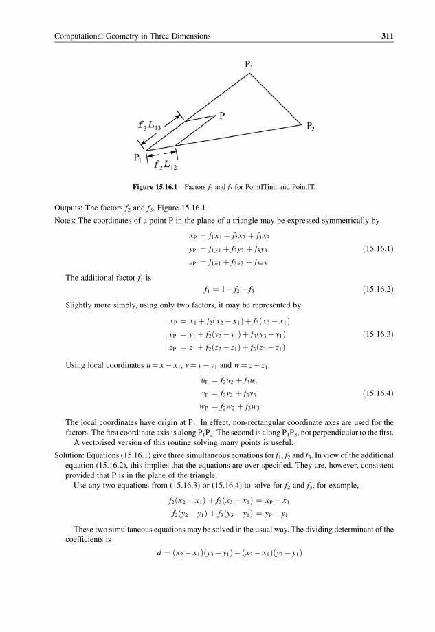
Outputs: The factors f2 and f3, Figure 15.16.1

Notes: The coordinates of a point P in the plane of a triangle may be expressed symmetrically by

xP ¼ f1x1 þ f2x2 þ f3x3

yP ¼ f1y1 þ f2y2 þ f3y3

zP ¼ f1z1 þ f2z2 þ f3z3

ð15:16:1Þ

The additional factor f1 is

f1 ¼ 1� f2 � f3 ð15:16:2ÞSlightly more simply, using only two factors, it may be represented by

xP ¼ x1 þ f2ðx2 � x1Þþ f3ðx3 � x1ÞyP ¼ y1 þ f2ðy2 � y1Þþ f3ðy3 � y1ÞzP ¼ z1 þ f2ðz2 � z1Þþ f3ðz3 � z1Þ

ð15:16:3Þ

Using local coordinates u¼ x� x1, v¼ y� y1 and w¼ z� z1,

uP ¼ f2u2 þ f3u3

vP ¼ f2v2 þ f3v3

wP ¼ f2w2 þ f3w3

ð15:16:4Þ

The local coordinates have origin at P1. In effect, non-rectangular coordinate axes are used for the

factors. The first coordinate axis is along P1P2. The second is along P1P3, not perpendicular to the first.

A vectorised version of this routine solving many points is useful.

Solution: Equations (15.16.1) give three simultaneous equations for f1, f2 and f3. In view of the additional

equation (15.16.2), this implies that the equations are over-specified. They are, however, consistent

provided that P is in the plane of the triangle.

Use any two equations from (15.16.3) or (15.16.4) to solve for f2 and f3, for example,

f2ðx2 � x1Þ þ f3ðx3 � x1Þ ¼ xP � x1

f2ðy2 � y1Þ þ f3ðy3 � y1Þ ¼ yP � y1

These two simultaneous equations may be solved in the usual way. The dividing determinant of the

coefficients is

d ¼ ðx2 � x1Þðy3 � y1Þ� ðx3 � x1Þðy2 � y1Þ

Figure 15.16.1 Factors f2 and f3 for PointITinit and PointIT.


Then

f2 ¼ ðxP � x1Þðy3 � y1Þ� ðyP � y1Þðx3 � x1Þd

f3 ¼ ðyP � y1Þðx2 � x1Þ� ðxP � x1Þðy2 � y1Þd

The second f could alternatively be solved by use of one of the equations in (15.16.4).

Comments: Note that even for a well-conditioned problem (a ‘good’ triangle, with points nowhere near in

line), data sensitivitymay result in an attempt to divide by zero; that is, d¼ 0may occur, or d very small

may occur, for example for a triangle parallel or nearly parallel to thexy plane. This is a data sensitivity.

The normal to the triangle has direction numbers given by the cross product (P2�P1)� (P3�P1).

In local coordinates this is given by

N ¼i j ku2 v2 w2

u3 v3 w3

��

so

N ¼ iðv2w3 � v3w2Þþ jðu3w2 � u2w3Þþ kðu2v3 � u3v2Þ

The third of these terms is

Nz ¼ k fðx2 � x1Þðy3 � y1Þ� ðx3 � x1Þðy2 � y1Þg ¼ kd

so, in themethod used in the example, the divisor is the z component of the normal to the triangle. This

gives the physical interpretation to the data sensitivity issue. Nz¼ d will be zero, or very small, when

the triangle normal is perpendicular, or nearly so, to the z axis.

Even for awell-conditioned problemwith a good triangle shape (the three defining points not near to

being on a straight line), the solution route must be correctly chosen. To avoid inaccuracy in critical

cases, calculate the components of the normal and select the one of largest magnitude. This indicates

which two equations from (15.16.3) will give the best solution route.

The triangle can be any shape, it does not require any identifiable direction, so itmay be equilateral if

desired.

15.17 Routine PointIT

Purpose: ‘Point In aTriangle’ – to obtain the point in a triangle given by the factors obtained byPointITinit.

The triangle may have moved in any way, but must retain its shape.

Inputs: Coordinates of the three new triangle points P1, P2 and P3, and the factors f2, f3

Outputs: The sought point P coordinates (xP, yP, zP)

Notes: The new triangle must retain its shape (the side lengths must be unchanged). The points must be

presented to PointITinit and PointIT in the same order. A vectorised version of this routine solving

many points is useful.

Solution: The desired point is given simply by

xP ¼ x1 þ f2ðx2 � x1Þþ f3ðx3 � x1ÞyP ¼ y1 þ f2ðy2 � y1Þþ f3ðy3 � y1ÞzP ¼ z1 þ f2ðz2 � z1Þþ f3ðz3 � z1Þ

which is the same as (15.16.3).


Comments: This uses the non-rectangular coordinate system of the triangle sides. See Section 15.16 for

further discussion. The symmetrical solution uses all three factors and three multiplications per

variable. However, it is probably more accurate in most cases to use the equations above.

15.18 Routine PointFPT

Purpose: ‘Point at the Foot of a Perpendicular into a Triangle’ – to obtain the coordinates of the foot of a

perpendicular from point P into the plane of a triangle P1P2P3

Inputs: Coordinates of the triangle points P1, P2, P3 and of the point P

Outputs: Coordinates of the foot point F, and the length LPF

Notes: None

Comments: The three points of the triangle define a plane, and this routine is just a pseudonym for

PointFPPl3P.

15.19 Routine Plane3P

Purpose: ‘Plane of 3 Points’ – convert to normal form (l, m, n, p)

Inputs: The coordinates of the three triangle points

Outputs: l,m, n, p – the direction cosines (l,m, n) of the normal to the triangle plane, and p, the length of the

normal from the origin to the plane in the direction (l,m, n). Usually the sign of p is positive, but the set

of four variables may have all signs reversed with valid results.

Notes: Arguably, one set (l,m, n, p) represents one surface of the plane, while (�l,�m,�n,�p) represents

the other surface, but this is not a significant issue here.

Solution: Consider any point in the plane, the point being at a distance L from the origin. Taking the dot

product of the point position vector (xP, yP, zP) with the plane normal (l, m, n) must give p¼ L cos u,where u is the angle between the position vector and the plane normal. Therefore, from the three points

of the triangle there are three equations, and there is also the direction-cosine interrelationship:

lx1 þ my1 þ nz1 ¼ p



l2 þ m2 þ n2 ¼ 1

ð15:19:1Þ

These are four equations for four unknowns, but the last equation is non-linear.

Practical solution can proceed as follows. Take the vector cross product

N ¼ ðP2 �P1Þ � ðP3 �P1Þ;to give the standard normal to the plane. In local coordinates on point P1 this is given by:

N ¼i j ku2 v2 w2

u3 v3 w3

��

so

N ¼ iðv2w3 � v3w2Þþ jðu3w2 � u2w3Þþ kðu2v3 � u3v2Þ

Normalise this vector by its length to give a unit vector N/len(N), which has the direction cosines

(l, m, n) of the plane. Then use one equation from (15.19.1) to obtain p, completing the solution.


Comments: There are no particular problems, provided that the triangle is well defined (points separated

and not in line).

15.20 Routine PointFP

Purpose: ‘Point at Foot of Perpendicular’ – to obtain the coordinates of the foot of a perpendicular from a

specified point P onto a normal-form plane.

Inputs: The plane normal-form parameters (l, m, n, p) and the point P coordinates

Outputs: The coordinates of the foot point F of the perpendicular, and the length of the perpendicular

Notes: The direction cosines have the property l2þ m2þ n2¼ 1.

Solution: The perpendicularmust have direction cosines (l,m, n). The length of the perpendicular is s from

P in the direction (l, m, n). This point has the coordinates

x ¼ xP þ ls

y ¼ yP þ ms

z ¼ zP þ ns

ð15:20:1Þ

The equation of the plane is

lx þ my þ nz ¼ p

By substitution,

ðxP þ lsÞlþðyP þmsÞmþðzP þ nsÞn ¼ p

Collecting terms,

ðxPlþ yPm þ zPnÞþ sðl2 þ m2 þ n2Þ ¼ p

giving

s ¼ p�ðxPl þ yPm þ zPnÞ ð15:20:2Þ

Substituting this value of s into equations (15.20.1) gives the coordinates of the foot F of the

perpendicular.

Comments: The solution is robust,with no particular problems.However, the direction of the normal is not

standardised (see the next routine).

15.21 Routine PointFPPl3P

Purpose: ‘Point at Foot of Perpendicular into a Plane of 3 Points’ – to obtain the coordinates of the foot of a

perpendicular from a specified point P onto a plane defined by three points. In practical suspension

analysis, this is the usual form of definition of a plane, and this has the advantage of giving a

standardised direction of the plane normal, essential for use in routines such as PointAT.

Inputs: Coordinates of the three points P1, P2 and P3 defining the plane, and of the point P

Outputs: The coordinates of the foot point F of the perpendicular, and the displacement along the standard

direction of perpendicular to give P from foot F

Notes: The direction cosines have the property l2þ m2þ n2¼ 1.

Solution: The perpendicular has direction cosines (l,m, n). The length of the perpendicular is s, possibly

negative, fromF to P in the direction (l,m, n). The direction of the normal is standardised in the positive

direction of the cross product

N ¼ ðP2 �P1Þ � ðP3 �P1Þ


It is convenient to use local coordinates (u, v, w) based on P1, for example,

u2 ¼ x2 � x1; v2 ¼ y2 � y1; w2 ¼ z2 � z1

The direction numbers of the normal are

LP ¼ v2w3 � v3w2

MP ¼ w2u3 �w3u2

NP ¼ u2v3 � u3v2

Dividing by theEuclidean length of this normal gives the direction cosines (l,m, n) of the plane normal.

For a displacement s from foot F to P in the positive normal direction, the position of F is given by

uF ¼ uP � ls

vF ¼ vP �ms

wF ¼ wP � ns

ð15:21:1Þ

The equation of the plane, which in local coordinates goes through the origin, is

lx þ my þ nz ¼ P

lu þ mv þ nw ¼ 0

By substitution,

lðuP � lsÞþ mðvP �msÞþ nðwP � nsÞ ¼ 0

giving

s ¼ luP þ mvP þ nwP ð15:21:2Þ

Substituting this valueof s into equations (15.21.1) gives the coordinatesof the footFof theperpendicular.

Comments: The solution is robust, with no particular problems. The direction of the normal is

standardised, which is very useful.

15.22 Routine PointATinit

Purpose: ‘Point “Above” a Triangle initialisation’ – to obtain factors for use by routine PointAT to

determine the position of a point relative to a triangle, the point being in any relative location (above,

below or in the plane of the triangle). The triangle may subsequently move in anyway, taking the point

with it, but the triangle must retain its shape.

Inputs: The coordinates of the defining points of the triangle in a knownposition, and the coordinates of the

point to be analysed

Outputs: Factors f2 and f3 (for the foot of the perpendicular; see Figure 15.22.1), and the directed out-of

plane distance s

Notes: A vectorised version of this routine solving many points is useful.

Solution:Drop theperpendicular fromP into the planeof the triangle, using routinePointFPT, giving the foot

pointF and the signedout-of plane distance s. Dependingonhow routinePointFPTiswritten, the signof s

may need to be changed here. The foot F may then be analysed by routine PointITinit to give f2 and f3.

Taking the cross product ofP2�P1 andP3�P1 in that order gives a vector perpendicular to the plane

of the triangle. This is the positive direction for the out-of-plane displacement s.

Comments: There is one new problem beyond the use of PointFPTand PointATinit, which is the sign of s,

which should be positive in the direction of the defined normal. This also requires that the normal


vector be calculated in the same way in PointATinit and PointAT, and that the triangle defining points

are presented to these routines in the same order.

15.23 Routine PointAT

Purpose: ‘Point “Above” a Triangle’ – to obtain the position of a point ‘above’ (i.e. relative to) a triangle

(above, below or exactly in the plane), using the factors obtained in an initial position by PointATinit

Inputs: The triangle point coordinates and the factors from PointATinit analysing the initial position

Outputs: The coordinates of P

Notes: This problem/routine is also sometimes known as ‘Pole-on-a triangle’, ‘Rod-on-a-triangle’ or,

consequently, just ‘Perch’. A vectorised version of this routine solving many points is useful.

Solution: Use the provided factors f2 and f3, Figure 15.22.1, to obtain a point in the plane of the triangle,

using routine PointIT. This is the foot F of the perpendicular from the point, so calculate the normal to

the plane by

N ¼ ðP2 �P1Þ � ðP3 �P1Þ

Move from F along this normal by a distance s (possibly negative), reaching P.

Comments: The order of vectors in the calculation ofNmust be the same as in PointATinit, or the out-of-

plane displacement will be reversed. There are no particular problems provided that the defining

triangle is good (points not in line). The points must be presented to PointATinit and PointAT in the

same order.

15.24 Routine Points3S

Purpose: To obtain the two points at the intersection of three spheres

Inputs: For each of three spheres, the coordinates of the centre and the radius

Outputs: The integer number of distinct real solutions, and the coordinates of the solution points

Notes: This is also known as the ‘Tripod’ problem or routine. If intersection does occur, the two solution

points are symmetrical about the plane of the centres. That is, the line from one solution to the other is

normal to that plane, and the mid-point of the line is a point in the plane, that is, the solutions are

equidistant from the plane. Various solution methods are possible, only one of which is given here.

Solution: The equation of a sphere has the basic form

ðx� x1Þ2 þ ðy� y1Þ2 þ ðz� z1Þ2 ¼ R21

Figure 15.22.1 Factors f2 and f3, and out-of-plane displacement s for PointATinit and PointAT.


The equations for the three spheres may be expanded to




ð15:24:1Þ

These are three independent non-linear simultaneous equations for the intersection point (x, y, z).

Subtracting any two of these equations removes the unknown non-linear terms, giving a linear

equation. If this is done in three pairs, the result is three linear equations. Unfortunately, such an

approach fails, because the three resulting equations are no longer independent.

The physical interpretation of this is instructive. Subtracting the equations of a pair of spheres

gives the equation of their radical plane. If the spheres intersect then the circle of intersection lies in

the radical plane. In the context of three spheres, any pair of the three radical planes intersect in a line

perpendicular to the plane of the centres. This line passes through the sphere intersection solution

points sought, and so all three pairs of radical planes have the same intersecting line, and so are not

independent. This applies geometrically and algebraically. In a numerical context, the radical planes

may bevery slightly skewed due to numerical imprecision, inwhich case their intersection is a single

point. However, this is not a useful point because although it is on the desired line of the solutions it is

positioned along the line in an effectively unpredictable way, depending on the minutiae of the

numerical calculation. A different solution strategy must therefore be sought.

One good method of solution is to obtain only two radical planes, say for S1–S2 and S1–S3, and to

intersect these for a line through the solution points. Then intersect this line with any of the sphere

equations, say S1, to obtain the two points.

Using local coordinates based on the centre of sphere 1, (u¼ x� x1, etc), the three sphere

equations become:

u2 þ v2 þw2 ¼ R21 ¼ c1 ð15:24:2Þ

u2 þ v2 þw2 � 2u2u� 2v2v� 2w2w ¼ R22 �ðu22 þ v22 þ w2

2Þ ¼ c2 ð15:24:3Þ

u2 þ v2 þw2 � 2u3u� 2v3v� 2w3w ¼ R23 �ðu23 þ v23 þ w2

3Þ ¼ c3 ð15:24:4Þ

The radical planes S1� S2 and S1� S3, by subtraction, are

u2u þ v2v þ w2w ¼ 1

2ðc1 � c2Þ ¼ c4 ð15:24:5Þ

u3u þ v3v þ w3w ¼ 1

2ðc1 � c3Þ ¼ c5 ð15:24:6Þ

These two equations may be used to eliminate two variables. Say eliminate w first, using w3(15.23.5) –

w2(15.23.6) to give

uðw3u2 �w2u3Þþ vðw3v2 �w2v3Þ ¼ w3c4 �w2c5

Now write

a1 ¼ w3u2 �w2u3

a2 ¼ w3v2 �w2v3

a3 ¼ w3c4 �w2c5


Then using

a4 ¼ a3

a2; a5 ¼ �a1

a2

the relationship between v and u can be simply expressed as

v ¼ a4 þ a5u ð15:24:7Þ

where the constants are known. Now using equation (15.23.5),

u2u þ v2ða4 þ a5uÞþw2w ¼ c4

uðu2 þ a5v2Þþw2w ¼ c4 � a4v2

This gives a simple linear equation for w(u) with known coefficients:

w ¼ b1 þ b2u ð15:24:8Þ

Equations (15.24.7) and (15.24.8) can be substituted into (15.24.2) to give a quadratic equation in u

only, so the problem is effectively solved, producing potentially twovalues for u, with corresponding

values for v and w then solved by the subsequent equations. If the quadratic equation produces no

real solutions, then the spheres do not have the required intersection (possibly two of them domeet).

If the quadratic equation produces one real solution (i.e. coincident real solutions of the same value),

then the intersections are coincident. This would occur, for example, when two spheres just touch at

a single point, and the third sphere intersects the first two, passing exactly through the touching

point, or, seen in another way, two spheres intersect in a circle with the third sphere just touching the

circle. In the case of suspension analysis, the expected result would be two separate real solutions,

indicating the expected two possible physical intersections. Given the two u solution values, uA and

uB, then equations (15.19.7) and (15.19.8) give the other coordinates, providing the complete

solutions (uA, vA, wA) and (uB, vB, wB).

Comments: One of these two solutions will be the desired one. The other corresponds to a geometrically

correct but physically inappropriate assembly of the components. The correct solution must subse-

quently be selected carefully if problems are to be avoided, but this is not the province of routine

Points3S, which lacks the necessary extra information to select the desired solution from the two

candidate points.

As with some other routines, it will be noticed here that there are several possible solution paths, with

possible data sensitivities according to the alignments, even for a basicallywell-conditioned problem. The

crucial point is the order of elimination of the variables, which should be based on the avoidance of

divisors of small magnitude (i.e. select the solution route with the largest magnitude divisors).

15.25 Routine Points2SHP

Purpose: ‘Points at the intersection of 2 Spheres and a Horizontal Plane’

Inputs: Coordinates of the centres of the two spheres and corresponding radii, and the z value of the

horizontal plane zHP

Outputs: The integer number of real solutions found and the solution point coordinates

Notes: The solution of an independent suspension conveniently begins with a position of the lower outer

ball joint. This could be done by specifying the rotation of the lower arm, but is easily done by

specifying the height of the ball joint, which is approximately related to the suspension bump value,

then solving for the x and y coordinates according to the arm geometry.


Solution: The equations to be satisfied are two spheres and a horizontal plane:

ðx� x1Þ2 þðy� y1Þ2 þðz� z1Þ2 ¼ R21 ð15:25:1Þ

ðx� x2Þ2 þðy� y2Þ2 þðz� z2Þ2 ¼ R22 ð15:25:2Þ

z ¼ zHP ð15:25:3Þ

In local coordinates, u¼ x� x1, etc., and substituting z¼ zHP,

u2 þ v2 þw2 ¼ R21

u2 þ v2 þw2 � 2u2u� 2v2v� 2w2w ¼ R22 �ðu22 þ v22 þw2

2Þ

w ¼ wHP ¼ zHP � z1

There are potentially two circles of intersection of the spheres with the plane, with equations given by

substituting for w:

u2 þ v2 ¼ R21 �w2

HP ¼ c1

u2 þ v2 � 2u2u� 2v2v ¼ R22 �ðu22 þ v22 þw2

2Þ�w2HP þ 2w2wHP ¼ c2

Subtraction of these two circle equations gives the equation of the radical line:

2u2uþ 2v2v ¼ c1 � c2

Choosing to eliminate u first,

v ¼ � u2

v2u þ c1 � c2

2v2ð15:25:4Þ

where division by v2 is required. If the absolute value of u2 exceeds that of v2, it is better to eliminate u

first, with

u ¼ � v2

u2v þ c1 � c2

2u2ð15:25:5Þ

Substituting one of these two options into (15.24.1) or (15.24.2) gives a quadratic equation in one

variable. The other then follows from (15.24.4) or (15.24.5).

Comments: The physical interpretation of this is that substituting the constant plane height into the sphere

equations gives the equations of two circles in the plane (prospectively). The intersection of the two

circles is a simpler two-dimensional problem, easily solved. Equations (15.20.4) and (15.20.5) are

alternative equations for the radical line of the two circles. If this line is exactly or nearly parallel with

the v axis (y axis) then solve for v first because v(u) is badly conditioned. In this case, eliminate u, with

(15.20.5), solving for v, because abs(u2)> abs(v2).

15.26 Routine Point3Pl

Purpose: ‘Point in 3 Planes’ – to obtain the intersection point of three planes, each plane being specified by

any one point in the plane and the direction cosines of the normal to the plane.

Inputs: For each plane, the coordinates of one point in it, and the direction cosines of its normal, for

example (x1,y1,z1) and (l1, m1, n1)


Outputs: The coordinates of the one intersection point (xP, yP, zP)

Notes: This routine is required for three-dimensional velocity diagram analysis of the Points3S (‘Tripod’)

problem.

Solution: The solution point must lie in each plane, so satisfying simultaneously, by dot products,

l1xP þ m1yP þ n1zP ¼ l1x1 þ m1y1 þ n1z1 ¼ c1



These are three simultaneous linear equations in xP, yP and zP, conveniently solved by use of a general

simultaneous equation solver (e.g. Routine SimEqns).

Comments: In the case of a suspension, the practical problem would always be well conditioned, but data

sensitivities could easily arise due to critical alignments of the planes with the axes. A Gaussian

elimination solver with pivoting will correctly negotiate such problems, and produce a good solution.

Alternatively, use an ad hoc solver by the usual methods, with the order of elimination of the variables

chosen to avoid small divisors.

15.27 Routine ‘PointLP’

Purpose: ‘Point of a Line and a Plane’ – to obtain the coordinates of the point of intersection of a general

parametric-form line and a normal-form plane

Inputs: The parametric variables of the line, and the normal form variables of the plane

Outputs: The coordinates of the intersection point

Notes: None

Solution: At the line parametric point S, the line coordinates are

x ¼ xL þ lLs

y ¼ yL þ mLs

z ¼ zL þ nLs

ð15:27:1Þ

The equation of the plane is

lPx þ mPy þ nPz ¼ pP

By substitution,

lPðxL þ lLsÞþmPðyL þ mLsÞþ nPðzL þ nLsÞ ¼ pP

Collecting terms and making s the subject,

s ¼ pP �ðxLlP þ yLmP þ zLnPÞlPlL þ mPmL þ nPnL

ð15:27:2Þ

The divisor will be recognised as the dot product of the plane normal and the line direction.

Substituting the resulting value of s into equations (15.26.1) gives the desired coordinates.

Comments: The solution is not completely robust. The dot product could cause a division by zero.

Physically, if the dot product is zero then the plane normal and the line are perpendicular, in which case

the line and plane will not meet, that is, will meet at infinity. If the defining point of the line is in the

plane, the value of s is zero, which is not problematic. If the point is in the plane and the dot product is


zero then the numerical solution for s is 0/0, but 0 would usually be an acceptable value. Therefore

evaluate the numerator first. If this is not zero, evaluate the denominator. If this is zero, return an

indicator of this situation. One way to handle such infinities is homogeneous coordinates.

15.28 Routine Point3SV

Purpose: To obtain the velocity of a point positioned by three rods (the position of which is found by

Points3S)

Inputs: The coordinates of the three locating points, the coordinates of the apex point, and the velocity

components of the three base points

Outputs: The velocity components of the apex point (uP, vP, wP)

Notes: None

Solution: In the 3D velocity diagram, each base point has a givenvelocity point. Relative to the base point,

the other-end velocity is tangential only. Relative to the base velocity point, then, the solution point

must be in a plane with a normal given by the rod axis direction cosines. The solution velocity is the

therefore the intersection in the velocity diagram of the three such planes, one for each rod.

The first rod has base coordinates (x1, y1, z1). The apex position is (xP, yP, zP). From these, the first rod

direction cosines are easily determined. Similarly for the others.

For each rod, the base point velocity, for example (u1,v1,w1), and the corresponding direction cosines,

for example (l1,m1,n1), give a plane in the three-dimensional velocity diagram with an equation such as

l1u þ m1v þ n1w ¼ l1u1 þ m1v1 þ n1w1 ¼ c1

This gives three simultaneous linear equations in the velocities (u, v,w). The intersection of the three

planes can be solved by the use of routine Point3Pl.

Comments: Routine Point3Pl will obtain the intersection point, called with the correct arguments.

Although velocities are being solved for, this requires a geometric construction in ‘velocity space’, that

is, in the three-dimensional velocity diagram.

15.29 Routine PointITV

Purpose: ‘Velocity of a Point In a Triangle’ – to obtain the velocity of a point in the plane of a triangle,

given the triangle corner velocity components and the point position factors f2 and f3

Inputs: The corner velocity components for the triangle, for example (u1, v1, w1), and the point position

factors f2 and f3 (found by PointITinit)

Outputs: The point velocity components

Notes: The triangle must retain its shape and order of defining points, but may move in any way. The

velocities of the corners of the triangle must be compatible, with the side lengths remaining constant.

The variables (u, v, w) here are velocities, not local positions.

Solution: By differentiation to give velocities from positions, it is evident that the velocity of the point is

given in terms of the triangle corner velocities by the same factors as is its position in terms of the corner

positions. The required factors are found by PointITinit, so

uP ¼ u1 þ f2ðu2 � u1Þþ f3ðu3 � u1ÞvP ¼ v1 þ f2ðv2 � v1Þþ f3ðv3 � v1ÞwP ¼ w1 þ f2ðw2 �w1Þþ f3ðw3 �w1Þ


Comments: The solution is straightforward, other than that caution is required to provide only compatible

velocities of the three base points. Thevelocities of two ends of a rigid rodmust have equal components

along the rod. This longitudinal velocity is the dot product of the complete velocity with the rod

direction cosines, so for two ends A and B the condition is

luA þmvA þ nwA ¼ luB þmvB þ nwB

15.30 Routine PointATV

Purpose: ‘Velocity of Point Above Triangle’ – to calculate the velocity of a point with a position specified

relative to a rigid triangle, above, below or exactly in the plane of the triangle

Inputs: The coordinates of the triangle corners, the factors f2 and f3 and the out-of-plane displacement s of

the point P (from routine PointATinit), and the velocity components of each defining corner of the

triangle (which velocities must be compatible)

Outputs: The velocity components of the point

Notes: This routine is used for three-dimensional velocity diagram analysis for points with position

defined by PointAT.

Solution: The coordinates of P1, P2 and P3 are given. Also the factors f2 and f3 for F and the out-of-plane

displacement s for P. The foot F of the perpendicular from P has coordinates solved by routine PointIT,

using f2 and f3. The coordinates of P are solved by routine PointAT. Therefore all positions are known.

The velocity of F is calculated by routine PointITV, using the factors f2 and f3.

It remains to calculate the velocity of P relative to F. Length LPF is constant, so the relativevelocity

is purely tangential. Drop a perpendicular from P1 onto line P2P3 with foot P4. The velocity VP/F of

P relative to F is parallel to the plane, with the components shown,VT1 being parallel to line P1P4 and

VT2 being parallel to line P2P3, Figure 15.30.1. The velocity of P4 can be found from the velocities

of P2 and P3 by linear interpolation or extrapolation according to the position factor of P4 along

P2P3 (P4 may be outside P1P3, with f4< 0 or f4> 1).

Calculate the unit normal to the plane for F towards P. By dot products with this unit vector, the

normal (out-of-plane) velocity components at each point, VN1,VN2,VN3 andVN4, can be determined,

as seen in the figure.

The angular velocity of the triangle may be considered in three components. The first is the in-

plane rotation, about an axis perpendicular to the plane, which has no effect on VP/F, so will not be

Figure 15.30.1 Tangential velocity componentsVT1 andVT2 for the point P relative to F, derived from the out-of plane

velocities VN1 etc. at each corner.


considered further. The right-hand angular velocity about any axis parallel to the line P2P3 is

V1 ¼ VN1 �VN4

L14The first tangential velocity component is then

VT1 ¼ V1LFP ¼ ðVN1 �VN4ÞLFPL14

Now, to obtain the second tangential component, the angular velocity about an axis parallel to P4P1 is

V2 ¼ VN2 �VN3

L23

giving

VT2 ¼ V2LFP ¼ ðVN2 �VN3ÞLFPL23

The velocity of P now follows by the addition of the two tangential components to VF.

Comments: The solution is basically robust, with divisions by lengths that must be non-zero in practical

cases. The solution is not symmetrical in the use of the three points of the triangle, and the in-plane

perpendicular could equallywell be dropped fromone of the other corners. The end result forVP should

be the same.

The solution is straightforward in concept, but more detailed than other routines here, and care is

needed to ensure a correct implementation. In practice, the accuracy is very good. A point to be careful

about is that the corner input velocities must be compatible (the base triangle is rigid).

When the point P is safely out-of-plane, routine Point3SV could be used. However, this is

unsatisfactory for in-plane points, and is really intended for configurations in which the point position

is solved by Points3S. When the triangle is rigid, routine PointATV here is the appropriate solution

method.

15.31 Rotations

The rotational position of a solid body can be represented and solved by the use of points on the bodywith

vector analysis, and this is generally considered to be the practical method, using routines such as those

described above. It is particularly suitable for mechanism analysis, such as that for suspensions, which

tends naturally to deal with specific points on each member. An interesting alternative is the use of

quaternions. These are particularly suitable for use on isolated solid bodies, such as aircraft or spacecraft,

but could possibly be usedwith advantage for some three-dimensionalmechanismor suspension analyses.

Appendix D gives an explanation of the properties of quaternions and their use.

————— // —————


16

Programming Considerations

16.1 Introduction

This chapter deals with some particular issues in programming that bear upon the solution of suspension

geometry. Some of these issues are fairly specific to suspensions (e.g. the ‘assembly’ problem of selecting

one of two or more prospective solutions for a point), while others are more general (e.g. generally good

programming practice). Three-dimensional geometrical programs are of sufficient complexity that the

best programming practices are really needed to achieve reliable success.

16.2 The RASER Value

The RASER value for software is a reliability, accuracy, speed and ease of use rating. The reliability of a

subroutine is primarily its ability to survive without crashing in any data environment, and depends on its

failuremodes analysis.Accuracy can be divided into accuracy for ‘normal’ cases and accuracy for difficult

cases. Speed again can be divided into speed on normal cases and speed for difficult cases. Ease of use of a

subroutine basically depends on its argument list.

The idea behind a RASER value is to draw attention to the quality of a piece of software. Just being

conscious of the concept will concentrate a programmer’s mind, the idea that his program might actually

be quantitatively scored evenmore so. Such a scoring systemworks basically as follows. Program quality

is on a scale from0 to 1.A notionally perfect program scores 1.000000, but in practice no program is above

some improvement. The maximum total score available is in fact 0.999999.

The first 9 is for reliability and ease of use. Reliability means not crashing, whatever the data values.

With bad (‘impossible’) data, the correct error state IE values must be returned (Section 16.3). Ease

of use depends on a suitable routine name, and a considered arrangement of the argument list

(Section 16.9).

The second 9 is for accuracy on typical cases (i.e. the easy ones). The third 9 is for speed on such

cases.

The fourth 9 is for accuracy on the occasional particularly difficult cases. The fifth 9 is for speed on

such cases. Difficult cases include problems with bad conditioning and ones with data sensitivity

problems.

The sixth 9 is for code compactness. Actually, this was once very important, in the early days of small

computer memories, but is not so important nowadays for numerical software, which tends to be small

anyway. However, there is much obese software around, so a low score is a possibility here.


Evidently, a score of 0.911111 beats a score of 0.899999. Reliability is more important than any other

aspect.

These topics are dealt with in more detail in subsequent sections.

16.3 Failure Modes Analysis

Failure modes analysis was developed to improve the overall performance and reliability of large

commercial and military systems, these being sufficiently unpredictable due to complexity or adverse

influence that complete reliability could not be assured. Then, instead of simply accepting occasional

failure and its consequences, the idea of design for operation under conditions of partial failure was

introduced. Thiswas by nomeans new, in fact, as engineering design had included it in one formor another

for many years, including, for example, plastic failure design techniques.

The basic idea behind failuremodes analysis is to accept that failuremight or will sometimes occur, and

to anticipate the likely forms of such failure and to be prepared for them, that is, to be aware of the

prospective failure modes and to ameliorate the damage. This concept is readily applicable to computer

software design, with fruitful results.

Program or subroutine outcomes may be classified as follows:

(1) a program ‘crash’;

(2) solution claimed good, is good;

(3) solution claimed good, is bad;

(4) solution failure stated, but actually good solution possible;

(5) solution failed, failure admitted.

To some extent this depends on the problem.Avery difficult problemmay require an inordinate amount of

time, in which case it may be appropriate to abandon the attempt. It is widely accepted that the worst

outcome is (3), a claimed good solution that is actually bad. Result (4), failing to find an achievable

solution, is not ideal, but may be acceptable. The programmay work well on normal problems, but it may

not work on some particularly difficult cases. If the difficult case are rare, the programmay still be useful.

And, of course, it may simply not be known how to solve the difficult cases. The programmay also fail by

doing the computations but losing accuracy in some way. These issues are dealt with in subsequent

sections.

It is usual for a numerical program to include at the end of its argument list an integer variable IE or Ierr,

which is used to indicate its ‘failure status’, or, in modern sales parlance, its ‘success status’. IE¼ 0

indicates no undue problems and a claimed good result, with other values giving an indication of less

satisfactory outcomes. Typically a routine will have an output code along these lines:

IE = 0 Good result.

IE = 1 Data outside acceptable range.

IE = 2 There is no solution.

IE = 3 Accuracy lost.

IE = 4 SQRT unexpected negative argument.

IE = 5 ASIN or ACOS argument out of range.

IE = 6 LOG argument out of range.

IE = 7 Division by zero.

IE = 8 Failed to converge in iteration.

IE = 9 Points must not be in line.

IE = 10 Problem in lower subroutine call.

IE = 11 . . .


16.4 Reliability

Reliability in a broad sense is the ability of a program to exit gracefully whilst not making unreasonable

claims about its results. In a narrower sense, as dealt with in this section, reliability is the ability of

a program to keepworking, not crashing, regardless of the data presented to it. Thismeans anticipating any

problems and dealing with them in advance, rather than being a passive subject of difficulties. The main

problems in this regard are IE items 4–7 in the list of the previous section.

In a simple program, IE items 4–6 will cause a program termination – a ‘crash’. In many languages,

so will item 7. In Fortran, item 7 gives a result of infinity, which is a mixed blessing, at best. If the

program terminates, then data may be lost, for example several minutes of typing in suspension

coordinates, which is invariably undesirable. This problem is easily solved. Whenever one of these, or

any other ‘risky’ routine, is to be used, first test the argument for acceptability. To a neophyte

programmer, this may seem a nuisance, but experienced programmers know that in the end taking the

trouble to do this saves a good deal of time and frustration. The number of occasions on which it is

needed is not very great.

For example, the code fragment, all in real numbers

x=sqrt(a**3-d**3+f-g)

is risky, for two reasons. Even if the data supplied are good, it is hard to anticipate the outcome of the

calculation of the argument value. Of course, there may be additional information available to the

programmer to indicate that this value ‘cannot’ be negative. However, the arguments supplied may be

outside the allowed range. If these have not been checked at the outset, the argument may be negative in

defiance of the ‘known-to-be-positive’ value. The solution is simple:

xsq = a**3-d**3+f-g

If (xsq<0) Goto 14

x = sqrt(xsq)

where label 14 is in an error block at the end of the routine, such as

14 Pause ’Negative Sqrt argument.’ ; Stop

The failure is anticipated, and dealt with in a civilised manner, according to the programmers wishes.

Similarly,

If (a<1 .or. a>1) Goto 15

x = asin(a)

. . .

If (b<0) Goto 16

x = log10(b)

. . .

If (c==0) Goto 17

x=(p+q)/c

. . .

! Error block:

14 IE=4 ; Return

15 IE=5 ; Return

16 IE=6 ; Return

17 IE=7 ; Return

Programming Considerations 327

16.5 Bad Conditioning

If equations are badly conditioned then they cannot be solved accurately by any method. Typically this

arises with simultaneous equations where, say, there are two equations each representing one line. If

the lines are at a very small angle to each other then the accuracy of the solved point is poor in the

direction along the lines. This is a distinct problem from general ‘data sensitivity’, which can occur

even if the problem is basically well conditioned. In short, if the problem is badly conditioned then

there is no way to ensure accurate results, compared with a well-conditioned case. If the problem is

well conditioned, then accurate results are possible, but not necessarily by one particular method of

solution. The quality of the solution will depend on the method used, which must be selected correctly

according to the particular data.

Consider the problem of two linear simultaneous equations in variables (u, v):

l1uþm1v ¼ p1 ð16:5:1Þ

l2uþm2v ¼ p2 ð16:5:2Þ

Physically, this arises, for example, in the two-dimensional solution of the velocity of the joint of two rods

of known length and position and specified base velocities. These equations are badly conditioned if they

are almost the same equation, that is, if the coefficients are in almost exactly the same ratios. Just

multiplying one equation by a constant does not change the conditioning. If l1¼ l2 andm1¼m2 and p1 is

similar in value to p2, this would be parallel lines at a close spacing, actually not meeting. Now if, say, l2 is

changed slightly, the lines will meet at a very small angle. This is bad conditioning. The constants may all

be different, but nearly the same, and it is still bad conditioning. Consider the case when the lines are

roughly parallel with the x axis, and meet at a small angle. A small change in the constant p for one

equation will make a large difference in the x value of the solution. More precise calculations will not

necessarily help – if the actual physical data are of limited accuracy then the true value ofxwill actually be

known only within wide limits.

To solve the equations, we can eliminate one variable, say u, by using l2(16.5.1) – l1(16.5.2) to give

uðl2l1 � l1l2Þþ vðl2m1 � l1m2Þ ¼ l2p1 � l1p2

giving the solution as

v ¼ l2p1 � l1p2

l2m1 � l1m2

ð16:5:3Þ

or solve for u by the same method as for v, using elimination of v by m2(1) – m1(2) to give

u ¼ m1p2 �m2p1

l2m1 � l1m2

ð16:5:4Þ

In either (16.5.3) or (16.5.4) it is apparent that if the matching coefficients are similar in value then the

numerator and denominator will be small, and both will be subject to inaccuracy due to subtractive

cancellation. The problem is badly conditioned, and there is little that can be done to help, short of using

quadratic precision numbers, and although that would reduce the problem of the numerical errors, the

problem of the large effect of small changes in the data would remain. Fortunately, in practical suspension

analysis the geometrical problem must be basically well conditioned or the suspension itself will be

ineffective as a structure, with hopelessly bad location, say due to bad triangulation.


16.6 Data Sensitivity

Consider again the problem of two linear simultaneous equations in variables (u,v):

l1uþm1v ¼ p1 ð16:6:1Þ

l2uþm2v ¼ p2 ð16:6:2Þ

Solving for v first gave

v ¼ l2p1 � l1p2

l2m1 � l1m2

ð16:6:3Þ

There are now three ways to solve for the other variable, u. We can substitute for the known v value into

equation (16.6.1) or (16.6.2), giving

u ¼ p1 �m1v

l1ð16:6:4Þ

or

u ¼ p2 �m2v

l2ð16:6:5Þ

or solve for u by the same method as for v, using elimination of v by m2(16.6.1)�m1(16.6.2) to give

u ¼ m1p2 �m2p1

l2m1 � l1m2

ð16:6:6Þ

The divisor in equations (16.6.3) and (16.6.6) is

d ¼ l2m1 � l1m2 ð16:6:7Þ

Consider now a well-conditioned case. Then the divisor d is then not unreasonably small, and

equation (16.6.3) will evaluate v accurately. However, it may be that, say, the direction cosine l1 is

small, in which case equation (16.6.4) will be near to 0/0, and inaccurate. In fact, l1 may actually be zero,

and equation (16.6.4) may be incapable of solving the problem at all, even though the problem is well

conditioned. This is a data sensitivity. It could arise physically simply because one of the rods is parallel to

an axis; for example, in this case rod 1 parallel to the v axis, giving m1¼ 1 and l1¼ 0. The difficulty is

purely due to the method of solution attempted, it is not fundamental to the problem. Using instead

equation (16.6.5) may give a good solution, or, for other data values, may instead be a problem.

Equation (16.6.6) depends on the value of d rather than on the individual alignments, so depends only on

the conditioning. To avoid unnecessary problems, in this case it is probably best to evaluate d once and to

use equations (16.6.3) and (16.6.6).

If problems arise in a basically well-conditioned problem, it is due to the use of a coordinate system that

aligns in a troublesome way with the physical configuration. In the above problem, using equa-

tions (16.6.3) and (16.6.6) as the method is equivalent to using rotated coordinates so that the quality

of the solution depends only on the conditioning; that is, awell-conditioned problem cannot then have any

‘bad alignments’.

A related general rule of alternative evaluations is to use the one with the largest divisor, thereby

minimising the risk of attempting 0/0 or something close to it.


In a problem of two linear simultaneous equations, the basic physical analogue is the intersection of two

lines in a plane. For three linear equations, it is the intersection of three planes in a three-dimensional

space. Similar problems to the above may arise in such cases, and may be dealt with in similar ways,

basically by avoiding small divisors as far as possible, choosing a solution routewith the largest ones. The

solution route may therefore have to be determined according to the particular data values.

Another good example of data sensitivity is the problem of deducing the interpolation factor f for a

point P known to lie on a line P1P2, with all coordinates known. The value of f is given by

f ¼ xP � x1

x2 � x1¼ yP � y1

y2 � y1¼ zP � z1

z2 � z1ð16:6:9Þ

Any one of thesemay give the required result, in general, but any one of them could easily fail because the

line P1P2 happens to be parallel to one of the axes, causing a division by zero. There are twogood solutions.

As usual, one method is to avoid a small divisor, so, assuming here actual separation of the points P1and P2,

If (abs(x2-x1) > abs(y2-y1) .and. abs(x2-x1) > abs(z2-z1)) then

f = (xp-x1)/(x2-x1)

elseif (abs(y2-y1) > abs(z2-z1)) then

f = (yp-y1)/(y2-y1)

else

f = (zp-z1)/(z2-z1)

endif

will select the best equation to use, giving reliability and the best accuracy. Admittedly, however, it is

rather bulky. Another possibility is to use

f = Len1P/Len12

which is coordinate independent. This will work unless L12 is zero, but that case is not useful

anyway. Whether this is a better option really depends on whether the relevant lengths are already

known or not.

16.7 Accuracy

A ‘blunder’ in a calculation is when there is a wrong operation performed or a wrong number used. A

blunder would be, for example, a program error such as a plus sign where there should be a minus sign, or

the wrong variable name used, or an incorrect solution chosen, as in Section 16.10. When there is a

blunder, the answer is completely wrong, becoming meaningless. In contrast, mathematically or

statistically speaking, an ‘error’ in a calculation is a small inaccuracy due to limited precision of the

numbers, or the accumulation of small errors by successive numerical processes.

Setting aside gross inaccuracies due to blunders, which are up to the programmer to eliminate by care

and testing, the accuracy of the computational results depends on the inherent precision of the variable

representation used and on the skill of the programmer in avoiding inaccuracy-introducing processes.

In the early days, the representation of real numbers was far from standardised. Many early computer

languages represented the real numbers by a 4-byte word, that is, 4� 8¼ 32 bit representation. This is a

scientific representation with several of the binary bits used for the exponent value, the remainder for the

‘mantissa’ or ‘characteristic’, the actual sequence of digits. In decimal terms, a 4-byte number has a

precision of about 7 decimal digits. Some specialised scientific computers used a 60-bit representation

with greater precision.


Fortran introduced a ‘double precision’ real variable usually of 64 bits. This was not completely

standardised at the time because of the interests of the various hardware manufacturers. However, this is

now commonly available in Fortran and C and other languages.

The Basic language varies considerably from one implementation to another. Many Basics have had

4-byte real numbers, some have had 5-byte reals, and more recently some have had 8-byte real numbers.

Basic also introduced the ‘numeric’ data type of 8 bytes storage (64 bits), which is used for both integers

and reals. One bit is used to indicate whether the number being represented is a real or an integer, so the

precision of the reals is reduced by one bit compared with a true 64-bit real representation. This is simpler

for beginning programmers, who no longer have to bother about the distinction between integer and real

numbers, but is inefficient, andmost scientific programmers prefer to keep a clear distinction, particularly

because the two types of number do different jobs.

Themodern IEEE real number standard gives 53-bit precision, the other bits being used for the sign and

the exponent value. The 53 bits give about 16 decimal digits of precision, so 8-byte real numbers are held to

a remarkably close figure. On a bar 1 metre long, this is 10�16m, which may be compared with the

diameter of an atom, about 0.1 nm (10�10m), or the diameter of an atomic nucleus, which is about

10�15m. Such a precise representation evidently does not really havemuch physicalmeaning, and is there

for a different reason, to ensure that the ultimate result of a long calculation with accumulating

inaccuracies can still result in a useful final value. It has been said with justification that to an engineer

the precision is 3 useful decimal digits with 13 guard digits.

Quad-precision numbers use a 16-byte representation, and have about 35 decimal digits of precision.

The amount of calculation in a suspension is such thatwith 8-byte real numbers a final precision of about

1 part in 1012 can normally be achieved. This is far more accurate than has physical significance. If the

results areworse than this then either the problem is a particularly awkward one, due to poor conditioning,

or, more likely in practice, the problem has a data sensitivity and the program is solving it by a poor

method. Methods that work around data sensitivities by selecting the solution route with the largest

divisors produce the most accurate results, as described in Section 16.6. Because of the remarkable

precision of the 8-byte real numbers now in common use, data sensitivities often have only a limited

impact, but care in avoiding such problems is still the sensible approach.

16.8 Speed

In the early days of computing, the speed and efficiency of software were of paramount importance.

Computers were slow, and very unreliable because of the thermionic valves. Programs had to run fast to go

to completion before a valve failure. The introduction of transistors greatly improved reliability, and large-

scale integration has subsequently produced personal computers of amazing speed and memory capacity.

The analysis of one position of a suspension can now be done in microseconds, so there is no longer any

need for a program to be efficient, it will seem to run instantaneously anyway. It must be said that in a

professional context, the logical thing to do is to minimise the programmer time, not the computer time.

Another way to view this is that the programmer’s time should be spent on making the program reliable

and accurate, rather than fast.

Nevertheless, it remains true that it is very satisfying tomost programmers towrite an efficient (i.e. fast)

program.As long as this is not to the detriment of reliability and accuracy, there is probably no harm in this,

and if the routine is one that will be used numerous times, it may be beneficial. However, starting writing a

programwith speed as the main factor is likely to lead to problems. It is best to write the program initially

for clarity, to be sure that it really does do the job correctly. Later, when it is working, it could be polished

up for speed. There are two rules of optimisation sometimes quoted:

(1) Do not optimise for speed.

(2) If you must do it, do not do it yet.


The reason for this is that a really speed-optimised programmay be unclear in operation, causing issues of

reliability and maintenance.

Most programs have ‘hot spots’ – parts where the greater part of the work is done, usually in the

innermost loops. The best way to improve the performance of an existing program is to polish up the

efficiency of the hot spots only, and leave the rest as simple and clear as possible.

Such tactical optimisation is very secondary to strategic optimisation, which is to choose an efficient

algorithm in the first place. In the case of suspension geometry, the strategic optimisation is to use true

analytic geometric solutions where possible, rather than iterative solutions, which are generally much

slower.

16.9 Ease of Use

Ease of use depends on a suitable routine name, and a considered arrangement of the argument list. There

is no absolutely correctway to do this, but long ago itwas found that the sensible arrangement is to have the

incoming data firstwith the results later, generally to have integers before reals, but to put control variables

at the end. In individual cases, judgement is needed. For example, an integer carrying the value of the

declared size of an array might reasonably be placed just before the array name, rather than collected

together with other integers away from the array name.

16.10 The Assembly Problem

Some routines return more solutions than apply physically to the problem, a difficulty that can certainly

arise in the case of suspension geometry analysis. A good example is the routine Points3S, solving the

position at the apex of three rods of known length and known base positions (Section 15.24). This is

frequently required for suspension geometry, and there is only onevalid solution for the actual suspension.

However, the routine returns two equally valid geometrical solutions. The problem is to choose the one

that is appropriate to the physical problem.

As a specific example, consider the solution of the upper ball joint, based on the upper arm pivot

points, P4 and P5, and the lower ball joint P3. The three rod lengths are known. Routine Points3S solves

the geometric problem using a quadratic equation which gives two solutions. This is geometrically

correct – there are indeed two points that satisfy the equations. One point is the desired one. The other

solution found is one that is on the opposite side of the plane of the base points, Figure 16.10.1. The

routine calling Points3S and using its results has the problem of selecting the desired solution in some

way. In this case there are several possibilities. One is to choose the solution that is nearest to the

original (static) position, by calculating two lengths. Actually, there is no need to calculate the actual

lengths, the two square root operations can be avoided by comparing the squares of the lengths.

Denoting the static positions as (xs,ys,zs) and the moved position as (x,y,z) this would be implemented

as follows:

Call Points3S(. . . ,xa,ya,za,xb,yb,zb . . .)

len1sq=(xa-xs(6))**2+(ya-ys(6))**2+(za-zs(6))**2

len2sq=(xb-xs(6))**2+(yb-ys(6))**2+(zb-zs(6))**2

If(len1sq<len2sq)then

x(6)=xa ; y(6)=ya ; z(6)=za

else

x(6)=xb ; y(6)=yb ; z(6)=zb

endif


This usually works satisfactorily, but consideration should be given to the possibility, in general geometry

at least, that in an extreme displacement, at very large bump, this could fail, because the wrong point

becomes closer.

Considering Figure 16.10.1 again, a good alternative could be to apply a simpler criterion based on a

single component of the position. For transverse arms, the longitudinal (x) component of position varies

little, and would probably be a troublesome choice. Because of the lateral inclination of the plane of the

base points, the lateral (y) component of the two options is larger for the desired case, but again this is

under threat in the case of a large bump displacement. However, the vertical (z) component makes a good

discriminator, and is not bump sensitive, as the upper solution in the static position remains the upper

solution throughout the motion range. This is therefore the preferred method in this case, and can be

implemented easily as follows:


If(za>zb)then

x(6)=xa ; y(6)=ya ; z(6)=za

else

x(6)=xb ; y(6)=yb ; z(6)=zb

endif

This is simpler, which is usually an advantage, even easier to understand, and faster than the previous

method. However, it does require geometric insight into the problem.

A suitablemethod can be applied in each case, using an appropriate coordinate for the particular case, as

desired. In the case of the solution of the steering-arm end, Figure 16.10.2, the two solution options are

strongly discriminated by the x coordinate. For that case, with the x coordinate positive forwards, with a

rear steering arm, as usual, then:


If(xa<xb)then

x(8)=xa ; y(8)=ya ; z(8)=za

else

x(8)=xb ; y(8)=yb ; z(8)=zb

endif

If the steering arm and rack are forward of the steering axis, then the selection criterion must be

reversed. Obviously, in each case the geometry must be considered carefully to select the most suitable

method.

Figure 16.10.1 Two solutions by Points3S for the upper ball joint in the case of double-transverse arms.


If an incorrect choice is made (i.e. an assembly blunder), then there may be various consequences. One

possibility is a completion of the computational analysis with largely nonsensical numerical values

resulting, but the routine returning IE¼ 0 (i.e. claiming a good solution), the worst possible outcome as

discussed earlier. Another likely outcome, bad, but probably not as bad as the last event, is that at some

subsequent stage the geometry will become impossible. There will be other links that fail to meet, not

being long enough for the unphysical problem now presented, typically manifesting itself as a call to a

square rootwith a negative kernel, or a quadratic equationwithout any real roots (i.e. no physical solution).

At this point the routine should abandon the computation and return a suitable IE value to some higher

program. However, the routine will not have any way of knowing what has really gone wrong, and the

programmer – or worse, a subsequent user – will be left wasting a good deal of time trying to sort it out.

Therefore, the ‘assembly’ issue is one that must be attended to carefully by the programmer.

16.11 Checksums

For hundreds of years, checksums have been used in scientific and financial calculations. They are highly

applicable to numerical programming. Generally, a routine is required to solve one or more equations, so

on completion the equations can be checked for satisfaction. As a simplistic example, a routine to solve the

equation

ax3 þ 3b2 ¼ c=x

would have a section at the end along the lines of

e = ax^3 + 3*b^2 - c/x

If(abs(e) > tol) Goto 15

Return

. . .

15 IE=2 ; Return

or 15 Pause ’Accuracy lost.’ ; Stop

where tol is a tolerance, possibly 10�6, depending on the particular case.

————— // —————

Figure 16.10.2 Two solutions by Points3S for the steering-arm end ball joint (track-rod outer end) in the case of

double-transverse arms.


17

Iteration

To go beyond is as wrong as to fall short. (Confucius XI-XV-3)

17.1 Introduction

The English verb ‘to iterate’ comes from the Latin verb itero, to repeat, and the noun iteratio, meaning

repetition. However, in the context of computing it has a sharply differentmeaning from simple repetition,

the latter being simply ‘looping’. A loop is just a series of instructions used in sequence, repeated several

times. Iteration is a special case of repetition in which a variable, the accurate value of which is sought, is

progressively refined in value from an initial estimate. Hence, in computational use:

to iterate (verb): to seek a value by successively improving approximations.

iterate (noun): the variable being refined.

iteration (noun): the process of iterating the iterate.

Iteration, then, is amethod inwhich successive improvements aremade to one ormore variables, and in

which the correct solution is only approached asymptotically, the exact result being reached only after an

infinite number of loops. In practice, a finite number of cycles are used, on the basis that the latest solution

has become near enough, or is exact to within the precision of the computer number representation. Basic

explanations of iterative methods may be found in many texts, for example Shoup (1979, 1984).

Iteration is known as an indirect method (although there is a process called direct iteration), to be

contrasted with direct methods, which use a single sequence of calculations to arrive at the solution,

usually mathematically exact in principle (i.e. algebraically exact). However, iteration is sometimes more

accurate than a direct method because it can avoid cumulative numerical error. Iterative improvement

(polishing) can sometimes be applied with advantage to a solution initially obtained by a direct method.

An important advantage of iterative methods is that error is not propagated, that is, an inaccuracy at one

stage does not place a limit on the accuracy of the final result. However, there can be problems of lack of

convergence. This means that iterative processes sometimes lack reliability. Even for an iteration that is

convergent in principle, whether the iteration actually converges on the desired solution or not depends on

the initial estimate. Practical experience of iterative methods shows that great care is required to obtain

reliable results. Also, iteration tends to be a slow process, because of the repetition of the loop, usually

much slower than a direct method. However, in many cases there is no direct method. Then there is no

option – iteration must be made to work or there will be no result at all.


In the context of vehicle suspension analysis, and related topics such as general mechanism design, the

basic analysis can often be performed either by direct geometric solution or iteration. As described in this

book, direct geometric solution requires a good understanding of the problem, more than is required by

iteration, but both methods have been used to write useful programs. There are some situations where

iterative solutions are unavoidable. Solution of the position geometry with a specified suspension bump

position for a double-transverse-arm suspension is one good example. There is no direct solution, so the

method must be iterative. Similarly for strut suspensions. Another good example is the five-link

suspension (see Figure 1.10.9). This has no direct solution at all, so all position analysis must be iterative.

This applies also to the rigid axle, with solution detailed in Chapter 13. Iteration, then, is a necessary

process in some forms of suspension analysis. One aspect of practical suspension problems is that the

iterative function is generally well behaved, which facilitates efficient solution, and directs the choice of

methods.

This chapter, then, gives an overview of iterativemethods whichmight be used for suspension analysis,

discussing their application and relative merits.

17.2 Three Phases of Iteration

It is useful to think of an iteration as having three phases, Figure 17.2.1. In the first phase, the functionmay

be analytic but rather erratic, so ambitious high-order iterativemethods may have problems. In the second

phase, the function has become smooth locally and high-order methods come into their own, with fast

convergence. In the third phase, the numerical noise on the function value becomes significant, and

numerical derivatives in particular become a problem.

A mathematical algebraic variable has infinite precision. A real number in a computer does not.

The smallest increment in a numerical variable that can be added to that variable andmake it different from

the initial value is limited by the numerical precision of the number representation. The size of the

minimum increment relative to the variable valuex is called epsilon(x), and in some languages is available

as an intrinsic function under that name. The minimum usable increment in x is given by

dx ¼ x� epsilonðxÞ

Figure 17.2.1 The three phases of iteration: (a) phase 1, wide range, with erratic analytical fluctuations; (b) phase 2,

mid-range, smooth curve, fast iteration possible; (c) phase 3, micro-scale, numerical staircase, possibly erratic or large

steps.


For an 8-byte real number, the precision is usually 53 bits, so a change of one part in 253 is just the one last

bit, the minimum change that can be registered, about 1 part in 1016. Hence, any attempt to determine an

iterate to better than 1 part in 253will not succeed. Actually, the situation is slightlymore complicated than

that, with the real number processor using a precision of 60 bits, having extra guard digits, the basic

representation having a notional precision of 53 bits, and an epsilon corresponding to 52 bits ensuring a

usable increment. For 4-byte real numbers the factor is usually 223. The useful accuracy in the iterated

function f may be much worse, because it is the result of a series of calculations, possibly rather

complicated geometrical ones, and subtractive cancellationmay have reduced themeaningful accuracy to

well below epsilon( f ). Attempting to iterate the independent variable to a narrower range than

corresponds to the uncertainty in f(x) also will not give meaningful results.

In the case of polynomials, it is possible to estimate the accuracy with which the polynomial value can

be calculated. However, this is not very practical formore complicated routines, although some testing and

experience will indicate realistic values.

17.3 Convergence

Convergence analysis is the study of conditions under which an iterative solution will converge to a

solution, and of methods of improving the rate of convergence and ultimate accuracy.

There are some similarities between the convergence of a numerical process and the convergence of a

mathematical series. In the evaluation of various mathematical functions, series summations are used, as

may be found in the handbooks. For example, the series for sin(x) is

sinðxÞ ¼ x� 1

6x3 þ 1

120x5 � � � � þ ð�1ÞK 1

K!xK þ � � �

This series, or one similar to it (aChebyshev economised series), is actually used by a computer to evaluate

the sine function whenever it is used. A series is said to be convergent mathematically if its sum for an

infinite number of terms is a finite value. However, a series may be mathematically convergent but

effectively useless. For it to be useful, it must become accuratewithin a reasonable number of terms, so the

terms must reduce in size rapidly. This is rapid convergence.

In an iterative solution to a problem, if the successive solution values become closer to a single value,

this is convergence. However, the convergence must be usefully fast. It is often assumed that convergence

will be to the correct solution, but it may not be so in some cases – that is, where there is more than one

solution it is possible to converge on a solution, but the wrong one.

In an iterative solution, if the successive values become progressively further from the solution, this is

divergence. Such divergence may be monotonic (going oneway) or oscillatory (alternating sign of error).

Exponential divergence is often recognised by the rapid appearance of very large unphysical values for

variables. A possible solution is reformulation of the problem by some sort of inversion of the equations.

Another possible corrective is to stabilise the process by taking the average of the new and old values. This

can be refined further by using a variable iteration factor to select some fraction of the change to the new

value. This is discussed in detail later.

In a successful iteration, in phase 2 of the process at least, the relative error eK at step K will in general

decrease as

eKþ 1 ¼ AePK

where P is called the order of convergence and A is called the asymptotic error constant.

Linear convergence has P¼ 1, and requires –1<A< 1 for convergence, and small magnitude of A for

rapid success. With A¼ 0.1 each iteration leaves a residual error 0.1 times that of the previous iteration.

This adds one decimal digit of accuracy at each iteration. In a binary search, A¼ 0.5, adding one bit of

accuracy at each iteration.

Iteration 337

Some processes exhibit quadratic convergence, in which P¼ 2, and the number of accurate digits

doubles at each iteration. ThenwithA¼ 1 and an initial relative error of 0.1 the successive errors would be

0.1, 0.01, 10�4, 10�8, 10�16, etc. Obviously such a process goes much more rapidly at the end than does a

simple linear iteration. Newton’s first iteration is an example of this.

Some methods have a cubic convergence, in which the number of accurate digits triples at each

iteration. An example is the Laguerre iteration for a root of a polynomial.

The order of convergence need not be an integer. For example, the secant method has P ¼ ð1þ ffiffiffi5

p Þ=21.618, the ‘golden ratio’.

By using the appropriate number of derivatives, methods can be derived having asymptotic conver-

gence of any required order. One method of deriving such formulae is by reversion of the Taylor series

expansion. High-order methods can also use information from the function value at several points.

However, higher-order methods involve more calculation per cycle. Higher-performance methods, then,

use more than one function evaluation per loop, or use derivatives in addition to the basic function value.

The correct comparison of the performance of alternative iterations can better be expressed as the order of

convergence per total of function and derivative evaluations. For example, an iteration with quadratic

convergence has order of convergence P¼ 2 per loop, but if it uses two function evaluations per loop then

the order of convergence is only H2 per evaluation.

Methods with a high order of convergence are faster in principle, but tend to bemore critical – at higher

risk of not converging at all – and generally have a smaller catchment area, requiring a better starting

estimate. Hence, it is common in general computing practice to begin with a slow robust method and to

polish with a high-order method. Linear convergence is rather slow in principle, but if truly linear it can

easily be accelerated into quadratic convergence (Section 17.8) giving much improved performance.

There may be little to be gained by going beyond that, because of the reduced reliability.

Because suspension problems generally involve geometrically smooth functions, high-performance,

high-order iterations are attractive and practical. Also, the acceleration of linear iterations is a very useful

method in such problems.

17.4 Binary Search

The basic binary search is mentioned here for comparison, but is not likely to be needed for a suspension.

One useful feature is that it is very easily implemented, and with the speed of modern computers even this

slow but safe method can do an adequate job. One of its merits is absolute reliability.

It is necessary to beginwith a pair of iterate values that are known to bracket a zero.At each iteration, the

mid-point is investigated. The new point and the old point with opposite function value sign are retained.

Therefore, the two points at any stage bracket the zero, which is a valuable feature because the zero is then

known to a definite limit of accuracy. The estimate of the actual zero is always themid-point of the current

range, and themaximumerror is half of the range. The range and themaximumerror halve at each iterative

cycle, adding one bit of accuracy. Hence, about 3 cycles are need for each additional decimal digit

(actually log210 � 3.322). Starting with no accuracy, for an 8-byte number representation having 53

significant bits it would take 53 cycles with 53 function evaluations to achieve full resolution. However, in

viewof the limited accuracyof the function, lessmay be all that can advantageously be used.Nevertheless,

the figure of 53 cycles is a useful basis for comparison.

In computing, a real number is stored as a characteristic and an exponent. The degree of precision

depends on the number of bits allocated to storing its characteristic. For example, a 4-byte (4� 8¼ 32 bit)

real variable could have 3 bytes allocated to the characteristic, one being a sign bit, leaving 23 value bits,

discriminating 223 separate values, approximately 7 decimal digits (log10 223). Double precision, often the

standard nowadays, typically uses 8 bytes total with a 53-bit characteristic value (and one sign bit) giving

about 16 significant decimal digits, extended precision 12 bytes with 85 bits and about 25 decimal digits,

and quadratic precision 16 bytes with 117 bits and 35 significant decimal digits. When a binary search is

used, the number of cycles required for full resolution is directly proportional to the number of bits in the


characteristic. However, methods with quadratic convergence require a number of cycles, if all goes well,

depending only on the logarithm of the number of bits. This means that the binary search shows up quite

well in comparison when 4-byte numbers are in use, but for high precision the comparison leans towards

the more refined methods.

The main strength of the binary search is in dealing with erratic functions. Suspension geometric

functions are generally well behaved, so the binary search is not a likely choice. However, with the

speed of modern hardware even a binary search could well be fast enough to be satisfactory.

Realistically, though, most programmers would regard it as a matter of professional pride to use a

faster method.

17.5 Linear Iterations

A linear iteration is one in which successive values of the iterate have errors in constant ratio (i.e., in the

case of a successful iteration, an exponential decay of the error). In a prospectively linear iteration, and

others, success is not assured and the following problems may to occur:

(1) monotonic divergence;

(2) oscillatory divergence;

(3) monotonic convergence too slow;

(4) oscillatory convergence too slow;

(5) oscillation between two stable incorrect values;

(6) convergence to an inaccurate value;

(7) convergence to a totally wrong value;

(8) a wild leap away from a root.

The first four problems are inherently algorithmic and may be dealt with by various software improve-

ments. Cases (1) and (2), divergence, can often be cured with a fixed-point iteration by turning the

equations ‘inside out’, using an alternative formulation. In principle, divergence can be fixed by a negative

constant iteration factor, but this is not always easy to do in practice, and accelerated convergence

(Section 17.8) is a more reliable cure. Problems (3) and (4), convergence too slow, can be fixed with an

iteration factor, as sometimes may (5). Case (6) is likely to occur because of numerical imprecision in the

real number representation (e.g. due to subtractive cancellation problems). In case (7), the value may be

algebraically correct for the equations, but not the desired value (e.g. a wrong root), and may possibly be

fixed by the selection of a more suitable initial value. The final case, (8), is due to alighting on a point of

very small gradient, which in some methods results in a grossly excessive adjustment. The reason for this

is typically that the numerically found gradient is faulty because of local numerical noise when

approaching the final value.

The behaviour of standard linear iterations, without use of an extra iteration factor, can be analysedwith

advantage. The error ratio is the ratio of successive errors. During an actual iteration, the true solution is

not known accurately, so the errors themselves are not known accurately either. However, the error ratio is

closely approximated by the ratio of successive changes, because in a truly linear iteration the changes are

directly proportional to the errors. The correction ratio is the iterative change in the desirable direction

(opposite to the error) divided by the error at the start of the step, and is normally positive (a¼ 1� r), for

example 0.6 for a slow monotonic convergence. Parameter e in Table 17.5.1 is a fairly small number,

such as 0.1.

Applying a fixed-value multiplier to the calculated change can solve most of the problems, and give

much more rapid convergence. The ideal multiplier is

w ¼ 1

1� r

Iteration 339

with

xKþ 1 ¼ xK þ 1

1� r

� �DxK

In a truly linear iteration, this would give a jump directly to the correct solution.

Real iterations are not exactly linear, so unfortunately the iteration correction factor does not really

give the immediate solution, but can still give considerable improvements. For example, a factor of

1.83 often works well in relaxation iterations. Also, the concept does lead to much improved

‘accelerated’ linear iterations (Section 17.8), using an adaptive iteration factor, with a new value

calculated for each cycle.

17.6 Iterative Exits

A loop exit condition is the logical condition under which the work of the loop is deemed to have been

completed, and control is to pass out of the loop. For example, the condition here is that the loop counter K

equals 30:

K=0

Do

K=K+1

� � �If(K==30)exit

enddo

For an iteration, rather than a simple loop, the exit condition may be quite complicated, but will typically

look something like

If(abs(u1-u1s)<tolu .and. abs(v1-v1s)<tolv)exit

Table 17.5.1 Linear iterative behaviour

Case Error ratio Change/error Behaviour of standard iteration

r a¼ 1� r

(1) þ infinity �infinity Extreme divergence

(2) þ (1þ e) �e Monotonic divergence

(3) þ 1 0 No improvement

(4) þ (1� e) e Slow monotonic convergence

(5) þ 0.4 0.6 Monotonic convergence

(6) þ e (1� e) Fast monotonic convergence

(7) þ 0 1 Perfect iteration in 1 step

(8) �e (1þ e) Fast oscillatory convergence

(9) �0.4 1.4 Oscillatory convergence

(10) �(1� e) (2� e) Slow oscillatory convergence

(11) �1 2 2-point stable oscillation

(12) �(1þ e) (2þ e) Slow oscillatory divergence

(13) �2 3 Oscillatory divergence

(14) �infinity infinity Extreme divergence


It is more efficient to write

If(abs(u1-u1s)>tolu .or. abs(v1-v1s)>tolv)cycle

Exit

because if the first test fails, as it probably will many times, then there is no need to make the second test.

Note that when the .and. changes to .or. the direction of the comparisons must change. The following split

exit condition is much more relaxed, because it will exit if only one variable is within tolerance, which is

probably not acceptable:

If(abs(u1-u1s)<tolu)exit

If(abs(v1-v1s)<tolv)exit

An alternative good way is

If(abs(u1-u1s)>tolu)cycle

If(abs(v1-v1s)>tolv)cycle

Exit

If there are many variables with tolerances, they can be put at the end of the main loop thus:

DoKI:

Do KI=...

. . .

. . .

Do KV=1,NV

If(abs(dx(KV))>tol) cycle DoKI

enddo

exit

enddo DoKI

where it is necessary to use a named main loop to cycle the outer loop instead of just the test loop.

Fortran 90 places its exit conditions in an exit statement, as shown, which is powerful and flexible, as

they can be placed at any point in the loop. Other languages (e.g. Basics) often have the exit conditions

only at the ends, e.g. do while (condition) or loop until (condition). Really it is preferable to have all

methods available.

In a bracketing iteration, such as a binary search, the tolerance can be applied to the errors. During a non-

bracketing iteration, suchasfixed-point iteration, the truevalueof the iterate isnotknown, andneither are the

errors, so the tolerance cannot beapplied to theerrors. Instead, itmust be applied to the changesof the iterate.

If theconvergence is fast (i.e. theerror ratior is small), thiswillworkwell. If theconvergence isonlycreeping

then the remaining errormay greatly exceed the change, being 1/r times that, so the errorwould then greatly

exceed the escape tolerance. Creeping iterations require acceleration by fixed or adaptive factors. Ideally,

other than instant perfection, there is a small overshoot of the correction, with the corrections and errors

reducing rapidly in magnitude whilst alternating in sign, thus effectively bracketing the solution.

The basis for ending an iteration is then a comparison between successive approximations for a root.

The assumption is that the error can be made as small as desired simply by performing more iterations.

This is not always possible. Let dK represent the absolute value of the difference between successive

approximations to the root:

dK ¼ absðxK�xK�1Þ

Iteration 341

The behaviour of dKmay be erratic for the first few iterations, during phase 1 (see Section 17.2), but if the

process is convergent then dK will decline considerably as the iteration proceeds through phase 2. In due

course, phase 3 is entered, and in some cases it may be found that the calculated change to the iterate

cannot consistently be reduced beyond a limiting value, no matter how many iterations are carried out.

This phenomenon is generally caused by round-off errors in the computations, which give the ‘erratic

staircase’ function shape at a small scale, Figure 17.6.1. For example, subtractive cancellation can cause

wide flat areas with large steps between (i.e. a large-step staircase). Then the values for dK may oscillate

about some mean value, or perhaps suddenly leap to a much larger error, possibly infinite. No useful

purpose is served by continuing computations beyond this point. The exit test should consider this.

However, the test must allow some erratic behaviour of dK, in particular that occurring in phase 1, because

of the possibility of a poor starting value for the iterate.

There is much that can go wrong here, particularly in phase 3, depending on the type of iteration, with

numerical derivatives being particularly risky. Again, according to the type of iteration and accuracy

requirements, the solution to these problems may vary considerably. Two simple, indeed crude, but

effective methods are:

(1) Simply perform a fixed number of iterations, the number found by experience and tests to be

sufficient.

(2) Only seek sufficient accuracy. If this is much less than the ultimate numerical accuracy, which

is often the case in engineering, then an easy exit tolerance can be used, avoiding all the

problems of phase 3.

However, it is also often desired to achieve the best possible accuracy, and some more sophisticated

control of the iteration is needed. First, for safety it is common to set a largemaximum number of iterative

cycles, such as 100 or 200, to catch any odd non-convergent failure cases, say entering a closed cycle.

These should then exit as a failure state (e.g. IE¼ 8, ‘Failed to converge in iteration’).

Next, ideally the iteration should recognise that it has safely passed from phase 1 into phase 2.

Depending on the particular problem being iterated, this may be done simply by requiring a certain

minimum number of iterations, say 5, according to experience. Better is to detect a sequence of

successively reducing correction magnitudes. This state can then be used to trigger accelerated conver-

gence, if appropriate.

Finally, and most critically, the arrival at phase 3 must be detected and used to exit the iteration,

or to start a phase 3 strategy to make the best of situations such as those in Figure 17.6.1, for example

Figure 17.6.1 Three numerical staircase problems at small scale, x steps are x� epsilon(x): (a) very flat, many

possible x values for a zero, small gradients; (b) very steep, possibly no true zero at all; (c) erratic ‘noisy’ function,

possibly several disconnected zeros, possibly zero-value gradients.


in (a) to find the centre of the zero band. Phase 3 can be considered to start when any of the following

occur:

(1) Successive changes of the iterate are nearly down to x� epsilon(x).

(2) The function value changes are close to the limits on function accuracy, which is probably

limited by numerical processes, subtractive cancellation, etc., much larger than epsilon(f).

(3) The changes to the iterate are small enough for the numerical f(x) staircase form to be

significant.

(4) The proposed change to the iterate is of an increased magnitude from the last cycle.

Generally, a goodmethod is that once phase 2 is entered the changes aremonitored, and acceptedwhilst

they are sequentially smaller in magnitude. If an increase is found, then phase 3 has been reached, and if

the last change was small enough then the iteration is effectively complete. This is sometimes called

‘Garwick’s device’. Garwick suggested that a relatively modest criterion of the form abs(xKþ 1 –xK)< e

should be used, and when this criterion has been satisfied then iteration should continue as long as the

differences between consecutive xK are diminishing. When finally we reach values for which the

magnitude of the change increases then the last improving value of z should be accepted.

For the case of polynomials, see Adams (1967). See also Jenkins and Traub (1972) and Jenkins (1975).

17.7 Fixed-Point Iteration

Fixed-point iteration can be considered in two types, called here endogenous and exogenous. In the

endogenous type, the base equation is simply rearranged into an iterative form. For a simple example,

consider Wallis’ equation (used by Wallis and Newton over 300 years ago)

y ¼ x3 � 2x� 5 ¼ 0

As the basis of an iteration, this could be rearranged as

x ¼ ð2xþ 5Þ1=3

or as

x ¼ 1

2ðx3 � 5Þ

When two arrangements are possible, it seems invariable that one form is iteratively convergent and the

other is divergent. In this case, the first form is the convergent one, having an error ratio of about 0.16 per

cycle. The other formulation is wildly divergent, or, with a gloss, converges rapidly on infinity. The

iteration to use would be

xKþ 1 ¼ ð2xK þ 5Þ1=3

The form of function to be solvedmay not be known explicitly in algebraic form, but only as the result of a

calculation, as a black box value. This is the effective situation with suspension iterations, which

obviously are not amenable to an iteration of the above simple type.

Exogenous fixed-point iteration is using xKþ 1 ¼ xK þCf ðxKÞ where f is the function to be solved

and C is a constant, the equation obviously being satisfied at f¼ 0 when xK is a root. Here, f(x) is not

required in algebraic form, as it is not rearranged. Actually, almost any functionF of f could prospectively

be used for the iteration,

xKþ 1 ¼ xK þCFðf ðxÞÞ

Iteration 343

provided that the zero value at the root x is retained. The convergence properties depend on the function

F(f ) and on the value chosen for the constant, whichmay also usefully be varied dynamically according to

the progress of the iteration. Using the negative reciprocal of the gradient of f for C gives Newton’s first

iteration.

Fixed-point iteration on a complex variable can work quite well, but tends to be slow to converge, and

will often oscillate between the conjugates. This may not be a problem as either one may be acceptable.

Fixed-point iterations are generally linear andmay be accelerated with considerable performance gain,

as described in Section 17.8. The problem of solving for ZLBJ for a given suspension bump ZSB can easily

be expressed as a fixed-point iteration.

17.8 Accelerated Convergence

The simple linear iteration, as shown in Table 17.5.1, may be considerably improved in its rate of

convergence by the introduction of a constant iteration factor, also known as an iteration speed factor, an

acceleration factor, a stabilisation factor, a relaxation factor, etc., usually represented byw. The new value

xKþ 1 taken is then calculated from the initially iterated new value xITER and the old value xK:

xKþ1 ¼ xK þwðxITER � xKÞ ð17:8:1Þ

Put simply, a fractionw of the proposed change is actually used. Evidently, an iteration factor of 0will stop

the iteration from advancing at all. Avalue less than 1will slow down or stabilise the process. A factor of 1

gives simple standard iteration,whilst a value greater than 1will accelerate and destabilise the process. For

many problems, the optimum value has been investigated in detail. Unfortunately, the optimum may be

impossible to calculate in advance.

Alternatively, an adaptive factor can be used. In adaptive iteration, a variable iteration factor, calculated

anew for each iteration cycle, is used. The basic linear convergence, even creeping, divergent or oscillatory

iterations, can by this means be converted into quadratic convergence.

If the error e in an iteration changes by a constant factor r in the successive estimates, this is a linear

convergence, with exponential decay of the error, the successive errors being in a geometric progression.

Consider an iteration with an unknown true value x, with three successive calculated non-accelerated

iterate values numberedK,Kþ 1 and Kþ 2. The process therefore requires two new function evaluations

per cycle. The three iterate values and the error ratio give:

xK ¼ xþ eK ð17:8:2Þ

xKþ1 ¼ xþ eKþ1 ð17:8:3Þ

xKþ2 ¼ xþ eKþ2 ð17:8:4Þ

eKþ2 ¼ reKþ1 ð17:8:5Þ

Calculating r� (17.8.3) – (17.8.4) and using (17.8.5), which eliminates e, gives

rxKþ1 � xKþ2 ¼ rx� x

A good estimate of the true x is therefore

x ¼ xKþ2 � rxKþ1

1� rð17:8:6Þ


Hence, if a value can be obtained for the ratio r, a much better estimate of the true x is available. This

method is applicable if r is fairly constant, and not too close to 1, that is, if the iteration is close to linear, in

which case the ratio of errors can be calculated approximately from previous iterations, using the ratio of

the changes:

D1 ¼ xKþ1 � xKD2 ¼ xKþ2 � xKþ1

ð17:8:7Þ

r ¼ D2

D1

¼ xKþ2 � xKþ1

xKþ1 � xKð17:8:8Þ

The enhanced solution will be exact if r really is constant, and good if r is changing slowly. For accuracy,

the ratio should preferably be calculated from the proposed changes, not by subtraction of the complete

iterated values, although this is not possible in the case of the typical suspension iteration for ZLBJ given

ZSB. In summary,

r ¼ D2

D1

x ¼ xKþ2 � rxKþ1

1� rð17:8:9Þ

By substitution, the above equations can be reformulated as

x ¼ xKþ2 þ r

1� r

� �ðxKþ2 � xKþ1Þ ð17:8:10Þ

or

x ¼ xKþ2�ðxKþ1 � xKÞðxKþ2 � xKþ1ÞxKþ2 � 2xKþ1 þ xK

ð17:8:11Þ

and

x ¼ xKþ2xK � x2Kþ1

xKþ2 � 2xKþ1 þ xKð17:8:12Þ

These forms show that the result is algebraically equivalent to Aitken’s acceleration, and to Steffensen

iteration. It is also easily shown that

x ¼ xK þ D21

D1 � D2

ð17:8:13Þ

x ¼ xKþ1 þ D1D2

D1 � D2

ð17:8:14Þ

x ¼ xKþ2 þ D22

D1 � D2

ð17:8:15Þ

Iteration 345

showing that the method is also the same as the delta-squared process. Actually, these final expressions

of the principle may be the best ones to use, involving the least numerical inaccuracy. Of the

above, equation (17.8.15) is the most accurate, unless, say, xKþ 2 is expanded and the increment is

collected together and calculated as one item. The total increment on xK may correspondingly be

expressed in three ways:

DxK ¼ D21

D1 � D2

¼ D1 þ D1D2

D1 �D2

¼ D1 þD2 þ D22

D1 �D2

ð17:8:16Þ

The division by a subtraction suggests some possible loss of accuracy in the increment, although this

should not be serious unless the basic iteration is creeping with successive increments of almost the same

size.

Accelerated convergence is excellent when it works, but it is not always cooperative. It requires a

smooth underlying iteration with a constant error ratio, that is, a steady linear iteration. Iterations do not

necessarily meet this criterion. In particular, when there are several variables involved in the loop, they

interfere with each other and usually cause variable error ratios, so acceleration is likely to fail in such

cases.

17.9 Higher Orders without Derivatives

It is possible to achieve much faster convergence than linear, typically quadratic per loop, by using data

from more than one point. That is, instead of using a fixed-point type iteration, the information from the

function value at several points is used simultaneously to give an improve iterate value. It is certainly

reasonable to expect this to be more efficient than a normal fixed-point iteration, in which the old results

are all discarded after a single use. In principle, all the test values of the function could be retained and

used, say by fitting a polynomial to theN points and solving for a root. This is not amethod commonly used

in practice. However, it is common, and effective, to use the functionvalue at two or three points. A higher-

order iterationmay alternatively be based on one point, using the functionvalue and one ormore derivative

values at that point, as described in the next section.

The commonmethods based on the functionvalues at two points are the secant iteration and regula falsi.

These model the function as a straight line between the two points to predict the new iterate value. The

usual three-point iteration is called Muller’s method, which models the function as a parabola.

A secant is a straight line making two intersections with a curve, Figure 17.9.1, notionally cutting off a

segment. The secantmethod is awidely used root iteration, possibly faster thanNewton’smethod,with the

difference that the analytic derivative is not used. Instead, two function values are used, with the function

Figure 17.9.1 The secant method.


modelled as a straight line through these points to predict a zero. In effect then, this could be seen as similar

to Newton’s first iteration, but with a numerical derivative between the last two points, reducing the

computational work per cycle.

With independent variable values xK and xKþ1, with function values fK and fKþ1, the gradient is

m ¼ fKþ 1 � fK

xKþ 1 � xK

and the new iterate value is

xKþ 2 ¼ xKþ 1 � fKþ 1

m

Each cycle then uses one new function evaluation. The oldest point is discarded. This is the same as

discarding the point with largest function value. Convergence is not quadratic, but it is super-linear, with

convergence factor 1.618, the golden ratio. Care is needed with the completion criterion. Conte and De

Boor (1972) describe a modified secant method in which lines of variable gradient are used.

Regula falsi, or ‘false position’, is a similar method of zero finding, being a modified secant method, in

that the point discarded is the onewith the same function sign as the new one. The two points used at each

stage then have opposite function signs. By thismeans, the zero is kept bracketed, which gives certainty on

the accuracy of the zero, and the new value is always interpolated, not extrapolated. The cost of this is

somewhat slower convergence in most cases. This is a useful method if maximum accuracy is desired, as

the bracketed zero facilitates phase 3 of the iteration.

Muller’s method also uses only actual function evaluations, with no derivatives. This makes it

particularly useful for some types of function. Three points are used. There are several variations of

the method. In one method, given a root estimate x and an offset h, the function is evaluated at the three

points x� h, x and x þ h. A parabola is fitted to these points, and the two roots of the parabola are found.

The one nearer to the original estimate is retained. The offset is reduced, and the process repeated, iterating

down to an accurate root value. This clearly canwork for real roots. Interestingly, it alsoworks for complex

roots.

In an alternative version, the three xvalues are not equally spaced. The three new values are the new one

and the last two old ones nearest to the new one. By this means, only one new function evaluation is

required per cycle, which proves to be more efficient. It is convenient to think of each new value as the

current estimate, with the last two trailing values used to improve accuracy of the next estimate.

Completion is deemed to occur when the change in the new estimate is small enough, and/or when the

function value found is small enough.

Given any three values of the iterate (x1, x2, x3) and the corresponding function values (f1, f2, f3), the

fitted quadratic gives three simultaneous equations in its coefficients a, b, and c, for example

f1 ¼ ax21 þ bx1 þ c. The required solution for the quadratic coefficients is then, for example,

d ¼ ðx1 � x2Þðx1 � x3Þðx2 � x3Þ

a ¼ ðf1 � f2Þðx1 � x3Þ � ðf1 � f3Þðx1 � x2Þd

b ¼ ðf1 � f3Þðx21 � x22Þ � ðf1 � f2Þðx21 � x23Þd

c ¼ f1 � ðax21 þ bx1Þ

Iteration 347

There are two other obvious equations as alternatives or checks for c. The divisor d is symmetrical in the

iterate values, and cannot be zero as long as the points are distinct. Alternatively, use

m1 ¼ f2 � f1

x2 � x1

m2 ¼ f3 � f2

x3 � x2

a ¼ m1 �m2

x1 � x3

b ¼ m1 � aðx1 þ x2Þ

c ¼ f1 � x1ðax1 þ bÞ

With either set of the above equations,

x ¼ 2c

�b� signðbÞffiffiffiffiffiffiffiffiffiffiffiffiffiffiffiffiffib2 � 4ac

p

The sign(b) is used to maximise the magnitude of the divisor, to give the nearer of the two prospective

quadratic roots. The inverted arrangement of the standard quadratic solution is preferred, for accuracy.

With the conventional expression, the nearer root uses a subtractionwith subtractive cancellation accuracy

loss. If a real root is expected then the root kernel should be checked to be positive.

In fact the method was invented byMuller for obtaining complex roots, and then found towork well for

real roots too (seeMuller, 1956). Efficient implementations are possible, particularly when using only one

new function evaluation per iteration. The order of convergence is given as 1.84 on a single root and 1.23

on a double root. In the basic symmetrical method, there is some doubt over how to choose the reduced

offset spacing, a problem avoided in the other method.

When approaching the limiting accuracy, Muller’s method tends to suddenly increase the error, as do

methods using a numerical derivative, so careful attentionmust be paid to timely exit from the loop. Conte

and de Boor discuss the method in some detail.

These three methods, secant, regula falsi and Muller’s method, all have fast convergence in phase

2, and do not need derivatives, so they obviously have potential application to suspension position

iterations.

17.10 Newton’s Iterations

Newton’s iteration is also known as Newton–Raphson iteration. It was described by Newton in 1669,

published in the bookAlgebra byWallis in 1685, and again byRaphson inmodified form in 1690. It is also

known as Newton’s first-order method, which is misleading because it has quadratic convergence.

Successive x values are derived by modelling the function by its tangent. Hence, the function value f and

derivative value f 0 are required at the current point, giving

xKþ 1 ¼ xK � fK

f 0K


This explicit equation is due to Raphson. Thismethod has quadratic convergence to the root if the function

is well behaved locally, but is unsuitable for erratic functions. In other words, it is attractive when an

analytical derivative is easily available, and fast but perhaps risky. A particular danger is in striking a point

with f 0 ¼ 0. It is at the other end of the spectrum from a binary search for a root, which is safe and steady.

This method is in wide use.

The convergence factor of 2 (quadratic convergence) applies to one cycle,which requires evaluation of f

and f 0. The convergence factor per evaluation is thereforeH2¼ 1.414, which is actually less than that for

the secant method. Considering that the derivative is probably more easily evaluated than the function

itself, possibly an effective convergence factor slightly better than H2 should be admitted.

A sufficient, but not necessary, condition for convergence of the Newton–Raphsonmethod is that f 0 andf 00 do not change sign in the interval [x1, r] and f

0 and f 00 have the same sign (see Lapidus, 1962). These

conditions are easily tested. Specifically, it is required for convergence that the initial error is e < 2f 0=f 00.A possible alternative is the secantmethod, but the analytic derivative ofNewton’smethodmaybe safer,

particularly near to completion.

Schr€oder iteration is a Newton first-type iterationmodified to account for amultiple root or root cluster.

The explicit expression is

xKþ 1 ¼ xK � pfK

f 0K

where p is an integer adjusting for the root multiplicity. This can be extremely effective, particularly on an

isolated multiple root, when it can step almost exactly on to the root instead of giving only linear

convergence. Theway that this works is easily understood from a parabola in two dimensions touching the

axis, a double root,where two steps ofNewton’s first iteration finds the root pair. A difficulty is that the root

multiplicity is not normally known in advance. Schr€oder’s original paper (Schr€oder, 1870) is in German;

see also Rall (1966).

The following expression for an estimate of the multiplicity is due to Ostrowski (1973). Normal

Newton–Raphson iteration is applied twice giving iterates x1 and x2 and x3. Then

p ¼ 1

2þ x1 � x2

x3 � 2x2 þ x1

� �

where the Gaussian brackets indicate that the value must be not less than 1.

Halley’s iteration, also known as Newton’s second iteration, is sometimes called Newton’s second-

ordermethod, which ismisleading, because it has cubic convergence. This is an iterationwhich also uses a

second derivative, giving faster convergence than Newton’s iteration for well-behaved functions,

preferably with analytic derivatives. The basic equation is

xKþ 1 ¼ xK � f

f 0 � f f 00

2 f 0

� �

where f, f 0 and f 00 are evaluated at xK. This may also be expressed as

xKþ 1 ¼ xK � 2 f f 0

2 f 02 � f f 00

Halley’s iteration is also useful when there are multiple roots, as convergence of the first method is then

only linear.

These iterations have potential application to suspension solution, but as they require derivatives it is not

sufficient to have only the suspension positions. The derivative could be obtained by a position increment

Iteration 349

(i.e. use a numerical derivative), but a better way is to use a computed three-dimensional velocity diagram

of the suspension to give the derivative, this being equivalent to an analytical derivative. Similarly, the

second derivative could be obtained as a numerical derivative from a velocity solver, or as an analytical

derivative from a computed three-dimensional acceleration diagram solution of the suspension.

17.11 Other Derivative Methods

In general, a greater convergence rate than quadratic may be achieved in favourable circumstances by the

use of additional information. Such higher-order iterations typically require three items of function

information. This may be found locally from f, f 0 and f 00, giving several other iterations. The method of

interpolation varies, but typically a quadratic equation (parabolic curve) is fitted to the local information

and the roots of this are then found, the nearer one being selected as the new iteration point. The result is

several interpolation formulae, which may usually be expressed as

xNþ 1 ¼ xN � Cf

f 0

whereC is a variable ‘correction factor’ on the simple Newton iteration. For example, Halley’s iteration is

xKþ 1 ¼ xK � 2 f f 0

2 f 02 � f f 00¼ xK � f

f 0

� �2 f 02

2 f 02 � f f 00

!

This can be expressed by its correction factor

C ¼ 2 f 02

2 f 02 � f f 00¼ 1

1� f f 00

2 f 02

When using the two derivatives at one point, as may be expected by dimensional analysis, the group

f f 00=f 02 occurs frequently, and with an extra factor of 1/2 may usefully be called g:

g ¼ f f 00

2 f 02

The correction factor used in Halley’s iteration is then simply

C ¼ 1

1� g

As another example, Olver’s iteration, also cubically convergent, is

xKþ 1 ¼ xK � f

f 0� 1

2

f 00

f 0f

f 0

� �2

which has C¼ 1þ g.

Cauchy’s iteration also uses the function value and its first two derivatives at one point. Its equation is

xKþ 1 ¼ xK � 2 f

f 0 �ffiffiffiffiffiffiffiffiffiffiffiffiffiffiffiffiffiffiffiffif 02 � 2f f 00

p

with the sign of the root taken to maximise the absolute value of the denominator, going to the nearest

prospective root.


Various such common iterations are characterised in Table 17.11.1 in terms of the correction factor g.

When g goes to zero, as normally happens as a root is approached, then these expressions all tend to 1. If

Laguerre’s iteration is generalised by using an integer K instead of N, then setting K¼ 1 gives Newton’s

first-order iteration, and setting K¼ 2 gives Cauchy’s iteration. When actually using the above expres-

sions, it is usually better not to calculate g and substitute, but to expand the complete expression for Dx in

the form most favourable for accurate calculation.

When Cauchy’s iteration and Laguerre’s iteration are expanded binomially in small g they tend to

1/(1�g) and ultimately to 1. With the square root there is extra calculation, but the possibility arises of a

complex number result from an initially pure real root estimate. In some cases this may be regarded as an

advantage, in that a complex root may be found without the need for an initially complex root estimate.

Other possibilities arises, apparently unnamed, for example:

C ¼ffiffiffiffiffiffiffiffiffiffiffiffiffi1þ 2g

p

which expands for small g into 1þ g.

A method involving use of two points with two function values and the derivative at one of the points is

straightforward, but it appears to be unnamed. Itmay have some advantages, particularlywhen it is desired

to maintain root brackets. With two points, then instead one function value and two derivatives may be

used, which is slightly easier. A quadratic equation is fitted to these values, with an easy solution of three

simultaneous equations, and solved for the nearest root. It does not appear to be widely used, possibly

because it is notwell known, possibly because it requires rathermore calculation than competingmethods.

The functionvalue and derivativevalue at two points is yet another possiblemethod, requiring the fitting

of a cubic, like a spline. Solution of the root of the cubic is, however, a less convenient aspect.

The potential application of thesemethods to suspension analysis is evidently similar to that of Halley’s

iteration.

17.12 Polynomial Roots

It is often required in scientific computing to find the roots of a polynomial. In practical scientific and

engineering work, the coefficients are usually real, being calculated from the dynamical properties of the

system, such as masses, angular inertias, stiffnesses, damping coefficients and so on, or being the result of

a curve fit to experimental data. In the case of suspension geometry, a polynomial could be fitted to the

curve of ZSB against ZLBJ, and used to obtain an estimate of the lower ball joint position for a given

suspension bump. As a specific case, for an example double-transverse-arm suspension, such a fifth-order

polynomial had coefficients as in Table 17.12.1. These coefficients are also of some interest in their own

right, revealing some useful information about potential iteration issues on the true function rather than on

the polynomial approximation. The gradientC(1) is close to 1.0. so a simple fixed-point iteration is likely

to be reasonably good.

Table 17.11.1 Single-point high-order iterations using f, f 0, and f 00

Newton’s iteration: C ¼ 1

Halley’s iteration: C ¼ 1

1� g

Olver’s iteration: C ¼ 1þ g

Cauchy’s iteration: C ¼ 2

1þ ffiffiffiffiffiffiffiffiffiffiffiffiffi1� 4g

p

Laguerre’s iteration C ¼ N

1þ ffiffiffiffiffiffiffiffiffiffiffiffiffiffiffiffiffiffiffiffiffiffiffiffiffiffiffiffiffiffiffiffiffiffiffiffiffiffiffiffiffiffiffiffiffiðN � 1ÞðN � 1� 2NgÞp(N is the polynomial order)

Iteration 351

There have been many polynomial root finding programs. There are several fundamentally different

methods, each with its strengths and weaknesses. Some methods find all the roots simultaneously, being

basedonan electrostatic analogy. These seem tobe relatively inefficient, becausemethods that findonly one

root at a time have the advantage that they can use deflation to simplify the subsequent problem. However,

simultaneous root finders do avoid the problems of deflation – loss of accuracy in subsequent roots.

In the case of an odd-order polynomial there must always be at least one real root, so it is common

practice then to find that one real root first. For an even-order polynomial, the common scientific problem,

the usual approach is to iterate on a single generally complex root, for example by Laguerre’s method,

Madsen’s method, or the Jenkins–Traubmethod. An alternative is to extract a wholly real quadratic factor

by Lin’s method or Bairstow’s method, although it is difficult to make these completely reliable with

regard to convergence. Another possibility is to factor into two parts with real coefficients, say an eighth-

order into two quartic factors, again by iteration, but again with some reliability problems.

Madsen’smethod usesNewton’s first iteration on a complex root, butwithmultiple steps as proposed by

Schr€oder (see above). This helps greatly with multiple or closely spaced roots (see Madsen, 1973, which

includes a program in Algol).

Jenkins and Traub produced an elaborate program to find the roots of a polynomial aiming for good

performance on difficult cases, for example when there are multiple roots or roots separate but close

together. This uses various complex shifts. Also careful attention is given to estimating the prospective

accuracy to give the best exit conditions (Jenkins and Traub, 1972; Jenkins, 1975). The real-coefficient

program seems not to work correctly as published, but both programs repay study for the methods used.

Laguerre’smethod is an iterativemethod for finding the real or complex roots of a polynomialwith real or

complex coefficients. A program is given in Press et al. (1992). Convergence is not absolutely certain in all

cases, but it is quite reliable in practice, and fastwith cubic convergence to a single root. It usually takes only

about four iterations for 8-byte (15-digit) real accuracy, so the efficiency is usually very good.Multiple roots

have linear convergence. The underlying theory is quite simple, and involves an assumption that the desired

root is at one distance from the estimatewhilst all the others are at someother (muchgreater) distance.There

is quite a lot of work in the loop, with complex-number evaluation of the polynomial and its first two

derivatives, which are then combined to give a correction term to the root estimate. The Press et al. program

includes a scheme for breaking out of a closed cycle that may occasionally occur.

Given a polynomial f of order N and a (generally complex) root estimate z, possibly starting with zero,

the first and second polynomial derivatives are f 0 and f 00. Evaluate first the two intermediate values

G ¼ f 0=f and H ¼ G2 � f 00=f . Laguerre’s correction to the root estimate is then given by

dz ¼ � N

G� ffiffiffiffiffiffiffiffiffiffiffiffiffiffiffiffiffiffiffiffiffiffiffiffiffiffiffiffiffiffiffiffiffiffiffiffiffiðN � 1ÞðNH �G2Þp

where the sign is chosen tomaximise the absolute value of the possibly complex denominator, naturally, to

minimise the correction, so always trying to approach the nearest true root. Using 1 instead of N, the

correction reduces to a Newton iteration, and using 2 instead of N gives a Cauchy iteration.

The equation above is easily modified for a root multiplicity M, but the improvement seems to be

advantageous in practice only for a double root. Parlett’s criterion is that, after three iterations, if a

proposed increment exceeds 0.8 times the previous one then the root should be treated as multiple.

Table 17.12.1 Polynomial fit coefficients: ZSB¼C0 þ C1ZLBJ þ . . .

C(0) = -0.213431204422253

C(1) = 1.06535142457698

C(2) = -0.858178364024349

C(3) = 5.51778621761935

C(4) = -16.4240250458009

C(5) = 20.5603137932280


Bairstow’s method is the extraction of a quadratic factor ðx2 þ uxþ vÞ with real coefficients from a

monic polynomial with real coefficients, using Newton’s iteration extended to the two unknowns u and v

simultaneously by partial derivatives. The starting values are often taken as zero, sometimes as v ¼ c0=c2,u ¼ c1=c2, where c counts fromzero as the polynomial constant. If convergence fails, which is quite likely,

other starting values may be successful. The method can be applied usefully to polynomials of order 3 or

more, although in the case of the cubic it is slower than extracting a single real root. For cubics and quartics

it can be applied analytically, whereas higher orders require synthetic division. The starting polynomial is

divided by the candidate quartic factor to leave a remainder

R ¼ R1xþR0

where the remainder coefficients are functions of the coefficients of the polynomial and of the putative

factor. For a good factor these are zero, so an iteration is applied to reduce them. The analytic partial

derivative of each is obtainedwith respect to u and v. This gives two simultaneous equations to solve for an

ideal simultaneous correction given local linearity, with the solution

Du ¼�R1

@R2

@vþR2

@R1

@vD

; Dv ¼R1

@R2

@u� R2

@R1

@uD

whereD is the Jacobian of the left-hand side of the two equations. Themethodmay fail by (1) division by a

zero denominator required, (2) divergence, (3) failure to converge due to oscillation, (4) convergence too

slow. In practical application, the unreliability is a significant problem, and themethod is only usablewith a

suitable initial estimate of the quadratic factor coefficients.When convergence occurs, excellent accuracy

can be achieved. Therefore, in general, the method is at its best when used for polishing a quadratic factor

found initiallybyothermeans.Thezerodenominatorproblemcouldpossiblybedealtwith in somecasesby

making an arbitrary small adjustment to u or v or both, to move away from the difficult spot.

Lin’s method is iterative extraction of a quadratic factor with real coefficients from a polynomial with

real coefficients, using synthetic division. Setting the remainder terms to zero gives two equations for new

estimates of the factor coefficients. Lin’s method tends to oscillate, and usually benefits from an iteration

factor less than 1. Convergence is not reliable unless a good starting estimate is available, which limits the

usefulness of the method. When convergence occurs, accuracy is excellent. For polynomials with real

coefficients, as arise in many practical problems, quadratic factor extraction can be performed in all-real

arithmetic. It is claimed to be particularly useful when there are two roots coincident or close together.

Lin’s method is as follows. A polynomial of order N of the form

xN þ aN�1xN�1 þ � � � þ a1xþ a0 ¼ 0

can be expressed as a quadratic term times another term of order N–2 with a linear remainder:

ðx2 þ pxþ qÞðxN�2 þ bN�1xN�3 þ � � � þ b3xþ b2Þþ ðb1xþ b0Þ ¼ 0

It is desired to reduce the remainder term to zero, when the quadratic expression will be a true factor.

Assuming, then, that b1¼ 0 and b0¼ 0, and comparing coefficients,

bN�1 ¼ aN�1 � p

bN�2 ¼ aN�2 � pbN�1 � q

. . .

bN�J ¼ aN�J � pbN þ 1�J � qbNþ 2�J

. . .

Iteration 353

p ¼ a1 � qb3

b2

q ¼ a0

b2

Note that the remainder coefficients are not actually used, being set to zero. The last two equations above

are the new quadratic factor coefficients. Initial estimates must be made by somemeans for p and q. From

these and the original a coefficients, bN–1 can be calculated. This allows bN–2 to be calculated, and so on.

This is equivalent to the solution of two unknowns by direct iteration. In effect, synthetic division is used.

The process is to be terminated in the usual way when the changes become sufficiently small. The process

as described appears unreliable, convergence being problematic, this obviously depending on the initial

estimates of the factor coefficients.

17.13 Testing

As test of a zero search for suspensions, an equivalent fifth-order polynomial for ZSB(ZLBJ) with

coefficients as in Table 17.12.1 was used, producing sample loop results for a simple fixed-point iteration

as in Table 17.13.1. The numbers of loops and evaluations for various methods vary somewhat with the

Table 17.13.1 Loop results from fixed-point iteration test on polynomial

Fixed Point Iteration, cf = -1.00000000000000

1 0.211396869688034 -0.111396869688034

2 0.209960163628131 1.436706059902981E-003

3 0.209998492473714 -3.832884558244154E-005

4 0.209997479434359 1.013039354513801E-006

5 0.209997506215864 -2.678150476387309E-008

6 0.209997505507851 7.080122876867989E-010

7 0.209997505526569 -1.871747201676044E-011

8 0.209997505526074 4.948541576510479E-013

9 0.209997505526087 -1.307287611496122E-014

10 0.209997505526087 3.330669073875470E-016

11 0.209997505526087 0.000000000000000E+000

Number of loop starts, evaluations = 11 12

Final x,v = 0.20999750552608684E+00 0.00000000000000000E+00

FPI Accelerated Convergence

1 0.209978457157241 -0.111396869688034

2 0.209997505524439 -1.955187930216540E-005

3 0.209997505526087 -1.690925177655345E-012


Final x,v = 0.20999750552608684E+00 0.00000000000000000E+00

Secant Search, oldest point discarded:

1 0.208025290425772 -2.023673967893436E-003

2 0.209946718440993 -5.212926912367966E-005

3 0.209997522583638 1.750849540349542E-008

4 0.209997505525938 -1.527111770371903E-013

5 0.209997505526087 2.775557561562891E-017

6 0.209997505526087 0.000000000000000E+000


Final x,v = 0.20999750552608684E+00 0.00000000000000000E+00


exact values used, but were typically in Table 17.13.2. All of the methods were capable of achieving the

true zero. The most notable point is that the high-order methods do have fewer loops but the number of

evaluations is not always greatly improved. Muller’s method showed the fewest evaluations, but not

greatly better than the accelerated fixed-point iteration, secant or regula falsi, and is more tricky to

implement. The gradient of the function is quite close to 1, so the standard fixed-point iteration is quite

good, and the acceleration advantages are not so great.

Tables 17.13.3–17.13.6 show the results of iterations applied to a true geometric solution of an example

suspension to obtain ZLBJ for a given ZSB. The results can be seen to be similar to those for the polynomial.

Even the simple fixed-point iteration would be satisfactory for most purposes. Actually, amongst these

examples,Newton’smethod is potentially the fastest because the gradient changes slowly and really needs

Table 17.13.2 Comparison of methods on sample polynomial iteration

Method Loops Evaluations

Binary Search 53 55

Fixed Point Iteration 11 12

FPI Accelerated 4 9

Secant Search 6 8

Regula Falsi 7 9

Muller’s Method 4 7

Newton 6 12

Halley 5 15

Olver 5 15

Cauchy 5 15

Laguerre 4 12

Table 17.13.3 Fixed-point iteration

Test Fixed-Point Iteration on ZSB:

zs req = 1.000000000000000E-002

K dz3 z9 err

1 0.0100000000000000 0.0102829990247792 0.28E-03

2 0.0097170009752208 0.0099914451983580 -0.86E-05

3 0.0097255557768628 0.0100002581161973 0.26E-06

4 0.0097252976606655 0.0099999922116523 -0.78E-08

5 0.0097253054490133 0.0100000002350037 0.24E-09

6 0.0097253052140096 0.0099999999929091 -0.71E-11

7 0.0097253052211005 0.0100000000002139 0.21E-12

8 0.0097253052208866 0.0099999999999936 -0.64E-14

9 0.0097253052208931 0.0100000000000004 0.43E-15

10 0.0097253052208926 0.0099999999999999 -0.97E-16

11 0.0097253052208927 0.0100000000000000 -0.42E-16

12 0.0097253052208928 0.0100000000000000 0.14E-16


dz3 = 9.725305220892787E-003

z(9) = 1.000000000000001E-002

err = 0.14E-16

Iteration 355

Table 17.13.4 Accelerated fixed-point iteration

Test Accelerated Fixed-Point Iteration on ZSB:

zs req = 1.000000000000000E-002

K dz3 z9 er1 er2

1 0.0097253047610143 0.0099914451983580 0.28E-03 -0.86E-05

2 0.0097253052208929 0.0100000000142949 -0.47E-09 0.14E-10

3 0.0097253052208928 0.0100000000000000 0.18E-15 -0.42E-16


dz3 = 9.725305220892839E-003

z(9) = 1.000000000000007E-002

err = 0.69E-16

Table 17.13.5 Secant iteration

Test Secant Iteration on ZSB:

zs req = 1.000000000000000E-002

K dz3 z9 err

1 0.0097050902524657 0.0099791751548269 0.10+100

2 0.0097253431289573 0.0100000390518932 -0.21E-04

3 0.0097253052207387 0.0099999999998411 0.39E-07

4 0.0097253052208929 0.0100000000000002 -0.16E-12

5 0.0097253052208927 0.0100000000000001 0.21E-15

6 0.0097253052208926 0.0100000000000000 0.69E-16


dz3 = 9.725305220892617E-003

z(9) = 1.000000000000001E-002

err = 0.14E-16

Table 17.13.6 Newton iteration

Newton’s method with 3D velocity diagram for the derivative:

zs req = 1.000000000000000E-002

K dz3 z9 err slope

1 0.0100000000000000 0.0000000000000000 -0.10E-01 1.000000000000

2 0.0097253204527308 0.0102829990247792 0.28E-03 1.030287939502

3 0.0097253052208927 0.0100000156914399 0.16E-07 1.030173761288

4 0.0097253052208928 0.0100000000000000 -0.42E-16 1.030173754969

5 0.0097253052208928 0.0099999999999999 -0.69E-16 1.030173754969


dz3 = 9.725305220892773E-003

z(9) = 9.999999999999931E-003

err = -0.69E-16


to be evaluated only once or twice, although a similarmodification could be applied to the secant iteration.

For those seeking a particularly efficient implementation, there are many possibilities here for perfor-

mance improvements above the basic fixed-point iteration, applicable to more than just suspensions, of

course.

References

Adams, D.A. (1967) A stopping criterion for polynomial root finding. Communications of the ACM, 10(10), 655–658.

Conte S. D. and De Boor C. (1972) Elementary Numerical Analysis: An Algorithmic Approach, 2nd edn. New York:

McGraw-Hill. A classic, well worth seeking out second hand.

Jenkins,M.A. (1975) Zeros of a real polynomial (Algorithm 493).ACMTransactions onMathematical Software, 1(2),

178–189.

Jenkins, M.A. and Traub, J.F. (1972) Zeros of a complex polynomial. Communications of the ACM, 15(2), 97–99.

Lapidus L. (1962) Digital Computation for Chemical Engineers. New York: McGraw-Hill. Hard to find. Good

explanations of general numerical methods. The chemical content is limited to the end-of-chapter examples.

Madsen, K. (1973) A root-finding algorithm based on Newton’s method. BIT, 13, 71–75.

Muller, D.E. (1956) Amethod for solving algebraic equations using an automatic computer.Mathematical Tables and

Other Aids to Computation, 10, 208–215.

Ostrowski, A.M. (1973) Solution of Equations in Euclidean and Banach Space. New York: Academic Press.

Press, W.H., Teukolsky, S.A., Vetterling, W.T. and Flannery, B.P. (1992) Numerical Recipes in Fortran: The Art of

Scientific Computing. Cambridge: CambridgeUuniversity Press, ISBN 052143064X. Also available in C and Basic.

Well known reference, more-or-less essential, many programs, although no help on geometry.

Rall, L.B. (1966) Convergence of the Newton process to multiple solutions. Numerische Mathematik, 9, 23–27.

Schr€oder, E. (1870) Uber unendlich viele Algorithmen zur Aufl€osung der Gleichungen. Mathematische Annalen

2, 317–365

Shoup T. E. (1979) APractical Guide to ComputerMethods for Engineers. Englewood Cliffs, NJ: PrenticeHall. ISBN

0136906516. Good explanations.

Shoup, T.E. (1984) Applied Numerical Methods for the Microcomputer. Englewood Cliffs, NJ: Prentice Hall. ISBN

0130414182. This is a development of Shoup (1979).

Of the books mentioned above, only Press et al. is in print. The others must be sought second hand, and can be found

without toomuch difficulty apart fromLapidus. There are, of course, many books on numerical programming, but none

that really help in the specific context of three-dimensional suspension geometry.

————— // —————

Iteration 357

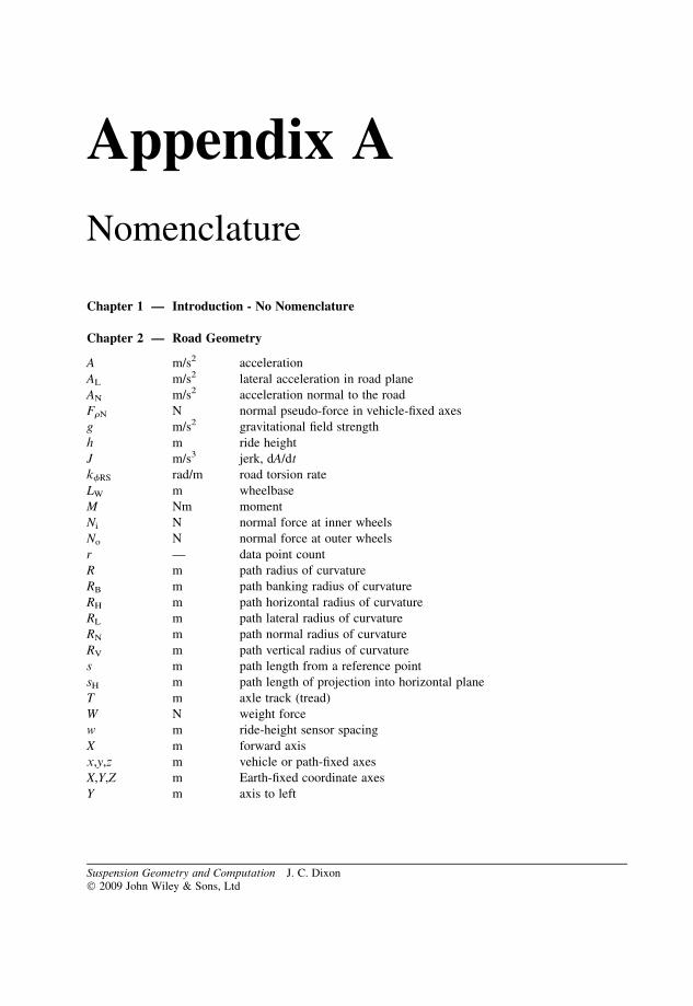
Appendix A

Nomenclature

Chapter 1 — Introduction - No Nomenclature

Chapter 2 — Road Geometry

A m/s2 acceleration

AL m/s2 lateral acceleration in road plane

AN m/s2 acceleration normal to the road

FrN N normal pseudo-force in vehicle-fixed axes

g m/s2 gravitational field strength

h m ride height

J m/s3 jerk, dA/dt

kfRS rad/m road torsion rate

LW m wheelbase

M Nm moment

Ni N normal force at inner wheels

No N normal force at outer wheels

r — data point count

R m path radius of curvature

RB m path banking radius of curvature

RH m path horizontal radius of curvature

RL m path lateral radius of curvature

RN m path normal radius of curvature

RV m path vertical radius of curvature

s m path length from a reference point

sH m path length of projection into horizontal plane

T m axle track (tread)

W N weight force

w m ride-height sensor spacing

X m forward axis

x,y,z m vehicle or path-fixed axes

X,Y,Z m Earth-fixed coordinate axes

Y m axis to left


Z m axis upwards

ZR m road altitude above datum plane

Greek

b rad vehicle attitude angle

g rad road camber angle

uLN rad wheelbase normal curvature angle

uR rad road longitudinal slope angle

k m�1 path curvature

kB m�1 path banking curvature

kH m�1 path horizontal curvature

kL m�1 path lateral curvature

kN m�1 path normal curvature

kV m�1 path vertical curvature

n rad path angle

s m lateral position from road centreline

tC m�1 s�1 car (vehicle) turn-in

tP m�2 path turn-in

tP;D m�2 driver-perceived path turn-in

fA rad axle roll angle (on tyres)

fB rad body roll angle

fR rad road lateral slope angle (bank, camber)

fS rad suspension roll angle

fSen rad roll angle of sensor reference line

fk rad angle of path curvature from horizontal

c rad vehicle heading angle

Subscripts

A axle

B body

C car

H horizontal

L lateral

N normal

P path

R road

V vertical

Chapter 3 — Road Profiles

C m cosine component amplitude

fN Hz natural frequency

fR Hz frequency of road wave at vehicle speed V.

G – gradient

H m height

kfRS rad/m road torsion

LW m wheelbase

nSR cycles/m road wave spatial frequency (see vSR)

s m path length

sH m path length in XY plane

S m sine component amplitude


T m vehicle track (tread), path spacing

TR s period of a road wave at speed V

V m/s vehicle speed

X m longitudinal position, straight path length

Z m vertical position

ZB m road banking (camber) height

ZB0 m road banking amplitude

ZL m height of left path

ZR m height of right path

ZS m road centreline height

ZS0 m road centreline amplitude

Z0 m total component of a sinusoid

Greek

u rad angle

uR rad road pitch angle

l m sinusoid wave length

lR m road wave length

f rad phase angle

fRB rad road banking angle

fRT rad road torsion angle between two axles

vR rad/s road fluctuation effective temporal frequency

vSR rad/m road fluctuation spatial frequency (see nSR)

Subscripts

B antisymmetrical (banking)

L left path

R right path

S symmetrical (centreline)

0 total amplitude (with phase angle)

Chapter 4 — Road Geometry

A m/s2 acceleration

a m front axle to centre of mass

b m rear axle to centre of mass

CC Ns/m cushion damping coefficient

CT Ns/m tyre damping coefficient total

CW Ns/m suspension damping coefficient (total)

DP — discomfort of passenger

DT — discomfort of tyre

FN N tyre normal force

g m/s2 gravity (ISO standard 9.80665m/s2)

hT m tyre vertical deflection

kf rad/m s�2 roll gradient

KC N/m cushion stiffness

KT N/m tyre vertical stiffness total

KW N/m suspension stiffness (wheel rate) total

LCP m tyre contact patch length

Nomenclature 361

mB kg vehicle body mass

mP kg passenger mass (effective on seat)

mU kg unsprung mass total

RU m tyre unloaded radius

RL m tyre loaded radius

RR m tyre rolling radius

RCE m contact patch end radius

RM — motion ratio

T m vehicle track (tread)

V m/s velocity

VX m/s longitudinal velocity

Z m vertical position

z m ride position (from static)

ZB m vehicle body vertical position

zB m vehicle body ride position

zC m cushion ride deflection (compression positive)

ZP m passenger vertical position

zP m passenger ride position

ZR m road vertical position

zS m suspension ride deflection (compression positive)

zT m tyre ride deflection (compression positive)

ZW m wheel vertical position

Greek

u rad angle

uCP rad contact patch subtended angle

fA rad axle roll angle


fBT rad body torsion angle

fR rad road bank (roll) angle

fRT rad road torsion angle


O rad/s wheel angular spin speed

Subscripts

B body (vehicle)

C cushion

f front

i inner cornering side

L left

o outer cornering side

r rear

R right

s spring

S suspension

U unsprung

W wheel

0 static


Chapter 5 — Vehicle Steering

b m kingpin offset

c m caster offset

f — a factor

fA — Ackermann factor

G — steering gear ratio

Gm — mean steering gear ratio

l — x-direction cosine

L m wheelbase, a length

Lf m front axle to centre of mass

LKP m kingpin (steer axis) length lower to upper point

Lr m rear axle to centre of mass

m — y-direction cosine

n — z-direction cosine

p m a length (Figure 5.3.4)

q m a length (Figure 5.3.4)

R m path radius to centre of mass

Rf m path radius to centre of front axle

ROT m offtracking

Rr m path radius to centre of rear axle

T m track (tread)

V m/s velocity

WKP m kingpin (steer axis) diagonal horizontal spacing

xCT m caster trail

XKC m kingpin (steer axis) caster spacing XA�XB

XKCw m kingpin (steer axis) caster spacing seen by steered wheel

yCO m caster offset

YKI m kingpin (steer axis) inclination spacing (YA� YB, left wheel)

YKIw m kingpin inclination of steered wheel


zSJ m/rad steer jacking

zSJA m/rad steer jacking of an axle

ZKI m kingpin (steer axis) vertical spacing

ZKP m kingpin height lower to upper point

Greek

a rad tyre slip angle

b rad attitude angle

g rad camber angle of road wheel

gS rad wheel camber angle due to steer

d rad steer angle of road wheel

dK rad kinematic steer angle of road wheel

dK,T rad kinematic steer angle of tractor unit

dref rad reference steer angle of road wheel

dS rad steer angle of hand wheel

d5 rad yaw angle at articulated fifth wheel

eBCas1 rad/m linear bump caster coefficient

eBCas2 rad/m2 quadratic bump caster coefficient

eSC1 — linear steer camber coefficient (deg/deg)

Nomenclature 363

eSC2 rad�1 quadratic steer camber coefficient

eSJ1 m/rad steer jacking linear coefficient

eSJ2 m/rad2 steer jacking quadratic coefficient

eSKC1 — steer kingpin caster linear coefficient (rad/rad)

eSKC2 rad�1 steer kingpin caster quadratic coefficient (rad/rad2)

eSKI1 — steer kingpin inclination linear coefficient (rad/rad)

eSKI2 rad�1 steer kingpin inclination quadratic coefficient (rad/rad2)

l rad Langensperger angle

lf0 rad Langensperger angle, front, zero speed

uB rad body pitch angle

uKC rad kingpin (steer axis) caster angle

uKC0 rad kingpin (steer axis) static straight caster angle

uKCw rad kingpin caster angle of steered wheel

uKC,R rad kingpin (steer axis) caster angle relative to the road

uKI rad kingpin (steer axis) inclination angle

uKIw rad kingpin (steer axis) inclination angle of steered wheel

uKP rad kingpin (steer axis) total angle from vertical

uStA rad steering linkage Ackermann effect angle

uStA,I rad ideal steering linkage Ackermann effect angle

uTRGE rad track rod geometry error

fSJA rad steer roll jacking of an axle

cKP rad kingpin (steer axis) sweep angle

cKPw rad kingpin (steer axis) sweep angle seen by steered wheel

Subscripts

f front

KC kingpin caster

KI kingpin inclination

KP kingpin (steer axis)

L left

L lower point of steer axis

r rear

R right

U upper point of steer axis

0 initial, static, or at zero speed

Chapter 6 — Bump and Roll Steer

a m centre of mass to front axle

b m centre of mass to rear axle

eH m rack height error

eL m track-rod length error

kRUFV N�1 variation of eRU with axle load

kRUZA m�1 variation of eRU with axle suspension bump

KA N/m axle suspension vertical stiffness

LAX m steering-arm length perpendicular to track rod

LITR m ideal track-rod length

LTR m track-rod length


zA m axle mean suspension bump deflection

zS m suspension bump deflection


Greek

dA rad axle steer angle

dA0 rad axle static steer angle

dBS rad single-wheel bump steer angle

dDBS rad axle double-bump steer angle

dRS rad axle roll steer angle

dRT rad axle roll toe-out angle

dRU rad axle roll understeer angle

dS rad driver-controlled steer angle

dT rad axle toe-out angle

dT0 rad static toe-out angle

e various suspension geometric coefficients (various units)

eBS1 rad/m single-wheel linear bump steer coefficient

eBS2 rad/m2 single-wheel quadratic bump steer coefficient

eDBS1 rad/m axle linear double-bump steer coefficient

eDBS2 rad/m2 axle quadratic double-bump steer coefficient

eRS1 — axle linear roll steer coefficient (rad/rad)

eRS2 rad�1 axle quadratic roll steer coefficient (rad/rad2)

eRT1 — linear axle roll toe coefficient (rad/rad)

eRT2 rad�1 axle quadratic roll toe coefficient(rad/rad2)

eRU1 — axle linear roll understeer coefficient (rad/rad)

eRU2 rad�1 axle quadratic roll understeer coefficient (rad/rad2)

eVHU1 rad/m vehicle linear heave understeer coefficient

eVHU2 rad/m2 vehicle quadratic heave understeer coefficient

eVPU1 — vehicle linear pitch understeer coefficient (rad./rad)

eVPU2 rad�1 vehicle quadratic pitch understeer coefficient (rad/rad2)

eVRU1 — vehicle linear roll understeer coefficient (rad/rad)

eVRU2 rad�1 vehicle quadratic roll understeer coefficient (rad/rad2)

uS rad suspension pitch angle

rA rad axle location-axis inclination angle


Subscripts

f front

L left

r rear

R right

Chapter 7 — Camber and Scrub

cy — swing centre lateral movement coefficient

cz — swing centre vertical movement coefficient

kfAfS — variation of axle roll angle with suspension roll

T m track (tread)

VCH m/s contact patch horizontal velocity

VS m/s suspension bump velocity

y m swing centre lateral coordinate

z m swing centre vertical coordinate

zB m body vertical ride position

Nomenclature 365


zW m wheel vertical ride position

Greek

a rad slip angle

b rad body attitude angle

g rad camber angle

gA rad axle camber angle

gBC rad bump camber angle

gd rad semi-difference of wheel camber angles (¼ GA)

gL rad left wheel camber angle

gm rad mean of wheel camber angles (¼ gA)gR rad right wheel camber angle

g0 rad static camber angle

G rad inclination angle

GA rad axle mean inclination angle

GARI rad axle roll inclination angle

GL rad inclination angle of left wheel

GP rad inclination angle of path (road) surface

GR rad inclination angle of right wheel

GW,L rad inclination angle of left wheel relative to the local road surface

GW,R rad inclination angle of right wheel relative to the local road surface

eARC1 — axle linear roll camber coefficient

eARC2 — axle quadratic roll camber coefficient

eARI — axle roll inclination coefficient (rad/rad)

eARI1 — axle first roll inclination coefficient (rad/rad)

eARI2 rad�1 axle second roll inclination coefficient

eBC rad/m bump camber coefficient

eBC1 rad/m linear bump camber coefficient

eBC2 rad/m2 quadratic bump camber coefficient

eBSc — local bump scrub coefficient ds/dzSeBSc1 — linear bump scrub coefficient

eBSc2 m�1 quadratic bump scrub coefficient

eBScd — local bump scrub rate coefficient

eBScd0 — initial bump scrub rate coefficient

eBScd1 m�1 linear bump scrub rate coefficient

eBScd2 m�2 quadratic bump scrub rate coefficient

uSA rad swing arm angle

fA rad axle roll angle


Subscripts

L left

R right

0 static

Chapter 8 — Roll Centres

B m lateral position of GRC in vehicle coordinates

fLT — load transfer factor


FLJ N link jacking force

FLT N suspension normal force lateral transfer (‘load transfer’)

FY N lateral force in suspension links

F1 N suspension force reacted by springs

F2 N suspension force reacted by links

g m/s2 gravitational field strength

H m height of GRC in vehicle coordinates

HCM m height of body centre of mass in vehicle coordinates

HFRC m height of FRC in vehicle coordinates

HKRC m height of KRC in vehicle coordinates

JAR — anti-roll factor

kB1 s2 linear coefficient in B(AY) [m/(m s�2)]

kB2 s4/m quadratic coefficient in B(AY) [m/(m s�2)2]

kH1 s2 linear coefficient in H(AY) [m/(m s�2)]

kH2 s4/m quadratic coefficient in H(AY) [m/(m s�2)2]

kZA s2 linear coefficient in zA(AY) [m/(m s�2)]

kfS rad.s2/m linear coefficient in fSðAYÞmB kg mass of body (sprung mass)

MFYL Nm moment of link force

MYCM Nm moment of body weight force

T m track (tread)

Y m lateral position of GRC in road coordinates

YCM m lateral position of body centre of mass in roll

YP m lateral position of body pivot point in roll

zA m axle suspension double bump (mean of two wheels)

zB m body heave

zL m suspension left bump

zR m suspension right bump

Z m height of GRC in road coordinates

ZBf m body heave after roll

Greek

e var. suspension geometric coefficient

eBSc — bump scrub coefficient in vehicle coordinates

eBScR — bump scrub coefficient in road coordinates

eBSc1 m�1 linear bump scrub coefficient

eBSc2 m�2 quadratic bump scrub coefficient

eBscd0 — bump scrub rate at zero bump

eBScd1 m�1 linear bump scrub rate variation coefficient

eBScd2 m�2 quadratic bump scrub rate variation coefficient

eB1,DB — linear variation of B in double bump

eB1,Roll m/rad linear variation of B in roll, with respect to suspension roll angle

eB1,Roll,ZB — linear variation of B in roll, with respect to wheel bump ZR (m/m)

eH1,DB — linear variation rate of GRC height in double bump, in vehicle body

coordinates

eH1,Roll m/rad linear variation of GRC height in roll

eH2,Roll m/rad2 quadratic variation of GRC height in roll

eZ1,DB — linear variation rate of GRC height in double bump, in road coordinates

uSA rad angle of swing arm


Nomenclature 367

Subscripts

L left

R right

LþR sum of left and right parts

L�R left part minus right part

L�R product of left and right parts

0 initial position, constant

1 linear, or spring part of force

2 quadratic, or link part of force

Chapter 9 — Compliance Steer

C various compliance matrix

CX,FX m/N compliance coefficient for X displacement due to FX

Cg,FY rad/N compliance camber coefficient for FY

Cg,MZ rad/Nm compliance camber coefficient for MZ

Cd,FY rad/N compliance steer coefficient for FY

Cd,MZ rad/Nm compliance steer coefficient for MZ

Cd,FX,WCH rad/N compliance steer coefficient for FX at wheel centre height

F N, Nm force–moment vector

FX N longitudinal force

FY N lateral force

FZ N normal force

kd,C rad/m.s�2 compliance steer gradient

kd,FY rad/m.s�2 compliance steer gradient due to FY

kd,MZ rad/m.s�2 compliance steer gradient due to MZ

KS N/m suspension vertical stiffness (‘wheel rate’)

KZT N/m tyre vertical stiffness

mBf kg front body mass (front sprung mass)

mBr kg rear body mass (rear sprung mass)

MD Nm driveshaft moment (torque)

MX Nm overturning moment

MY Nm pitch moment

MZ Nm yaw moment (aligning moment)

RL m wheel loaded radius

t m tyre pneumatic trail

X m, rad compliance linear and angular displacement vector

X, Y, Z m axis coordinates

XC, YC, ZC m compliance linear deflections

Greek

g rad road wheel inclination angle, camber angle

gC rad road wheel compliance inclination angle

gG rad road wheel geometric inclination angle

d rad road wheel steer angle

dC rad road wheel compliance steer angle

dG rad road wheel geometric steer angle

u rad wheel hub pitch angle

uC rad wheel hub compliance pitch angle

uG rad wheel hub geometric pitch angle


Subscripts

C compliance

D driveshaft

G geometric

X, Y, Z axis directions

Chapter 10 — Pitch Geometry

a m front axle to centre of mass

AB m/s2 braking deceleration (�Ax)

Ax m/s2 longitudinal acceleration

b m rear axle to centre of mass

F N force

FS N effective spring force

FTX N longitudinal load transfer

FV N axle vertical force

H m height of vehicle centre of mass

HS m height of sprung centre of mass

JAD — anti-dive coefficient

JAL — anti-lift coefficient

JAR — anti-rise coefficient

JAS — anti-squat coefficient

kSP Nm/rad pitch stiffness on suspension

kTP Nm/rad pitch stiffness on tyre vertical stiffness

KS N/m suspension vertical stiffness (one wheel)

Kt N/m tyre vertical stiffness (one wheel)

LAD m anti-dive pitch arm radius

LAE m anti-dive pitch arm length

LW m wheelbase

m kg vehicle mass

mS kg sprung mass

M Nm moment

MTXS Nm suspension pitch moment

MTXT Nm total longitudinal pitch moment

p — fraction of braking force at the front axle

t — fraction of tractive force at the front axle

W N weight force (mg)

zSf m front suspension bump

Greek

eBCas rad/m bump caster coefficient

uB rad pitch angle of body

uBCas rad bump caster angle

ucf rad angle of front line to wheel centre

ucr rad angle of rear line to centre

uC rad caster angle

uC0 rad static caster angle

ugf rad angle of front line to ground

ugr rad angle of rear line to ground

Nomenclature 369

uS rad suspension pitch angle

uU rad pitch angle of unsprung mass

Subscripts

BCas bump caster

c to wheel centre

C caster

f front

g to ground

i ideal

r rear

S suspension

Chapter 11 — Single-Arm Suspensions

Ca N/rad tyre cornering coefficient dFY/daCg N/rad tyre camber coefficient dFY/dgFY N tyre lateral force

HAx m height of pivot axis

HP m height of pitch centre

HS m height of swing centre

l — X direction cosine

L m a length

LA m arm length pivot axis to wheel centre

LC m pivot axis to contact patch/point

LP m pitch arm length

LS m swing arm length

m — Y direction cosine

n — Z direction cosine

RA m plan view arm length

RC m plan view length to contact point (�RA)

RL m wheel loaded radius

RP m pitch arm length, plan view

RS m swing arm length, plan view

zCP m contact patch bump

ZCP m contact patch height above datum


zW m wheel bump

ZW m wheel centre height above datum

Greek

g rad road wheel camber angle

d rad road wheel steer angle



eBKC1 rad/m linear bump kingpin caster angle coefficient

eBKC2 rad/m2 quadratic bump kingpin caster angle coefficient

eBKI1 rad/m linear bump kingpin inclination angle coefficient

eBKI2 rad/m2 quadratic bump kingpin inclination angle coefficient

eBScd0,T — total bump scrub rate coefficient


eBScd0,X — bump scrub rate coefficient, X component

eBScd0,Y — bump scrub rate coefficient, Y component

eBS1 rad/m linear bump steer coefficient

eBS2 rad/m2 quadratic bump steer coefficient

uA rad arm angle about axis, wheel end up

uAx rad pivot axis yaw angle (p/2�cAx)

uC rad angle of line pivot axis to contact patch/point

uK rad kingpin total angle from vertical

uKC rad kingpin inclination angle

fAx rad pivot axis angle (out of horizontal)

cAx rad pivot axis sweep angle

cK rad kingpin sweep angle

Subscripts

0 initial, zero bump, conditions

Superscripts

u; v circumflex cap indicates unit vectors

Chapter 12 — Double-Arm Suspensions

fBJH — HBJS/HBJD, sum/difference height factor

HBJD m HBJU�HBJL, height difference

HBJL m static height of lower outer ball joint

HBJM m HBJS/2¼ (HBJUþHBJL)/2, mean height

HBJS m HBJUþHBJL, height sum

HBJU m static height of upper outer ball joint

HP m height of pitch centre

HS m height of swing centre

L m length

LP m length of pitch arm

LS m length of swing arm

LXL m length of equivalent lower longitudinal arm

LXU m length of equivalent upper longitudinal arm

LYL m length of equivalent lower lateral arm

LYU m length of equivalent upper lateral arm

R m arc radius

RP m pitch arm radius

RS m swing arm radius

s m scrub

S m�1 shortness, reciprocal of length

SXD m�1 longitudinal shortness difference SXU� SXLSXL m�1 shortness of equivalent lower longitudinal arm

SXS m�1 longitudinal shortness sum SXUþ SXLSXU m�1 shortness of equivalent upper longitudinal arm

SYD m�1 lateral shortness difference SYU� SYLSYL m�1 shortness of equivalent lower lateral arm

SYS m�1 lateral shortness sum SYUþ SYLSYU m�1 shortness of equivalent upper lateral arm

u m local coordinate

Nomenclature 371

v m local coordinate

V m/s velocity

w m local coordinate

y m lateral coordinate

yL m lateral displacement of lower ball joint

yU m lateral displacement of upper ball joint

z m vertical coordinate


Greek

gB rad bump camber angle

eBcas1 rad/m linear bump caster coefficient

eBcas2 rad/m2 quadratic bump caster coefficient



eBScd — local bump scrub rate coefficient (at zS) (m/m)

eBScd0,X — longitudinal bump scrub rate static (m/m)

eBScd1,X m�1 longitudinal bump scrub rate variation (m/m2)

eBScd0,Y — lateral bump scrub rate static (m/m)

eBScd1,Y m�1 lateral bump scrub rate variation (m/m2)

eBSc1 — linear lateral bump scrub coefficient (m/m)

eBSc2 m�1 quadratic lateral bump scrub coefficient (m/m2)

u rad angle

uSL rad angle of strut slider from vertical

uXD rad uXU� uXLuXL rad angle of equivalent lower longitudinal arm

uXS rad uXUþ uXLuXSL rad side-view angle of strut slider from vertical

uXU rad angle of equivalent upper longitudinal arm

uYD rad uYU� uYLuYL rad angle of equivalent lower lateral arm

uYS rad uYUþ uYLuYSL rad front-view angle of strut slider from vertical

uYU rad angle of equivalent upper lateral arm

f rad angle

c rad angle

v rad/s angular velocity

O rad/s angular velocity

Subscripts

0 Static value (zero suspension bump)

Chapter 13 — Rigid Axles

CI,J var link space sensitivity matrix

E m link space length errors

H m roll centre height

HA m axle vertical spacing of links

l, m, n — direction cosines (e.g. of a link)

LAx m axle length between wheel centres

LT13PV m length in plan view between triangle points 1 and 3


R m a radius


x, y, z m coordinate system

x m longitudinal coordinate (forwards)

X m surge, and a general variable

y m lateral coordinate (to the left)

Y m sway

z m vertical coordinate (upwards)

Z m heave

zAS m axle suspension heave (symmetrical double bump)

zSBL m suspension bump left

zSBR m suspension bump right

Greek

d rad steer angle (axle yaw angle)

eAHP rad/m axle heave pitch coefficient

eAHS rad/m axle heave steer coefficient

eAHSc,X — axle heave scrub coefficient, longitudinal

eAHSc,Y — axle heave scrub coefficient, lateral

eAHX — axle heave surge coefficient

eAHY — axle heave sway coefficient

eARP — axle roll pitch coefficient

eARS — axle roll steer coefficient

eARSc,X m/rad axle roll scrub coefficient, longitudinal

eARSc,Y m/rad axle roll scrub coefficient, lateral

eARX m/rad axle roll surge coefficient

eARY m/rad axle roll sway coefficient

u rad pitch/caster angle, angle generally

f rad roll angle

fA rad axle roll angle (on tyres)


fS rad axle suspension roll

Chapter 14 — Installation Ratios

CD Ns/m damper coefficient

CSD Ns/m effective damper coefficient seen at suspension

e m offset

F N force

FD N force at damper

FK N compression force at spring

Fm N force at point mass

fR – rising rate factor

FSK N spring force active at suspension

KK N/m spring stiffness

KSK N/m effective spring stiffness seen at suspension

KW N/m total spring/bush wheel rate (mainly KSK)

l m rocker arm length

l — X-direction cosine

lWP m length from wheel centre to pivot axis (in plan)

L m length

Nomenclature 373

LK m spring length

m — Y-direction cosine

n — damper characteristic exponent

n — Z-direction cosine

R — motion ratio

R0 m�1 motion ratio variation dR/dzSRA/B — motion ratio of item A relative to item B

RAPH — motion ratio for pitch in heave

RD — damper motion ratio dxD/dzSRDC — damper coefficient ratio

RDf m/rad damper velocity ratio in roll

RK — spring motion ratio dxK/dzSRm — motion ratio of a point mass

RR — rocker motion ratio

RRL — rocker arm length motion ratio

RRc — rod angle motion ratio

RRc0 — rod angle motion ratio at u¼ 0

t s time

T m axle track

u m/s X -velocity component

v m/s Y-velocity component

V m/s velocity

VA m/s velocity of point A

(VX, VY, VZ) m/s velocity coordinates

VD m/s damper compression velocity

VK m/s spring compression velocity

VP m/s pushrod velocity

VS m/s suspension bump velocity

w m/s Z-velocity component

x m displacement

xD m damper compression from static

xK m spring compression from static

xP m pushrod displacement from static

(X, Y, Z) m coordinates

zB m body displacement

zD m damper compression

zS m suspension displacement in bump

zW m wheel displacement

Greek

aD rad damper out-of-plane angle

aK rad spring out-of-plane angle

g rad wheel camber angle

eAPH rad/m axle pitch/heave coefficient

eBC rad/m bump camber coefficient

eBScd – local bump scrub rate coefficient

eDBScd0 – linear bump scrub rate coefficient (m/m)

eDBScd1 m�1 quadratic bump scrub rate coefficient (m/m2)

uR rad rocker position angle

uRD rad rocker deviation angle

fR rad rocker included angle


c rad rocker rod offset angle from tangent

cZ rad c at static ride height (zero bump)

v rad/s angular speed

vR rad/s rocker angular velocity

Subscripts

D damper

K spring

m mass (point mass)

P pushrod

S suspension

W wheel

z static (zero) ride height

1 input

2 output

Chapter 15 — Computational Geometry in Three Dimensions

In some cases the units may vary. This depends on the type of problem being solved (e.g. a position

problem or a velocity diagram problem).

Variables are in italics, vectors are in bold italics, and magnitudes of vectors are in non-bold italics.

a1,. . .,a5 various various constant values

A m position or displacement vector

A m magnitude of Aa, b, c m side lengths of triangle

A, B, C rad angles in a triangle

b1, b2 various constant values

B m position or displacement vector

B m magnitude of Bc1,. . .,c5 various various constant values

d various determinant value, divisor

D m position or displacement vector

D m magnitude of Df — position factor (e.g. on a line)

f1, f2, f3 — position factors in a triangle

i; j; k — unit vectors along (x, y, z)

L m length

l, m, n — direction cosines

L, M, N — direction numbers

N m vector normal to a plane

N m magnitude of Np m constant in plane equation

P various vector cross product

P various vector dot product, or cross product magnitude

R m radius of circle or sphere

s m displacement along a line

u, v, w m local coordinate position

u, v, w m/s velocity components

u; v; w — unit vectors in local coordinates

V m/s velocity vector

Nomenclature 375

V m/s velocity magnitude

VN m/s velocity component normal to a plane

VT m/s velocity component tangential

x, y, z m coordinate position

zHP m height of horizontal plane

Greek

a, b, g rad direction angles

u rad angle (e.g. between two vectors)

O rad/s angular velocity

Chapter 16 — Programming Considerations

f — interpolation factor

l, m, n — direction cosines or numbers

p m a constant

u, v, w m coordinates

x, y, z m coordinates

Chapter 17 — Iteration

a — 1� r

a, b, c, d — Muller’s method coefficients

A — asymptotic error constant

C — a constant

dK — difference between successive changes

dx — a small change in x

D — simultaneous equation divisor

e — an error value

eK — error at Kth iteration

f — a function f (x)

f 0 — first derivative of f

f 00 — second derivative of f

g — f f 00=2f 02

m — gradient (e.g. numerical)

p — root multiplicity factor

P — order of convergence

r — sequential error ratio

R — remainder

w — iteration ‘acceleration’ factor

x — a variable

xITER — basic proposed new value by iteration

xK — value of x after Kth iteration

y — a variable y(x)

z — possibly complex variable

ZLBJ m height of lower ball joint

ZSB m suspension bump position

Greek

D — a change in a variable

————— // —————


Appendix B

Units

This book is, of course, in SI units throughout, but variations of Imperial (‘English’) units are still in

everyday engineering use in the USA, so the conversion factors in Table B.1 may be useful. Note that lbm

denotes poundmass, lbf denotes pound force (theweight force that acts on one poundmass due to standard

gravity), kg denotes kilogram mass of course, whilst kgf denotes a ‘kilogram force’, the weight of 1 kg

mass in standard gravity. The kgf is sometimes denoted the kp, the kilopond, which is in common use in

Continental Europe. This must not be confused with the kip, a US unit of 1000 lb. The force units kgf and

kp are not true SI, in which forces are always in newtons. The pound mass is 0.453592370 kg (exact by

definition).

In basic geometry, the only measures are those of length and angle. Even here, true world standardisa-

tion has not been achieved, with the inch (25.400mm exactly by definition in the UK and US since the

1960s) still being used in the US. The international spelling of the length unit ismetre, accepted in the UK

and the rest of theworld except for the US andGermany, where it is speltmeter. In international English, a

meter is a measuring device. The number 25.4 is only moderately round, and one can look forward, once

the now only ‘US’ inch eventually dies out, to the introduction of a convenient and useful metric inch of

exactly 25mm.

In the context of suspensions, the length unit of the decimetre is useful, denoted dm, this being exactly

0.1m by definition, 100mmand 10 cm, approximately 4US inches. Coefficients such as linear bump steer

are conveniently expressed in degrees per decimetre (�/dm), with �/dm2 for quadratic bump steer. One

decimetre is a realistic large displacement for a suspension, so in these units the relative magnitude of the

coefficients is significant.

In angularmeasure, the fundamental unit is the radian (about 57.29578 degrees, exactly 180/p degrees).This angular unit is a great mystery to non-mathematicians, but makes a great deal of sense once one

appreciates its role in geometry and computation, or, indeed, in the relationship between engine torque and

energy per revolution, or power. Physically, it is the angle for which the arc length equals the radius. For

human consumption, the degree is generally preferred, or the complete revolution. In France, as an effect

of the political revolution of circa 1795, the gradian is often used, this being by definition one hundredth of

a right angle, being exactly 0.9 degrees. The sexagesimal base (the very ancient base 60) systemof angular

measure, with 60 angular seconds in one angular minute and 60 angular minutes in one degree is still used

by astronomers, but in general science and engineering it is now common, and certainly easier, to use

decimal degrees.

The main angular conversions needed are therefore between radians and degrees, and some

computer languages provide this facility by intrinsic routines, e.g. rads(angdeg) and degs(angrad).


Basic usually has RAD and DEG. Of course, these are only multiplications by the appropriate constant of

180/p or p/180.The correct use of capital letters in units is essential. Consider, for example, the possible errors in

incorrect use of kg, Kg, KG and kG, which would correctly mean kilogram, kelvin gram, kelvin gauss and

kilogauss, although the gauss is not SI.

————— // —————

Table B.1 Conversion factors

Length (SI m, metre):

1 inch¼ 0.025400m (exact by definition)

1 foot¼ 0.304800m (exact)

1m¼ 39.37008 inch (approximate)

Angle (SI rad, radian)

1 rad¼ 1/2p revolutions (exact)

1 rad¼ 180/p degrees (exact)

1 rad¼ 57.29578 deg

1 deg¼ 17.4533 mrad

1 rev¼ 360.000 deg (exact)

1 rev¼ 2p rad (exact)

1 grad¼ 1/400 rev (exact)

1 deg¼ 60min (angular minutes, exact)

1 min¼ 60 sec (angular seconds, exact)

Mass (SI kg):

1 lbm¼ 0.453592370 kg (exact, definition)

1 kg¼ 2.204622622 lbm (approximate)


Appendix C

Greek Alphabet

Lower case

Name Letter Main applications

alpha a slip angle

beta b attitude angle

gamma g camber angle

delta d steer angles

epsilon e geometric coefficients

zeta z —

eta h compliance coefficients

theta u pitch angle, angles

iota i —

kappa k path curvature

lambda l angles, Langensperger angle

mu m —

nu n path angle

xi j —

omicron o —

pi p geometric constant

rho r density, angles

sigma s —

tau t path turn-in

upsilon y —

phi f roll angles

chi x —

psi c heading angle

omega v angular velocity


(continued)

Upper case

Name Letter Main applications

alpha A —

beta B —

gamma G inclination angle

delta D non-small increments

epsilon E —

zeta Z —

eta H —

theta Q angles

iota I —

kappa K —

lambda L angles

mu M —

nu N —

xi X —

omicron O —

pi P —

rho P —

sigma S mathematical summation

tau T —

upsilon Y —

phi F angles

chi X —

psi C angles

omega O angular velocity

Many of the upper case letters are the same as the usual Latin alphabet of English, so do not arise in

mathematical symbols.

————— // —————


Appendix D

Quaternions for Engineers

D.1 Introduction

A quaternion is a group of four numbers (hence the name quat-), for example (a, b, c, d). Early work on

the properties of such four-number groups was done by Euler, but the real invention of quaternions was by

the prominent Irish mathematician Sir William R. Hamilton in 1843, who established the rotational

properties and the three imaginary numbers involved.

In particular, a quaternion is a scalar number a with a three-dimensional vector (b, c, d). There are

simple rules for addition,multiplication and so on.Quaternions can be used for efficient calculations of the

position of a rotated solid body in space, for example aircraft and space vehicles. Multiplication of

quaternions corresponds to successive rotations about possibly different axes, so they are intimately

related to the nature of three-dimensional space. This involves the use of three distinct square roots of�1,

so quaternions are an important generalisation of the usual two-dimensional complex numbers.

Quaternion addition and subtraction are simply performed term by term. Multiplication is more

complicated, being performed across all combinations of terms, with rules for the various vector products.

Division is by multiplication of a reciprocal.

The theory of quaternions was described by Hamilton as the theory of lines in space, and as the theory

of vector quotients. A quaternion converts one vector (line) into another by multiplication. Division and

reciprocation of quaternions is also required.

D.2 History

There is a saying that ‘Anything is more fun if you shouldn’t be doing it’. We are fascinated by the taboo.

The Catholic church used to have a long list of forbidden books, a list that became unofficial in the 1950s.

Many religious people would still never consider owning a book for fear of reprisals. There are religious

people who would destroy all books totally, perhaps short of the Bible in Latin. Haters of mathematics

have a special fear and loathing of complex numbers, and of quaternions in particular. Thesemathematical

devices are used, inter alia, to calculate rotations, which is the source of the fear.

Six hundred years ago, the official religious dogma was that the Earth was fixed, and was the centre of

the universe, and the world was largely a theocracy. Science showed that this was false – the Earth is in

orbit around the Sun (giving the year) and revolves on its own axis (the day), despite fierce opposition from

the church (persecution of Galileo: ‘It moves nonetheless’). The Earth has combined rotations. The Sun is

a non-special star in a non-special galaxy. This severely undermined claims that human beings are central

to the universe. Hence, the hatred of ‘rotations’. Also, the theocracy was threatened by Science, so there

was fear of ‘revolutions’, which would deny religious power, particularly a fear of combined revolutions.


The hatred of Science and books in some religions contrasts interestingly with the respect accorded to

these in others, such as Islam, Hinduism, Buddhism and, of course, by non-believers.

The application of quaternions to solid body rotation is alone enough to justify its inclusion in

undergraduate mechanics texts. Its absence therefrom, and the general dearth of material, is very

interesting itself. The suppression of quaternions has made them a cause c�el�ebre with the inevitable

attraction of the ‘forbidden’. Quaternions are also applied in subatomic physics. The correspondence

between the quaternion and four-dimensional space-time is itself fascinating.

In view of the above historical vignette, and bearing in mind the fact that the Spanish mathematician

Valmes was burned to death at the stake by the Inquisition for solving a quartic equation, let us, with a

frisson of fear and excitement, consider these dangerous quaternions, these ‘agents of revolution’. In

comparison with the apparent dramatic political importance attending them, the simple mathematical

reality is mundane indeed. It is hard to imagine anything more innocuous.

D.3 Position in Space

The general position of a body in three-dimensional space requires specification of one particular point of

the body, usually the centre of mass, in fixed coordinates (X, Y, Z), and the body’s angular position. The

rotational position is specified by rotations in a coordinate system centred at the body reference point.

Often theEuler angles are used,which are three successive rotations about, in turn, thevertical axis (giving

a heading angle), the body lateral axis (giving a pitch angle), and finally the body longitudinal axis (giving

a roll angle). However, Euler’s theorem of rotation states that any angular position of a body, however

actually reached, may be reached by a single rotation about some axis, generally inclined. Thismeans that

the rotation can be given an axis-and-angle representation, with the axis defined by direction cosines. This

is a representation in terms of four numbers, these being one scalar, the angle u, and a three-dimensional

axis vector: (u, l, m, n). Quaternions are not far from this, but modified for convenient calculation.

For an object with an initial position represented by a quaternionP1, when it is rotated to a new position

that new position is given by P2¼QCP1Q, that is, premultiplication by the conjugate QC and post-

multiplication by the quaternion Q.

D.4 Quaternion Representations

Aquaternion is a four-part number, being one part scalar and one part three-dimensional vector. Thevector

part is also known as the imaginary part. According to the job in hand, the best representationmay vary. As

a four part number it is simply

Q ¼ ða; b; c; dÞIf the vector is, as usual, directed in normal space, then the (x, y, z) axes have corresponding unit vectors

(i; j; k) and the quaternion is conveniently written as

Q ¼ q0 þ qxiþ qyjþ qzk

The Euclidean length is

LQ ¼ffiffiffiffiffiffiffiffiffiffiffiffiffiffiffiffiffiffiffiffiffiffiffiffiffiffiffiffiffiffiffiffiffiffiq20 þ q2x þ q2y þ q2z

q

A unit quaternion, having a total Euclidean length of 1, may be written in terms of its unit direction

vector as

Q ¼ cosfþ u sinf

More generally, for a quaternion of length LQ,

Q ¼ LQðcosfþ u sinfÞ


D.5 Conjugates

The conjugate of a quaternion (like the usual diernion complex number) requires the negation of the vector

(imaginary) part, so for

Q ¼ ða; b; c; dÞ

the conjugate is simply

QC ¼ ða;�b;�c;�dÞSome other useful conjugate relationships are

ðACÞC ¼ A

ðAþBÞC ¼ AC þBC

ðABÞC ¼ BCAC

with a change of order occurring in the last equation. This last relationship is used in combined rotations.

D.6 Addition and Subtraction

Addition and subtraction of quaternions is simply performed by separate addition of the four component

parts.

D.7 Multiplication

Quaternion multiplication is associative, which means that

Q1Q2Q3 ¼ ðQ1Q2ÞQ3 ¼ Q1ðQ2Q3Þ

so the rotated position quaternion P2¼QCP1Q can be calculated as (QCP1)Q or as QC(P1Q) with correctresults. Quaternion multiplication is also distributive, so

Q1ðQ2 þQ3Þ ¼ Q1Q2 þQ1Q3

The actual quaternion multiplication is performed term by term. In general,

P ¼ pþ pxiþ pyjþ pzk ¼ pþPv

Q ¼ qþ qxiþ qyjþ qzk ¼ qþQv

By reducing the products, such as i j to k, and i2to�1 (detailed later), and collecting terms, then R¼PQ

may be expressed in its components as

R ¼ rþ rxiþ ryjþ rzk

with

r ¼ pq�ðpxqx þ pyqy þ pzqzÞrx ¼ pqx þ qpx þ pyqz�pzqy

ry ¼ pqy þ qpy�pxqz þ pzqx

rz ¼ pqz þ qpz þ pxqy�pyqx

Quaternions for Engineers 383

This may be expressed conveniently in terms of the scalar and vector parts as

PQ ¼ ðpq� Pv �QvÞþ pQv þ qPv þPv �Qv

where the vector parts Pv andQv behave as conventional vectors, with a dot product on the left and a cross

product on the right. This type of quaternion product is known as the Grassman product. There are other

types of product, not relevant to rotations. The quaternion product is, then, effectively the cross product

minus the dot product.

The final vector cross product is the standard determinant

P�Q ¼i j kpx py pzqx qy qz

�� ¼ iðpyqz � pzqyÞ � jðpxqz � pzqxÞþ kðpxqy � pyqxÞ

The point position quaternion P2 resulting from the calculation should be a true position quaternion, with

zero as its scalar part. This can be demonstrated to be algebraically correct, but may be numerically

imperfect.

To obtain the quaternionmultiplication result requires consideration ofmultiplication of the component

parts with their direction unit vectors, which has a somewhat mysterious quality (see Table D.1), as with

planar complex numbers.

Table D.1 Multiplication tables

For ab use a in the left column and b in the top row. Pre- or postmultiplication by 1 always gives the same

vector.

Unit vectors, dot product

i j ki 1 0 0

j 0 1 0

k 0 0 1

Unit vectors, cross product

i j ki 0 k �j

j �k 0 i

k j �i 0

Planar complex numbers

i

i �1

Quaternions

i j ki �1 k �j

j �k �1 i

k j �i �1

This is the vector cross product minus the vector dot product. For quaternions, also note that

i2 ¼ j2 ¼ k2 ¼ i j k ¼ �1

i j ¼ �j i ¼ k

j k ¼ �k j ¼ i

k i ¼ �i k ¼ j


Here, the mystery is that in considering the direction of the axis of rotation, and for the positions of

points, the i, j and k are taken to be unit vectors. However, in the multiplication table they behave as three

distinct square roots ofminus one. The vector cross product i� i is zero, but, for quaternionmultiplication

as for planar complex numbers, i� i is�1. This means that the negated dot product appears in the scalar

part of the result quaternion. There are therefore three multiplication results for self-products of unit

vectors, the dot product 1, the vector cross product zero and the quaternion product�1. This applies to any

general unit vector, not just to axis-aligned unit vectors.

The quaternion multiplication property that i2 ¼ �1, j

2 ¼ �1 and k2 ¼ �1 shows that a quaternion

is a generalised form of a complex number in which there are three distinct square roots of�1, namely i, j

and k, about independent axes. This is directly related to the fact that in three-dimensional space there are

three independent rotations, that is, three ways to select a pair of the three axes for a rotation.

D.8 Reciprocals

The reciprocal or inverse of a quaternion is given by

Q�1 ¼ QC

L2Q

where LQ is the Euclidean length of Q, defined earlier, with

QQ�1 ¼ Q�1Q ¼ ð1; 0; 0; 0ÞThis is also the accepted method for obtaining the reciprocal of a complex number. In this special case

of the reciprocals the multiplication is commutative, QQ�1¼Q�1Q.

D.9 Division

Quaternion division is, like multiplication, non-commutative, and is performed by multiplication by a

reciprocal. The expression

Q ¼ Q1

Q2

is ambiguous, and could mean

Q ¼ Q1

1

Q2

or Q ¼ 1

Q2

Q1

which will not, in general, have the same value. The correct one to use depends on the problem in hand.

The reciprocal may be found as shown earlier, so the quotient is either

Q ¼ Q1

1

Q2

¼ Q1QC2

L2Q2

or

Q ¼ 1

Q2

Q1 ¼QC

2Q1

L2Q2


D.10 Powers and Roots

Using the axis unit vector notation, the square of Q is

QQ ¼ L2ðcos2fþ 2u sinf cosfþð�1Þsin2fÞ

where uu¼�1, showing how the quaternion self-multiplication of a unit vector must be u2 ¼�1 to give

the cos 2f¼ cos2f� sin2f:

Q2 ¼ L2ðcos 2f�sin 2fþ uð2 sinf cosfÞÞ¼ L2ðcos 2fþ u sin 2fÞ

which is squaring of the length and doubling of the argument (angle), exactly as for a diernion complex

number, and correspondingly for the nth power:

QN ¼ LNðcos Nfþ u sin NfÞNote that the direction of the axis vector u is unchanged.

Correspondingly, the square root of the quaternion Q is

ffiffiffiffiQ

p¼

ffiffiffiL

pcos 1

2fþ u sin 1

2f

� �

and correspondingly for the nth root:

ffiffiffiffiQN

p¼

ffiffiffiffiffiL

Np

cosðf=NÞð þ u sinðf=NÞÞHowever, multiplication is not conveniently achieved by this means because in general u1 6¼ u2 (unlikecomplex numbers).

D.11 Interpolation

In the simulation of solid body motions, as used in flight training simulators and computer games, it is

often desired to interpolate smoothly between two angular positions of a body, If these angular positions

are specified by Q1 and Q2, it is required to find the intermediate transform quaternion Q where

QQ1 ¼ Q2

so

Q ¼ Q2Q�11

Q ¼ Q2QC1

L2Q1

It is then easy to interpolate for intermediate positions by fractioning the angle of the quaternion Q.

D.12 Point Position Quaternions (Vector Quaternions)

For the purposes of basic physics and engineering, it is convenient to think in terms of two types of

quaternion. After the body reference point is specified, a local set of axes centred there is considered,

parallel to themainEarth-fixed axes.Anypoint in the body has a position in the local axes, represented by a

position vector and a corresponding local point position quaternion. The other particular type of


quaternion is the rotation quaternion itself. These two types are just special cases. For a point position

vector in local axes (x, y, z) the corresponding point position quaternion is

P ¼ ð0; x; y; zÞAll point position quaternions have a zero first part. This also illustrates how a quaternion is a combination

of a scalar part, the first number, and a three-dimensional vector part, the last three numbers, analogous to

time and space. Using the usual unit vectors i; j; k, along axes x, y, and z, the point position quaternion

may be expressed as

P ¼ 0þ x iþ y jþ z k

This use of a point position quaternion touches upon the use of homogeneous coordinates, which in three

dimensions are (a, x, y, z) or (x, y, z, a), where the extra member a is used to scale the basic point position

(x, y, z) to handle points at infinity without loss of direction.

D.13 Standard Rotation Quaternions

Consider now rotation by angle u (radians) with, for convenience,f¼ u/2, positive right-handed about anaxis through the origin defined by direction cosines (l, m, n). The corresponding standard rotation

quaternion is

Q ¼ ðcosf; l sinf;m sinf; n sinfÞ

also expressible in terms of unit vectors as

Q ¼ cosfþðl sinfÞiþðm sinfÞ jþðn sinfÞkThe vector part of the standard rotation quaternion points along the axis of rotation, and has a length of sin

f¼ sin(u/2).The Euclidean length of a standard rotation quaternion is

LQ ¼ ffip ðcos2fþ sin2fðl2 þm2 þ n2ÞÞ ¼ ffip ðcos2fþ sin2fÞ ¼ 1

This unit Euclidean length is a useful feature of a standard rotation quaternion, unlike a position

quaternion which can be any length but must have a zero first (scalar) part. Hence, the scalar part of a

standard rotation quaternion bulks up the Euclidean length to unity. This eliminates any scaling effect.

D.14 Angular Position

Given an initial position, then the angular position of a body at any other time may be represented by the

appropriate rotation quaternion from that reference state. This angular position quaternion is the product

of all the angular movement quaternions in the intervening time, taken in the correct sequence.

For a rotation through angle u¼ 2f, the rotation quaternion and its conjugate are

Q ¼ ðcosf; l sinf;m sinf; n sinfÞQC ¼ ðcosf;�l sinf;�m sinf;�n sinfÞ

which is the same as negating the angle.

When the rotation of the body about the axis occurs, any point P1 with angular position quaternion P1

moves to position P2, with angular position quaternion

P2 ¼ QCP1Q


giving the desired values for the new position. Because quaternionmultiplication is not commutative, it is

essential that the premultiplication be by the conjugate, not the other way round. If they are reversed, it is

as if the angle were negated. This would be equivalent to rotating the coordinate system with the body

stationary, rather than moving the body itself.

In the above equation is a clue to the use of only half of the physical rotation angle in each quaternion. It

is useful to think that postmultiplication moves the body by half of the angle, but with some side effects.

Premultiplication byQwouldmove it in the other direction, so the angle is negated by using the conjugate.

The combination of pre- and postmultiplication eliminates the side effects, leaving only the required

angular movement.

The angular position calculation requires two quaternionmultiplications.Multiplication of quaternions

is non-commutative, meaning that Q1Q2 does not in general have the same value as Q2Q1. This aspect of

some operators is well understood nowadays, but was highly ‘revolutionary’ in 1843. In effect it is a

mathematical consequence of the physical fact that two rotations about different axes have different final

results if done in a different order.

D.15 Reversed Axis

In three-dimensional geometry, if the direction of the rotation axis is reversed and the angle is negated then

the physical result of the rotation must be the same. For a quaternion, this is

Q1 ¼ cos fþ u sin f

Q2 ¼ cos fþð�uÞsinð�fÞ¼ cos fþð�uÞð�sin fÞ¼ cos fþ sin f

so the quaternion is the same, as it should be.

D.16 Special Rotation Cases

A rotation quaternion with a rotation angle of 90� has cos 45� and sin 45�, and does not look special.

At 180� rotation, it has cos 90� and sin 90�, and the scalar part becomes zero, Q being simply

Q ¼ ð0; l;m; nÞA rotation of �180�, which is 180� in the other direction, is

Q ¼ ð0;�l;�m;�nÞwhich has the same final result.

A zero rotation, leaving the object in its original position, has cos 0� (¼þ1) and sin 0� (¼ 0) with

rotation quaternion

Q ¼ ð1; 0; 0; 0ÞA complete 360� rotation, or�360�, leaving the object in its original position, has cos 180� (¼�1) and

sine 180� (¼ 0) with rotation quaternion

Q ¼ ð�1; 0; 0; 0Þ

If this is applied twice, 720� rotation, then the original position is achieved once again. The product of thetwo 360� rotation quaternions is (1, 0, 0, 0), the other rotation quaternion that leaves the body in its originalposition.


The need for two 360� rotations to restore the quaternion to its original state is significant. It has beenheld to imply something about the nature of space-time, and is important in the description of some

subatomic particles which seem to have this same property.

D.17 Negation

If a rotation quaternion is fully negated, Q2¼�Q1, its effect is unchanged. Solving for the angle f from

the quaternion components shows that it is changed by 180�. The actual rotation angle is changed by twicethat, 360�, a complete rotation, so the results are the same. This means that there are two quaternions

representing any one rotation. When a negative scalar part occurs, the entire quaternion may therefore be

negated, to produce a ‘reduced’ quaternion of the same rotational properties but with a positive scalar part.

D.18 Non-Unit Rotations

The foregoing explanation of rotation was couched in terms of standard rotation quaternions, also known

as unit quaternions, with Euclidean length 1. Strictly, this is not necessary. If P1 is rotated by unit

quaternion Q to P2 then

P2 ¼ QCP1Q

IfQ is multiplied by a scalar constant A, then R¼AQ does not have unit Euclidean length, and the above

equation no longer holds – a scaling with factor A2 occurs. However, it is still correct that

P2 ¼ R�1P1R ¼ ðAQÞ�1P1ðAQÞ

using premultiplication by the reciprocal instead of the conjugate. The factor A then increases the

intermediate product but this scaling is corrected by the second multiplication. The precalculation ofR�1

requires

R�1 ¼ RC

L2R

In the special case of unit quaternions, with L¼ 1,R�1¼RC, the reciprocal equals the conjugate, making

for amore efficient calculation. For this reason, rotations are, in practice, represented by normalised (unit)

quaternions.

D.19 Sequential Rotations

Two rotations in succession,Q1 andQ2 in that order, have a total resultQ. Point position P1 goes viaQ1 into

P2 and then via Q2 into point position P3 with quaternion P3:

P3 ¼ QC2 QC

1P1Q1

� �Q2

The multiplication is associative, so

P3 ¼ QC2Q

C1

� �P1 Q1Q2ð Þ

It is a property of the conjugates that

QC2Q

C1 ¼ Q1Q2ð ÞC


with the order changing, so

P3 ¼ Q1Q2ð ÞCP1 Q1Q2ð Þ

and the total effect is given simply by

Q ¼ Q1Q2

taken in the order in which they occur. This applies to any succession of rotations:

Q ¼ Q1Q2 � � �QN

A long sequence of such calculations can introduce cumulative numerical errors. With a matrix

representation of rotation this can be difficult to correct, because the rotation matrix has a complex

relationship between its parts.A rotation quaternion is easily renormalised because the one specification to

be met by a standard rotation quaternion is that it have a Euclidean length of exactly 1, which is a helpful

feature in numerical work.

D.20 Relationship with Complex Numbers

In two dimensions, in the complex plane, rotation through an angle umay be performed bymultiplying by

the complex number z¼ (cos u þ i sin u). In two dimensions, there is only one possible rotation, which is

an interchange between x and ywithout change of length. In three dimensions, three possible independent

rotations are possible. Considering axis-aligned rotations, these are exchangingxwith y, ywith z or zwith

x, so a quaternion has three independent rotations, and so three roots of�1 for three-dimensional rotations

instead of the diernion complex number single root i for two-dimensional rotations.

In two-dimensional geometry, multiplying by i¼H�1 is a 90� turn to the left, about the virtual z axis.Two such turns, which is a multiplication by i2¼�1, gives a 180� turn, which is a full reversal (þ 1 into

�1). Another square root of �1 is �i. This is a 90� turn in the opposite direction, to the right. Two suchturns equals �180�, which is the same position as þ 180�.In complex numbers, rotation (e.g. multiplication) is supposed to be about a virtual axis perpendicular

to the plane (1, i), but uses equations for rotation about an i axis. However, in three dimensions, rotations

about the i axis are in the (j, k) plane. It happens that i� j¼ k and i� k¼�j. In two dimensions, we use

i� 1¼ i and i� i¼�1, which is two-dimensional complex numbers are really in the (j, k) plane, not the

(1, i) plane, but the renaming of j as 1 and k as i happens to work.

D.21 Infinitesimal Rotations

For an infinitesimal rotation, the angles u andf themselves are infinitesimals and all higher orders such as

f2 can be neglected. Then sinf�f and cosf� 1, so

Q ¼ ð1; lf;mf; nfÞ

Table D.2 Comparison of i in two and three dimensions

2D 3D

(j, k) plane (1, i) plane

i� j¼ k i� 1¼ i

i� k¼�j i� i¼�1

i2 ¼ �j

j¼ �1 i2 ¼ �1

1¼ �1


Considering two such infinitesimal rotations, Q1 and Q2, the total effect is Q¼Q1Q2 which, by

multiplying out and eliminating higher-order infinitesimals, gives

Q ¼ ð1; lðf1 þ f2Þ;mðf1 þ f2Þ; nðf1 þ f2ÞÞ

which is why angular velocities, unlike angular positions, behave as simple vectors.

D.22 Vector Quaternions

For pure vector quaternions (zero scalar part)

QV1QV2 ¼ �QV1 �QV2 þQV1�QV2

QV2QV1 ¼ �QV1 �QV2 �QV1�QV2

where the first term is a scalar dot product, and the second is a vector.

Two vectors are perpendicular (orthogonal) if their dot product is zero. For pure vector quaternions

(zero scalar part) this can be expressed as

QV1QV2 þQV2QV1 ¼ 0

If the cross product is zero then two vectors are parallel. For vector quaternions this is

QV1QV2 �QV2QV1 ¼ 0

Three vectors are coplanar in general if the cross product of any two is perpendicular to the third (zero dot

product). This is expressed by the vector triple product, for example

ðV1�V2Þ �V3 ¼ 0 ðcoplanarÞCo-planarity of the vector part of complete quaternions is correspondingly specified as requiring

Q3ðQ1Q2 �Q2Q1Þþ ðQ1Q2 �Q2Q1ÞQ3 ¼ 4ReðQ3ImðQ1Q2ÞÞ ¼ 0

These conditions are useful for hand analytical work, but for numerical work, particularly in computers,

one works with the component parts anyway, so the vector conditions can be applied directly.

Another useful form of expression of a quaternion is in terms of the anglef and a unit vector u along theaxis of rotation:

u ¼ pxiþ py jþ pzk

giving

Q ¼ Lðcos fþ u sinfÞ

D.23 Finale

In mathematics, quaternions are an important part of basic complex number theory, generalising the

simple two-dimensional complex plane. In engineering, the single application of quaternions is in the

representation of physical body rotational position, particularly for aircraft and spacecraft. Euler angles

are good for human understanding of angular position. Matrices can do the calculations. However,

quaternions really are the theory of rotations, in a way that Euler angles and matrices are not, and they are


computationally efficient whilst also avoiding the singularities of Euler angles. They have a valuable part

to play in mechanical engineering.

It is not known who said: ‘God created complex numbers, and his greatest work was quaternions.’ It is

rumoured that there is amathematical proof of the existence of a god using quaternions, possibly due toW.

K. Clifford (1845–1879), since lost or destroyed. Newton may have worked on some foundations of this,

involving number quadruples, numerology and the tetragrammaton. Euler worked on quadruple numbers,

but apparently with no religious connection.

References

Katz, A. (1997) Computational Rigid Vehicle Dynamics, Krieger publishing Company, Inc., Florida, ISBN 1-57524-

016-5.

————— // —————


Appendix E

Frenet, Serret and Darboux

In the analysis of a smooth line in space, the Frenet–Serret equations are important. They are described

briefly here as an introduction to path analysis, and to explain why they are not readily applied to the road

vehicle.

Considering a space curvewhich is smooth, that is, having a suitable number of continuous derivatives,

any point, P, with vector position P, may be chosen for scrutiny. The path length to this point from a

reference point on the curve is s. At this point the curve lies locally in a plane, the local plane of the curve.

The unit tangent vector to the curve,

T ¼ dP

ds

is in the direction of the changing s, and lies in the local plane. The curvature of the path is k (lower

case Greek kappa). The particular unit normal vector N points towards the centre of curvature, and is

also in the local plane. Finally, the binormal unit vector B is perpendicular to the local plane, and is the

cross product

B ¼ T�N

The three unit vectors (T, N, B) form a local right-handed coordinate system, useful for general path

analysis. The variations of these vectors with path length are given by

dT

ds¼ kN

dN

ds¼ �kTþ tB

dB

ds¼ �tN

where k is the path curvature and t (lower case Greek tau) is here the curve torsion. The torsion is

effectively the rate at which the curve tries to move out of the local plane. The above are known as the

Frenet–Serret equations (after the French mathematicians J.F. Frenet and J.A. Serret, both active in

the mid-nineteenth century).


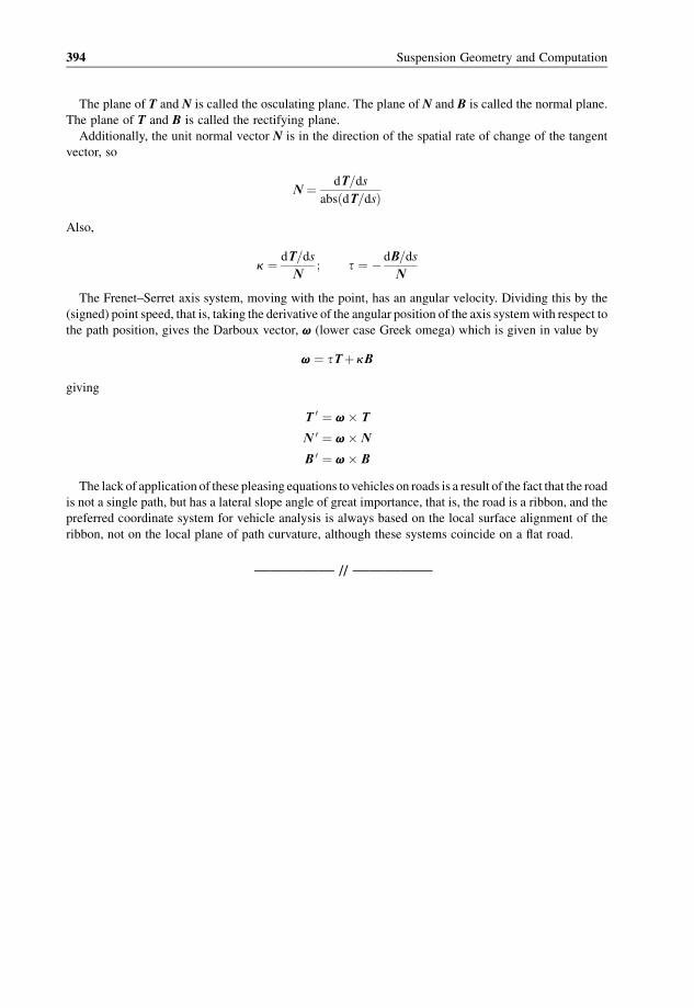
The plane of T and N is called the osculating plane. The plane of N and B is called the normal plane.

The plane of T and B is called the rectifying plane.

Additionally, the unit normal vector N is in the direction of the spatial rate of change of the tangent

vector, so

N ¼ dT=ds

absðdT=dsÞ

Also,

k ¼ dT=ds

N; t ¼ � dB=ds

N

The Frenet–Serret axis system, moving with the point, has an angular velocity. Dividing this by the

(signed) point speed, that is, taking the derivative of the angular position of the axis systemwith respect to

the path position, gives the Darboux vector, v (lower case Greek omega) which is given in value by

v ¼ tTþ kB

giving

T 0 ¼ v � T

N 0 ¼ v �N

B 0 ¼ v � B

The lack of application of these pleasing equations to vehicles on roads is a result of the fact that the road

is not a single path, but has a lateral slope angle of great importance, that is, the road is a ribbon, and the

preferred coordinate system for vehicle analysis is always based on the local surface alignment of the

ribbon, not on the local plane of path curvature, although these systems coincide on a flat road.

————— // —————


Appendix F

The Fourier Transform

F.1 Introduction

The Fourier transform is a representation of a periodic waveform by harmonic components, the method

having been invented by the French engineer andmathematician, J.P. Fourier (1768–1830), for analysis of

heat flux and temperature distributions. The method has subsequently found wide application throughout

the sciences (Newland, 1984; IEEE, 1967).

There are various types of transform, varying in the exact job and the method. The main acronyms to

know are:

DFT discrete Fourier transform

EFT engineering Fourier transform

FFT fast Fourier transform

FT Fourier transform

IDFT inverse discrete Fourier transform

IFT inverse Fourier transform

MFT mathematical Fourier transform

SFT slow Fourier transform

The discrete Fourier transform is the discrete transform of a discrete data set sampled from a continuous

periodic wave. Naturally, this lends itself to digital computation.

The fast Fourier transform is an efficient method of calculation of a discrete Fourier transform. It is

clearly defined mathematically, and would appear to be simple to use. In practice there are some

difficulties, not least because there are several extant programs that give differing results. This needs to be

explained. The first FFT algorithm was by C.F. Gauss in 1805 (published posthumously in 1866).

Theoretical analysis followed by Runge and Koenig in 1924, and a good algorithm by Danielson and

Lanczos in 1942.

In practical application, Fourier analysis is the representation of a cyclic (periodic) waveform by a

series of sine and cosine terms of various frequencies which sum to the original wave. For a continuous

original wave, the number of transformed frequencies is infinite. For a discrete (sampled) original data set,

as normally used nowadays, the discrete Fourier transform gives a number of frequencies basically equal

to half the number of points, that is,N data points (whereN is even) giveN/2 frequencies. Each of these has

a sine and cosine component, the amplitudes of which are calculated by the transform. Actually N points

give a top frequency N/2. The first frequency is actually zero, so the number of frequencies is a total of

N/2þ 1. This is two too many coefficients to determine from the N points. Two of the coefficients are


always zero. For the first and last frequencies (0 and N/2) the coefficients of the sine terms are

indeterminate, and therefore considered to be zero, having no significance. The zero cosine term

corresponds to the mean value. Because the frequencies begin at zero, it is convenient to number the

frequency array from zero. In practical computation of the DFT, it is efficient to use a data length N equal

to 2 raised to an integer power, N¼ 2M. Then a data array (1 :N) has N/2 frequencies numbered 0 to N/2.

For any one frequency, these two amplitudes can be combined into a total amplitude and a phase angle.

These amplitudes represent the spectral density. The wavelengths of the transform are given by the

original total wavelength of the data divided by successive integers. The frequencies are therefore in linear

progression.

The equations arewell conditioned, although subtractive cancellation is a possible problem. Numerical

accuracy is generally good. To perform a Fourier transform is to solve the N simulataneous equations for

the coefficents. The advantage of the Fourier transform is that the waves are orthogonal, so the results can

be obtained much more efficiently than for normal simultaneous equations. The fast Fourier transform is

normally used, but if only a few frequencies are required then a slow transform is acceptable, and is also

useful for checking purposes. The transform can be inverted to recover the data from the spectral

distribution.

This sounds straightforward, but in practice there are complications. There are various programs

available from several books, giving different results, which can bevery confusing.Also themethod of use

varies.

F.2 Types of Fourier Transform

There are several variations on the basic FT theme, and these need to be understood for correct use of a

DFT. The various programs can be classified in the following ways:

(1) Mathematical transform or engineering transform. The mathematical transform is the underlying

process. The engineering transform does a little morework, and actually produces the sine and cosine

coefficients, including the zero frequency terms (including themean)which are handled differently, or

starts with the sine and cosine coefficients and produces a data array.

(2) Dividing by N. If the bare mathematical process is applied, and then reapplied for an inverted

transform, the original data set is not recovered; instead the result is the original data set multiplied by

N. There is a variety of opinion onwhat to do about this. Some programs do nothing, some divide byN

at the forward transform stage, some divide by N at the inverse transform stage, and some make the

transform as symmetrical as possible by dividing byHN at both stages. To obtain agreement between

various published programs for themathematical transform it is therefore often necessary to adjust the

output up or down byN orHN. In the engineering transform, the divisionmust definitely be performed

exclusively in the forward direction to give the correct coefficients.

(3) Type of transform. There are two methods of transform, called Cooley–Tukey and Sande–Tukey, In

the FFT, there are two phases of operation. One is a bit rearrangement involving a two-deep loop. The

other is the basic transform itself involving a three-deep loop. In the Cooley–Tukey transform the bit

shifting is done first. In the Sande–Tukey transformation, the bit shifting is done last. Otherwise, they

seem to be considered equivalent, simply alternative methods that should produce the same results.

(4) Various published programs seem to give different numerical results when applied to a complex input.

If applied to a purely real input then they agree on the complexoutput. If applied to an imaginary input,

they have opposite signs for the complex output, which agrees in magnitude. If applied to a complex

input, they combine the complex parts to give not just sign disagreement but numerical value

disagreement. In some cases, it seems that the order of the coefficients is reversed. There is a unique

correct solution to the DFTof a given input data set, so there seems to be something amiss with some

published programs.

(5) Argument passing. In practical computation, the arguments are passed to subroutines in various

configurations. Programs for themathematical transform usually take a complex argument, that is, an


array of complex numbers (available as an intrinsic data type in Fortran). In languages without the

intrinsic complex data type, two real arrays may be passed, one with the real parts, one with the

imaginary parts, or a single pseudo-complex real array of alternating real and imaginary parts.

(6) Type of result. A basic engineering transform will typically accept a single real array argument and

return two arrays, the sine and cosine coefficients (or possibly the complete amplitude and phase

values). The MFT returns a complex array result.

(7) Number of input data sets. A goodmultiple EFTwill transform simultaneously two valid independent

real inputs (which correspond to the real and imaginary parts of a complex input in an MFT), so a

suitable engineering transform can accept two independent real arrays and simultaneously produce

the two real transforms (two independent sets of sine and cosine coefficients) in an efficient manner.

(8) In place or not. The transformationmaybe ‘in place’ or not, that is, the returned resultsmay replace the

incoming argument array or be returned as separate output arrays. It is usual for an MFT to take a

complex argument and to transform it in place, whereas an EFTwill usually take a data set and return

the transform in separate arrays without altering the data. The ‘in-place’methodwas once a necessary

memory saver, less necessary nowadays unless the arrays are very large, and not really good practice.

(9) There is more than one type of FFT, and the speeds vary considerably. One claimed FFTwas found by

the author to be a factor of 10 slower than the best program tried, although still faster than a slow

transform. Also, the SFT may be speeded up by various means, so there are SFT, fast SFT, slow FFT,

several varieties of FFT, and even very fast VFFT.

Considering the above alternative methods, configurations, argument passing conventions and per-

formances, the alternative Cooley–Tukey and Sande–Tukey transforms, and division by N orHN, or not,

the potential for confusion is apparent.

F.3 Engineering Fourier Transform

The EFT is firmly grounded in reality. The transform is between the data points in terms of definite

displacements from zero (e.g. the height of points along the road), and the amplitudes of the sine and

cosinewaves that correspond to, and can recreate, the positions. There is no room for discussion about the

signs, or about whether or not to divide byN orHN at various stages. The forward transform produces the

circular function (sine and cosine) amplitudes from the displacements, and the reverse transform produces

the displacements from the amplitudes. There is no ambiguity. To an engineer, the forward transform is

going from the data to the harmonic analysis (sine and cosine coefficients), and an inverse transform is

going from the frequency spectrum coefficients to a displacement data set. Therefore, as may be required

in practice, when starting with a frequency spectrum and producing a displacement array, the first thing

that an engineer may do is an inverse transform.

F.4 Mathematical Fourier Transform

In contrast, the MFT is less clearly defined, particularly in terms of when to do any divisions by the data

length. Here there seems to be a conceptual problem. The MFT is not grounded in reality as is an EFT, so

the MFT is whatever it is defined to be, and there seems to be no obvious way to check it against reality

without further processing, that is, to change it into an EFT. This leaves room for varying definitions, and

introduces the possibility of confusion. The mathematical definition typically given is

Hn �XN�1

k¼0

hk exp Sði2pkn=NÞ

where S is a signvalue, þ1 or�1. Changing the sign of S changes the direction of the transform.A process

with one sign followed by a process with the opposite sign is said to recover the data, but this is not entirely

The Fourier Transform 397

true. An increase by a factor of N occurs, requiring a compensating division by N at some stage, but it is

difficult to say exactly where this happens and at what point the correction should be introduced.

Mathematicians simply call it a Fourier transform whichever way it is used first, and then an inverse

transform is going back the other way. This contrasts sharply with the engineer’s idea of forward and

inverse transforms, in which the data in the two forms have different physical meanings – for example, in

one case a series of point heights along a road, in the other a series of amplitudes of sines and cosinewaves.

F.5 Mathematical Definitions

Press et al. (1992) give the forward transform definition as

Hn �XN�1

k¼0

hk exp ði2pkn=NÞ

where the data set is h(0 :N�1), with n, the index of the various frequencies, running from 0 to N/2. The

inverse transform is given as

hk � 1

N

XN�1

n¼0

Hn exp ð�i2pkn=NÞ

with a division by N clearly stated to be in the inverse transform only. The forward transform has no

negative sign in the exponent, which appears in the inverse transform only.

In contrast, Newland (1984) gives the formal definition of the ‘forward’ transform as

Xk ¼ 1

N

XN�1

r¼0

xr exp ð�i2pkr=NÞ; k ¼ 0; 1; 2; . . . ;N�1

and the ‘reverse’ transform as

xr ¼XN�1

k¼0

Xk exp ði2pkr=NÞ; r ¼ 0; 1; 2; . . . ;N�1

exhibiting not only a difference inwhen to divide byN, which nowappears in the ‘forward’ transformonly,

but also changing of the signs in the exponents, with the negative exponential sign now occurring in the

forward transform. In effect, then, the definitions of forward and reverse transforms have been

interchanged.

In Harris and Stocker (1998) the forward transform is expressed (with slightly changed notation) as

fr ¼ 1

N

XN�1

k¼0

ck expði2pkr=NÞ

agreeing with Press et al. There is no explicit statement of any reverse transform.

F.6 Equations

The data set is Y(J) with J¼ 1 :N. The numberN is preferably, for convenience and efficiency in an FFT, a

whole power of 2. In any case, the equations vary slightly for an odd number of points, so an even number

is assumed, even for the SFT. The independent variable X is equally spaced at DX. The first wavelength isl¼NDX. The notional point number Nþ 1 is the first point of the next wave, and has the same Y value as


the first point of the data set, Y(Nþ 1)¼ Y(1). This can be used as a check in the regeneration of the

data. The independent variable for point J is X(J)¼ (J�1)�DX with the first point at X(1)¼ 0. The last

point is at X(N)¼ (N� 1)�DX. The first point of the next wave is at X(N)¼N�DX.The lowest frequency is zero. The top frequency is M¼N/2. The total number of frequencies is

Mþ 1¼N/2þ1. The data set (points J¼ 1, . . . , N) is produced from the trigonometric function

coefficients by the slow inverse-transform equation

YðJÞ ¼ 1

2C0 þ

XM�1

K¼1

CK cos2p JK

N

� �þ SK sin

2p JK

N

� �� þ 1

2CM cosðpJÞ

Here it is apparent that the first and last frequencies (K¼ 0 and K¼M¼N/2) have no sine term (no SKcoefficient).

To obtain the trigonometric coefficients from the data, the slow forward-transform equations are

CK ¼ 2

N

XNJ¼1

YðJÞ cos�2p JK

N

�; K ¼ 0; 1; . . . ;N=2

SK ¼ 2

N

XNJ¼1

YðJÞ sin�2p JK

N

�; K ¼ 1; 2; . . . ;N=2� 1

where J is the data index and K is the frequency index. For the sine coefficients, it is apparent here that

for K¼ 0 the sine argument would be zero, so the value of S0 is zero. For K¼N/2, the sine argument is

a multiple of p and would give SN¼ 0.

Considering the complex coefficient

ZK ¼ CK þ iSK

then the transform into trigonometric coefficients may be expressed as

ZK ¼ 2

N

XNJ¼1

YðJÞ�cos

�2p JK

N

�þ i sin

�2p JK

N

��

¼ 2

N

XNJ¼1

YðJÞ exp�i2p JK

N

�; K ¼ 0; 1; . . . ;N=2

The fact that the product JK occurs with integer values ranging from 1 to N and from 0 to N/2

respectively gives an integer product range from 0 to N2/2. This makes possible a more efficient

calculation of the slow transform, by precalculating the necessary sine and cosine values – an FSFT.

Also, the slow transform may often be applied for a limited frequency range, or for a limited number of

frequencies that are of interest. The FFTof necessity does all frequencies, many of which may not be of

much engineering interest. The practical speed gain of the FFT, whilst very valuable, is therefore a little

exaggerated.

Comparing the equations here, for the SFT,with the earlier definitions for theMFT, it is apparent that the

SFT has an additional factor 2, and divides by N in the forward direction.

F.7 Published Programs

The FORK program is an MFT by V. Herbert (1962) (pre-dating Cooley and Tukey (1965), who were,

however, the first to publish in recent times), modified by Brenner, and further modified and published by


Claerbout (1975). It works correctly in all respects. It divides by HN in both directions, so it is

symmetrical, and it has a direction switch argument to provide forward and reverse transforms. It has

bit reversal first (Cooley–Tukey).

The MFT program Four1 in Press et al. (1992) is stated to based on ‘a program by Brenner’. It does not

do a division in either direction. It produces the correct signs. There is a direction switch. Bit reversal is

first (Cooley–Tukey). With adjustment for the division, it is in good agreement with FORK.

The MFT program in Newland (1984) has no switch, being intended for forward transforms only.

It includes division by N. An appendix explains how to reverse it, including, inter alia, removal of the

division. Bit reversal is first. The signs for the imaginary part of the argument appear to be wrong, so it

works for the real part only. Newland has a usefully different way of handling some of the details.

TheMFT program in Harris and Stocker (1998) is in pseudo code. It is easily expressed in Fortran. It is

stated to be Sande–Tukey, and does indeed have the bit reversals last. It accepts two real argument arrays,

but apparently produces thewrong signs for the second one, so the output appears correct only for a single

real array. It is intended for forward transforms only, and there is no explanation about how to reverse it.

Barrett andMackay (1987) provide a program in Basic which they describe as based on the ‘successive

doubling’ method. This converts readily to Fortran, but seems relatively slow (by FFT standards) and

works for a single real array only, giving incorrect signs for the second input array.

Various other published programs have been investigated with a view to use, but have generally been

found wanting in one way or another. Typically they are either incorrect or very slow by good FFT

standards.

F.8 Dividing by N

For the MFT, it is desirable for successive forward and reverse transforms (or vice versa) to recover the

original data, which end up multiplied by N in the bare process, so a compensating division by N should

occur somewhere around the two-way cycle. For symmetry, this can be a division byHN in each process.

However, it is more efficient to do a single division at one stage.

For the EFT, the forward transform requires a division byN to obtain the correct coefficients. If theMFT

in use does a division byHN then the EFT must do a further division, which is not ideal. For the reverse

transform, no overall division is needed, so if the MFT does a division then the EFTwrapper must do a

compensating multiplication.

Therefore, for efficient operation of theEFT, it is better if theMFTin use does noN orHN division at all,

or does the division by N in the forward transform only. Because the EFT has an additional factor of 2 to

deal with anyway, the most efficient computation is achieved if the factoring is left entirely to the EFT

stage, with no divisions in the basic MFT.

The best solution, then, is probably to have an underlying service routine that does no divisions. The

MFT will use this and add its own divisions by HN in both directions, keeping it symmetrical and

providing reversibility. The EFT will also use the underlying routine, and can do so in its own way

efficiently.

F.9 Sign Discrepancies

When the data are placed in the imaginary part of the complex argument of anMFT, or if two data sets are

processed simultaneously, or if the transformof a complexdata set is required, there is disagreement on the

results from the various published programs (not just those listed above). If only one real data set is used,

placed in the real part of the complex argument of the MFT, there is agreement on the result. The fact that

the programs agree in this simple case has increased the confusion.When theMFT is used in the service of

an EFT, as it generally is for practical applications, the sine and cosine amplitudes are deduced from the

complex coefficients found by the MFT. This process involves taking the symmetric and antisymmetric

aspects of the output, adding and subtracting corresponding terms invariousways.With the output froman


MFT that has faulty signs, the error can be corrected by changing (fiddling) the signs used in the additional

EFT processing. Therefore the final result of the EFTmay still be correct, because of compensating errors.

This seems to have disguised the fact that there is inconsistency in the output of publishedMFT programs.

However, twowrongs do not make a right, and it seems that some of the publishedMFT programsmust be

incorrect in their signs. If two programs differ in themagnitude or sign of their output, one of themmust be

wrong, unless there is ambiguity in the definition of the FT.

F.10 Speed

There are significant differences in the speed of various FFTs. There are some slow ones around that are a

factor of 10 worse (successive doubling method) than a good standard one. There are various ways to

improve the performance of even a good one, for example by using a base-4 transform, which can be 20%

faster than a conventional FFT, promotion of unnecessary calculations out of inner loops, careful

organisation of exit conditions or use of determinate loops. When only one real array is to be processed,

it may be expected that it would run faster than a double array (or complex array) because the zero

imaginary parts will process more rapidly, but this seems to be a small effect in practice. A further

improvement may still be possible by using a folded single array in a complex half-length array; see the

Press et al routine ‘realft’.

F.11 Equation Check Program

The following program is purely for checking the FT equations for consistency.

!

!

! TEST DFT EQUATIONS

!

!

Program Test_FT_Eqns

Implicit none

Integer J,K,KD,KF,N,ND,NF,M,IT

Real*8 d(1024),dr(1024),de(1024),a(0:512),b(0:512),RandH

Real*8 pi,s,sa,sb,t,er

IT=0

Print*

Print*,’Numerical check of DFT equations by slow FT:’

Print*

pi=acos(-1d0)

ND=1024

Print ’(A,I0)’,’ ND = ’,ND

Do KD=1,ND

d(KD)=RandH()

enddo

If(IT>0)Print*,’Start analysis:’

NF=ND/2

Do KF=1,NF-1

sa=0

sb=0


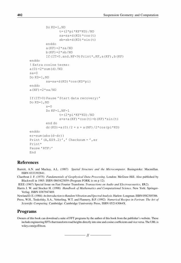
Do KD=1,ND

t=(2*pi*KF*KD)/ND

sa=sa+d(KD)*cos(t)

sb=sb+d(KD)*sin(t)

enddo

a(KF)=2*sa/ND

b(KF)=2*sb/ND

If(IT>0.and.NF<9)Print*,KF,a(KF),b(KF)

enddo

! Extra cosine terms:

a(0)=2*sum(d)/ND

sa=0

Do KD=1,ND

sa=sa+d(KD)*cos(KD*pi)

enddo

a(NF)=2*sa/ND

If(IT>0)Pause ’Start data recovery:’

Do KD=1,ND

s=0

Do KF=1,NF-1

t=(2*pi*KF*KD)/ND

s=s+a(KF)*cos(t)+b(KF)*sin(t)

end do

dr(KD)=a(0)/2 + s + a(NF)/2*cos(pi*KD)

enddo

er=sum(abs(d-dr))

Print ’(A,ES9.2)’,’ Checksum = ’,er

Print*

Pause ’RTF:’

End

References

Barrett, A.N. and Mackay, A.L. (1987) Spatial Structure and the Microcomputer. Basingstoke: Macmillan.

ISBN 0333392841.

Claerbout J. F. (1975) Fundamentals of Geophysical Data Processing. London: McGraw-Hill. Also published by

Blackwell in 1985: ISBN 0865423059 (Program FORK is on p 12).

IEEE (1967) Special Issue on Fast Fourier Transform. Transactions on Audio and Electroacoustics, 15(2).

Harris J. W. and Stocker H. (1998) Handbook of Mathematics and Computational Science. New York: Springer-

Verlag. ISBN 0387947469.

NewlandD.E. (1984) An Introduction toRandomVibration andSpectral Analysis.Harlow:Longman. ISBN0582305306.


Scientific Computing. Cambridge: Cambridge Uuniversity Press, ISBN 052143064X.

Programs

Owners of this book can download a suite of FFT programs by the author of this book from the publisher’s website. These

includeengineeringEFTs that transformroadheights directly into sineandcosinecoefficients andviceversa.TheURLis

wiley.com/go/Dixon.

————— // —————


References and Bibliography

References

Adams, D.A. (1967) A stopping criterion for polynomial root finding. Communications of the ACM, 10(10), 655–658.

Bolaski M. P. (1967) Front Vehicle Suspension with Automatic Camber Adjustment, US Patent 3,497,233, filed 3 Nov

1967, patented 24 Feb 1970.

Cebon D. and Newland D. E. (1984) The Artificial Generation of Road Surface Topography by the Inverse FFT

Method, in 8th IAVSD Conference on Dynamics of Vehicles on Roads and Tracks, pp 29–42. Lisse: Swets and

Zeitlinger.

Conte S. D. and De Boor C. (1972) Elementary Numerical Analysis: An Algorithmic Approach, 2nd edn. New York:

McGraw-Hill. (A classic, well worth seeking out second hand.)

Dixon J. C. (1991) Tyres, Suspension & Handling, 1st edition, Cambridge University Press.

Dixon J. C. (1996) Tires, Suspension and Handling, 2nd edition, London: Edward Arnold, ISBN 0340677961 (In US

SAE, ISBN 1560918314).

Dixon J. C. (2007) The Shock Absorber Handbook, Chichester: J. Wiley & Sons Ltd, ISBN 9780470510209.

Drechsel A. (1956) Radf€uhrungsanordnung f€ur Fahrzeuge, German Patent 12-14-100, filed 18 Dec 1956, patented 10

Nov 1966.

Durstine, J. W. (1973) The Truck Steering System from Hand Wheel to Road Wheel, SAE 730039, The 19th Ray

Buckendale Lecture, January 1973, SAE SP-374, New York: Society of Automotive Engineers.

Ford H. (1937), Motor Vehicle, US Patent 2,214,456, filed 1 Nov 1937, patented 10 Sep 1940.

Hamy N. (1968) The Trebron DRC Racing Chassis, Motor, Dec. 21, 1968, pp. 20–24.

Heldt, P. M. (1948) The Automotive Chassis, 2nd edition, Published by P. M. Heldt, 600pp.

Hurley L. G. (1939) Automobile Chassis, US Patent 2,279,120, filed 5 Jun 1939, patented 7 April 1942.

Jeandupeux P. A. (1971) Suspension pour V�ehicules Automobiles, Swiss Patent 537818, filed 4May 1971, patented 31

July 1973.

Jenkins, M.A. (1975) Zeros of a real polynomial (Algorithm 493), ACM Transactions on Mathematical Software,

1(2), 178–189.

Jenkins, M.A. and Traub, J.F. (1972) Zeros of a complex polynomial, Communications of the ACM, 15(2), 97–99.

Katz A. (1997) Computational Rigid Vehicle Dynamics, Malabar, Florida: Krieger Publishing Company, Inc., ISBN

1575240165. (Discussion of calculation and use of quaternions.)

Lapidus L. (1962) Digital Computation for Chemical Engineers, New York: McGraw-Hill. (Hard to find. Good

explanations of general numerical methods. The chemical content is limited to the end-of-chapter examples.)

MacPherson E. S. (1949) Wheel Suspension System for Motor Vehicles, US Patent 2,660,449, filed 27 Jan 1949,

patented 24 Nov 1953.

Madsen, K. (1973) A root-finding algorithm based on Newton’s method. BIT, 13, 71–75. (Includes a program in

ALGOL.)

M.I.R.A. 1965/1 Definition of Handling Terms.

Morrison J. L.M. and Crossland B. (1970)An Introduction to theMechanics ofMachines, 2nd edn in SI units, London:

(Longman. ISBN 0582447291 and 0582447313. Contains material on velocity and acceleration diagrams.)


Muller, D.E. (1956) Amethod for solving algebraic equations using an automatic computer,Mathematical Tables and

Other Aids to Computation, 10, 208–215.

Nemeth J. (1989)Optimization on steeringmechanisms for high speed coaches, In Second International Conference on

New Developments in Powertrain and Chassis Engineering, pp 325–330, Bury St Edmunds, Mechanical Engineer-

ing Publications, ISBN: 0852986890.

OpenUniversity, Course T235EngineeringMechanics – Solids contains detailedmaterial on drawing velocity diagrams.

The entire course (on basicmechanical engineering) is available free at http://intranet.open.ac.uk/open-content/. Click on

�Visit the OpenLearn website�, enter �LabSpace�, click on topics �Technology�, go to page 3, scroll down to �EngineeringMechanics: Solids� and click on �Browse�. See Block 3 for velocity diagrams.

Ostrowski, A.M. (1973) Solution of Equations in Euclidean and Banach Space, New York: Academic Press.

Parsons C. F. D. (1969) Vehicle Wheel Suspension System, US Patent 3,598,385, filed 27 Mar 1969, patented 10 Aug

1971.

Pellerin L. (1997) Vehicle Suspension System, UK Patent GB2309206, priority date 19 Jan 1996, filed 17 Jan 1997,

patented 11 Mar 1998.

Phillippe M. P. (1975) Vehicle Suspension Systems, UK Patent 1526970, filed 30 Dec 1975, patented 4 Oct 1978.


Scientific Computing, Cambridge: Cambridge University Press, ISBN 052143064X. (Also available in C and Basic.

Well known reference, more-or-less essential, many programs, although no help on geometry.)

Rall, L.B. (1966) Convergence of the Newton process to multiple solutions. Numerische Mathematik, 9, 23–27.

Robson J. D. (1979) Road Surface Description and Vehicle Response, International Journal of Vehicle Design,

1(1), 25–35, Inderscience.

SAE (1976) Vehicle Dynamics Terminology, SAE J670e,Warrendale, PA: Society of Automotive Engineers (included

as an appendix in Dixon, 1996, above).

Schr€oder, E. (1870) Uber unendlich viele Algorithmen zur Aufl€osung der Gleichungen. Mathematische Annalen, 2,

317–365.

Shoup T. E. (1979) APractical Guide to ComputerMethods for Engineers, Englewood Cliffs, NJ: Prentice Hall, ISBN

0136906516. (Good explanations.)

Shoup, T.E. (1984) Applied Numerical Methods for the Microcomputer. Englewood Cliffs, NJ: Prentice Hall. ISBN

0130414182. (This is a development of Shoup, 1979.)

Sloan A. P. (1963) My Years with General Motors, Doubleday.

SpiegelM. R. (1968)Mathematical Handbook of Formulas and Tables, NewYork:McGraw-Hill, ISBN 0070382034.

Sternberg E. R. (1976) Heavy Duty Truck Suspensions, S.A.E. Paper 760369.

Verschoore R., Duquesme F. and Kermis L. (1996) Determination of the Vibration Comfort of Vehicles by Means of

Simulation and Measurement, European Journal of Mechanical Engineering, 41(3), 137–143.

Walker P. (2008) Camber Nectar, US patent 7407173, filed 29 May 2003, patented 5 Aug 2008.

Weiss W. (1997) Wheel Suspension with Automatic Camber Adjustment, US Patent 6267387, filed 12 Sep 1997,

patented 31 July 2001.

Bibliography

For a qualitative discussion of many example suspensions, see Norbye (1980). Amore quantitative analysis with many

practical examples is given in Campbell (1981) andBastow et al (2004). Formore examples specifically on front-wheel

drive see Norbye (1979). Sternberg (1976) above is a useful reference on the suspension of heavy commercial vehicles.

Many details of suspension design from old, previously unpublished, General Motors reports by Olley have been

gathered together with added explanation by Milliken and Milliken in Olley et al (2002), which also gives historical

insight. Matschinsky (2000) gives a useful analysis of suspensions in some depth. See also Dixon (1996) and (2007)

above.

Bastow D., Howard G. and Whitehead J. P. (2004) Car Suspension and Handling, 4th Edn, Professional Engineering

Publishing, ISBN 186058439X. (In US, SAE, ISBN 0768008727.)

Campbell D. (1981) Automobile Suspensions, Chapman and Hall Ltd, ISBN 0412164205. (A general introduction to

vehicle suspensions.)

MatschinskyW. (2000) Road Vehicle Suspensions, Bury St Edmunds: Professional Engineering Publishing Ltd, ISBN

1860582028.


Milliken W. F. and Milliken D.L. (1995) Race Car Vehicle Dynamics, New York: Society of Automotive Engineers,

ISBN 1560915269.

Norbye J. P. (1979) The Complete Handbook of Front Wheel Drive Cars, Tab Books, ISBN 0-8306-2052-4.

Norbye J. P. (1980) The Car and Its Wheels – A Guide to Modern Suspension Systems, Tab Books, ISBN 0-8306-

2058-3.

Olley M., Milliken W. F. and Milliken D. L. (2002) Chassis Design Principles and Analysis, New York: SAE, ISBN

186058389X.

————— // —————

References and Bibliography 405

Index

After the page number, a letter e means a significant equation, f means a figure, p means an example

program fragment or program output, and t means a table.

Acceleration, angular 58e

diagrams 297

diagrams, in 3D 350

iteration factor 344

normal 51e

Accelerometer, zero 63

Accuracy, lost 326

of program 330

Ackermann 2, 3, 13, 16, 112, 118, 244

angle 101f

factor 103, 104ef, 105f, 106e, 108e

steering arms 107ef

ACOS, bad argument 326

Adams 343, 357, 403

Aitken’s acceleration 345e

Alfa Romeo T-bar 21f

Aliasing 77

Angle, Basic function 70

bump camber 144e

bump caster 194e

camber 119e, 144ft

caster 118e, 193e, 199e

compliance 182f

inclination 118f, 144ft

path etc 57ef

phase 70f

pitch 190e

roll steer 134e

steer 127e

Anti-dive, etc 13, 190f, 191t

etc, design 193

Anti-roll, coefficient 164e

Antisymmetry 71

Arm, see also Single arm, Double arm

angled 230f

double see Double arm

length, and angles 229f

length, difference 232f, 233e

length, equal 230ft

semi-trailing 207f

semi-trailing, low pivot 209

semi-transverse, 215f, 216t

semi-transverse, low pivot 216

single see Single arm

transverse 210–212ft

transverse, sloped axis 212f, 213t

transverse, sloped axis,

elimination of bump force 213e,

214f

Arms, converging 231ef

double, see Double arm

parallel trailing 14f

ASIN, bad argument 326

Assembly problem 332–334fp

Aston Martin 14f

Atan2, Fortran function 70

Attitude angle, kinematic 102ef

Audi, undriven rear axle 25f


Axle, see also Rigid axle

bending 1

camber 150e

four-link 21f

inclination and camber 145

roll 92f

roll inclination angle 147e, 148e

steer 132

steer, angles 131, 132e

tramp 20

tweaking 156

Bairstow 352, 353e

Banking 51f, 71, 72

Barrett 402

Bastow 10, 404

Belgian pav�e 44

Bennett, suspension 37f

Benz 3, 5, 99, 107, 108f

Bibliography 404

Bicycle, model 100

Binary search 338

Binormal 393

Block (sliding) axle location 160f

Blunder 330

BMW 9f, 29f

Bolaski 39f, 403

Bolle�e 2, 3

Bounce 88

Broulhiet 13

sliding pillar 12f

Buick 11

Bump, 88

and roll, non-linear 149

camber 145ef

camber angle 144e

double 88

double, symmetrical on GRC 165, 166ef

from roll 147ef

isolated 67t

rectangular 74

scrub 153

scrub rate 153

scrub, single arm 224f, 225ef

shape 67t, 68f

single, symmetrical on GRC 167ef

steer, see also coefficient

steer 7, 10

steer, axle linear 134

steer, dimensions 129t

steer, graph 131f

steer, models 196

steer, non-linear 134e

suspension 83

Cadillac, independent front (1934) 11f

Camber, see also Axle, Inclination, Wheel

angle 119e, 144ft

bump 145ef

static 147e

wheel 143

wheel and road 146f

Camber Nectar 42f

Campbell 404

Car turn-in 59e

Cart steering 2f

Caster, angle 118ef, 193e, 199e

centrifugal 119

Cauchy 350, 352

Cebon 44, 63, 403

Chapman strut 29f, 30f

Checksum 334p

Chevrolet 11

Circle, in 3D 308e

Circular motion 56e

Citro€en, undriven rear axle 26f

Claerbout 400, 402

Coefficient, aligning moment compliance

steer 185

anti-dive, etc 191t, 192t

anti-lift 191t, 192e

anti-rise 191t, 192e

anti-roll 164e

anti-squat 191t, 193e

axle roll, camber 144t

axle roll, from bump 148e

axle roll, inclination 153e

axle roll, steer 132e, 133e

bump camber 144t, 152e, 195

bump camber, converging arms 232e

bump caster 118, 194e

bump kingpin caster 195

bump kingpin inclination 196

bump scrub 153

bump scrub rate 153, 195

bump scrub rate variation 154ef, 195

bump steer 128e, 130e, 195

bump to/from roll/toe 135e

double arm, bump camber 285e, 286e

double bump steer 136e

408 Index

kingpin caster 222e

kingpin inclination 222e

lateral force compliance camber 185

lateral force compliance steer 185

overturning moment compliance camber 185

rigid axle, heave pitch 260e

rigid axle, understeer 259ef

roll camber 152

roll inclination 144t

roll scrub 156e

roll steer 134e, 135e

roll toe 135e

scrub rate, lateral, longitudinal, 223e

scrub rate, locked wheel 223e

steer camber 119e

steer caster 124e

steer inclination 124e

steer jacking 125e

strut, bump camber 246et, 249, 288e

strut, bump caster 246et

strut, bump scrub 246et

Coefficients, different arm lengths 233e

double arm lateral 227

double arm longitudinal 227

double arm, bump camber 236et

double arm, bump caster 241et

double arm, bump scrub X 241et

double arm, bump scrub Y 236et

double arm, lateral 236et

parallel level arms 230t

rigid axle, 256t

semi-trailing arm 208e, 209t

trailing arm 201t, 202e, 203et, 205t

trailing arm, sloped axis 206t

transverse arm 212t, 213t, 216t

Coherence, track 80, 81f

Compliance, see also Steering 88

angles 182f

experimental 188

hub centre forces 186

inclination angle 185e

matrix 183e, 184

ride 184e

rigid axle steer 187

steer angle 186e, 187

steer coefficient 186e

steer gradient 185, 186e

steer, control of 179

steering 187

Compound crank axle, see Trailing twist axle

Conditioning, bad 328e

Contact patch, angle subtended 85e

area 83

length 70, 85e

Conte 347, 357, 403

Convergence, accelerated 344–346e

cubic 338

failure 326

linear 337e

of iteration 337

per evaluation 338

quadratic 338

Conversion factors 378t

Cooley 399, 400

Coordinate system, wheel, ISO 180f

wheel, SAE 180f

Coordinates, cylindrical 299

non-rectangular 299

transformation 300e

Cornering, force, zero banking 52e

test, rough 74

Cosine rule 304ef

Cosines, direction 300e

Cottin-Desgouttes 10f, 26

Crossland 298, 403

Curvature angle, wheelbase 51e

normal 50e

path 48t, 49f

Danielson 395

Darboux 393

Darwin 3

Data out of range 326

Data sensitivity problem 329e, 330ep

Data trend, effect 75, 76f

removal 76

De Boor 347, 357, 403

De Dion 23f, 24f, 133, 156

Decimetre 377

Delta-squared process 346e

Derivative of a quotient 168

Design process, double arm 236

DFT 75, 395

Direction cosines 300e

pivot axis, 198f, 199e, 199t

wheel axis 116et

Direction numbers 300e

Discomfort, passenger 96e

tyre 96e

Displacement v. length 300

Index 409

Divergence, of iteration 339

Division by zero 326

Dixon 138, 141, 159, 178, 188, 403

dm 377

Double A-arm, see Double arm

Double arm, angle relationships 235et

configurations 228f

design process 236

examples 16–18

Ford 29f

general solution 233, 234eft

lateral coefficients 236et

longitudinal 240ef, 241et

numerical 2D solution 237, 238ft, 239t

numerical 3D solution 242t

suspension 227

Double lateral arm, see Double arm

Double trailing arms 250, 251 etf

Double transverse arm, see Double arm

Double wishbone, see Double arm

Double-bump steer 136e

Drechsel 37f, 403

Driveshaft, plunge 10f

Droop 83

strap 21f

Dubonnet 10, 12f, 13, 227

Duquesne 81, 82, 404

Durstine 100, 125, 403

Dynamic index 133

Ease of use 332

Edgeworth 3

EFT 395

Electrostatic analogy 352

Elliptics 3

Equivalent link, accuracy 260

leaf spring 140

Error block 327p

ratio, iteration 339

relative 337

Exit, iterative 340

Failed to converge 326

Failure Modes Analysis 326

Fairthorpe TX-1 37f

FFT 75, 395

Fiat 9f

leaf spring 20f

leaf spring with coils 21f

traction bar 20f

Five-link axle 31f, 251

Flannery 357, 402, 404

Foot, see perpendicular

Force, hub centre 186

see also Wrench

tractive, equivalent system 186e

Ford 29f, 226, 403

Capri 7

four-link 21f

strut rear 33f

FORK program 399, 400

Fourier 395

analysis 75e

build-up 76f

transform 395–402e

transform, download URL 402

FRC 162–164

Frenet 393

Frequencies, successive 76f

Frequency 69e

dividing 46

spatial 69e

FT 395

Galileo 381

Garwick’s device 343

Gauss 395

Gaussian rms 96

Glas Isar 15f

Gordon-Armstrong 14f

GRC 164–165

Gyro precession 7

Gyros 63

Halley’s iteration 349e

Hamilton 381

Hamy 37f, 403

Harris 398, 400, 402

Haversine curve 67fe

Heading angle 57ef

Heave 83, 88, 89f

steer, vehicle 137e

Heldt 125, 403

Herbert 399

Hillman, swing arm 15f

Hotchkiss 140

axle 20

Howard 404

Hub centre forces 186

Hurley 36f, 403

410 Index

Ideal rack position 244

IDFT 395

IE (IERR) values 326

IEEE, real number 331

IFT 395

Inclination, see also Camber

angle 118f, 144ft

axle roll 149e

roll, from bump camber 148e

wheel 143

Inclinometer 63

Installation ratio, see Motion ratio 271

Intersection, 2 spheres and horizontal plane 319e

3 planes 319–320e

3 spheres 316–318e

line and plane 320e

Iteration 335

see also Convergence

accelerated 344–346e

accelerated fixed-point 356t

adaptive speed factor 344e

Aitken 345e

Bairstow 353e

bracketing 341

Cauchy 350e

comparison of methods 355–356t

convergence 337

correction factor C 350e

delta-squared process 346e

endogenous 343

exit 340–341p

exit condition 342

exogenous 343

factor 339, 344

fixed-point 343, 356t

group g 350

Halley 349e

high order 351 et

high order, no derivatives 346

Laguerre 252e, 351

Lin 353e

linear 340et

linear, problems 339

Madsen 352

Muller 347–348e

multiple root 349e, 352

Newton 348e

Newton with 3D-VD 356t

Newton’s second 349e

Newton-Raphson 348e

Olver 2350e

Parlett’s criterion 352

phase detection 342, 343

regula falsi 347

relaxation factor 344

Schr€oder 349

secant 346f, 347e, 356t

see also convergence

solution of axle 261

speed factor 344

staircase 342f

Steffensen 345e

three phases 336 ef

Jacking, link 162e

spring 91

steer 124

Jaguar 16f

Jeandupeux 40f, 403

Jeantaud diagram 106

Jenkins 343, 352, 357, 403

Jerk 56e

Katz 392, 403

Kermis 81, 82, 404

Kilopond 377

Kingpin axis, see Steer Axis

Koenig 395

KRC 160–162

K-squared rig 10

L’Obeissante 2f

La Mancelle 3f, 107, 108f

Laguerre 338, 351, 352

Lancia, Lambda 13

semi-trailing arm 28f

sliding pillar 13

strut rear 33f

transaxle 28f

undriven rear axle 26f

Lanczos 395

Langensperger 2f, 3

angle 103e, 104, 105f

Lapidus 357, 403

Leaf springs, equivalent link 140

Leap, away from root 339

Length v. displacement 300

Lift bar 133

Lin 352, 353e

Line 305

Index 411

Line, parametric form 305e, 306e

rotation about a second line, 217

see also Intersection

standard form 305e

Link jacking force 162e

Load transfer, factor 164e

longitudinal, 189e

LOG, bad argument 326

Logger analysis 61–63

London taxi 104

Lunar Rover 104

Mackay 402

MacPherson 403

strut 18f

Macrostructure, road 77f

Madsen 352, 357, 403

Maserati, leaf spring 6

Matra Simca, trailing arms 28f

Matrix, steering compliance 183e, 184

Matschinsky 404

Mercedes Benz 5f, 9f, 16f, 17f, 27f, 31f

GP 1908, 5f

low pivot swing axle 27f

multilink 31f

MFT 395

Microstructure, road 77f

Milliken 405

MIRA 44, 403

Morrison 298, 403

Motion ratio 271, 272 et, 273e

displacement method 274

displacement test 275

effect on damping 293, 294e

effect on inertia 290, 291e

effect on stiffness 292e, 293et

pushrod, pullrod 288

rocker 276

spring 284e

velocity diagram method

Muller 347, 348, 357, 404

Muller’s method 347–348e

Multilink axle, 31f, 251

Multiplier, ideal iteration 339

Nemeth 109, 125, 404

Newland 44, 63, 395, 398, 400, 402

Newton 343, 348, 352

Newton-Raphson iteration 348e

Noise, white, pink 80

Norbye 405

Number, real, representation 330

Offtracking 101e

zero 103

Oldsmobile 11

Olley 10, 405

Olver 350

Opel, de Dion axle 23f

independent 12f

rear axle 22f

strut 19f

trailing twist 34f, 35f

Open University Course T235 298,

404

Optimisation, program speed 331

Orthogonal vector 218

Oscillation, of iteration 339

Ostrowski 349e, 357, 404

Oversteer, side force 26

Panhard rod 22f, 25f, 139

Panhard-Levassor 100

Parallelogram linkage 113f

Parametric representation 45

Parlett’s criterion 352–353

Parsons 39f, 404

Passenger, on seat 88, 89f

Path, see also Road, Track

analysis 53–55

angle 48t, 54ef, 57ef

antisymmetrical 71e

curvature 48t, 49f, 54e, 393

length 45

profile, building 80

radius change 58e

turn-in 54e, 59e

two-track, phase angle 72f

Pellerin 41f, 404

Perch (point above triangle) 315

Period, of oscillation 69e

Perpendicular, onto 3-point plane

315e

onto a line 309e, 310e

onto a triangle 313e

onto normal-form plane 314e

Phase angle 70f

two-track 72f

Phillippe 40f, 404

Pink noise 80

412 Index

Pitch 83, 90

geometry 189

steer, vehicle 137e

Pitman arm 11f, 112

Pivot axis, direction cosines 198f, 199e, 199t

single-arm suspension 196, 197f

Plane, general form 306e

intercept form 306e

normal (N&B) 394

normal form 306e

normal form, from 3 points 313e

osculating 394

radical 308e

rectifying 394

through 3 points 306e

Plunge, driveshaft 10f

Point, see also Intersection, Velocity

above a triangle 315, 316ef

in 3 planes 319–320e

in a triangle 310e, 311ef, 312e

intersection of 3 spheres 316–318e

of line and plane 320e

specification 305

Polynomial, roots 351–356etp

Pontiac 11

Porsche, �917’ suspension 86

Weissach axle 30f

Position v. length 300

Pound, mass as kg 377

PRCC, suspension 41f

Precision, 8-byte number 337

quad 331

Press 352, 357, 398, 402, 404

Pro-dive 13

PSD 78

Pseudo-force, normal 51e

Pullrod, motion ratio 288

Pushrod, motion ratio 288

Pythagoras, in 3D 299

Quadratic, solution 348

Quarter-car model 88

Quaternions 381–392

cf complex numbers 390

Rack, helix angle 113

Radian 377

Radical plane, of spheres 308e

Radius, see also tyre, wheel

cornering 100ef

loaded 84, 94e, 119

of curvature 48, 49f

rolling 119

rolling, effective 84

tyre 84

unloaded 84

Rall 349, 357, 404

Ramp, haversine 66f

isolated 65, 66tf

linear 66f

Raphson 348

RASER value 325

Real number, representation 331, 337, 338

References, collected 403

Reliability, of program 327p

Renault, offset torsion bar 32f

swing axle 27f

trailing arms 32f, 34f

undriven rear axle 24f

Ride analysis, frequency domain 96

time domain 95

Ride, height 92

meter (Olley) 10

position 88, 89ef

Rigid arm, velocity ratio 283e

Rigid axle 253, 254f

coefficients 256t

compliance 187

example results 264–270

examples 266f, 268f

leaf with steering 140, 141f

link analysis 258ef

location 138

numerical 3D solution 260

pivot point roll steer analysis 257e

points defined 260

roll centre 256e

roll, steer pitch angles 255ef

steered 7f

velocity diagram 289f, 290f

with leaf springs 140

Rigid-arm suspension, see Single arm

Rim dimensions 85

Rising-rate factor 276, 280e, 281e

RMS of Gausssian 96

Road, see also Path, Track

angle geometry 47f

banking 51f

building, IFT 76f

camber curvature 52f

Index 413

Road, see also Path, Track (Continued )

camber twist 45

centreline elevation 71e

contour maps 44f

cross-section 59–61

curvatures 48e, 49e

geometric properties 46t

geometry 43–63

gradient 46e

grading 79

ISO profile 78e, 79f, 80t

local angles 46, 47f

longitudinal gradient 50f

pitch curvature 50f

power spectral density, 78ef, 79f, 80t

profile classification 65

quality 79

ride displacement 90e

sinusoidal 69ef, 71

stochastic 77, 96

torsion 61e, 73e

Robson 81, 82, 404

Rocker 276

configuration 277f, 278f

deviation angle 279e

included angle 281e

motion ratio 276, 279e, 281e

Roll 83, 90e, 92f

Roll centre, asymmetrical vehicle

174f, 175e

axle 138

experimental 177

force 162–164

force, height 164e

four types 157

geometric 164–165

geometric, example values 173

geometric, height 168e, 169e

geometric, in double bump 170ef

geometric, in road coordinates 175, 176ef

geometric, in roll 171ef, 172e, 173e

geometric, in roll, fixed 172e

geometric, latac 177e

geometric, lateral position 168e, 169e

geometric, movement 165–177

geometric, table of equations 174

height, double arm, 286e

height, strut 288e

independents 159f

kinematic 160, 161f

rigid axle 256e

types defined 158

Roll, gradient 91e

oversteer, effect 133

Roll steer, see also Coefficient

10, 132

axle 139e

coefficient, axle 132e, 133e

load effect 139e

non-linear 134e

vehicle 136e

Roll, understeer 132

body 91, 92f

Rolls Royce 10

Root cluster 349e

multiplicity 349e, 352

Roots, of polynomial 351–356etp

Rotation, one line about another, 217

Rover, de Dion axle 24f

torque tube 22f

Watt’s linkage 22f

Runge 395

Saab, undriven rear axle 25f

SAE, J 670e 404

Sande 400

Schr€oder 349, 357, 404

Scrub, see also Bump Scrub

double bump 156

roll 156e

Search, binary 338

Semi-trailing arm 28f, 29f

first 28f

Sensitivity matrix 262e, 263e, 264

Series expansion, cosine 196

sine 196, 337

Serret 393

Sexagesimal base 377

SFT 75, 395

Shackle (leaf-spring) 6f

Shimmy 7, 11

Shoup 335, 357, 404

Side-force oversteer 26

Simca, trailing arms 32f

Sine and cosine combination 70e, 71f

Sine rule 303ef

Single arm, suspension, 195, 216–217f

bump scrub 224f, 225ef

comparison of solutions 218, 219t

displacement analysis 217

414 Index

general numerical solution 216, 217f

pivot axis 196, 197f

steered 222, 223f

static analysis 217

variables 198t

Sliding block 20, 160f

Sloan 10, 404

Solution, none, 326

Spectral analysis, road, 77t, 78f

Speed, of program 331

of travel, resonant 70e

Sphere, 307e

Spheres, intersection of two 307e

radical plane 308e

Spiegel 156, 404

Spring, coil 5

elliptic leaf 3

jacking 91

leaf 3, 4f, 5f, 6f, 7f, 8

semi-elliptic 4

wind up 10

SQRT, bad argument 326

Staircase, numerical 342f

Steer angle 127e

difference 104e

kinematic 100f

reference 112e

Steer axis 118f, 120ef, 121et, 122et,

123et

steered angles 123e

Steer, compliance, coefficient 186e

compliance angle 186e

jacking 124

variables 128t

Steering see also Ackermann, Compliance

3D solution 243, 244f

Ackermann 2f, 3f

arm 7f, 8f, 11f

box 8f

box arm 8f

bus 109f

cam 2f

cart 2f

centreline 118, 119

centrepoint 118

compliance 179

connecting rod 11f

drag link 7f

drag link arm 7f

early history 1

efficiency 112

gear arm 7f

kingpin 8f

knuckle 11f

knuckle pin 7f

Langensperger 2f

Pitman arm 11f

precision 112

ratio 111, 112e

tie rod 7f, 11f

tie rod end 11f

tiller 99, 100f

transverse drag link 8f

transverse link 8f

van and truck 8f, 112, 113f

wheel, Benz 3, 99

Steffensen iteration 345

Step, in road 67

Sternberg 404

Stiffness, pitch 189e, 190e

Stochastic road 77

Stocker 398, 400, 402

Strap, droop 21f

Structure, compliance 88

Strut and arm suspension, see Strut

Strut, 2D lateral solution 246et

analysis in 2D 244

Chapman 29f, 30f

comparison of 2D analytic and

numerical 248t

design process 248

Ford rear 33f

geometry 245f

Lancia rear 33f

MacPherson 18f

numerical in 2D 247ft, 248et

numerical in 3D 249t

Opel 19f

steering 19f

steering, high 19f

steering, ideal 130f

suspension 18–20

velocity diagram 245f

VW 19f

Stub axle 8f

Surface, isotropic 44f

Surge 83

Suspension, bump 88

Suspensions, unusual 35

Sway 83

Index 415

Swing arm 150, 151ef, 158

constructions 159f

length 151f

radius 151f

transverse 15f

Swing axle, MB low pivot 27f

Renault 27f

Swing centre 145f, 150f

movement 151e

T235 298

T-bar 21f

Terminology, SAE J670e 404

Test track, high speed 52

rough road cornering 74

Teukolsky 357, 402, 404

Tie-rod geometry error 104e

Tiller steering 99, 100f

Toe angle, static 138

Torque tube 22f

Torsion, body 90, 91e

Torsion, of line 393

of road 73e, 91e

Track change, in roll 156

Track rod errors 129ef, 130e, 244

Track, coherence 80, 81f

phase difference 82e

see also Road, Path

Traction bars 20f

Trailer, single axle 111f

Trailing arm, coefficients 201t, 202e, 203et, 205t

geometry 202f

Renault 32f, 34f

Simca 32f

sloped axis, 205f

Trailing twist axle 34f, 35f

Tramp, axle 20

Transformation of coordinates 300e

Transverse arm, 210f, 211f, 212t

Traub 343, 352, 357, 403

Trebron DRC, suspension 38f

Triangle, holding a point 311ef, 312e

Tripod (3 spheres) problem 316–318e

Truck, three rear axles 111f

two front axles 109f

two rear axles 110f

Tukey 399, 400

Turn-in 54e, 59e

Turning geometry 104f

trucks 108–111

Turning, dynamic 103f

kinematic 102f

Tyre, see also Radius, Wheel

and rim dimensions 85f

deflection 84, 86, 87f, 94e

section, development 87f

shape 84

tread, curvature 88f

Unit vector, third orthogonal 218

URL, for Fourier Transform download 402

Valmes 382

Vauxhall, leaf spring 6f

Vector, cross product 302e, 303e

Darboux 394

dot product 301e

third, orthogonal 218

Vehicle, heave steer 137e

pitch steer 137e

roll steer 136e

Velocity, end of 3 rods 321e

point above triangle 322ef, 323e

point in triangle 321e

Velocity diagram, double arm 284f

in 3D 295, 350

motion ratio 274

rigid axle, 289f, 290f

strut, 287f

Verschoore 79, 81, 82, 404

Vetterling 357, 402, 404

Volkswagen, see VW

VW 14

double wishbones 18f

strut 19f

Walker 42f, 404

Wallis 348

Wallis’ equation 343e

Watt’s linkage 22f, 260

longitudinal 25f, 289f

Wave 69f

road 69f

Wavelength 69e, 77t

Weiss 41f, 404

Weissach axle 30f

Wheel, see also Radius, Tyre

Wheel axis, direction cosines 115e

geometry 200

Wheel, bottom point 116, 117ef

416 Index

Wheel, forces, ISO 180f

SAE 180f

notation 92, 93f

pairs, slip 110f

shapes, basic 85f

spin axis 113, 114f, 115e

Wheelbase, unequal 32f

White noise 80

Whitehead 404

Wishbones, see also Double arm

double 15–18

double, crossed 15f

double, Jaguar 16f

double, Mercedes Benz 17f

double, Renault 17f

double, short arm 16f

double, VW 18f

Workspace 97

Wrench, on wheel, as six components,

181f

Yaw 83

acceleration 58e

angle 57ef

Index 417

Suspension geometry and computation john c. dixon

Automotive

Transcript of Suspension geometry and computation john c. dixon