Survey of stochastic models

for wind and sea state time series

V. Monbet ab∗, P. Ailliot a, M. Prevosto b

aDpt of applied statistics,University of South Brittany, BP 573, 56017 Vannes cedex, France

bHydrodynamics and metocean,IFREMER/DCB/ERT/HO , BP 70, 29280 Plouzane, France

Abstract

The knowledge of sea state and wind conditions is of central importance for manyoffshore and nearshore operations. In this paper, we make a complete survey ofstochastic models for sea state and wind time series. We begin with methods basedon Gaussian processes, then non parametric resampling methods for time seriesare introduced followed by various parametric models. We also propose an originalstatistical method, based on Monte Carlo goodness-of-fit tests, for model validationand comparison and this method is illustrated on an example of multivariate seastate time series.

Key words: Sea state, Wind, Non-linear time series, Simulation, Model validation.

1 Introduction

The knowledge of sea state and wind conditions is of central importance formany offshore and nearshore operations. For instance, wind time series per-mit to evaluate the power values produced by wind turbine, or to investigateload matching and storage requirements (Brown et al., 1984), (Castino et al.,1998). The evolution of sea state and wind conditions is also determinant incoastal erosion (Waeles et al., 2004). And several questions concerning safety,

∗ Corresponding author.Present address: UBS/SABRES, CERYC, BP 573, 56017 Vannes Cedex, France,tel: (+33).2.97.017.225, fax: (+33).2.97.017.165

Email addresses: valerie.monbet@univ-ubs.fr (V. Monbet),pierre.ailliot@univ-ubs.fr (P. Ailliot), mpre@ifremer.fr (M. Prevosto).

Preprint submitted to Probabilistic Engineering Mechanics July 3, 2006

reliability and feasibility of offshore activities (O’Caroll, 1984), (Monbet et al.,2001a) as well as maritime transport (Baxevani et al., 2004), (Ailliot et al.,2003) and the drift of floating objects (Ailliot et al., 2006b)) or oil spills aredirectly related to wave and wind conditions.

Even if there is a huge amount of data collected on physical quantities relatedto wind and waves, they remain sparse relatively to the size of oceans (simplyone can not observe everywhere at the same time). Hence estimates of risksfor undesired scenarios for ocean operations are usually computed by meansof stochastic models. Often scenarios are defined as excursions above criticalvalues of some responses of complicated systems and Monte Carlo can be theonly way to derive probabilities of interest.

In this paper, we make a survey of stochastic models for wind and sea statetime series and we focus mainly on simulation. We have chosen to consideronly time series at the scale of the sea state (i.e. with time step from 1 to 6hours) and at a given geographical point. As a consequence, events at the scaleof waves are not modeled and no spatial information is taken into account.Several authors have proposed spatio-temporal models, see for instance (Van-hoff et al, 1997), (Baxevani et al., 2004), (Ailliot et al., 2006a) and referencestherein.

In section 2, after a short description of the various sources of data, we discusswhat a good model should be and then we briefly present various methods todeal with the non-stationarities (interannual variability, seasonal and dailycomponents,...). Then the most famous tools for time series modeling, i.e. theBox and Jenkins method (Box et al., 1976) and some extensions of it areintroduced in section 3. Non parametric resampling methods are describedin section 4. These methods was rarely proposed in the literature for seastate processes but we think that they could be of high interest for manyapplications. In section 5, various parametric models are briefly presented.Then, in section 6, a validation method is proposed to measure the ability ofa model to simulate realistic artificial sequences. Finally, in section 7 some ofthese methods are illustrated on a multivariate time series describing sea stateconditions along a ferry line in Aegean Sea.

2 Generalities

2.1 Data

The data which describe wind and sea state conditions can be gathered in twocategories: gt;

2

In situ observations obtained from ships, buoys, satellites, ...

Outputs of meteorological models, i.e. hindcast, nowcast or forecast data.

Some authors have compared the quality of these different kind of data, seefor instance (Woolf et al., 2002), (Caires et al., 2004), (Izquierdo et al., 2005)and references therein. The main drawbacks of buoys data is that they ofteninclude missing and noisy data and the longer buoy time series are typicallyonly about 10 years long. Satellite data are recorded with very small timesteps along the track but it generates sparse data in time for a given location.Generally, outputs of numerical models are easier to use because these dataare available on long period (up to 50 years) and there is no missing data. Buttheir quality is not always good, in particular, they are known to be smootheras in situ data and also to underestimate extreme events.

Let us now introduce some notations for the synthetic parameters which areused throughout this paper. For more precise definitions, see (IAHR, 1989).gt;

Hs: significant wave height (m). For Hs the most common definitions arethe average of the highest one-third of wave heights or 4 times the standarddeviation of the sea surface elevation process. These definitions are equivalentfor seas with narrow band spectra. There is a third definition of Hs, namelyHs = 4

√m0, where m0 is the zeroth-order moment of the sea state spectrum.

T : wave period (s). The most often used definitions are the spectral peak waveperiod, which is the inverse of the frequency at which the spectral densityfunction of the elevation time series is maximum, and the zero crossing periodwhich is the average time between successive zero downcrossing waves.

Θm: mean direction to which waves are traveling (degree).

U : wind intensity (ms−1). It is the mean of the speed of the air particles at 10meters over a fixed time period (20 minutes in general).

Φ: wind direction (degree). It is the mean direction from which the wind isblowing at 10 meters over a fixed time period (20 minutes in general).

In practice, for each sea state, the sea state parameters Hs, T and Θm canbe deduced from the wave directional spectra, and this spectra may exhibitseveral peaks. It is the case for instance when several systems coexist, such aswind sea generated by local winds and swell radiated from distant storms. Forsome applications, it can be useful to separate the wave energy into differentcomponents (see Wang et al., 2001), but such separation is not considered inthis paper.

3

2.2 What is a good model?

First of all, the response to this question depends on what the model is builtfor. The contexts of use considered in this paper are: explanation of a physi-cal phenomena, time series simulation, forecasting, time series reconstruction.However, a particular attention is paid to simulation and reconstruction. Theword reconstruction can refer to two different problems: missing data recon-

struction which uses the observed time series itself for missing values com-pletion (Stefanakos et al., 2001) and cross-reconstruction where a time seriesis reconstructed given another one. For instance a wave time series can beapproximately reconstructed given a wind time series (Ailliot et al., 2003) orwave time series at other locations (Arena et al., 2004)

Once the context of use is specified, the choice of the model relies on a com-promise between its ease of use and its accuracy in describing various featuresof the physical phenomenon.

The ease of use can be measured qualitatively according to several criteria:gt;

model robustness to the data source (ship, buoy, satellite, meteorologicalmodel). As mentioned above, there may exist missing or aberrant data, thedata may not be recorded at a constant time step or only descriptive statisticsmay be available, such as marginal distributions or persistence durations, forinstance (Vik, 1981), (Hogben, 1987).

model robustness to the nature of the process. Each sea state parameter hasspecific characteristics, its evolution may also depend on the geographical areaand on the season. Furthermore, depending on the considered application, theprocess may be univariate or multivariate, and in the second case a strongdependence may exist between the components as for Hs and T or Hs andU . Finally, the state space of the considered parameters can be either finite,positive or the torus R/2πZ for the circular processes Θm and Φ.

mathematical properties: amount of data needed to accurately estimate themodel, asymptotic properties of the estimators...

necessary time for implementation of the algorithms, and running estimation,simulation or reconstruction.

The accuracy of a model can be evaluated by comparing statistics of the ob-served time series with those computed from artificial realizations of the model.Generally, only graphical comparison are performed, and it does not permit tomeasure the goodness of fit. We propose in section 6 a formal method, basedon Monte Carlo tests, to compare and validate the models. It quantifies, in

4

particular, the ability to restore chosen features of the observed time seriessuch as the marginal cumulative distribution functions (cdf), the distributionof annual extremes, the distribution of storms duration, the autocovariancefunctions, etc.

2.3 Modeling non-stationarity

Generally, several types of non-stationary components can be identified in me-teorological time series. In particular, there may exist interannual componentsinduced by natural cycles (ENSO, IPO, NAO...) or human activities, seasonalcomponents and also daily components.

Athanassoulis and Stefanakos (1995) identified year-to-year variability in seastate time series by comparing mean annual values. Different methods havebeen proposed to describe trends in time series (see Brockwell et al.(1991)).For example, they can be approximated by a polynomial function and theneliminated in order to obtain a trend-free time series. However, such approachis difficult to implement here because of the few amount of data with respectto the temporal scale of the events.

Seasonal components are generally easy to observe on meteorological timeseries and several methods have been proposed to describe these components(see Cunha et al., 1999, for a recent review). Two methods are commonlyused: gt;

Let Yt denote the process under consideration. It can be assumed, in a firstapproximation, that the following decomposition holds (Walton et al. (1990),Medina et al. (1991), Stefanakos et al. (2005)):

Yt = m(t) + σ(t)Y statt (1)

where m and σ are deterministic periodic functions with period one year whichrepresent respectively the seasonal mean and standard deviation of the pro-cess. And Y stat

t is assumed to be a stationary process. Methods for esti-mating the deterministic components m(t) and σ(t) and for checking the sta-tionarity of Y stat

t have been discussed by Athanassoulis et al. (1995). WhenYt is an univariate process, m and σ can be approximated by a low-ordertrigonometric polynomial. An other common approach consists in computingthe estimates of the monthly mean and the monthly standard deviation asseasonal pattern. The periodic functions m and σ are then deduced by repeat-ing the same estimated pattern over successive years (Stefanakos et al., 2005),(Monbet et al., 2001a). This last method is easily generalized to multivariate

5

processes. In this case, σt is a matrix which must describe interactions betweenthe different components.

In (Boukhanovski et al, 1999) and (Stefanakos et al., 2002), the assumptionthat m(t) and σ(t) are deterministic is relaxed in order to introduce randomvariation, and it is assumed that

Yt = m(t) + σ(t)(Y statt + εt) (2)

where εt is a white noise process evolving at a monthly time scale.

An other approach consists in supposing that the process is piecewise station-ary and to fit separate models for each month or for each season of the year(Brown et al., 1984), (Borgman et al., 1991).

In the first method, it is assumed that the standardized process Y statt is sta-

tionary, and it may be a too strong assumption in some cases. However, itsmain advantage is that the estimation of m and σ does not require a lot ofdata, typically 3 or 4 years of data provide accurate estimates. On the con-trary, in order to apply the second method, more data i generally requiredsince a different model is fitted each month. Furthermore, artificial rupturesof the model are induced between successive months. But a great advantageof this method over the first one is that the stationarity assumptions seem lessrestrictive.

Some wind and sea state time series also exhibit daily components. The mostcommon method to remove this components is to use the decomposition (1),with m and σ periodic functions with period one day (see (Brown et al., 1984),(Daniel et al., 1991)).

In the sequel, we suppose that all the studied processes are stationary.

3 Models based on Gaussian processes

In general, wind and sea state time series cannot be assumed to be Gaussian.For instance, the marginal distribution of these processes are often asymmet-ric with positive support and positive skewness. However, when they have acontinuous state space, it is possible to transform these time series into timeseries with Gaussian marginal distributions. If the transformed time series issupposed to be Gaussian, we can then use one of the existing techniques tosimulate Gaussian processes (ARMA models, exact simulation methods,...).Let us describe more precisely the simulation method in a general framework.

6

Let Yt be a stationary process with values in Rd. We assume that thereexists a transformation f : Rd → Rd and a stationary Gaussian process Xtsuch that Yt = f(Xt). The procedure consists in three main steps: gt;

Model calibration, which consists in determining the function f and the sec-ond order structure of the process Xt. In practice, f is chosen such thatthe marginal distributions and the second order structures of the processesf(Xt) and Yt match. Transformation of different nature can be applied :Box-Cox transformation which directly operates on the process (Cunha et al.,1999), Rozenblatt transformation which is based on the marginal distributionof the process (Monbet et al., 2001a) and the g−transformation described in(Rychlik et al., 1997) which preserves the crossing level of the process.

Sample generation in which realizations of the process Xt are generatedgiven the second order structure estimated in the previous step.

Mapping. In this step, the generated samples of Xt are transformed intosamples of Yt using the transformation f .

This general method includes in particular the method of Box and Jenkins(1976) and the Translated Gaussian Process method which are described moreprecisely hereafter.

3.1 Box and Jenkins method

The method of Box and Jenkins (1976) is undoubtedly the most usual modelfor wind time series (Brown et al., 1984), (Daniel et al., 1991), (Nfaoui et al.,1996) and sea state time series (O’Carroll, 1984), (Stephanakos, 1999), (Cunhaet al., 1999), (Yim et al., 2002). It is also used in many other application fields.

Let us first consider the univariate case for simplicity. The transformationg = f−1 is selected in the family of the Box-Cox transformations (Cunha et

al., 1999):

g(y) = (yλ − 1)/λ for 0 < λ ≤ 1 and g(y) = ln(y) for λ = 0

Parameter λ is selected in such a way that the marginal distribution of Xt =g(Yt) is roughly Gaussian. Various methods can be used to estimate the param-eter λ (Brown et al., 1984), (Daniel et al., 1991). Generally, for Hs, the trans-formation g(y) = ln(y) is used (O’Carroll, 1984), (Stefanakos et al., 1999),the marginal distribution of this process being generally well approximatedby a lognormal distribution. For the wind intensity, one generally applies aBox-Cox transformation with 0.5 < λ < 1 (Brown et al., 1984), (Nfaoui et al.,1996). When the process is multivariate, a Box-Cox transformation is usually

7

applied independently on each component.

Then, once the transformation f has been selected, an ARMA model is ad-justed to the transformed time series. For the process Hs, the following modelshave been proposed: AR(1) (O’Carroll, 1984), ARMA(2,2) (Stefanakos et al.,1999), AR(20) (Cunha, 1999) and ARMA(4,4) (Yim, 2002). For the bivariatetime series (Hs, T ), Guedes Soares et al (2000) select AR(4) or AR(5) mod-els depending on the location. For the wind intensity U , models AR(1) (Toll,1997), AR(2) (Daniel et al., 1991), (Nfaoui et al., 1996), (More et al., 2003)or AR(4) (Poggi et al., 2003) have been used, more complex models giving noimprovement.

3.2 Translated Gaussian Process

For wind and sea state parameters, another approach, based on the same prin-ciple is also popular. It is a non parametric method, in which the function fis selected on the basis of the normal score transformation and the Gaussianprocess is simulated by using exact simulation algorithms. This approach wasbeen initially proposed by (Walton et al., (1990)) in order to simulate real-izations of the process Hs and then extended by (Borgman et al., 1991) tomultivariate time series (Hs, T,Θm) and it was also applied, for example, byto simulate the wind pressure on buildings (see (Gioffre et al., 2000) and ref-erences therein) and by (DelBalzo et al., 2003) to simulate (Hs, T,Θm) usingbuoy and ship observations . In the sequel, it will be denoted TGP (TranslatedGaussian Process).

The normal score transformation, which permits to transform a continuousrandom variable Y into a Gaussian variable X, is defined as

x = N−1FY (y)

where FY is the cumulative distribution function (cdf) of Y and N is the stan-dard normal cdf. For multivariate variables Y = (Y1, · · · , Yn), a first general-ization consists in applying independently the transformation on the variouscomponents:

(x1, · · · , xd) = g(y1, · · · , yd) = (N−1FY (1)(y1), · · · , N−1FY (d)(yd))

with FY (i) the cdf of Y (i). This method is used for example in (Borgmanet al., 1991) and in (Gioffre et al., 2000). However, it was shown in (Monbetet al., 2001a) that this transformation does not allow to restore the marginaljoint distribution when a strong relation exists between the components of theprocess. The Rozenblatt transformation (3) can then be used:

g : (y1, · · · , yd) → (3)

8

(

N−1FY (1)(y1), N−1FY (2)|Y (1)=y1

(y2), · · · , N−1FY (d)|Y (1)=y1,···,Y (d−1)=yd−1(yd)

)

where FY (1) denotes the cdf of Y (1) and FY (k)|Y (1)=y1,···,Y (k−1)=yk−1the one of

the conditional distribution P (Y (k)|Y (1) = y1, · · · , Y (k−1) = yk−1). In (Monbetet al., 2001a), the case of (Hs, T ) was given as example. In (Ailliot et al.,2001) a transformation which takes into account the specificity of the circularparameters Θm is proposed for the process (Hs,Θm). Using the same idea, insection 7 the transformation (4) is used for (U,Φ):

g : (u, φ) → (R−1FU |Φ=φ(u), FΦ(φ)) (4)

where R denotes the cdf of a Rayleigh distribution. If we denote (L,Θ) =g(U,Φ), with g defined by (4), then it can be shown that the bivariate marginalof (Lcos(Θ), Lsin(Θ)) is Gaussian.

Generally, the cdf used to defined the transformation f are estimated using nonparametric methods (see (Athanassoulis et al., 2002) and references therein).Parametric models have also been used, in particular to approximate the tailsof the distribution (Walton et al., 1990). Several authors have also proposedparametric models for the multivariate distribution of metocean parameters(see (Athanassoulis et al., 1994) and references therein, for example). (Ferreiraet al., 2002) compare parametric models and kernel density estimates to forthe joint probability of Hs and T . And some papers concern more generalapproaches. For instance (Fouques et al., 2004) describe two general methodsin order to derive an approximate joint distribution from the margins. Thefirst one matches the correlation matrix only, whereas the second one, whichis based on a multivariate Hermite polynomials expansion of the normal dis-tribution, is able to match joint moments of orders higher than two.

Once the initial process is transformed into a process which is assumed to beGaussian, the second order structure can be estimated as in (Borgman et al.,1991) and (Monbet et al., 2001a). It may occur that the autocorrelation func-tions of the generated time series are significantly different from those of theinitial sequence (see section 7). Gioffre et al. (2000) have proposed a solutionto this problem in the particular case where the normal score transformationis applied independently on the different components.

The final step consists in simulating realizations of the stationary Gaussianprocess Xt whose marginal distribution is the standard Gaussian distri-bution and whose autocorrelation function is known. Various exact simula-tion methods have been proposed (Borgman et al., 1991), (Grigoriu, 1995),(Popescu et al., 1998)

9

3.3 General discussion

The Box and Jenkins method is convenient to make simulation, forecastingand reconstruction (see for instance Stefanakos (1999), Guedes Soares et al.

(1996), Ho et al. (2005)). Until now, TGP method has been only used forsimulation, however it could also be applied for reconstruction and forecastsince the underlying Gaussian process is completely characterized.

Both, Box and Jenkins and TGP methods seem to robust to noisy data (Mon-bet et al., 2001a). These methods are easy to adapt and they have been usedfor various metocean parameters, as it is shown in the references above. Theirmain limitation is the dimension of the time series: it is difficult to apply thesemethods to time series with several components, in particular when the rela-tion between the different components is complex. Indeed, in this case it maybe hard to transform the original time series into Gaussian ones.

For Box and Jenkins method, statistical criteria exist to help in the choice ofthe order of ARMA models and to validate the model (tests on the residuals..).Moreover statistical properties of these models are well known (see Brockwellet al., 1991). As far as we know, convergence properties of TGP have not beenstudied. When the underlying models are parametric, they do not need alarge amount of data for the estimation. In TGP, the autocorrelation functionand eventually the marginal distributions are estimated using non parametricmethods and it may require larger data sets than in the case of parametricmodels.

The methods discussed in this section are extensively used in many applicationfields, so that they are implemented in quite a lot of softwares. And they runquickly.

It has been found that these methods provide a good description of themarginal distribution and the second order structure of the time series. How-ever, they cannot restore some non-linearities which exist in many naturalphenomena. For example, for a monovariate stationary Gaussian process with0 mean, the time durations of the sojourns above a threshold s0 has the samedistribution as the time durations of the sojourns below the threshold (−s0).The transformed time series has similar characteristics and thus can not suc-ceed in reproducing both calm and storm durations if they have differentcharacteristics, as it is generally the case for sea state time series.

10

4 Resampling methods

Resampling methods have only been seldom used for meteorological time se-ries. The principle is simple since it consists in randomly sampling in the data.These methods are generally used for bootstrap estimation and it was provedthat it allows to estimate the distribution of a wide range of estimators in thecase of independent observations (Efron et al., 1993) and also of time series(Hardle et al., 2003).

We describe here briefly standard methods for time series resampling. Moredetails can be found in (Hardle et al., 2003) and references therein.

4.1 Block resampling

Resampling by block is a well known method for implementing bootstrap fortime series. For a time series yt, blocks are defined as follows:

Bi = yti , yti+1, · · · , yti+li

Times ti and block lengths li are sampled randomly. The resampled time seriesis the sequence of blocks:

B1, · · · , BNThe blocks may be overlapping or not. The length of the blocks can for instancebe sampled from the geometric distribution. Refer to (Lahiri, 2003) for a surveyand exhaustive references.

Block bootstrap has been used to derive the statistical properties of many es-timators (mean, variance, spectral density, etc.) for time series under quite lowassumptions. For instance, several authors have shown that the block boot-strap is an efficient method to estimate confidence intervals for any functionof the empirical mean (see (Hardle et al., 2003) and references therein). But,this method may not be appropriate for applications which involve persis-tence statistics. Indeed, if the blocks are small the probabilities of sojourns ina set as well as autocorrelation functions may not be well reproduced. If theblocks are long the resampled time series tends to be an exact replication ofthe observed time series and no innovation is brought by the simulated timeseries.

As far as we know this method has never been used to resample sea state timeseries. But (Hogben et al., 1987) proposed a sampling method where observedtime durations of sojourn over given levels are arranged at random. The mainadvantage of this method is that it can be applied when only persistence data

11

are available. A discussion on duration statistics for sea state time series canbe found for example in (Soukissian et al., 2001) and (Jenkins, 2002).

4.2 Resampling Markov chains

This method consists in assuming that the observed time series is Markovianand a non parametric method is used to estimate transition kernel. Finally,realizations of the chain are simulated with this empirical kernel. Generally,the transition kernel is estimated locally using nearest-neighbor estimators.

As concerns meteorological applications, nearest-neighbor resampling was firstproposed by (Young, 1994) to simulate daily minimum and maximum tem-peratures and precipitations. Independently, (Lall et al., 1996) used an analogmethod to generate hydrological time series, and (Buishand et al., 2001) usedbasically the same method for multi-site generation of artificial meteorologicaltime series.

Nearest-neighbor resampling for time series yt is based on a very simpleidea. Let us assume that we have already generated the t − 1 first valuesysim

1 , · · · , ysimt−1 . We search in the data the k nearest neighbors of ysim

t−1 . Oneof these neighbors is randomly selected and the observed value for the datesubsequent to the selected point is adopted as the simulated values at time t(Buishand et al., 2001)..

Various discrete probability distributions or kernels may be used to selectrandomly 1 of the k nearest neighbors. (Lall et al., 1996) suggested to use akernel which assigns a higher probability to the closer points, as for instancepj = 1/j

∑k

i=11/i, j = 1, · · · , k where the point j = 1 is the closest point and j = k

the most distant. (Monbet et al., 2005a) have suggested a more sophisticatedmethod which permits to sample points which has not been observed, as insmoothed bootstrap methods (Efron et al., 1993). This method, named LocalGrid Bootstrap (LGB), has also been used to simulate realizations of themultivariate sea state processes (Hs, T ), (Hs, T, U) (Monbet et al., 2004) and(U,Φ) (Ailliot, 2004). It was shown that this method restores most of thecharacteristics of the data, such as the marginal distribution, the distributionof storm durations and inter-arrivals as well as the autocovariance functions.This method is illustrated on wind data in section 7.

4.3 General discussion

As mentioned above, resampling methods can be used for simulation. Someof them can also be adapted to perform forecast and reconstruction. For in-

12

stance, (Ailliot et al., 2003) used a nearest neighbor method to simulate timeseries of (Hs, T,Θm) at several locations (x0, · · · , xL) along a line to study theprofitability of a maritime line in Aegean sea (see also Section 7). (Caires et

al., 2005) proposed a non parametric regression method to correct outputs ofmeteorological models. And another method, based on a non-parametric Hid-den Markov model is described in (Monbet et al., 2005b) to reconstruct Hs

time series given wind time series (see also (Marteau et al., 2004a)). However,one of the main drawback of non parametric methods is that their descriptivepower is about null.

All the methods introduced in this section can be used with noisy and miss-ing data. Indeed, missing data do not affect the nearest neighbor search, andaberrant data may have a positive probability to be resampled but this proba-bility can be estimated. One of their main advantage is that they can be easilyadapted for various time series (wind, wave, circular time series, ...) becauseof the few assumptions required. For circular data, a particular attention hasto be paid to the choice of the distance used for nearest neighbor search andkernel estimation (Athanassoulis et al., 2002). If simulation is combined withcross-reconstruction, the dimension of the time series is not a difficulty. In-deed, when the dimension is high, simulation can be performed in two steps:the time series of a subset of components are generated first, then the othercomponents are simulated given the first time series (see (Ailliot et al., 2003)and Section 7).

Some asymptotic convergence properties of resampling and reconstructionmethods have been studied (see (Monbet et al., 2005a), (Monbet et al., 2005b)and references therein). In practice, it is known that a large amount of datais needed for estimation in non parametric methods. An other well knowndrawback is the difficulty to choice the smoothing parameters such as thebandwidth parameters which appear in the probability density function esti-mators.

As concern the computational aspects, algorithms for resampling are generallyvery simple to implement but they can be time consuming. A solution consistsin working with algorithms based on tree structures for the nearest neighborsearch (Monbet et al., 2004).

5 Parametric models

In this section, we discuss various parametric models which have been pro-posed for wind and sea state time series. Linear autoregressive models arediscussed in section 3, and we focus now on finite state space Markov chainmodels and on non linear autoregressive models. A section is also devoted to

13

circular time series.

5.1 Finite State Space Markov chains

Let us briefly describe the general principle of the methods considered in thissection. gt;

When the process has a continuous state space, it is discretized in a finitenumber of classes. This allows to use a representation as a finite state spaceprocess.

This finite state space process is then supposed to be a Markov chain whosetransition matrix is estimated from the observed sequence.

New realizations of the process are finally simulated given the estimated tran-sition matrix.

The success of this method is undoubtedly mainly due to its simplicity, and themain limitation is probably the number of parameters which have to be esti-mated in the case where no assumption is made on the shape of the transitionmatrix. Various models have been proposed to reduce the number of parame-ters. For instance, (Vik, 1981), assumed that Hs is a first-order Markov chainwith tridiagonal transition matrix, which means that only the transitions tothe closest states are allowed. The transition matrix is estimated in such a waythat the stationary distribution of the Markov chain and the mean durationsof persistence above certain levels match with those of the observed time se-ries. A more general approach is proposed in (Raftery, 1985) who introducedthe Mixture Transition Distribution model. If r is the order of the Markovchain, it is assumed that

P (Yt = j|Yt−1 = i1, ..., Yt−r = ir) = λ1qi1,j + ...+ λrqir,j

with Q = (qi,j) is a stochastic matrix and (λ1, . . . , λ2) are positive parameterssuch that λ1 + ...+ λr = 1. This model has been fitted to time series of windspeed (Raftery, 1985) and wind direction (Raftery et al., 1994), (MacDonaldet al., 1997). See also (Berchtold et al., 2002) for a recent review on MixtureTransition Distribution models.

In (Ailliot et al., 2001) another approach is proposed for (Hs,Θm) where thedata are preprocessed before using a first-order Markov chain model. Thepreprocessing consists in detecting the slope change times by fitting a linearspline curve Hlin to the Hs time series. A marked point process (τ,H) is thenassociated to Hlin, where τ denotes the dates when the slope changes and Hthe significant wave height at these dates. Then a Markov model is proposed

14

for the trivariate process (H, τ,Θm). It was found that this model permits toreproduce the cdf of Hs and Θm, as well as the mean duration of the storms.

5.2 Nonlinear autoregressive models

In this part, we describe various autoregressive models which have been intro-duced recently to model some non linearities which can be observed on windand sea state time series.

Artificial Neural Networks - During the last decades, artificial neuralnetworks (ANN) was successfully used to solve problems in ocean, coastaland environmental engineering applications. ANN can be seen as particularregression models in which the link function simulate the circulation of theinformation in a biological neural network. The parameters of the regressionmodel are generally estimated by maximum likelihood or least square methods.See for instance (Gurney, 1997) for an introduction to ANN. ANN was usedin order to model the evolution of U (Stephos, 2000), (More et al., 2003) and(Hs, T ) (Deo et al., 2001), (Makarynskyy et al., 2004). The results obtainedby these authors show that ANN models permit to obtain better short termforecasts than those obtained with linear autoregressive models. (Arena et al.,2004) illustrate how multivariate ANN can be used to reconstruct Hs timeseries in buoy networks.

Time-varying autoregressive models - (Huang et al., 1995) use a time-varying autoregressive model of order 2 in order to forecast the wind speed.The coefficients of the model are estimated in real time following the idea of(Young et al., 1991). The autoregressive model of order r is given by:

Ut =r

∑

i=1

at,iUt−i + εt (5)

Let Ψt = (at,1, · · · , at,r), then

Ψt = ψt−1 + Γt−1

Γt = HΓt−1 + Ωt

(6)

where I is the identity matrix, H is a diagonal matrix and Ω is a zero whitenoise vector. Γ is a vector of dummy parameters which is either a white noiseprocess or a random walk process. The unknown parameter vector Ψ is either a

15

random walk process or a smoothed integrated random walk process dependingon the matrix H. The parameters of model (5)-(6) are estimated by a Kalmanfilter with state vector Ψ given observation vector u1, · · · , ut.

(Scotto et al., 2000) have proposed a Self-Exciting Threshold AutoRegressivemodel for the process Y = Hs. It is assumed that:

Yt =r

∑

i=1

a(St)i Yt−i + b(St) + σ(St)εt

with St = i if and only if Yt−d ∈ [ri, ri+1] for a fixed integer d. Here, r1 < r2 <· · · < rM are parameters of the model and εt denotes a Gaussian white noise.It is a switching autoregressive model, in which the regime at time t onlydepends on the last values of the process. In practice, the identified model has2 regimes, the evolution in the different regimes being described by AR(10)models and d = 7, which corresponds to a delay of 21 hours. The authorscompare the results obtained with this model and those corresponding toan AR(22) model. The sequences simulated with the Self-Exciting ThresholdAutoRegressive model was shown to have features closer to the data thanthose simulated with the model AR(22), in particular as concern the marginaldistribution and the autocorrelation function.

(Ailliot et al., 2003) proposed a Markov Switching Autoregressive model (MS-AR) for the wind intensity. In MS-AR models the observed proposed Yt isrepresented by an autoregressive model of order r with parameters dependingon a non observable Markov chain St. This hidden variable represents the”weather type”. More precisely, a bivariate process St, Yt follows a MS-ARmodel if gt;

St is a Markov chain on a finite space 1, ...,M with M > 0 the numberof regimes. This process is supposed to be hidden.

Conditionally to St, Yt is a non-homogeneous Markov chain of order r ≥ 0on Y ⊂ Rd. More precisely, we assume that the conditional distribution of Yt

given Yt′t′<t and St′t′≤t only depends on St and Y t−1 = (Yt−1, · · · , Yt−r).Then, it is assumed that for each st ∈ 1, ...,M and yt−1 ∈ Yr, the condi-tional distribution P (Yt|Y t−1 = yt−1, St = st) is a gamma distribution with

mean∑p

i=1 a(st)i yt−i + b(st) and standard deviation σ(st).

MS-AR models are simple generalizations of Hidden Markov models (HMM),which correspond to the case r = 0. In (Ailliot et al., 2003), a non homogeneousMS-AR models is also proposed for the process (U,Φ), where the transitionprobabilities of the hidden Markov chain St depend on the wind direction.More precisely, it is assumed that St is a non homogeneous Markov chain

16

on 1, · · · ,M with a transition matrix such that

P (St = j|St−1 = i) ' πi,jexp(κ(j)cos(Φt − φ(j)))

where Π = (πi,j)i,j∈1,···,M is a stochastic matrix, (κ(j))j∈1,···,M are positiveparameters and (φ(j))j∈1,···,M denote parameters in [0, 2π[. This model is val-idated on wind data in North Atlantic in (Ailliot, 2004), and it is shown thatthe model restores the marginal distributions, the autocorrelation functionsand the distribution of the durations of storms as well as their inter-arrivals.This model is also validated on wind data in Aegean Sea in section 7.

GARCH model - GARCH models have been proposed in (Toll, 1997) forthe process Y = U . In this paper, it is supposed that U is Markovian of orderr, the conditional distribution of Yt given (Yt−1, · · · , Yt−r) being described bya gamma distribution with mean

µt =r

∑

i=1

aiYt−i + b

and variance

σ2t = α+

p∑

i=1

λi(Yt−i − µt−i)2 +

q∑

i=1

κiσ2t−i

The identified model is of order r=2 and it is shown that it makes it possibleto predict the heteroscedasticity present in the wind time series.

5.3 Models for circular data

In the section 5, we have introduced a first family of model for directional timeseries. Circular time series can also be described by autoregressive models.Let Φt be a stationary process with values in R/2πZ. Mainly three typesof autoregressive models have been proposed in the literature for such timeseries, and the use of these models for time series of wind direction is discussedin (Breckling, 1989). gt;

Models obtained by ”wrapping” a real valued process (Wrapped Autoregres-sive model). One supposes that Φt = Yt modulo 2π with Yt a real valuedprocess which follows an autoregressive model.

Models obtained by using a ”link function”, g : R → (−π, π) strictly monotonousand checking g(0) = 0. This function is used to transform a real valued au-toregressive process Yt into a process Φt = g(Yt) with values on the torusR/2πZ.

17

Models specifying directly the density of the conditional distribution P (Φt|Φt−1, · · · ,Φt−k).It is for example the case of the autoregressive model of Von-Mises proposedinitially in (Breckling, 1989). The Von-Mises distribution with parameters(θ0, k) is defined by its density:

f(θ) =1

2πI0(k)eκ cos(θ−θ0)

for φ ∈ R/2πZ with k > 0 the concentration and θ0 ∈ R/2πZ the meandirection. The Von-Mises autoregressive model is then defined in the followingway: it is supposed that P (Φt|Φt−1, ...,Φt−k) follows a Von Mises distributionwith parameters (θt, kt) given by

κteiθt = κ0e

iφ0 + κ1eiφt−1 + · · · + κpe

iφt−p

with κ0, κ1, · · · , κp ∈ R+ and Φ0 ∈ R/2πZ. In this model, the concentration

kt changes in time (heteroscedastic model) but it can also be assumed to beconstant.

HMM have also been proposed for time series of wind direction. In (Mac-Donald et al., 1997), discrete (multinomial) distributions are used whereas in(Holzmann et al. , 2005) continuous (wrapped-normal) distributions are used.

5.4 General discussion

A parametric model is generally build for a particular task and describes par-ticular features of the data. For instance, ANN are currently used for shortterm forecasts (for time lag varying from 3 hours to 48 hours) and reconstruc-tion. (Pittalis et al., 2003) and (Tsai et al., 2002) used ANN to reconstruct Hs

and (Hs, T ) missing data in a buoy network. ANN have also been extensivelyapplied to correct wind outputs of meteorological model (see (Giebel et al.,2003) and references therein). One drawback of ANN is the large number ofparameters that they involve and their lack of interpretability. MS-AR andGARCH models are more parsimonious and physically interpretable. Theycan be used to generate artificial sequences which restore specific features ofthe data (heteroscedasticity, existence of several meteorological regimes, ...)as it is illustrated in section 7.

The form of the model has to be specified and this is generally time expen-sive because it requires a precise study of the data before the constructionof the model. It also limits the possibilities to export the model to othertime series. However, once the model is chosen, the estimation of the param-eters can be performed automatically and should require less data than fornon-parametric models. In general, the parameters are estimated using the

18

methods of maximum likelihood or least square. When maximum likelihood isused the existence of missing values may complicate the statistical inference.Statistical criteria such as Akaike (AIC) or Schwartz Bayesian (BIC) criteriacan be used to select the best model.

Most of the parametric models discussed in this section are usual for timeseries, and softwares are available to fit these models.

6 Validation and comparison method

In the previous sections, various stochastic models are proposed for wind andsea state time series. And we need criteria to chose among these models. Inthis section, we present a general validation method, based on Monte Carlotests, which can be used to measure the ability of a model to simulate realisticsynthetic time series.

The most widespread method for model validation consists in comparing cer-tain statistics calculated from the observations with those corresponding to theconsidered model. In general, several criteria are used, such as the matchingof the mean and the variance of the marginal distributions, or more gener-ally its cdf. When the temporal dependence is important for the applications,other features are also considered, like the autocorrelation functions or thedistribution of the time duration of sojourns below or above given levels.

Meanwhile, the authors often perform only visual comparisons. Such approachremains not entirely satisfactory because it does not make it possible to decidewhether the observed differences are significant or not. A more formal method,based on Monte Carlo tests, is proposed below. For the sake of simplicity, itis presented in the simple case of comparing means, but its generalization toother statistics is straightforward.

Let ytt=1,···,T be an observed sequence of a real valued process Yt withmean m and Zt a process corresponding to the model which has to bevalidated. The mean of the marginal distribution of Zt is denoted m0. Wewant to test

H0 : m = m0 versus H1 : m 6= m0 (7)

The considered test statistic is the empirical mean Y = 1T

∑Tt=1 Yt, and the

associated decision rule is given by

19

H0 is rejected if y =1

T

T∑

t=1

yt ∈ R(α)

where α is the level of the test. The critical region R(α) is such that PH0(Y ∈R(α)) = α.

In order to compute R(α), we need to know the distribution of the test statisticY when H0 is true. When the model is complex, it is not always possible toderive the exact distribution of the test statistic. In this case, we can use theMonte Carlo method described hereafter to approximate this distribution: gt;

Simulate B time series of length T with the model:

z(1)1 , · · · , z(1)

T ...

z(B)1 , · · · , z(B)

T

Compute the empirical mean z(i) = 1T

∑Tt=1 z

(i)t for each simulated sample

i = 1, · · · , B

Approximate the distribution of Y under H0 by the empirical distribution ofy(1), · · · , y(B). This allows to compute an approximation of PH0(Y ∈ R) forany region R ⊂ R or equivalently deduce an approximative critical regionR(α) such that 1

Bcard(i ∈ 1, · · · , B|z(i) ∈ R(α)) = α.

Finally, H0 will be accepted if and only if y ∈ R(α).

This framework can be applied to compare other features like cdf or autocor-relation functions. For this, a test statistic has to be chosen. As concern cdf,the most popular test statistic is probably the Kolmogorov-Smirnov distance.However, it is well known that it is more sensitive near the center of the dis-tribution than at the tails. Due to this limitation, many analysts prefer to usethe Anderson-Darling statistic which gives more weight to the tails. But, asthis is an integrated deviation, like the Cramer-Von-Mises or chi-square dis-tance, it can mask local differences. In (Ailliot et al, 2005), a more sensitivetest statistic was proposed, which permits to measure locally the goodness-of-fit. This method is used in the next subsection to validate and compare threemodels.

20

7 Example: simulation of multivariate sea state time series along

a maritime line

In this section, an example is proposed in order to illustrate some of the modelsdiscussed in the previous sections. The data sets considered in this part havealso been used in (Ailliot et al., 2003). The initial objective of this study wasto estimate the profitability of the maritime line Piraeus-Heraklion (AegeanSea) for a given passenger ship. For that, we had at our disposal two data sets:

gt;

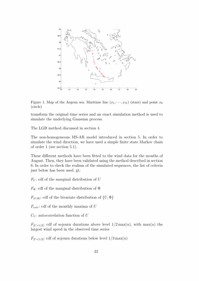
3 years of data (from October 1999 to September 2002) describing the seastate conditions (i.e. (Hs, T,Θm)) at N = 17 points along the maritime line.These points will be denoted (x1, · · · , xN).

11 years (from January 1992 to December 2002) of wind data at a pointdenoted x0, located near the middle of the maritime line (see 1)

The sea state data have been produced using the WAM model by the NationalCenter for Marine Research (NCMR), and the wind data are reanalysis dataproduced by ECMWF. The amount of sea state data is clearly to small inorder to get reliable estimates of the variability of the sea state conditions,and thus we have proposed to use a stochastic generator. In (Ailliot et al.,2003), this sea state generator is combined with a crossing simulator. Thiscrossing simulator is based on polar diagrams which describe the response ofthe passenger ship under consideration in different conditions. These diagramspermit to compute, according to the sea state conditions on the maritimeline, if the crossing can be done in normal conditions, or has to be delayed orcanceled. And as a final result, we can deduce estimates of the distribution ofcanceled and delayed crossings. In this paper, we will only focus on the seastate generator.

The Piraeus-Heraklion line is located in Aegean Sea, which is a relatively closedsea. Thus we can consider that the waves are essentially generated by localwinds and it seems natural to perform the simulation in two steps. At first, astochastic model is used to simulate artificial wind conditions at x0, and thenthe sea state conditions corresponding to these artificial wind conditions arecross-reconstructed. These two steps are described more precisely hereafter.

Simulation of artificial wind conditions

In order to simulate artificial wind conditions at x0, we have tried three dif-ferent methods: gt;

The TGP method discussed in section 3. The transformation (4) is used to

21

20 21 22 23 24 25 26 27 28 2934.5

35

35.5

36

36.5

37

37.5

38

38.5

39

Figure 1. Map of the Aegean sea. Maritime line (x1, · · · , xN ) (stars) and point x0

(circle)

transform the original time series and an exact simulation method is used tosimulate the underlying Gaussian process.

The LGB method discussed in section 4.

The non-homogeneous MS-AR model introduced in section 5. In order tosimulate the wind direction, we have used a simple finite state Markov chainof order 1 (see section 5.1).

These different methods have been fitted to the wind data for the months ofAugust. Then, they have been validated using the method described in section6. In order to check the realism of the simulated sequences, the list of criteriajust below has been used. gt;

FU : cdf of the marginal distribution of U

FΦ: cdf of the marginal distribution of Φ

F(U,Φ): cdf of the bivariate distribution of U,Φ

Fextr: cdf of the monthly maxima of U

CU : autocorrelation function of U

F[U>1/2]: cdf of sojourn durations above level 1/2 max(u), with max(u) thelargest wind speed in the observed time series

F[U<1/3]: cdf of sojourn durations below level 1/3 max(u)

22

The cdf FU , FΦ and F(U,Φ) are important criteria since the distribution of thewind is strongly related to the distribution of the sea state parameters. Fextr

describes the interannual variability of the process at a monthly scale. Theautocorrelation function CU is a usual measure of linear dependence in time.Finally, the cdf of sojourn durations F[Y >1/2] and F[Y <1/3] describe the timeduration of the stormy and calm conditions. These durations are also stronglyrelated to the severity of the sea state conditions.

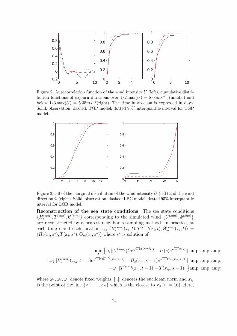
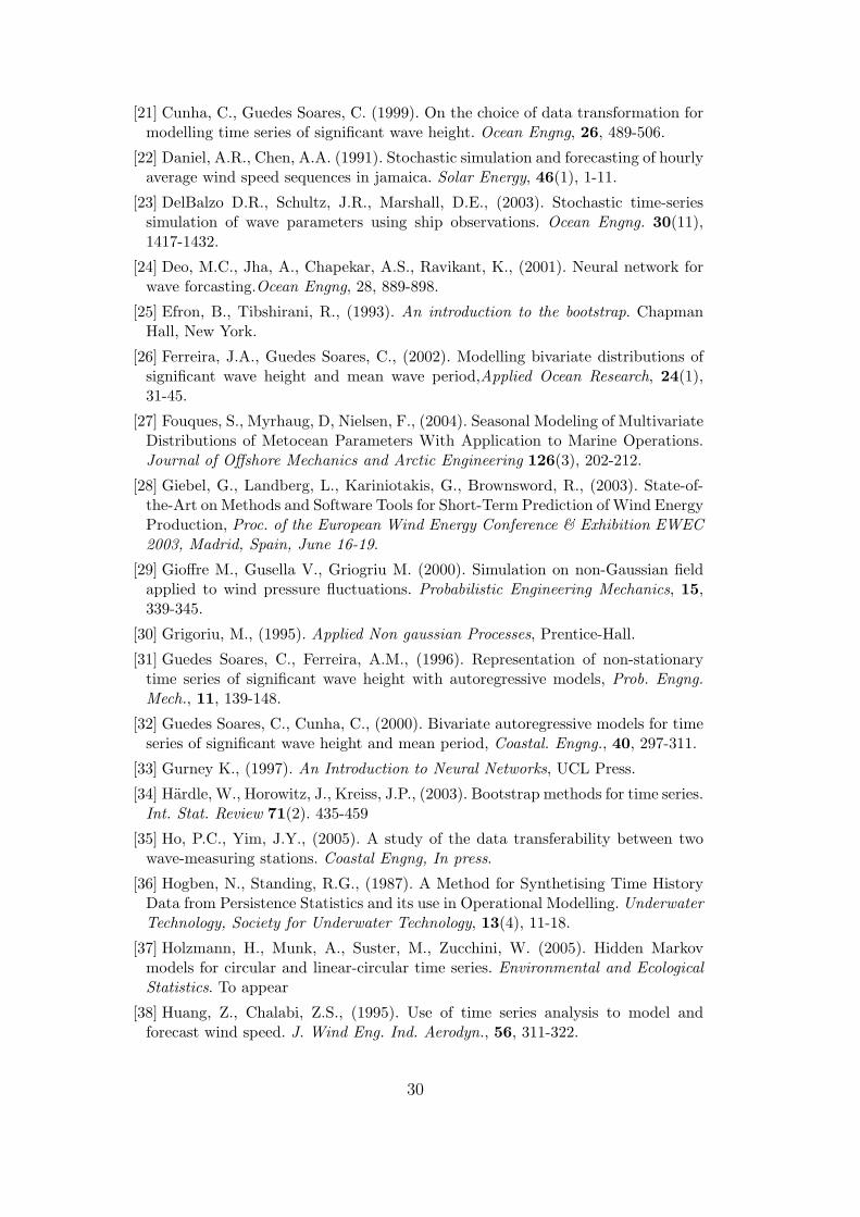
For each criteria, Monte Carlo tests have been run on the basis of N = 1000synthetic time series, each of them having the same length as the initial windtime series. The results are given in Table 1. According to this table, theTGP method successfully reproduces the bivariate marginal distribution ofthe process but fails to reproduce its dynamics. This is also illustrated onFigure 2. According to this figure, the model underestimates the first coeffi-cients of the autocorrelation function and also the durations of the calm andstormy periods. It indicates that the transformed time series is not Gaussian,although its bivariate marginal distribution is Gaussian. On the opposite, theLGB method successfully describes the dynamics of the process but can notrestore the marginal distribution of U and (U,Φ). According to Figure 3 thismethod simulates too many data close to the mode of the distributions. It isa well known problem of this kind of algorithm, and better results could per-haps be obtained with an other choice of the bandwidth parameters. However,the search of appropriate parameters is fastidious since there is no automaticcriterion. As concerns the non-homogeneous MS-AR model, the model withM = 2 regimes and autoregressive models of order p = 1 has been selectedwith BIC, and the results obtained with this model are better than the onescorresponding to LGB and TGP. Indeed, this model reproduces all the cri-teria, except the bivariate marginal distribution. According to Figure 4, themodel simulates too many wind from the north-west and not enough from thenorth, but the distribution of the wind intensity in each sector seems to be wellreproduced. A better description of this bivariate distribution could probablybeen obtained by using a more sophisticated model for the wind direction anda higher number of regimes.

An other advantage of this model over the other models considered in thissection is its physical interpretability. The maximum likelihood estimates aregiven in Table 2. According to this table, one important difference betweenthe two regimes is the value of the conditional standard deviation σ, which ishigher in the second regime. It indicates that the second regime is associatedto weather conditions in which the wind speed evolves quickly, whereas thefirst regime corresponds to steady wind speed conditions (low volatility). Thisis illustrated on Figure 5. And the two regimes are associated to different winddirections (see Figure 6), the first one corresponding mainly to Northerlies andthe second one to Westerlies. This relation is described through the parametersφ and κ.

23

0 5 10−0.2

0

0.2

0.4

0.6

0.8

0 2 40

0.2

0.4

0.6

0.8

1

0 5 100

0.2

0.4

0.6

0.8

1

Figure 2. Autocorrelation function of the wind intensity U (left), cumulative distri-bution functions of sojourn durations over 1/2 max(U) = 8.05ms−1 (middle) andbelow 1/3 max(U) = 5.35ms−1(right). The time in abscissa is expressed in days.Solid: observation, dashed: TGP model, dotted 95% interquantile interval for TGPmodel.

2 4 6 8 10 120

0.2

0.4

0.6

0.8

1

N E S W N0

0.2

0.4

0.6

0.8

1

Figure 3. cdf of the marginal distribution of the wind intensity U (left) and the winddirection Φ (right). Solid: observation, dashed: LBG model, dotted 95% interquantileinterval for LGB model.

Reconstruction of the sea state conditions The sea state conditionsH(sim)

s , T (sim),Θ(sim)m corresponding to the simulated wind U (sim),Φ(sim)

are reconstructed by a nearest neighbor resampling method. In practice, ateach time t and each location xi, (H(sim)

s (xi, t), T(sim)(xi, t),Θ

(sim)m (xi, t)) =

(Hs(xi, s∗), T (xi, s

∗),Θm(xi, s∗)) where s∗ is solution of

mins

ω1||U (sim)(t)e√−1Φ(sim)(t) − U(s)e

√−1Φ(s)|| amp; amp; amp;

+ω2||H(sim)s (xi0 , t− 1)e

√−1Θ

(sim)m (xi0

,t−1) −Hs(xi0 , s− 1)e√−1Θm(xi0

,s−1)||amp; amp; amp;

+ω3||T (sim)(xi0 , t− 1) − T (xi0 , s− 1)||

amp; amp; amp;

where ω1, ω2, ω3 denote fixed weights, ||.|| denotes the euclidean norm and xi0

is the point of the line x1, · · · , xN which is the closest to x0 (i0 = 16). Here,

24

5%

15%

25%

E

N

W

S

5%

15%

25%

E

N

W

S

Figure 4. Wind roses for the data (left) and the data simulated with the non homo-geneous MS-AR model (right)

TGP LGB MS-AR

FU .282 [.003] .000 [.001] 0.078 [.005]

FΦ .003 [.000] .001 [.000] .004 [.000]

F(U,Φ) 0.210 [.001] .000 [.001] .000 [.001]

Fextr .012 [.012] .025 [.009] .137 [.008]

CU .000 [.001] .006 [.003] .001 [.000]

F[U>1/2] .000 [.007] .046 [.006] .015 [.002]

F[U<1/3] .000 [.007] .068 [.002] .042 [.003]

Table 1Results of the Monte Carlo tests for the wind time series. The first value is the

observed statistic wobs and the value in bracket the cut-off value wα with α = 0.05.The null hypothesis is rejected at the level α if wobs < wα

a(i)1 b(i) σ(i) πi,i φ(i) κ(i)

Regime 1 (i=1) 0.85 0.82 1.27 0.96 1.64 1.47

Regime 1 (i=2) 0.53 2.11 2.24 0.95 1.59 2.71

Table 2Maximum likelihood estimates for the non-homogeneous MS-AR model

ω1, ω2, ω3 are chosen empirically.

We have used this simple method to compute the sea-state conditions corre-sponding to the artificial wind conditions simulated with the non homogeneousMS-AR model. Then, in order to check the realism of these artificial sea stateconditions, we have performed Monte Carlo tests, and the list of criteria just

25

0 5 10 15 20 25 30 350

5

10

15

Figure 5. Evolution of the wind speed at x0 in August 2002. The dash-dotted [resp.solid] line represents the date when the first [resp. second] regime is the most likely.The regimes have been identified using the Viterbi algorithm

Figure 6. Distribution of the wind direction in the two regimes (identified using theViterbi algorithm). Regime 1 on the left and regime 2 on the right.

below has been used.

gt;

FHs: cdf of the marginal distribution of Hs

FΘm: cdf of the marginal distribution of Θm

FT : cdf of the marginal distribution of T

F(Hs,Θm): cdf of the bivariate marginal distribution of (Hs,Θm)

F(Hs,T ): cdf of the bivariate marginal distribution of (Hs, T )

F(U,Hs): cdf of the bivariate marginal distribution of (U,Hs)

CHs: autocorrelation function of Hs

F[Hs>1/2] : cdf of sojourn durations above level 1/2 max(Hs)

26

F[Hs<1/3]: cdf of sojourn durations below level 1/3 max(u)

Table 3 shows that all the considered statistics are well reproduced at location16 (located near the middle of the maritime line), except the marginal distri-butions of Θm and (Hs,Θm). This bivariate distribution is shown on Figure 7and the lack of fit is in accordance to the one identified on the simulated windtime series: the proportion of wave coming from the north is underestimated.The joint distribution of U and Hs is shown on Figure 8.

FHsFΘm

FT F(Hs,Θm) F(Hs,T )

.007 [.004] .000 [.002] .017 [.011] .000 [.001] .017[.011]

F(U,Hs) CHsF[Hs>1/2] F[Hs<1/3]

.027 [.005] .024 [.001] .011 [.001] .031 [.005]

Table 3Results of the Monte Carlo tests for the sea state time series at location 16. The

first value is the observed statistic wobs and the value in bracket the cut-off valuewα with α = 0.05. The null hypothesis is rejected at the level α if wobs < wα

10%

30%

50%

E

N

W

S

10%

30%

50%

E

N

W

S

Figure 7. Wave roses for the data at location 16 (left) and for the simulated sequences(right)

8 Concluding remarks

In this paper, we make a review of stochastic models for metocean time series.The models are classified in three groups: gt;

non parametric models

models based on Gaussian approximations

other parametric models

27

0 5 100

0.5

1

1.5

0

0.1

0.2

0.3

0.4

0.5

0 5 100

0.5

1

1.5

0

0.1

0.2

0.3

0.4

0.5

Figure 8. Joint distribution of U (x-axis) and Hs (y-axis). Data on the left andmodel on the right

For each group of models, we discuss the possible uses of the models, theiradvantages and drawbacks, etc. Then a quantitative method is proposed tomeasure the ability of a model to restore chosen statistical feature like marginaldistribution, covariance functions, durations, etc., and this method allows tovalidate or compare models for given data. And finally an example is dis-cussed where a stochastic model is used to generate a multivariate time seriesU,Φ, Hs, T,Θm at several location along a ferry line in Aegean Sea (Greece).

Finally, a lot of tools and methods are available for modeling metocean timeseries and the choice of a model depends on the nature of the studied pro-cess (univariate or bivariate, intensity and/or direction, ...), of the consideredlocation and also on the objectives of the users.

The review focus on models for time series at the scale of the sea state. And,as a consequence, we have neglected many usual and interesting aspects ofmetocean studies, such as, for instance, linear and non linear models for waves,extremes, spatial process.

References

[1] Ailliot, P., Prevosto, M., (2001). Two methods for simulating the bivariateprocess of wave height and direction. Proc. of ISOPE Conf., III, 15-18.

[2] Ailliot, P., Prevosto, M., Soukissian, T., Diamanti, C., Theodoulides, A., PolitisC., (2003). Simulation of sea state parameters process to study the profitabilityof a maritime line. Proc. of ISOPE Conf., III, 51-57.

[3] Ailliot, P., (2004). Modeles autoregressifs a changement de regimes markovien -Application a la simulation du vent. PhD Thesis. Universite de Rennes 1.

[4] Ailliot, P., Monbet, V., Prevosto, M., (2006a). An autoregressive model withtime-varying coefficients for wind fields. Environmetrics, 17(2), 107-117.

28

[5] Ailliot, P., Frenod, E., Monbet, V. (2006b). Long term object drift forecast inthe ocean with tide and wind. To appear in Multiscale Modeling and Simulation.

[6] Arena, F., Puca, S., (2004). The reconstruction of significant wave height timeseries by using a neural network approach. J. Offshore Mechanics and Artic Eng.,126(3), 213-219.

[7] Athanassoulis, G.A., Skarsoulis, E.K., Belibassakis, K.A., (1994). Bivariatedistributions with given marginals with an application to wave climate description.Applied Ocean Research, 16(1), 1-26.

[8] Athanassoulis, G.A., Belibassakis, K.A., (2002). Probabilistic description ofmetocean parameters by means of kernel density models. 1. theoritical backgroundand first results. Appl. Oc. Research 24, 1-20.

[9] Athanassoulis, G.A., Stephanakos, C.N., (1995). A nonstationary stochasticmodel for long-term time series of significant wave height. Journal of GeophysicalResearch, Section Oceans 100(C8), 14149-14162.

[10] Baxevani and I. Rychlik (2004). Fatigue Life Prediction for a Vessel Sailing theNorth Atlantic Route. Proc. ISOPE PACOMS .

[11] Berchtold, A. and Raftery, A.E. (2002). The Mixture Transition Distribution(MTD) model for high-order Markov chains and non-Gaussian time series.Statistical Science,17, 328-356.

[12] Borgman L.E., Sheffner N.W. (1991). Simulation of time sequences of waveheight, period and direction. Technical report US Army Corps of Engineers.

[13] Boukhanovksy, A., Lavrenov, I., Lopatoukhin, L., Rozhnov, V., Divinsky, B.,Kosyan, R., Abdalla, S., Ozhan, E., (1999). Persistence statistics for Balck andBaltic seas. Proc. of Int. MEDCOAST conf. ”Wind and Wave climate, 99”, 199-210.

[14] Box, G.E.P., Jenkins, G.M., (1976). Time series analysis, forecasting andcontrol. (revised edn.) Holden-Day, San Francisco.

[15] Breckling, J. (1989). The Analysis of Directional Time Series. Lecture Notes inStatistics Series.

[16] Brockwell, P., Davis, R., (1991). Time series: theory and methods, 2nd edition.Springer Verlag, New York.

[17] Brown, B.G., Katz, R.W, Murphy, A.H. (1984). Time series models to simulateand forecast wind speed and wind power. J. of clim. and appl. meteor. 23, 1184-1195.

[18] Buishand, T.A., Brandsma, T., (2001). Multi-site simulation of dailyprecipitation and temperature in the Rhine basin by nearest-neighbor resampling.Water Resources Research, 37, 2761-2776.

[19] Caires, S., Sterl, A., (2005). A new non-parametric method to correct modeldata: Application to significant wave height from the ERA-40 reanalysis. J.Atmospheric and Oceanic Tech., In press.

[20] Castino, F., Festa, R., Ratto, C.F. (1998). Stochastic modelling of windvelocities time series, J. of Wind Engineering & Industrial Aerodynamics, 74-76,141-151.

29

[21] Cunha, C., Guedes Soares, C. (1999). On the choice of data transformation formodelling time series of significant wave height. Ocean Engng, 26, 489-506.

[22] Daniel, A.R., Chen, A.A. (1991). Stochastic simulation and forecasting of hourlyaverage wind speed sequences in jamaica. Solar Energy, 46(1), 1-11.

[23] DelBalzo D.R., Schultz, J.R., Marshall, D.E., (2003). Stochastic time-seriessimulation of wave parameters using ship observations. Ocean Engng. 30(11),1417-1432.

[24] Deo, M.C., Jha, A., Chapekar, A.S., Ravikant, K., (2001). Neural network forwave forcasting.Ocean Engng, 28, 889-898.

[25] Efron, B., Tibshirani, R., (1993). An introduction to the bootstrap. ChapmanHall, New York.

[26] Ferreira, J.A., Guedes Soares, C., (2002). Modelling bivariate distributions ofsignificant wave height and mean wave period,Applied Ocean Research, 24(1),31-45.

[27] Fouques, S., Myrhaug, D, Nielsen, F., (2004). Seasonal Modeling of MultivariateDistributions of Metocean Parameters With Application to Marine Operations.Journal of Offshore Mechanics and Arctic Engineering 126(3), 202-212.

[28] Giebel, G., Landberg, L., Kariniotakis, G., Brownsword, R., (2003). State-of-the-Art on Methods and Software Tools for Short-Term Prediction of Wind EnergyProduction, Proc. of the European Wind Energy Conference & Exhibition EWEC2003, Madrid, Spain, June 16-19.

[29] Gioffre M., Gusella V., Griogriu M. (2000). Simulation on non-Gaussian fieldapplied to wind pressure fluctuations. Probabilistic Engineering Mechanics, 15,339-345.

[30] Grigoriu, M., (1995). Applied Non gaussian Processes, Prentice-Hall.

[31] Guedes Soares, C., Ferreira, A.M., (1996). Representation of non-stationarytime series of significant wave height with autoregressive models, Prob. Engng.Mech., 11, 139-148.

[32] Guedes Soares, C., Cunha, C., (2000). Bivariate autoregressive models for timeseries of significant wave height and mean period, Coastal. Engng., 40, 297-311.

[33] Gurney K., (1997). An Introduction to Neural Networks, UCL Press.

[34] Hardle, W., Horowitz, J., Kreiss, J.P., (2003). Bootstrap methods for time series.Int. Stat. Review 71(2). 435-459

[35] Ho, P.C., Yim, J.Y., (2005). A study of the data transferability between twowave-measuring stations. Coastal Engng, In press.

[36] Hogben, N., Standing, R.G., (1987). A Method for Synthetising Time HistoryData from Persistence Statistics and its use in Operational Modelling. UnderwaterTechnology, Society for Underwater Technology, 13(4), 11-18.

[37] Holzmann, H., Munk, A., Suster, M., Zucchini, W. (2005). Hidden Markovmodels for circular and linear-circular time series. Environmental and EcologicalStatistics. To appear

[38] Huang, Z., Chalabi, Z.S., (1995). Use of time series analysis to model andforecast wind speed. J. Wind Eng. Ind. Aerodyn., 56, 311-322.

30

[39] IAHR, (1989). List of sea state parameters, J. Waterway Port Coast. Ocean.Eng., 115 (6), 793-808.

[40] Izquierdo, P., Guedes Soares, C., (2005). Analysis of sea waves and wind fromX-band radar. Ocean Engineering, 32(11-12), 1404-1419.

[41] Jenkins, A.D., (2002). Wave duration/persistence statistics, recording interval,and fractal dimension. International Journal of Offshore and Polar Engineering,12(2), 109-113. 2002

[42] Lahiri, S.N. (2003). Resampling Methods for Dependent data, Springer, NewYork.

[43] Lall, U., Sharma, A., (1996). A nearest neighbor bootstrap for resamplinghydrologic time series. Water Ressources Res., 32, 679-693.

[44] MacDonald, I. L., Zucchini W., (1997). Hidden Markov and Other Models forDiscrete-Valued Time Series. New York: Chapman and Hall.

[45] Makarynskyy, O., Pires-Silva, D., Makarynska, D., Ventura-Soares, C., (2004).Artificial neural networks in wave prediction at the west coast of Portugal,Computer & Geosciences, In press

[46] Marteau, P.F., Monbet, V., Ailliot, P., (2004a). Non parametric modeling ofcyclo-stationary markovian processes - part 2. Proc. ISOPE Conf., III, 145-151.

[47] Marteau, P.F., Monbet, V., (2004b). Conditional prediction of Markovprocesses using non parametric Viterbi algorithm - Comparison with MLP andGRNNmodels, WSEAS Trans. on systems, 3(2), 346-351.

[48] Medina, J.R., Gimenez, M.H., Hudspeth, R.T., (1991). A wave climatesimulator. Proc. 24th Int. Ass. Hydrolic Res. Congress, 521-528.

[49] Monbet, V., Prevosto, M., (2001a). Bivariate Simulation of Non Stationary andNon Gaussian Observed Processes . Application to Sea State Parameters. AppliedOcean Research, 23, 139-145.

[50] Monbet V., Marteau P.F., (2001b). Continuous Space Discrete Time MarkovModels for Multivariate Sea State Parameter Processes. Proc. ISOPE Conf., III,10-14.

[51] Monbet V., Marteau P.F., (2004). Non parametric modeling of cyclo-stationarymarkovian processes. Proc. ISOPE Conf., III, 138-144.

[52] Monbet V., Marteau P.F., (2005a). The Local Grid Bootstrap for StationaryMultivariate Markov Processes, J. Statistical Planning and Inference, in press.

[53] Monbet V., Ailliot P., (2005b). L1-convergence of smoothing densitiesin non parametric state space models submitted to Stat. Inf. for Stoch. Proc.

[54] More, A., Deo, M.C., (2003). Forecasting wind with neural networks. Marinestructures, 16 , 35-49.

[55] Nfaoui, H., Buret, J., Sayigh, A.A., (1996). Stochastic simulation of hourlyaverage wind speed sequences in Tangiers (Morocco). Solar Energy, 56(3), 301-314.

[56] O’Carroll, (1984). Weather Modelling for Offshore Operations. The Statistician,33, pp 161-169.

31

[57] Pittalis, S., Bruschi, A., Puca, S., Tirozzi, B., (2003). Reconstruction of seaevents and extreme value analysis. Proc. ISOPE Conf., III.

[58] Poggi, P., Muselli, M., Notton, G., Cristofari, C., Louche, A., (2003). Forcastingand simulating wind speed in Corsica by using an autoregressive model. Energyconversion and management, 44, 3177-3196.

[59] Popescu, R., Deodatis, G., Prevost, J.H. (1998). Simulation of homogeneousnonGaussian stochastic vector fields. Prob. Engng. Mech, 13(1), 1-13.

[60] Raftery, A.E., (1985). A model for higher-order Markov chains. J. Roy. Statist.Soc. Ser. B, 47, 528-539.

[61] Raftery, A.E., Tavare, S. (1994). Estimation and modelling repeated patterns inhigh-order Markov chains with the mixture transition distribution (MTD) model.J. Roy. Statist. Soc. Ser. C - Applied Statistics, 43, 179-200.

[62] Rychlik, I., Johannesson, P., Leadbetter, M.R., (1997). Modelling an dstatisticalanalysis of ocean-wave data using transformed Gaussian processes. MarineStructures. 10, 13-47.

[63] Scotto, M.G., Guedes Soares, C., (2000). Modelling the long-term time seriesof significant wave height with non linear threshold models. Coastal Engng, 40,313-327.

[64] Shi S.G., (1991). Local Bootstrap. Ann. Institut. Statist. Math., 43, 667-676.

[65] Soukissian, T., Theochari, Z., (2001). Joint occurrence of sea states andassociated durations, Proc. ISOPE Conf., III, 33-39.

[66] Stefanakos, C.N., (1999). Nonstationary stochastic modelling of time series withapplications to environmental data. PhD Thesis. NTAU.

[67] Stefanakos, C.N., Athanassoulis, G.A., (2001). A unified methodology for theanalysis, completion and simulation of nonstationary time series with missing-values, with application to wave data. Applied Ocean Research, 23(4), 207-220.

[68] Stefanakos, C.N., Athanassoulis, G.A., Barstow, S.F., (2002), Multiscale TimeSeries Modelling of Significant Wave Height. Proc. ISOPE Conf., vol. III, pp66-73.

[69] Stefanakos, C.N., Belibassakis, K.A., (2005). Nonstationary StochasticModelling Of Multivariate Long-term Wind And Wave Data, 24th Int. Conf. onOffshore Mechanics and Arctic Engineering, OMAE’2005.

[70] Stephos, A., (2000). A comparison of various forecasting techniques applied tomean hourly wind time series. Renewable Energy, 21, 23-35.

[71] Toll, R.S.J., (1997). Autoregressive conditional heteroscedasticity in dayly windspeed measurements, Theor. Appl. Climatol., 56, 113-122.

[72] Tsai, C.P., Lin, C., Shen, J.N., (2002). Neural network for wave forcastingamoung multi-stations, Ocean Engineering, 29, 1683-1695.

[73] Turlach, B.A., (1993). Bandwidth selection in kernel density estimation: areview. Techn. report.

[74] Vanhoff, B., Elgar, S., (1997). Numericallu simulation non-Gaussian seasurfaces, J. of Waterway, Port, Coastal and Ocean Engng, 124, 68-72.

32

[75] Vik, I. (1981). The tile series generating module-Modelling aspects OceanResearch- operational criteria, CNRD 3-2 task 2.

[76] Waeles, B., Le Hir P., Silva Jacinto R. (2004). Modelisation morphodynamiquecross-shore d’un estran vaseux. C. R. Geoscience, 336, 1025-1033.

[77] Walton, T.L., Borgman, L.E. (1990). Simulation of non-stationary, non-gaussianwater levels on the great lakes, J. of Waterways, Ports, Coastal and OceanDivision, ASCE, 116(6).

[78] Wang, D.W., Hwang P. (2001). An operational method for separating windsea and swell from ocean wave spectra. J. Atmospheric and Oceanic Technology.18(12), 2052-2062.

[79] Woolf, D.K., Challenor, P.G., (2002). Statistical comparison of satellite andmodel waves climatologies, Proc. 4th symp. WAVES

[80] Yim, J.Z., Chou, C., Ho, P., (2002). A study on simulating the time series ofsignificant wave height near the keelung harbor. Proc. ISOPE Conf., vol III.

[81] Young, P.C., NG, C.N., Lane, K., Parker, D., (1991). Recursive forcasting,smoothing and seasonal adjustement of non-stationary environmental data, J.Forecast, 10, 58-89.

[82] Young, K.C., (1994). A multivariate chain model for simulating climaticparameters from daily data, J. Appl. Meteorol., 33, 661-671.

33