Survey Methods & Design in Psychology Lecture 11 (2007) Significance Testing, Power, Effect Sizes,...

Survey Methods & Design in Psychology

Lecture 11 (2007)

Significance Testing, Power,

Effect Sizes, Confidence Intervals, Publication Bias, & Scientific Integrity

Lecturer: James Neill

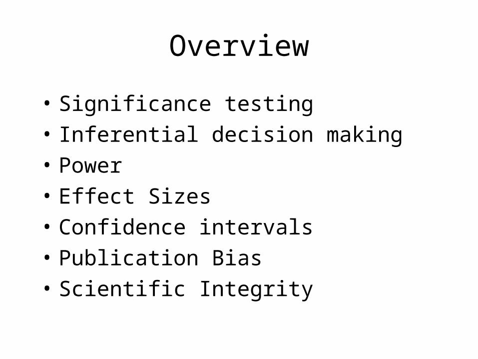
Overview

• Significance testing

• Inferential decision making

• Power

• Effect Sizes

• Confidence intervals

• Publication Bias

• Scientific Integrity

Readings

Howell Statistical Methods:

• Ch8 Power

Concepts rely upon:

• Ch3 The Normal Distribution

• Ch4 Sampling Distributions and Hypothesis Testing

• Ch7 Hypothesis Tests Applied to Means

Significance Testing

Significance Testing

• Logic• History• Criticisms• Hypotheses• Inferential decision making table

– Type I & II errors– Power– Effect Size (ES)– Sample Size (N)

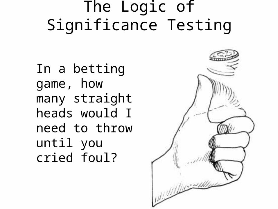
The Logic of Significance Testing

In a betting game, how many straight heads would I need to throw until you cried foul?

The Logic of Significance Testing

Sample Population

• A 20th C phenomenon.

• Developed by Ronald Fisher for testing the variation in produce per acre for agriculture crop (1920’s-1930’s)

History of Significance Testing

• To help determine what agricultural methods (IVs) yielded greater output (plant growth) (DVs)

• Designs couldn’t be fully experimental, therefore, needn’t to determine whether variations in the DV were due to chance or the IV(s).


• Proposed H0 to reflect expected ES in the population

• Then get p-value from data about the likelihood of H0 being true &, depending of level of false positives the researcher is prepared to tolerate (critical alpha), make decision about H0


• ST spread to other fields, including social science

• Spread in use aided by the development of computers and training.

• In the latter decades of the 20th C, widespread use of ST attracted critique for its over-use and mis-use.


• Critiqued as early as 1930

• Cohen (1980’s-1990’s) critiqued

• During the late 1990’s a critical mass of awareness developed and there are currently changes underway in publication criteria and teaching with regard to over-reliance on ST

Criticisms of Significance Testing

• Null hypothesis is rarely true


• NHT only provides a binary decision (yes or no) and indicates the direction

• Mostly we are interested in the size of the effect – i.e., how much of an effect?


• Whether a result is significant is a function of:– ES– N– critical level

• Sig. can be manipulated by tweaking any of the three (as each of them increase, so does the likelihood of a significant result)


Statistical vs Practical Significance

• Statistical significance means that the observed mean differences are not likely due to sampling error

– Can get statistical significance, even with very small population differences, if N is large enough

• Practical significance looks at whether the difference is large enough to be of value in a practical sense

– Is it an effect worth being concerned about – does it have any noticeable or worthwhile effects?

• Logic: Sample data examined to determine likelihood it represents a population of no effect or some effect.

• History: Developed by Fisher for agricultural experiments in early 20th C

• Spread aided by computers to social science• In recent decades, ST has been criticised for

over-use and mis-application.

Significance Testing - Summary

Recommendations

• Learn traditional Fisherian logic methodology (inferential testing)

• Learn alternative techniques (ESs and CIs)

• -> Use ESs and CIs as alternatives or complements to STs.

Recommendations

• APA 5th edition recommends reporting of ESs, power, etc.

• Recognise merits and shortcomings of each approach

• Look for practical significance

Inferential Decision Making

Hypotheses in Inferential Testing

Null Hypothesis (H0): No differences

Alternative Hypothesis (H1): Differences

Inferential Decisions

When we test a hypothesis we draw a conclusion; either

Accept H0p is not significant (i.e. not below the critical )

Reject H0:

p is significant (i.e., below the critical )

Type I & II Errors

When we accept or do not accept H0, we risk making one of two possible errors:

Type I error:Reject H0 when it is actually correct

Type II error:Retain H0 when it is actually false

Correct Decisions

When we accept or do not accept H0, we are hoping to make one of two possible correct decisions:

Correct rejection of H0 (Power):

Reject H0 when there is a real difference

Correct acceptance of H0:

Retain H0 when there is no real difference

Inferential Decision Making Table

• Type I error (false rejection of H0) =

• Type II error (false acceptance of H0) =

• Power (false rejection of H0) = 1-

• Correct acceptance of H0 = 1-

Significance Testing - Summary

Power• The probability of rejection of a false

null-hypothesis• Depends on the:

–Critical alpha ()–Sample size (N) –Effect size (Δ)

Power

= Likelihood that an inferential test will return a sig. result when there is a real difference

= Probability of correctly rejecting H0

= 1 - likelihood that an inferential test won’t return a sig. result when there is a real difference (1 - β)

• Desirable power > .80• Typical power ~ .60

PowerAn inferential test is more ‘powerful’ (i.e.

more likely to get a significant result) when any of these 3 increase:

Power Analysis

• If possible, calculate expected power beforehand, based on:

- Estimated N, - Critical , - Expected or minimum ES

(e.g., from related research)

• Also report actual power in the results.• Ideally, power ~ .80 for detecting small

effect sizes

T

alpha 0.05

Sampling distribution if HA were true

Sampling distribution if H0 were true

POWER: 1 -

Standard Case

Non-centrality parameter

T

alpha 0.05



POWER: 1 - ↑

Increased effect size


Impact of more conservative

T

alpha 0.01Sampling distribution if HA were true


POWER: 1 - ↓


Impact of less conservative

T

alpha 0.10Sampling distribution if HA were true


POWER: 1 - ↑


T

alpha 0.05



POWER: 1 - ↑

Increased sample size


• Power is the likelihood of detecting an effect as statistically significant

• Power can be increased by: N critical ES

• Power over .8 “desirable”• Power of ~.6 is more typical• Can be calculated prospectively and

retrospectively

Power Summary

Effect Sizes

• ESs express the degree or strength of relationship or effect

• Not influenced the N• ESs can be applied to any inferential test, e.g.,

– r for correlational effects– R for multiple correlation effects– d for difference between group means– eta-squared (2) for multivariate differences between

group means

Effect Sizes

Commonly Used Effect Sizes

Standardised Mean difference• Cohen’s d • F / 2

Correlational• r, r2

• R, R2

Cohen’s d

• A standardised measure of the difference between two Ms

• d = M2 – M1 /

Cohen’s d

• Cohen’s d

-ve = negative change

0 = no change

+ve = positive change

Effect sizes – Cohen’s d

• Not readily available in SPSS

• Cohen’s d is the standardized difference between two means

Example Effect Sizes

-5 0 50

0.2

0.4

d=.5-5 0 50

0.2

0.4

d=1

-5 0 50

0.2

0.4

d=2-5 0 50

0.2

0.4

d=4

Group 1

Group 2

• Cohen (1977): .2 = small .5 = moderate .8 = large

• Wolf (1986): .25 = educationally significant

.50 = practically significant (therapeutic)

• Standardised Mean ESs are proportional, e.g., .40 is twice as much change as .20

Interpreting Standardised Mean Differences

Interpreting Effect Size

• No agreed standards for how to interpret an ES

• Interpretation is ultimately subjective

• Best approach is to compare with other studies

• In practice, a small ES can be very impressive if, for example:– the outcome is difficult to change

(e.g. a personality construct) or if – the outcome is very valuable

(e.g. an increase in life expectancy).

• On the other hand, a large ES doesn’t necessarily mean that there is any practical value if it isn’t related to the aims of the investigation (e.g. religious orientation).

A Small Effect Size Can be Impressive…

Graphing Effect Size - Example

Effect Size Table - Example

Effect sizes – Exercise

• 20 athletes rate their personal playing ability, with M = 3.4 (SD = .6) (on a scale of 1 to 5)

• After an intensive training program,the players rate their personal playing ability, with M = 3.8 (SD = .6)

• What is the ES and how good was the intervention?

• What is the 95% CI and what does it indicate?

Effect sizes - Answer

Cohen’s d• = (M2-M1) / SD• = (3.8-3.4) / .6• = .4 / .6• = .67• = a moderate-large change over time

Effect sizes - Answer

Effect sizes - Summary• ES indicates amount of difference or strength

of relationship - underutilised

• Inferential tests should be accompanied by ESs and CIs

• Most common ESs are Cohen’s d and r• Cohen’s d: .2 = small

.5 = moderate

.8 = large

• Cohen’s d is not provided in SPSS – can use a spreadsheet calculator

Power & Effect sizes in Psychology

Ward (2002) examined articles in 3 psych. journals to assess the current status of statistical power and effect size measures.

• Journal of Personality and Social Psychology,

• Journal of Consulting and Clinical Psychology

• Journal of Abnormal Psychology

Power & Effect sizes in Psychology

• 7% of studies estimate or discuss statistical power.

• 30% calculate ES measures.

• A medium ES was discovered as the average ES across studies

• Current research designs do not have sufficient power to detect such an ES.

Confidence Intervals


• Very useful, underutilised

• Gives ‘range of certainty’ or ‘area of confidence’ e.g., true M is 95% likely to lie between -1.96 SD and +1.96 of the sample M

• Based on the M, SD, N, and critical , it is possible to calculate for a M or ES:– Lower-limit– Upper-limit


• Confidence intervals can be reported for:– Ms

– Mean differences (M2 – M1)

– ESs

• CIs can be examined statistically and graphically

Confidence Intervals - Example

Example 1• M = 5, with 95% CI of 2.5 to 7.5• Reject H0 that the M is equal to 0.

Example 2• M = 5, with 95% CI of -.5 to 11.5• Accept H0 that the M is equal to 0.

CIs & Error Bar Graphs

• CIs around means can be presented as error bar graphs

• More informative alternatives to bar graphs or line graphs

• For representing the central tendency and distribution of continuous data for different groups

CIs & Error Bar Graphs


• In addition to getting CIs for Ms, we can obtain and should report CIs for M differences and for ESs.

Independent Samples Test

.764 489 .445 5.401E-02 7.067E-02 -8.48E-02 .1929

.778 355.220 .437 5.401E-02 6.944E-02 -8.26E-02 .1906

t df Sig. (2-tailed)

Mean

Difference

Std. Error

Difference Lower Upper

95% Confidence

Interval of the

Difference

t-test for Equality of Means

Confidence Interval of the Difference

Confidence Interval of a Mean

Program Type

AdolescentsCorporateFamilyAdultsSpecialYoung Adults

Effe

ct S

ize

Tim

e 1

to T

ime

2

.8

.7

.6

.5

.4

.3

.2

Publication Bias, Scientific Integrity, & Cheating

Two counter-acting biases

• Low Power:-> under-estimate of real effects

• Publication Bias or File-drawer effect:-> under-estimate of real effects

Publication Bias

• Occurs when publication of results depends on their nature and direction.

• Studies that show a significant effect are more likely to be published.

• Type I publication errors are underestimated to the extent that they are: “frightening, even calling into question the scientific basis for much published literature.”(Greenwald, 1975, p. 15)

Funnel Plots

• A funnel plot is a scatter plot of treatment effect against a measure of study size.

Risk ratio (mortality)

0.025 1 40

2

1

0S

tan

da

rd e

rro

r

0.25 4

Funnel Plots

Funnel Plots

• Precision in the estimation of the true treatment effect increases as N increases.

• Small studies scatter more widely at the bottom of the graph.

• In the absence of bias the plot should resemble a symmetrical inverted funnel.

Funnel Plots

Publication BiasPublication Bias:

Asymmetrical appearance of the funnel plot with a gap in a bottom corner of the graph

Publication Bias

• In this situation the effect calculated in a meta-analysis will overestimate the treatment effect

• The more pronounced the asymmetry, the more likely it is that the amount of bias will be substantial.

File-drawer Effect

• Tendency for null results to be ‘filed away’ (hidden) and not published.

• No. of null studies which would have to ‘filed away’ in order for a body of significant published effects to be considered doubtful.

Why Most Published Findings are False

Research results are less likely to be true:

1. The smaller the study

2. The smaller the effect sizes

3. The greater the number and the lesser the selection of tested relationships

4. The greater the flexibility in designs

5. The greater the financial and other interests

6. The hotter a scientific field (with more scientific teams involved)

Countering the Bias

Academic Integrity: Students

• N = 954 students enrolled in 12 faculties of 4 Australian universities

• Self-reported:

– Cheating (41%),

– Plagiarism (81%)

– Falsification (25%).

Summary

• Counteracting biases in scientific publishing: – tendency towards low-power studies which

underestimate effects– tendency to publish significant effects over non-

significant effects

• Studies are more likely to draw false conclusions if conducted with small N, ES, many effects, design flexibility, in hotter fields with greater financial interest

• Violations of academic integrity are prevalent, from students through researchers

Recommendations

• Decide on H0 and H1 (1 or 2 tailed)• Calculate power beforehand & adjust the

design to detect a min. ES• Report power, significance, ES and CIs• Compare results with meta-analyses and/or

meaningful benchmarks• Take a balanced, critical approach, striving

for objectivity and scientific integrity

Survey Methods & Design in Psychology Lecture 11 (2007) Significance Testing, Power, Effect Sizes,...

Documents

Transcript of Survey Methods & Design in Psychology Lecture 11 (2007) Significance Testing, Power, Effect Sizes,...