Surface Characterization of Gram-Negative Bacteria and ...599839/FULLTEXT01.pdfGram-negative...
38
Surface Characterization of Gram-Negative Bacteria and their Vesicles Using Fourier Transform Infrared Spectroscopy and Dynamic Light Scattering Sofia Carlsson Degree Thesis in Chemistry 30 ECTS Master’s level Report passed: 07 2012 Supervisors: Madeleine Ramstedt
Transcript of Surface Characterization of Gram-Negative Bacteria and ...599839/FULLTEXT01.pdfGram-negative...

Surface Characterization of Gram-Negative Bacteria and their Vesicles Using Fourier Transform Infrared Spectroscopy and Dynamic Light Scattering
Sofia Carlsson
Degree Thesis in Chemistry 30 ECTS Master’s level Report passed: 07 2012 Supervisors: Madeleine Ramstedt


Abstract
Gram-negative bacteria are known to produce vesicles, why and how is still relatively unknown. Gram-negative bacteria are widely studied but still there are large areas in the field covering the bacterial chemistry that are unknown. This study is a pilot study aimed to complement the studies on surface properties for Gram-negative bacteria and their vesicles. The study is focused on the bacteria Escherichia coli (E.coli). Differences and similarities between bacteria and vesicle surface characteristics and chemical composition are presented using Attenuated Total Reflectance Fourier Transformed Infrared Spectroscopy (ATR-FTIR) and Dynamic Light Scattering (DLS). There does not seem to be any direct correlation between bacteria and vesicles regarding the surface characteristics. However, this study provides interesting data regarding the production of vesicles and vesicle characteristics as well as information regarding the surface characteristics of bacteria.

II
III
List of abbreviations
ε the dielectric constant f (κa) a function of the ratio between the radius of the particle and the
thickness of the electrical double layer. η The viscosity of the solution ATR Attenuated total reflectance D Translational diffusion coefficient DLS Dynamic light scattering DNA Deoxyribonucleic acid E.coli Escherichia coli FTIR Fourier transform infrared Ge Germanium HCl Hydrochloric acid IR Infrared spectroscopy k Boltzmann constant LPS Lipopolysaccharides OM Outer membrane OMP Outer membrane protein OMV Outer membrane vesicle R Hydrodynamic radius of a particle (or molecule) SDS-PAGE Sodium dodecyl sulfate polyacrylamide gel electrophoresis T Absolute temperature TEM Transmission Electron Microscope Z Zeta potential ZnSe Zinc selenide XPS X-ray photoelectron spectroscopy U(E) Electrophoretic mobility

IV
V
Table of contents
Abstract .......................................................................................................................... I List of abbreviations .................................................................................................... III Table of contents ........................................................................................................... V
Why study vesicles from Gram-negative bacteria? ....................................................... 1 Bacteria vs. vesicle ......................................................................................................... 1
Gram-negative bacteria .............................................................................................. 1 Vesicles ...................................................................................................................... 2
Techniques used for analysis ......................................................................................... 4 Infrared (IR) spectroscopy ......................................................................................... 4 Fourier Transformed Infrared (FTIR) Spectroscopy ................................................. 5 Attenuated Total Reflectance (ATR) ......................................................................... 5 Microbial cells ........................................................................................................... 6 Dynamic light scattering, DLS .................................................................................. 6
Size measurement .................................................................................................. 6 Zeta potential measurements .................................................................................. 7
Method ........................................................................................................................... 9 Samples ...................................................................................................................... 9 Buffer preparation .................................................................................................... 10 Preparation of bacteria ............................................................................................. 10 Preparation of outer membrane vesicles .................................................................. 10
Sodium dodecyl sulfate polyacrylamideb gel electrophoresis (SDS-PAGE) ...... 10 DLS analysis ............................................................................................................ 10 ATR-FTIR spectroscopic analysis ........................................................................... 11
Results and discussion ................................................................................................. 11 Optimization of the method ..................................................................................... 11 DLS analyses ........................................................................................................... 14 ATR-FTIR spectroscopic analysis ........................................................................... 17 Other data ................................................................................................................. 23
SDS-PAGE .......................................................................................................... 24 X-ray photoelectron spectroscopy, XPS .............................................................. 24
Conclusions .................................................................................................................. 26 Acknowledgement ....................................................................................................... 26 Bibliography ................................................................................................................ 28

VI
1
Why study vesicles from Gram-negative bacteria?
So far little is known about the outer membrane vesicles (OMV) emerging from the cell surface. Why are they produced, how do they interact and what are their characteristics? There are many theories and studies but so far few answers (1), (2), (3), (4), (5). This study tries to give some answers regarding the surface of vesicles compared to the surface of bacteria. Are there some similarities? Are the characteristics of vesicle surfaces consistent or random? And if similar to bacteria, can we use them to further explore the bacterial surface and its interaction with its surroundings? So why do we want to explore the surface of bacteria? Due to its direct contact with the external environment bacteria are in need of a cell surface that is adaptable to rapid changes in, for example, environmental components, osmotic pressure and nutrients. But it still needs to be strong and stable to survive different kinds of threats (1). This need combined with flexibility have developed unique cell surface properties where still much is unknown. A greater extent of knowledge could develop the usage of bacteria and enable the usage of bacterial vesicles, for example, in the delivery of different drugs to target cells (1). The focus of our research is to gain a greater knowledge of the characteristics of the bacterial surface in the purpose to reach a more comprehensive understanding of bacterial adhesion.
Bacteria vs. vesicle
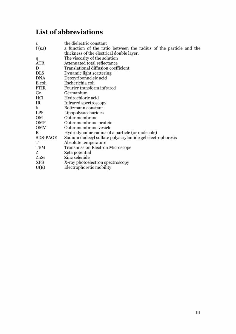
Gram-negative bacteria A Gram-negative bacterium differs from a Gram-positive bacterium mainly when it comes to the outer membrane (OM) and the periplasm which are both missing in the Gram-positive bacteria. The OM consists of lipopolysaccharides (LPS), phospholipids and outer membrane proteins (OMPs). The phospholipids form a bilayer structure where the LPS are attached to the outer leaflet. This structure gives the OM a hydrophilic outer surface and a hydrophobic core. The OMPs forms hydrophilic pores that can act as a link, or channel, between the periplasm and the external environment (1). The periplasm is a macromolecular gel consisting of peptidoglycan and includes periplasmic proteins and other macromolecules. It has a high, fixed polyelectrolyte concentration which makes it isosmotic with the cytoplasmic membrane (1). The outline of Gram-Negative cell wall can be seen in Figure 1 (1).
Figure 1. Schematic image of Gram-negative bacteria.

2
Bacteria are very small organisms with a size range in microns; the size varies between different species. If looking at the transmission electron microscope (TEM) image, Figure 2, it can be seen that E.coli mutant ∆waaG has a size of approximately 1.0-1.5µm. Furthermore, due to this small size, bacteria have a very high surface to volume ratio, approximately 100 000 times (6). The high surface to volume ratio indicates that the membranes of the bacteria is a large contributing factor to the dry mass of the bacteria and understanding this part of the cell should therefore contribute greatly, to the complete understanding of cellular function and -interaction. From previous studies it seems that bacterial size and shape of the cells as well as the buoyant density differ during the growth, they all seem to increase in the exponential phase. However, the zeta potential seems to be constant (7). This indication is reinforced if looking at E.coli bacteria in a TEM. Figure 2a shows an E.coli bacterium that probably is in the beginning of the exponential phase, prior to cell division. This can be compared to Figure 2b that shows a mutant of Pseudomonas aeruginosa that is just about to divide.
a b Figure 2.TEM image of E.coli (a) and Pseudomonas aeruginosa (b). In the red circle in image (a) there is a bacterium in the exponential phase, prior to cell division. In the red circle in image (b) there is a bacterium in the exponential phase during cell division (8).
Vesicles Gram-negative bacteria naturally produce OMVs; small closed bubbles released from the bacteria surface. They are suggested to be formed as a bulge arising from the outer membrane as can be seen in Figure 3 (2), (3). The surface of OMVs are suggested to consist of bacterial outer membrane including LPS and OMPs and it is proposed that they are filled with periplasmic components such as proteins, enzymes and toxins (3), (9). The full mechanism of vesicle production and its components are still not fully understood. In electron microscope they appear as spherical structures with a diameter of 50-250 nm depending on strain (2), (3). It is noteworthy that vesicles are only produced by live bacteria (3).

3
Figure 3. Formation of membrane vesicles.
The purpose of vesicle production is still not fully understood although they seem to be used as transport vehicles for Gram-negative bacteria components to eukaryotic and prokaryotic cells in the surrounding environment of the bacteria (2). They are suggested to function as both a channel of waste handling as well as a delivery system. The range of components that the OMVs are suggested to transport is very broad including virulence factors, antimicrobial agents, DNA, toxins, proteins, antibiotics etc. (3). It seems the components transported can be either fully functional substances with a purpose and/or a target cell or waste material such as missfolded proteins (4). It also seems they can act as virulence factors, carrying substances that damage the target cell in different ways (3). One of the advantages suggested for vesicle production is the possibility to reach host cells located deep in tissues that cannot be reached by the bacteria themselves (2). Vesiculation seems to occur in various environments such as solid or liquid cultures, in biofilms, planktonic cultures as well as natural environments (2), (3), (4). This also includes infected tissues (5). Approximately 1 % of the OM materials in a culture of E.coli are vesicles (5). Interaction of Gram-negative OMVs with bacteria is suggested to occur by attachment to the membrane via adherence or fusion (5). After adherence the vesicles can be internalized into the host cell (5). For Gram-negative bacteria, this is quite a straight forward process that does not need complete reorganization of the outer membrane due to the fact that the OMVs are made of the outer membrane and consist of similar components as the bacterial cell wall (3). When fused into the membrane, the content of the vesicle can be delivered directly into the periplasm of the bacteria (3). The interaction mechanism between Gram-negative OMVs and Gram-positive bacteria is still unknown (3). Due to the fact that the mechanism, composition and production of vesicles are so unknown, there are a number of theories regarding vesiculation although they are not fully comprehensive and restricted to a few species of bacteria. Regarding surface characterization there has been studies on Pseudomonas aeruginosa suggesting that the growth phase of bacteria only affects the zeta

4
potential of the vesicles produced, giving a more negative zeta potential for vesicles when the bacteria are in the stationary phase. The size and the shape are suggested to remain constant (7). Studies, presented in this report, on E.coli vesicles will complement earlier findings in this field. Other interesting studies suggest that there are also differences in the inner content of the vesicles depending on when the vesicles are produced. For example, it is suggested that vesicles produced in the exponential growth phase have a higher amount of proteins (7). It was also suggested that the vesicles produced in the exponential phase have a higher density and are more translucent (7). The amount vesicle produced is suggested to be affected by the charge of the LPS of the bacteria (3), (9) and the rate is suggested to be dependent on the bacterial growth phase with a maximum rate during the late exponential phase (2), (4). All of these things are tested on other bacterial stains than E.coli and they will not be directly studied in the scope of this project. Moreover, early studies made the assumption that the surface charge of bacteria were homogeneously distributed over the surface although newer studies indicates that in reality there is a higher concentration of surface sites at the poles of the bacteria (10). If so, and if vesicles are produced as suggested than there will most likely be a difference in vesicle structure due to where on the bacterial surface it is spun off from. This topic is also outside the scope of this project.
Techniques used for analysis
Infrared (IR) spectroscopy Each atom and each molecule has a motional freedom of three i.e. in x, y and z direction. These motional freedoms can be divided into three different kinds of movements; translational, rotational and vibrational as can be seen in Table 1. The vibrational mode of motional freedom is often referred to as the normal mode of vibration (11), (12). Table 1. Motional freedoms of molecules. N stands for numbers of atoms (11), (12).
Types of degrees of freedom
Linear molecule Non-linear molecule
Translational 3 3 Rotational 2 3 Vibrational 3N-5 3N-6 Total 3N 3N Furthermore, the vibrational modes can then be divided into stretching (change in bond length) and bending modes (change in bond angle). The stretching can be divided into symmetric (in-phase) or asymmetric (out-of-phase) stretching. Moreover, the bending modes can be divided according to type of bending; scissoring, rocking, wagging and twisting. In addition, they can also be divided into in-plane (scissoring and rocking) or out-of-plane (wagging and twisting) (11), (12). The theory behind IR spectroscopy is based on the vibrational modes of motional freedom of the atoms in a molecule and how these vibrations will affect neighboring atoms through chemical bonds (12). However, not all vibrations give rise to an IR spectrum, the vibration has to create a change in the dipole moment of the molecule. The larger the change, the more intense will the absorption bands be (11). A spectrum is obtained by letting infrared radiation pass through the sample and then measuring which fraction of the incident radiation is absorbed at a specific energy (11). Due to the vibrations different substances will absorb different amount of

5
radiation in different regions giving rise to individual spectra that give us information regarding the bonds within a molecule (11). The main advantage of IR spectroscopy is that almost any sample in almost any state can be analyzed with different techniques (11). However, there is one special feature that the analyzed samples have to possess namely, the molecule has to have an electrical dipole moment that changes during vibration (11). An IR spectrum is obtained when a sample absorbs radiation in the region of infrared electromagnetic radiation (400-4000 cm-1 for mid-infrared). When the radiation is absorbed, a quantum mechanical transition occurs between two vibrational energy levels (the ground level and the first excited level for mid-infrared). The difference in energy is directly related to the frequency of the radiation (12).
Fourier Transformed Infrared (FTIR) Spectroscopy The basic idea behind the FTIR spectroscopy is that the inference between two beams of radiation will yield an interferogram; a function of the change of path length between the two beams. This information is then transformed by a mathematical method called Fourier-transformation. The basic outline of the method can be seen in Figure 4. The main advantage of FTIR spectroscopy is that the sample is scanned with the whole spectral range at each time (12).
Figure 4. Basic outline for FTIR spectroscopy.
The crucial part in this setup is the interferometer, where the Michelson interferometer is the most common one. It consists of two mirrors, one fixed and one moveable, and a beam-splitter. The two mirrors are positioned 90 ° angle from each other. The radiation hits the beam-splitter and then 50 % of the beam goes to each mirror. The mirrors reflect the beams back to the beam splitter where they recombine and interfere; this beam is called the transmitted beam and is the one detected by the FTIR spectroscopy (12), (11). The moving mirror will create an optical path difference between the two mirrors. If both mirrors are at the same position they will reflect both beams to the detector. During these conditions, the beams will be in phase when they hit the detector, creating a perfect constructive interference and the radiation signal will be at maximum intensity (12). If not at the same position, there will be an interference pattern created by the difference in optical path length between the two mirrors (11). During each scan the sample will absorb some radiation, lowering the intensity of the incident radiation (12). The second mirror is moved between each scan giving rise to a different interference pattern each time. It is these interference pattern that give rise to the raw data, also called interferogram, that are transformed by the mathematical algorithm Fourier transformation (12).
Attenuated Total Reflectance (ATR) Different reflectance methods are used when the samples are too difficult to analyze using normal transmittance methods. For ATR the sample is placed on a crystal and then radiated with a beam of IR light. The method is based on total internal reflection i.e. an optical phenomenon where, if the incoming angle of radiation is bigger than the critical angle, all light is reflected. The critical angle is a function of the refractive indices of the crystal surfaces (11). A schematic image of the ATR setup can be seen in Figure 5.
Source Interfero-meter Sample Detector Amplifier
Analog-to dogital
converterComputer

6
The crystal used is of materials that have low solubility in water and have high reflective index. This includes for example zinc selenide (ZnSe) and Germanium (Ge) (11).
Figure 5. Example of an ATR setup.
Microbial cells When analyzing microbial cells like bacteria using IR spectroscopy, a large number of peaks can be expected. Proteins represent a major part of the bacterial mass and consequently some peaks can be overshadowed and the major peaks in the spectra will correspond to vibrations in proteins (11). Due to the large penetration depth of the IR beam, in the range of a few µm, the whole cell will be analyzed and consequently, FTIR spectroscopy cannot distinguish between the cell wall and the inner cell (11), (10).
Dynamic light scattering, DLS
Size measurement All particles in a liquid possess something called Brownian motion; a random motion created when the surrounding medium push the particles around in the solution. The speed of motion is directly proportional the particle size, the larger the particle the slower the speed (13). The speed of motions is also proportional to the temperature of the solution, as can be seen in Equation 1 (14). The size measurements of a particle in a solution starts with illumination of the solution with a laser and then the light will scatter due to the particles in the solution. How they scatter is dependent on the size and this is measured by measuring how fast the intensity of the scattered light fluctuates. Small particles will cause the intensity to change more often than larger particles. The velocity of Brownian motion for a particle is defined by a property called the translational diffusion coefficient (D) and it is correlated from the intensity variations of the scattered light by a correlation program (14). The D-value is then used to recalculate the hydrodynamic radius using Stoke-Einstein equation, as can be seen in Equation 1, to give a value of the size. Although, the size calculations are based on the particles hydrodynamic radius i.e. the size reported is for a sphere that has the same D-value as the particle. For a non-spherical particle the size measured will be either larger or smaller than the real size depending on the particle shape (14). This also gives that small changes in shape may alter the hydrodynamic size although not all changes are detected. For
7
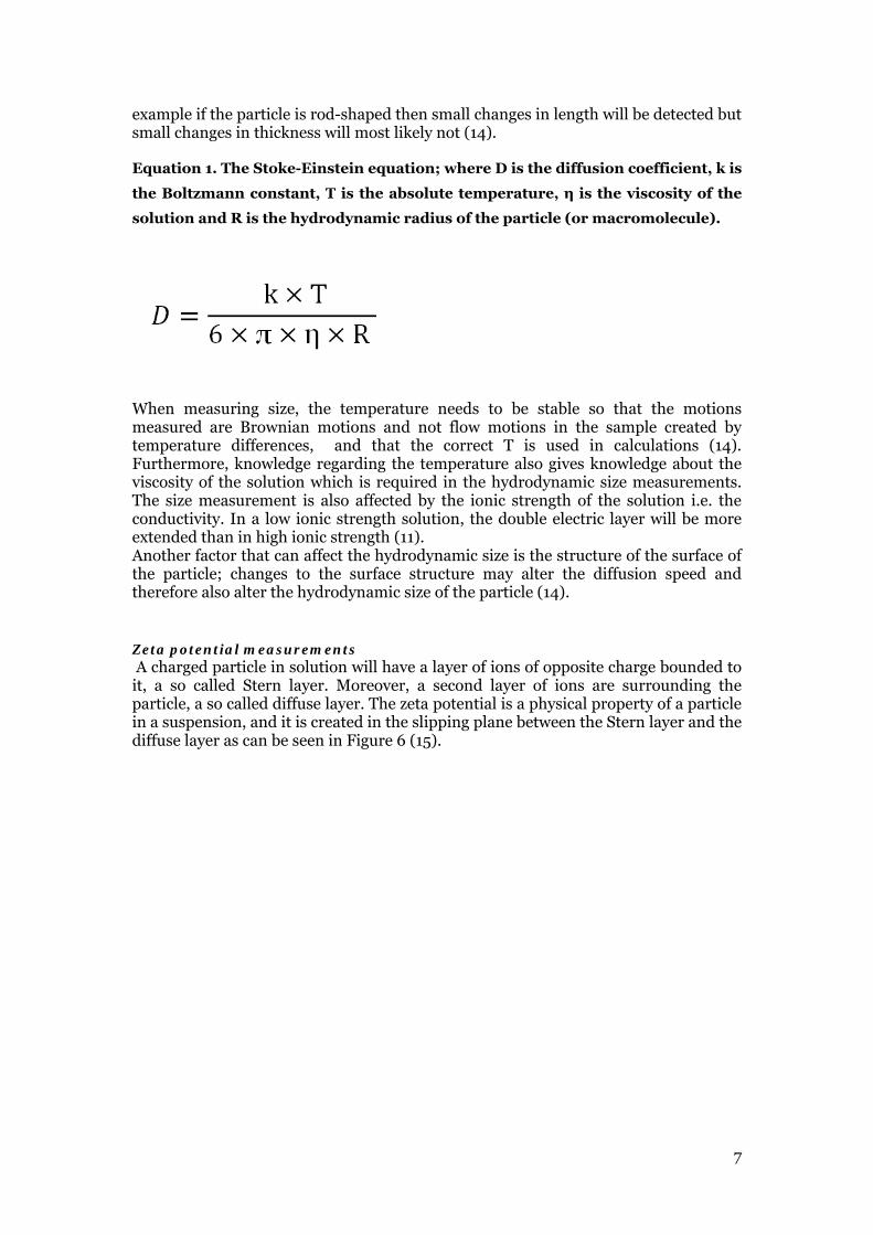
example if the particle is rod-shaped then small changes in length will be detected but small changes in thickness will most likely not (14). Equation 1. The Stoke-Einstein equation; where D is the diffusion coefficient, k is
the Boltzmann constant, T is the absolute temperature, η is the viscosity of the
solution and R is the hydrodynamic radius of the particle (or macromolecule).
When measuring size, the temperature needs to be stable so that the motions measured are Brownian motions and not flow motions in the sample created by temperature differences, and that the correct T is used in calculations (14). Furthermore, knowledge regarding the temperature also gives knowledge about the viscosity of the solution which is required in the hydrodynamic size measurements. The size measurement is also affected by the ionic strength of the solution i.e. the conductivity. In a low ionic strength solution, the double electric layer will be more extended than in high ionic strength (11). Another factor that can affect the hydrodynamic size is the structure of the surface of the particle; changes to the surface structure may alter the diffusion speed and therefore also alter the hydrodynamic size of the particle (14).
Zeta potential measurements A charged particle in solution will have a layer of ions of opposite charge bounded to it, a so called Stern layer. Moreover, a second layer of ions are surrounding the particle, a so called diffuse layer. The zeta potential is a physical property of a particle in a suspension, and it is created in the slipping plane between the Stern layer and the diffuse layer as can be seen in Figure 6 (15).

8
Figure 6. Schematic representation of zeta potential.
The zeta potential can indicate the degree of interaction between particles in a colloid system, and consequently the stability of the same system. A near neutral zeta value (-10 to 10 mV) or a zeta value of zero (isoelectric point) is an indication of an unstable system i.e. the particles will flocculate. In contrast to a strongly negative (lower than -30 mV) or strongly positive (higher than 30 mV) zeta potential that indicates a stable system i.e. the particles will repel each other and remain in solution (13), (15). It can also be used to investigate the surface charge of a particle since the zeta potential is dependent on the surface charge. However, the absolute zeta potential value will be lower than the surface charge, due to the ions in the double electrical layer (13), (15) (14). The zeta potential is measured by measuring the electrophoretic mobility of the particle. As the particle move the scattered light is phase shifted and this phase shift is proportional to the zeta potential of the particle. The data is correlated to zeta potential via the Henry equation as can be seen in Equation 2 (15).

9
Equation 2. Henrys equation (15).
Several different factors, such as the strength of the electric field, the dielectric constant (ε) of the medium, the viscosity (ŋ) of the medium and the zeta potential (Z) of the particle, affect the electrophoretic mobility (U(E)) (13), (15). The Henry function f (κa) is a function of the ratio between the radius of the particle and the thickness of the electrical double layer. For aqueous media with moderate electrolyte concentration this value will be 1.5 and these conditions are referred to as the Smoluchowski approximation (15). The zeta potential is affected by several factors such as pH and conductivity of the medium. For pH effects it can be seen that a particle in an alkaline solution generally will have a more negative zeta potential and a particle in an acid solution will have a more positive zeta potential (13). Furthermore, earlier in this report it was described that the hydrodynamic size was affected by ionic strength. The same can be said regarding the zeta potential although, in this case it is the interaction between the particle surface and surrounding ions that can change the zeta potential (15).
Method
Samples Table 2. Bacteria strains used in this study.
E.coli strain Modified gene BW25113 WT RN103 ΔwaaF RN104 ΔwaaG RN105 ΔwaaL RN106 ΔwaaP RN107 ΔgalE BW25113/pMF19 WT-o-antigen E.coli strain without flagella Modified gene BW25113 WT/flhD RN101 ΔwaaC RN102 ΔwaaE RN103 ΔwaaF/flhD RN104 ΔwaaG/fhlD RN105 ΔwaaL/flhD RN106 ΔwaaP/flhD RN107 ΔgalE/flhD Strains for vesicle production Modified gene BW25113 WT/flhD RN103 ΔwaaF/flhD RN104 ΔwaaG/fhlD RN105 ΔwaaL/flhD RN106 ΔwaaP/flhD RN107 ΔgalE/flhD
10
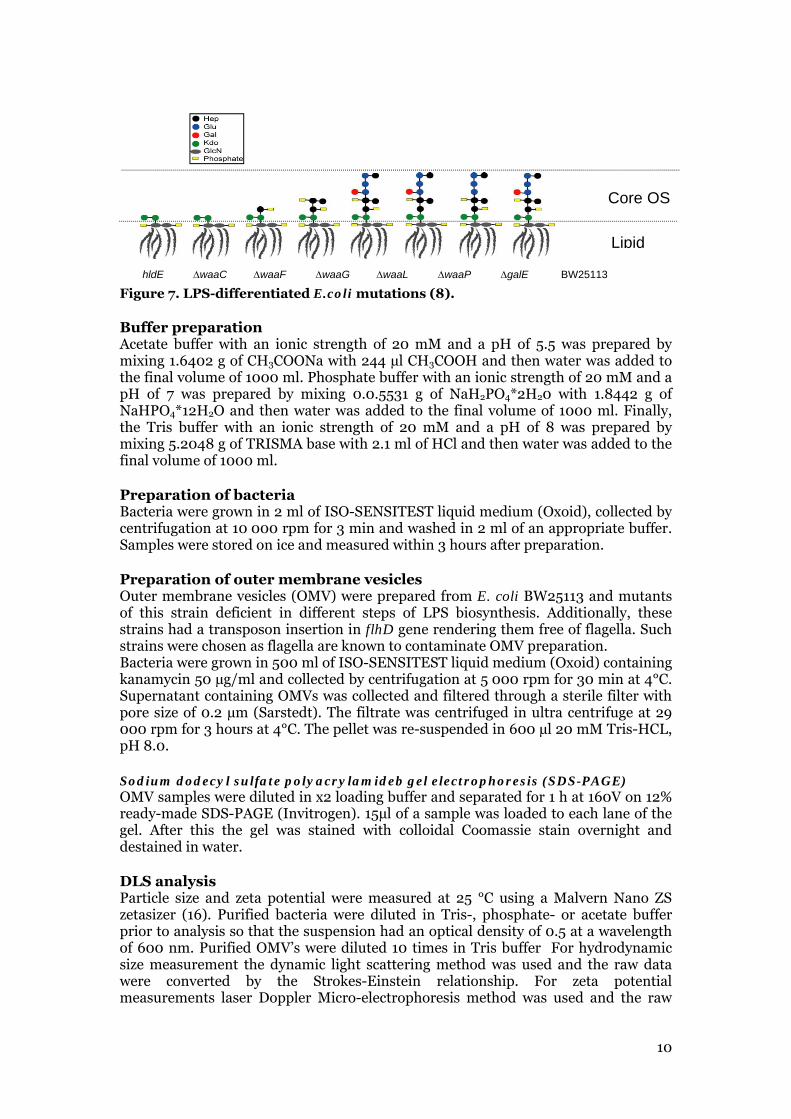
Figure 7. LPS-differentiated E.coli mutations (8).
Buffer preparation Acetate buffer with an ionic strength of 20 mM and a pH of 5.5 was prepared by mixing 1.6402 g of CH3COONa with 244 µl CH3COOH and then water was added to the final volume of 1000 ml. Phosphate buffer with an ionic strength of 20 mM and a pH of 7 was prepared by mixing 0.0.5531 g of NaH2PO4*2H20 with 1.8442 g of NaHPO4*12H2O and then water was added to the final volume of 1000 ml. Finally, the Tris buffer with an ionic strength of 20 mM and a pH of 8 was prepared by mixing 5.2048 g of TRISMA base with 2.1 ml of HCl and then water was added to the final volume of 1000 ml.
Preparation of bacteria Bacteria were grown in 2 ml of ISO-SENSITEST liquid medium (Oxoid), collected by centrifugation at 10 000 rpm for 3 min and washed in 2 ml of an appropriate buffer. Samples were stored on ice and measured within 3 hours after preparation.
Preparation of outer membrane vesicles Outer membrane vesicles (OMV) were prepared from E. coli BW25113 and mutants of this strain deficient in different steps of LPS biosynthesis. Additionally, these strains had a transposon insertion in flhD gene rendering them free of flagella. Such strains were chosen as flagella are known to contaminate OMV preparation. Bacteria were grown in 500 ml of ISO-SENSITEST liquid medium (Oxoid) containing kanamycin 50 µg/ml and collected by centrifugation at 5 000 rpm for 30 min at 4°C. Supernatant containing OMVs was collected and filtered through a sterile filter with pore size of 0.2 µm (Sarstedt). The filtrate was centrifuged in ultra centrifuge at 29 000 rpm for 3 hours at 4°C. The pellet was re-suspended in 600 µl 20 mM Tris-HCL, pH 8.0.
Sodium dodecyl sulfate polyacrylamideb gel electrophoresis (SDS-PAGE) OMV samples were diluted in x2 loading buffer and separated for 1 h at 160V on 12% ready-made SDS-PAGE (Invitrogen). 15µl of a sample was loaded to each lane of the gel. After this the gel was stained with colloidal Coomassie stain overnight and destained in water.
DLS analysis Particle size and zeta potential were measured at 25 °C using a Malvern Nano ZS zetasizer (16). Purified bacteria were diluted in Tris-, phosphate- or acetate buffer prior to analysis so that the suspension had an optical density of 0.5 at a wavelength of 600 nm. Purified OMV’s were diluted 10 times in Tris buffer For hydrodynamic size measurement the dynamic light scattering method was used and the raw data were converted by the Strokes-Einstein relationship. For zeta potential measurements laser Doppler Micro-electrophoresis method was used and the raw
hldE waaC waaF waaG waaL waaP galE BW25113
Core OS
Lipid

11
data were converted by the Smoluchowski approximation. For both size and zeta measurements a clear disposable zeta cell was used during analysis.
ATR-FTIR spectroscopic analysis The chemical composition was analyzed using a Bruker Vertex 80v spectrometer (17) with a 3 reflection ZnSe crystal plate placed on a MIRacle base optics assembly (18). Bacteria and OMV samples were centrifuged and the suspension removed. The pellet was then placed on the ATR crystal. For OMVs the samples had to be frozen with liquid nitrogen to enable transfer from the sample tube and placement on the crystal, this was due to the small amount of purified OMVs and also because of the slimy texture of the OMVs. Buffer spectra were also obtained and later subtracted from the other spectra.
Results and discussion
Optimization of the method The project started by developing an analysis method for bacteria as well as for vesicles. First of all, the lowest possible ionic strength of the buffer solution had to be established to ensure that the conductivity remained as low as possible but also to guarantee that the bacteria stay intact during the analysis. During some initial sample preparation there were indications of bacterial leakage for Pseudomonas aeruginosa at the ionic strength of 10 mM. The same leakage was not detected for E. coli indicating a more robust cell. Although to ensure that the most suitable ionic strength were used, tests with different ionic strength of phosphate buffer were performed. As can be seen in Figure 8, the zeta potential gets less negative the higher the ionic strength. This is due to that there are more ions in the solution that can screen the surface charge and therefore lowering the absolute zeta potential value. However, for ΔwaaC at ionic strength of 10 mM and 20 mM, it can be seen that the zeta potential is slightly higher at 20 mM indicating that there might be some instabilities in E.coli at 10 mM ionic strength. Analysis of viability did not show a large difference between 10 mM and 20 mM. However, for the rest of the measurements an ionic strength of 20 mM was used.
Figure 8. Variations in zeta potential, for ∆waaC and WT, due to alterations regarding the ionic strength of the phosphate buffer.
Growth conditions for the bacteria were also optimized; we compared properties of bacteria grown on blood agar plate or in liquid media. Both size and zeta potential values showed that the media did not have substantial influence on the results although standard deviation values were somewhat larger for the bacteria grown on
‐70
‐60
‐50
‐40
‐30
‐20
‐10
0
10 mM 20 mM 50 mM 100 mM
Zeta potential (mV)
Ionic strength
WaaC
WT

12
blood agar plate, as can be seen in Figure 9a and b, so the rest of the measurements were done with bacteria grown in liquid ISO-SENSITEST media.
a b Figure 9. Effects from growing sample on different culture media (blood plate or liquid media), on hydrodynamic size (a) and on zeta potential (b).
The vesicle production was a time-consuming process so to save time as well as sample the vesicles were stored in a freezer after DLS analysis and then used for IR after defrosting. To ensure that the vesicles stay stable during freezing, DLS analyses were preformed before and after freezing and the result can be seen in Figure 10a and b. There was some effect although it did not follow any trend and it was relatively small. The source of the difference could be from either the freezing process or the defrosting of the samples. The difference could also be due to uncertanties in the measuring method; giving a higher uncertanty of the absolut zeta potential value when the zeta potential was close to zero. Due to the small difference, the conclusion was made that the vesicle samples could be stored in the freezer.
a b Figure 10. Effects on hydrodynamic size (a) and zeta potential (b) from freezing vesicle sample.
Three different buffers were used with three different pH; one acid, one alkaline and one neutral solution. These buffers were used during analyses of bacteria to establish the most suitable buffer for analyses of bacteria and vesicles. As can been seen in Figure 11, bacteria in all buffers follow the same trend. Although bacteria in phosphate buffer tended to have the most negative zeta potential and bacteria in actetate buffer tended to have the least negative zeta potential. This result does not follow the expected trend were the most alkaline solution would have the most negative zeta potential, although, these differences seem to be mainly within the standard deviation. From these analyses only, it is difficult to make a conclusion on which buffer would be the most suitible for vesicle analysis as they only differ in zeta value within the same strain but follow the same trend between the strains. But we can make the conclusion that neither pH nor chemical composition of the buffer influence the zeta
0
1000
2000
3000
waaC‐LB waaC‐blood
Hydrodynam
ic size
(d.nm)
Bacterial strain‐65
‐63
‐61
‐59
‐57
‐55
waaC‐LB waaC‐blood
Zeta potential (mV)
Bacteria strain
0
50
100
150
200
250
300
350
ΔwaaF WT
Hydrodynam
ic size (d.nm)
Bacteria strain
Freshsample
Defrosted sample
‐10
‐8
‐6
‐4
‐2
0
ΔwaaF WT
Zeta potential (mV)
Bacteria strain
Freshsample
Defrosted sample

13
potential of bacteria to any greater extend. It does not change the correlation between two strains in the same kind of buffer. Figure 11 can also give an indication of how different alteration to the LPS chains will effect the zeta potential. As can be seen there are two groups of bacteria, those with long LPS chain (∆waaL, ∆waaP, ∆galE and WT) and those with short LPS chain (∆waaC, ∆waaE, ∆waaF and ∆waaG). From the result there can be seen that there is no indication of effects from flagella, mutants with and without flagella seem to have the same zeta potential. There can also be seen that the mutants with long LPS chain have a lower zeta potential and vice versa. And if comparing the mutants with long LPS chain with WT there is only small differences in zeta potential indicating that small changes to the LPS chain do not effect the zeta potential to any greater extend. For the WT with additional o-antigen, the LPS chain is even longer since the o-antigen is added to the LPS chain. Consequently, it will have a less negative zeta potential than WT as can be seen in Figure 11. Exacly how the different components in the LPS chain is affecting the zeta potential is not in the scope of this project, to establish that, further reseach will be needed. But from the data it can be concluded that larger changes in length of LPS influences the zeta potential.
Figure 11. Zeta potential for different bacteria strain, in three different buffers, each with different pH.
From the OPLS-DA multivariate Scores plot of ATR-FTIR spectroscopic data of the bacterial strains (Figure 12a, 13a and 14a) it can be seen that the higher the pH the more clear is the separation of the samples, based on the type of LPS mutations. Instead of Scores plot, the model overview an be used to gain more comprehensive information about the separation. A model overview shows if there is any significant difference between the different components and if so, how many components that exhibit a significant differences between them. The more components that can be differentiated from each other, the better is the separation of the difference substances. From this result, there can be seen that the most suitable buffer for analysing bacteria and vesicles would be Tris buffer, due to that seven different components could be identified in the multivarite analysis, as can be seen in Figure 12b, 13b and 14b. Bacteria in acetate buffer and phosphate buffer are less easily separable, most likely due to the bacterial surface is protonated or changed, in the buffers of lower pH which makes the different strains more similar to each other and/or more different within the biological replicates of a particlular strain. One reasonable explanation would be that the phosphates and amines on protein residues and the LPS chain get protonated and/or that the cells release something to the surface. Since the tris buffer seemed to best separate the different samples this buffer
‐70
‐60
‐50
‐40
‐30
‐20
‐10
0
Zeta potential (mV)
Bacteria strain
Acetate
Phosphate
Tris

14
was chosen for the remaining work. From now on in this report all samples shown were prepared and alaysed in Tris buffer.
a b
Figure 12. Scattered plot (a) and model overview (b) of bacteria in acetate buffer. Numbers of components = 1+1, Number of observations = 16, Number of classes = 6, R2X = 0,827, R2Y = 0,155, Q2 = -0,135.
c d
Figure 13.Scattered plot (a) and model overview (b) of bacteria in phosphate buffer. Numbers of components = 2+0, Number of observations = 16, Number of classes = 8, R2X = 0,759, R2Y = 0,218, Q2 = -0,0716.
e f
Figure 14. Scattered score plot (s) and model overview (b) of bacteria in Tris buffer. Numbers of components = 7 + 2, Number of observations = 16, Number of classes = 8, R2X = 0,993, R2Y = 0,899, Q2 = -0,276.
DLS analyses One hypothesis was that those E. coli mutants and their vesicles that have the shortest LPS chain would have a smaller hydrodynamic size. All sizes measured in this report are the hydrodynamic diameter of the particle and measured in nm. If Figure 15a and b is compared to Figure 7, it can be seen that the hydrodynamic size does not follow the expected trend for either vesicles or bacteria. For bacteria the
-25
-20
-15
-10
-5
0
5
10
15
20
25
-50 -40 -30 -20 -10 0 10 20 30 40 50
to[1
]
t[1]
WT____AB_0
WT____AB_1
WC____AB_0
WC____AB_1
WE____AB_0
WE____AB_1
WF____AB_0
WF____AB_1
WG____AB_0WG____AB_1
WL____AB_0
WL____AB_1
WP____AB_0
WP____AB_1
gE____AB_0
gE____AB_1
-0,1
0,0
0,1
0,2
0,3
0,4
0,5
0,6
0,7
0,8
0,9
Com
p[1]
P
SofiaC_Bacteria_2pointBaseline_new5.M24 (OPLS/O2PLS-DA) R2Y(cum)Q2(cum)
-20
-10
0
10
20
-40 -30 -20 -10 0 10 20 30 40
t[2]
t[1]
WT____PB_0
WT____PB_1
WC____PB_0WC____PB_1
WE____PB_0
WE____PB_1WF____PB_0
WF____PB_1
WG____PB_0
WG____PB_1
WL____PB_0
WL____PB_1WP____PB_0
WP____PB_1
gE____PB_0 gE____PB_1
-0,1
0,0
0,1
0,2
0,3
0,4
0,5
0,6
0,7
0,8
0,9C
om
p[1
]P
Co
mp[
2]P
SofiaC_Bacteria_2pointBaseline_new5.M25 (OPLS/O2PLS-DA) R2Y(cum)Q2(cum)
-25
-20
-15
-10
-5
0
5
10
15
20
25
-40 -35 -30 -25 -20 -15 -10 -5 0 5 10 15 20 25 30 35 40
t[2]
t[1]
WT____TB_0WT____TB_1
WC____TB_0
WC____TB_1WE____TB_0
WE____TB_1
WF____TB_0
WF____TB_1WG____TB_0
WG____TB_1
WL____TB_0
WL____TB_1
WP____TB_0
WP____TB_1
gE____TB_0
gE____TB_1
-0,1
0,0
0,1
0,2
0,3
0,4
0,5
0,6
0,7
0,8
0,9
Com
p[1]
P
Com
p[2]
P
Com
p[3]
P
Com
p[4]
P
Com
p[5]
P
Com
p[6]
P
Com
p[7]
P
Comp No.
SofiaC_Bacteria_2pointBaseline_new5.M23 (OPLS/O2PLS-DA) R2Y(cum)Q2(cum)
15
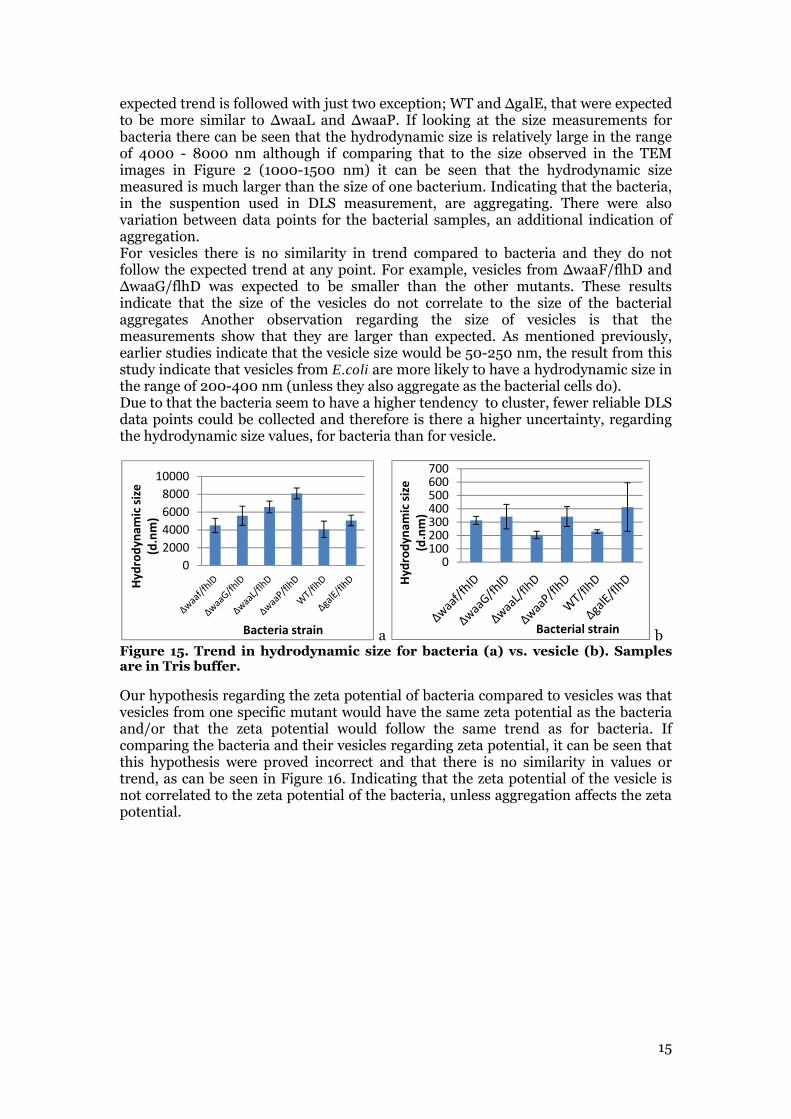
expected trend is followed with just two exception; WT and ∆galE, that were expected to be more similar to ∆waaL and ∆waaP. If looking at the size measurements for bacteria there can be seen that the hydrodynamic size is relatively large in the range of 4000 - 8000 nm although if comparing that to the size observed in the TEM images in Figure 2 (1000-1500 nm) it can be seen that the hydrodynamic size measured is much larger than the size of one bacterium. Indicating that the bacteria, in the suspention used in DLS measurement, are aggregating. There were also variation between data points for the bacterial samples, an additional indication of aggregation. For vesicles there is no similarity in trend compared to bacteria and they do not follow the expected trend at any point. For example, vesicles from ∆waaF/flhD and ∆waaG/flhD was expected to be smaller than the other mutants. These results indicate that the size of the vesicles do not correlate to the size of the bacterial aggregates Another observation regarding the size of vesicles is that the measurements show that they are larger than expected. As mentioned previously, earlier studies indicate that the vesicle size would be 50-250 nm, the result from this study indicate that vesicles from E.coli are more likely to have a hydrodynamic size in the range of 200-400 nm (unless they also aggregate as the bacterial cells do). Due to that the bacteria seem to have a higher tendency to cluster, fewer reliable DLS data points could be collected and therefore is there a higher uncertainty, regarding the hydrodynamic size values, for bacteria than for vesicle.
a b Figure 15. Trend in hydrodynamic size for bacteria (a) vs. vesicle (b). Samples are in Tris buffer.
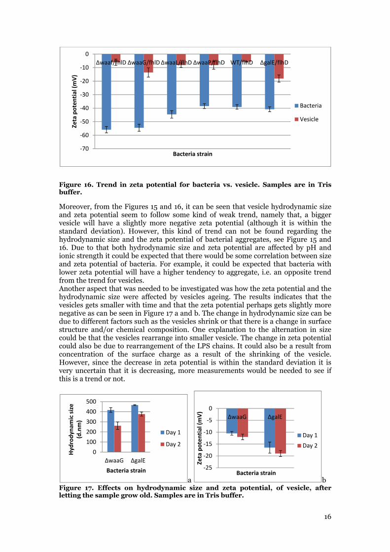
Our hypothesis regarding the zeta potential of bacteria compared to vesicles was that vesicles from one specific mutant would have the same zeta potential as the bacteria and/or that the zeta potential would follow the same trend as for bacteria. If comparing the bacteria and their vesicles regarding zeta potential, it can be seen that this hypothesis were proved incorrect and that there is no similarity in values or trend, as can be seen in Figure 16. Indicating that the zeta potential of the vesicle is not correlated to the zeta potential of the bacteria, unless aggregation affects the zeta potential.
0
2000
4000
6000
8000
10000
Hydrodynam
ic size
(d.nm)
Bacteria strain
0100200300400500600700
Hydrodynam
ic size
(d.nm)
Bacterial strain
16
Figure 16. Trend in zeta potential for bacteria vs. vesicle. Samples are in Tris buffer.
Moreover, from the Figures 15 and 16, it can be seen that vesicle hydrodynamic size and zeta potential seem to follow some kind of weak trend, namely that, a bigger vesicle will have a slightly more negative zeta potential (although it is within the standard deviation). However, this kind of trend can not be found regarding the hydrodynamic size and the zeta potential of bacterial aggregates, see Figure 15 and 16. Due to that both hydrodynamic size and zeta potential are affected by pH and ionic strength it could be expected that there would be some correlation between size and zeta potential of bacteria. For example, it could be expected that bacteria with lower zeta potential will have a higher tendency to aggregate, i.e. an opposite trend from the trend for vesicles. Another aspect that was needed to be investigated was how the zeta potential and the hydrodynamic size were affected by vesicles ageing. The results indicates that the vesicles gets smaller with time and that the zeta potential perhaps gets slightly more negative as can be seen in Figure 17 a and b. The change in hydrodynamic size can be due to different factors such as the vesicles shrink or that there is a change in surface structure and/or chemical composition. One explanation to the alternation in size could be that the vesicles rearrange into smaller vesicle. The change in zeta potential could also be due to rearrangement of the LPS chains. It could also be a result from concentration of the surface charge as a result of the shrinking of the vesicle. However, since the decrease in zeta potential is within the standard deviation it is very uncertain that it is decreasing, more measurements would be needed to see if this is a trend or not.
a b Figure 17. Effects on hydrodynamic size and zeta potential, of vesicle, after letting the sample grow old. Samples are in Tris buffer.
‐70
‐60
‐50
‐40
‐30
‐20
‐10
0
Δwaaf/fhlD ΔwaaG/fhlDΔwaaL/flhD ΔwaaP/flhD WT/flhD ΔgalE/flhD
Zeta potential (mV)
Bacteria strain
Bacteria
Vesicle
0
100
200
300
400
500
ΔwaaG ΔgalE
Hydrodynam
ic size
(d.nm)
Bacteria strain
Day 1
Day 2
‐25
‐20
‐15
‐10
‐5
0
ΔwaaG ΔgalE
Zeta potential (mV)
Bacteria strain
Day 1
Day 2
17
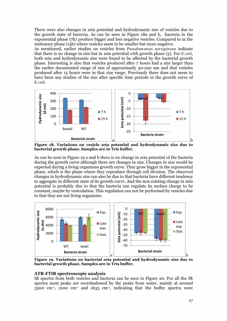
There were also changes in zeta potential and hydrodynamic size of vesicles due to the growth state of bacteria. As can be seen in Figure 18a and b, bacteria in the exponential phase (7h) produce bigger and less negative vesicles. Compared to in the stationary phase (15h) where vesicles seem to be smaller but more negative. As mentioned, earlier studies on vesicles from Pseudomonas aeruginosa indicate that there is no change in size but in zeta potential with growth phase (3). For E.coli, both zeta and hydrodynamic size were found to be affected by the bacterial growth phase. Interesting is also that vesicles produced after 7 hours had a size larger than the earlier documented range of size of approximatly 50-250 nm and that vesicles produced after 15 hours were in that size range. Previously there does not seem to have been any studies of the size after specific time periods in the growth curve of E.coli.
a b Figure 18. Variations on vesicle zeta potential and hydrodynamic size due to bacterial growth phase. Samples are in Tris buffer.
As can be seen in Figure 19 a and b there is no change in zeta potential of the bacteria during the growth curve although there are changes in size. Changes in size would be expected during a living organisms growth curve. They grow bigger in the exponential phase, which is the phase where they reproduce through cell division. The observed changes in hydrodynamic size can also be due to that bacteria have different tendency to aggregate in different state of its growth curve. And the non existing change in zeta potential is probably due to that the bacteria can regulate its surface charge to be constant, maybe by vesiculation. This regulation can not be performed by vesicles due to that they are not living organisms.
a b Figure 19. Variations on bacterial zeta potential and hydrodynamic size due to bacterial growth phase. Samples are in Tris buffer.
ATR-FTIR spectroscopic analysis IR spectra from both vesicles and bacteria can be seen in Figure 20. For all the IR spectra most peaks are overshadowed by the peaks from water, mainly at around 3300 cm-1, 2100 cm-1 and 1635 cm-1, indicating that the buffer spectra were
0
100
200
300
400
ΔwaaF WT
Hydrodynam
ic size
(d.nm)
Bacterial strain
7 h
15 h
‐25
‐20
‐15
‐10
‐5
0
ΔwaaF WT
Zeta potential (mV)
Bacteria strain
7 h
15 h
0
2000
4000
6000
8000
WT waaC
Hydrodynam
ic size
(n.dm)
Bacteria strain
Exp.
Lateexp.
Stat.
‐70
‐60
‐50
‐40
‐30
‐20
‐10
0
WT waaC
Zeta potential (mV)
Bacterial strain
Exp.
Lateexp.
Stat.

18
incompletely subtracted. Furthermore, there is also a region around 2900 cm-1 that corresponds to hydrocarbons mainly from lipids. Moreover, for E.coli bacteria, it can be seen a region between 1550 cm-1 and 1080 cm-1 that corresponds to vibrations from the proteins in the bacteria. Other components in this region will be overshadowed by the protein peaks, due to general abundance of proteins in bacteria. When comparing with the IR spectra of vesicles, the peaks corresponding to proteins are less intense or completely absent and there is another region in the area of 1100-800 cm-1, most likely corresponding to carbohydrates, that is more intense. This region of peaks is most likely present in bacteria spectra as well but due to the large amount of peptides the carbohydrate peaks will be relatively small. Another possible contribution to these peaks might be DNA or RNA although, due to the high amount of sugar in the vesicles, the DNA and RNA vibrations are most likely less pronounced. If looking even closer at the region between 1100 cm-1 and 1200 cm-1, in Figure 21, it can be seen that there are four main peaks; three of them differ from the spectra of bacteria. It is the peak at 1027, 1105 cm-1 and 1152 cm-1, the peak at 1082 cm-1 is represented in both vesicle spectra and bacteria spectra and most likely correspond to phosphate and sugar vibrations.
Figure 20. ATR-FTIR spectra for bacteria (red) and vesicles (black). Numbers indicates wavenumber (cm-1) of the peaks. Samples are in Tris buffer.
1546
1082
1027
1152
1105
2111
1456
1233
3287
1634
1397
100015002000250030003500
Wavenumber cm-1
0.0
0.2
0.4
0.6
0.8
Ab
sorb
an
ce U
nits

19
Figure 21. FTIR spectra of different vesicles compared to a ∆waaL bacterium spectra (light blue). The different vesicles spectra are as followed; ∆galE (pink), ∆waaF (black), ∆waaG (red), ∆waaL (blue), ∆waaP (green) och WT (grey). Numbers indicates wavelength (cm-1) of the peaks. Samples are in Tris buffer.
Comparisons of spectrum from IR analyses of bacteria and vesicles have been made using OPLS-DA multivariate analysis. The results are presented by Scores plots, Loadings plots and the original spectra. The three different presentations are all correlated. In the Loadings plot the areas at the positive side of the spectra will be more intensive in the samples on the positive side of the Scores plot and vice versa. Furthermore, there can also be seen which peaks in the original spectra that the peaks in the Loadings plot originates from. The P(corr) value in the Loadings plot is a value that indicates how much the samples differs at a specific wavenumber in the IR spectra. If the P(corr) value is strongly positive or negative then there is a strong difference between the samples. Conversely, if peak values in the Loadings plot are close to zero, there is a weak difference between the samples. Noteworthy, the data is total area normalized in OPUS; meaning that the intensity of the peaks is relative to each other and that changes in one area will alter the rest. This will have a consequence in the Loadings plot where big differences in small peaks will be overshadowed by small differences in large peak areas. Prior to the multivariate analysis, all spectra were baseline corrected and the buffer spectrum was subtracted from the other spectra. A comparison between bacteria and vesicle can be seen in Figures 22-25. The bacteria mutants are those without flagella due to that these are the ones that the vesicles originate from and it will also ensure that there is no influence from flagella on the results. In the Scores plot, Figure 22, a clear distinction between bacteria and vesicles can be seen. Comparing the Scores plot in Figure 22 to the Loadings plot in Figure 21, there can be seen that the peaks in the positive area of the Loadings plot corresponds to the samples marked black in the Scores plot, i.e. to the vesicle samples. Comparing the Loadings plot to the original spectra in Figure 24 and 25, there can be seen that the negative area, in the Loadings plot, correspond to the area marked black in the IR spectra. Comparing the Scores plot to the IR spectra, there can be seen that the area marked black in the IR spectra, is the peaks that differentiate vesicles from bacteria. The multivariate analysis result confirms the previous indications that the main component in the vesicle that differs from bacteria is the area of peaks in the region

20
around 1100-800 cm-1 (most likely from sugar) and the lack of peaks in the area of 1550 to 1080 cm-1 (most likely from proteins). From the differences in the positions in the Loadings plot for the peaks around 1637 cm-1 and 1549 cm-1 we can conclude that the water peak was not sufficiently subtracted. If it had been a peak at around 1637 cm-1 it would have represented a protein band and therefore followed the trend of the other protein bands.
Figure 22. PCA Scattering plot, bacteria (red) vs. vesicle (black). Samples are in Tris buffer. Numbers of components = 5, Number of observations = 18, Number of classes = 2, R2X = 0,912, Q2 = 0,763.
Figure 23. Loadings plot, bacteria (red) vs. vesicle (black). Numbers indicates wavelength (cm-1) of the peaks. Samples are in Tris buffer.
-30
-20
-10
0
10
20
30
-35 -30 -25 -20 -15 -10 -5 0 5 10 15 20 25 30 35
t[2]
t[1]
OPUS_Baseline_corrected_2pointbaseline_Areanorm2.M1 (PCA-X), Bacteria vs vesiclet[Comp. 1]/t[Comp. 2]Colored according to classes in M1
R2X[1] = 0,386934 R2X[2] = 0,287888 Ellipse: Hotelling T2 (0,95)
12
WF_fD_TB_b
WF_fD_TB_b
WG_fD_TB_bWG_fD_TB_bWL_fD_TB_bWL_fD_TB_b
WP_fD_TB_b
WP_fD_TB_b
WT_fD_TB_b
WT_fD_TB_b
gE_fD_TB_b
gE_fD_TB_b
WF_ve_TB_b
WG_ve_TB_b
WL_ve_TB_b
WP_ve_TB_b
WT_ve_TB_bgE_ve_TB_b
-1,0
-0,9
-0,8
-0,7
-0,6
-0,5
-0,4
-0,3
-0,2
-0,1
0,0
0,1
0,2
0,3
0,4
0,5
0,6
0,7
0,8
0,9
1,0
978
980
982
984
986
988
989
991
993
995
997
999
1001
1003
1005
1007
1009
1011
1013
1015
1016
1018
1020
1022
1024
1026
1028
1030
1032
1034
1036
1038
1040
1042
1043
1045
1047
1049
1051
1053
1055
1057
1059
1061
1063
1065
1067
1069
1070
1072
1074
1076
1078
1080
1082
1084
1086
1088
1090
1092
1094
1096
1097
1099
1101
1103
1105
1107
1109
1111
1113
1115
1117
1119
1121
1123
1124
1126
1128
1130
1132
1134
1136
1138
1140
1142
1144
1146
1148
1150
1151
1153
1155
1157
1159
1161
1163
1165
1167
1169
1171
1173
1175
1177
1178
1180
1182
1184
1186
1188
1190
1192
1194
1196
1198
1200
1202
1204
1205
1207
1209
1211
1213
1215
1217
1219
1221
1223
1225
1227
1229
1231
1232
1234
1236
1238
1240
1242
1244
1246
1248
1250
1252
1254
1256
1258
1259
1261
1263
1265
1267
1269
1271
1273
1275
1277
1279
1281
1283
1285
1286
1288
1290
1292
1294
1296
1298
1300
1302
1304
1306
1308
1310
1312
1313
1315
1317
1319
1321
1323
1325
1327
1329
1331
1333
1335
1337
1339
1340
1342
1344
1346
1348
1350
1352
1354
1356
1358
1360
1362
1364
1366
1367
1369
1371
1373
1375
1377
1379
1381
1383
1385
1387
1389
1391
1393
1394
1396
1398
1400
1402
1404
1406
1408
1410
1412
1414
1416
1418
1420
1421
1423
1425
1427
1429
1431
1433
1435
1437
1439
1441
1443
1445
1447
1448
1450
1452
1454
1456
1458
1460
1462
1464
1466
1468
1470
1472
1474
1475
1477
1479
1481
1483
1485
1487
1489
1491
1493
1495
1497
1499
1501
1502
1504
1506
1508
1510
1512
1514
1516
1518
1520
1522
1524
1526
1528
1529
1531
1533
1535
1537
1539
1541
1543
1545
1547
1549
1551
1553
1555
1556
1558
1560
1562
1564
1566
1568
1570
1572
1574
1576
1578
1580
1582
1583
1585
1587
1589
1591
1593
1595
1597
1599
1601
1603
1605
1607
1609
1610
1612
1614
1616
1618
1620
1622
1624
1626
1628
1630
1632
1634
1636
1637
1639
1641
1643
1645
1647
1649
1651
1653
1655
1657
1659
1661
1663
1664
1666
1668
1670
1672
1674
1676
1678
1680
1682
1684
1686
1688
1690
1691
1693
1695
1697
1699
1701
1703
1705
1707
1709
1711
1713
1715
1717
1718
1720
1722
1724
1726
1728
1730
1732
1734
1736
1738
1740
1742
1744
1745
1747
1749
1751
1753
1755
1757
1759
1761
1763
1765
1767
1769
1771
1772
1774
1776
1778
1780
1782
1784
1786
1788
1790
1792
1794
p(co
rr)[
1]
Var ID (Primary)
OPUS_Baseline_corrected_2pointbaseline_Areanorm3.M1 (PCA-X), Bacteria vs vesiclep(corr)[Comp. 1]
R2X[1] = 0,386934
1687
1610
1653
1477
1431
1362
1335
1187
1153
1105
1028
1005
982
1069
1088
1124
1173
1238
1313
1394
1454
1531
SIMCAP+12012012053114:05:22(UTC+1)

21
Figure 24. IR spectra for bacteria (red) and vesicle (black) correlated to the loadings plot. The numbers represent the wavelength (cm-1) of the peaks. Samples are in Tris buffer.
Figure 25. IR spectra for bacteria (red) and vesicle (black). The number represent wavelength (cm-1) of the peak. Samples are in Tris buffer.
Moreover, a comparison between the different vesicles can be seen in Figure 26-28. Due to lack of replicates when analyzing vesicles by IR spectroscopy, the analysis of the data will have a higher degree of uncertainty. In the Scores plot, Figure 26, there can be seen a clear distinction between ∆waaG, ∆waaP and ∆waaL. Moreover, WT, ∆waaF and ∆galE seem to be quite similar and the multivariate analysis is not able to distinguish between them. However, there is a clear difference between the group of WT, ∆waaF and ∆galE compared to the other three vesicle sample.
0,00
0,05
0,10
0,15
0,20
0,25
0,30
0,35
0,40
0,45
0,50
0,55
978
980
982
984
986
988
989
991
993
995
997
999
1001
1003
1005
1007
1009
1011
1013
1015
1016
1018
1020
1022
1024
1026
1028
1030
1032
1034
1036
1038
1040
1042
1043
1045
1047
1049
1051
1053
1055
1057
1059
1061
1063
1065
1067
1069
1070
1072
1074
1076
1078
1080
1082
1084
1086
1088
1090
1092
1094
1096
1097
1099
1101
1103
1105
1107
1109
1111
1113
1115
1117
1119
1121
1123
1124
1126
1128
1130
1132
1134
1136
1138
1140
1142
1144
1146
1148
1150
1151
1153
1155
1157
1159
1161
1163
1165
1167
1169
1171
1173
1175
1177
1178
1180
1182
1184
1186
1188
1190
1192
1194
1196
1198
1200
1202
1204
1205
1207
1209
1211
1213
1215
1217
1219
1221
1223
1225
1227
1229
1231
1232
1234
1236
1238
1240
1242
1244
1246
1248
1250
1252
1254
1256
1258
1259
1261
1263
1265
1267
1269
1271
1273
1275
1277
1279
1281
1283
1285
1286
1288
1290
1292
1294
1296
1298
1300
1302
1304
1306
1308
1310
1312
1313
1315
1317
1319
1321
1323
1325
1327
1329
1331
1333
1335
1337
1339
1340
1342
1344
1346
1348
1350
1352
1354
1356
1358
1360
1362
1364
1366
1367
1369
1371
1373
1375
1377
1379
1381
1383
1385
1387
1389
1391
1393
1394
1396
1398
1400
1402
1404
1406
1408
1410
1412
1414
1416
1418
1420
1421
1423
1425
1427
1429
1431
1433
1435
1437
1439
1441
1443
1445
1447
1448
1450
1452
1454
1456
1458
1460
1462
1464
1466
1468
1470
1472
1474
1475
1477
1479
1481
1483
1485
1487
1489
1491
1493
1495
1497
1499
1501
1502
1504
1506
1508
1510
1512
1514
1516
1518
1520
1522
1524
1526
1528
1529
1531
1533
1535
1537
1539
1541
1543
1545
1547
1549
1551
1553
1555
1556
1558
1560
1562
1564
1566
1568
1570
1572
1574
1576
1578
1580
1582
1583
1585
1587
1589
1591
1593
1595
1597
1599
1601
1603
1605
1607
1609
1610
1612
1614
1616
1618
1620
1622
1624
1626
1628
1630
1632
1634
1636
1637
1639
1641
1643
1645
1647
1649
1651
1653
1655
1657
1659
1661
1663
1664
1666
1668
1670
1672
1674
1676
1678
1680
1682
1684
1686
1688
1690
1691
1693
1695
1697
1699
1701
1703
1705
1707
1709
1711
1713
1715
1717
1718
1720
1722
1724
1726
1728
1730
1732
1734
1736
1738
1740
1742
1744
1745
1747
1749
1751
1753
1755
1757
1759
1761
1763
1765
1767
1769
1771
1772
1774
1776
1778
1780
1782
1784
1786
1788
1790
1792
1794
Var ID (Primary)
OPUS_Baseline_corrected_2pointbaseline_Areanorm3.DS1 OPUS_Baseline_corrected_2pointbaseline_AreanormObservation
1637
1549
1456 1394 1229
1153 1105
1078
1026
SIMCA-P+12.0.1-2012-05-3113:54:48(UTC+1)
-0,02
0,00
0,02
0,04
0,06
0,08
0,10
0,12
0,14
0,16
0,18
0,20
0,22
0,24
0,26
0,28
0,30
0,32
0,34
0,36
0,38
0,40
0,42
0,44
0,46
0,48
0,50
0,52
0,54
0,56
978
980
982
984
986
988
989
991
993
995
997
999
1001
1003
1005
1007
1009
1011
1013
1015
1016
1018
1020
1022
1024
1026
1028
1030
1032
1034
1036
1038
1040
1042
1043
1045
1047
1049
1051
1053
1055
1057
1059
1061
1063
1065
1067
1069
1070
1072
1074
1076
1078
1080
1082
1084
1086
1088
1090
1092
1094
1096
1097
1099
1101
1103
1105
1107
1109
1111
1113
1115
1117
1119
1121
1123
1124
1126
1128
1130
1132
1134
1136
1138
1140
1142
1144
1146
1148
1150
1151
1153
1155
1157
1159
1161
1163
1165
1167
1169
1171
1173
1175
1177
1178
1180
1182
1184
1186
1188
1190
1192
1194
1196
1198
1200
1202
1204
1205
1207
1209
1211
1213
1215
1217
1219
1221
1223
1225
1227
1229
1231
1232
1234
1236
1238
1240
1242
1244
1246
1248
1250
1252
1254
1256
1258
1259
1261
1263
1265
1267
1269
1271
1273
1275
1277
1279
1281
1283
1285
1286
1288
1290
1292
1294
1296
1298
1300
1302
1304
1306
1308
1310
1312
1313
1315
1317
1319
1321
1323
1325
1327
1329
1331
1333
1335
1337
1339
1340
1342
1344
1346
1348
1350
1352
1354
1356
1358
1360
1362
1364
1366
1367
1369
1371
1373
1375
1377
1379
1381
1383
1385
1387
1389
1391
1393
1394
1396
1398
1400
1402
1404
1406
1408
1410
1412
1414
1416
1418
1420
1421
1423
1425
1427
1429
1431
1433
1435
1437
1439
1441
1443
1445
1447
1448
1450
1452
1454
1456
1458
1460
1462
1464
1466
1468
1470
1472
1474
1475
1477
1479
1481
1483
1485
1487
1489
1491
1493
1495
1497
1499
1501
1502
1504
1506
1508
1510
1512
1514
1516
1518
1520
1522
1524
1526
1528
1529
1531
1533
1535
1537
1539
1541
1543
1545
1547
1549
1551
1553
1555
1556
1558
1560
1562
1564
1566
1568
1570
1572
1574
1576
1578
1580
1582
1583
1585
1587
1589
1591
1593
1595
1597
1599
1601
1603
1605
1607
1609
1610
1612
1614
1616
1618
1620
1622
1624
1626
1628
1630
1632
1634
1636
1637
1639
1641
1643
1645
1647
1649
1651
1653
1655
1657
1659
1661
1663
1664
1666
1668
1670
1672
1674
1676
1678
1680
1682
1684
1686
1688
1690
1691
1693
1695
1697
1699
1701
1703
1705
1707
1709
1711
1713
1715
1717
1718
1720
1722
1724
1726
1728
1730
1732
1734
1736
1738
1740
1742
1744
1745
1747
1749
1751
1753
1755
1757
1759
1761
1763
1765
1767
1769
1771
1772
1774
1776
1778
1780
1782
1784
1786
1788
1790
1792
1794
Var ID (Primary)
OPUS_Baseline_corrected_2pointbaseline_Areanorm3.DS1 OPUS_Baseline_corrected_2pointbaseline_AreanormObservation
1637
1549
1456 1394 1229
1153 1105
1078
1026

22
If the Scores plot in Figure 26 is correlated to the Loadings plot in Figure 27, it can be seen that the peaks in the negative area of the loadings plot corresponds to the vesicle samples in the negative area of the Scores plot, i.e. to WT, ∆waaF, ∆waaG and ∆galE. And in the same way do the peaks in the positive area of the Loadings plot correspond to the vesicle sample in the positive area of the Scores plot, i.e. to ∆waaL and ∆waaP. And if then looking at the Loadings plot and correlate it to the IR spectra in Figure 28, there can be seen that the negative area, in the Loadings plot, correspond to the area marked red in the IR spectra and vice versa for the area marked black. If we correlate the Scores plot to the IR spectra, it can be seen that the area marked black in the IR spectra, is the peaks where ∆waaL and ∆waaP differs from ∆waaF, ∆galE, ∆waaG and WT. This result indicates that vesicles from different mutants differ in chemical composition. And that the difference noticeable is most likely due to different sugar components, which also is logical since vesicles derivates from the outer membrane of bacteria with differences in sugar content, as can be seen in table 3.
Figure 26. The PCA Scores plot, vesicle comparison. Samples are in Tris buffer.The different vesicles spectra are as followed; ∆galE (pink), ∆waaF (black), ∆waaG (red), ∆waaL (blue), ∆waaP (green) och WT (orange). Numbers of components = 2, Number of observations = 6, Number of classes = 6, R2X = 0,798, Q2 = 0,343.
-50
-40
-30
-20
-10
0
10
20
30
40
50
-60 -50 -40 -30 -20 -10 0 10 20 30 40 50 60
t[2]
t[1]
OPUS_Baseline_corrected_2pointbaseline_Areanorm1.M2 (PCA-X), Vesicle comparisiont[Comp. 1]/t[Comp. 2]Colored according to classes in M2
R2X[1] = 0,427427 R2X[2] = 0,370143 Ellipse: Hotelling T2 (0,95)
123456
WF_ve_TB_b
WG_ve_TB_b
WL_ve_TB_b
WP_ve_TB_b
WT_ve_TB_bgE_ve_TB_b

23
Figure 27. Loadings plot, vesicle comparison. Black represents the vesicle on the positive side of the Scores plot and vice versa. Numbers indicates wavelength (cm-1) of the peaks in Tris buffer.
Figure 28. IR spectra correlated to the Loadings plot. Black represents the vesicle on the positive side of the Scores plot and vice versa. Numbers represent wavelength (cm-1) of the peaks. Samples are in Tris buffer.
Other data Some other data were provided for comparison from other scientist in the research group.
-1,0
-0,9
-0,8
-0,7
-0,6
-0,5
-0,4
-0,3
-0,2
-0,1
0,0
0,1
0,2
0,3
0,4
0,5
0,6
0,7
0,8
0,9
978
980
982
984
986
988
989
991
993
995
997
999
100
110
03
100
510
07
100
910
11
101
310
15
101
610
18
102
010
22
102
410
26
102
810
30
103
210
34
103
610
38
104
010
42
104
310
45
104
710
49
105
110
53
105
510
57
105
910
61
106
310
65
106
710
69
107
010
72
107
410
76
107
810
80
108
210
84
108
610
88
109
010
92
109
410
96
109
710
99
110
111
03
110
511
07
110
911
11
111
311
15
111
711
19
112
111
23
112
411
26
112
811
30
113
211
34
113
611
38
114
011
42
114
411
46
114
811
50
115
111
53
115
511
57
115
911
61
116
311
65
116
711
69
117
111
73
117
511
77
117
811
80
118
211
84
118
611
88
119
011
92
119
411
96
119
812
00
120
212
04
120
512
07
120
912
11
121
312
15
121
712
19
122
112
23
122
512
27
122
912
31
123
212
34
123
612
38
124
012
42
124
412
46
124
812
50
125
212
54
125
612
58
125
912
61
126
312
65
126
712
69
127
112
73
127
512
77
127
912
81
128
312
85
128
612
88
129
012
92
129
412
96
129
813
00
130
213
04
130
613
08
131
013
12
131
313
15
131
713
19
132
113
23
132
513
27
132
913
31
133
313
35
133
713
39
134
013
42
134
413
46
134
813
50
135
213
54
135
613
58
136
013
62
136
413
66
136
713
69
137
113
73
137
513
77
137
913
81
138
313
85
138
713
89
139
113
93
139
413
96
139
814
00
140
214
04
140
614
08
141
014
12
141
414
16
141
814
20
142
114
23
142
514
27
142
914
31
143
314
35
143
714
39
144
114
43
144
514
47
144
814
50
145
214
54
145
614
58
146
014
62
146
414
66
146
814
70
147
214
74
147
514
77
147
914
81
148
314
85
148
714
89
149
114
93
149
514
97
149
915
01
150
215
04
150
615
08
151
015
12
151
415
16
151
815
20
152
215
24
152
615
28
152
915
31
153
315
35
153
715
39
154
115
43
154
515
47
154
915
51
155
315
55
155
615
58
156
015
62
156
415
66
156
815
70
157
215
74
157
615
78
158
015
82
158
315
85
158
715
89
159
115
93
159
515
97
159
916
01
160
316
05
160
716
09
161
016
12
161
416
16
161
816
20
162
216
24
162
616
28
163
016
32
163
416
36
163
716
39
164
116
43
164
516
47
164
916
51
165
316
55
165
716
59
166
116
63
166
416
66
166
816
70
167
216
74
167
616
78
168
016
82
168
416
86
168
816
90
169
116
93
169
516
97
169
917
01
170
317
05
170
717
09
171
117
13
171
517
17
171
817
20
172
217
24
172
617
28
173
017
32
173
417
36
173
817
40
174
217
44
174
517
47
174
917
51
175
317
55
175
717
59
176
117
63
176
517
67
176
917
71
177
217
74
177
617
78
178
017
82
178
417
86
178
817
90
179
2
p(c
orr)
[1]
Var ID (Primary)
OPUS_Baseline_corrected_2pointbaseline_Areanorm3.M2 (PCA-X), Vesicle comparisionp(corr)[Comp. 1]
R2X[1] = 0 427427
1657
1792
1477
1566
1443
1126 1092
1067
1043
1009
1151
1327 1296 1259
11711192
0,00
0,05
0,10
0,15
0,20
0,25
0,30
0,35
0,40
0,45
0,50
0,55
978
980
982
984
986
988
989
991
993
995
997
999
1001
1003
1005
1007
1009
1011
1013
1015
1016
1018
1020
1022
1024
1026
1028
1030
1032
1034
1036
1038
1040
1042
1043
1045
1047
1049
1051
1053
1055
1057
1059
1061
1063
1065
1067
1069
1070
1072
1074
1076
1078
1080
1082
1084
1086
1088
1090
1092
1094
1096
1097
1099
1101
1103
1105
1107
1109
1111
1113
1115
1117
1119
1121
1123
1124
1126
1128
1130
1132
1134
1136
1138
1140
1142
1144
1146
1148
1150
1151
1153
1155
1157
1159
1161
1163
1165
1167
1169
1171
1173
1175
1177
1178
1180
1182
1184
1186
1188
1190
1192
1194
1196
1198
1200
1202
1204
1205
1207
1209
1211
1213
1215
1217
1219
1221
1223
1225
1227
1229
1231
1232
1234
1236
1238
1240
1242
1244
1246
1248
1250
1252
1254
1256
1258
1259
1261
1263
1265
1267
1269
1271
1273
1275
1277
1279
1281
1283
1285
1286
1288
1290
1292
1294
1296
1298
1300
1302
1304
1306
1308
1310
1312
1313
1315
1317
1319
1321
1323
1325
1327
1329
1331
1333
1335
1337
1339
1340
1342
1344
1346
1348
1350
1352
1354
1356
1358
1360
1362
1364
1366
1367
1369
1371
1373
1375
1377
1379
1381
1383
1385
1387
1389
1391
1393
1394
1396
1398
1400
1402
1404
1406
1408
1410
1412
1414
1416
1418
1420
1421
1423
1425
1427
1429
1431
1433
1435
1437
1439
1441
1443
1445
1447
1448
1450
1452
1454
1456
1458
1460
1462
1464
1466
1468
1470
1472
1474
1475
1477
1479
1481
1483
1485
1487
1489
1491
1493
1495
1497
1499
1501
1502
1504
1506
1508
1510
1512
1514
1516
1518
1520
1522
1524
1526
1528
1529
1531
1533
1535
1537
1539
1541
1543
1545
1547
1549
1551
1553
1555
1556
1558
1560
1562
1564
1566
1568
1570
1572
1574
1576
1578
1580
1582
1583
1585
1587
1589
1591
1593
1595
1597
1599
1601
1603
1605
1607
1609
1610
1612
1614
1616
1618
1620
1622
1624
1626
1628
1630
1632
1634
1636
1637
1639
1641
1643
1645
1647
1649
1651
1653
1655
1657
1659
1661
1663
1664
1666
1668
1670
1672
1674
1676
1678
1680
1682
1684
1686
1688
1690
1691
1693
1695
1697
1699
1701
1703
1705
1707
1709
1711
1713
1715
1717
1718
1720
1722
1724
1726
1728
1730
1732
1734
1736
1738
1740
1742
1744
1745
1747
1749
1751
1753
1755
1757
1759
1761
1763
1765
1767
1769
1771
1772
1774
1776
1778
1780
1782
1784
1786
1788
1790
1792
1794
Var ID (Primary)
OPUS_Baseline_corrected_2pointbaseline_Areanorm3.DS1 OPUS_Baseline_corrected_2pointbaseline_AreanormObservation
WF_ve_TB_br1_2404_BC_0WG_ve_TB_br1_1505_BC_0WL_ve_TB_br1_0705_BC_0WP_ve_TB_br1_1105_BC_0WT_ve_TB_br1_1005_BC_0gE_ve_TB_br1_1105_BC_0
1026
1078
1103
1153
1639
SIMCAP+12012012053114:28:37(UTC+1)

24
SDS-PAGE A SDS-PAGE gel of vesicles from different bacteria mutants, see Figure 29, showed the most protein content in ΔwaaG (mainly at 45 kD, 30 kD and 20 kD), followed by ΔwaaF, ΔwaaP and galE (at 45 kD and 30 kD). There seem to be some proteins in ΔwaaL (at 45 kD) as well, although for WT the bands are too weak to tell if anything is there. The lack of bands in the gel for WT indicates that those vesicles have a lesser amount of proteins. What kind of proteins the different mutants release with their vesicles is still unknown although, there is no indication that they are solution proteins from cell leakage. If the proteins would have been from cell leakage there would have been a high amount of bands all over the gel. Moreover, it seems like most mutants have the same proteins i.e. the bands in the gel are at the same position, an indication of similar molecular weight. If this protein content is compared with the size of vesicles as can be seen in Figures 10 and 15b, there could be some indication of a correlation due to that the vesicles with the lowest amounts of proteins also are the once with the smallest hydrodynamic size. However, the data points are too few to make any clear conclusions or to make any correlations to the DLS or the IR spectroscopic data.
Figure 29. SDS-Page of E.coli vesicles.
X-ray photoelectron spectroscopy, XPS If looking at the XPS data for the different bacteria mutants there can be seen that most bacteria have a high content of peptides and less of sugar and lipids. With one exception for ΔwaaE, were the lipid content is slightly higher than the peptide content. Why is unknown, however a possible explanation could be that the length and composition of the LPS chain is affecting the protein content. Furthermore, if comparing the vesicle sample with the bacterium sample of the same mutant, ∆waaL, there can be seen that the vesicle have a higher contents of lipids than bacterium and a low contents of both peptides and sugar. These data support the data extracted from the IR spectroscopic analyses regarding the low peptide contents in vesicles and the visible variation in sugar contents of vesicles.
LadderWTΔwaaLΔwaaPΔgalEΔwaaGΔwaaF
k
105 84 50 36 28
12% SDS‐PAGE of E.coli

25
Table 3. Multianalysis of C 1s XPS spectra, table shows the % contents of total carbon in the sample,
Sample Peptide Lipid Sugar WT 53 27 20 ΔwaaC 58 32 10 ΔwaaE 39 49 12 ΔwaaF 69 19 13 ΔwaaG 67 18 15 ΔwaaP 74 10 16 ΔgalE 69 11 20 ΔwaaL 75 7 18 ΔwaaL/fhlD 62 18 20 ves ΔwaaL 18 63 19
26
Conclusions
For the DLS data there could be seen some very interesting trends regarding the factors affecting vesicles and the production of them. First of all, the results indicate that the composition of the LPS chain of bacteria is an important factor affecting the zeta potential. Furthermore, this study also indicates that there is no direct correlation between bacterial zeta potential and the vesicle zeta potential. However, there is indication that the growth phase of the bacteria is a factor that affects both the zeta potential and the hydrodynamic size of vesicles. Making them smaller and more negative the later in the growth they are collected. Vesicles are also affected by ageing, getting smaller and slightly more negative by time. However, since there is an uncertainty regarding the aggregation of the sample during DLS analyses all conclusions have a high degree of uncertainty and should be treated thereafter. Further analyses are needed to verify the results in this study. From the IR spectroscopic results a clear difference between vesicles and bacteria could be seen indicating a difference in chemical composition. However, the IR spectroscopic analyses have a higher degree of uncertainty than the DLS data due to a smaller amount of data points. Moreover, even though the intentions were to subtract the buffer, the results indicate an incomplete subtraction. So to gain more information regarding the components a complete subtraction is needed in the future. Analyzing the spectra in combination with XPS data, the differences is suggested to be from different amount of peptides and lipids, where a lower peptide contents in vesicle reveals the sugar peaks in the spectra. The main component in vesicle seems to be lipids although those peaks are still mostly overshadowed by peaks corresponding to water. Sugar peaks seem to differ indicating that the sugar components varies among the vesicles. What kind of differences there are and how big the differences are, is still unknown and further research is needed. To sum up, there does not seem to be any direct correlation between the zeta potential of vesicles and bacteria indicating that vesicles cannot be used as a model for the bacterial surface. However, there are interesting trends emerging from these results, which need to be further investigated. There are also a lot of questions arising from this pilot study. For example, what exactly does happen to vesicles after they are released? What are the factors that control the contents of the vesicles? If the surface characteristics are independent from the bacteria they originate from, what other factors affect the surface? These questions and more will hopefully be answered in future research.
Acknowledgement
A huge thank to my supervisor Madeleine Ramstedt for the help and support during the project. Always positive and encouraging, making it really nice working with you. Bringing out the best of each and everyone. You also manage something no one else has, to make me interested in research. Maybe I come back some day to find out why these “lovely” vesicles are acting like they do. And Olena Rzhepishevska (the red haired whirlwind/yrväder), what would I have done without you? Probably nothing, no samples – no work… András Gorzsás, thanks for making me understand multivariate analysis and for helping me when the IR spectrometer misbehaved. Peter Kallioniemi, you know I couldn’t have done this without you. Thanks for helping me understand the world of the living organisms and the world of English grammar.

27

28
Bibliography
1. N. Mozes, P. S. Handley, H. J. Busscher, P. G. Rouxhet. Microbial cell surface analysis. s.l. :
VCH Publishers, 2001.
2. Bacterial outer membrane vesicles and the host‐pathogen interaction. Meta J. Kuhen,
Nicole C. Kesty. s.l. : Cold Spring Harbour Laboratory Press, 2005, Genes & Development,
Vol. 19, pp. 2645‐2655.
3. Gram‐negative outer membrane vesicles: beyond the cell surface. L. Mashburn‐Warren, R.
J. C. McLean, M. Whiteley. Austin : Blacjwell Publishing Ltd, 2008, Geobiology, Vol. 6, pp.
214‐219.
4. Release of outer membrane vesicles by Gram‐negative bacteria is a novel envelope stress
respons. Amanda J. McBroom, Meta J. Kuhen. 2, s.l. : Blackwell Publishing Ltd, 2007,
Molecular Microbiology, Vol. 63, pp. 545‐558.
5. Virulence and immunomodulatory roles of bacterial outer membrane vesicles. Terri N.
Ellis, Meta J. Kuhen. 1, s.l. : American Society for Microbiology, 2010, Microbiology and
Molecular Biology Reviews, Vol. 74, pp. 81‐94.
6. Pineda, T. L. Bacterial species spectroscopic characterization by FTIR, normal RAMAN and
surface enhanced RAMAN scatterinmg. Chemistry. s.l. : University of Puerto Rico, 2006. Final
thesis .
7. Variation of physiochemical properties and cell association activity of membrane vesicles
with growth phase in Pseudomonas aeruginosa. Y. Tashiro, S. Ichikawa, M.Shimizu, M.
Toyofuku, N. Takaya, T.Nakajima‐Kambe, H. Uchiyama, N. Nomura. 11, s.l. : American
Society for Microbiology, June 2010, Applied and Environmental Microbiology , Vol. 76, pp.
3732‐3739.
8. Ramstedt, Madeleine. Personal communication . 2012.
9. Effect of surface lipopolysaccaride on the nature of membrane vesicles liberated from the
Gram‐negative bacterium Psedomonas aeruginosa. Trang T. Nguyen, Anu Saxena, Terry J.
Beveridge. 5, s.l. : Japanese Society of Microscopy, 2003, Journal of Electron Microscope,
Vol. 52, pp. 465‐469.
10. Characterization of the cell surface and cell wall chemistry of drinking water bacteria by
combining XPS, FTIR, modeling and potentiometric titrations. J. J. Ojeda, M. E. Romeo‐
González, R. T. Bachmann, R. G.J. Edyvean, S. A. Banwart. s.l. : American Chemical Society,
2008, Langmuir, Vol. 24, pp. 4032‐4040.
11. Stuart, Barbara. Infrared spectroscopy: fundamentals and applications. s.l. : Wiley, 2004.
12. Lambert, Joseph B. Vibrational spectroscopy. Organic structural spectroscopy. 2007, 7.
13. Zeta potential measurment. Jefferey D. Clogston, Anil K. Patri. Part 2, s.l. : Springer
Science , 2011, Methods in Molecular Biology, Vol. 697, pp. 63‐70.

29
14. Malvern. Dynamic light scattering: An introduction in 30 minutes. www.malvern.com.
[Online] 2012. [Cited: June 3, 2012.]
15. —. Zeta potential; an introduction in 30 minutes. www.malvern.com. [Online] 2012.
[Cited: June 3, 21012.]
16. www.malvern.com. Malvern . [Online] Malvern Instruments Ltd, 2012.
17. www.brukeroptics.com. Bruker optics. [Online] Bruker optics, 2012. [Cited: June 3, 2012.]
http://www.brukeroptics.com/vertex80.html?&print=1%EF%BF%3FL%3D10.
18. www.piketech.com. Pike Tech. [Online] Pike Technologies, 2012. [Cited: June 3, 2012.]
http://www.piketech.com/MIRacle‐TM‐Single‐Reflection‐ATR.html.
19. www.malvern.com. Malvern. [Online] Malvern Instruments Ltd, 2012. [Cited: June 3,
2012.]
www.malvern.com/labeng/products/zetasizer/zetasizer_nano/zetasizer_nano_zs.htm.

Department of Chemistry S-901 87 Umeå, Sweden Telephone +46 90 786 50 00 Text telephone +46 90 786 59 00 www.umu.se