
Supporting Online Material for -...
132
www.sciencemag.org/cgi/content/full/335/6076/1590/DC1 Supporting Online Material for Adapting to Osmotic Stress and the Process of Science Brittany J. Gasper, Dennis J. Minchella, Gabriela C. Weaver, Laszlo N. Csonka, Stephanie M. Gardner* *To whom correspondence should be addressed. E-mail: [email protected] Published 30 March 2012, Science 335, 1590 (2012) DOI: 10.1126/science.1215582 This PDF file includes Materials and Methods References
Transcript of Supporting Online Material for -...
www.sciencemag.org/cgi/content/full/335/6076/1590/DC1
Supporting Online Material for
Adapting to Osmotic Stress and the Process of Science
Brittany J. Gasper, Dennis J. Minchella, Gabriela C. Weaver, Laszlo N. Csonka, Stephanie M. Gardner*
*To whom correspondence should be addressed. E-mail: [email protected]
Published 30 March 2012, Science 335, 1590 (2012) DOI: 10.1126/science.1215582
This PDF file includes
Materials and Methods References

Genetic Analysis of Adaptation to Osmotic Stress in Salmonella -Weekly Summary
Week Lab Exercise Objectives
1 Illustration of the physical process of osmosis,
designing experiments, and introduction to aseptic
technique
I. Employ the scientific method to perform an experiment aimed at visualizing the physical process of osmosis
II. Utilize aseptic technique in the transferring of solutions using a micropipettor
2 Quantitative data analysis
methods, independent dilutions, preparation of solid bacterial growth media, and methods of
plating bacteria
I. Use descriptive and test statistics to interpret previous week’s data
II. Aseptically plate bacteria for isolated colonies using the quadrant streak and spread plate technique and prepare bacterial media using dilution calculations
3 Importance of mutants in
scientific research, auxotrophy the Salmonella typhimurium osmotic stress
response, and light microscopy
I. Perform an experiment to visualize the concept of auxotrophy and bacterial osmotic stress response (specifically understanding the role of ProP)
II. Use a compound light microscope to view osmotically stressed red blood cells
4 Use of spectrophotometry to
measure bacterial growth rates, streaking to a pure culture, and mutagenesis
I. Use a spectrophotometer to measure the absorbance of a solution and bacterial growth
II. Describe types of mutagenesis and understand the role mutations have on proteins and cell function
5 Quantification of substances
in solution with spectrophotometry and
mutagenesis
I. Perform serial dilutions, calculate dilution factors, determine the concentration of an unknown solution after generating a standard curve, and analyze a bacterial growth curve based on previous week’s data
II. Perform mutagenesis aimed at generation of proP mutants
6 Pinwheel streaking
technique, mutational frequency estimations,
inoculation of liquid media, and the theory of
transduction
I. Pinwheel streak mutants generated from the mutagenesis of the previous week
II. Estimate the mutation frequency of the different mutagenic techniques performed the previous week

7 Genetic Mapping, linkage, transduction, and Gram
staining
I. Perform a generalized transduction, selecting for antibiotic resistance, to begin determination of which mutants contain proP mutations
II. Perform a Gram stain to visually identify Gram positive and Gram negative bacteria
8 Screening transductants for
successful transduction of proP gene and growth in
original mutagenesis conditions
I. Pinwheel streak transductants onto the appropriate selective media to screen for mutants in proP
II. Understand the usage of gene linkage and antibiotic resistance in mapping the location of genetic mutations
9 Functional testing of
mutants and presenting data in poster format
I. Design and perform experiments to functionally characterize mutant phenotype of successful proP mutants (based on previous week’s data) and use a spectrophotometer to measure growth rate of proP mutants
II. Sketch an outline of research poster
10 Preparation for PCR amplification of the proP
gene
I. Prepare for PCR amplification and gel electrophoresis by reviewing the process and practicing loading solutions into gel wells
II. Organize, prepare, and present preliminary data to the class in the format of a 10 minute PowerPoint presentation
11 PCR amplification of the
proP gene and practicing sequencing proP gene
I. PCR amplify the proP gene from proP mutants II. Prepare and run an agarose gel to visualize successful
amplification of the proP gene
12 Sequencing and implication of point mutations in proP
I. Analyze and align mutant proP sequences with the wildtype proP sequence to identify the mutation location in the DNA sequence and translate into amino acids to identify the amino acid mutation
II. Model the membrane topology of ProP with play-doh and formulate hypotheses to explain the phenotype of the mutations based on the changes in its genotype
13-15 Poster preparation and
presentation I. Prepare and practice presenting poster II. Present poster in formal poster session attended by
department faculty, staff, and students

References and Notes
1. D. B. Luckie, J. J. Maleszewski, S. D. Loznak, M. Krha, Adv. Physiol. Educ. 28, 199 (2004).
2. G. C. Weaver, C. B. Russell, D. J. Wink, Nat. Chem. Biol. 4, 577 (2008).
3. AAAS, Vision and Change in Undergraduate Biology Education: A Call to Action (AAAS, Washington, DC, 2011).
4. C. A. Lindgren, Chronicle of Higher Education, 18 April 2010; http://chronicle.com/article/Teaching-Matters-Turning/65132/.
5. V. J. Dunlap, L. N. Csonka, J. Bacteriol. 163, 296 (1985).
6. G. C. Weaver et al., Chem. Educator 11, 125 (2006).
7. L. N. Csonka, A. D. Hanson, Annu. Rev. Microbiol. 45, 569 (1991).
8. D. E. Culham et al., Biochemistry 47, 13584 (2008).
9. B. J. Gasper et al., DNA Cell Biol., 10.1089/dna.2011.1510 (2012).
10. B. J. Gasper et al., J. Microbiol. Biol. Educ. 12(1), ASM Conference for Undergraduate Educators, abstr. 19-A (2011).
11. S. M. Gardner, O. A. Adedokun, G. C. Weaver, E. L. Bartlett, J. Undergrad. Neurosci. Educ. 10, A24 (2011).

BACTERIAL ADAPTATIONS TO OSMOTIC STRESS
A Project Created by
Dr. Stephanie Gardner, Dr. Brittany Gasper, and Dr. Laszlo Csonka
Department of Biological Sciences
Purdue University, West Lafayette, IN 47907
A CASPiE Project Module
CASPiE Module Bacterial Adaptations to Osmotic Stress
2
Table of contents
I. Introduction……………………………………………………………………………...4
1. Cells and plasma membranes and osmoregulation…………………………………...4
2. Bacteria as model organisms in the study of osmoregulation………………………..6
3. Summary of what isn’t known……………………………………………………….8
4. Module Calendar…………………………………………………………………......9
5. What is the Big Picture?.............................................................................................10
II. Laboratory Period 1…………………………………………………………………….11
1. Introduction………………………………………………………………………....11
2. Pre-laboratory activities……………………………………………………………..15
3. Materials…………………………………………………………………………….16
4. Procedures…………………………………………………………………………..17
5. Post-laboratory analysis and results…………………………………………………19
6. Preparation for the Next Laboratory Activity…………………………………….....19
III. Laboratory Period 2………………………………………………………………….....20
1. Introduction………………………………………………………………………....20
2. Pre-laboratory activities……………………………………………………………..30
3. Materials…………………………………………………………………………….30
4. Procedures…………………………………………………………………………...32
5. Post-laboratory analysis and results…………………………………………………34
6. Preparation for the Next Laboratory Activity…………………………………….....34
IV. Laboratory Period 3………………………………………………………………….....35
1. Introduction……………………………………………………………………….....35
2. Pre-laboratory activities……………………………………………………………..45
3. Materials…………………………………………………………………………….45
4. Procedures…………………………………………………………………………..47
5. Post-laboratory analysis and results…………………………………………………52
6. Preparation for the Next Laboratory Activity…………………………………….....52
V. Laboratory Period 4…………………………………………………………………….53
1. Introduction……………………………………………………………………….....53
2. Pre-laboratory activities……………………………………………………………..58
3. Materials…………………………………………………………………………….59
4. Procedures…………………………………………………………………………..60
5. Post-laboratory analysis and results…………………………………………………61
6. Preparation for the Next Laboratory Activity……………………………………....61
VI. Laboratory Period 5………………………………………………………………….....62
1. Introduction……………………………………………………………………….....62
2. Pre-laboratory activities……………………………………………………………..67
3. Materials…………………………………………………………………………….67
4. Procedures…………………………………………………………………………..68
5. Post-laboratory analysis and results…………………………………………………70
6. Preparation for the Next Laboratory Activity……………………………………....70
VII. Laboratory Period 6…………………………………………………………………….71
1. Introduction………………………………………………………………………....71
2. Pre-laboratory activities……………………………………………………………..76
3. Materials…………………………………………………………………………….76
4. Procedures…………………………………………………………………………..77

CASPiE Module Bacterial Adaptations to Osmotic Stress
3
5. Post-laboratory analysis and results…………………………………………………78
6. Preparation for the Next Laboratory Activity……………………………………....78
VIII. Laboratory Period 7………………………………………………………………….....79
1. Introduction………………………………………………………………………....79
2. Pre-laboratory activities…………………………………………………………….84
3. Materials…………………………………………………………………………….85
4. Procedures…………………………………………………………………………..86
5. Post-laboratory analysis and results…………………………………………………87
6. Preparation for the Next Laboratory Activity……………………………………....87
IX. Laboratory Period 8………………………………………………………………….....88
1. Introduction………………………………………………………………………....88
2. Pre-laboratory activities……………………………………………………………..89
3. Materials…………………………………………………………………………….89
4. Procedures…………………………………………………………………………..90
5. Post-laboratory analysis and results…………………………………………………91
6. Preparation for the Next Laboratory Activity……………………………………....91
X. Laboratory Period 9…………………………………………………………………….92
1. Introduction………………………………………………………………………....92
2. Pre-laboratory activities……………………………………………………………..96
3. Materials…………………………………………………………………………….96
4. Procedures…………………………………………………………………………..97
5. Post-laboratory analysis and results…………………………………………………98
6. Preparation for the Next Laboratory Activity……………………………………....98
XI. Laboratory Period 10…………………………………………………………………...99
1. Introduction………………………………………………………………………....99
2. Pre-laboratory activities……………………………………………………………103
3. Materials…………………………………………………………………………...104
4. Procedures………………………………………………………………………....104
5. Post-laboratory analysis and results……………………………………………….104
6. Preparation for the Next Laboratory Activity……………………………………..104
XII. Laboratory Period 11………………………………………………………………….105
1. Introduction………………………………………………………………………..105
2. Pre-laboratory activities…………………………………………………………....109
3. Materials…………………………………………………………………………...109
4. Procedures…………………………………………………………………………110
5. Post-laboratory analysis and results……………………………………………….111
6. Preparation for the Next Laboratory Activity…………………………………….. 111
XIII. Laboratory Period 12………………………………………………………………….112
1. Introduction………………………………………………………………………...112
2. Pre-laboratory activities……………………………………………………………118
3. Materials…………………………………………………………………………...118
4. Procedures………………………………………………………………………….119
5. Post-laboratory analysis and results………………………………………………..119
6. Preparation for the Next Laboratory Activity……………………………………...119
Appendix A – Bacterial Genetics Strain List………………………………………………….120
Appendix B - Bacterial Genetics Implementation Material…………………………………...121
Appendix C – Reference list and image information…………………………………………127
CASPiE Module Bacterial Adaptations to Osmotic Stress
4
I. Introduction
1. Cells and plasma membranes
The semipermeable plasma membrane
Cells, whether they are unicellular organisms or are part of a multicellular organism, are bound by a membrane
that separates the inside of the cell from its surroundings. The membrane is called ‘semi-permeable’ because it
allows cells to be selective about what they will allow to enter or leave them. The plasma membrane is made of
a phospholipid bilayer that has associated with it proteins and carbohydrates. The lipid portion of the
membrane acts as a barrier to most molecules, including inorganic ions, amino acids, and sugars. Many of these
substances can cross the plasma membrane, but do so through proteins that traverse the membrane known as
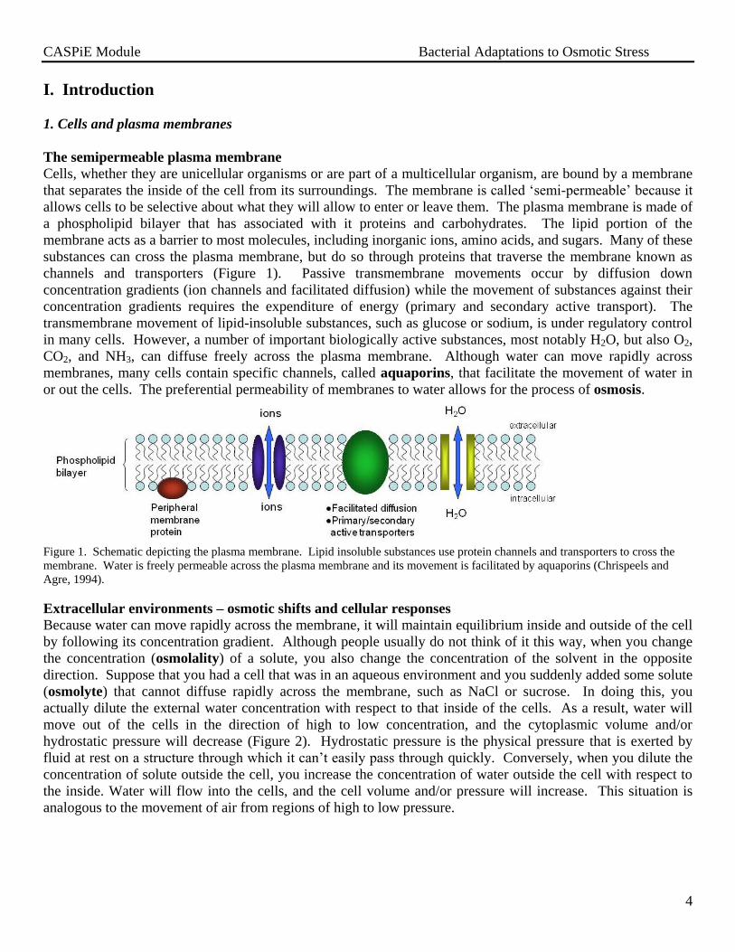
channels and transporters (Figure 1). Passive transmembrane movements occur by diffusion down
concentration gradients (ion channels and facilitated diffusion) while the movement of substances against their
concentration gradients requires the expenditure of energy (primary and secondary active transport). The
transmembrane movement of lipid-insoluble substances, such as glucose or sodium, is under regulatory control
in many cells. However, a number of important biologically active substances, most notably H2O, but also O2,
CO2, and NH3, can diffuse freely across the plasma membrane. Although water can move rapidly across
membranes, many cells contain specific channels, called aquaporins, that facilitate the movement of water in
or out the cells. The preferential permeability of membranes to water allows for the process of osmosis.
Figure 1. Schematic depicting the plasma membrane. Lipid insoluble substances use protein channels and transporters to cross the
membrane. Water is freely permeable across the plasma membrane and its movement is facilitated by aquaporins (Chrispeels and
Agre, 1994).
Extracellular environments – osmotic shifts and cellular responses
Because water can move rapidly across the membrane, it will maintain equilibrium inside and outside of the cell
by following its concentration gradient. Although people usually do not think of it this way, when you change
the concentration (osmolality) of a solute, you also change the concentration of the solvent in the opposite
direction. Suppose that you had a cell that was in an aqueous environment and you suddenly added some solute
(osmolyte) that cannot diffuse rapidly across the membrane, such as NaCl or sucrose. In doing this, you
actually dilute the external water concentration with respect to that inside of the cells. As a result, water will
move out of the cells in the direction of high to low concentration, and the cytoplasmic volume and/or
hydrostatic pressure will decrease (Figure 2). Hydrostatic pressure is the physical pressure that is exerted by
fluid at rest on a structure through which it can’t easily pass through quickly. Conversely, when you dilute the
concentration of solute outside the cell, you increase the concentration of water outside the cell with respect to
the inside. Water will flow into the cells, and the cell volume and/or pressure will increase. This situation is
analogous to the movement of air from regions of high to low pressure.

CASPiE Module Bacterial Adaptations to Osmotic Stress
5
Figure 2. Illustration of cellular response to an
increase in environmental osmolality. Water
will move out of the cell through water channels
to bring the water balance inside and outside of
the cell back into equilibrium.
Because of the high permeability of membranes to water, very early during the evolution of life, cells needed to
acquire regulatory mechanisms that enabled them to cope with fluctuations in the external osmolality.
Universally, cells adapt to increases in external osmolality by accumulating the so-called compatible solutes,
whose function is to maintain the proper balance between the external and internal water concentration.
Compatible solutes can be accumulated by de novo biosynthesis or by transport from the outside. In response
to decreases in external osmolality, solutes are rapidly released from the cell to regain the proper water balance
and cell volume (Figure 3).
Figure 3. Response of cells to changes in external
osmolality. Illustrated are the paths for the uptake and
synthesis of compatible solutes as well as paths for transport
of solutes out of the cell and free water movements.
Biological Significance of Osmoregulation
The regulation of intracellular osmolality is fundamental to physiological functions of all organisms. For
example, the mammalian kidney can extract water from the urine, resulting in up to 4-fold higher concentration
of membrane-impermeable solutes than in the blood plasma. The ability of the kidney to accomplish this
depends on the fact that the nephrons are surrounded by renal medullary cells (Figure 4 Left) whose cytoplasm
is maintained at a higher tonicity than the plasma by the accumulation of compatible solutes, such as glycine
betaine (N,N,N-trimethyl glycine) (Russell et al., 2008). As an animal experiences dehydration or excessive
hydration, the tonicity of the urine changes, and the renal medullary cells must be able to regulate their internal
osmolality accordingly. In vascular plants, the movement of water from the soil into the roots, into the xylem,
into the leaves, and then into the atmosphere in transpiration (a useful image can be found at
http://www.ncbi.nlm.nih.gov/bookshelf/br.fcgi?book=mcb&part=A4493) is determined by a progressive decrease in extracellular water,
which must be maintained by proper osmotic adjustment at each intermediate step (Salisbury and Ross, 1991).
With drought or increase in the osmolality of the water in the soil, the plants also need to regulate the osmolality

CASPiE Module Bacterial Adaptations to Osmotic Stress
6
of cells in each tissue in order to maintain the flow of water from the soil to the atmosphere. Bacteria can
encounter a variety of external environments during their lifetime and also exhibit the universal osmoregulatory
responses. Surprisingly, in the bacterium Salmonella typhimurium, adaptation to high osmolality involves a
regulatory response that greatly increases the thermotolerance of the bacteria by an unknown mechanism
(Cánovas et al., 2001). Because heat treatment is the most widely used and cost effective means for inactivating
pathogens in food products, the study of osmoregulation in Salmonella therefore has important practical
applications to food microbiology.
Figure 4. Illustration of a system that is dependent on osmoregulation for their function. A section through a human kidney showing
the nephron (functional unit of the kidney) much of which is surrounded by medullary cells which work together in osmoregulation. Image from: http://kidney.niddk.nih.gov/kudiseases/pubs/yourkidneys/ :
2. Bacteria as model organisms in the study of osmoregulation
Because of the common descent of living organisms, many basic processes and pathways are conserved
between seemingly different organisms such as bacteria in the gut (Bacterial Kingdom) and humans (Eukarya
Kingdom) (Figure 5). A conserved structure or process means that it is found in a variety of different life forms
in a very similar, if not identical, form.
Figure 5. A diagram illustrating the organization of life
into 3 Kingdoms. Note that all 3 kingdoms arise from a
single point and diverge to comprise bacteria, archaea,
and eukarya. These kingdom divisions are based on the
sequence and type of ribosomal RNA. Despite the
indication of Halobacteria and Methanobacteria in
Kingdom Archaea, these are not the same as organisms
comprising Kingdom Bacteria. All three Kingdoms are
considered equally different from the other two. Image
from: http://rst.gsfc.nasa.gov/Sect20/phylogenetictreeoflife.jpg

CASPiE Module Bacterial Adaptations to Osmotic Stress
7
While some specific features differ between cells of different organisms, like the presence of membrane-bound
organelles and nucleus, all cells maintain an internal environment which is different in a variety of ways from
the external environment in which they live. This is a function of the semi-permeable plasma membrane in all
types of cells from bacteria to eukaryotic animal and plant cells and the cell wall together with the plasma
membrane in eukaryotic fungi and plant cells (Figure 6). It is important to note that the cell wall in bacteria and
plant cells is also a physical barrier and offers rigid structural support for the cell to support the hydrostatic
pressure inside the cells.
Figure 6. Comparison of the basic structural features of
bacterial, animal, and plant cells. Image from :
www.exploringnature.org
Regardless of the organism, the balance of critical substances such as nutrients, ions and water is maintained
across all kingdoms of life with the use of integral membrane proteins that mediate the movement of
membrane-impermeant substances into and out of the cells. Not only are the membrane proteins similar in
general function in all cells, but they are phylogenetically related at the level of the gene (region of the genetic
material coding for a protein and regulation of its expression). These types of genes are referred to as highly
conserved because they encode for proteins that carry out processes so critical for survival of all organisms that
they have been kept largely unchanged over the course of evolution from single-celled organisms to large,
multicellular organisms like ourselves. Examples include P type ATPases (some Ca++
ATPases, the Na+/K
+
ATPase, H+ ATPase, etc), some potassium channels, sugar transporters, water channels, and enzymes of central
metabolism (Kühlbrandt, 2004; Loukin et al., 2005; Davidson et al., 2008; Kruse et al., 2006; Caetano-Anollés
et al., 2009).
Oftentimes when biologists wish to understand a process or function better or manipulate it, a model organism
is used for study. A model organism is one that exhibits the structures or physiological responses of interest,
but has some attributes that make it easy for scientists to study them. Common model systems include yeast,
bacteria (especially Escherichia coli and S. typhimurium), worms known as Caenorhabditis elegans, the fruit
fly Drosophila melanogaster, and mice. These organisms have attributes that are desirable in an experimental
system such as small size, well-defined structures and functions, short life cycles, ease of genetic analysis, and
easy maintenance in a laboratory setting. One specific advantage is that the sequence of the entire genome in
each of these model organisms is known, so scientists can track mutations (changes) in the genomes. Changes
in the genetic material have the potential to alter the structure or function of the organism.
In most bacteria, including S. typhimurium, the major compatible solutes are glycine betaine and the amino acid,
proline. In keeping with the universal nature of cellular osmoregulation, the same two compounds are
synthesized as compatible solutes by a wide variety of plants, and glycine betaine is used for the same function

CASPiE Module Bacterial Adaptations to Osmotic Stress
8
by mammalian kidney medullar cells. One way S. typhimurium accumulates proline and glycine betaine to high
concentration in response to high osmotic stress is by uptake from the medium via the ProP transport protein
(Figure 7). The uptake of glycine betaine and proline by ProP is driven with the expenditure of metabolic
energy (secondary active transport), which makes it possible to accumulate these substances inside the cells at
over 1000-fold higher concentration than outside.
Figure 7. Cellular response to high extracellular osmolality. Cells maintain proper water balance and volume by the uptake of
compatible solutes. In bacteria such as E. coli and S. typhimurium, proline and glycine betaine are taken up from the environment via
the ProP transporter protein in the plasma membrane. Rectangles represent impermeable osmolytes and red circles represent
compatible solutes.
The ProP protein is osmotically regulated, so that high osmotic stress results in a 10-fold increase in its activity
(Dunlap and Csonka, 1985). The ability to respond to activation by osmotic stress has been built into the ProP
protein itself, but the features of ProP that determine its ability to sense and to respond to osmotic stress are not
known (Wood, 2007). One of the main goals of the Csonka laboratory is to contribute to the elucidation of the
regulation of the adaptive mechanisms to osmotic stress in organisms. In this module, the students will study
the mechanism of the regulation of the ProP protein of S. typhimurium by isolating and characterizing mutations
that result in alterations in its functional regulation.
3. Summary of what isn’t known
Osmolality is a physical rather than a chemical signal. Although we have a fairly comprehensive knowledge of
the cellular responses that are regulated by osmotic stress in bacteria, plants, and animals, our understanding of
what the osmotic signal receptors are and how these sense osmotic stress is very inadequate. Some possibilities
are outlined in Figure 8. For example, is the signal to increase the activity of ProP uptake of compatible solutes
a direct detection of the osmotic disturbance? A result of a mechanical distortion of the protein in response to
cell shrinkage subsequent to the water efflux? Regulation of ProP function by another protein that is sensitive
to the osmotic disturbance or change in cell shape (not shown)? Or some combination of them all?

CASPiE Module Bacterial Adaptations to Osmotic Stress
9
Figure 8. Possible scenarios for increasing
uptake of compatible solutes by ProP in
response to an increase in extracellular
osmolality.
In addition to the questions regarding the detection of the high osmotic stress and the signaling to ProP to
increase its transport activity, the actual means by which this increased/altered activity is accomplished are also
not well-understood. Is it due to an increased affinity for the compatible solutes to be transported by the ProP
protein itself or is there some regulation of ProP that is modulated by osmotic stress?
Exploring these questions by analyzing the mechanisms of regulation of the ProP protein in S. typhimurium will
have applications in fields ranging from kidney physiology to agriculture and food microbiology.
4. Module Calendar
This module is organized to take you through the process of isolating bacteria that are able to survive under our
experimental conditions and to determine what underlies this ability at the genetic and protein levels. To this
end, you will learn how to work with bacteria using sterile aseptic technique and how to perform mutagenesis,
mutation mapping, and gene sequencing using PCR and online databases to characterize the bacteria. This
work will culminate in the communication of your results in the form of a research poster. The general outline
of the weekly activities can be seen in Table 1.

CASPiE Module Bacterial Adaptations to Osmotic Stress
10
Table 1. Outline of weekly lab module activities and outcomes.
Lab
session
Culturing
bacteria and
aseptic
technique
Mutagenesis Mapping
mutations
Sequencing
mutations
Data analysis
and
presentation
Outcomes
1-3 Learn
requirements
for growth and
maintenance of
a pure culture
Learn about
basic genetics
1- Become
proficient working
with bacterial
cultures
2- Understand ProP
transport system
3-Learn about
hypothesis –driven
inquiry
4 and 5 Perform
mutagenesis
and select
mutants
1- Learn how to
select mutants
6-11 Learn
transduction
technique and
about genetic
linkage and its
use in mapping
mutations
1- Become familiar
with mutation
mapping and
selection
2- Use generalized
transduction as a
molecular
biological tool
12 and
13
Learn PCR and
agarose gel
electrophoresis
1- Amplify and
sequence the ProP
gene with PCR
2- Learn how to run
an agarose gel
14-15 Learn how to
organize results
in poster
format
1- Learn data
handling, analysis,
and presentation
skills
2- Answer a
research question
5. What is the Big Picture?
In addition to learning important basic Biology laboratory skills and techniques, this module will give you the
opportunity to do real scientific experiments and to participate in a real research project. You will perform a
mutagenic screen to generate unique, never-before-seen mutants that will be mapped and sequenced.
Throughout this process, you will be generating mutants that will be valuable strains for current research aimed
at identifying the mechanisms of ProP function in general and in response to osmotic stress conditions. As
such, the data you collect will be incorporated into the research project of the Csonka lab and may be reported
in a professional scientific journal where you will be officially recognized for your contribution. You will also
report your data in the form of a scientific poster session at the end of the semester. If you have an interest in
science or want to pursue a scientific career, participating in a real research project is a great experience, and
you will learn important concepts that you can take with you for the remainder of your Biology education and
beyond.

CASPiE Module Bacterial Adaptations to Osmotic Stress
11
II. Laboratory Period 1 - Illustration of the physical process of osmosis, designing
experiments, and introduction to aseptic technique
Objectives
At the end of this laboratory period the students will be able to:
1. Understand the physical process of osmosis
2. Employ the scientific method to answer a question
3. Gather and organize data
4. Properly use a micropipette
5. Use a balance
6. Understand the importance of aseptic technique
7. Utilize aseptic technique in the transferring of solutions
1. Introduction
In the introduction to this module, you were presented with information about the importance of regulating cell
volume and shape for the proper functioning of an organism (single-celled organism) or portions of an
organisms (multicellular organisms). As cells encounter varying osmotic environments they will either take on
or lose water via osmosis. To minimize these changes cells will accumulate or get rid of compatible solutes.
Bacteria are a simple model system in which to study this response and to examine adaptive changes that they
can employ in the form of genome modifications. In order to explore this fundamental response to
environmental osmotic changes in bacteria, we need to learn how to logically approach answering scientific
questions, to understand osmosis, and to learn how to work with bacteria.
A. Introduction for Part 1 of the Procedures:
Exploring the physical process of osmosis.
In order to understand how dissolved substances in the internal and external aqueous environments of cells
influence their structure and function, we need to develop some vocabulary to describe the absolute and relative
composition of these two solutions. Cells contain an aqueous internal environment, the cytosol, in which many
substances are dissolved. The immediate external environment of living cells is also aqueous, but can have a
very different composition. The concentration of dissolved substances (solutes) in a liter of liquid (solvent) is
known as the osmolarity of the solution with units of osmoles solute/ liter solvent. Another measure of the
amount of solute dissolved in a solution is osmolality which is osmoles solute/ kilogram of solvent. This
measure is similar to osmolarity in general concept, but is more precise in that it takes away any temperature-
dependent changes in the volume of solvent.
When a cell is placed into a solution, it will lose or gain water dependent on a quantity called the water
potential (Ψ). Water potential is the potential that water has to move across a semi-permeable membrane, such
as that of a cell in solution, based on difference across the membrane. The two primary quantities that
determine the water potential across a membrane are pressure potential and solute potential on each side of the
membrane. Water potential is calculated as the total sum of pressure potential (Ψp) and solute potential (Ψπ).
(Equation1)
Pressure potential is the potential determined by the physical pressure of enclosed fluid inside a cell pushing out
and fluid outside a cell pushing in on the enclosed solution (Figure 1). An important function of this pressure
can be observed in plants where the cell must be turgid in order to support the plant and the cell wall is
structurally rigid. As water enters the cell, pressure potential goes up, since there is more force exerted by the
greater volume onto the cell wall. When a plant cell is filled with a greater quantity of water, the pressure
CASPiE Module Bacterial Adaptations to Osmotic Stress
12
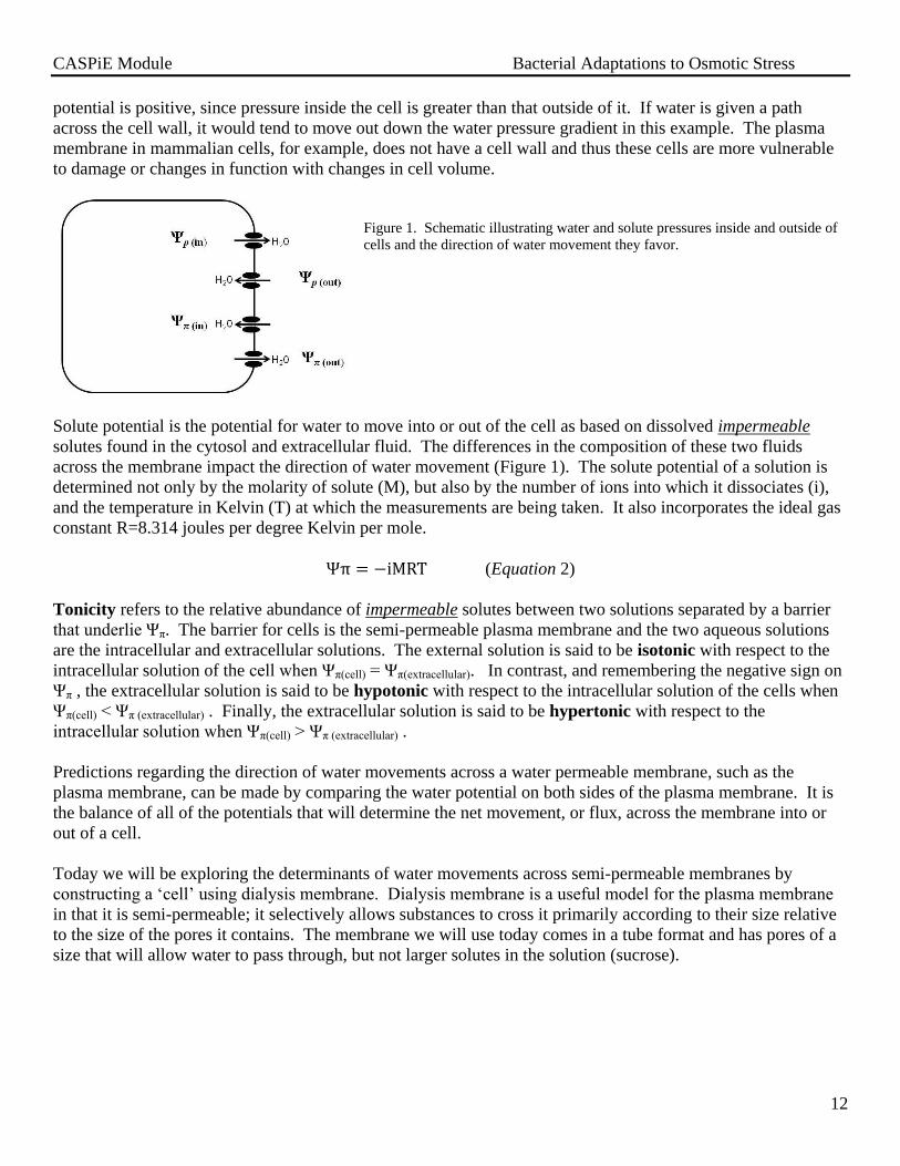
potential is positive, since pressure inside the cell is greater than that outside of it. If water is given a path
across the cell wall, it would tend to move out down the water pressure gradient in this example. The plasma
membrane in mammalian cells, for example, does not have a cell wall and thus these cells are more vulnerable
to damage or changes in function with changes in cell volume.
Figure 1. Schematic illustrating water and solute pressures inside and outside of
cells and the direction of water movement they favor.
Solute potential is the potential for water to move into or out of the cell as based on dissolved impermeable
solutes found in the cytosol and extracellular fluid. The differences in the composition of these two fluids
across the membrane impact the direction of water movement (Figure 1). The solute potential of a solution is
determined not only by the molarity of solute (M), but also by the number of ions into which it dissociates (i),
and the temperature in Kelvin (T) at which the measurements are being taken. It also incorporates the ideal gas
constant R=8.314 joules per degree Kelvin per mole.
(Equation 2)
Tonicity refers to the relative abundance of impermeable solutes between two solutions separated by a barrier
that underlie Ψπ. The barrier for cells is the semi-permeable plasma membrane and the two aqueous solutions
are the intracellular and extracellular solutions. The external solution is said to be isotonic with respect to the
intracellular solution of the cell when Ψπ(cell) = Ψπ(extracellular). In contrast, and remembering the negative sign on
Ψπ , the extracellular solution is said to be hypotonic with respect to the intracellular solution of the cells when
Ψπ(cell) < Ψπ (extracellular) . Finally, the extracellular solution is said to be hypertonic with respect to the
intracellular solution when Ψπ(cell) > Ψπ (extracellular) .
Predictions regarding the direction of water movements across a water permeable membrane, such as the
plasma membrane, can be made by comparing the water potential on both sides of the plasma membrane. It is
the balance of all of the potentials that will determine the net movement, or flux, across the membrane into or
out of a cell.
Today we will be exploring the determinants of water movements across semi-permeable membranes by
constructing a ‘cell’ using dialysis membrane. Dialysis membrane is a useful model for the plasma membrane
in that it is semi-permeable; it selectively allows substances to cross it primarily according to their size relative
to the size of the pores it contains. The membrane we will use today comes in a tube format and has pores of a
size that will allow water to pass through, but not larger solutes in the solution (sucrose).

CASPiE Module Bacterial Adaptations to Osmotic Stress
13
Testing hypotheses
One of the goals of this course is to give you the opportunity to make observations of/learn about the
physiology and functioning of bacteria and ask questions regarding them in the form of experiments. One of
the important ways in which scientists learn about the subject they are interested in is by employing what is
called the scientific method. This approach to research is comprised of six basic parts:
1. Observe a phenomenon
2. Formulate a question about your observation
3. Design a testable hypothesis based on your observations and previous knowledge to explain the phenomenon
or answer your question
4. Use the hypothesis to make predictions
5. Design and carry out experiments to test the predictions of the hypothesis
6. Compare the results of the experiment to your predictions
7. Accept hypothesis or modify it and repeat steps 3-5
Example:
You observe that your dog always gets its “favorite smooth red ball” when you grab the leash to go for a walk.
A question you might have is why does your dog like that particular ball? You hypothesize that your dog really
likes the color red. You predict that your dog will not play with a ball of a different color. The next day you
experiment and put a yellow tennis ball next to the red one before your walk. As you predicted, you observe
that your dog chooses the red ball over the yellow ball. You conclude that your hypothesis was supported by
your data.
An important component of each experimental plan is the design of controls. Controls are as important to the
experiment as the experimental manipulation itself! In the example above the alternative to the smooth red ball
was a yellow tennis ball. It’s possible that the reason why your dog didn’t take the tennis ball was because it
actually liked the smooth texture of the red ball and not the color. One possible control for this experiment
would be to use a red tennis ball. Can you think of another one? A control should ideally be identical to your
experimental manipulation in all attributes except the one of interest. Good controls are not always easy to
design but should always be attempted otherwise it is difficult to interpret your data.
Once hypotheses have been experimentally tested and consistently supported by the data, they become theories.
A theory is the accepted explanation of a phenomenon or process based on supportive evidence. It can,
however, be revised or discarded if new data accumulate that do not support the theory and the hypotheses that
underlie them. It is very difficult, in science, to prove something definitively!
Working definitions for our class:
Hypothesis – This is a take-a-stand statement based on your observations/knowledge regarding the way
something works. You can think about it as an answer to a question (What is your dog’s favorite ball color?).
Avoid statements that are predictive in nature. For example: Red is my dog’s favorite color for a ball. Note
the use of the word ‘is’. It’s fine if your results don’t support your initial hypothesis!
Prediction – This is where you can express some conditionality or uncertainty (if…then).

CASPiE Module Bacterial Adaptations to Osmotic Stress
14
B. Introduction for Part 2 of the Procedures:
Measuring small volumes using Micropipettes
One of the most useful instruments that you will use in many laboratory settings is the Micropipette. The
Micropipette allows you to obtain and dispense very small quantities (<1 mL) of liquid accurately and quickly.
Micropipettes come in different sizes calibrated to be useful in a particular range of volumes (Table 1).
Table 1. Volume ranges for selected micropipettes
Micropipette Volume range Acurate volume range
P-20 0-20 μl 2-20 μl
P-200 0-200 μl 50-200 μl
P-1000 0-1000 μl (0.1 – 1 mL) 100-1000 μl
Figure 2. Standard micropipette and useful features. Image from: http://commons.wikimedia.org/wiki/File:Manual_microliterpipette.jpg
An example of what a Micropipette looks like showing its important features can be seen in Figure 2. The size
of the micropipettes can be found on the micropipette plunger (A). While the micropipettes are rated for use
over a large range of volumes, they are most accurate in the middle of their range (see table 1). For example,
while P-1000, P-200, and P-20 can all be set to draw up and dispense 5 μl they are not all equally accurate
handling this small volume. In general, a good rule of thumb is to use the smallest range Micropipette possible
for the volume you are working with so the volume is in the middle range (ie., to work with 150 μl of solution
use the P200 micropipette instead of the P1000 micropipette). To set the volume to be drawn up and dispensed,
rotate the micrometer dial near the top of the micropipette (B) and move it until the desired volume appears in
the window on the side of the micropipette (not shown on this image). Figure 3 illustrates examples of setting
volumes for the P-1000, P-200, and P-20 micropipettes.

CASPiE Module Bacterial Adaptations to Osmotic Stress
15
Figure 3. Example volume settings for P-1000, P-200, and P-20
micropipettes. The window on the side of each micropipette displays
a volumeter that is set to the desired volume. The number places for
each micropipette with an example are shown.
You will always use disposable tips that you affix to the end of the micropipette (C) that actually hold the liquid
you are working with. Oftentimes you will be changing the tip with every volume that you move and you will
remove the tip using the ejector button at the top of the micropipette (D). Tips will be provided to you as well
as a waste receptacle to place them in when you are finished.
In order for micropipettes to be useful to us, they need to be used with care and periodically calibrated. This is
done by drawing up and weighing a volume of fluid with a known density. Distilled water has a density of
1gram/ 1 mL and provides us with a convenient fluid to practice accurately using the micropipettes. We will be
using water today to practice using micropipette accurately (actual and expected results are close) and
precisely (repeatability; each time you do it there is little variation).
C. Introduction for Part 3 of the Procedures:
Introduction to aseptic technique
Microorganisms are found everywhere. They are an incredibly diverse group of organisms, some of which have
adapted the ability to grow in environments with temperatures over 200°F or below -17°F, with pH values
below 0 and above 11.5, and with extreme salinity up to saturation. Given the ability to grow in such extreme
environments, it should come as no surprise that microbes can exist in all locations including the lab bench, the
air ducts, and your fingers. Because of this, great care must be taken to make sure the only organisms that get
into your nutrient-rich growth media is the bacterial culture you intend to grow up. To ensure this is the case,
microbiologists employ the use of aseptic technique when working with cultures of bacteria. Aseptic
technique involves sterilizing the containers holding the bacteria of interest and anything that may come into
contact with them most often by flame sterilization. In addition to keeping the bacterial culture
uncontaminated, using aseptic technique also keeps the experimenter and their workspace uncontaminated with
the bacteria as well!
2. Pre-laboratory activities
Read the introduction and the procedures for Laboratory Period 1 in this section of the lab manual. Where
indicated in the procedures sections in bold, work out calculations for any solutions to be made or diluted.
Before the lab period log onto Blackboard and take the pre-lab quiz for this week.
Osmosis experiment – You will be using this experiment to practice the process of scientific inquiry and to
explore osmosis. To this end, you will work with your group to work through the scientific method. In your
laboratory notebook write out the following questions/topics and your answers or responses:
a. What do you know about the determinants of water movements across semipermeable membranes?
b. Design hypotheses for water movements across a semipermeable membrane for a cell placed in isotonic vs.
hypotonic vs. hypertonic solutions.
c. Predict changes in cell volume and weight in the three tonicity scenarios.

CASPiE Module Bacterial Adaptations to Osmotic Stress
16
Carry out the experiment to test your hypotheses according to the procedure outlined below.
3. Materials
For examination of the physical process of osmosis:
Equipment and materials
● Sucrose
● Dialysis tubing
● Scissors
● Large beaker in which to hydrate dialysis tubing
● Gloves
● Paper towels
● Dialysis tubing closures (6/group)
● 3, 500 ml beakers/group
● 1, 100 ml beaker/group
● deionized H20
● labeling tape
● sharpies
● weigh boat to sit on balance
● balance
● 3, 4 L erlenmyer flasks to hold prepped solutions
Reagents
● Solution A (isotonic solution = X = 5% sucrose solution)
● Solution B (hypotonic solution = deionized water)
● Solution C (hypertonic solution = 20% sucrose solution)
● Solution X (intracellular solution = 5% sucrose solution)
Measuring small volumes using Micropipettes:
Equipment and materials
● P-1000 micropipette
● P-200 micropipette
● P-20 micropipette
● P-1000 tips (blue)
● P-200 tips (yellow or clear)
● P-20 tips (small clear)
● Balance
● Weigh paper
● Small beaker of distilled water
● Micropipette tip waste receptacle.
For general aseptic technique
Equipment and materials
● Four test tubes filled with 5 ml of sterile LB media per person
● P-1000 micropipettes
● P-1000 pipette tips (sterile)
● Sharpies
● Bunsen burners
CASPiE Module Bacterial Adaptations to Osmotic Stress
17
● Strikers
● 37°C shaking incubator
Reagents
● Sterile LB media
4. Procedures
Part 1: Osmosis
1. Please obtain from the front desk:
i. a pair of gloves
ii. Three (3) pieces of dialysis tubing (it is critical that you wear gloves any time you handle
the dialysis tubing as the oil on your fingers can clog the pores in the membrane)
iii. Six (6) dialysis closures (2 each of closures labeled A, B, and C)
iv. One (1) small beaker labeled ‘X’ (intracellular fluid)
2. Close one end of a length of tubing near an end with one of the A closures making sure that the clip snaps
shut and that some tubing is sticking out from the clip.
3. Open the end of the tubing by gently rubbing it together between your fingers.
4. Fill the tubing ¾ full with solution from the small beaker (solution X). To get the filling started, it helps to
put the tip of your finger in the opening and slowly pour the fluid along that finger into the tubing.
5. Remove any large air bubbles from the tubing.
6. Close the other end of the tubing with the other A closure close to the end with some tubing sticking out of
the clip.
7. If constructed properly, your ‘cell’ should have some space in it, but not air. You can test this by gently
pinching the ‘cell’ between two of your fingers. You should be able to touch your fingers together across the
cell.
8. Put that ‘cell’ on a paper towel on the bench and repeat steps 2-7 for ‘cells’ B and C.
9. Gently dry off your three ‘cells’ and take them to the balance to weigh. Remember to tare the balance
between each cell.
10. Weigh each ‘cell’ and record this baseline weight in your lab notebook
11. Get three (3) solution-filled beakers (A, B, and C) from the front table.
12. Place each ‘cell’ in their appropriate beaker (Ex. ‘cell’ with A clips in the A beaker) and note the time.
13. After ~60 minutes have elapsed mark the time in your lab book, take your ‘cells’ out of their beakers, dry
them, and record their post experiment weight in your lab notebook.
14. Compare the trends in your experimental data with what you and your group predicted would happen to the
cell volume (as measured by weight) when placed in isotonic, hypertonic, or hypotonic extracellular solutions.
15. Gather the data from all of the lab groups to analyze.
Part 2: Measuring small volumes using Micropipettes – We will demo this for you first
At your station you will find 3 micropipettes (P-20, P-200, and P-1000) as well as disposable tips for each of
them autoclaved (steam sterilized) and boxed for you. You will also find a small beaker of distilled water. You
will practice using the micropipettes today by drawing up and weighing varying volumes of distilled water.
Before doing so, please read and remember the following guidelines:
● Never rotate the volume control dial past its maximum/minimum value
● Never draw up liquid without a disposable tip in place
● Always work the plunger slowly
CASPiE Module Bacterial Adaptations to Osmotic Stress
18
● Never place a micropipette in a horizontal position while fluid is in the tip; this fluid could enter the
micropipette and damage it
● Never immerse the micropipette itself into fluid
Each member of your lab group will be measuring the following volumes:
5 μl 200 μl
10 μl 250 μl
20 μl 500 μl
50 μl 1000 μl
100 μl
1. In your lab notebook construct a data table to record the volume to be measured, micropipette used, the
predicted weight of each volume, and weight measured for each volume (in triplicate). What is the
smallest volume of water that can be weighed on our balances?
2. Place a weigh boat on the analytical balance and zero (tare) the balance
3. Obtain the appropriate micropipette to transfer 1000 μl of distilled water
4. Set the volume to be transferred on the micropipette by rotating the micrometer dial to 1000 μl
5. Place the appropriate disposable tip firmly on the end of the micropipette. Do this by placing the barrel in a
tip in the box, pressing it down, and then tapping it in the box.
6. Depress the plunger to the first stop. There are two stops and the first one is the first resistance you meet as
you depress the plunger. This stop is determined by the volume setting you set.
7. With the plunger still depressed to the first stop, place the disposable tip into the beaker of water
8. Slowly release the plunger and watch as the water is drawn up into the disposable tip.
9. Wait 2-3 seconds after you have fully released the plunger to allow the entire volume to be drawn up into
the disposable tip.
10. Holding the micropipette upright, move to the analytical balance.
11. Tare (zero) the balance if it has drifted from zero
12. Holding the micropipette and tip above the weigh boat*, dispense the water onto the weigh boat by slowly
depressing the plunger to the first stop.
13. After 2-3 seconds depress the plunger past the first stop to the second stop. This will force any remaining
fluid out of the disposable tip. Slowly release the plunger.
14. Record the weight of the volume of water you just dispensed.
15. Eject the micropipette tip into the tip waste receptacle by easing it off with your hand or depressing the
ejector.
16. Carefully repeat steps 2-15 two more times for 1000uL of water (you don’t need to dump the water from the
weigh boat after each volume is pipette onto it. Simply tare the balance before each addition).
17. Repeats steps 2-16 for the other volumes (500, 240, 200, 100, 50, 20, 10, and 5 μl (only one person/group
needs to do this last volume)). There are three people per group and three sizes of micropipette at each
station, how can your group efficiently move through this exercise?
18. In your lab notebook calculate and record the average weight for each volume for each person and record
this in your lab notebook. In addition, calculate the % error of each value from the average weight at each
volume. How would you calculate this? Ideally, you want your triplicates to be less than + 5% different
from the average at each volume. If your % error is higher than this, what are possible sources of error?
Consult with us to identify the issue.
*when dispensing liquid into another liquid, lower the disposable tip into the liquid in the recipient container or
touch the tip to the side of recipient container if you cannot reach the fluid. Then dispense the liquid from your
micropipette.
CASPiE Module Bacterial Adaptations to Osmotic Stress
19
It is important that you can accurately and precisely pipette small volumes of fluid for your experiments
to work this semester, so the time spent working on your technique now will be helpful later!
Part 3: General aseptic technique – We will demo this for you first
1. Obtain four test tubes containing 5 ml of sterile LB media. Two test tubes will be used for aseptic transfer
of media, and two will be used for non-aseptic transfer. Label one tube in each set “A”. This will be the
tube you transfer media from. Label the second tube in each set “B”. This will be the tube you transfer
media to.
2. Turn on the Bunsen burner.
3. Remove the cap from Clean tube A with your dominant hand and pass the tube through the flame with your
non-dominant hand. You need to keep holding the cap!
4. Using a P-1000 micropipette, pull up 1000 μl of media.
5. Pass the tube through the flame again and re-cap the tube.
6. Remove the cap from Clean tube B as you did with A and pass the tube through the flame.
7. Dispense the liquid from the micropipette into tube B.
8. Pass the tube through the flame again and re-cap the tube.
9. Repeat the procedure above with the Dirty tubes, being sure to first touch the pipet tip to any unclean
surface before pulling up or dispensing any liquid. Do not flame either of the tubes in the dirty set.
10. Incubate the test tubes at 37°C.
5. Post-laboratory analysis and results
Today each group obtained data regarding the movement of water across a semi-permeable membrane in
different osmotic conditions. You have now gathered the results from this experiment from each lab group.
How do you go about organizing the data and making claims about it and your hypotheses?
● Draw qualitative conclusions about the data set and record them in your lab notebook (3-4 sentences)
● Compare the trend in your group’s data set to that of the class data set and summarize the comparison in your
lab notebook (3-4 sentences)
● Find the average weight change of the cell in each condition and record them in your lab notebook
● Graphically represent the results from the whole group by hand in your lab notebook in at least two different
formats
6. Preparation for the Next Laboratory Activity
● You should read the introduction and procedures for Laboratory 2 before going to your next laboratory
period.
● Perform any calculations and answer any questions as indicated in bold in the Laboratory 2 text.
● Take the online pre-lab quiz by midnight on Tuesday, January 18th
.

CASPiE Module Bacterial Adaptations to Osmotic Stress
20
III. Laboratory Period 2 – Quantitative data analysis methods, independent dilutions,
preparation of solid bacterial growth media, and methods of plating bacteria
Objectives
At the end of this laboratory period the students will be able to:
1. Understand differences between and uses of qualitative and quantitative data analyses
2. Use descriptive and test statistics to interpret their data
3. Clearly communicate their data in graphical form
4. Understand the importance and use of bacterial growth media in microbiological research
5. Perform calculations used in making molar solutions
6. Perform dilutions from stock solutions
7. Properly use a graduated cylinder
8. Follow a recipe for preparing media
9. Understand the use of autoclaving for sterilizing media
10. Utilize aseptic technique in the pouring of plates and transferring solutions
11. Understand the importance of isolated colonies in microbial research
12. Use an inoculating loop for streaking bacteria on plates
13. Perform quadrant streaking for isolated colonies
14. Use a hockey stick spreader to spread plate bacteria
15. Explain the pros and cons of quadrant streaking versus spread plating bacteria
Examine media transfer tubes for contamination
1. Introduction
Being able to organize data sets, interpret them, and clearly display them for others to understand are essential
skills for all scientists. Both qualitative and quantitative data analyses assist scientists in understanding their
experimental results and planning their next step. Today we will be assisting you in making sense of the data
we collected from our osmosis experiment last week and organizing it into a clear graphical form that will
clearly communicate the results to the group.
Pure culture technique is an essential tool for the study of microorganisms. Bacteria of all kinds of different
species are able to grow in a multitude of locations in close proximity to one another. Not only do they grow
together, they also interact with each other to both positively and negatively affect each other’s growth.
Because of this, it is difficult to effectively study a bacterial species grown in a mixed culture with other
species. It is much easier to study an individual bacterial species grown in a pure culture containing only that
bacterial species. Today we will be making our own bacterial culture plates to grow our bacteria on and
learning two common techniques used to obtain a pure culture of bacteria, quadrant streaking for isolated
colonies and spread plating.
A. Quantitative analysis and display of data
Qualitative versus quantitative analysis
Last week you conducted an experiment to investigate the determinants of osmotic water movement using
dialysis tubing and sucrose solutions of varying tonicities. Scientists can summarize their findings with
qualitative observations of general trends in their data and precise quantitative descriptions and comparisons.
Qualitative data analyses are useful, but can be subjective, and are usually a first step in interpreting data and
guide scientists in the direction of what aspect of their data set to precisely quantify. This quantitative analysis
CASPiE Module Bacterial Adaptations to Osmotic Stress
21
of results is more objective and will make them more credible to peer scientists and others who read their
papers.
Qualitative analysis and conclusions regarding data tend to be broad descriptions of the data. As the name
suggests, the statements reflect the quality of the data. For example, a qualitative statement about the data
obtained in the osmosis experiment could be that ‘cells in the hypertonic condition were larger than cells in the
isotonic condition at the end of the incubation period’. This is a useful observation of the trend, and leads to the
quantitation of precisely how much weight cells gained or lost that underlies this appearance.
Scientists use a variety of means to quantify and make definitive statements about their data that generally fall
under two categories: (1) descriptive statistics and (2) test statistics.
Statistics - Descriptive statistics
Descriptive statistics are a first quantitative step in data analysis and typically consist of condensing data sets
down to a measure that represents the data set as a whole that will allow quick comparisons between data sets to
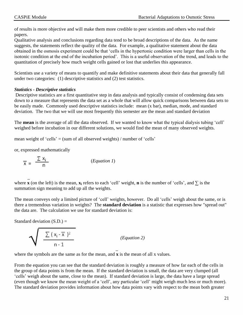
be easily made. Commonly used descriptive statistics include: mean (x bar), median, mode, and standard
deviation. The two that we will use most frequently this semester are the mean and standard deviation
The mean is the average of all the data observed. If we wanted to know what the typical dialysis tubing ‘cell’
weighed before incubation in our different solutions, we would find the mean of many observed weights.
mean weight of ‘cells’ = (sum of all observed weights) / number of ‘cells’
or, expressed mathematically
(Equation 1)
_
where x (on the left) is the mean, xi refers to each ‘cell’ weight, n is the number of ‘cells’, and ∑ is the
summation sign meaning to add up all the weights.
The mean conveys only a limited picture of ‘cell’ weights, however. Do all ‘cells’ weigh about the same, or is
there a tremendous variation in weights? The standard deviation is a statistic that expresses how "spread out"
the data are. The calculation we use for standard deviation is:
Standard deviation (S.D.) =
(Equation 2)
_
where the symbols are the same as for the mean, and x is the mean of all x values.
From the equation you can see that the standard deviation is roughly a measure of how far each of the cells in
the group of data points is from the mean. If the standard deviation is small, the data are very clumped (all
‘cells’ weigh about the same, close to the mean). If standard deviation is large, the data have a large spread
(even though we know the mean weight of a ‘cell’, any particular ‘cell’ might weigh much less or much more).
The standard deviation provides information about how data points vary with respect to the mean both greater

CASPiE Module Bacterial Adaptations to Osmotic Stress
22
than (+) and less than (-). Therefore, when reporting the mean and standard deviation it is written as mean +
S.D. For example, if the mean ‘cell’ weight is 1 gram and the standard deviation is 0.3 grams then you would
write this concisely as 1 + 0.3 grams.
Reporting the standard deviation of the data along with the mean gives a more informative picture than
reporting the mean alone. In this class you must ALWAYS report the mean + S.D. You can calculate both
statistics by using the formulas given above, but once you understand what you are doing, it will save time to
use the scientific calculator functions or spreadsheet functions for these statistics.
To understand this idea more thoroughly, look at the two sets of data below and their mean and standard
deviation to understand the importance of the standard deviation in presentation of information.
Set 1: 1.59, 3.48, 12.90, 4.20, 1.80
Set 2: 4.79, 4.28, 5.35, 4.95, 4.61
Mean 1: 4.79
Mean 2: 4.79
SD 1: 4.66
SD 2: 0.40
Although the means of the data sets may be the same, the standard deviations are vastly different. The values of
the second set are much closer to each other than those of the first set, which explains the importance of
expressing the mean with the standard deviation. Thus the mean of the first set is expressed as 4.79±2.09 and
the mean of the second set is expressed as 4.79±0.18.
Statistics – Inferential statistics (Adapted from Statistics Appendix, Janet Wright)
Inferential statistics are objective analyses that allow researchers to make statements as to whether two
experimental conditions are truly different from each other or from some expected outcome. Depending on the
type of data collected and how the experiments were designed, different tests are used. Test statistics are
numbers derived from the data that can be used to test a hypothesis. In our example, we might want to test the
hypothesis that cells take on water when placed in a hypotonic solution and cells placed in isotonic solutions do
not. The main kinds of questions that test statistics help to answer are "Are the two groups significantly
different?" and "Are the results significantly different from what I predicted?"
In the context of scientific data analysis and statistics, the term "significant" has a special meaning that is
precisely defined. To understand its basis, consider an example. Let's say you think that about 20% of college
students each breakfast in the morning. This implies that on average, one of every five people will be morning
eaters. You go out to test your hypothesis. Of the first five people you survey, four say they eat breakfast in the
morning. This is not what you predicted. Do you need to reject your hypothesis at this point? At this point you
might think that you just happened to ask four breakfast eaters by chance. You rightly intuit that you have not
gathered enough data to test your hypothesis. Now suppose you survey five thousand people, and four thousand
of them report being morning breakfast eaters. At this point you can be pretty sure that your original hypothesis
that 20% of college students eat breakfast in the morning was not supported by the data and needs to be revised.
The number of people you surveyed, also known as your sample size, is quite large and there is not a
reasonable chance that the real value is 20%.
You don't need statistics to draw a valid conclusion about your samples of five and five thousand people; five is
too small a sample size and five thousand is a sufficiently large sample size. But suppose you had sampled fifty
people, and thirty of them were breakfast eaters? Intuition is less helpful in telling you whether to reject your
original hypothesis that 20 percent of people are breakfast eaters. What you really want to know is how likely it

CASPiE Module Bacterial Adaptations to Osmotic Stress
23
is that you could get such a result in your survey even if the real proportion in the overall population is actually
20 percent as you originally thought. Now a statistical test is useful, because statisticians have already figured
out the probability that you could get a result as “off” as thirty out of fifty even when the real percentage is 20
percent. By convention, we use a 5% probability as a cutoff for accepting or rejecting a hypothesis. If the
statistic says that there's less than a 5% probability of getting thirty breakfast eaters by chance in a sample of
fifty (taken from a population where 20 percent are actually breakfast eaters), you conclude that your original
hypothesis was wrong, and you reject it. You could then report that at a 5% level of significance, your data
were significantly different from what you predicted.
When scientists analyze their data they want to know if they can accept their hypothesis or if they need to revise
or reject it. Typically in statistics, however, what is actually tested is a null hypothesis, also known as a no-
difference hypothesis, even if you think there really is a difference between two data sets. Therefore, for
purposes of conducting the statistical test, you “predict” that there will be no statistical difference in the two
data sets. If you can show statistically that your no-difference hypothesis is wrong, you can conclude that there
really is a difference between the two groups (and that your “real” hypothesis and predictions are supported by
the data).
T-test for differences between means of two samples.
The t-test is a statistical test that is used to compare data for two different samples, each of which has a mean
and a standard deviation. The values of the data points in each sample should also have what is called a
normal distribution, a shape like a bell-curve (Figure 1). In a normal distribution most data points are
clustered close to the mean and fewer and fewer data points greater than and less than the mean with 95% of
all of the data being within 2 standard deviations from the mean (Figure 2).
Figure 1. Top: Example of a normally distributed data set
with value of most of the data clustered close to the mean and
95% of the data within 2 standard deviations from the mean.
Figure 2. Graph illustrating the relationship
between the standard deviation and the mean
of a data set whose values have a bell-shaped
distribution. µ = mean and σ = standard
deviation Image By: Mwtoews [CC-BY-2.5
(www.creativecommons.org/licenses/by/2.5)], via
Wikimedia Commons
http://commons.wikimedia.org/wiki/File:Standard_devi
ation_diagram.svg
CASPiE Module Bacterial Adaptations to Osmotic Stress
24
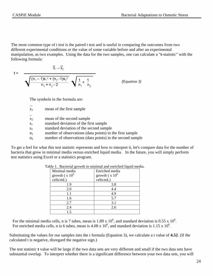
The most common type of t test is the paired t test and is useful in comparing the outcomes from two
different experimental conditions or the value of some variable before and after an experimental
manipulation, as two examples. Using the data for the two samples, one can calculate a "t-statistic" with the
following formula: (Equation 3)
The symbols in the formula are:
x1 mean of the first sample
_
x2 mean of the second sample
s1 standard deviation of the first sample
s2 standard deviation of the second sample
n1 number of observations (data points) in the first sample
n2 number of observations (data points) in the second sample
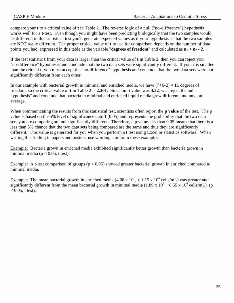
To get a feel for what this test statistic represents and how to interpret it, let's compare data for the number of
bacteria that grow in minimal media versus enriched liquid media. In the future, you will simply perform
test statistics using Excel or a statistics program.
Table 1. Bacterial growth in minimal and enriched liquid media.
Minimal media
growth ( x 106
cells/mL)
Enriched media
growth ( x 106
cells/mL)
1.9 3.8
2.0 4.4
1.1 4.9
1.6 5.7
2.7 3.1
2.4 2.6
1.5
For the minimal media cells, n is 7 tubes, mean is 1.89 x 10⁶, and standard deviation is 0.55 x 10
6.
For enriched media cells, n is 6 tubes, mean is 4.08 x 10⁶, and standard deviation is 1.15 x 10
6.
Substituting the values for our samples into the t formula (Equation 3), we calculate a t value of 4.52. (If the
calculated t is negative, disregard the negative sign.)
The test statistic t value will be large if the two data sets are very different and small if the two data sets have
substantial overlap. To interpret whether there is a significant difference between your two data sets, you will
CASPiE Module Bacterial Adaptations to Osmotic Stress
25
compare your t to a critical value of t in Table 2. The reverse logic of a null ("no-difference") hypothesis
works well for a t-test. Even though you might have been predicting biologically that the two samples would
be different, in this statistical test you'll generate expected values as if your hypothesis is that the two samples
are NOT really different. The proper critical value of t to use for comparison depends on the number of data
points you had, expressed in this table as the variable "degrees of freedom" and calculated as n1 + n2 - 2.
If the test statistic t from your data is larger than the critical value of t in Table 2, then you can reject your
"no-difference" hypothesis and conclude that the two data sets were significantly different. If your t is smaller
than the critical t, you must accept the "no-difference" hypothesis and conclude that the two data sets were not
significantly different from each other.
In our example with bacterial growth in minimal and enriched media, we have (7+6-2) = 11 degrees of
freedom, so the critical value of t in Table 2 is 2.201. Since our t value was 4.52, we "reject the null
hypothesis" and conclude that bacteria in minimal and enriched liquid media grew different amounts, on
average.
When communicating the results from this statistical test, scientists often report the p value of the test. The p
value is based on the 5% level of significance cutoff (0.05) and represents the probability that the two data
sets you are comparing are not significantly different. Therefore, a p value less than 0.05 means that there is a
less than 5% chance that the two data sets being compared are the same and thus they are significantly
different. This value is generated for you when you perform a t test using Excel or statistics software. When
writing this finding in papers and posters, use wording similar to these examples:
Example: Bacteria grown in enriched media exhibited significantly better growth than bacteria grown in
minimal media (p < 0.05, t test).
Example: A t-test comparison of groups (p < 0.05) showed greater bacterial growth in enriched compared to
minimal media.
Example: The mean bacterial growth in enriched media (4.08 x 10⁶, + 1.15 x 10
6 cells/mL) was greater and
significantly different from the mean bacterial growth in minimal media (1.89 x 10⁶ + 0.55 x 10
6 cells/mL) (p
< 0.05, t test).

CASPiE Module Bacterial Adaptations to Osmotic Stress
26
Table 2. Critical values of t for the T test at the 5% level of significance.
degrees of freedom t critical
1 12.706
2 4.303
3 3.182
4 2.776
5 2.571
6 2.447
7 2.365
8 2.306
9 2.262
10 2.228
11 2.201
12 2.179
13 2.160
14 2.145
15 2.131
16 2.120
17 2.110
18 2.101
19 2.093
20 2.086
21 2.080
22 2.074
23 2.069
24 2.064
25 2.060
26 2.056
27 2.052
28 2.048
29 2.045
30 2.042
40 2.021
60 2.000
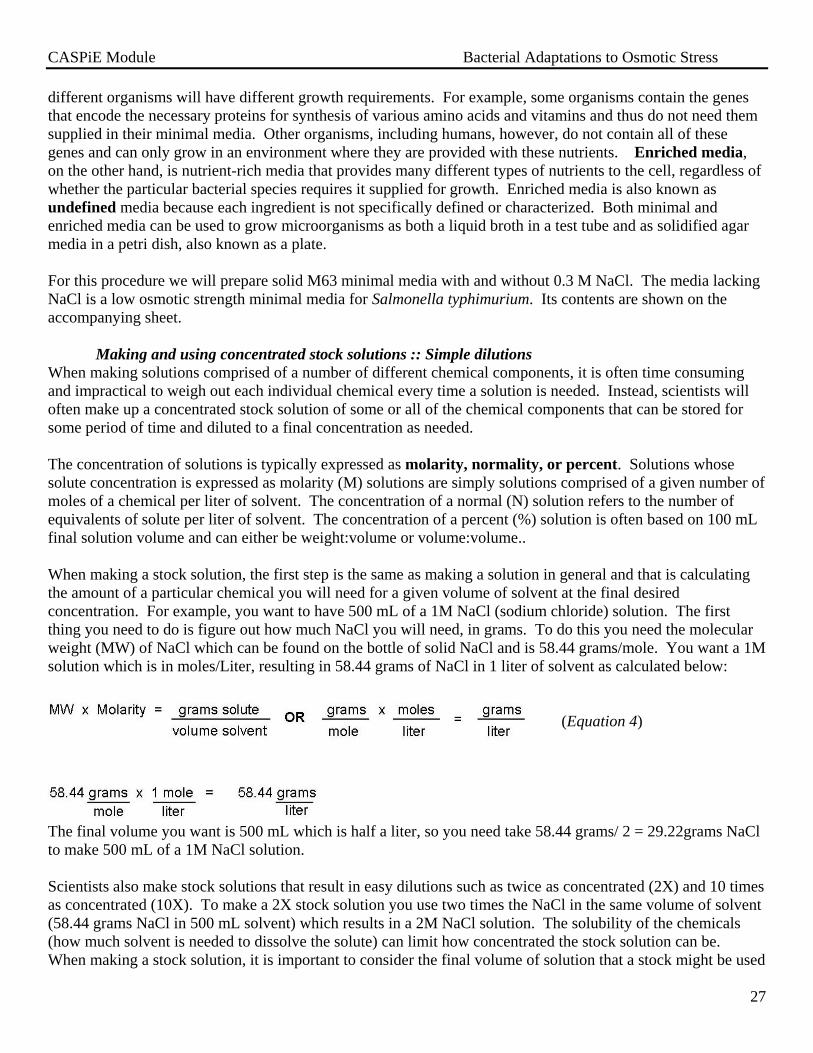
B. Introduction for Part 1 of the Procedures:
Preparation of solid minimal bacterial growth media and aseptic technique
One of the most important tools used in microbiological research is the of bacterial growth media. In order for
a bacterial species to grow successfully in a laboratory environment, its growth media must contain all the
essential components it needs. These components must include a carbon source, an energy source, a nitrogen
source, essential minerals, and possibly extra vitamins or growth factors, depending on the organism being
grown. The bacterial species being grown must be able to take up the provided nutrients into the cell and utilize
them to create necessary cell components and to produce energy used to fuel vital cell processes.
The two main categories of media used by microbiologists to grow bacterial cultures are minimal media and
enriched media. Minimal media is growth media that provides only the bare essential requirements for
bacterial growth and is also known as chemically defined media as every ingredient in the media is known by
the researcher. The type of media classified as minimal media varies amongst different bacterial species as
CASPiE Module Bacterial Adaptations to Osmotic Stress
27
different organisms will have different growth requirements. For example, some organisms contain the genes
that encode the necessary proteins for synthesis of various amino acids and vitamins and thus do not need them
supplied in their minimal media. Other organisms, including humans, however, do not contain all of these
genes and can only grow in an environment where they are provided with these nutrients. Enriched media,
on the other hand, is nutrient-rich media that provides many different types of nutrients to the cell, regardless of
whether the particular bacterial species requires it supplied for growth. Enriched media is also known as
undefined media because each ingredient is not specifically defined or characterized. Both minimal and
enriched media can be used to grow microorganisms as both a liquid broth in a test tube and as solidified agar
media in a petri dish, also known as a plate.
For this procedure we will prepare solid M63 minimal media with and without 0.3 M NaCl. The media lacking
NaCl is a low osmotic strength minimal media for Salmonella typhimurium. Its contents are shown on the
accompanying sheet.
Making and using concentrated stock solutions :: Simple dilutions
When making solutions comprised of a number of different chemical components, it is often time consuming
and impractical to weigh out each individual chemical every time a solution is needed. Instead, scientists will
often make up a concentrated stock solution of some or all of the chemical components that can be stored for
some period of time and diluted to a final concentration as needed.
The concentration of solutions is typically expressed as molarity, normality, or percent. Solutions whose
solute concentration is expressed as molarity (M) solutions are simply solutions comprised of a given number of
moles of a chemical per liter of solvent. The concentration of a normal (N) solution refers to the number of
equivalents of solute per liter of solvent. The concentration of a percent (%) solution is often based on 100 mL
final solution volume and can either be weight:volume or volume:volume..
When making a stock solution, the first step is the same as making a solution in general and that is calculating
the amount of a particular chemical you will need for a given volume of solvent at the final desired
concentration. For example, you want to have 500 mL of a 1M NaCl (sodium chloride) solution. The first
thing you need to do is figure out how much NaCl you will need, in grams. To do this you need the molecular
weight (MW) of NaCl which can be found on the bottle of solid NaCl and is 58.44 grams/mole. You want a 1M
solution which is in moles/Liter, resulting in 58.44 grams of NaCl in 1 liter of solvent as calculated below:
(Equation 4)
The final volume you want is 500 mL which is half a liter, so you need take 58.44 grams/ 2 = 29.22grams NaCl
to make 500 mL of a 1M NaCl solution.
Scientists also make stock solutions that result in easy dilutions such as twice as concentrated (2X) and 10 times
as concentrated (10X). To make a 2X stock solution you use two times the NaCl in the same volume of solvent
(58.44 grams NaCl in 500 mL solvent) which results in a 2M NaCl solution. The solubility of the chemicals
(how much solvent is needed to dissolve the solute) can limit how concentrated the stock solution can be.
When making a stock solution, it is important to consider the final volume of solution that a stock might be used

CASPiE Module Bacterial Adaptations to Osmotic Stress
28
for. Will you be using the stock to add NaCl to 100 μL or 1 L final volume? This will determine the
concentration and volume of the stock solution you make (you will need a large volume of 2X stock when
making one liter of solution).
Concentrated stock solutions can be a great time saver for researchers if they are made in convenient
concentrations for most uses in the lab and stored properly for long periods of time. Performing the appropriate
dilution of the stock is critical to take advantage of the stock solution. There are a variety of strategies that one
can use for performing dilutions that depend on the concentration of the stock solution, the final concentration
desired, and/or a specific final volume at a concentration desired.
Our 2X stock lends itself to a very simple dilution to bring it to our final working concentration of 1M. We
simply need to dilute our 2M 2X stock in half. To do this we would need to mix equal parts stock and water
(Figure 3).
Figure 3. Illustration of a simple dilution from a 2X stock solution.
Oftentimes, however, a single stock solution is used in a variety of contexts and final concentrations.
Regardless of the final concentration needed, a simple, independent volume:volume dilution is appropriate
when a single final concentration is desired. In this type of dilution, a volume of the stock solution (the aliquot)
is added to some volume of water or other solution (the diluent). By convention, the first volume in the
volume:volume expression is the aliquot volume of the stock solution being added and the second volume is the
total volume of the solution (diluent + aliquot). There are two basic scenarios encountered with volume:volume
dilutions: (1) the final concentration differs from the stock solution concentration by orders of magnitude (stock
solution is 10, 100, or 1000 times more concentrated than the final concentration needed) and (2) a stock
solution is used to yield a variety of final concentrations.
Order of magnitude simple dilutions are quick and easy to perform and are possible when the concentration of
the stock solution is carefully determined to be used for this. For example, if most of the final concentrations of
NaCl that are used in a lab are 200mM, 20mM, and 2mM then a stock solution of 2M would be appropriate. To
obtain these final concentrations from this stock one would perform a 1:10, 1:100, and 1:1000 dilution,
respectively. To better understand this, recall that 2M = 2000mM and that we are working simply along
different orders of magnitude. Recalling the definition of the volumes in volume:volume dilutions stated above,
the actual volumes involved in making 10 mL of the 200 mM NaCl solution would be 1 mL stock solution and
9 mL diluent. To make 10 mL of a 20 mM NaCl solution one would add 0.1mL (100 μL) of stock solution in
9.9 mL diluents (Figure 4). What volume of the stock and diluent would you use to perform the 1:1000
dilution to yield 5mM NaCl from our 5M stock?

CASPiE Module Bacterial Adaptations to Osmotic Stress
29
Figure 4. Illustration of order of magnitude dilutions
Final concentrations are not limited those that differ from the stock by orders of magnitude and final volumes
don’t have to be multiples of 10. One can use our 2M NaCl stock solution to make 25mL solution where the
final concentration of NaCl is 5mM. In order to do this, the following equation is used to determine the aliquot
volume:
C1V1 = C2V2 (Equation 5)
C1 = concentration of the stock solution
V1 = volume of the stock solution needed to make the second (final) solution
C2 = final concentration desired
V2 = final volume of the new solution
To make 25mL of a 5mM NaCl solution using the 2M
stock (Figure 5) we can substitute into Equation 5 and
solve for V1:
(2M) (V1) = (0.005M) (25 mL)
V1 = 0.125 mL/2
V1 = 0.0625 mL
Figure 5. Illustration of a dilution that is not an order of
magnitude dilution.
Therefore, one would add 0.0625 mL of the stock solution to 24.9375 mL of diluent to make 25 mL of the 5mM
NaCl solution.
It is often useful to use a shorthand to represent dilutions. The volume:volume is one notation. Another way to
express the dilution is with a dilution factor (DF) which is an expression of the degree of dilution of a stock.
DF = total volume of the solution (aliquot + diluent) / volume of the aliquot (Equation 6)

CASPiE Module Bacterial Adaptations to Osmotic Stress
30
Using the DF to represent two of the dilutions performed above would give a DF = 100 for making the 10 mL
of the 20mM NaCl solution and a DF =400 for making the 25 mL of the 5mM NaCl solution. Another way that
people state DF is by stating it as a fold dilution such that DF = 100 would be stated as a 100-fold dilution.
C. Introduction for Part 2 of the Procedures:
Quadrant streaking
Quadrant streaking is a useful technique for creating pure, isolated colonies from both a mixed and a pure
bacterial culture. It involves streaking a loopful of culture from a liquid bacterial broth or streaking a bacterial
colony from a solid agar plate into straight lines across a new agar plate. The culture is streaked into straight
lines about 1/3 of the way across the plate, forming the first quadrant (Figure 6). The culture is then gradually
diluted across the second and third quadrants by flaming the inoculating loop and streaking a small portion of
the culture in the first quadrant out at an angle into the second quadrant for one or two streaks and then
continuing to streak only in the second quadrant (Figure 6). These two steps should be repeated when streaking
into the third quadrant. The goal is to dilute the original culture down until an individual bacterium is isolated
enough to grow into a single, isolated colony that contains a large population of homogenous bacteria that have
grown up from the same parent. It is important to remember to flame your loop in between streaking
cultures between the different quadrants. If you do not flame the loop, the bacteria will not be diluted down
and will grow as a lawn instead of nice single colonies.
Figure 6. Example of quadrant streaked plate. Three quadrants are drawn and labeled on the bottom of plate (note shown are the
labeling of the date, lab group, bacterial strain, and growth media in the plate). Shown in each quadrant is an example of the streaking
pattern that is desired with the weight of the steaks corresponding to the relative concentration of bacteria. Quadrant 1 is streaked first
from left to right and contains the highest concentration of bacteria. The streaking of quadrant 2 begins in the right hand portion of
quadrant 1 to pick up some bacteria and continues down the right hand side of the plate. This results in a dilution of the bacteria
between the first two quadrants. Quadrant 3 is similarly streaked starting in the second quadrant and streaking from right to left. This
results in a further dilution of the bacteria and gives rise to a region on the plate that will hopefully grow single bacterial colonies as
can be seen in the image of an actual streak plate of E. coli on nutrient-rich media. Image on the right from: ASM Microbelibrary
To practice the quadrant streaking technique, a mixed culture containing three different bacterial species will be
quadrant streaked onto a LB plate. The three different bacterial species in the mixed culture grow to produce
colonies of different size and morphology. The goal of this experiment is to quadrant streak a loopful of this
mixed culture onto a LB plate, resulting in an isolated colony for each type of bacteria. Next week, one colony
for each type of bacteria will be quadrant streaked onto a new LB plate, resulting in three plates that each
contains a different pure bacterial culture.
D. Introduction for Part 3 of the Procedures:
Spread plating
Spread plating is another technique that can be used to produce single colonies. Much like streak plating,
spread plating can be useful for isolating pure, single colonies from a mixed culture. Additionally, spread
plating can be used in combination with serial dilutions to quantitate the number of living bacteria present in a

CASPiE Module Bacterial Adaptations to Osmotic Stress
31
particular culture. We will practice the spread plating technique by pipeting a diluted and undiluted culture onto
an LB plate (enriched solid media) and “spreading” it around the plate using a sterilized hockey stick spreader.
2. Pre-laboratory activities
Read the introduction and the procedures for Laboratory Period 2 in this section of the lab manual. Where
indicated in the procedures sections in bold, work out calculations for any solutions to be made or diluted.
Before the lab period log onto Blackboard and take the pre-lab quiz for this week.
At the start of class we will all go to remove your media transfer tubes from the incubator. Record your
observations of the aseptic and non aseptic tubes in your lab notebook. Clear media suggests no bacterial
growth, while clouding of the liquid media suggests bacterial contamination.
3. Materials
For independent dilution from a stock solution
Equipment and materials
● 100 ml beakers (19; not sterile)
● One 100 ml beaker or 50 mL conical tube for aliquot of stock solution
● Sterile 1 ml, 10 ml pipettes for each group to share
● One 100 ml graduated cylinder for each group
● Pipette bulbs
Reagents
●Stock solution (200 ml blue food coloring solution (~ 10 drops food coloring))
For preparation of solid media:
Equipment and materials
● One 250 ml flask per person
● One 125 ml flask per person
● One 250 ml graduated cylinder per person
● One 100 ml graduated cylinder per person
● Two squares of aluminum foil per person (38 total)
● Balance
● Agar
● Sodium chloride
● Sterile 1 ml, 5 ml, and 10 ml pipettes for each group to share.
● Pipette bulbs
● Approximately 16 sterile petri dishes per person
● Deionized H2O
● Autoclave
● Bunsen burners and strikers
● Sharpies to label flasks and plates
● Autoclave tape
● pH meter
● Plastic transfer pipettes
Reagents
● 10X concentrated M63 stock solution
● Sterile 2 M glucose stock solution

CASPiE Module Bacterial Adaptations to Osmotic Stress
32
● NaOH for pH adjustment
For quadrant streaking:
Equipment and materials
● Inoculating loops
● Bunsen burner
● Striker
● 30°C incubator
● LB plates
Reagents
● One mixed culture of bacteria per group (Escherichia coli, Serratia marcescens, and Bacillus cereus)
in LB broth
For spread plating
Equipment and materials
● Glass hockey stick
● P200 micropipettor
● P200 pipette tips
● Jar of 95% ethanol
● Bunsen burners
● Strikers
● 37°C incubator
● LB plates
Reagents
● One diluted culture of S. typhimurium per group in LB broth
● One undiluted culture of S. typhimurium per group in LB broth
4. Procedures
Part 1: Preparation of solid media – dilutions and aseptic technique
Independent dilution from a stock solution
1. Please obtain from the back table:
a. 1 empty 100 ml beaker (each person)
b. 1 100 ml beaker of blue stock solution (one per group)
c. 1 100 ml graduated cylinder (one per group)
2. The blue stock solution represents a 1M stock solution that you will use to make 100 ml of a 30mM
solution. Please calculate the following in your lab notebook before coming to lab: (1) the volume of
the aliquot of the stock solution (2) the volume of the diluent you need for this dilution, and (3) The
dilution factor for this dilution. Check with one of us before you proceed.
3. Measure your diluent (tap water) with the graduated cylinder and put it in your empty 100 ml beaker
4. Draw up the appropriate aliquot of stock solution using the appropriate volumetric pipette and dispense it
into your diluent.
5. Check with us regarding the dilution.

CASPiE Module Bacterial Adaptations to Osmotic Stress
33
Preparation of solid media – Each group will make at least one batch of low salt and high salt plates with
each person making a set of plates
1. Please obtain from the back table:
i. One (1) 250 ml flask and one (1) 125 ml flask per person
ii. One (1) 250 ml graduated cylinder and one (1) 100 ml graduated cylinder per person
iii.Two (2) small squares of aluminum foil per person
2. Label the 250 ml flask “A” and the 125 ml flask “B” with tape and a sharpie.
3. Using a graduated cylinder, measure out and add 120 ml deionized H2O to flask A.
4. Measure out 4 g of agar using the balance at your table and add it to flask A.
5. Measure out 60 ml deionized H2O and add it to flask B.
6. Measure out 20 ml of the 10X concentrated M63 stock solution and add it to flask B.
7. *If you are the member of your group preparing M63 salt plates, proceed with step 7. If not, skip to
step 8. * Measure out enough solid NaCl to create a 0.65 M solution in 200 ml of liquid. How much solid
NaCl do you need to add? Record this in your lab notebook before coming to lab. Add the NaCl to flask
B. Using a plastic transfer pipet, add NaOH to this solution until you get a pH reading between 7.0 and 7.2 on
the pH meter (we will assist you in the operation and use of the pH meter).
8. Place a small square of aluminum foil around the openings of flasks A and B and place all flasks in the
autoclave tub at the back of the room.
9. Place all flasks in the autoclave for 30 minutes. (Note: Actual autoclave time will take a little longer due to
the time it takes for the autoclave to depressurize).
10. Once the autoclave has come down from its high pressure, remove all flasks and let cool for about 5
minutes.
11. Turn on your Bunsen burner and ignite the gas using the striker.
12. Add the appropriate amount of a sterile 2 M glucose stock solution that will result in a final glucose
concentration of 10 mM in 200 ml to flask B. How much glucose do you need to add? Record this in your
lab notebook before coming to lab. To do this, carefully remove a single glass pipette from the can at your
bench trying to touch only that pipette. Pass the pipette tip and 3/4ths of the body through the flame to sterilize
it. Place a pipette bulb on the blunt end of the pipette. Open the glucose stock and flame the mouth. Draw up
the appropriate volume of glucose solution, flame the mouth of the glucose stock jar and put the cap back on.
Carefully remove the aluminum foil from flask B and flame the opening. Dispense the glucose solution into the
flask, flame the mouth of the flask, and place the aluminum foil back on it.
13. Place the used pipette into the pipette wash can.
14. Obtain 8 sterile petri dishes from the front of the room. Be very careful not to open them until just before
you are ready to pour your plates as they can very easily become contaminated!
15. Carefully turn the petri dishes upside down, and label the bottoms of each dish with your initials, the date,
and the type of media. Turn the petri dishes right side up again.
16. Remove the aluminum foil from flask B and aseptically pass the opening through the flame.
17. Do the same with flask A.
18. Pour the contents of flask B into flask A. Swirl the flask to mix, being careful not to spill the hot contents
on yourself.
19. Pass the opening of flask A through the flame one more time and pour the mixture into 8 sterile petri dishes.
Make sure there is enough liquid to cover the bottom of the plate but not so much liquid that the plate
overflows. If you
made plates with 0.65 M NaCl, run a marker along the stack to make a mark on each plate. Gently move plates
to the side and do not move them until they are fully solidified.
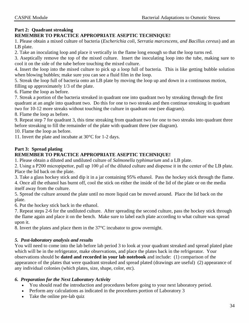
CASPiE Module Bacterial Adaptations to Osmotic Stress
34
Part 2: Quadrant streaking
REMEMBER TO PRACTICE APPROPRIATE ASEPTIC TECHNIQUE!
1. Please obtain a mixed culture of bacteria (Escherichia coli, Serratia marcescens, and Bacillus cereus) and an
LB plate.
2. Take an inoculating loop and place it vertically in the flame long enough so that the loop turns red.
3. Aseptically remove the top of the mixed culture. Insert the inoculating loop into the tube, making sure to
cool it on the side of the tube before touching the mixed culture.
4. Insert the loop into the mixed culture to pick up a loop full of bacteria. This is like getting bubble solution
when blowing bubbles; make sure you can see a fluid film in the loop.
5. Streak the loop full of bacteria onto an LB plate by moving the loop up and down in a continuous motion,
filling up approximately 1/3 of the plate.
6. Flame the loop as before.
7. Streak a portion of the bacteria streaked in quadrant one into quadrant two by streaking through the first
quadrant at an angle into quadrant two. Do this for one to two streaks and then continue streaking in quadrant
two for 10-12 more streaks without touching the culture in quadrant one (see diagram).
8. Flame the loop as before.
9. Repeat step 7 for quadrant 3, this time streaking from quadrant two for one to two streaks into quadrant three
before streaking to fill the remainder of the plate with quadrant three (see diagram).
10. Flame the loop as before.
11. Invert the plate and incubate at 30°C for 1-2 days.
Part 3: Spread plating
REMEMBER TO PRACTICE APPROPRIATE ASEPTIC TECHNIQUE!
1. Please obtain a diluted and undiluted culture of Salmonella typhimurium and a LB plate.
2. Using a P200 micropipettor, pull up 100 μl of the diluted culture and dispense it in the center of the LB plate.
Place the lid back on the plate.
3. Take a glass hockey stick and dip it in a jar containing 95% ethanol. Pass the hockey stick through the flame.
4. Once all the ethanol has burnt off, cool the stick on either the inside of the lid of the plate or on the media
itself away from the culture.
5. Spread the culture around the plate until no more liquid can be moved around. Place the lid back on the
plate.
6. Put the hockey stick back in the ethanol.
7. Repeat steps 2-6 for the undiluted culture. After spreading the second culture, pass the hockey stick through
the flame again and place it on the bench. Make sure to label each plate according to what culture was spread
upon it.
8. Invert the plates and place them in the 37°C incubator to grow overnight.
5. Post-laboratory analysis and results
You will need to come into the lab before lab period 3 to look at your quadrant streaked and spread plated plate
which will be in the refrigerator, make observations, and place the plates back in the refrigerator. Your
observations should be dated and recorded in your lab notebook and include: (1) comparison of the
appearance of the plates that were quadrant streaked and spread plated (drawings are useful) (2) appearance of
any individual colonies (which plates, size, shape, color, etc).
6. Preparation for the Next Laboratory Activity
You should read the introduction and procedures before going to your next laboratory period.
Perform any calculations as indicated in the procedures portion of Laboratory 3
Take the online pre-lab quiz

CASPiE Module Bacterial Adaptations to Osmotic Stress
35
IV. Laboratory Period 3 – Importance of mutants in scientific research, auxotrophy the
Salmonella typhimurium osmotic stress response, and light microscopy
Objectives
At the end of this laboratory period the students will be able to:
1. Understand the universal structure of DNA
2. Describe some of the differences between prokaryotic and eukaryotic genomes
3. Describe the different types of DNA mutations and the impact on the encoded proteins
4. Describe the requirements for bacterial growth and the phases of growth in culture
5. Understand and appreciate the usefulness of auxotroph mutants
6. Understand the bacterial osmotic stress response
7. Predict bacterial growth and survival for different auxotroph mutants and different living conditions
8. Understand function and regulation of the proline transporter ProP
9. Toothpick streak bacterial colonies onto a plate
10. Use a compound light microscope and adjust Kohler illumination
11. View osmotically-stressed cells with a compound light microscope
1. Introduction
Basic bacterial genetics
Humans, cows, tomato plants, grasshoppers, and bacteria are all extremely different organisms on so many
levels, but they do share at least one thing in common. They all store the genetic information they need to
flourish and survive in the form of Deoxyribonucleic acid (DNA), and they all share the same general
mechanism of replicating, decoding, and translating the message contained in DNA to make proteins. DNA is a
polymer of nucleotides organized on two strands that are bonded together to form the famous double helix
shape. Each nucleotide contains a deoxyribose sugar-phosphate backbone and a nitrogenous base that is an
adenine, a thymine, a cytosine, or a guanine (A, T, C, and G, respectively) (Figure 1).
Figure 1. The chemical structure of the two classes of nucleotide bases in DNA and/or RNA. Public domain image from:
http://commons.wikimedia.org/wiki/File:Nucleotides.png

CASPiE Module Bacterial Adaptations to Osmotic Stress
36
The sugar-phosphate portions of each nucleotide covalently bond with each other to form the backbone of the
strand while the nitrogenous bases hydrogen-bond with each other to form ladder rungs between the sugar
backbones and give rise to the double helix shape (Figure 2). Based on the positions and molecular content of
the nitrogenous bases, each of the 4 nucleotides will only hydrogen bond successfully with one other nucleotide
(A-T and G-C) forming basepairs. The order of the basepairs determines which proteins are synthesized to
carry out the everyday functions of the cell.
Figure 2. The basic organization of the DNA double helix. The sugar
phosphate backbone of the double helix is represented as a solid ribbon
while the base pairs form the ladder rungs that connect the two backbones. Image courtesy: National Human Genome Research Institute.
In order to contain enough information to code for every
protein the cell needs, the DNA sequence must be very long. The entire diploid human genome contains
6,000,000,000 base pairs (Walker and Rapley, Molecular Biology and Biotechnology) which would be ~2 meters long if it were
stretched out. Compare this to the Salmonella 4,857,432 base pair long genome which would be 1.6mm long
when stretched out. The diameter of cells is much smaller than that with eukaryotic cells averaging 10-30
microns and prokaryotic cells averaging only 1-10 microns. Clearly, DNA cannot be stored in its linear form!
In eukaryotic cells, for example, linear pieces of DNA are packaged with proteins to form chromatin stored in
the nucleus. Each piece of linear DNA is a chromosome and encodes for a distinct set of protein. Human cells
each have 23 pairs of chromosomes (Figure 3left). Bacteria, a prokaryotic unicellular organism, are different
from the four other organisms listed above in that they only contain one tightly-wound chromosome, and it is
circular instead of linear (Figure 3right). Figure 3. Human and Bacterial Chromosomes. Left.
Humans have 22 pairs of linear chromosomes and a
pair of sex chromosomes. Image courtesy: National
Human Genome Research Institute.
Right. Bacteria have a single circular chromosome
that encodes all of its proteins. This image shows an
E. coli chromosome labeled with radioactive thymine
replicating itself with the parent chromosome being
the large circle at the bottom. (image from: http://www.ncbi.nlm.nih.gov/bookshelf/br.fcgi?book=mmed&part
=A446&rendertype=figure&id=A450)
Human chromosomes E. coli chromosome

CASPiE Module Bacterial Adaptations to Osmotic Stress
37
When a bacterial cell grows and divides, it does so asexually by binary fission so that each bacterial cell gives
rise to two daughter cells (Figure 4). In order to do this, the DNA of the cell must be replicated so that each
daughter cell can have its own chromosome (See Figure 3right, above). To begin replicating the DNA, the
double helix of DNA is broken apart and enzyme machinery works to make an exact copy of the entire
chromosome. The process of DNA replication is highly monitored by the cell to ensure as much as possible
that no mistakes are made in the important DNA sequence. However, nobody is perfect, and there will always
be some mistakes made, resulting in mutations to the DNA sequence (more on this later).
Figure 4. Bacterial DNA replication and binary fission. Cytokinesis is the process of splitting the single
cell into two daughter cells. Image adapted from: http://commons.wikimedia.org/wiki/File:Three_cell_growth_types.png
Once the DNA has been replicated and the cell has divided, each new daughter cell has all the necessary
information to make proteins organized into units called genes. To make proteins, the DNA sequence serving
as the recipe for the protein is converted to ribonucleic acid (RNA), a single-stranded polymer of nucleotides
that is similar to DNA, in a process known as transcription (Figure 5). The mRNA (messenger RNA)
sequence produced is complementary to the DNA sequence and contains the order of the trios of nucleotides
(codons) that encode for specific amino acids, the molecules that are linked together to comprise proteins. Figure 5. Basic schematic of the process of
transcription. The DNA double helix is opened in
small sections and enzymatic machinery synthesizes
mRNA from the DNA template. Image courtesy: National
Human Genome Research Institute.

CASPiE Module Bacterial Adaptations to Osmotic Stress
38
Each codon is recognized by the anticodons of different RNA molecules known as tRNAs (transfer RNAs).
Each tRNA contains an amino acid that it adds to the growing chain of amino acids to produce a protein. This
process of interpreting the sequence coded for by the DNA and transcribed into the RNA is known as
translation (Figure 6). Once a protein is translated and further processed, it is ready to function and allow the
cell to survive.
Figure 6. Basic schematic of the process of translation. Using
mRNA, and the codons it specifies, as a guide, enzyme
complexes construct amino acid chains that give rise to proteins.
Translation is depicted here in a eukaryotic cell with a nucleus. Image courtesy: National Human Genome Research Institute.
A. Introduction for Part 1 of the procedures:
Importance of mutants to scientific research: Auxotrophy
Different species of bacteria are able to grow in a wide variety of environments, some that supply an abundance
of nutrients and growth factors, such as an overflowing garbage can or the leftover pizza you forgot to put into
the refrigerator last night, and others that provide very little for the bacteria to grow, such as a sterilized lab
bench or an iceberg at the North Pole. Regardless of the species and its location, all bacteria have some
standard growth requirements that must be met in order for them to grow and survive. Two of the most basic
growth requirements for any bacterial species are an energy source and a nutrient source.
The most basic growth requirement that must be supplied for any organism, bacteria or otherwise, to grow is an
energy source. Without an energy source to break down into smaller components, or catabolize, a bacterium
cannot produce enough ATP to maintain its normal every day cell functions, and therefore it will not be able to
grow. The type of energy source that can be used depends entirely on the species of bacteria. Many bacteria
can use organic molecules (carbon-containing molecules) such as sugars as an energy source. Photosynthetic
organisms can use sunlight as an energy source. Other organisms can oxidize inorganic molecules and use
them as an energy source. Some species have a wide range of different energy sources while others are much
more selective. An organism can only utilize a particular compound as an energy source if it contains the
genetic information that codes for the enzymes needed to catabolize a particular energy source.
In addition to an energy source, bacteria require a variety of nutrients. These nutrients are usually organic
compounds that function as both an energy source and as building blocks for more complex, essential cellular
components like proteins, nucleotides, and fatty acids. Some bacterial species require very few nutrients in the
external environment while other species are more fastidious and cannot grow unless they are supplied with
extra nutrients. Those organisms capable of growing without supplied nutrients do so because their genome
encodes for the enzymes needed to synthesize the nutrients on their own. Fastidious organisms, on the other
hand, do not contain these enzymes and therefore can only grow in an environment where these essential
compounds are provided. An organism that is not able to synthesize a particular organic compound required for
its growth is known as an auxotroph for that particular compound.

CASPiE Module Bacterial Adaptations to Osmotic Stress
39
Auxotrophic mutant bacterial strains are useful research tools as they allow scientists to control their
environment and growth. To gain experience in visualizing and identifying an auxotrophic phenotype, we will
plate three different types of Salmonella auxotrophs onto minimal media M63 plates supplemented with
nutrients that will support growth. Below are the bacterial strains we will be using today.
Table 1. Bacterial strains for auxotrophy experiment
Strain Genotype Phenotype
TL-1 Wild type No auxotrophic phenotype
TL-117 proA-, proB
- Proline auxotroph
TL-602 supD- Histidine auxotroph
TL-4127 pyrB- Uracil auxotroph
+ denotes full function of the gene
– denotes no function of the gene
B. Introduction for Part 2 of the Procedures:
Osmotic stress response and proline uptake systems
A high osmotic stress environment can be detrimental to the growth of bacteria. When bacteria find themselves
in a high osmotic stress environment, they are in an environment where the solute concentration is higher
outside of the cell than inside the cell. As we learned and observed in lab period 1, a higher external solute
concentration means a lower water activity outside of the cell, resulting in an efflux of water from the cell (see
the middle image in Figure 7 below. This movement of water outside the cell will result in shrinkage of the
bacterial cell which will prevent bacterial growth and will lead to death unless a corrective action is taken. S.
typhimurium has two mechanisms it uses to prevent death by cell shrinkage in a high osmotic stress
environment. One is the uptake of potassium glutamate (K+-glutamate) and the other is the uptake or synthesis
of compatible solutes.
Figure 7. Universal response of cells to high external osmolality.
In response to high osmotic stress conditions, bacteria can actively transport in potassium ions (K+). In order to
balance such a high import of positively charged K+, the cells correspondingly increase synthesis of the
negatively charged amino acid glutamate. The accumulation of K+-glutamate will increase the solute
concentration inside the cell. After enough transport, this will result in a lower water activity inside the cell
than outside. Water will then flow back into the cell, restoring the cell to its original size and allowing growth
to continue in the high osmotic stress environment. This mechanism works well up to a certain point, however
under extremely high osmotic stress conditions, the amount of K+-glutamate that must be accumulated is so
high that the concentration of the charged components inside the cell actually becomes inhibitory to protein

CASPiE Module Bacterial Adaptations to Osmotic Stress
40
function and will negatively impact cell growth. In order to survive growth in this type of an environment,
another method must be used. The chosen method by S. typhimurium is the uptake of compatible solutes.
Compatible solutes are small, uncharged compounds that can either be transported into the cell or synthesized
by the cell and accumulated to high concentrations without negatively impacting every day cellular function.
They can be accumulated (or excluded) because they are not freely permeable across the cell membrane. Two
of the main compatible solutes uptaken by S. typhimurium are proline and glycine betaine, and the bacterium
has three transport systems for taking up one or both of these compatible solutes in response to osmotic stress
conditions. These are the ProP, the ProU, and the BetP transport systems (Figure 8). The ProP and ProU
systems transport both glycine betaine and proline in response to osmotic stress while the BetP system only
transports glycine betaine.
Figure 8. Players in the hyperosmotic response in S.
typhimurium. A model cell is depicted showing the uptake of
K+ and compatible solutes into the cell in response to a
hyperosmotic environment.
In order to illustrate how these uptake systems affect the growth of S. typhimurium under osmotic stress
conditions, we will use strains that contain different combinations of mutations in the transport systems and
subject them to osmotic stress in the presence or absence of proline or glycine betaine. The strains we will use
are summarized in Table 2.
Table 2. Bacterial strains for osmotic stress experiment
Strain Genotype Phenotype
TL-1 proP+, proU
+, betP
+ Wild type (all transport intact)
TL-197 proP-, proU
+, betP
+ No ProP transport
TL-201 proP-, proU
-, betP
+ No ProP or ProU transport
TL-4088 proP-, proU
-, betP
- No transport systems
+ denotes full function of the gene
– denotes no function of the gene
C. Introduction for Part 3 of the Procedures:
Antagonism of ProP proline uptake by glycine betaine
ProP is a large 500 amino-acid containing protein that is able to uptake proline and glycine betaine in response
to osmotic stress. ProP acts as a H+-symporter that transports in proline or glycine betaine along with a proton.
An antagonistic relationship exists between the two osmoprotectants. When there is a higher concentration of
glycine betaine in the external media than proline, the uptake of proline by ProP is inhibited. If the proline
concentration is increased to be equal with glycine betaine, proline will be transported again.

CASPiE Module Bacterial Adaptations to Osmotic Stress
41
Because proline is not only an osmoprotectant but is also a component of all cellular proteins, impairing proline
uptake can have negative consequences for the survival of certain bacteria. Therefore, in addition to the ability
to acquire proline from the external environment, cells have means to synthesize this important amino acid
themselves. Proline can be synthesized from the precursor amino acid glutamate in four steps, three of which
require the activity of specific enzymes, ProA, ProB, and ProC (Figure 9).
Figure 9. Outline of the intracellular synthesis of proline. The four steps in proline synthesis
from glutamate. The enzymes catalyzing the reactions between intermediates (in boxes) are
shown between boxes along arrows. The genes encoding these enzymes are shown to the left.
The third reaction from glutamate semialdehyde to 1-pyrroline 5-caboxylate occurs
spontaneously.
In addition to ProP, S. typhimurium can obtain proline by taking it up through the standard proline uptake
protein PutP (a proline/Na+ symporter) and the osmotically induced ProU system (Figure 10).
Figure 10. Summary of the sources of proline in S.
typhimurium. Proline can be taken up from the environment
via secondary active transport (ProP and PutP) or can be
actively pumped in (ProU). Proline can be synthesized in the
cell from glutamate.
If these transport mechanisms are significantly compromised for some reason, S. typhimurium can synthesize
proline, as described above. In a proline auxotroph unable to synthesize its own proline (mutations in proA,
proB, and proC genes) that also lacks the ProU and PutP proline transport systems, proline must be taken up
from the environment via ProP for the bacterium to survive. If an antagonistic concentration of glycine betaine
exists in the external media, this bacterial strain will not be able to survive as it cannot uptake enough proline.
We will be taking advantage of this situation to better understand the function of the ProP transporter. Table 3
contains the genotypes and phenotypes of the strains we will be using today to illustrate the antagonistic
relationship between proline and glycine betaine for transport by ProP.

CASPiE Module Bacterial Adaptations to Osmotic Stress
42
Table 3. Bacterial strains for glycine betaine antagonism experiment
Strain Genotype Phenotype
TL-1 Wild type Wild type
TL-117 proA-, proB
-, proP
+, proU
+, putP
+ Proline auxotroph
TL-193 proA-, proB
-, proP
+, proU
-, putP
- Proline auxotroph, no PutP or
ProU transport + denotes full function of the gene
– denotes no function of the gene
D. Introduction for Part 5 of the Procedures: Light microscopy Written in consultation with Guide to Microscopy, Becker WM, Kleinsmith LJ, and Hardin J (2003)
The diameters of bacteria can range from 1 micron to 5 microns across, a size that is smaller than can be
detected with the naked eye (A useful image can be found in Molecular Biology of the Cell, 5th edition,
Alberts, Johnson, Lewis, Raff, Robers, and Walter). Therefore, we need the assistance of compound light
microscopes to magnify these organisms to visualize them.
Basic principles of light microscopy
There are three items that are necessary in light microscopy: the specimen to be observed, a source of
illumination, and a glass lens, or series of lenses, to focus and magnify the image of the specimen. A useful
image depicting the basic path that light takes in light microscopy using a compound microscope (more than
one lens) can be found in Molecular Biology of the Cell, 5th edition, Alberts, Johnson, Lewis, Raff, Robers,
and Walter.
Light
The type of light used in light microscopy is visible light. Visible light is a form of electromagnetic radiation
that consists of particles and waves of energy. The wavelength (λ) is measured in meters (m) with the higher
the frequency (cycles per second) of the waves the shorter the wavelength (Figure 11). These different
wavelengths comprise a spectrum of electromagnetic radiation according to the wavelength (Figure 12).
Figure 11. Example of a cyclic wave. The wavelength (λ) is the physical
distance, in meters, between two peaks (or troughs) marking one period.
Visible light includes electromagnetic radiation with wavelengths in the range of 400 to 700 nanometers (nm;
10-9
meters). As light travels in the environment it interacts with different objects in different manners that
depend on the properties of the objects and the wavelength of the light. When light encounters an object it can
be absorbed (be taken up), transmitted (pass through unchanged), refracted (pass through, but the path is
changed), diffracted (bend around the object) or reflected (bounce off).

CASPiE Module Bacterial Adaptations to Osmotic Stress
43
Figure 12. The electromagnetic spectrum.
The spectrum is divided and named
according to wavelength. Comment objects
and structures are illustrated to provide a
concept of scale for the wavelengths. The
visible range for humans is a small fraction
of the entire spectrum. Image from:
http://mynasadata.larc.nasa.gov/images/EM_Spectrum
3-new.jpg
In order for us to see our specimens using a microscope, the light we use to illuminate it must interact with the
specimen. As the waves of light travel through the specimen and the glass lenses of the microscope their paths
change. Depending on the properties of the specimen and the lenses and the wavelengths of the light, the light
will interact with them differently and their paths will be altered differently. The interference patterns between
the different waves of light are what form the image we observe. Waves of light that are in phase with one
another (peaks and troughs are aligned) will add and an increase in brightness that will be observed in that
region. Waves of light that are out of phase with one another will result in less brightness (A useful illustration
can be found in Molecular Biology of the Cell, 5th edition, Alberts, Johnson, Lewis, Raff, Robers, and Walter).
Basic Function of Lenses in Light Microscopy
As mentioned above, in light microscopy glass lenses are used to focus light and magnify the image of the
specimen. Figure 13 illustrates how a biconvex lens is used to gather light and focus it to a single point (focal
point) by refraction. The distance of the focal point relative to the middle of the lens is known as the focal
length and is a unique property for each lens.
Figure 13. Illustration of the focusing of light by a biconvex glass lens. The focal point
(F) is shown where the refracted light waves are focused. The focal length (f) is the
distance between the midline of the lens and the focal point. Image adapted from:
http://commons.wikimedia.org/wiki/File:Focal-length.png
Magnification of a specimen is achieved by this basic interaction between light and a lens. Usually a small
object in a larger field of view will only activate a small fraction of the retina of the observer and will appear
small. By gathering and focusing only the light from a small object and feeding it to the eye of the observer, the
fraction of the retina activated by that light is increased and the image appears larger. With one lens, however,
the maximum magnification that can be achieved is only about an 8-10 fold enlargement (also stated as 8-10X).

CASPiE Module Bacterial Adaptations to Osmotic Stress
44
Compound microscopes multiply the magnification by using 2 or more lenses in series with one another (one
after another in a single path). This can increase the magnification of objects viewed in air to greater than 1,000
times their original size!
Magnification is critical for the examination of small structures, however another important parameter that is
affected by the property of the lenses used in the microscope is the resolution. In microscopy, resolution is the
minimum distance between two objects where they can still be viewed as two distinct objects with a
microscope. The resolution is important in determining the level of detail and subtlety that can be observed in
the magnified specimen. It would not matter if the series of lenses used results in 10,000 fold magnification if
the maximum resolution was achieved at 1,000X! The best theoretical resolution that can be achieved with
light microscopy is 200-300 nm, but in practice reliable resolution is limited by the smallest wavelength of light
that can be seen by the human eye (400 nm).
Brightfield microscopy
We will be using compound microscopes in lab this week and next. An example of a typical compound
microscope is shown in Figure 14. Most of the important features are denoted and we will show you others and
demonstrate usage in the lab.
Figure 14. A typical compound microscope with
important features shown. Not elaborated on is that
the coarse and fine focusing knobs are used to move
the stage up and down with respect to the objective
lenses. Image from: http://commons.wikimedia.org/wiki/File:Labelledmicroscope.gif
Compound microscopes can be optimized
for viewing different types of specimens (living vs. fixed cells). We will be using a technique known as
brightfield microscopy. This technique relies on the tissue specimen having color or some property that alters
how light passes through it to create the interference patterns described previously to create the image.

CASPiE Module Bacterial Adaptations to Osmotic Stress
45
An important component of the microscope is the condenser (see Figure 14). The condenser of the microscope
is a lens that sits between the illumination source and the specimen mounted on the stage. The basic function of
the condenser is to control the focus of the cone of light from the illuminator onto the specimen. When adjusted
properly (see procedures), the condenser will focus light only onto the part of the specimen opposite to the
objective lens. This maximizes the amount of light that the objective lens collects from the specimen it is
aligned with and will increase the resolution and quality of the image. This technique was developed by August
Köhler in 1893 and is known as Köhler Illumination. You will practice this technique today in lab.
Magnification: sense of scale
In addition to their different physiology and preferred living environments, bacteria can vary in their size and
shape (Figure 15). They range in size from 0.2 – 2 microns (µm) (10-6
meters) across for spherical bacteria and
1-10 µm long for non-spherical bacteria. We can measure the sizes of these cells using our compound
microscopes. We have two magnifying lenses in series in our microscopes: 1. The objective lenses (4X, 10X,
40X) and 2. The ocular lenses (10X). As such, the total magnification is not simply the magnification of the
objective lenses, but it is the product of the objective that you are using and the ocular lens magnification. For
example, when you view a specimen on your slide with the 4X objective lens, the total magnification of the
image as seen through the eyepieces is 40X. Since the ocular magnification is fixed, we will often simply state
the objective magnification and the addition 10X from the oculars is implied.
Figure 15. Examples of bacteria as visualized with a compound microscope to illustrate the differences in size and shape.. On the left is Gram
stained S. typhimurium. On the right is Gram stained Staphylococcus aureus. Imagesfrom: ASM microbelibrary
IMPORTANT MICROSCOPE USAGE REQUIREMENTS! 1. Always carry the microscope with two hands! One hand should be placed under the base and the other hand
holds the arm of the microscope.
2. Always start viewing a slide with the 4X scanning objective lens to find your specimen.
3. NEVER use the coarse adjustment knob with objective lenses greater than 4X!
4. If you are using the 100X oil immersion objective lens, only use the oil we provide.
5. Only lens paper can be used to clean the objectives.
6. When you are finished using the microscope for the day, remove slide from the stage, put the 4X objective into
place, turn off the illumination, unplug the microscope, wrap the cord around the arm, and cover the scope with its
plastic cover (if available).

CASPiE Module Bacterial Adaptations to Osmotic Stress
46
2. Pre-laboratory activities
Come in before lab next week and observe your aseptic transfer tubes and M63 plates that you poured last
week. They are in a refrigerator at the back of the lab. When looking at the plates you can briefly take the lid
off of them, but be sure to put the lid inside-up on the bench if you set it down.
Read the introduction and the procedures for Laboratory Period 3 of the lab manual. Where indicated in bold, in
your lab notebook work out calculations for any solutions to be made or diluted as well as answer any questions
posed. Before the lab period, log onto Blackboard and take the pre-lab quiz for this week.
3. Materials
Auxotrophy:
Equipment and materials
●P-200 micropipettor
●P-200 micropipettor tips (autoclaved)
●Hockey stick
●Jar of 95% ethanol
●Bunsen burner
●Striker
●Sharpie
●Sterile toothpicks ●Pipette tip waste containers
●37o incubator
Reagents
● M63 glucose plates
●100 mM proline sterile stock solution
●100 mM histidine sterile stock solution
●20 mM uracil sterile stock solution
●TL-1 culture plate
●TL-117 culture plate
●TL-602 culture plate
●TL-4127 culture plate
High osmolarity stimulation:
Equipment and materials
●P-200 micropipettor
●P-200 micropipettor tips (autoclaved)
●Hockey stick
●Jar of ethanol
●Bunsen burner
●Striker
●Sharpie
●Sterile toothpicks ●Pipette tip waste containers
●37o incubator

CASPiE Module Bacterial Adaptations to Osmotic Stress
47
Reagents
●M63 glucose plate
●M63 glucose plate + 0.65 M NaCl
●10 mM proline sterile stock solution
●500 mM glycine betaine sterile stock solution
●TL-1 culture plate
●TL-197 culture plate
●TL-201 culture plate
●TL-4088 culture plate
Antagonism by Glycine Betaine:
Equipment and materials
●M63 glucose + 0.3 M NaCl plates
● M63 glucose + 0.3 M NaCl + 0.1 mM proline plates
● M63 glucose + 0.3 M NaCl + 0.1 mM proline plates
●P-200 micropipettor tips (autoclaved)
●P-200 micropipettor
●Hockey sticks
●Jar of ethanol
●Bunsen burner
●Sparker
●37o incubator
●Sharpies
●Pipette tip waste containers
●Sterile toothpicks
Reagents
●TL-1 culture plate (wt)
●TL-117 culture plate (proline auxotroph)
●TL – 193 culture plate (proline auxotroph, proP+, putP-, proU-)
●500 mM sterile glycine betaine stock solution
Microscopy:
Equipment and materials
●compound microscope
●immersion oil
●lens paper
●index card w/ punch hole
●blank slides ●coverslip
●toothpicks
●plastic transfer pipettes ●’e’ slide
●Microcentrifuge tubes
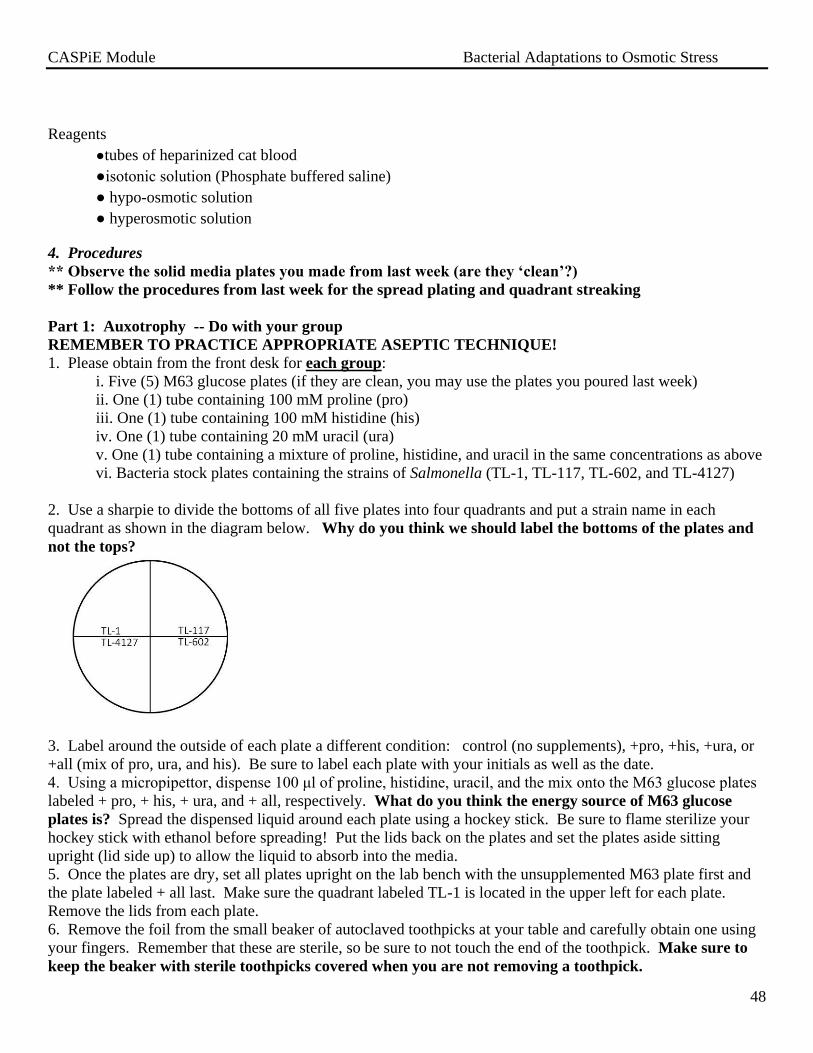
CASPiE Module Bacterial Adaptations to Osmotic Stress
48
Reagents
●tubes of heparinized cat blood
●isotonic solution (Phosphate buffered saline)
● hypo-osmotic solution
● hyperosmotic solution
4. Procedures
** Observe the solid media plates you made from last week (are they ‘clean’?)
** Follow the procedures from last week for the spread plating and quadrant streaking
Part 1: Auxotrophy -- Do with your group
REMEMBER TO PRACTICE APPROPRIATE ASEPTIC TECHNIQUE!
1. Please obtain from the front desk for each group:
i. Five (5) M63 glucose plates (if they are clean, you may use the plates you poured last week)
ii. One (1) tube containing 100 mM proline (pro)
iii. One (1) tube containing 100 mM histidine (his)
iv. One (1) tube containing 20 mM uracil (ura)
v. One (1) tube containing a mixture of proline, histidine, and uracil in the same concentrations as above
vi. Bacteria stock plates containing the strains of Salmonella (TL-1, TL-117, TL-602, and TL-4127)
2. Use a sharpie to divide the bottoms of all five plates into four quadrants and put a strain name in each
quadrant as shown in the diagram below. Why do you think we should label the bottoms of the plates and
not the tops?
3. Label around the outside of each plate a different condition: control (no supplements), +pro, +his, +ura, or
+all (mix of pro, ura, and his). Be sure to label each plate with your initials as well as the date.
4. Using a micropipettor, dispense 100 μl of proline, histidine, uracil, and the mix onto the M63 glucose plates
labeled + pro, + his, + ura, and + all, respectively. What do you think the energy source of M63 glucose
plates is? Spread the dispensed liquid around each plate using a hockey stick. Be sure to flame sterilize your
hockey stick with ethanol before spreading! Put the lids back on the plates and set the plates aside sitting
upright (lid side up) to allow the liquid to absorb into the media.
5. Once the plates are dry, set all plates upright on the lab bench with the unsupplemented M63 plate first and
the plate labeled + all last. Make sure the quadrant labeled TL-1 is located in the upper left for each plate.
Remove the lids from each plate.
6. Remove the foil from the small beaker of autoclaved toothpicks at your table and carefully obtain one using
your fingers. Remember that these are sterile, so be sure to not touch the end of the toothpick. Make sure to
keep the beaker with sterile toothpicks covered when you are not removing a toothpick.
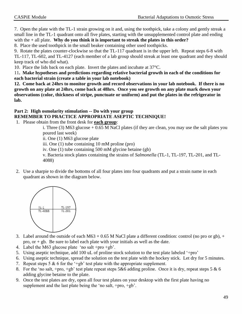
CASPiE Module Bacterial Adaptations to Osmotic Stress
49
7. Open the plate with the TL-1 strain growing on it and, using the toothpick, take a colony and gently streak a
small line in the TL-1 quadrant onto all five plates, starting with the unsupplemented control plate and ending
with the + all plate. Why do you think it is important to streak the plates in this order?
8. Place the used toothpick in the small beaker containing other used toothpicks.
9. Rotate the plates counter-clockwise so that the TL-117 quadrant is in the upper left. Repeat steps 6-8 with
TL-117, TL-602, and TL-4127 (each member of a lab group should streak at least one quadrant and they should
keep track of who did what).
10. Place the lids back on each plate. Invert the plates and incubate at 37°C.
11. Make hypotheses and predictions regarding relative bacterial growth in each of the conditions for
each bacterial strain (create a table in your lab notebook)
12. Come back at 24hrs to monitor growth and record observations in your lab notebook. If there is no
growth on any plate at 24hrs, come back at 48hrs. Once you see growth on any plate mark down your
observations (color, thickness of stripe, punctuate or uniform) and put the plates in the refrigerator in
lab.
Part 2: High osmolarity stimulation -- Do with your group
REMEMBER TO PRACTICE APPROPRIATE ASEPTIC TECHNIQUE!
1. Please obtain from the front desk for each group:
i. Three (3) M63 glucose + 0.65 M NaCl plates (if they are clean, you may use the salt plates you
poured last week)
ii. One (1) M63 glucose plate
iii. One (1) tube containing 10 mM proline (pro)
iv. One (1) tube containing 500 mM glycine betaine (gb)
v. Bacteria stock plates containing the strains of Salmonella (TL-1, TL-197, TL-201, and TL-
4088)
2. Use a sharpie to divide the bottoms of all four plates into four quadrants and put a strain name in each
quadrant as shown in the diagram below.
3. Label around the outside of each M63 + 0.65 M NaCl plate a different condition: control (no pro or gb), +
pro, or + gb. Be sure to label each plate with your initials as well as the date.
4. Label the M63 glucose plate ‘no salt +pro +gb’.
5. Using aseptic technique, add 100 uL of proline stock solution to the test plate labeled ‘+pro’
6. Using aseptic technique, spread the solution on the test plate with the hockey stick. Let dry for 5 minutes.
7. Repeat steps 5 & 6 for the ‘+gb’ test plate with the appropriate supplement.
8. For the ‘no salt, +pro, +gb’ test plate repeat steps 5&6 adding proline. Once it is dry, repeat steps 5 & 6
adding glycine betaine to the plate.
9. Once the test plates are dry, open all four test plates on your desktop with the first plate having no
supplement and the last plate being the ‘no salt, +pro, +gb’.
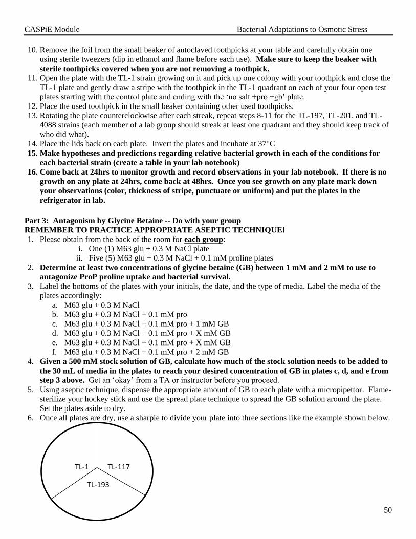
CASPiE Module Bacterial Adaptations to Osmotic Stress
50
10. Remove the foil from the small beaker of autoclaved toothpicks at your table and carefully obtain one
using sterile tweezers (dip in ethanol and flame before each use). Make sure to keep the beaker with
sterile toothpicks covered when you are not removing a toothpick.
11. Open the plate with the TL-1 strain growing on it and pick up one colony with your toothpick and close the
TL-1 plate and gently draw a stripe with the toothpick in the TL-1 quadrant on each of your four open test
plates starting with the control plate and ending with the ‘no salt +pro +gb’ plate.
12. Place the used toothpick in the small beaker containing other used toothpicks.
13. Rotating the plate counterclockwise after each streak, repeat steps 8-11 for the TL-197, TL-201, and TL-
4088 strains (each member of a lab group should streak at least one quadrant and they should keep track of
who did what).
14. Place the lids back on each plate. Invert the plates and incubate at 37°C
15. Make hypotheses and predictions regarding relative bacterial growth in each of the conditions for
each bacterial strain (create a table in your lab notebook)
16. Come back at 24hrs to monitor growth and record observations in your lab notebook. If there is no
growth on any plate at 24hrs, come back at 48hrs. Once you see growth on any plate mark down
your observations (color, thickness of stripe, punctuate or uniform) and put the plates in the
refrigerator in lab.
Part 3: Antagonism by Glycine Betaine -- Do with your group
REMEMBER TO PRACTICE APPROPRIATE ASEPTIC TECHNIQUE!
1. Please obtain from the back of the room for each group:
i. One (1) M63 glu + 0.3 M NaCl plate
ii. Five (5) M63 glu + 0.3 M NaCl + 0.1 mM proline plates
2. Determine at least two concentrations of glycine betaine (GB) between 1 mM and 2 mM to use to
antagonize ProP proline uptake and bacterial survival.
3. Label the bottoms of the plates with your initials, the date, and the type of media. Label the media of the
plates accordingly:
a. M63 glu + 0.3 M NaCl
b. M63 glu + 0.3 M NaCl + 0.1 mM pro
c. M63 glu + 0.3 M NaCl + 0.1 mM pro + 1 mM GB
d. M63 glu + 0.3 M NaCl + 0.1 mM pro + X mM GB
e. M63 glu + 0.3 M NaCl + 0.1 mM pro + X mM GB
f. M63 glu + 0.3 M NaCl + 0.1 mM pro + 2 mM GB
4. Given a 500 mM stock solution of GB, calculate how much of the stock solution needs to be added to
the 30 mL of media in the plates to reach your desired concentration of GB in plates c, d, and e from
step 3 above. Get an ‘okay’ from a TA or instructor before you proceed.
5. Using aseptic technique, dispense the appropriate amount of GB to each plate with a micropipettor. Flame-
sterilize your hockey stick and use the spread plate technique to spread the GB solution around the plate.
Set the plates aside to dry.
6. Once all plates are dry, use a sharpie to divide your plate into three sections like the example shown below.
TL-1 TL-117
TL-193

CASPiE Module Bacterial Adaptations to Osmotic Stress
51
7. Using a sterile toothpick, streak a colony from a plate of TL-1 bacteria to the labeled TL-1 section of the
M63 glucose + 0.3 M NaCl plate (plate a in step 3). You only need to make one solid streak. There is no
need to streak for isolated colonies at this point. Make sure to keep the beaker with sterile toothpicks
covered when you are not removing a toothpick.
8. Discard the toothpick and repeat with a different colony from the TL-1 plate for plates b-f in step 3.
9. Repeat steps 7 & 8 for colonies from a TL-117 plate and a TL-193 plate (each person from the group
should do a strain and keep track of who did what). When you are done, each plate should have three
streaks on it, one TL-1, one TL-117, and one TL-193 streak.
10. Incubate the plates at 37o C.
11. Make hypotheses and predictions in your lab notebook. Make a table with the different strains and
conditions and mark your predictions (no growth (-), some growth (+), moderate growth (++),
normal growth (+++))
12. Come back at 24hrs to monitor growth and record observations in your lab notebook. If there is no
growth on any plate at 24hrs, come back at 48hrs. Once you see growth on any plate mark down
your observations (color, thickness of stripe, punctuate or uniform) and put the plates in the
refrigerator in lab.
Part 4: Observing osmotic stress response in red blood cells – Set up for each group
1. Each group should obtain and label three (3) microcentrifuge tubes and label the first ‘iso’, the second
‘hypo’, and the third ‘hyper’.
2. Using a plastic transfer pipette, put four (4) drops of the appropriate solution into each microcentrifuge
tube using a different transfer pipette each time.
3. Wearing gloves, add two (2) drops of cat blood to each microcentrifuge tube, close the top, and flick it
to mix.
4. Put the cap back on the blood.
5. Write out your predictions in your lab notebook and note the time. We will look at these at the end
of part 5 of the lab.
Part 5: Introduction to light microscopy - Each student will work individually on this
Using a compound microscope –We will demo basic handling and operation of the microscope first
1. Each student should obtain a compound microscope from the front of the room and bring it back to your
seat, near an electrical outlet. Be sure to carry it with one hand under the base and one hand holding the
microscope arm.
2. Plug in the scope and turn on the illumination.
3. With the 4X, scanning objective in place and the stage lowered, place the ‘e’ slide on the microscope
stage
4. Using the spot of light from the illuminator as a reference, try to center the ‘e’ over the spot of light.
5. Using the coarse focus knob, bring the ‘e’ into view.
**At this point, you should adjust the eyepieces to your eye spacing so you can look with both eyes in a
relaxed manner. This takes practice, but is worth the effort now and will reduce eyestrain!
6. Using the fine focus knob, bring the ‘e’ into focus.
7. Move the stage to the left and to the right. Compare the direction of movement of the image to the
direction of movement of the stage. What is the basis for the relationship between the two?
(Answer this in your lab notebook)
8. Without moving the focus, switch to the 10X objective by carefully rotating the nosepiece (turret).
9. Using the fine focus knob, bring the image back into focus. DO NOT USE THE COARSE FOCUS!
10. Repeat steps 8 & 9 for the 40X objective.

CASPiE Module Bacterial Adaptations to Osmotic Stress
52
Enhancing resolution and contrast:: Setting up Köhler Illumination
1. Keep the ‘e’ slide on the microscope stage and switch back to the 4X objective.
2. Decrease the illumination level by either controlling the diaphragm of the light source or by placing an
index card with a punch hole on top of the light source in its center. You will see the spot of light
through either the diaphragm or the punch hole.
3. Close down the light through the condenser by using either the slider on the condenser or by rotating the
ribbed ring.
4. Slowly move the condenser (either up or down) until you the edges of the spot of light become crisp.
5. Open the light through the condenser all the way and then decrease it until the illumination is just dim.
6. Remove the index card from over the light source/open the diaphragm and you are all set!
**You have now adjusted your compound microscope for Köhler Illumination and will get the best
contrast and resolution of your specimens. Ideally, you should make these adjustments whenever you
switch objectives.
Observing anatomical response of cells to osmotic stress – Each person should do this.
1. Note the time that has passed since you set up your red blood cells.
2. Take three (3) clean glass slides, label each with your initials, the date, and the osmotic conditions
(hypo, iso, or hyper)
3. With a transfer pipette place a drop of your cell solution on the appropriate slide.
4. Carefully place a glass cover slip over the drop by slowly lowering the cover slip onto the drop at an
angle to minimize air bubbles (we can show you this)
5. Using the appropriate magnification, find some cells, record observations and draw some cells in
your lab notebook.
6. Repeat this for all osmotic conditions, using a different transfer pipette each time.
7. Compare the results to your predictions and draw conclusions.
8. Remove your last slide from the bench and throw your slides away in the glass waste. 9. Put the 4X objective into place, turn off the illumination, unplug the microscope, wrap the cord around the
arm, and cover the scope with its plastic cover (if available).
CLEAN UP YOUR BENCH AREA BEFORE LEAVING LAB!!!!
5. Post-laboratory analysis and results
You will need to come into the lab as indicated at the end of the procedures above to take your plates from the
plating techniques, auxotrophy, osmotic stress, and glycine betaine antagonism experiments out of the 37
degree incubator. Make observations and place the plates in the refrigerator in G131. Your observations
should be dated and recorded in your lab notebook and include: (1) comparison of the degree of bacterial
growth in each of your quadrants for each condition (2) comparison of your observations to your predictions
made at the end of the lab today.
6. Preparation for the Next Laboratory Activity
You should read the introduction and procedures before going to your next laboratory period.
Perform any calculations and/or answer questions as indicated in bold in text of the Laboratory 4 manual
Take the online pre-lab quiz

CASPiE Module Bacterial Adaptations to Osmotic Stress
53
V. Laboratory Period 4 – Use of spectrophotometry to measure bacterial growth rates,
streaking to a pure culture, and mutagenesis
Objectives
At the end of this laboratory period the students will be able to:
1. Describe the principles used in basic spectrophotometry
2. Describe how transmittance and absorbance are related in concept and calculation
3. Use a spectrophotometer to measure the maximum absorbance of a substance in solution
4. Use spectrophotometry to measure bacterial growth rates in liquid culture
5. Understand the types of mutations and their results on the genome
6. Understand the impact that mutations have on proteins and the function of cells
7. Describe various types of mutagenesis
8. Perform quadrant streaking to obtain a pure bacterial culture from a mixed culture plate
1. Introduction
A .Introduction for Parts 1 and 2 of the procedures
Utility of the spectrophotometer to quantify levels of substances in solution:: Review of light
Light is a form of electromagnetic radiation that consists of particles and waves of energy. The wavelength (λ)
is measured in meters (m) with the higher the frequency (cycles per second) of the waves the shorter the
wavelength (Figure 1). These different wavelengths comprise a spectrum of electromagnetic radiation
according to the wavelength (Figure 2).
Figure 1. Example of a cyclic wave. The wavelength (λ) is the physical distance,
in meters, between two peaks (or troughs) marking one period.
Visible light includes electromagnetic radiation with wavelengths in the range of 400 to 700 nm. As light
travels in the environment it interacts with different objects in different manners that depend on the properties
of the objects and the wavelength of the light. When light encounters an object it can be absorbed (be taken
up), transmitted (pass through unchanged), refracted (pass through, but the path is changed), diffracted (bend
around the object) or reflected (bounce off).
Visible light contains all of the wavelengths simultaneously. How is it that we can perceive distinct colors in
the world around us? The perceived color of something is a function of which wavelengths of light are
absorbed or reflected by the object/substance. An object that is perceived as blue absorbs all wavelengths of
light except those in the blue portion of the visible light spectrum (490-450 nm). Those wavelengths reflect off
the object and are detected by the photoreceptors in our eyes that respond to that wavelength.
Utility of the spectrophotometer to quantify levels of substances in solution:: Principles of operation
Scientists can make use of the unique interactions that different wavelengths of light have with different
substances. For example, lenses in microscopes can be used to magnify and focus images by diffracting and
refracting light. Another useful application is using an instrument called a spectrophotometer to measure the
relative absorbance versus transmittance of light through a substance which can be used to get information
about the physical properties and abundance of a substance in solution. Spectrophotometers consist of an

CASPiE Module Bacterial Adaptations to Osmotic Stress
54
illumination source whereby the user can specify the wavelength of light that will be passed through an aqueous
solution by adjusting a filter that will allow light of particular wavelengths to be passed. The light will then
pass through a container, called a cuvette, containing a solution. Depending on the properties and abundance
of the constituents of the solution, such as proteins or cells, and the wavelength of light used, the light will be
absorbed or transmitted through the solution to varying degrees. The transmitted light is then detected by a
photodetector and the amount of this light is quantified.
Transmittance is a measure of the fraction of light that passes through a substance
and can be expressed as:
T = P / P0 (Equation 1)
where T is the transmittance, P0 is the radiant power of the incoming light and P is
the radiant power of the light that has passed through a substance.
Most of the light that is not transmitted through the substance is absorbed which can be expressed as:
A = log10 1/T = log10 P0/P (Equation 2)
By choosing a wavelength that will be maximally absorbed by the substance, the amount of light that is
absorbed by the sample is proportional to the concentration of the substance in solution, according to the Beer-
Lambert Law:
A = ebc (Equation 3)
where A is the absorbance (no units since A = log10 P0/P), e is the molar absorbtivity (L/ mole cm, a
fundamental property of the substance in question), b is the path length (cm, the width of the cuvette), and c is
the concentration of the substance in solution (mole/ L). The linear relationship between Absorbance and
concentration according to the Beer-Lambert Law is valid until high concentrations of the substance in question
as can be seen in Figure 3 (left) below.
Figure 3. Examples of a spectrophotometric standard curve. On the
right is an example of a standard curve constructed from measuring
the absorbance of solutions of known concentrations of Substance A.
Bacterial Growth
Often when we refer to bacterial growth, we are referring to the growth of a population of bacteria. Under
optimal conditions (growth in an enriched media at the optimal temperature for that species), a bacterial cell

CASPiE Module Bacterial Adaptations to Osmotic Stress
55
will divide once every 15-30 minutes. The two cells resulting from this division will then divide again in 15-30
minutes, resulting in exponential growth at a quick pace. It may seem as though a bacterial population could
grow at this rate indefinitely, however that is not the case. In most environments, the bacterial population will
grow at a rate that follows a predictable pattern known as the growth curve (Figure 4). The growth curve has
four phases: lag, log or exponential, stationary, and death.
Figure 4. Graph showing the names and stages of a typical
bacterial growth curve. Note the y-axis has is the log of the
number of bacteria giving rise to a linear trajectory in the
growth and death phases. Image from:
http://commons.wikimedia.org/wiki/File:Bacterial_
growth_en.svg
The first phase of the growth curve that occurs when bacterial culture is initially placed in a new environment is
the lag phase. During this phase, the cells are adjusting to their new environment. Depending on the nutrients
present in the environment, the cells may need to turn on expression of genes that code for proteins they will
need to catabolize carbon and energy sources. At this point, the cells are focusing all their energy and resources
on simply surviving and not on dividing. As a result, there is no growth of the bacterial population during the
lag phase. Once the cells are accustomed to their new environment, they will begin to divide. While this phase
of cell division will start out slowly, it will quickly increase to reach an exponential rate. This is known as the
log or exponential phase of growth. This is the phase of optimal growth during which the cells have all the
tools they need to rapidly grow. As the population continues to grow at a quick rate, the cells will begin to use
up all the nutrients, carbon sources, and energy sources in the environment, and they will excrete wastes that
pollute the environment. The combination of loss of resources and increased waste will slow the birth rate of
the culture and increase the death rate to the point that there is an equal balance between birth and death of each
cell in the population. As a result, this stage, known as the stationary phase, has no net change in the birth or
death rate of the culture. Eventually, the population will run out of usable resources and enough waste will be
excreted so that the death rate of cells is greater than the birth rate and the total growth of the population begins
to decline. This phase is known as the death phase.
In order to visualize bacterial growth, you will work together as a group to measure the growth of a specific
bacterial strain over time to create a bacterial growth curve. We will pool the class data together and discuss the
results in lab next week. Each group will be given a different Salmonella bacterial strain. These strains are
genetically identical and differ only in the ProP protein they contain. One group will be working with a strain
containing the normal wildtype ProP protein. All other groups will be working with one of 6 unique ProP
mutant strains that contain a single amino acid change in the ProP protein. Some of these ProP mutants were
isolated by former CASPiE students who took this lab last year! All strains are proBA-, putP
-, and proU
-.
What does this mean? How is this strain able to accumulate proline?

CASPiE Module Bacterial Adaptations to Osmotic Stress
56
B. Background information: Mutagenesis (information here written in consultations with Prescott, Harley, and Klein’s
Microbiology, 7th edition)
Changes in the genome of cells that increase the viability of the cell are referred to as adaptive. The change
will be perpetuated because the changes give the cell some enhanced function that increases its survivability in
its current environment and/or gives it some competitive advantage over other cells. There are several means
by which cells can increase their genetic diversity. These processes fall into two main categories: interaction
with other cells/environment or as a consequence of changes to the DNA before or during the normal
replication of the genetic material (mutations).
In bacteria, exchange of genetic material between cells and uptake from the environment are common ways to
alter the genome. These processes of gene transfer include transduction (infection by a virus), transformation
(taking up naked genetic material from the surrounding environment), and conjugation (exchange of genetic
material between cells). Assimilating this new genetic material into the chromosome by recombination
completes the process and can increase the genetic diversity of a cell which can lead to enhanced function and
adaptability to changing environments.
Mutations are heritable changes in the genetic material that occur within
the cell itself spontaneously or as a result of some chemical or physical
agent. These changes can be large and involve stretches of nucleotides
(sequence) or small scale changes involving a single nucleotide. Large-
scale changes are less common and include: deletion of a sequence,
insertion of a sequence, inversion of a sequence, duplication of a
sequence, or translocation of a sequence to another region of the genome.
Examples of these mutations are shown below in Figure 5. Small-scale
changes commonly involve a change in one or two nucleotides, the
smallest of which is the point mutation which results in a change in a
single nucleotide.
Figure 5. Types of mutations. Illustrated schematically
using a linear chromosome are 5 types of mutation.
Point mutations, while small in scale, can have a significant impact on cells’ survival and health. They can do
so by altering the control of gene expression (regulatory mutations) and also by altering the amino acid
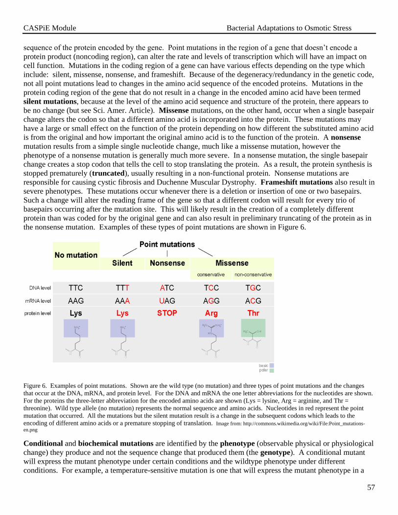
CASPiE Module Bacterial Adaptations to Osmotic Stress
57
sequence of the protein encoded by the gene. Point mutations in the region of a gene that doesn’t encode a
protein product (noncoding region), can alter the rate and levels of transcription which will have an impact on
cell function. Mutations in the coding region of a gene can have various effects depending on the type which
include: silent, missense, nonsense, and frameshift. Because of the degeneracy/redundancy in the genetic code,
not all point mutations lead to changes in the amino acid sequence of the encoded proteins. Mutations in the
protein coding region of the gene that do not result in a change in the encoded amino acid have been termed
silent mutations, because at the level of the amino acid sequence and structure of the protein, there appears to
be no change (but see Sci. Amer. Article). Missense mutations, on the other hand, occur when a single basepair
change alters the codon so that a different amino acid is incorporated into the protein. These mutations may
have a large or small effect on the function of the protein depending on how different the substituted amino acid
is from the original and how important the original amino acid is to the function of the protein. A nonsense
mutation results from a simple single nucleotide change, much like a missense mutation, however the
phenotype of a nonsense mutation is generally much more severe. In a nonsense mutation, the single basepair
change creates a stop codon that tells the cell to stop translating the protein. As a result, the protein synthesis is
stopped prematurely (truncated), usually resulting in a non-functional protein. Nonsense mutations are
responsible for causing cystic fibrosis and Duchenne Muscular Dystrophy. Frameshift mutations also result in
severe phenotypes. These mutations occur whenever there is a deletion or insertion of one or two basepairs.
Such a change will alter the reading frame of the gene so that a different codon will result for every trio of
basepairs occurring after the mutation site. This will likely result in the creation of a completely different
protein than was coded for by the original gene and can also result in preliminary truncating of the protein as in
the nonsense mutation. Examples of these types of point mutations are shown in Figure 6.
Figure 6. Examples of point mutations. Shown are the wild type (no mutation) and three types of point mutations and the changes
that occur at the DNA, mRNA, and protein level. For the DNA and mRNA the one letter abbreviations for the nucleotides are shown.
For the proteins the three-letter abbreviation for the encoded amino acids are shown (Lys = lysine, Arg = arginine, and Thr =
threonine). Wild type allele (no mutation) represents the normal sequence and amino acids. Nucleotides in red represent the point
mutation that occurred. All the mutations but the silent mutation result is a change in the subsequent codons which leads to the
encoding of different amino acids or a premature stopping of translation. Image from: http://commons.wikimedia.org/wiki/File:Point_mutations-
en.png
Conditional and biochemical mutations are identified by the phenotype (observable physical or physiological
change) they produce and not the sequence change that produced them (the genotype). A conditional mutant
will express the mutant phenotype under certain conditions and the wildtype phenotype under different
conditions. For example, a temperature-sensitive mutation is one that will express the mutant phenotype in a

CASPiE Module Bacterial Adaptations to Osmotic Stress
58
certain temperature range but will display the wildtype phenotype outside of that temperature range.
Biochemical mutations result in a non-functional protein product that creates a block in an enzymatic pathway.
An example of this is a mutation in a gene that codes for an enzyme important to the synthesis of proline in the
cell. If this mutation results in a non-functional protein product, than this enzyme will not be produced, and
since this enzyme is needed to make proline, the cell will not be able to make proline on its own using this
particular pathway. The auxotrophs we used last week and will observe today are examples of biochemical
mutations.
As mentioned earlier, there are a variety of means by which a mutation can occur: spontaneously or induced.
Spontaneous mutation occur during the normal cellular process of replication or as a result of transposons with
are mobile genetic elements. Induced mutations are caused by agents known as mutagens that are either
chemical or physical in nature and lead to damage to DNA. Physical mutagens include UV light and X ray
over-exposure which alters the physical structure of the DNA as a whole molecule or can cause the deletion of
bases. Chemical mutagens exert their effects by a variety of means depending on their chemical nature.
Chemical mutagens that are structurally similar to nucleotide bases are known as base analogs. These mutagens
can substitute for the bases, but do not form proper basepairs. An example of a base analog is 5-bromouracil
which is an analog for thymine but can lead to the erroneous basepairing with guanine. This will result in a
single basepair substitution in daughter cells. Chemicals such as acridine orange are known as intercalating
agents that insert themselves between bases, leading to basepair insertions or deletions. DNA-modifying
agents change the structure of a base so that it doesn’t basepair properly which can lead to a transition to a
different base with subsequent rounds of replication. An example of this is the alkylating agent
ethylmethanesulfonate (EMS) which adds methyl groups to guanine. This alteration to guanine can cause it to
mispair with thymine.
In order for cells to survive and be healthy, mutations must be kept to a minimum. If a complete round of
replication is finished, any mutations, spontaneous or induced, that aren’t detected and fixed will persist and
remain in the genome to be passed along in subsequent rounds of replication. To minimize this, cells have
DNA proofreading/editing and repair mechanisms that detect and repair damaged nucleotides or nucleotide
sequence. There are several enzymes that are involved in the actual repair. Different enzymes mediate
different types of repair, some examples of which result in excision of the damaged region, directly repairing
the nucleotide base, or fixing mismatched bases (excision and replacement). Because the enzymes that mediate
the repair are proteins themselves, any compromising mutations in their genes can lead to an accumulation of
mutations in the cell.
2. Pre-laboratory activities
Make sure that you have your observations and conclusions (comparison of your predictions to your
observation) from the auxotrophy and osmotic stress experiment plates recorded in your lab notebook. In
addition, answer the following questions in your lab notebook: (1) In the auxotrophy experiment, what was
the purpose of the plate that contained all of the supplements (ura, pro, and his)?, (2) In the auxotrophy
experiment, what was the purpose of the plate with no supplements added? and (3) In the osmotic stress
experiment, what was the purpose of the plate without salt (+ proline and + gb)?
● Read the introduction and the procedures for Laboratory Period 4 in this section of the lab manual.
● Where indicated in bold, work out calculations for any solutions to be made or diluted and answer any
questions posed.
● Before the lab period log onto Blackboard and take the pre-lab quiz for this week.

CASPiE Module Bacterial Adaptations to Osmotic Stress
59
3. Materials
Spectrophometry:: Determination of maximum absorbance:
Equipment and materials
●Spectrophotometers
●Cuvettes (2/group)
●test tube rack ●P-1000 micropipeter
●P-1000 micropipette tips
●beaker
●Liquid waste containers
●Squirt bottles of water
●Kim wipes
●Sharpies
●water
Reagents
●Stock solution of blue water (Stock A)
●1:1 dilution of Stock A (Stock B)
Spectrophotometry:: Measuring bacterial growth rates
Equipment and materials
●Spectrophotometers
●Cuvettes (2/group)
●Test tube rack ●125 ml Erlenmeyer flasks
●Sharpies
●Squirt bottles of water
●Kim wipes
●Liquid waste containers
●Sterile glass 5 ml volumetric pipettes
●Pipette bulbs
●Bunsen burner
●Sparker
●37ºC shaking incubator
Reagents
●Sterile M63 glucose + 0.1 mM proline broth
●Wildtype and 6 ProP mutant overnight M63 cultures
Quadrant streaking for pure culture
Equipment and materials
● Inoculating loops
● Bunsen burner
● Striker
● 30°C incubator
● LB plates
Reagents
● LB plate with quadrant streaked mixed culture (Escherichia coli, Serratia marcescens, and Bacillus
cereus) from last week
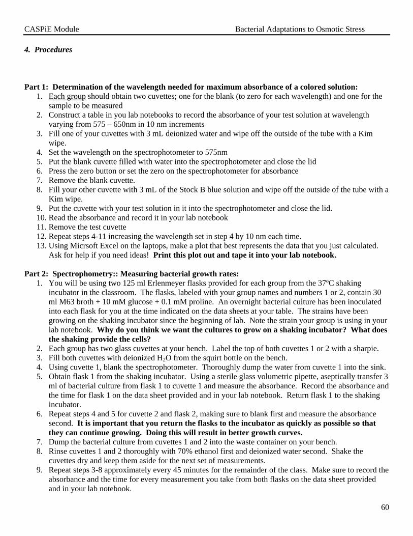
CASPiE Module Bacterial Adaptations to Osmotic Stress
60
4. Procedures
Part 1: Determination of the wavelength needed for maximum absorbance of a colored solution:
1. Each group should obtain two cuvettes; one for the blank (to zero for each wavelength) and one for the
sample to be measured
2. Construct a table in you lab notebooks to record the absorbance of your test solution at wavelength
varying from 575 – 650nm in 10 nm increments
3. Fill one of your cuvettes with 3 mL deionized water and wipe off the outside of the tube with a Kim
wipe.
4. Set the wavelength on the spectrophotometer to 575nm
5. Put the blank cuvette filled with water into the spectrophotometer and close the lid
6. Press the zero button or set the zero on the spectrophotometer for absorbance
7. Remove the blank cuvette.
8. Fill your other cuvette with 3 mL of the Stock B blue solution and wipe off the outside of the tube with a
Kim wipe.
9. Put the cuvette with your test solution in it into the spectrophotometer and close the lid.
10. Read the absorbance and record it in your lab notebook
11. Remove the test cuvette
12. Repeat steps 4-11 increasing the wavelength set in step 4 by 10 nm each time.
13. Using Micrsoft Excel on the laptops, make a plot that best represents the data that you just calculated.
Ask for help if you need ideas! Print this plot out and tape it into your lab notebook.
Part 2: Spectrophometry:: Measuring bacterial growth rates:
1. You will be using two 125 ml Erlenmeyer flasks provided for each group from the 37ºC shaking
incubator in the classroom. The flasks, labeled with your group names and numbers 1 or 2, contain 30
ml M63 broth + 10 mM glucose + 0.1 mM proline. An overnight bacterial culture has been inoculated
into each flask for you at the time indicated on the data sheets at your table. The strains have been
growing on the shaking incubator since the beginning of lab. Note the strain your group is using in your
lab notebook. Why do you think we want the cultures to grow on a shaking incubator? What does
the shaking provide the cells?
2. Each group has two glass cuvettes at your bench. Label the top of both cuvettes 1 or 2 with a sharpie.
3. Fill both cuvettes with deionized H2O from the squirt bottle on the bench.
4. Using cuvette 1, blank the spectrophotometer. Thoroughly dump the water from cuvette 1 into the sink.
5. Obtain flask 1 from the shaking incubator. Using a sterile glass volumetric pipette, aseptically transfer 3
ml of bacterial culture from flask 1 to cuvette 1 and measure the absorbance. Record the absorbance and
the time for flask 1 on the data sheet provided and in your lab notebook. Return flask 1 to the shaking
incubator.
6. Repeat steps 4 and 5 for cuvette 2 and flask 2, making sure to blank first and measure the absorbance
second. It is important that you return the flasks to the incubator as quickly as possible so that
they can continue growing. Doing this will result in better growth curves.
7. Dump the bacterial culture from cuvettes 1 and 2 into the waste container on your bench.
8. Rinse cuvettes 1 and 2 thoroughly with 70% ethanol first and deionized water second. Shake the
cuvettes dry and keep them aside for the next set of measurements.
9. Repeat steps 3-8 approximately every 45 minutes for the remainder of the class. Make sure to record the
absorbance and the time for every measurement you take from both flasks on the data sheet provided
and in your lab notebook.

CASPiE Module Bacterial Adaptations to Osmotic Stress
61
10. After you have taken your last measurement, leave the data sheet behind. Make sure your cultures are
still shaking on the incubator. We may need to take additional readings after you leave depending on
how the strains are growing.
**Leave space in your lab notebook at the end of this exercise. You will be provided with a class data set
after lab, and there will be further analysis to put in the conclusions section of this exercise.
Part 3. Streaking for a pure culture
REMEMBER TO PRACTICE APPROPRIATE ASEPTIC TECHNIQUE!
1. Find your LB plates with quadrant streaked mixed culture and bring them to your bench.
2. Each person in the group should obtain a fresh LB plate to quadrant streak a single, isolated
colony from the mixed culture plate onto. In groups of three, have each person select a different
type of bacteria to streak out to pure culture. In groups of two, choose which two types of bacteria
to streak out. You can ask us about good candidates to use on your plate.
3. Carefully label your fresh LB plate with your initials, the date, the type of media, and the type of
bacteria you will be streaking onto it.
4. Using aseptic technique select an isolated colony from the mixed culture plate and quadrant streak
it onto the new LB plate.
5. Invert the plate and put it into the 30o incubator. You will need to come back on Friday to pull
your plate from the incubator and make your observations.
5. Post-laboratory analysis and results
Plot the bacterial growth curve data in Excel and print it out and tape it in your lab notebook. You need to
come back on Friday to pull your plate from the incubator and make your observations. Did you get a
pure culture?
6. Preparation for the Next Laboratory Activity
You should read the introduction and procedures before going to your next laboratory period.
Perform any calculations in your lab notebook as indicated in the procedures portion of Laboratory 5
Take the online pre-lab quiz

CASPiE Module Bacterial Adaptations to Osmotic Stress
62
VI. Laboratory Period 5 – Quantification of substances in solution with
spectrophotometry and mutagenesis
Objectives
At the end of this laboratory period the students will be able to:
1. Create and use a standard curve generated with spectrophometry
2. Perform serial dilutions from stock solutions.
3. Calculate dilution factors for various steps along a serial dilution
4. Determine the concentration of an unknown solution using a standard curve
5. Understand the impact that mutations have on proteins and the function of cells
6. Understand DNA editing and repair
7. Describe various types of mutagenesis
1. Introduction
A .Introduction for Parts 1 and 2 of the procedures
Utility of the spectrophotometer to quantify levels of substances in solution:: The standard curve to
determine the concentration of an unknown
Recall from last week that an important experimental use of the spectrophotometer is to estimate an unknown
concentration of a substance in solution. This can be done in two ways. The first is by measuring the
absorbance of the solution and directly applying the Beer-Lambert Law. By choosing a wavelength that will be
maximally absorbed by the substance, the amount of light that is absorbed by the sample is proportional to the
concentration of the substance in solution, according to the Beer-Lambert Law:
A = ebc (Equation 3 from Lab 4)
where A is the absorbance (no units since A = log10 P0/P), e is the molar absorbtivity (L/ mole cm, a
fundamental property of the substance in question), b is the path length (cm, the width of the cuvette), and c is
the concentration of the substance in solution (mole/ L).
However, one does not always know e for a given substance. Therefore, a second method commonly used is to
interpolate from the linear range of an Absorbance vs. Concentration relationship that is constructed from the
absorbances of known concentrations of the substance in question. This relationship is known as a standard
curve, an example of which is shown in Figure 1. Using the standard curve in Figure 1 constructed from known
concentrations of Substance A, one could estimate an unknown concentration of Substance A in solution. It is
important to work within the linear range of the standard curve where the absorbance measurements are most
accurate. For example, if you obtained an absorbance measurement of 2 with your unknown solution of
Substance A, then interpolating from the standard curve you would get an estimate of 0.4 mM for the
concentration of Substance A. For a precise concentration estimate, the equation for the line (y = mx + b) that
best fits the data in the linear portion of standard curve would be used to solve for x (the concentration).
The linear relationship between Absorbance and concentration according to the Beer-Lambert Law is valid until
high concentrations of the substance in question as can be seen in Figure 1 (left) below.

CASPiE Module Bacterial Adaptations to Osmotic Stress
63
Figure 1. Examples of a spectrophotometric standard curve. On the right is an example of a standard curve constructed from
measuring the absorbance of solutions of known concentrations of Substance A. On the right is the same graph with an interpolation
of concentration of a solution of unknown concentration of A.
Serial dilutions and dilution factors
In lab period 2 we learned about simple, independent dilutions such as those that would be made from a stock
solution to give a diluted concentration in the final solution. This works well over a range of final
concentrations of the diluted substance. Sometimes, however, the final concentration needs to be very low. To
perform such a dilution in a one-step, independent fashion would require a very large volume of the final
solution to dilute into. This is impractical and wasteful! In this case, a dependent, serial dilution would be
appropriate.
A serial dilution is a dilution that takes place over a series of identical dilutions and results in a geometric
progression in the dilution factor with each dilution. A serial dilution consists of a set volume of solution
(aliquot) that is moved into a set volume of diluent. Using the example below in Figure 2, after the first dilution
we have performed a 1:10 (10-fold or dilution factor 10) dilution. Recall:
Dilution factor (DF) = total volume (diluent + aliquot)/aliquot volume. (Equation 1)
After this first round of dilution, an aliquot of solution is now moved from this diluted stock and moved into a
fresh set of diluent. To calculate the dilution factors in serial dilutions, we make use of the fact that we are
performing the same dilution repeatedly.
DF = DF1 x DF2 x DF3 x … (Equation 2)
So, after the second round we have now performed a
1:100 (100-fold) dilution (DF = 10 x 10). This is
repeated until the final concentration is achieved. With
this technique the original stock solution was diluted
10,000-fold in only 4 dilution steps! Not only is this
type of dilution useful to create a small volume of
dilute solutions from a stock, but it provides a quick
way to get a concentration series.
Figure 2. Example of a serial dilution. Note the transfer of a constant
volume to a constant volume along the series. A nice animation of a serial dilution can be found at:
http://education.wichita.edu/saltymicro/ecology_interactives/serial_dilution.html
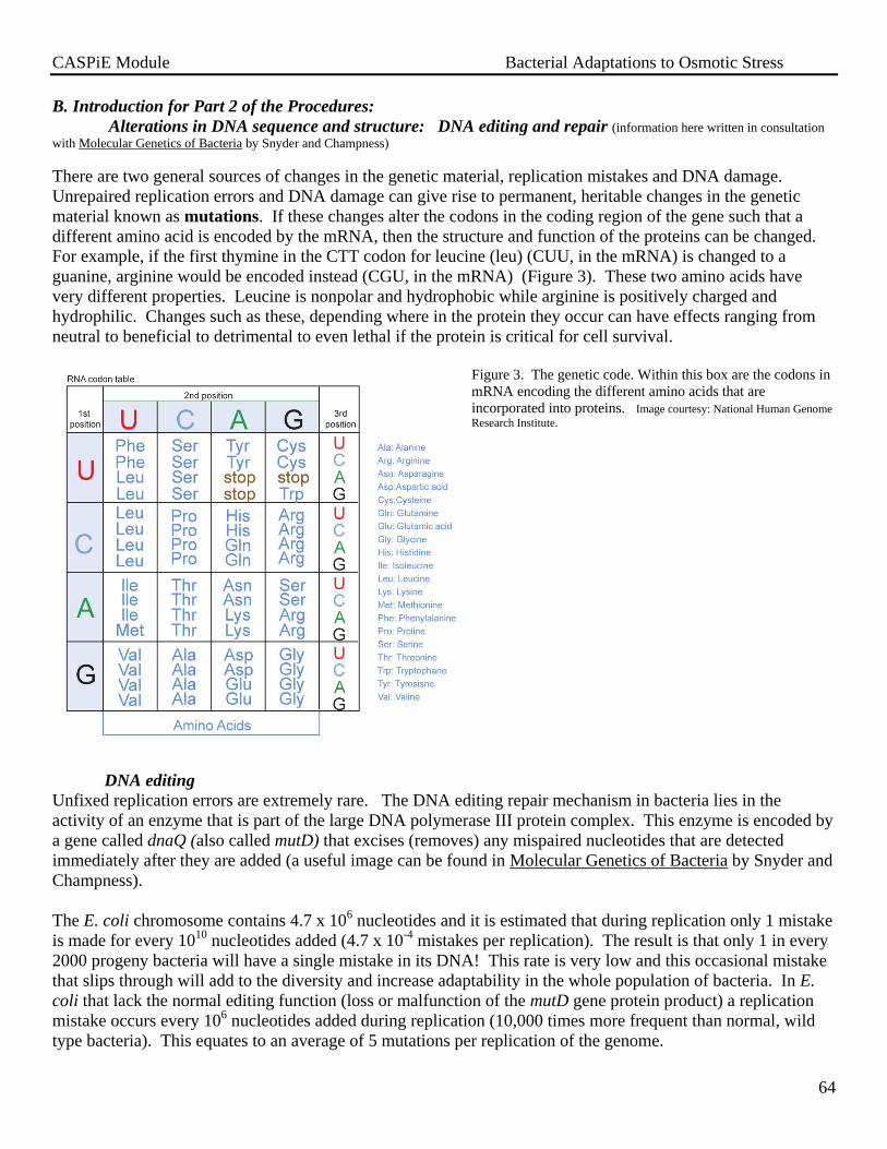
CASPiE Module Bacterial Adaptations to Osmotic Stress
64
B. Introduction for Part 2 of the Procedures:
Alterations in DNA sequence and structure: DNA editing and repair (information here written in consultation
with Molecular Genetics of Bacteria by Snyder and Champness)
There are two general sources of changes in the genetic material, replication mistakes and DNA damage.
Unrepaired replication errors and DNA damage can give rise to permanent, heritable changes in the genetic
material known as mutations. If these changes alter the codons in the coding region of the gene such that a
different amino acid is encoded by the mRNA, then the structure and function of the proteins can be changed.
For example, if the first thymine in the CTT codon for leucine (leu) (CUU, in the mRNA) is changed to a
guanine, arginine would be encoded instead (CGU, in the mRNA) (Figure 3). These two amino acids have
very different properties. Leucine is nonpolar and hydrophobic while arginine is positively charged and
hydrophilic. Changes such as these, depending where in the protein they occur can have effects ranging from
neutral to beneficial to detrimental to even lethal if the protein is critical for cell survival.
Figure 3. The genetic code. Within this box are the codons in
mRNA encoding the different amino acids that are
incorporated into proteins. Image courtesy: National Human Genome
Research Institute.
DNA editing
Unfixed replication errors are extremely rare. The DNA editing repair mechanism in bacteria lies in the
activity of an enzyme that is part of the large DNA polymerase III protein complex. This enzyme is encoded by
a gene called dnaQ (also called mutD) that excises (removes) any mispaired nucleotides that are detected
immediately after they are added (a useful image can be found in Molecular Genetics of Bacteria by Snyder and
Champness).
The E. coli chromosome contains 4.7 x 10⁶ nucleotides and it is estimated that during replication only 1 mistake
is made for every 1010
nucleotides added (4.7 x 10⁻⁴
mistakes per replication). The result is that only 1 in every
2000 progeny bacteria will have a single mistake in its DNA! This rate is very low and this occasional mistake
that slips through will add to the diversity and increase adaptability in the whole population of bacteria. In E.
coli that lack the normal editing function (loss or malfunction of the mutD gene protein product) a replication
mistake occurs every 106 nucleotides added during replication (10,000 times more frequent than normal, wild
type bacteria). This equates to an average of 5 mutations per replication of the genome.

CASPiE Module Bacterial Adaptations to Osmotic Stress
65
DNA repair
Changes in the composition and structure of the DNA can occur at any time and result from chemical or
physical agents that produce large or small alterations, as have been mentioned before. There are two types of
repair mechanisms for DNA damage: (1) general repair regardless of cause and resulting defect and (2) repair
for specific types of DNA alterations.
General repair mechanisms include mismatch repair, nucleotide excision repair, recombination repair and
the SOS inducible repair. Mismatch repair and nucleotide excision repair are ubiquitous repair mechanisms
found in all organisms and remove damage occurring on one strand of the DNA. Mismatch repair fixes DNA
alterations that lead to small distortions in the DNA resulting from base mismatches, frameshifts, incorporation
of base analogs and some types of alkylations. The mechanism involves recognizing mispaired nucleotides,
removing them, and then the missing nucleotides are replaced by DNA polymerase using the complementary
strand as a template. Defects in this process have been implicated in human cancers. In E. coli that lack DNA
editing and mismatch repair it is estimated that the rate of mutations is increased to 50 per replication.
Nucleotide excision repair is similar in general mechanism to mismatch repair, but is useful in repairing DNA
alterations that result in large distortions of the helix. It can repair most any type of damage, but especially that
resulting from UV irradiation.
Recombination repair is used when there is damage to both strands of the DNA in the same region. In this
situation there is no complementary strand to use as a template to fill in any excised sequence. In this case, if
replication has already happened, a strand from the same region from the newly produced DNA can serve as the
template to replace the damaged region of the parent. The SOS inducible repair response, as its name implies,
is turned on (induced) as a last ditch effort to save the cell and will not be discussed further in this course.
In addition to the general repair mechanisms, there are DNA repair mechanisms that are specific for certain
types of single base alterations. These mechanisms include repairs for base deamination, base alkylations,
guanine oxidations, and photoreactivation to repair UV damage.
A very common type of damage to DNA is the removal of amino groups (NH2) from bases in the nucleotide
(recall the structure of nucleotide: nitrogenous base and sugar phosphate backbone, Figure 4). This can occur
by chemical agents or spontaneously. Removal of amino groups can change the way bases pair with one
another which can lead to mutations if not fixed. For example, when adenine is deaminated it will pair with
cytosine instead of thymine ((a useful image can be found in Molecular Genetics of Bacteria by Snyder and
Champness).
Figure 4. The chemical structure of the two classes of
nucleotide bases in DNA. Image courtesy: National
Human Genome Research Institute.

CASPiE Module Bacterial Adaptations to Osmotic Stress
66
There are two types of repair mechanisms for deaminated bases: DNA glycosylase and Very Short Patch
(VSP) repair. DNA glycosylases are a group of enzymes that recognize damaged forms of specific bases. The
DNA glycosylases remove the damaged base from the sugar in the nucleotide and then another type of enzyme
(AP endonuclease) removes the rest of the nucleotide and DNA polymerase can insert a new, correct base in
that gap (a useful image can be found in Molecular Genetics of Bacteria by Snyder and Champness). VSP
repair is very specific for repairing mismatches that result from deamination of a form of cytosine that changes
it to thymine. This will lead to a mismatch of thymine with guanine. The basic repair mechanism for this type
of damage is to excise small patch of sequence (5 nucleotides) which can then be resynthesized by DNA
polymerase.
Some chemical mutagens damage DNA by adding chemical groups to portions of the nucleotides. Alkylating
agents add alkyl groups (CH3 (methyl group), for example) to bases and phosphates. An example of an
alkylating agent is the EMS we used in the chemical mutagenesis some you may perform this week. The most
likely targets for alkylation are nitrogens in guanine and adenine and oxygens in guanine and thymine (a useful
image can be found in Molecular Genetics of Bacteria by Snyder and Champness). These additions to the
nucleotides can alter their base pairing, distort the DNA helix and lead to mutations. One way of fixing this
damage is with the use of DNA glycosylases in a manner to that described for fixing deaminated bases. Special
proteins (methyltransferases) can be employed which simply transfer the alkyl group from the nucleotide to
themselves.
UV irradiation can damage DNA by causing the pyrimidine bases portions of adjacent thymines or cytosines to
fuse with one another leading to dimers in response to the absorption of the UV energy (a useful image can be
found in Molecular Genetics of Bacteria by Snyder and Champness).
These abnormal base linkages will disrupt the basepairing of the affected nucleotides and distort the DNA.
Because this type of damage is unavoidable by all organisms exposed to sunlight, a special repair system, called
photoreactivation , evolved to address it. In this repair system the dimeric bases are separated from one
another by the enzyme, photolyase (a useful image can be found in Molecular Genetics of Bacteria by Snyder
and Champness). Photolyase actually uses the energy from UV radiation (350-500 nm wavelength) to separate
fused bases from one another! Sometimes these dimers can be removed with the DNA glycosylases previously
described.
Aerobic metabolism yields large amounts of ATP to fuel cellular processes, but also leads to the formation of
reactive oxygen species, known as oxygen radicals. These radicals are highly reactive because they have an
extra electron(s) in their outermost electron shell. The most common form of damage to DNA from oxygen
radicals is guanine oxidations leading to 8-oxodG formation. This form of guanine, if left unrepaired, will
mispair with adenine and can lead to heritable mutations. A three-pronged repair strategy is employed to deal
with this damage which involves the protein products of the mutT, mutY, and mutM genes (a useful image can
be found in Molecular Genetics of Bacteria by Snyder and Champness). The mutM gene encodes a glycosylase
that removes the oxidized guanine to allow repair in a manner similar to the glycosylases mentioned above.
The mutY gene also encodes a glycosylase, but it removes the adenine that mistakenly pairs with the oxidized
guanine. The mutT gene encodes a phosphatase (an enzyme that removes phosphate groups from substrates)
that prevents the oxidized guanine from being incorporated into DNA to begin with. It does so by removing
one phosphate from the base to convert it from GTP (guanine tri-phosphate) to GDP (guanine di-phosphate)
which cannot be incorporated into the DNA. Very similar mechanisms for repair of oxidized guanine exist in
diverse organisms and it is thought the defects in them are the cause of some age-related cancers in humans.
This week we will be performing mutagenesis on S. typhimurium auxotrophs whose sole means of obtaining
proline is by uptake via ProP. An inhibitory concentration of glycine betaine will be used to select for mutant
bacteria that can overcome this antagonism and still transport proline. The types of mutagens you can choose

CASPiE Module Bacterial Adaptations to Osmotic Stress
67
from are: spontaneous, chemical (EMS), and using the auxotroph strain that has a defect in one of the DNA
repair enzymes.
2. Pre-laboratory activities
Make sure that you have your observations and conclusions (comparison of your predictions to your
observation) from the quadrant streak plating you did from your mixed culture last week.
● Read the introduction and the procedures for Laboratory Period 5 in this section of the lab manual.
● Where indicated in the procedures sections in bold, work out calculations for any solutions to be made or
diluted and answer any questions posed.
● Before the lab period log onto Blackboard and take the pre-lab quiz for this week.
3. Materials
Spectrophometry:: Determination of maximum absorbance, construction of a standard curve and
interpolation of an unknown:
Equipment and materials
●Spectrophotometers
●Cuvettes (15/group)
●test tube rack ●5 mL volumetric pipettes
●beaker
●Liquid waste containers
●Squirt bottles of water
●Kim wipes
●Sharpies
●deionized water
Reagents
●Stock solution of blue water (Stock A)
●1:1 dilution of Stock A (Stock B)
●‘unknown’ dilution from Stock B
Mutagenesis:
Equipment and materials
●P-200 micropipeter
●P-20 micropipeter (for chemical mutagenesis)
●P-200 micropipette tips (sterile)
●P-20 micropipette tips (sterile)
●Hockey stick
●Bunsen burner
●Striker
●Sharpies
●Pipette tip waste containers
●Test tubes with cotton stopper
●Sterile filter paper discs (for chemical mutagenesis)
●Chemical fume hood (for chemical mutagenesis)
●Gloves (for chemical mutagenesis)
●Tweezers (for chemical mutagenesis)

CASPiE Module Bacterial Adaptations to Osmotic Stress
68
●37o C incubator
Reagents
●Overnight culture of TL 1673 (proline auxotroph; proP+ proU-, putP-)
●Overnight culture, mutator strains (TL 1673 w/ knockout of single DNA repair genes)
●M63 glucose plates + 0.1mM proline ●M63 glucose plates + 0.1mM proline + 2mM Glycine betaine
●Other M63 glucose + 0.1mM proline + 2mM Glycine betaine plates depending on group projects
●EMS (for chemical mutagenesis)
4. Procedures
Part 1: Determination of maximum absorbance, construction of a standard curve and interpolation of an
unknown (do this with your group):
Create a standard curve with serial dilutions (1:1)
1. Each group has 15 tubes in your test tube rack. You will have 14 samples to read (7 different
concentrations, in duplicate).
2. You will be performing a serial dilution of Stock solution B. Label each tube, in duplicate with dilution
factor 1-64.
a. Tube set 1 = 1
b. Tube set 2 = 2
c. Tube set 3 = 4
d. Tube set 4 = 8
e. Tube set 5 = 16
f. Tube set 6 = 32
g. Tube set 7 = 64
h. Blank
3. Make a table in your lab notebook to record the absorbance given for each sample in the dilution series.
4. Before coming to lab, write out the procedure for your serial dilution given the dilution factors
listed in Step 2 above. Keep in mind that we need at least 3 mL of sample to read in the
spectrophotometer.
5. After verifying your serial dilution strategy with one of us, perform your serial dilution.
6. Verify with us that your tubes look right.
7. Set the wavelength on the spectrophotometer to the wavelength at which you observed the maximum
absorbance in your experiment from last week.
8. Zero the transmittance with the left hand knob while there is no cuvette in the spectrophotometer.
9. Put the blank cuvette with water in the spectrophotometer and zero the absorbance with the right hand
knob.
10. Measure the absorbance of each of your samples and record it in your lab notebook
11. If your duplicates are more than 5% different from each other, repeat that set.
12. Construct a standard curve with Excel using the average absorbance that you observed for each dilution.
Use the dilution factors as the concentration value. Fit the linear portion of the relationship with a linear
regression trend line and save the equation for the line. We will show you how to do this if you haven’t
done it before. Print your standard curve out and tape it into your lab notebook.
Determine the ‘concentration’ of the unknown sample
1. Rinse out two of your cuvettes from your serial dilution and fill them with 3 mL of the unknown
solution (these are your duplicate samples).
2. Using the same wavelength you did to construct your standard curve and zero the spectrophotometer
with the cuvette blank filled with water.

CASPiE Module Bacterial Adaptations to Osmotic Stress
69
3. Measure and record the absorbance of your unknown sample duplicates.
4. Interpolate the dilution factor of your unknown using the equation for the linear regression line from
your standard curve. Record the dilution factor of the unknown in your lab notebook.
Part 2: Mutagenesis
REMEMBER TO PRACTICE APPROPRIATE ASEPTIC TECHNIQUE!
Each person will be spread plating onto their test plates from an undiluted culture. For the control plate,
each person will have two plates, one for undiluted culture and one for diluted culture! The specific
contents of these plates will depend on the experimental design of each group.
1. At your bench each group will have one tube of an overnight culture of the appropriate bacteria for
your experiment.
2. Each group should obtain three empty sterile glass or polystyrene tubes and a bottle of sterile M63
glucose + proline broth to use as a diluent.
3. The overnight cultures will contain roughly 109 cells in them and we want a final cell concentration
of 103 cells to spread plate on to our plates. Before coming to lab, calculate the aliquot volume
and diluent volume needed to perform 3, 100-fold serial dilutions with a final volume of 1 ml
at each step.
5. After checking your calculations with us, perform the dilution of the bacteria. Don’t forget to label the
tubes carefully!
6. At your bench, each person will have one test plate and two control plates.
**Each person will spread plate the following with the appropriate bacteria:
1. Test plate (M63 glu + 0.1 mM pro + 2mM GB) – undiluted culture
2. Control plate (M63 glu + 0.1 mM pro) – undiluted culture
3. Control plates (M63 glu _ 0.1mM pro) – diluted culture (1 each for 107, 10
5, and 10
3 cells)
Spontaneous mutagenesis
1. Each person should label their plates with their initials, the bacterial strain, the media, the estimated cell
concentration, the type of mutagenesis (spontaneous), and the date.
2. Using aseptic technique, spread plate 100 µL of your diluted and undiluted bacteria onto the
appropriate plates.
3. Invert the plates and place them in the 37o C incubator
4. Because this is a critical step in our series of experiments, we will come in to check on your plates and
put them in the refrigerator for you.
Chemical mutagenesis (we will handle the mutagen)
1. Each person should label their plates with their initials, the bacterial strain, the media, the estimated cell
concentration, the type of mutagenesis (chemical and the mutagen), and the date.
2. Using aseptic technique, spread plate 100 µL of your diluted and undiluted bacteria onto the
appropriate plates.
3. Using aseptic technique, transfer a sterile filter paper disc into the center of each of your plates with
tweezers.
4. Wearing gloves, in the chemical fume hood, we will pipette 10 µl EMS onto the filter paper disc on each
of your plates. Push the disc down into the agar some with the pipette tip. What additional control
should be done for this type of mutagenesis?
5. Invert the plates and place them in the 37o C incubator
CASPiE Module Bacterial Adaptations to Osmotic Stress
70
6. Because this is a critical step in our series of experiments, we will come in to check on your plates and
put them in the refrigerator for you.
Mutator strain mutagenesis
1. Each person should label their plates with their initials, the bacterial strain, the media, the estimated cell
concentration, the type of mutagenesis (mutator and the strain), and the date.
2. Using aseptic technique, spread plate 100 µL of your diluted and undiluted bacteria onto the
appropriate plates.
3. Invert the plates and place them in the 37o C incubator
4. Because this is a critical step in our series of experiments, we will come in to check on your plates and
put them in the refrigerator for you.
5. Post-laboratory analysis and results
We will be coming in to remove your plates from the incubator and will place them in the refrigerator in the lab.
You need to come in early next week and look at your plates and write down your observations in your lab
notebook.
6. Preparation for the Next Laboratory Activity
You should read the introduction and procedures before going to your next laboratory period.
Perform any calculations in your lab notebook as indicated in the procedures portion of Laboratory 6
Take the online pre-lab quiz

CASPiE Module Bacterial Adaptations to Osmotic Stress
71
VII. Laboratory Period 6 – Pinwheel streaking technique, mutational frequency
estimations, inoculation of liquid media, and the theory of transduction
Objectives
At the end of this laboratory period the students will be able to:
1. Understand the usefulness of pinwheel streaking
2. Pinwheel streak bacterial stocks of mutants
3. Estimate the mutational frequency in each mutagenesis condition
3. Inoculate liquid media with a single colony
5. Describe the process of generalized transduction as a means for transfer of genetic information
between organisms in the laboratory
1. Introduction
A .Introduction for Part 1 of the procedures
Pinwheel streaking for isolated colonies -- multiple colony sources
Pinwheel streaking is a variation on the technique of streaking for isolated colonies. Previously when you used
the quadrant streaking technique to streak for isolated colonies, you did so using an entire plate. This is a good
technique to do if you are streaking out an important bacterial culture that you will be using a lot in your
research. As you have seen, quadrant streaking, when done correctly, results in many single isolated colonies
that can be picked and inoculated into liquid culture or streaked onto more solid media for research purposes.
However, what happens when you have a bunch of different colonies you have created from an experiment like
our mutagenesis? You could get well over 100 single colonies, and you may need to screen through these for
those colonies that have the phenotype you desire. Streaking each of those single colonies individually onto a
whole plate would take a lot of time and would be a huge waste of resources. Instead of doing that, you can use
the pinwheel streaking technique that basically divides the plate into a pinwheel. Single colonies from a plate
can be selected with a fine needle (inoculating needle) and streaked for isolated colonies on a smaller scale in
each segment of the pinwheel using the same basic technique to dilute the bacteria down in quadrant streaking.
A diagram showing an example of the pinwheel streak technique is shown below with the order of streaks
numbered 1-3. Successful pinwheel streaking will result in isolated colonies as shown at the bottom of the third
streak. This technique can be repeated in the nine remaining sections of the pinwheel pattern.
12
3
Figure 1. Example of the pinwheel streak technique with the
order of streaks indicated as 1-3.

CASPiE Module Bacterial Adaptations to Osmotic Stress
72
B. Introduction for Part 2 of the procedures:: Mutation frequency estimation
The S. typhimurium genome is a circular chromosome that contains roughly 4,857,432 base pairs (Figure 2).
Figure 2. - The circular chromosome of Salmonella Typhimurium. The base pair count is indicated in black along the outer edge of the circle. The
two, multicolored outer circles in the map are the forward strand (outer ring) and the reverse strand (inner ring) of the chromosome. Red genes are
those that have homologs shared between 8 compared Salmonella serotypes (S. typhi, S. paratyphi A, S. paratyphi B, S. arizonae or S. bongori).
Green genes are those that are shared with at least one other of the 8 Salmonella serotypes, but not with some strains of E. coli and K. pneumoniae.
The blue genes are specific to S. typhimurium. Grey represents other combinations. The inner black and purple/yellow rings are related to G+C
content and bias. Reprinted by permission from Macmillan Publishers Ltd: [Nature] (Michael McClelland, Kenneth E. Sanderson, John Spieth, Sandra W. Clifton,
Phil Latreille et al. Complete genome sequence of : Salmonella enterica: serovar Typhimurium LT2 Oct 25;413(6858):852-6), copyright (2001)
This entire chromosome is replicated before each cell division and the fidelity in this process is very high.
Recall from lab #5 that the spontaneous mutation rate is estimated to be very low (once in every 1010
nucleotides added or ~4.7 x 10⁻⁴
mistakes per replication). In E. coli this results in one bacterium in every 2000
progeny being produced having a single nucleotide mistake. As an example, the mutator strain bacteria with the
mutT repair enzyme defect have been estimated to produce mistakes 100-10,000 times more often than wild
type bacteria (Maki and Sekiguchi, 1992).
Within the 4.8 x 10⁶ nucleotide base pairs of the S. typhimurium chromosome are 4,620 genes of which about
4,432 encode proteins (numbers from the NCBI website; McClelland et al., 2001). proP is one of those genes
and its protein coding region occupies a mere 1500 base pairs! Clearly, the chance that a mutation will be
observed within proP spontaneously is quite remote. The chances are higher in the mutator strains and induced
mutagenesis (UV exposure or chemically-induced).
Today we will get a better feel for the relationship between the mutation frequency rate based on the
mutagenesis type, as discussed above, and the observed mutation frequency rate based on our particular
environmental conditions. Because not all genetic mutations will be relevant and/or confer benefits to survival
in all environmental conditions, the overall mutation rate will be lower than predicted simply by mutagenesis
type.
Estimation of mutation frequency :: Bacterial Culture Titer Calculations
We can use the results of our platings last week to determine the mutation frequency in each in our
experimental conditions. This number is what fraction of the total available bacteria were able to grow in our
restrictive test conditions. Last week we streaked fully grown bacterial cultures onto our test and control plates.

CASPiE Module Bacterial Adaptations to Osmotic Stress
73
This results in the growth of a lawn on the control plates which results from a number of bacteria that we cannot
directly quantify. In order to calculate the number of living cells present in that overnight culture, we also
streaked a diluted sample of these cultures onto our control plates (no GB). By counting the number of cells
that grow on this plate and knowing the dilutions we made and the volume we plated, we can calculate the total
number of living bacteria present in the overnight culture. This is known as the bacterial titer and is usually
expressed as the # of bacteria cells present/ml of liquid, or more accurately as the # of colony forming units/ml
(c.f.u./ml). The formula for titer calculations is:
T = D x N x P
T – Bacterial Titer
D – Dilution Factor (Final Volume/Aliquot Volume)
N – Number of colonies on the plate
P – Plating Factor (1/Volume Plated)
The dilution factor, as you have previously learned, is equal to the final volume divided by the aliquot volume.
Each dilution has its own dilution factor. When multiple dilutions are present for a single titer calculation, as
was the case for ours, the dilution factors can be multiplied by each other to get a total dilution factor for the
calculation. The number of colonies on the plate is the number of single colonies that can be counted on the
plate. Ideally, this number should be between 30 and 300. The plating factor is 1 divided by the volume plated.
Since we plated 100μl, or 0.1ml, our plating factor is 1/0.1, for a plating factor of 10. An example of a titer
calculation is shown below:
An overnight bacterial culture is diluted for titer calculation as follows: 100μl of overnight culture is diluted into
900μl of diluent five times before 200μl is spread on a plate. A total of 79 colonies are counted (Figure 3).
Figure 3. Example of a plate used for titer calculation.
The original bacterial titer is calculated as:
T = (10x10x10x10x10) x 79 x 5 c.f.u./ml
T = (105) x 79 x 5 c.f.u./ml
T = 395 x 105 c.f.u./ml
T = 3.95 x 10⁷ c.f.u./ml
We will calculate the number of colony forming units present in our overnight bacterial cultures to help us
calculate and compare the mutational frequencies between spontaneous mutagenesis (TL 1673), the UV light
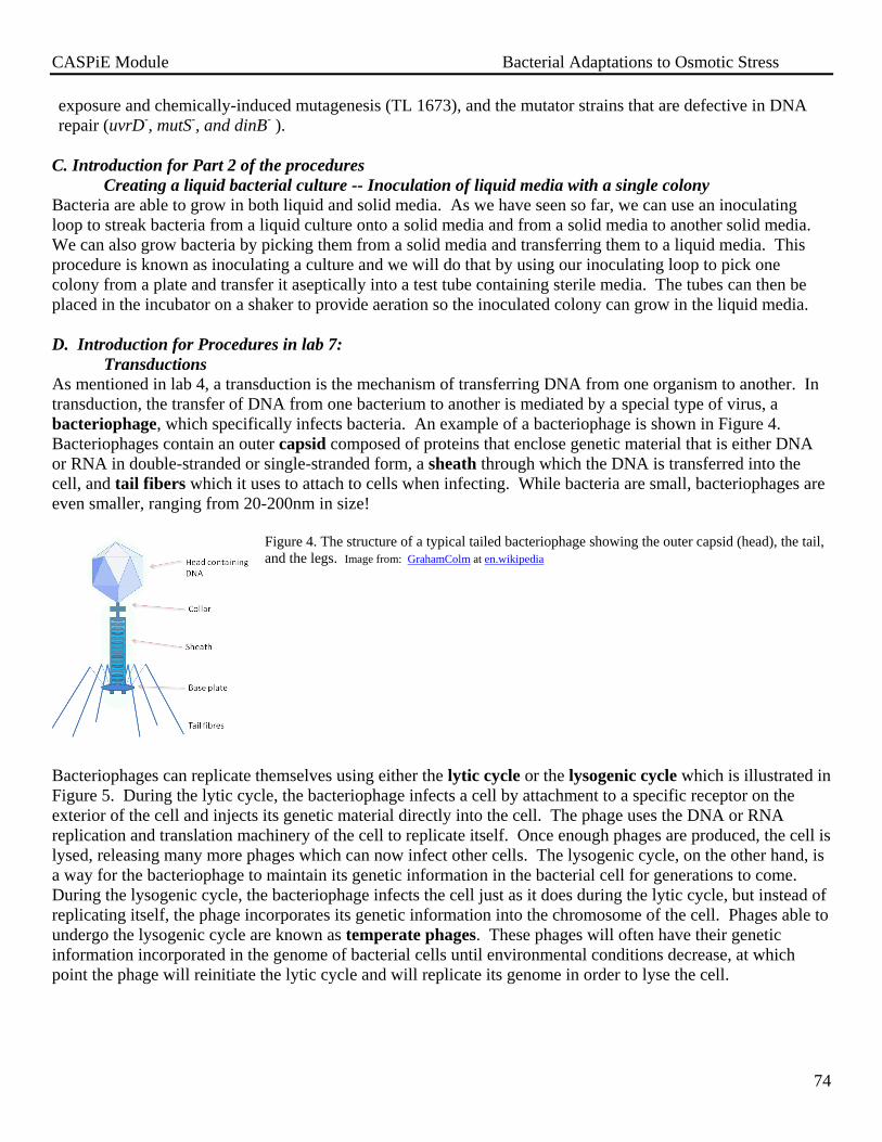
CASPiE Module Bacterial Adaptations to Osmotic Stress
74
exposure and chemically-induced mutagenesis (TL 1673), and the mutator strains that are defective in DNA
repair (uvrD-, mutS
-, and dinB
- ).
C. Introduction for Part 2 of the procedures
Creating a liquid bacterial culture -- Inoculation of liquid media with a single colony
Bacteria are able to grow in both liquid and solid media. As we have seen so far, we can use an inoculating
loop to streak bacteria from a liquid culture onto a solid media and from a solid media to another solid media.
We can also grow bacteria by picking them from a solid media and transferring them to a liquid media. This
procedure is known as inoculating a culture and we will do that by using our inoculating loop to pick one
colony from a plate and transfer it aseptically into a test tube containing sterile media. The tubes can then be
placed in the incubator on a shaker to provide aeration so the inoculated colony can grow in the liquid media.
D. Introduction for Procedures in lab 7:
Transductions
As mentioned in lab 4, a transduction is the mechanism of transferring DNA from one organism to another. In
transduction, the transfer of DNA from one bacterium to another is mediated by a special type of virus, a
bacteriophage, which specifically infects bacteria. An example of a bacteriophage is shown in Figure 4.
Bacteriophages contain an outer capsid composed of proteins that enclose genetic material that is either DNA
or RNA in double-stranded or single-stranded form, a sheath through which the DNA is transferred into the
cell, and tail fibers which it uses to attach to cells when infecting. While bacteria are small, bacteriophages are
even smaller, ranging from 20-200nm in size!
Figure 4. The structure of a typical tailed bacteriophage showing the outer capsid (head), the tail,
and the legs. Image from: GrahamColm at en.wikipedia
Bacteriophages can replicate themselves using either the lytic cycle or the lysogenic cycle which is illustrated in
Figure 5. During the lytic cycle, the bacteriophage infects a cell by attachment to a specific receptor on the
exterior of the cell and injects its genetic material directly into the cell. The phage uses the DNA or RNA
replication and translation machinery of the cell to replicate itself. Once enough phages are produced, the cell is
lysed, releasing many more phages which can now infect other cells. The lysogenic cycle, on the other hand, is
a way for the bacteriophage to maintain its genetic information in the bacterial cell for generations to come.
During the lysogenic cycle, the bacteriophage infects the cell just as it does during the lytic cycle, but instead of
replicating itself, the phage incorporates its genetic information into the chromosome of the cell. Phages able to
undergo the lysogenic cycle are known as temperate phages. These phages will often have their genetic
information incorporated in the genome of bacterial cells until environmental conditions decrease, at which
point the phage will reinitiate the lytic cycle and will replicate its genome in order to lyse the cell.

CASPiE Module Bacterial Adaptations to Osmotic Stress
75
Figure 5. Illustration of the lytic (left) and lysogenic (right)
cycles of bacteriophage-mediated transduction. Image by
Suly12 (Own work) [GFDL (www.gnu.org/copyleft/fdl.html), CC-BY-SA-
3.0 (www.creativecommons.org/licenses/by-sa/3.0/) or CC-BY-SA-2.5
(www.creativecommons.org/licenses/by-sa/2.5)], via Wikimedia Commons
Scientists take advantage of this naturally-occurring process to transfer genetic material from a specifically
selected bacterial strain to another selected bacterial strain. This common molecular biology technique takes
advantage of the lytic cycle and is known as a generalized transduction. Figure 6 illustrates the steps of a
generalized transduction. The first step of a generalized transduction is to infect a bacterial population that
contains genomic information you wish to transfer to another bacterial population. To do this, you infect a
culture of this population with a bacteriophage. The bacteriophage injects its DNA into the cell (step 1). The
information the phage injects into the cell codes for enzymes that degrade both the host and viral DNA (step 2).
To complete the lytic cycle, the phage incorporates chopped up DNA into the capsids of newly-made phage.
Most of the time, the phage will incorporate replicated phage DNA, but sometimes the phage will also
incorporate chopped up bacterial DNA into its capsid (step 3). The phage we will be using for our transductions
has been engineered so that it incorporates bacterial DNA more often than it normally would. The bacteria
containing these phages will then lyse and the newly-formed phages are released into the surrounding
environment. At this point, the phages produced are collected in what is known as a lysate. This lysate
contains all the phage that infected the original bacterial culture which will have their own phage DNA along
with some of the original bacterial host DNA. The phage-containing lysate can then be used to transduce a new
bacterial culture that serves as the recipient of the transferred genetic information. These phages will inject the
bacterial DNA into the new cell (step 4). This DNA is incorporated into the chromosome of the recipient strain
by recombination (step 5).
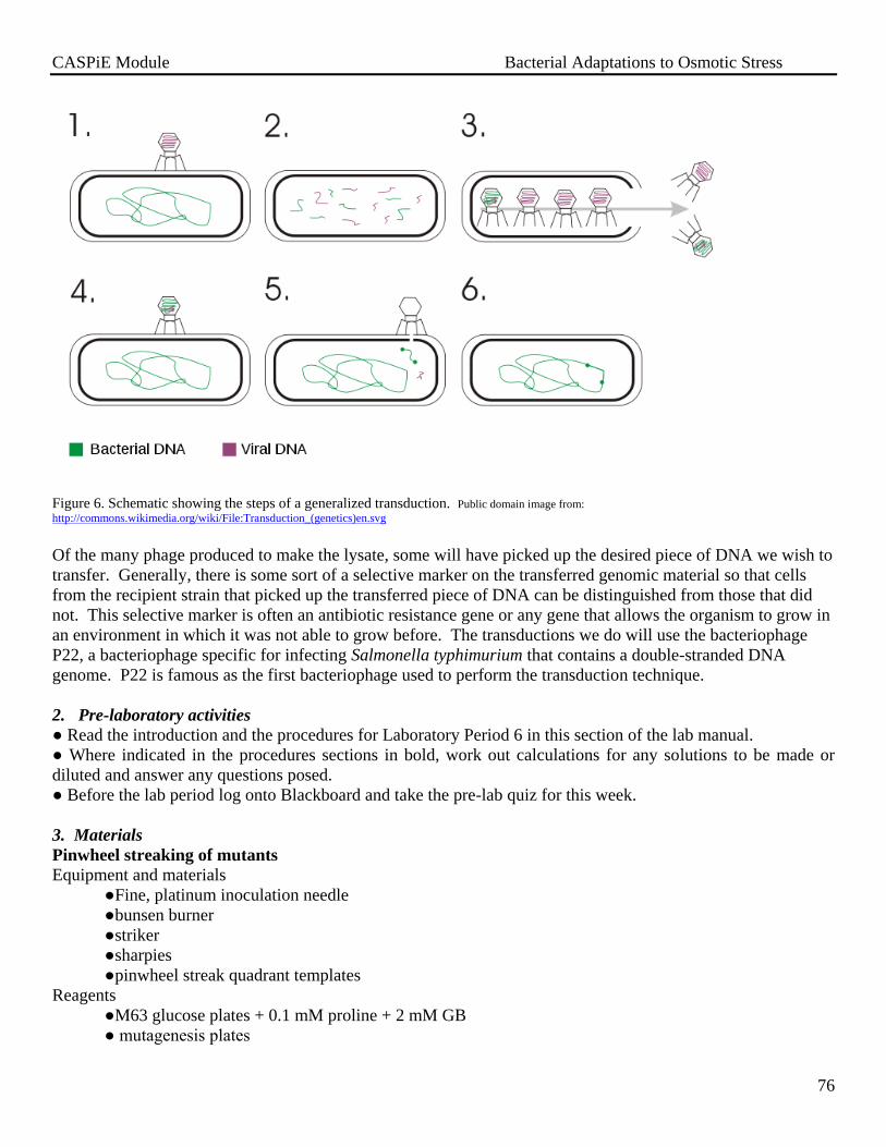
CASPiE Module Bacterial Adaptations to Osmotic Stress
76
Figure 6. Schematic showing the steps of a generalized transduction. Public domain image from:
http://commons.wikimedia.org/wiki/File:Transduction_(genetics)en.svg
Of the many phage produced to make the lysate, some will have picked up the desired piece of DNA we wish to
transfer. Generally, there is some sort of a selective marker on the transferred genomic material so that cells
from the recipient strain that picked up the transferred piece of DNA can be distinguished from those that did
not. This selective marker is often an antibiotic resistance gene or any gene that allows the organism to grow in
an environment in which it was not able to grow before. The transductions we do will use the bacteriophage
P22, a bacteriophage specific for infecting Salmonella typhimurium that contains a double-stranded DNA
genome. P22 is famous as the first bacteriophage used to perform the transduction technique.
2. Pre-laboratory activities
● Read the introduction and the procedures for Laboratory Period 6 in this section of the lab manual.
● Where indicated in the procedures sections in bold, work out calculations for any solutions to be made or
diluted and answer any questions posed.
● Before the lab period log onto Blackboard and take the pre-lab quiz for this week.
3. Materials
Pinwheel streaking of mutants
Equipment and materials
●Fine, platinum inoculation needle
●bunsen burner
●striker ●sharpies
●pinwheel streak quadrant templates
Reagents
●M63 glucose plates + 0.1 mM proline + 2 mM GB
● mutagenesis plates
CASPiE Module Bacterial Adaptations to Osmotic Stress
77
Mutation frequencies
Equipment and materials
●cell counter
●sharpie
●calculator
●laptop computer
Reagents
●mutagenesis test plates (full strength culture plating)
●control plates (diluted culture plating)
Inoculation of liquid media with a single colony
Equipment and materials
●Inoculation loop
●bunsen burner
●striker ●sharpies
Reagents
●Tubes of LB broth
● plate of bacteria
4. Procedures
Part 1: Pinwheel streaking of mutants
REMEMBER TO PRACTICE APPROPRIATE ASEPTIC TECHNIQUE!
1. Obtain an M63 glucose + 0.1 mM proline + 2 mM GB plate 2. Clearly label your plate with what you are streaking (i.e. Spontaneous mutants or EMS mutants or
Mutator Mutants), the type of media and supplements, your initials, and the date. 3. Using a sharpie, draw a small straight line on the back of your plate from the outside edge toward the
center of the plate. This line will serve as the starting point for your pinwheel streaking. 4. Take the pinwheel streaking template petri dish top provided for you and place your plate inside it,
making sure to line up the line you drew in step 3 with one of the lines of the pinwheel. 5. Turn on your Bunsen burner. 6. Remove the top of your plate. 7. Flame your fine platinum inoculation needle and pick up a colony from your mutagenesis plate from last
week. Close the lid on your mutagenesis plate. 8. In your first pinwheel pie slice, streak back and forth in a horizontal motion starting near the outer edge
and gradually moving inward 8-12 times as seen in step 1 of Figure 1. This streak should extend about
halfway down the quadrant. 9. Flame the inoculation needle and cool briefly by touching the middle of the plate. 10. Starting in the first section and extending downwards, streak 2-4 times back and forth in a vertical
motion as shown in step 2 of Figure 1. This streak should start in the first section and extend down
further towards the bottom of the quadrant. 11. Flame the inoculation needle and cool briefly by touching the middle of the plate. 12. Streak back and forth again in a horizontal manner through the bottom portion of the vertical streak you
made in step 10. This streak should extend down towards the bottom of the quadrant as shown for step
3 in Figure 1. 13. Repeat steps 7-12 for the remaining 9 quadrants, using a different mutant in each quadrant. 14. Put the top back on your plate, invert, and place in the 37°C incubator to grow. 15. We will remove the pinwheel streak plates for you before next week.
CASPiE Module Bacterial Adaptations to Osmotic Stress
78
Part 2: Mutation frequency estimations
1. Find your test and diluted culture control plates.
2. Count the number of colonies on each of your diluted platings on your control plates (no GB).
a. obtain a cell counter and a sharpie
b. count the number of colonies by marking the location of a single colony with a
sharpie and then make a single click on the cell counter.
c. repeat this for all colonies on the plate
3. Calculate the dilution factor for the dilution you performed last week to create the diluted tube of
cells.
4. How would you use the dilution factor and the number of colonies from the diluted culture that
grew on your control plates to calculate the titer of your cultures?
5. As you did in step 2, count the number of colonies on your test plates (full strength culture on test
plates).
6. Calculate the mutation frequency for your mutagenesis. How would you do this?
7. Enter your mutation frequency in your lab notebook and up on the board. How do all of the
mutation frequencies compare? Do the different frequencies make sense?
Part 3: Inoculation of liquid media with a single colony
REMEMBER TO PRACTICE APPROPRIATE ASEPTIC TECHNIQUE!
1. Obtain a tube of LB broth and label it with the culture you are inoculating, the type of media, your
initials, and the date.
2. Turn your Bunsen burner on.
3. Flame your inoculation loop and cool in the agar of the plate provided where no bacteria are present.
4. Pick up a single colony from the plate with your inoculation loop.
5. Aseptically remove the top of the tube with LB media and place the inoculation loop into the media.
You may need to delicately shake the loop in the tube to get the colony off.
6. Flame the tube again and put the cap back on.
7. Flame your loop BEFORE setting it back down on your bench top.
8. Incubate the tubes shaking at 37°C.
5. Post-laboratory analysis and results
You need to come in on Friday to check your pinwheel streak plates and make observations. You should also
get your inoculated liquid cultures from the incubator and make observations.
6. Preparation for the Next Laboratory Activity
● Each of you will need to come in on Monday of next week (February 28th
) and inoculate 10 tubes of
LB broth with a single colony from 10 of your pinwheel streak quadrants. We will give you more
instructions in lab.
● You should read the introduction and procedures before going to your next laboratory period.
● Perform any calculations in your lab notebook as indicated in the procedures portion of Laboratory 7
● Take the online pre-lab quiz

CASPiE Module Bacterial Adaptations to Osmotic Stress
79
VIII. Laboratory Period 7 – Genetic Mapping, Linkage, Transduction, and Gram staining
Objectives
At the end of this laboratory period the students will be able to:
1. Describe the general idea of recombination
2. Describe the general idea of genetic linkage
3. Understand the importance of the recombination frequency in genetic mapping
4. Describe the technique of genetic mapping
5. Understand the usefulness of phenotypic markers in genetic mapping
6. Describe the concept of cotransduction
7. Perform a generalized transduction
8. Perform a Gram stain
9. Visually identify gram-positive and gram-negative bacteria
1. Introduction
Last week you pinwheel streaked ten mutants onto a fresh M63 glucose plate with a previously inhibitory
concentration of glycine betaine. The next thing we want to do is determine which of those mutations are
actually in the proP gene. We can do that by taking advantage of the properties of transduction you learned
about last week and the properties of gene linkage described below.
Genetic Mapping and Linkage (information here written in consultation with Molecular Genetics of Bacteria by Snyder and Champness)
Genetic mapping is an important tool used by geneticists who work with all different organisms. In humans,
genetic mapping is often used to identify that a disease is linked to one or more genes. Mapping can tell us
exactly which chromosome a particular gene is on and exactly where it lies on that chromosome. Maps have
been used to locate the genes and mutations responsible for diseases such as cystic fibrosis, muscular dystrophy,
asthma, cancer, and even some psychiatric conditions (National Human Genome Research Institute,
www.genome.gov) (Figure 1). This type of mapping is also known as linkage mapping and it is the concept of
linkage that makes mapping possible. An image depicting the genetic loci of some human diseases that were
mapped using linkage can be found at http://genome.crg.es/courses/laCaixa05/GenesAndDisease/index.html.
Linkage occurs when two markers are sufficiently close together on the DNA that recombination between them
is less than optimum. In eukaryotes, this recombination often refers to the crossing over, or breaking and
joining of DNA that occurs during the process of meiosis. Figure 1 shows a schematic of the recombination
event.
Figure 1. Illustration of crossing-over and recombination during the formation of
gametes (germ cells) or meiosis. Crossing-over is part of a complicated process
which can occur during cell division. In meiosis, the precursor cells of the sperm
or ova must multiply and at the same time reduce the number of chromosomes to
one full set. During the early stages of cell division in meiosis, two chromosomes
of a homologous pair may exchange segments in the manner shown above,
producing genetic variations in germ cells. Image from: http://www.accessexcellence.org/RC/VL/GG/comeiosis.php

CASPiE Module Bacterial Adaptations to Osmotic Stress
80
The closer two genes are to each other, the smaller the space between them, and therefore the smaller possibility
of genetic recombination occurring. Therefore, two genes that are linked together will be more likely to remain
together during recombination events. On the other hand, two genes that are far apart have more distance
between them and therefore a greater likelihood of recombination occurring (Figure 2).
Figure 2. Schematic depicting the linkage of two, closely located genes on a
chromosome in eukaryotes. Shown are two chromosomes with alleles of
the same genes aligned next to each other. The A, B, and C alleles are on
one chromosome and the alleles a,b, and c are on the other. AB and ab are
located close to one another while gene Cc is further away. The chance is
high that AB and ab will remain together following a recombination event is
high due to their proximity. Image from: Wellcome Trust
http://genome.wellcome.ac.uk/doc_WTD020778.html
Linkage mapping is made possible through the use of genetic markers. A genetic marker is a gene or DNA
sequence with a known location on the chromosome. By analyzing the recombination frequency (the number
of times genes are separated following recombination occurs), we can determine how close the genes are to
each other. The smaller the recombination frequency is, the shorter the distance between the genes is.
Distances between genes are quantitated as map units, where each map unit represents a recombination
frequency of 1%.
A .Introduction for Part 1 of the procedures
In prokaryotes, mapping is also used to determine the location of a particular gene. It is often used to
investigate the gene responsible for the production of a mutant phenotype. A variety of methods can be used to
map locations of genes in bacteria. One commonly used method for precise mapping is by transduction with a
bacteriophage and selection for a specific marker that leads to some observable phenotype. These markers
often take the form of an antibiotic resistance cassette or a gene coding for the protein required to metabolize a
particular sugar as a carbon source. While markers come in many different varieties, they all share one thing in
common: they provide the organism with the tools necessary to grow where it was not able to grow before.
Using the transduction technique of mapping is based on whether the regions of the two genes of interest (the
gene being mapped and the selectable marker) can be cotransduced together. In other words, can the
bacteriophage packaging the host DNA fit both genes and the distance between them into its head during
transduction? The closer these two genes are to each other, the more likely that is to occur, and we should see
more transductants that have both the mutant type we are screening for and the selectable marker. In order to
map the mutations we have created, we will be using one transduction, the general steps of which are illustrated
below (Figure 3).

CASPiE Module Bacterial Adaptations to Osmotic Stress
81
Figure 3. Schematic of the basic steps in our transduction to map our
mutations to proP.
The genetic marker we will use is a tetracycline resistance cassette (TetR) inserted into the melA gene in the
original strain you mutagenized. This gene codes for the enzyme α-galactosidase that breaks down the sugar
melibiose and allows the cell to use melibiose as a sole carbon source. A strain with a disruption of melA with
Tet cannot grow on melibiose as a sole carbon source. However, the TetR gives the strain the ability to grow on
media containing Tet, a bacteriostatic antibiotic that would otherwise inhibit growth. The melA gene is in
relatively close proximity to the proP gene in our chromosome (shown in Figure 4). Because of this, the genes
are considered linked and some will co-transduce together.
0
Figure 4 – Schematic of the Salmonella typhimurium LT2 chromosome extending from bases 4,530,970 to 4,543,753
(http://blast.ncbi.nlm.nih.gov/Blast.cgi). This region contains the proP gene and the melA gene as well as the region in between, which contains 7
additional genes whose coding region is on the opposite strand, as indicated by the arrows. The P22 bacteriophage is capable of fitting 44,000
basepairs of DNA in its head, and the total distance between the proP and melA genes is 12,783 basepairs. This distance is large enough that some
phage will not be able to pick up both genes and the distance between them but also small enough so that some phage will.
proP melA

CASPiE Module Bacterial Adaptations to Osmotic Stress
82
In order to map which of the isolated mutants are in proP, you can make a lysate for all ten of your mutants.
The lysate contains bacteriophage P22 that grew up on each of your mutants. These bacteriophage carry the
genes from your mutants in their phage heads. Some of the phage will carry the TetR in the melA linked to the
proP from your mutant strain. Once you have the lysate, you can do a transduction into a recipient strain, TL
4513 (shown in Figure 5). TL 4515 is a proline auxotroph that lacks all of the transporters that take in proline,
including ProP. The proP gene was disrupted by the insertion of a chloramphenicol resistance cassette (CamR).
Chloramphenicol is an antibiotic that inhibits the growth of bacteria sensitive to it. In addition, TL 4513 does
not have Tet inserted into the melA gene and is therefore not able to grow on tetracycline (TetS). This
transduction can be plated onto media containing Tet to ensure that only cells lucky enough to be infected with
phage containing the Tet resistance in melA will be able to grow after the DNA from the phage head undergoes
recombination with the DNA in the chromosome of the recipient strain. Some of these lucky cells will also
receive the proP gene from the mutant lysate. These are the cells we want to screen for because they contain
the potential mutation in proP.
In order to track which cells receive the potentially mutated proP, the recipient strain contains a
chloramphenicol resistance cassette (CamR) in the proP gene. If the recipient strain is infected with a phage
head that contains the proP gene from the mutant, recombination will take place resulting in the recipient strain
gaining the proP gene from the mutant strain and losing its CamR. These are the recipient strain cells you want,
and you can screen for them by streaking your TetR transductants onto a Cam plate to make sure they are not
able to grow on Cam (CamS).
Figure 5 - Diagram showing the genotypes and phenotypes of the F0, F1, and F1T generations. F0 is the original strain you spread onto plates with GB,
F1 is the mutant strains used to create the lysates, and F1T are the two possible recipient strain phenotypes that can result after transduction. proP*
denotes the proP gene from the mutant that hopefully allows for growth in the presence of antagonistic GB. The desired F1T generation phenotype
that loses the Cam resistance and includes the proP* from the mutant strain is indicated with a smiley face. The undesired F1T generation phenotype
that retains the Cam resistance is shown with a “No” symbol. Desired F1T indicates that the phage head transduced into the strain contained both the
TetR in melA and the proP* from the mutant. As a result, recombination did not occur between the two genes during transduction into the F1
generation, resulting in transfer of both the Tet resistance disruption of melA selected for and the potentially mutated proP* into the recipient strain
background.
B. Introduction for Part 2 of the procedures
Distinguishing bacteria based on cell wall structure:: The Gram stain
The Gram stain is the most commonly used method for distinguishing bacteria into two groups, Gram positive
or Gram negative, based on the physical property of their cell wall. It is known as a differential stain since it
can differentiate one type of bacteria from another. Invented by the Danish scientist Hans Christian Gram, the
Gram stain is usually the first step used in identifying an unknown bacterial organism. While genetic
sequencing and other modern molecular techniques we will discuss later offer a more specific identification of a
Recipient
Recipient
proP TetR melA melA F0 – proP
+, Tet
R, melA
-
proP* Tet
R melA melA F1 – proP
*, Tet
R, melA
-
proP* TetR melA melA F1T – proP, Tet
R*, melA
-
proP F2 – proP-, Cam
R, Tet
R, melA
- proP Cam
R Tet
R melA melA
Lysate
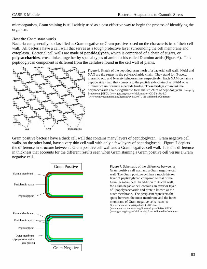
CASPiE Module Bacterial Adaptations to Osmotic Stress
83
microorganism, Gram staining is still widely used as a cost effective way to begin the process of identifying the
organism.
How the Gram stain works
Bacteria can generally be classified as Gram negative or Gram positive based on the characteristics of their cell
wall. All bacteria have a cell wall that serves as a tough protective layer surrounding the cell membrane and
cytoplasm. Bacterial cell walls are made of peptidoglycan, which is comprised of a chain of sugars, or
polysaccharides, cross-linked together by special types of amino acids called D-amino acids (Figure 6). This
peptidoglycan component is different from the cellulose found in the cell wall of plants. Figure 6. Sketch of the peptidoglycan mesh of a bacterial cell wall. NAM and
NAG are the sugars in the polysaccharide chain. They stand for N-acetyl
muramic acid and N-acetyl glucosamine, respectively. Each NAM contains a
peptide side chain that connects to the peptide side chain of an NAM on a
different chain, forming a peptide bridge. These bridges cross-link the
polysaccharide chains together to form the structure of peptidoglycan. Image by
Brudersohn [GFDL (www.gnu.org/copyleft/fdl.html) or CC-BY-SA-3.0
(www.creativecommons.org/licenses/by-sa/3.0/)], via Wikimedia Commons
Gram positive bacteria have a thick cell wall that contains many layers of peptidoglycan. Gram negative cell
walls, on the other hand, have a very thin cell wall with only a few layers of peptidoglycan. Figure 7 depicts
the difference in structure between a Gram positive cell wall and a Gram negative cell wall. It is this difference
in thickness that accounts for the different results seen when Gram staining a Gram positive cell versus a Gram
negative cell.
Figure 7. Schematic of the difference between a
Gram positive cell wall and a Gram negative cell
wall. The Gram positive cell has a much thicker
layer of peptidoglycan compared to that of the
Gram negative cell. In addition to its cell wall,
the Gram negative cell contains an exterior layer
of lipopolysaccharide and protein known as the
outer membrane. The periplasm represents the
space between the outer membrane and the inner
membrane of Gram negative cells. Image by
Graevemoore at en.wikipedia [CC-BY-SA-3.0
(www.creativecommons.org/licenses/by-sa/3.0) or GFDL
(www.gnu.org/copyleft/fdl.html)], from Wikimedia Commons

CASPiE Module Bacterial Adaptations to Osmotic Stress
84
Gram Stain Procedure
The Gram stain contains five basic steps outlined below. A schematic of how Gram positive and Gram negative
cells should appear after each step is shown in Figure 8.
1. Fixation – This first step involves heat fixing a preparation of bacterial cells known as a smear to the slide so that
they adhere strongly and are not washed off during the staining process
2. Primary stain – The primary stain crystal violet is added to heat fixed cells. Crystal violet is a positively charged
dye whose ions penetrate through the cell wall and cell membrane of both Gram positive and Gram negative cells
where they interact with negatively charged cell components and stain the cells purple.
3. Iodine treatment – After the primary stain, the now purple fixed cells are treated with iodine, which is often
referred to as a mordant. Iodine interacts with the crystal violet ions to form large complexes that are essentially
trapped inside the cell and will not easily leak out through the cell wall. This ensures that all cells remain purple.
4. Decolorization – The most important step of the Gram stain is the decolorization step. A decolorizer such as
ethanol is added to the cells. This results in a loss of crystal violet ions from Gram negative and Gram positive
cells. However, if the decolorization is done for the correct amount of time, only Gram negative cells will lose
the crystal violet ions. Since Gram negative cells have much thinner cell walls, it is easier for the crystal violet
ions to leak out of the cell. Gram positive cells are able to retain the crystal violet in their thicker cell walls that
do not leak ions as easily. If done correctly, Gram negative cells will be colorless after this step while Gram
positive cells will remain purple.
5. Counter stain – The final step is to counter stain the cells with safranin. Safranin is another positively charged
dye that stains cells in the same way as crystal violet. The addition of safranin stains all Gram negative cells that
were decolorized in the previous step. Cells that are still stained with crystal violet will not be stained with
safranin as both dyes are positively charged. After this step, Gram positive cells are purple while Gram negative
cells are pink. This color difference is how cells are differentiated.
Figure. 8. Depiction of the appearance of Gram positive and Gram
negative cells after each step of the Gram stain. White cells are considered
colorless.
2. Pre-laboratory activities
● Read the introduction and the procedures for Laboratory Period 7 in this section of the lab manual.
● Where indicated in the procedures sections in bold, work out calculations for any solutions to be made or
diluted and answer any questions posed.
● Before the lab period log onto Blackboard and take the pre-lab quiz for this week.

CASPiE Module Bacterial Adaptations to Osmotic Stress
85
3. Materials
Transduction
Equipment and materials
● Autoclaved microcentrifuge tubes
●Small tube racks
●Autoclaved pipette tips (yellow)
●P200 micropipetter
●Hockey stick
●Autoclaved toothpicks
●Jar of ethanol
●Bunsen burner
●Striker
●Sharpie
●gloves
●Pipette tip waste containers
●Toothpick waste container
●Template grid
●table top centrifuges
●vortexers
●37 degree incubator
Reagents
●Overnight cultures of F1s + P22 and recipient strain (TL 4513)
●chloroform
●LB plates + tetracycline (Tet)
●F1 pinwheel streak plate
Gram stain
Equipment and materials
●Inoculation loop
●bunsen burner
●striker ●glass slides
●microscopes
●glass marking pencil
●gloves
●paper towels
Reagents
●Overnight cultures of bacteria in LB broth
● crystal violet
●iodine
●squirt bottle of deionized H2O
●squirt bottle of 95% ethanol
●safranin

CASPiE Module Bacterial Adaptations to Osmotic Stress
86
4. Procedures Part 1: Transduction – Each person does their own cultures
REMEMBER TO PRACTICE APPROPRIATE ASEPTIC TECHNIQUE WHEN POSSIBLE!
On Monday you should have started an overnight culture of each of your ten mutants in LB. These were
inoculated into P22 buffer for you on Tuesday. Today, you will be given the mix of phage and cells. You will
kill the cells with chloroform and isolate the phage that contains pieces of the mutant DNA in their phage heads.
1. Obtain the ten overnight cultures of your mutants grown in P22 buffer.
2. Carefully pour out ten microcentrifuge tubes onto the sterile foil used to cover the beaker and place
them in a microcentrifuge rack. Put the cover back over the beaker so that the tubes remain sterile.
3. Label the tubes with your initials and M1 - M10 to correspond with your mutants.
4. Transfer 1 mL of your overnight mutant cultures in P22 buffer (labeled M1 – M10) into their
appropriate sterile microcentrifuge tubes.
5. Go to the hood and dispense 50μl of chloroform into each tube. DO NOT FLAME THE BOTTLE
6. Vortex each tube vigorously for at least 30 seconds.
7. Centrifuge your tubes at top speed for 15 minutes. Wait until the centrifuge is full before you begin
centrifuging. We will set it to spinning for you.
8. While your tubes are centrifuging, obtain ten more sterile microcentrifuge tubes and label them
with your initials and T1-T10. These are the tubes you will do the transduction in.
9. Using aseptic technique dispense 100μl of the recipient strain TL 4513 provided into each of the
ten microcentrifuge tubes.
10. After your P22 lysate tubes are done centrifuging, the supernatant is the lysate we will use for the
transduction. We do NOT want to use the pellet. Take a look at the bottom of your tubes to make
sure the pellet is remaining firmly at the bottom. Be sure you do not bump your tubes too much at
this time.
11. Using aseptic technique carefully pipet 100μl of the supernatant from tube M1 into tube T1.
Repeat this for tubes M2 and T2, M3 and T3, etc.
12. Once you have added the supernatant to all of your tubes, take the rack to the 37 degree incubator
and keep them there for 60 minutes.
13. While your transduction tubes are incubating, obtain 11 LB tetracycline plates.
14. Label 10 of these plates with your mutants, numbers 1 – 10 as well as everything else we normally
use to label plates.
15. One plate will serve as the control plate.
16. Using a grid template, map out where you will streak a small sample of your ten lysates, your ten
mutants, and your original mutagenesis strain. Which of these serve as negative controls? Which
of these are positive controls?
17. Using a sterile toothpick, pick up a small amount of the supernatant of lysate #1 and streak it on the
appropriate grid on the plate. Repeat this for lysates 2 – 10.
18. Repeat step 17, this time using the toothpick to pick up a single colony of each mutant from your
pinwheel plate.
19. Repeat step 18, using a toothpick to pick up a single colony from your original mutagenesis strain.
20. After 60 minutes, aseptically spread plate 100μl of each of your ten transductants onto the
appropriately labeled plates.
CASPiE Module Bacterial Adaptations to Osmotic Stress
87
21. Incubate all plates at 37 degrees C.
22. You will need to come back before next week to make observations and to pinwheel streak
your transductants onto LB tet plates. For each transductant plate you have spread (10
total), you will need to pinwheel streak 5 mutants onto a fresh LB Tet plate (2
transductants/plate). This can be done any time after your transductants have grown up, but
before Tuesday, 3/8.
**Please contact us if you cannot come in to remove these pinwheel streak plates from the
incubator within 24-48 hrs, so we can take them out before they overgrow.
Part 2: Gram stain
REMEMBER TO PRACTICE APPROPRIATE ASEPTIC TECHNIQUE!
1. Obtain a clean slide. Use a glass marking pencil to place an X on the side of the slide you are staining
and a circle in the middle of the slide where you will stain.
2. If you are using a broth culture, aseptically transfer a drop of culture to the slide inside the circle.
Spread evenly around the circle to make a smear. If you are using a culture from a plate, place a drop of
water inside the circle first and then aseptically use your inoculating loop to pick up a very small amount
of a colony and add that to the drop of water. Spread evenly to make a smear.
3. Allow the slide to air dry until no standing liquid is visible.
4. Heat fix the slide by passing quickly through the flame 8-10 times. Make sure to pass the slide through
the flame. Do not overheat the slide or the cell walls will be damaged and will not stain properly.
5. If you do not want to stain your hands, you may want to grab a pair of gloves to wear at this point.
6. Hold the slide straight up or set it on a flat surface over the sink. Place enough crystal violet on the slide
to cover the smear. You should not need more than several drops. Let stand 30 seconds.
7. Rinse crystal violet off with water, making sure to hold the slide at a 45 degree angle and to not squirt
the water directly on the smear.
8. Add iodine to cover the smear. Let stand 60 seconds.
9. Drain the iodine by tipping the slide over and shaking the iodine off into the sink.
10. Hold the slide at a 45 degree angle and slowly rinse with ethanol until the alcohol running off the slide
just starts to runs clear. Do not drop the alcohol directly on the smear.
11. Quickly rinse the slide with tap water.
12. Add safranin to cover the smear. Let stand 30 seconds.
13. Rinse safranin off with water.
14. Place slide between two layers of paper towel and gently blot dry.
15. Examine the slide under the microscope, describing the Gram reaction, shape, and arrangement of what
you see.
5. Post-laboratory analysis and results
We will pull your plates from the incubator this week. Sometime after Thursday, you will need to come in to
lab to make observations in your lab notebook about your transduction plates and the mini streak control plate.
Before Tuesday, you will need to pinwheel streak 5 colonies from each of your transduction plates onto fresh
LB-tet plates to create stocks of these bacteria. Colonies from 2 transductants can be streaked onto the same
LB-tet plate (keep good records of what you streak!!).
6. Preparation for the Next Laboratory Activity
● You should read the introduction and procedures before going to your next laboratory period.
● Perform any calculations in your lab notebook as indicated in the procedures portion of Laboratory 8
● Take the online pre-lab quiz

CASPiE Module Bacterial Adaptations to Osmotic Stress
88
IX. Laboratory Period 8 – Screening transductants for successful transduction of proP
gene and growth in original mutagenesis conditions
Objectives
At the end of this laboratory period the students will be able to:
1. Better understand the concept of genetic linkage
2. Describe the usefulness of antibiotic resistance in mapping regions of genetic alterations
3. Identify mutants that likely have a mutation in proP
1. Introduction
Genetic Mapping and Linkage
As you have been learning, being able to track changes in specific regions of the genome using some observable
phenotype is invaluable to our work. Tetracycline resistance (TetR) has allowed us to track the specific bacteria
that were transduced with our desired region of the genome from our donor mutant bacterium (melA gene with a
TetR cassette disruption). Recall that the melA gene is physically close to the proP gene (Figure 1).
Figure 1 – Schematic of the Salmonella typhimurium LT2 chromosome extending from bases 4,530,970 to 4,543,753
(http://blast.ncbi.nlm.nih.gov/Blast.cgi). This region contains the proP gene and the melA gene as well as the region in between, which contains 7
additional genes whose coding region is on the opposite strand, as indicated by the arrows. The P22 bacteriophage is capable of fitting 44,000
basepairs of DNA in its head, and the total distance between the proP and melA genes is 12,783 basepairs. This distance is large enough that some
phage will not be able to pick up both genes and the distance between them but also small enough so that some phage will.
The ability of the transduced (F1T ) bacteria to grow in the presence of tetracycline tells us that a piece of the
genome close to where the proP gene is was transferred to our recipient strain. However, we don’t know for
sure whether the proP gene was also co-transduced (Figure 2). Our recipient bacteria strain had another
antibiotic resistance present (Chloramphenicol resistance (CamR)) which was inserted into the proP gene,
making the proP gene non-functional, but giving the bacteria the ability to grow in the presence of
chloramphenicol. To distinguish between our two possibilities (tetracycline resistance tranduced with or
without the proP gene), we can screen our transductants for the ability to grow in the presence of
chloramphenicol. Transductants that had the mutant proP gene co-transduced should not be able to grow on
these plates and transductants that did not will still have the CamR cassette present in the recipient strain and
will be able to grow on these plates.
melA proP
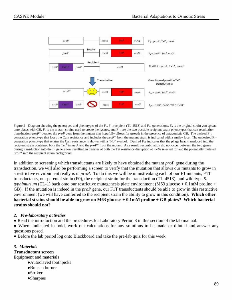
CASPiE Module Bacterial Adaptations to Osmotic Stress
89
Figure 2 - Diagram showing the genotypes and phenotypes of the F0, F1, recipient (TL 4513) and F1T generations. F0 is the original strain you spread
onto plates with GB, F1 is the mutant strains used to create the lysates, and F1T are the two possible recipient strain phenotypes that can result after
transduction. proP* denotes the proP gene from the mutant that hopefully allows for growth in the presence of antagonistic GB. The desired F1T
generation phenotype that loses the Cam resistance and includes the proP* from the mutant strain is indicated with a smiley face. The undesired F1T
generation phenotype that retains the Cam resistance is shown with a “No” symbol. Desired F1T indicates that the phage head transduced into the
recipient strain contained both the TetR in melA and the proP* from the mutant. As a result, recombination did not occur between the two genes
during transduction into the F1 generation, resulting in transfer of both the Tet resistance disruption of melA selected for and the potentially mutated
proP* into the recipient strain background.
In addition to screening which transductants are likely to have obtained the mutant proP gene during the
transduction, we will also be performing a screen to verify that the mutation that allows our mutants to grow in
a restrictive environment really is in proP. To do this we will be ministreaking each of our F1 mutants, F1T
transductants, our parental strain (F0), the recipient strain for the transduction (TL-4513), and wild type S.
typhimurium (TL-1) back onto our restrictive mutagenesis plate environment (M63 glucose + 0.1mM proline +
GB). If the mutation is indeed in the proP gene, our F1T transductants should be able to grow in this restrictive
environment (we will have conferred to the recipient strain the ability to grow in this condition). Which other
bacterial strains should be able to grow on M63 glucose + 0.1mM proline + GB plates? Which bacterial
strains should not?
2. Pre-laboratory activities
● Read the introduction and the procedures for Laboratory Period 8 in this section of the lab manual.
● Where indicated in bold, work out calculations for any solutions to be made or diluted and answer any
questions posed.
● Before the lab period log onto Blackboard and take the pre-lab quiz for this week.
3. Materials
Transductant screen
Equipment and materials
●Autoclaved toothpicks
●Bunsen burner
●Striker
●Sharpies
CASPiE Module Bacterial Adaptations to Osmotic Stress
90
●p200 micropipetters
●Sterile p200 tips
●Pipette tip waste containers
●Toothpick waste container
●37 degree incubator
●Template grid (100 grid)
●Ministreak data sheet
Reagents
● Pinwheel streaked plates of F0 bacteria (TL-1673, dinB-, uvrD
-, or mutS
-)
● Pinwheel streaked plates of F1 mutants
●Pinwheel streaked plates of F1T transductants
●Pinwheel streaked plates of TL-1
●Pinwheel streaked plates of TL-4513
●M63 glucose plates
●M63 glucose + 0.1mM pro plates
●M63 glucose + 0.1 mM pro and 2mM GB plates
●LB + Tet plates
●LB + Cam plates
●Sterile 1 M GB stock solution
4. Procedures Part 1: Screening of F1T transductants on LB-Cam and original mutagenesis media
REMEMBER TO PRACTICE APPROPRIATE ASEPTIC TECHNIQUE!
1. Each person needs one each of the following plates: (1) M63 glucose + pro, (2) M63 glucose + 0.1mM
pro + 2 mM GB, (3) M63 glucose, (4) LB + cam, and (5) LB + tet.
2. Label each type of plate you will mini streak each of your F0 strain, F1 mutants, F1T transductants, TL-1,
TL-4513 with your initials, the date, and the media. (note in your lab notebook all of the strains...not on
the plate this time!). Also make a reference line at the top of the plate to assist in orienting the grid
under the plate
3. If your mutagenesis conditions had a GB concentration greater than 2mM you need to supplement the
M63 glucose + 0.1mM proline + 2 mM GB media with more GB to increase its concentration above
2mM. Do that now and set the plates aside to dry.
4. Obtain a 100 grid template and use the data sheet that we provide to make a key for your plating (you
will keep a copy in your lab notebook and leave a copy in the lab for us).
*in naming your F1T transductants, remember that the bacteria in each of your 5 pinwheel streak sections of
transductants came from the same F1 mutant. They just differ in which part of the F1 genome they have, but
any change in proP would be identical.
A good naming scheme would be:
F1T(x,y)
Where: F1T is the generation name, x refers to the transductant number (and mutant number) and y refers to the
colony taken from the transduction plate (and pinwheel streak section #). If all 10 of your transductions
produced growth of at least 5 colonies, x would vary from 1-10 and y would vary from 1-5.

CASPiE Module Bacterial Adaptations to Osmotic Stress
91
5. Line up the M63 plates in this order: M63 glucose + pro and GB, M63 glucose, and M63 glucose +pro.
Why do you want to streak them in this order? What is the purpose of the M63 glucose plate?
What is the purpose of the M63 glucose + proline plate? Why are we plating the transduction
recipient strain on these plates?
6. Using aseptic technique, use an autoclaved toothpick to streak a single colony from your pinwheel streak
plate onto the appropriate section in the grid on each plate in the order in #4 (use the same toothpick and
colony across all three plates).
7. Repeat this for all the pinwheel streaked F1T transductants, F1 mutants, F0 strain, TL-4513, and TL-1.
Why are we streaking TL-1 onto the M63 glucose plate?
8. Repeat steps 6 and 7 with a different colony from each pinwheel streaked plate of each strain on an LB +
cam and LB + Tet plate. Why are repeating the plating onto LB + Tet plates?
9. Invert the plates and incubate at 37 degrees C.
5. Post-laboratory analysis and results
We will remove your plates from the incubator and put them in the middle refrigerator in the lab, but you need
to come in before the next lab to make observations in your lab notebook.
6. Preparation for the Next Laboratory Activity
● You should read the introduction and procedures before going to your next laboratory period.
● Perform any calculations in your lab notebook as indicated in the procedures portion of Laboratory 9
● Take the online pre-lab quiz

CASPiE Module Bacterial Adaptations to Osmotic Stress
92
X. Laboratory Period 9 –Functional testing of mutants, presenting data in poster
format
Objectives
At the end of this laboratory period the students will be able to:
1. Design and perform experiments to better define mutant phenotypes
3. Measure growth rates of proP mutants
4. Describe the basic components of a research poster
5. Appreciate the differences between research posters and research papers
1. Introduction
A. Introduction for parts 1 of the procedures
GB antagonism effectiveness, proline transport plate assay, and growth curves
Now that you have mapped the mutation of some members of your F1 generation to the proP gene, we can
perform some basic experiments to see what might have changed in these mutants allowing them to overcome
the GB antagonism. Specifically, we will test two things – Are these mutants able to grow at a higher relative
concentration of GB to proline? Are these mutants able to grow better in the presence of lower proline
concentrations?
To test whether or not the mutants can grow at a higher relative concentration of GB to proline, we will use
M63 glucose + proline plates onto which we have placed a sterile filter disc. We will divide the plates into four
quadrants and ministreak four strains as shown in Figure 1. Two of the strains will be our mutant F1s. What
other two strains should we streak onto these plates as controls? We will aseptically transfer gradually
increasing concentrations of GB onto the sterile discs with a micropipettor. Once the strains have grown, we
can measure how close they have grown to the disc. All strains should be able to grow on the M63 glucose +
proline plates, but the better they are able to grow in the presence of antagonistic concentrations of GB, the
closer they will grow to the disc. We will streak two samples of each strain onto the plate. Why do you think
we should do this? We will do this experiment on M63 glucose + proline + 0.3 M NaCl plates as well to see if
the phenotype is any different under osmotic stress conditions.
We will similarly test whether the mutants are able to grow better than F0 in the presence of lower proline
concentrations. For this test, we will use the same disc-plate set-up for the previous experiment, but we will be
using M63 glucose plates and we will pipet proline onto the discs instead of glycine betaine. Our F0 and F1
strains should not be able to grow unless they are supplemented with proline. If the F1 mutants are able to grow
better at lower proline concentrations than F0, it suggests the mutants have an increased affinity for proline or an
increased proline transport rate. We can measure better growth quantitatively by the distance the ministreak
extends from the disc and qualitatively by the thickness of the ministreak after a given period of time. The
further the ministreak extends from the disc, the better the strain is able to grow at lower proline concentrations.
We will repeat this experiment on M63 glucose + 0.3 M NaCl plates as well.

CASPiE Module Bacterial Adaptations to Osmotic Stress
93
Figure 1. Diagram of the plating scheme for the disc assays. The white circle in the middle represents the sterile filter disc upon which glycine
betaine or proline will be pipetted. Straight lines in the four quadrants represent the streaking pattern of the bacterial strains.
B. Introduction for Part 2 of the procedures
Performing bacterial growth curves Another functional test that we can perform to better define our mutant bacteria is to determine if the F1 mutant bacteria
grow at different rates in 0.1mM proline than the F0 strain. In lab 4 you performed bacterial growth curves and calculated
the doubling rate of mutant bacterial strains isolated by CASPiE students in the spring of 2010. Each of you will do this
for a proP mutant today in lab to better characterize the mutants that can grow in the presence of an antagonistic
concentration of GB. In lab 4, we set up the cultures and took the first, time zero, OD600 reading for you. You will be
setting up the cultures for the time zero reading yourselves today!
There are multiple steps leading up to the point where you will enter the process at the start of class and these are depicted
in Figure 2. On Monday, a tube of LB broth was inoculated with a single colony from a mutant pinwheel streak plate.
This culture was allowed to grow up overnight (ON) at 37o C on a shaker. The process starts in LB media because it is an
enriched media and the bacteria should grow up quickly and well. On Tuesday, a tube of M63 glucose + 1mM proline
broth was inoculated with some of the bacteria from the ON LB culture. This culture was allowed to grow up ON at 37o
C on a shaker. When you come in to lab on Wednesday, you will inoculate a flask of M63 glucose + 0.1mM proline broth
with an aliquot from the ON M63 glucose + 1mM proline culture and start the growth curve measurements. Note that the
concentration of proline in the M63 glucose overnight culture is higher than the concentration we have used thus far in our
experiments and will use in the growth curves (1mM compared to 0.1mM). What might be the purpose of growing the
bacteria up at a higher concentration of proline overnight before the growth curve assay?
Figure 2. Schematic of the preparation
of bacteria for growth curve analysis
F1T,1 F1T,2
? ?

CASPiE Module Bacterial Adaptations to Osmotic Stress
94
In order to make accurate measurement of the growth of the bacteria, we need to have a starting concentration of bacteria
that we can measure, but that is low enough that we will be able to capture the exponential growth of the culture using the
spectrophotometers. Therefore, we need to perform the appropriate dilution of the overnight M63 glucose + 1mM proline
culture for our time zero starting point. To do this, we need to determine the OD600 of the overnight culture to get an
estimate of the concentration of cells that we are starting with. The overnight culture has too many cells in it to measure
with the spectrophotometer, so you will have to dilute it and back calculate to get the estimated OD600 of the undiluted
culture. You will be taking 500 µL of the overnight culture and diluting it into 2.5 mL of M63 broth. What is the
dilution factor for this dilution? We can proceed with a variation on the C1V1 = C2V2 calculations that we have been
making this semester to determine the aliquot volume from the M63 glucose + 1 mM proline culture we need to use to
start our growth curve measurements. The concentration of the ON culture (C1) is the estimated OD600 of the culture
(OD600 of diluted culture * DF). Our desired final concentration for time zero in our growth curve measurements is OD600
= 0.08. The calculations that need to be done to determine the aliquot volume are depicted in Figure 3.
Figure 3. Schematic of the inoculation of 30 mL of M63
glucose + 0.1 mM proline broth with an aliquot from an ON
culture of our mutant bacteria and the calculations
involved.
C. Presenting data in poster format
You will be presenting the results from your experiments in the form of a research poster. A poster contains
many of the same components as a research paper (Title, Introduction, Methods, Results,
Discussion/Conclusions, References), but with less text. Concise, take-home messages paired with clear
graphical representations of the data to communicate with your audience are the form. Below you will find a
general description of the components of a poster. I have posted a poster of mine up on Blackboard for you to
look at to get an idea of the basic layout and style of this type of data reporting. A useful website with more
information about designing posters is: http://www.asp.org/education/howto_onPosters.html
Title
While this is the shortest piece of text on the poster, it can be the hardest to craft. You need to distill what it is
that your data mean and put it into one sentence. This sentence should give the audience the take-home
message/most important finding from your experiments.
Introduction
CASPiE Module Bacterial Adaptations to Osmotic Stress
95
The introduction is challenging to write and many people write it last after seeing how all the results turn out.
You need to have your take-home message in mind and give the appropriate background information for your
audience to best appreciate your experiments and analysis. The introduction should be 1-2 paragraphs and
contain a basic statement about your research objective, some statements to put your work into context (the
basic strategies for osmoregulation and general properties of ProP transport, for example), and statements
about your particular hypothesis and predictions. You don’t need to do an entire detailed review of your topic,
but hit on the important general aspects and those that are pertinent to your particular research question.
Please be sure that your hypothesis is explicitly stated at the end of your introduction.
Methods
As in research papers, the methods section should provide enough detail that people in your field of research
would be able to repeat your experiments. In our case, your fellow classmates are your colleagues. They
understand the basic preparation and approach, but would need the exact concentrations of drugs, types of
treatments, data analysis methods, etc., to replicate your work themselves. Having said that, I want you to
give a bit more detail to show to me that you understand what you are doing yourself.
Results
Aside from the figure title and legend, the results section of a poster has very little text. It consists of a series
of figures to take your audience through your results. In theory, the figures, with their titles and legends,
should be able to stand alone from the poster if needed. You need to carefully construct your figures so they
are clear without any accompanying text. They should be simple and readable from a distance of about 2 feet.
The figure title is similar to the poster title in that it should be a brief statement that gives the overall take-
home message from the figure. This should be in large font and be placed above the figure.
The figure legend should be a brief description of the data contained within the figure and any important
experimental/procedural details such as solution concentrations, incubations. This is the place where you
should define any symbols used in the graphs, explain color-coding, etc. Small, but readable, font should be
used and the legend should be placed under the figure.
The figure itself should be as simple as possible with axis labels and symbols large enough to be read from a
short distance. Make sure that your choice of format to represent your data illustrates your point clearly. For
example, the dependence of bacterial growth on external GB concentration is well-illustrated with a line graph
as opposed to a bar graph. However, the growth of different bacterial strains in different media types would
be suited by a bar graph. Please consult the Guide to Figures and Graphs up on Blackboard or ask if you are
unsure.
Discussion/Conclusions
This section is where you put your results back into the context you set up in the introduction and relate your
findings to your hypotheses and predictions. Bullet points are great here. You should cover the overall
finding, and then give the specific, important finding(s), and why this is important. You should give some
thoughtful statements about how your results are important for the function of the bacterium and organisms in
general.
References
Please cite any sources that were directly relevant or informative for your project. I would like you to consult
1-2 primary literature articles for this assignment. You can use APA citation formatting.

CASPiE Module Bacterial Adaptations to Osmotic Stress
96
Acknowledgements
Scientific research is at its best when there is collaboration between colleagues and peers. Please acknowledge
people that made a significant impact on your work (the experiments themselves and the contents of your
poster) with a simple sentence naming them and how they contributed to your final project!
2. Pre-laboratory activities
You need to record observations in your lab notebook on your transductant screen that you set up before
spring break.
● Read the introduction and the procedures for Laboratory Period 9 in this section of the lab manual.
● Where indicated in bold, work out calculations for any solutions to be made or diluted and answer any
questions posed.
● Before the lab period log onto Blackboard and take the pre-lab quiz for this week.
3. Materials
GB antagonism and proline uptake plate assay
Equipment and materials
●Bunsen burner
●Striker
●Sterile toothpicks
●Toothpick waste containers
●forceps
●Sterile filter paper discs
●P20 micropipette tips
●P20 micropipetters
Reagents
●control bacteria pinwheel streak plate
●F0 pinwheel streak plate
●F1T pinwheel streak plate
●Sterile 2 M GB solution
●Sterile 100 mM proline solution
●M63 glucose + 0.1 mM proline plates
●M63 glucose + 0.1 mM proline + 0.3 M NaCl plates
●M63 glucose + 0.3 M NaCl plates
●M63 glucose plates
Spectrophotometry:: Measuring bacterial growth rates
Equipment and materials
●Spectrophotometers
●Cuvettes (2/group)
●Test tube rack
●125 ml Erlenmeyer flasks
●Sharpies
●Squirt bottles of water
●Squirt bottles of 70% EtOH
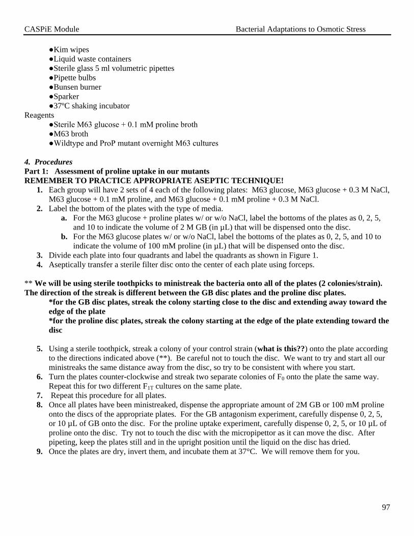
CASPiE Module Bacterial Adaptations to Osmotic Stress
97
●Kim wipes
●Liquid waste containers
●Sterile glass 5 ml volumetric pipettes
●Pipette bulbs
●Bunsen burner
●Sparker
●37ºC shaking incubator
Reagents
●Sterile M63 glucose + 0.1 mM proline broth
●M63 broth
●Wildtype and ProP mutant overnight M63 cultures
4. Procedures Part 1: Assessment of proline uptake in our mutants
REMEMBER TO PRACTICE APPROPRIATE ASEPTIC TECHNIQUE!
1. Each group will have 2 sets of 4 each of the following plates: M63 glucose, M63 glucose + 0.3 M NaCl,
M63 glucose + 0.1 mM proline, and M63 glucose + 0.1 mM proline + 0.3 M NaCl.
2. Label the bottom of the plates with the type of media.
a. For the M63 glucose + proline plates w/ or w/o NaCl, label the bottoms of the plates as 0, 2, 5,
and 10 to indicate the volume of 2 M GB (in µL) that will be dispensed onto the disc.
b. For the M63 glucose plates w/ or w/o NaCl, label the bottoms of the plates as 0, 2, 5, and 10 to
indicate the volume of 100 mM proline (in µL) that will be dispensed onto the disc.
3. Divide each plate into four quadrants and label the quadrants as shown in Figure 1.
4. Aseptically transfer a sterile filter disc onto the center of each plate using forceps.
** We will be using sterile toothpicks to ministreak the bacteria onto all of the plates (2 colonies/strain).
The direction of the streak is different between the GB disc plates and the proline disc plates.
*for the GB disc plates, streak the colony starting close to the disc and extending away toward the
edge of the plate
*for the proline disc plates, streak the colony starting at the edge of the plate extending toward the
disc
5. Using a sterile toothpick, streak a colony of your control strain (what is this??) onto the plate according
to the directions indicated above (**). Be careful not to touch the disc. We want to try and start all our
ministreaks the same distance away from the disc, so try to be consistent with where you start.
6. Turn the plates counter-clockwise and streak two separate colonies of F0 onto the plate the same way.
Repeat this for two different F1T cultures on the same plate.
7. Repeat this procedure for all plates.
8. Once all plates have been ministreaked, dispense the appropriate amount of 2M GB or 100 mM proline
onto the discs of the appropriate plates. For the GB antagonism experiment, carefully dispense 0, 2, 5,
or 10 µL of GB onto the disc. For the proline uptake experiment, carefully dispense 0, 2, 5, or 10 µL of
proline onto the disc. Try not to touch the disc with the micropipettor as it can move the disc. After
pipeting, keep the plates still and in the upright position until the liquid on the disc has dried.
9. Once the plates are dry, invert them, and incubate them at 37°C. We will remove them for you.

CASPiE Module Bacterial Adaptations to Osmotic Stress
98
Part 2: Bacterial growth curves: Doubling time of F1 mutants
REMEMBER TO PRACTICE APPROPRIATE ASEPTIC TECHNIQUE!
Refer to your notes and Lab 4 about the basics of making measurements of bacterial growth curves.
At the start of the lab there will be a bottleneck at the specs, so you should feel free to come in early to
measure the OD600 of your ON culture to determine the volume of the aliquot you need to use to inoculate
your M63 glucose + 0.1mM proline broth with to do your time zero measurement.
1. Obtain a clean cuvette and perform a dilution of your ON bacterial culture by aseptically pipeting 500
µL of culture into 2.5 mL of M63 broth.
2. Blank the spectrophotometer and measure the absorbance of the diluted culture at 600 nm.
3. Use this absorbance to determine the aliquot you need to use from your overnight culture (see Figure 3).
Check your calculations with us before you do the inoculation.
5. Post-laboratory analysis and results
● You need to come in and make observations in your lab notebook about your GB antagonism and
proline uptake plates before next week. You should also calculate the doubling time of your mutants
from the growth curves in liquid culture.
6. Preparation for the Next Laboratory Activity
● You should read the introduction and procedures before going to your next laboratory period.
● Perform any calculations and answer any questions in your lab notebook as indicated in the manual
for Laboratory 10.
● Take the online pre-lab quiz

CASPiE Module Bacterial Adaptations to Osmotic Stress
99
XI. Laboratory Period 10 – Preparation for PCR amplification of the proP gene
Objectives
At the end of this laboratory period the students will be able to:
1. Explain a PCR amplification of a gene
2. Fill wells in an agarose gel
3. Organize, prepare and present preliminary data to the class
1. Introduction
A. Introduction for the procedures for lab April 6th
PCR amplification of the proP gene (written in consultation with Cell and Molecular Biology: Concepts and Experiments, 4th
Edition, Gerald Karp)
In class on April 6th we will be isolating the DNA from our F1Ts that have passed through our functional
mapping, suggesting that they have a mutation in the proP gene and make many copies (amplification) of the
gene to be sent for sequencing to determine the identity of the mutation in the gene! While DNA extraction
from the nuclei of eukaryotic cells involves many steps, we can simply use the heat from the DNA
amplification process to lyse our cells, thereby liberating their chromosome. To amplify the proP gene from
our F1 mutants, we will be using PCR (polymerase chain reaction). PCR is the process by which a single
copy of DNA can be exponentially amplified very quickly. It was developed in 1983 by Kary Mullins and has
become an indispensible technique to scientists from diverse disciplines, from ecologists to biochemists to
budding bacterial geneticists!
PCR basically involves multiple cycles of replication that can yield billions of DNA copies from a single
starting copy in just a few hours. The DNA of interest is mixed together with: DNA polymerase,
deoxynucleotides (dATP, dGTP, dCTP, dTTP), and primers. The DNA polymerase that is used is a heat-stable
polymerase, Taq polymerase, that was originally isolated from a thermal springs (temperatures >90 degrees C)
bacterium called Thermus aquaticus. The importance of this thermal stability will become clear below. The
primers are short synthetic pieces of DNA (oligonucleotides) that are designed to be complementary to DNA
sequences at the 3’ ends of the regions of the DNA just upstream of the promoter and just downstream of the
protein coding region of the gene of interest (for a schematic of this, see
http://bioweb.uwlax.edu/genweb/molecular/seq_anal/primer_design/primer_design.htm). These serve as
specific starting places along the whole chromosome for the Taq polymerase to add nucleotides.
The process of PCR gene amplification is shown in Figure 1 and consists of three steps: (1) Denaturation of
double stranded DNA , (2) Annealing of the primers to the DNA, and (3) Extension from the primers. To
initiate replication of the gene of interest, the sample with the DNA, primers, deoxynucleotides, and Taq
polymerase is heated to a temperature that is high enough to separate the two complementary strands of DNA
from one another (denature/melt) without damaging them (~ 94 degrees C). The temperature is then shifted to a
temperature that allows the primers to bind (anneal) to the DNA strands (~52 degrees C, for us). The
temperature is then raised to a level that is conducive for the Taq polymerase to add deoxynucleotides extending
from the primers (~ 72 degrees C). This extension selectively makes copies of the DNA region of interest

CASPiE Module Bacterial Adaptations to Osmotic Stress
100
(proP gene, in our case) forming new complementary strands. One cycle of amplification is now complete,
yielding two copies of the gene of interest from each original one present in our sample (one/bacterium)!
Figure 1. Schematic of the general process of PCR amplification of a DNA
region of interest. The three steps of denaturation, annealing, and extension
are depicted. Image by Tinojasontran (Own work) [Public domain], via
Wikimedia Commons.
The whole process of complementary strand separation, primer binding and elongation, and annealing is
repeated 30-35 times, each time doubling the amount of the gene of interest (Figure 2). The PCR machine that
we will use is called a thermal cycler because it can be programmed to cycle between the three temperatures
that we need over and over again. We will be taking the DNA from a single colony (~ 109 cells) and taking it
through 30 cycles to amplify the proP gene.
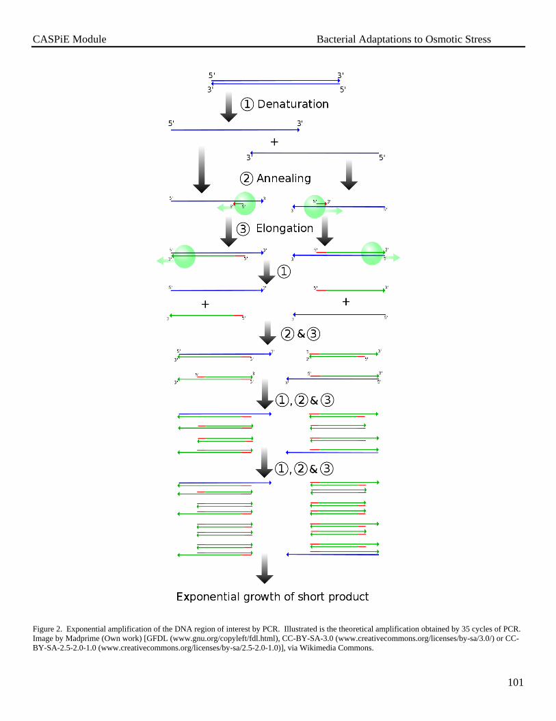
CASPiE Module Bacterial Adaptations to Osmotic Stress
101
Figure 2. Exponential amplification of the DNA region of interest by PCR. Illustrated is the theoretical amplification obtained by 35 cycles of PCR.
Image by Madprime (Own work) [GFDL (www.gnu.org/copyleft/fdl.html), CC-BY-SA-3.0 (www.creativecommons.org/licenses/by-sa/3.0/) or CC-
BY-SA-2.5-2.0-1.0 (www.creativecommons.org/licenses/by-sa/2.5-2.0-1.0)], via Wikimedia Commons.

CASPiE Module Bacterial Adaptations to Osmotic Stress
102
Agarose gel electrophoresis of the PCR product
Before we can send over our samples for DNA sequencing we need to verify a number of things. The first thing
that we need to verify is that we have a PCR product in the first place! Secondly, we need to verify that this
product is likely our gene of interest. Lastly, we need to verify that we have amplified only our gene of interest
and nothing else. To do this, we will use a technique called agarose gel electrophoresis.
Agarose gels are useful for separating charged molecules from each other based on their size because it
provides an electrically-neutral matrix through which things can move. A schematic for this process can be
found at: http://www.molecularstation.com/molecular-biology-techniques/gel-electrophoresis/. The agarose is
covered with a buffered solution and samples of DNA are loaded into wells in the agarose. An electric field is
applied across the gel with a voltage source such that the negative pole is located near the loaded samples and
the positive pole is located on the opposite end of the gel. Negatively-charged DNA or pieces of it will then
migrate toward the positive pole at a rate that is inversely proportional to their size. Smaller pieces of DNA will
migrate faster and further along the gel than larger pieces. A sample filled with molecules of known sizes is
loaded onto the same gel as experimental samples to provide size points of reference to compare experimental
samples to. This sample is known as a ladder because of the pattern on the gel that it creates (lanes 1 and 8 in
Figure 3).
The samples of DNA can be visualized within the gel by including the UV-activated DNA intercalating agent,
ethidium bromide (EtBr) within the agarose gel or applying it after the samples have migrated. EtBr inserts
itself into the DNA and fluoresces when exposed to UV light. An example of an agarose gel with DNA
samples loaded onto it is shown in Figure 3. This is a nice example showing six successful PCR reactions in
lanes 2-6. We are hoping for a result similar to this with a single band at 2 kb size for the proP gene. Figure 3
also shows a picture of the gel with the PCR-amplified proP gene from the mutants isolated by CASPiE
students in the Spring of 2010!

CASPiE Module Bacterial Adaptations to Osmotic Stress
103
Figure 3. Top: Sample agarose gel with PCR products visualized by EtBr fluorescence. Image from: DNA Agarose Gel Electrophor.jpg From
English Wikipedia: http://en.wikipedia.org/wiki/Image:DNA_Agarose_Gel_Electrophor.jpg {{GFDL}} Bottom: Gel with mutant proP PCR
products from the Spring of 2010.
To prepare for the PCR next week we will choose the mutants we wish to sequence the proP gene from and
practice loading samples into wells in agarose gels.
2. Pre-laboratory activities
You need to come into the lab before Wednesday and make observations and measurements from your
radial streak functional assay plates. In addition, you need to calculate the doubling time of your mutant
bacteria growth curves. We will check your lab notebooks at the start of the class.
● Read the introduction for Laboratory Period 10 in this section of the lab manual.
● Before the lab period log onto Blackboard and take the pre-lab quiz for this week.

CASPiE Module Bacterial Adaptations to Osmotic Stress
104
3. Materials
Practice filling wells in an agarose gel
Equipment and materials
● p20 micropipetter
● p20 pipet tips
● agarose-filled petri dishes with wells
Reagents
● loading buffer
4. Procedures Part 1: Practice filling wells in an agarose gel
We will demonstrate this for you in class.
5. Post-laboratory analysis and results
● Write a draft of a concise methods for the mutagenesis, transduction, and functional screens for your
poster.
6. Preparation for the Next Laboratory Activity
● You should read the introduction and procedures before going to your next laboratory period.
● Perform any calculations and answer any questions in your lab notebook as indicated in the manual
for Laboratory 11.
● Take the online pre-lab quiz

CASPiE Module Bacterial Adaptations to Osmotic Stress
105
XII. Laboratory Period 11 – PCR amplification of the proP gene and practicing
sequencing proP gene
Objectives
At the end of this laboratory period the students will be able to:
4. Explain a PCR amplification of a gene
5. Perform a PCR
6. Make an agarose gel
7. Interpret an agarose DNA gel
8. Use BLAST to sequence the proP gene
1. Introduction
A. Introduction for parts 1 & 2 of the procedures
PCR amplification of the proP gene (written in consultation with Cell and Molecular Biology: Concepts and Experiments, 4th
Edition, Gerald Karp)
Please review the background information on PCR and gel electrophoresis from last week’s lab manual.
B. Introduction for part 3 of the procedures
Bioinformatics: Practice sequencing the proP gene
Dr. Csonka has written a nice guide to assist you with this for this week and next week. You need to download
the file from Blackboard and read over it before lab this week (it’s in the Lab 11 folder, “Bioinformatics Info”).
Bring a copy of it with you to lab on Wednesday to help you work on analyzing DNA sequences.
C. Transport across biological membranes:: Quantitative look at carrier mediated transport
Facilitated diffusion of substances across the plasma membrane via carrier-mediated transport involves an
integral membrane protein that transports solutes across the membrane according to gradients for that solute. A
hallmark feature of this type of transport is that it can be saturated. What this means is that transport of solutes
will increase with increasing concentrations of the solutes until all of the transporters are occupied with solute
and a maximum transport rate is reached (Figure 1). At this point, the transport rate, or velocity, becomes
constant and will not increase with further increases in solute concentrations. This saturation is a function of
the fact that the transported substance needs to bind to the transporter and then the transport protein must
change its conformation in order to move the substance across the membrane. This takes time and limits the
availability of the transporters to move solutes. In contrast, once an ion channel is opened (gated) substances
can more or less freely diffuse through it according to their gradients via simple diffusion. A schematic of this
can be seen at: http://www.biochem.arizona.edu/classes/bioc462/462a/NOTES/LIPIDS/transport.html.
Figure 1. Schematic illustrating the differences between passive,
simple diffusion and facilitated diffusion.

CASPiE Module Bacterial Adaptations to Osmotic Stress
106
The basics of enzyme kinetics, as originally described in 1913 by Leonor Michaelis and Maud Menten, can
be applied to facilitated diffusion. The binding and transport of a solute can be likened to binding of a substrate
with the enzyme and the ensuing reaction. In both enzymatic reactions and substrate transport there is (1)
binding of the substrate/solute to the enzyme/carrier protein and (2) a reaction that changes the substrate or
position of the substrate (for transport). The mathematical description of this basic process is:
V = Vmax [S]____
[S] + KM
Where:
V is the velocity of the reaction (= transport rate)
Vmax is the maximum velocity at the saturation point (= maximum transport rate)
[S] is the concentration of the substrate or solute
KM is the Michaelis constant. The KM is the substrate/solute concentration when the reaction or transport
velocity is ½ maximum (Vmax)
The most useful parameters from the above Michaelis-Menten equation for evaluating the functioning of
transporters are the Vmax and KM. Changes in transporter Vmax will provide global information about the
functioning or number of the transporters in moving substances or efficacy of noncompetitive inhibitors of
transport (Figure 2). Increases in Vmax could result from an increase in transporter number or changes in the
way the transporter operates. Changes in KM will reflect the affinity of the solute for the transporter and the
rates of its subsequent transport across the membrane. It can also provide information about the effectiveness of
competitive inhibitors of transport (Figure 2). An increase in KM means that the apparent affinity has been
reduced and a higher concentration of solute is needed to reach ½ Vmax for transport. Measurements of the KM
are can be done by performing transport assays to determine V at various solute concentrations ([S]) and then
estimating Vmax and KM from those data from the Michaelis-Menten plot.
Figure 2. Example plots showing the changes in the Vmax and KM with competitive (top) and noncompetitive (bottom) inhibition. Inhibition plots
are shown in blue and labeled with a “2”. Note that competitive inhibitors do not change the Vmax, but a high [S] is needed to reach it (altered KM).
In contrast, noncompetitive antagonists decrease the Vmax. Images by Sponk (Own work) [Public domain or Public domain], via Wikimedia
Commons.

CASPiE Module Bacterial Adaptations to Osmotic Stress
107
A more accurate way to estimate Vmax and KM is to linearize the relationship between V and [S] by plotting the
reciprocal of the velocities of transport as a function of the reciprocal of [S]. This results in a line with a slope
of KM/Vmax whose y-intercept is 1/Vmax and the x-intercept is -1/KM (Figure 3). This linear plot is also know as
a Lineweaver-Burk plot.
Figure 3. Example of a Lineweaver-Burk plot. Image by Pro bug catcher at the English language Wikipedia [GFDL
(www.gnu.org/copyleft/fdl.html) or CC-BY-SA-3.0 (www.creativecommons.org/licenses/by-sa/3.0/)], from Wikimedia Commons.
There are other derivations from the Michaelis-Menten description that are used to describe enzymes and
transporters. An example of this is used in one of our papers (Botfield and Wilson, 1988), the Eadie-Hofstee
plot which was used to estimate KM and Vmax, by plotting V as a function of V/[S], but has since been replaced
by linear regression. In this linearization of the Michaelis-Menten plot the y-intercept is the Vmax and the slope
is –KM. One limitation to this is that both variables plotted are dependent variables.
The ProP transporter falls under the category of secondary active transport and uses the energy stored in the
proton (H+) electrochemical gradient to move compatible solutes, such as proline and glycine betaine, across the
membrane along with the proton down its gradient. ProP is an example of a symporter which means that the
protons and solutes are transported in the same direction. In most instances there is a proton gradient to enter
the cell which then allows for the movement of proline/glycine betaine into the cell. Assuming that the
concentrations of protons and proline/glycine betaine are in equal proportion to one another, the behavior of
transport can be described as above.
D. The proposed structure and functioning of the ProP transporter (written in consultation with Culham, D.E. et al., 2008.
Periplasmic loops of osmosensory transporter Prop in Escherichia coli are sensitive to osmolality. Biochemistry. 47:13584-13593 and Wood, J.M. et
al., 2005. A structural model for the osmosensor, transporter, and osmoregulatory ProP of Escherichia coli. Biochemistry. 44:5634-5646.)
ProP, as you know, is a 500 amino acid integral membrane protein that acts as a H+-osmoprotectant symporter
for proline and glycine betaine. It is able to sense osmotic stress in the environment and increase its transport
rate in response. A diagram of the ProP structure is shown in Figures 4 and 5. ProP is a member of the major
facilitator superfamily (MFS) of proteins that contains 12 alpha helical transmembrane domains, regions of the
protein that pass through the inner membrane separating the cytoplasm and the periplasm. It also contains a
cytoplasmic N-terminal domain found near the beginning of the protein and a cytoplasmic C-terminal domain
found at the end of the protein, often referred to as a coiled-coil domain due to the secondary structure it adopts.

CASPiE Module Bacterial Adaptations to Osmotic Stress
108
N-terminal refers to the amino group of the first amino acid in the protein sequence, and C-terminal refers to the
carboxyl group of the last amino acid in the protein sequence. The twelve intermembrane regions are connected
by periplasmic and cytoplasmic loops. The intermembrane regions are hydrophobic while the N-terminus, C-
terminus, and loops found in both the periplasm and cytoplasm are hydrophilic.
When the protein folds together to form a transporter in the membrane, it is believed that transmembrane
regions I, IV, VII, and X contact each other to line an inner pore that is also partly surrounded by regions II, V,
VIII, and XI. Transmembrane regions III, VI, IX, and XII are on the exterior facing the surrounding membrane.
Regions II and XI are believed to make contact as are regions V and VIII. There are conserved ionizable amino
acids among ProP sequences of related organisms in regions I, II, and IV-VI, indicating that these amino acids
may be involved in transport of H+
or proline/glycine betaine. We will be constructing our own 3-dimensional
model of ProP next week to get a better feel for how the protein is thought to be structured.
The coiled coil domain at the C-terminus has been shown to modulate the threshold for osmotic activation, but
it does not act as an actual osmosensor. In other words, mutations to or deletions of the coiled coil alter the
level of osmotic stress that must be present in order for ProP to increase its transport activity, but these
mutations will not completely inhibit ProP from increasing transport activity in response to osmotic stress.
Other organisms related to E. coli and Salmonella contain ProP proteins that do not contain the same structure
of this coiled coil domain, but ProP is still able to sense and respond to osmotic stress. This suggests that the
coiled coil domain modulates the sensitivity of ProP but is not essential for its osmoregulatory function.
The proposed membrane topology depicted in Figure 5 will be extremely useful to us in determining where in
the protein any changes in amino acids occur in our mutants compared the wild type amino acid sequence. The
amino acid sequence of ProP in S. typhimurium is nearly identical to that in E. coli. However, we need to keep
this in mind when using the depiction of the protein in Figure 5 to evaluate our mutants. The location of the
amino acid within the proposed topology is likely to be the same, but the identity in the wild type amino acid
might be slightly different (different amino acid, but same class of side chain most likely).
Figure 4. Diagram of the ProP protein
showing the 12 transmembrane regions (TM I
– TM XII) connected by the periplasmic (P1-
P6) and cytoplasmic loops (C1-C5). Pink
colors indicate unusually long cytoplasmic
loop C3 and the coiled coil C-terminal
domain discussed in the paper that published
this figure and are not directly important for
our purposes. Fig. 1A reprinted with
permission from Wood, J.M. et al., 2005. A
structural model for the osmosensor,
transporter, and osmoregulatory ProP of
Escherichia coli. Biochemistry. 44:5634-
5646. Copyright (2011) American Chemical
Society.
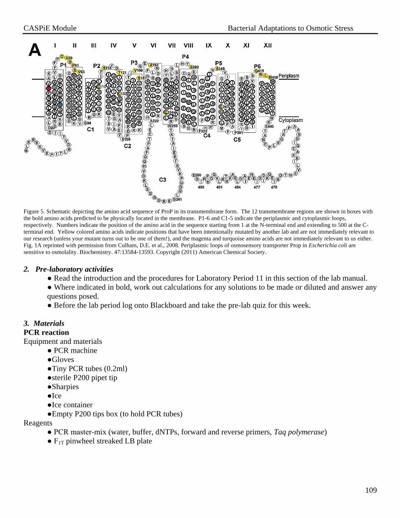
CASPiE Module Bacterial Adaptations to Osmotic Stress
109
Figure 5. Schematic depicting the amino acid sequence of ProP in its transmembrane form. The 12 transmembrane regions are shown in boxes with
the bold amino acids predicted to be physically located in the membrane. P1-6 and C1-5 indicate the periplasmic and cytoplasmic loops,
respectively. Numbers indicate the position of the amino acid in the sequence starting from 1 at the N-terminal end and extending to 500 at the C-
terminal end. Yellow colored amino acids indicate positions that have been intentionally mutated by another lab and are not immediately relevant to
our research (unless your mutant turns out to be one of them!), and the magenta and turquoise amino acids are not immediately relevant to us either.
Fig. 1A reprinted with permission from Culham, D.E. et al., 2008. Periplasmic loops of osmosensory transporter Prop in Escherichia coli are
sensitive to osmolality. Biochemistry. 47:13584-13593. Copyright (2011) American Chemical Society.
2. Pre-laboratory activities
● Read the introduction and the procedures for Laboratory Period 11 in this section of the lab manual.
● Where indicated in bold, work out calculations for any solutions to be made or diluted and answer any
questions posed.
● Before the lab period log onto Blackboard and take the pre-lab quiz for this week.
3. Materials
PCR reaction
Equipment and materials
● PCR machine
●Gloves
●Tiny PCR tubes (0.2ml)
●sterile P200 pipet tip
●Sharpies
●Ice
●Ice container
●Empty P200 tips box (to hold PCR tubes)
Reagents
● PCR master-mix (water, buffer, dNTPs, forward and reverse primers, Taq polymerase)
● F1T pinwheel streaked LB plate
CASPiE Module Bacterial Adaptations to Osmotic Stress
110
Agarose gel preparation
Equipment and materials
● Small gel apparatus (box, combs, voltage sources)
●Gloves
●Small flasks (120 ml for one gel)
●Microwave
●Balance
●Weigh paper/boats
●Weigh scoops
●Volumetric pipets or 50 mL graduated cylinders
●Lab tape
●P20 micropipeters
●P20 tips
●Small microcentrifuge tubes (1.5 mL)
●UV gel imager
●UV eyes shields/glasses
●Small microcentrifuge racks
Reagents
● MW ladder
●F1T plates
●Agarose
●Ethidium bromide
●TAE buffer (Tris base, Glacial acetic acid, EDTA)
●Loading buffer (bromophenol blue and glycerol)
Using BLAST and DNA alignments and sequencing
Equipment and materials
●Laptop computer
4. Procedures Part 1: PCR amplification
10. Make a note of the identity of your F1T that will be used today in your lab notebook.
11. Each group should obtain two PCR reaction tubes that contains the PCR master mix (Taq polymerase,
primers, and deoxynucleotides).
12. Label the PCR reaction tube with your initials on the top and the side of the tube with a sharpie.
13. Using a sterile p20 or p200 micropipette tip, tap a single colony from the appropriate F1. You do not
need to pick up the entire colony! Simply touching it with a sterile tip will provide you with enough
cells from which to amplify DNA.
14. Transfer the colony to the PCR reaction tube by placing the micropipette tip in the solution and swirl it a
few times. It may be necessary to gently blow on the tip to dislodge the colony, but please ask us
first!!!!
15. Carefully close your PCR reaction tube and bring it to us.
16. We will be also running the PCR with a tube that has no DNA. What is the purpose of this tube?
17. Once we have everyone’s samples, we will start the PCR thermal cycling for 30 cycles of denaturing,
annealing, and extension. This will take ~140 minutes. If we started with 109 cells in our colony,
how many copies of proP would we get after 30 cycles?
18. While the PCR is running, we will make our agarose gels.
CASPiE Module Bacterial Adaptations to Osmotic Stress
111
Part 2: Gel electrophoresis
1. Obtain a 125 ml flask.
2. Weigh out the appropriate amount of agarose using a balance. We want a 1% agarose gel in 50 ml
TAE Buffer. How much agarose do we need to weigh out?
3. Pour 50 ml of TAE buffer into the flask and gently swirl to mix the TAE buffer and agarose.
4. Microwave the flask 2-4 times for 1 minute each time. Between microwaving, take the flask out and
gently swirl. Keep microwaving for 1 minute each time until you do not see any white particles
floating around.
5. Let the flask cool down until it feels like a warm cup of coffee when you touch it. In the meantime,
place two pieces of tape over the exposed edges of your gel tray so that liquid will not leak out when
you pour it in.
6. Once the agarose and buffer has cooled, put on a pair of gloves and add 2.5 µL EtBr to the flask
and gently swirl. Please wear gloves from now on when handling the gel.
7. Slowly pour the gel into the tray and place the comb in the gel towards one of the edges. The gel
should solidify fully in 20-30 minutes.
8. Once the PCR reaction is finished, retrieve your sample(s) from the machine.
9. Obtain a tube of loading buffer and a small microcentrifuge tube
10. Label the microcentrifuge tube with the name of the mutant
11. Add 8 µL of your PCR reaction to the microcentrifuge tube.
12. Carefully add 1 µL of loading buffer to the tube. Close the tube and gently flick the tube to mix.
13. Carefully add 1 µL loading buffer to the tube of master mix given to you for your gel, close the tube,
and gently flick it to mix.
14. Three-four people will be sharing a single gel. Slowly remove the combs from the solidified gel.
15. Pour enough of the TAE buffer over the gel so that there is a 1cm or so thick layer of TAE buffer
over the gel. The buffer should completely cover the gel.
16. In the first lane, 9 µL of the ladder should be loaded. What is the purpose of the ladder?
17. In the second lane, 9 µL of the master mix should be loaded. Why would you want to run the
master mix out on the gel?
18. Your samples should be then loaded into the remaining wells.
19. We will help you hook the gel box up to the power supply and turn it on.
20. We will run the gel for ~ 45-60 minutes. You can watch the bromophenol blue move across the gel
and see the progress!
21. Once the gel is finished running, we will help you unhook the gel box from the power supply and we
will take it to a gel imager to illuminate it with UV light to see the DNA bands and assess our PCR
reaction.
22. If we obtain a single band at the proper location in the gel for proP, then our PCR was a success!
We can prepare your sample to send it over for sequencing!!
Part 2: Using BLAST and DNA alignments and sequencing
Follow the guidelines written in the handout Dr. Csonka created to sequence the proP gene
5. Post-laboratory analysis and results
● We will prepare your samples for sequencing and send them over. You will compare your mutant
sequence to wild type in lab next week.
6. Preparation for the Next Laboratory Activity
● You should read the introduction and procedures before going to your next laboratory period.
● Perform any calculations and answer any questions in your lab notebook as indicated in the manual
for Laboratory 12.

CASPiE Module Bacterial Adaptations to Osmotic Stress
112
● Take the online pre-lab quiz
XIII. Laboratory Period 12 – Sequencing and implications of point mutations in proP
Objectives
At the end of this laboratory period the students will be able to:
1. Describe the method for DNA sequencing
2. Appreciate the implications amino acid identity on protein structure and function
3. Understand membrane topology models for membrane proteins
6. Begin to understand the structure of ProP
7. Sequence a mutant gene and compare it to wild type
8. Translate DNA sequence into amino acid sequence
9. Formulate hypotheses regarding the phenotype of their mutants and their underlying genotype
1. Introduction
A. DNA sequencing methods
After amplification of our gene of interest, proP, we need to examine the nucleotide sequence to compare it to
the wild type sequence and see how it has changed. This involves a process, cleverly known as, sequencing the
gene, (protein coding region as well as the promoter), to determine the identity and order of the nucleotides.
Modern sequencing techniques very much resemble the process of PCR. Both processes involve taking DNA
and mixing it with primers, deoxynucleotides, and DNA polymerase and allowing transcription to proceed. The
important addition to the mix is small quantities of deoxynucleotides, known as dideoxynucleotides, that will
stop transcription.
Recall the structure of a nucleotide (Figure 1). Nucleotides are comprised of a ribose sugar, one or more
phosphate groups, and a nitrogenous base.
Figure 1. The chemical structure of the two classes of nucleotide bases in DNA and/or RNA. Public domain image from:
http://commons.wikimedia.org/wiki/File:Nucleotides.png
The sugar portion of the nucleotide has a free hydroxyl (-OH) group that can form a bond with the phosphate
group of an adjacent nucleotide (Figure 2). Dideoxynucleotides lack this free hydroxyl group, therefore if they
are added to the growing strand of DNA, transcription will halt because it cannot form a bond with another
nucleotide.

CASPiE Module Bacterial Adaptations to Osmotic Stress
113
Figure 2. The structure of deoxy- (dATP) and dideoxynucleotides (ddATP) and the bonds formed between nucleotides in the double-stranded DNA
helix. Dideoxynucleotides lack the free hydroxyl on their 3’ end that is necessary to form a bond with an adjacent nucleotide. This will halt
transcription/replication. Images from: http://commons.wikimedia.org/wiki/File:DATP_chemical_structure.png,
http://commons.wikimedia.org/wiki/File:DDATP_chemical_structure.png, and http://commons.wikimedia.org/wiki/File:DNA-labels.png.
This halting of transcription by the incorporation of the dideoxynucleotides can be exploited for determining the
nucleotide sequence of a gene. The dideoxynucleotides (ddATP, ddGTP, ddCTP, ddTTP) are added to the
sequencing mix at a low concentration relative to the levels of the deoxynucleuotides. In this way, the
probability of their incorporation into the growing strand is low and transcription will be halted randomly. For
example, if ddATP is included in the sequencing reaction at low levels, it will be incorporated randomly
opposite thymine, halting transcription of those strands. In this way, pieces of DNA of varying length will be
generated, all of which end with A. If the reaction is allowed to go through enough cycles, each reaction tube
will have DNA fragments of different sizes encompassing the entire complement of A’s. This process is
extended to include all four nucleotides in their dideoxy form. The samples are run on a gel to separate them
based on size, with single base differences in size being resolvable. The presence of the dideoxynucleotide is
visualized by a different fluorescent dye that was attached to each of the dideoxynucleotides (Figure 3).
Deoxynucleotide Dideoxynucleotide

CASPiE Module Bacterial Adaptations to Osmotic Stress
114
Figure 3. Schematic outlining the basic steps in DNA sequencing and an example of the chromatogram generated from a DNA sequencing gel. A –
Double-stranded DNA is denatured resulting in single-stranded DNA shown in B where an oligonucleotide primer complementary to the strand of
the DNA being sequenced is added to a tube containing DNA polymerase, four different deoxynucleotides, and four different dideoxynucleotides
each with a unique fluorescent label. C – The sequencing reaction is completed with the dideoxynucleotides incorporated randomly throughout the
sequence, forming different sized DNA fragments of the sequence. Fluorescent labels from these nucleotides are read by a laser after running the
fragments on a gel, forming a chromatogram shown in D. The position of a band on the gel provides information about the size of the DNA fragment
and the color of the signal provides the identity of the dideoxynucleotide. Image by Enzo at the Polish language Wikipedia [GFDL
(www.gnu.org/copyleft/fdl.html) or CC-BY-SA-3.0 (www.creativecommons.org/licenses/by-sa/3.0/)], from Wikimedia Commons. An animation depicting the steps in
DNA sequencing can be found at: http://www.dnalc.org/resources/animations/cycseq.html.
A computer can be used to quickly scan the gels and sort through the position of the various fluorescent signals
on the gel and provide an ordering of the nucleotides. As the computer scans the gel, the intensity of the
fluorescent signal is quantified as is its position in the gel to create a plot of the different fluorescent signals
known as a chromatogram (Figure 3D). Based on the fact that each fragment will migrate to a position on the
gel that is inversely proportional to the number of nucleotides it contains, the size of the fragment can be
determined. In addition, because each dideoxynucleotide is labeled with a different fluorescent dye, the identity

CASPiE Module Bacterial Adaptations to Osmotic Stress
115
of the nucleotide at the end of each fragment can be determined. The more discreet and large the signal is on
the spectrogram, the more confident one can be that the nucleotide is identified correctly (Figure 3D).
There are 1500 nucleotides in the proP gene, which is quite large. Therefore, we are sequencing with the use of
multiple primers (6) that are complementary to various regions flanking and within the gene. In this way we
will ensure that the entire gene is transcribed between the 6 primers. Each of the primers will be in separate
reactions which will provide us with 6 pieces of sequence that will overlap to some degree. This overlap is
useful in helping us determine if any deviations from our mutant sequence are a result of a mutation or simply a
sequencing error. With any luck, our mutations will be found in 2 or more sequencing fragments which will
strengthen the support that it is indeed a mutation!
B. Structure and properties of amino acids
Once we have identified the mutation in the nucleotide sequence of our proP mutants, we will translate that
sequence into the amino acid sequence to examine the consequences of that single nucleotide change at the
level of the protein. We will see where in the protein the change is made and, depending on the identity of the
new amino acid compared to the one encoded by the wild type gene, try to imagine what such a change might
be doing to alter the funcitoning of the ProP transporter.
Amino acids are similar to nucleotides in that they both have a base composition that is shared across their
members. In amino acids, this is an alpha carbon to which are attached an amino group, a carboxl group, a
hydrogen, and an R side group (variant) (Figure 4). The R group is what varies across the different types of
amino acids and gives them their unique properties.
Figure 4. The basic structure of an amino acid. Public domain image from: http://en.wikipedia.org/wiki/File:AminoAcidball.svg
Based on the properties of their R groups, amino acids are categorized accordingly: (1) nonpolar and
hydrophobic, (2) polar and uncharged, (3) negatively charged/acidic, and (4) positively charged/basic (Figure
5). When we are thinking about a protein that exists in a membrane, like ProP, for example, the properties of
the amino acids are going to influence which portions of the protein are likely to be found within the plasma
membrane versus in aqueous environments intra- and extracellularly. For example, the nonpolar amino acids
like valine and leucine are more likely to be found in regions of the protein that traverse the plasma membrane
or are folded away from the aqueous environments within the tertiary structure of the protein. Amino acids
such as arginine, in contrast, are more likely to be found in aqueous environments inside or outside of the cell.
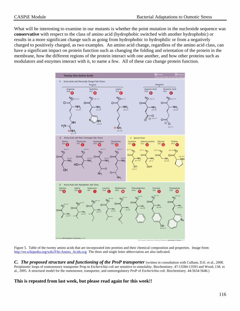
CASPiE Module Bacterial Adaptations to Osmotic Stress
116
What will be interesting to examine in our mutants is whether the point mutation in the nucleotide sequence was
conservative with respect to the class of amino acid (hydrophobic switched with another hydrophobic) or
results in a more significant change such as going from hydrophobic to hydrophilic or from a negatively
charged to positively charged, as two examples. An amino acid change, regardless of the amino acid class, can
have a significant impact on protein function such as changing the folding and orientation of the protein in the
membrane, how the different regions of the protein interact with one another, and how other proteins such as
modulators and enzymes interact with it, to name a few. All of these can change protein function.
Figure 5. Table of the twenty amino acids that are incorporated into proteins and their chemical composition and properties. Image from:
http://en.wikipedia.org/wiki/File:Amino_Acids.svg The three and single letter abbreviation are also indicated.
C. The proposed structure and functioning of the ProP transporter (written in consultation with Culham, D.E. et al., 2008.
Periplasmic loops of osmosensory transporter Prop in Escherichia coli are sensitive to osmolality. Biochemistry. 47:13584-13593 and Wood, J.M. et
al., 2005. A structural model for the osmosensor, transporter, and osmoregulatory ProP of Escherichia coli. Biochemistry. 44:5634-5646.)
This is repeated from last week, but please read again for this week!!
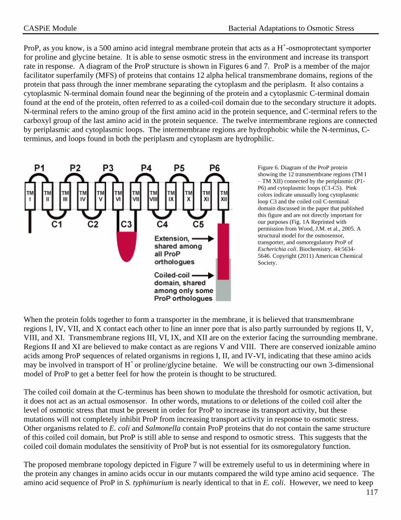
CASPiE Module Bacterial Adaptations to Osmotic Stress
117
ProP, as you know, is a 500 amino acid integral membrane protein that acts as a H+-osmoprotectant symporter
for proline and glycine betaine. It is able to sense osmotic stress in the environment and increase its transport
rate in response. A diagram of the ProP structure is shown in Figures 6 and 7. ProP is a member of the major
facilitator superfamily (MFS) of proteins that contains 12 alpha helical transmembrane domains, regions of the
protein that pass through the inner membrane separating the cytoplasm and the periplasm. It also contains a
cytoplasmic N-terminal domain found near the beginning of the protein and a cytoplasmic C-terminal domain
found at the end of the protein, often referred to as a coiled-coil domain due to the secondary structure it adopts.
N-terminal refers to the amino group of the first amino acid in the protein sequence, and C-terminal refers to the
carboxyl group of the last amino acid in the protein sequence. The twelve intermembrane regions are connected
by periplasmic and cytoplasmic loops. The intermembrane regions are hydrophobic while the N-terminus, C-
terminus, and loops found in both the periplasm and cytoplasm are hydrophilic.
When the protein folds together to form a transporter in the membrane, it is believed that transmembrane
regions I, IV, VII, and X contact each other to line an inner pore that is also partly surrounded by regions II, V,
VIII, and XI. Transmembrane regions III, VI, IX, and XII are on the exterior facing the surrounding membrane.
Regions II and XI are believed to make contact as are regions V and VIII. There are conserved ionizable amino
acids among ProP sequences of related organisms in regions I, II, and IV-VI, indicating that these amino acids
may be involved in transport of H+
or proline/glycine betaine. We will be constructing our own 3-dimensional
model of ProP to get a better feel for how the protein is thought to be structured.
The coiled coil domain at the C-terminus has been shown to modulate the threshold for osmotic activation, but
it does not act as an actual osmosensor. In other words, mutations to or deletions of the coiled coil alter the
level of osmotic stress that must be present in order for ProP to increase its transport activity, but these
mutations will not completely inhibit ProP from increasing transport activity in response to osmotic stress.
Other organisms related to E. coli and Salmonella contain ProP proteins that do not contain the same structure
of this coiled coil domain, but ProP is still able to sense and respond to osmotic stress. This suggests that the
coiled coil domain modulates the sensitivity of ProP but is not essential for its osmoregulatory function.
The proposed membrane topology depicted in Figure 7 will be extremely useful to us in determining where in
the protein any changes in amino acids occur in our mutants compared the wild type amino acid sequence. The
amino acid sequence of ProP in S. typhimurium is nearly identical to that in E. coli. However, we need to keep
Figure 6. Diagram of the ProP protein
showing the 12 transmembrane regions (TM I
– TM XII) connected by the periplasmic (P1-
P6) and cytoplasmic loops (C1-C5). Pink
colors indicate unusually long cytoplasmic
loop C3 and the coiled coil C-terminal
domain discussed in the paper that published
this figure and are not directly important for
our purposes (Fig. 1A Reprinted with
permission from Wood, J.M. et al., 2005. A
structural model for the osmosensor,
transporter, and osmoregulatory ProP of
Escherichia coli. Biochemistry. 44:5634-
5646. Copyright (2011) American Chemical
Society.
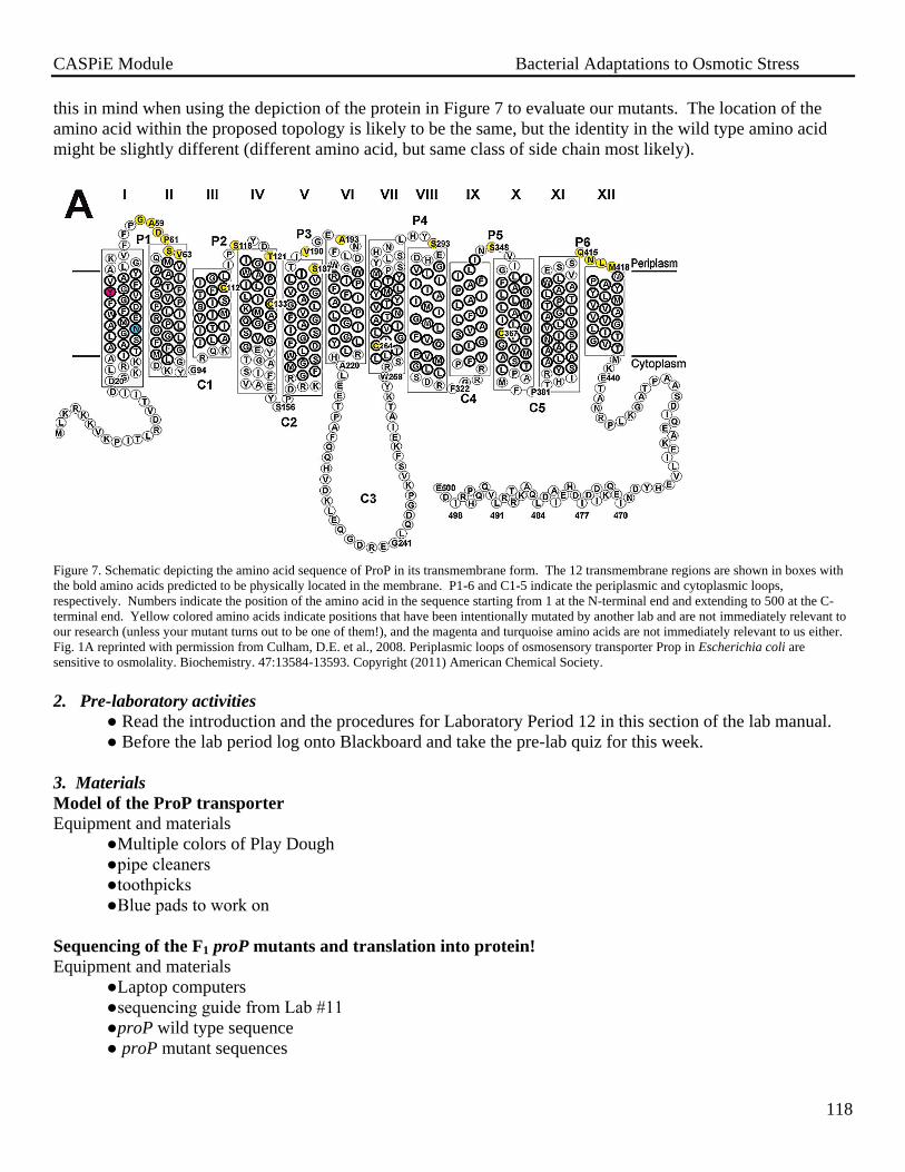
CASPiE Module Bacterial Adaptations to Osmotic Stress
118
this in mind when using the depiction of the protein in Figure 7 to evaluate our mutants. The location of the
amino acid within the proposed topology is likely to be the same, but the identity in the wild type amino acid
might be slightly different (different amino acid, but same class of side chain most likely).
Figure 7. Schematic depicting the amino acid sequence of ProP in its transmembrane form. The 12 transmembrane regions are shown in boxes with
the bold amino acids predicted to be physically located in the membrane. P1-6 and C1-5 indicate the periplasmic and cytoplasmic loops,
respectively. Numbers indicate the position of the amino acid in the sequence starting from 1 at the N-terminal end and extending to 500 at the C-
terminal end. Yellow colored amino acids indicate positions that have been intentionally mutated by another lab and are not immediately relevant to
our research (unless your mutant turns out to be one of them!), and the magenta and turquoise amino acids are not immediately relevant to us either.
Fig. 1A reprinted with permission from Culham, D.E. et al., 2008. Periplasmic loops of osmosensory transporter Prop in Escherichia coli are
sensitive to osmolality. Biochemistry. 47:13584-13593. Copyright (2011) American Chemical Society.
2. Pre-laboratory activities
● Read the introduction and the procedures for Laboratory Period 12 in this section of the lab manual.
● Before the lab period log onto Blackboard and take the pre-lab quiz for this week.
3. Materials
Model of the ProP transporter
Equipment and materials
●Multiple colors of Play Dough
●pipe cleaners
●toothpicks
●Blue pads to work on
Sequencing of the F1 proP mutants and translation into protein!
Equipment and materials
●Laptop computers
●sequencing guide from Lab #11
●proP wild type sequence
● proP mutant sequences

CASPiE Module Bacterial Adaptations to Osmotic Stress
119
4. Procedures Part 1: Constructing a 3-D model of the ProP protein
1. Using the structural information summary provided in this manual, each pair should obtain 3
different colors of Play dough and some pipe cleaners.
2. Create cylinders to represent transmembrane domains. Use different colors to represent the different
groupings of the transmembrane domains.
3. You can use a toothpick to etch in the transmembrane domain numbers on the cylinders.
4. Use the pipe cleaners to link the transmembrane domains with their periplasmic and intracellular
loops and termini.
Part 2: Sequencing of the F1 proP mutants!!!
1. Download the sequence for your mutants from the folder with your initials in the Lab 12 folder.
2. Using the guide provided last week by Dr. Csonka, compare your F1 mutant proP sequence to the wild
type sequence.
3. Take that sequence and wild type and translate it into protein.
4. Compare the two sequences to identify any amino acid change that resulted from your mutation in the
gene!!
5. Think about the significance of any changes based on where it is in the protein and what the change was
(conservative vs. nonconservative amino acid changes).
6. Place a dob of red Play Dough on your model to indicate the approximate location of the mutations and
mark it on the overhead of the protein.
7. Formulate hypotheses to link together the results of your GB antagonism and proline uptake plates, the
doubling times (if you have them for your sequenced mutant) and the location and identity of the amino
acid change in the ProP protein. Imagine a mechanism!!!
Part 3: Poster!
You will begin by sketching out a plan for your poster with the organization and content (data, graphs, photos
of plates, schematics, etc) that we will give you feedback on (poster mock-up). You should start work on your
poster this week!! There are two example posters from last year that you can use as a template. They are two
Powerpoint files with the proper dimensions for printing and good font sizes. Feel free to alter color schemes.
If you would like access to different schematics from the lab manuals to use in your poster, let us know and we
can get you those.
5. Post-laboratory analysis and results
●Think about the implications of your mutations.
●Read papers, talk about it, ask questions!!!
6. Preparation for the Next Laboratory Activity
● Continue thinking about the implications of your mutations
● Add the PCR and sequencing methods to that portion of your poster.
● Work on your poster with your group
CASPiE Module Bacterial Adaptations to Osmotic Stress
120
Appendix A - Bacterial Genetics Strain List
Strain Genotype Phenotype
TL-1 Wild type Wild type (not an auxotroph)
TL-117 proAB- Proline auxotroph
TL-602 his- Histidine auxotroph
TL-4127 pyrB- Uracil auxotroph
TL-197 proP-, proU
+, betP
+ No ProP transport
TL-201 proP-, proU
-, betP
+ No ProP or ProU transport
TL-4088 proP-, proU
-, betP
- No proline or GB transport
TL-193 proAB-, proP
+, proU
-, putP
- Proline auxotroph, no PutP or ProU transport
TL-1673 proAB-, proP
+, proU
-, putP
-,
melA-
Proline auxotroph, no ProU or PutP transport.
Unable to grow on melibiose as a sole carbon source
TL-4500 proAB-, proP
+, proU
-, putP
-,
melA-, mutT
-
Proline auxotroph, no ProU or PutP transport.
Unable to grow on melibiose as a sole carbon
source. Unable to use MutT to correct DNA
mistakes
TL-1901 proP- No ProP transport. Chloramphenicol resistant
TL-4513 proAB-, proU
-, putP
-, proP
- Proline auxotroph, no proline transport through
standard proline transport systems

CASPiE Module Bacterial Adaptations to Osmotic Stress
121
Appendix B - Bacterial Genetics Implementation Material
Week 1
Reagent Preparation - Osmosis Exercise
o Isotonic sucrose solution (5% sucrose in water)
o Hypertonic sucrose solution (20% sucrose in water)
- Aseptic Technique Exercise
o Sterile liquid LB media
Tryptone – 10 g/L
Yeast Extract – 5 g/L
Sodium Chloride – 5 g/L
Deionized Water – 1 L
o 5 mL LB in test tubes, 4 test tubes/person = 20 mL LB/person
Week 2
Reagent Preparation - Dilutions Exercise
o Blue water stock solution
10 drops blue food coloring in 200 mL H2O
- Media Preparation Exercise
o Solid minimal media (M63)
10X M63 Salt Solution
Potassium Hydroxide (KOH) – 0.75 M (42.0 g/L)
Monobasic Potassium Phosphate (KH2PO4) – 1.0 M (136.0 g/L)
Ammonium Sulfate (NH4)2SO4 – 0.15 M (20.0 g/L)
1000X Magnesium Sulfate-Iron Sulfate solution (MgSO4-FeSO4)
Magnesium Sulfate – 0.16 M (4.0 g/100mL MgSO4 ● 7H2O or 1.95 g/100mL MgSO4)
Iron Sulfate – 1.8 mM (0.050 g/100mL FeSO4 ● 7H2O)
40 mL salt solution per person
o Sterile glucose solution (2M in water)
o 1 M NaOH solution (does not need to be sterile)
- Quadrant Streaking Exercise
o LB plates
Tryptone – 10 g/L
Yeast Extract – 5 g/L
Sodium Chloride – 5 g/L
Agar – 20 g/L
Deionized Water – 1 L
1 L of LB makes approximately 30 plates
o At least 1 LB plate/person
- Spread Plating Exercise
o LB plates
o 2 LB plates/person or group

CASPiE Module Bacterial Adaptations to Osmotic Stress
122
Organism Preparation - Quadrant Streaking Exercise
o One mixed culture of bacteria per group (Escherichia coli, Serratia marcescens, and Bacillus cereus) in
LB broth
Bacteria should be grown over night (O/N) in separate LB cultures at 30ºC and should be mixed
in equal proportions into sterile tubes
1 mL of mixed culture is plenty for each group of students
- Spread Plating Exercise
o Undiluted culture of Salmonella typhimurium LT2 TL-1 grown O/N in liquid LB broth at 30 or 37ºC.
o Diluted culture of Salmonella typhimurium LT2 TL-1
Dilute 106 fold in sterile saline (0.9% NaCl in H2O) or liquid M63 media without glucose
Week 3
Reagent Preparation - Continuation of Quadrant Streaking Exercise
o 2 LB plates per pair of students
- Auxotrophy Exercise
o M63 glucose plates
Sterile M63 glucose media plus 20 g/L agar
Autoclave agar and 600 mL of water in one flask and 10x stock solution plus 300 mL of water in
another flask
Add agar mix to the stock solution mix flask after autoclaving.
Add sterile 2M glucose for a final concentration of 10 mM after autoclaving
5 plates per person or group – 1L of media makes about 30 plates
o Sterile proline stock solution (100 mM in water) – 1 mL per group
Sterilize by autoclaving 15-20 minutes
o Sterile histidine stock solution (100 mM in water) – 1 mL per group
Sterilize by autoclaving 15-20 minutes
o Sterile uracil stock solution (20 mM uracil in water) – 1 mL per group
Sterilize by autoclaving 15-20 minutes
o Mixed solution of sterile proline, histidine, and uracil (Mix separate solutions in equal proportions) – 1
mL per group
- High Osmolarity Stimulation Exercise
o M63 glucose plates (1 per group)
o M63 glucose + 0.65 M NaCl plates (3 per group)
Sterile M63 glucose media preparation
Add 0.65 M NaCl to stock solution and mix before autoclaving
1 L of media makes about 30 plates
o Sterile proline stock solution (10 mM in water)
Sterilize by autoclaving 15-20 minutes
o Sterile glycine betaine stock solution (100 mM in water)
pH adjust solution to 7.2
Sterilize by autoclaving 15-20 minutes
- Glycine Betaine Antagonism Experiment
o M63 glucose + 0.3 M NaCl plates (1 per group)
o M63 glucose + 0.3 M NaCl + 0.1 mM proline plates (4 per group)
o M63 glucose + 0.3 M NaCl + 0.1 mM proline + 2 mM glycine betaine plates (1 per group)
o Sterile glycine betaine stock solution (50 mM in water)
pH adjust solution to 7.2
Sterilize by autoclaving 15-20 minutes
- Microscope and Osmotic Stress Exercise

CASPiE Module Bacterial Adaptations to Osmotic Stress
123
o Red blood cells
o Hypertonic solution from week 1
Organism Preparation
- Auxotrophy Exercise
o TL-1 culture plate (1 per every 2 groups)
o TL-117 culture plate (1 per every 2 groups)
o TL-602 culture plate (1 per every 2 groups)
o TL-4127 culture plate (1 per every 2 groups)
o All plates grown O/N at 37ºC
- High Osmolarity Stimulation Exercise
o TL-1 culture plate (1 per every 2 groups)
o TL-197 culture plate (1 per every 2 groups)
o TL-201 culture plate (1 per every 2 groups)
o TL-4088 culture plate (1 per every 2 groups)
o All plates grown O/N at 37ºC
- Glycine Betaine Antagonism Exercise
o TL-1 culture plate (1 per every 2 groups)
o TL-117 culture plate (1 per every 2 groups)
o TL-193 culture plate (1 per every 2 groups)
o All plates grown O/N at 37ºC
Week 4
Reagent Preparation - Maximum Absorbance Exercise
o Blue water stock solution from week 2 (Stock A)
o 1:1 dilution of Stock A (Stock B)
- Bacterial Growth Rate Exercise
o Sterile M63 glucose + 0.1 mM proline broth
Sterile M63 media supplemented w/ 20 mM glucose and 0.1 mM proline
o 20 mL broth in separate sterile Erlenmeyer flasks with foam plugs or aluminum foil (1 per student)
Organism Preparation - Bacterial Growth Rate Exercise
o O/N cultures of TL-4553 and previously generated ProP mutants in M63 media
Two days before lab, start O/N cultures of TL-4553 (wildtype) and previously generated mutants
(TL-4554, TL-4555, TL-4556, TL-4557, TL-4558, and TL-4559) in 2 mL LB media. Grow at
37ºC.
After O/N growth, inoculate 50 μl of each culture into 5 mL M63 glucose media + 1 mM proline
and grow O/N at 37ºC.
Inoculate O/D growth curve cultures at a starting OD600 of around 0.08.
Week 5
Reagent Preparation - Standard Curve Construction and Interpolation of Unknown Exercise
o Stock A and Stock B from Week 4
o “Unknown” dilution of Stock B
- Mutagenesis and Mutation Frequency Exercise
o M63 glucose + 0.1 mM proline plates (2 per person)
Add proline before autoclaving

CASPiE Module Bacterial Adaptations to Osmotic Stress
124
o M63 glucose + 0.1 mM proline + 2 mM glycine betaine plates (1 per person)
Add proline and glycine betaine before autoclaving
o EMS for chemical mutagenesis
o Sterile saline (0.9%) or M63 media with no glucose as a diluent
Organism Preparation - Mutagenesis and Mutation Frequency Exercise
o O/N LB culture of TL-1673 (grown at 37ºC) for spontaneous mutagenesis
o O/N LB culture of TL-4500 (grown at 37ºC) for mutator strain mutagenesis
Week 6
Reagent Preparation - Pinwheel Streaking of Mutants Exercise
o M63 glucose + 0.1 mM proline + 2 mM glycine betaine plates (1 per person)
- Inoculation of Liquid Media Exercise
o Tube of sterile LB media (1 per student)
Organism Preparation - Inoculation of Liquid Media
o Plate culture of TL-1 (or any other bacterial species capable of growth in LB media)
Week 7
Reagent Preparation - Transduction Exercise
o LB plates supplemented with 12.5 μg/mL chloramphenicol (13 per student)
- Gram Staining Exercise
o Gram stain reagents (Crystal violet, iodine, Gram’s alcohol, and safranin)
Organism Preparation - Transduction Exercise
o O/N cultures of F1 mutants inoculated into individual LB tubes two days before lab and grown at 37ºC
o P22 lysate grown on TL-1901 inoculated into the F1 mutant cultures at a 1:10 ratio of lysate:culture and
grown O/N at 37ºC one day before lab
o O/N culture of TL-4513 inoculated into LB media and grown at 37ºC the day before lab (2 ml per person)
- Gram Staining Exercise
o O/N culture of bacteria in LB broth grown at 37ºC
o Gram negative rod (Salmonella species), Gram positive rod (Bacillus species), and Gram positive cocci
(Staphylococcus species). Other organisms can be substituted.
Week 8
Reagent Preparation - Pinwheel Streak Transductant Exercise
o LB plates supplemented with 12.5 μg/mL chloramphenicol (5 per student)
Organism Preparation - Pinwheel Streak Transductant Exercise
o Students will need their transduction plates (grown at 37ºC 12-24 hours or until suitable size colonies
appear) from week 7
o Students should pinwheel streak 5 transductants from each plate onto the LB chloramphenicol plates

CASPiE Module Bacterial Adaptations to Osmotic Stress
125
Week 9
Reagent Preparation - Transductant Screening Exercise
o M63 glucose plates (1 per student
o M63 glucose + 0.1 mM proline plates (1 per student)
o M63 glucose + 0.1 mM proline + 2 mM glycine betaine plates (1 per student)
o LB plates supplemented with 20 μg/mL tetracycline (1 per student)
o LB plates supplemented with 12.5 μg/mL chloramphenicol (1 per student)
Organism Preparation - Transductant Screening Exercise
o Students will need the pinwheel streak transductants plates from week 8
Week 10
Reagent Preparation - Glycine Betaine and Proline Uptake Plate Assay Exercise
o Sterile 2 M glycine betaine solution
pH adjust to 7.2
Sterilize by autoclaving
o Sterile 100 mM proline solution
Sterilize by autoclaving
o M63 glucose plates (8 per group)
o M63 glucose + 0.1 mM proline plates (8 per group)
o M63 glucose + 0.3 M NaCl + 0.1 mM proline plates (8 per group)
o M63 glucose + 0.3 M NaCl plates (8 per group)
- Second Bacterial Growth Rate Exercise
o Sterile M63 glucose + 0.1 mM proline broth
20 mL in flasks just as in week 4
One flask for every potential proP mutant
Sterile saline (0.9%) or M63 broth with no glucose as a diluent
Organism Preparation - Glycine Betaine and Proline Uptake Plate Assay Exercise
o Students will need the pinwheel streak plate of their original mutants and the transductants
- Second Bacterial Growth Rate Exercise
o Two days before lab, start O/N cultures of potential proP mutants in 2 mL LB media. Grow at 37ºC.
o After O/N growth, inoculate 50 μl of each culture into 5 mL M63 glucose media + 1 mM proline and
grow O/N at 37ºC.
o Inoculate O/D growth curve cultures at a starting OD600 of around 0.08.
Week 11
Reagent Preparation - PCR Amplification and Agarose Gel Exercise
o PCR master-mix (1 per potential proP mutant)
Water
Buffer
dNTPs

CASPiE Module Bacterial Adaptations to Osmotic Stress
126
forward and reverse primers complementary to proP
Taq polymerase
o Molecular weight ladder
o 1X TAE buffer
50 mL per gel
Each gel can support two groups
o Loading buffer
o Ethidium bromide
o Ethanol precipitation of successful PCR fragments
o Sequencing facility capable of low throughput DNA sequencing and all relevant sequencing reagents
Six complementary proP primers
Organism Preparation - PCR Amplification Exercise
o Students will need a plate culture of their potential proP mutant
Week 12
Reagent Preparation - Model Construction of the ProP Transporter
o Multiple colors of Play Dough
o Pipe cleaners
o Toothpicks

CASPiE Module Bacterial Adaptations to Osmotic Stress
127
References and image information
References
Alberts B, Johnson A, Lewis J, Raff M, Roberts K, and Walter P. Molecular Biology of the Cell, Garland
Science; 5 edition (November 16, 2007)
Becker WM, Kleinsmith LJ, and Hardin J (2003). Guide to Microscopy. Benjamin/Cummings Pub. Co
Caetano-Anollés G, Yafremava LS, Gee H, Caetano-Anollés D, Kim HS, Mittenthal JE (2008) The origin and
evolution of modern metabolism. Int J Biochem Cell Biol. Feb;41(2):285-97.
Cánovas D, Fletcher SA, Hayashi M, Csonka LN (2001) Role of trehalose in growth at high temperature of
Salmonella enterica serovar Typhimurium. J Bacteriol. Jun;183(11):3365-71.
Chrispeels MJ and Agre P (1994) Aquaporins: water channel proteins of plant and animal cells. Trends
Biochem Sci. Oct;19(10):421-5.
Culham DE, Vernikovska Y, Tschowri N, Keates RA, Wood JM, Boggs JM (2008) Periplasmic loops of
osmosensory transporter ProP in Escherichia coli are sensitive to osmolality. Biochemistry 47, 13584-13593.
Davidson AL, Dassa E, Orelle C, Chen J (2008) Structure, function, and evolution of bacterial ATP-binding
cassette systems. Microbiol Mol Biol Rev. Jun;72(2):317-64
Dunlap, V. J., and Csonka, L. N. (1985). Osmotic regulation of L-proline transport in Salmonella typhimurium.
J. Bacteriol. 163, 296-304.
Karp G. Cell and Molecular Biology: Concepts and Experiments, John Wiley & Sons Inc , 4th
Edition
Kruse E, Uehlein N, Kaldenhoff R (2006) The aquaporins. Genome Biol. 7(2):206.
Kühlbrandt W (2004) Biology, structure and mechanism of P-type ATPases. Nat Rev Mol Cell Biol.
Apr;5(4):282-95.
Loukin SH, Kuo MM, Zhou XL, Haynes WJ, Kung C, Saimi Y (2005) Microbial K+ channels. J Gen Physiol.
125(6):521-7.
McClelland M, Sanderson KE, Spieth J, Clifton SW, Latreille P, Courtney L, Porwollik S, Ali J, Dante M, Du
F, Hou S, Layman D, Leonard S, Nguyen C, Scott K, Holmes A, Grewal N, Mulvaney E, Ryan E, Sun H,
Florea L, Miller W, Stoneking T, Nhan M, Waterston R, Wilson RK (2001) Complete genome sequence of :
Salmonella enterica: serovar Typhimurium LT2. Nature, Oct 25;413(6858):852-6
Russell et al., 2008.
http://www.ncbi.nlm.nih.gov.login.ezproxy.lib.purdue.edu/pubmed?term=%22Fletcher%20SA%22%5BAuthor%5D

CASPiE Module Bacterial Adaptations to Osmotic Stress
128
Salisbury FB and Ross CW Plant Physiology . International Thomson Publishing; 4r.e. edition (1991)
Snyder L and Champness W . Molecular Genetics of Bacteria ASM Press; 3 edition (May 31, 2007)
Willey J, Sherwood S, Woolverton C. Prescott, Harley, and Klein’s Microbiology, McGraw-Hill
Science/Engineering/Math; 7 edition (January 12, 2007).
Wood, JM, Culham DE, Hillar A, Vernikovska YI, Liu F, Boggs JM, Keates RA (2005) A structural model for
the osmosensor, transporter, and osmoregulatory ProP of Escherichia coli. Biochemistry. 44:5634-5646
Wood JM (2007) Bacterial osmosensing transporters. Methods Enzymol 428:77-107.
Image information
All images without a specific attribution were generated by the authors of this manual (BJ Gasper and SM
Gardner). Public domain images are noted as such and/or simply attributed with the appropriate weblink.
Other images are filed under the Creative Commons Attribution-Share Alike 3.0 Unported license and
permission was granted under the GNU Free Documentation License, Version 1.2. A copy of this license and
its terms can be found at:
http://commons.wikimedia.org/wiki/Commons:GNU_Free_Documentation_License_1.2
ASM Microbe Library images
Laboratory period 2, Figure 6.
Liao MK, MacWilliams MP. Luria Broth (LB) and Luria Agar (LA) Media and Their Uses: Escherichia coli.
Visual Resources. American Society for Microbiology, Washington, DC. www.microbelibrary.org Accessed
30 December 2011.
Laboratory period 3, Figure 15
Sturm T. Staphylococcus aureus, a gram-positive coccus. Visual Resources. American Society for
Microbiology, Washington, DC. www.microbelibrary.org Accessed 30 December 2011.
Sturm T. Escherichia coli, a gram-negative bacillus. Visual Resources. American Society for Microbiology,
Washington, DC. www.microbelibrary.org Accessed 30 December 2011.


![Supporting Online Material forscience.sciencemag.org/highwire/filestream/590781/field_highwire...Verde [Guanacaste] Biological Stations, 2006; Corcovado National Park [Puntarenas],](https://static.fdocuments.us/doc/165x107/5e215cb3bf01800aa4125a36/supporting-online-material-guanacaste-biological-stations-2006-corcovado-national.jpg)