Supporting Information

1 Fitting the K-pairwise maximum entropy model todata

To identify the values λ of the model parameters which yield the best fit of the maximumentropy model to data, we maximise the log-likelihood of the model given the data. Thegeneral form of the log-likelihood of a maximum entropy model parametrised by vectorλ is given by

L(λ) =

M∑m=1

logP (x(m)|λ) = −M logZλ +

M∑m=1

λ>f(x(m)) (1)

for the spike-data vectors x(m) ∈ {0, 1}n, m = 1, . . . ,M and (usually intractable)normalizer Zλ,

Zλ =∑x

exp(λ>f(x)

).

Every choice of the feature function f defines a specific maximum entropy model overthis n-dimensional binary space. For the K-pairwise maximum entropy model used inthis paper, f(x) ∈ {0, 1}n(n+3)/2+1 is composed of:

1. n first-order features

fi(x) = xi,

with corresponding parameters collected in h. The hi, i = 1, . . . , n control single-cellfiring rates (in units of bins rather than Hz).

2. n(n− 1)/2 second-order features

fij(x) = xixj ,

with parameters Jij , j, i = 1, . . . , n, i < j, controlling pairwise neuronal correla-tions.

3. n+1 population-scale features

fk(x) =

{1, if

∑i xi = k

0, otherwise

with parameters Vk, k = 0, . . . , n. The vector V controls the overall number ofspikes in each temporal bin.

Note that that there is some degeneracy between the parameter vectors V and bothh and J —a global upwards shift of firing rates for example can be achieved both byadding a positive constant ε to each hi, or by adding εk to each of the Vk. Similarly,

adding a constant ε to every Jij can be balanced by subtracting εk(k−1)2 from each Vk.

Since either manipulation of V is zero for k = 0, fixing Vk=0 = 0 is not sufficient forgetting rid of this parameter degeneracy. As we never interpreted the parameter-values

1/27

themselves, but only the fit to data, we made no attempt to add additional constraintsto achieve a unique parameterization.

We can re-write the K-pairwise model into the general maximum entropy form bystacking the feature functions fi, fij , and fk into the vector-valued feature functionf and doing the same with parameters hi, Jij , and Vk to obtain λ = {h, J, V } ∈Rn(n+3)/2+1. The derivative of the log-likelihood with respect to any single parameterλl, l = 1, . . . , n(n+ 3)/2 + 1 is given by (see e.g. [1])

δ

δλl

M∑m=1

logP (x(m)|λ) =δ

δλl

M∑m=1

(λ>f(x(m))− logZλ

)=

M∑m=1

δ

δλlλ>f(x(m))− δ

δλlM log

∑x

exp(λ>f(x)

)=

M∑m=1

fl(x(m))−M

∑x λl exp

(λ>f(x)

)∑x exp (λ>F (x))

= M

(1

M

M∑m=1

fl(x(m))− Eλ[fl(x)]

). (2)

As can be seen from equation (2), the gradient of the log-likelihood vanishes if and onlyif the data means match the expectations of f(x) under the model.

To deal with data-sets of limited size, we maximised a regularised variant of the log-likelihood,

L(h, J, V |σh, σJ ,Σ) : =

M∑m=1

logP (x(m)|h, J, V )− 1

σh‖h‖1 −

1

σJ‖J‖1 −

1

2V >Σ−1V (3)

Σ = (σSS + σII)−1

σS + σIS0•S0•

>

Skk′ = exp

(− (k − k′)2

2τ2S

)S0k = σS exp

(− k2

2τ2S

).

Here, the matrix Σ implements a combined ridge and smoothing regression over V ,with (n + 1) × (n + 1) identity matrix I and smoothing matrix S corresponding to asquared-exponential kernel [2]. We set V0 = 0 and accounted for this by conditioning onV0 and correspondingly subtracted S0•(σS +σI)

−1S0•> from Σ. We used σh = σJ = 104,

σS = 10, σI = 400 and τS = 10.

To fit maximum entropy models to large neural populations, one needs to first approxi-mate the feature moments Eλ[f(x)] needed for the gradients of both eq. (1) and eq. (3)also for large populations (n > 20), and then update the parameters λ.

We introduce two modifications over previous approaches to fitting maximum entropymodels to neural data [3] to improve computational efficiency: First, we used pairwiseGibbs sampling and Rao-Blackwellisation to considerably improve estimation of thesecond-order feature moments Eλ[fij(x)], and Second, we follow the authors of [4], whodescribed a trick for efficiently updating the parameters in pairwise binary maximumentropy models: If one restricted updates to coordinate-wise updates, then one cancalculate the gain from updating a single variable in closed form, which makes it easy toselect both the variable to update as well as the step-length in closed form. We show howthis trick can be extended to allow a joint update of all the population-count features

2/27

V . In addition, the gain in log-likelihood is linear in the feature-moments, which makesit possible to compute it from a running average over the MCMC sample, and avoidshaving to store the entire sample in memory at any point. We describe our contributionsin the sections 1.1 and 1.2, respectively.

1.1 Pairwise Gibbs sampling and Rao-Blackwellisation

Following previous work [1], we used MCMC sampling to approximate the expectationsof the feature functions f(x) under the K-pairwise model with parameters λ. Theseexpected values Eλ[f(x)] are required to evaluate the gradients of the (penalised) log-likelihood, as well as the log-likelihood gains resulting from parameter updates. Asthe number of pairwise terms grows quadratically with population size n, most of theparameters of the model P (x|λ) for large n control pairwise moments Eλ[xixj ]. To makethe estimation of these pairwise interactions more efficient, we implemented a pairwiseGibbs sampler that for each update step of the Markov chain samples two variablesxi and xj , i 6= j, i, j ∈ 1, . . . , n. This furthermore allowed us to ’Rao-Blackwellise’ thesingle-cell and pair-wise feature components fi(x) = xi and fij(x) = xixj [5–8]. i.e. touse the conditional probabilities P (xi = 1|x∼i, λ) and P (xixj = 1|x∼{i,j}, λ) for momentestimation, instead of the binary xi and xixj .

The Rao-Blackwell theorem states that the variance of the Rao-Blackwellized estimatorsis equal or (as in our case) smaller than that of the original estimators. We constructRao-Blackwellized estimators from the sampling-based estimators

Eλ[fi(x)] ≈ 1

m

m∑m=1

x(m)i

Eλ[fij(x)] ≈ 1

m

m∑m=1

x(m)i x

(m)j

by conditioning on the transition probabilities {P (x(m)

i(m) , x(m)

j(m) = 1|x(m)

∼{i(m),j(m)}, λ)}mm=1

used to generate the Markov chain {x(m)}mm=1.

Empirically, Rao-Blackwellization resulted in substantially faster convergence of theMCMC-estimated model firing rates Eλ[fi(x)], second moments Eλ[fij(x)], and thus alsoof the covariances covλ(xi,xj |λ) = Eλ[fij(x)]− Eλ[fi(x)]Eλ[fj(x)] (see supplementaryfigure A). Unlike the binary variables xi, xixj however, the conditional probabilities arereal numbers from the interval (0, 1) and cannot be stored in memory-efficient sparsematrices. We thus implemented a running average over conditional probabilities thatdiscards the current chain element immediately after drawing the next one, while keepingtrack of the quantities

Eλ[fi(x)] ≈ 1

m

m∑m=1

P (x(m)i = 1 | x(m)

∼i , λ)

Eλ[fij(x)] ≈ 1

m

m∑m=1

P (x(m)i x

(m)j = 1 | x(m)

∼{i,j}, λ)

as m increases from 1 to MCMC sample size M . We also kept track of the non-Rao-Blackwellised estimates

Eλ[fk(x)] ≈ 1

m

m∑m=1

δ

(n∑i=1

x(m)i , k

)

3/27

800 1600 3200 64000

4

8

12

200 1000 5000 25000 125000

10 -3

10 -2

10 -1

10 0

800 1600 3200 6400

% n

orm

alis

ed M

SE

0

100

200

200 1000 5000 25000 125000

10 -2

10 0

10 2

Rao-Blackwellno Rao-Blackwell

# of sweeps800 1600 3200 6400

0

0.5

1

# of sweeps200 1000 5000 25000 125000

10 -5

10 -3

10 -1

% n

orm

alis

ed M

SE

a b

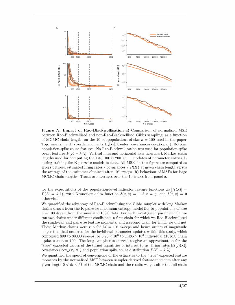
Figure A. Impact of Rao-Blackwellisation a) Comparison of normalised MSEbetween Rao-Blackwellised and non-Rao-Blackwellised Gibbs sampling, as a functionof MCMC chain length, on the 10 subpopulations of size n = 100 used in the paper.Top: means, i.e. first-order moments Eλ[xi], Center: covariances covλ(xi,xj), Bottom:population-spike count features. No Rao-Blackwellization was used for population-spikecount features P (K = k|λ). Vertical lines and horizontal axis ticks mark Markov chainlengths used for computing the 1st, 1001st 2001st, ... updates of parameter entries λlduring training the K-pairwise models to data. All MSEs in this figure are computed aserrors between estimated firing rates / covariances / P (K) at given chain length versusthe average of the estimates obtained after 106 sweeps. b) behaviour of MSEs for largeMCMC chain lengths. Traces are averages over the 10 traces from panel a.

for the expectations of the population-level indicator feature functions Eλ[fk(x)] =P (K = k|λ), with Kronecker delta function δ(x, y) = 1 if x = y, and δ(x, y) = 0otherwise.

We quantified the advantage of Rao-Blackwellising the Gibbs sampler with long Markovchains drawn from the K-pairwise maximum entropy model fits to populations of sizen = 100 drawn from the simulated RGC data. For each investigated parameter fit, weran two chains under different conditions: a first chain for which we Rao-Blackwellisedthe single-cell and pairwise feature moments, and a second chain for which we did not.These Markov chains were run for M = 106 sweeps and hence orders of magnitudelonger than had occurred for the invidivual parameter updates within this study, whichcomprised 800 to 30000 sweeps, or 3.96× 106 to 1.485× 106 individual MCMC chainupdates at n = 100. The long sample runs served to give an approximation for the”true” expected values of the target quantities of interest to us: firing rates Eλ[fi(x)],covariances covλ(xi,xj) and population spike count distribution P (K = k|λ).

We quantified the speed of convergence of the estimates to the ”true” expected featuremoments by the normalised MSE between sampler-derived feature moments after anygiven length 0 < m < M of the MCMC chain and the results we got after the full chain

4/27

length. After the full M = 106 sweeps, the Rao-Blackwellised and non-Rao-Blackwellisedestimates on average differed by 1.7× 10−4%, 0.013% and 4× 10−6% normalised MSEfor firing rates, covariances and population spike count distributions, respectively. Wecomputed the distance to ”truth” for each condition as the normalised MSE to theEλ[f(x)] averaged over both conditions. We obtained MCMC estimates for the featuremoments of the K-pairwise maximum entropy models fits to 10 subsampled populationsof n = 100 neurons each drawn from our retina simulation. Supplementary figure Aadisplays the results for the two conditions, Rao-Blackwellised vs. non-Rao-Blackwellised,for each of the 10 investigated fits.

MSEs of firing rate features Eλ[xi] did not benefit from Rao-Blackwellisation. Thisis expected, as each xi is sampled n − 1 times per sweep and thus the moments arealready well estimated relative to the second-order features. For covariances covλ(xi,xj),normalised MSEs showed clear improvement under Rao-Blackwellisation, visible as anapproximately constant offset between the avarages over all 10 parameter fits in theloglog-domain as seen in figure Ab. The normalised MSE on average was 3.19 timeshigher for non-Rao-Blackwellised (given by the downwards offset of the normalisedMSEs of the Rao-Blackwellised estimates). The fraction of samples needed from Rao-Blackwellised runs to achieve the same normalised MSE on the pariwise momentsthan non-Rao-Blackwellised runs (given by the leftward offset of the normalised MSEsof the Rao-Blackwellised) overall was 32.02%. The fraction ranged from 34.93% at800 sweeps to 31.74% at 30000 sweeps. The ratio of normalised MSEs was similarlystable, being 2.96 times higher at 800 sweeps and 3.27 times higher at 30000 sweeps fornon-Rao-Blackwellised samples than for Rao-Blackwellised ones.

1.2 Exploiting the structure of the K-pairwise feature functionsallows blockwise parameter updates.

As described in the previous section, we can use MCMC to obtain the expected valuesof the feature function Eλ[f(x)] that are needed to to optimise the model parameters

λ. To find the parameter setting λ which maximise the log-likelihood over the givendata vectors x(m), m = 1, . . . , M , we follow an iterative update scheme introducedpreviously [4], and extend it to the K-pairwise model. The update scheme optimisesparameter changes λnew−λold relative to a current parameter estimate λold, rather thanthe parameters λ directly. The benefit of this scheme over standard gradient ascent onthe regularised log-ligkelihood as in eq. (2) is that we can give closed-form solutions foroptimal values of a single component λl when temporarily holding all other componentsλ∼l fixed.

Changing the current parameter estimate λold to λnew leads to a change in log-likelihoodof

∆L(λnew, λold) =1

M

M∑m=1

logP (x(m)|λnew)− 1

M

M∑m=1

logP (x(m)|λold)

= (λnew − λold)>(

1

M

M∑m=1

f(x(m))

)− Eλold

[exp

((λnew − λold)>f(x)

)].

(4)

The only relevant expectations are w.r.t. the data distribution and P (x|λold), i.e. thecurrent parameter estimate. The term Eλold [exp

((λnew − λold)>f(x)

)] can be simplified

when restricting the update vector λnew−λold to be non-zero only in selected components.In the simplest case, only a single component λl is updated. In this case, the fact thatall components of the K-pairwise feature function f(x) are binary, allows to move the

5/27

exponent out of the expected value, a trick used by [4]:

The resulting single-coordinate updates only require the feature moments Eλold [fl(x)]:

Eλold [exp((λnew − λold)>f(x)

)] = Eλold [exp((λnewl − λoldl )fl(x)]

= Eλold [1 + (exp(λnewl − λoldl )− 1)fl(x)]

= 1 + (exp(λnewl − λoldl )− 1)Eλold [fl(x)].

Equation (4) can now be solved analytically for the single free component λnewl thatmaximises the change in log-likelihood. A closed-form optimal solution is still possiblewhen adding an l1-penalty to the log-likelihood [4]. We use this l1-regularised variant tocalculate the possible gain in penalized log-likelihood for each possible update of thesingle-cell (hi) and pairwise (Jij) feature moments E[xi] and E[xixj ], and then performthe update which yield the largest gain.

If we instead allow more than a single component l of the update λnewl − λoldl to benon-zero, we in general would have to deal with the term

Eλold

[∏l∈J

[1 + (exp(λnewl − λoldl )− 1)fl(x)]

],

which requires the higher-order moments Eλold[∏

l∈I fl(x)]

for all I ⊆ J and J ⊆{1, . . . , n} being the index set of components that are not set to zero.

The population spike-count features fk(x), however, are mutually exclusive (only one ofthe n+1 features can be non-zero at any time), and therefore we can update all parametersof V jointly, and still pull the exponenetial term outside of the expectation. For thepopulation-spike count features fk(x), hereafter collectively called fV (x) ∈ {0, 1}n+1, allsuch terms of order ||I|| > 1 are zero due to the sparsity of fV (x). When restricting thecurrent parameter update of λ to only update components corresponding to V , we have

∆L(V new, V old) = (V new − V old)>(

1

M

m∑m=1

fV (x(m))

)− Eλold [exp((V new − V old)>fV (x))]

and

Eλold [exp((V new − V old)>fK(x)

)] =

∑x

exp((V new − V old)>fK(x)

)P (x|λold)

=

n∑k=0

∑x:

∑i xi=k

exp((V newk − V oldk fKk (x)

)P (x|λold)

=n∑k=0

exp((V newk − V oldk )fKk (x)

) ∑x:

∑i xi=k

P (x|λold)

=

n∑k=0

exp((V newk − V oldk )fKk (x)

)P (k|λold).

We obtained estimates of the values of P (k|λold) = Eλold [fk(x)] from the MCMC sampleusing the indicator functions fk(x), and optimising w.r.t. V newk , k ∈ {1,. . . ,n} usinggradient-based methods [9].

In summary, our update-scheme for maximising the log-likelihood proceeds as follows:For a given parameter vector λold, we first estimate the expectation of the featurefunctions fi(x), fij(x) and fk(x) using a running average over an MCMC sampling andRao-Blackwellization. We then calculate, for each possible single-neuron parameter hi

6/27

and each possibly pairwise term Jij the gain in penalised log-likelihood that we would getfrom updating it, using methods as described above and derived in [4]. We additionallycompute the gain in penalised log-likelihood that would result from optimising all nof the free V parameters jointly, using a convex optimization. Finally, we choose theupdate that brings the largest gain, and either update a single hi, a single Jij , orall V parameters. Subsequently, we again estimate the new feature functions usingMCMC sampling given the current estimate of λold ← λnew before we update again.We initialised the algorithm assuming independent neurons (i.e. setting each hi usingthe firing rate of each neuron, and leaving J and V zero). The algorithm then typicallyfirst updated all V parameters, before proceeding to jump between different J , h and Vupdates.

# sweeps2000 4000 6000

ESM desila

mron %

0

20

40

60

80

100

120

true FR [Hz]0 5

mod

el e

stim

ate

0

5

true covariances0 0.05

0

0.05

true count0 0.4

0

0.4

stimulus conditioncb nat fff

% n

orm

alis

ed M

SE

0

2

4

6

a b

c

Figure B. Quality of fits for K-pairwise maximum entropy model acrossmultiple populations and stimulus conditions a) Normalised MSEs for firingrates, covariances and P (K) during parameter learning. Error values collapses across 10subpopulations at n = 100, fit to simulated activity in response to natural images, onepoint for each displayed iteration and each subpopulation. Lines are moving averages(smoothing kernel width = 150 param. updates). b) Quality of fit after parameterlearning. Data vs. model estimates for firing rates, covariances and P (K), collapsedover all 10 subpoplations with size n = 100. c) Quality of fit for different stimulus types.Normalised MSEs after maximum entropy model fitting shown for 10 subpopulationsfor natural images (nat) and 5 subpopulations each for checkerboard (cb) and full-fieldflicker (fff). All subpopulations of size n = 100. Vertical bars give averages. Colours asin a), b).

1.3 Effect of temperature on K-pairwise model statistics

We compute specific heat curves from the K-pairwise model by introducing a temperatureT that scales the learned parameters by 1

T , i.e. λT = λ/T . Temperature T = 1 corre-sponds to the statistics of the empirical data. By changing T to other parameter valuesone can perturb the statistics of the system [10]: For models fit to our simulated data,increasing temperature leads to models with higher firing rates and weaker correlations(Fig. C), with PT (x) approaching the uniform distribution for very large T . If thetemperature is decreased towards zero, PT (x) has most of its probability mass overthe most probable spike patterns. In many probabilistic systems, lowering T leads toincreasing correlations, as the systems then ’jumps’ between several different patterns

7/27

and thus the activation probabilities of different elements are strongly dependent on eachother. However, for the simulated RGC activity, the qualitative behaviour is different,and the sparsity of data leads to a decrease of correlations: At a bin size of 20 ms [11], themost probable state is the silent state, followed by patterns in which exactly one neuronsspikes. In an example population of size n = 100, 53.8% of observed spike patternscontain at most one spike. When decreasing the temperature to T < 1, patterns with atmost one spike dominate the systems even more strongly: For the same population andtemperature T = 0.8, we find 95.6% of observed patterns to contain at most one spike.Thus, when the temperature is lowered, the shift in probability mass to single-spikepatterns decreases correlations.

pop. spike count

mod

el p

roba

bilit

y

temperature temperature0 20 40

1

0

0.01

1 1.5 21.5 20

10

20 10 0

-2

-4

10

10

-610

T=1

mod

el F

R (

Hz)

mod

el c

ovs

Figure C. Temperature and population statistics for K-pairwise modelsChanging the temperature parameter scales firing rates (left), covariances (centre)and population spike-counts (right) of samples x generated from temperature-perturbedK-pairwise model fits.

time (h)

spec

ific h

eat 1

0.5

0

temperature1/32 1/8 1/2 2 8 1 1.5 2

Figure D. Estimating specific heat via MCMC sampling MCMC estimates ofspecific heat from a K-pairwise maximum entropy model fit to example population withn = 100. For every investigated temperature 0.8 ≤ T ≤ 2, we run a Markov Chain tosample from the temperature-perturbed maximum entropy model. Estimates were takenfrom the average over first 4h computation time of sampling (dashed vertical line).

2 Supplementary Text: Specific heat in simple mod-els

We refer to a maxmimum entropy model as ’flat’ if it is fully specified by the populationspike count distribution P (

∑ni=1 xi = k), i.e. the model class studied in [12–14]. In

this model class, all neurons have the same firing rate µ and pairwise correlation ρ. Asneuron identities become interchangeable, all

(nk

)possible patterns x with

∑ni=1 = k are

8/27

assigned the same probability P (k) = P (x)(nk

). In flat models, all relevant population

properties can be computed from summing over n+ 1 different spike counts, and onenever has to (explicitly) sum over the entire 2n possible spike patterns.

2.1 Independent neurons

A special case of a flat model is an independent model in which all neurons have thesame firing rates and zero correlations. Assuming independent spiking for each of then neurons and a shared probability q ∈ [0, 1] to fire in a time bin, the distribution ofpopulation spike counts k =

∑ni=1 xi is given by a binomial distribution,

P (x|q) = qk(1− q)n−k

P (k|q) =

(n

k

)qk(1− q)n−k.

To compute specific heat capacities for the underlying neural population of size n, wecan rewrite the binomial distribution in maximum entropy form

P (x|V ) =1

Z(V )exp (Vk)

P (k|V ) =1

Z(V )

(n

k

)exp (Vk) .

Re-introducing parameters Vk, k = 0, . . . , n, we find

Vk = logP (k|q)− log

(n

k

)+ logZ(V )

= k log(q) + (n− k) log(1− q)),

and for the heat capacity, we get

Var[logP (x|V )] = Var[k log(q) + (n− k) log(1− q)]= (log(q)− log(1− q))2 Var[k].

The binomial variance is Var[k] = nq(1 − q). We plug this in and see that at unittemperature T = 1, the specific heat is given by

c(T = 1) =1

nVar[logP (x|V )] = q(1− q)(log(q)− log(1− q))2, (5)

which is independent of population size n.

When explicitly introducing temperatures other than T = 1, we add a factor 1T = β that

scales the parameters V and renormalise, yielding

P (k|V, T ) =1

Z(βV )

(n

k

)exp(βVk),

where Vk, k = 0, ..., n is defined w.r.t. q as above. This is the same functional formas was given for the binomial distribution at T = 1, with only parameters V beingreplaced by βV . We can also go back to the standard binomial parametrisation with

qβ = qβ

qβ+(1−q)β and obtain

P (k|V, T ) =

(n

k

)qkβ(1− qβ)(n−k).

9/27

Changing the temperature T = 1β retains the binomial form of the population model,

and we can generalise the expression for the specific heat (5) of the independent flatmodel for any temperature T to be

c(T ) = qβ(1− qβ)(log(qβ)− log(1− qβ))2, (6)

which again is independent of the population size n. The independent flat model is acase that does not show divergent specific heat, and for which the peak of the heat isnot necessarily at unit temperature. Later, we will derive why this makes the binomialmodel one of only two non-critical special cases.

The independent model also allows to identify the location of the peak specific heat,c(T ∗), for q 6= 0.5. We have

δc

δβ= βqβ (1− qβ) log2

(q

1− q

)(2 + β log(

q

1− q) (1− 2qβ)

),

which for a given q has a root at β such that

qβ + (1− q)β

qβ − (1− q)β=

1

2log

(qβ

(1− q)β

).

An interesting question to ask is on which side of the unit temperature T = β = 1 thepeak of the specific heat is found. In this case, we seek a q such that the peak specificheat is found at β = 1. Note that these specific values for q come in pairs q, 1− q. Inthe context of binned spiking activity, we will focus on the smaller value in each suchpair. For the peak to be at unit temperature β = 1, we require

q = (1− q) exp

(1

q − 12

)≈ 0.0832. (7)

Assuming 20 ms temporal binning of activity data, this corresponds to an average firingrate of 4.16 Hz – higher than any firing rate in our simulated RGC population. Thepeak specific heat for independent populations (irregardless of the population size) witha firing rate below this value are found for T ∗ > 1 (see Fig. 3f). Populations with higheraverage firing rate have the peak specific heat at a temperature T ∗ < 1.

For the more general case of independent neurons but with different firing rates, we have

c(β) =1

n

n∑i=1

q(i)β (1− q(i)

β )(log(q(i)β )− log(1− q(i)

β ))2,

for q(i) = exp(hi)1+exp(hi)

and q(i)β =

(q(i))β/((q(i))β

+(1− q(i))β

).

2.2 Aside: Asymptotic entropy in flat models

To calculate the variance of log-probabilities, we first need the mean log-probability, i.e.the (negative) entropy.

10/27

Entropy: Recalling that P (k) = P (x)(nk

), the entropy of the flat model for general

P (k) can be written as

Hn = −∑x

P (x) logP (x)

= −∑k

∑x:

∑i xi=k

P (x) logP (x)

= −∑k

P (k)

(logP (k)− log

(n

k

)).

Thus, the entropy of a flat model is

Hn = −∑k

P (k)

(logP (k)− log

(n

k

)).

Asymptotic entropy: We assume that P (k) has a limiting distribution f(r), wherer ∈ [0, 1] is the probability density of a proportion of r neurons spiking simultaneously.Therefore, for large n

Hn = −∑k

P (k)

(logP (k)− log

(n

k

))≈ −

∑k

1

nf

(k

n

)(logP (k)− log

(n

k

))

≈ −∫ 1

0

f(r)

(log

f(r)

n− log

(n

nr

))dr

= −∫ 1

0

f(r) log f(r)dr + log(n) + n

∫ 1

0

f(r)η(r)dr.

Here, we used Stirling’s approximation to obtain, for large n,

log

(n

nr

)≈ n (−r log r − (1− r) log(1− r)) =: nη(r). (8)

As the first term is constant in n, the second term only grows with log(n), and the thirdwith n, we get that the entropy of a flat model, for large n, is given by

Hn = nh, (9)

with

h :=

∫ 1

0

f(r)η(r)dr. (10)

2.3 Asymptotic specific heat in flat models at unit temperature

Next, we calculate the specific heat, first exactly and then for large n, and finally forweakly correlated models:

First, the specific heat is given by

c(T = 1) =1

nVar[logP (x)] =

1

n

∑x

P (x) (logP (x)− E[logP (x)])2

=1

n

∑k

P (k)

(logP (k)− log

(n

k

)− E[logP (x)]

)2

.

11/27

Using E[logP (x)] = −Hn, we get that

c(T = 1) =1

n

∑k

P (k)

(logP (k)− log

(n

k

)+Hn

)2

or

=1

n

∑k

P (k)

(logP (k)− log

(n

k

))− 1

nH2n.

For large n, we have that P (k) ≈ 1nf(kn

). We get that

c(T = 1) =1

n

∑k

P (k)

(logP (k)− log

(n

k

)+Hn

)2

≈ 1

n

∑k

1

nf

(k

n

)(log

(1

nf

(k

n

))− log

(n

k

)+Hn

)2

≈ 1

n

∫ 1

0

f (r)

(log f (r)− log n− log

(n

nr

)+Hn

)2

dr

≈ 1

n

∫ 1

0

f (r) (log f (r)− log n− nη(r) + nhn)2dr

=1

n

∫ 1

0

f (r)(

(log f (r)− log n)2

+ n2 (η(r)− hN )2

+ 2n (log f (r)− log n) (hn − η(r)))dr

=1

n

∫ 1

0

f (r)(log2 f (r) + log f (r) (2n (hn − η(r))− 2 log n)

)dr

+1

n

∫ 1

0

f (r)(log2 n− n2 (hn − η(r))

)dr.

For large n, this integral is dominated by the term in n2, and thus the specific heat isasymptotically given by

c(T = 1) = n

∫ 1

0

f(r) (η(r)− h)2dr. (11)

Therefore, in general, the specific heat grows linearly, and hence diverges (see Fig.G). The only exception to this are models for which η(r) − hn = 0 for almost all r.This happens if f(r) is a delta-distribution, f(r) = δ(r − µ), in which case hn = η(µ)and therefore the integral vanishes. This occurs whenever the pairwise correlations donot grow proportionally with n2, as then the variance of the population spike countcollapses in the limit. One such special case is the binomial distribution over k, asalready demonstrated above using a more direct approach. There is a second specialcase, namely if f(r) is a combination of two δ-peaks at µ and 1−µ (See [13] for details)–this special case corresponds to a flat Ising model.

2.4 In flat models, specific heat does not diverge for tempera-tures which are not equal to 1:

Above we showed that at unit temperature, the specific heat for flat models (almost)always diverges. Now, we show that this is NOT true for any other temperature. Thisexplains that, for any f(r), we will find that the unit temperature is ’special’.

12/27

First, we calculate the spike-count distribution at any inverse temperature β:

Pβ(x) =1

ZβP (x)β

Pβ(k) =1

Zβ

(n

k

)1−β

P (k)β .

For large n,

fβ(r) ≈ nPβ(rn)

=n

Zβ

(n

nr

)1−β

P (rn)β

≈ n

Zβexp (n(1− β)η(r))P β(rn).

For large populations, this expression is dominated by the exponential exp (n(1− β)η(r)).For β < 1, the exponential term is in turn dominated by the mode of η(r), which is atr = 1

2 . Thus, for β < 1, fβ(r) = δ(r − 12 ), a delta-peak at r = 1

2 .

Conversely, for β > 1, the argument of the exponential has its peaks at r = 0 and r = 1,and therefore fβ(r) = 1

2δ(r − 1) + 12δ(r − 0). In this case, we also have that the integral

in the specific heat vanishes, and that the specific heat does not diverge.

3 Specific heat divergence rate in flat models as func-tion of correlation strength

In the next two sections, we will derive analytic expressions to predict the specificheat divergence rate in flat models as a function of the correlation strength within thepopulation. Starting out from eq. (11), we will use two different approximations tof(r) that will each yield results that allow us to better understand the behaviour of thespecific heat at unit temperature c(T = 1) in flat models.

3.1 Asymptotic entropy and specific heat in weakly correlatedflat models:

Next, we examine entropy and specific heat in models with weak correlations. If themodel is weakly correlated and its mode is not at 0 or 1 we can assume it to beapproximately Gaussian with mean µ and variance σ2,

f(r) =1

Zexp

(− 1

2σ2(r − µ)

2

).

We first calculate the entropy: We expand η(r) to second order around µ,

η(r) = η(µ+ δ) = η(µ) + η′(µ)δ +δ2

2η′′(µ) + ...,where

η′(r) = log

(1− rr

)η′′(r) =

−1

r(1− r),

13/27

hence

η(µ+ δ) = η(µ) + δ log

(1− µµ

)− δ2

2µ(1− µ)+ ...

=: α+ δβ + δ2γ.

Thus, the asymptotic entropy-rate is given by

h =

∫f(r)η(r)dr

= α+ 0β + γσ2

= η(µ)− 1

2µ(1− µ)σ2.

We further investigate the variance, again neglecting all terms which are of higher orderthan 2, obtaining

(η(µ+ δ)− h)2

=((α− h) + βδ + γδ2

)2= (α− h)2 + δ2β2 + 2(α− h)βδ + 2(α− h)γδ2 + 2(α− h)γδ2 + . . .

= (α− h)2 + δ (2(α− h)β) + δ2(β2 + 2(α− h)γ

)+ . . .

Integrating this expression over f(r), and dropping all terms in σ which are of orderhigher than 2, we get∫

f(r)(η(r)− h)2 = (α− h)2 + σ2(β2 + 2(α− h)γ

)=

σ4

µ2(1− µ)2+ σ2

(log2

(1− µµ

)− σ2

µ2(1− µ)2

)≈ σ2 log2

(1− µµ

).

In summary, we arrive at

c(T = 1) = nσ2 log2

(1− µµ

), (12)

and for small µ

c(T = 1) = nσ2 log2(µ).

In other words, a population of a given size n at fixed firing rate µ that has a high specificheat is simply a population which is very correlated. Inspecting the equations above,we see that the final results do not critically depend on the Gaussian assumption—theonly requirement for the calculation to be accurate is that the distribution is reasonablypeaked around its mean.

3.2 Asymptotic specific heat in the beta-binomial populationmodel

For the beta-binomial model, we assume f(r) to be given by a beta distribution, i.e.

f(r) =1

B(α, β)rα−1(1− r)β−1.

14/27

Such f(r) arise for large populations when the population spike count k is described bya beta-binomial distribution, and the choice for the beta distribution as a model for f(r)was motivated by the successful application of beta-binomial models P (k|α, β) to oursimulated RGC activity (see Fig. E, F).

For beta-distributed r, we have

E[r] =α

α+ β,

Var[r] =αβ

(α+ β)2(α+ β + 1),

E[log r] = γ(α)− γ(α+ β),

where γ denotes the digamma function.

α

0.35

0.4

0.45

population size20 160 300

β

11

13

15

pop. spike count60

freq

uenc

y

10 -3

10 -2

10 -1

10 0

40200

Tkacik et al. 2015Tkacik et al. 2012Okun et al. 2012Ioffe et al. 2016,

'water'

a b

Figure E. Beta-binomial models fit to spike-count distributions from litera-ture and our retina simulation a) Spike-count distributions published in previousstudies (dotted) and corresponding beta-binomial fits. As respective population sizes forthe beta-binomial distribution, we used the reported n = 120 for Tkacik et al. (2015),n = 40 for Tkacik et al. (2012), n = 96 for Okun et al. (2012), and n = 128 for Ioffe andBerry (2016). b) Beta-binomial parameters α, β for population subsampled from ourRGC simulation with different sizes n. Means ± 1 standard deviation over 100 randomsubsamples per population size.

The entropy can be calculated using known results on the expectation of the log,

h = γ(α+ β + 1)− α

α+ βγ(α+ 1)− β

α+ βγ(β + 1).

For the specific heat at unit temperature according to equation (11), we however alsorequire the expected values

E[r2 log2 r],E[(1− r)2 log2(1− r)],E[r(1− r) log r log(1− r)], (13)

i.e.

E[rk(1− r)l logm r logn(1− r)] =

∫ 1

0

f(r){rk(1− r)l logm r logn(1− r)}dr (14)

under beta-binomial distribution f(r), where k, l,m, n ∈ {0, 1, 2}.

15/27

Figure F. (No) Influence of beta-binomial approximation on heat capacitySpecific heat capacities computed from population spike count distributions P (K). Spikecount distributions for population sizes n = 20, . . . , 300 were obtained from 50 uniformlydrawn subpopulations each. Simulated retinal activity was taken from of the retinasimulation with in total N = 316 RGCs that responded to natural image stimulation.Resulting specific heat traces computed from a) beta-binomial approximations to thespike count distributions and b) from raw P (K) (right) do not display strong qualitativedifferences.

We begin the derivation of these terms by observing that

u(m,n)(r, α+ k, β + l) = log(r)mr(α+k−1) log(1− r)n(1− r)(β+l−1),

δ

δαu(m,n)(r, α+ k, β + l) = log(r)m+1r(α+k−1) log(1− r)n(1− r)(β+l−1)

= u(m+1,n)(r, α+ k, β + l),

δ

δβu(m,n)(r, α+ k, β + l) = log(r)mr(α+k−1) log(1− r)n+1(1− r)(β+l−1)

= u(m,n+1)(r, α+ k, β + l),

for any k, l ∈ N. Note that the exponents k, l are readily absorbed into new effectivebeta distribution parameters α′ = α+ k, β′ = β + l.

The triplets (u(m,n), u(m+1,n),u(m,n+1)) for any m,n ∈ N recursively express the inte-grands of (14) as continuous derivatives, which allows us to repeatedly apply Leibniz’rule to the integral. We first deal with E[rk logm r], where m = k = 2, n = l = 0,α′ = α+ 2, β′ = β, which is the first of the three expected values we need to compute

16/27

the specific heat at unit temperature:

Beta(α, β)E[r2 log2 r] =

∫ 1

0

rα−1(1− r)β−1 log2(r)r2dr

=

∫ 1

0

δ2

δα2{rα+1(1− r)β−1}dr

=

∫ 1

0

δ

δα{ δδα{rα+1(1− r)β−1}}dr

=δ

δα

∫ 1

0

δ

δα{rα+1(1− r)β−1}dr

=δ2

δα2

∫ 1

0

rα+1(1− r)β−1dr

=δ2

δα2Beta(α+ 2, β).

The first two derivatives of Beta(α′, β′) w.r.t. α are given by

δ

δαBeta(α′, β′) = Beta(α′, β′)(ψ0(α′)− ψ0(α′ + β′)),

δ2

δα2Beta(α′, β′) = Beta(α′, β′)

((ψ0(α′)− ψ0(α′ + β′))2 + ψ1(α′)− ψ1(α′ + β′)

).

We obtain the m-th derivative also for m > 2 using an iterative rule. The beta-binomialnormaliser Beta(α′, β′) furthermore cancels out with the denominator Beta(α, β) of theoriginal beta distribution through

Beta(α+ k, β + l) =

∏k−1i=0 (α+ i)

∏l−1j=0(β + j)∏k+l−1

i=0 (α+ β + i)Beta(α, β).

Combining the previous results gives

E[r2 log2 r] =1

Beta(α, β)

∫ 1

0

rα−1(1− r)β−1log2(r)r2dr (15)

=1

Beta(α, β)

δ2

δα2Beta(α+ 2, β)

=α(α+ 1)

(α+ β)(α+ β + 1)

1

Beta(α+ 2, β)

δ2

δα2Beta(α+ 2, β)

=α(α+ 1)

((ψ0(α+ 2)− ψ0(α+ β + 2))2 + ψ1(α+ 2)− ψ1(α+ β + 2)

)(α+ β)(α+ β + 1)

.

For m = 2, k = 1, n, l = 0 the result

E[r log2 r] =α

α+ β[(ψ0(α+ 1)− ψ0(α+ β + 1))2 + ψ1(α+ 1)− ψ1(α+ β + 1)]

is identical to the one from [15] in the appendix A.3, eq. (28).

We have Beta(α, β) = Beta(β, α), i.e. the above equations hold symmetrically for αand β interchanged, and n, l instead of m, k. This gives us the second required term tocompute the specific heat at unit temperature,

E[(1− r)2 log2(1− r)] (16)

=β(β + 1)

((ψ0(β + 2)− ψ0(α+ β + 2))2 + ψ1(β + 2)− ψ1(α+ β + 2)

)(α+ β)(α+ β + 1)

.

17/27

Including derivatives w.r.t. both α and β, we more generally arrive at

E[log(r)mrk log(1− r)n(1− r)l] =

∏k−1i=0 (α+ i)

∏l−1j=0(β + j)∏k+l−1

i=0 (α+ β + i)g(m,n)(α+ k, β + l).

We get recursive formulas for g(m,n), starting at g(0,0)(α, β) = 1:

g(m+1,n)(α, β) = (ψ0(α)− ψ0(α+ β)) g(m,n)(α, β) +δ

δαg(m,n)(α+ β)

g(m,n+1)(α, β) = (ψ0(β)− ψ0(α+ β)) g(m,n)(α, β) +δ

δβg(m,n)(α+ β).

To compute c(T = 1), we still require the case of m = k = n = l = 1 given by

E[r(1− r) log(r) log(1− r)] =αβ

(α+ β)(α+ β + 1)g(1,1)(α+ 1, β + 1), (17)

with

g(1,1)(α+ k, β + l) = ψ0(α+ k)ψ0(β + l)− ψ0(α+ β + k + l) (ψ0(α+ k) + ψ0(β + l))

+ ψ0(α+ β + k + l)2 − ψ1(α+ β + k + l). (18)

Combining the results of equations (15), (16), (17), (18) with eq. (11), we arrive at

c(T = 1)

n=

∫ 1

0

f(r) (η(r)− h)2dr

=α(α+ 1)ψ1(α+ 1) + β(β + 1)ψ1(β + 1)

(α+ β)(α+ β + 1)

+αβ (ψ0(α+ 1)− ψ0(β + 1))

2

(α+ β)2(α+ β + 1)− ψ1(α+ β + 1)

= Var[r] (ψ0(α+ 1)− ψ0(β + 1))2 − ψ1(α+ β + 1).

3.3 Effects of firing rates

In our flat model analyses, we considered neural populations with various sizes andaverage correlation strengths and usually treated firing rates as fixed, generally at therate of 1.5 Hz [16]. In general, however, different experimental stimuli may inducedifferent average firing rates within the populations. Our analytic predictions from 3.1and 3.2 for the divergence rate of specific heat can be evaluated for various combinationsof average correlation and average firing rate (Fig. H). Our predictions show that forthe systems with firing rates around 1.5 Hz, the specific heat divergence rates indeeddepends on average firing rates for a wide range of correlations strengths, albeit weakly.Thus comparisons of exact specific heat values across different experimental conditionsalso need to take differences in firing rates into account.

3.4 Specific heat divergence at clamped firing rates

Changes in temperature T scale all model parameters of the maximum entropy model,and thus in general affect firing rates, correlations and population spike count statistics.

For flat models, varying T during the specific heat analysis explores the behaviourthrough one-dimensional family of models parametrised by 1

T V ∈ Rn+1. Moving along

18/27

prob

abili

ty

temperature

spec

ific

heat

0.7 1 1.2

pop. spike count

0.2

0.1

00 100 200 300

ytilibaborp

5

10 30028026024022020018016014012010080604020

Figure G. Diverging specific heat for a non-natural spike-count distributionThe values of the population spike count distribution P (K) obtained from the retinalsimulation with N = 316 in response to natural image stimulation (orange, inset) wereshuffled (black trace, inset) across K, to yield a ’pathological’ P (K). We simulated datafor this P (K) from a flat model, and subsampled subpopulations of size n = 20, . . . , 300.The specific heat traces computed from this data also diverges and has a peak at unittemperature

this trajectory, we can explore a range of possible average correlation strengths ρ betweenthe entries of spike patterns x ∈ Rn: from the average correlation strength found in thedata at T = 1, to usually larger ρ for T → 0, and to ρ→ 0 for T →∞. However, notonly the correlations ρ change with T , but the firing rate 1

nE[K] is also affected.

We showed that the specific heat diverges whenever T = 1, and that it does not divergeotherwise. Is this also true if one ’clamps’ firing rates such that they are not altered bychanging T?

Tkacik et al. [16] introduced a modified temperature analysis for the K-pairwise maximumentropy model: After changing T , they numerically optimized the h parameters (hi(T ))such that the firing rates were not affected by temperature:

logPT (x|λ) =∑i

hi(T )xi +1

T

∑ij

Jijxixj + Vk

− logZ(J, V, h(T )), (19)

for k =∑ni=1 xi. The adjusted firing rate parameters hi(T ) are recomputed for each

temperature T and for each neuron i to keep the resulting firing rates E λT

[xi] fixed to

those firing rates obtained at T = 1.

We here show that for flat models, this result will be generically true: Specific heatdiverges whenever T = 1, even for a modified analysis in which firing rates are clamped:The flat model assumes all hi = h, Jij = J to be identical. Hence we can achieve suchan altered temperature scaling for the flat model by introducing a linear term h(T )k to

19/27

1 2 3 4 5c(

T=1)

/ n

10 -5

10 -4ρ= 0.0001

appr.exact

1 2 3 4 5

10 -4

10 -3ρ= 0.001

1 2 3 4 5

c(T=

1) /

n

10 -3

10 -2ρ= 0.01

1 2 3 4 510 -3

10 -2

10 -1ρ= 0.1

firing rate [Hz] firing rate [Hz]

Figure H. Specific heat divergence and average firing rate in flat modelsSpecific heat divergence rates c = c(T = 1)/n in flat models for fixed average correlationstrengths ρ and under various firing rates. Traces computed for general flat models usingthe approximate asymptotic prediction (12) (red, valid for small correlation strengthsρ), and for beta-binomial models using the asymptotically exact formula (19) (orange).Dashed vertical line marks 1.5 Hz, corresponding to the average firing rate of our retinasimulation under stimulation with natural images.

the model log-likelihood,

logPT (k|V ) =VkT− h(T )k + log

(n

k

)− logZ(V, h(T )). (20)

The scalar factor h(T ) for temperature T is chosen such that that the average firing rate1nET [K] is identical to that of the data (at T = 1), i.e. ET [K] = E1[K].

We repeated the specific heat analysis on our simulated RGC data with this adjustment.We found the same qualitative features in the specific heat traces obtained for differentpopulation sizes n: The peak of the curves diverges as the population size n is increased,and moves closer to unit temperature for increasing n (Fig. I). We also see that betweenthe different experimental stimuli, there is an increase in the slope of the specific heatdivergence from checkerboard stimuli (short-range spatial correlations, weak averagecorrelations, Fig. Ia) to full-field flicker (infinite-range correlations, strong averagecorrelations, Fig. Ic).

The derivations on specific heat divergence in section 2 also apply for the analysis withclamped firing rates: In particular, the specific heat will still diverge at unit temperatureunder the same conditions as before, since the original and the firing rate-preservingtemperature scalings coincide at T = 1, i.e. h(T = 1) = 0. For any other temperatureT = 1

β 6= 1, for fixed β, V , we can rewrite equation 20 as

Pβ(k) =1

Zβ

(n

k

)exp(Vk)β exp

(−hk

)=

1

Zβ

(n

k

)1−β

exp(−hk)1−βP (k)β ,

where we dropped explicit dependencies of PT (k|V ) on V and of h on β, as well as those

20/27

inverse temperature

1 1.5 2

specific

heat

0

2

4

a) checkerboard stimulus

n

20 100 200 300

c

1

3

5

max c

c at T=1

inverse temperature

1 1.5 2

specific

heat

0

2

4

6

b) natural stimulus

n

20 100 200 300

c1

3

5

7

max c

c at T=1

inverse temperature

1 1.5 2

specific

heat

0

5

10

c) full-field flicker

n

20 100 200 300

c

2

6

10 max c

c at T=1

Figure I. Signatures of criticality in flat models with clamped firing ratesSpecific heat capacities computed from beta-binomial approximations to populationspike-count distributions P (K) with clamped firing rates. For each temperature T , weadjusted the model to keep the average firing rate fixed to the average firing rate ofT = 1. Spike-count distributions for population sizes n = 20, . . . , 300 for each n wereobtained from 50 subpopulations drawn uniformly from our RGC simulation. Specificheat values are averages over subpopulations. Panels show averaged specific heat tracesas a function of 1

T for each population n (left), and average specific heat values at peakand at T = 1 (right), for a) checkerboard stimuli, b) natural stimuli and c) full-fieldflicker stimuli.

of Z for notational clarity. In the large-n approximation k = rn, the above becomes

fβ(r) ≈ n

Zβexp

(n(1− β){η(r)− hr}

)P (rn)β .

21/27

The latter equation for large n again is dominated by the exponential term

exp(n(1− β){η(r)− hr}

)= exp (n(1− β)η(r)) .

The inner function in r, η(r) = η(r)− hr, has its mode at r = 11+exp(h)

∈]0, 1[.

Plugging r into η(r) shows that the value attained at the mode is

η(r) = −h+ log(1 + exp h

),

which is zero if and only if h = log(1 + exp h

), i.e. if and only exp h = 1+exp h or 1 = 0.

Hence, η(r) 6= 0 for all h ∈ R and all β 6= 1. Thus, for large n, either fβ(r) ≈ δ(r − r),or fβ(r) ≈ 1

2δ(r − 1) + 12δ(r − 0), and the integral in the specific heat vanishes in either

case.

4 Correlations under uniform subsampling

In previous sections, we derived the dependence of the specific heat divergence oncorrelation strength in populations.

For the methods developed in [16], uniformly random subsampling of n many neuronsfrom a large fixed recording of size N was used to obtain several subpopulation at eachpopulation size. In terms of average correlations, we can formulate this subsamplingprocess as selecting n × n principal submatrices from a large fixed N × N matrixdescribing the correlations of N many random variables. The average correlation of thesubpopulation is the average over the respective selected entries. We denote the full indexset for N many random variables as [N ] = {1, . . . , N}. Let In = {I ⊆ [N ] : |I| = n}be the set of all size-n subpopulations of the full size-N recording. Let ρij be thecorrelation between variables indexed with i, j ∈ [N ]. We define the average correlationof a subpopulation I ∈ In as

ρn(I) :=2

n(n− 1)

∑i,j∈I,i<j

ρij =1

n(n− 1)

∑i,j∈I,i6=j

ρij .

We exclude diagonal entries ρii = 1 ∀i ∈ I.

In the following sections, we derive some basic results on the behaviour of averagecorrelation ρn(I) for uniformly sampled subsets I of N many random variables. We areprimarily interested in the mean E[ρn] and variance Var[ρn] of the average correlation

with respect to the uniform distribution over subsets Pn(I) =(Nn

)−1. We will see that

the mean E[ρn] is equal to the average correlation of the full recording ρn([N ]) for allsubpopulation sizes n– this is not surprising, as the entries of the sub-matrix are randomlysampled from ρij, and characterize how the Var[ρn] decreases to zero with increasingn. Taken together, this predicts that in terms of average correlation, uniformly drawnsubpopulations will quickly all behave like the full recording with increasing populationsize n, and the conditions for linear divergence of the specific heat derived in 2 arewell-met even for sizes n that are actually experimentally accessible.

4.1 Scaling of average correlation with population size underuniform subsampling

Expected mean correlation: Under uniform subsampling, the expected mean corre-lation strength E[ρn] of populations of any size n ≤ N is equal to the average correlationρN ([N ]) of the entire recording [N ], regardless of the exact correlation structure structure

22/27

{ρij}ij , i 6= j. This is simply a consequence of the fact that the entries of the submatrixare randomly (but not independently) drawn from the big correlation matrix. Moreformally:

Proof: The expected mean correlation across populations of fixed size n for uniformly

drawn populations(∀I ∈ In : Pn(I) =

(Nn

)−1)

is given by

E[ρn] =∑I∈In

Pn(I)ρn(I)

=

(N

n

)−1 ∑I∈In

ρn(I)

=

(N

n

)−12

n(n− 1)

∑I∈In

∑i,j∈I,i<j

ρij

=

(N

n

)−12

n(n− 1)

∑i,j∈[N ],i<j

(N − 2

n− 2

)ρij (21)

=2

N(N − 1)

∑i,j∈[N ],i<j

ρij

= ρN ([N ]). (22)

For line 21, we used that there are exactly(N−2n−2

)many subsets I ⊆ [N ] of size n that

contain a fixed pair of distinct variables i, j ∈ [N ], i 6= j.

Variance of mean correlation: Characterising the variance is a bit more involved,as subsampling a principal matrix is not the same as drawing entries independently,so it is not a-priori clear that the variance will drop as 1/n. However, under uniformsubsampling, the variance of mean correlation Var[ρn] decreases with population size nat least as Var[ρn] ∝ 1

n .

Proof: We begin with the second moment,

E[ρ2n] =

∑I∈In

Pn(I)ρ2n(I)

=

(N

n

)−1 ∑I∈In

ρ2n(I)

=

(N

n

)−1 ∑I∈In

2

n(n− 1)

∑i,j∈I,i<j

ρij

2

=

(N

n

)−14

n2(n− 1)2

∑I∈In

∑i,j,k,l∈I:i<j,k<l

ρijρkl. (23)

The four-index inner sum in 23 is problematic because the number of unique indices|{i} ∪ {j} ∪ {k} ∪ {l}| =: q for any valid quartet i, j, k, l can range between two (ifi = k, j = l) and four. We split the set of index quartets i, j, k, l depending on how manyof the indices are unique. Let

S2q (I) =

∑i,j,k,l∈I,i<j,k<l,|{i}∪{j}∪{k}∪{l}|=q

ρijρkl.

23/27

Conveniently, ∑i,j,k,l∈I,i<j,k<l

ρijρkl = S22(I) + S2

3(I) + S24(I)

and∑I∈In

∑i,j,k,l∈I:i<j,k<l

ρijρkl =∑I∈In

S24(I) +

∑I∈In

S23(I) +

∑I∈In

S22(I)

=

(N − 4

n− 4

)S2

4([N ]) +

(N − 3

n− 3

)S2

3([N ]) +

(N − 2

n− 2

)S2

2([N ]).

(24)

For the last equality, we again used that there are(N−qn−q

)possible size-n subsets of [N ]

that contain a specific set of q many unique indices.

Assuming n ≥ 4, plugging 24 into 23 yields

E[ρ2n] =

4

n(n− 1)N(N − 1)

((n− 2)(n− 3)

(N − 2)(N − 3)S2

4([N ]) +(n− 2)

(N − 2)S2

3([N ]) + S22([N ])

).

Rewriting the squared first moment as

E[ρn]2 =4

N2(N − 1)2

(S2

4([N ]) + S23([N ]) + S2

2([N ]))

(25)

allows to obtain

Var[ρn] = E[ρ2n]− E[ρn]2

= m24([N ])γ4,N (n) +m2

3([N ])γ3,N (n) +m22([N ])γ2,N (n), (26)

with

m24([N ]) =

4

N(N − 1)(N − 2)(N − 3)S2

4([N ]),

m23([N ]) =

1

N(N − 1)(N − 2)S2

3([N ]),

m22([N ]) =

2

N(N − 1)S2

2([N ]),

γ4,N (n) =(n− 2)(n− 3)

n(n− 1)− (N − 2)(N − 3)

N(N − 1),

γ3,N (n) =4(n− 2)

n(n− 1)− 4(N − 3)

N(N − 1),

γ2,N (n) =2

n(n− 1)− 2

N(N − 1).

The space of variance traces Var[ρn] ∈ RN lies within the span of the vectors γq,N (n), q ∈{2, 3, 4}. It is γ2,N + γ3,N + γ4,N ≡ 0 for all N > 1. The respective coordinates for agiven N ×N correlation matrix are given by the normalised summary statistics m2

q([N ])of that particular correlation matrix (see Fig. J).

For a coarse bound on the scaling of variance of the mean correlation, we once more

24/27

rewrite

Var[ρn] = d+e

n− 1+

f

n(n− 1), (27)

d =4

N − 3

(E[ρij ]

2 −m23([N ])

)− 2Var[ρij ]

(N − 2)(N − 3),

e =4(N + 1)

N − 3

(m2

3([N ])− E[ρij ]2)

+8Var[ρij ]

(N − 2)(N − 3),

f =8N

N − 3

(E[ρij ]

2 −m23([N ])

)+

2N(N − 5)Var[ρij ]

(N − 2)(N − 3),

where we expressed m24([N ]) through E[ρij ],Var[ρij ] and m2

3([N ]) via eq. 25. The exactscaling behaviour of Var[ρn] for n << N thus depends on the values for d, e, f , which forany given correlation structure {ρij} are fixed constants independent of n. The variancein any case decreases with n at least as fast as 1

n−1 . For

m23([N ]) ≈ E[ρij ]

2 − 2Var[ρij ]

(N + 1)(N − 2), (28)

we have e ≈ 0 and obtain Var[ρn] ∝ N(N−1)n(n−1) − 1, which initially decays as just as

independent sampling of correlation matrix entries (i.e. ∝ 1n(n−1) ) before eventually

decreasing to exactly zero for n = N . Decay accelerates as n approaches N because theuniform subsampling scheme draws variables without replacement. See figure J for anexample with N = 100 and an exponentially decaying spatial correlation profile thatleads to d = −7.25e-7, e = −5.84e-5, f = 0.013, i.e. e << f .

20 40 60 80 100

20

40

60

80

100 0

0.05

0.1

0.15

0.2

0.25

n0 20 40 60 80 100

var[ρ n]

10 -8

10 -6

10 -4

10 -2predictionsamples~ 1/(n-1)~ 1/(n(n-1))

a) b)

Figure J. Variance of mean for uniformly subsampled population of size n a)

Example correlation matrix for N = 100 neurons, ρij = 10.2527 exp

(− |i−j|

2

0.125

)(diagonal

removed for displaying purposes). b) Variance of average correlation Var[ρn]. Predictionsfrom 4.1 with statistics E[ρij ],Var[ρij ],m

23([N ]) computed from the matrix in a. Black

circles give variance over empirical average correlations for 10000 populations uniformlydrawn for each n = 2, 10, 20, 30, . . . , 90.

4.2 Specific heat and non-random subsampling for the full K-pairwise model

We asked whether our analytical results on effects of the subsampling scheme for flatmodels also hold empirically for the more powerful K-pairwise models. To this end, we

25/27

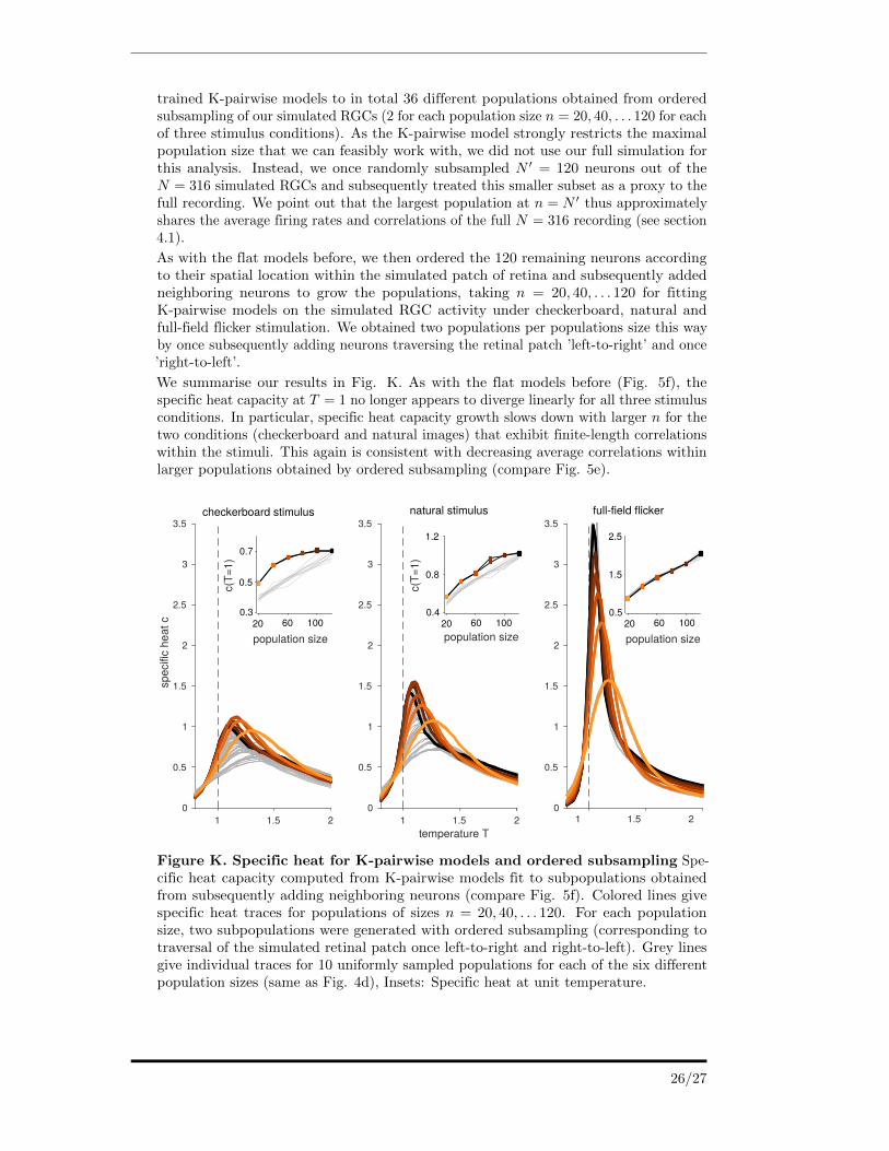
trained K-pairwise models to in total 36 different populations obtained from orderedsubsampling of our simulated RGCs (2 for each population size n = 20, 40, . . . 120 for eachof three stimulus conditions). As the K-pairwise model strongly restricts the maximalpopulation size that we can feasibly work with, we did not use our full simulation forthis analysis. Instead, we once randomly subsampled N ′ = 120 neurons out of theN = 316 simulated RGCs and subsequently treated this smaller subset as a proxy to thefull recording. We point out that the largest population at n = N ′ thus approximatelyshares the average firing rates and correlations of the full N = 316 recording (see section4.1).

As with the flat models before, we then ordered the 120 remaining neurons accordingto their spatial location within the simulated patch of retina and subsequently addedneighboring neurons to grow the populations, taking n = 20, 40, . . . 120 for fittingK-pairwise models on the simulated RGC activity under checkerboard, natural andfull-field flicker stimulation. We obtained two populations per populations size this wayby once subsequently adding neurons traversing the retinal patch ’left-to-right’ and once’right-to-left’.

We summarise our results in Fig. K. As with the flat models before (Fig. 5f), thespecific heat capacity at T = 1 no longer appears to diverge linearly for all three stimulusconditions. In particular, specific heat capacity growth slows down with larger n for thetwo conditions (checkerboard and natural images) that exhibit finite-length correlationswithin the stimuli. This again is consistent with decreasing average correlations withinlarger populations obtained by ordered subsampling (compare Fig. 5e).

temperature T1 1.5 2

spec

ific

heat

c

0

0.5

1

1.5

2

2.5

3

3.5checkerboard stimulus

1 1.5 20

0.5

1

1.5

2

2.5

3

3.5natural stimulus

1 1.5 2

population size20 60 100

c(T=

1)

20 60 10020 60 100

1.2

0.8

0.4

0.7

0.5

0.3

c(T=

1)

0.5

1.5

2.5

population sizepopulation size

0

0.5

1

1.5

2

2.5

3

3.5full-field flicker

Figure K. Specific heat for K-pairwise models and ordered subsampling Spe-cific heat capacity computed from K-pairwise models fit to subpopulations obtainedfrom subsequently adding neighboring neurons (compare Fig. 5f). Colored lines givespecific heat traces for populations of sizes n = 20, 40, . . . 120. For each populationsize, two subpopulations were generated with ordered subsampling (corresponding totraversal of the simulated retinal patch once left-to-right and right-to-left). Grey linesgive individual traces for 10 uniformly sampled populations for each of the six differentpopulation sizes (same as Fig. 4d), Insets: Specific heat at unit temperature.

26/27

References

1. Broderick T, Dudik M, Tkacik G, Schapire RE, Bialek W. Faster solutions of theinverse pairwise Ising problem. arXiv. 2007;0712.2437v2.

2. Rasmussen C, Williams C. Gaussian Processes for Machine Learning. MIT Press;2006.

3. Broderick T. Construction of a pairwise Ising distribution over a large state spacewith sparse data. Princeton University; 2007.

4. Dudik M, Phillips SJ, Schapire RE. Performance guarantees for regularizedmaximum entropy density estimation. In: Learning Theory. Springer; 2004. p.472–486.

5. Radhakrishna Rao C. Information and accuracy attainable in the estimation of sta-tistical parameters. Bulletin of the Calcutta Mathematical Society. 1945;37(3):81–91.

6. Blackwell D. Conditional expectation and unbiased sequential estimation. TheAnnals of Mathematical Statistics. 1947;p. 105–110.

7. Berkson J. Tests of significance considered as evidence. Journal of the AmericanStatistical Association. 1942;37(219):325–335.

8. Carlson D, Stinson P, Pakman A, Paninski L. Partition Functions from Rao-Blackwellized Tempered Sampling. arXiv preprint arXiv:160301912. 2016;.

9. Schmidt M. minFunc: unconstrained differentiable multivariate optimization inMatlab; 2005. http://www.cs.ubc.ca/~schmidtm/Software/minFunc.html.

10. Kirkpatrick S, Gelatt CD, Vecchi MP, et al. Optimization by simulated annealing.science. 1983;220(4598):671–680.

11. Schneidman E, Berry MJn, Segev R, Bialek W. Weak pairwise correlationsimply strongly correlated network states in a neural population. Nature.2006;440(7087):1007–12.

12. Amari Si, Nakahara H, Wu S, Sakai Y. Synchronous firing and higher-orderinteractions in neuron pool. Neural Computation. 2003;15(1):127–142.

13. Macke JH, Opper M, Bethge M. Common input explains higher-order correlationsand entropy in a simple model of neural population activity. Physical ReviewLetters. 2011;106(20):208102.

14. Tkacik G, Marre O, Mora T, Amodei D, Berry II MJ, Bialek W. The simplestmaximum entropy model for collective behavior in a neural network. Journal ofStatistical Mechanics: Theory and Experiment. 2013;2013(03):P03011.

15. Archer E, Park IM, Pillow JW. Bayesian entropy estimation for countable discretedistributions. The Journal of Machine Learning Research. 2014;15(1):2833–2868.

16. Tkacik G, Mora T, Marre O, Amodei D, Palmer SE, Berry MJ, et al. Thermody-namics and signatures of criticality in a network of neurons. Proceedings of theNational Academy of Sciences. 2015;112(37):11508–11513.

27/27